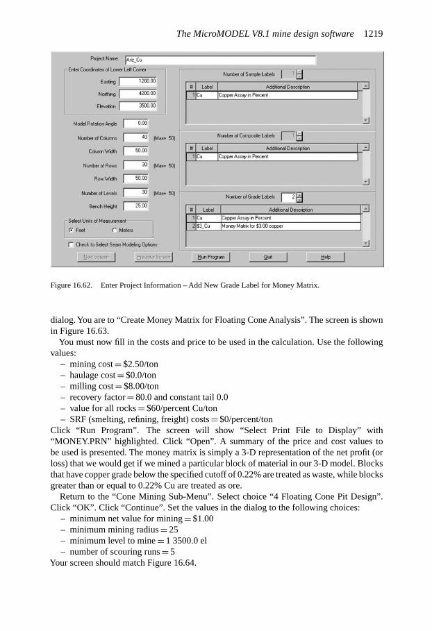
Embed Size (px)
Citation preview

Building on the success of its 2006 predecessor, this 3rd edition of OpenPit Mine Planning and Design has been both updated and extended,ensuring that it remains the most complete and authoritative account of mo-dern open pit mining available. Five new chapters on unit operations havebeen added, the revenues and costs chapter has been substantially revisedand updated, and the references have been brought fully up to date. In addi-tion, the pack now also includes a fully working version of the MicroMODELmine planning software package.
Volume 1 deals with the fundamental concepts involved in the planningand design of open pit mines. Subjects covered are mine planning, miningrevenues and costs, orebody description, geometrical considerations, pit limits,production planning, mineral resources and ore reserves, responsible mining,rock blasting, rotary drilling, shovel loading, haulage trucks and machine availability and utilization.
Volume 2 includes CSMine and MicroMODEL, user-friendly mine planningand design software packages developed specifically to illustrate the prac-tical application of the involved principles. It also comprises the CSMineand MicroMODEL tutorials and user’s manuals and eight orebody caseexamples, including drillhole data sets for performing a complete open pitmine evaluation.
Open Pit Mine Planning and Design is an excellent textbook for coursesin surface mine design, open pit design, geological and excavation enginee-ring, and in advanced open pit mine planning and design. The principlesdescribed apply worldwide. In addition, the work can be used as a practicalreference by professionals. The step-by-step approach to mine design andplanning offers a fast-path approach to the material for both undergraduateand graduate students. The outstanding software guides the student throughthe planning and design steps, and the eight drillhole data sets allow thestudent to practice the described principles on different mining properties(three copper properties, three iron properties and two gold properties).The well-written text, the large number of illustrative examples and casestudies, the included software, the review questions and exercises and thereference lists included at the end of each chapter provide the student withall the material needed to effectively learn the theory and application of openpit mine planning and design.
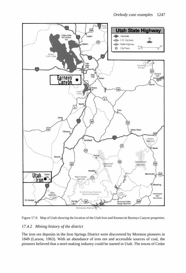
Photograph: BINGHAM CANYON mine. Courtesy of Kennecott Utah Copper.
W. HUSTRULID, M. KUCHTA AND R. MARTIN
OPEN PIT MINEPLANNING & DESIGN
an informa business
OPENPITMINEPLA
NNING&DESIGN
1
3R
DE
DITIO
NHUSTR
ULID
KUCHTA
MARTIN
1. FUNDAMENTALS3RD EDITION
Hustrulid_Vol1.qxd:Opmaak 1 22-05-13 11:41 Pagina 1

OPEN PIT MINE PLANNING & DESIGNVOLUME 1 – FUNDAMENTALS

This page intentionally left blankThis page intentionally left blank

OPEN PIT MINEPLANNING & DESIGNVolume 1 – Fundamentals
WILLIAM HUSTRULIDProfessor Emeritus, Department of Mining Engineering, University of Utah,Salt Lake City, Utah, USA
MARK KUCHTAAssociate Professor, Department of Mining Engineering, Colorado School of Mines,Golden, Colorado, USA
R. MARTINPresident, R.K. Martin and Associates, Inc., Denver, Colorado, USA

CRC PressTaylor & Francis Group6000 Broken Sound Parkway NW, Suite 300Boca Raton, FL 33487-2742
© 2013 by Taylor & Francis Group, LLCCRC Press is an imprint of Taylor & Francis Group, an Informa business
No claim to original U.S. Government worksVersion Date: 20130709
International Standard Book Number-13: 978-1-4822-2117-6 (eBook - PDF)
This book contains information obtained from authentic and highly regarded sources. Reasonable efforts have been made to publish reliable data and information, but the author and publisher cannot assume responsibility for the valid-ity of all materials or the consequences of their use. The authors and publishers have attempted to trace the copyright holders of all material reproduced in this publication and apologize to copyright holders if permission to publish in this form has not been obtained. If any copyright material has not been acknowledged please write and let us know so we may rectify in any future reprint.
Except as permitted under U.S. Copyright Law, no part of this book may be reprinted, reproduced, transmitted, or uti-lized in any form by any electronic, mechanical, or other means, now known or hereafter invented, including photocopy-ing, microfilming, and recording, or in any information storage or retrieval system, without written permission from the publishers.
For permission to photocopy or use material electronically from this work, please access www.copyright.com (http://www.copyright.com/) or contact the Copyright Clearance Center, Inc. (CCC), 222 Rosewood Drive, Danvers, MA 01923, 978-750-8400. CCC is a not-for-profit organization that provides licenses and registration for a variety of users. For organizations that have been granted a photocopy license by the CCC, a separate system of payment has been arranged.
Trademark Notice: Product or corporate names may be trademarks or registered trademarks, and are used only for identification and explanation without intent to infringe.
Visit the Taylor & Francis Web site athttp://www.taylorandfrancis.com
and the CRC Press Web site athttp://www.crcpress.com

Contents
PREFACE xv
ABOUT THE AUTHORS xix
1 MINE PLANNING 1
1.1 Introduction 11.1.1 The meaning of ore 11.1.2 Some important definitions 2
1.2 Mine development phases 51.3 An initial data collection checklist 71.4 The planning phase 11
1.4.1 Introduction 111.4.2 The content of an intermediate valuation report 121.4.3 The content of the feasibility report 12
1.5 Planning costs 171.6 Accuracy of estimates 17
1.6.1 Tonnage and grade 171.6.2 Performance 171.6.3 Costs 181.6.4 Price and revenue 18
1.7 Feasibility study preparation 191.8 Critical path representation 241.9 Mine reclamation 24
1.9.1 Introduction 241.9.2 Multiple-use management 251.9.3 Reclamation plan purpose 281.9.4 Reclamation plan content 281.9.5 Reclamation standards 291.9.6 Surface and ground water management 311.9.7 Mine waste management 321.9.8 Tailings and slime ponds 331.9.9 Cyanide heap and vat leach systems 331.9.10 Landform reclamation 34
V

VI Open pit mine planning and design: Fundamentals
1.10 Environmental planning procedures 351.10.1 Initial project evaluation 351.10.2 The strategic plan 371.10.3 The environmental planning team 38
1.11 A sample list of project permits and approvals 40References and bibliography 40Review questions and exercises 43
2 MINING REVENUES AND COSTS 47
2.1 Introduction 472.2 Economic concepts including cash flow 47
2.2.1 Future worth 472.2.2 Present value 482.2.3 Present value of a series of uniform contributions 482.2.4 Payback period 492.2.5 Rate of return on an investment 492.2.6 Cash flow (CF) 502.2.7 Discounted cash flow (DCF) 512.2.8 Discounted cash flow rate of return (DCFROR) 512.2.9 Cash flows, DCF and DCFROR including depreciation 522.2.10 Depletion 532.2.11 Cash flows, including depletion 55
2.3 Estimating revenues 562.3.1 Current mineral prices 562.3.2 Historical price data 642.3.3 Trend analysis 752.3.4 Econometric models 912.3.5 Net smelter return 922.3.6 Price-cost relationships 99
2.4 Estimating costs 1002.4.1 Types of costs 1002.4.2 Costs from actual operations 1012.4.3 Escalation of older costs 1262.4.4 The original O’Hara cost estimator 1312.4.5 The updated O’Hara cost estimator 1342.4.6 Detailed cost calculations 1522.4.7 Quick-and-dirty mining cost estimates 1672.4.8 Current equipment, supplies and labor costs 168References and bibliography 175Review questions and exercises 181
3 OREBODY DESCRIPTION 186
3.1 Introduction 1863.2 Mine maps 1863.3 Geologic information 201

Contents VII
3.4 Compositing and tonnage factor calculations 2053.4.1 Compositing 2053.4.2 Tonnage factors 211
3.5 Method of vertical sections 2163.5.1 Introduction 2163.5.2 Procedures 2163.5.3 Construction of a cross-section 2173.5.4 Calculation of tonnage and average grade for a pit 221
3.6 Method of vertical sections (grade contours) 2303.7 The method of horizontal sections 237
3.7.1 Introduction 2373.7.2 Triangles 2373.7.3 Polygons 241
3.8 Block models 2453.8.1 Introduction 2453.8.2 Rule-of-nearest points 2483.8.3 Constant distance weighting techniques 249
3.9 Statistical basis for grade assignment 2533.9.1 Some statistics on the orebody 2563.9.2 Range of sample influence 2603.9.3 Illustrative example 2613.9.4 Describing variograms by mathematical models 2663.9.5 Quantification of a deposit through variograms 268
3.10 Kriging 2693.10.1 Introduction 2693.10.2 Concept development 2703.10.3 Kriging example 2723.10.4 Example of estimation for a level 2763.10.5 Block kriging 2763.10.6 Common problems associated with the use of the
kriging technique 2773.10.7 Comparison of results using several techniques 278References and bibliography 279Review questions and exercises 286
4 GEOMETRICAL CONSIDERATIONS 290
4.1 Introduction 2904.2 Basic bench geometry 2904.3 Ore access 2974.4 The pit expansion process 310
4.4.1 Introduction 3104.4.2 Frontal cuts 3104.4.3 Drive-by cuts 3134.4.4 Parallel cuts 3134.4.5 Minimum required operating room for parallel cuts 3164.4.6 Cut sequencing 322

VIII Open pit mine planning and design: Fundamentals
4.5 Pit slope geometry 3234.6 Final pit slope angles 332
4.6.1 Introduction 3324.6.2 Geomechanical background 3334.6.3 Planar failure 3344.6.4 Circular failure 3404.6.5 Stability of curved wall sections 3404.6.6 Slope stability data presentation 3424.6.7 Slope analysis example 3434.6.8 Economic aspects of final slope angles 344
4.7 Plan representation of bench geometry 3464.8 Addition of a road 350
4.8.1 Introduction 3504.8.2 Design of a spiral road – inside the wall 3564.8.3 Design of a spiral ramp – outside the wall 3614.8.4 Design of a switchback 3644.8.5 The volume represented by a road 367
4.9 Road construction 3724.9.1 Introduction 3724.9.2 Road section design 3734.9.3 Straight segment design 3784.9.4 Curve design 3814.9.5 Conventional parallel berm design 3844.9.6 Median berm design 3844.9.7 Haulage road gradients 3854.9.8 Practical road building and maintenance tips 388
4.10 Stripping ratios 3894.11 Geometric sequencing 3944.12 Summary 397
References and bibliography 397Review questions and exercises 404
5 PIT LIMITS 409
5.1 Introduction 4095.2 Hand methods 410
5.2.1 The basic concept 4105.2.2 The net value calculation 4135.2.3 Location of pit limits – pit bottom in waste 4195.2.4 Location of pit limits – pit bottom in ore 4255.2.5 Location of pit limits – one side plus pit bottom in ore 4255.2.6 Radial sections 4265.2.7 Generating a final pit outline 4325.2.8 Destinations for in-pit materials 437
5.3 Economic block models 4395.4 The floating cone technique 4415.5 The Lerchs-Grossmann 2-D algorithm 450

Contents IX
5.6 Modification of the Lerchs-Grossmann 2-D algorithmto a 2½-D algorithm 459
5.7 The Lerchs-Grossmann 3-D algorithm 4625.7.1 Introduction 4625.7.2 Definition of some important terms and concepts 4655.7.3 Two approaches to tree construction 4685.7.4 The arbitrary tree approach (Approach 1) 4695.7.5 The all root connection approach (Approach 2) 4715.7.6 The tree ‘cutting’ process 4755.7.7 A more complicated example 477
5.8 Computer assisted methods 4785.8.1 The RTZ open-pit generator 4785.8.2 Computer assisted pit design based upon sections 484References and bibliography 496Review questions and exercises 501
6 PRODUCTION PLANNING 504
6.1 Introduction 5046.2 Some basic mine life – plant size concepts 5056.3 Taylor’s mine life rule 5156.4 Sequencing by nested pits 5166.5 Cash flow calculations 5216.6 Mine and mill plant sizing 533
6.6.1 Ore reserves supporting the plant size decision 5336.6.2 Incremental financial analysis principles 5376.6.3 Plant sizing example 540
6.7 Lane’s algorithm 5486.7.1 Introduction 5486.7.2 Model definition 5496.7.3 The basic equations 5506.7.4 An illustrative example 5516.7.5 Cutoff grade for maximum profit 5526.7.6 Net present value maximization 560
6.8 Material destination considerations 5786.8.1 Introduction 5786.8.2 The leach dump alternative 5796.8.3 The stockpile alternative 584
6.9 Production scheduling 5906.9.1 Introduction 5906.9.2 Phase scheduling 6026.9.3 Block sequencing using set dynamic programming 6086.9.4 Some scheduling examples 620
6.10 Push back design 6266.10.1 Introduction 6266.10.2 The basic manual steps 6336.10.3 Manual push back design example 635

X Open pit mine planning and design: Fundamentals
6.10.4 Time period plans 6476.10.5 Equipment fleet requirements 6496.10.6 Other planning considerations 651
6.11 The mine planning and design process – summary and closing remarks 653References and bibliography 655Review questions and exercises 666
7 REPORTING OF MINERAL RESOURCES AND ORE RESERVES 670
7.1 Introduction 6707.2 The JORC code – 2004 edition 671
7.2.1 Preamble 6717.2.2 Foreword 6717.2.3 Introduction 6717.2.4 Scope 6757.2.5 Competence and responsibility 6767.2.6 Reporting terminology 6787.2.7 Reporting – General 6797.2.8 Reporting of exploration results 6797.2.9 Reporting of mineral resources 6807.2.10 Reporting of ore reserves 6847.2.11 Reporting of mineralized stope fill, stockpiles, remnants, pillars,
low grade mineralization and tailings 6877.3 The CIM best practice guidelines for the estimation of mineral resources
and mineral reserves – general guidelines 6887.3.1 Preamble 6887.3.2 Foreword 6887.3.3 The resource database 6907.3.4 Geological interpretation and modeling 6927.3.5 Mineral resource estimation 6957.3.6 Quantifying elements to convert a Mineral Resource to
a Mineral Reserve 6987.3.7 Mineral reserve estimation 7007.3.8 Reporting 7027.3.9 Reconciliation of mineral reserves 7067.3.10 Selected references 709References and bibliography 709Review questions and exercises 713
8 RESPONSIBLE MINING 716
8.1 Introduction 7168.2 The 1972 United Nations Conference on the Human
Environment 7178.3 The World Conservation Strategy (WCS) – 1980 7218.4 World Commission on Environment and Development (1987) 724

Contents XI
8.5 The ‘Earth Summit’ 7268.5.1 The Rio Declaration 7268.5.2 Agenda 21 729
8.6 World Summit on Sustainable Development (WSSD) 7318.7 Mining industry and mining industry-related initiatives 732
8.7.1 Introduction 7328.7.2 The Global Mining Initiative (GMI) 7328.7.3 International Council on Mining and Metals (ICMM) 7348.7.4 Mining, Minerals, and Sustainable Development (MMSD) 7368.7.5 The U.S. Government and federal land management 7378.7.6 The position of the U.S. National Mining Association (NMA) 7408.7.7 The view of one mining company executive 742
8.8 ‘Responsible Mining’ – the way forward is good engineering 7448.8.1 Introduction 7448.8.2 The Milos Statement 744
8.9 Concluding remarks 747References and bibliography 747Review questions and exercises 754
9 ROCK BLASTING 757
9.1 General introduction to mining unit operations 7579.2 Rock blasting 758
9.2.1 Rock fragmentation 7589.2.2 Blast design flowsheet 7599.2.3 Explosives as a source of fragmentation energy 7619.2.4 Pressure-volume curves 7629.2.5 Explosive strength 7659.2.6 Energy use 7669.2.7 Preliminary blast layout guidelines 7679.2.8 Blast design rationale 7689.2.9 Ratios for initial design 7749.2.10 Ratio based blast design example 7759.2.11 Determination of KB 7809.2.12 Energy coverage 7829.2.13 Concluding remarks 788References and bibliography 788Review questions and exercises 792
10 ROTARY DRILLING 796
10.1 Brief history of rotary drill bits 79610.2 Rock removal action 80010.3 Rock bit components 80810.4 Roller bit nomenclature 81010.5 The rotary blasthole drill machine 81610.6 The drill selection process 82310.7 The drill string 824

XII Open pit mine planning and design: Fundamentals
10.8 Penetration rate – early fundamental studies 83210.9 Penetration rate – field experience 83710.10 Pulldown force 84510.11 Rotation rate 84710.12 Bit life estimates 84810.13 Technical tips for best bit performance 84910.14 Cuttings removal and bearing cooling 84910.15 Production time factors 85710.16 Cost calculations 85810.17 Drill automation 860
References and bibliography 860Review questions and exercises 869
11 SHOVEL LOADING 875
11.1 Introduction 87511.2 Operational practices 87811.3 Dipper capacity 87911.4 Some typical shovel dimensions, layouts and specifications 88011.5 Ballast/counterbalance requirements 88211.6 Shovel production per cycle 88311.7 Cycle time 88611.8 Cycles per shift 88911.9 Shovel productivity example 89311.10 Design guidance from regulations 894
References and bibliography 895Review questions and exercises 897
12 HAULAGE TRUCKS 900
12.1 Introduction 90012.2 Sizing the container 90012.3 Powering the container 90212.4 Propeling the container – mechanical drive systems 903
12.4.1 Introduction 90312.4.2 Performance curves 90512.4.3 Rimpull utilization 91212.4.4 Retardation systems 91712.4.5 Specifications for a modern mechanical drive truck 92312.4.6 Braking systems 927
12.5 Propelling the container – electrical drive systems 92912.5.1 Introduction 92912.5.2 Application of the AC-drive option to a large mining truck 93012.5.3 Specifications of a large AC-drive mining truck 93212.5.4 Calculation of truck travel time 933
12.6 Propelling the container – trolley assist 93712.6.1 Introduction 93712.6.2 Trolley-equipped Komatsu 860E truck 938

Contents XIII
12.6.3 Cycle time calculation for the Komatsu 860E truck withtrolley assist 939
12.7 Calculation of truck travel time – hand methods 93912.7.1 Introduction 93912.7.2 Approach 1 – Equation of motion method 94112.7.3 Approach 2 – Speed factor method 951
12.8 Calculation of truck travel time – computer methods 95612.8.1 Caterpillar haulage simulator 95612.8.2 Speed-factor based simulator 957
12.9 Autonomous haulage 958References and bibliography 964Review questions and exercises 969
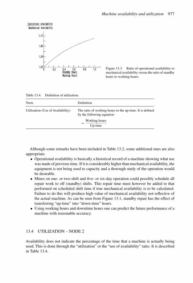
13 MACHINE AVAILABILITY AND UTILIZATION 972
13.1 Introduction 97213.2 Time flow 97313.3 Availability – node 1 97513.4 Utilization – node 2 97713.5 Working efficiency – node 3 97813.6 Job efficiency – node 4 97813.7 Maintenance efficiency – node 5 97913.8 Estimating annual operating time and production capacity 98013.9 Estimating shift operating time and production capacity 98313.10 Annual time flow in rotary drilling 98713.11 Application in prefeasibility work 990
References and bibliography 991Review questions and exercises 992
Index 995

This page intentionally left blankThis page intentionally left blank

Preface to the 3rd Edition
The first edition of Open Pit Mine Planning and Design appeared in 1995. Volume 1, the“Fundamentals”, consisted of six chapters
1. Mine Planning2. Mining Revenues and Costs3. Orebody Description4. Geometrical Considerations5. Pit Limits6. Production Planning
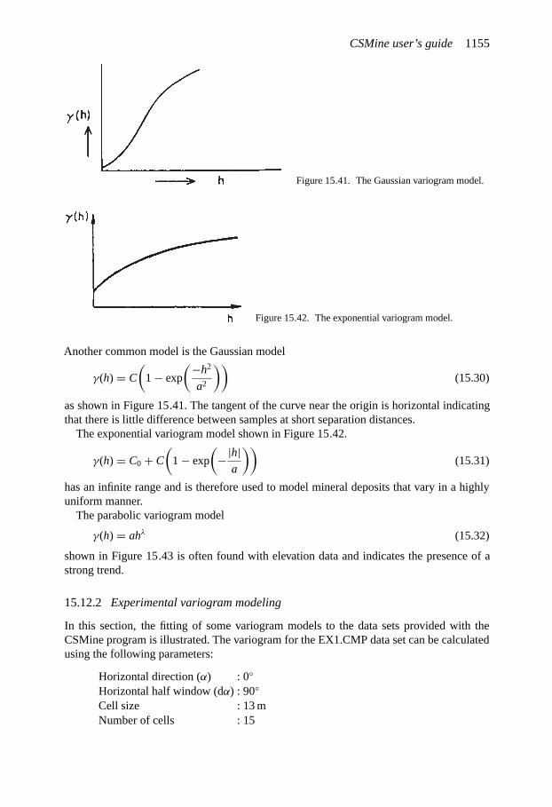
totaling 636 pages. Volume 2, the “CSMine Software Package” was written in support ofthe student- and engineer-friendly CSMine pit generation computer program included on aCD enclosed in a pocket inside the back cover. This volume, which contained six chaptersand 200 pages, consisted of (1) a description of a small copper deposit in Arizona to be usedfor demonstrating and applying the mine planning and design principles, (2) the CSMinetutorial, (3) the CSMine user’s manual, and (4) the VarioC tutorial, user’s manual andreference guide. The VarioC microcomputer program, also included on the CD, was to beused for the statistical analysis of the drill hole data, calculation of experimental variograms,and interactive modeling involving the variogram. The main purpose of the CSMine softwarewas as a learning tool. Students could learn to run it in a very short time and they could thenfocus on the pit design principles rather than on the details of the program. CSMine couldhandle 10,000 blocks which was sufficient to run relatively small problems.
We were very pleased with the response received and it became quite clear that a secondedition was in order. In Volume 1, Chapters 1 and 3 through 6 remained largely the samebut the reference lists were updated. The costs and prices included in Chapter 2 “MiningCosts and Revenues” were updated. Two new chapters were added to Volume 1:
7. Reporting of Mineral Resources and Ore Reserves8. Responsible MiningTo facilitate the use of this book in the classroom, review questions and exercises were
added at the end of Chapters 1 through 8. The “answers” were not, however, provided. Therewere several reasons for this. First, most of the answers could be found by the careful reading,and perhaps re-reading, of the text material. Secondly, for practicing mining engineers, theanswers to the opportunities offered by their operations are seldom provided in advance.The fact that the answers were not given should help introduce the student to the real worldof mining problem solving. Finally, for those students using the book under the guidanceof a professor, some of the questions will offer discussion possibilities. There is no single“right” answer for some of the included exercises.
XV
XVI Open pit mine planning and design: Fundamentals
In Volume 2, the CSMine software included in the first edition was written for theDOS operating system which was current at that time. Although the original programdoes work in the Windows environment, it is not optimum. Furthermore, with the majoradvances in computer power that occurred during the intervening ten-year period, manyimprovements could be incorporated. Of prime importance, however, was to retain the userfriendliness of the original CSMine. Its capabilities were expanded to be able to involve30,000 blocks.
A total of eight drill hole data sets involving three iron properties, two gold properties andthree copper properties were included on the distribution CD. Each of these properties wasdescribed in some detail. It was intended that, when used in conjunction with the CSMinesoftware, these data sets might form the basis for capstone surface mine designs. It hasbeen the experience of the authors when teaching capstone design courses that a significantproblem for the student is obtaining a good drillhole data set. Hopefully the inclusion ofthese data sets has been of some help in this regard.
The second edition was also well received and the time arrived to address the improve-ments to be included in this, the 3rd edition. The structure and fundamentals have withstoodthe passage of time and have been retained. The two-volume presentation has also beenmaintained.
However, for those of you familiar with the earlier editions, you will quickly noticeone major change. A new author, in the form of Randy Martin, has joined the team ofBill Hustrulid and Mark Kuchta in preparing this new offering. Randy is the “Mother andFather” of the very engineer-friendly and widely used MicroMODEL open pit mine designsoftware. As part of the 3rd edition, he has prepared an “academic” version of his softwarepackage. It has all of the features of his commercial version but is limited in application tosix data sets:
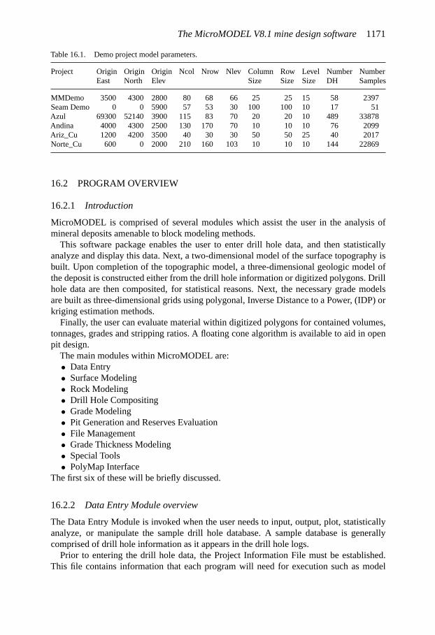
• Ariz_Cu: the same copper deposit used with CSMine (36,000 blocks)• Andina_Cu: a copper deposit from central Chile (1,547,000 blocks)• Azul: a gold deposit from central Chile (668,150 blocks)• MMdemo: a gold deposit in Nevada (359,040 blocks)• Norte_Cu: a copper deposit in northern Chile (3,460,800 blocks)• SeamDemo: a thermal coal deposit in New Mexico (90,630 blocks).Our intention has been to expose the student to more realistic applications once the
fundamentals have been learned via the CSMine software (30,000 block limitation). TheMicroMODEL V8.1 Academic version software is included on the CD together withthe 6 data sets. The accompanying tutorial has been added as Chapter 16. Our idea is thatthe student will begin their computer-aided open pit mine design experience using CSMineand the Ariz_Cu data set and then progress to applying MicroMODEL to the same set withhelp from the tutorial.
The new chapter makeup of Volume 2 is14. The CSMine Tutorial15. CSMine User’s Guide16. The MicroMODEL V8.1 Mine Design Software17. Orebody Case ExamplesVolume 1, “Fundamentals”, has also experienced some noticeable changes. Chapters 1
and 3 through 8 have been retained basically as presented in the second edition. The pricesand costs provided in Chapter 2 have been revised to reflect those appropriate for today(2012). The reference list included at the end of each chapter has been revised. In the earlier

Preface to the 3rd Edition XVII
editions, no real discussion of the basic unit operations was included. This has now beencorrected with the addition of:
9. Blasting10. Rotary Drilling11. Shovel Loading12. Truck Haulage13. Equipment Availability and Utilization
Each chapter has a set of “Review Questions and Exercises”.The authors would like to acknowledge the Canadian Institute of Mining, Metallurgy
and Petroleum (CIM) for permission to include their ‘Estimation of Mineral Resources andMineral Reserves: Best Practices Guidelines’ in Chapter 7. The Australasian Institute ofMining and Metallurgy (AusIMM) was very kind to permit our inclusion of the ‘JORC-2004 Code’ in Chapter 7. The current commodity prices were kindly supplied by Platt’sMetals Week, the Metal Bulletin, Minerals Price Watch, and Skillings Mining Review.The Engineering News-Record graciously allowed the inclusion of their cost indexes. TheCMJ Mining Sourcebook, Equipment Watch (a Penton Media Brand), and InfoMine USAprovided updated costs. Thomas Martin kindly permitted the inclusion of materials from thebook “Surface Mining Equipment”. The authors drew very heavily on the statistics carefullycompiled by the U.S. Department of Labor, the U.S. Bureau of Labor Statistics, and the U.S.Geological Survey. Mining equipment suppliers Atlas Copco, Sandvik Mining, KomatsuAmerica Corporation, Terex Inc., Joy Global (P&H), Siemens Industry, Inc., and VarelInternational have graciously provided us with materials for inclusion in the 3rd edition. Ms.Jane Olivier, Publications Manager, Society for Mining, Metallurgy and Exploration (SME)has graciously allowed inclusion of materials from the 3rd edition, Mining EngineeringHandbook. Otto Schumacher performed a very thorough review of the materials includedin chapters 9 through 13. Last, but not least, Ms. Arlene Chafe provided us access to thepublications of the International Society of Explosive Engineers (ISEE).
The drill hole sets included in Chapter 17 were kindly supplied by Kennecott BarneysCanyon mine, Newmont Mining Corporation, Minnesota Department of Revenue,Minnesota Division of Minerals (lronton Office), Geneva Steel and Codelco.
Finally, we would like to thank those of you who bought the first and second editions ofthis book and have provided useful suggestions for improvement.
The result is what you now hold in your hands. We hope that you will find some thingsof value. In spite of the changes that have taken place in the content of the book over theyears, our basic philosophy has remained the same – to produce a book which will form animportant instrument in the process of learning/teaching about the engineering principlesand application of them involved in the design of open pit mines.
Another important “consistency” with this 3rd edition is the inclusion of the Bingham Piton the cover. Obviously the pit has also changed over the years but this proud lady whichwas first mined as an open pit in 1906 is still a remarkable beauty! Kennecott Utah Coppergenerously provided the beautiful photo of their Bingham Canyon mine for use on the cover.
Important Notice – Please Read
This book has been primarily written for use as a textbook by students studying miningengineering, in general, and surface mining, in particular. The focus has been on presentingthe concepts and principles involved in a logical and easily understood way. In spite of great

XVIII Open pit mine planning and design: Fundamentals
efforts made to avoid the introduction of mistakes both in understanding and presentation,they may have been inadvertently/unintentionally introduced. The authors would be pleasedif you, the reader, would bring such mistakes to their attention so that they may be correctedin subsequent editions.
Neither the authors nor the publisher shall, in any event, be liable for any damages orexpenses, including consequential damages and expenses, resulting from the use of theinformation, methods, or products described in this textbook. Judgments made regardingthe suitability of the techniques, procedures, methods, equations, etc. for any particularapplication are the responsibility of the user, and the user alone. It must be recognized thatthere is still a great deal of ‘art’ in successful mining and hence careful evaluation and testingremains an important part of technique and equipment selection at any particular mine.

About the Authors
William Hustrulid studied Minerals Engineering at theUniversity of Minnesota. After obtaining his Ph.D. degree in 1968,his career has included responsible roles in both mining academiaand in the mining business itself. He has served as Professor ofMining Engineering at the University of Utah and at the ColoradoSchool of Mines and as a Guest Professor at the Technical Universityin Luleå, Sweden. In addition, he has held mining R&D positionsfor companies in the USA, Sweden, and the former Republic ofZaire. He is a Member of the U.S. National Academy of Engineer-ing (NAE) and a Foreign Member of the Swedish Royal Academy of Engineering Sciences(IVA). He currently holds the rank of Professor Emeritus at the University of Utah andmanages Hustrulid Mining Services in Spokane, Washington.
Mark Kuchta studied Mining Engineering at the Colorado Schoolof Mines and received his Ph.D. degree from the TechnicalUniversity in Luleå, Sweden. He has had a wide-ranging careerin the mining business. This has included working as a contractminer in the uranium mines of western Colorado and 10 years ofexperience in various positions with LKAB in northern Sweden. Atpresent, Mark is an Associate Professor of Mining Engineering atthe Colorado School of Mines. He is actively involved in the educa-tion of future mining engineers at both undergraduate and graduatelevels and conducts a very active research program. His professional interests include theuse of high-pressure waterjets for rock scaling applications in underground mines, strategicmine planning, advanced mine production scheduling and the development of user-friendlymine software.
Randall K. “Randy” Martin studied Metallurgical Engineering atthe Colorado School of Mines and later received a Master of Sciencein Mineral Economics from the Colorado School of Mines. He hasover thirty years of experience as a geologic modeler and mineplanner, having worked for Amax Mining, Pincock, Allen & Holt,and Tetratech. Currently he serves as President of R.K. Martin andAssociates, Inc. His company performs consulting services, andalso markets and supports a variety of software packages whichare used in the mining industry. He is the principal author of theMicroMODEL® software included with this textbook.
XIX

This page intentionally left blankThis page intentionally left blank

CHAPTER 1
Mine planning
1.1 INTRODUCTION
1.1.1 The meaning of ore
One of the first things discussed in an Introduction to Mining course and one which studentsmust commit to memory is the definition of ‘ore’. One of the more common definitions(USBM, 1967) is given below:
Ore: A metalliferous mineral, or an aggregate of metalliferous minerals, more or lessmixed with gangue which from the standpoint of the miner can be mined at a profit or, fromthe standpoint of a metallurgist can be treated at a profit.
This standard definition is consistent with the custom of dividing mineral deposits intotwo groups: metallic (ore) and non-metallic. Over the years, the usage of the word ‘ore’ hasbeen expanded by many to include non-metallics as well. The definition of ore suggestedby Banfield (1972) would appear to be more in keeping with the general present day usage.
Ore: A natural aggregate of one or more solid minerals which can be mined, or fromwhich one or more mineral products can be extracted, at a profit.
In this book the following, somewhat simplified, definition will be used:Ore: A natural aggregation of one or more solid minerals that can be mined, processed
and sold at a profit.Although definitions are important to know, it is even more important to know what they
mean. To prevent the reader from simply transferring this definition directly to memorywithout being first processed by the brain, the ‘meaning’ of ore will be expanded upon.
The key concept is ‘extraction leading to a profit’. For engineers, profits can be expressedin simple equation form as
Profits = Revenues − Costs (1.1)
The revenue portion of the equation can be written as
Revenues = Material sold (units) × Price/unit (1.2)
The costs can be similarly expressed as
Costs = Material sold (units) × Cost/unit (1.3)
Combining the equations yields
Profits = Material sold (units) × (Price/unit − Cost/unit) (1.4)
1

2 Open pit mine planning and design: Fundamentals
As has been the case since the early Phoenician traders, the minerals used by modern mancome from deposits scattered around the globe. The price received is more and more beingset by world wide supply and demand. Thus, the price component in the equation is largelydetermined by others. Where the mining engineer can and does enter is in doing somethingabout the unit costs. Although the development of new technology at your property isone answer, new technology easily and quickly spreads around the world and soon alloperations have the ‘new’ technology. Hence to remain profitable over the long term, themining engineer must continually examine and assess smarter and better site specific waysfor reducing costs at the operation. This is done through a better understanding of thedeposit itself and the tools/techniques employed or employable in the extraction process.Cost containment/reduction through efficient, safe and environmentally responsive miningpractices is serious business today and will be even more important in the future withincreasing mining depths and ever more stringent regulations.A failure to keep up is reflectedquite simply by the profit equation as
Profits < 0 (1.5)
This, needless to say, is unfavorable for all concerned (the employees, the company, and thecountry or nation). For the mining engineer (student or practicing) reading this book, thepersonal meaning of ore is
Ore ≡ Profits ≡ Jobs (1.6)
The use of the mathematical equivalence symbol simply says that ‘ore’ is equivalent to ‘prof-its’which is equivalent to ‘jobs’. Hence one important meaning of ‘ore’ to us in the mineralsbusiness is jobs. Probably this simple practical definition is more easily remembered thanthose offered earlier. The remainder of the book is intended to provide the engineer withtools to perform even better in an increasingly competitive world.
1.1.2 Some important definitions
The exploration, development, and production stages of a mineral deposit (Banfield &Havard, 1975) are defined as:
Exploration: The search for a mineral deposit (prospecting) and the subsequentinvestigation of any deposit found until an orebody, if such exists, has been established.
Development: Work done on a mineral deposit, after exploration has disclosed ore insufficient quantity and quality to justify extraction, in order to make the ore available formining.
Production: The mining of ores, and as required, the subsequent processing into productsready for marketing.
It is essential that the various terms used to describe the nature, size and tenor of thedeposit be very carefully selected and then used within the limits of well recognized andaccepted definitions.
Over the years a number of attempts have been made to provide a set of universallyaccepted definitions for the most important terms. These definitions have evolved somewhatas the technology used to investigate and evaluate orebodies has changed. On February 24,1991, the report, ‘A Guide for Reporting Exploration Information, Resources and Reserves’prepared by Working Party No. 79 – ‘Ore Reserves Definition’ of the Society of Mining,Metallurgy and Exploration (SME), was delivered to the SME Board of Directors (SME,

Mine planning 3
1991). This report was subsequently published for discussion. In this section, the ‘Defi-nitions’ and ‘Report Terminology’ portions of their report (SME, 1991) are included. Theinterested reader is encouraged to consult the given reference for the detailed guidelines.The definitions presented are tied closely to the sequential relationship between explorationinformation, resources and reserves shown in Figure 1.1.
With an increase in geological knowledge, the exploration information may becomesufficient to calculate a resource. When economic information increases it may be possibleto convert a portion of the resource to a reserve. The double arrows between reserves andresources in Figure 1.1 indicate that changes due to any number of factors may cause materialto move from one category to another.
DefinitionsExploration information. Information that results from activities designed to locate eco-nomic deposits and to establish the size, composition, shape and grade of these deposits.Exploration methods include geological, geochemical, and geophysical surveys, drill holes,trial pits and surface underground openings.
Resource. A concentration of naturally occurring solid, liquid or gaseous material in or onthe Earth’s crust in such form and amount that economic extraction of a commodity fromthe concentration is currently or potentially feasible. Location, grade, quality, and quantityare known or estimated from specific geological evidence. To reflect varying degrees ofgeological certainty, resources can be subdivided into measured, indicated, and inferred.
– Measured. Quantity is computed from dimensions revealed in outcrops, trenches,workings or drill holes; grade and/or quality are computed from the result of detailed sam-pling. The sites for inspection, sampling and measurement are spaced so closely and thegeological character is so well defined that size, shape, depth and mineral content of theresource are well established.
ExplorationInformation
Reserves
Probable
Proven
Resources
Inferred
Indicated
Measured
Economic, mining, metallurgical, marketingenvironmental, social and governmental
factors may cause material to move betweenresources and reserves
Incr
easi
ng le
vel o
fge
olog
ical
kno
wle
dge
and
conf
iden
ceth
erei
n
Figure 1.1. The relationshipbetween exploration informa-tion, resources and reserves(SME, 1991).

4 Open pit mine planning and design: Fundamentals
– Indicated. Quantity and grade and/or quality are computed from information similar tothat used for measured resources, but the sites for inspection, sampling, and measurementsare farther apart or are otherwise less adequately spaced. The degree of assurance, althoughlower than that for measured resources, is high enough to assume geological continuitybetween points of observation.
– Inferred. Estimates are based on geological evidence and assumed continuity in whichthere is less confidence than for measured and/or indicated resources. Inferred resources mayor may not be supported by samples or measurements but the inference must be supportedby reasonable geo-scientific (geological, geochemical, geophysical, or other) data.
Reserve. A reserve is that part of the resource that meets minimum physical and chemicalcriteria related to the specified mining and production practices, including those for grade,quality, thickness and depth; and can be reasonably assumed to be economically and legallyextracted or produced at the time of determination. The feasibility of the specified miningand production practices must have been demonstrated or can be reasonably assumed on thebasis of tests and measurements. The term reserves need not signify that extraction facilitiesare in place and operative.
The term economic implies that profitable extraction or production under defined invest-ment assumptions has been established or analytically demonstrated. The assumptions mademust be reasonable including assumptions concerning the prices and costs that will prevailduring the life of the project.
The term ‘legally’ does not imply that all permits needed for mining and processing havebeen obtained or that other legal issues have been completely resolved. However, for areserve to exist, there should not be any significant uncertainty concerning issuance of thesepermits or resolution of legal issues.
Reserves relate to resources as follows:– Proven reserve. That part of a measured resource that satisfies the conditions to be
classified as a reserve.– Probable reserve. That part of an indicated resources that satisfies the conditions to be
classified as a reserve.It should be stated whether the reserve estimate is of in-place material or of recoverable
material. Any in-place estimate should be qualified to show the anticipated losses resultingfrom mining methods and beneficiation or preparation.
Reporting terminologyThe following terms should be used for reporting exploration information, resources andreserves:
1. Exploration information. Terms such as ‘deposit’ or ‘mineralization’ are appropriate forreporting exploration information. Terms such as ‘ore,’ ‘reserve,’ and other terms that implythat economic extraction or production has been demonstrated, should not be used.
2. Resource. A resource can be subdivided into three categories:(a) Measured resource;(b) Indicated resource;(c) Inferred resource.
The term ‘resource’ is recommended over the terms ‘mineral resource, identified resource’and ‘in situ resource.’ ‘Resource’ as defined herein includes ‘identified resource,’ butexcludes ‘undiscovered resource’of the United States Bureau of Mines (USBM) and United

Mine planning 5
States Geological Survey (USGS) classification scheme. The ‘undiscovered resource’ clas-sification is used by public planning agencies and is not appropriate for use in commercialventures.
3. Reserve. A reserve can be subdivided into two categories:(a) Probable reserve;(b) Proven reserve.
The term ‘reserve’ is recommended over the terms ‘ore reserve,’ ‘minable reserve’ or‘recoverable reserve.’
The terms ‘measured reserve’ and ‘indicated reserve,’ generally equivalent to ‘provenreserve’ and ‘probable reserve,’ respectively, are not part of this classification scheme andshould not be used. The terms ‘measured,’ ‘indicated’ and ‘inferred’ qualify resources andreflect only differences in geological confidence. The terms ‘proven’ and ‘probable’ qualifyreserves and reflect a high level of economic confidence as well as differences in geologicalconfidence.
The terms ‘possible reserve’ and ‘inferred reserve’ are not part of this classificationscheme. Material described by these terms lacks the requisite degree of assurance to bereported as a reserve.
The term ‘ore’should be used only for material that meets the requirements to be a reserve.It is recommended that proven and probable reserves be reported separately. Where the
term reserve is used without the modifiers proven or probable, it is considered to be the totalof proven and probable reserves.
1.2 MINE DEVELOPMENT PHASES
The mineral supply process is shown diagrammatically in Figure 1.2. As can be seena positive change in the market place creates a new or increased demand for a mineralproduct.
In response to the demand, financial resources are applied in an exploration phase result-ing in the discovery and delineation of deposits. Through increases in price and/or advancesin technology, previously located deposits may become interesting. These deposits mustthen be thoroughly evaluated regarding their economic attractiveness. This evaluation pro-cess will be termed the ‘planning phase’ of a project (Lee, 1984). The conclusion of thisphase will be the preparation of a feasibility report. Based upon this, the decision will bemade as to whether or not to proceed. If the decision is ‘go’, then the development of themine and concentrating facilities is undertaken. This is called the implementation, invest-ment, or design and construction phase. Finally there is the production or operational phaseduring which the mineral is mined and processed. The result is a product to be sold in themarketplace. The entrance of the mining engineer into this process begins at the planningphase and continues through the production phase. Figure 1.3 is a time line showing therelationship of the different phases and their stages.
The implementation phase consists of two stages (Lee, 1984). The design and constructionstage includes the design, procurement and construction activities. Since it is the period ofmajor cash flow for the project, economies generally result by keeping the time frame toa realistic minimum. The second stage is commissioning. This is the trial operation of theindividual components to integrate them into an operating system and ensure their readiness

6 Open pit mine planning and design: Fundamentals
Figure 1.2. Diagrammatic repre-sentation of the mineral supplyprocess (McKenzie, 1980).
Figure 1.3. Relative ability to influence costs (Lee, 1984).
for startup. It is conducted without feedstock or raw materials. Frequently the demands andcosts of the commissioning period are underestimated.
The production phase also has two stages (Lee, 1984). The startup stage commences at themoment that feed is delivered to the plant with the express intention of transforming it intoproduct. Startup normally ends when the quantity and quality of the product is sustainableat the desired level. Operation commences at the end of the startup stage.

Mine planning 7
As can be seen in Figure 1.3, and as indicated by Lee (1984),
the planning phase offers the greatest opportunity to minimize the capital and operating costsof the ultimate project, while maximizing the operability and profitability of the venture. Butthe opposite is also true: no phase of the project contains the potential for instilling technicalor fiscal disaster into a developing project, that is inherent in the planning phase. . . .
At the start of the conceptual study, there is a relatively unlimited ability to influence thecost of the emerging project. As decisions are made, correctly or otherwise, during the bal-ance of the planning phase, the opportunity to influence the cost of the job diminishes rapidly.
The ability to influence the cost of the project diminishes further as more decisions aremade during the design stage. At the end of the construction period there is essentially noopportunity to influence costs.
The remainder of this chapter will focus on the activities conducted within the planningstage.
1.3 AN INITIAL DATA COLLECTION CHECKLIST
In the initial planning stages for any new project there are a great number of factors ofrather diverse types requiring consideration. Some of these factors can be easily addressed,whereas others will require in-depth study. To prevent forgetting factors, checklist are oftenof great value. Included below are the items from a ‘Field Work Program Checklist for NewProperties’developed by Halls (1975). Student engineers will find many of the items on thischecklist of relevance when preparing mine design reports.
Checklist items (Halls, 1975)1. Topography
(a) USGS maps(b) Special aerial or land survey
Establish survey control stationsContour
2. Climatic conditions(a) Altitude(b) Temperatures
ExtremesMonthly averages
(c) PrecipitationAverage annual precipitationAverage monthly rainfallAverage monthly snowfallRun-off
NormalFlood
Slides – snow and mud(d) Wind
Maximum recordedPrevailing directionHurricanes, tornados, cyclones, etc.

8 Open pit mine planning and design: Fundamentals
(e) HumidityEffect on installations, i.e. electrical motors, etc.
(f) Dust(g) Fog and cloud conditions
3. Water – potable and process(a) Sources
StreamsLakesWells
(b) AvailabilityOwnershipWater rightsCost
(c) QuantitiesMonthly availabilityFlow ratesDrought or flood conditionsPossible dam locations
(d) QualityPresent samplePossibility of quality change in upstream source waterEffect of contamination on downstream users
(e) Sewage disposal method4. Geologic structure
(a) Within mine area(b) Surrounding areas(c) Dam locations(d) Earthquakes(e) Effect on pit slopes
Maximum predicted slopes(f) Estimate on foundation conditions
5. Mine water as determined by prospect holes(a) Depth(b) Quantity(c) Method of drainage
6. Surface(a) Vegetation
TypeMethod of clearingLocal costs for clearing
(b) Unusual conditionsExtra heavy timber growthMuskegLakesStream diversionsGravel deposits

Mine planning 9
7. Rock type – overburden and ore(a) Submit sample for drillability test(b) Observe fragmentation features
HardnessDegree of weatheringCleavage and fracture planesSuitability for road surface
8. Locations for concentrator – factors to consider for optimumlocation(a) Mine location
Haul uphill or downhill(b) Site preparation
Amount of cut and/or fill(c) Process water
Gravity flow or pumping(d) Tailings disposal
Gravity flow or pumping(e) Maintenance facilities
Location9. Tailings pond area
(a) Location of pipeline length and discharge elevations(b) Enclosing features
NaturalDams or dikesLakes
(c) Pond overflowEffect of water pollution on downstream usersPossibility for reclaiming water
(d) Tailings dustIts effect on the area
10. Roads(a) Obtain area road maps(b) Additional road information
WidthsSurfacingMaximum load limitsSeasonal load limitsSeasonal accessOther limits or restrictionsMaintained by county, state, etc.
(c) Access roads to be constructed by company (factors considered)DistanceProfileCut and fillBridges, culvertsTerrain and soil conditions

10 Open pit mine planning and design: Fundamentals
11. Power(a) Availability
KilovoltsDistanceRates and length of contract
(b) Power lines to siteWho buildsWho maintainsRight-of-way requirements
(c) Substation location(d) Possibility of power generation at or near site
12. Smelting(a) Availability(b) Method of shipping concentrate(c) Rates(d) If company on site smelting – effect of smelter gases(e) Concentrate freight rates(f) Railroads and dock facility
13. Land ownership(a) Present owners(b) Present usage(c) Price of land(d) Types of options, leases and royalties expected
14. Government(a) Political climate
Favorable or unfavorable to miningPast reactions in the area to mining
(b) Special mining laws(c) Local mining restrictions
15. Economic climate(a) Principal industries(b) Availability of labor and normal work schedules(c) Wage scales(d) Tax structure(e) Availability of goods and services
HousingStoresRecreationMedical facilities and unusual local diseaseHospitalSchools
(f) Material costs and/or availabilityFuel oilConcreteGravelBorrow material for dams

Mine planning 11
(g) PurchasingDuties
16. Waste dump location(a) Haul distance(b) Haul profile(c) Amenable to future leaching operation
17. Accessibility of principal town to outside(a) Methods of transportation available(b) Reliability of transportation available(c) Communications
18. Methods of obtaining information(a) Past records (i.e. government sources)(b) Maintain measuring and recording devices(c) Collect samples(d) Field observations and measurements(e) Field surveys(f) Make preliminary plant layouts(g) Check courthouse records for land information(h) Check local laws and ordinances for applicable legislation(i) Personal inquiries and observation on economic and political climates(j) Maps(k) Make cost inquiries(l) Make material availability inquiries
(m) Make utility availability inquiries
1.4 THE PLANNING PHASE
In preparing this section the authors have drawn heavily on material originally presented inpapers by Lee (1984) and Taylor (1977). The permission by the authors and their publisher,The Northwest Mining Association, to include this material is gratefully acknowledged.
1.4.1 Introduction
The planning phase commonly involves three stages of study (Lee, 1984).
Stage 1: Conceptual studyA conceptual (or preliminary valuation) study represents the transformation of a projectidea into a broad investment proposition, by using comparative methods of scope definitionand cost estimating techniques to identify a potential investment opportunity. Capital andoperating costs are usually approximate ratio estimates using historical data. It is intendedprimarily to highlight the principal investment aspects of a possible mining proposition. Thepreparation of such a study is normally the work of one or two engineers. The findings arereported as a preliminary valuation.
Stage 2: Preliminary or pre-feasibility studyA preliminary study is an intermediate-level exercise, normally not suitable for an investmentdecision. It has the objectives of determining whether the project concept justifies a detailed

12 Open pit mine planning and design: Fundamentals
analysis by a feasibility study, and whether any aspects of the project are critical to itsviability and necessitate in-depth investigation through functional or support studies.
A preliminary study should be viewed as an intermediate stage between a relativelyinexpensive conceptual study and a relatively expensive feasibility study. Some are doneby a two or three man team who have access to consultants in various fields others may bemulti-group efforts.
Stage 3: Feasibility studyThe feasibility study provides a definitive technical, environmental and commercial basefor an investment decision. It uses iterative processes to optimize all critical elements ofthe project. It identifies the production capacity, technology, investment and productioncosts, sales revenues, and return on investment. Normally it defines the scope of workunequivocally, and serves as a base-line document for advancement of the project throughsubsequent phases.
These latter two stages will now be described in more detail.
1.4.2 The content of an intermediate valuation report
The important sections of an intermediate valuation report (Taylor, 1977) are:– Aim;– Technical concept;– Findings;– Ore tonnage and grade;– Mining and production schedule;– Capital cost estimate;– Operating cost estimate;– Revenue estimate;– Taxes and financing;– Cash flow tables.
The degree of detail depends on the quantity and quality of information. Table 1.1 outlinesthe contents of the different sections.
1.4.3 The content of the feasibility report
The essential functions of the feasibility report are given in Table 1.2.Due to the great importance of this report it is necessary to include all detailed information
that supports a general understanding and appraisal of the project or the reasons for selectingparticular processes, equipment or courses of action. The contents of the feasibility reportare outlined in Table 1.3.
The two important requirements for both valuation and feasibility reports are:1. Reports must be easy to read, and their information must be easily accessible.2. Parts of the reports need to be read and understood by non-technical people.
According to Taylor (1977):
There is much merit in a layered or pyramid presentation in which the entire body ofinformation is assembled and retained in three distinct layers.
Layer 1. Detailed background information neatly assembled in readable form and ade-quately indexed, but retained in the company’s office for reference and not included in thefeasibility report.

Mine planning 13
Layer 2. Factual information about the project, precisely what is proposed to be doneabout it, and what the technical, physical and financial results are expected to be.
Layer 3. A comprehensive but reasonably short summary report, issued preferably as aseparate volume.
The feasibility report itself then comprises only the second and third layers. While every-thing may legitimately be grouped into a single volume, the use of smaller separated volumesmakes for easier reading and for more flexible forms of binding. Feasibility reports alwaysneed to be reviewed by experts in various specialities. The use of several smaller volumesmakes this easier, and minimizes the total number of copies needed.
Table 1.1. The content of an intermediate valuation report (Taylor, 1977).
Aim: States briefly what knowledge is being sought about the property, and why, for guidance inexploration spending, for joint venture negotiations, for major feasibility study spending, etc. Sources ofinformation are also conveniently listed.
Concept: Describes very briefly where the property is located, what is proposed or assumed to be done inthe course of production, how this may be achieved, and what is to be done with the products.
Findings: Comprise a summary, preferably in sequential and mainly tabular forms, of the important figuresand observations from all the remaining sections. This section may equally be termed Conclusions,though this title invites a danger of straying into recommendations which should not be offered unlessspecially requested.
Any cautions or reservations the authors care to make should be incorporated in one of the first threesections. The general aim is that the non-technical or less-technical reader should be adequately informedabout the property by the time he has read the end of Findings.
Ore tonnage and grade: Gives brief notes on geology and structure, if applicable, and on the drilling andsampling accomplished. Tonnages and grades, both geological and minable and possibly at variouscut-off grades, are given in tabular form with an accompanying statement on their status and reliability.
Mining and production schedule: Tabulates the mining program (including preproduction work), the millingprogram, any expansions or capacity changes, the recoveries and product qualities (concentrate grades),and outputs of products.
Capital cost estimate: Tabulates the cost to bring the property to production from the time of writingincluding the costs of further exploration, research and studies. Any prereport costs, being sunk, may benoted separately.An estimate of postproduction capital expenditures is also needed. This item, because it consists largelyof imponderables, tends to be underestimated even in detailed feasibilities studies.
Operating cost estimate: Tabulates the cash costs of mining, milling, other treatment, ancillary services,administration, etc. Depreciation is not a cash cost, and is handled separately in cash flow calculations.Postmine treatment and realization costs are most conveniently regarded as deductions from revenues.
Revenue estimate: Records the metal or product prices used, states the realization terms and costs, andcalculates the net smelter return or net price at the deemed point of disposal. The latter is usually takento be the point at which the product leaves the mine’s plant and is handed over to a common carrier.Application of these net prices to the outputs determined in the production schedule yields a schedule ofannual revenues.
Financing and tax data: State what financing assumptions have been made, all equity, all debt or somespecified mixture, together with the interest and repayment terms of loans. A statement on the taxregime specifies tax holidays (if any), depreciation and tax rates, (actual or assumed) and any special
(Continued)

14 Open pit mine planning and design: Fundamentals
Table 1.1. (Continued).
features. Many countries, particularly those with federal constitutions, impose multiple levels oftaxation by various authorities, but a condensation or simplification of formulae may suffice for earlystudies without involving significant loss of accuracy.
Cash flow schedules: Present (if information permits) one or more year-by-year projections of cashmovements in and out of the project. These tabulations are very informative, particularly because theirformat is almost uniformly standardized. They may be compiled for the indicated life of the project or,in very early studies, for some arbitrary shorter period.Figures must also be totalled and summarized. Depending on company practice and instructions,investment indicators such as internal rate of return, debt payback time, or cash flow after payback maybe displayed.
Table 1.2. The essential functions of the feasibility report (Taylor, 1977).
1. To provide a comprehensive framework of established and detailed facts concerning the mineralproject.
2. To present an appropriate scheme of exploitation with designs and equipment lists taken to a degreeof detail sufficient for accurate prediction of costs and results.
3. To indicate to the project’s owners and other interested parties the likely profitability of investmentin the project if equipped and operated as the report specifies.
4. To provide this information in a form intelligible to the owner and suitable for presentation toprospective partners or to sources of finance.
Table 1.3. The content of a feasibility study (Taylor, 1977).
General:– Topography, climate, population, access, services.– Suitable sites for plant, dumps, towns, etc.
Geological (field):– Geological study of structure, mineralization and possibly of genesis.– Sampling by drilling or tunnelling or both.– Bulk sampling for checking and for metallurgical testing.– Extent of leached or oxidized areas (frequently found to be underestimated).– Assaying and recording of data, including check assaying, rock properties, strength and stability.– Closer drilling of areas scheduled for the start of mining.– Geophysics and indication of the likely ultimate limits of mineralization, including proof of
non-mineralization of plan and dump areas.– Sources of water and of construction materials.
Geological and mining (office):– Checking, correcting and coding of data for computer input.– Manual calculations of ore tonnages and grades.– Assay compositing and statistical analysis.– Computation of mineral inventory (geological reserves) and minable reserves, segregated as needed
by orebody, by ore type, by elevation or bench, and by grade categories.– Computation of associated waste rock.– Derivation of the economic factors used in the determination of minable reserves.
Mining:– Open pit layouts and plans.– Determination of preproduction mining or development requirements.– Estimation of waste rock dilution and ore losses.
(Continued)

Mine planning 15
Table 1.3. (Continued).
– Production and stripping schedules, in detail for the first few years but averaged thereafter, andspecifying important changes in ore types if these occur.
– Waste mining and waste disposal.– Labor and equipment requirements and cost, and an appropriate replacement schedule for the major
equipment.
Metallurgy (research):– Bench testing of samples from drill cores.– Selection of type and stages of the extraction process.– Small scale pilot plant testing of composited or bulk samples followed by larger scale pilot mill
operation over a period of months should this work appear necessary.– Specification of degree of processing, and nature and quality of products.– Provision of samples of the product.– Estimating the effects of ore type or head grade variations upon recovery and product quality.
Metallurgy (design):– The treatment concept in considerable detail, with flowsheets and calculation of quantities flowing.– Specification of recovery and of product grade.– General siting and layout of plant with drawings if necessary.
Ancillary services and requirements:– Access, transport, power, water, fuel and communications.– Workshops, offices, changehouse, laboratories, sundry buildings and equipment.– Labor structure and strength.– Housing and transport of employees.– Other social requirements.
Capital cost estimation:– Develop the mine and plant concepts and make all necessary drawings.– Calculate or estimate the equipment list and all important quantities (of excavation, concrete, building
area and volume, pipework, etc.).– Determine a provisional construction schedule.– Obtain quotes of the direct cost of items of machinery, establish the costs of materials and services,
and of labor and installation.– Determine the various and very substantial indirect costs, which include freight and taxes on equipment
(may be included in directs), contractors’ camps and overheads plus equipment rental, labor punitive andfringe costs, the owner’s field office, supervision and travel, purchasing and design costs, licenses, fees,customs duties and sales taxes.
– Warehouse inventories.– A contingency allowance for unforeseen adverse happenings and for unestimated small requirements
that may arise.– Operating capital sufficient to pay for running the mine until the first revenue is received.– Financing costs and, if applicable, preproduction interest on borrowed money.
A separate exercise is to forecast the major replacements and the accompanying provisions forpostproduction capital spending. Adequate allowance needs to be made for small requirements that, thoughunforeseeable, always arise in significant amounts.
Operating cost estimation:– Define the labor strength, basic pay rates, fringe costs.– Establish the quantities of important measurable supplies to be consumed – power, explosives, fuel,
grinding steel, reagents, etc. – and their unit costs.– Determine the hourly operating and maintenance costs for mobile equipment plus fair performance
factors.– Estimate the fixed administration costs and other overheads plus the irrecoverable elements of
townsite and social costs.
(Continued)

16 Open pit mine planning and design: Fundamentals
Table 1.3. (Continued).
Only cash costs are used thus excluding depreciation charges that must be accounted for elsewhere. As forearlier studies, post-mine costs for further treatment and for selling the product are best regarded asdeductions from the gross revenue.
Marketing:– Product specifications, transport, marketing regulations or restrictions.– Market analysis and forecast of future prices.– Likely purchasers.– Costs for freight, further treatment and sales.– Draft sales terms, preferably with a letter of intent.– Merits of direct purchase as against toll treatment.– Contract duration, provisions for amendment or cost escalation.– Requirements for sampling, assaying and umpiring.
The existence of a market contract or firm letter of intent is usually an important prerequisite to the loanfinancing of a new mine.
Rights, ownership and legal matters:– Mineral rights and tenure.– Mining rights (if separated from mineral rights).– Rents and royalties.– Property acquisitions or securement by option or otherwise.– Surface rights to land, water, rights-of-way, etc.– Licenses and permits for construction as well as operation.– Employment laws for local and expatriate employees separately if applicable.– Agreements between partners in the enterprise.– Legal features of tax, currency exchange and financial matters.– Company incorporation.
Financial and tax matters:– Suggested organization of the enterprise, as corporation, joint-venture or partnership.– Financing and obligations, particularly relating to interest and repayment on debt.– Foreign exchange and reconversion rights, if applicable.– Study of tax authorities and regimes, whether single or multiple.– Depreciation allowances and tax rates.– Tax concessions and the negotiating procedure for them.– Appropriation and division of distributable profits.
Environmental effects:– Environmental study and report; the need for pollution or related permits, the requirements during
construction and during operation.– Prescribed reports to government authorities, plans for restoration of the area after mining ceases.
Revenue and profit analysis:– The mine and mill production schedules and the year-by-year output of products.– Net revenue at the mine (at various product prices if desired) after deduction of transport, treatment
and other realization charges.– Calculation of annual costs from the production schedules and from unit operating costs derived
previously.– Calculation of complete cash flow schedules with depreciation, taxes, etc. for some appropriate
number of years – individually for at least 10 years and grouped thereafter.– Presentation of totals and summaries of results.– Derived figures (rate of return, payback, profit split, etc.) as specified by owner or client.– Assessment of sensitivity to price changes and generally to variation in important input
elements.

Mine planning 17
1.5 PLANNING COSTS
The cost of these studies (Lee, 1984) varies substantially, depending upon the size andnature of the project, the type of study being undertaken, the number of alternatives tobe investigated, and numerous other factors. However, the order of magnitude cost of thetechnical portion of studies, excluding such owner’s cost items as exploration drilling, spe-cial grinding or metallurgical tests, environmental and permitting studies, or other supportstudies, is commonly expressed as a percentage of the capital cost of the project:
Conceptual study: 0.1 to 0.3 percent
Preliminary study: 0.2 to 0.8 percent
Feasibility study: 0.5 to 1.5 percent
1.6 ACCURACY OF ESTIMATES
The material presented in this section has been largely extracted from the paper ‘MineValuation and Feasibility Studies’ presented by Taylor (1977).
1.6.1 Tonnage and grade
At feasibility, by reason of multiple sampling and numerous checks, the average mininggrade of some declared tonnage is likely to be known within acceptable limits, say ±5%,and verified by standard statistical methods. Although the ultimate tonnage of ore maybe known for open pit mines if exploration drilling from surface penetrates deeper thanthe practical mining limit, in practice, the ultimate tonnage of many deposits is nebulousbecause it depends on cost-price relationships late in the project life. By the discount effectsin present value theory, late life tonnage is not economically significant at the feasibilitystage. Its significance will grow steadily with time once production has begun. It is notcritical that the total possible tonnage be known at the outset. What is more important is thatthe grade and quality factors of the first few years of operation be known with assurance.
Two standards of importance can be defined for most large open pit mines:1. A minimum ore reserve equal to that required for all the years that the cash flows are
projected in the feasibility report must be known with accuracy and confidence.2. An ultimate tonnage potential, projected generously and optimistically, should be
calculated so as to define the area adversely affected by mining and within which dumpsand plant buildings must not encroach.
1.6.2 Performance
This reduces to two items – throughput and recovery. Open pit mining units have wellestablished performance rates that can usually be achieved if the work is correctly organizedand the associated items (i.e. shovels and trucks) are suitably matched. Performance suffersif advance work (waste stripping in a pit) is inadequate. Care must be taken that these tasksare adequately scheduled and provided for in the feasibility study.
The throughput of a concentrator tends to be limited at either the fine crushing stage or thegrinding stages. The principles of milling design are well established, but their application

18 Open pit mine planning and design: Fundamentals
requires accurate knowledge of the ore’s hardness and grindability. These qualities musttherefore receive careful attention in the prefeasibility test work. Concentrator performanceis part of a three way relationship involving the fineness of grind, recovery, and the gradeof concentrate or product. Very similar relations may exist in metallurgical plants of othertypes. Again, accuracy can result only from adequate test-work.
1.6.3 Costs
Some cost items, notably in the operating cost field, differ little from mine to mine and arereliably known in detail. Others may be unique or otherwise difficult to estimate. Generally,accuracy in capital or operating cost estimating goes back to accuracy in quantities, reliablequotes or unit prices, and adequate provision for indirect or overhead items. The latter tend toform an ever increasing burden. For this reason, they should also be itemized and estimateddirectly whenever possible, and not be concealed in or allocated into other direct cost items.
Contingency allowance is an allowance for possible over expenditures contingent uponunforeseen happenings such as a strike or time delaying accident during construction, poorplant foundation conditions, or severe weather problems. To some extent the contingencyallowance inevitably allows for certain small expenditures always known to arise but notforeseeable nor estimable in detail. Caution is needed here. The contingency allowance isnot an allowance for bad or inadequate estimating, and it should never be interpreted in thatmanner.
The accuracy of capital and operating cost estimates increases as the project advancesfrom conceptual to preliminary to feasibility stage. Normally acceptable ranges of accuracyare considered to be (Lee, 1984):
Conceptual study: ±30 percent
Preliminary study: ±20 percent
Feasibility study: ±10 percent
It was noted earlier that the scope of work in the conceptual and preliminary studies is notoptimized. The cost estimate is suitable for decision purposes, to advance the project to thenext stage, or to abort and minimize losses.
1.6.4 Price and revenue
The revenue over a mine’s life is the largest single category of money. It has to pay foreverything, including repayment of the original investment money. Because revenue is thebiggest base, measures of the mine’s economic merit are more sensitive to changes in revenuethan to changes of similar ratio in any of the expenditure items.
Revenue is governed by grade, throughput, recovery, and metal or product price. Of these,price is: (a) by far the most difficult to estimate and (b) the one quantity largely outside theestimator’s control. Even ignoring inflation, selling prices are widely variable with time.Except for certain controlled commodities, they tend to follow a cyclic pattern.
The market departments of major metal mining corporations are well informed onsupply/demand relationships and metal price movements. They can usually provide fore-casts of average metal prices in present value dollars, both probable and conservative, thelatter being with 80% probability or better. Ideally, even at the conservative product price,the proposed project should still display at least the lowest acceptable level of profitability.

Mine planning 19
1.7 FEASIBILITY STUDY PREPARATION
The feasibility study is a major undertaking involving many people and a variety ofspecialized skills. There are two basic ways through which it is accomplished.
1. The mining company itself organizes the study and assembles the feasibility report.Various parts or tasks are assigned to outside consultants.
2. The feasibility work is delegated to one or more engineering companies.Contained on the following pages is an eleven step methodology outlining the planning(Steps 1–4) organizing (Steps 5–10) and execution (Step 11) steps which might be used inconducting a feasibility study. It has been developed by Lee (1984, 1991).
Phase A. PlanningStep 1: Establish a steering committee. A steering committee consisting of managers andother individuals of wide experience and responsibility would be formed to overview andevaluate the direction and viability of the feasibility study team. One such steering committeemight be the following:
– Vice-President (Chairman);– General Manager, mining operations;– Vice-President, finance;– Chief Geologist, exploration;– Vice-President, technical services;– Consultant(s).
Step 2: Establish a project study team. The criteria for selection of the study team memberswould emphasize these qualities:
– Competent in their respective fields.– Considerable experience with mining operations.– Complementary technical abilities.– Compatible personalities – strong interpersonal qualities.– Commitment to be available through the implementation phase, should the prospect
be viable.The team members might be:– Project Manager;– Area Supervisor, mining;– Area Supervisor, beneficiation;– Area Supervisor, ancillaries.
Step 3: Develop a work breakdown structure. The Work Breakdown Structure (WBS) isdefined by the American Association of Cost Engineers (AACE) as:
a product-oriented family tree division of hardware, software, facilities and other itemswhich organizes, defines and displays all of the work to be performed in accomplishing theproject objectives.
The WBS is a functional breakdown of all elements of work on a project, on a geographicaland/or process basis. It is a hierarchy of work packages, or products, on a work area basis.The WBS is project-unique, reflecting the axiom that every project is a unique event.
A WBS is a simple common-sense procedure which systematically reviews the full scopeof a project (or study) and breaks it down into logical packages of work. The primary

20 Open pit mine planning and design: Fundamentals
challenge is normally one of perspective. It is imperative that the entire project be visualizedas a sum of many parts, any one of which could be designed, scheduled, constructed, andpriced as a single mini-project.
There are a number of categories which can be used to construct a work breakdownstructure. These include:
(1) Components of the product;(2) Functions;(3) Organizational units;(4) Geographical areas;(5) Cost accounts;(6) Time phases;(7) Configuration characteristics;(8) Deliverables;(9) Responsible persons;
(10) Subpurposes.It is not a rigid system. WBS categories can be used in any sequence desired, includingusing the same category several times. A sample WBS is shown in Figures 1.4 and 1.5.
An alternative to this is the Work Classification Structure (WCS). This commodity-basedclassification of goods and services is commonly used by construction contractors andconsulting engineering firms as the primary cost-collection system. The specific intent ofthe WCS is to provide a consistent reference system for storage, comparison and evaluationof technical, man-hour and cost data from work area to work area within a project; andfrom project to project; and from country to country. The WCS may have different names indifferent organizations, but it is the ‘original’ costing system. It is the basis for virtually allof the estimating manuals and handbooks which identify unit costs for commodities suchas concrete, or piping, or road construction, or equipment installation. The WCS provides acommodity based method to estimate and control costs. The key to the success of the WCSsystem within an organization is the absolute consistency with which it is used.
The WBS is of primary interest to owners and project managers – both of whom areinterested in tracking cost and schedule on a work area basis. TheWCS is primarily of interestto construction contractors and engineering consultants, who measure actual performanceagainst forecast performance on a commodity basis.
Professional project managers and cost engineers normally use cost coding systems whichencode both the commodity and the work package. This allows them to evaluate job-to-dateperformance, then forecast cost or productivity trends for the balance of the project.
Step 4: Develop an action plan for the study. An action plan in its simplest form, is just alogical (logic-oriented) time-bar plan listing all of the activities to be studied. Figure 1.6is one example of such a time-bar graph. A more general action plan would have thesecharacteristics:
1. Purpose: the action plan serves as a control document during the execution of thefeasibility study. It functions as a master reference, against which change can be measuredand resolved. It provides a visual communication of the logic and progress of the study.
2. Methodology: it may be possible for one person, working in isolation, to developan action plan. However, it is substantially more desirable to have the project studyteam develop their plan on a participative, interactive basis. (Texas Instruments’ PatrickHaggerty insisted that ‘those who implement plans must make the plans’). This interaction

Mine
planning21Figure 1.4. Typical work breakdown structure (WBS) directs for an open pit mining project (Lee, 1991).

22 Open pit mine planning and design: Fundamentals
Figure 1.5. Typical work breakdown structure (WBS) indirects for an open pit mining project (Lee, 1991).
fosters understanding and appreciation of mutual requirements and objectives; even moreimportantly, it develops a shared commitment.
3. Format: a simple master time-bar schedule would be produced, displaying the studyactivities in a logic-oriented fashion. Brief titles and a reference number would be attachedto each activity. For a simple in-house job, an operating company would probably stop atthis point. However, for a major study on a new mining operation, the activity referencenumbers and titles would be carried into a separate action plan booklet. Each activity wouldbe described briefly, and a budget attached to it.
4. WBS reference: the most convenient way to organize these activities is by referen-cing them to the first and second levels of the WBS.
5. Number of activities: the practical limitation on the number of individual study activi-ties would be of the order of one hundred.

Mine planning 23
Figure 1.6. Bar chart representation for a mine feasibility/decision-making sequence (McKelvey, 1984).
Phase B. OrganizingStep 5: Identify additional resource requirements. While developing a comprehensive actionplan, needs for additional resources normally become apparent.
Step 6: Identify secondary project team members.
Step 7: Develop organization chart and responsibilities. There are a number of ways toorganize a project study team for a large study. A separate task force can be established byremoving personnel from existing jobs and developing a project-oriented hierarchy, militarystyle. This can work effectively, but can discourage broad participation in the evolution ofthe project. In a large company, a matrix system can be used very successfully, if used verycarefully and with understanding. The management of a matrix organization is based on themanagement of intentional conflict; it works exceedingly well in a positive environment,and is an unequivocal disaster in an unfavorable environment.
Step 8: Develop second-level plans and schedules. Using the master time-bar, the actionplan and the WBS as primary references, the enlarged project study team develops second-level plans and schedules, thus establishing their objectives and commitments for the balanceof the study. These schedules are oriented on an area-by-area basis, with the primary teammembers providing the leadership for each area.
Step 9: Identify special expertise required. The project study team after reviewing their plan,with the additional information developed during Step 8, may identify a number of areas of

24 Open pit mine planning and design: Fundamentals
the job which require special expertise. Such items may be packaged as separate RequestsFor Proposals (RFP’s), and forwarded to pre-screened consultants on an invitation basis.The scope of work in each RFP should be clearly identified, along with the objectives forthe work. A separate section provides explicit comments on the criteria for selection of thesuccessful bidder; this provides the bidder with the opportunity to deliver proposals whichcan be weighted in the directions indicated by the project team.
Step 10: Evaluate and select consultants. Evaluation of the consultant’s bids should bethorough, objective, and fair. The evaluations and decisions are made by the use of spreadsheets which compare each bidder’s capability to satisfy each of the objectives for the workas identified in the RFP. The objectives should be pre-weighted to remove bias from theselection process.
Phase C. ExecutionStep 11: Execute, monitor, control. With the project study team fully mobilized and withthe specialist consultants engaged and actively executing well-defined contracts, the primarychallenge to the project manager is to ensure that the study stays on track.
A number of management and reporting systems and forms may be utilized, but thebase-line reference for each system and report is the scope of work, schedule and cost foreach activity identified in the action plan. The status-line is added to the schedule on abi-weekly basis, and corrections and modifications made as indicated, to keep the work ontrack.
1.8 CRITICAL PATH REPRESENTATION
Figure 1.7 is an example of a network chart which has been presented by Taylor (1977) fora medium sized, open pit base metal mine. Each box on the chart contains:
– activity number,– activity title,– responsibility (this should be a person/head of section who would carry the responsi-
bility for budget and for progress reports),– starting date,– completion date,– task duration.The activities, sequential relationships and critical/near critical paths can be easily seen.Figure 1.8 is the branch showing the basic mining related activities. This progression will
be followed through the remainder of the book.
1.9 MINE RECLAMATION
1.9.1 Introduction
In the past, reclamation was something to be considered at the end of mine operations andnot in the planning stage. Today, in many countries at least, there will be no mine with-out first thoroughly and satisfactorily addressing the environmental aspects of the proposed

Mine planning 25
project. Although the subject of mine reclamation is much too large to be covered in thisbrief chapter, some of the factors requiring planning consideration will be discussed. Inthe western United States, a considerable amount of mineral development takes place onfederal and Indian lands. The Bureau of Land Management (BLM) of the U.S. Depart-ment of the Interior has developed the Solid Minerals Reclamation Handbook (BLM, 1992)with the objective being ‘to provide the user with clear guidance which highlights a log-ical sequence for managing the reclamation process and a summary of key reclamationprinciples.’
The remaining sections of this chapter have been extracted from the handbook. Althoughthey only pertain directly to those lands under BLM supervision, the concepts have moregeneral application as well. Permission from the BLM to include this material is gratefullyacknowledged.
1.9.2 Multiple-use management
Multiple-use management is the central concept in the Federal Land Policy and ManagementAct (FLPMA) of 1976. FLPMA mandates that ‘the public lands be managed in a mannerthat will protect the quality of scientific, scenic, historical, ecological, environmental, airand atmospheric, water resource and archeological values.’ Multiple-use management isdefined in FLPMA (43 USC 1702(c)) and in regulations (43 CFR 1601.0-5(f)) as, in part,the ‘harmonious and coordinated management of the various resources without permanentimpairment of the productivity of the lands and the quality of the environment with con-sideration being given to the relative values of the resources and not necessarily to thecombination of uses that will give the greatest economic return or the greatest unit output.’In addition, FLPMA mandates that activities be conducted so as to prevent ‘unnecessary orundue degradation of the lands’ (43 USC 1732 (b)).
The Mining and Minerals Policy Act of 1970 (30 USC 21(a)) established the policy forthe federal government relating to mining and mineral development. The Act states that it ispolicy to encourage the development of ‘economically sound and stable domestic mining,minerals, metal and mineral reclamation industries.’ The Act also states, however, that thegovernment should also promote the ‘development of methods for the disposal, control, andreclamation of mineral waste products, and the reclamation of mined land, so as to lessenany adverse impact of mineral extraction and processing upon the physical environment thatmay result from mining or mineral activities.’
In accordance with the National Environmental Policy Act (NEPA), an environmentaldocument will be prepared for those mineral actions which propose surface disturbance.The requirements and mitigation measures recommended in an Environmental Assess-ment (ERA) or Environmental Impact Statement (EIS) shall be made a part of thereclamation plan.
It is a statutory mandate that BLM ensure that reclamation and closure of mineral opera-tions be completed in an environmentally sound manner. The BLM’s long-term reclamationgoals are to shape, stabilize, revegetate, or otherwise treat disturbed areas in order to providea self-sustaining, safe, and stable condition that provides a productive use of the land whichconforms to the approved land-use plan for the area. The short-term reclamation goals are tostabilize disturbed areas and to protect both disturbed and adjacent undisturbed areas fromunnecessary or undue degradation.

26 Open pit mine planning and design: Fundamentals
2. Mining
1. Property geology
3. Marketing
4. Metallurgy
5. Plant
6. Water
7. Electrical
91
81
141
141
8. Tailing
9. Mine dumps
10. Railroad siding
11. Townsite and roads
12. Legal matters
13. Finance and accounting
14. Environmental effects
1 UnderGR.survey
Fieldgeologists
3/24
5/25
9
2Geolog.mapping
Fieldgeologists
3/3
5/4
9
5/25
5/5
4Prel.geol.
reportExpl.dept.
3
7Drillingpriority
Expl.dept.
5/28
6/1
1
8AssayDDH.core
Researchlab.
4/28
7/13
11
22Modify
comp.prog.computersection
6/16
7/13
4
9Ore DRLG.
stage 38Field
geologists
6/2
6/29
4
33Smelter
schedulesMarketingmanager
6/30
7/13
4
54Drawing& plans
Eng.consultant
7/28
8/24
4
55Village
relocationLocaloffice
6/30
7/27
2
52Plant
conceptsProject
engineers
6/2
7/27
8
51Option
plantsiteLocaloffice
3/3
4/27
8
53Purchasing
inform.Purchasingmanager
6/2
6/29
4
81Drill
tailingarea
Fieldgeologists
6/2
2
6/15
91Drill
dumparea
Fieldgeologists
6/2
2
6/15
62Acquire
well sitesLocaloffice
6/30
8/10
6
61Drillwells
Fieldgeologists
3/24
5/25
9
60Option
well sitesLocaloffice
3/3
3/16
2
6/30
8/10
6
82Securetailingarea
Localoffice
92Securedumparea
Localoffice
6/30
8/10
6
6/30
8/10
6
102Securerailroadsiding
Localoffice101
Investigaterailroadsiding
Localoffice
6/2
6/15
2
112Roadstudy
Localoffice
6/9
6/22
2111
Securetownsite
Localoffice
5/5
6/1
4
132Ruling onfee taxes
Localoffice
5/5
7/27
12
5/5
7/27
12
133Fiscal
agreementLocaloffice
5/5
7/27
12
134Financialsources Treasury
121Investigate
permitsLegaldept.
6/2
6/29
4
6/2
7/27
8
131 InsuranceInsurance
broker
6/30
8/10
6
113Secure
roadLocaloffice
6/30
8/10
6
122 Acquirepermits
Legaldept.
141Environ-mentalstudy
Consultant
6/168/10
8
21Correct
1975 dataComputer
section
5/5
5/18
2
6/8
5/12
31Investigatemark.reg.
Marketingmanager
4
32Metalpricestudy
Marketingmanager
6/2
2
6/15
41Pilot plant
testResearch
lab.
4/21
4/27
1
42Metall.
summaryMetall.supt.
5/5
5/18
2
Fieldgeologists 5/25
4/14
5
6
Ore DRLG.stage 3A
6 6/18
4/14
8Geophysics
Expl.dept.
Fieldgeologists
3/3
4/273CheckDDH.Data 8
8191
51
141
Figure 1.7. Activity network for a feasibility study (Taylor, 1977).

Mine planning 27
10 Datatransfer
5/25
7/13
7
7/14
8/10
4
123Legal
problemcontractor
Legaldept.
7/14
8/10
4
123Legal
problemcontractor
Legaldept.
From
ToAct.no.
Activitytitle
Durationin weeks
Respon-sibility
9/29
10/12
3
160Summary
reportValuation
supt.
9/10
9/14
2
137Financereport Treasury
7/27
8/17
4
135Inflationanalysis Treasury
8/4
8/31
4
136Conditionalfin.comm. Treasury
11Polygonalreserves
Expl.dept.
8/18
9/14
4
Miningreserves
Computersection24
8/11
8/31
3
Miningschedule
Computersection25
9/1
9/7
1
Equipmentselection
Computersection26
9/8
9/14
1
Miningreport
Computersection27
9/15
9/28
2
Marketingreport
Marketingmanager36
8/25
9/14
3
Metall.report
Metall.supt.43
8/4
8/24
3
geologicreport
Expl.dept.12
9/15
9/28
2
Constr-uction
schedule
Projectengineer50
8/25
9/7
2
Letterof intent
Marketingmanager35
8/48/17
2
Powerpurchasingsummary
8/25
9/7
2
Chief elect engineer72
Capitalcost
estimate58
8/25
8/14
3
Projectengineers
59Operating
costestimate
Projectengineers
8/25
9/14
3
142Environ-mentalreport
Consultant
8/108/24
2
124Legalreport
Legaldept.
8/18
8/31
2
Compositeassay data
7/28
8/10
2
computer section23
Shippingcosts
7/14
7/27
2
Marketing manager
34
Calculatequantities
7/28
8/24
4
Eng.consultant
56
Cost datasupplies
7/7
7/20
2
Localoffice57
Electricaldata
7/28
8/17
3
Chief elect engineer
71
26
59
136
Note: Computer section has bothgeologists and mining engineers.
Legend
Activity can bestarted beforeprevious one is
completed
Feasibility reportVolumes:
1. Geology, ore reserves & mining2. Metallurgy3. Capital & operating cost estimates4. Legal, finance & marketing5. Summary & economic analysis

28 Open pit mine planning and design: Fundamentals
Figure 1.8. Simplified flow sheet showing the mining department activities.
1.9.3 Reclamation plan purpose
The purposes of the reclamation plan are as follows:1. Reclamation plans provide detailed guidelines for the reclamation process and fulfill
federal, state, county and other local agencies requirements. They can be used by regulatoryagencies in their oversight roles to ensure that the reclamation measures are implemented,are appropriate for the site, and are environmentally sound.
2. Reclamation plans will be used by the operator throughout the operational period ofthe project and subsequent to cessation of exploration, mining, and processing activities. Inturn, responsible agencies, including the BLM, will use the reclamation plan as a basis toreview and evaluate the success of the reclamation program.
3. Reclamation plans should provide direction and standards to assist in monitoring andcompliance evaluations.
1.9.4 Reclamation plan content
The reclamation plan should be a comprehensive document submitted with the plan ofoperations notice, exploration plan, or mining plan. A reclamation plan should provide thefollowing:
1. A logical sequence of steps for completing the reclamation process.2. The specifics of how reclamation standards will be achieved.3. An estimate of specific costs of reclamation.4. Sufficient information for development of a basis of inspection and enforcement of
reclamation and criteria to be used to evaluate reclamation success and reclamation bondrelease.
The reclamation plan shall guide both the operator and the BLM toward a planned futurecondition of the disturbed area. This requires early coordination with the operator to producea comprehensive plan. The reclamation plan will serve as a binding agreement between theoperator and the regulatory agencies for the reclamation methodology and expected recla-mation condition of the disturbed lands and should be periodically reviewed and modifiedas necessary.
Although the operator will usually develop the reclamation plan, appropriate pre-planning,data inventory, and involvement in the planning process by the regulatory agencies, isessential to determine the optimum reclamation proposal. Most determinations as to whatis expected should be made before the reclamation plan is approved and implemented.
It is expected that there will be changes to planned reclamation procedures over thelife of the project. Any changes will generally be limited to techniques and methodologyneeded to attain the goals set forth in the plan. These changes to the plan may result fromoversights or omissions from the original reclamation plan, permitted alterations of projectactivities, procedural changes in planned reclamation as a result of information developed byon-site revegetation research undertaken by the operator and studies performed elsewhere,

Mine planning 29
and/or changes in federal/state regulations. Specific requirements are given in the nextsection.
In preparing and reviewing reclamation plans, the BLM and the operator must set rea-sonable, achievable, and measurable reclamation goals which are not inconsistent with theestablished land-use plans. Achievable goals will ensure reclamation and encourage opera-tors to conduct research on different aspects of reclamation for different environments. Thesegoals should be based on available information and techniques, should offer incentives toboth parties, and should, as a result, generate useful information for future use.
1.9.5 Reclamation standards
An interdisciplinary approach shall be used to analyze the physical, chemical, biological,climatic, and other site characteristics and make recommendations for the reclamation plan.In order for a disturbed area to be considered properly reclaimed, the following must becomplied with:
1. Waste management. All undesirable materials (e.g. toxic subsoil, contaminated soil,drilling fluids, process residue, refuse, etc.) shall be isolated, removed, or buried, or other-wise disposed as appropriate, in a manner providing for long-term stability and in compliancewith all applicable state and federal requirements:
(a) The area shall be protected from future contamination resulting from an operator’smining and reclamation activities.
(b) There shall be no contaminated materials remaining at or near the surface.(c) Toxic substances that may contaminate air, water, soil, or prohibit plan growth shall
be isolated, removed, buried or otherwise disposed of in an appropriate manner.(d) Waste disposal practices and the reclamation of waste disposal facilities shall be
conducted in conformance to applicable federal and state requirements.
2. Subsurface. The subsurface shall be properly stabilized, holes and underground workingsproperly plugged, when required, and subsurface integrity ensured subject to applicablefederal and state requirements.
3. Site stability.(a) The reclaimed area shall be stable and exhibit none of the following characteristics:
– Large rills or gullies.– Perceptible soil movement or head cutting in drainages.– Slope instability on or adjacent to the reclaimed area.
(b) The slope shall be stabilized using appropriate reshaping and earthwork measures,including proper placement of soils and other materials.
(c) Appropriate water courses and drainage features shall be established and stabilized.
4. Water management. The quality and integrity of affected ground and surface waters shallbe protected as a part of mineral development and reclamation activities in accordance withapplicable federal and state requirements:
(a) Appropriate hydrologic practices shall be used to protect and, if practical, enhanceboth the quality and quantity of impacted waters.
(b) Where appropriate, actions shall be taken to eliminate ground water co-mingling andcontamination.

30 Open pit mine planning and design: Fundamentals
(c) Drill holes shall be plugged and underground openings, such as shafts, slopes, stopes,and adits, shall be closed in a manner which protects and isolates aquifers and preventsinfiltration of surface waters, where appropriate.
(d) Waste disposal practices shall be designed and conducted to provide for long-termground and surface water protection.
5. Soil management. Topsoil, selected subsoils, or other materials suitable as a growthmedium shall be salvaged from areas to be disturbed and managed for later use inreclamation.
6. Erosion prevention. The surface area disturbed at any one time during the developmentof a project shall be kept to the minimum necessary and the disturbed areas reclaimed assoon as is practical (concurrent reclamation) to prevent unnecessary or undue degradationresulting from erosion:
(a) The soil surface must be stable and have adequate surface roughness to reduce run-off,capture rainfall and snow melt, and allow for the capture of windblown plant seeds.
(b) Additional short-term measures, such as the application of mulch or erosion netting,may be necessary to reduce surface soil movement and promote revegetation.
(c) Soil conservation measures, including surface manipulation, reduction in slope angle,revegetation, and water management techniques, shall be used.
(d) Sediment retention structures or devices shall be located as close to the sourceof sediment generating activities as possible to increase their effectiveness and reduceenvironmental impacts.
7. Revegetation. When the final landform is achieved, the surface shall be stabilized byvegetation or other means as soon as practical to reduce further soil erosion from wind orwater, provide forage and cover, and reduce visual impacts. Specific criteria for evaluatingrevegetation success must be site-specific and included as a part of the reclamation plan:
(a) Vegetation production, species diversity, and cover (on unforested sites), shallapproximate the surrounding undisturbed area.
(b) The vegetation shall stabilize the site and support the planned post-disturbance landuse, provide natural plant community succession and development, and be capable ofrenewing itself. This shall be demonstrated by:
– Successful on-site establishment of the species included in the planting mixtureand/or other desirable species.
– Evidence of vegetation reproduction, either spreading by rhizomatous species orseed production.
– Evidence of overall site stability and sustainability.(c) Where revegetation is to be used, a diversity of vegetation species shall be used
to establish a resilient, self-perpetuating ecosystem capable of supporting the postminingland use. Species planted shall includes those that will provide for quick soil stabi-lization, provide litter and nutrients for soil building, and are self-renewing. Exceptin extenuating circumstances, native species should be given preference in revegetationefforts.
(d) Species diversity should be selected to accommodate long-term land uses, such asrangeland and wildlife habitat, and to provide for a reduction in visual contrast.
(e) Fertilizers, other soil amendments, and irrigation shall be used only as necessary toprovide for establishment and maintenance of a self-sustaining plant community.

Mine planning 31
(f) Seedlings and other young plants may require protection until they are fully estab-lished. Grazing and other intensive uses may be prohibited until the plant community isappropriately mature.
(g) Where revegetation is impractical or inconsistent with the surrounding undisturbedareas, other forms of surface stabilization, such as rock pavement, shall be used.
8. Visual resources. To the extent practicable, the reclaimed landscape should have charac-teristics that approximate or are compatible with the visual quality of the adjacent area withregard to location, scale, shape, color, and orientation of major landscape features.
9. Site protection. During and following reclamation activities the operator is responsible formonitoring and, if necessary, protecting the reclaimed landscape to help ensure reclamationsuccess until the liability and bond are released.
10. Site-specific standards. All site-specific standards must be met in order for the site to beproperly and adequately reclaimed.
1.9.6 Surface and ground water management
The hydrologic portion of the reclamation plan shall be designed in accordance with allfederal, state, and local water quality standards, especially those under the Clean WaterAct National Pollutant Discharge Elimination System (NPDES) point source and non pointsource programs.
The baseline survey should be conducted to identify the quantity and quality of all surfaceand subsurface waters which may be at risk from a proposed mineral operation. All aspectsof an operation which may cause pollution need to be investigated, so that every phase ofthe operation can be designed to avoid contamination. It is better to avoid pollution ratherthan subsequently treat water. The diversion of water around chemically reactive miningareas or waste dumps must be considered during the planning stage. Site selection must beconsidered during the planning stage. Site selection for waste dumps should be conductedto minimize pollution.
Reclamation plans should be prepared to include a detailed discussion of the proposedsurface water run-off and erosion controls including how surface run-off will be controlledduring the ongoing operations, during interim shutdowns, and upon final closure.
Reclamation plans should also include a properly designed water monitoring program toensure operator compliance with the approved plan. The purpose of the monitoring programis to determine the quantities and qualities of all waters which may be affected by mineraloperations.
Operators should consider controlling all surface flows (i.e. run-on and run-off) withengineered structures, surface stabilization and early vegetative cover. Where the threatto the downstream water quality is high, the plan should provide for total containment,treatment, or both, if necessary, of the surface run-off on the project site. Sediment retentiondevices or structures should be located as near as possible to sediment source.
The physical control of water use and routing is a major task for mining projects.The analysis includes the need to:
– Minimize the quantity of water used in mining and processing.– Prevent contamination and degradation of all water.– Intercept water so that it does not come in contact with pollutant generating sources.– Intercept polluted water and divert it to the appropriate treatment facility.

32 Open pit mine planning and design: Fundamentals
Control may be complicated by the fact that many sources of water pollution are non pointsources and the contaminated water is difficult to intercept.
1.9.7 Mine waste management
Handling of the waste materials generated during mining has a direct and substantial effecton the success of reclamation. Materials which will comprise the waste should be sampledand characterized for acid generation potential, reactivity, and other parameters of concern.Final waste handling should consider the selective placement of the overburden, spoils, orwaste materials, and shaping the waste disposal areas. Creating special subsurface features(rock drains), sealing toxic materials, and grading or leveling the waste dumps are all wastehandling techniques for enhancing reclamation. Any problems with the placement of wastediscovered after the final handling will be very costly to rectify. Therefore, the selectiveplacement of wastes must be considered during the mine plan review process in order tomitigate potential problems. Waste materials generated during mining are either placed inexternal waste dumps, used to backfill mined out pits, or used to construct roads, pads,dikes, etc. The design of waste management practices must be conducted in cooperationwith the State, the Environmental ProtectionAgency (EPA), the BLM, other involved federalagencies and the operator.
The most common types of waste dumps include: (1) head of valley fills, (2) cross valleyfills, (3) side hill dumps, and (4) flat land pile dumps. In the design and construction of largewaste dumps it is important to consider appropriate reclamation performance standards forstability, drainage, and revegetation. Some guidance to consider during the mine plan reviewprocess includes the following:
1. Waste dumps should not be located within stream drainages or groundwater dischargeareas unless engineered to provide adequate drainage to accommodate the expectedmaximum flow.
2. Waste dumps will be graded or contoured and designed for mass stability. Design criteriashould include a geotechnical failure analysis. It is also recommended that prior to the con-struction of large waste dumps, a foundation analysis and geophysical testing be conductedon the dump site to ensure basal stability, especially on side hill dump locations. The effectsof local groundwater conditions and other geohydrologic factors must be considered in thesiting and designing of the dump.
3. Cross valley fills should provide for stream flow through the base of the dump. This isusually done using a rubble drain or french drain. At a minimum, the drain capacity shouldbe capable of handling a design storm flow. To be effective, the drain must extend from thehead of the upstream fill to the toe of the downstream face and should be constructed ofcoarse durable rock which will pass a standard slake test. Toxic or acid-producing materialsshould not be placed in valley fills.
4. Drainage should be diverted around or through head of valley and sidehill dumps.
5. Drains must be constructed of durable, nonslaking rock or gravel.
6. Topsoil or other suitable growth media should be removed from the proposed dump siteand stockpiled for future use in reclamation.

Mine planning 33
7. Placement of coarse durable materials at the base and toe of the waste dump lowers thedump pore pressure and provides for additional internal hydrologic stability. An exceptionto this guidance would be in the case where the spoils materials exhibit high phytotoxicproperties and the spoils must be sealed to prevent water percolation.
8. The finer textured waste materials which are more adaptable for use as a growing mediumshould be placed on the outside or mantel of the waste dump.
9. After the waste dump has been shaped, scarified, or otherwise treated to enhance recla-mation, available topsoil or other selected subsoils should be spread over the surfaces of thedump as a growing medium. Grading and scarification may be required.
10. The dump should be designed to provide for controlled water flow which minimizeserosion and enhances structural stability.
11. Control erosion on long face slopes by requiring some form of slope-break mitigation,such as benches to intercept the flow of water or rock/brush terraces to slow down thevelocity of the run-off.
12. Waste dump benches should be bermed or constructed wide enough to handle the peakdesign flows and to prevent overflowing onto the face of the dump in the event of freezingconditions. Dump benches should be constructed to allow for mass settling of the dump.
Safety requirements must be calculated for large waste dumps or waste embankments.
1.9.8 Tailings and slime ponds
Tailings and slime ponds consist of impounded mill wastes. Slime ponds are tailings pondswith high percentages of silts and clays, which cause very slow sediment drying conditions.Slime ponds are commonly associated with phosphate and bauxite processing operations.Reclamation of slime ponds is complicated by the slow dewatering.
Tailings impoundments are typically placed behind dams. Dams and the impoundedwastes may require sealing on a case-by-case basis to avoid seepage below the dam orcontamination of the groundwater. This measure only may be done before emplacementof the wastes. Long-term stability of the structure must be assured in order to guaranteeultimate reclamation success.
The nature of the tailings to be impounded should be determined as early as possibleduring the development of any plan. Tailings exhibiting phytotoxic or other undesirablephysical or chemical properties will require a more complex reclamation plan. Analysisshould include a thorough review of groundwater flow patterns in the area and a discussionof potential groundwater impacts. An impermeable liner or clay layer may be required toavoid contamination of groundwater. Where tailings include cyanide, final reclamation mayinclude either extensive groundwater monitoring or pumpback wells and water treatmentfacilities to assure (ensure) groundwater quality is protected. The presence of cyanide in thetailings will not normally complicate reclamation of the surface.
1.9.9 Cyanide heap and vat leach systems
Dilute solutions of sodium cyanide (NaCN) or potassium cyanide (KCN) are usedto extract precious metals from ores. Concentrations of cyanide solution utilized

34 Open pit mine planning and design: Fundamentals
range from 300 to 500 ppm for heap leach operations to 2000 ppm (0.2%) for vat leachsystems.
Low-grade ores can be economically leached in heaps placed on impermeable pads wherea cyanide solution is sprinkled onto the ore. The solution preferentially collects the metalsas it percolates downward and is recovered at the bottom of the heap through various means.Other metals besides gold and silver are mobilized by cyanide solutions.
Higher grade ores may be crushed, ground and agitated with cyanide solution in vats ortanks. The solids are then separated from the gold or silver-bearing (pregnant) solution. Theprecious metals are recovered from the pregnant solution and the solids are transferred toa tailings impoundment. The tailings are often deposited in a slurry form and may containseveral hundred parts per million of cyanide.
Part of the overall mine reclamation plan includes cyanide detoxification of residualprocess solutions, ore heaps, tailings impoundments, and processing components.
A key to reclamation of cyanide facilities is planning for the solution neutralization pro-cess. The first step is to set a detoxification performance standard. This will have to be sitespecific dependent on the resources present and their susceptibility to cyanide and metal con-tamination. A minimum requirement would have to be the specific state standard. BLM mayneed to require more stringent standards if sensitive resources are present. Other considera-tions include the health advisory guideline used by EPA of 0.2 mg/l for cyanide in drinkingwater; and the freshwater chronic standard of 0.0052 mg/l for aquatic organisms. Somespecies of fish are especially sensitive to cyanide. Likewise metals, and other constituentlevels, should be specified for detoxification of cyanide solutions.
There are a variety of methods for achieving detoxification of cyanide solutions. Theserange from simple natural degradation, to active chemical or physical treatment of processwaters. A thorough understanding of the metallurgical process generating the waste, and ofthe chemistry of the waste stream is necessary to select the most effective cyanide destructiontechnique.
1.9.10 Landform reclamation
Shaping, grading, erosion control, and visual impact mitigation of an affected site areimportant considerations during review of the reclamation plan. The review process notonly ensures that the topography of the reclaimed lands blend in as much as possible withthe surrounding landforms, natural drainage patterns, and visual contrasts, but also enhancesthe success of revegetation.
The final landform should:– be mechanically stable,– promote successful revegetation,– prevent wind and water erosion,– be hydrologically compatible with the surrounding, landforms, and– be visually compatible with the surrounding landforms.
Pit backfilling provides an effective means for reclamation of the disturbed lands to a pro-ductive post-mining land use. However, development of some commodities and deposittypes may not be compatible with pit backfilling.
Open pit mine optimization is achieved by extending the pit to the point where the cost ofremoving overlying volumes of unmineralized ‘waste’ rock just equal the revenues (includ-ing profit) from the ore being mined in the walls and bottom of the pit. Because there

Mine planning 35
is usually mineralization remaining, favorable changes in an economic factor (such as anincrease in the price of the commodity or new technology resulting in a reduced operat-ing cost) can result in a condition where mining can be expanded, or resumed at a futuretime. This economically determined pit configuration is typical of the open pit metal miningindustry and is of critical importance in efforts to maximize the recovery of the mineralresource. To recover all the known ore reserves the entire pit must remain exposed throughprogressively deeper cuts. Backfilling where technologically and economically feasible,can not begin until the ore reserves within the specific pit are depleted at the conclusion ofmining. Additionally, some waste material is not suitable for use as backfilling material.
Depending upon the size of the open pit, backfilling can extend the duration of operationsfrom a few months to several years.
Final highwall configuration, including consideration of overall slope angle, bench width,bench height, etc., should be determined during the review of the plan. The maximum heightof the highwall should be determined using site-specific parameters such as rock type andmorphology. In most cases, the maximum height is regulated by various state agencies.
The normal procedures are to either leave the exposed highwall or to backfill and bury thehighwall either totally or partially. Appropriate fencing or berming at the top of the highwallis necessary to abate some of the hazards to people and animals.
It is important that the backfill requirements be determined during the plan review processand included in the approved plan.
1.10 ENVIRONMENTAL PLANNING PROCEDURES
As described by Gilliland (1977), environmental planning consists of two distinct phases:– Initial project evaluation,– The strategic plan.
The components involved in each of these as extracted from the Gilliland paper will beoutlined below.
1.10.1 Initial project evaluation
1. Prepare a detailed outline of the proposed action. This should include such items asdrawings of land status, general arrangement of facilities, emission points and estimatesof emission composition and quantities, and reclamation plans. It is also helpful to haveinformation on the scope of possible future development and alternatives that might beavailable which could be accommodated within the scope of the proposed action.
For example, are there other acceptable locations for tailings disposal if the initial locationcannot be environmentally marketed? A schedule for engineering and construction of theproposed action and possible future development should also be available.
2. Identify permit requirements. Certain permits can take many months to process and mustbe applied for well in advance of construction. Further, some permits will require extensivedata, and very long lead times may be encountered in the collection of such data.
For example, biotic studies for environmental impact statements require at least a year, andsometimes longer, to evaluate seasonal changes in organisms. Are there points of conflictbetween permit requirements and the nature of the proposed action? Can the proposedaction be altered to overcome these discrepancies or to avoid the need for permits that could

36 Open pit mine planning and design: Fundamentals
be particularly difficult or significantly time-consuming to obtain? For example, a ‘zero’effluent discharge facility could well avoid the Federal Water Pollution Control Actionrequirement for an Environmental Impact Statement (EIS).
3. Identify major environmental concerns. This includes potential on-site and off-siteimpacts of the proposed action and from possible future development. Land use and socio-economic issues as well as those of pollutional character must be taken into account.Although there may be little concern about the impacts of an exploratory activity itself,when bulldozers and drill rigs begin to move onto a property, it becomes apparent to thepublic that there may indeed ultimately be a full development of the property. Public concernmay surface from speculation about the possible impacts of full development, and this couldresult in considerable difficulty in obtaining even the permits necessary to proceed with theproposed activity.
4. Evaluate the opportunity for and likelihood of public participation in the decision-making process. Recent administrative reforms provide for expanded opportunity for publicparticipation in the decision-making process. Projects to be located in areas of minimal envi-ronmental sensitivity may stir little public interest and permits will not be delayed beyondtheir normal course of approval. A project threatening material impact to an area wherethe environmental resources are significant, however, will probably receive careful publicscrutiny and may be challenged every step in the permit process.
5. Consider the amount and effect of delay possibly resulting from public participationduring each state of the project. This could also be called intervention forecasting. Whencan a hearing be requested? When would it be possible for a citizen to bring suit? How longwould it take to secure a final court action? Could the plaintiffs enjoin work on the projectduring the pendency of litigation? Can the project tolerate such delays? Can the projectschedule be adjusted to live with such delays?
6. Evaluate the organization and effectiveness of local citizens groups. Attitudes are also partof this evaluation. Local citizen groups can be a powerful ally in positive communicationswith the public. They can also be effective adversaries. This evaluation should be extendedto all groups which could have a significant voice in opinion making within a community.The working relationship of local groups with state or national counterpart groups shouldalso be assessed.
7. Determine the attitudes and experience of governmental agencies. Identify any inter-agency conflicts. New ventures face an intricate web of federal, state, and local laws andregulations which are often complicated by inconsistencies in the policy goals which underliethese laws, and overlapping jurisdiction of the regulatory agencies.
Sometimes you must deal with personnel who have little knowledge of the business worldor of the nature of operations being proposed. A company must be prepared, therefore, todedicate considerable time and effort in promoting and understanding of the project.
Further, it is imperative for a company to recognize that government agency personnelhave a public responsibility to see that the various laws and regulations within their juris-diction are complied with. They may not always agree that the requirements of the law arepractical, fair or equitable, but it is their job to ensure their applicability. Sometimes areas ofapparent frustration or conflict will resolve themselves by re-evaluating your position withregard to the role that must be performed by regulatory personnel.

Mine planning 37
8. Consider previous industry experience in the area. This involves a determination of publicattitudes toward previous or existing industry in the area and the posture and performanceof these industries as a responsible member of the community. It is extremely helpful to thecause of your project if industry enjoys the status of being a good citizen. Where negativeattitudes prevail, is there something about your project that could invite similar censure orcould it be so designed to change these public attitudes?
9. Consider recent experience of other companies. Have new industries located or tried tolocate within the area? Were there any issues involved relative to their success or failure tolocate that might also be issues of concern to the proposed activity?
10. Identify possible local consultants and evaluate their ability and experience. Localconsultants can be invaluable in assisting the company in many areas of inquiry. Theirfamiliarity with the local scene on environmental, legal, socioeconomic, land use and othermatters can enhance the credibility of a company’s planning efforts and acceptability withina community.
11. Consider having a local consultant check the conclusions of the initial evaluation.
This initial project evaluation is essentially an identification procedure which in manyinstances can be largely produced in-house with possibly some modest assistance fromoutside consultants. Correspondingly, the cost could range from a thousand dollars or lessto several thousand dollars depending upon the familiarity of personnel with this type ofwork and the amount of outside consultant help needed.
1.10.2 The strategic plan
Following the initial project evaluation the next step is to prepare a strategy or game planfor dealing with the identified issues. The elements would include:
1. Outline of technical information needed to obtain permits and to address legitimate envi-ronmental, land use and socioeconomic concerns. There are good reasons for the reluctanceof planners to develop hard data before they are sure that they will be permitted to proceedwith a project.
However, if a project is worthwhile, every practical effort must be made to develop infor-mation that demonstrates impacts have been carefully assessed, legitimate environmentalconcerns have been addressed, and controls and mitigation measures will be adequate tomeet all existing standards and to protect the environment. In cases where standards arestringent and controls are not demonstrated technology, substantial extra effort may have tobe made to develop predictions of performance. In case where better data cannot be devel-oped without delaying construction, plans may have to include a proposal for eventuallysecuring such data and adjusting permit requirements before operations begin.
Where predictive data are not practically obtainable, a plan might provide for operationalmonitoring with post-startup alteration of permit requirements if problems arise. This planelement, therefore, provides a specific checklist for the information gathering system.
2. Categorically assign responsibilities for the acquisition of the technical informationand hire necessary consultants. Coordinate this work with governmental agencies whenappropriate.

38 Open pit mine planning and design: Fundamentals
The primary responsibility for each element of data collection should be clearly desig-nated so that misunderstandings do not arise. Governmental agencies can be an importantsource of background information on air quality, water quality and other pertinent data.Further, government studies may be intended or in progress which in scope would includethe location and environmental concerns of the company’s proposed action. Data collectionby the company could complement these studies and vice versa.
3. Prepare a schedule for obtaining information and data and for submitting permit applica-tions to the appropriate agencies. Firm target dates must be established for the finalizationof reports, permit applications or other necessary authorizations. Interim reporting periodsshould also be set to ascertain the status of progress and to provide whatever adjustments arenecessary to keep on the appropriate schedule. A critical path chart would include a displayof this sequence. If a project is properly planned, its proponents require nothing more fromgovernment except even handed operation of the approval mechanism.
4. Select local legal, technical and public relations consultants. Sometimes the local con-sultants may be those who will be directly involved in the data development. In otherinstances, these consultants would have more of a role in planning, data evaluation andpublic communications.
5. Avoid hostile confrontations with environmental groups. There is nothing to be gainedfrom a shouting match where both sides become so highly polarized that reason and credi-bility cannot be maintained. No-growth advocates will probably continue to be unyieldingin their opposition no matter how much progress is made in devising effective environmentalcontrols.
Project planners who view citizen opposition as monolithic and implacable miss, however,an opportunity to reduce the risks of intervention and delay. Citizen attitudes are subject tochange, and many citizen activists are sincerely, and very properly, seeking to secure forthemselves and others the maintenance of a quality environment.
If the proposed activity is demonstrably sound, both industrially and environmentally,and the public has access to all the facts, it is likely that people will make sound judgementsand that mineral development will be permitted.
6. Develop a consistent program for the generation of credible factual information. Goodfactual information needed to refute or substantiate concerns regarding possible impacts ofthe proposed action or future development is not always available. Such deficiencies are notuncommon or unacceptable if they are honestly faced and a program is designed to acquirethe necessary information. Many projects have been seriously delayed or stopped becauseof a company’s failure to admit that a concern exists. This can become a focal point forattacking the credibility of a company’s entire program.
1.10.3 The environmental planning team
The environmental planning effort, due to the wide diversity of tasks involved requires theparticipation of many specialists drawn from various functional areas of mining organiza-tions and from outside consulting firms. To coordinate this effort there must be a team leaderwho has the perspective to understand the requirements of the disciplines involved and theeventual use of the information evolved. This team leader must also have the acknowledgedresponsibility and authority for the performance of this coordinating role.

Mine planning 39
Table 1.4. Types of permits and approvals which may be required for the Kensington Gold Project(Forest Service, 1990).
1. Federal government 2. State of AlaskaForest Service Alaska Division of Government Coordination1. NEPA compliance and record of decision on EIS 1. Coastal project questionnaire2. Plan of operations 2. Coastal management program certification3. Special use permits
Alaska Department of EnvironmentalEnvironmental Protection Agency Conservation1. National Pollutant Discharge Elimination System 1. Air quality permit
(NPDES) 2. Burning permit2. Spill Prevention Control and Countermeasure 3. Certification of reasonable assurance
(SPCC) plan 4. Solid Waste Management permit3. Review of section 404 Permit 5. Oil facilities approval of financial4. Notification of hazardous wages activity responsibility5. NEPA compliance and record of decision on EIS 6. Oil facilities discharge contingency plan
(cooperating agency) 7. Water and sewer plan approval8. Food service permit
Army Corps of Engineers1. Section 404 Permit – Clean Water Act Alaska Department of Natural Resources
(dredge and fill) 1. Water rights permits2. Section 10 Permit – Rivers and Harbor Act 2. Tidelands lease3. NEPA compliance and record of decision on EIS 3. Right-of-way permit
(cooperating agency) 4. Permit to construct or modify a dam5. Land use permit
Coast Guard1. Notice of fueling operations Alaska Department of Fish and Game2. Permit to handle hazardous materials 1. Fishway or fish passage permit3. Application for private aids to navigation 2. Anadromous fish protection permit
Federal Aviation Administration Alaska Department of Public Safety1. Notice of landing area and certification of operation 1. Life and fire safety plan check2. Determination of no hazard
Alaska Department of LaborFederal Communications Commission 1. Fired and unfired pressure vessel certificate1. Radio and microwave station authorizations 2. Elevator certificate of operation
Treasury Department (Dept of Alcohol, Tobacco & Alaska Department of RevenueFirearms) 1. Affidavit for non-resident business taxation1. Explosives user permit 2. Alaska business license
3. Alaska mining licenseMine Safety and Health Administration1. Mine I.D. number Alaska Department of Health and2. Legal identity report Social Services3. Miner training plan approval 1. Health care facilities construction license
2. Certificate of need (townsite with healthU.S. Fish and Wildlife Service care facilities)1. Threatened and endangered species clearance2. Bald Eagle Protection Act clearance 3. Local government
City and Bureau of JuneauNational Marine Fisheries Services 1. Mining permit1. Threatened and endangered species clearance 2. Grading permit
3. Building permits4. Burning permits5. Explosive permits

40 Open pit mine planning and design: Fundamentals
The team members include such personnel as the project manager, project engineers,attorneys, environmental specialists, technical and public relations experts.
1.11 A SAMPLE LIST OF PROJECT PERMITS AND APPROVALS
The ‘Final Scoping Document, Environmental Impact Statement’ for the Kensington GoldProject located near Juneau, Alaskawas published by the U.S. Forest Service (Juneau RangerDistrict) in July 1990 (Forest Service, 1990). To provide the reader with an appreciation forthe level of effort involved just in the permitting process, a listing of the various federal,state, and local government permits/approvals which may be required for this undergroundgold mine/mill, is given in Table 1.4.
REFERENCES AND BIBLIOGRAPHY
Anonymous. 1976. Principles of the Mineral Resource Classification System of the U.S. Bureau of Minesand U.S. Geological Survey. Geological Survey Bulletin 1450-A.Washington: U.S. Government PrintingOffice.
Anonymous. 1980. Principles of a Resource/Reserve Classification for Minerals. Geological Survey Circular831. Arlington, VA: U.S. Geological Survey.
Anonymous. 1998. A heavy metal harvest for the millennium. E/MJ. 199(11): 32YY–32ZZ.AusIMM. 1995. Code and guidelines for technical assessment and/or valuation of mineral and petroleum
assets and mineral and petroleum securities for independent expert reports (The VALMIN Code).http://www.ausimm.com.au/codes/valmin/valcode0.asp.
AusIMM. 1998a. The revised and updated VALMIN Code: Code and guidelines for technical assessmentand/or valuation of mineral and petroleum assets and mineral and petroleum securities for independentexpert reports (The VALMIN Code). http://www.ausimm.com.au/codes/valmin.
AusIMM. 1998b. The revised VALMIN Code and guidelines: An aide memoire to assist its interpretation.http://www.ausimm.com.au/codes/valmin/eexp11.asp.
AusIMM. 2004. JORC information. www.jorc.org/main.AusIMM. 2005. Australasian Code for the reporting of exploration results, mineral resources and ore
reserves: The JORC Code – 2004 Edition. www.jorc.org/pdf/jorc2004print.pdf.Banfield, A.F. 1972. Ore reserves, feasibility studies and valuations of mineral properties. Paper presented
at the AIME Annual Meeting, San Francisco, CA February 20–24, 1972. Society of Mining Engineers ofAIME, Preprint 72-AK-87.
Banfield, A.F., and J.F. Havard. 1975. Let’s define our terms in mineral valuation. Mining Engineering27(7): 74–78.
Barfoot, G. 2007. Challenges for project management on long-term iron ore expansion projects. Iron Ore2007 Conference, Proceedings, AusIMM Publication Series 6/2007. Australasian Institute of Mining andMetallurgy, Carlton, Victoria, pp. 223–224.
BLM (Bureau of Land Management) 1992. Solid Minerals Reclamation Handbook (BLM Manual HandbookH-3042-1). U.S. Department of the Interior.
Böde, K. 1999. KUBUS – Estimating and controlling system for project management in the construction andconstruction-related industry. 28th International Symposium onApplication of Computers and OperationsResearch in the Mineral Industry: 155–164. Colorado School of Mines:CSM.
Bourgouin, F. 2011. The politics of large-scale mining in Africa: domestic policy, donors, and globaleconomic processes. JSAIMM. 111(07):525–529.
Brennan, J., and A. Lawrence. 2005. Taking it to the bank – Making your mining project bankable. E/MJ.206(7):80–83. September.
Bullock, R.L. 2011. Accuracy of feasibility study evaluation would improve accountability. MiningEngineering. 63(4):78–85. April.
Camus, J. 2011. Value creation in the mining business. Mining Engineering. 63(3):43–52. March.

Mine planning 41
Cawood, F.T. 2011. Threats to the South African minerals sector – an independent view on the investmentenvironment for mining. JSAIMM. 111(7):469–474.
Chow, J. 2007. Cadia East open pit project mining study, AUSIMM Conference Proceedings, Large OpenPit Mining Conference Perth, WA, September 2007, pp. 37–44.
CIM. 2000. Exploration Best Practice Guidelines. Aug 20. www.cim.org/definitions/explorationBESTPRACTICE.pdf.
CIM. 2003a. Standards and guidelines for valuation of mineral properties. February. www.cim.org/committees/CIMVal_final_standards.pdf.
CIM. 2003b. Guidelines for the reporting of diamond exploration results. Mar 9. www.cim.org/committees/diamond_exploration_final.cfm.
CIM. 2003c. Estimation of mineral resources and mineral reserves: Best practice guidelines. Nov 23.www.cim.org/committees/estimation.cfm.
CIM. 2004. Definition Standards – On mineral resources and mineral reserves. www.cim.org/committees/StdsAppNovpdf.
CIM. 2005. Standards and guidelines. www.cim.org/committees/guidelinesStandards_main.cfm.Clegg, A.M. 2005. Risk in project preparation – ‘Determining the project needs and the effects on the
management strategy’. JSAIMM. 105(2):81–94.Danilkewich, H., Mann, T., and G. Wahl. 2002. Preparing a feasibility study request for proposal in the 21st
century. Pre-print Paper 02-101. 2002 SME Annual Meeting, Feb 26–28. Phoenix, AZ.Danni, J.W. 1992. Mineral Hill Mine – A case study in corporate environmentalism. Mining Engineering.
44(1): 50–53.Davis, G. 1994. U.S. share of world mineral markets: Where are we headed. Mining Engineering. 46(9):
1067–1069.Dessureault, S., Scoble, M., and S. Dunbar. 2002. Activity based costing and information engineering:
Formulation of an annual budget. 30th International Symposium on Application of Computers andOperations Research in the Mineral Industry: 601–614. Alaska:SME.
De Voto, R.H., and T.P. McNulty. 2000. Banning cyanide use at McDonald – an attack on open-pit mining.Mining Engineering. 52(12): 19–27.
Evans, D. 2008. Analyzing the risk of bankable feasibility studies in today’s mining supercycle. E/MJ.209(7):92–94. September.
Forest Service (Juneau Ranger District) 1990. Kensington Gold Project, Alaska: Final Scoping Document,Environmental Impact Statement. U.S. Department of Agriculture (7).
Francis, D. 1997. Bre-X: The Inside Story. Key Porter Books, Toronto. 240 pp.Gavelan, Z., and S. Dessureault. 2006. Probabilistic approach to project-specific political risk analysis for
mineral projects. Mining Engineering. 58(1):43–49. January.Gilliland, J.C. 1977. The environmental requirements of mine planning. Mineral Industry Costs. Northwest
Mining Association: 57–65.Goold, D., and A. Willis. 1997. Bre-X Fraud. McClelland & Stewart. 272 pp.Grace, K.A. 1984. Reserves, resources and pie-in-the-sky. Mining Engineering 36(10): 1446–1450; 1985.
Discussion. Mining Engineering 37(8): 1069–1072.Halls, J.L. 1975. Personal communication. Kennecott Copper Company.Hatton, R. 2005. Computer simulations to enable continuous blending to two plants at Sishen mine From
the medium-term point of view, Iron Ore 2005 Conference, Proceedings, AusIMM Publication Series8/2005. Australasian Institute of Mining and Metallurgy, Carlton, Victoria, pp. 281–289.
Heuberger, R. 2005. Risk analysis in the mining industry. JSAIMM. 105(2):75–80.Hickson, R.J. 2000. Project management for dummies, or “How to improve your project success ratio in
the new millennium”. Paper 00-133. SME Annual Meeting. Feb 28–Mar 1. SLC, UT.Hustrulid, W. 2002. 2002 Jackling Lecture: You can’t make a silk purse out of a sow’s ear. Mining
Engineering. 54(9): 41–48.Hutson, H. 2009. Application of the best available technology to reclamation design and integration with
mine planning. Paper 09-085. SME Annual Meeting. Feb 22–25. Denver, CO.Jacus, J.R., and T.E. Root. 1991. The emerging federal law of mine waste: administrative, judicial and
legislative developments. Land and Water Law Review, University of Wyoming, vol. XXVI, n. 2,1991.
Johnson, K.R. 2011. Visual computing and mine design. Proceedings of the 35th APCOM. WollongongNSW, Australia. September 24–30. pp. 39–46.

42 Open pit mine planning and design: Fundamentals
Jorgenson, J.D. 2005. Challenges facing the North American iron ore industry. Iron Ore 2005 Confer-ence, Proceedings, AusIMM Publication Series 8/2005. Australasian Institute of Mining and Metallurgy,Carlton, Victoria, pp. 395–403.
Kelly, R. 2009. The changing face of project evaluation – Meeting the demands of changing projects, projectowners and evaluation criteria. Project Evaluation 2009. Melbourne, Vic. April 21–22. pp. 189–197.
Kelly, T.D. 2002. Raw materials and technology fuel U.S. economic growth. Mining Engineering. 54(12):17–21.
King, B.M. 1998. Impact of rehabilitation and closure costs on production rate and cut-off grade strategy.27th International Symposium on Application of Computers and Operations Research in the MineralIndustry: 617–630. London:IMM.
Kirk, S.J., and T.J. O’Neil. 1983. Preplanning of end land uses for an open pit copper mine. MiningEngineering 35(8): 1191–1195.
Kirk, W.S. 1998. Iron ore reserves and mineral resource classification systems. Skillings Mining Review.June 6. pp. 4–11.
Kral, S. 1993. Risk assessment/management in the environmental planning of mines. Mining Engineering45(2): 151–154.
Lai, F.J., and W. Strange. 2009. Using value at risk for integrated project risk evaluation. Project EvaluationConference. Melbourne, Vic. April 21–22. pp. 223–232.
Lee, T.D. 1984. Planning and mine feasibility study – An owners perspective. In: Proceedings of the1984 NWMA Short Course ‘Mine Feasibility – Concept to Completion’ (G.E. McKelvey, compiler).Spokane, WA.
Lee, T.D. 1991. Personal communication. 12/10/91.Leon, P.S.G. 2011. International best practice and resource nationalism: the International Bar Association.
JSAIMM. 111(7):517–524.Leonardson, R.W., Weakly, C.G., Lander, A.M., and P.B. Zohar. 2006. Exploring between drill holes yields
new ounces at Goldstrike. Mining Engineering. 58(12):37–40. December.Lilford, E.V. 2006. The corporate cost of capital. JSAIMM. 106(2):139–146.Love, S. 2009. On the problem of sponsor bias and the unacceptable variance between projected and actual
outcomes for mining projects. AusIMM Journal. Issue 1. Feb.Marcus, J. 1990. Mining environment – regulatory control of mining at the federal level, part 1. E&MJ 191(6).Martinez, L.A. 2009. WhyAccounting for uncertainty and risk can improve final decision-making in strategic
open pit mine evaluation. Project Evaluation Conference, Melbourne, Vic, April 21–22. pp. 113–124.McKelvey, G.E. 1984. Mineral Exploration. Mine Feasibility – Concept to Completion (G.E. McKelvey,
compiler). Spokane, WA: Northwest Mining Association.McKenzie, B.W. 1980. Looking for the improbable needle in a haystack. The Economics of Base Metal
Exploration in Canada. Queens University, Ontario: Working Paper No. 19.Micaux, S. 2011. Three caveats that will change your design culture. AusIMM Journal. Issue 6. Dec.Miller, J.D. 1984. Legal considerations in mine planning and feasibility. Mine Feasibility – Concept to
Completion (G.E. McKelvey, compiler). Spokane, WA: Northwest Mining Association.Moore, R.T. 1984. Environmental/Permitting. Mine Feasibility – Concept to Completion (G.E. McKelvey,
compiler). Northwest Mining Association.Noble, A.C. 1993. Geologic resources vs. ore reserves. Mining Engineering 45(2): 173–176.Omizzolo, S. 2010. Conference report: Seventh large open pit mining conference 2010. AusIMM Journal.
Issue 5. Oct.Park, S-J., and I.I. Matunhire. 2011. Investigation of factors influencing the determination of discount rate
in the economic evaluation of mineral development projects. JSAIMM. 111(11):773–814.Paulsen, K.R. 1982. Environmental and regulatory costs of mining projects. Mineral Industry Costs
(J.R. Hoskins, compiler): 27–32. Northwest Mining Association.Ramsden, M., Bitencourt R., and J. Austin. 2005. Geological solutions to short-term planning in iron ore –
A Pilbara iron example, Mt Tom Price. Iron Ore 2005 Conference, Proceedings, AusIMM PublicationSeries 8/2005. Australasian Institute of Mining and Metallurgy, Carlton, Victoria, pp. 129–135.
Rendu, J-M. 2003. SME meets with the SEC – resources and reserves reporting discussed. MiningEngineering. July. P35.
Rogers, J.P. 1999. ProjectWorks® – Bechtel’s automated solution for projects. 28th InternationalSymposium on Application of Computers and Operations Research in the Mineral Industry: 165–172.Colorado School of Mines:CSM.

Mine planning 43
SAIMM. 2000. South African Code for reporting of mineral resources and mineral reserves (the SAMRECCode). www.saimm.co.za/pages/comppages/samrec_version.pdf.
Samimi, N.F., Shahriar, K., Dehghan J., and H. Abadi. 2007. Feasibility Study and Economic Evaluationfor Deposit No. 3 of Gol-e-Gohar Iron Ore Deposit, AusIMM, Iron Ore 2007 Conference Proceedings,Perth, WA, August 2007, pp. 381–385.
Sarder, M. 2009. Rio Tinto and BHP Billiton iron ore joint venture: The deal and what others said. AusIMMJournal. Issue 4. Aug.
SEC. 2005. Description of property by users engaged or to be engaged in significant mining operations.Guide 7. www.sec.gov/divisions/corpfin/forms/industry.htm#secguide7/.
SME (Society of Mining, Metallurgy and Exploration) 1991. A guide for reporting exploration information,resources and reserves. Mining Engineering 43(4): 379–384.
SME. 1991. A guide for reporting exploration information, resources and reserves. Mining EngineeringApril. pp. 379–384.
SME. 1999. A guide for reporting exploration information, mineral resources, and mineral reserves.www.smenet.org.digital_library/index.cfm.
SME. 2003. Reporting mineral resources and reserves: Regulatory, financial, legal, accounting, managerialand other aspects. Conference October 1–3, 2003. SME.
Solomon, M.H. 2011. A conceptual approach to evaluating the political economics of mining in Africa andthe sector. JSAIMM. 111(7):475–492.
Stewart, D.H. 2007. Old Iron, New Iron – A Story of Revival at Frances Creek, AUSIMM ConferenceProceedings, Iron Ore Conference Perth, WA, August 2007, pp. 19–26.
Sykes, T. 1978. The Money Miners: Australia’s Mining Boom 1969–1970. Wildcat Press, Sydney. 388 pages.Sykes, T. 1988. Two Centuries of Panic: A History of Corporate Collapses in Australia. Allen & Unwin,
London. 593 pages.Sykes, T. 1996. The Official History of Blue Sky Mines. Australian Financial Review. 165 pages.Taylor, H.K. 1977. Mine valuation and feasibility studies. Mineral Industry Costs (J.R. Hoskins &
W.R. Green, editors): 1–17. Spokane, WA: Northwest Mining Association.U.S. Department of Agriculture (Forest Service) 1988. Best minerals management practices – a guide to
resource management and reclamation of mined lands in the Black Hills of South Dakota and Wyoming.U.S. Department of the Interior (Office of Surface Mining Reclamation and Enforcement) 1988. Surface
Mining Control and Reclamation Act of 1977. (Public Law 95-87).USBM. 1967. A Dictionary of Mining, Mineral and Related Terms (Paul W. Thrush, editor). Washington:
U.S. Department of the Interior.USGS. 1976. Principles of the mineral resource classification system of the U.S. Bureau of Mines and
U.S. Geological Survey. Bulletin 1450-A.USGS. 1980. Principles of a resource/reserve classification for minerals. USGS Circular 831.
http://pubs.er.usgs.gov/pubs/cir/cir831/ or http://imcg.wr.usgs.gov/usbmak/c831.html.Wilkinson, W.A., Jr., and J. Buenemann. 2010. Case study – Benefits of building an efficient mine planning
process. Paper 10–037. SME Annual Meeting. Feb 28–Mar 3. Phoenix, AZ.Willis, W.B. 2005. The Development of a Niche Iron Ore Producer, Iron Ore 2005 Conference, Proceedings,
AusIMM Publication Series 8/2005. Australasian Institute of Mining and Metallurgy, Carlton, Victoria,pp. 441–445.
Wober, H.H., and P.J. Morgan. 1993. Classification of ore reserves based on geostatistical and economicparameters. CIM Bulletin 86(966): 73–76.
REVIEW QUESTIONS AND EXERCISES
1. What is meant by ore?2. Express the meaning of ‘profit’ in your own words. How does it relate to your future
opportunities?3. Define
– Exploration– Development– Production

44 Open pit mine planning and design: Fundamentals
4. Discuss the changes that have occurred between the SME 1991 and SME 1999 guide-lines regarding the ‘Reporting of Exploration Information, Resources and Reserves.’See the Reference section of this chapter.
5. Distinguish the meanings of ‘Resource’ and ‘Reserve.’6. Using Figure 1.1 discuss the basis upon which ‘Resources’ and ‘Reserves’ change
category.7. The U.S. Securities and Exchange Commission (SEC) have their own guidelines
regarding the public reporting of resources and reserves. Referring to the websiteprovided in the References, summarize their requirements. How do they compare tothe SME 1991 guidelines? To the 1999 guidelines?
8. The most recent version of the USGS/USBM classification system is published asUSGS Circular 831. Download the Circular from their website (see References). Whatwas the main purpose of these guidelines? Who was the intended customer?
9. What is meant by ‘Hypothetical Resources’?10. What is meant by ‘Undiscovered Resources’?11. In the recent Bre-X scandal, the basis for their resource/reserve reporting was indicated
to be USGS Circular 831. In which of the classification categories would the Bre-Xresources/reserves fall? Explain your answer. See the References for the website.
12. Compare the 1999 SME guidelines with those provided in the JORC code included inChapter 7.
13. Compare the 1999 SME guidelines with those provided in the CIM guidelines includedin Chapter 7.
14. Discuss the relevance of the Mineral Supply Process depicted in Figure 1.2 to iron orefor the period 2002 to 2005.
15. Discuss the relevance of the Mineral Supply Process depicted in Figure 1.2 tomolybdenum for the period 2002 to 2005.
16. Discuss the relevance of the Mineral Supply Process depicted in Figure 1.2 to copperfor the period 2002 to 2005.
17. Figure 1.3 shows diagrammatically the planning, implementation and productionphases for a new mining operation. What are the planning stages? What are theimplementation stages? What are the production stages?
18. Does the ‘Relative Ability to Influence Cost’ curve shown in Figure 1.3 make sense?Why or why not?
19. What is the fourth phase that should be added to Figure 1.3?20. In the initial planning stages for any new project there are a great number of factors
of rather diverse nature that must be considered. The development of a ‘checklist’ isoften a very helpful planning tool. Combine the items included in the checklist givenin section 1.3 with those provided by Gentry and O’Neil on pages 395–396 of the SMEMining Engineering Handbook (2nd edition, Volume 1).
21. How might the list compiled in problem 20 be used to guide the preparation of a seniorthesis in mining engineering?
22. What is the meaning of a ‘bankable’ mining study?23. Summarize the differences between a conceptual study, a pre-feasibility study and a
feasibility study.24. Assume that the capstone senior mine design course extends over two semesters each
of which is 16 weeks in duration. Using the information provided in Tables 1.3 and 1.4regarding the content of an intermediate valuation report (pre-feasibility study) and a

Mine planning 45
feasibility study, respectively, develop a detailed series of deliverables and milestones.It is suggested that you scan the two tables and cut-and-paste/edit to arrive at your finalproduct.
25. Assume that the estimated capital cost for an open pit project is $500 million. Howmuch would you expect the conceptual study, the preliminary study and the feasibilitystudy to cost?
26. Section 1.6 concerns the accuracy of the estimates provided. These are discussed withrespect to tonnage and grade, performance, costs, and price and revenue. Summarizeeach.
27. Discuss what is meant by the contingency allowance. What is it intended to cover?What is it not meant to cover?
28. In section 1.6.4 it is indicated that both probable and average metal prices expressedin present value dollars need to be provided. The ‘conservative’ price is considered tobe that with an 80% probability of applying. Choose a mineral commodity and assigna probable price and a conservative price for use in a pre-feasibility study. Justify yourchoices.
29. What are the two common ways for accomplishing a feasibility study?30. Summarize the steps involved in performing a feasibility study. What is the function
of the steering committee? Who are the members?31. Who are the members of the project teams?32. What is meant by a Work Breakdown Structure? What is its purpose?33. What is the difference between a Work Breakdown Structure and a Work Classification
Structure?34. Construct a bar chart for the activities listed in the project schedule developed in
problem 24. It should be of the type shown in Figure 1.6.35. What is meant by an RFP? How should they be structured?36. What is the goal of a Critical Path representation?37. Section 1.9 deals with mine reclamation. What is the rationale for including this
material in Chapter 1 of this book and not later?38. What is the concept of multiple use management? What is its application to minerals?39. What is the practical implication of the statement from the Mining and Minerals Policy
act of 1970?40. What is the U.S. National Materials and Mineral Policy, Research and Development
Act of 1980 (Public Law 96-479)? Is it being followed today?41. Define the following acronyms:
a. BLMb. FLPMAc. CFRd. NEPAe. EAf. EISg. NPDESh. EPA
42. Summarize the purposes of a reclamation plan.43. What should a reclamation plan contain?44. For a disturbed area to be properly reclaimed, what must be achieved? Summarize the
major concepts.

46 Open pit mine planning and design: Fundamentals
45. Discuss the most important concepts regarding surface and ground water management.46. Discuss the important concepts regarding mine waste management.47. Tailings and slime ponds. What is the difference between them? What are the
engineering concerns?48. What means are available for the detoxification of cyanide heap and vat leach systems?49. What is meant by landform reclamation?50. Do open pit mines have to be refilled? Discuss the pro’s and con’s regarding the
backfilling of open pit mines.51. In section 1.10 ‘Environmental Planning Procedures’ Gilliland divided environmental
planning into two distinct phases: (1) Initial project evaluation and (2) The strategicplan. Summarize the most important aspects of each.
52. What members would be part of an environmental planning team?53. In section 1.11 a list of the project permits and approvals required for the Kensington
Gold project in Alaska has been provided. List the permits and approvals required fora new mining project in your state/country.

CHAPTER 2
Mining revenues and costs
2.1 INTRODUCTION
For one to know whether the material under consideration is ‘ore’ or simply ‘mineralizedrock’, both the revenues and the costs must be examined. It is the main objective of thischapter to explore in some detail each of these topics.
2.2 ECONOMIC CONCEPTS INCLUDING CASH FLOW
In Chapter 6, the production planning portion of this text, an economic basis will be used toselect production rate, mine life, etc. This section has been included to support that chapter.It is not intended to be a textbook complete in itself but rather to demonstrate some of theimportant concepts and terms.
2.2.1 Future worth
If someone puts $1 in a savings account today at a bank paying 10% simple interest, at theend of year 1 the depositor would have $1.10 in his account. This can be written as
FW = PV(1 + i) (2.1)
where FW is the future worth, PV is the present value, i is the interest rate.If the money is left in the account, the entire amount (principal plus interest) would draw
interest. At the end of year 2, the account would contain $1.21. This is calculated using
FW = PV(1 + i)(1 + i)
At the end of year n, the accumulated amount would be
FW = PV(1 + i)n (2.2)
In this case if n = 5 years, then
FW = $1(1 + 0.10)5 = $1.61
47

48 Open pit mine planning and design: Fundamentals
2.2.2 Present value
The future worth calculation procedure can now be reversed by asking the question ‘Whatis the present value of $1.61 deposited in the bank 5 years hence assuming an interest rateof 10%?’ The formula is rewritten in the form
PV = FW
(1 + i)n(2.3)
Substituting FW= $1.61, i = 0.10, and n = 5 one finds as expected that the present value is
PV = $1.61
(1 + 0.10)5= $1
2.2.3 Present value of a series of uniform contributions
Assume that $1 is to be deposited in the bank at the end of 5 consecutive years. Assuming aninterest rate of 10%, one can calculate the present value of each of these payments. Theseindividual present values can then be summed to get the total.Year 1: Payment
PV1 = $1
(1.10)1= $0.909
Year 2: Payment
PV2 = $1
(1.10)2= $0.826
Year 3: Payment
PV3 = $1
(1.10)3= $0.751
Year 4: Payment
PV4 = $1
(1.10)4= $0.683
Year 5: Payment
PV5 = $1
(1.10)5= $0.621
The present value of these 5 payments is
PV = $3.790
The general formula for calculating the present value of such equal yearly payments is
PV = FW
[(1 + i)n − 1
i(1 + i)n
](2.4)

Mining revenues and costs 49
Applying the formula in this case yields
PV = $1
[(1.10)5 − 1
(0.10)(1.10)5
]= $3.791
The difference in the results is due to roundoff.
2.2.4 Payback period
Assume that $5 is borrowed from the bank today (time= 0) to purchase a piece of equipmentand that a 10% interest rate applies. It is intended to repay the loan in equal yearly paymentsof $1. The question is ‘How long will it take to repay the loan?’ This is called the paybackperiod. The present value of the loan is
PV (loan) = −$5
The present value of the payments is
PV (payments) = $1
[(1.10)n − 1
0.10(1.10)n
]
The loan has been repaid when the net present value
Net present value (NPV) = PV (loan) + PV (payments)
is equal to zero. In this case, one substitutes different values of n into the formula
NPV = −$5 + $1
[(1.10)n − 1
0.10(1.10)n
]
For n = 5 years NPV= −$1.209; for n = 6 years NPV= −$0.645; for n = 7 yearsNPV= −$0.132; for n = 8 years NPV= $0.335.Thus the payback period would be slightly more than 7 years (n ∼= 7.25 years).
2.2.5 Rate of return on an investment
Assume that $1 is invested in a piece of equipment at time= 0. After tax profits of $1 willbe generated through its use for each of the next 10 years. If the $5 had been placed in abank at an interest rate of i then its value at the end of 10 years would have been usingEquation (2.2).
FW = PV(1 + i)n = $5(1 + i)10
The future worth (at the end of 10 years) of the yearly $1 after tax profits is
FW = Am
[(1 + i)n − 1
i
](2.5)

50 Open pit mine planning and design: Fundamentals
where Am is the annual amount and [(1 + i)n − 1]/i is the uniform series compound amountfactor.The interest rate i which makes the future worths equal is called the rate of return (ROR)
on the investment.In this case
$5(1 + i)10 = $1
[(1 + i)10 − 1
i
]Solving for i one finds that
i ∼= 0.15
The rate of return is therefore 15%. One can similarly find the interest rate which makesthe net present value of the payments and the investment equal to zero at time t = 0.
NPV = −$5 + $1
[(1.10)10 − 1
i(1 + i)10
]= 0
i ∼= 0.15
The answer is the same.The process of bringing the future payments back to time zero is called ‘discounting’.
2.2.6 Cash flow (CF)
The term ‘cash flow’refers to the net inflow or outflow ofmoney that occurs during a specifictime period. The representation using the word equation written vertically for an elementarycash flow calculation is
Gross revenue−Operating expense=Gross profit (taxable income)−Tax=Net profit−Capital costs
=Cash flow
A simple example (after Stermole & Stermole, 1987) is given in Table 2.1.In this case there is a capital expense of $200 incurred at time t = 0 and another $100 at
the end of the first year. There are positive cash flows for years 2 through 6.
Table 2.1. Simple cash flow example (Stermole & Stermole, 1987).
Year 0 1 2 3 4 5 6
Revenue 170 200 230 260 290– Operating cost −40 −50 −60 −70 −80– Capital costs −200 −100– Tax costs −30 −40 −50 −60 −70Project cash flow −200 −100 +100 +110 +120 +130 +140

Mining revenues and costs 51
2.2.7 Discounted cash flow (DCF)
To ‘discount’is generally used synonymouslywith ‘to find the present value’. In the previousexample, one can calculate the present values of each of the individual cash flows. The netpresent value assuming a minimum acceptable discount rate of 15% is
Year 0 NPV0 = −200 = −200.00
Year 1 NPV1 = −100
1.15= −86.96
Year 2 NPV2 = 100
(1.15)2= 75.61
Year 3 NPV3 = 110
(1.15)3= 73.33
Year 4 NPV4 = 120
(1.15)4= 68.61
Year 5 NPV5 = 130
(1.15)5= 64.63
Year 6 NPV6 = 140
(1.15)6= 60.53
Discounted cash flow = $55.75
The summed cash flows equal $55.75. This represents the additional capital expense thatcould be incurred in year 0 and still achieve a minimum rate of return of 15% on the investedcapital.
2.2.8 Discounted cash flow rate of return (DCFROR)
To calculate the net present value, a discount rate had to be assumed. One can howevercalculate the discount rate which makes the net present value equal to zero. This is calledthe discounted cash flow rate of return (DCFROR) or the internal rate of return (ROR). Theterms DCFROR or simply ROR will be used interchangeably in this book. For the examplegiven in Subsection 2.2.6, the NPV equation is
NPV = −200 − 100
1 + i+ 100
(1 + i)2+ 110
(1 + i)3+ 120
(1 + i)4+ 130
(1 + i)5+ 140
(1 + i)6= 0
Solving for i one finds that
i ∼= 0.208
In words, the after tax rate of return on this investment is 20.8%.
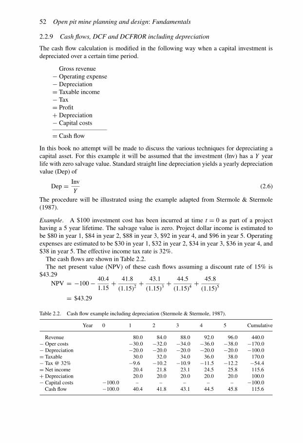
52 Open pit mine planning and design: Fundamentals
2.2.9 Cash flows, DCF and DCFROR including depreciation
The cash flow calculation is modified in the following way when a capital investment isdepreciated over a certain time period.
Gross revenue− Operating expense− Depreciation= Taxable income− Tax= Profit+ Depreciation− Capital costs
= Cash flow
In this book no attempt will be made to discuss the various techniques for depreciating acapital asset. For this example it will be assumed that the investment (Inv) has a Y yearlife with zero salvage value. Standard straight line depreciation yields a yearly depreciationvalue (Dep) of
Dep = Inv
Y(2.6)
The procedure will be illustrated using the example adapted from Stermole & Stermole(1987).
Example. A $100 investment cost has been incurred at time t = 0 as part of a projecthaving a 5 year lifetime. The salvage value is zero. Project dollar income is estimated tobe $80 in year 1, $84 in year 2, $88 in year 3, $92 in year 4, and $96 in year 5. Operatingexpenses are estimated to be $30 in year 1, $32 in year 2, $34 in year 3, $36 in year 4, and$38 in year 5. The effective income tax rate is 32%.The cash flows are shown in Table 2.2.The net present value (NPV) of these cash flows assuming a discount rate of 15% is
$43.29NPV = −100 − 40.4
1.15+ 41.8
(1.15)2+ 43.1
(1.15)3+ 44.5
(1.15)4+ 45.8
(1.15)5
= $43.29
Table 2.2. Cash flow example including depreciation (Stermole & Stermole, 1987).
Year 0 1 2 3 4 5 Cumulative
Revenue 80.0 84.0 88.0 92.0 96.0 440.0− Oper costs −30.0 −32.0 −34.0 −36.0 −38.0 −170.0− Depreciation −20.0 −20.0 −20.0 −20.0 −20.0 −100.0= Taxable 30.0 32.0 34.0 36.0 38.0 170.0− Tax @ 32% −9.6 −10.2 −10.9 −11.5 −12.2 −54.4= Net income 20.4 21.8 23.1 24.5 25.8 115.6+ Depreciation 20.0 20.0 20.0 20.0 20.0 100.0− Capital costs −100.0 – – – – – −100.0
Cash flow −100.0 40.4 41.8 43.1 44.5 45.8 115.6

Mining revenues and costs 53
The DCFROR is the discount rate which makes the net present value equal to zero. In thiscase
NPV = −100 − 40.4
1 + i+ 41.8
(1 + i)2+ 43.1
(1 + i)3+ 44.5
(1 + i)4+ 45.8
(1 + i)5= 0
The value of i is about
i ∼= 0.315
2.2.10 Depletion
In the U.S. special tax consideration is given to the owner of a mineral deposit which isextracted (depleted) over the production life. One might consider the value of the deposit to‘depreciate’ much the same way as any other capital investment. Instead of ‘depreciation’,the process is called ‘depletion’. The two methods for computing depletion are:(1) cost depletion,(2) percentage depletion.Each year both methods are applied and that which yields the greatest tax deduction
is chosen. The method chosen can vary from year to year. For most mining operations,percentage depletion normally results in the greatest deduction.To apply the cost depletion method, one must first establish the cost depletion basis. The
initial cost basis would normally include:– the cost of acquiring the property including abstract and attorney fees.– exploration costs, geological and geophysical survey costs.
To illustrate the principle, assume that this is $10. Assume also that there are 100 tons ofreserves and the yearly production is 10 tons. The $10 cost must then be written off over the100 total tons. For the calculation of cost depletion the cost basis at the end of any year (notadjusted by the current years depletion) is divided by the estimated remaining ore reserveunits plus the amount of ore removed during the year. This gives the unit depletion. In thissimple case, for year 1
Unit depletion = $10
100= $0.10
The unit depletion is then multiplied by the amount of ore extracted during the year to arriveat the depletion deduction,
Depletion deduction = 10 tons × $0.10 = $1
The new depletion cost basis is the original cost basis minus the depletion to date. Thus forthe year 2 calculation:
Depletion cost basis = $10 − $1 = $9
Remaining reserves = 90 tons
The year 2 unit depletion and depletion deduction are:
Unit depletion = $9
90= $0.10
Depletion deduction = 10 × $0.10 = $1

54 Open pit mine planning and design: Fundamentals
Table 2.3. Percentage depletion rates for the more common minerals. A complete list of minerals and theirpercentage depletion rates are given in section 613(b) of the Internal Revenue Code.
Deposits Rate
Sulphur, uranium, and, if from deposits in the United States, asbestos, lead ore,zinc ore, nickel ore, and mica 22 %Gold, silver, copper, iron ore, and certain oil shale, if from depositsin the United States 15 %Borax, granite, limestone, marble, mollusk shells, potash, slate, soapstone,and carbon dioxide produced from a well 14 %Coal, lignite, and sodium chloride 10 %Clay and shale used or sold for use in making sewer pipe or bricks or usedor sold for use as sintered or burned lightweight aggregates 7½ %Clay used or sold for use in making drainage and roofing tile, flower pots, and kindredproducts, and gravel, sand, and stone (other than stone used or sold for use by amine owner or operator as dimension or ornamental stone) 5 %
IRS 2011. Depletion.Ref: www.irs.gov/publications/p535/ch09.html
Once the initial cost of the property has been recovered, the cost depletion basis is zero.Obviously, the cost depletion deduction will remain zero for all succeeding years.The percent depletion deduction calculation is a three step process. In the first step, the
percent deduction is found by multiplying a specified percentage times the gross miningincome (after royalties have been subtracted) resulting from the sale of theminerals extractedfrom the property during the tax year. According to Stermole & Stermole (1987):
‘Mining’ includes, in addition to the extraction of minerals from the ground, treatmentprocesses considered as mining applied by the mine owner or operator to the mineralsor the ore, and transportation that is not over 50 miles from the point of extraction tothe plant or mill in which allowable treatment processes are applied. Treatment processesconsidered as mining depend upon the ore or mineral mined, and generally include thoseprocesses necessary to bring the mineral or ore to the stage at which it first becomescommercially marketable; this usually means to a shipping grade and form. However, incertain cases, additional processes are specified in the Internal Revenue Service regulations,and are considered as mining. Net smelter return or its equivalent is the gross income onwhich mining percentage depletion commonly is based. Royalty owners get percentagedepletion on royalty income so companies get percentage depletion on gross income afterroyalties.
As shown in Table 2.3, the percentage which is applied varies depending on the type ofmineral being mined.In step 2, the taxable income (including all deductions except depletion and carry forward
loss) is calculated for the year in question. Finally in step 3, the allowable percentagedepletion deduction is selected as the lesser of the percent depletion (found in step 1) and50% of the taxable income (found in step 2).With both the allowable cost depletion and percentage depletion deductions now calcu-
lated, they are compared. The larger of the two is the ‘allowed depletion deduction’. Theoverall process is summarized in Figure 2.1.

Mining revenues and costs 55
Figure 2.1. Flow sheet for determining the depletion deduction (Stermole & Stermole, 1987).
2.2.11 Cash flows, including depletion
As indicated the depletion allowance works exactly the same way in a cash flow calculationas depreciation. With depletion the cash flow becomes:
Gross revenue− Operating expense− Depreciation− Depletion− Taxable income− Tax= Profit+ Depreciation+ Depletion− Capital costs
= Cash flow
The following simplified example adapted from Stermole & Stermole (1987) illustrates theinclusion of depletion in a cash flow calculation.
Example. Amining operation has an annual sales revenue of $1,500,000 from a silver ore.Operating costs are $700,000, the allowable depreciation is $100,000 and the applicable taxrate is 32%. The cost depletion basis is zero. The cash flow is:
(1) Preliminary. Calculation without depletion.
Gross revenue $1,500,000− Operating expense −700,000− Depreciation −100,000
= Taxable income before depletion $700,000
(2) Depletion calculation. Since the depletion basis is zero, percentage depletion is theonly one to be considered. One must then choose the smaller of:(a) 50% of the taxable income before depletion and carry-forward-losses(b) 15% of the gross revenue

56 Open pit mine planning and design: Fundamentals
In this case the values are:(a) 0.50 × $700,000 = $350,000(b) 0.15 × $1,500,000 = $225,000
Hence the depletion allowance is $225,000.
(3) Cash flow calculation.
Gross revenue $1,500,000− Operating expense −700,000− Depreciation −100,000− Depletion −225,000
= Taxable income $475,000− Tax @ 32% −152,000
= Profit $323,000+ Depreciation +100,000+ Depletion +225,000
= Cash flow $648,000
The cash flow calculation process is expressed in words (Laing, 1976) in Table 2.4.Laing (1976) has summarized (see Table 2.5) the factors which should be considered
when making a cash flow analysis of a mining property.The distinction between the ‘exploration’ and ‘development’ phases of a project is often
blurred in actual practice. However from a tax viewpoint a sharp distinction is often made.The distinction made by the U.S. Internal Revenue Service (1988a) is paraphrased below.
1. The exploration stage involves those activities aimed at ascertaining the existence, loca-tion, extent or quality of any deposit of ore or other mineral (other than oil or gas).Exploration expenditures paid for or incurred before the beginning of the developmentstage of the mine or other natural deposit may for tax purposes be deducted from currentincome. If, however, a producing mine results, these expenditures must be ‘recaptured’ andcapitalized. These are later recovered through either depreciation or cost depletion.
2. The development stage of the mine or other natural deposit will be deemed to begin atthe time when, in consideration of all the facts and circumstances, deposits of ore or othermineral are shown to exist in sufficient quantity and quality to reasonably justify exploitation.Expenditures on amine after the development stage has been reached are treated as operatingexpenses.
For further information concerning the economic models the interested reader is referred toStermole & Stermole (2012).
2.3 ESTIMATING REVENUES
2.3.1 Current mineral prices
Current mineral prices may be found in a number of different publications. Metals Week,Mining Magazine, Metal Bulletin and Industrial Minerals are four examples. Spot prices

Mining revenues and costs 57
Table 2.4. Components of an annual cash flow analysis for a miningproperty (Laing, 1976).
Calculation Component
Revenueless Operating costs
equals Net income before depreciation and depletion
less Depreciation and amortization allowance
equals Net income after depreciation and amortization
less Depletion allowance
equals Net taxable income
less State income tax
equals Net federal taxable income
less Federal income tax
equals Net profit after taxes
add Depreciation and amortization allowances
add Depletion allowance
equals Operating cash flow
less Captial expenditures
less Working capital
equals Net annual cash flow
Table 2.5. Factors for consideration in a cash flow analysis of a mining property (Laing,1976).
Preproduction period
Exploration expenses Land and mineral rightsWater rights Environmental costsMine and plant capital requirements Development costsSunk costs Financial structureWorking capital Administration
Production period
Price Capital investment-replacement and expansionsProcessing costs RoyaltyRecovery Mining costPost concentrate cost Development costReserves and percent removable Exploration costGrade General and administrationInvestment tax credit InsuranceState taxes Production rate in tons per yearFederal taxes Financial year production beginsDepletion rate Percent production not sent to processing plantDepreciation schedule Operating days per year
Post production period
Salvage value Contractual and reclamation expenditures

58 Open pit mine planning and design: Fundamentals
for the major metals are listed in the business sections of many daily newspapers togetherwith futures prices. Tables 2.6 through 2.8 contain 1992–93 prices for certain:
– metals– nonmetallic minerals– miscellaneous metals– ferro alloys– ores and concentrates.
In reviewing the tables it is seen that there is considerable variation in how the prices arequoted. In general, the prices depend upon:
– quality– quantity– source– form– packaging.
The units in which the prices are expressed also vary. Some examples in this regard arepresented below.
1. For many minerals, the ‘ton’ is unit of sale. There are three different ‘tons’ whichmight be used. They are:
1 short ton (st) = 2000 lbs = 0.9072 metric tons
1 long ton (lt) = 2240 lbs = 1.01605 metric tons
1 metric ton (mt or tonne) = 2204.61 lbs
= 1000 kilograms
= 0.9842 long tons
= 1.1023 short tons
Iron ore, sulfur, and manganese ore are three materials normally sold by the long ton. Theprices for iron ore and manganese ore are expressed in X dollars (or cents) per long ton unit(ltu). A ‘unit’ refers to the unit in which the quality of the mineral is expressed. For iron orethe quality is expressed in Y% Fe. Therefore one unit means 1%.If 1 long ton (2240 lbs) of iron ore contained 1% iron (22.40 lbs), then it would contain 1
long ton unit (1 ltu) of iron. If the long ton assayed at 65% iron then it would contain 65 ltu.If the quoted price for pellets is 70� c/ltu, then the price of 1 long ton of pellets running 65%iron would be:
price/long ton = 65 × 70 � c = 4550 � c/lt= $45.50/lt
Metric ton units (mtu) and short ton units (stu) are dealt with in the same way.The reason for using the ‘unit’ approach is to take into account varying qualities.2. For most metals, the unit of weight is the pound (lb) or kilogram (kg).3. Gold, silver, platinum, palladium, and rhodium are sold by the troy ounce.

Mining revenues and costs 59
Table 2.6. Metal prices (E/MJ, 1993).

60 Open pit mine planning and design: Fundamentals
Table 2.7. Prices for some common non-metallic minerals (Industrial Minerals, December 1992).Copyright 1992. Industrial Minerals, reproduced with permission.
To accord with trade practices, certain prices are quoted in US$ (sterling now floating at around $1.50–1.70= £1). All quotationsare © Metal Bulletin plc 1992.

Mining revenues and costs 61
Table 2.8. Prices* for some common non-ferrous ores (Metal Bulletin, 1993). Copyright 1993 MetalBulletin; reproduced with permission.
*Prices expressed C.I.F. Europe unless otherwise indicated.

62 Open pit mine planning and design: Fundamentals
The relationship between the troy ounce and some other units of weight are given below.
Troy weight (tr)
1 troz = 31.1035 grams
= 480 grains
= 20 pennyweights(dwt)
= 1.09714 oz avoird
U.S. Standard (avoirdupois)
1 ozavoird = 28.3495 grams
= 437.5 grains
1 lb = 16 oz
= 14.5833 tr oz
= 453.59 grams
4. Mercury (quicksilver) is sold by the flask. A ‘flask’ is an iron container which holds76 lbs of mercury.5. Molybdenum is sometimes quoted in the oxide (roasted) form (MoO3) or as the sulfide
(MoS2). The price given is per pound of Mo contained. For the oxide form this is about 67%and for the sulfide 60%.6. The forms in which minerals are sold include bulk, bags, cathodes, ingots, rods,
slabs, etc.7. The purity of the mineral products often have a substantial effect on price (see for
example Feldspar).8. The fiber length and quality is extremely important to asbestos.
The point of sale also has a considerable effect on the price. Two abbreviations are oftenused in this regard.The abbreviation ‘F.O.B.’ stands for ‘free-on-board’. Thus the designation ‘F.O.B. mine’
means that the product would be loaded into a transport vessel (for example, rail cars) butthe buyer must pay all transport charges from the mine to the final destination.The abbreviation ‘C.I.F.’means that cost, insurance and freight are included in the price.Table 2.9 illustrates the difference in price depending on delivery point. For USX Corp.
pellets, the price of 37.344� c/ltu is at the mine (Mountain Iron, Minnesota). The Cleveland-Cliffs price of 59.4� c/ltu (also for Minnesota taconite pellets) is at the hold of the ship atthe upper lake port. Hence a rail charge has now been imposed. For the Oglebay NortonCo. (Minnesota) pellets, the price of 72.45� c/ltu is at the lower lake port. Thus it includesrail transport from the mine to the upper lake port plus ship transport to the lower lake port.Table 2.10 provides freight rates for iron ore and pellets. Lake freight rates are given inTable 2.11.
Many mineral products are sold through long term contracts arranged between supplierand customer. The prices will reflect this shared risk taking. There will often be significantdifferences between the short term (spot) and long term prices.Recent prices for metals and industrial minerals are provided in Tables 2.12 and 2.13.
Table 2.14 presents the prices for iron ore from various suppliers in 2005.

Mining revenues and costs 63
Table 2.9. Iron ore prices (Skillings Mining Review, 1993a).
Lake Superior iron ore prices(Per gross ton, 51.50% iron natural, at rail of vessel lower lake port)Mesabi non-Bessemer . . . . . . . . . . . . . . . . . . . . . . . . . . . . . . . . . . . . . . . . . . . . . . . . . . . . . . . . . . . . . . . . $30.03-31.53
Cleveland-Cliffs Inc iron ore pellet prices(Per iron natural unit, at rail of vessel lower lake port)Cleveland-Cliffs Inc . . . . . . . . . . . . . . . . . . . . . . . . . . . . . . . . . . . . . . . . . . . . . . . . . . . . . . . . . . . . . . . . . . . . . . . 72.45� cPer gross ton unit at hold of vessel upper lake port . . . . . . . . . . . . . . . . . . . . . . . . . . . . . . . . . . . . . . . . . . . . 53.40� cWabush pellets per gross ton unit F.O.B. Pointe Noire . . . . . . . . . . . . . . . . . . . . . . . . . . . . . . . . . . . . . . . . . 63.50� cCyprus Northshore Mining Corp. pellet price(Per gross ton iron unit natural F.O.B. Silver Bay)Cyprus Northshore pellets . . . . . . . . . . . . . . . . . . . . . . . . . . . . . . . . . . . . . . . . . . . . . . . . . . . . . . . . . . . . . . . . . . 48.76� cIOC Ore Sales Co. pellet price(Per natural gross ton unit delivered rail of vessel lower lake port)Carol pellets . . . . . . . . . . . . . . . . . . . . . . . . . . . . . . . . . . . . . . . . . . . . . . . . . . . . . . . . . . . . . . . . . . . . . . . . . . . . . . 74.65� cInland Steel Mining Co. pellet pricePer gross ton natural iron unit at hold vessel upper lake port . . . . . . . . . . . . . . . . . . . . . . . . . . . . . . . . . . . 46.84� cOglebay Norton Co. pellet prices(Per natural gross ton unit, at rail of vessel lower lake port)Standard grade . . . . . . . . . . . . . . . . . . . . . . . . . . . . . . . . . . . . . . . . . . . . . . . . . . . . . . . . . . . . . . . . . . . . . . . . . . . . 72.45� cEveleth special . . . . . . . . . . . . . . . . . . . . . . . . . . . . . . . . . . . . . . . . . . . . . . . . . . . . . . . . . . . . . . . . . . . . . . . . . . . . 74.00� cU.S. Steel pellet pricePer dry gross ton iron unit at Mtn. Iron . . . . . . . . . . . . . . . . . . . . . . . . . . . . . . . . . . . . . . . . . . . . . . . . . . . . . 37.344� c
Table 2.10. Rail tariff rates on iron ore and pellets (Skillings Mining Review, 1993b).
Rail freight rates ($/gross ton) from mines to Upper Lake PortMarquette Range to Presque Isle
Pellets . . . . . . . . . . . . . . . . . . . . . . . . . . . . . . . . . . . . . . . . . . . . . . . . . . . . . . . . . . . . . . . . . . . . . . . . . . . . . . . . . . . $2.50Natural ore . . . . . . . . . . . . . . . . . . . . . . . . . . . . . . . . . . . . . . . . . . . . . . . . . . . . . . . . . . . . . . . . . . . . . . . . . . . . . . . . 2.56
Pellets from Marquette Range to Escanaba delivered into vessel . . . . . . . . . . . . . . . . . . . . . . . . . . . . . . . . . . 3.39Mesabi Range plants on BN to:Allouez delivered direct into vessel . . . . . . . . . . . . . . . . . . . . . . . . . . . . . . . . . . . . . . . . . . . . . . . . . . . . . . . . . . 6.16When consigned to storage subject to storage charges . . . . . . . . . . . . . . . . . . . . . . . . . . . . . . . . . . . . . . . . . 6.53
Winter ground storage charges on pellets:At Allouez per gross ton per month . . . . . . . . . . . . . . . . . . . . . . . . . . . . . . . . . . . . . . . . . . . . . . . . . . . . . . . . . 16.0� cAt Escanaba: storage per gross ton per month . . . . . . . . . . . . . . . . . . . . . . . . . . . . . . . . . . . . . . . . . . . . . . . . 2.4� c
handling to storage . . . . . . . . . . . . . . . . . . . . . . . . . . . . . . . . . . . . . . . . . . . . . . . . . . . . . . . . . . . . . . . . . . . . . 21.8� chandling from storage . . . . . . . . . . . . . . . . . . . . . . . . . . . . . . . . . . . . . . . . . . . . . . . . . . . . . . . . . . . . . . . . . . 21.8� c
Dock charges on iron ore per gross tonCar to vessel at Duluth and Two Harbors . . . . . . . . . . . . . . . . . . . . . . . . . . . . . . . . . . . . . . . . . . . . . . . . . . . . . . $1.05
All-rail freight rates to consuming districtsMesabi Range to:
Chicago district . . . . . . . . . . . . . . . . . . . . . . . . . . . . . . . . . . . . . . . . . . . . . . . . . . . . . . . . . . . . . . . . . . . . . . . . . . 20.42Geneva, Utah . . . . . . . . . . . . . . . . . . . . . . . . . . . . . . . . . . . . . . . . . . . . . . . . . . . . . . . . . . . . . . . . . . . . . . . . . . . *46.97Granite City and East St. Louis, Ill. . . . . . . . . . . . . . . . . . . . . . . . . . . . . . . . . . . . . . . . . . . . . . . . . . . . . . . . . . 19.69Valley district . . . . . . . . . . . . . . . . . . . . . . . . . . . . . . . . . . . . . . . . . . . . . . . . . . . . . . . . . . . . . . . . . . . . . . . . . . . . 40.17
Marquette Range to Detroit . . . . . . . . . . . . . . . . . . . . . . . . . . . . . . . . . . . . . . . . . . . . . . . . . . . . . . . . . . . . . . . . . . 28.60Marquette & Menominee Ranges to:
Chicago district . . . . . . . . . . . . . . . . . . . . . . . . . . . . . . . . . . . . . . . . . . . . . . . . . . . . . . . . . . . . . . . . . . . . . . . . **24.09Granite City and East St. Louis, Ill. . . . . . . . . . . . . . . . . . . . . . . . . . . . . . . . . . . . . . . . . . . . . . . . . . . . . . . . . . 23.18
*Conditional on tender of not less than 4800 GT nor more than 5200 GT.**Multiple car rate.

64 Open pit mine planning and design: Fundamentals
Table 2.11. Lake freight tariff rates on iron ore, pellets and limestone (Skillings Mining Review, 1993c).
Lake freight rates from Upper Lake ports to Lower Lake ports
Iron ore ($/gross ton) Self unloading vesselsHead of Lakes to Lower Lakes . . . . . . . . . . . . . . . . . . . . . . . . . . . . . . . . . . . . . . . . . . . . . . . . . . . . . . . . . . . . . . . $6.50Marquette to Lower Lakes . . . . . . . . . . . . . . . . . . . . . . . . . . . . . . . . . . . . . . . . . . . . . . . . . . . . . . . . . . . . . . . . . . . . 5.40Escanaba to Lake Erie . . . . . . . . . . . . . . . . . . . . . . . . . . . . . . . . . . . . . . . . . . . . . . . . . . . . . . . . . . . . . . . . . . . . . . . . 4.88Escanaba to Lake Michigan . . . . . . . . . . . . . . . . . . . . . . . . . . . . . . . . . . . . . . . . . . . . . . . . . . . . . . . . . . . . . . . . . . . 3.90
Limestone ($/gross ton)Calcite, Drummond, Cedarville and Stoneport to
Lower Lake Michigan . . . . . . . . . . . . . . . . . . . . . . . . . . . . . . . . . . . . . . . . . . . . . . . . . . . . . . . . . . . . . . . . . . . . . . 3.98Lake Erie ports . . . . . . . . . . . . . . . . . . . . . . . . . . . . . . . . . . . . . . . . . . . . . . . . . . . . . . . . . . . . . . . . . . . . . . . . . . . . 4.10
Note: The above cargo rates apply after April 15 and before December 15, 1993. Winter formulasapply during other periods. Rates are further subject to surcharges, if warranted.
Dock, handling and storage charges ($/gross ton) on iron ore at Lower Lake ports RCCR X-088C
Ex self-unloading vessels at Cleveland, OhioDockage . . . . . . . . . . . . . . . . . . . . . . . . . . . . . . . . . . . . . . . . . . . . . . . . . . . . . . . . . . . . . . . . . . . . . . . . . . . . . . . . . . . $0.26
From dock receiving area into cars, via storage . . . . . . . . . . . . . . . . . . . . . . . . . . . . . . . . . . . . . . . . . . . . . . . 1.60From dock receiving area to cars . . . . . . . . . . . . . . . . . . . . . . . . . . . . . . . . . . . . . . . . . . . . . . . . . . . . . . . . . . . . 1.05
Rail of vessel receiving area to cars . . . . . . . . . . . . . . . . . . . . . . . . . . . . . . . . . . . . . . . . . . . . . . . . . . . . . . . . . . . . 1.16
At Conneaut, Ohio BLEDockage of self-unloading vessel . . . . . . . . . . . . . . . . . . . . . . . . . . . . . . . . . . . . . . . . . . . . . . . . . . . . . . . . . . . . . $0.15
From receiving bin to storage . . . . . . . . . . . . . . . . . . . . . . . . . . . . . . . . . . . . . . . . . . . . . . . . . . . . . . . . . . . . . . . 0.53From storage to railcars . . . . . . . . . . . . . . . . . . . . . . . . . . . . . . . . . . . . . . . . . . . . . . . . . . . . . . . . . . . . . . . . . . . . 0.68
Ex bulk vessels at Cleveland C&PFrom hold to rail of vessel . . . . . . . . . . . . . . . . . . . . . . . . . . . . . . . . . . . . . . . . . . . . . . . . . . . . . . . . . . . . . . . . . . . $1.03From rail of vessel into car . . . . . . . . . . . . . . . . . . . . . . . . . . . . . . . . . . . . . . . . . . . . . . . . . . . . . . . . . . . . . . . . . . . . 1.26From rail of vessel via storage into car . . . . . . . . . . . . . . . . . . . . . . . . . . . . . . . . . . . . . . . . . . . . . . . . . . . . . . . . . 2.25
2.3.2 Historical price data
Mineral prices as monitored over a time span of many years exhibit a general upwardtrend. However, this is not a steady increase with time but rather is characterized by cyclicfluctuations. Table 2.15 shows the average yearly prices for 10 common metals from 1900through 2011 (USGS, 2012a). The monthly and average prices for 11 common metals forthe period January 1997 through July 2012 are given inTable 2.16 (Metal Bulletin, 2012). Toprovide an indication of the price unpredictability, consider the case of copper. In 1900 forexample the copper price was about 16.2� c/lb (Table 2.15). In 2000, 100 years later, the pricehad risen to 82� c/lb. The average rate of price increase per year over this period using the endpoint values is 1.6 percent. The price dropped to a lowof 5.8� c/lb (1932) and reached a high of131� c/lb (1989) over this period. Using the average price increase over the period of 1900 to2000, the predicted price in 1950 should have been 36.4� c/lb. The actual value was 21.2� c/lb.A mining venture may span a few years or several decades. In some cases mines have
produced over several centuries. Normally a considerable capital investment is required tobring a mine into production. This investment is recovered from the revenues generated overthe life of the mine. The revenues obviously are strongly dependent upon mineral price. Ifthe actual price over themine life period is less than that projected, serious revenue shortfallswould be experienced. Capital recovery would be jeopardized to say nothing of profits.Price trends, for metals in particular, are typically cyclic. Using the metal price data
from Table 2.15, Figures 2.2 through 2.6 show the prices for 10 metals over the period1950 through 2011. The period and amplitude of the cycles varies considerably. For nickel

Mining revenues and costs 65
Table 2.12. Recentweeklymetal prices (PlattsMetalsWeek, 2012,April 16). Copyright 2012 PlattsMetalsWeek; reproduced with permission.
Major Metals
Aluminumcts/lb
MW US Market 101.750/102.750US Six-Months P1020 9.500US 6063 Billet Upcharge 10.500/12.500US UBCs 78.500/80.000Painted Siding 79.000/80.000US 6063 press scrap 4.500/5.500
Eur/mtAlloy 226 deliveredEuropean works
1700.000/ 1750.000
$/mtADC12 FOB China 2310.000/2320.000
Yuan/mtADC12 ex-works China 17400.000/17600.000
Caustic Soda$/mt
FOB NEAsia 422.000/424.000CFR SEAsia 476.000/478.000
Coppercts/lb
MW No.1 Burnt Scrap Disc 19.000MW No.1 Bare Bright Disc 3.000MW No.2 Scrap Disc 39.000NY Dealer Premiumcathodes
5.500/6.500
US Producer cathodes 371.650/379.090$/mt
Grade A Cathode CIFR’dam
8253.000/8260.000
Grade A Premium CIFR’dam
75.000/80.000
Grade A CIFLivorno/Salerno
8228.000/8240.000
Grade A Prem CIFLivorno/Salerno
50.000/60.000
Russian Standard CIFR’dam
8178.000/8210.000
Russian Standard Prem CIFR’dam
0.000/30.000
Leadcts/lb
North American Market 98.830/101.643$/mt
European dealer 2072.000/2088.000European 99.985%Prem IW(R’dam)
20.000/35.000
In-Warehouse S’pore Prem 50.000/80.000
Nickel$/lb
NY Dealer/Cathode 8.403/8.555
NY Dealer/Melting 8.403/8.555NY Dealer/Plating 8.603/8.755
cts/lbNY Dealer/CathodePremium
30.000
NY Dealer/MeltingPremium
30.000
NY Dealer/PlatingPremium
50.000
$/mtPlating Grade IW R’dam 18324.000/18384.000Plating Grade PremIW R’dam
200.000/250.000
Russia Full-Plate 18184.000/18214.000Russia Full-Plate PremIW R’dam
60.000/80.000
Briquette PremiumIW R’dam
200.000/250.000
In-Warehouse S’porePrem
150.000/160.000
Tin$/mt
Europe 99.85% IWR’dam
22956.000/23094.000
Europe 99.85% PremIW R’dam
300.000/400.000
Europe 99.90% IWR’dam
23156.000/23244.000
Europe 99.90% PremIW R’dam
500.000/550.000
Zinccts/lb
US Dealer SHG 98.921MW SHG Premium 7.250MW SHG Galv. Prem. 7.000MW SHGAlloyer #3Prem.
17.000
$/mtEurope physical SHGIW R’dam
2109.000/2129.000
Europe physical SHGPrem IW R’dam
105.000/125.000
In-Warehouse S’porePrem
70.000/95.000
Precious Metals
All PGM figures in $/tr ozIridiumMW NY Dealer 1050.000/1085.000OsmiumMW NY Dealer 350.000/400.000PalladiumMW NY Dealer 630.000/655.000
(Continued)

66 Open pit mine planning and design: Fundamentals
Table 2.12. (Continued).
PlatinumMW NY Dealer 1580.000/1630.000RhodiumMW NY Dealer 1300.000/1375.000RutheniumMW NY Dealer 95.000/115.000
Minor Metals
Antimonycts/lb
MW NY Dealer 590.000/620.000$/mt
99.65% FOB China 13000.000/13200.000
Arseniccts/lb
MW Dealer 60.000/70.000
Bismuth$/lb
MW NY Dealer 10.400/11.250
Cadmium$/lb
MW NY Dealer 0.950/1.150Free Market HG 1.000/1.200
Indium$/kg
Producer: US Prod IndiumCorp
785.000
MW NY Dealer 540.000/570.00099.99% CIF Japan 560.000/570.000
Mercury$/fl
Free Market International 1750.000/1950.000U.S. Domestic 1750.000/1950.000
Rhenium$/kg
MW NY Dealer 4200.000/4800.000
Selenium$/lb
MW NY Dealer 61.000/66.000
Light Metals
Magnesiumcts/lb
US Die Cast Alloy:Transaction
200.000/220.000
MW US Spot Western 215.000/230.000MW US Dealer Import 200.000/210.000
$/mtEurope Free Market 3100.000/3200.000Die Cast Alloy FOB China 3280.000/3340.00099.8% FOB China 3000.000/3050.000
Siliconcts/lb
553 Grade DeliveredUS Midwest
127.000/130.000
$/mt553 Grade, FOB China 2250.000/2300.000553 Grade, CIF Japan 2280.000/2340.000
Eur/mt553 Grade,In-warehouse EU
1950.000/2050.000
Titanium$/lb
MW US 70% Ferrotitanium 3.600/3.650$/kg
Eur. 70% Ferrotitanium 8.000/8.200$/lb
MW US Turning 0.5% 2.150/2.300Eur. Turning .5% 2.300/2.400
Ferroalloys
Cobalt
MW 99.8% US SpotCathode
$/lb
99.8% European 15.000/15.75099.3% Russian 15.000/15.60099.6% Zambian 14.800/15.200
14.700/15.000Ferrochrome
cts/lbCharge Chrome 48–52%in-warehouse US
118.000/122.000
65% High Carbonin-warehouse US
118.000/122.000
Low Carbon 0.05%in-warehouse US
235.000/240.000
Low Carbon 0.10%in-warehouse US
218.000/222.000
Low Carbon 0.15%in-warehouse US
205.000/210.000
Charge Chrome 52%DDP NWE
103.000/110.000
65%–68% High-CarbonDDP NWE
120.000/123.000
Low Carbon 0.10% DDPNWE
215.000/220.000
High Carbon 60% FOBChina
100.000/104.000
50–55% Regular CIF Japan 123.00060–65% Spot CIF Japan 109.000/111.000
Ferromanganese$/gt
High Carbon 76%in-warehouse US
1275.000/1350.000
(Continued)

Mining revenues and costs 67
Table 2.12. (Continued).
cts/lbMedium Carbon 85% Mnin-warehouse US
95.000/96.000
$/mtHigh Carbon 75% FOB China 1200.000/1210.000
Ferromolybdenum$/lb
MW US FeMo 16.100/16.400$/kg
MW Europe FeMo 34.200/34.600FOB China FeMo 34.400/34.500Spot CIF Japan 34.900/35.000
Ferrosiliconcts/lb
75% Si in-warehouse US 94.000/96.000$/mt
Chinese CIF Japan 1420.000/1435.000$/mt
75% FOB China 1420.000/1430.000Eur/mt
75% Std DDP NWE 1230.000/1290.000
Ferrovanadium$/lb
Free Market V205 5.500/6.000US Ferrovanadium 14.250/14.750
$/kgEurope Ferrovanadium 25.700/26.000
Manganese$/mt
Electrolytic 99.7% FOB China 3000.000/3050.000
Molybdenum$/lb
MW Dealer Oxide 14.150/14.300Oxide Trans 14.150/14.300
Silicomanganesects/lb
65% Mn in-warehouse US 73.000/75.000$/mt
65% FOB China 1480.000/1500.000Chinese CIF Japan 1400.000/1500.000
Eur/mt65:16 DDP NWE 1020.000/1050.000
Stainless Scrap$/gt
NA FREE MKT 18-8 1792.000/1837.000
Tantalum$/lb
Spot Tantalite Ore 37.000/42.000
Tungsten$/stu
MW US Spot Ore 320.000/330.000APT-US 395.000/420.000
$/mtuAPT FOB China 400.000/410.000
$/kgMW Ferrotungsten 54.000/55.000Ferrotungsten FOB 53.000/56.500
consider the period from 1983 through 1998. In 1983, the price began at $2.12/lb, droppedto $1.76/lb in 1986, and rose to a high of $6.25/lb in 1988. It then dropped to $2.40/lbin 1993 before increasing once again to $3.73/lb in 1995 before landing in 1998 at aboutthe same price it started at in 1983. Starting in 2002, the nickel price again began risingdramatically, reaching $16.87/lb in 2007, falling to $6.62/lb in 2009, and then stabilizingsomewhat to around 10.00$/lb for the years 2010 and 2011.In 1975, silver was around $4.50/tr oz. It shot up to nearly $40.00/tr oz (January 1980)
due to the buying of the Hunt brothers from Texas. By the end of 1991, the price haddropped back to about $4.50/tr oz. Recently the price of silver has again been risingdramatically, reaching $34.50/tr oz in 2011.The price performance of iron ore fines over the period 1900–2011 is presented in Table
2.17 (USGS, 2012b). The monthly spot price for China import iron ore fines over the periodJanuary 2000 through July 2012 is presented in Table 2.18 (IMF, 2012) and in Figure 2.7.In the past, the iron ore price each year was set in January and was constant throughout theyear. Starting in November 2008, the price began varying monthly reflecting that major ironore production began moving from long term annual contracts to quarterly, monthly, andthen pure spot market prices.

68 Open pit mine planning and design: Fundamentals
Table 2.13. Prices for some common industrial minerals (IndustrialMinerals, 2012. Monthly Prices -June)(All prices are in US$ and quoted per tonne unless indicated.).
AluminaCalcined 98.5–99.5%Al2O3 bulkFOB US refinery
$675–725
Calcined, ground 98.5–99.5%Al2O3,bulk FOB US refinery
$750–850
Calcined, medium-soda Al2O3, bulkFOB refinery
$800–850
Alumina, fusedBrown 95% min. Al2O3, FEPAF8-220 Grit, FOB China
$800–840
Brown 95.5%Al2O3, refractorylump & sized, FOB China
$660–730
White, 25 kg bags, CIF Europe a850–890Brown 94%Al2O3, FEPA 8-220mesh refractory (mm) Chinese
$750–850
Andalusite57–58%Al2O3, 2,000 tonne bulk,FCA Mine-RSA
a235–280
55–59%Al2O3, FOB European port a350–425
Antimony TrioxideTypically 99.5% SbO3, 5 tonne lots,CIF Antwerp/Rotterdam
$11,100–11,200
Typically 99.5% SbO3, 20 tonnelots FOB China
$11,100–11,200
Typically 99.5% SbO3,ex-works USA
$11,100–11,200
Ingot, 99.65% min, CIF Rotterdam $13,500–13,700Ingot, 99.65% min, FOB China $13,500–13,600
BaddeleyiteContract price, Refractory/abrasivegrade, CIF main European port
$2500–3100
Contract price, Ceramic grade (98%ZrO2 +HfO2), CIF mainEuropean port
$3000–3300
Contract price, Ceramic pigmentgrade, CIF main European port
$3200–3500
BarytesDrilling gradeUnground lumpOCMA/API bulk, SG 4.20
FOB Chennai $146–150FOB Morocco $147–150FOB China $155–158
C&F North Sea (Moroccan) $160–167API, CIF Gulf Coast,
Chinese $166–182Indian $157–171
GroundOCMA bulk, del. Aberdeen £95–105OCMA bulk, del. GtYarmouth £110–120OCMA/API, big bags (1.5t), FOBS. Turkey
$150–155
SG 4.22, bagged, FOB Morocco $135–147
Paint gradeGround white 96–98% BaSO4,350 mesh, 1–5 lots, del. UK
£195–220
Chinese lump, CIF Gulf Coast $250–290Ground, white, 96–98% BaSO4,325–350 mesh, 1–5 lots,ex-works USA. $/s. ton
$315–400
Chemical gradeChinese, CIF Gulf Coast $170–182
BauxiteRefractory gradeChinese Al2O3/Fe2O3/BD,lumps 0–25mm Shanxi,FOB XingangRound kiln 87/2.0/3.2 $395–430Round kiln 86/2.0/3.15–3.20 $360–440Round kiln 85/2.0/3.15 $370–410Rotary kiln 86/1.8/3.15 $365–435Rotary kiln 85/1.8/3.15 $350–450
Guizhou, FOB Zhanjiang/Fangcheng Round kiln87/2.0/3.2
$470–525
Guyana RASC bauxite, bulk,FOB Linden
$460–510
Abrasive gradeChinese FOB Zhanjiang, China $320–350Welding gradeFOB Zhanjiang, China $470–480FOB Linden, Guyana $450–510
BentoniteCat litter, grade 1–5mm, bulk,FOB main European port
a42–60
Indian, cat litter grade, crushed,dried, loose in bulk, FOB Kandla
$34–38
OCMA/Foundry grades, crude &dried, bulk, FOB Milos
a60–80
API grade, bagged rail-car, ex-worksWyoming, per s.ton
$90–130
Foundry grade, bagged, railcars,ex-works Wyoming, per s.ton
$97–124
IOP grade, crude, bulk, ex-worksWyoming, per s.ton
$66–72
(Dried material in bulk) FOB Greece,a/tonne
a50–75
Cat litter grade, ex-worksWyoming, USA, $/s.ton
$50–60
Fullers’ earth, soda ash-treated, Civileng. grade, ex-works, South Africa
£50–70
Indian, FOB Kandla, crushed anddried, loose in bulk, CivilEngineering grade
$32–40
Indian, FOB Kandla, crushed anddried, loose in bulk, Iron orepelletising grade
$36–38
(Continued)

Mining revenues and costs 69
Table 2.13. (Continued).
South African., ex-works Fullers’earth, soda ash-treated, Cat littergrade, 1–7mm
£27–40
South African., ex-works Fullers’earth, soda ash-treated, foundrygrade, bagged
£60–85
Foundry grade, bulk, del Japan $140–215
Borates/Boron mineralsBoric Acid, FOB Chile $1250–1309Colemanite, 40% B2O3, FOBBuenos Aires
$690–730
Decathydrate Borax, FOB BuenosAires
$947–979
Ulexite, 40% B2O3, FOB BuenosAires
$666–697
Ulexite, 40% B2O3, FOB Lima $620–652Ulexite, granular 40% B2O3,FOB Chile
$692–734
Borax, PP bags (25 kg & 50 kg),Boric acid, gran, tech,FOB Latin America
$1200–1310
Borax, PP bags (25 kg & 50 kg),Decahydrate borax, gran, tech,FOB Latin America
$910–940
Boric acid, FOB Buenos Aires $1078–1136Colemanite, 40–42% B2O3, ground,bagged, FOBArgentina
$630–690
Ulexite 46–48% B2O3, FOB Lima $650–710
BrominePurified, bulk, 99.95% Br, domesticdestination, tonne lot, ex-worksUSA
$1.6–1.7
Bulk, purified, 99.95% Br, ex works,CIF Europe
$1.6–1.65
Large contract, Bulk, European $3300–3500
Calcium carbonateGCC, coated, fine grade,ex-works UK £80–103GCC, 50–22 microns, FOB USA $21–26GCC, 22–10 microns, FOB USA $50–105GCC, 3 microns (untreated),FOB USA
$170–185
GCC, stearate coated 1.1–0.7microns, FOB USA
$270–400
GCC, 1.1–0.7 microns (untreated),FOB USA
$200–290
PCC, Fine, surface treated(0.4–1 microns), FOB USA
$275–375
GCC, coated, chalk, ex-works UK £60–75PCC, coated, ex-works, UK £370–550PCC, uncoated, ex-works, UK £340–550
CelestiteTurkish, 96%, SrSO4, FOBIskenderun
$90–100
ChromiteChemical grade, 46% Cr2O3, wetbulk, FOB South Africa
$360–410
Refractory grade, 46% Cr2O3,wet bulk, FOB South Africa
$425–500
Foundry grade, 46% Cr2O3,wet bulk, FOB South Africa
$390–420
South African, Northwest,Metallurgical grade, friablelumpy, 40% Cr2O3
$180–210
Sand, moulding grade, 98%<30 mesh, del UK
£390–450
Foundry +47% Cr2O3 dried 1 tonnebig bags FOB South Africa
$450–500
Foundry, 45.8%minCr2O3, wet bulk,FOB South Africa
$390–420
Metallurgical grade, Conc’ 40%,FOB Northwest, South Africa
$180–210
DiatomiteUS, calcined filter-aid grade,FOB plant
$575–640
US, flux-calcined filter-aid grade,FOB plant
$580–825
FeldsparTurkish, Na feldspar, Crude,−10mm size bulk, FOB Gulluk
$22–23
Turkish, Na feldspar, Glass grade,−500 microns, bagged, FOB Gulluk
$70
(−38 micron, FCL’s bagged, >90Brightness) FOB Durban,South Africa
$168
(Na), ceramic grade, 170–200 mesh,bagged, ex-works USA, $/s.ton
$150–180
Na feldspar, floated −150 microns,bagged, FOB Gulluk, Turkey
$53–55
Na feldspar, floated −500 microns,bulk, FOB Gulluk, Turkey
$38–40
FluorsparAcidspar filtercake, bulkMexican, <5 ppmAs FOB Tampico $540–550Mexican, FOB Tampico $400–450Chinese wet filtercake, CIFRotterdam
$500–530
Chinese, wet filtercake,FOB China
$450–500
SouthAfrican, dry basis, FOBDurban $380–450Chinese dry basis, CIF US Gulf Port $550–650MetallurgicalChinese, min 85% CaF2, CIFRotterdam
$355–375
Mexican, FOB Tampico $230–270Chinese, min 80%, wet bulk,FOB China
$305–325
Chinese, min 85% CaF2, bulk,FOB China
$355–375
Chinese bulk, min. 90% CaF2,FOB China
$365–385
(Continued)

70 Open pit mine planning and design: Fundamentals
Table 2.13. (Continued).
GraphiteAmorphous powder 80–85% Chinesedel Europe
$600–800
Synthetic fine 97–98% CIF Asia $950–1450Synthetic fine 98–99% CIF Asia $1000–1500
CrystallineMedium flake 90%C, +100–80 mesh $1300–1800Large flake, 90%C, +80 mesh $1900–2300Fine, 94–97%C, −100 mesh $1900–2300Medium, 94–97%C, +100–80 mesh $1875–2200Large flake 94–97%C,+80mesh CIF $2200–2700Synthetic 99.95%C, $ per kg,Swiss border
$7–20
IlmeniteAustralian, bulk concentrates,min 54% TiO2, FOB
$250–350
Australian, spot price,min 54% TiO2, FOB
$250–350
IodineIodine crystal, 99.5% min, drums,spot, $/kg
$60–90
Iodine crystal, 99.5% min, drums,contract, $/kg
$60–75
Iron Oxide PigmentBrown type 868, bagged, FOB China $1015–1075Red type 130 90% Fe2O3, bagged,FOB China
$1434–1637
KaolinNo 1 paper coating grade,Ex-Georgia plant, s.ton
$161–209
No 2 paper coating grade,Ex-Georgia plant, s.ton
$107.50–166.70
KyaniteEx-works USA, 54–60%Al2O3,raw kyanite, s.ton
$224–320
54–60%Al2O3, 22 ton lots, calcined $373–439
Leucoxenemin. 91% TiO2, max. 1% ZrO2,bagged, FOBWest Australia
A$1450–1550
LithiumLithium carbonate, del continental,USA large contracts, $ per lb
$2.5–3
Lithium hydroxide, 56.5–57.5%LiOH, large contracts, packed indrums or bags, del Europe orUSA, $/kg
$6.5–7.5
Lithium hydroxide, Chinese,(56.5–57.5% LiOH), packed indrums or bags, large contracts,del Europe $/kg
$6–6.6
Petalite, 4.2% LiO2, FOB Durban $165–260Spodumene concentrate,>7.5% Li2O, CIF USA, s.ton
$720–770
Spodumene concentrate,5% Li2O, CIF USA, s.ton
$460–510
Spodumene concentrate,7.5% Li2O, CIF Europe
$750–800
Spodumene concentrate,5% Li2O, CIF Europe
$440–490
Spodumene concentrate,> 7.5% Li2O, bulk, CIF Asia
$720–770
Spodumene concentrate,5% Li2O, CIF Asia
$300–400
MagnesiaCalcined, 90–92% MgO, lump,FOB China
$320–360
European calcined, agricultural grade,CIF Europe
a240–350
Dead-burnedLump, FOB China
90% MgO $350–40092% MgO $430–47094–95% MgO $410–48097.5% MgO $560–600
Fused,Lump, FOB China
96% MgO $790–86097% MgO $930–105098% MgO $1080–1210
MagnesiteGreek, raw, max 3.5% SiO2,FOB East Mediterranean
a65–75
MicaIndian mine scrap green (AndhraPradesh) for mica paper,FOB Madras
$300–400
Indian wet-ground, CIF Europe $600–900Micronised, FOB plant, USA $700–1000Wet-ground, FOB plant, USA $700–1300Flake, FOB plant, USA $350–500
NitrateSodium, about 98%, ex-store Chile a550–570
OlivineOlivine, refractory grade, bulk,US ex-plant/mine
$75–150
PerliteCoarse (filter aid)FOB east Mediterranean, bulk
a70–75
Raw, crushed, grade, big bagsFOB Turkey
$95–100
Raw, crushed, grade, bulkFOB Turkey
$80–85
PotashC&FWestern Europe, contract, Std. $400–490Muriate, KCl, granular, bulk,ex-works, North America
$515–535
(Continued)

Mining revenues and costs 71
Table 2.13. (Continued).
Muriate, KCl, standard, bulk, FOBVancouver
$460–550
Muriate, KCl, standard, bulk,FOB Baltic $/tonne
$350–370
Rare earth mineralsMin 99%, large purchases,FOB China, $/kg
$26–32
Cerium oxide $1170–1370Dysprosium oxide $2590–2990Europium oxide $26–34Lanthanum oxide $120–160Neodymium oxide $120–140Praesodymium oxide $88–96Samarium oxide
Refractory clays/MulliteClay, Mulcoa 47% (sized in bulkbags), for coarse sizing,FOB USA, s.ton
$198
RutileAustralian concentrate, min. 95%TiO2, bagged, FOB
$2500–2800
Australian concentrate, min. 95%TiO2, large vol. for pigment, FOB
$2050–2400
SaltAustralian solar salt bulk CIFShanghai,
$50
Industrial solar salt, ex-works China $27–29Industrial vacuum salt, ex-worksChina
$35–40
Silica sandMinus 20 micron, FCL, bagged>92 brightness, FOB Durban
$295
Glass sand, container, ex-works USA $20–26
Silicon carbideSiC, FEPA 8-220, CIF UK, black,about 99% SiCSiC Grade 1 a1900–2100SiC Grade 2 a1500–1650
Refractory grademin 98% SiC a1500–1800min 95% SiC a1350–1450
Soda ashChinese synthetic soda ash,dense & light, CIF Far East
$295–330
Chinese synthetic soda ash,dense & light, FOB China
$260–285
Indian synthetic soda ash, dense &light, Domestic ex-works India
$300–348
Indian synthetic soda ash, dense &light, Export C&F India
$210–230
US natural, large contract,FOBWyoming
$210–230
European synthetic, dense & light,Large Contracts ex-works
a190–210
TiO2 pigmentBulk volume, per tonne
CFRAsia $4300–4850CIF Northern Europe a3260–3750CIF USA $3550–4000CIF Latin America, per lb $1.6–1.9
VermiculiteSouth African, bulk, FOBAntwerp $400–850
WollastoniteUS ex-works, s.ton Acicular minus
200 mesh $210–240325 mesh $220–250
Acicular (15:-1–20:1 aspect ratio) $444Chinese, FOB, tonne Acicular minus
200 mesh $80–90325 mesh $90–100
ZirconFOBAustralia, bulk shipments
Premium $2500–2640Standard $2400–2600
FOB USA, bulk shipmentsPremium $2600–3000Standard $2550–2750
FOB South Africa, bulk shipmentsceramic grade $2300–2650
Micronised zircon99.5% <4μ, average particle size<0.95μ, C&FAsia
$2750–2800
Fused zirconiaMonoclinic, refractory/abrasive,contract, CIF main European port
$6500–7800
Monoclinic, Ceramic pigment grade,Contract price, CIF mainEuropean port
$3800–4800
Monoclinic, Structural ceramic/electronic grade, Contract price,CIF main European port
$4600–6000
Monoclinic, Technical ceramic,grade, Contract price, CIF mainEuropean port
$15900–21000
Stabilised, Refractory grade, Contractprice, CIF main European port
$6500–7800
Stabilised, Technical ceramic grade,Contract price, CIF mainEuropean port
$50000–100000
Zircon OpacifiersMicronised zircon, 100%<6microns,average 1–2 microns, bagged,CFRAsia
$2845–3400
Micronised zircon, 100%<6microns,average 1–2 microns, bagged,ex-works Europe
$2770–3400
The prices in Table 2.13 appeared in the June 2012 issue of Mineral Price Watch. Published by IndustrialMinerals Information, a division of Metal Bulletin plc, U.K. Copyright 2012 Industrial Minerals; reproducedwith permission.

72 Open pit mine planning and design: Fundamentals
Table 2.14. Iron ore prices announced for year 2005 (Skillings, August 2005).
Europe (cents/mtu)CVRD Carajas Sinter Feed FOB Ponta da Maderia 65.00CVRD Blast Furnace Pellets (FOB Ponta da Maderia) 118.57CVRD Direct Reduction Pellets (FOB Ponta da Maderia) 130.43CVRD Standard Sinter Feed (FOB Tubarao) 62.51CVRD Blast Furnace Pellets (FOB Tubarao) 115.51CVRD Direct Reduction Pellets (FOB Tubarao) 127.06IOC Concentrate (FOB Sept-Iles) 66.71IOC Pellets (FOB Sept-Iles) 120.06
Japan (cents/ltu)BHP Billiton Mt. Newman (DMT) Fines 61.72BHP Billiton (DMT) Lump 78.77CVRD Carajas Sinter Feed FOB Ponta da Maderia 57.08CVRD Blast Furnace Pellets (FOB Ponta da Maderia) 116.86CVRD Standard Sinter Feed (FOB Tubarao) 56.23CVRD Blast Furnace Pellets (FOB Tubarao) 113.84Rio Tinto Hamersley Lump 78.77Rio Tinto Hamersley Fines 61.72Rio TintoYandicoogina Ore 58.02
Note: The European and Japanese customers have negotiated somewhatdifferent contracts.
The primary use for iron ore is in steel production, and in recent years, the iron ore markethas been dominated by the phenomenal growth in steel production in China. Table 2.19(World Steel Association, 2012) shows the annual steel production for the top twenty steelproducing countries for the years 2000 through 2011, and Figure 2.8 shows the productiontrends for the top five steel producing countries. The annual production variation over theperiod for all other countries is dwarfed by the approximately sevenfold increase in annualsteel production in China. Much of the recent increase in the price of molybdenum oxide(Fig. 2.4) can also be attributed to the growth in the Chinese steel production since a majoruse of molybdenum is in the production of steel.The interested reader is encouraged to carefully study the price trends for each of the
metals presented and try to explain the fluctuations. In some cases there are clear causeswhile in others an explanation is difficult to find.Formaking the valuation calculations, the first problem is decidingwhat base price should
be used. The second problem is forecasting the future price history.Figure 2.9 shows a plot of the average price for copper as a function of time over the
period of 1935 to 1992. This is based on the data given in Table 2.20. As can be seen, theprice exhibits an upward trend but a cyclic variation is observed.If the year in which the valuation was made was 1980, then the average copper price is
101.42� c/lb. If this current price had been selected as the base price, since it was at the peakof a cycle, the average price would never reach this base price again for many years. Inthis particular case until 1988. The revenue projection would have been very far off. Thesame would have been true if the base price for 1985 (a local low) had been selected. Herehowever the revenue projections would be too pessimistic and possibly the proposed projectwould be shelved. The conclusion is that choosing the current price as the base price for the

Mining revenues and costs 73
Table 2.15. Average annual metal prices 1900–2011 (USGS, 2012a).
Year Al Cu Pb Zn Au Pt Ag Mo Ni Sn(� c/lb) (� c/lb) (� c/lb) (� c/lb) ($/tr oz) ($/tr oz) ($/tr oz) ($/lb) ($/lb) ($/lb)
1900 32.7 16.2 4.5 4.4 20.67 6 0.62 NA 0.50 0.301901 33.0 16.1 4.4 4.1 20.67 20 0.59 NA 0.56 0.171902 33.0 11.6 4.1 4.8 20.67 20 0.53 NA 0.45 0.271903 33.0 13.2 4.2 5.4 20.67 19 0.53 NA 0.40 0.281904 35.0 12.8 4.3 5.1 20.67 21 0.59 NA 0.40 0.281905 35.0 15.6 4.5 5.9 20.67 17 0.62 NA 0.40 0.311906 35.8 19.3 5.7 6.1 20.67 28 0.68 NA 0.40 0.401907 45.0 20.0 5.4 5.8 20.67 NA 0.65 NA 0.45 0.381908 28.7 13.2 4.2 4.6 20.67 21 0.53 NA 0.45 0.291909 22.0 13.1 4.3 5.4 20.67 25 0.53 NA 0.40 0.301910 22.3 12.9 4.4 5.4 20.67 33 0.53 NA 0.40 0.341911 20.1 12.6 4.4 5.7 20.67 43 0.53 NA 0.40 0.421912 22.0 16.5 4.5 6.9 20.67 45 0.62 0.20 0.40 0.461913 23.6 15.5 4.4 5.6 20.67 45 0.61 0.30 0.42 0.441914 18.6 13.3 3.9 5.1 20.67 45 0.56 1.02 0.41 0.341915 34.0 17.5 4.7 14.2 20.67 47 0.51 1.02 0.41 0.391916 60.8 28.4 6.9 13.6 20.67 83 0.67 1.02 0.42 0.431917 51.7 29.2 8.6 8.9 20.67 103 0.84 1.43 0.42 0.621918 33.5 24.7 7.1 8.0 20.67 106 0.98 1.48 0.41 0.891919 32.1 18.2 5.8 7.0 20.67 115 1.12 1.17 0.40 0.641920 32.7 17.5 8.2 7.8 20.67 111 1.02 0.51 0.42 0.491921 22.1 12.7 4.7 4.7 20.67 75 0.63 0.71 0.42 0.301922 18.7 13.6 5.7 5.7 20.67 98 0.68 0.22 0.38 0.331923 25.4 14.7 7.4 6.7 20.67 117 0.65 0.77 0.36 0.431924 27.0 13.3 8.3 6.3 20.67 119 0.67 0.92 0.30 0.501925 27.0 14.3 9.1 7.7 20.67 119 0.69 0.41 0.33 0.581926 27.0 14.1 8.4 7.4 20.67 113 0.62 0.71 0.36 0.651927 25.4 13.1 6.8 6.3 20.67 85 0.57 0.77 0.35 0.641928 24.3 14.8 6.3 6.0 20.67 79 0.58 1.02 0.37 0.501929 24.3 18.4 6.8 6.5 20.67 68 0.53 0.51 0.35 0.451930 23.8 13.2 5.5 4.6 20.67 44 0.38 0.56 0.35 0.321931 23.3 8.4 4.3 3.6 20.67 32 0.29 0.43 0.35 0.241932 23.3 5.8 3.2 2.9 20.67 32 0.28 0.51 0.35 0.221933 23.3 7.3 3.9 4.0 20.67 31 0.35 0.76 0.35 0.391934 23.4 8.7 3.9 4.2 35.00 34 0.48 0.71 0.35 0.521935 20.0 8.9 4.1 4.4 35.00 33 0.64 0.71 0.35 0.501936 20.5 9.7 4.7 4.9 35.00 42 0.45 0.67 0.35 0.461937 19.9 13.4 6.0 6.5 35.00 47 0.45 0.69 0.35 0.541938 20.0 10.2 4.7 4.6 35.00 34 0.43 0.71 0.35 0.421939 20.0 11.2 5.0 5.1 35.00 36 0.39 0.69 0.35 0.501940 18.7 11.5 5.2 6.4 35.00 36 0.35 0.70 0.35 0.501941 16.5 12.0 5.8 7.5 35.00 36 0.35 0.69 0.35 0.521942 15.0 12.0 6.5 8.3 35.00 36 0.38 0.72 0.32 0.521943 15.0 12.0 6.5 8.3 35.00 35 0.45 0.74 0.32 0.521944 15.0 12.0 6.5 8.3 35.00 35 0.45 0.79 0.32 0.521945 15.0 12.0 6.5 8.3 35.00 35 0.52 0.78 0.32 0.521946 15.0 14.1 8.1 8.7 35.00 53 0.80 0.82 0.35 0.541947 15.0 21.3 14.7 10.5 35.00 62 0.72 0.83 0.35 0.781948 15.7 22.3 18.1 13.6 35.00 92 0.74 0.85 0.36 0.99
(Continued)

74 Open pit mine planning and design: Fundamentals
Table 2.15. (Continued).
1949 17.0 19.5 15.4 12.2 35.00 75 0.72 0.95 0.40 0.991950 17.7 21.6 13.3 13.9 35.00 76 0.74 0.98 0.45 0.961951 19.0 24.5 17.5 18.0 35.00 93 0.89 1.05 0.54 1.271952 19.4 24.5 16.5 16.2 35.00 93 0.85 1.07 0.57 1.211953 20.9 29.0 13.5 10.8 35.00 93 0.85 1.10 0.60 0.961954 21.8 29.9 14.1 10.7 35.00 88 0.85 1.16 0.61 0.921955 23.7 37.5 15.1 12.3 35.00 94 0.89 1.17 0.66 0.951956 24.0 42.0 16.0 13.5 35.00 105 0.91 1.23 0.65 1.021957 25.4 30.2 14.7 11.4 35.00 90 0.91 1.29 0.74 0.961958 24.8 26.3 12.1 10.3 35.00 66 0.89 1.34 0.74 0.951959 24.7 31.0 12.2 11.5 35.00 72 0.91 1.37 0.74 1.021960 26.0 32.3 11.9 13.0 35.00 83 0.91 1.38 0.74 1.021961 25.5 30.3 10.9 11.6 35.00 83 0.92 1.47 0.78 1.131962 23.9 31.0 9.6 11.6 35.00 83 1.09 1.50 0.80 1.151963 22.6 31.0 11.2 12.0 35.00 82 1.28 1.50 0.79 1.171964 23.7 32.3 13.6 13.6 35.00 90 1.29 1.59 0.79 1.581965 24.5 35.4 16.0 14.5 35.00 100 1.29 1.66 0.79 1.781966 24.5 36.0 15.1 14.5 35.00 100 1.29 1.65 0.79 1.641967 25.0 38.1 14.0 13.8 35.00 111 1.55 1.69 0.88 1.531968 25.6 41.2 13.2 13.5 40.12 117 2.14 1.74 0.95 1.481969 27.2 47.6 14.9 14.7 41.68 124 1.79 1.80 1.05 1.641970 28.7 58.1 15.7 15.3 36.39 133 1.77 1.77 1.29 1.741971 29.0 52.2 13.9 16.1 41.37 121 1.55 1.82 1.33 1.671972 25.0 51.3 15.0 17.7 58.47 121 1.68 1.77 1.40 1.771973 26.4 59.4 16.3 20.7 97.98 150 2.56 1.76 1.53 2.281974 43.1 77.1 22.5 36.0 159.87 181 4.71 2.12 1.74 3.961975 34.8 64.0 21.5 39.0 161.43 164 4.42 2.83 2.07 3.401976 41.2 69.4 23.1 37.0 125.35 162 4.35 3.25 2.25 3.801977 47.6 66.7 30.7 34.4 148.36 157 4.62 4.85 2.27 5.351978 50.8 65.8 33.7 31.0 193.46 261 5.40 9.21 2.04 6.301979 70.8 92.1 52.6 37.3 307.61 445 11.09 23.13 2.66 7.351980 76.2 101.2 42.5 37.4 612.74 677 20.63 9.39 2.83 8.481981 59.9 84.4 36.5 44.6 460.33 446 10.52 6.40 2.71 7.351982 46.7 73.0 25.5 38.5 376.35 327 7.95 4.09 2.18 6.531983 68.5 76.7 21.7 41.4 423.01 424 11.44 3.65 2.12 6.531984 61.2 66.7 25.6 48.5 360.80 357 8.14 3.56 2.16 6.261985 49.0 67.1 19.1 40.4 317.26 291 6.14 3.25 2.26 5.941986 55.8 66.2 22.0 38.0 367.02 461 5.47 2.87 1.76 3.831987 72.1 82.6 35.9 41.9 478.99 553 7.01 2.90 2.20 4.191988 110.2 120.7 37.1 60.3 438.56 523 6.53 3.45 6.26 4.411989 88.0 131.1 39.4 82.1 382.57 507 5.50 3.37 6.03 5.221990 73.9 122.9 45.8 74.4 385.68 467 4.82 2.85 4.02 3.861991 59.4 109.3 33.5 52.6 363.91 371 4.04 2.38 3.70 3.631992 57.6 107.5 35.1 58.5 345.25 361 3.94 2.20 3.18 4.021993 53.5 91.6 31.7 46.3 360.80 375 4.30 2.34 2.40 3.501994 71.2 111.1 37.2 49.4 385.68 411 5.29 4.76 2.88 3.691995 85.7 138.3 42.3 55.8 385.68 425 5.15 7.89 3.73 4.151996 71.2 108.9 49.0 51.3 388.79 398 5.19 3.78 3.40 4.121997 77.1 107.0 46.7 64.4 332.81 397 4.89 4.30 3.14 3.811998 65.3 78.5 45.3 51.3 295.17 375 5.54 3.40 2.10 3.731999 65.8 75.7 43.7 53.5 279.93 379 5.26 2.65 2.73 3.662000 74.4 88.0 43.6 55.8 280.24 549 5.01 2.55 3.92 3.70
(Continued)

Mining revenues and costs 75
Table 2.15. (Continued).
Year Al Cu Pb Zn Au Pt Ag Mo Ni Sn(� c/lb) (� c/lb) (� c/lb) (� c/lb) ($/tr oz) ($/tr oz) ($/tr oz) ($/lb) ($/lb) ($/lb)
2001 68.9 76.7 43.6 44.0 272.16 533 4.35 2.35 2.70 3.152002 64.9 75.7 43.6 38.6 311.03 543 4.60 3.76 3.07 2.922003 68.0 85.3 43.8 40.6 363.91 694 4.88 5.35 4.37 3.402004 83.9 133.8 55.3 52.6 410.57 849 6.44 16.65 6.26 5.492005 91.2 173.7 61.2 67.1 444.78 900 7.34 31.80 6.67 3.612006 121.6 314.8 77.6 158.8 606.52 1144 11.60 24.77 10.98 4.192007 122.0 327.9 123.8 154.2 696.72 1308 13.44 30.30 16.87 6.802008 120.7 319.3 120.2 88.9 874.01 1578 15.02 28.58 9.57 8.662009 79.4 241.3 87.1 78.0 973.54 1208 14.68 11.70 6.62 6.402010 104.3 348.3 108.9 102.1 1228.59 1616 20.00 15.80 9.89 9.532011 120.0 405.0 124.0 106.0 1600.00 1720 34.50 15.83 10.30 16.40
valuation is generally poor due to the cyclic behavior of the prices. The problem is showndiagrammatically in Figure 2.10.One must decide the base price to be used as well as the trend angle and project the
results over the depreciation period as a minimum. Another alternative to the selection ofthe current price as the base price is to use a recent price history over the past two or perhapsfive years. For a valuation being done in July 1989 the price was $1.15/lb. Averaging thisvalue with those over the past three years would yield
Years Base value % change
1989 1.15 01988–89 1.18 −4.81987–89 1.06 +28.31986–89 0.96 +42.5
Inflation has not been accounted for in these figures. The point being that a wide range ofbase values can be calculated. The same is obviously true for determining the ‘slope’ of thetrend line. This can be reflected by the percent change over the period of interest. Thesevalues have been added to the above table. They have been calculated by
Percent change =(Price (1989) − PriceY
PriceY
)100%
The conclusion is that due to the cyclic nature of the prices, several cycles must be examinedin arriving at both a representative base price and a trend.There are two approaches which will be briefly discussed for price forecasting. These are:– trend analysis,– use of econometric models.
2.3.3 Trend analysis
The basic idea in trend analysis is to try and replace the actual price-time history with amathematical representation which can be used for projection into the future. In examining

76 Open pit mine planning and design: Fundamentals
Table 2.16. Monthly Metal Prices (Metal Bulletin, 2012). Copyright 2012 Metal Bulletin; reproducedwith permission.
Al Cu Pb Zn Au Pt Ag Pd Mo Ni Sn(� c/lb) (� c/lb) (� c/lb) (� c/lb) ($/tr oz) ($/tr oz) ($/tr oz) ($/tr oz) Oxide ($/lb) ($/lb)
($/lb)
1997 Jan. 71 110 31.4 49 355 359 4.77 121 4.51 3.21 2.67Feb. 72 109 29.9 53 347 365 5.07 136 4.77 3.51 2.67Mar. 74 110 31.5 57 352 380 5.20 149 4.77 3.58 2.68Apr. 71 108 29.1 56 344 371 4.77 154 4.77 3.32 2.59May 74 114 28.0 59 344 390 4.76 171 4.71 3.39 2.59June 71 118 27.9 61 341 431 4.75 204 4.76 3.20 2.52July 72 111 28.8 69 324 416 4.37 188 4.73 3.10 2.47Aug. 78 102 27.6 75 324 425 4.50 215 4.73 3.07 2.46Sept. 73 96 28.8 74 323 425 4.73 191 4.51 2.95 2.49Oct. 73 93 27.2 58 325 424 5.03 205 4.23 2.89 2.52Nov. 73 87 25.5 53 307 293 5.08 208 3.99 2.79 2.57Dec. 69 80 23.9 50 289 367 5.79 199 3.98 2.70 2.50
Avg. 73 103 28.3 60 331 387 4.90 178 4.54 3.14 2.56
1998 Jan. 67 77 24.1 50 297 375 5.88 226 3.97 2.49 2.36Feb. 66 75 23.4 47 289 386 6.83 237 4.04 2.44 2.38Mar. 65 79 25.4 47 296 399 6.24 262 4.49 2.45 2.48Apr. 64 82 25.9 50 308 414 6.33 321 4.40 2.45 2.59May 62 79 24.6 48 299 389 5.56 354 4.11 2.28 2.66June 59 75 23.9 46 292 356 5.27 287 4.09 2.03 2.71July 59 75 24.8 47 293 378 5.46 307 3.99 1.96 2.56Aug. 59 73 24.3 47 284 370 5.18 288 3.58 1.85 2.58Sept. 61 75 23.6 45 289 360 5.00 283 3.11 1.86 2.49Oct. 59 72 22.3 43 296 343 5.00 277 2.71 1.76 2.46Nov. 59 71 22.4 44 294 347 4.97 277 2.38 1.87 2.48Dec. 57 67 22.7 43 291 350 4.88 297 2.75 1.76 2.39
Avg. 62 75 24.0 46 294 372 5.55 285 3.64 2.10 2.51
1999 Jan. 55 65 22.3 42 287 355 5.15 322 2.81 1.94 2.32Feb. 54 64 23.3 46 287 365 5.53 352 2.85 2.10 2.39Mar. 54 63 23.0 47 286 370 5.19 353 2.82 2.27 2.43Apr. 58 66 23.5 46 282 358 5.07 362 2.64 2.31 2.45May 60 69 24.5 47 277 356 5.27 330 2.61 2.45 2.56June 60 65 22.5 45 261 357 5.03 337 2.74 2.36 2.39July 64 74 22.5 49 256 349 5.18 332 2.69 2.59 2.37Aug. 65 75 22.8 51 257 350 5.27 340 2.73 2.93 2.37Sept. 68 79 23.0 54 265 372 5.23 362 2.91 3.19 2.42Oct. 67 78 22.5 52 311 423 5.41 387 2.81 3.32 2.46Nov. 67 78 21.7 52 293 435 5.16 401 2.72 3.61 2.65Dec. 70 80 21.7 54 284 441 5.16 425 2.71 3.67 2.60
Avg. 62 71 22.8 49 279 378 5.22 359 2.75 2.73 2.45
2000 Jan. 76 84 21.4 53 284 441 5.19 452 2.67 3.77 2.69Feb. 76 82 20.5 50 300 517 5.25 636 2.65 4.38 2.56Mar. 72 79 20.0 51 286 481 5.06 667 2.65 4.66 2.48Apr. 66 76 19.1 51 280 498 5.06 572 2.65 4.41 2.44May 67 81 18.7 52 275 527 4.99 571 2.69 4.59 2.47June 68 79 19.0 51 286 560 5.00 647 2.93 3.82 2.48
(Continued)

Mining revenues and costs 77
Table 2.16. (Continued).
Al Cu Pb Zn Au Pt Ag Pd Mo Ni Sn(� c/lb) (� c/lb) (� c/lb) (� c/lb) ($/tr oz) ($/tr oz) ($/tr oz) ($/tr oz) Oxide ($/lb) ($/lb)
($/lb)
July 71 82 20.5 52 281 560 4.97 702 2.94 3.70 2.42Aug. 69 84 21.5 53 274 578 4.88 760 2.79 3.63 2.41Sept. 73 89 22.1 56 274 593 4.89 728 2.77 3.92 2.48Oct. 68 86 22.0 50 270 579 4.83 739 2.69 3.48 2.40Nov. 67 81 21.2 48 266 594 4.68 784 2.55 3.33 2.39Dec. 71 84 21.0 48 272 611 4.64 917 2.51 3.32 2.37
Avg. 70 82 20.6 51 279 545 4.95 681 2.71 3.92 2.47
2001 Jan. 73 81 21.7 47 266 622 4.66 1040 2.33 3.17 2.35Feb. 73 80 22.7 46 262 601 4.55 975 2.38 2.96 2.32Mar. 68 79 22.6 46 263 586 4.40 782 2.41 2.78 2.29Apr. 68 75 21.6 44 261 595 4.37 696 2.41 2.87 2.24May 70 76 21.1 43 272 610 4.43 655 2.44 3.20 2.24June 66 73 20.1 41 270 580 4.36 614 2.58 3.01 2.19July 64 69 20.9 39 268 532 4.25 526 2.63 2.69 1.97Aug. 62 66 21.9 38 272 451 4.20 455 2.45 2.50 1.77Sept. 61 65 21.0 36 284 458 4.35 445 2.45 2.28 1.68Oct. 58 62 21.2 35 283 432 4.40 335 2.45 2.19 1.70Nov. 60 65 22.0 35 276 430 4.12 328 2.44 2.30 1.83Dec. 61 67 21.9 34 276 462 4.35 400 2.43 2.39 1.82
Avg. 65 72 21.6 40 271 530 4.37 604 2.45 2.70 2.03
2002 Jan. 62 68 23.3 36 281 473 4.51 411 2.62 2.74 1.75Feb. 62 71 21.8 35 295 471 4.42 374 2.75 2.73 1.69Mar. 64 73 21.8 37 294 512 4.53 374 2.86 2.97 1.74Apr. 62 72 21.4 37 303 541 4.57 370 2.89 3.16 1.83May 61 72 20.5 35 314 535 4.71 357 2.99 3.07 1.88June 61 75 20.0 35 322 557 4.89 335 7.05 3.23 1.94July 61 72 20.2 36 314 526 4.92 323 6.05 3.24 1.96Aug. 59 67 19.2 34 310 545 4.55 324 4.76 3.05 1.74Sept. 59 67 19.1 34 319 555 4.55 327 4.78 3.01 1.79Oct. 59 67 19.0 34 317 581 4.40 317 4.71 3.09 1.92Nov. 62 72 20.0 35 319 588 4.51 286 4.04 3.32 1.92Dec. 62 72 20.1 36 333 597 4.63 243 3.44 3.26 1.92
Avg. 61 71 20.5 35 310 540 4.60 337 4.08 3.07 1.84
2003 Jan. 63 75 20.1 35 357 630 4.81 255 3.62 3.64 2.01Feb. 65 76 21.5 36 360 682 4.65 253 3.75 3.91 2.07Mar. 63 75 20.7 36 341 677 4.49 226 4.51 3.80 2.09Apr. 60 72 19.8 34 328 625 4.49 163 5.21 3.59 2.07May 63 75 21.0 35 355 650 4.74 167 5.21 3.78 2.15June 64 76 21.2 36 356 662 4.53 180 5.67 4.03 2.13July 65 78 23.3 38 351 682 4.80 173 5.87 3.99 2.15Aug. 66 80 22.5 37 360 693 4.99 182 5.61 4.24 2.19Sept. 64 81 23.6 37 379 705 5.17 211 5.61 4.52 2.23Oct. 67 87 26.6 41 379 732 5.00 202 6.11 5.01 2.38Nov. 68 93 28.2 41 389 760 5.18 197 6.25 5.48 2.43Dec. 71 100 31.4 44 407 808 5.62 198 6.25 6.42 2.75
Avg. 65 81 23.3 38 364 692 4.87 201 5.31 4.37 2.22
(Continued)

78 Open pit mine planning and design: Fundamentals
Table 2.16. (Continued).
2004 Jan. 73 110 34 46 414 851 6.32 216 7.68 6.96 2.94Feb. 76 125 40 49 405 846 6.44 235 8.15 6.87 3.03Mar. 75 136 40 50 407 899 7.23 268 8.88 6.22 3.46Apr. 78 134 34 47 403 882 7.06 297 12.74 5.83 4.06May 74 124 37 47 384 810 5.85 246 14.00 5.05 4.29June 76 122 39 46 392 807 5.86 229 14.97 6.14 4.18July 78 127 43 45 398 809 6.31 221 15.75 6.82 4.10Aug. 77 129 42 44 401 847 6.66 216 16.72 6.21 4.09Sept. 78 131 42 44 405 848 6.39 211 18.28 6.02 4.09Oct. 83 137 42 48 420 844 7.10 218 19.63 6.54 4.10Nov. 82 142 44 50 439 854 7.49 214 22.44 6.37 4.11Dec. 84 143 44 54 442 851 7.10 192 25.71 6.25 3.88
Avg. 78 130 40 48 409 846 6.65 230 15.41 6.27 3.86
2005 Jan. 83 144 43 57 424 859 6.61 186 33.00 6.58 3.51Feb. 85 148 44 60 423 865 7.03 182 30.75 6.96 3.67Mar. 90 153 46 62 434 868 7.26 197 32.06 7.34 3.82Apr. 86 154 45 59 429 866 7.12 198 35.50 7.32 3.69May 79 147 45 56 422 867 7.02 190 35.89 7.68 3.69June 79 160 45 58 431 880 7.31 186 37.61 7.33 3.46July 81 164 39 54 424 874 7.01 184 32.44 6.61 3.25Aug. 85 172 40 59 438 900 7.04 187 30.00 6.76 3.26Sept. 83 175 42 63 456 915 7.15 189 31.67 6.45 3.08Oct. 87 184 46 68 470 931 7.67 208 32.13 5.63 2.91Nov. 93 194 46 73 477 963 7.87 246 31.25 5.50 2.79Dec. 102 208 51 83 510 978 8.64 265 29.67 6.09 3.05
Avg. 86 167 44 63 445 897 7.31 202 32.66 6.69 3.35
2006 Jan. 108 215 57 95 550 1029 9.15 273 24.14 6.60 3.20Feb. 111 226 58 101 555 1041 9.53 289 23.84 6.79 3.55Mar. 110 231 54 110 557 1042 10.38 309 23.17 6.76 3.60Apr. 119 290 53 140 611 1102 12.61 353 22.93 8.14 4.02May 130 365 53 162 675 1264 13.45 369 24.58 9.56 4.01June 112 326 44 146 596 1189 10.80 315 26.22 9.41 3.58July 114 350 48 151 634 1229 11.23 319 25.96 12.06 3.82Aug. 112 349 53 152 633 1233 12.18 329 25.45 13.95 3.86Sept. 112 345 61 154 598 1186 11.68 324 27.03 13.67 4.10Oct. 120 340 69 173 586 1085 11.56 313 25.89 14.83 4.43Nov. 123 319 74 199 628 1183 12.93 325 25.56 14.57 4.57Dec. 128 303 78 200 630 1121 13.36 326 25.50 15.68 5.06
Avg. 117 305 59 149 604 1142 11.57 320 25.02 11.00 3.98
2007 Jan. 127 257 76 172 631 1147 12.84 337 25.22 16.70 5.15Feb. 128 257 81 150 665 1205 13.91 342 25.53 18.68 5.87Mar. 125 293 87 148 655 1219 13.18 350 27.88 21.01 6.30Apr. 128 352 91 161 679 1278 13.74 369 28.50 22.80 6.37May 127 348 95 174 667 1303 13.15 368 30.10 23.67 6.42June 121 339 110 163 655 1287 13.14 368 33.63 18.92 6.40July 124 362 140 161 665 1304 12.91 366 32.50 15.16 6.69Aug. 114 341 141 148 665 1264 12.36 344 31.44 12.54 6.88Sept. 108 347 146 131 713 1307 12.83 335 32.00 13.40 6.81Oct. 111 363 169 135 755 1410 13.67 365 32.00 14.09 7.29Nov. 114 316 151 115 806 1449 14.70 363 32.75 13.88 7.57Dec. 108 299 118 107 803 1487 14.30 351 32.75 11.79 7.38
Avg. 120 323 117 147 697 1305 13.39 355 30.36 16.89 6.59
(Continued)

Mining revenues and costs 79
Table 2.16. (Continued).
Al Cu Pb Zn Au Pt Ag Pd Mo Ni Sn(� c/lb) (� c/lb) (� c/lb) (� c/lb) ($/tr oz) ($/tr oz) ($/tr oz) ($/tr oz) Oxide ($/lb) ($/lb)
($/lb)
2008 Jan. 111 320 118 106 890 1582 15.96 374 32.81 12.56 7.41Feb. 126 358 140 111 922 1995 17.57 466 32.88 12.68 7.81Mar. 136 383 136 114 968 2058 19.51 492 32.88 14.16 8.98Apr. 134 394 128 103 910 1990 17.50 447 32.88 13.05 9.82May 132 380 101 99 889 2055 17.05 437 32.88 11.67 10.91June 134 375 85 86 889 2041 16.97 449 32.88 10.23 10.08July 139 382 88 84 940 1916 18.03 428 32.88 9.14 10.50Aug. 125 346 87 78 839 1492 14.69 316 33.20 8.59 9.08Sept. 115 317 85 79 830 1225 12.37 250 33.75 8.07 8.33Oct. 96 223 67 59 807 914 10.44 191 33.75 5.51 6.53Nov. 84 169 59 52 761 842 9.87 207 15.43 4.85 6.19Dec. 68 139 44 50 816 845 10.29 177 12.38 4.39 5.10
Avg. 117 316 95 85 872 1580 15.02 353 29.88 9.58 8.40
2009 Jan. 64 146 51 54 859 953 11.29 188 10.08 5.13 5.16Feb. 60 150 50 50 943 1038 13.41 207 9.63 4.72 5.01Mar. 61 170 56 55 924 1082 13.12 203 9.17 4.40 4.84Apr. 64 200 63 63 890 1165 12.51 227 8.55 5.06 5.33May 66 207 65 67 929 1134 14.03 230 9.08 5.73 6.26June 71 227 76 71 946 1221 14.65 246 10.39 6.79 6.80July 76 237 76 72 934 1161 13.36 248 11.52 7.25 6.37Aug. 88 280 86 83 949 1245 14.35 275 17.25 8.91 6.74Sept. 83 281 100 85 997 1290 16.39 293 13.88 7.93 6.74Oct. 85 285 102 94 1043 1333 17.24 322 13.26 8.40 6.81Nov. 88 303 105 99 1127 1402 17.82 352 10.75 7.71 6.78Dec. 99 317 106 108 1135 1448 17.67 374 11.18 7.74 7.05
Avg. 76 234 78 75 973 1206 14.65 264 11.23 6.65 6.16
2010 Jan. 101 335 107 110 1118 1564 17.79 434 14.16 8.36 8.04Feb. 93 311 96 98 1095 1521 15.87 424 15.84 8.61 7.42Mar. 100 339 99 103 1113 1600 17.11 461 17.71 10.19 7.96Apr. 105 351 103 107 1149 1718 18.10 534 17.89 11.81 8.47May 93 310 85 89 1205 1630 18.42 491 17.44 9.98 7.97June 88 295 77 79 1233 1552 18.45 462 14.76 8.79 7.86July 90 306 83 84 1193 1527 17.96 456 14.33 8.85 8.25Aug. 96 330 94 93 1216 1541 18.36 487 15.29 9.71 9.41Sept. 98 350 99 98 1271 1591 20.55 538 16.25 10.27 10.30Oct. 106 376 108 108 1342 1689 23.39 592 15.20 10.80 11.95Nov. 106 384 108 104 1370 1696 26.54 683 15.66 10.39 11.58Dec. 107 415 109 103 1391 1712 29.35 755 16.03 10.94 11.87
Avg. 99 342 97 98 1225 1612 20.16 526 15.88 9.89 9.26
2011 Jan. 111 433 118 108 1356 1787 28.40 793 16.76 11.63 12.46Feb. 114 448 117 112 1373 1826 30.78 821 17.58 12.82 14.30Mar. 116 432 119 107 1424 1768 35.81 762 17.70 12.16 13.94Apr. 121 430 124 108 1474 1794 41.97 771 17.36 11.94 14.72May 118 405 110 98 1510 1788 36.75 736 17.25 10.98 13.03June 116 410 114 101 1529 1772 35.80 771 17.25 10.14 11.60July 114 436 122 108 1573 1757 37.92 788 14.94 10.76 12.39
(Continued)

80 Open pit mine planning and design: Fundamentals
Table 2.16. (Continued).
Aug. 109 410 109 100 1756 1806 40.30 763 14.83 10.02 11.08Sept. 104 377 104 94 1772 1756 38.15 713 14.71 9.25 10.28Oct. 99 333 88 84 1665 1535 31.97 616 13.89 8.57 9.88Nov. 94 343 90 87 1739 1596 33.08 626 13.26 8.11 9.64Dec. 92 343 92 87 1652 1465 30.41 643 13.46 8.23 8.81
Avg. 109 400 109 99 1569 1721 35.11 733 15.75 10.38 11.84
2012 Jan. 97 365 95 90 1656 1507 30.77 659 13.76 8.99 9.73Feb. 100 382 96 93 1743 1658 34.14 702 14.52 9.28 11.04Mar. 99 384 94 92 1674 1658 32.95 685 14.37 8.49 10.44Apr. 93 375 94 91 1650 1589 31.55 657 14.22 8.12 10.02May 91 359 91 88 1586 1469 28.67 617 14.10 7.72 9.24June 85 337 84 84 1597 1447 28.05 612 13.53 7.50 8.74July 85 344 85 84 1594 1427 27.43 579 12.81 7.33 8.44
Al – Aluminum Settlement LME Daily Official $ per tonne Monthly AverageCu – Copper Settlement LME Daily Official $ per tonne Monthly AveragePb – Lead Settlement LME Daily Official $ per tonne Monthly AverageZn – Zinc Settlement LME Daily Official $ per tonne Monthly AverageAu – Gold London Afternoon Daily Price $ per troy oz Monthly AveragePt – Platinum London free market Morning $ per troy oz Monthly averageAg – Silver Spot London Brokers Official Daily price Cents per troy oz Monthly AveragePd – Palladium London free market daily price change Morning $ per troy oz Monthly averageMo – Molybdenum canned molybdic oxide United States Free market $ per lb Mo in warehouse MonthlyaverageNi – Nickel Settlement LME Daily Official $ per tonne Monthly AverageSn – Tin Settlement LME Daily Official $ per tonne Monthly Average.
Figure 2.2. Price performance of copper and aluminum over the period 1950–2011.

Mining revenues and costs 81
Figure 2.3. Price performance of lead and zinc over the period 1950–2011.
Figure 2.4. Price performance of molybdenum, nickel and tin over the period 1950–2011.

82 Open pit mine planning and design: Fundamentals
Figure 2.5. Price performance of silver over the period 1950–2011.
Figure 2.6. Price performance of gold and platinum over the period 1950–2011.

Mining revenues and costs 83
Table 2.17. Annual price of iron ore fines (USGS, 2012b).
Year $/ton Year $/ton Year $/ton
1900 2.35 1938 2.56 1976 22.601901 1.68 1939 2.99 1977 25.001902 1.82 1940 2.52 1978 27.701903 1.88 1941 2.65 1979 30.801904 1.55 1942 2.61 1980 34.501905 1.75 1943 2.62 1981 37.501906 2.09 1944 2.69 1982 38.701907 2.53 1945 2.72 1983 46.301908 2.25 1946 3.01 1984 39.901909 2.13 1947 3.44 1985 38.601910 2.46 1948 3.88 1986 34.201911 1.98 1949 4.46 1987 29.601912 1.95 1950 4.92 1988 28.301913 2.12 1951 5.40 1989 31.301914 1.76 1952 6.21 1990 30.901915 1.83 1953 6.81 1991 30.101916 2.40 1954 6.76 1992 28.601917 3.12 1955 7.21 1993 25.801918 3.46 1956 7.68 1994 25.201919 3.20 1957 8.10 1995 27.701920 4.14 1958 8.27 1996 28.901921 3.00 1959 8.48 1997 29.901922 3.32 1960 8.35 1998 31.201923 3.44 1961 9.13 1999 26.801924 2.83 1962 8.82 2000 25.801925 2.57 1963 9.22 2001 24.501926 2.52 1964 9.46 2002 25.901927 2.50 1965 9.25 2003 31.001928 2.45 1966 9.50 2004 36.801929 2.65 1967 9.64 2005 43.801930 2.47 1968 9.78 2006 53.801931 2.36 1969 10.20 2007 59.401932 1.41 1970 10.40 2008 74.701933 3.52 1971 10.90 2009 93.201934 2.64 1972 12.10 2010 100.901935 2.66 1973 12.80 2011 120.001936 2.64 1974 15.501937 2.82 1975 19.40
a ‘typical’ curve one can see that it is cyclic and the cycles have different amplitudes. Onecould try to fit a function describing the behavior quite closely over a given time periodusing a type of regression analysis which is commonly available on computers as part of astatistical software package.The general objective is to determine an equation of the form
y = a0 + a1x + a2x2 + a3x
3 + a4x4 + · · · + amx
m (2.7)
where ai are coefficients; y is the price in year x; x is the year relative to the initial year(x = 0).

84 Open pit mine planning and design: Fundamentals
Table 2.18. Monthly spot price for China import iron ore fines 62% FE (CFR Tianjin port), US Dollarsper metric ton, (IMF, 2012).
Month $/metric ton Month $/metric ton Month $/metric ton
Jan-00 12.45 Jan-08 60.80 Sep-10 140.63. . . . . . . . . . . . Oct-10 148.48Dec-00 12.45 Nov-08 60.80 Nov-10 160.55Jan-01 12.99 Dec-08 69.98 Dec-10 168.53. . . . . . Jan-09 72.51 Jan-11 179.63Dec-01 12.99 Feb-09 75.59 Feb-11 187.18Jan-02 12.68 Mar-09 64.07 Mar-11 169.36. . . . . . Apr-09 59.78 Apr-11 179.26Dec-02 12.68 May-09 62.69 May-11 177.10Jan-03 13.82 Jun-09 71.66 Jun-11 170.88. . . . . . Jul-09 83.95 Jul-11 172.98Dec-03 13.82 Aug-09 97.67 Aug-11 177.45Jan-04 16.39 Sep-09 80.71 Sep-11 177.23. . . . . . Oct-09 86.79 Oct-11 150.43Dec-04 16.39 Nov-09 99.26 Nov-11 135.54Jan-05 28.11 Dec-09 105.25 Dec-11 136.46. . . . . . Jan-10 125.91 Jan-12 140.35Dec-05 28.11 Feb-10 127.62 Feb-12 140.40Jan-06 33.45 Mar-10 139.77 Mar-12 144.66. . . . . . Apr-10 172.47 Apr-12 147.65Dec-06 33.45 May-10 161.35 May-12 136.27Jan-07 36.63 Jun-10 143.63 Jun-12 134.62. . . . . . Jul-10 126.36 Jul-12 127.94Dec-07 36.63 Aug-10 145.34
Figure 2.7. Monthly average price Jan-2000 to July-2012 for China import iron ore fines (62% Fe spot,CFR Tianjin port), US Dollars per metric ton (IMF, 2012).

Mining revenues and costs 85
Table 2.19. Annual steel production (in thousand tonnes) for the top twenty steel producing countries foryears 2000 to 2011 ranked by year 2011 production, (World Steel Association, 2012).
Rank Country Year
2000 2001 2002 2003 2004 2005
1 China 128,500 151,634 182,249 222,336 272,798 355,7902 Japan 106,444 102,866 107,745 110,511 112,718 112,4713 United States 101,803 90,104 91,587 93,677 99,681 94,8974 India 26,924 27,291 28,814 31,779 32,626 45,7805 Russia 59,136 58,970 59,777 61,450 65,583 66,1466 South Korea 43,107 43,852 45,390 46,310 47,521 47,8207 Germany 46,376 44,803 45,015 44,809 46,374 44,5248 Ukraine 31,767 33,108 34,050 36,932 38,738 38,6419 Brazil 27,865 26,717 29,604 31,147 32,909 31,61010 Turkey 14,325 14,981 16,467 18,298 20,478 20,96511 Italy 26,759 26,545 26,066 27,058 28,604 29,35012 Taiwan 16,896 17,261 18,230 18,832 19,599 18,94213 Mexico 15,631 13,300 14,010 15,159 16,737 16,19514 France 20,954 19,343 20,258 19,758 20,770 19,48115 Spain 15,874 16,504 16,408 16,286 17,621 17,82616 Canada 16,595 15,276 16,002 15,929 16,305 15,32717 Iran 6,600 6,916 7,321 7,869 8,682 9,40418 United Kingdom 15,155 13,543 11,667 13,268 13,766 13,23919 Poland 10,498 8,809 8,368 9,107 10,593 8,33620 Belgium 11,636 10,762 11,343 11,114 11,698 10,420
Rank Country Year
2006 2007 2008 2009 2010 2011
1 China 421,024 489,712 512,339 577,070 637,400 683,2652 Japan 116,226 120,203 118,739 87,534 109,599 107,5953 United States 98,557 98,102 91,350 58,196 80,495 86,2474 India 49,450 53,468 57,791 63,527 68,321 72,2005 Russia 70,830 72,387 68,510 60,011 66,942 68,7436 South Korea 48,455 51,517 53,625 48,572 58,914 68,4717 Germany 47,224 48,550 45,833 32,670 43,830 44,2888 Ukraine 40,891 42,830 37,279 29,855 33,432 35,3329 Brazil 30,901 33,782 33,716 26,506 32,928 35,16210 Turkey 23,315 25,754 26,806 25,304 29,143 34,10311 Italy 31,624 31,553 30,590 19,848 25,750 28,66212 Taiwan 20,000 20,903 19,882 15,873 19,755 22,66013 Mexico 16,447 17,573 17,209 14,132 16,870 18,14514 France 19,852 19,250 17,879 12,840 15,414 15,77715 Spain 18,391 18,999 18,640 14,358 16,343 15,59116 Canada 15,493 15,572 14,845 9,286 13,013 13,09017 Iran 9,789 10,051 9,964 10,908 11,995 13,04018 United Kingdom 13,871 14,317 13,521 10,079 9,709 9,48119 Poland 10,008 10,632 9,728 7,128 7,993 8,79420 Belgium 11,631 10,692 10,673 5,635 7,973 8,114
If one has 10 pairs of data (price, year), then the maximum power of the polynomialwhich could be fitted is m = 9. As the power is increased, the actual behavior of the datacould be more and more closely represented. Unfortunately while this is a good procedurefor interpolation, that is, defining values for points within the range of the data, the equation

86 Open pit mine planning and design: Fundamentals
Figure 2.8. Annual steel production for the top five steel producing countries for years 2000 to 2011,(World Steel Association, 2012).
Figure 2.9. Average copper price by year over the time period 1935 to 1992 (Noble, 1979; E/MJ, 1992).
cannot be used for determining values beyond the endpoints (extrapolation). This howeveris what is desired, that of projecting the historical data past the end points into the future. Itcan be easily demonstrated that some of the terms of power 2 and higher can varywildly bothin sign and magnitude over only one year. Thus such a general power series representationis not of interest. There are some other possibilities however based upon the fitting of thefirst two terms of a power series. The simplest representation
y = a0 + a1x (2.8)

Mining revenues and costs 87
Table 2.20. Average annual copper prices 1935-92 (E/MJ, 1935–1992).
Calendar year Relative year Domestic copper Calendar year Relative year Domestic copper(� c/lb) (� c/lb)
1935 0 8.649 1965 30 35.0171 9.474 31 36.1702 13.167 32 38.2263 10.000 33 41.8474 10.965 34 47.534
1940 5 11.296 1970 35 57.7006 11.797 36 51.4337 11.775 37 50.6178 11.775 38 58.8529 11.775 39 76.649
1945 10 11.775 1975 40 63.53511 13.820 41 68.82412 20.958 42 65.80813 22.038 43 65.51014 19.202 44 92.234
1950 15 21.235 1980 45 101.41616 24.200 46 83.74417 24.200 47 72.90918 28.798 48 77.86119 29.694 49 66.757
1955 20 37.491 1985 50 65.56621 41.818 51 64.65222 29.576 52 81.09723 25.764 53 119.10624 31.182 54 129.534
1960 25 32.053 1990 55 121.76426 29.921 56 107.92727 30.600 57 106.02328 30.60029 31.960
Figure 2.10. Diagrammatic representation of the price projection process.

88 Open pit mine planning and design: Fundamentals
represents a straight line with intercept a0 (x = 0) and slope a1. For this to apply the datashould plot as a straight line on rectangular graph paper. Figure 2.9 shows such a plot for thecopper data over the time period 1935–1992. The average trend over the period 1935 through1970might be fitted by such a straight line but then there is a rapid change in the rate of pricegrowth. In examining the average trend it appears as if some type of non-linear function isrequired. The first approach by the engineer might be to try an exponential function such as
y = aebx (2.9)
Taking natural logs of both sides one finds that
ln y = ln a + bx ln e
Since the natural log of e is 1, then
ln y = ln a + bx (2.10)
Letting
y1 = ln y
a1 = ln a
Equation (2.10) becomes
y1 = a1 + bx (2.11)
A straight line should now result when the natural log of the price is plotted versus the year.Such a plot, easily made using semi-log paper, is shown in Figure 2.11. A straight line canbe made to fit the data quite well. In 1977, Noble (1979) fitted an equation of the form
y = aebx
to the data inTable 2.20 for the period 1935 to 1976. For the least squares approach employed,the constants a and b are given by
b =∑
(xi ln yi) − 1n
∑xi
∑ln yi∑
x2i − 1n
(∑xi
)2 (2.12)
a = exp
(∑ln yin
− b
∑xi
n
)(2.13)
For the period of 1935 to 1976
n = 42∑(xi ln yi) = 3085.521∑
xi = 861∑ln yi = 136.039

Mining revenues and costs 89
Figure 2.11. Logarithmic plot of copper price versus time for the time period 1935 to 1992.
∑x2i = 23,821∑
(ln yi)2 = 456.0775
Substituting the appropriate values into Equations (2.12) and (2.13) one finds that
b = 3085.521 − 142861 + 136.039
23821 − 142 (861)
2= 0.04809
a = exp
(136.039
42− 0.04809
42861
)= 9.5185
Hence the price predictor equation becomes
y = 9.5185e0.04809x (2.14)
The correlation coefficient r may be calculated using
r = Sxy√SxxSyy
(2.15)
where
Sxx = n∑
x2i −(∑
xi)2 = 259,161 (2.16)
Syy = n∑
(ln yi)2 −
(∑ln yi
)2 = 648.65 (2.17)
Sxy = n∑
(xi ln yi) −(∑
xi) (∑
ln yi)
= 12,462.30 (2.18)

90 Open pit mine planning and design: Fundamentals
In this case
r = 0.961
This high correlation coefficient indicates a strong relationship between price and time.Confidence limits (CL) for the estimates may be calculated using
CL(y) = aebx±c (2.19)
The constant c is given by
c = tα/2(1 − r2)1/2[S2y + (n − x)2
(n − 2)S2x
]1/2
(2.20)
where:α is the probability (expressed as a decimal) of y being outside the confidence limits;tα/2 is the value read from a Student ‘t’ table for a cumulative probability (P) of 1 − α/2and n − 2 degrees of freedom;S2y is the population variance of ln y (=(SDy)2);S2x is the population variance of x (=(SDx)2);x is the mean (arithmetic value) of x;(SDy) is the standard deviation of ln y;(SDx) is the standard deviation of x;r is the correlation coefficient.
The required mean values, variances and standard deviations are given by
ln y =∑
ln yin
= 3.2390 (2.21)
S2y =∑
(ln y − ln yi)2
n − 1= 0.3767 (2.22)
Sy = SDy =√S2y = 0.6137 (2.23)
x =∑
xin
= 20.5 (2.24)
S2x =∑
(x − xi)2
n − 1= 150.5 (2.25)
Sx = SDx =√S2x = 12.2678 (2.26)
Substitution of these values into Equation (2.20) yields
c = tα/2(0.2765)
[0.3767 + (x − 20.5)2
6020
]1/2
(2.27)
If the probability of y being outside of the confidence limits is α = 0.20 (80% probabilitythat the price is within the upper and lower limits), then
P = 1 − 0.20/2 = 0.90
DF = 42 − 2 = 40

Mining revenues and costs 91
Table 2.21. Predicted and actual copper prices (Noble, 1979).
X Year Predicted Predicted range (� c/lb) Actual price (� c/lb)average price(� c/lb) Low High
42 1977 71.74 56.28 91.44 65.8143 1978 75.27 58.94 96.13 65.5144 1979 78.98 61.72 101.07 92.3345 1980 82.87 64.63 106.27 101.4246 1981 86.96 67.66 111.75 83.7447 1982 91.24 70.84 117.51 72.9148 1983 95.73 74.16 123.59 77.8649 1984 100.45 77.63 129.98 66.7650 1985 105.40 81.26 136.71 65.5751 1986 110.59 85.05 143.80 66.1052 1987 116.04 89.01 151.27 82.5053 1988 121.76 93.16 159.14 120.51
Average 94.75 73.36 122.39 80.09
The value of tα/2 as read from the Student ‘t’ table is
tα/2 = 1.303
Equation (2.27) becomes
c = 0.3603
[0.3767 + (x − 20.5)2
6020
]1/2
(2.28)
The average trend price value for 1976 (x = 41) is
y = 68.37 � c/lbThis happens to be very close to the actual 1976 price of 68.82 � c/lb. The predicted average
price and price ranges for the time period 1977–1988 (x = 42 to 53) are given in Table 2.21.The actual average prices for the same years are also given. As can be seen for the time
period 1982–1987, the actual value was considerably lower than the predicted lower limit.This corresponded to a very difficult time for producers. The conclusion is that it is verydifficult to predict future price trends.
2.3.4 Econometric models
A commodity model is a quantitative representation of a commodity market or industry(Labys, 1977). The behavioral relationships included reflect supply and demand aspects ofprice determination, as well as other related economic, political and social phenomena.There are a number of different methodologies applied to modelling mineral markets and
industries. Each concentrates on different aspects of explaining history, analyzing policyand forecasting. The methodologies chosen for a model depend on the particular economicbehavior of interest. It could be price determination, reserve and supply effects, or otheraspects.

92 Open pit mine planning and design: Fundamentals
The market model is the most basic type of micro economic structure and the one fromwhich other commodity methodologies have developed. It includes factors such as:
– Commodity demand, supply and prices;– Prices of substitute commodities;– Price lags;– Commodity inventories;– Income or activity level;– Technical factors;– Geological factors;– Policy factors influencing the supply.Market models, which balance supply and demand to produce an equilibrium price, are
commonly used in the mineral business for: (a) historical explanation, (b) policy analysisdecision making, and (c) prediction.They are also used to simulate the possible effects of stockpiles and/or supply restrictions
over time.
2.3.5 Net smelter return
For base metals such as copper, lead, and zinc, prices are not quoted for concentrates ratherthe refined metal price is given. The payment received by the company from the smelterfor their concentrates (called the net smelter return (NSR)) (Lewis et al., 1978; Huss, 1984;Werner & Janakiraman, 1980) depends upon many factors besides metal price. The processby which the net smelter return is calculated is the subject of this section.Assume that a mill produces a copper concentrate containing G percent of copper metal.
The amount of contained metal in one ton of concentrate is
CM = G
1002000 (2.29)
where CM is the contained metal (lbs), G is the concentrate grade (% metal), and the ratiolbs/ton is 2000.Most smelters and refiners pay for the contained metal based upon prices published in
sources such asMetalsWeek. If the current market price ($/lb) isP then the contained coppervalue is
CV = G
1002000P (2.30)
where CV is the contained copper value ($/ton), P is the current market price ($/lb).It is never possible for smelting and refining operations to recover one hundred percent of
the contained metal. Some metal is lost in the slag, for example. To account for these losses,the smelter only pays for a portion of the metal content in the concentrate. The deductionsmay take one of three forms:
(1) Percentage deduction. The smelter pays only for a percentage (C) of the containedmetal.(2) Unit deduction. The concentrate grade is reduced by a certain fixed amount called the
unit deduction. For minerals whose grade is expressed in percent one unit is one percentagepoint. For minerals whose grade is expressed in troy ounces, one unit is one troy ounce.(3) A combination of percentage and unit deductions.

Mining revenues and costs 93
The ‘effective’ concentrate grade (Ge) is thus
Ge = G
100(G − u) (2.31)
where Ge is the effective concentrate grade (%), u is the fixed unit deduction (%), C is thecredited percentage of the metal content (%).The payable (accountable) metal content in one ton of concentrates is
Me = C
100
G − u
1002000 (2.32)
where Me is the payable metal content (lbs).Smelters sometimes pay only a certain percentage of the current market price. The factor
relating the price paid to the market price is called the price factor. If 100% of the marketprice is paid then the price factor is 1.00. The gross value of one ton of concentrates is thus
GV = MePf (2.33)
where f is the price factor, GV is the gross value ($/ton of concentrate).To obtain the basic smelter return (BSR) the charges incurred during treatment, refining
and selling must be taken into account. The basic equation is that given below
BSR = Me(Pf − r) − T (2.34)
where r is the refining and selling cost ($/pound of payable metal), T is the treatment charge($/ton of concentrate).Often there are other metals/elements in the concentrate. Their presence can be advan-
tageous in the sense that a by-product credit (Y ) is received or deleterious resulting in apenalty charge (X).The net smelter return (NSR) is expressed by
NSR = Me(Pf − r) − T − X + Y (2.35)
whereX is the penalty charge due to excessive amounts of certain elements in the concentrate($/ton of concentrate) and Y is the credit for valuable by-products recovered from theconcentrate ($/ton of concentrate).Letting
Pe = Pf − r (2.36)
where Pe is the effective metal price (after price reductions and refining charges) the NSRexpression can be simplified to
NSR = MePe − T − X + Y (2.37)
Long-term refining and treatment agreements generally contain cost and price escalationprovisions. Escalation of refining charges (e1) can be grouped into five distinct forms:
(1) No escalation.(2) Predictive escalation. A specified rate of increase for each year of the contract based
upon predictions of cost/price changes.
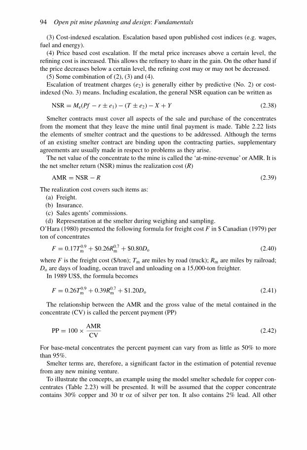
94 Open pit mine planning and design: Fundamentals
(3) Cost-indexed escalation. Escalation based upon published cost indices (e.g. wages,fuel and energy).(4) Price based cost escalation. If the metal price increases above a certain level, the
refining cost is increased. This allows the refinery to share in the gain. On the other hand ifthe price decreases below a certain level, the refining cost may or may not be decreased.(5) Some combination of (2), (3) and (4).Escalation of treatment charges (e2) is generally either by predictive (No. 2) or cost-
indexed (No. 3) means. Including escalation, the general NSR equation can be written as
NSR = Me(Pf − r ± e1) − (T ± e2) − X + Y (2.38)
Smelter contracts must cover all aspects of the sale and purchase of the concentratesfrom the moment that they leave the mine until final payment is made. Table 2.22 liststhe elements of smelter contract and the questions to be addressed. Although the termsof an existing smelter contract are binding upon the contracting parties, supplementaryagreements are usually made in respect to problems as they arise.The net value of the concentrate to the mine is called the ‘at-mine-revenue’ or AMR. It is
the net smelter return (NSR) minus the realization cost (R)
AMR = NSR − R (2.39)
The realization cost covers such items as:(a) Freight.(b) Insurance.(c) Sales agents’ commissions.(d) Representation at the smelter during weighing and sampling.
O’Hara (1980) presented the following formula for freight cost F in $ Canadian (1979) perton of concentrates
F = 0.17T 0.9m + $0.26R0.7
m + $0.80Do (2.40)
where F is the freight cost ($/ton); Tm are miles by road (truck); Rm are miles by railroad;Do are days of loading, ocean travel and unloading on a 15,000-ton freighter.
In 1989 US$, the formula becomes
F = 0.26T 0.9m + 0.39R0.7
m + $1.20Do (2.41)
The relationship between the AMR and the gross value of the metal contained in theconcentrate (CV) is called the percent payment (PP)
PP = 100 × AMR
CV(2.42)
For base-metal concentrates the percent payment can vary from as little as 50% to morethan 95%.Smelter terms are, therefore, a significant factor in the estimation of potential revenue
from any new mining venture.To illustrate the concepts, an example using the model smelter schedule for copper con-
centrates (Table 2.23) will be presented. It will be assumed that the copper concentratecontains 30% copper and 30 tr oz of silver per ton. It also contains 2% lead. All other

Mining revenues and costs 95
Table 2.22. The major elements of a smelter contract and the questions addressed (Werner & Janakiraman,1980).
1. The parties to the contract.Who is the seller andwho is the buyer?
2. The material and its quality.What is the natureof the material; for example, ore or concentrate?What are its assay characteristics and on whatbasis (wet or dry) are any assays made andreported?
3. The quantity and duration of the contract.What are the amounts involved? Are theshipments sent wet or dry? What is the size ofa lot? What is the duration of the contract andhow are the shipments to be spread out overthe period in question?
4. What is the mode of delivery.What is the modeof delivery (in bulk or otherwise)? In whatmanner is the shipment to be made and how is itto be spread over the life of the contract? Is it tobe delivered by truck, rail or ship and on whatbasis; for example, C.I.F. or F.O.B.? Which ofthe parties to the contract pays the transportationcharges?
5. The price to be paid. How much of the metalcontained in the shipment is to be paid for? Isthere any minimum deduction from the reportedcontent of the concentrate? What is the natureof the prices; for example, simple or weightedaverage? Which particular price or prices areto be used, for example; NewYork or LondonMetal Exchange basis, and in what publicationsare these prices published? What is quotationalperiod involved? How is the price derivedaveraged over what quotational period?
In what current is the price to be paid? Ifit is an average price, what is the basis forthe averaging? What forms of weightmeasurement are to be used: for example,troy, avoirdupois or metric? What premiums,if any, are to be offered? What are theprovisions if the quotation ceases to bepublished or no longer reflects the full value ofthe metal?
6. The smelter’s charges. What is the smelter’sbase charge for treatment? On what groundsmight it be increased or decreased, and if so,how might this be done – in relation to the priceof metal or to some other change such as avariation in the cost of labour at the smelter?What are the penalties or premiums for excessmoisture and for exceeding minimum ormaximum limits in content of other elementsof mineral constituents?
What are the associated refining charges,if any?
7. The quotational period.What is thequotational period (for example, thecalendar month following the month duringwhich the vessel reports to customs ata designated port) and how is thisspecified?
8. Settlement.Whose weights and samples areto be used and what represents a smelter lot?
9. Mode of payment. How much is to bepaid and when (for example, 80% of theestimated value of each smelter lot shall bepaid for at the latest two weeks after thearrival of the last car in each of thelot at buyers’ plant)?Where, in what form and how are the
payments to be made and what are theprovisions for the making of the finalpayment?
10. Freight allowances. Which party pays duties,import taxes, etc.?
11. Insurance. Which party pays for insuranceand to what point? For example, ‘alongsidewharf’.
12. Other conditions. What are the provisionsconcerning events beyond the control ofthe buyer or seller? When may ‘forcemajeure’ be invoked? What are theconditions under which the contract maybe assigned to a third party by the buyeror the seller? What, if any, are theprovisions in regard to the presenceof specific minor minerals or metals inthe concentrate?
13. Payment conversion rates.What pricequotations and currency conversion ratesare to be used and in what publication arethey quoted? What are the provisions forthe adoption of new bases if those usedcease to be published?
14. Arbitration.Where are any problems tobe arbitrated? How and under whatjurisdiction?
15. Weighing, sampling and moisturedetermination. Who does this,where, and who pays for it? Does the sellerhave the right to be represented at theprocedure at his own expense? How are thesamples taken to be distributed amongbuyer, seller and umpire?

96 Open pit mine planning and design: Fundamentals
Table 2.22. (Continued).
16. Assaying.What are the proceduresfor assaying? What is an acceptable assayfor settlement purposes and what arethe splitting limits? Which party pays forumpire assaying?
17. Definitions of terms.What are the agreed upondefinitions of terms? For example: ‘Shortton equivalent to 2000 poundsavoirdupois.’ Do dollars and centsrefer to, for example, Canadian orUnited States currency?
18. Insurance. What insurance coverageis required and which party is to pay for it?
19. Title.At what point shall title pass from sellerto buyer?
20. Risk of loss.At what point shall risk of losspass from seller to buyer?
21. Arbitration and jurisdiction. What are theprocedures for settling any disputesthat may arise between the parties andwhich country’s law are to govern theparties?
Table 2.23. Model 1989 smelter schedule for copper concentrates (Western Mine Engineering, 1989).
Payments copper Pay for 95% to 98% of the copper content at market value, minimumdeduction of 1.0 unit per dry ton for copper concentrates grading below30%. Unit deductions and treatment charges may be higher forconcentrates above 30% copper.
gold Deduct 0.02 to 0.03 troy ounce per dry ton and pay for 90% to 95%of the remaining gold content at market value.
silver Deduct 1.0 troy ounce per dry ton and pay for 95% of the remainingsilver content at market value.
Deductions treatmentcharge
$65 to $100 per dry ton ore or concentrate. Concentrates sold on thespot market are commanding a treatment charge of about $90 to$100 per short ton.
refining $5.00 to $6.00 per ounce of accountable gold.charges $0.30 to $0.40 per ounce of accountable silver.
$0.075 to $0.105 per pound of accountable copper, March, 1989 spotconcentrate deals are carrying refining charges of about $0.11 per pound,long term refining charges are usually $0.09 to $0.095 per pound.
Excessive amounts of some of the following elements may result in rejectionDeleteriouselement
lead Allow 1.0 units free; charge for excess at up to $10.00 per unit. (Nopenalty at some plants).
assessments zinc Allow 1.0 to 3.0 units free; charge for excess at up to $10.00 per unit.(No penalty at some plants).
arsenic Allow 0.0 units free; charge for excess at $10.00 per unit.antimony Allow 0.0 units free; charge for excess at $10.00 per unit.bismuth Allow 0.5 units free; charge for excess at $20.00 per unit.nickel Allow 0.3 units free; charge for excess at $10.00 per unit. (No penalty
at some plants).moisture Allow 10.0 units free; charge for excess at $1.00 per unit. (No penalty
at some plants).alumina Allow 3.0 units free; charge for excess at $1.00 per unit.other Possible charges for fluorine, chlorine, magnesium oxide, and mercury.
deleterious elements are below the allowable limits. Assumed prices are $1/lb for copper,$6/tr oz for silver and $0.50/lb for lead. The payments, deductions and assessments are:
PaymentsCopper: C = 98%
f = 1.0u = 1%

Mining revenues and costs 97
Silver: C = 95%f = 1.0u = 1.0 tr oz
DeductionsCopper: T = $75/ton
r = $0.10/lbSilver: r = $0.35/tr oz of accountable silver
AssessmentsLead: 1 unit is free
additional units charged at $10.00 per unit.The copper provides the major source of income. Using Equation (2.34) one finds that thebasic smelter return is
BSR = Me(Pf − r) − T
= C
100
G − u
1002000(Pf − r) − T
= 98
100
30 − 1
1002000($1 × 1 − 0.10) − $75
= $436.56/ton of concentrate
The penalty charge for excess lead is
X = is the (Units present − Units allowable) × Charge/unit
= (2 − 1)$10.00 = $10.00
The by-product credit for silver is
Y =(
C
100
)(G − u)(Pf − r)
=(
95
100
)(30.0 − 1.0)($6 × 1.0 − 0.35) = $155.66/ton of concentrate
Hence the net smelter return is
NSR = $436.56 − $10.00 + $155.66 = $582.22/ton of concentrate
It will be assumed that the concentrates are shipped 500 miles by rail to the smelter. Thetransport cost (F) per ton of concentrate is
F = 0.39R0.7m = 0.39(500)0.7 = $30.22
The at-mine-revenue becomes
AMR = $582.22 − $30.22 = $552
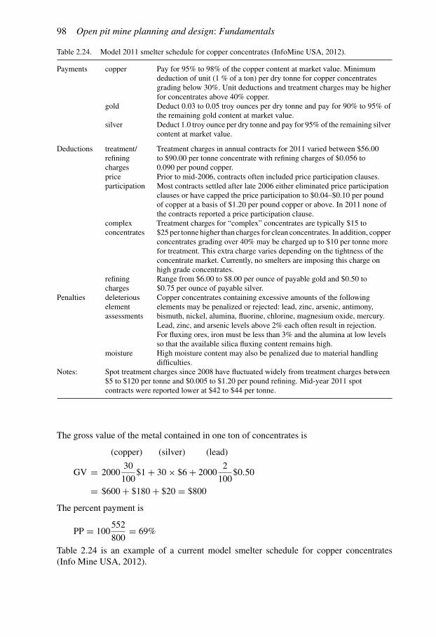
98 Open pit mine planning and design: Fundamentals
Table 2.24. Model 2011 smelter schedule for copper concentrates (InfoMine USA, 2012).
Payments copper Pay for 95% to 98% of the copper content at market value. Minimumdeduction of unit (1 % of a ton) per dry tonne for copper concentratesgrading below 30%. Unit deductions and treatment charges may be higherfor concentrates above 40% copper.
gold Deduct 0.03 to 0.05 troy ounces per dry tonne and pay for 90% to 95% ofthe remaining gold content at market value.
silver Deduct 1.0 troy ounce per dry tonne and pay for 95% of the remaining silvercontent at market value.
Deductions treatment/refiningcharges
Treatment charges in annual contracts for 2011 varied between $56.00to $90.00 per tonne concentrate with refining charges of $0.056 to0.090 per pound copper.
priceparticipation
Prior to mid-2006, contracts often included price participation clauses.Most contracts settled after late 2006 either eliminated price participationclauses or have capped the price participation to $0.04–$0.10 per poundof copper at a basis of $1.20 per pound copper or above. In 2011 none ofthe contracts reported a price participation clause.
complexconcentrates
Treatment charges for “complex” concentrates are typically $15 to$25 per tonne higher than charges for clean concentrates. In addition, copperconcentrates grading over 40% may be charged up to $10 per tonne morefor treatment. This extra charge varies depending on the tightness of theconcentrate market. Currently, no smelters are imposing this charge onhigh grade concentrates.
refiningcharges
Range from $6.00 to $8.00 per ounce of payable gold and $0.50 to$0.75 per ounce of payable silver.
Penalties deleteriouselementassessments
Copper concentrates containing excessive amounts of the followingelements may be penalized or rejected: lead, zinc, arsenic, antimony,bismuth, nickel, alumina, fluorine, chlorine, magnesium oxide, mercury.Lead, zinc, and arsenic levels above 2% each often result in rejection.For fluxing ores, iron must be less than 3% and the alumina at low levelsso that the available silica fluxing content remains high.
moisture High moisture content may also be penalized due to material handlingdifficulties.
Notes: Spot treatment charges since 2008 have fluctuated widely from treatment charges between$5 to $120 per tonne and $0.005 to $1.20 per pound refining. Mid-year 2011 spotcontracts were reported lower at $42 to $44 per tonne.
The gross value of the metal contained in one ton of concentrates is
(copper) (silver) (lead)
GV = 200030
100$1 + 30 × $6 + 2000
2
100$0.50
= $600 + $180 + $20 = $800
The percent payment is
PP = 100552
800= 69%
Table 2.24 is an example of a current model smelter schedule for copper concentrates(Info Mine USA, 2012).

Mining revenues and costs 99
2.3.6 Price-cost relationships
Using the net smelter return formula it is possible to calculate the revenue per ton of con-centrate. The revenue to the mine every year depends upon the tons of concentrate producedand the price. The costs to the mine on the other hand depend upon the amount of materialmined and processed.If one assumes thatK tons of concentrate are produced every year, then the yearly revenue
depends directly on the price received for the product.A large capital investment is required at the start of the mining. As will be discussed
later this must be recovered from the yearly profits. If the yearly profits are not as expected,then the payments cannot be made. Therefore it is important that the price projections orprice forecasts be made covering at least the depreciation period (that period in which theinvestment is being recovered).By examining the simplified net smelter return formula,
NSR = C
10020(G − u)
P − r
100− T (2.43)
where P is the price, r is the refining and selling cost, T is the treatment cost,G is the percentof metal, u is the fixed unit deduction (%), one can see that the revenue is equal to
k(P − r) − T − F
where k is a constant.Assume for definiteness that
C = 100%r = 12� cT = $60u = 1.3%G = 28.5%P = 90� c
Thus
NSR = 1 × 20(28.5 − 1.3)
(P − r
100
)− T = 544
100(P − r) − T
= 5.44(90 − 12) − 60 = $364.32
Assume that next year both the price and the costs increase by 5% but thatC,G and u remainconstant
P = 90 × 1.05 = 94.5� cr = 12 × 1.05 = 12.6� cT = 60 × 1.05 = $63
Hence
NSR = 5.44 × 81.9 − 63 = $382.54
The net present value would be
NPV = 382.54
1.05= $364.32

100 Open pit mine planning and design: Fundamentals
If the price however decreased by 5% and the costs increased by 5%, then
NSR = 5.44(85.5 − 12.6) − 63 = $333.58
If the price increased by 10% and the costs increased by 5%, then
NSR = 5.44(99 − 12.6) − 63 = $407.02
The conclusion is that the net smelter return depends upon the relative changes of the priceand the costs. If the prices and costs escalate at the same rate then the expected returnremains intact. If however, there is a difference then the return may be significantly more orsignificantly less than expected. Obviously the problem area is if the costs are significantlymore than expected or the price significantly less.
2.4 ESTIMATING COSTS
2.4.1 Types of costs
There are a number of different types of costs which are incurred in a mining operation(Pfleider &Weaton, 1968). There are also many ways in which they can be reported.Three cost categories might be:– Capital cost;– Operating cost;– General and administrative cost (G&A).
The capital cost in this case might refer to the investment required for the mine and millplant. The operating costs would reflect drilling, blasting, etc. costs incurred on a per tonbasis. The general and administrative cost might be a yearly charge. The G&A cost couldinclude one or more of the following:
– Area supervision;– Mine supervision;– Employee benefits;– Overtime premium;– Mine office expense;– Head office expense;– Mine surveying;– Pumping;– Development drilling;– Payroll taxes;– State and local taxes;– Insurance;– Assaying;– Mine plant depreciation.
The capital and G&A costs could be translated into a cost per ton basis just as the operatingcosts. The cost categories might then become:
– Ownership cost;– Production cost;– General and administrative costs.
The operating cost can be reported by the different unit operations:– Drilling;– Blasting;

Mining revenues and costs 101
– Loading;– Hauling;– Other.
The ‘other category’ could be broken down to include dozing, grading, road maintenance,dump maintenance, pumping, etc. Some mines include maintenance costs together with theoperating costs. Others might include it under G&A. Material cost can be further brokendown into components. For blasting this might mean:
– Explosive;– Caps;– Primers;– Downlines.
The operating cost could just as easily be broken down for example into the categories:– Labor;– Materials, expenses and power (MEP);– Other.
At a given operation, the labor expense may include only the direct labor (driller, anddriller helper, for example). At another the indirect labor (supervision, repair, etc.) could beincluded as well.There are certain costs which are regarded as ‘fixed’, or independent of the production
level. Other costs are ‘variable’, depending directly on production level. Still other costs aresomewhere in between.Costs can be charged against the ore, against the waste, or against both.For equipment the ownership cost is often broken down into depreciation and an average
annual investment cost. The average annual investment cost may include for example taxes,insurance and interest (the cost of money).The bottom line is that when discussing, calculating or presenting costs one must be very
careful to define what is meant and included (or not included). This section attempts topresent a number of ways in which costs of various types might be estimated.
2.4.2 Costs from actual operations
Sometimes it is possible to obtain actual costs from ‘similar’ operations. However greatcare must be exercised in using such costs since accounting practices vary widely. For manyyears theCanadianMining Journal has published its ‘ReferenceManual andBuyersGuide’.A great deal of useful information is contained regarding both mine and mill. Table 2.25contains information from the 1986 edition for the Similkameen Mine.Similar information for eleven open pit operations of different types and sizes as extracted
from the 1993 edition of the Reference Manual (SouthamMining Group, 1992), is includedin Table 2.26. Since SimilcoMines Ltd. is the successor of Similkameen Property describedin Table 2.25, one can examine changes in the operation and in the costs with time.Information as complete as this is seldom publicly available.The 2004 edition of the CMJ Mining Source book (CMJ, 2004) has included the detailed
cost information for the Huckleberry Mine given in Table 2.27. Operating and cost data forsome Canadian open pit mines published in the 2010 Mining Sourcebook (CMJ, 2010) arepresented in Table 2.28. The authors understand that the 2010Mining Sourcebook is the lastin a long series. This is unfortunate since it has been a very valuable resource. The authorsare grateful to the Canadian Mining Journal for permission to include this valuable set ofinformation.

102 Open pit mine planning and design: Fundamentals
Table 2.25. Cost information (Canadian $) for the Simikameen Mine,Newmont Mining Company Mines Limited (CMI, 1986).
1. Location: Princeton, British Columbia, Canada
2. Pit geometry(a) Pit size at surface: 3200′ × 1000′(b) Pit depth: 330′(c) Bench height: 40′(d) Bench face angle: 70◦(e) Berm width: 40′(f) Road grade: 10%
3. Capacity(a) Mining: ore= 22,000 tpd
Waste= 25,500 tpdore and waste= 5,111,500 tpy (actual)
(b) Milling: capacity= 20,000 tpdore= 2,945,000 tpy (actual)mill heads= 0.43% Cuminerals recovered=Cu, Au, Agrecovery= 85.5%concentrate grade= 30% Cuprincipal processes: primary SAG, secondarycone crusher, ball milling, Cu flotation
4. Pit equipment(a) Ore and waste loading= 4 P & H 1900A shovels (10 yd3)(b) Ore and waste haulage= 15 Lectra Haul M100 trucks(c) Other= 4 Cat D8K dozers
1 Cat 14E grader3 Cat 824 r.t.d.1 Dart 600C f.e.l. (15 yd3)2 Komatsu 705A graders
5. Blasting in ore and waste(a) Explosives 85% bulk Anfo
15% packaged slurry(b) Powder factor (lb/ton)= 0.46(c) Loading factor (lb/yd3)= 0.70
6. Drilling in ore and waste(a) Drills= 3 Bucyrus-Erie 60R(b) Hole diameter= 97/8′′(c) Pattern (burden × spacing)= 18′× 24′(d) Feet drilled/shift= 490′(e) Tons/foot= 26(f) Bit life= 6,000 ft(g) Rod life= 320,000 ft
7. Power requirements(a) Total (all motors)= 53,600 HP(b) Peak demand= 35,776 kVA(c) Annual mill demand= 255,282,172 kWh(d) Total annual demand= 266,573,172 kWh
(Continued)

Mining revenues and costs 103
Table 2.25. (Continued).
8. Personnel(a) Open pit
Staff personnel 20Equipment operators, labor 78Mechanical, maintenance crew 44___
Total open pit workforce 142(b) Mineral processing plant
Staff personnel 25Operators (all classifications) 37Repair and maintenance crew 45___
Total mill workforce 107(c) Surface plant
Staff personnel 1Mechanical and maintenance crew 13___
Total surface plant workforce 14(d) Other
Office and clerical personnel 22Warehouse 14___
Total other 36_______________________________________________________
Total employees 299
9. Mining costs for ore and waste ($/ton)(a) Dozing and grading 0.05(b) Drilling 0.07(c) Blasting 0.13(d) Loading 0.14(e) Hauling 0.21(f) Crushing 0.11(g) Conveying 0.06(h) Pumping 0.01(i) Maintenance 0.10(j) Supervision 0.02(k) Other 0.02_________________________________________________________
Total $0.92
10. Milling costs ($/ton)(a) Crushing 0.096(b) Grinding 1.844(c) Flotation 0.244(d) Drying 0.075(e) Assaying 0.015(f) Conveying 0.091(g) Power 0.921(h) Tailings disposal 0.137(i) Labor 0.437(j) Supervision 0.094______________________________________________________
Total $3.954

104Open
pitmine
planningand
design:Fundam
entals
Table 2.26. Operating and cost data from some Canadian open pit mines (Southam Mining Group, 1993).
1. Open pit mines included

Mining
revenuesand
costs105
2. Deposit description
(Continued)

106Open
pitmine
planningand
design:Fundam
entals
Table 2.26. (Continued).
3. Pit equipment

Mining
revenuesand
costs107
4. Drilling equipment and practices
(Continued)

108Open
pitmine
planningand
design:Fundam
entals
Table 2.26. (Continued).
5. Blasting practices

Mining
revenuesand
costs109
6. Primary crushing
(Continued)

110Open
pitmine
planningand
design:Fundam
entals
Table 2.26. (Continued).
7. Mineral processing

Mining
revenuesand
costs111
8. Personnel numbers and distribution
1Warehouse and safety personnel. 2Employees of contractor.
(Continued)

112Open
pitmine
planningand
design:Fundam
entals
Table 2.26. (Continued).
9. Mine operating costs (Canadian $/ton)
*Amounts reported in metric units have been converted to imperial equivalents. 1Includes conveying. 2Includes reclamation $0.055, mine shipping expense$0.096, and other $0.089. 3Includes loading. 4Supervision. 5Includes blasting. 6Includes engineering and geology.

Mining
revenuesand
costs113
10. Processing costs (Canadian $/ton)
*Amounts reported in metric units have been converted to imperial equivalents. 1Includes grinding balls $0.480, mill liners $0.160, fuel and lubricants $0.008,and operating supplies $0.046.

114 Open pit mine planning and design: Fundamentals
Table 2.27. Cost information (Canadian $) for the Huckleberry Mine (CMJ, 2004).
1. Location: Houston, British Columbia, Canada
2. Pit geometry(a) Pit size at surface: 1050m× 600m(b) Pit depth: 320m(c) Bench height: 12m(d) Bench face angle: 70◦(e) Berm width: 10m(f) Road grade: 10%(g) Slope angle: 52◦
3. Capacity(a) Mining: ore = 21,000 mtpd
waste= 44,000 mtpdore and waste= 19,034,000 tonnes (actual)
(b) Milling: capacity= 20,333 mtpd(c) ore= 7,422,000 tonnes (actual)
mill heads= 0.534% Cu, 0.014% Mominerals recovered=Cu, Morecovery= 88.38% Cu, 47.54% Moconcentrate grade = 27.19% Cu, 48.73% Moprincipal processes: SAG & ball milling, bulk float,
regrinding & dewatering, Moly float, Cu-Moseparation, float and regrinding.
4. Pit equipment(a) Ore and waste loading= 1 P&H 1900AL shovel
1 P&H 2100BL shovel1 Cat 992C FEL1 Cat 416
(b) Ore and waste haulage= 5 Cat 777C trucks4 Cat 785B trucks1 Cat 777B truck
(c) Other= 2 Cat D9N dozers2 Cat D8N dozers1 Cat D10N dozer1 Cat 824 RTD2 Cat 16G graders1 Hitachi excavator1 Cat 769 water truck
5. Blasting in ore and waste(a) Emulsion(b) Powder factor (kg/t)= 0.20(c) Loading factor (kg/m3)= 0.54
6. Drilling in ore and waste(a) Drills= 2 Bucyrus-Erie 60R(b) Hole diameter= 251mm(c) Pattern (burden × spacing)= 7.5m× 7.5m to 9.3m× 9.3m offset & wall control(d) Drilling per shift = 140m(e) Tons/m= 177(f) Bit life= 2227 m(g) Rod life=NA
(Continued)

Mining revenues and costs 115
Table 2.27. (Contined).
7. Power requirements(a) Total (all motors)= 190,900,000 kWh(b) Peak demand= 30 kVA(c) Annual mill demand= 190,500,000 kWh(d) Total annual demand= 195,300,000 kWh
8. Personnel(a) Open pit
Staff personnel 18Equipment operators, labor 68Mechanical, maintenance crew 34___Total open pit workforce 120
(b) Mineral processing plantStaff personnel 12Operators (all classifications) 33Repair and maintenance crew 12___Total mill workforce 68
(c) OtherOffice and clerical personnel 14Others 9___Total other 23__________________________________________Total employees 211
9. Mining costs for ore and waste ($/tonne)(a) Dozing and grading 0.158(b) Drilling 0.053(c) Blasting 0.111(d) Loading 0.221(e) Hauling 0.210(f) Crushing incl(g) Conveying incl(h) Pumping 0.024(i) Maintenance incl(j) Supervision and labor incl(k) Power incl(l) Other 0.135___________________________________________
Total $1.123
10. Milling costs ($/tonne)(a) Crushing 0.269(b) Grinding 1.940(c) Reagents 0.009(d) Flotation 0.545(e) Dewatering 0.122(f) Tailings disposal 0.056(g) Assaying 0.047(h) Conveying 0.091(i) Power incl(j) Supervision & labor incl(k) Maintenance incl(l) Other 0.359___________________________________________
Total $3.342

116Open
pitmine
planningand
design:Fundam
entals
Table 2.28. Operating and cost data from some Canadian open pit mines (CMJ, 2010).
1. Open pit mines included
Company, Mine Location Minerals recovered Pit size (L×W×D) Ore mined Waste Removed
ArcelorMittal, Mt-Wright Fermont, QC Fe
Barrick, Williams Hemlo, ON Au 1100 × 600 × 230m 5,000 t/d 18,000 t/d
BHP Diamonds, Ekati Lac des Gras, NT Diamonds 7,000 t/d 115,000 t/d
Highland Valley Copper Logan Lake, BC Bornite, Chalcopyrite,Molybdenite
Lornex: 2100× 700× 540mValley: 1400× 1000× 700m
124,300 t/d 40,800 t/d
Huckelberry Mines Houston, BC Cu, Au, Ag, Mo 1050× 600× 320m 19,500 t/d 20,100 t/d
Imperial Metals, Mount Polley Likely, BC Cu, Au, Ag Wight pit: 800× 380× 200mBell pit: 650× 400× 170mSpringer pit: 1100× 800× 400mSE pit: 300× 250× 100mC2 pit: 620× 300× 130m
20,000 t/d 76,000 t/d
Inmet, Troilus Chibougamau, QC Au, Cu 1100× 500m1300× 275m
20,000 t/d 35,000 t/d
Iron Ore, Carol Labrador City, NL Hematite & magnetite 910× 3000× 200m 110,000 t/d 11,000 m3/d
Northgate, Kemess Smithers, BC Au, Cu, Ag 1800× 900× 390m 49,700 t/d 52,000 t/d
Thompson Creek, Endako Endako, BC Mo 2000× 760× 260m 28,500 t/d 28,500 t/d max
Xstrata Nickel, Spoon Nunavik, QC Ni, Cu 200× 145× 40m 750 t/d 2,300 t/d

Mining
revenuesand
costs117
2. Deposit description
Company, Mine Proven & probable In-situ grade Ore Typereserves
ArcelorMittal, Mt-Wright
Barrick, Williams 13.2 million tonnes 1.80 g/t Au Replacement type late hydrothermal mineralization along fracturesystems mostly subparallel to foliation
BHP Diamonds, Ekati 1.90 carat/tonne Kimberlite
Highland Valley Copper 494 million tonnes 0.381% Cu0.0073% Mo
Lornex: Sulphide in fracture fillingValley: Sulphide
Huckelberry Mines 19.4 million tonnes 0.529% Cu0.015% Mo0.059 g/t Au2.982 g/t Ag
Quartz & sericite veins Porphyry Cu-Mo stockworks & disseminationsof Chalcopyrite & molybdenite
Imperial Metals, Mount Polley 55.6 million tonnes 0.357% Cu0.298 g/t Au0.661 g/t Ag
Alkalic Cu-Au porphyry
Inmet, Troilus 27.6 million tonnes 0.83 g/t Au0.08% Cu
Iron Ore, Carol 5,300 million tonnes 38.6% Fe Iron formation
Northgate, Kemess 34.2 million tonnes 0.17% Cu0.41 g/t Au
Porphyry Cu-Au
Thompson Creek, Endako 0.074% Mo Porphyry style veined quartz molybdenum stockwork
Xstrata Nickel, Spoon 157,250 tonnes 3.16% Ni
(Continued)

118Open
pitmine
planningand
design:Fundam
entals
Table 2.28. (Continued).
3. Pit equipment
Company, Mine Ore, waste or other Shovels Loaders Trucks
ArcelorMittal, Mt-Wright 1 P&H 23004 Bucyrus-Erie BII1 Bucyrus-Erie HR1 Demag
4 Letourneau L1800 10 Cat 793, 240-t20 Cat 789,190-t
Barrick, Williams Ore & waste 2 Cat 992G 6 Cat 777, 80-t
BHP Diamonds, Ekati Kimberlite & other 1 Cat 531 excavator3 Komatsu PC 1800 excavator
1 Cat 992D, 12,000 t/d 10 Cat 777D, 90-t
Waste & other 2 Demag 655SP3 Komatsu PC 1800 excavator
1 Cat 994C, 21,400 t/d1 Cat 994C, 12,000 t/d
13 Cat 793C, 218-t3 Cat 789C, 180-t
Highland Valley Copper Ore & waste 2 P&H 2800XP/B, 31.3m3
2 P&H 2800XP/A, 31.3m3
1 Bucyrus-Erie 295,16.8m3
2 Bucyrus 495 42m3
2 Letourneau L1850, 21.4m3
1 Letourneau L1400, 21.4m317 Cat 789, 172-t38 Cat 793, 225-t
Huckleberry Mines Ore & waste 1 P&H 1900AL2 P8H 2100BL
1 Cat 992C1 Cat 416
5 Cat 777C4 Cat 785B1 Cat 777B
Imperial Metals, Mount Polley Ore & waste 1 P8H 2100 electric, 13.75m3
3 P8H 2100 electric, 12.5m31 Cat 992C, 9m3
1 Hitachi 1100, 3.5m3
1 Komatsu 1800, 12m3
2 Cat 777B, 86-t3 Cat 777C, 86-t2 Cat 777D, 90-t11 Cat 785C, 140-t1 Cat 785D, 140-t
Inmet, Troilus Ore & waste 2 Demag H285 hyd, 16.8m3 1 Letourneau L1100, 16.8m3 9 Cat 7858,150-t
Iron Ore, Carol Ore & waste 2 P&H 2800XPB, 32m3
4 Bucyrus-Erie 295BII, 18m31 Letourneau 1800,15.3m3
1 Letourneau 1100,11.5m315 Komatsu 830E, 227-t
Northgate, Kemess Ore & waste 1 P&H 2800 XPB, 35.1 m3
1 P&H 2300 XPB, 25.2m3
1 Hitachi EX5500 hyd, 26.8m3
1 Letourneau L1400, 21.4m3 15 Euclid 260, 240-t
Thompson Creek, Endako Ore & waste 1 P&H 2100XP, 14.5m3
1 Bucyrus-Erie 290B, 14.5m3
1 P&H 280DD, 33.6m3
1 P8H 4100BL, 9.9m3
1 Cat 980C1 Cat 690D1 Cat 996D1 Cat 992
9 Euclid R1902 Unit Rig M120
Xstrata Nickel, Spoon Ore & waste 1 Hitachi EX450, 3.8m3
1 Hitachi EX11001 John Deer 60C CL
2 Cat 988, 11.4-t1 Cat 980, 4- 6m3
1 Cat 966, 3.4 - 4.2m3
8 Cat 769, 35-t4 Mac CV713, 30-t

Mining
revenuesand
costs119
4. Drilling & Blasting
Company, Mine Blasthole drills Holediameter
Holepattern
Explosives
Ore/waste Type Loadingfactor
BHP Diamonds, Ekati 3 Tamrock DK90 diesel2 Ingersoll-Rand DM45HP1 Driltech D45S
265mm265mm265mm
6.5× 6.5m6.5× 6.5m6.5× 6.5m
KimberliteWaste
Anfo-bulk emulsionAnfo-bulk emulsion
Highland Valley Copper 4 Bucyrus-Erie 49R1/111 Prod’n: 310mmWalls. 270mm
Ore Waste 0.51 kg/t0.47 kg/t
Huckleberry Mines 2 Bucyrus-Erie 60 R 251mm 7.5× 7.5m to9.3× 9.3m
Ore Emulsion 048 kg/m3
Imperial Metals, Mount Polley 1 Bucyrus-Erie 45R2 Bucyrus-Erie 60R1 Driltech C40K DDH1 Pit Viper 351
250mm250mm165mm310mm
7.4× 8.5m7.× 8.5m6× 6m7.9× 9.1m
Ore WasteOre
SuperAn (same as ore)Apex Gold
0.56 kg/t0.47 kg/t
Inmet, Troilus 3 lngersoll-Rand DML60 170 & 190mm 5.5× 5.5m Ore & waste Emulsion
Iron Ore, Carol 1 Gardner Denver 1204 Bucyrus-Erie 49R
380mm 7.8× 7.8m &8× 8m
Northgate, Kemess 1 P8H 100 rotary
1 Ingersoll-Rand Pit Viper
3 Atlas Copco CM789D1 Air Trak
311mm
270 & 310mm
115 &130mm51mm
Ore Waste
Ore
Ore
BLX emulsion &Anfo(same as ore)BLX heavy Anfo &emulsionBLX heavy Anfo &emulsion
0.55 kg/m3
0.55 kg/m3
Thompson Creek, Endako Marion 4Gardner Denver 100Gardner Denver 120
315mm 7.9× 9.1m Ore & waste Fragmax & Fragmite 0.72 kg/m3
Xstrata Nickel, Spoon (owned by contractor) 140mm 4× 4m Ore Waste EmulsionEmulsion
1.17 kg/m3
1.13 kg/m3
(Continued)

120Open
pitmine
planningand
design:Fundam
entals
Table 2.28. (Continued).
5. Primary Crushing
Company, Mine Crusher site Crusher Crusher setting Transport & distance from crusherto mill
ArcelorMittal, Mt-Wright 2 gyratory
Barrick, Williams Outside pit A-C gyratory 170mm Crusher to stockpile: Conveyor, 450mStockpile to mill: Truck, 450m
BHP Diamonds, Ekati At plant Fuller 4270 gyratory 200mm Conveyor, 192m
Highland Valley Copper Lornex: Pit rimValley: In pit
1 A-C gyratory2 A-C gyratorysemi-mobile Krupp carrier
152mm152mm
Trucks, 2500mTrucks, 850m
Huckelberry Mines At mill Allis-Chalmers gyratory 150mm Conveyor, 280m
Imperial Metals, Mount Polley At mill Allis-Chalmers 260mm 1.5 to 4 km
Inmet, Troilus At mill Allis-Chalmers gyratory 150mm 250m
Iron Ore, Carol At mill 2 Allis-Chalmers gyratory 150mm 1800m
Northgate, Kemess At mill 1 Metso gyratory 150–200mm Trucks, 3790m
Thompson Creek, Endako In pit Kobello Allis-Chalmers 205mm Conveyor, 792m

Mining
revenuesand
costs121
6. Mineral Processing
Company, Mine Daily throughput Products Mill heads Recovery Concentrategrade
Principal processes
ArcelorMittal, Mt-Wright Autogenous grinding, spiral gravityconcentration & load out
Barrick, Williams 9085 tonnes Au bullion(84%Au& 10%Ag)
4.03 g/t Au 94.2% SAG, ball & vertical milling withgravity extraction, thickening,leaching & CIP, carbon stripping,electrowinning & refining
BHP Diamonds, Ekati 12,700 tonnes Diamonds 100% 1 carat/t Crushing, scrubbing, screening heavymedia separation & x-ray recovery
Highland Valley Copper 116,694 tonnes Cu conc 0.373% Cu 87.88% Cu 41.6% Cu 3 SAG lines with 2 closed-circuit ballmills each, 2 autogenous lines with1 closed-circuit ball mill & pebblecrusher each, bulk float of Cu-Moconc, diff Cu-Mo float, vacuum discfiltration & rotary gas-fired drying ofCu conc.
Mo conc 0.0068% Mo 62.7% Mo 51.8% Mo Ferric chloride leach of Mo float conc,pressure filtering & drying
Huckelberry Mines 19,822 tonnes Cu conc 0.555% Cu 88% Cu 27.38% Cu SAG & ball milling, bulk float,regrinding & dewatering
Mo conc 0.014% Mo 29% Mo 44.95% Mo Moly float, Cu-Mo separation, float ®rinding.
Imperial Metals,Mount Polley
20,000 tonnes Cu-Au-Agconc
0.57% Cu0.345 g/t Au2.543 g/t Ag
≈76%all metals
24.67% Cu14.39 g/t Au106.71 g/t Ag
Conventional grinding& bulk flotation
(Continued)
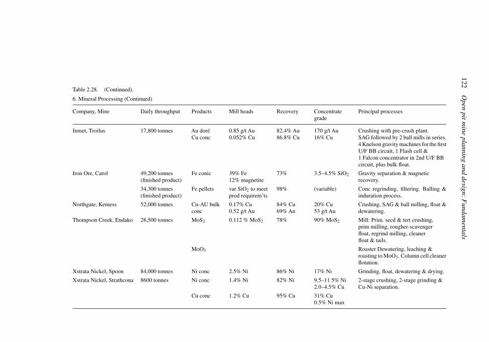
122Open
pitmine
planningand
design:Fundam
entals
Table 2.28. (Continued).
6. Mineral Processing (Continued)
Company, Mine Daily throughput Products Mill heads Recovery Concentrategrade
Principal processes
Inmet, Troilus 17,800 tonnes Au doréCu conc
0.85 g/t Au0.052% Cu
82.4%Au86.8% Cu
170 g/t Au16% Cu
Crushing with pre-crush plant.SAG followed by 2 ball mills in series.4Knelson gravitymachines for the firstU/F BB circuit, 1 Flash cell &1 Falcon concentrator in 2nd U/F BBcircuit, plus bulk float.
Iron Ore, Carol 49,200 tonnes(finished product)
Fe conic 39% Fe12% magnetite
73% 3.5–4.5% SiO2 Gravity separation & magneticrecovery.
34,300 tonnes(finished product)
Fe pellets var SiO2 to meetprod requirem’ts
98% (variable) Conc regrinding, filtering. Balling &induration process.
Northgate, Kemess 52,000 tonnes Cu-AU bulkconc
0.17% Cu0.52 g/t Au
84% Cu69%An
20% Cu53 g/t Au
Crushing, SAG & ball milling, float &dewatering.
Thompson Creek, Endako 28,500 tonnes MoS2 0.112 % MoS2 78% 90% MoS2 Mill: Prim. secd & tert crushing,prim milling, rougher-scavengerfloat, regrind milling, cleanerfloat & tails.
MoO3 Roaster Dewatering, leaching &roasting toMoO3. Column cell cleanerflotation.
Xstrata Nickel, Spoon 84,000 tonnes Ni conc 2.5% Ni 86% Ni 17% Ni Grinding, float, dewatering & drying.
Xstrata Nickel, Strathcona 8600 tonnes Ni conc 1.4% Ni 82% Ni 9.5–11 5% Ni2.0–4.5% Cu
2-stage crushing, 2-stage grinding &Cu-Ni separation.
Cu conc 1.2% Cu 95% Cu 31% Cu0.5% Ni max

Mining
revenuesand
costs123
7. Personnel numbers and distribution
Company, Mine Underground Open Pit Mineral Processing Engineering Geology Environment Health Office Other TotalEmployees Employees & safety & clerical workers
Employees Contractors on site
Barrick, Williams 203 53 55 29 147 487
BHP Diamonds, 430 645 189 25 6 34 20 81 358 1788Ekati
Highland Valley 496 420 132 1048Copper
Huckelberry Mines 115 71 7 1 1 1 13 209
Imperial Metals, 98 11 4 3 5 4 3 5 28 386Mount Polley
Northgate, Kemess 200 116 8 3 3 7 18 16 371
Thompson Creek, 455 113 101 17 24 243Endako
(Continued)

124Open
pitmine
planningand
design:Fundam
entals
Table 2.28. (Continued).
8. Estimated operating costs.
Company, Operation Mineralsrecovered
Unit cost Undergroundmining cost/t
Open pitmining cost/t
Mineralproces.cost/t
G &A Totaloperatingcost/t
source year
Abacus, Afton-Ajax Cu-Au $1.50 $3.76 $0.90 43-101 2009
Anaconda Mining,Pine Cove
Au $5.92 $1.57 $1.47 43-101 2005
Apollo Gold, Black Fox Au $387/oz Au $53.39 (ore) $2.13 (ore) $31.17 $75.40 (ore) FS 2008
Atlantic Gold,Touquoy
Au $5.52 (ore) $9.44 $16.37 Eng &cost est
2007
Detour Gold,Detour Lake
Au $1.75 (ore)$1.50 (waste)
$8.25 $12.00 FS 2008
Fortune Minerals,Sue-Dianne
Cu-Ag $2.59 (ore &waste)
$14.00 43-101 2008
Getty Cooper,Getty North & South
Cu-Mo $1.60 ore &waste
$12.94 $0.76/t $19.47 PFS 2009
Highland Valley,Highland Valley
Cu $2.82 (ore) $4.02 $7.30 43-101 2007
Imperial Metals,Mount Polley
Cu-Au $2.40 $3.61 $4.24 43-101 2004
Inmet, Troilus Cu-Au $13.00 Presentation 2008
InternationalWayside, OR
Au $17.50–$18.00 $4.85 (ore)$3.37 (waste)
$17.53 PEA 2007
Marathon PGM,Marathon
PGM-Cu $7.37 $6.02 $1.11 $14.50 FS 2009
Mustang Minerals,Mayville
Ni-Cu $2.50 (ore) $10.00 $5.00 $17.50 43-101 2006
Northgate, Kemess Cu-Au $2.32 $4.10 $13.18 Presentation 2009
Northgate,Young-Davidson
Au US$333/oz Au $20.74 (ore) $3.09 $10.20 $2.65 PFS 2009

Mining
revenuesand
costs125
8. Estimated operating costs. (Continued)
Company, Operation Mineralsrecovered
Unit cost Undergroundmining cost/t
Open pitmining cost/t
Mineralproces.cost/t
G &A Totaloperatingcost/t
source year
Osisko,Canadian Malartic
Au $319/oz Au $1.52 $3.27 $0.60/t FS 2008
Rainy River,Rainy River
Au $50.00 $1.00 $7.00 $1.25/t pit$7.50/tUG
43-101 2009
Shore Gold,Orion South
Diamonds $1.60 $3.29 $1.65 43-101 2009
Shore Gold, Star Diamonds $6.29 ore $3.29 $1.65/t $15.88 PFS 2009
Starfield,Ferguson Lake
Ni-Cu $49.98 (ore) $2.88 (moved) $18.89 $7.89 $84.54 2008
Taseko, Gibraltar Cu-Mo $3.41 ore $2.24 $6.15 43-101 2007
Taseko, Prosperity Cu-Au $2.27 $3.55 $6.26 FS 2007
Terrane,Mount Milligan
Cu-Au US$0.17/lb CuUS$51/oz Au LOM
$2.35 $3.89 $0.57 $6.96 FS 2009
Thompson Creek,Endako
Cu-Mo $0.69+Var. haulage
$4.45 43-101 2007
Victory Nickel, Minago Ni US$3.09/lb Ni $5.12 $8.86 $9.87 $0.87 $40.96 PEA 2006
Western Copper,Camacks
Cu-Au US$0.98/lb Ni $9.98 $7.64 $19.22(LOM)
FS 2007
Western Copper,Casino
Cu-Au $3.24 $6.01 $0.47 $9.72 PFS 2008
Western Troy,MacLeod Lake
Cu-Mo US$470/oz Ni $7.06 $9.39 $157.90 PEA 2008
Notes:In section 1, only open pit metal mines are included. Mines producing coal or oil sands are not included.For sections 2 through 7, only data from the mines listed in section 1 are included.Section 8, includes all open pit metal mines. Many were not listed in section 1. Some also have underground operations.The estimated costs in section 8 are not as detailed as those costs included in section 9, of older versions of the Sourcebook.

126 Open pit mine planning and design: Fundamentals
2.4.3 Escalation of older costs
Publications from years past often contain valuable cost information. Is there some simpletechnique for updating so that these costs could be applied for estimating even today? Theanswer is a qualified yes. The qualification will be discussed later in this section. Theprocedure involves the escalation of costs through the application of various publishedindexes. Table 2.29 is an example of the:
– Construction cost;– Building cost;– Skilled labor;– Common labor;– Materials.
Table 2.29. ENR cost indices (Engineering News Record (ENR), 2012).
Year Construction Cost Building Cost Skilled Labor Common Labor Materials
1976 2499 1425 2136 4700 10551977 2577 1545 2264 4977 11591978 2776 1674 2405 5303 12891979 3003 1819 2564 5676 14271980 3237 1941 2767 6168 14881981 3535 2097 3025 6802 15271982 3825 2234 3358 7545 15481983 4066 2384 3591 8020 16511984 4146 2417 3721 8269 16211985 4182 2425 3778 8396 16171986 4295 2483 3867 8616 16341987 4406 2541 3986 8869 16591988 4519 2598 4085 9120 16941989 4615 2634 4174 9381 16931990 4732 2702 4310 9646 17201991 4835 2751 4457 9935 17091992 4985 2834 4580 10243 17611993 5210 2996 4703 10525 19531994 5408 3111 4818 10856 20681995 5471 3112 4943 11146 19931996 5620 3203 5085 11444 20461997 5826 3364 5229 11697 22261998 5920 3391 5374 12024 21791999 6059 3456 5537 12383 21842000 6221 3539 5740 12790 21952001 6343 3574 5965 13242 21132002 6538 3623 6208 13871 20442003 6694 3693 6496 14386 19812004 7115 3984 6747 14978 22962005 7446 4205 7035 15555 24762006 7751 4369 7274 16164 25952007 7966 4485 7604 16756 25802008 8310 4691 7902 17415 27302009 8570 4769 8197 18190 26742010 8799 4883 8483 18776 26842011 9070 5058 8712 19257 2826

Mining revenues and costs 127
indices publishedweekly in theEngineeringNews Record (ENR). The average yearly valuesare given except where noted. To illustrate the application of the index system, assume thatthe cost of the mine maintenance building was $100,000 in June of 1978. The estimatedcost of the same building in June of 1989 would be
Cost June 1989 = Cost June 1978 × Building cost index (June 1989)
Building cost index (June 1978)
In this case
Cost June 1989 = 100,000 × 2626
1664= 100,000 × 1.58 = $158,000
The escalation factor of 1.58 is the ratio of the index values for the years involved. In asimilar way one can compute the escalation factors for the other ENR indexes over thisperiod. They are summarized below:
Construction cost factor = 4568
2754= 1.67
Building cost factor = 2626
1664= 1.58
Skilled labor factor = 4166
2376= 1.75
Common labor factor = 9336
5241= 1.78
Materials factor = 1686
1229= 1.37
Other indexes are also available. Table 2.30 gives the average hourly earnings for miningproduction/non supervisory workers as published by the U.S. Bureau of Labor Statistics(BLS) over the period 1964 through 2002. These values can also serve as a labor costescalator. For the period 1978 to 1989 the factor would be
Mining hourly wage factor = 13.25
7.67= 1.73
Table 2.31 gives average hourly earnings broken down by industry. Contained with thepublication Statistical Abstract of the United States are values for the producer price indexfor construction machinery and equipment. The values for the time period 1978 to 1991 aregiven in Table 2.32. The resulting factor for the 1978 to 2004 time period is
Construction machinery and equipment factor = 117.2
67.7= 1.73
Considering the five ENR indices plus the two from the BLS, an average escalationfactor of 1.71 is selected. The average cost inflation rate r over this 11 year period iscomputed by
(1 + r)11 = 1.71
Hence
r = 0.050
The rate is 5%/year.

128 Open pit mine planning and design: Fundamentals
Table 2.30. Average hourly wage of production workers broken down by industry using the SIC base(BLS, 2004).
Year Average hourly earnings ($/hr)
Mining∗ Metal Iron Copper Coal Bitum. Coal/ Nonmetallic Crushed/mining ores ores mining lignite minerals∗ broken stone
1964 $2.81 2.96 3.13 3.04 3.26 3.30 2.48 2.411965 2.92 3.06 3.16 3.15 3.45 3.49 2.57 2.471966 3.05 3.17 3.28 3.22 3.63 3.66 2.70 2.611967 3.19 3.24 3.30 3.26 3.73 3.76 2.85 2.721968 3.35 3.42 3.47 3.44 3.83 3.86 3.04 2.931969 3.60 3.64 3.70 3.65 4.20 4.24 3.27 3.211970 3.85 3.88 3.90 3.93 4.54 4.58 3.47 3.391971 4.06 4.12 4.19 4.16 4.78 4.83 3.70 3.641972 4.44 4.56 4.60 4.64 5.27 5.31 3.95 3.941973 4.75 4.84 4.88 4.90 5.70 5.75 4.22 4.211974 5.23 5.44 5.53 5.54 6.22 6.26 4.50 4.491975 5.95 6.13 6.29 6.36 7.21 7.24 4.95 4.841976 6.46 6.76 7.04 7.04 7.74 7.77 5.36 5.201977 6.94 7.28 7.49 7.49 8.25 8.27 5.81 5.671978 7.67 8.23 8.48 8.46 9.51 9.55 6.33 6.141979 8.49 9.27 9.57 9.53 10.28 10.31 6.90 6.621980 9.17 10.26 10.95 10.61 10.86 10.90 7.52 7.161981 10.04 11.55 12.16 11.83 11.91 11.95 8.28 7.931982 10.77 12.31 12.97 12.53 12.69 12.73 8.90 8.531983 11.28 12.58 12.39 13.10 13.73 13.78 9.31 8.701984 11.63 13.05 12.74 13.56 14.82 14.87 9.87 9.261985 11.98 13.38 13.01 13.62 15.24 15.3 10.18 9.591986 12.46 13.19 13.88 12.29 15.40 15.46 10.38 9.801987 12.54 12.94 14.36 11.42 15.76 15.81 10.60 10.001988 12.80 13.24 14.19 11.62 16.06 16.26 10.94 10.371989 13.25 13.58 14.24 11.80 16.26 16.39 11.25 10.691990 13.69 14.05 14.59 12.48 16.71 16.85 11.58 11.071991 14.21 14.87 16.36 13.36 17.06 17.21 11.93 11.241992 14.54 15.26 16.52 13.83 17.15 17.29 12.26 11.551993 14.60 15.29 16.67 14.03 17.27 17.46 12.70 12.011994 14.88 16.08 17.87 14.31 17.76 17.97 13.11 12.471995 15.30 16.77 18.49 14.93 18.45 18.70 13.39 12.661996 15.62 17.35 18.70 15.72 18.74 19.03 13.75 13.151997 16.15 17.82 18.85 16.32 19.01 19.30 14.19 13.561998 16.91 18.24 19.90 16.53 19.17 19.43 14.67 14.031999 17.05 18.26 20.43 16.18 19.15 19.33 14.97 14.472000 17.22 18.60 21.48 15.65 19.09 19.20 15.28 14.832001 17.56 18.74 21.63 15.77 18.94 19.05 15.62 15.022002 17.77 18.81 21.93 16.02 19.64 19.77 15.99 15.49
∗Except fuelsBLS, 2005. Employment, Hours, and Earnings from the Current Employment Statistics Survey(National) SIC.Series Reports EEU10000006, EEU10100006, EEU10101006, EEU10102006, EEU10120006,EEU10122006, EEU10140006, EEU10142006http://www.bls.gov/data/
It was indicated earlier that such escalation has to be done with some care.Amajor reasonfor this is the change in labor productivity which has occurred over time.Productivity is a very important aspect of cost estimation. It deals with the rate at which
a certain task can be accomplished. If for example the daily production for a one shift per

Mining revenues and costs 129
Table 2.31. Average hourly earnings of production workers using the NAICS base (BLS, 2012a).
Year Average hourly earnings ($/hr)
Mining* Coal Metal Ore Nonmetallic Mineral Bituminous coal/LigniteMining Mining Mining and Quarryings surface mining
1990 15.47 18.42 15.19 11.81 11.821991 15.96 18.79 16.15 12.15 12.161992 16.11 18.86 16.50 12.50 12.521993 16.08 18.96 16.53 12.95 12.971994 16.67 19.52 17.40 13.36 13.371995 17.15 20.32 18.17 13.64 13.661996 17.51 20.70 18.77 14.05 14.071997 17.85 20.97 19.29 14.50 14.511998 18.08 21.04 19.77 14.98 14.991999 18.04 20.90 19.81 15.30 15.312000 18.07 20.74 20.07 15.64 15.652001 18.22 20.36 19.97 16.09 16.092002 18.61 20.57 20.53 16.55 16.562003 19.14 20.85 21.91 17.11 17.142004 19.85 21.57 22.91 17.74 17.742005 20.18 22.05 22.66 18.082006 20.58 22.08 22.40 18.722007 20.77 21.96 23.42 18.812008 22.03 23.27 25.99 19.112009 23.39 26.13 25.95 19.312010 24.63 28.23 27.062011 25.39 28.45
∗Except oil and gas.
Column NAICS Code Description(col. A) 212 Mining (except Oil and Gas)(col. B) 2121 Coal Mining(col. C) 2122 Metal Ore Mining(col. D) 2123 Nonmetallic Mineral Mining and Quarrying(col. E) 212111 Bituminous Coal and Lignite Surface Mining
Columns A and B can be retrieved using the BLS series reports CEU1021200008 and CEU1021210008.http://www.bls.gov/data/
Columns C, D, and E could not be retrieved using the series report IDs.
Data for columns C and D were found using the website http://www.econstats.com/blsftp/ceu102121y.htm,and http://www.econstats.com/blsftp/ceu1021230y.htm
day mining operation is 20,000 tons with 100 employees, then one way of expressing theproductivity is
Productivity = 20,000
100= 200 tons/manshift
Assume that the payroll is $10,000/day or $100/manshift. The labor cost would be $0.50/ton.

130 Open pit mine planning and design: Fundamentals
Table 2.32. Producer price indexes for construction machinery andequipment (BLS, 2012b).
Year Index (1982= 100) Year Index (1982= 100)
1978 67.7 1995 136.71979 74.5 1996 139.81980 84.2 1997 142.21981 93.3 1998 145.21982 100.0 1999 147.21983 102.3 2000 148.61984 103.8 2001 149.11985 105.4 2002 151.11986 106.7 2003 153.21987 108.9 2004 158.51988 111.8 2005 168.31989 117.2 2006 175.41990 121.6 2007 179.61991 125.2 2008 185.31992 128.7 2009 191.01993 132.0 2010 191.41994 133.7 2011 197.4
If through some type of change, the daily production could be raised to 30,000 tons, withthe same employees, then the productivity would be
Productivity = 30,000
100= 300 tons/manshift
and the labor component of the cost would drop to $0.333/ton. If this productivity has comeabout through the purchase of new, larger equipment then the decrease in unit labor costwill be accompanied by an increase in other costs (ownership, etc.).A copper mining example will be used to demonstrate the effect of productivity changes
on cost escalation.In 1909, the use of steam shovels was just beginning in the Utah Copper Company
Bingham Canyon Mine of Kennecott (Anonymous, 1909a,b; Finlay, 1908; Jackling, 1909).The following data are available from that time.
1. Direct ore mining cost = 15.39� c/ton2. General mining expense = 9.83� c/ton
(includes fixed changeper ton to retireprepaid stripping)
___________
Total mining cost = 25.22 � c/ton3. Average stripping cost = 31.43� c/yd34. Direct milling cost = 47� c/ton5. General milling expense = 5.16� c/ton
___________
Total milling cost = 52.16� c/ton

Mining revenues and costs 131
6. Ore grade = 36 lbs/ton (1.8% Cu)Milling rate ∼= 7000 tpdRecovery ∼= 70%Production rate = 63, 000, 000 lbs Cu/year
7. Total average cost = 8.125� c/lb Cu(mining, milling, smelting)
8. Labor wages = $2/day9. Copper price ∼= 12.7 � c/lb
The index values in 1913 (the closest available year to 1910) were 100. In January 1993 theindex values were as follows:
Category Index Ratio = index 1993index 1913
Skilled labor 4650 47Common labor 10,395 104Materials 1806 18Building cost 2886 29Construction cost 5070 51
In 1992 the average mining wages were about $15.00/hour or $120/day. The labor costratio (LCR) of 1992 to 1910 is
LCR = $120
$2= 60
This is similar to the index values for skilled labor. The copper price ratio (CPR) for thesame period is about
CPR = 100
12.7= 7.9
Due to major changes in productivity over these intervening 80 years, the price and overallcost increase has beenmuch less than would be expected due to labor costs alone. Therefore,when using productivity factors, one must bear in mine the effect of productivity changesover the intervening time.Table 2.33 gives productivity figures for the mining of iron ore, copper ore, crushed and
broken stone and non metallic minerals over the period 1967 through 1990. One can seethe major productivity increase which has taken place over the period 1978 through 1990in iron and copper mining. Table 2.34 provides productivity figures for the period 1987through 2000. Here a major productivity increase in the gold mining sector is shown. InJune 2003, the Standard Industrial Classification system (SIC) was replaced by the NorthAmerican Industry Classification System (NAICS). Table 2.35 provides the NAICS basedlabor productivity figures for 1987 through 2010.It is often very difficult to interpret productivity figures since it makes a big difference as
to who has or has not been included.
2.4.4 The original O’Hara cost estimator
In 1980 O’Hara (1980) published what has become a classic paper ‘Quick guides to theevaluation of orebodies’. He has since produced an updated version which is the subject of

132 Open pit mine planning and design: Fundamentals
Table 2.33. Productivity (relative output per hour) formine productionworkers (BLS, 1992a) (1982= 100).
Year Iron mining Copper mining Crushed and Non-metallic(crude ore) (crude ore) broken stone minerals
except fuels
1967 85.3 58.7 78.5 87.21968 92.7 65.4 85.5 94.81969 96.7 73.1 87.3 97.21970 99.0 79.7 88.2 100.51971 97.7 81.4 86.0 99.71972 107.0 86.3 90.8 103.71973 112.2 86.4 99.9 108.91974 106.9 80.5 97.8 104.81975 111.6 81.9 97.2 101.51976 112.5 93.2 99.5 107.71977 99.1 94.0 106.2 112.01978 114.4 103.1 115.1 117.31979 121.6 102.5 113.6 115.01980 123.6 93.4 107.6 108.11981 131.5 95.8 102.8 106.11982 100.0 100.0 100.0 100.01983 136.8 121.0 109.9 110.11984 169.4 130.1 111.6 117.71985 182.3 153.9 109.7 120.01986 192.2 181.9 110.0 120.81987 243.0 179.1 125.7 127.81988 260.8 190.4 126.9 130.51989 251.2 187.7 123.6 131.81990 229.7 182.8 125.6 134.8
Table 2.34. Productivity (relative output per hour) for mine production workers (SIC code) (1987= 100).
Year Iron ores Copper ores Gold Ores Crushed and Non-metallicbroken stone minerals∗
1987 100 100 100 100 1001988 103 109.2 99 101.3 1011989 98.4 106.6 108.9 98.7 99.61990 88.5 102.7 119.4 102.2 101.41991 85 100.5 118.2 99.8 98.51992 83.3 115.2 130.1 105 1031993 86.9 118.1 144.7 103.6 100.81994 85 126 146 108.7 104.41995 94.8 117.2 131.9 105.4 104.51996 90.7 116.5 128.6 107.2 104.31997 89.1 118.9 146.6 112.6 107.31998 93 118.3 176.2 110.2 108.61999 89.2 110 186.8 105 108.62000 103.2 122.6 229.3 101.9 103.3
∗Except fuels.http://ftp.bls.gov/pub/special.requests/opt/dipts/oaehhiin.txt
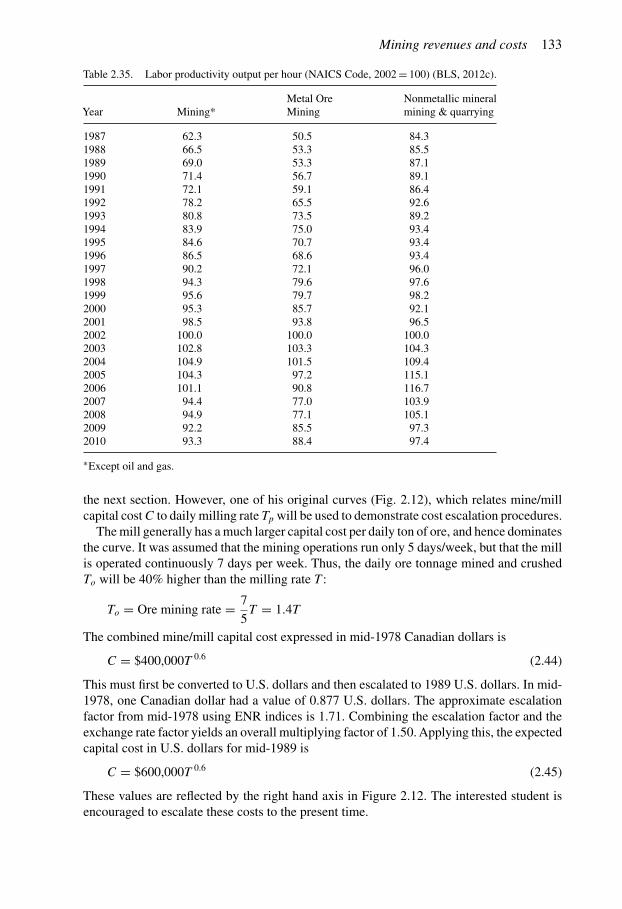
Mining revenues and costs 133
Table 2.35. Labor productivity output per hour (NAICS Code, 2002= 100) (BLS, 2012c).
Metal Ore Nonmetallic mineralYear Mining* Mining mining & quarrying
1987 62.3 50.5 84.31988 66.5 53.3 85.51989 69.0 53.3 87.11990 71.4 56.7 89.11991 72.1 59.1 86.41992 78.2 65.5 92.61993 80.8 73.5 89.21994 83.9 75.0 93.41995 84.6 70.7 93.41996 86.5 68.6 93.41997 90.2 72.1 96.01998 94.3 79.6 97.61999 95.6 79.7 98.22000 95.3 85.7 92.12001 98.5 93.8 96.52002 100.0 100.0 100.02003 102.8 103.3 104.32004 104.9 101.5 109.42005 104.3 97.2 115.12006 101.1 90.8 116.72007 94.4 77.0 103.92008 94.9 77.1 105.12009 92.2 85.5 97.32010 93.3 88.4 97.4
∗Except oil and gas.
the next section. However, one of his original curves (Fig. 2.12), which relates mine/millcapital costC to daily milling rate Tp will be used to demonstrate cost escalation procedures.Themill generally has amuch larger capital cost per daily ton of ore, and hence dominates
the curve. It was assumed that the mining operations run only 5 days/week, but that the millis operated continuously 7 days per week. Thus, the daily ore tonnage mined and crushedTo will be 40% higher than the milling rate T :
To = Ore mining rate = 7
5T = 1.4T
The combined mine/mill capital cost expressed in mid-1978 Canadian dollars is
C = $400,000T 0.6 (2.44)
This must first be converted to U.S. dollars and then escalated to 1989 U.S. dollars. In mid-1978, one Canadian dollar had a value of 0.877 U.S. dollars. The approximate escalationfactor from mid-1978 using ENR indices is 1.71. Combining the escalation factor and theexchange rate factor yields an overall multiplying factor of 1.50.Applying this, the expectedcapital cost in U.S. dollars for mid-1989 is
C = $600,000T 0.6 (2.45)
These values are reflected by the right hand axis in Figure 2.12. The interested student isencouraged to escalate these costs to the present time.

134 Open pit mine planning and design: Fundamentals
Figure 2.12. Mine/mill project capital cost as a function of milling rate (O’Hara, 1980).
2.4.5 The updated O’Hara cost estimator
IntroductionIncluded in the 2nd edition of the SME Mining Engineers Handbook (Hartman, 1992),is an updated chapter on ‘Costs & Cost Estimation’, prepared by O’Hara and Suboleski(1992). They cover the costs associated with both open pit and underground mining. Thissection presents material extracted from their paper. The presentation, however, is organizedsomewhat differently from theirs. All of the costs are expressed in U.S. dollars appropriatefor the third quarter of 1988.Pits may vary greatly in shape, size, and pit slope, especially in mountainous areas or
where the ore and/or waste rock varies greatly in competence. The typical open pit minein North America produces about 43,000 tpd (39 kt/day) of ore and waste from a pit depthof about 400 to 500 ft (120 to 150m), with an oval shaped periphery 2200 ft (670m) wideand 4700 ft (1430m) long. Pit benches are typically 40 ft (12m) high, and overall pit slope(excluding roads) is about 57◦ in pits with competent rock, and 44◦ in pits with oxidized oraltered rock, with in-pit haulage road gradients averaging 9%.The formulas given for equipment sizing, preproduction stripping, and maintenance
facilities presume that the shape and type of open pit is similar, except in daily tonnage, tothe ‘typical’ open pit.
Daily tonnagethe most important factor affecting costs is the size of the mine, primary crusher, andprocessing plant as expressed in terms of the tons of material handled per day of operation.To simplify the discussion the following terms will be introduced:
T = tons of ore milled/dayTo = tons of ore mined/dayTw = tons of waste mined/dayTc = tons of ore passing the primary crusher/dayTp = To + Tw = total material mined/day

Mining revenues and costs 135
In this estimator it is assumed that the mill operates three 8-hour shifts per day and7 days/week irregardless of the shifts worked by the open pit. Many open pit mines oper-ate 7 days/week, but others may operate only 5. In the case of a 5 day/week miningoperation.
T = 5
7To = 0.71To (2.46)
The cost guides in this section are based upon this assumption that the mill capacity is 71%of the daily mined ore tonnage.The crushing plant may operate 5, 6, or 7 days/week, depending on the mine schedule
and whether or not there is adequate fine ore storage capacity to keep the mill supplied withore when the crusher is shut down for repairs or regular maintenance.It is assumed that the crushing plant has the same daily capacity as the mine, but will
work 6 days/week to ensure that the mill will be supplied with crushed ore if the fine orebins have insufficient capacity to keep the mill supplied with ore during the two-day mineshutdown.
Personnel numbersIt may seem somewhat unusual to begin the cost discussion with personnel, but their pro-ductivity is extremely important to the profitability of an operation and their compensationis a major cost item.The number of mine personnel Nop required in open pit mines using shovels and trucks
for loading and hauling the ore may be estimated from the following formulas:
Nop ={0.034T 0.8
p for hard rock
0.024T 0.8p for competent soft rock
(2.47)
The number personnel Nml required to operate mills treating T tons of low-grade ore maybe estimated from the following formulas:
Nml =
⎧⎪⎨⎪⎩5.90T 0.3 for cyanidation of precious metal ores
5.70T 0.3 for flotation of low-grade base metal ores
7.20T 0.3 for gravity concentration of iron ores
(2.48)
The mill crew size (which includes those involved in crushing and/or grinding as well asbeneficiation) as a function of process type and mill rate is shown in Figure 2.13.The number of service personnel Nsv required for open pits mining low grade ore may be
estimated as a percentage of the total mine and mill personnel as shown below:
Nsv = 25.4% of (Nop + Nml) (2.49)
The number of administrative and technical personnel Nat required for a mining and millingplantmay be estimated as a percentage of the total required formining, milling, and services:
Nat = 11% of (Nop + Nml + Nsv) (2.50)
It should be noted that the formulas do not include the personnel required for smelters,refineries, mine townsite services, concentrate transport, or offsite head offices, since theseservices may not be required for many mine projects. Whenever these services can be

136 Open pit mine planning and design: Fundamentals
Figure 2.13. Mill crew size versus mill process and size (O’Hara & Suboleski, 1992).
financially justified for the mine project circumstances, the additional personnel should beestimated separately.
Mine associated capital costsMine site clearing. Prior to beginning construction, the mine/mill site must be first clearedof trees, plants and topsoil. The soil overburden should be stripped to the limits of theultimate pit and stockpiled.The average soil thickness can be found from drilling logs or ultrasonic techniques. By
multiplying the average thickness times the pit area, the volume is determined. As an aidto tonnage calculations, an acre of moist soil averaging 10 ft in thickness contains about23,000 tons of material. For the pit, the required area Ap in acres is
Ap = 0.0173T 0.9p (2.51)
The clearing costs depend upon the topography, the type of cover, and the total area. Theyare expressed as
Total clearing cost =
⎧⎪⎨⎪⎩$1600A0.9
p for 20% slopes with light tree growth
$300A0.9p for flat land with shrubs and no trees
$2000A0.9p for 30% slopes with heavy trees
(2.52)
Clearing, initial stripping and access road costs are plotted as a function of Tp inFigure 2.14.

Mining revenues and costs 137
Figure 2.14. Clearing, stripping and road costs for open pit mines (O’Hara & Suboleski, 1992).
Pre-production waste stripping. The rock overburden above the ore must be stripped toexpose a sufficient amount of ore to supply the planned daily ore tonnage for a period offour to six months. If insufficient ore has been exposed by the pre-production stripping ofwaste, it may become difficult to continue ore mining due to the close proximity of wastebenches where blasting, loading, and haulage of waste is taking place.The location and required area of the ore exposure is determined from ore body mapping.
Once this has been done, the average thickness and area of the waste rock overlying thisore can be computed. Each acre of waste rock averaging 10 ft in thickness contains about40,000 tons of waste.Because of the inverted conical shape of the ultimate open pit, the waste/ore tonnage
ratio at each horizontal bench decreases with each lower bench. Typically, the uppermostore bench to be exposed has a waste/ore ratio of at least twice the waste/ore ratio of theultimate pit. If Ts is the tons of soil, and Tws is the tons of waste rock that must be strippedto expose an amount of ore to sustain four to six months ore production, then the estimatedcosts of waste stripping will be
Soil stripping costs = $3.20T 0.8s for soil not more than 20 ft deep (2.53a)
Waste stripping costs = $340T 0.6ws for rock requiring blasting,
loading, and haulage (2.53b)
Mine equipment(a) Drills. The size, hole diameter, and number of drills required depends on the tons of oreand waste to be drilled off daily.

138 Open pit mine planning and design: Fundamentals
Typically, drill hole sizes have standard diameters of 4, 5, 6(1/2), 7(7/8), 9, 9(7/8), 10(5/8),12(1/4), 13(3/3), 15, and 17(1/2) inches (or 102, 125, 165, 200, 229, 250, 270, 310, 350, 380,and 445 mm). Thus drill selection will be limited to one of these sizes.The tons of ore or waste that are drilled off per day by a drill with a hole diameter of d
inches is:
tons of medium drillable rock = 170d2
tons of easily drillable rock = 230d2 (2.54)
tons of hard drillable rock = 100d2
For the rock defined as ‘medium’ drillable, the expected production rate is about 500 ft pershift.The number of drills Nd should never be less than two. For tonnages up to 25,000 tpd,
two drills of appropriate hole diameter should be chosen. Three drills should be adequatefor up to 60,000 tpd and four or more drills will be required for daily tonnages over 60,000.The cost of the drilling equipment is given by:
Drilling equipment costs = Nd × $20,000d1.8 (2.55)
This formula includes a 25% allowance for drilling and blasting supplies and accessoryequipment.
(b) Shovels. The optimum shovel size S expressed in cubic yards of nominal dipper capacityin relation to daily tonnage of ore and waste Tp to be loaded daily is
S = 0.145T 0.4p (2.56)
The number of shovels Ns with dipper size S that will be required to load a total of Tp tonsof ore and waste daily will be
Ns = 0.011T 0.8p
S(2.57)
In practice, the size of shovel chosen will be one with a standard dipper size close to the sizecalculated by Equation (2.56). The calculated number of shovels Ns usually is not a wholenumber. It should be rounded down. The omitted fractional number expresses the need foreither a smaller-sized shovel or a front-end loader for supplemental loading service. Thissmaller shovel or front end loader must, of course, be capable of loading trucks of a sizeappropriate to the shovels with dipper size S.The total costs of the fleet of shovels supplemented by auxiliary bulldozers and front end
loaders will be
Loading equipment cost = Ns × $510,000S0.8 (2.58)
(c) Trucks. The optimum truck size t in tons that is well matched with shovels of bucketsize S (cubic yards) is
Truck size t (tons) = 9.0S1.1 (2.59)
The total number of trucks Nt of t tons capacity required for the open pit truck fleet, plus anallowance for trucks under repair, is approximated by the following formula:
Nt (Number of trucks required) = 0.25T 0.8p
t(2.60)

Mining revenues and costs 139
Figure 2.15. Costs for open pit equipment (O’Hara & Suboleski, 1992).
The formula for Nt determines the size of the truck fleet under the typical conditionswhere the average haulage distance and gradient outside the pit periphery is less than thehaulage distance and gradient inside the pit periphery. If the waste dump and the ore dumpby the primary crusher are well removed from the pit boundaries, or if the haulage roadbeyond the pit has a steep gradient, it may be necessary to increase the truck fleet size toallow for the longer trip time per load.The cost of haulage equipment including the accessory road maintenance equipment is
given by:
Haulage equipment cost = Nt × $20,000t0.9 (2.61)
The capital costs for the production fleet are given in Figure 2.15.
Pit services(a) Maintenance facilities. The size of maintenance facilities for repair and maintenanceof open pit equipment depends primarily on the number and size of the mine haulagetrucks, which in turn depends on the daily tonnage of ore and waste to be hauled. Repair andmaintenance of the shovels and drills is normally performedon site bymobile repair vehicles.The area in square feet required by the open pit maintenance shop (which should be
located close to the open pit) is as follows:
Area of open pit repair shot = 360T 0.4p (2.62)
Thus the areas of repair shops required for open pit mines are:
Mine size, tpd 10,000 20,000 40,000 80,000Repair shop area, ft2 14,300 18,900 25,000 33,000
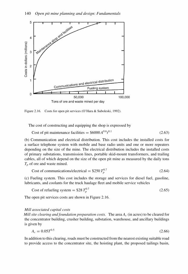
140 Open pit mine planning and design: Fundamentals
Figure 2.16. Costs for open pit services (O’Hara & Suboleski, 1992).
The cost of constructing and equipping the shop is expressed by
Cost of pit maintenance facilities = $6000A0.6t0.1 (2.63)
(b) Communication and electrical distribution. This cost includes the installed costs fora surface telephone system with mobile and base radio units and one or more repeatersdepending on the size of the mine. The electrical distribution includes the installed costsof primary substations, transmission lines, portable skid-mount transformers, and trailingcables, all of which depend on the size of the open pit mine as measured by the daily tonsTp of ore and waste mined.
Cost of communications/electrical = $250 T 0.7p (2.64)
(c) Fueling system. This cost includes the storage and services for diesel fuel, gasoline,lubricants, and coolants for the truck haulage fleet and mobile service vehicles
Cost of refueling system = $28 T 0.7p (2.65)
The open pit services costs are shown in Figure 2.16.
Mill associated capital costsMill site clearing and foundation preparation costs. The area Ac (in acres) to be cleared forthe concentrator building, crusher building, substation, warehouse, and ancillary buildingsis given by
Ac = 0.05T 0.5 (2.66)
In addition to this clearing, roads must be constructed from the nearest existing suitable roadto provide access to the concentrator site, the hoisting plant, the proposed tailings basin,

Mining revenues and costs 141
and the source of the water supply. Costs for clearing and access roads for the surface plantare estimated to be:
Clearing costs = $2000A0.9c for lightly treed area with slopes of
not more than 20% gradient(2.67a)
Access roads = $280,000 per mile for 30-ft (9-m) wide graveled road inmildly hilly region
(2.67b)
The formulas should be modified ±30% for more adverse or more favorable slope and treegrowth conditions.Soil overburden must be stripped wherever buildings and facilities are to be sited. The
cost of stripping soil overburden Do feet deep over and area of A acres will be:
Cost of soil stripping = $1000A0.8Do (2.68)
After the soil overburden is removed and the underlying rock or basal strata is exposed, thisrock or strata will require localized removal, probably by drilling and blasting, to establishsound foundation conditions over levelled areas for the plant buildings and plant equipment.If there are Cu cubic yards of rock requiring drilling, blasting, and haulage to a dump site,this mass excavation will cost:
Cost of mass excavation = $200C0.7u (2.69)
for excavations of up to 100,000 yd3.If the mass excavation is in rock that can be broken by ripping, the cost will be only 20%
of that indicated.When the mass excavation has been completed, detailed excavation to tailor the rock
surface to the exact levels for pouring concrete foundations can be done. At the same time,suitable fill will be placed and compacted over level areas where deep trenches of soft soilhave been removed. If there areCd cubic yards of rock to be excavated by detailed excavationand Fc cubic yards of compacted fill to be placed, the cost will be:
Excavated and fill compaction = $850C0.6d + $75F0.7
c (2.70)
Concrete costs for the foundations of the concentrator building, fine ore bins, and concen-trator equipment probably will cost between $350 and $900/yd3, depending on whether theconcrete pour is for a simple form with little reinforcing steel or for a complex form that isheavily reinforced. The concrete cost may be significantly higher per cubic yard if concreteis scheduled to be poured in winter months when the temperature is below 40◦F (4.4◦C) andheating of aggregate and water and heating of concrete forms is required for sound concrete.It is difficult to estimate the shape and volume of concrete forms before these forms
have been designed, and hence concrete costs related to concrete volume are unreliable forpreliminary estimation. Assuming no difficulties
Approximate concrete foundation costs = $30,000 T 0.5 (2.71)
These different costs are shown in Figure 2.17 as a function of daily plant capacity.
Concentrator building. The costs of the concentrator building include all costs of construct-ing the building above the concrete foundations and enclosing the building, plus the costof internal offices, laboratories, and changerooms. It does not include the cost of process

142 Open pit mine planning and design: Fundamentals
Figure 2.17. Costs for surface plant clearing, excavation and foundations (O’Hara & Suboleski, 1992).
equipment, piping, or electrical wiring, because these items are included in the costs of eachfunctional area. The equipment in operating concentrators generates a substantial amountof heat and comfortable working conditions can be attained with little or no insulation, aslong as the concentrator is located in a region with a mild climate. For flotation mills locatedin a mild climate
Cost of building = $27,000 T 0.6 (2.72)
A ‘mild climate’ is defined as a region where the degree-days are about 7000 (in ◦F) or 4000(in ◦C) per year. Weather stations usually record the ‘degree-days’ (◦F × D, or ◦C × D),which represents the average number of days times the degrees that the temperature isbelow 65◦F or 18◦C. In hot climates, where freezing temperatures are not experienced,the building costs may be reduced by only partially enclosing the building and by locatingthickeners and other hydrometallurgical equipment outside the building. In cold climates,the additional cost of insulation, heating, and snow loading is likely to increase the build-ing cost by about 10% for each increase of 1800 (◦F × D) above 7000 or 1000 (◦C × D)above 4000.
Primary crushing plant with gyratory crusher. Open pit mines generally place the primarycrusher on the surface outside the pit, within convenient conveying distance to the coarseor stockpile and the fine ore crushing plant. Open pit trucks normally dump the ore ontoa grizzly mounted over the gyratory crusher which discharges crushed ore to a conveyor.Because of the headroom required to operate and discharge the crushed ore from a gyratorycrusher, a substantial excavation and volume of concrete is required for the primary crusher

Mining revenues and costs 143
Figure 2.18. Costs for the concentrator building and crushing plant (O’Hara & Suboleski, 1992).
plant. The cost of the primary crusher depends on the size and capacity of the gyratorycrusher selected for crushing Tc tons of ore daily:
Cost of gyratory crusher = $63 T 0.9c (2.73)
The cost of excavating and concreting the foundations for the primary crusher, installingthe crusher, construction of the truck dump and grizzly, plus the coarse ore conveyor andfeeder under the crusher is:
Cost of primary crushing plant = $15,000 T 0.7c (2.74)
The cost of the crusher itself is not included.
Fine ore crushing and conveyors. This cost includes the crushing plant building, installedequipment and conveyors.
Cost of fine ore crushing plant = $18,000 T 0.7 (2.75)
Note: The cost may be 12% higher if the conveyors must be enclosed and heated.
Grinding section and fine ore storage. Thefine storage binsmust have sufficient live capacityto provide mill feed for at least the number of days that the crushing plant is idle per week.The cost of the fine ore bins will be proportional to the weight of steel used in constructingthese bins, and the weight of steel will be proportional to T 0.7.The size and cost of the grinding mills depend on the tons of ore to be ground daily by
each mill, but they also depend on the hardness of the ore as measured by the work index

144 Open pit mine planning and design: Fundamentals
Figure 2.19. Costs for the grinding section, storage bins and tailings storage (O’Hara & Suboleski, 1992).
and the fineness of grind that is required to attain the desired concentration and recovery ofvaluable minerals.
Cost of grinding and bins =
⎧⎪⎪⎪⎪⎪⎪⎪⎪⎪⎪⎪⎨⎪⎪⎪⎪⎪⎪⎪⎪⎪⎪⎪⎩
$18,700 T 0.7 for medium hard orewith a work index of 15, groundto 70% passing 200 mesh
$12,500 T 0.7 for soft ores groundto 55% passing 200 mesh
$22,500 T 0.7 for hard ores with awork index of higher than 17, groundto 85% passing 200 mesh
(2.76)
These costs are plotted in Figure 2.19 as a function of plant capacity.
Processing and related sections. The capital costs in this section cover the purchase andinstallation of all equipment required to concentrate or extract valuable minerals from theslurried ground ore, and process the concentrates or extracted minerals into dried solidsor impure metals that are directly salable as dry concentrates, ingots of precious metals,uranium yellowcake, or impure metallic gravity concentrates of alloy metals. These capitalcosts include equipment and tanks for thickening, filtering, precipitation, leaching, solventextraction, etc., plus all process piping, electrical wiring, and process control.Process costs for different types of ore by different methods are listed below:
1. High-grade gold ores leached by cyanidation, followed by zinc dust precipitation of goldby Merrill Crowe process, filtering, drying, and gold refining:
Process capital costs = $60,200 T 0.5 (2.77)

Mining revenues and costs 145
2. Low-grade ores, cyanide leaching, CIP (carbon-in-pulp) or CIL (carbon-in-leach)adsorption, refining:
Process capital costs = $47,300 T 0.5 (2.78)
3. High-grade gold ores with base metal sulfides; cyanide leaching, secondary flotation,carbon adsorption by CIP or CIL process, filtering, thickening, drying, and refining:
Process capital costs = $103,200 T 0.5 (2.79)
4. Simple low-grade base metal ores of copper with minor content of gold, which can berecovered as smelter credits. Flotation, thickening, filtering, and drying of auriferous copperconcentrates:
Process capital costs = $13,700 T 0.6 (2.80)
5. Pyritic gold/silver ores where the precious metals are locked in the pyritic minerals.Differential flotation, selective roasting, recovery of deleterious materials, cyanidation,thickening, precipitation, filtering, and refining.
Process capital costs = $180,000 T 0.5 (2.81)
6. High-grade Cu/Pb ores, Cu/Zn ores, Pb/Zn ores, Cu/Ni ores. Recovery by differentialflotation, thickening, filtering, and drying of separate concentrates:
Process capital costs = $20,600 T 0.6 (2.82)
7. Complexbasemetal ores containing at least three valuablemetals, with recoverableminoramounts of precious metals; Cu/Zn/Pb ores, Pb/Zn/Ag ores, Cu/Pb/Ag ores, Cu/Zn/Auores. Recovery by differential flotation, separate thickening, filtering, and drying of severalconcentrates and/or bulk concentrates.
Process capital costs = $30,100 T 0.6 (2.83)
8. Non-sulfide ores containing specialty metals such as columbium (niobium), tantalum,tungsten, and tin in minerals that do not respond to flotation, and which are separated byspecialized gravity concentration methods:
Process capital costs = $5000 T 0.7 to $13,000 T 0.7 (2.84)
9. Uranium ores: acid leaching, countercurrent decantation, clarification, solvent extractionand yellowcake precipitation:
Process capital costs = $150,000 T 0.5 to $200,000 T 0.5 (2.85)
Figure 2.20 is a plot of these relationships.
Initial tailings storage. There are many aspects of tailings storage such as topography, dis-tance frommill to tailings site, localized environmental concerns, etc., that could drasticallyalter the costs of tailings storage. If, however, all adverse aspects are absent, and a suitabletailings site is available within two miles of the mill, and the nature of the tailings does nothave adverse environmental effects, the minimum cost of tailings storage may be:
Minimum tailings storage cost = $20,000 T 0.5 (2.86)
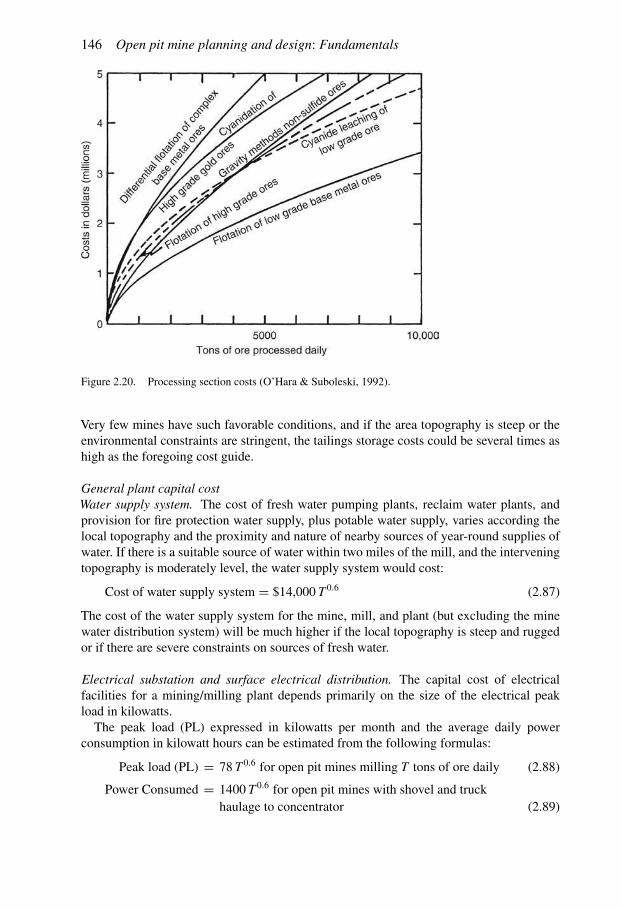
146 Open pit mine planning and design: Fundamentals
Figure 2.20. Processing section costs (O’Hara & Suboleski, 1992).
Very few mines have such favorable conditions, and if the area topography is steep or theenvironmental constraints are stringent, the tailings storage costs could be several times ashigh as the foregoing cost guide.
General plant capital costWater supply system. The cost of fresh water pumping plants, reclaim water plants, andprovision for fire protection water supply, plus potable water supply, varies according thelocal topography and the proximity and nature of nearby sources of year-round supplies ofwater. If there is a suitable source of water within two miles of the mill, and the interveningtopography is moderately level, the water supply system would cost:
Cost of water supply system = $14,000 T 0.6 (2.87)
The cost of the water supply system for the mine, mill, and plant (but excluding the minewater distribution system) will be much higher if the local topography is steep and ruggedor if there are severe constraints on sources of fresh water.
Electrical substation and surface electrical distribution. The capital cost of electricalfacilities for a mining/milling plant depends primarily on the size of the electrical peakload in kilowatts.The peak load (PL) expressed in kilowatts per month and the average daily power
consumption in kilowatt hours can be estimated from the following formulas:
Peak load (PL) = 78 T 0.6 for open pit mines milling T tons of ore daily (2.88)
Power Consumed = 1400 T 0.6 for open pit mines with shovel and truckhaulage to concentrator (2.89)

Mining revenues and costs 147
Typically, the concentrator and related facilities account for about 85% of the total powerconsumption for open pit mines and concentrators.The cost of power supply depends on whether the power is generated by an existing
electric utility or by a mine diesel-electric plant. Small mines in remote areas may be forcedto generate their own electric power, because the cost of a lengthy transmission line from anexisting utility may be too high due to the low peak load and low electric power consumptionof a small mine.If the mine is supplied with utility power, the cost of a utility substation with step-down
transformers will be
Cost of substation = $580(PL)0.8 (2.90)
The cost of installing low-voltage power distribution to the surface concentrator, crushingplant, and surface facilities, but excluding the distribution to the surface open pit is likelyto be
Cost of surface power distribution = $1150(PL)0.8 (2.91)
A diesel-electric generating plant may be required for a small mine in a remote area or by alarger mine supplied with utility power that may require a standby electric power plant forprotection of vital equipment.
Cost of diesel-electric plant = $6000(PL)0.8 (2.92)
General plant services. These costs include the costs of constructing, furnishing, and equip-ping the general administrative office, general warehouse, electrical and mechanical repairshop (for smaller mill equipment and services equipment), vehicle garages, changehouses,first aid and mine rescue stations, security stations plus general purpose vehicles, parkinglots, and yard fencing.The size of the buildings tends to depend on the number of employees served by each
building. It is necessary to estimate the building size in square feet before estimating buildingcost, which will vary with the area of each type of building.
(a) Administrative office. The floor space per person tends to increase as the number ofadministrative and technical staffNat becomes larger. This reflects themore complex recordsof accounting and technical staff and the consequent requirement ofmore space for computerfacilities, mining plans, and reference file facilities.
A = Office are required in ft2 = 35N1.3at
Cost of office = $155A0.9 (2.93)
(b) Maintenance shop. Maintenance personnel Nsv will require about 85 ft2/person formaintenance and repair of movable equipment from the mill and service departments.
Cost of shop = $102(85Nsν)0.9 (2.94)
(c) Mine changehouse. The mine changehouse requires about 24 ft2/person on the minepayroll and includes the first aid station and mine rescue facilities.
Changehouse cost = $125(24Nop)0.9 (2.95)

148 Open pit mine planning and design: Fundamentals
Figure 2.21. Costs of plant service facilities (O’Hara & Suboleski, 1992).
(d) Surface warehouse. This should accommodate all supplies and spare parts for the mine,mill, and service facilities that must be kept indoors. Bulky supplies such as rough lumber,structural steel, etc., can be stored outdoors in most climates.
Surface warehouse cost = $5,750 T 0.4 (2.96)
(e) Miscellaneous surface facilities. This includes general purpose vehicles and garages,security stations and fencing, parking lots, and miscellaneous services.
Miscellaneous surface facilities = $10,000 T 0.5 (2.97)
Those general plant capital costs dependent on plant capacity are shown in Figure 2.21.
Mine project overhead costsIn addition to the direct costs for specific facilities for a mine project, which may total manymillions of dollars, there are substantial costs and expenses involved in project design,general site costs, supervision and administration, and provision of working capital. Theseoverhead costs may be estimated as a function of the total direct costs D in dollars.
Engineering. This includes the costs of feasibility studies, environmental impact studies,design engineering, equipment specifications and procurement, and specialized consultingservices:
Engineering costs = $2.30D0.8 (2.98)
General site costs. This includes construction camp costs, specialized constructionequipment, and general construction site costs:
General site costs = $0.310D0.9 (2.99)

Mining revenues and costs 149
Project supervision. This includes project supervision, scheduling and budgeting, andconstruction management:
Project supervision costs = $1.80D0.8 (2.100)
Administration. This includes local office administration by corporate owner’s represen-tatives, accounting and payment of general contractor, legal costs, plus preproductionemployment of key operating staff:
Administration costs = $1.50D0.8 (2.101)
Project overhead costs as a percentage of direct project costs tend to vary depending on thesize and complexity of the project. The lower percentages of 4 to 6% would be typical for$100 million projects and conventional technology, whereas the higher percentages of 8 to11% would apply to smaller $10 million project that are technically novel or complex.
Working capital. The allowance for working capital for a mining project should be sufficientto cover all operating costs plus purchase of the initial inventory of capital spares and partsuntil revenue is received from smelters or purchasers of metallic products. The time periodelapsing before receipt of revenue sufficient to pay imminent operating costs will varydepending on the smelter terms or marketing terms, but the typical allowance is about 10weeks after the concentrator is operating at full capacity.Typical working capital allowance is equal to the operating costs for 10 weeks after
commissioning of concentrator plus cost of purchasing initial inventory of capital sparesand parts.Whenever the mine or mill design is based on extensive usage of reconditioned used
equipment, there is a higher frequency of equipment downtime that requires additional timeallowance of working capital; this will decrease the apparent savings of used equipment.The total overhead costs as a summation of the different components are shown in
Figure 2.22.
Figure 2.22. Project overhead versus direct costs (O’Hara & Suboleski, 1992).

150 Open pit mine planning and design: Fundamentals
Daily operating costsIntroduction. In this section the operating costs per day for each activity will be presentedin the form
Operating cost = KTxI (2.102)
The operating cost per ton can be derived from the given formula simply by dividing theoperating cost per day by the tons mined (or processed) per day. If, for example,
Operating cost per day = 100 T 0.7I (2.103)
the operating cost per ton is
Operating cost per ton = 100T 0.7I
TI= 100 T 20.3
I (2.104)
Pit operating costs. The operating costs of open pit mines depends on the size and numbersof drills, shovels, and trucks, which in turn is dependent on the tons per day of ore andwaste. In most open pit mines mining low grade ore, there is little if any difference in thespecific gravities, blasting characteristics, and drillabilities of ore or waste, and the haulagedistance to the ore dump usually does not differ very much from the waste haulage distance.Consequently, the cost of mining a ton of ore will be virtually the same as the cost of mininga ton of waste.The daily operating costs are:
Drilling cost per day = $1.90 T 0.7p (2.105)
Blasting cost per day = $3.17 T 0.7p (2.106)
Loading cost per day = $2.67 T 0.7p (2.107)
Haulage cost per day = $18.07 T 0.7p (2.108)
General services cost per day = $6.65 T 0.7p (2.109)
The open pit general services cost includes the cost of pit maintenance, road grading, wastedump grading, pumping, and open pit supervision, but it does not include the cost of primarycrushing or electric power.
Concentrator operating costs. Although the gyratory crusher may be located at the edge ofthe open pit, the costs of operating it are grouped under milling costs (rather than as openpit operating costs) since it is the first stage of ore treatment.The design of the milling flowsheet is usually optimized after extensive testwork on the
types of processes tailored to the characteristics of the ore. At the preliminary feasibilitystage however, the optimum processing requirements are not known with accuracy, and thecosts of processing can only be approximately estimated.The following cost guides are offered as rough estimates of crushing and concentrating
costs per day.
(a) Primary crushing. This cost includes the cost of primary crushing, the cost of conveyingthe primary crushed ore to the coarse ore stockpile, plus operating costs of the coarse orestockpile.
Crushing costs per day = $7.90 T 0.6 (2.110)

Mining revenues and costs 151
(b) Fine crushing and conveying. This includes fine crushing, conveying from coarse orestorage, and conveying to the fine ore bins.
Fine crushing costs per day = $12.60 T 0.6 (2.111)
(c) Grinding. This cost includes the fine ore bin storage and the rod mills, ball mills, and/orSAG (semiautogenous grinding) mills:
Grinding section costs per day = $4.90 T 0.8 (2.112)
(d) Process section. This includes the operating costs of all sections that involve concentra-tion of ore by flotation or by gravity, leaching of metals from ore, thickening of slurries,ion exchange, precipitation, filtering, drying, and recovery of metallic concentrations, ordeleterious materials that would otherwise penalize smelter revenue.
Processing costs =
⎧⎪⎪⎪⎪⎪⎪⎪⎪⎪⎪⎪⎪⎪⎪⎪⎪⎨⎪⎪⎪⎪⎪⎪⎪⎪⎪⎪⎪⎪⎪⎪⎪⎪⎩
$65 T 0.6 for cyanidation of gold/silver ores (2.113a)
$54 T 0.6 for flotation of simple base (2.113b)metal ores
$34 to $41 T 0.7for complex base metalores varying in complexity (2.113c)
$65 T 0.7 for uranium ores by leaching,CCD, solvent extraction, and precipitation (2.113d)
$45 T 0.7 for nonfloatable nonsulfide oresreponding to gravity separation (2.113e)
per day
Tailings costs per day = $0.92 T 0.8 for all concentrators (2.113f)
Assaying costs per day = $1.27 T 0.8 for all concentrators (2.113g)
Supervision, maintanance, = $40.80 T 0.8 for all concentratorsand general costs per day (2.113h)
Processing costs would be decreased to 55% of those shown by the foregoing formulaswhen low-grade ore, typically mined by open pit mining, is being treated by a concentratorthat rejects tailings at an early stage.
Other operating costs(a) Electrical power. Expressions for the peak load and daily power requirements for theopen pit, crushing plant and concentrator, etc. have been given earlier. The power cost foropen pit mines and plants processing T tons of ore per day is
Cost of electric power = $145 T 0.56 (2.114)
(b) Surface services. The daily cost of each person in the surface maintenance and generalservices departments is estimated to be $141 in wages and fringe benefits, plus an averagecost of $16 in supplies consumed. If the number of maintenance and general servicespersonnel is Nsv, then the daily costs of maintenance and general services departments is
Services cost per day = $157Nsv (2.115)

152 Open pit mine planning and design: Fundamentals
The daily costs of the administrative and technical staff, including supplies and ser-vices required by them, plus fixed costs for local property taxes and legal fees paid byadministrative services, are proportional to the number of staff Nat .
Each staff person is estimated to cost on the average $185 in salary per day, and toconsume $37.60 in supplies and services per day.
Total cost per day for administrative and = $222.60Nat
technical staff salaries and supplies (2.116)
(c) Additional assistance in cost estimation. O’Hara and Suboleski (1992) suggest that thefollowing sources/publications may be of assistance to those making cost estimates.1. General Construction Estimation Standards, 6 volumes, revised annually, published
by Richardson Engineering Services, Inc., P.O. Box 1055, San Marcos, CA 92069.2. Means Construction Costs, revised annually, and published by Robert Snow Means
Co., Inc., 100 Construction P1., Kingston, MA 02364.3. US Bureau of Mines Cost Estimating System Handbook, 2 volumes, Information Cir-
cular 9142 (surface and underground mining), and Information Circular 9143 (mineralprocessing). Mining and milling costs are as of January 1984. The two volumes, IC 9143,are available from the Superintendent of Documents, U.S. Government Printing Office,Washington, DC 20402.
4. Canadian Construction Costs: Yardsticks for Costing, revised annually; available fromSoutham Business Publications, 1450 Don Mills Rd., Don Mills, ON, Canada, M3B 2X7.5. Mining and Mineral Processing Equipment Costs and Preliminary Capital Cost
Estimations, Special Vol. 25, 1982; published by The Canadian Institute of Mining andMetallurgy, 1 Place Alexis Nihon, 1210-3400 de Maisonneuve Blvd. W., Montreal, PQ,Canada H3Z 3B8.A recent addition to this list of useful publications is "CAPCOSTS: A Handbook for
Estimating Mining and Mineral Processing Equipment Costs and Capital Expenditures andAiding Mineral Project Evaluations" byAndrew L. Mular and Richard Powlin. Special Vol.47, 1998; published by The Canadian Institute ofMining, Metallurgy and Petroleum, XeroxTower, 1210-3400 de Maisonneure Blud. W., Montreal, PQ, Canada H3Z 3B8. Since thepassing of T. A. O’Hara, no one, unfortunately, has continued to update his useful curves.
2.4.6 Detailed cost calculations
Before discussing some techniques for estimating mining costs, a more detailed costexamination will be presented. With this as a basis, the costs will be grouped in severalways to show the dependence on accounting practice. The overall process is as follows:
Step 1. Given the annual production requirements for ore and waste plus the operatingschedule, determine the daily production rate.
Step 2. Select a basic equipment fleet.
Step 3. Calculate the expected production rate for each type of equipment. Calculate thenumber of machines required. Determine the amount of support equipment needed.
Step 4. Determine the number of production employees required. Determine the number ofsupport employees.
Step 5. Calculate the owning and operating costs for the equipment.

Mining revenues and costs 153
Step 6. Calculate the other costs.
Step 7. Calculate the overall cost per ton.
This procedure will be demonstrated using an example presented by Cherrier (1968).Although the costs are old, the process remains the same.
The cross-sections through the molybdenum orebody used in this example will bepresented in Chapter 3. The initial mine design has indicated a pit for which
– Rock type is granite porphyry,– 32,300,000 tons of waste,– 53,000,000 tons of ore,– Stripping ratio SR equals 0.6:1, and– Average ore grade is 0.28% MoS2.
The waste will be hauled by trucks to a dump area. The ore will be hauled by trucks to oneof two ore passes. The ore is crushed and then transported by underground conveyor to themill. The step-by-step process will be developed.
Step 1: Daily production rate determination. It has been decided that the annual productionrate will be
– 3,000,000 tons ore and– 2,000,000 tons waste.
The mine will operate 2 shifts/day, 5 days/week, 52 weeks per year, with 10 holidays.The ore and waste production per shift becomes:– Ore: 6000 tons/shift,– Waste: 4000 tons/shift.
Step 2: Selection of a consistent set of pit equipment. The major types of productionequipment to be selected are:
– Drills,– Shovels,– Trucks.The bench height has been chosen to be 30 ft. The basic equipment fleet selected
consists of:– 6 yd3 electric shovels,– 35 ton capacity rear dump trucks,– Rotary drills capable of drilling 9 7/8
′′ diameter hole.
Step 3: Production capacity/Number of machines. Based upon a detailed examination ofeach unit operation, the following production rates were determined:
– Drills: 35 ft of hole per hour,– Shovels (waste): 630 tons/hour,– Shovels (ore): 750 tons/hour,– Trucks (waste): 175 tons/hour,– Trucks (ore): 280 tons/hour.
From this, of the number production units and required scheduling were determined for oreand waste:
– Ore1 drill (1 shift/day),1 shovel (2 shifts/day),3 trucks (2 shifts/day).

154 Open pit mine planning and design: Fundamentals
– Waste1 drill (1 shift/day),1 shovel (2 shifts/day),4 trucks (2 shifts/day).
The support equipment includes:– 4 dozers (2 shifts/day),– 2–5 yd3 rubber tired front end loaders (2 shifts/day),– 2 road graders (2 shifts/day),– 1 water truck (2 shifts/day),– 1 explosives truck (1 shift/day).
The reserve production equipment to be purchased is:– 2–35 ton trucks,– 1–5 yd3 front end loader.In case of shovel breakdown, a front end loader will substitute.
Step 4: Determine the number of production employees. A manpower scheduling chart isprepared such as is shown in Table 2.36. The overall numbers are summarized below.
– 1 assistant superintendent,– 4 shift foreman,– 4 shovel operators,– 4 oilers,– 14 truck drivers,– 2 drillers,– 2 driller helpers,– 1 blaster,– 1 blaster helper,– 8 dozer operators,– 4 loader operators,– 4 grader operators,– 2 water truck drivers,– 4 truck spotters,– 4 crusher operators,– 4 conveyor operators,– 10 laborers.
As can be seen, there are 73 production employees.The crusher/conveyor part of the production system operates 7 days/week and 3 shifts per
day. There is one crusher operator and one conveyor operator per shift. The ore passes containenough storage capacity so that the mill can run 7 days/week even though the mine runs 5.
Step 5: Determine the number of other employees. There are four basic departments at themine:
– Administration,– Engineering,– Mine,– Maintenance.The overall structure is shown in Figure 2.23. The administration and engineering
departments work straight day shift. The maintenance department works two shifts/day,5 days per week as shown in the manpower chart (Table 2.37).

Mining revenues and costs 155
Table 2.36. Production employees manpower estimate.
(a) Salaried manpower estimate
Classification Shift requirements Manshifts per No. ofweek req’d
Sun. Mon. Tue. Wed. Thur. Fri. Sat. men
A B C A B C A B C A B C A B C A B C A B C A B C Total
Assist. supt. 1 1 1 1 1 5 5 1Shift 2 2 2 2 2 10foreman 2 2 2 2 2 10 20 4
Total 5
(b) Day pay manpower estimate
Classification Shift requirements Manshifts per No. ofweek req’d
Sun. Mon. Tue. Wed. Thur. Fri. Sat. men
A B C A B C A B C A B C A B C A B C A B C A B C Total
Shovel 2 2 2 2 2 10operator 2 2 2 2 2 10 20 4
Shovel 2 2 2 2 2 10oiler 2 2 2 2 2 10 20 4
Truck 7 7 7 7 7 35driver 7 7 7 7 7 35 70 14
Doser 4 4 4 4 4 20operator 4 4 4 4 4 20 40 8
Drill 2 2 2 2 2 10 10 2operator
Drill 2 2 2 2 2 10 10 2helper
Loader 2 2 2 2 2 10operator 2 2 2 2 2 10 20 4
Grader 2 2 2 2 2 10operator 2 2 2 2 2 10 20 4
Water truck 1 1 1 1 1 5driver 1 1 1 1 1 5 10 2
Truck 2 2 2 2 2 10spotters 2 2 2 2 2 10 20 4
Blaster 1 1 1 1 1 5 5 1Blaster 1 1 1 1 1 5 5 1helper
Crusher 1 1 1 1 1 1 1 7operator 1 1 1 1 1 1 1 7
1 1 1 1 1 1 1 7 21 4Conveyer 1 1 1 1 1 1 1 7operator 1 1 1 1 1 1 1 7
1 1 1 1 1 1 1 7 21 4Laborers 5 5 5 5 5 25
5 5 5 5 5 25 50 10
Total 68

156 Open pit mine planning and design: Fundamentals
Figure 2.23. Mine personnel requirements (Cherrier, 1968).
Step 6: Determine the payroll cost. Table 2.38 summarizes the basic annual wage figuresfor the various job classifications. Fringe benefits amounting to 25% are not included in thistable.
Step 7: Determine the operating costs for the equipment. The total operating costs for thevarious unit operations include materials, supplies, power and labor. These are summarizedin Table 2.39. The labor cost includes the 25% fringe benefits.Note that there are three different units which have been used to express the costs ($/ft,
$/hr and $/ton). Some conversion factors are required to obtain the desired common valuesof $/ton. These are:
– Drilling: 27.2 tons/ft,– Loading (ore): 750 tons/hr,– Loading (waste): 630 tons/hr,– Hauling (ore): 750 tons/hr (3 trucks),– Hauling (waste): 630 tons/hr (4 trucks).To simplify the presentation, only two cost categories will be carried further. These are
operating labor and MEP (material, expenses and power) which includes all of the rest. Theore-waste separation will be made. The results are summarized in Tables 2.40 and 2.41.It is noted that the labor cost is strictly for operating labor and does not include repair
labor nor does it include supervision.
Step 8: Determine the capital cost and the ownership cost for the equipment. The capitalcost for the pit equipment is given in Table 2.42.During the life of the mine, some of the equipment will have to be replaced. This is
indicated in Table 2.43. As can be seen, the original equipment falls into three lifetimegroups (5, 10 and 20 years). These are summarized below:
Life (yrs) Total original cost ($)5 861,00010 396,00020 1,401,000

Mining revenues and costs 157
Table 2.37. Maintenance employees manpower estimate.
(a) Salaried manpower estimate
Classification Shift requirements Manshifts per No. ofweek req’d
Sun. Mon. Tue. Wed. Thur. Fri. Sat. men
A B C A B C A B C A B C A B C A B C A B C A B C Total
Shop 1 1 1 1 1 5 5 1foreman
Shift 1 1 1 1 1 5foreman 1 1 1 1 1 5 10 2
Master 1 1 1 1 1 5 5 1mechanic
Total 4
(b) Day pay manpower estimate
Classification Shift requirements Manshifts per No. ofweek req’d
Sun. Mon. Tue. Wed. Thur. Fri. Sat. men
A B C A B C A B C A B C A B C A B C A B C A B C Total
Mechanic 3 3 3 3 3 153 3 3 3 3 15 30 6
Electrician 1 1 1 1 1 51 1 1 1 1 5 10 2
Machinist 1 1 1 1 1 51 1 1 1 1 5 10 2
Greaser 1 1 1 1 1 51 1 1 1 1 5 10 2
Oiler 1 1 1 1 1 51 1 1 1 1 5 10 2
Welder 1 1 1 1 1 51 1 1 1 1 5 10 2
Helper 2 2 2 2 2 102 2 2 2 2 10 20 4
Janitor 1 1 1 1 1 51 1 1 1 1 5 10 2
Total 22
The equipment ownership cost consists of two parts:(1) Depreciation,(2) Average annual investment cost.
Straight line depreciation with zero salvage value is assumed. Thus the average equipmentdepreciation per year is $281,850. The average annual investment (AAI) is calculated usingthe following formula.
AAI = n + 1
2nCC (2.117)
where n is the life (yrs) and CC is the capital cost ($).

158 Open pit mine planning and design: Fundamentals
Table 2.38. Annual payroll (Cherrier, 1968).
Classification Number required Unit annual age Total annual age
AdministrationMine superintendent 1 $25,000 $25,000Office manager 1 13,000 13,000Clerk 1 7,000 7,000Pro-rated G&A personnel(average salary $8,000) 10 8,000 80,000__ ________
Total 13 $125,000
EngineeringChief engineer 1 $16,000 $16,000Mining engineers 2 9,500 19,000Safety engineer 1 8,000 8,000Industrial engineer 1 8,500 8,500Geologist 1 7,500 7,500Surveyors 2 7,500 15,000Surveyor helpers 4 5,500 22,000Draftsmen 3 6,000 18,000Samplers 2 5,500 11,000__ ________
Total 17 $125,000
MineAss’t mine superintendent 1 $18,000 $18,000Shift foreman 2 11,000 22,000Shovel operators 4 8,500 34,000Shovel oilers 4 6,000 24,000Truck drivers 14 7,000 84,000Drillers 3 8,000 24,000Driller helpers 3 6,500 19,500Blaster 1 8,500 8,500Blaster helper 1 6,500 6,500Dozer operators 8 8,000 64,000Loader operators 6 8,000 48,000Grader operators 4 8,000 32,000Water truck driver 2 7,000 14,000Crusher operators 4 7,500 30,000Conveyor operators 4 7,500 30,000Truck spotters 4 5,500 22,000Laborers 10 5,000 50,000__ ________
Total 73 $526,500
MaintenanceShop foreman 1 $14,000 $14,000Shift foreman 2 10,500 21,000Master mechanic 1 11,000 11,000Mechanics 6 8,500 51,000Electricians 2 8,000 16,000Machinist 2 7,000 14,000Greaser 2 6,000 12,000Oiler 2 6,000 12,000Welder 2 6,500 13,000Helpers 4 5,500 22,000Janitor 2 5,000 10,000__ ________
Total 26 $196,000

Mining revenues and costs 159
Table 2.39. Mine operating costs (Cherrier, 1968).
Unit operation Cost category $/ft $/hr $/ton
Drilling Bits 0.100Maintenance, lub, repairs 0.200Supplies 0.015Fuel 0.250Labor 0.133
Blasting Ammonium nitrate 0.0125Fuel oil 0.0010Primers 0.0020Primacord, caps, fuse 0.0030Labor 0.0030
Loading Repairs, maintenance, supplies cost 7.20Power per 1.65Lubrication shovel 0.10Labor 8.75
Hauling Tires cost cost 1.65Tire repairs per 0.25Repairs, maintenance truck 2.70Fuel 0.96Oil, grease 0.40Labor 3.60
Auxilliary Tracked dozer materials 0.015equipment Rubber tired dozer supplies 0.013
Front end loader repairs 0.010Graders fuel 0.020Water truck 0.005Labor 0.040
Secondary drilling MEP 0.005and blasting Labor 0.005
Crushing MEP 0.020Labor 0.010
Conveying MEP 0.018Labor 0.013
Snow removal MEP 0.005Labor 0.005
Table 2.40. Summary of direct operating expenses for ore (Cherrier, 1968).
Unit operation Cost ($/ton) Total
MEP Labor
Drilling 0.021 0.005 0.026Blasting 0.019 0.003 0.022Loading 0.012 0.012 0.024Hauling 0.024 0.014 0.038Auxilliary 0.063 0.040 0.103Secondary D&B 0.005 0.005 0.010Crushing 0.020 0.010 0.030Conveying 0.018 0.013 0.031Snow removal 0.005 0.005 0.010
Total 0.187 0.107 0.294

160 Open pit mine planning and design: Fundamentals
Table 2.41. Summary of direct operating expenses for waste (Cherrier, 1968).
Unit operation Cost ($/ton) Total
MEP Labor
Drilling 0.021 0.005 0.026Blasting 0.019 0.003 0.022Loading 0.014 0.018 0.032Hauling 0.038 0.029 0.067Auxilliary 0.063 0.040 0.103Secondary D&B 0.005 0.005 0.010Snow removal 0.005 0.005 0.010
Total 0.165 0.105 0.270
Table 2.42. Capital costs and annual depreciation for the mining equipment (Cherrier, 1968).
Operation and Item No. Unit cost Total cost Life (yrs) Annual deprec.
DrillingBucyrus Erie 40-RRotary drill 2 $75,000 $150,000 10 $15,000
BlastingPowder truck 1 8,000 8,000 10 800
ExcavatingP&H shovel model 1400 2 288,000 576,000 20 28,800
Haulage and TransporationHaulpak 35 ton trucksrear dump 9 58,000 522,000 5 104,400Crusher 2 150,000 300,000 20 15,000Conveyor 1 395,000 395,000 20 19,750Chloride spray system 2 15,000 30,000 20 1,500
Pit maintenanceBulldozers 3 50,000 150,000 5 30,000Rubber tired dozers 3 40,000 120,000 5 24,000Front end loaders 2 45,000 90,000 10 9,000Road graders 3 25,000 75,000 10 7,500Sprinkler truck 2 7,000 14,000 10 1,400Fuel truck 1 9,000 9,000 10 900Mobile maintenance 1 15,000 15,000 10 1,500
MiscellaneousPick up trucks 4 3,000 12,000 5 2,4009 passenger trucks 4 4,000 16,000 5 3,200Truck crane 1 35,000 35,000 10 3,500Radio system 1 7,000 7,000 5 1,400Power 1 100,000 100,000 20 5,000Contingencies 34,000 5 6,800(20%)(170,000)
Total $2,658,000 $281,850
The depreciation categories of 5, 10 and 20 years will be used. Thus the AAI for n =5 yrs is
AAI (5 yrs) = 6
10× $861,000 = $516,600

Mining revenues and costs 161
Table 2.43. Equipment replacement schedule and cost (Cherrier, 1968).
Item No. Year of replacement Total cost
Haulpak truck 9 6th, 11th, 16th $522,000Bulldozers 3 6th, 11th, 16th 150,000Rubber tired dozers 3 6th, 11th, 16th 120,000Pick up trucks 4 6th, 11th, 16th 12,0009 Passenger trucks 4 6th, 11th, 16th 16,000Radio system 1 6th, 11th, 16th 7,000Contingencies 34,000
Total $861,000
Bucyrus Erie drill 2 11th $150,000Powder truck 1 11th 8,000Front end loader 2 11th 90,000Road grader 3 11th 75,000Sprinkler truck 2 11th 14,000Fuel truck 1 11th 9,000Mobile maintenance 1 11th 15,000Truck crane 1 11th 35,000
Total $396,000
The total AAI is
AAI = $1,469,930
To obtain the average annual investment cost AAIC a percent P (expressed as a ratio) isapplied. Included in P are interest, taxes and insurance.
AAIC = P × AAI (2.118)
In this case 10 percent will be used. Hence
AAIC = 0.10 × $1,469,930 = $146,993
The average annual equipment ownership cost becomes
Ownership cost = Depreciation +AAIC
= $281,850 + $146,993 (2.119)
= $428,843
Step 9: Calculation of other capital expenditures (mine). The other capital expenditures atthe mine include those for the required mine buildings and the costs associated with themine development period.The following list includes all required mine buildings, and their required capital outlays.
Office building (Admin. and eng.)Building (brick) $180,000EquipmentOffice (desks, files, typewriters, etc.) 40,000Engineering (Calculators, survey equip. etc.) 25,000
________
Total $245,000

162 Open pit mine planning and design: Fundamentals
Change houseBuilding (brick) $30,000Equipment (lockers, showers, fixtures, etc.) $5,000
________
Total $35,000
WarehouseBuilding (sheet metal) $40,000
Fuel stationBuilding (sheet metal) $6,000Equipment (tanks, pumps) $10,000
________
Total $16,000
Maintenance shopsBuilding (sheet metal) $105,000Equipment (electrical, cranes, tools, etc.) $130,000
________
Total $235,000
Powder hopperPurchase and erection $12,000
Total for all buildings $583,000Contingencies (10%) $58,300
________
Total estimated capital expenditures for buildings $641,300
This will be depreciated over the 20 year mine life. The development expenses are asfollows:
Schedule of capital expenditures1969DevelopmentExtended exploration $205,000Access road and site preparation 200,000Preliminary stripping 400,000Tunnel excavation 537,000
EquipmentSurface installations 641,000Equipment 1,232,000
_________
Total $3,215,000
1970DevelopmentPreliminary stripping $675,000Ore pass excavation 415,000
EquipmentCrusher 300,000
_________
Total $1,390,000

Mining revenues and costs 163
1971EquipmentMill 12,000,000Equipment 1,126,000
__________
Total $13,126,000
Development drilling 205,000Access road 200,000Development stripping 1,075,000Tunnel excavation 537,000Ore pass excavation 415,000
_________
Total $2,432,000
Both the buildings and the development costs are considered as sunk. Theywill be recoveredagainst the ore produced.
Step 10: Calculation of milling costs. In this case the open pit ore tonnage (averaged over 7days) of 8,600 tpdwill go to amill having a capacity of 34,400 tpd. The additional 25,800 tpdwill be supplied by an underground mine. Since the total mill investment is $48,000,000 theshare for the open pit operation is $12,000,000. This will be depreciated over the 20 yearmine life. The ownership cost (depreciation plus average annual investment) per year is
Ownership cost = $600,000 + $630,000
= $1,230,000/year
The primary crushing will be done at the mine, therefore the first step in milling will be thesecondary crushing. Operating costs for milling are estimated to be the following (includesadministration and overhead):
Labor $0.13/tonMaterial 0.39/tonPower 0.26/ton
Total $0.78/ton
Step 11: Expression of the mining costs. There are a variety of ways by which the miningcosts can be expressed. A series of cases will be presented to illustrate this.
Case 1. Direct operating costs. The simplest way is to examine the direct operating miningcosts for ore and waste. These are:
OreMEP = $0.187/tonLabor = $0.107/tonTotal = $0.297/ton
WasteMEP = $0.165/tonLabor = $0.105/tonTotal = $0.270/ton

164 Open pit mine planning and design: Fundamentals
The weighted average costs are:
MEP = $0.178/tonLabor = $0.106/tonTotal = $0.284/ton
Using the average costs, the percent breakdown is:
MEP = 63%Labor = 37%
Case 2. Total operating cost. The labor costs used in Case 1 did not include all of the peopleinvolved under the mine category. The total labor expense is equal to $530,500. Includingfringes of 25%, this figure increases to $663,125. The labor, MEP (ore), and MEP (waste)costs incurred in the mining of 5,000,000 tons are
Labor (with fringes) = $663,125
MEP (ore) = 0.187 × 3,000,000 = $561,000
MEP (waste) = 0.165 × 2,000,000 = $330,000
The total MEP cost is $891,000. The costs per ton of material moved are
Labor = $0.133/ton
MEP = $0.178/ton
Total = $0.311/ton
In terms of percentages one finds
Labor = 43%
MEP = 57%
Case 3. Direct operating cost plus maintenance. The basic annual maintenance labor costis $196,000. With the 25% fringe this becomes
Maintenance labor = $245,000
The overall mine plus maintenance labor cost is therefore
Labor (Mine + Maintenance) = $663,125 + $245,000
= $908,125
The average operating cost per ton of material moved is
Operating cost = $891,000 + $908,125
5,000,000
= $0.360/ton
The percent distribution is now
MEP = 49.8%
Labor = 50.2%

Mining revenues and costs 165
Case 4. All mine related costs. The costs for the engineering and administration departmentscan now be added. The annual wages (including fringes) are $312,500. The associatedMEPis $150,000. Thus the average operating cost per ton of material moved is
Operating cost = $1,799,125 + $312,500 + $150,000
5,000,000
= $2,261,625
5,000,000= $0.452/ton
The cost breakdown is:
MEP = $1,041,000
Labor = 1,220,625
The percent distribution is:
MEP = 46%
Labor = 54%
Step 11: Productivity calculations. The productivity in terms of tons per manshift can nowbe calculated. It will be assumed that each employee works 250 shifts per year in producingthe 5,000,000 tons of total material. The productivity will change depending on the numberof departments included:
Mine productivity = 5,000,000
73 × 250= 274 t/ms
(Mine + Maintenance) productivity = 5,000,000
993250= 202 t/ms
(Mine + Maintenance + Engineering + Administration) productivity
= 5,000,000
1293250= 155 t/ms
Step 12: Mine ownership costs/ton. As indicated earlier, in addition to the operating costs,there are a number of capital costs to be charged against the material moved.These are:– Equipment ownership costs;– Development costs;– Mine buildings.The development and mine buildings will be amortized over the total amount of material
moved. In this case
Cost/ton = $641,3001$2,432,000
84, 800, 000= $0.036
The equipment ownership cost is
Cost/ton = $428,843
5,000,000= $0.086

166 Open pit mine planning and design: Fundamentals
Hence the ownership cost/ton is
Ownership cost/ton = $0.036 + $0.086 = $0.122
Step 13: Total mining cost. The total mining cost is equal to the total operating cost plus theownership cost. In this case it is
Total mining cost = $0.452/ton + $0.122/ton = $0.574/ton
Note that the ownership cost here is about 27% of the operating cost and 21% of the totalmining cost.
Step 14: Milling cost. As was indicated earlier, the mills operating costs per ton is
Mill operating cost = $0.78/ton
Mill recovery = 90%
The mill ownership cost/year is the depreciation/year+AAIC/year.In this case
Depreciation/year = $600, 000
AAIC/year = $630, 000__________
Total = $1, 230, 000
The ownership cost per ton milled is
Ownership cost/ton = $0.41
This is about 53% of the mill operating cost and 34% of the total milling cost.
Step 15: Profitability estimate. The revenues are attributable to the ore and all the costs mustnow be charged against the ore as well.
Revenue per ton of ore
Average grade = 0.28% MoS2Recovery = 90%
Mo contained = 60% of recovered MoS2Price per lb of contained Mo = $1.62
Revenue = 2000 × 0.0028 × 0.90 × 0.60 × 1.62 = $4.90/ton
Cost per ton of ore
Mining of ore = $0.452
Stripping of waste = 0.452 ×0.6 = $0.271
Mine operating (Mining+ Stripping) = $0.72
Mine overhead (27% of mine operating) = $0.20
Mill operating = $0.78
Milling overhead (53% of mill operating) = $0.41
Total cost = $2.11/ton
Profitability per ton = $4.90− $2.11= $2.79/ton

Mining revenues and costs 167
2.4.7 Quick-and-dirty mining cost estimates
After going through the detailed cost estimate, one might ask about ways in which ballparkestimates could be made. Even if existing operations are not willing to release cost datathey sometimes will provide data concerning cost distributions, production rates (ore andwaste), total personnel and stripping ratio. If so then the following formulae may be usedfor making preliminary cost estimates (Pfleider &Wheaton, 1968):
Labor cost per ton =Estimated average labor cost per man shift
(including fringe benefits)
A(2.120)
Total operating cost per ton = Labor cost per ton
B(2.121)
Total mining cost per ton = Total operating cost(1 + C) (2.122)
where A is the estimated average tons per manshift (t/ms),
B = Labor cost
Total operating cost, as an estimated value
C = Ownership costs
Total operating costs, as an estimated value
The information contained in the previous section will be used in this example.Given:
Productivity = 155 t/ms
Operating cost percentage: Labor= 54%
MEP = 46%
Overhead cost = 27% of operating cost
Stripping ratio = 0.6:1
Estimate: base labor cost/hour = $4
Average fringe benefits = 25%
Calculation:
Labor cost/shift = 8 hr× $4/hr× 1.25= $40/shift
Labor cost/ton = $40
155= $0.26/ton
Total operating cost/ton= 0.26
0.54= $0.48/ton
Total mining cost/ton = 0.48(1 + 0.27) = $0.61/ton

168 Open pit mine planning and design: Fundamentals
Total mining cost/ton of ore= 0.61(1 + SR)= 0.61(1.6) = $0.97/ton ore
As can be seen, this compares well with the value of $0.92 obtained in the long calculation.
2.4.8 Current equipment, supplies and labor costs
Current prices for mining equipment and supplies can easily be obtained from the individualmanufacturer or supplier. Lists of such suppliers are published yearly in special publicationsof theEngineering/Mining Journal (E/MJ), CanadianMining Journal andCoalAge. Severalcompanies publish guidebooks which are extremely useful for making preliminary costestimates. The Cost Reference Guide published by Equipment Watch, a Penton Mediabrand. New York City, NY. (Equipment Watch, 2012), contains ownership and operatingcosts for a wide range of mining equipment. The table of contents is given below:
Section Description1 Aerial Lifts2 Aggregate Equipment3 Air Compressors4 Air Tools5 Asphalt Equipment6 Buckets7 Compactors8 Concrete Equipment9 Cranes10 Crawler Tractors11 Drilling Equipment12 Electric Motors13 Excavators14 Forestry Equipment15 Generator Sets16 Graders17 Heaters18 Internal Combustion Counterbalanced Lift Tracks19 Marine Equipment20 Off-Highway Trucks21 On-Highway Trucks22 On-Highway/Off-Highway Trailers23 Pile Drivers24 Portable Water Towers25 Pumps26 Railroad Equipment27 Road Maintenance Equipment28 Rough Terrain Lift Trucks29 Scrapers30 Sectional Steel Scaffolding31 Shop Tools32 Shoring

Mining revenues and costs 169
Table 2.44. Specifications and costs associated with Bucyrus Erie crawler mounted rotary blasthole drills(Equipment Watch, 2012).
Equipment specifications
Model Power Maximum pulldown Maximum rotary Compressor CFM CWTcapacity hole size
39-R Diesel 90,000 lbs 12-¼′′ 1645 190049-R111 Electric 120,000 lbs 16′′ 2600 3400
Diesel 120,000 lbs 16′′ 2600 340059-R Electric 140,000 lbs 17-½′′ 3450 4050
Hourly ownership and overhaul expenses
Model Econ. Ownership Overhaul TotalHours Ownership
Depreciation ($) CFC ($) Overhead ($) Labor ($) Parts ($) Cost ($)
39-R 18,000 87.21 17.69 42.24 70.61 50.69 268.4449-R111 (E) 18,000 99.66 19.89 38.98 52.19 50.17 260.8949-R111 (D) 18,000 99.66 20.22 39.66 70.61 57.93 288.0859-R 18,000 118.35 23.62 56.36 52.19 59.58 310.10
Hourly field repair and fuel expenses
Model Labor Parts Elec./ Lube Tires GEC Total Total($) ($) fuel ($) ($) ($) ($) operating hourly
cost ($/hr) cost ($/hr)
39-R 131.85 88.34 – 11.03 – 8.83 240.05 508.4949-R111 (E) 104.03 80.54 – 12.60 – 8.05 205.22 466.1149-R111 (D) 131.85 100.97 – 12.60 – 10.10 255.52 543.6059-R 104.03 95.64 – 9.56 – 14.96 224.19 534.29
Notes:1. Rates do not include drill bits2. Operating costs do not include the cost of fuel/electricity3. Cost of money rate= 2.5%4. Mechanics wage= $50.31/hr (including fringe benefits)5. All models include water injection, cab heaters, second pipe rack, and automatic lubrication for upperand lower works.
33 Skid Steer Loaders34 Straddle Carriers35 Trenchers36 Tunneling Equipment37 Wheel Loaders38 Wheel Tractors39 Wrecking Balls
Table 2.44 extracted from the section on electric powered rotary blasthole drills provides anindication of the information provided. Operating costs for selected mining equipment areprovided in Table 2.45. The costs are updated on a regular basis.

170 Open pit mine planning and design: Fundamentals
Table 2.45. Operating costs for selected mining equipment (Equipment Watch, 2012).
Equipment Make Model Operating cost ($/hr)
Standard crawler dozer Caterpillar D8T 100D9T 135D10T 173
4-WD articulated wheel loader Caterpillar 972H 67.36980H 74.71988H 115.69990H 155.06992K 206.75
Komatsu WA600-6 117.12WA700-3 155.17WA800-3 177.10WA900-3 186.30WA1200-3 358.37
LeTourneau L1350 357.06L1850 443.45L2350 515.37
Articulated frame grader Caterpillar 12M 43.0314M 64.3516M 84.30
Crawler mounted rotary blasthole Atlas Copco Pit Viper 271 324drills, diesel powered* Pit Viper 275 323
Pit Viper 351 451DMM3 384DMM2 317DML/HP 296DML/LP 249DML/SP 185DM25 SP 147DM30 144DM45/HP 174DM45/LP 157
Bucyrus Erie 39-R 24049-RIII 256
Drilltech D245S 172D25KS 161D45KS 176D50KS 178D55SP 220D75KS 298D90KS 397
Sandvik D55SP 260Tamrock T2000 156Tamrock T4000 308
Schramm T450 GT 183T685 WS 226
Crawler mounted rotary blasthole Atlas Copco Pit Viper 351 251drills, electric powered* Bucyrus Erie 49-RIII 205
59-R 224Drilltech 1190E 209
(Continued)

Mining revenues and costs 171
Table 2.45. (Continued).
Equipment Make Model Operating cost ($/hr)
Mechanical drive rear dump trucks Caterpillar 770 74.10772 82.61773F 102.88775F 105.73777F 153.59
Hitachi 750-3 74.58Komatsu HD605-7 111.08Terex TR100 124.84
TR70 90.99TR60 80.88TR45 68.17
Electric drive rear dump trucks Hitachi EH3000 204.23EH3500 235.21EH4000 296.61EH4500 322.65
Komatsu 730E 220830E 270.48
LeTourneau T2240 249.20Unit Rig-Terex MT3300 137.67
MT4400 316.34
*Rates do not include drill bitsNone of the operating costs include the cost of the operatorElectricity cost= $0.14 per KWhDiesel cost= $3.79 /gallonMechanics wage= $50.31/hr (including fringe benefits)
Info Mine USA of Spokane, Washington provides their Mining Cost Service tosubscribers. The Service contains the following cost and related information:
– Electric power;– Natural gas;– Cost models;– Labor;– Cost indexes and metal prices;– Supplies and miscellaneous items;– Equipment;– Smelting;– Transportation;– Taxes;– Miscellaneous Development series.As an example of the content Table 2.46 presents the 2011 labor rates for a medium (156
employees, 12,000,000 lbs of copper/year) copper mine in Arizona. Similar information isprovided on mines in other states involving a range of minerals. Table 2.47 also taken fromthe Service, provides cost data on rotary bits.Typical prices for explosives and blasting accessories are provided in Table 2.48. In
performing an economic analysis, capital costs for mining equipment are needed. Such costsare provided by Western Mine Engineering in the convenient form shown in Table 2.49.The costs are updated on a regular basis.
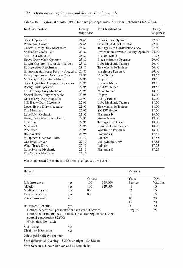
172 Open pit mine planning and design: Fundamentals
Table 2.46. Typical labor rates (2011) for open pit copper mine in Arizona (InfoMine USA, 2012).
Job Classification Hourly Job Classification Hourlywage base wage base
Shovel Operator 24.65 Concentrator Operator 22.10Production Loader 24.65 General SX-EW Operator 22.10General Heavy Duty Mechanics 23.80 Tailings Dam Construction Crew 22.10Specialists Crafts – all 23.80 Environmental/Water Facility Operator 22.10Mill Lead Operator 23.80 Reagent Mixer 21.25Heavy Duty Mech Operator 23.80 Electrowinning Operator 20.40Loader Operator (1 2 yards or larger) 23.80 Lube Mechanic Trainee 20.40Refrigeration Repairman 23.80 Tire Mechanic Trainee 20.40Environmental/Water Facility Specialist 23.80 Warehouse Person A 20.40Heavy Equipment Operator – Conc. 22.95 Mine Trainee 19.55Multi-Equip Operator – Mine 22.95 Helper 19.55Shovel Qualified Equipment Operator 22.95 Reagent Mixer 19.55Rotary Drill Operator 22.95 SX-EW Helper 19.55Truck Heavy Duty Mechanic 22.95 Mine Trainee 18.70Shovel Heavy Duty Mechanic 22.95 Helper 18.70Drill Heavy Duty Mechanic 22.95 Utility Helper 18.70MU Heavy Duty Mechanic 22.95 Lube Mechanic Trainee 18.70Dozer Heavy Duty Mechanic 22.95 Tire Mechanic Trainee 18.70Tire Mechanic 22.95 SX-EW Helper 18.70Lube P.M. Mechanic 22.95 Plantman B 18.70Heavy Duty Mechanic – Conc. 22.95 Steamcleaner 18.70Electrician 22.95 Tailings Dam Crew 18.70Machinist 22.95 Entrance Level Trainee 18.70Pipe fitter 22.95 Warehouse Person B 18.70Boilermaker 22.95 Plantman C 17.85Equipment Operator – Mine 22.10 Laborer 17.85Ore Truck Driver 22.10 Utility/Insitu Crew 17.85Water Truck Driver 22.10 Laborer 17.25Lube Service Mechanic 22.10 Plantman C 17.25Tire Service Mechanic 22.10
Wages increased 2% in the last 12 months, effective July 1,201 1.
Benefits Vacation
% paid Years DaysLife Insurance yes 100 $29,000 Service VacationAD&D yes 100 $29,000 1 10Medical Insurance yes 80 3 10Dental Insurance yes 80 5 15Vision Insurance no 10 20
15 20Retirement Benefits yes 20 20
Defined benefit: $40 per month for each year of service. 25/plus 25Defined contribution:Yes–for those hired after September 1, 2005(annual contribution $2,600)401K plan: No match.
Sick Leave yesDisability Income Ins. yes
9 days paid holidays per year.
Shift differential: Evening – $.30/hour; night – $.45/hour;
Shift Schedule: 8 hour, I0 hour, and 12 hour shifts

Mining revenues and costs 173
Table 2.47. Price of large diameter rotary blast hole drill bits (InfoMine USA, 2012).
Cutter type Diameter (inches) Unit Price ($)
Tungsten carbide 7-7/8 ea. 3,7759 ea. 5,1559-7/8 ea. 6,50110-5/8 ea. 8,09212-1/4 ea. 8,11015 ea. 16,28116 ea. 18,856
Steel tooth 7-7/8 ea. 2,6119-7/8 ea. 3,48010-5/8 ea. 4,03812-1/4 ea. 6,01615 ea. 8,48917-1/2 ea. 9,569
Table 2.48. Price of explosives and blasting accessories (InfoMine USA, 2012).
1. Bulk explosives Strength (cal/cm3) Unit Prie ($)ANFO 739 100 lb 49.05Site mixed emulsion 820–945 100 lb 46.00Repumpable emulsion 770–900 100 lb 61.32–97.10High density emulsion 815–975 100 lb 61.32–73.58
2. Non-electric shock tube millisecond delays Length (ft) Unit Price ($)8 100 258.5712 100 267.7616 100 304.5620 100 321.9530 100 401.6540 100 482.3850 100 562.1060 100 679.6380 100 875.85100 100 1031.20120 100 1211.07
3. Detonating cord Strength (grains/ft) Unit Price ($)7.5 1000 ft 134.9015 1000 ft 153.3018 1000 ft 153.3025 1000 ft 197.2540 1000 ft 226.8950 1000 ft 229.95150 1000 ft 507.93200 1000 ft 563.12
4. Cast primers Weight (lbs) Unit Price ($)1/3 ea. 2.801/2 ea. 3.573/4 ea. 3.921 ea. 4.682 ea. 8.443 ea. 12.375 ea. 20.41

174 Open pit mine planning and design: Fundamentals
Table 2.49. Capital cost mining equipment (InfoMine USA, 2012).
1. Rotary drills, electric Hole size (ins) Price ($1000)9 to 12-1/4 1,8429-7/8 to 16 2,89810-3/4 to 17-1/2 2,983
2. Graders Blade width (ft) Price ($1000)12 35914 46516 76524 1775
3. Wheel loaders Bucket capacity (yd3) Price ($1000)9 79311 1,29016 1,75218 1,77421 2,22426 4,63333 5,92453 7,652
4. Electric cable shovels (rock) Bucket capacity (yd3) Price ($1000)11 3,39716 4,45820 5,30727 8,79334 9,97555 12,655
5. Trucks, rear dump (mechanical drive) Capacity (tons) Price ($1000)40 63060 88165 89570 1,011100 1,288150 2,120170 2,517200 3,105250 3,912360 4,587380 6,050
6. Trucks, rear dump (electric drive) Capacity (tons) Price ($1000)173 2,521200 2,835280 5,583314 3,935360 6,218
7. Crawler tractors (dozers) (with ripper) Horsepower Price ($1000)260 703310 714330 735350 852410 1,047570 1,137850 2,086

Mining revenues and costs 175
REFERENCESAND BIBLIOGRAPHY
Anonymous 1909a. Monthly Average Metals Price. The Engineering and Mining Journal 88(11): 1054.Anonymous 1909b. Utah Copper Quarterly Report. The Engineering and Mining Journal 88(11): 1028.Benito, R., & S.D. Dessureault. 2008. Estimation of incremental haulage costs by mining historical data
and their influence in the final pit limit definition. Mining Engineering. 61(10): 44–49. October.Benning, I. 2000. Bankers’ perspective of mining project finance. JSAIMM. 100(3): 145–152.Berry, C.W. 1984. Economic Evaluation Phases of a Mining Prospect. Mine Feasibility – Concept to
Completion. (G.E. McKelvey, compiler). Northwest Mining Association.Bertisen, J., & G. Davis. 2007. Bias and error in mine project capital cost estimation. Paper 07-082. SMEAnnual Meeting. Feb 25–28. Denver, CO.
Bhappu, R.R., & J. Guzman. 1995. Mineral investment decision making. E/MJ. 196(7): 36–38.Bigler, L.M., & J.L. Dobra. 1994. Economic analysis of a hypothetical Mexican gold mine. E/MJ. 195(7):
16EE–16FF.Blossom, J.S. 1991. Molybdenum. 1989 Minerals Yearbook. (Volume 1): 719–728. Bureau of Mines, U.S.
Government Printing Office.BLS (Bureau of Labor Statistics) 1991. Employment, Hours, and Earnings, United States 1989–90. Bulletin
2370, vol. 1(3). U.S. Department of Labor.BLS 1992a. Productivity Measures for Selected Industries and Government Services. Bulletin 2406 (4).
U.S. Department of Labor.BLS 1992b. Producer Price. Indexes – Data for 1991 (9).BLS 1993a. Producer Price. Indexes – Data for October 1992 (2).BLS 1993b. Employment and Earnings. (6). U.S. Department of Labor.BLS 2003. Productivity for mine production and nonsupervisory workers. ftp://ftp.bls.gov/pub/special.
requests/opt/dipts/oaehhiin.txt.BLS2004a.Average hourly earnings ofmine productionworkers (SICbase). http:/www.bls.gov/data/. Series
Report. EEU10000006, EEU10100006, EEU10101006, EEU10102006, EEU10120006, EEU10122006,EEU10140006, EEU10142006.
BLS 2004b. Average hourly earnings of production workers (NAICS base). http://www.bls.gov/data/.Employment, Hours and Earnings from the Current Employment Statistics Survey (National). Createcustomized tables (one screen). Average hourly earnings of production workers, natural resources andmining, and mining (except oil and gas).
BLS 2004c. Producer price indexes for construction machinery and equipment. http://www.bls.gov/data/.Producer price index commodity data. Most requested statistics. Construction machinery and equipment.Machinery and equipment.
BLS 2004d. Labor productivity expressed in output per hour. http://data.bls.gov/PDQ/outside.jsp?/survey=ip/.
BLS 2005a. What is NAICS? http://www.bls.gov/sae/saewhatis.htmBLS 2005b. NAICS 11 & 21: Natural resources and mining. http://www.bls.gov/iag/natresmining.htmBLS2005c. CESSeries forNaturalResources andMiningUnderNAICS. http://www.bls.gov/ces/naturalres/
htm.BLS. 2012a. Bureau of Labor Statistics.
(col. A) BLS Series Report CEU1021200008, http://data.bls.gov/cgi-bin/srgate(col. B) BLS Series Report CEU1021210008, http://data.bls.gov/cgi-bin/srgate(col. C) http://www.econstats.com/blsftp/ceu102121y.htm Employment, Hours, and Earnings–National(CE) (BLS ftp ce)(col. D) http://www.econstats.com/blsftp/ceu1021230y.htm(col. E) not updated, use previous edition table reference
BLS. 2012b. Bureau of Labor Statistics.PPI Databases, Commodity Data including stage-of-processing indexes.One-Screen Data Search, Machinery and Equipment (code 11), Construction machinery and equipment(code 112), Not seasonally adjustedOrProducer Price Indexes, Series Reports, WPU112 http://www.bls.gov/ppi/
BLS. 2012c. Bureau of Labor Statistics. Productivity and Costs, LPC Databases, Industry Productivity andCosts, One Screen Data Search. http://www.bls.gov/lpc/#tables

176 Open pit mine planning and design: Fundamentals
Bourne, H.L. 1994. What it’s worth: A review of mineral royalty information. Mining Engineering. 46(7):641–644.
Bourne, H.L. 1995. What it’s worth: A review of mineral royalty information. Mining Engineering. 47(7):654–657.
Bourne, H.L. 1996. What its worth: A review of mineral royalty information. Mining Engineering. 48(7):35–38.
Camm, T.W. 1991. Simplified cost models for prefeasibility mineral evaluations. USBM. InformationCircular 9298.
Camm, T.W. 1994. Simplified cost models for prefeasibility mineral evaluations. Mining Engineering.46(6): 559–562.
Camus, J. 2002. Management of mineral resources. Mining Engineering. 54(1): 17–25.Camus, J.P. 2002. Management of Mineral Resources: Creating Value in the Mining Business. SME.
Littleton, Colorado. 107 pages.Cavender, B. 2001. Leadership vsmanagement: Observations on the successes and failures of cost-reduction
programs. Mining Engineering. 53(8): 45–50.Cherrier, T.E. 1968. A Report on the Ceresco Ridge Extension of the Climax Molybdenite Deposit.
MSc. Thesis. University of Minnesota.CMJ (Canadian Mining Journal) 1986. Reference Manual and Buyers Guide. Southam Business
Publications.CMJ 2004. Mining Source book. Canadian Mining Journal. www.canadian mining journal.comCMJ 2010. Canadian Mining Journal, 2010 Mining Sourcebook.Coal Age 1992. Buyers Guide. Maclean Hunter Publication (6): 57–107.Cost Reference Guide. 2012. Equipment Watch, a Penton Media brand. NewYork City, NY.Crowson, P. 2011. Copper focus – The copper conundrum. Mining Magazine. November. pp. 14–21.Dataquest Inc.Cost ReferenceGuide for Construction Equipment. PaloAlto, Calif.: Equipment Guide-Book
Company.Davis, G. 1996. Using commodity price projections in mineral project valuation. Mining Engineering.
48(4): 67–70.Davis, G. 1998. One project, two discount rates. Mining Engineering. 50(4): 70–74.Davis, G.A. 1995. (Mis)use ofMonteCarlo simulations inNPVanalysis. MiningEngineering. 47(1): 75–79.Dixon, S. 2004. Definition of economic optimum for leaching of high acid consuming copper ores. Pre-print
Paper 04-04. 2004 SMEAnnual Meeting, Feb 23–25. Denver, CO.Dran, J.J. Jr. & H.N. McCarl 1977. An examination of interest rates and their effect on valuation of mineral
deposits. Mining Engineering 29(6): 44–47.Dysinger, S.M. 1997. Capital budgeting: forecasting the future. Mining Engineering. 49(9): 35–38.E/MJ 1986. Average Annual Metal Prices. 1925–1985 (3) 27.E/MJ 1992. Buyers Guide 1992. E&MJ 193(10): BG1-45.E/MJ 1993. Prices from the American Metal Market. Friday January 15, 1993: 74WW.Emery, X., &A. Cabañas. 2004. Forecasting copper prices in the short andmedium terms using geostatistics.
CIM Magazine. September. pp. 42–53.Engineering News Record (ENR). 2012. Historical Cost Indices. http://enr.construction.com/economics/
historical_indices/ENR (Engineering News Record) 1976–1992. Annual Summary.ENR 1993. ENR Market Trends. (2).ENR 2005. ENR’s Cost Indexes. www.enr.com.Equipment Quest. 2003. Cost Reference Guide for Construction Equipment. Primedia Publications.Ericsson, M., Löf, A., & O. Östensson. 2010. Iron ore review, 2009–2010: New pricing, tight supplies, and
China’s steel output defined the market. E/MJ. 211(8): 28–34. October.Finlay, J.R. 1908. Cost of producing the world’s supply of copper. The Engineering and Mining Journal
86(7): 165–168.Finlay, J.R. 1909. Cost of pig iron made from Lake Superior ores. The Engineering and Mining Journal
87(15): 739–745.Frimpong, S. & J.M. Whiting. 1996. The pricing of mineral investment options in competitive markets.
In Surface Mining 1996 (H.W. Glen, editor): 37–42. SAIMM.Gallagher, T.C. 1982. Developing a construction cost escalation index for the U.S. mining and metals
industry. Cost Engineering 24(3): 147–152.

Mining revenues and costs 177
Gentry, D.W. 1988. Minerals project evaluation – An overview. Trans. Instn. Min. Metall. (Sect. A: Min.Industry) 97(1): A25–A35.
Gentry, D.W. 1998. 1998 Jackling Lecture: Constrained prospects of mining’s future. Mining Engineering.50(6): 85–94.
Hajdasinski, M.M. 1993. A generalized true rate of return of a project. 24th International Symposiumon Application of Computers and Operations Research in the Mineral Industry: 2(280–287). Montreal:CIMM.
Hajdasinski, M.M. 2000. Internal rate of return (IRR) – a flawed and dysfunctional project evaluationcriterion. Mining Engineering. 52(8): 49–56.
Hajdasinski, M.M. 2000. Internal rate of return (IRR) as a project-ranking tool. Mining Engineering.52(11):60–64.
Hansen, B.D. 1999. Reducing Newmont’s operating costs and increasing reserves and production at amid-sized international mining company. Pre-print Paper 99-031. 1999 SMEAnnual Meeting, Mar 1–3.Denver, CO.
Hart, W.M. 2006. 2006. Building high performance teams and enhancing cash flow. Paper 06-011. SMEAnnual Meeting. Mar 26–29. St. Louis, MO.
Heath, K.C.G. 1988. Mine costing. Trans. Inst. Min. Metall. (Sect. A: Min. industry) 97(1): A1–A8.Hrebar, M.J. 1977. Financial analysis Mineral Industry Costs. (J.R. Hoskins & W.R. Green, editors):
205–224. Northwest Mining Association.Hummel, R. 2001. The road to NPV+. JSAIMM. 101(8): 411–420.Humphreys, D. 1989. The metal markets since 1983 – and into 1989. International Mining 6(1):
14–22.Huss, M.P. 1984. Marketing planning.Mine Feasibility Concept to Completion (G.E. McKelvey, compiler).Northwest Mining Association.
IMF, 2012. International Monetary Fund, Primary Commodity Prices www.imf.org/external/np/res/commod/index.aspx www.indexmundi.com/commodities/?commodity=iron-ore&months=120
IMF. 2012. International Monetary Fund. www.indexmundi.com/commodities/?commodity=iron-ore&months=360
Industrial Minerals, 1992. Prices. 303(12): 66.Industrial Minerals. 2012. Monthly Prices, June 2012. www.indmin.comInfoMine USA, 2012. Mining Cost Service. Periodically updated. Spokane, WA. Available from http://
www.costs/infomine.comIRS (U.S. Internal Revenue Service) 1988a. Business Expenses. Publication 535 (Rev. Nov. 88).IRS 1988b. Depreciation. Publication 534. (Rev. Nov. 88).IRS 2004. Publication 535 (2004) Business Expenses. http://www.irs.gov/publications/p535/ch10.htmlIRS 2004. Publication 946 (2004): How to Depreciate Property. http://www.irs.gov/publications/p946/
index.htmlIRC 2004C. Publication 535 (2004): Depletion. http://www.irs.gov/publications/P535/ch10.htmlIRS 2011. Internal Revenue Service. Depletion. www.irs.gov/publications/p535/ch09.htmlJackling, D.C. 1909. Operations of Utah Copper Co. During 1908. The Engineering and Mining Journal
88(6): 1185–1188.Ji, C. & Y. Zhang. 1999. Gray-correlation analysis of production cost. 28th International Symposium onApplication of Computers and Operations Research in the Mineral Industry: 173–176. Colorado Schoolof Mines: CSM.
Jolly, J.L.W. & D.L. Edelstein 1991. Copper. 1989 Minerals Yearbook. (Volume 1): 333–386. Bureau ofMines. U.S. Government Printing Office.
Kirkman, R.C. 1979. Discussion of the H.M. Wells paper. Mining Engineering 31(4): 406–407.Kirk, W.S. 1998. Iron ore reserves and mineral resource classification systems. Skillings Mining Review.
June 6. pp. 4–11.Kitco 2005. Charts and Data. http://www.kitco.com/scripts/hist_charts/yearly_graphs.cgiKovisars, L. 1983. Mine and mill labor productivity study shows wide range of values.Mining Engineering
36(11): 1536–1537.Kuck, P.H. &C.M. Cvetic 1991. Iron ore. 1989Minerals Yearbook. (Volume 1): 521–564. Bureau ofMines,
U.S. Government Printing Office.Labys, W.C. 1977. Minerals commodity modeling – the state of the art. Mineral Policies in Transition.
(J.H. DeYoung, Jr., editor). The Council of Economics of AIME (11): 80–106.

178 Open pit mine planning and design: Fundamentals
Laing, G.J.S. 1976.AnAnalysis of the Effects of State Taxation on theMining Industry In the RockyMountainStates.MSc. Thesis T-1900. Colorado School of Mines.
Lawrence, M.J. 2000. DCF/NPV modeling: Valuation practice or financial engineering? Pre-print Paper00-58. 2000 SMEAnnual Meeting, Feb 28–Mar 1. SLC, UT.
Lawrence, R.D. 2000. Should discounted cash flow projections for the determination of fair market valuebe based solely on proven and probable reserves? Pre-print Paper 00-64. 2000 SME Annual Meeting,Feb 28–Mar 1. SLC, UT.
Lawrence, R.D. 2001. Should discounted cash flow projections for the determination of fair market valuebe based solely on proven and probable reserves. Mining Engineering. 53(4): 51–56.
Lesemann, R.H. 1977. Commercial and price considerations in mine feasibility and cost studies. MineralIndustry Costs. (J.R. Hoskins &W.R. Green, editors): 195–204. Northwest Mining Association.
Lewis, F.M., Chase, C.K. & R.B. Bhappu. 1978. Copper production costs update. Mining Engineering30(4): 371–373.
Lewis, P.J. & C.G. Streets 1978. An analysis of base-metal smelter terms. Proceedings of the 11th Commonwealth Mining and Metallurgical Congress: 753–767. Hong Kong: IMM.
Lillico, T.M. 1973. How to maximize return on capital when planning open pit mines.World Mining 9(6):22–27.
LKAB. 2005. Personal communication. www.lkab.comLong, K. 2011. Statistical methods of estimating mining costs. Paper 11-023. SME Annual Meeting.
Feb 27–Mar 2. Denver, CO.Manssen, L.B. 1983. Financial evaluation of mining projects: Is ‘common practice’ enough? Mining
Engineering 35(6): 601–606.Mason, P.M. 1984. Capital and operational planning for open pit in a modern economy. 18th International
Symposium on Application of Computers and Mathematics in the Mineral Industry: 791–802. London:IMM.
Metal Bulletin 1993. Metal Prices (1). Trans-world Metals (USA) Ltd.Metal Bulletin 2004. www.metalbulletin.com. Personal communication.Metal Bulletin 2012. Personal communication. http://www.metalbulletin.comMetals Bulletin 2012. Personal communication. http://www.metalbulletin.comMetals Week 1993. Weekly Prices (2).Metals Week 2005. July. www.plats.com.Miner, R.B. 2003. Using long-term international concentrate agreements in major project financing. CIM
Bulletin 96(1074): 56–64.Mining Cost Service 1989. Model Smelter Schedules. Spokane, WA: Western Mine Engineering.Mining Cost Service 1992. Prices for Large Diameter Blast Hole Bits. Spokane, WA: Western Mine
Engineering.Mining Sourcebook 2004. Canadian Mining Journal. www.canadianminingjournal.comMireku-Gyimah, D.& J.O. Darko. 1996. Economic risk analysis ofmineral projects inGhana –A simulation
approach. In Surface Mining 1996 (H.W. Glen, editor): 71–76. SAIMM.Mular, A.L. 1978. Mineral Processing Equipment Costs and Preliminary Capital Cost Estimates. SpecialVolume 18. CIM.
Mular,A.L. 1982. Mining andMineral Processing Equipment Costs and Preliminary Capital Cost Estimates.Special Volume 25. CIM.
Mular, A.L. & R. Poulin. 1998. CAPCOSTS: A Handbook for Estimating Mining and Mineral ProcessingEquipment Costs and Capital Expenditures and Aiding Mineral Project Evaluations. Special Volume 47.CIM.
Murdy, W.W., & R.R. Bhappu. 1997. Risk mitigation in global mining development. Mining Engineering.49(9): 30–34.
Nangolo, C., & C. Musingwini. 2011. Empirical correlation of mineral commodity prices with exchange-traded mining stock prices. JSAIMM. 111(7): 459–468.
Neretin, A.V. 2007. Cost/Performance Evaluation of Gold Placer Mining Methods – For a Range ofGold Placer Deposits in the Bodaibo District, Russia, AUSIMM Conference Proceedings, World GoldConference Cairns, QLD, October 2007, pp. 57–65.
Noble, A.C. 1979. Price forecasting and sensitivity analysis for economic analysis of final pit limit.Open Pit Mine Planning and Design (J.T. Crawford and W.A. Hustrulid, eds): 127–133. New York:SME-AIME.

Mining revenues and costs 179
O’Hara, T.A. 1980. Quick guides to the evaluation of orebodies. CIM Bulletin (no. 814) 73(2):87–99.
O’Hara, T.A. 1981. Chapter 6: Mine evaluation. Mineral Industry Costs (J.R. Hoskins, compiler): 89–99.Northwest Mining Association.
O’Hara, T.A. & S.C. Suboleski 1992. Chapter 6.3: Costs and cost estimation. SME Mining EngineeringHandbook 2nd Edition (Volume 1) (H.L. Hartman, Senior Editor): 405–424. SME.
O’Neil, T.J. 1982. Mine evaluation in a changing investment climate (Parts 1 and 2). Mining EngineeringPart 1 vol. 34(11): 1563–1566, Part 2, vol. 34(12): 1669–1672.
Osborne, T.C. 1985. What is the cost of producing copper? International Mining 2(3): 14–15.Paulsen, K.R. 1981. Environmental and regulatory costs of mining projects. Mineral Industry Costs
(J.R. Hoskins, compiler): 27–32. Northwest Mining Association.Petersen, U. & R.S. Maxwell. 1979. Historical mineral production and price trends. Mining Engineering
31(1): 25–34.Pfleider, E.P. & G.F. Weaton. 1968. Chapter 13.4: Iron ore mining. Surface Mining (E.P. Pfleider, editor):
917–921. NewYork: AIME.Pierson, G. 1997. Commodity prices from a monetary perspective. Mining Engineering. 49(10): 75–80.Platts Metals Week, 2012. Weekly Metal Prices, April 16, 2012. The McGraw Hill Companies.
http://www.platts.com/Products/metalsweekPRIMEDIA 2004. Cost Reference Guide for Construction Equipment. Primedia Publications.Randal, R.L. 1979. Economic modeling and market forecasting Computer Methods for the ’80’s: 938–949.
Society of Mining Engineers of AIME.Randall, R.L. 1980. Sources of cyclical variation in the mineral industries. Proceedings of the Council of
EconomicsAIME: 11–118.Rendu, J-M. 2003. SME meets with the SEC – resources and reserves reporting discussed. Mining
Engineering. July. P35.Roberts, M.C. 2000. Cycles in mineral prices. Pre-print Paper 00-73. 2000 SME Annual Meeting, Feb
28–Mar 1. SLC, UT.Roberts, M.C. 2002. Cycles in metal prices. Mining Engineering. 54(2): 40–48.Rosta, J. 1992. Gold, silver. Mining Engineering 44(5): 449.Runge, I.C. 1998. Mining Economics and Strategy. SME. Littleton, Colorado. 295 pages.Silver, D. 2008. Super Cycle: past, present and future. Mining Engineering. 60(6): 72–77. June.Simonsen, H. & J. Perry. 1999. Risk identification, assessment and management in the mining and
metallurgical industries. JSAIMM. 99(6): 321–328.Skillings Mining Review 1993a. Iron Ore Prices. 82(2).Skillings Mining Review 1993b. Rail Freight Rates on Iron Ore and Pellets Per Gross Ton. 82(2).Skillings Mining Review 1993c. Rail and Lake Tariff Rates on Iron Ore and Pellets PerGross Ton.
vol. 82(2).Skillings 2005. Metal/ore prices. August www.skillings.net.Smith, L.D. 1999. The argument for a “bare bones” base case. CIM Bulletin 92(1031): 143–150.Soderberg, A. 1930.Mining method and costs at the Utah Copper Co., Bingham Canyon, Utah. US Bureau
of Mines Information Circular 6234.Soma, J.L. 1977. Estimating the cost of development and operating of surface mines. Mineral Industry
Costs (J.R. Hoskins &W.R. Green, editors): 67–90. Northwest Mining Association.Southam Mining Group 1993. Mining Source Book. Southam Mining Group. Don Mills, Ontario.Staff 1987. Bureau of Mines Cost Estimating System Handbook. Part 1. Surface and Underground Mining.
U.S. Bureau of Mines Information Circular 9142: 631 pages.Staff 1987. Bureau of Mines Cost Estimating System Handbook. Part 2. Mineral Processing. U.S. Bureauof Mines Information Circular 9143: 566 pages.
Stebbins, S. 2002. Evaluating the economics of development alternatives early in the project feasibilityprocess. 30th International Symposium on Application of Computers and Operations Research in theMineral Industry: 587–600. Alaska: SME.
Stermole, F.J. 1979. Economic evaluation of open pit mines. Open Pit Mine Planning and Design(J.T. Crawford & W.A. Hustrulid, editors): 136–144. New York: Society of Mining Engineers of theAIME.
Stermole, F.J., & J.M. Stermole. 2012. Economic Evaluation and Investment Decision Methods. (13thedition). Investment Evaluations Corporation.

180 Open pit mine planning and design: Fundamentals
Stermole, F.J., & J.M.Stermole 1987. EconomicEvaluation and InvestmentDecisionMethods. (6thEdition).Investment Evaluations Corporation.
Stinnett, L.A., & J.A. Wehinger. 1995. Labor productivity and its impact on product price. MiningEngineering. 47(7): 658–659.
Taylor, H.K. 1977. Mine valuation and feasibility studies. Mineral Industry Costs: 1–17. Spokane, WA:Northwest Mining Association.
Taylor, H.K. 1988. Discussion of the article ‘Mine Costing’ by K.G.G. Heath. Trans. Inst. Min. Metall.(Sect A: Min industry) 97(10): A196–197.
Taylor, H.K. 1992. Private communication.Tilton, J.E. 1997. Surviving in the competitive and global mining industry. Mining Engineering. 49(9):
27–29.Torries, T.F. 1998. NPV or IRR? Why not both? Mining Engineering. 50(10): 69–73.Ulatowski, T. 1982. Inflationary impacts on project evaluation; real and nominal hurdle rates. Mineral
Industry Costs (J.R. Hoskins, compiler): 245–248. Northwest Mining Association.U.S. Bureau of the Census 1992. Statistical Abstract of the United States. (112th edition)Washington, D.C.U.S. Census Bureau. 2005. 1997NAICSMatched to 1987 SIC –Mining. http://www.census.gov/epcd/naics/
NAICS21.htm.USGS. 2005a. Aluminum Statistics and Information. http://minerals.usgs.gov/minerals/pubs/commodity/
aluminum/.USGS. 2005b. Copper Statistics and Information. http://minerals.usgs.gov/minerals/pubs/commodity/
copper/.USGS. 2005c. Lead Statistics and Information. http://minerals.usgs.gov/minerals/pubs/commodity/lead/.USGS. 2005d. Zinc Statistics and Information. http://minerals.usgs.gov/minerals/pubs/commodity/zinc/.USGS. 2005e. Gold Statistics and Information. http://minerals.usgs.gov/minerals/pubs/commodity/gold/.USGS. 2005f. Platinum-Group Metals Statistics and Information. http://minerals.usgs.gov/minerals/pubs/
commodity/platinum/.USGS. 2005g. Silver Statistics and Information. http://minerals.usgs.gov/minerals/pubs/commodity/silver/.USGS. 2005h.MolybdenumStatistics and Information. http://minerals.usgs.gov/minerals/pubs/commodity/
molybdenum/.USGS. 2005i. Nickel Statistics and Information. http://minerals.usgs.gov/minerals/pubs/commodity/nickel/.USGS. 2005j. Tin Statistics and Information. http://minerals.usgs.gov/minerals/pubs/commodity/tin/.USGS. 2005k. Iron Ore Statistics and Information. http://minerals.usgs.gov/minerals/pubs/commodity/
iron_ore/.USGS. 2005l. Historical statistics for mineral and material commodities in the United States.
http://minerals.usgs.gov/minerals/pubs/of01-006/.USGS. 2005m. Metal prices in the United States through 1998. http://minerals.usgs.gov/minerals/pubs/
metal_prices/.USGS. 2012a, U.S. Geological Survey, Mineral Commodity Summaries, 2012 http://minerals.usgs.gov/
minerals/pubs/mcs/.USGS. 2012b, U.S. Geological Survey, Data Series 140, Historical Statistics for Mineral and Material
Commodities in the United States, Iron Ore, 2012 http://minerals.usgs.gov/ds/2005/140/.Viera, F.M. 1993. How to choose projects bymeans of risk analysis. 24th International Symposium onAppli-
cation of Computers and Operations Research in the Mineral Industry: 2(324–331). Montreal: CIMM.Walker, S. 2005. Management in action – Surface costs: Keeping mining costs at bay. Mining Magazine.
October. pp. 28–34.Warnken, D.E. 2005. A case study in valuation of non-producing mineral rights. Pre-print Paper 05-113.
2005 SMEAnnual Meeting, Feb 28–Mar 2. SLC, UT.Wells, H.M. 1978. Optimization of mining engineering design in mineral valuation. Mining Engineering
30(12): 1676–1684.Werner, A.B.T. & C. Janakiraman. 1980. Smelter contracts and their place in mineral reserve evaluation.
Proceedings of the Council of EconomicsAIME: 85–92.Western Mine Engineering 2003. Mine and Mill Equipment Costs – Estimator’s Guide.Western Mine Engineering 2004. Mining Cost Service.Williamson, D. 1997. Into the next millennium – The long bull market in minerals. Mining Engineering.
49(6): 61–64.World Steel Association. 2012. www.worldsteel.org

Mining revenues and costs 181
Wright, E.A. 1993. A simulation model for assessing mining investment incentives. 24th InternationalSymposium onApplication of Computers and Operations Research in the Mineral Industry: 2(332–342).Montreal: CIMM.
Yernberg, W.R. 2000. Copper 99: Mine closures help copper prices improve. Mining Engineering. 52(1):36–36.
Yernberg, W.R. 2008. Copper mining industry in Arizona is expanding. Mining Engineering. 60(3): 41.March.
Zhang, M., Stone, P., Middleton, R., & M. Menabde. 2007. A study of the impact of price uncertainty tomining project valuation. Paper 07-054. SMEAnnual Meeting. Feb 25–28. Denver, CO.
ACKNOWLEDGEMENTS
The authors would like to express their appreciation to:1. Ms. Jennifer Leinart, Cost Mine Division Director, InfoMine USA2. Ms. Karen McBeth, Editorial Director, Metals Pricing and Market Engagement, Platts
Metals group3. Ms. Mary Higgins, Prices Department Manager, Metal Bulletin4. Charles Pitts, Editor, Skillings Mining Review5. Robert Seagraves, Publisher, Canadian Mining Journal/Mining Source Book6. Frank Stermole, Investment Evaluations Corporation7. Mike O’Driscoll, Editor, Industrial Minerals8. Scott Lewis, Editorial Research Director, Engineering News-Letter9. Garrett Schemmel, Director, BrandManagement, EquipmentWatch/PentonMedia Inc.
10. Ms. April LeBlond, Customer Support Coordinator, Penton Media Inc.11. The World Steel Associationfor permission to include materials from their publications in this 3rd edition.
REVIEW QUESTIONSAND EXERCISES
1. What is meant by the term “future worth”?2. What is meant by the term “present value”?3. Assume that the interest rate is 5% compounded daily. What would be the equivalent
simple interest rate?4. If $1000 is placed in a bank savings account earning 5% annually, what is the value
after 10 years?5. Would you rather have $10,000 today or $20,000 in 5 years? Assume an interest rate
of 8%.6. Would you rather have $10,000 today or receive payments of $ 1000/year for the next
20 years?7. What is meant by the term ‘payback period’?8. If you borrowed $10,000 from the bank today, how long would it require to repay the
loan at $1000/year? Interest rate of 5%.9. What is meant by the term ‘rate of return’?
10. You invest $1000 today. It will be repaid in 15 equal payments of $200 over a periodof 15 years. What is your rate of return? If you could put the money in a certificate ofdeposit paying 5%, what should you do?

182 Open pit mine planning and design: Fundamentals
11. What is meant by the term ‘cash flow’?12. Redo the cash flow example in Table 2.1 assuming that the capital cost in year 0
was – $300 and in year 1 was – $200. What is the total cash flow?13. For problem 12, using a discounting rate of 15%, what is the net present value?14. What is meant by the term ‘discounted cash flow’?15. What is meant by the term ‘discounted cash flow rate of return’?16. For problem 12, what is the DCFROR?17. Redo the cash flow example in Table 2.2 assuming that the capital cost in year 0 is
$150 rather than $100.18. What is meant by depreciation? How is it included in a cash flow calculation?19. Redo the example in section 2.2.9 assuming that the salvage value is $50.00.20. What is meant by the ‘depletion allowance’?21. What are the two types of depletion? Describe how they differ.22. How is depletion included in a cash flow calculation?23. Redo the cash flow including depletion example given in section 2.2.1 assuming a
nickel ore rather than silver.24. What are the different factors that must be considered when performing a cash flow
analysis of a mining property?25. What is the weight of a
– short ton– metric ton– long ton
26. What is meant by the expression ‘long ton unit’? Short ton unit? Metric ton unit?Provide an example of a mineral which is sold in this way.
27. Assume that the price for iron ore fines is 45 g U.S./mtu. What is the value of aconcentrate running 63.45% Fe?
28. How much is a troy ounce? What metals are sold by the troy ounce?29. How is mercury sold?30. In what form is molybdenum normally sold?31. What is meant by FOB? What is meant by C.I.F.? Why is it important that you
understand the meaning of these terms?32. Select a metal from Table 2.6 and determine the price today.33. Select a non-metal from Table 2.7 and determine the price today.34. Select an ore from Table 2.8 and determine the price today.35. Compare the price of the Cleveland-Cliffs, Inc. iron ore pellets given in Table 2.9 with
the price today.36. Table 2.10 gives the rail tariff rates for iron ore and pellets. Try to find similar rail tariff
data which are applicable today.37. Table 2.11 gives the lake freight tariff rates for iron ore and pellets. Try to find similar
data which are applicable today.38. What are the primary uses of cobalt? Using values from Platt’s Metals Week, plot the
price history over the past 5 years.39. What are the primary uses of barytes? Using values from Industrial Minerals, plot the
price history over the past 5 years.40. Tables such as shown in Table 2.14 are no longer published by the Skillings Mining
Review. However, their “Iron Ore Price Report” provides the prices for the Minnesota

Mining revenues and costs 183
and Michigan products of Cliffs Natural Resources, Inc. Using this resource, plot thedevelopment of the prices over the past 5 years.
41. Select a metal fromTable 2.15 and plot the price versus time. Describe the price patternobserved. Try to attribute reasons for the major fluctuations observed.
42. Using the endpoint data in problem 41, what would be the average annual percent priceincrease?
43. Using the data in problem 41, predict what the price might be in 5 years, 10 years and20 years in the future.
44. Plot the data from Table 2.16 for the same metal selected in problem 41. Describe theprice patternwith time.What reasons canyouprovide, if any, for themajorfluctuations?
45. Using the data from problem 44, what price might you expect in 1 year, 5 years, 10years and 20 years?
46. The price of iron ore fines is given in Table 2.17 for the period 1900 through 2010. Plotthe data from the year that you were born until today. Any explanation for the pattern?
47. Table 2.18 presents the monthly spot price for iron ore fines, 62% Fe (China importCFR Tianjin port) expressed in US $/metric ton. These values have been plotted inFigure 2.7. Discuss the curve and its significance.
48. Table 2.19 presents the annual steel production (in thousand tonnes) for the top twentysteel producing countries for years 2000 to 2011 ranked by year 2011 production.Thedata are providedby theWorldSteelAssociation. Thedata for the topfiveproducersare plotted in Figure 2.8. What does Figure 2.8 show?Your conclusion?
49. Trend analysis is one way to predict future prices based upon historical data but it mustbe carefully done. To illustrate the types of problems that can occur, select one of themetal price – time data sets for analysis. Fit a second order polynomial to the data.Fit a third order polynomial to the data. Fit an arbitrary higher order polynomial to thedata. Compare the results obtained using each equation if you extrapolate 5 years, 10years and 20 years into the future? What are your conclusions?
50. What is the difference between extrapolation and interpolation?51. What is meant by an econometric model?When applied in mining, what factors might
be included?52. What is meant by ‘net smelter return’? How is it calculated?53. What are the major elements of a smelter contract?54. What is meant by ‘at-mine-revenue’? Why is it important?55. Redo the example in section 2.3.5 using the Model Smelter Schedule given in
Table 2.24. Make the necessary assumptions.56. What are some of the different cost categories used at a mining operation? Describe
the costs included in each.57. What is meant by ‘general and administrative’ cost? What does it include?58. How might the operating cost be broken down?59. What are meant by fixed costs? Should they be charged to ore, waste, or both?60. Discuss the value of information such as contained inTable 2.25 to a student performing
a senior pre-feasibility type analysis.61. Table 2.25 presents the mining costs at the Similkameen operation. Determine a
percentage distribution. Present these costs in a pie-type plot.62. Compare the information presented in Tables 2.25 and 2.26 for the Similkameen/
Similco operation.

184 Open pit mine planning and design: Fundamentals
63. What is the value of data such as contained in Table 2.26?64. Compare the Similkameen and Huckleberry mines based upon the data provided in
Tables 2.25 and 2.27.65. The Canadian Mining Journal ceased production of its Mining Sourcebook with the
2010 edition. Hence, Table 2.28 is the last one of its type. Outline the type of infor-mation contained in the table. Identify some other sources where one might find thesetypes of data. Choose one of the mines in the table and find the equivalent data fromanother source.
66. In section 2.4.3, the estimation of costs based upon the escalation of older costs isdescribed. Estimate the cost of the building in year 2011 based upon the different ENRindices. Which value do you think might be the most appropriate? Why?
67. Select one of the categories in Table 2.30.What was the average annual percent hourlywage increase over the period 1970 to 1980? Over the period 1980 to 1990? Over theperiod 1990 to 2000? On this basis, what would you predict it to be in 2000 to 2010?What was it?
68. What was the reason to change from the SIC to the NAICS base?69. Using Table 2.32, how much would you estimate the price of a mining truck has
increased over the past 10 years?70. Why is it important to include the change in productivity when escalating older costs?
How can you do this?71. In 1980, O’Hara published the curve relating mine/mill project capital cost to the
milling rate. Discuss how you might try to produce a similar curve today.72. Actual data for a number of open pit mining operations have been provided in Tables
2.25, 2.26, 2.27 and 2.28. Compare some of the estimates from section 2.4.5 with theseactual data.
73. Discuss how the curves included in section 2.4.5 might be updated.74. Compare the mine and mill operating costs predicted using the O’Hara estimators with
the actual costs given in Tables 2.25, 2.26, 2.27 and 2.28.75. A detailed cost calculation has been provided in section 2.4.6. Repeat the example but
assume that the ore and waste mining rates are twice those given.76. In section 2.4.7 a ‘quick-and-dirty’ mining cost estimation procedure has been pro-
vided. Sometimes it is possible to obtain a percentage cost breakdown for a miningoperation even if the actual costs are unavailable. How might such a cost distributionbe beneficial?
77. Apply the quick-and-dirty approach to the Similkameen data.78. Apply the quick-and-dirty approach to the Huckleberry data.79. Some detailed cost information is provided in section 2.4.8. Using the data in Table
2.44, what might be the expected purchase price of a Bucyrus-Erie 59-R drill?80. When using published costs and/or cost estimators it is very important to know what is
included. In Table 2.44, describe the basis/meaning for the different cost components.81. What are typical depreciation lives for mining equipment (trucks, shovels, drills, front
end loaders, graders, dozers, pickup trucks, etc.)?82. What items are included in equipment ownership costs? What is the approximate split
between ownership and operating cost for a piece of equipment?83. Assume that you have a small equipment fleet consisting of
– Caterpillar D9T dozer (1)– Caterpillar 992K wheel loader (1)

Mining revenues and costs 185
– Caterpillar 777F trucks (3)– Caterpillar 16M grader (1)– Atlas Copco Pit Viper 271 drill (1)Whatwould be the expected total hourly operating cost? Does this include the operator?
84. Using the values given in Table 2.46, what would be the cost of the operators to runthe equipment in problem 83?
85. TheAtlas Copco Pit Viper 271 drill will complete a 7-7/8′′ diameter hole, 40 ft long in40 minutes. The life of the tungsten carbide cutter is 5000 ft. What is the cost of eachhole?
86. Except for 10 ft of stemming, the hole in problem 85 is filled with ANFO. One 1/3 lbprimer is used and the downline is detonating cord (15 grains/ft). What would be thecost of explosive per hole.
87. For the fleet described in problem 83, what would be the approximate capital costbased upon the information contained in Table 2.49?

CHAPTER 3
Orebody description
3.1 INTRODUCTION
Today, most potential orebodies are explored using diamond core drilling. The small diam-eter core collected from each hole provides a continuous ‘line’ of geologic information.Each of the recovered cores is studied in detail and the contained information recorded. Theprocess is called ‘logging’. Each ‘line’ is subsequently subdivided into a series of segmentsrepresenting a particular rock type, structural feature, type of mineralization, grade, etc. Bydrilling a pattern of such holes, a series of similarly segmented lines are located in space.Using this information, together with a knowledge of the geologic setting and other factors,the mining geologist proceeds to construct a 3-dimensional representation of the mineral-ized body. The objective is to quantify, as best possible, the size, shape and distribution ofthe observable geologic features. The distribution of ore grades are correlated to lithology,alteration, structure, etc. The result is a mineral inventory or geological reserve. At this pointin the evaluation process, economics have not been introduced so that terms such as ‘ore’or ‘ore reserve’ are not involved.
The development of a mineral inventory involves substantial judgement, assumptionsbeing made regarding sample and assay quality, and the interpretation and projection ofgeologic features based upon very limited data. The geologic data base, properly gatheredand interpreted, should remain useful for many years. It forms the basis for current andfuture feasibility studies, mine planning and financial analyses. The success or failure of aproject can thus be directly linked to the quality of its recorded data base, the drill logs andthe maps. This chapter covers some of the basic techniques involved in the developmentand presentation of a mineral inventory.
3.2 MINE MAPS
The fundamental documents in all stages of mine planning and design are the maps.Maps are essential for the purpose of:
– collecting,– outlining, and– correlating
a large portion of the data required for a surface mining feasibility study. These maps aredrawn to various scales. The ‘scale’ is the ratio between the linear distances on the map and
186
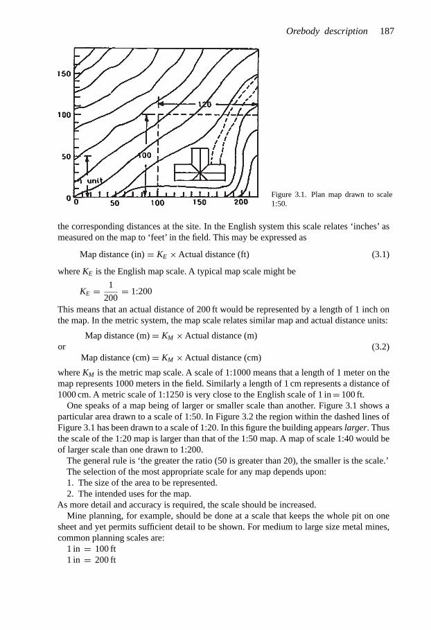
Orebody description 187
Figure 3.1. Plan map drawn to scale1:50.
the corresponding distances at the site. In the English system this scale relates ‘inches’ asmeasured on the map to ‘feet’ in the field. This may be expressed as
Map distance (in) = KE × Actual distance (ft) (3.1)
where KE is the English map scale. A typical map scale might be
KE = 1
200= 1:200
This means that an actual distance of 200 ft would be represented by a length of 1 inch onthe map. In the metric system, the map scale relates similar map and actual distance units:
Map distance (m) = KM × Actual distance (m)or
Map distance (cm) = KM × Actual distance (cm)(3.2)
where KM is the metric map scale. A scale of 1:1000 means that a length of 1 meter on themap represents 1000 meters in the field. Similarly a length of 1 cm represents a distance of1000 cm. A metric scale of 1:1250 is very close to the English scale of 1 in = 100 ft.
One speaks of a map being of larger or smaller scale than another. Figure 3.1 shows aparticular area drawn to a scale of 1:50. In Figure 3.2 the region within the dashed lines ofFigure 3.1 has been drawn to a scale of 1:20. In this figure the building appears larger. Thusthe scale of the 1:20 map is larger than that of the 1:50 map. A map of scale 1:40 would beof larger scale than one drawn to 1:200.
The general rule is ‘the greater the ratio (50 is greater than 20), the smaller is the scale.’The selection of the most appropriate scale for any map depends upon:1. The size of the area to be represented.2. The intended uses for the map.
As more detail and accuracy is required, the scale should be increased.Mine planning, for example, should be done at a scale that keeps the whole pit on one
sheet and yet permits sufficient detail to be shown. For medium to large size metal mines,common planning scales are:
1 in = 100 ft1 in = 200 ft

188 Open pit mine planning and design: Fundamentals
Figure 3.2. A portion of the plan map in Figure 3.1 drawn to scale 1:20.
In the metric system, common scales are:1:10001:12501:2000
Geologic mapping is commonly done on a larger scale such as 1 in = 40 ft (the correspondingmetric scale is 1:500). For planning purposes, the geologic features (outlines) are replottedonto the smaller scale maps.
The types of maps prepared and used depends upon the stage in the life of the property. Atthe exploration stage, satellite maps may provide important information regarding structuralregimes and potential exploration sites. These can be complemented with infra-red photos,etc. For certain types of information, for example the location of smelters, a small scalemap, such as a map of the U.S., may be the most appropriate. Certain materials, such ascrushed rock, are highly dependent on transportation costs. Regional maps overlain withcircles corresponding to different freight tariffs are useful for displaying potential markets.
A state map Figure 3.3 can provide a considerable amount of basic information:– nearest highways,– closest towns,– property location,– railroad lines, and– gross property ownership.
A typical scale for a state map is 1 inch equal to 15 miles.Very quickly, however, one needs maps of larger scale for the more detailed planning.
In the U.S., these often are the topographic maps prepared by the U.S. Geological Survey.These ‘quadrangle’ maps are prepared in two series. The 7½ minute-series (covers an area

Orebody description 189
Figure 3.3. A section of the Colorado state highway map (Colorado Department of Highways).
of 7½ minutes latitude (high) by 7½ minutes longitude (wide)) with a unitless (metric) scaleof 1:24000. This corresponds to a scale of 1 inch equal to 2000 ft. The 15-minute seriesincludes an area 15 minutes in latitude by 15 minutes in longitude. One minute, it shouldbe noted, represents one sixtieth of a degree.
Quadrangle maps show the topographic features, roads, rivers and drainage regions(Fig. 3.4).
Such maps can be enlarged to any desired scale (Figs 3.5 and 3.6), to serve as base mapsuntil more detailed surveying is done. Aerial photos of the area are sometimes availablethrough the state or county engineer’s office or a federal agency. Many sections of the U.S.have been mapped on relief maps by the U.S. Corps of Engineers.
Very early in the life of a prospective mining area it is necessary to develop an ownershipmap. In the U.S., the best available ownership map can be obtained from the office of thecounty surveyor or the county clerk.
In the western U.S., much of the land and minerals are owned by either the state or bythe federal government. A four-step process is followed (Parr & Ely, 1973) to determine thecurrent status of the land.

190 Open pit mine planning and design: Fundamentals
Figure 3.4. The USGS quadrangle map including Golden, Colorado (USGS, 1976).
Step 1. Consult the appropriate State land office, U.S. Geological Survey office or stateor regional land office of the U.S. Bureau of Land Management. These offices can deter-mine whether the land in question is available or if there are prospecting permits/leases ineffect.
Step 2. If State lands are involved, the appropriate State land office should be consultedregarding the status.

Orebody description 191
REGION OFINTEREST
6350 5900
6050
5850 5679
5683
6200
EA
SLE
SCALE
0 0.1 0.2 0.3 0.4 0.5 mile
23
Figure 3.5. Enlargement of the Golden quadrangle map.
Step 3. The records of the appropriate County Recorder or other office should be checkedregarding mining claims.
Step 4. A visit to the site should be conducted to determine whether there is anything (min-ing claim location markers, mine workings, etc.) not disclosed in the other check out steps.
For mine planning and design there are three map types (Phelps, 1968) of different scales:1. General area map,2. General mine map,3. Detailed mine map (plans and cross sections).

192 Open pit mine planning and design: Fundamentals
SCALE
0 0.1 0.2 0.3 0.4 mile
6200
5900
EA
SLE
Y
23
350
5683
Figure 3.6. Further enlargement ofthe map.
The objective of the general area map is to show many pertinent features:– geology (extent of orebodies, mineralized zones),– transportation routes (highways, railroad, water routes),– property ownership and control,– distances to market, processing or transfer points (applicable freight rates),– available access,– location of transmission lines for power supply (capacity and construction distances
required for connections),– location of both present and future potential water supply/reservoir areas,– areas suitable for tailings, slurry and refuse disposal in relation to mining and
processing.As such it is considered to be a small scale map. One can superimpose the data on these
maps either directly or through the use of transparent overlays. Figure 3.7 is one exampleof a general area map. Figure 3.8 is an example of a general area geologic map.
The general mine map is a map of ‘medium’ scale. It covers a particular region within thegeneral area map. Because the scale is larger, greater detail may be examined. Figure 3.9 isone example of a general mine map. The types of things which might be shown on such amap include:
– processing plant location,– mine structures,– power lines,

Orebody description 193
N
LEGEND
Kelley block cove zones
Mine shafts
Pit limits
Waste dumps
400 400 6000
SCALE IN FEET
KELLEY No 1
KELLEY No 2
LEA
CH
DU
MP
PRECIPITATIONPLANT
SETTLING TANKS
MAINTENANCE
AREA
LEONARD No 2
SKYRMEPIT
MT.VIEW
RARUS
BERKELEY
PIT
BERKELEY
PRESENT CRUSHERAND LOADING RAMP
ANACONDA
PENN
ME
AD
ERVILLE
TO Heleno
5900˚
5800˚
BELMONT
NORTHERN PACIFIC
D
UTTANACONDA AND PACIFIC
GREAT NORTHERN
PERMENENT CRUSHERSITE
ORE BIN
STOCK-PILE
NP
NP
INDEX MAP
IO ION
IOS
IOS
91
91
HELLENA
DEER LODGE
PACIFFI
C
BUTTE
BUTTEANAC
O
NDA AND
91
6100
°81
00°
5700
°
5600
°
5500
°
6000
°
ME
LT
BASP
Figure 3.7. An example of a general area map (McWilliams, 1959).
– water supply,– access roads,– railroad lines,– conveyor lines,– pipelines,– location of the orebody,– location of a few drillholes,– dump/tailing pond locations,– property ownership and control,– proposed timing of mining development.

194 Open pit mine planning and design: Fundamentals
Figure 3.8. An example of a general area geologic map (Hardwick, 1959).

Orebody description 195
400 s400 w
800 N
1600 N
2400 N
2400 w1400 s
3,1803,280 3,330
3,380
3,4203,480
3,750
3,580
3,520
3,220
3,180
3,1203,080
2,980
2,930
3,140
TO CARBONATEDUMP
400
w
400
w
800
E
800
E
0 500 1000
Scale Feet
PIT GARAGE
WARE HOUSE
CRUSHER
CONVEYOR
NO 3SHAFT
TO BAGDAD TOWNSITE
MILL
OFFICE
3,60
0
SANDERS
MESA
WASTEDUMP
TO WASTE DUMP
BLACK MESA
0.3,620
WESTORE BODY
NN
Figure 3.9. An example of a general area geologic map (Hardwick & Jones, 1959).
A general mine geologic map is shown in Figure 3.10.The detailed mine maps are those used for the actual pit planning. The basic planning
package consists of both plan maps and cross sections. Drill hole locations are laid out onplan maps at a scale appropriate to the requirements. In the Northern hemisphere the mapis normally laid out in the northeast quadrant (Fig. 3.11).
The active portion of the map is selected with initial coordinates sufficiently large so thatthere is no danger that other quadrants will be involved. When this occurs the awkward useof +, − coordinates or West and South nomenclature is required. Both lead to confusionand possible errors. In the Southern hemisphere, the southwestern quadrant is often used.
The selection of the map ‘north’ direction is not universal. Some mines select geographicnorth as their north. Others use magnetic north. One large mine reputedly selected minenorth with respect to the direction that the mine manager looked out over the mine fromhis office window. For elongated deposits, such as shown in Figure 3.12, the deposit lendsitself to primary sections running N-S.
Local mine North is then conveniently selected as running perpendicular to the long axis ofthe deposit. For massive, more or less circular deposits (Fig. 3.13), the choice is less obvious.
Sometimes there is a different coordinate system for the pit as dictated by orebodygeometry and that for the mine as a whole.
The exploratory and development diamond drill holes are generally laid out in a more orless regular pattern. When orebody evaluation is to be done using sections, it is convenient,although not imperative, if the drilling and mine grids are aligned. When block models areused to represent the orebodies, this is not as important.
Table 3.1 contains some guidelines for the preparation of mine maps. The line widthsfor the borders and coordinate systems should be carefully selected so that they can be

196 Open pit mine planning and design: Fundamentals
LEGEND
Geology by J T Tysseling
Foult
Copper
MODOC FORMATIONMISSISSIPPIAN
MORENCI FORMATIONDEVONIAN
LONGFELLOW FORMATIONORDOVICIAN
CORONADO FORMATIONCAMBRIAN
GRANITE PORPHYRYTERTIARY INTRUSIVE
GRANITE PORPHYRYTERTIARY INTRUSIVE
MONZONITE PORPHYRYTERTIARY INTRUSIVE
GRANITEPRECAMBRIAN
SCALE – FEET
0 800 1600
Mountain
4400
4500
4600
4700
4800
4900
5000
5100
5200
5300
5400
Figure 3.10. An example of a general mine geologic map (Hardwick, 1959).
easily seen, yet do not interfere with the major purpose of the map – that of presenting thegraphical information. Modern CAD (computer-aided design) drafting systems have greatlysimplified this previously, very tedious and time consuming job.
It is very important that revision/versions of the different maps be maintained.The maps coordinates are labelled as 1600N, 1400E, etc. These are shown in Figure 3.14.Vertical sections are made based upon these plan maps. As seen in Figure 3.14, there are
two ways of constructing the N-S running sections.

Orebody description 197
Figure 3.11. Typical NE quadrantplan map location.
Figure 3.12. Grid system superimposed on anelongated deposit.
Figure 3.13. Grid system superimposed on acircular deposit.
In constructing section 1050E, one would get the results shown in Figures 3.15a,b depend-ing on whether one is looking from east to west or west to east. Since one is used to numbersincreasing from left to right, the east to west choice is made.
The location of the drill holes have been added to the plan map in Figure 3.16. Thenomenclature DDH is often used to identify diamond drill holes. These holes are also addedto the vertical sections (Fig. 3.17). Normally, the vertical scale for the sections is chosen tobe the same as the horizontal. If this is not done, then pit slopes and other features becomedistorted.

198 Open pit mine planning and design: Fundamentals
Table 3.1. Guidelines for preparing mine maps (source unknown).
1. Title or subject, location of the area, and an extra identification or indexing notation on the outside orin an upper corner, and a reference to the associated report.
2. Compiler’s name, the names of the field mapper, and an index diagram identifying sources of data.3. Date of field work and date of compilation.4. Scale; graphic and numerical.5. Orientation of maps and sections, with magnetic declination shown on maps.6. Isoline intervals and datum, with sufficient line labels and an explanation of heavier lines,
dashed lines, and changes in interval.7. Legend or explanation, with all units, symbols, and patterns explained.8. Sheet identification and key, where more than one sheet or a series of overlays is involved.9. Lines of cross section on the maps and map coordinates or key locations on the sections.
10. Reference grid and reference points.11. Clarity: All areas enclosed by boundary lines should be labeled even in several places if necessary, so
that they can still be identified if photo-reproduction in black-and-white changes the color pattern intoshades of gray. Lines and letters should still be distinguishable after intended reductions in size. Atrial reproduction can help in selecting colors and lines weights.
12. Size: The size should be compatible with reproduction equipment.
Figure 3.14. The two viewing directions for sections.
By examining the rock types and grades present in the holes on a given section, thegeologist connects up similar features (Fig. 3.18). In this way a preliminary view of the size,shape and extent of the orebody is achieved. Such sections and their related plan maps formthe basic elements used in mine planning and design. Sometimes, however, it is very helpfulfor visualization purposes to use isometric projections. Figure 3.19 is such a projection forthe Bingham Canyon Mine.

Orebody description 199
Figure 3.15a. The sections created looking from east to west.
Figure 3.15b. The sections created looking from west to east.

200 Open pit mine planning and design: Fundamentals
Figure 3.16. Additions of the diamond drill hole (DDH) locations to the plan map.
Figure 3.17. Typical sections with the drill holes added.

Orebody description 201
Figure 3.18. Addition of the ore zone to a section.
Figure 3.19. An isometric view of the Bingham Pit (Kennecott, 1966).
3.3 GEOLOGIC INFORMATION
Mining operations at any given mineral deposit may be divided into four stages. Prospecting(Stage 1), is the act of searching for valuable minerals. With the discovery of such minerals,the property becomes a mineral prospect. The property is then explored to gain some initialinformation regarding the size, shape, position, characteristics and value of the deposit.If this exploration stage (Stage 2) is successful, then the decision to proceed into Stage 3(development) may be made. Detailed (Waterman & Hazen, 1968) geologic information

Open pit mine planning and design: Fundamentals
must be collected and made available early in this stage to facilitate planning and design.The following points should be included:
1. Geology of the mineralized zone;2. Physical size and shape of the deposit;3. Quantitative data on grade and tons of material within pertinent cut-off limits;4. Mineralogical and metallurgical characteristics of the ore;5. Physical characteristics of the ore and waste; and6. Data on ground conditions, groundwater and other factors that affect mine design and
operation.Stage 4 is the actual mining of the deposit.Although trenching, the sinking of shafts, and the driving of tunnels are all sometimes
used in the evaluation of a surface mining prospect, most often the initial and continuingcollection of geologic information is accomplished through a drilling program. The variousdrilling methods and their characteristics are summarized in Table 3.2. Here the focus willbe on diamond drilling which produces a core for logging and assaying. The two basic typesof diamond core drilling are: (a) conventional and (b) wireline. In conventional drilling thecore is retained by a core spring or core lifter in the core barrel which is located just behindthe bit. When the core barrel is full or after drilling a certain length, the entire drill stringmust be removed in order to extract the core.
Table 3.2. Characteristics of exploratory/development drilling techniques (Peters, 1978).
Diamond Rotary Reverse Downhole Downhole Percussion Churncore circulation rotary hammer
Geologic Good Poor Fair Poor Poor Poor Poorinformation
Sample volume Small Large Large Large Large Small LargeMinimum hole 30 mm 50 mm 120 mm 50 mm 100 mm 40 mm 130 mm
diameterDepth limit 3000 m 3000 m 1000 m 3000 m 300 m 100 m 1500 mSpeed Low High High High High High LowWall contamination Variable Variable Low Variable Variable Variable VariablePenetration-broken Poor Fair Fair Fair Good Good Good
or irregularground
Site, surface, S + U S S S + U S + U S + U Sand underground
Collar inclination, 180◦ 30◦ 0◦ ↑ 30◦ 180◦ 180◦ 0◦range fromvertical and down
Deflection Moderate Moderate None High None None Nonecapability
Deviation High High Little Little Little High Littlefrom course
Drilling medium, L A + L L A + L A A + L Lair or liquid
Cost per unit depth High Low Moderate Low Low Low HighMobilization cost Low Variable Variable Variable Variable Low VariableSite preparation cost Low Variable Variable Variable Variable Low High
↑ Reverse circulation has recently been used at inclinations up to 40◦.
202

Orebody description
The wireline method uses a core barrel removable through the inside of the drill stemwith a latching device on the end of a cable. With this method, core can be retrieved at anydesired point. Due to the space taken up by the inner barrel, wireline cores are smaller thanthose obtained in conventional drilling for the same hole size. The most common core sizeis NX/NQ which means that for a nominal 3-inch diameter hole, a 1 7
8 inch diameter coreis recovered. The cores are typically recovered over 5 to 10 ft intervals. Sometimes the corerecovery is poor and the grade is obtained by analyzing the cuttings/sludge. The recoveredcore is placed in order in core boxes for study, transport and storage. Table 3.3 is an exampleof a drill hole log. The amount of core recovered has been noted and a description of thematerial provided for each interval. Representative samples of the core are selected and sentout for assaying. Table 3.4 shows the results for the core described in Table 3.3. Informationof this type may be plotted directly on cross sections or entered into a data file for computerprocessing. Table 3.5 is an example of one such computer file.
Table 3.3. Drill hole log from the Comstock Mine (Blais, 1985).
Mine: Comstock Driller Machine Hole No. 144Level: Surface Location: Iron County, Utah Elev. 6246.50 Date 6-11-53Lat. 890.60 S Dep. 2099.69 E Angle Vert. BearingDate Drilled Core Material/Remarks
From To ft ft in
6-11-53D 0 5 5 2 0 Porphyry, plag. & K-feldspars about 1 to1.5 mm long in gray, siliceous lookinggroundmass. Some euhedral biotite present.Rock somewhat altered.
5 10 5 2 6 Porphyry, same as 0–5 except for 4′′ hard,black, magnetite veinlet at 10′.
10 16 6 1 0 Porphyry, same as 0–516 26 10 8 0 Porphyry, highly argililized & bleached, very
friable, some limonite staining.26 36 10 4 6 Porphyry, same as 16–26 except no limonite
staining.36 46 10 10 0 Porphyry, same as 26–3646 56 10 1 6 Porphyry, same as 16–2656 66 10 5 0 Porphyry, same as 26–3666 71 5 1 6 2′ porphyry, same as 26–36
3′ siltstone, fine grained, light gray.71 75 4 1 6 Siltstone, very dense, fine grained, med gray
color, occasional small cherty nodules.75 77 2 1 6 Siltstone, same as 71–7577 80 3 1 0 Siltstone, same as 71–7580 86 6 2 0 Siltstone, same as 71–7586 90 4 2 6 Siltstone, med grained, sandy, gray to purplish
gray color.90 96 6 2 0 Siltstone, same as 71–7596 100 4 1 6 Siltstone, very dense, fine grained, dark gray
with well developed joints dipping 45◦, usuallyfilled with calcite.
(Continued)
203

Open pit mine planning and design: Fundamentals
Table 3.3. (Continued).
100 106 6 1 4 Siltstone, same as 96–100106 116 10 4 6 Siltstone, fine grained, slightly sandy,
somewhat banded with bands of light gray,purplish gray, and greenish gray about 1/16
′′ to¼′′ thick joints are filled with calcite.
116 126 10 7 6 Siltstone, fine grained, dense, gray with manywide calcite filled joints
126 136 10 2 6 Siltstone, same as 116–126 except ¼′′magnetite vein as 126–127.
136 146 10 6 0 Siltstone, med grained, slightly sandy, graywith many calcite and magnetite veinlets andstringers at 136–140.
146 150 4 0 6 2′ siltstone, fine grained, greenish-gray, slightlyaltered.2′ magnetite, black, soft, with much admixedsilty material.
150 153 3 2 6 Magnetite, soft, sooty, black with many siltybands and streaks.
153 156 3 2 7 Magnetite, soft, sooty, black, with some streaks andbands of shiny black, med crystalline magnetite.Silty material present as streaks and tiny blobs.
156 161 5 4 4 Magnetite, same as 153–156161 166 5 3 10 Magnetite, same as 153–156 except locally
quite vuggy.166 171 5 3 4 Magnetite, same as 153–156171 176 5 4 6 Magnetite, same as 153–156 except silty material
is green.176 181 5 5 0 Magnetite, same as 153–156 except many calcite
streaks and blobs from 177–178.181 183 2 1 6 Magnetite, fine grained, soft to med hard, dark gray,
very little silt.183 188 5 4 9 Magnetite, same as 181–183.188 189½ 1½ 1 6 Magnetite, same as 181–183.189½ 195 5½ 3 4 Magnetite, same as 181–183 except some med
crystalline, shiny black magnetite.195 201 6 6 0 Magnetite, same as 189½–195 except much pyrite.201 203 2 0 11 Magnetite, fine grained, soft, sooty, black with
some med grained shiny black magnetite.203 206 3 2 6 Limestone, very fine grained, dense, bluish
gray with some magnetite as disseminated finegrains and veinlets.
206 211 5 4 10 Limestone, same as 202–206 except no magnetite.
Bottom of hole
In addition to the type of information needed to compute the grade and tonnage, rockstructural data are important for pit slope design. A simplified and a more comprehensive datasheet used in the logging of structural information are given in Tables 3.6 and 3.7 respectively.These data are the foundations for the planning and design steps. The information representedby a single hole is extended to a rather large region including the hole. Thus mistakes inevaluation, poor drilling practices, poor core recovery, sloppy record keeping, etc. mayhave very serious consequences. As soon as these data are entered into the computer or onto
204

Orebody description
Table 3.4. Drill sample analysis from the drill hole in Table 3.3 (Blais, 1985).
Mine: Comstock Driller Machine Hole No. 144Depth 211′ Core identified by P. Kalish Date 6/11/53Core recovery % Analysis by Date 2/23/53Interval Sample No. Fe Mn SiO2 Al2O3 P S CaO MgO Insol. R2O3
From To Core Sludge
150 153 6177 50.7 12.0 3.8 0.270 0.03 2.5 1.7153 156 6178 51.8 8.1 2.7 0.280 0.03 3.7 2.0156 161 6179 55.3 9.1 2.8 0.280 0.04 1.5 1.2161 166 6180 56.0 10.2 2.5 0.216 0.05 1.8 1.0166 171 6181 58.5 8.8 1.9 0.058 0.03 1.2 1.0171 176 6182 53.6 9.6 3.0 0.148 0.03 2.0 1.6176 181 6183 56.6 8.8 2.7 0.206 0.02 1.5 1.0181 183 6184 51.2 12.0 2.5 0.020 0.02 2.6 2.1183 188 6185 54.7 8.0 2.3 0.170 0.03 1.8 1.6183 189½ 6186 55.0 5.9 1.8 0.025 0.03 1.3 2.3189½ 195 6187 56.3 4.9 1.7 0.057 0.03 1.3 2.3195 201 6188 54.6 6.9 1.9 0.033 0.67 1.1 2.5201 203 6189 54.2 7.6 2.1 0.027 0.61 1.3 1.7
153 156 6190 46.8 13.2 4.4 0.075 0.03 1.6 1.0156 161 6191 52.4 9.9 3.1 0.130 0.02 2.5 1.3161 166 6192 54.4 8.9 2.0 0.318 0.02 2.0 1.1166 171 6193 57.0 7.2 2.4 0.116 0.02 1.9 1.5189½ 195 6194 53.8 10.2 2.9 0.138 0.06 1.7 1.5
sections and plans, the level or uncertainty associated with them vanishes. Good numbersand less good numbers all carry the same weight at that stage. Hence it is imperative thatutmost care be exercised at this early stage to provide a thorough and accurate evaluationof all information. Each hole is quite expensive and there is pressure to keep them to aminimum. On the other hand, poor decisions based on inadequate data are also expensive.This weighing of real costs versus project benefits is not easy.
3.4 COMPOSITING AND TONNAGE FACTOR CALCULATIONS
3.4.1 Compositing
As discussed in the previous section, after the diamond core has been extracted it is loggedby the geologist and representative samples are sent out for assaying. Upon receipt, theassays are added to the other collected information. These individual assay values mayrepresent core lengths of a few inches up to many feet. Compositing is a technique by whichthese assay data are combined to form weighted average or composite grades representativeof intervals longer than their own. The drill log shown diagrammatically in Figure 3.20contains a series of ore lengths li and corresponding grades gi.
In this case the boundaries between ore and waste are assumed sharp. The first questionwhich might be asked is ‘What is the average grade for this ore intersection?’ The weightedaverage is found by first tabulating the individual lengths li and their corresponding grades gi.
205

Open
pitmine
planningand
design:Fundam
entals
Table 3.5. Typical computerized drill hole data file, after Stanley (1979).
Page No. 1Run date: 03/03/77
Report No: 01 Collar coordinates Run time: 14:30:06Site Hole Type East North Elevation Azimuth Inclination Interval Hole depth RemarksHU 0002 D 08054 05796 05509 +0 090 010 00500 none
Seq. Coordinates Elevation Distance Percent Max PC RK R RK Alteration Mineral
No East North AZ1 INC INT MOS2 WO3 LNG CR QD C TP PSSACFT MFPFU
001 8054 05796 05504 5 +0 90 10 0.382 NA 0.4 37 54 6 U1 332405 0000002 8054 05796 05494 15 +0 90 10 0.305 0.004 0.3 48 4 6 U1 332405 000R003 0854 05796 05484 25 +0 90 10 0.246 0.002 0.2 59 0 5 U1 342406 0000004 8054 05796 05474 35 +0 90 10 0.257 0.002 0.2 69 4 4 U1 232505 0000005 8054 05796 05464 45 +0 90 10 0.229 0.002 0.4 60 4 5 U1 232505 0000006 8054 05796 05454 55 +0 90 10 0.411 0.001 0.7 48 25 6 U1 132505 000R007 8054 05796 05444 65 +0 90 10 0.277 0.004 0.7 38 18 7 U1 132304 P000008 8054 05796 05434 75 +0 90 10 0.400 0.003 0.7 35 42 7 U1 132304 000R009 8054 05796 05424 85 +0 90 10 0.287 0.001 0.5 42 12 6 U1 131304 000F010 8053 05796 05414 95 −1 90 10 0.283 0.002 0.9 32 61 7 U1 132303 000R011 8053 05796 05404 105 −1 90 10 0.290 NL 0.6 60 18 5 U1 122403 000F012 8053 05796 05394 115 −1 90 10 0.504 NL 0.6 38 7 7 U1 144304 0000013 8053 05796 05384 125 −1 90 10 0.286 0.002 0.9 26 76 7 U1 123306 0000014 8053 05796 05374 135 −1 90 10 0.390 0.002 0.5 65 30 5 U1 122303 0000015 8052 05796 05364 145 −1 90 10 0.545 0.002 0.8 44 42 6 U1 232204 000B016 8052 05796 05354 155 −2 90 10 0.429 0.001 0.4 57 26 5 U1 232303 000F017 8052 05796 05344 165 −2 90 10 0.346 NL 0.9 55 27 6 U1 123203 000R018 8051 05796 05334 175 −2 90 10 0.253 NL 0.6 68 5 6 U1 122203 0000019 8051 05796 05324 185 −2 90 10 0.374 NL 0.7 50 34 7 U1 122303 0000020 8051 05796 05314 195 −2 90 10 0.248 NL 0.9 65 21 5 U1 332303 0000021 8050 05796 05304 205 −2 90 10 0.483 NL 0.7 63 13 6 U1 253303 0000
206

Orebody description
Table 3.6. Example data collection form for core recovery and RQD (Call, 1979).
RQD Data sheet
Hole number
Coordinates
Collar elev.
Core box length
Core diameter
Interval Recovery RQD ( ) Longest
Page ofBy
Date
Rocktype
Altera-tionScale From To +1 in. +4 in. +1 ft. ( )
Rock type abbreviations Alteration abbreviations
Table 3.7. Example data collection form for oriented core (Call, 1979).
Data sheet for core structure
Hole no. Location Date By
Collar elev. Inclination Bearing Diam.
Depth(ft)
Rock Type
Type1 2
Structure
Inclin.to
datumApp.
Dip.
Geometry
P C R
Thickness(ft)
Filling Comments
Rock type abbreviations Structure type Geometry
SJ
JS
FT
SZ
SJ
Joint set
Fault
Shear zone
BZ
C
BX
Broken zone
Contact
Breccia
P-Planarity -P.W.1
MD-Minimum dip
C-continuity-C.D
R-Roughness-S.R
Water D-Dry W-Wet F-Flowing S-Squirting
Filling abbreviations Shear strengths
Vl Very low
LW Low
MD Medium
H High
VH Very high
N
O
S
None
Oxide
Sulfide
Q Quartz or silicate
ClayC
G Gouge
207

Open pit mine planning and design: Fundamentals
Ore intercept
l1 g1
g2
g3
g4
g5
gn
l2
l3
l4
l5
ln
Waste
Waste
Ore
Ore
Figure 3.20. Ore intercept compositing.
The products ligi are formed and summed∑
ligi. This sum is then divided by the sum ofthe lengths
∑li to yield the desired grade. This is written out below:
Length Grade Length × Gradel1 g1 l1g1
l2 g2 l2g2
l3 g3 l3g3
. . .
. . .
. . .ln gn lngn∑
li g∑
ligi
The average grade is
g =∑
ligi∑li
(3.3)
This value would then be filled into the box on the table. In this case g is called the ore-zonecomposite. Although compositing is usually a length-weighted average, if the density isextremely variable, the weighting factor used is the length times the density (or the specificgravity).
This procedure is repeated for each of the holes. Note that each ore intercept would, ingeneral, be of a different length. The top and bottom elevations would also be different.
For large, uniform deposits where the transition from ore to waste is gradual (the cut-offis economic rather than physical) the compositing interval is the bench height and fixed
208
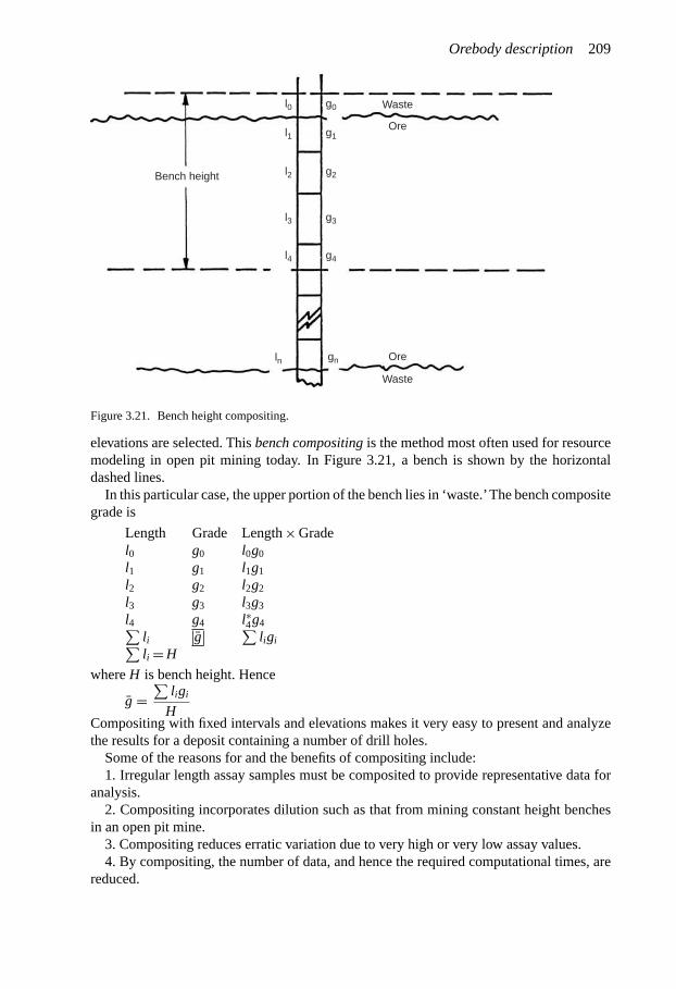
Orebody description
Bench height
l0 g0
g1
g2
g3
g4
gn
l1
l2
l3
l4
ln Ore
Waste
Waste
Ore
Figure 3.21. Bench height compositing.
elevations are selected. This bench compositing is the method most often used for resourcemodeling in open pit mining today. In Figure 3.21, a bench is shown by the horizontaldashed lines.
In this particular case, the upper portion of the bench lies in ‘waste.’The bench compositegrade is
Length Grade Length × Gradel0 g0 l0g0
l1 g1 l1g1
l2 g2 l2g2
l3 g3 l3g3
l4 g4 l∗4g4∑li g
∑ligi∑
li = H
where H is bench height. Hence
g =∑
ligi
HCompositing with fixed intervals and elevations makes it very easy to present and analyzethe results for a deposit containing a number of drill holes.
Some of the reasons for and the benefits of compositing include:1. Irregular length assay samples must be composited to provide representative data for
analysis.2. Compositing incorporates dilution such as that from mining constant height benches
in an open pit mine.3. Compositing reduces erratic variation due to very high or very low assay values.4. By compositing, the number of data, and hence the required computational times, are
reduced.
209

Open pit mine planning and design: Fundamentals
Table 3.8. Example of drill-hole log, after (Davey, 1979).
Drill-hole ID = C-22Collar location = 1800.0 N 800.0 EElevation = 45198.0Azimuth = 0.0 Attitude = −90
Depth Assay
5 0.40010 0.56015 0.44020 0.48025 0.40030 0.38035 0.33040 0.59045 0.48050 0.60055 0.56060 0.32065 0.70070 0.21075 0.18080 0.08085 0.20090 0.070
To illustrate the principles presented, consider the simplified drill hole log (Davey, 1979)given in Table 3.8.
It has been decided that 40 ft high benches and a 5200 ft reference elevation will be used.This means that bench crest elevations would be at 5200 ft, 5160 ft, 5120 ft, etc. The upper38 ft of hole C-22 would lie in bench 1. The next 40 ft would be in bench 2 and the holewould terminate in bench 3. Using the procedure outlined above, the composite grade atthis hole location for bench 2 is determined as:
Length (ft) Grade (%) Length × Grade (ft%)2 0.590 1.185 0.480 2.405 0.600 3.005 0.560 2.805 0.320 1.605 0.700 3.505 0.210 1.055 0.180 0.903 0.080 0.24
40 0.417 16.67
g = 16.67
40= 0.417
210

Orebody description
The mid-elevation of the bench 2 is 5140.0 ft. Composites of the remaining portions of thedrill hole lying above and below this bench may be found in the same way. The results aregiven below.
Bench Center coordinates Grade
E N Elevation
1 800.00 1800.00 5179.00 0.4402 800.00 1800.00 5140.00 0.4173 800.00 1800.00 5114.00 0.126
If material running 0.3% and higher is understood to be ore, then the ore-zone at this holeextends from the surface to a depth of 65 ft. The ore-zone composite would be:
Length (ft) Grade (%) Length × Grade (ft%)5 0.40 2.005 0.56 2.805 0.44 2.205 0.48 2.405 0.40 2.005 0.38 1.905 0.33 1.655 0.59 2.955 0.48 2.405 0.60 3.005 0.56 2.805 0.32 1.605 0.70 3.50
65 0.48 31.20
g = 31.2
65= 0.48
In this case when the lengths are all equal, the average grade is just the simple average ofthe grades.
g = 6.24
13= 0.48
The same compositing technique can be used when dealing with grades representing differentareas or volumes. This will be demonstrated in Section 3.5.
3.4.2 Tonnage factors
In mining, although volumes of material are removed, payment is normally received on thebasis of the weight of the valuable material contained. This is in contrast to civil construc-tion projects where normally payment is received based simply upon the material volumeremoved or emplaced. Even here, however, the conversion from volume to weight must
211

Open pit mine planning and design: Fundamentals
often be made due to the lifting and carrying limitations of the loading and hauling equip-ment used. The conversion from volume V to weight W and vice versa is done in the Englishsystem of units with the help of a tonnage factor TF (volume/weight):
V = TF × W (3.4)
where TF is the tonnage factor (volume/weight), V is the volume, and W is the weight. Thedetermination of a representative factor(s) is quite important to mining operations.
In the English system of measurement, the basic unit for describing the weight of materialsis the weight of a cubic foot of water. The density WD of water is
WD(H2O) = 62.4 lb/ft3 (3.5)
and its specific gravity SG is 1. If the mined material has a specific gravity of 2.5, its weightdensity is
WD = SG × WD(H2O) = 2.5 × 62.4 lb/ft3 = 156 lb/ft3 (3.6)
The tonnage factor TF for the material (assuming that the short ton (st) applies) is
TF = 2000 lb/st
156 lb/ft3= 12.82 ft3/st (3.7)
In the metric system, the density of water is
WD(H2O) = 1 g/cm3 = 1000 kg/m3 = 1 t/m3 (3.8)
Since the specific gravity of the mined material is 2.5, the density is 2.5 t/m3. The tonnagefactor is
TF = 1
2.5= 0.4 m3/t (3.9)
Although the tonnage factor as defined here with units of volume per weight is probably themost commonly used, the inverse (TF*) is also used:
TF∗ = W
V
Other units such as yd3 instead of ft3 are sometimes used for convenience.Although simple in principle, it is not as easy in practice to determine the appropriate
material densities to be used in the calculations. There can be many different materialsinvolved in an open pit mine and each ‘material’ can vary in density from point to point.
Three techniques are available for determining material density:1. Density testing of small samples in the laboratory.2. Careful excavation and weighing of a large volume.3. Calculation based upon composition (mineralogy) using published densities such as
given in Tables 3.9 through 3.11.Depending upon the requirements, all three are sometimes used. For Technique 1, there
are two primary tests which are done. In the first, the sample is first weighed (W ) in air. Thesample volume V is then determined by water displacement (the water level in a graduatedcylinder is, for example, compared before immersion and after immersion of the sample).
212

Orebody description
Table 3.9. Average density of minerals (Westerfelt, 1961).
Material Mineral Density Material Mineral Density(g/cm3) (g/cm3)
Antimony Native 6.7 Iron Arsenopyrite 6.0Stibnite 4.6 (continued) Hematite 5.0
Arsenic Orpiment 3.5 Magnetite 5.0Realgar 3.5 Limonite 3.8
Barium Barite 4.5 Siderite 3.8Witherite 4.3 Lead Galena 7.5
Calcium Calcite 2.7 Cerussite 6.5Aragonite 3.0 Anglesite 6.3Gypsum 2.3 Crocoite 6.0Fluorspar 3.2 Pyromorphite 7.0Apatite 3.2 Manganese Pyrolusite 4.8
Coal Anthracite 1.5 Psilomelane 4.2Bituminous 1.3 Rhodochrosite 3.6
Cobalt Linnaite 4.9 Rhodonite 3.6Smaltite 6.5 Mercury Native 14.4Cobaltite 6.2 Cinnabar 8.1Erythrite 3.0 Molybdenum Molybdenite 4.7
Copper Native 8.9 Nickel Millenite 5.6Chalcocite 5.7 Niccolite 7.5Chalcopyrite 4.2 Platinum Native 17.5Bornite 5.0 Silver Native 10.5Enargite 4.4 Argentite 7.3Tetrahedrite 4.9 Sylvanite 8.0Atacamite 3.8 Pyrargyrite 5.8Cuprite 6.0 Cerargyrite 5.4Chalcanthite 2.2 Sulphur Native 2.1Malachite 3.9 Tin Cassiterite 6.8Azurite 3.7 Stannite 4.5Chrysocolla 2.2 Tungsten Wolframite 7.3Dioptase 3.3 Scheelite 6.0
Gold Native 19.0 Zinc Blende 4.0Iron Pyrite 5.1 Zincite 5.7
Marcasite 4.8 Smithsonite 4.4Pyrrhotite 4.6
The density d is then calculated:
d = W
V(3.10)
In the second type of test, the sample is first weighed (W ) in air and then weighed (S) whensuspended in water. The specific gravity is
SG = W
W − S(3.11)
Care must be taken to correct both for porosity and moisture.Technique 2 is the most expensive and time consuming, but provides the best site specific
results. Such tests would have to be made for different locations in the mine.
213

Open pit mine planning and design: Fundamentals
Table 3.10. Average density of some common rock types (Reich, 1961).
Origin Rock type Density Origin Rock type Density(g/cm3) (g/cm3)
1. Igneous Nepheline syenite 2.62 3. Metamorphic Phyllite 2.74(plutonic) Granite 2.65 (continued) Marble 2.78
Quartz 2.65 Chlorite schist 2.87Anorthosite 2.73 Serpentine 2.95Syenite 2.74 4. Sedimentary Greywacke 2.69Quartz diorite 2.79 (consolidated) Sandstone 2.65Diorite 2.93 Limestone 2.73Gabbro 3.00 Argillaceous shale 2.78Peridotite 3.06 Calcareous shale 2.67Pyroxene 3.22 Chert 2.76
2. Igneous Quartz porphyry 2.63 5. Sedimentary Humus soil 1.45(hypabasal/ Porphyry 2.67 (unconsolidated) Surface soil 1.73volcanic) Diabase 2.94 Clayey sand/sandy 1.93
Rhyolite 2.50 Gravel, very damp 2.00Phonolite 2.56 Dry, loose soil 1.13Trachyte 2.58 Very fine, sandy 1.33Dacite 2.59 alluvium 1.51Andesite 2.62 Carbonaceous loam 1.65Basalt 2.90 Glayey, sandy soil 2.25
3. Metamorphic Orthoclase gneiss 2.70 Very wet, quartzPlagioclase gneiss 2.84 sandQuartz schist 2.68 Loess 2.64Mica schist 2.73 Clay 2.58
Table 3.11. Density of some metals (CRC Handbookof Chemistry and Physics, 1991–1992).
Metal Density(g/cm3)
Chromium 6.92Copper 8.89Gold 19.3Iron 7.86Lead 11.34Molybdenum 9.0Nickel 8.6Platinum 21.37Silver 10.5Zinc 7.13
To illustrate the use of Technique 3, consider a gold ore made up of 94% quartz and6% iron pyrite by weight. From Tables 3.9 and 3.10 one finds that the respective specificgravities are:
– Quartz: 2.65– Iron pyrite: 5.1
214

Orebody description
The overall specific gravity for the ore is
SG = 2.65 × 0.94 + 5.1 × 0.06 = 2.80
and the tonnage factor (English system) is
TF = 2000
2.80 × 62.4= 11.45 ft3/st
A margin of safety is introduced when applying the results of any of the techniques. In thiscase a value of 12 or even greater might be used. This is the in-situ or in-place tonnage factor.
To illustrate the principles involved in the conversion from volumes to weight and viceversa assume that a mining company has a contract to sell 5000 tons of metal X per year.The mined material contains 1% of the contained metal and the processing plant recovers50%. The total tonnage TA which must be mined and processed each year is given by
TA = 5000 st
0.01 × 0.50= 1, 000, 000 st
Assuming that the layer being mined has a thickness t of 20 ft, the question becomes howlarge a plan area A must be exposed to produce the required tonnage.
The annual volume VA is
VA = tA
To solve the problem, the relationship between the volume VA and the weight TA must beknown. Assuming that the specific gravity of the mined material is 2.5, the tonnage factoris 12.82 ft3/st.
Hence, the volume removed per year is
VA = 12.82 ft3/st × 1, 000, 000 st = 12, 820, 000 ft3
Hence, the area to be exposed is
A = 12, 820, 000
20= 641, 000 ft2
The acre is commonly used to describe land area:
1 acre = 43, 560 ft2
Thus, a total of 14.72 acres would be mined each year.The same problem will now be worked using the metric system. It is assumed that 4537 t
of mineral are produced from a seam 6.1 m thick. The numerical value of the density andthe specific gravity are the same in this system, which simplifies the calculations.
Since the specific gravity of the mined material is 2.5, the density is 2.5 t/m3. The tonnagefactor is
TF = 1
2.5= 0.4 m3/t
Therefore
VA = 4, 537
0.5 × 0.01× 0.4 = 362, 960 m3
A = 59, 502 m2
215

Open pit mine planning and design: Fundamentals
In the metric system, land area is expressed in terms of the hectare:
1 hectare = 100 m × 100 m = 10, 000 m2
Thus a total of 5.95 hectares would be mined each year.
3.5 METHOD OF VERTICAL SECTIONS
3.5.1 Introduction
The traditional method for estimating ore reserves has been through the use of sections. Themethod has a number of advantages, the primary one is that it can be done by hand. Otheradvantages are that it can be easily depicted, understood and checked. It will be assumedthat the method is done by hand. However, a number of computer techniques are availableto allow designer input/flexibility while doing the calculations by machine. Some computerprograms have been designed to essentially reproduce the interpretation logic currently doneby engineers and geologists by hand.
3.5.2 Procedures
The general procedures described below have been used by the Office of Ore Estimation-University of Minnesota (Weaton, 1972, 1973) for preparing and/or reviewing iron orereserve estimates for the State of Minnesota. They can easily be adapted to other types ofmineralization and deposits.
Planning materials1. A current, up-to-date plan map. This is made to a convenient scale (usually 1 in = 100 ft)and shows the following:
(a) Pit surface conditions, existing banks and details of the immediate vicinity.(b) Location of all drill holes.(c) Location of all quarter section lines and property lines.(d) Location of pit cross sections.
2. A complete set of cross sections. These are drawn to any convenient scale (usually 40feet to the inch) and contain the following:
(a) All exploration drill holes which fall on or close to the section (half way to the nextsection), with the detailed analysis of each sample taken. Results of hand wash or heavydensity tests if they were made. Also, the location and analysis of any bank samples thathave been taken.
(b) A line showing the current top of the material remaining in the ground undisturbed.(c) Geologic structure lines showing an interpretation of the limits of the ore areas, and
the various lean ore (low grade) or waste formations.
Planning procedures1. Drill samples are evaluated on the cross sections and zones of different types of material arecolor coded for convenience. If the pit has been operating, any pit operations or observationswhich may disprove drilling samples in any way are taken into consideration in outliningzones of the various types of materials.
216

Orebody description
2. Limits of ore materials are transposed to the plan map as a general outline for the pitarea.
3. The pit plan layout is developed to recover all of the ore that is economically minablewith the necessary removal of the waste materials. Many factors enter into this plan, andgovern the amount of material which must be removed. Some of these are:
(a) The nature of the surface capping; i.e., sand, clay, gravel, muskeg, etc., and the angleat which this material will remain stable in the bank.
(b) The nature of the rock and waste material and the angle at which it will remain stablewhen exposed.
(c) The local terrain and the location of the mine facilities, plant and dump areas in relationto the pit.
(d) The grade or steepness of the haulage road and the width required by the haulagetrucks.
(e) The number of berms or protective benches that will be required to insure pit safetyand bank stability.
4. After the pit plan is laid out, and the bank slopes are drawn on the cross sections, tonnagescan be computed.
5. Unless disproven by other drilling or samplings, the material on each cross section isassumed to extend to a point one half the distance to the section on each side or 100 feetbeyond the end section.
6. Computation of volumes in cubic feet are made by measuring the area of each type ofmaterial as shown on the cross section, and multiplying this by the distance represented bythe section (one-half the distance to each adjacent section). By experience, the factor ofcubic feet per ton has been established, for both ore and other materials. Concentration testson drill samples of materials requiring plant treatment establish the recovery figure or howmuch concentrate will remain after being run through a concentration plant.
7. Tonnages of each section are totalled to give the final reserve tonnage figures.
8. A weighted average of the chemical analyses of each type of material is computed toproduce the final estimated grade of the products included in the estimate.
3.5.3 Construction of a cross-section
An E-W section (640 N) taken through an iron deposit is shown in Figure 3.22. The objectiveis to begin with the drill hole data and proceed through to the determination of the areas ofthe different materials which would be included in the final pit. The symbols which havebeen used to denote the layers are:
SU = surface (overburden) material (soil, glacial till, etc.) which can be removed withoutdrilling and blasting.
DT = decomposed taconite.OP = ore and paint rock.OT = ore and taconite.SWT = sandy wash ore and taconite.
217

218 Open pit mine planning and design: Fundamentals
SECTION 640 N
DDH 6 DDH 57 DDH 60
SUSU SU
DT DT
DT
OT
HM
SW
LO
OP OP
OP OPOT
LO LOOT OT
ODT ODT
OT
SWT SWTBES BES
Elevation
1500
1450
1400
1350
1300
1250
100E 200E 300E 400E 500E 600E 700E 800E 900E 1000E
Figure 3.22. Drill holes and topography added to the section (Step 1).
BES = Bessemer ore.ODT = ore and decomposed taconite.LO = lean (low grade) ore.SW = sandy wash ore.HM = heavy media ore.Step 1. The drill holes and surface topography are plotted on the section.Step 2. The bisector between DDH57 and DDH60 is constructed. The surface-rock
interface is drawn. Points common to all 3 holes are connected (Fig. 3.23).Step 3. Starting from the surface, connect the remaining common points in holes DDH57
and DDH6 and extend them to the left of DDH6. To the right of DDH57 extend the layersover to the bisector line. These are drawn parallel to the known overlying surfaces. Fill inthe region between DDH57 and the bisector by extending the layers parallel to the knownoverlying trend lines. (Fig. 3.24).
Step 4. The remaining layers intersected by DDH60 are extended left to the bisector andto the right. (Fig. 3.25).
Step 5. The pit outline is superimposed on the section. In this case the following ruleshave been used:
– the lean ore intercept forms the pit bottom,– an extension of 50 ft outside of the drill holes at the pit bottom is assumed,– the allowable pit slope angle in the surface material is 27◦ whereas in the rock layers
near the pit bottom it is 54◦. A transition of 41◦ is used between these. (Fig. 3.26).Step 6. An access road 50 ft in width crosses this section at the position indicated
(Fig. 3.27).

Orebody description 219
SECTION 640 N
DDH 6 DDH 57 DDH 60
SU SUSU
DT DT
DT
OP OPOT OT
OT
OP OPSWT SWT
SW
BES BES
ODT ODTOT OTLO LO
LO
HM
Elevation
1500
1450
1400
1350
1300
1250
1000E900E800E700E600E500E400E200E 300E100E
Bisector
Figure 3.23. The Step 2 section.
SECTION 640 N
DDH 6 DDH 57 DDH 60
SUSU SU
DT DT
DT
OT
HM
SW
LO
OP OP
OP OPOT
LO LOOT OTODT ODT
OT
SWT SWTBES BES
Elevation
1500
1450
1400
1350
1300
1250
100E 200E 300E 400E 500E 600E 700E 800E 900E 1000E
Bisector
Figure 3.24. The Step 3 section.

220 Open pit mine planning and design: Fundamentals
SECTION 640 N
DDH 6 DDH 57 DDH 60
SUSU SU
DT DT
DT
OT
HM
SW
LO
OP OP
OP OPOT
LO LOOT OTODT ODT
OT
SWT SWTBES BES
Elevation
1500
1450
1400
1350
1300
1250
100E 200E 300E 400E 500E 600E 700E 800E 900E 1000E
Bisector
Figure 3.25. The Step 4 section.
DDH 6 DDH 57 DDH 60
SUSU SU
DT DTDT
OT
HM
SW
LO
OP OP
OP OPOT
LO LOOT OT
ODT ODT
OT
SWT SWTBES BES
Elevation
1500
1450
1400
1350
1300
1250
100E 200E 300E 400E 500E 600E 700E 800E 900E 1000E
27°
27°
41°41°
54°54°
50°50°
SECTION 640 N
Figure 3.26. The Step 5 section.

Orebody description 221
DDH 6 DDH 57 DDH 60
SUSU SU
DT DT
DT
OT
HM
SW
LO
OP OP
OP OPOT
LO LOOT OTODT ODT
OT
SWT SWTBES BES
Elevation
1500
1450
1400
1350
1300
1250
100E 200E 300E 400E 500E 600E 700E 800E 900E 1000E
Road
cut
SECTION 640 N
Figure 3.27. The Step 6 section.
Step 7. The areas of the different materials on the section are determined using aplanimeter (Fig. 3.28).
Even in this relatively simple case, it is clear that a good knowledge of the structureof the orebody is required (Fig. 3.29) as well as some judgement in order to create suchsections. As will be discussed in more detail later, final pit outlines can only be determinedby considering all sections together.
3.5.4 Calculation of tonnage and average grade for a pit
This simplified example has also been taken from iron mining practice. The followingconcepts will be illustrated:
1. Side completion for sections.2. Development of a final pit outline including pit ends.3. Determination of tons and average grade for a section.4. Determination of tons and average grade for the pit.
Although most of the discussion will revolve around section 1 + 00, the same approachwould be used on all sections.
Side completionAs described in the previous example, the section 1 + 00 (Fig. 3.30) has been extended50 ft past the positions of the outermost drill holes. On the left side of the section, the oreappears to pinch out within this zone. The pit slope of 27◦ has been drawn to pass throughthe mid-height of this extension. The width associated with hole 6 would be 50 ft plus halfthe distance between holes 6 and 1. On the right-hand side, the ore is quite thick (25 ft) and

222 Open pit mine planning and design: Fundamentals
Elevation
1500
1450
1400
1350
1300
1250
100E 200E 300E 400E 500E 600E 700E 800E 900E 1000E
SECTION 640 N
SURFACE (12.48 in2)
Ore and Taconite (3.42 in2)Ore and Paint Rock
Ore and Decomposed Taconite
Ore and Taconite(0.28 in2)
(0.43 in2)(0.27 in2)
Sandy Wash Taconite(0.16 in2)
(0.55 in2)
Decomposed Taconite(1.15 in2)
Bessemer Ore
(1.23 in2)
Heavy Media Ore (0.84 in2)
Sandy Wash Ore(1.92 in2)
Figure 3.28. The Step 7 (final) section.
ALTERNATELIMIT NO.2 ALTERNATE LIMIT NO.1
ALTERNATE LIMIT NO.3ALTERNATELIMIT NO.4
Figure 3.29. A typical cross section showing the structure of a Minnesota Mesabi range iron orebody(Axelson, 1963).
would appear to continue. The slope has been drawn at a point measured 50 ft along the pitbottom. The ore width associated with hole 5 becomes 75 ft.
Final pit outlineThe surface is assumed to be flat and at 0 elevation. A bench height of 25 will be used.Through an examination of all sections, it is seen that the overburden-rock interface lies atan average elevation of about 100 ft. In the plan view shown in Figure 3.31, the surface (×)and 100 ft intercepts (◦) read from the 6 sections have been marked.

Orebody description
223
300N 400N 500N 600N 700N 800N 900N 1000N 1100N 200
150
100
50
0
Elevation With Respectto the Surface
SECTION 1�00
DDH 6 DDH 1 DDH 2 DDH 3 DDH 4 DDH 5
50' 50' 100' 100' 50' 150' 75'
27° Taconite
5112053
61585450
52545958
14050'
6161
60
58
5157
160
63 55 57
58
55
150
135
535857
60536055
62
50
59
62
Taconite � 1.80 in2
Ore � 4.15 in2
Surface � 15.16 in2
50'
52
5855
125
27°
Figure 3.30. Section used for the average sectional grade and tonnage calculation.

224 Open pit mine planning and design: Fundamentals
200N
300N
400N
500N
600N
700N
800N
900N
1000N
1100N
1200N
1300N1�00 4�00 6�00 8�00 11�00 13�00
5
43
2
16
Figure 3.31. Plan smoothing of the pit limits.
The ends of the pit must now be completed. There are several possible constructionswhich might be used.
1. Construct longitudinal sections through the orebody and estimate ore continuation byprojection.
2. Extend the ore a distance equal to the ore thickness observed in the end section.3. Extend the ends some fixed distance past the last section. For example 100 ft or a
distance equal to half the distance between sections.In this particular case, the second method was selected. As can be seen in Figure 3.30, the
maximum ore thickness of 60 ft occurs in hole 2. This thickness extends in plan from holes1 to 4. Projection of the lines from the pit bottom to the 100 ft and surface elevations yieldsthe points a, b, c and d shown on Figure 3.32. The same procedure has been followed onthe east end of the pit where the ore thickness is 40 ft. The final step is to connect the pointsby smooth curves. In this case, the transition between sections is smooth and no furtheradjustment is required. If the individual sections do not fit together as nicely as in Figure3.32, then obviously an iterative procedure of going from plan to section to plan, etc. isrequired.
Tonnage and average grade for a sectionSection 1 + 00 is defined by 6 drillholes. The first step in determining average grade for thesection is to find the average grade for each drill hole. If the sample interval was always thesame then a simple average of the assays would suffice. In general this is not the case andcompositing must be done. The results of this are given in Table 3.12. An influence area foreach hole must now be calculated. This area is the ore intercept height times a width. Forinterior holes, the width extends halfway to adjacent holes. For side holes the width extends

Orebody description 225
1�00 4�00 6�00 8�00 11�00 13�00
1300N
1200N
1100N
1000N
900N
800N
700N
600N
500N
400N
300N
200N
16
2
34
5 100' Elevation
ab
c d
196'
196'
Figure 3.32. Addition of pit ends.
from the side line halfway to the adjacent hole. For this section, the influence areas are asshown in Figure 3.33 and summarized in Table 3.13. Using the grades and influence areas,an average grade for the section is determined by compositing. In this case it is 56.8% Fe.
Tons and average grade for the pitThe ore volume attributed to the section is obtained by multiplying the section area (deter-mined by calculation or planimeter) by the section interval which for section 1 + 00 is 210 ft(Table 3.14). For this section the ore volume is 4,357,500 ft3. Applying a tonnage factor of14 ft3/lt yields 311,000 tons.
Similar figures are developed for each of the other sections. The average grade for the pitis obtained by compositing. The total ore tonnage is just the sum of the tons (A).
The associated waste consists of two types:– surface material, and– taconite.On each section, the areas of each material type are determined by planimetering. The
results for section 1 + 00 are given in Tables 3.15 and 3.16.
Pit end tonnageA somewhat troublesome problem is deciding how to include the material making up thepit ends. The west end of the pit will be examined in this example assuming that all ofthe material above the 100 ft contour is surface material. In Figure 3.33, the end has beendivided into five sectors which will be approximated by the following two shapes.
– prism (A1), and– frustum of a right cone (A2 →A5).

226 Open pit mine planning and design: Fundamentals
Table 3.12. Calculating average hole analyses (Pfleider, 1962).
Cross-sect. DH From To Length Avg Analysis-dry Length ×Analysis(ft) (Fe%) (ft × %Fe)
1 + 00 1 100 105 5 58 290105 110 5 61 305110 115 5 59 295115 120 5 58 290120 125 5 54 270125 130 5 54 270130 135 5 52 260135 140 5 50 250
Avg 100 140 40 55.8 22302 100 105 5 61 305
105 110 5 63 315110 115 5 61 305115 120 5 59 295120 130 10 60 600130 140 10 62 620140 150 10 58 580150 155 5 57 285155 160 5 51 255
Avg 100 160 60 59.3 35603 100 105 5 57 285
105 110 5 55 275110 120 10 58 580120 130 10 62 620130 140 10 55 550140 150 10 50 500
Avg 100 150 50 56.2 28104 100 105 5 60 300
105 110 5 57 285110 115 5 53 265115 120 5 58 290120 125 5 60 300125 130 5 53 265130 135 5 55 275
Avg 100 135 35 56.6 19805 100 110 10 58 580
110 120 10 55 550120 125 5 52 260
Avg 100 125 25 55.6 13906 110 115 5 53 265
115 120 5 51 255
Avg 110 120 10 52.0 520
An isometric drawing of sectors A1, A2 and A3 is shown in Figure 3.34. The individualparts are shown in Figure 3.35. The general formula for the volume of a prism is
Vp = 1
2(S1 + S2)h (3.12)

Orebody description 227
1�00 4�00 6�00 8�00 11�00 13�001300N
1200N
1100N
1000N
900N
800N
700N
600N
500N
400N
300N
200N
140'
250'250'250' 200'210'
40'
60'
45°
45°
Sector Line
Secto
r Lin
e
ab
c L
c L
cL
cL
1
6
2
3
4
5
dc
A1
A4
A5
A2
A3
60'
Figure 3.33. Pit end volume calculations.
Table 3.13. Calculating average section analyses (Pfleider, 1962).
Cross-sect. Hole From To Length Dist. bet Area Avg Analysis Area × %No. holes (ft2) (%Fe) (ft2 × %Fe)
1 + 00 1 100 140 40 75 3,000 55.8 167,4002 100 160 60 100 6,000 59.3 355,8003 100 150 50 75 3,750 56.2 210,7504 100 135 35 100 3,500 56.6 198,1005 100 125 25 150 3,750 55.6 208,5006 110 120 100 75 750 52.0 39,000
Total 20,750 56.8 1,180,000
where S1, S2 are the areas of the top and bottom surfaces, respectively, and h is the altitude.The formula for the volume of a right cone is
Vc = 1
3πr2h (3.13)
where r is the radius of the base.The formula for the volume of the frustum of a right cone is
Vfc = πh
3(r2
1 + r1r2 + r22 ) (3.14)
where r1 is the radius of the base and r2 is the radius of the top.

228 Open pit mine planning and design: Fundamentals
Table 3.14. Summary sheet for ore tons and grade (Pfleider, 1962).
Cross- Planimetered Area Section Section Volume Tonnage Tons Grade Tons × %sect. area (in2) factor area interval (ft3) factor (lt) (%) (lt × %Fe)
(ft2/in2) (ft2) (ft) (ft3/lt) (%Fe)
1 + 00 4.15 50 × 100 20,750 210 4,357,500 14 311,000 56.8 17,664,8004 + 00 2506 + 00 2008 + 00 250
11 + 00 25013 + 00 140
Grand total AB
AB
Table 3.15. Summary sheet for surface material (Pfleider, 1962).
Cross- Planimetered Area factor Section Section Volume Volume Tonnage Tonssect. area (in2) (ft2/in2) area interval (ft3) (yd3) factor (st)
(ft2) (ft) (ft3/st)
1 + 00 15.16 50 × 100 75,800 210 15,918,000 590,000 19 838,0004 + 006 + 008 + 00
11 + 0013 + 00
Total A B
Table 3.16. Summary sheet for taconite (Pfleider, 1962).
Cross-sect. Plan. area Area factor Section Section Volume Tonnage Tons(in2) (ft2/in2) area interval (ft3) factor (st)
(ft2) (ft) (ft3/st)
1 + 004 + 006 + 008 + 00
11 + 0013 + 00
Total C
Applying formula (3.12) to sector A1, one finds
VA1 = 1
2(60 × 240 + 256 × 240)100 = 3, 792, 000 ft3
For sector A2, base and top radii are determined along the sector centerlines. These become:
r1 = 293 ft
r2 = 60 ft

Orebody description 229
A1
A2
A3
Figure 3.34. Isometric view of sections A1, A2 and A3.
A1
240'
100'
27°
60'
Axis ofrevolution
Axis ofrevolution
A2
A3r3
r4r2
r1
θ2
θ1
Figure 3.35. Exploded view of the pit end volumes.

230 Open pit mine planning and design: Fundamentals
The included angle (θ) of the sector is 45◦. Hence
VA2 = π
3100(2932 + 293 × 60 + 602)
45
360= 1, 401, 010 ft3
For sector A3:
θ2 = 45◦
r3 = 387 ft
r4 = 93 ft
VA3 = π
3100(3872 + 387 × 93 + 932)
45
360= 2, 544, 814 ft3
Similarly for sectors A4 and A5:
VA4 = π
3100(2932 + 293 × 53 + 532)
45
360= 1, 363, 808 ft3
VA5 = π
3100(3462 + 346 × 93 + 932)
45
360= 2, 101, 508 ft3
The total volume of the west end then becomes
Vwe = 11, 204, 000 ft3
Applying a tonnage factor of 19 ft3/st, yields 590,000 st. The split between taconite and rockcan be found by including the interface in the drawings.
In estimating actual grade and tonnage from the pit one must take into account:– ore losses in pit,– dilution, and– mill recovery.
3.6 METHOD OF VERTICAL SECTIONS (GRADE CONTOURS)
A less commonly used technique to represent grades on sections is through iso-grade con-tours. Although there are several reasons for adopting such an approach, the primary onein the example to be considered is the fact that the directions of the exploratory drill holeswere highly variable. This example, using the data and approach of Cherrier (1968), willdemonstrate the application of the technique for determining tons and average grade andalso the application of longitudinal sections for completing pit ends. Figure 3.36 is a planmap for a molybdenum orebody showing the location of the drill holes and the surfacetopography. The grid system has been superimposed. Sections 4, 8, 12, 16 and 20 are givenin Figures 3.37 through 3.41. The drill holes on Sections 2 and 22 revealed no ore present.Using the drill hole data and a knowledge of the deposit form, the grade contours havebeen created. A pit outline has been developed using procedures which will be describedin Chapter 5. In viewing the 5 transverse sections, it can be seen that longitudinal section3200 N runs approximately along the proposed pit axis. This section is shown in Figure3.42. Rock mechanics studies have suggested a 45◦ slope angle at the east end and 50◦ atthe west. From the drilling results, the orebody must terminate between Sections 2 to 4 onthe west and 20 to 22 on the east. The grade contour lines have been drawn in to representthis (Fig. 3.43) condition. In examining the plan representation (Fig. 3.44) of the final pit,

Orebody description 231
Figure 3.36. Plan map showing drill hole locations (Cherrier, 1968).
Elevation
12200
12000
11800
11600
11400
11200
11000
2600N 2800N 3000N 3200N 3400N 3600N 3800N 4000N
SECTION 4
Pit Outline
Surface
DDH 19DDH 1
DDH 20
0.3
0.12
0.2
Figure 3.37. Section 4 showing the grade contours and pit outline (Cherrier, 1968).

232 Open pit mine planning and design: Fundamentals
Elevation
12600
12400
12200
12000
11800
11600
11400
2600N 2800N 3000N 3200N 3400N 3600N 3800N 4000N
SECTION 8
Pit Outline
DDH 5
DDH 23
DDH 4DDH 22 Surface
0.2
0.3
0.12
Figure 3.38. Section 8 showing the grade contours and pit outline (Cherrier, 1968).
Elevation
12600
12400
12200
12000
11800
11600
11400
2600N 2800N 3000N 3200N 3400N 3600N 3800N 4000N
SECTION 12
Pit Outline
DDH 27
DDH 26
DDH 8
DDH 25
0.3
0.20.12
Surface
Figure 3.39. Section 12 showing the grade contours and pit outline (Cherrier, 1968).

Orebody description 233
Elevation
12800
12600
12400
12200
12000
11800
11600
2600N 2800N 3000N 3200N 3400N 3600N 3800N 4000N
DDH 12
DDH 31
DDH 30
Surface
0.12
0.20.3
SECTION 16
Pit Outline
Figure 3.40. Section 16 showing the grade contours and pit outline (Cherrier, 1968).
Elevation
12600
12400
12200
12000
11800
11600
11400
2600N 2800N 3000N 3200N 3400N 3600N 3800N2400N
SECTION 20
Pit Outline
DDH 36
DD
H 15
DD
H 14
DDH 35
0.12
0.2 0.3
Surface
Figure 3.41. Section 20 showing the grade contours and pit outline (Cherrier, 1968).

234 Open pit mine planning and design: Fundamentals
11400
11600
11800
12000
12200
12400
12600
Elevation SECTION 3200 N
0 2 4 6 8 10 12 14 16 18 20 22 24 26 28Section
50°
45°0.2
0.3
0.12
Pit Outline
Figure 3.42. Longitudinal Section 3200 N showing the grade contours, surface topography and pit outline(Cherrier, 1968).
Elevation
12600
12400
12200
12000
11800
11600
11400
Influence ofSection 4
SECTION 3200 N Influence of Section 20
0 2 4 6 8 10 12 14 16 18 20 22 24 26 28
Section
0.2
0.3
0.12
Pit Outline
Figure 3.43. Grade contours completed at the pit ends.
and the longitudinal section, it has been decided to incorporate the end volumes of the pitinto Sections 4 and 20 rather than to treat them separately. This is accomplished by varyingthe longitudinal length of influence so that the resulting volumes are correct. For the eastand west ends the following have been used:
Section 4 Grade zone Influence distance (ft)+0.3 200
0.2−0.3 2250.12−0.2 250Overburden 300

Orebody description 235
0 2 4 6 8 10 12 14 16 18 20 22 24 26 28
Section
2400N
2600N
2800N
3000N
3200N
3400N
3600N
3800N
4000NInfluenceSection 4
Influence Section 20
Figure 3.44. Plan view showing outline of pit crest and toe.
20 +0.3 2000.2−0.3 250
0.12−0.2 300Overburden 400
The reader is encouraged to check these approximations. For each section the areascorresponding to each grade zone within the pit outline are determined using a planimeter.These are then converted into volumes and tons as summarized in Table 3.17. A summaryof ore and waste tons as well as the ratio of the two (average stripping ratio) by section isgiven in Table 3.18. The overall stripping ratio for the pit is also calculated.
One assay was performed for each 10 ft of core in every drill hole. For each section, theassays lying within a particular grade zone were added together. This sum was then dividedby the number of assays to obtain an average. Each average assay was weighted by thevolume of influence for the respective zone. These weighted averages were totalled anddivided by the total volume for the three zones. This figure is then the average assay for theentire ore zone on that section. The results of this calculation are given in Table 3.19. Theoverall average grade for the pit is found in Table 3.20.
In summary:
Tonnage of ore = 53,288,000 stAverage grade = 0.281 percent (MoS2)Tonnage of overburden = 32,311,000 stAverage stripping ratio = 0.61
Some dilution and ore loss can be expected from this orebody due to the difficulty of definingthe ore cut-off grade and mining to this grade in the upper half of the orebody. The followingcalculation illustrates how one might account for these effects and determine an averagegrade for the ore actually mined.

236 Open pit mine planning and design: Fundamentals
Table 3.17. Calculation of tonnage of ore and overburden (Cherrier, 1968).
Section Grade zone Area1 Influence Volume Tons2 Total tons
(in2) (104 ft2) distance (ft) (106 ft3) (×103) (×103)
4 +0.3 1.32 5.28 200 10.560.2–0.3 0.84 3.36 225 7.56 2,2660.12–0.2 1.02 4.08 250 10.20
845605816
=
Overburden 2.81 11.24 300 33.72 2,698 2,698
6 +0.3 2.52 10.08 200 20.160.2–0.3 3.46 13.84 200 27.68 5,0750.12–0.2 1.95 7.80 200 15.60
1, 6132, 2141, 248
=
Overburden 2.17 8.68 200 17.36 1,389 1,389
8 +0.3 2.97 11.88 200 23.760.12–0.3 1.66 6.64 200 13.28 3,7630.12–0.2 1.25 5.00 200 10.00
1, 9011, 062800
=
Overburden 2.62 10.48 200 20.96 1,677 1,677
10 +0.3 2.17 8.68 200 17.360.2–0.3 3.00 12.00 200 24.00 4,4230.12–0.2 1.74 6.96 200 13.92
1, 3891, 9201, 114
=
Overburden 5.66 22.64 200 45.28 3,622 3,622
12 +0.3 3.11 12.44 200 24.880.2–0.3 6.64 26.56 200 53.12 7,8720.12–0.3 2.55 10.20 200 20.40
1, 9904, 2501, 632
=
Overburden 3.17 12.68 200 25.36 2,029 2,029
14 +0.3 2.46 9.84 200 19.680.2–0.3 4.30 17.20 200 34.40 5,6570.12–0.2 2.08 8.32 200 16.64
1, 5742, 7521, 331
=
Overburden 6.90 27.60 200 55.20 4,416 4,416
16 +0.3 2.57 10.28 200 20.560.2–0.3 3.18 12.72 200 25.44 5,7600.12–0.2 3.25 13.00 200 26.00
1, 6452, 0352, 080
=
Overburden 5.51 22.40 200 44.08 3,526 3,526
18 +0.3 4.09 16.36 200 32.720.2–0.3 5.29 37.52 200 75.04 10,4450.12–0.2 2.85 11.40 200 22.80
2, 6186, 0031, 824
=
Overburden 6.10 24.40 200 48.80 3,904 3,904
20 +0.3 4.99 19.96 200 39.920.2–0.3 3.27 13.08 250 32.70 8,1810.12–0.2 2.47 9.88 300 29.64
3, 1942, 6162, 371
=
Overburden 7.07 28.28 400 113.12 9,050 9,050
1 Planimetered: 1 in2 = 200′ × 200′ = 40, 000 ft2.2 Based on a tonnage factor of 12.5 ft3/st.
Tons (st) Grade (%) Tons × Grade (st × %)Ore in place 53.0 × 10⁶ 0.281 14.893 × 10⁶
Dilution (est. 5%) +2.65 × 10⁶ 0.100 +0.265 × 10⁶
Ore loss (est. 5%) −2.65 × 10⁶ 0.140 −0.371 × 10⁶
Total 53.0 × 10⁶ 14.787 × 10⁶
Average grade of ore mined = 14.787
53= 0.279 percent.

Orebody description 237
Table 3.18. Calculation of the average stripping ratio.
Section Tons of ore Tons of overburden Avg stripping ratio(st × 103) (st × 103)
4 2,266 2,698 1.1916 5,075 1,389 0.2748 3,763 1,677 0.446
10 4,423 3,622 0.81912 7,872 2,029 0.25814 5,657 4,416 0.78116 5,760 3,526 0.61218 10,445 3,904 0.37420 8,181 9,050 1.106
Total 53,442 32,311
Overall average stripping ratio:32, 311
53, 442= 0.605.
3.7 THE METHOD OF HORIZONTAL SECTIONS
3.7.1 Introduction
Although vertical sections have played a dominant role in ore reserve estimation in the past,today, for many, if not most, deposits this function is rapidly being replaced by techniquesbased upon the use of horizontal sections. The primary reason being the widespread avail-ability of computers for doing the tedious, time consuming calculations involved and thedevelopment of new techniques for estimating the grades between drill holes. Sections takenin the plane of the orebody have generally been used for evaluating relatively thin, flat lyingdeposits such as uranium, coal, sand, gravel, placer gold, etc. They may be of relatively uni-form or varying thickness. Thick deposits are mined in a series of horizontal slices (benches)of uniform thickness. For extraction planning, bench plans showing tons and grade are ofutmost importance. Hence even if vertical sections are used for initial evaluation, bench(horizontal) sections are eventually required. In this section hand methods for calculatingtons and grade based on triangles and polygons will be discussed. These discussions willuse as a basis the drillholes shown in Figure 3.45. The corresponding grades and locationcoordinates are given in Table 3.21.
3.7.2 Triangles
In the triangular method, diagrammatically illustrated in Figure 3.46, each hole is taken tobe at one corner of a triangle. If the triangular solid formed is of constant thickness t, itsvolume is just equal to the plan area A times this thickness. To obtain tons, the appropriatetonnage factor is applied. The average grade g is given by
g = g1 + g2 + g3
3(3.15)
where gi are the grades at the three corners.The area of the triangle can be found using a planimeter or through calculation if the
coordinates (xi, yi) of the corners are known. This method, shown in Figure 3.47, readilyadapts to calculator/computer application. The average grade for the block is strictly correct

238 Open pit mine planning and design: Fundamentals
Table 3.19. Calculation of average assay for each section (Cherrier, 1968).
Section Grade Avg assay Volume Assay × Volume Avg assayzone (%) (×106 ft3) (% ×106 ft3) for section
4 +0.3 0.452 10.56 4.77310.2–0.3 0.270 7.56 2.04120.12–0.2 0.135 10.20 1.3770
Total 28.32 8.1913 0.289
6 +0.3 0.435 20.16 8.76960.2–0.3 0.242 27.68 6.69860.12–0.2 0.155 15.60 2.4180
Total 63.44 17.8862 0.282
8 +0.3 0.485 23.76 11.52360.2–0.3 0.246 13.28 3.26690.12–0.2 0.153 10.00 1.5300
Total 47.04 16.3205 0.347
10 +0.3 0.379 17.36 6.57940.2–0.3 0.261 24.00 6.26400.12–0.2 0.151 13.92 2.1019
Total 55.28 14.9453 0.270
12 +0.3 0.411 24.88 10.22570.2–0.3 0.243 43.12 12.90820.12–0.2 0.142 20.40 2.8968
Total 98.40 26.0307 0.265
14 +0.3 0.403 19.68 7.93100.02–0.3 0.242 34.40 8.32480.12–0.2 0.168 16.64 2.7955
Total 70.72 19.0513 0.269
16 +0.3 0.398 20.56 8.18290.2–0.3 0.247 25.44 6.28370.12–0.2 0.155 26.00 4.0300
Total 72.00 18.4966 0.257
18 +0.3 0.393 32.72 12.85900.2–0.3 0.274 75.04 20.56100.12–0.2 0.158 22.80 3.6024
Total 130.56 37.0224 0.284
20 +0.3 0.405 39.92 16.16760.2–0.3 0.261 32.70 8.53470.12–0.2 0.164 29.64 4.8610
Total 102.26 29.5633 0.289
only for equilateral triangles. For other triangle shapes the area associated with each grade isnot equal as assumed in the formula. For triangular solids which are not of constant thickness,then some additional calculations are required. The average thickness t is given by
t = t1 + t2 + t33
(3.16)
and the average grade g is
g = g1t1 + g2t2 + g3t33t
(3.17)

Orebody description 239
Table 3.20. Calculation of overall average grade (Cherrier, 1968).
Section Average Volume Assay ×Volumeassay (×106 ft3) (% × 106 ft3)
4 0.289 28.32 8.18456 0.282 63.44 17.89018 0.347 47.04 16.3229
10 0.270 55.28 14.925612 0.265 98.40 26.076014 0.269 70.72 19.023716 0.257 72.00 18.504018 0.284 130.56 37.079020 0.289 102.26 29.5531
Total 668.02 187.5589
Overall average grade of orebody:187.5589
668.02= 0.281 percent.
500E 1000E 1500E 2000E
Departure
500N
1000N
1500N
2000N
Latit
ude
Elevation 5120-5160 : Bench 5140
C-20
0.175
C-23
0.215
C-11
0.396
C-24
0.685
C-22
0.417
C-12
0.377
C-21
0.489
C-13
0.427
C-14
0.140
C-35
0.475
C-16
0.889
C-15
0.806
C-36
0.717
C-37
0.320
C-38
0.392
C-25
0.230
C-26
0.833
C-27
0.453
C-1
0.719
C-17
1.009
C-2
0.893
C-18
0.089
C-19
0.092
C-44
0.040
C-10
0.572
C-43
0.519
C-9
1.335
C-42
0.915
C-8
1.365
C-41
0.023
C-40
0.102C-7
0.644
C-39
0.476
C-51
0.228
C-47
0.165
C-32
0.228
C-4
0.188
C-33
0.027
C-34
0.225
C-5
0.395
C-50
0.012
C-49
0.996
C-48
0.406
C-31
0.063
C-28
0.409
C-46
0.258
C-3
0.638
C-37
1.615
C-6
0.765
C-30
0.465
C-45
0.034
Figure 3.45. Borehole locations and grades for Bench 5140 (Hughes & Davey, 1979).

240 Open pit mine planning and design: Fundamentals
Table 3.21. Coordinates and grades for the holes of Figure 3.45. The composite grades are for Bench 5140(Hughes & Davey, 1979).
Hole Coordinates Grade Hole Coordinates Grade(% Cu) (% Cu)
East North East North
C-1 1100 1200 0.719 C-27 900 1200 0.453C-2 1500 1200 0.893 C-28 600 700 0.409C-3 1100 800 0.638 C-29 1300 800 1.615C-4 1100 400 0.188 C-30 1700 800 0.465C-5 1500 400 0.395 C-31 1100 600 0.063C-6 1500 800 0.765 C-32 900 400 0.224C-7 500 900 0.644 C-33 1300 1400 0.027C-8 900 1000 1.365 C-34 1100 200 0.225C-9 1300 1000 1.335 C-35 1300 1400 0.475C-10 1700 1000 0.072 C-36 700 1400 0.717C-11 500 1600 0.396 C-37 500 1400 0.320C-12 900 1600 0.377 C-38 300 1400 0.392C-13 1100 1600 0.427 C-39 400 700 0.476C-14 1500 1600 0.140 C-40 400 1050 0.102C-15 900 1400 0.806 C-41 700 1000 0.023C-16 1100 1400 0.889 C-42 1100 1000 0.915C-17 1300 1200 1.009 C-43 1500 1000 0.519C-18 1700 1200 0.089 C-44 1900 1000 0.040C-19 1900 1200 0.092 C-45 1900 800 0.034C-20 600 1900 0.175 C-46 900 800 0.258C-21 1100 1800 0.489 C-47 900 600 0.165C-22 800 1800 0.417 C-48 1300 600 0.406C-23 200 1600 0.215 C-49 1500 600 0.996C-24 700 1600 0.685 C-50 1700 600 0.012C-25 500 1200 0.230 C-51 500 500 0.228C-26 800 1200 0.833
Figure 3.46. Triangular prisms (Barnes, 1979b).

Orebody description 241
(X1, Y1)
(X2, Y2)
(X3, Y3)
A1 A2
A3
A
A � (X3 �X1)(Y2 �Y1) � 1/2 (X3 �X1)(Y1 �Y3) � 1/2 (X3 �X2)(Y2 �Y3)
� 1/2 (X2 �X1)(Y2 �Y1)
A � Area of Rectangle � A1 � A2 � A3
A � (Xmax �Xmin)(Ymax �Ymin) � 1/2 (Xi �Xj)(Yi �Yj)i�1,3j�1,3
Figure 3.47. Calculation of triangular area based upon corner coordinates.
Using the average thickness, the plan area and tonnage factor, the tons can be found. Thetriangular element formed by holes C-30, C-40, and C-50 (assuming a constant benchthickness of 40 ft and a tonnage factor of 12.5 ft3/ton), contains 64,000 tons with an averagegrade 0.17.
3.7.3 Polygons
In the polygonal method, each drill hole lies within the center of a polygon. The polygon isconstructed such that its boundary is always equidistant from the nearest neighboring hole.Within the polygon, the grade is assumed constant and equal to that of the hole it includes.The thickness of the polygon is also constant and equal to the ore intercept/bench thickness.The steps followed in forming a polygon around hole C-41 are illustrated in Figure 3.48.In step 1, radial lines (similar to the spokes of a wheel) are drawn from the drill hole to itsnearest neighbors. The perpendicular bisectors to these lines are constructed and extendeduntil they meet those from adjacent holes (step 2). The area of the polygon is then determinedand the tonnage calculated (step 3). At the drilling boundary, since there are holes on onlyone side, some special procedures are required. Here it will be assumed that an appropriateradius of influence R is known. This concept will be discussed in detail in the followingsection. Figure 3.49 illustrates the steps necessary to construct the polygon around holeC-14. Step 1 proceeds as before with radial lines drawn to the surrounding holes. To supplythe missing sides a circle of radius R is drawn (Step 2). In this case R = 250 ft. Chords aredrawn parallel to the property boundary (grid) lines along the top and side (Step 3). The

242 Open pit mine planning and design: Fundamentals
Step 1:
Step 2:
C-25
C-40
C-7
C-41
C-26
C-8
C-46
C-28
C-25
C-40
C-7
C-41
C-26
C-8
C-46
C-28
Step 3:
Area � 1.36 in2 � 54400 ft2
Grade � 0.023% Copper
Figure 3.48. The practice of form-ing polygons for a hole internal tothe array.
remaining chords are drawn at angles of 45◦, tangent to the circle. In the final step (Step 4)the area is determined, the tonnage calculated and the grade assigned.
Rules developed by Hughes & Davey (1979) which can be followed when constructingpolygons are given in Table 3.22. Figure 3.50 shows the hand generated polygons for thedrill hole data of Figure 3.45.
Having gone through these two examples it is perhaps of value to list the general steps(after Hughes & Davey, 1979) which are followed:
1) Locations of drill holes and other samples are established for a specified level usingavailable drill-hole survey data. Usually, the drill-hole location and assays of interest aredepicted on a horizontal section.

Orebody description 243
Step 1:
Step 2/3:
C-21
C-13
250'
250'
C-14
C-35
C-21
C-13
C-35
C-2 C-18 C-19
C-2 C-18 C-19
45°
45°
C-14250'
250'
250'
250'
Step 4: Area � 3.87 in2 � 1,5,4000 ft2
Grade � 0.140% Copper
Figure 3.49. The practice of forming polygons at the boundary of the hole array.
2) Drill-hole interval assay data are composited to intervals consistent with bench height.The elevation of the sample is typically determined at the midpoint of the bench.
3) Area of influence or radius of influence is established by geologic and miningexperience.
4) Lines are drawn between drill holes that are within two times the radius of influenceof each other. This step may be altered by rules such as those in Table 3.22.
5) Perpendicular bisectors are constructed on each of these connecting lines.

244 Open pit mine planning and design: Fundamentals
Table 3.22. Example of polygon interpolation rules (Hughes & Davey, 1979).
1. Ultimate polygon shape is octagonal (eight-sided).2. Radius of influence is R ft.3. No polygon exceeds 2R ft from a sample point.4. If drill holes are in excess of 5R ft apart, use a radius of R ft to show trend into undrilled area.5. If holes are in excess of 4R ft, but less than 5R ft apart:
a) Construct an R ft radius circle if assays are of unlike character, i.e., rock types, differentmineralization, or one ore and the other waste.b) Use a 2R ft radius if assays are of like character to locate a point on a line between the holes; a lineis then drawn to the point and tangent to the R ft diameter circle.
6. For holes less than 4R ft apart, construct a perpendicular bisector between the holes.a) If the holes are between 3R and 4R ft apart, use an R ft radius circle and connect the circles bydrawing wings at a 30◦ angle from the center of the R ft radius circle to a 2R ft radius circle.The perpendicular bisector constructed above becomes the dividing line between 2R ft arc intersections.b) If the holes are less than 3R ft apart and a polygon cannot be constructed entirely from perpendicularlines from adjacent holes, then use a R ft radius circle and connect the circles with tangent lines.The dividing line is the perpendicular bisector between the holes.
7. After one pair of holes has been analyzed using these rules, another pair is evaluated, and this procedureis repeated until all combinations have been evaluated.
8. The assay value of the polygon will be the composited assay value of the drill hole that the polygonwas constructed around.
Figure 3.50. Hand-generated polygons from samples in Figure 3.45 (Hughes & Davey, 1979).
6) Bisectors are extended until they intersect. If two lines run parallel or approximatelyparallel, and it is obvious that they will not intersect before the line closest to the drill holeintersects another line, the bisector that is closest to the drill hole is accepted as the polygonboundary.

Orebody description 245
7) In areas where drill holes are separated by distances greater than two times the radiusof influence, an eight-sided polygon (octagon) form is drawn around the hole location,representing the maximum area of influence. This step may also be altered by rules such asthose in Table 3.22.
8) Drill holes along the periphery of the ore body are extrapolated to the radius of influenceand the octagonal form is drawn around the drill hole.
If ore is defined as that material for which the grade is
g ≥ 0.6%
then for this bench the projected tonnage is 1,990,000 st at an average grade of 0.93. Atonnage factor of 13 ft3/st (specific gravity SG = 2.47) and a 40 ft bench height has beenassumed.
It is obvious that the zone/radius of sample influence is over ridden under a number ofspecial conditions. Some examples of such special conditions are:
– Grades should not be projected from one type of formation, mineralization, rock type,etc. to another.
– Sample grades should not be projected from one side of a post mineralization structuresuch as a fault to the other.
Rules should be determined to deal with assigning a metal grade to in-place materialwhich is less than a full bench height thick, such as near the surface of the deposit.
Using a computer, lists like Table 3.22 can automatically be considered as well as rulesconcerning mineralization controls for the specific deposit. However, it is very complicatedto have a computer draw lines representing polygon boundaries and to assign area gradesaccording to the procedures described previously.
3.8 BLOCK MODELS
3.8.1 Introduction
Basic to application of computer techniques for grade and tonnage estimation is thevisualization of the deposit as a collection of blocks. Such a block model is shown inFigure 3.51.
Some guidance for the size of the blocks chosen has been provided by David (1977).
Typically in the profession, people like to know as much as possible about their deposit andconsequently they ask for detailed estimation on the basis of the smallest possible blocks.This tendency, besides being possibly unnecessarily expensive will also bring disappointingresults. One will find that small neighboring block are given very similar grades. Oneshould remember that as the size of a block diminishes, the error of estimation of that blockincreases. Also, dividing the linear dimensions of a block by 2, multiplies the number ofblocks to be estimated and probably the system of equations to be solved by 8! As a ruleof thumb, the minimum size of a block should not be less than ¼ of the average drill holeinterval, say 50 ft blocks for a 200 ft drilling grid and 200 ft for an 800 ft drilling grid.
The height of the block is often that of the bench which will be used in mining. Furthermorethe location of the blocks depends on a variety of factors. For example a key elevation

246 O
pen pit mine planning and design: F
undamentals
Figure 3.51. Diagrammatic view of a 3-D block matrix containing can orebody (Crawford & Davey, 1979).

Orebody description 247
Figure 3.52. Block grid superimposed on Figure 3.45 (Hughes & Davey, 1979).
might be based upon overburden ore contact, the interface between types of mineralization(oxides-sulfides), high grade-low grade zones, etc.
Superposition of a 100 ft × 100 ft block grid on the drill hole data from Figure 3.45 isshown in Figure 3.52. As can be seen, some of the blocks have drill holes in them but mostdo not.
Some technique must be used to assign grades to these blocks. The tonnage of each blockcan be easily found from the block volume (the same for all blocks) and the tonnage factor(which may vary). Two techniques will be discussed in this section and an additional one inSection 3.10. They are all based upon the application of the ‘sphere of influence’ concept inwhich grades are assigned to blocks by ‘weighting’the grades of nearby blocks. Variations inhow the weighting factors are selected distinguish the three methods. A simplification whichwill be made in this discussion is to consider blocks as point values rather than as volumes.This distinction is illustrated in Figure 3.53. By treating the block as a point one would makeone calculation of average block grade based upon the distance from the block center to thesurrounding points. If the block is divided into a mesh of smaller blocks, the calculationwould be made for each sub-block and the results summed. In the literature this volumetricintegration is denoted by integral or summation symbols. Hughes & Davey (1979) has

248 Open pit mine planning and design: Fundamentals
Figure 3.53. Block versus point representation.
indicated that the difference between the point and volume approach is small. We havechosen to take the least complicated approach in presenting the principles. Furthermore, atwo-dimensional approach will be focussed upon with only passing reference to extensionsinto 3 dimensions. The examples used will focus on assignment of grades for a benchusing composite grades for that bench alone. Grades lying above or below the bench inquestion will not be included in the calculations. Finally unless specifically mentioned, allof the grades will be assumed to belong to the same mineralization type and are all useablein assigning grades to the blocks, i.e. there are no characteristics which eliminate certainvalues (change in mineralization, formation, rock type, structural features). The reader willsee how these can be considered.
3.8.2 Rule-of-nearest points
The polygon approach described in the previous chapter is an example of the rule-of-nearestpoints. The area surrounding a drill hole is defined in such a way that the boundary is alwaysequidistant from nearest points. Although computer programs now do exist for doing thisprocedure, Hughes & Davey (1979) suggests that little accuracy is lost using a regular grid.The computer calculates the distances from the block centers to the surrounding known gradelocations, and assigns the grade to the block of the closest grade. If the closest distance isgreater than R, no value is assigned. In some cases, the block center may be equidistant fromtwo or more known grades. A procedure must be established to handle this. Sometimes anaverage value is assigned.
Figure 3.54 shows the application of a computerized polygonal interpolation to the com-posited values shown as level 5140 in Figure 3.45. If the block contains a hole, it is assignedthat value. Blocks without holes are assigned the value of the nearest hole within a 250 ftradius. For blocks having centers outside of this radius a value of 0 has been assigned.The shaded area has been interpolated as mineralization ≥ 0.6% Cu. Because the distancefrom block to composite is computed from the block center, results vary slightly from thepolygons defined in Figure 3.50. Accumulation of blocks with projected grades ≥ 0.6% Cuis calculated as 2,033,778 st at an average grade of 0.92%.

Orebody description 249
Figure 3.54. Computer generated polygons for Figure 3.45 (Hughes & Davey, 1979).
0.5% 0.9%25' 25' 25' 25'
a b c100 ft
Figure 3.55. Simple example for grade calculation.
3.8.3 Constant distance weighting techniques
In the previous technique, the grade was assumed to remain constant over a region extendinghalfway to the adjacent hole. As the boundary between blocks is crossed, the grade dropsto that in the adjacent region. The grade at a point was determined only by the closest gradeand none other. A more sophisticated approach would be to allow all of the surroundinggrades to influence grade estimation at a point. Figure 3.55 illustrates the assignment ofgrades along a line between two known grades. Assuming a linear change in grade betweenthe two known grades (Fig. 3.56) one can calculate the expected grades at points a, b, and c.The formula used to calculate this can be written as
g =
n∑i=1
gidi
n∑i=1
1di
(3.18)
where gi is the given grade at distance di away from the desired point.

250 Open pit mine planning and design: Fundamentals
Grade (%)
0.90
0.50
0 a b c 100Distance (ft)
Figure 3.56. Linear variation of grade withseparation distance.
For point a
ga =0.525 + 0.9
751
25 + 175
= 1.5 + 0.9
3 + 1= 0.24
4= 0.6%
For point b
gb =0.525 + 0.9
751
25 + 175
= 1.4
2= 0.7%
For point c
gc =0.575 + 0.9
251
75 + 125
= 3.2
4= 0.8%
The two-dimensional application of this to the Hughes & Davey (1979) data is shown inFigure 3.57. The calculated grade at the point is given by 0.45%.
This method is called the inverse distance weighting technique. The influence of sur-rounding grades varies inversely with the distance separating the grade and the block center.
It is obvious that the grade of the block should be more similar to nearer points than thosefar away. To emphasize this dependence, the weighting with distance can be increased. Thisis done by changing the power of di in Equation (3.18). If the dependence varies inverselywith the square of the distance rather than linearly, Equation (3.18) becomes
g =
n∑i=1
gi
d2i
n∑i=1
1d2
i
(3.19)
This is the commonly used inverse distance squared (IDS) weighting formula.Applying it to the calculation of grades at points a, b, and c along the line (Fig. 3.55) as
before one finds that
ga =0.5
(25)2 + 0.9(75)2
1(25)2 + 1
(75)2
= 4.5 + 0.9
10= 0.54%

Orebody description 251
1000N
C-7(0.644)
C-28(0.409)
d 28 =
212 f
tg
d7 = 260 ftd46=158 ft
d 8= 21
2 ft
C-46(0.258)
C-41(0.023) C-8(1.365)
d41 = 158 ft
d47 = 292 ft
C-47(0.165)
1000E500E500N
g =
g = 0.450%
+
+
+
+
+
+
+
+
+
+
0.644260
2601
1581
2121
1581
2921
2121
2120.409
2920.165
1580.258
2121.365
1580.023
Figure 3.57. Application of the inverse distance technique.
gb =0.5
(60)2 + 0.9(50)2
1(50)2 + 1
(50)2
= 0.5 + 0.9
2= 0.70%
gc =0.5
(75)2 + 0.9(25)2
1(75)2 + 1
(25)2
= 0.5 + 8.1
10= 0.86%
It is obvious that the results are quite different from before. Applying the technique to the2-D example from Hughes & Davey (Fig. 3.57), one finds that
g =0.644(260)2 + 0.023
(158)2 + 1.365(212)2 + 0.258
(158)2 + 0.165(292)2 + 0.409
(212)2
1(260)2 + 1
(158)2 + 1(212)2 + 1
(158)2 + 1(292)2 + 1
(212)2
= 0.412%
If one were to select a different power for d, the results would change. The general formula is
g =
n∑i=1
gidm
i
n∑i=1
1dm
i
(3.20)

252 Open pit mine planning and design: Fundamentals
g2
g3
g4
g1
1
1.5
0.5
2
Figure 3.58. Simple example for applying theinverse distance squared (IDS) technique.
For linear dependence m = 1, quadratic (squared) dependence, m = 2, etc. The value m = 2has been found to be suitable for a number of different kinds of deposits and is widely used.In practice a distribution of m values will be obtained from which a mean can be determinedand a best value selected.
To this point in the discussion it has been assumed that the weighting function is inde-pendent of the angular position of the known grades with respect to the unknown. Such afunction is called isotropic (independent of orientation). This is true for many deposits. Forothers however the variation of grade with distance does depend upon direction. Thus inone direction, say N-S, the best value for m is m1 whereas in the E-W direction it wouldbe m2. Such a deposit would be termed anisotropic. Procedures are available for includingthese effects. Their discussion is beyond the scope of this book.
Before proceeding, let’s take a closer look at the inverse distance squared formula.
g =
n∑i=1
gi
d2i
n∑i=1
1d2
i
It will be applied to the simple case shown in Figure 3.58.Expanding the formula yields
g =g14 + g2
1 + g30.25 + g4
2.2514 + 1
1 + 10.25 + 1
2.25
The denominator becomes 5.694 and the equation can be written as
g = 0.044g1 + 0.176g2 + 0.702g3 + 0.078g4
This can be rewritten as
g = a1g1 + a2g2 + a3g3 + a4g4 (3.21)

Orebody description 253
where
ai =1d2
i
4∑i=1
1d2
i
(3.22)
The coefficients are:
a1 = 0.044
a2 = 0.176
a3 = 0.702
a4 = 0.078
The sum of the coefficients4∑
i=1
ai = 0.044 + 0.176 + 0.703 + 0.078 = 1 (3.23)
will always equal 1. Furthermore 0 ≤ ai ≤ 1.In the following section, it will be shown that the geostatistical approach to grade estima-
tion yields the same equation form. The coefficients ai are simply determined in a differentfashion. The constraints on ai are the same.
To this point, it has been attempted to simply demonstrate how the method works. Somefurther words are required about the application in practice. Some rules in this regard aregiven by Hughes & Davey (1979) in Table 3.23. An example showing the application of thefollowing rules:
(1) an angular exclusion of 18◦ (excludes G3 and G5),(2) maximum of seven nearest holes (excludes G1 and G8), and(3) power m = 2
is given in Figure 3.59.Figure 3.60 shows an inverse distance squared (m = 2) computer evaluation of level 5140.
The rules used for the simulation are:
Radius of influence = 250 ft
m = 2
Angular exclusion angle = 18◦
The accumulation of blocks ≥0.6% Cu is calculated to be 2,003,000 st at an average gradeof 0.91% Cu.
3.9 STATISTICAL BASIS FOR GRADE ASSIGNMENT
In the previous section one technique for assigning grades to blocks, based upon distancedependent weighting coefficients, was discussed. The application depended upon selectingthe power m and a radius of influence for the samples. In some cases a value for m is justpicked (often 2), and in others the data set is scanned. Little was mentioned as how to selecta value for R. If m = 2 is used, the decrease of influence with distance is quite rapid and

254 Open pit mine planning and design: Fundamentals
Table 3.23. Example of inverse distance squared interpolation rules (Hughes & Davey, 1979).
1. Develop rock type distance factors. These factors are sets of A, B, and C coefficients for equations ofthe form AX2 + BX + C = Y , where Y is the average standard deviation between grades and X is thedistance between the sample points. This is done for all combinations of formations plus withineach formation.
2. Develop geologic model with rock type code for each block being evaluated. Rock type codes areassigned to each composite value.
3. Radius of influence equals R ft and angle of exclusion equals α◦.4. The block must pass one of the following in order to be assigned a grade:
a) The block must be within R ft of a composite.b) The block is within R ft of a line connecting two composites which are within 3R ft of each other.c) The block is within R ft of a line connecting two composites that are within 3R ft of a thirdcomposite.d) The block is inside a triangle formed by three composites, any two legs of which are equal to orless than 3R ft long.
5. Collect all assay composites for the level that are within 5R ft of the center of the block.6. Count the number of composites having the same rock type as the block. A rock type the same as the
block is defined as:a) The rock type of the composite matches the rock type of the block.b) The rock type of the block is unknown or undefined.
7. If no composites are found to match the rock type of the block, extend the radius of search outwardby R ft increments until one or more composites are found within an increment. Add these compositesto the list of ones affecting the block grade assignment.
8. Compute distances from the block to each composite having a different rock type than the block,such that the new distance would be equivalent to the two points being in the same rock type.If the equivalent distance is less than the original distance, use the original distance. The originaldistance rather than the equivalent distance will be used by the minimum angle screening.
9. Compute the azimuths from the block to each composite influencing the assay assignment.10. For each assay of the mineralization model, compute the angle between each pair of composites
having data for the assay. Check to see if the angle is less than α◦. If the angle is less than α◦ and:a) the rock type of the closer composite matches the rock type of the block, the more distantcomposite is rejected.b) both composites match the rock type of the block and only two composites match the rock typeof the block, both composites are retained.c) the rock type of the closer composite matches the rock type of the block, the more distantcomposite is rejected.d) the rock type of neither composite matches the rock type of the block, the more distantcomposite is rejected.
11. The grade assignment for the block is computed as:
G = ∑i
(Gi/D2
i
)/∑i
(1/D2i )
where Gi is the sample assay value and Di is the equivalent distance to the i-th composite.a) Unless there is a nonzero composite value within or on the boundary of the block, in whichcase that composite will be used directly.b) Unless there is only one composite, in which case the closest composite from the rejectlist having the same rock type is included. If no second composite can be found with the samerock type, the closest composite from the reject list is included.
12. If the resulting grade assignment is zero, it will be increased to the smallest nonzero numberwhich can be represented in the model.
the use of a large value is not so serious. The minimum value of R is determined by theneed to include a sufficient number of points for the calculations. This obviously varies withthe drilling pattern. The field of geostatistics has contributed a number of techniques whichcan be used. Of particular importance is a way to evaluate the radius of influence R and

Orebody description 255
Figure 3.59. A more realistic IDS application (Hughes & Davey, 1979).
Figure 3.60. Inverse distance squared interpolation for the composited samples in Figure 3.45 (Hughes &Davey, 1979).

256 Open pit mine planning and design: Fundamentals
10
8
6
4
2
Freq
uenc
y(N
o. o
f Ass
ays)
Mean Value
0.2 0.4 0.6 0.8 1.0 1.2 1.4 1.6Percent Copper (%)
Figure 3.61. Histogram representation of the 5140 bench grades.
assigning grades to blocks. Unfortunately, due to the highly mathematical nature of theirpresentation, the level of understanding and appreciation of the technique within much ofthe mining industry is poor. In this section the authors have attempted to clarify some ofthese concepts.
3.9.1 Some statistics on the orebody
One of the first things which can and should be done is to see how the grades are distributed.It is most easily done by plotting a histogram of the data. This has been done in Figure 3.61using the data from bench 5140 (Table 3.21).
The average grade g is calculated using
g = 1
n
n∑i=1
gi (3.24)
where n is the number of samples and gi is the individual grades. In this case the averagegrade is
g = 0.477%
It has been superimposed on Figure 3.61. If the grade distribution had been truly normalthen a bell shaped curve centered around the average value would be expected. Here, this isnot the case. There are many values clustered below the mean and a long tail into the highvalues. This is termed a positive skew and is quite common for low grade deposits.

Orebody description 257
Table 3.24. Grades from bench 5140 arranged in increasing order.
i Grade Cf i Grade Cf(% Cu) (%) (% Cu) (%)
1 0.012 1.0 27 0.417 52.02 0.023 2.9 28 0.427 53.93 0.027 4.9 29 0.453 55.94 0.034 6.9 30 0.465 57.85 0.040 8.8 31 0.475 59.86 0.089 10.8 32 0.476 61.87 0.092 12.7 33 0.489 63.78 0.099 14.7 34 0.519 65.79 0.102 16.7 35 0.572 67.6
10 0.140 18.6 36 0.638 69.611 0.165 20.5 37 0.644 71.612 0.175 22.5 38 0.685 73.513 0.180 24.5 39 0.717 75.514 0.215 26.5 40 0.719 77.515 0.224 28.4 41 0.765 79.416 0.225 30.4 42 0.806 81.417 0.228 32.4 43 0.833 83.318 0.230 34.3 44 0.889 85.319 0.252 36.3 45 0.893 87.320 0.320 38.2 46 0.915 89.221 0.377 40.2 47 0.996 91.222 0.392 42.2 48 1.009 93.123 0.395 44.1 49 1.335 95.124 0.396 46.1 50 1.365 97.125 0.406 48.0 51 1.615 99.026 0.409 50.0
The degree of departure from normality can be checked by plotting the values on stan-dard probability paper. First one arranges the grades in order as in Table 3.24. Next thecorresponding cumulative frequency of the grades are calculated using
Cf = 100(i − ½)
n(3.25)
where i is the i-th observation, n is the total number of observations, and Cf is the cumulativefrequency.
If n is large it is not necessary to plot every point (every 5-th or 10-th point may beenough). The results are plotted in Figure 3.62. As can be seen, there are departures froma straight line particularly at the lower grades. For grades above 0.3% Cu, the fit is fairlygood. If the entire distribution is to be represented, then measures must be taken to convertit into a normal distribution. Two types of logarithmic transformations may be applied tosuch skewed (whether negatively or positively) distributions. In the simplest case, one plotsthe natural logarithm of the grade (ln gi) versus cumulative frequency on log probabilitypaper (Fig. 3.63).
It is observed for grades greater than about 0.3% Cu, a straight line can be fitted. Howeverfor lower grades, the points fall below the curve. Hence the simple transformation of ln gi

258 Open pit mine planning and design: Fundamentals
1.6
1.4
1.2
1.0
0.8
0.6
0.4
0.2
0.01 0.1 1 5 10 50 90 95 99 99.9 99.99Cumulative Probability (%)
Cop
per
Gra
de(%
)
Figure 3.62. Copper grade versus cumulative probability for the 5140 bench grades.
2.0
1.0
0.5
0.2
0.1
0.05
0.02
0.010.01 0.1 1
Cop
per
Gra
de(%
)
5 10 50 90 95 99 99.9 99.99Cumulative Probability (%)
Figure 3.63. The logarithm of copper grade versus cumulative probability.

Orebody description 259
doesn’t yield the desired normal distribution. The next step is to take the natural log of thegrade plus an additive constant β and plot ln (gi + β) on probability paper.
If the number of samples is large enough, one can estimate β using the following formulaand values from Figure 3.62:
β = m2 − f1 f2f1 + f2 − 2m
(3.26)
where m is the grade at 50% cumulative frequency, f1 is the sample value correspondingto 15% cumulative frequency, and f2 is the sample value corresponding to 85% cumulativefrequency.
In general f1 corresponds to frequency P and f2 to frequency 1 − P. In theory any valueof P can be used but one between 5–20% gives the best results.
Applying this rule, one finds that
β = (0.409)2 − 0.10 × 0.81
0.10 + 0.81 − 2 × 0.409= 0.086
0.092= 0.935%
The resulting value ln (gi + 0.935) provides a high degree of normalization to the gradedistribution (Fig. 3.64).
The use of log-normal distributions introduces complexities which are beyond the scopeof this book. For instance one should be aware that the grade at 50% probability on a log-normal distribution graph, would represent the median – also called the geometric mean –and not the true (arithmetic) mean of the distribution. It will be assumed that the gradesfrom bench 5140 can be adequately represented by a normal distribution.
As can be seen in Table 3.24, there is a large spread or range in the grades.The range is from 0.012% to 1.615%. The variance s2, obtained using
s2 = 1
n
n∑i=1
(gi − g)2 (3.27)
is found equal to
s2 = 0.1351(%)2
4.0
3.0
2.0
1.5
1.0
0.5
0.40.01 0.1 0.5 1 5 10 50 90 95 99 99.9
Cumulative Probability (%)
Mod
ified
Cop
per
Gra
de (
g+0.
935)
(%)
Figure 3.64. Plot of the logarithm (gi + β) versus cumulative probability for the grades of bench 5140.

260 Open pit mine planning and design: Fundamentals
The standard deviation (s), which is just the square root of the variance, becomes
s = 0.368%
It will be recalled that about 68% of the grades should be contained within g ± s and 95%within g ± 2s given a normal distribution.
This traditional statistical approach has treated all the samples as a large group with nospecial notice being paid to their relative positions within the group. Such attention will bepaid in the next section.
3.9.2 Range of sample influence
When using inverse distance weighting techniques, the range of influence of a sample is, intheory, infinite. In practice some finite range is assigned. The question arises as to whethera more quantitative way of determining the effective sample range could be devised? Thegeostatistical approach described in this section provides one way. The basic logic involvedwill first be described followed by an example.
If when sampling an orebody, the samples are collected close together, one might expectthe resulting assay values to be similar. On the other hand, if they are collected far apartlittle similarity would be expected. In between these two extremes, one would expect somesort of functional relationship between grade difference and separation distance to apply. Ifthe function could be determined, then the distance (influence range) at which samples firstbecame independent of one another could be found. The basic procedure (Barnes, 1980)would be:1. Decide on separation distances h into which sample pairs would be grouped. Thesedistances are often called lags. For example, separation distances of 100 ft, 200 ft, 300 ft, etc.
Although each lag is thought of as a specific distance, in practice, the lag distance usuallyrepresents the mean of a distance class interval. In other words, the lag distance of 15 m(50 ft) may represent all pairs of samples falling between 11½ and 19½ m (37½ and 62½ ft)apart. Such a practice is necessitated by the uneven spacing of most samples, especially whencomputing directional variograms that are not parallel or normal to a roughly rectangularsampling pattern.
2. Identify the pairs falling within a particular group. Figure 3.65 illustrates a simple caseof n samples separated by a constant lag distance h. Various pairs can be formed. There aren − 1 pairs of distance h apart, n − 2 pairs at separation distance 2h, n − 3 pairs separatedby 3h, etc.
Figure 3.65. Variance computational scheme using sample pairs a given distance apart (Barnes, 1979).

Orebody description 261
3. Calculate the grade difference gi − gj for each of the pairs within each group. It will befound that a distribution of differences exists. As was done before, the average, the varianceand the standard deviation could all be calculated. A particular type of variance defined as
s2(h) = 1
n(h)
n∑(gi − gj)
2 (3.28)
where n(h) is the number of pairs in the group of lag h, s2(h) is the variance for pairs withlag h, and gi is the grade at point i of the pair, will be used. For mathematical convenience,one-half of s2(h), denoted by the symbol γ(h) will be used:
γ(h) = 1
2n(h)
n∑(gi − gj)
2 (3.29)
This is called the geostatistical variance or the semi-variance (half of the variance).
4. Once values of γ have been found for each of the different groups (called cells), the nextstep is to plot the results. The plot of γ versus average lag h is called a variogram or moreproperly a semi-variogram. In this book the term variogram is retained.
5. The final step is to express the relationship between γ and h in some type of useableform. The value of h beyond which little or no change in γ is observed is called the rangeof influence ‘a’.
3.9.3 Illustrative example
To illustrate these concepts an example using the N-S data pairs in Figure 3.45 will beworked. In viewing the plan map it is clear that most of the holes are spaced 200 ft apart.Table 3.25 summarizes the lags and the number of corresponding pairs.
It is found convenient to consider the data in thirteen cells (groups) incremented fromeach other by 100 ft. The cells are summarized in Table 3.26.
The location of the 19 pairs at a separation distance of 600 ft are shown in Figure 3.66.The calculation of γ(600) is shown in Table 3.27.
Table 3.25. Pairs and distances used forcomputing a N-S variogram.
Distance (ft) No. of pairs
200 31300 1350 1400 26500 1600 19700 2800 12900 11000 81100 11200 6

262 Open pit mine planning and design: Fundamentals
Table 3.26. Cells used in the example.
Cell Separation distance No. of pairs Average separation(ft) distance (ft)
1 0 → 99 0 –2 100 → 199 0 –3 200 → 299 31 2004 300 → 399 2 3255 400 → 499 26 4006 500 → 599 1 5007 600 → 699 19 6008 700 → 799 2 7009 800 → 899 12 800
10 900 → 999 1 90011 1000 → 1099 8 100012 1100 → 1199 1 110013 1200 → 1299 6 1200
Figure 3.66. Sample calculation using the N-S pairs 600 feet apart.

Orebody description 263
Table 3.27. Steps in the determination of γ(600) for use in the N-S variogram.
Pair Grades gi−gj Grade difference (Grade difference)2
(% × 103) (% × 103) (% × 103)2
1 89−12 77 59292 519−395 124 15,3763 990−893 97 94094 519−140 379 143,6415 1335−27 1308 1,710,8646 1009−406 603 363,6097 1615−475 1140 1,299,6008 638−225 413 170,5699 915−188 727 528,529
10 719−63 656 430,33611 889−638 251 63,00112 915−427 488 238,14413 719−489 230 52,90014 1365−224 1141 1,301,88115 453−165 288 82,94416 806−258 548 300,30417 1365−377 988 976,14418 833−417 416 173,05619 685−23 662 438,244
Avg GD = 555 �(GD)2 = 8,304,480
γ(600) = 8, 304, 480
23 × 19 × 106 = 0.2185 percent
Figure 3.67. The resulting N-S variogram.
In Figure 3.67, the number of data pairs represented by each point is plotted. It is importantthat sufficient pairs are found at each lag in any direction to assure statistical significance.Ideally at least 30 such pairs are necessary to compute the variance for each lag in anygiven direction. Sometimes in the early sampling stage, it is difficult to find enough pairs

264 Open pit mine planning and design: Fundamentals
Figure 3.68. The variogram for bench 5140.
at certain lags to produce a viable variogram point, and lesser numbers may be used. Avariogram program that will output a different symbol when plotting the γ(h) value for alllags having less than 30 pairs is useful for quick recognition of less reliable points (Barnes,1980b).
As indicated earlier, it is desired to find the value of h at which γ ceases to vary withdistance. This is called the range of influence. Due to the small number of sample pairs atthe higher separation distances, no particular plateau value is observed. If all directionsare included (not just N-S), then a much larger number of pairs is obtained. The result-ing figure is shown in Figure 3.68. A definite ‘leveling off’ is observed with distancealthough the magnitude of the plateau (termed the sill) is difficult to discern from thesedata. The variance for the entire set of samples was determined earlier to be 0.1351. Itcan be shown that this should equal the sill. Hence this line has been superimposed on thefigure.
To complete the curve, the behavior in the region of the origin is needed. For samplestaken very close together (h ∼= 0), one would expect a difference in assay values due to
– lack of care in sample collection.– poor analytical precision (limits of analytical precision),– poor sample preparation, and– highly erratic mineralization at low scale.This type of variance would be expected to be present independent of the sampling
distance. Its magnitude is given the symbol co and it is called the nugget effect. Insome texts this part of the total variance is called the chaotic or unstructured variance.(Fig. 3.69).
That portion of the variogram lying between the nugget effect and the sill represents thetrue variability within the deposit for the given mineralization. It is called the structuredvariance.
A straight line extending from the Y axis to the sill has been drawn through the first fewpoints in Figure 3.70. The value of co (the nugget effect) as read from the curve is 0.02. Forthe spherical model (of which this is an example), it has been found that the straight line

Orebody description 265
Y(h)
C1 + C0
C0
Sill
Structured Variance
Range
Lag Distance (h)
Chaotic Variance
Figure 3.69. Diagrammatic representation of a spherical variogram.
Figure 3.70. Determination of range, sill and nugget.
will intersect the sill at h = 2/3 a, where a is the range. In this case, a ∼= 450 ft. In summary:
c0 = nugget effect = 0.02
c1 + c0 = sill = 0.135
c1 = structured variance = 0.135 − 0.02 = 0.115
Ar = R = range = 450 ft
It is clear that this process can be applied in particular directions to evaluate anisotropicbehavior (or variation in range, with direction). The lag h would have an associated directionand thus become a vector quantity denoted by h. Variograms are prepared for each type ofmineralization within a deposit.
The evaluation process can be stopped at this point. The required value of R = a canbe used in polygon, inverse distance or other schemes for tonnage-grade calculation. Onthe other hand the variogram which reflects grade variability with distance can be used to

266 Open pit mine planning and design: Fundamentals
125
100
75
50
25
00 30 60 90 120 150 180 210
C
γ (h
) (x
101 )
Variogram
Distance (feet x 10)
Figure 3.71. Typical variogram for a stratabound deposit (Barnes, 1979b).
700
525
350
175Co
C
γ (h
)
00 60 120 180 240 300 360 420
Distance (feet)
Variogram
Figure 3.72. Typical variogram for a porphyry copper deposit (Barnes, 1979b).
develop weighting coefficients similar to the ai’s described earlier with respect to the inversedistance method. This process which is called kriging will be described in Section 3.10.
3.9.4 Describing variograms by mathematical models
Figures 3.71, 3.72, and 3.73 are real experimental variograms generated from three differenttypes of deposits (Barnes, 1980). The slow steady growth of γ from zero in Figure 3.71 ischaracteristic of many stratigraphic and stratiform deposits with fairly uniform mineraliza-tion having a high degree of continuity. Figure 3.72 was generated from porphyry-copperdeposit data where mineral veinlets, changes in structural intensity, and other discontinuousfeatures created a significant nugget effect due to changes over very short distances. Beyondthe short range effects, however, γ(h) shows a fairly uniform growth curve and reaches aplateau at the sill of the variogram that is the overall variance of all the samples.

Orebody description 267
100
75
50
00 75 150 225 300 375 450 525
Variogram
Distance (feet)
C
γ (h
) (x
103 )
Figure 3.73. Typical variogram for a gold deposit (Barnes, 1979b).
(a) The Linear Model
γ (h)
h
(b) The De wijsian Model
γ (h)
h
γ (h)
h
(c) The Spherical Model
Figure 3.74. Diagrammatic representation of different vario-gram models (Barnes, 1979b).
The experimental variogram of Figure 3.73 is illustrative of a total random effect foundin some gold deposits. The mineral continuity is nonexistent, and the samples appear tobe completely independent no matter what the distance between them. Geostatistical orereserve estimation techniques cannot make any contribution toward evaluating the deposithaving a pure nugget effect since no regionalized element is present.
The change of variance with distance between samples can be read directly from the hand-drawn curve fitted through the experimental points. For computer calculations however, it isnecessary to have an equation which describes the curve. The three models given in Figure3.74, (as well as others) have been used to approximate the actual variograms.

268 Open pit mine planning and design: Fundamentals
Both the linear model and the De Wijsian model, which will produce a straight line whenthe lag h is plotted to log scale, imply that γ(h) increases infinitely with increasing distances.Experience has shown that both models often accurately fit experimental variogram datanear the origin, but break down when h becomes large.
The spherical model or Matheron model, as it is sometimes called, is one in which thevariogram reaches a finite value as h increases indefinitely. This finite value, referred to asthe sill of the spherical variogram, is the overall variance of the deposit and is reached whenthe grades are far enough apart to become independent of each other and act in a randommanner. The spherical model has become the most important one and many practicinggeostatisticians have adopted it as an almost universal model. The model has been foundto adequately represent such diverse deposits as iron ore bodies, porphyry-copper deposits,stratibound lead-zinc deposits, bauxite and lateritic nickel, as well as uranium and phosphatedeposits. This model will be the only one discussed further in this text.
The spherical scheme is defined by the formula
γ(h) =c1
(3
2
h
a− 1
2
h3
a3
)+ c0 when h ≤ a
c1 + c0 when h > a(3.30)
where c1 + c0 = γ(∞) and is called the sill value, c0 is the nugget effect (usually present),and a is the range (a = Ar = R) or maximum zone of influence.
3.9.5 Quantification of a deposit through variograms
Barnes (1979b, 1980) has summarized very nicely the types of quantitative informationprovided by variograms.
(a) A measure of continuity of the mineralization: A rate of increase of γ(h) near the originand for small values of h reflects the rate at which the influence of a sample decreases withincreasing distance from the sample site. The growth curve demonstrates the regionalizedelement of the sample, and its smooth steady increase is indicative of the degree of continuityof mineralization.
The intersection of the curve with the origin provides a positive measure of the nuggeteffect of the samples from which the variogram has been generated and indicates themagnitude of the random element of the samples.
(b)A measure of the area of influence of a sample: The zone of influence of a sample is the dis-tance or range in any direction over which the regionalized element is in effect. When samplesreach a point far enough apart so as to have no influence upon each other, we have estab-lished the range or zone of influence of the sample. The quantification of the range or zone ofinfluence in various directions has important applications in the design and spacing of devel-opment drill holes within a deposit. The total zone of influence is indicated by the point atwhich the γ(h) growth curve reaches a plateau, referred to in the spherical scheme as the sill.
(c) A measure of mineral trend or mineral anisotropy of the deposit: The fact of mineralanisotropism in various types of deposits has long been recognized. The range of influenceof a sample is greater along the strike or trend of the deposit than it is normal to trend.Most of the time, another anisotropism is evident in the vertical dimension. Prior to thevariogram, there was no satisfactory way of determining the three-dimensional influence ofa sample. With the simple process of computing variograms in different directions as well as

Orebody description 269
vertically, one can readily determine not only the mineralogical trend but the magnitude ofthe directional changes in the zone of influence. Knowing quantitatively the mineralogicalrange in three dimensions, it is relatively simple to assign directional anisotropic factorsthat will give proper weighing to samples relative to their location from the point or blockbeing evaluated. For example, if the range of influence along the trend is twice as great asthe range normal to trend, one can multiply the distance in the normal direction by a factorof two to restore geometric isotropy in terms of the major trend direction.
3.10 KRIGING
3.10.1 Introduction
Prior to going into detail, it is perhaps worthwhile to review the objective and to summarizethe approach to be taken. The overall problem (shown in Fig. 3.75) is that of assigning agrade g0 to the point x0 knowing the grades gi at surrounding points xi.
The objective can be simply expressed as that of determining coefficients ai’s whichwhen multiplied by the known grades gi and the resulting products summed will yield a bestestimate of the grade g0. The equation developed is called a linear estimator and has the form
g0 = a1g1 + a2g2 + · · · + angn (3.21)
where g0 is the grade to be estimated, gi are the known grades, and ai are the weightingfunctions.
As was discussed earlier, the inverse distance method is also of this form. The coefficientswould be
ai =1
dmi
n∑i=1
1dm
i
(3.20)
The distance weighting factor m is often chosen equal to 2.
Figure 3.75. Sample locations for the point kriging example.

270 Open pit mine planning and design: Fundamentals
In the present case, we have a curve (a variogram) which expresses the variance as afunction of distance. That curve can be used to calculate the total estimated variance of thegrade g0 for different combinations of the ai coefficients. The best estimate of g0 is thatfor which the variance is a minimum. A powerful advantage of this technique over thatof other techniques, is that the variance is calculated as well as the estimated grade. Theproblem therefore boils down to finding the ai coefficients. Such a set of coefficients mustbe calculated for each point requiring a grade assignment in the region under consideration.Therefore the use of a high speed computer is a definite requirement.
3.10.2 Concept development
For the example shown in Figure 3.75 there are six surrounding grades, hence an equationof the form
g0 = a1g1 + a2g2 + a3g3 + a4g4 + a5g5 + a6g6 (3.31)
is being sought.Since six coefficients a1, a2, a3, a4, a5, and a6 must be found, at least six equations
containing these six unknowns must be developed and solved. Although values of variancesγ read directly from the variogram can be used directly in this process, it is found moreconvenient to use covariances σ. The covariance is related to the variance as shown inFigure 3.76.
Whereas γ (the variance) is the distance between the X axis and the curve for a given lagh, the covariance at h is the distance between the curve and the sill c0 + c1.
At a lag distance of h0, γ(h0) = γ0 and the covariance is
σ(h0) = c1 + c0 − γ0 = σ0 (3.32)
For h = 0 ( just at the location of the sample itself ) the variance of the sample with itselfγ is obviously equal to zero, γ(0) = 0. The corresponding covariance (σ) of the sample withitself is found either from the curve or using the following equation
σ(0) = c0 + c1 − γ(0) = c0 + c1 (3.33)
γ (h) Covariance Regime
SillC1+Co
γ ho
γ ho
ho
CoRange
Variance Regime
Lag Distance (h)
σho
Figure 3.76. The relationship bet-ween variance and covariance.

Orebody description 271
Thus γ(0) is just the sill value. For samples taken very close (h = 0+) but not at the sample,the value of the variance γ(0+) jumps to the nugget level c0 and similarly the covariancebecomes
σ(0 + ) = c1 + c0 − c0 = c1 (3.34)
which is the true deposit variability. At the range of sample influence (a), γ(a) = c1 + c0 andthe covariance becomes σ(a) = 0. The reason for using covariances in Formula (3.35) ratherthan the equivalent gamma values is due primarily to linear programming complexities(David, 1977). In any case, this is a very simple substitution and as such should not presentunderstanding difficulties to the reader.
The equation for the total estimation variance σ2e written in terms of the covariance is
given below
σ2e = σx0x0 − 2
n∑i=1
aiσx0xi +n∑
i=1
n∑j=1
aiajσxixj (3.35)
where σx0x0 is the covariance between the grade at the point and itself, σx0xi is the covariancebetween the point being considered (x0) and the sample point xi, ai, aj are the weightingcoefficients, σxixj is the covariance between samples xi and xj, and σ2
e is the total variance.As can be seen, the total variance consists of three parts:– The covariance of the unknown grade with itself. As we have just seen, this is equal to
(c0 + c1) which is the sill value and is constant.– The weighted covariance between the unknown grade and each of the other samples.
The covariance can be computed between the point and each of the samples from thevariogram since the distance is known. The weighting coefficients ai are unknown.
– The weighted covariances between each of the known samples. These can be computedfrom the variogram since the distances are known. The weighting coefficients ai which applyin this region are unknown.
As stated earlier, the objective is to minimize σ2e by a proper choice of the coefficients ai.
Similar to finding a minimum in many other types of engineering problems, to do this onetakes a derivative, sets the resulting equation equal to zero, and solves for the unknown. Fora system of equations such as this, partial derivatives with respect to each of the unknowncoefficients are taken, the resulting linear equations set equal to zero, and solved for thecoefficients.
Taking partial derivatives of Equation (3.35) with respect to ai one finds that
−n∑
i=1
σx0xi +n∑
j=1
ajσxixj = 0 (3.36)
In this case, a constraint is imposed on the ai’s to ensure that the grade estimation is unbiased.This means that on the average, the computed grade should be equal to the real grade andnot systematically higher or lower. This constraint is written as
n∑i=1
ai = 1 (3.37)
It says simply, that the sum of the weighting factors should equal one. In this new problemof minimizing σ2
e in the light of a constraint, a special mathematical procedure involving

272 Open pit mine planning and design: Fundamentals
Lagrange multipliers is used. A treatment of this is beyond the scope of this book, and onlythe two resulting equations will be given:
n∑j=1
ajσxixj + λ = σx0xi , i = 1, . . . , n (3.38a)
n∑i=1
ai = 1 (3.38b)
where λ is the Lagrange multiplier. For n grades, there are n + 1 unknowns (a1, . . . an, λ).Equations (3.38) supply the needed n + 1 equations. Once the ai’s have been found, theestimated grade is
g0 =n∑
i=1
aigi (3.39)
The estimated variance can then be found substituting the value of λ and ai’s into
σ2e = σx0x0 −
n∑i=1
aiσx0xi − λ (3.40)
Thus this process provides what the inverse distance squared and other estimation proceduresdo not, a measure of the confidence associated with the assigned grade. It will be recalledthat the actual grade would be expected to fall within the range of the average ±1 standarddeviation 68% of the time (and within ±2 standard deviations 95% of the time) if the sampledistribution is symmetric.
3.10.3 Kriging example
The concepts just described will be illustrated by an example. The grades corresponding topoints x1, . . . , x6 in Figure 3.75 are given in Table 3.28. For the sake of this example, onlypoints x1, x2 and x3 will be used. Hence it will be desired to find the equation
g0 = a1g1 + a2g2 + a3g3 (3.41)
where a1, a2, a3 are the weighting coefficients. A spherical variogram having the followingvalues:
c0 = 0.02 c0 + c1 = 0.18 = sill
c1 = 0.16
a = 450 ft
has been found to describe the deposit (Hughes & Davey, 1979). This variogram is shownin Figure 3.77.
The required distances are first found (Table 3.29). Next the corresponding values of thevariance γ are found using the general formulas
γ =
0 if h = 0
c1
[3
2
h
a− 1
2
h3
a3
]+ c0 if 0 < h ≤ a
c1 + c0 if h > a
(3.42)

Orebody description 273
Table 3.28. Grade data for the kriging example. Hole designation after(Hughes & Davey, 1979).
Sample designation Hole Grade
x1 C-37 g1 = 0.320x2 C-25 g2 = 0.230x3 C-26 g3 = 0.833x4 C-27 g4 = 0.453x5 C-15 g5 = 0.806x6 C-36 g6 = 0.717x0 g0 = (to be determined)
Figure 3.77. The experimental variogram (Hughes & Davey, 1979).
Table 3.29. Separation distance calculation.
From To Separation distance (ft)
x0 x1 h01 = √1002 + 1002 = 141
x0 x2 h02 = √1002 + 1002 = 141
x0 x3 h03 = √1002 + 2002 = 224
x1 x2 h12 = √02 + 2002 = 200
x1 x3 h13 = √2002 + 3002 = 361
x2 x3 h23 = √02 + 3002 = 300
Substituting the given values into the above equations yields
γ =
0 if h = 0
0.16
[3
2
h
450− 1
2
(h
450
)3]
+ 0.02 if 0 ≤ h ≤ a
0.18 if h > a

274 Open pit mine planning and design: Fundamentals
Table 3.30. Variances for the example.
Lag Distance (ft) γ (% × %)
h01 = h10 141 0.0927h02 = h20 141 0.0927h03 = h30 224 0.1296h12 = h21 200 0.1196h13 = h31 361 0.1712h23 = h32 300 0.1563h00 = h11 = h22 = h33 0 0.0
Table 3.31. Covariances for the example.
Lag Distance (ft) σ (% × %)
h10 = h01 141 σ01 = 0.0873 = σ10h20 = h02 141 σ02 = 0.0873 = σ20h30 = h03 224 σ03 = 0.0504 = σ30h12 = h21 200 σ12 = 0.0604 = σ21h13 = h31 361 σ13 = 0.0088 = σ31h23 = h32 300 σ23 = 0.0237 = σ32h00 = h11 = h22 = h33 0 σ11 = σ22 = σ33 = 0.18 = σ00
For h01 = 141, one finds that
γ = 0.16
[3
2
(141
450
)− 1
2
(141
450
)3]
+ 0.02 = 0.0927
The resulting values are summarized in Table 3.30.In the analysis, the covariances σ defined by
σ =
c1 + c0 if h = 0
c1 + c0 − γ if 0 < h ≤ a
0 if h > a
(3.43)
are used.The covariance σ01 corresponding to a lag h01 of 141 ft (γ01 = 0.0927) is
σ01 = 0.16 + 0.02 − 0.0927 = 0.0873
The covariances are summarized in Table 3.31.The basic kriging equations are:
n∑j=1
ajσxixj + λ = σx0xi , i = 1, . . . , n
n∑i=1
ai = 1
For this example, they become3∑
j=1
ajσxixj + λ = σx0xi , i = 1, 3

Orebody description 275
n∑i=1
ai = 1
Expanding one finds that
a1σ11 + a2σ12 + a3σ13 + λ = σ01
a1σ21 + a2σ22 + a3σ23 + λ = σ02
a1σ31 + a2σ32 + a3σ33 + λ = σ03
a1 + a2 + a3 = 1
The values of the covariances are now substituted from Table 3.31 into the above equations
0.18a1 + 0.0604a2 + 0.0088a3 + λ = 0.0873
0.0604a1 + 0.18a2 + 0.0237a3 + λ = 0.0873
0.0088a1 + 0.0237a2 + 0.18a3 + λ = 0.0504
a1 + a2 + a3 = 1
One is now faced with solving 4 equations with 4 unknowns. The answers are:
a1 = 0.390
a2 = 0.359
a3 = 0.251
λ = −0.00677
The estimated grade is
g0 = 0.390 × 0.320 + 0.359 × 0.230 + 0.251 × 0.833 = 0.416% Cu
The estimation variance is given by
σ2e = σx0x0 −
n∑i=1
aiσx0xi − λ
Since
σx0x0 = c0 + c1 = 0.18
λ = −0.00677
a1σ01 + a2σ02 + a3σ03 = 0.390 × 0.0873 + 0.359 × 0.0873 + 0.251 × 0.0504
= 0.07804
Then
σ2e = 0.18 − 0.07804 + 0.00677 = 0.10873
The standard deviation (SD) is the square root of the estimation variance or
SD = √0.10873 = 0.330% Cu

276 Open pit mine planning and design: Fundamentals
The interested reader is asked to estimate the grade at x0 using all 6 surrounding points. Theanswers are:
a1 = 0.263
a2 = 0.326
a3 = 0.167
a4 = −0.0355
a5 = −0.0372
a6 = 0.318
λ = −0.00023
gx0 = 0.480%
SD = 0.307%
3.10.4 Example of estimation for a level
A kriging evaluation of level 5140 was performed by Hughes & Davey (1979). The vari-ograms along strike (N 45◦ W to S 45◦ E) and perpendicular to strike (S 45◦ W to N 45◦ E)are shown in (Fig. 3.78).
The rules used by Hughes & Davey in the interpolation are:– 250 ft radius of influence– along strike
c0 = 0.015 a = 450 ft
c1 = 0.20
– perpendicular to strike
c0 = 0.01 a = 400 ft
c1 = 0.16
The results are shown in Figure 3.79.
3.10.5 Block kriging
In the preceding sections the discussion has been on point kriging. Block values can beestimated by considering the blocks to be made up of several points. The values at the pointsare calculated as before and by averaging them, a block value is obtained. Parker & Sandefur(1976) have however shown that only a small error results when representing the grade ofan entire block by a point. Hence the added effort required in block kriging may or may notbe warranted.

Orebody description 277
Figure 3.78. The experimental variograms for bench 5140 along strike and normal to strike (Hughes &Davey, 1979).
3.10.6 Common problems associated with the use of the kriging technique
Hughes & Davey (1979) have suggested the following problems are commonly associatedwith the use of the kriging technique.
1. Variograms do not accurately represent the mineralized zone because of inadequatedata.
2. Mathematical models do not accurately fit the variogram data, or variograms have beenimproperly interpreted.
3. Kriging is insensitive to variogram coefficients.4. Computational problems and expense are associated with repeatedly inverting large
matrices.

278 Open pit mine planning and design: Fundamentals
Figure 3.79. The kriged results for bench 5140 (Hughes & Davey, 1979).
Table 3.32. Comparison of the methods applied to the bench 5140 data (Hughes & Davey, 1979).
Method Block size = 100 × 100 × 40 ft
Ore blocks Tons ore Avg ore grade (%) Computer CPU sec.
Hand polygon 1,989,896 0.93Computer polygon 66 2,033,778 0.92 6.61Inverse distance 65 2,002,963 0.91 7.08Kriging 68 2,095,407 0.86 19.55
5. The matrix involved in finding the coefficients sometimes tends to be ill-conditioned.This means that for certain geometries, kriging doesn’t work well.
6. There are problems associated with weighting coefficients.
3.10.7 Comparison of results using several techniques
Table 3.32 shows a comparison of some of the methods described in this chapter (Hughes &Davey, 1979). The decision as to which method to apply to any particular deposit evaluationis left to the user, and would certainly depend on the deposit, the data available, sampledensity, the type of results required, the required accuracy, and the amount of time, money,and energy that one is willing to expend on the evaluation of a specific deposit.

Orebody description 279
As indicated by Hughes & Davey (1979), there are pros and cons with each method. Manyinnovative designers have combined what they consider the best of various techniques totheir particular application. The inverse distance weighting rules described by Hughes &Davey (1979) in Table 3.23 actually are a combination of inverse distance and geostatisticalmethods. Although the discussion herein has been restricted to two-dimensional examples,three-dimensional applications, especially with the aid of computers, are quite practical andgenerally result in a better interpolation of the deposit. There also is no question that theincorporation of geologic data (varying rock types, faults, etc.) into the grade assignmentprocess is essential for generation of the most accurate model of the deposit.
REFERENCES AND BIBLIOGRAPHY
Adisoma, G.S., and Y.C. Kim. 1993. Jackknife kriging – A simple and robust new estimator. 24th Inter-national Symposium on Application of Computers and Operations Research in the Mineral Industry:2(343–349). Montreal: CIMM.
Adisoma, G.S., and M.G. Hester. 1996. Grade estimation and its precision in mineral resources: the jackknifeapproach. Mining Engineering. 48(2): 84–88.
Ailleres, L., Finlay, J., Betts, P., Williams, H., and D. Milton. 2009. Three-dimensional combined gravity andmagnetics inversion modelling as a guide to target haematitic iron ores – an example from the KoolanookaSouth (Western Australia) prospect. Iron Ore 2009 Conference, Proceedings, AusIMM Publication Series7/2009. Australasian Institute of Mining and Metallurgy, Carlton, Victoria, pp. 189–196.
Altman, K.A., Taylor, D.L., and R.W. Smith. 2000. How much testing should I do? Are the samples reallyrepresentative? Pre-print Paper 00-71. 2000 SME Annual Meeting, Feb 28–Mar 1. SLC, UT.
Axelson, A.H. 1963. A practical approach to computer utilization in mine planning. Twenty-fourth annualmining symposium. University of Minnesota: 151–165.
Bahaaddini, M., Sharrock, G., and B.K. Hebblewhite. 2011. Synthetic rock mass modelling of a rock masswith non-persistent joints. Proceedings of the 35th APCOM. Wollongong NSW, Australia. September24–30. pp. 615–624.
Barnes, M.P. 1979a. Case study – ore-body modeling at Sacaton Mine, Arizona. In: Computer Methods inthe 80’s (A. Weiss, editor): 268–275. New York: SME-AIME.
Barnes, M.P. 1979b. Drill-hole interpolation: Estimating mineral inventory. In: Open Pit Mine Planningand Design (J.T. Crawford & W.A. Hustrulid, editors): 65–80. SME-AIME.
Barnes, M.P. 1980. Computer-Assisted Mineral Appraisal and Feasibility. New York: Society of MiningEngineers of the AIME.
Barnes, N.W. 1989. The Limitations of Popular Techniques for Preproduction Reserve Estimation in Mining.Salt Lake City, UT: M. Barnes and Associates, Inc.
Batterham, R.J., and R.A. Bearman. 2005. The role of science and technology in the future of the ironore industry. Iron Ore 2005 Conference, Proceedings, AusIMM Publication Series 8/2005. AustralasianInstitute of Mining and Metallurgy, Carlton, Victoria, pp. 3–7.
Behn, R.G., Beniscelli, J., Carrasco, C.P., Cuadra, P., and G.A. Ferguson. 1998. Estimation of resourcesand engineering of reserves, Radomiro Tomic Project. 27th International Symposium on Application ofComputers and Operations Research in the Mineral Industry: 241–264. London: IMM.
Berry, M., and P. McCarthy. 2006. Practical Consequences of Geological Uncertainty, AUSIMM ConferenceProceedings, 6th International Mining Geology Conference Darwin, NT, August 2006, pp. 253–258.
Best, J., and K. Gallant. 2004. Reconciliation wars – Who’s data are right? Pre-print Paper 04-183. 2004SME Annual Meeting, Feb 23–25. Denver, CO.
Blackwell, G. 1998. Effective modeling of grades of mineral resources. 27th International Symposium onApplication of Computers and Operations Research in the Mineral Industry: 265–280. London: IMM.
Blackwell, G.H., andA.J. Sinclair. 1993. QMIN, geostatistical software for mineral inventory using personalcomputers. 24th International Symposium on Application of Computers and Operations Research in theMineral Industry: 2(350–357). Montreal: CIMM.
Blais, J. 1985. Personal Communication. Pueblo, Colorado: CF&I Steel Corporation.

280 Open pit mine planning and design: Fundamentals
Bodycoat, F.M. 2007. Stratigraphic and Structural Setting of Iron Mineralisation at E Deposit (East), Area C,Hamersley Province, Western Australia, AUSIMM Conference Proceedings, Iron Ore Conference Perth,WA, August 2007, pp. 51–56.
Boyle, C. 2007. Comparison of Multivariate Conditional Simulation Methods at the Yandicoogina Iron OreDeposit, AUSIMM Conference Proceedings, Iron Ore Conference Perth, WA, August 2007, pp. 57–66.
Bye, A. 2006. The strategic and tactical value of a 3D geotechnical model for mining optimization, AngloPlatinum, Sandsloot open pit. JSAIMM. 106(2): 97–104.
Call, R.D. 1979. Development drilling. In: Open Pit Mine Planning and Design (J.T. Crawford &W.A. Hustrulid, editor): 29–40. New York: SME-AIME.
Carew, T.J. 2002. Unfolding – Getting the geometry right. 30th International Symposium on Application ofComputers and Operations Research in the Mineral Industry: 103–112. Alaska: SME.
Carrasco, P.C. 2010. Nugget effect, artificial or natural? JSAIMM. 110(6): 299–305.Case Histories and Methods in Mineral Resource Evaluation (A.E. Annels, editor). 1992. London: The
Geological Society.Cherrier, T.E. 1968. A report on the Ceresco Ridge extension of the Climax Molybdenite Deposit. M.Sc.
Thesis. University of Minnesota.Clark, A. 2011. Greenfields exploration and land access vital for pipeline of new projects. AusIMM Journal.
Issue 5. Oct.Clark, I. 1979a. Does geostatistics work? In: 16th APCOM (T.J. O’Neil, editor): 213–225. SME.Clark, I. 1979b. Practical Geostatistics. London: Applied Science Publishers.Clark, I. 1999. A case study in the application of geostatistics to lognormal and quasi-lognormal problems.
28th International Symposium on Application of Computers and Operations Research in the MineralIndustry: 407–416. Colorado School of Mines: CSM.
Clark, I. 2000. Erratic highs – A perennial problem in resource estimation. Pre-print Paper 00-110. 2000SME Annual Meeting, Feb 28–Mar 1. SLC, UT.
Clark, I. 2010. Statistics or geostatistics? Sampling error or nugget effect? JSAIMM. 110(6): 307–312.Clark, I., and W. Harper. 2000. Practical geostatistics 2000. Ecosse North American Llc. Columbus, Ohio,
USA, 342 pp.Clark, J.W., Couzens, T.R., Dixon, W.C., and K.D. Wiley. 1984. Geological and geostatistical applications to
mine production at Inspiration. Presented at the SME-AIME Fall Meeting Denver, Colorado Oct. 24–26,1984. Preprint 84-381.
Clout, J.M.F. 2005. Iron Formation-Hosted Iron Ores in the Hamersley Province of Western Australia, IronOre 2005 Conference, Proceedings, AusIMM Publication Series 8/2005. Australasian Institute of Miningand Metallurgy, Carlton, Victoria, pp. 9–19.
Colorado Department of Highways. Colorful Colorado Road Map.Cortez, L.P., Durão, F.O., andA.J. Sousa. 1999. Mineral resources estimation methods: A comparative study.
28th International Symposium on Application of Computers and Operations Research in the MineralIndustry: 425–434. Colorado School of Mines: CSM.
Cortez, L.P., Sousa, A.J., and F.O. Durão. 1998. Mineral resources estimation using neural networks andgeostatistical techniques. 27th International Symposium on Application of Computers and OperationsResearch in the Mineral Industry: 305–314. London: IMM.
Crawford, J.T. and Davey, R.K. 1979. Case study in open pit limit analysis. In: Computer Methods for the80’s in the Mineral Industry (A. Weiss, editor): 310–318. SME-AIME.
Crawford, D., Leevers, P., Parsons, S., Solly, G., and Nielsen. 2005. Grade control in the southern Middle-back Ranges: a case study. Iron Ore 2005 Conference, Proceedings, AusIMM Publication Series 8/2005.Australasian Institute of Mining and Metallurgy, Carlton, Victoria, pp. 271–280.
CRC Handbook of Chemistry and Physics, 1991–1992, 72nd Edition (D.R. Lide, editor-in-Chief): 4.1–4.34,4.150–4.155. Boston: CRC Press.
Dagbert, M. 1982. Orebody modelling. Presented at the 1982 American Mining Congress InternationalMining Show, Las Vegas, NV, Oct. 11–14, 1982.
Dagbert, M., and M. David. 1977. Predicting vanishing tons before production starts or small blocks are nogood for planning in porphyry type deposits. Presented at the 1977 AIME Annual Meeting, Atlanta, GA.Society of Mining Engineers of AIME: preprint number 77-AO-83.
Darragh, M., Clark, F., and B. Catto. 2009. Kicking the bucket – A case study of evolving domains andgeological modeling, Sunrise Dam Gold mine, Western Australia. Seventh Int, Mining Geology Conf.Perth, WA. August 17–19. pp. 87–94.

Orebody description 281
Davey, R.K. 1979. Mineral block evaluation criteria. In: Open Pit Mine Planning and Design (J.T. Crawfordand W.A. Hustrulid, editors): 83–96. NewYork: SME-AIME.
David, M. 1971. Geostatistical ore reserve calculations, a step by step case study. Decision Making in theMineral Industry, CIM Special Volume 12: 185–191.
David, M. 1972. Grade-tonnage curve use and misuse in ore reserve estimation. Trans. Inst. Min. Metall.(Min. Sect. A): 129–132.
David, M. 1977. Geostatistical Ore Reserve Estimation: 283. Amsterdam: Elsevier.David, M. 1988. Handbook of Applied Advanced Geostatistical Ore Reserve Estimation. Amsterdam:
Elsevier.David, M., and E. Toh. 1989. Grade control problems, dilution and geostatistics: Choosing the required
quality and number of samples for grade control. CIM Bulletin (931) 82(11): 53–60.Deraimse, J., and A.M. Thwaites. 1998. Use of non-linear geostatistical techniques for recoverable reserves
estimation – a practical case study. 27th International Symposium on Application of Computers andOperations Research in the Mineral Industry: 315–326. London: IMM.
De Souza, L.E., Costa, J.F., and J.C. Koppe. 2002. Ageostatistical contribution to the use of resource/reservesclassification systems. 30th International Symposium on Application of Computers and OperationsResearch in the Mineral Industry: 73–84. Alaska: SME.
Deutsch, C.V., and R.W. Lewis. 1992. Advances in the practical implementation of indicator geostatistics.23rd International Symposium on Application of Computers and Operations Research in the MineralIndustry: 169–180. Tucson: SME.
Deutsch, C.V., Magri, V., and Norrena. K. 1999. Optimal grade control using geostatistics and eco-nomics: Methodology and examples. Pre-print Paper 99-018. 1999 SME Annual Meeting, Mar 1–3.Denver, CO.
De-Vitry, C. 2005. Alternatives to Conditional Simulation for the Estimation of Iron Grade Distributions –A Case Study From BHP Billiton’s Mt Whaleback Operations, Iron Ore 2005 Conference, Proceedings,AusIMM Publication Series 8/2005. Australasian Institute of Mining and Metallurgy, Carlton, Victoria,pp. 183–192.
De-Vitry, C., Vann, J., and H. Arvidson. 2007. A Guide to Selecting the Optimal Method of ResourceEstimation for Multivariate Iron Ore Deposits, AUSIMM Conference Proceedings, Iron Ore ConferencePerth, WA, August 2007, pp. 67–77.
Dias, P.M., Costa, J.F.C.L., Koppe, J.C., and C. Diedrich. 2011. The effects of considering the spatialbulk density variability in mineral resources and reserves. Proceedings of the 35th APCOM. WollongongNSW, Australia. September 24–30. pp. 81–88.
Dowd, P.A. 1998. Geostatistics in the United Kingdom – past, present and future. 27th InternationalSymposium on Application of Computers and Operations Research in the Mineral Industry: 327–336.London: IMM.
Emery, X., and J.M. Ortiz. 2005. Estimation of mineral resources using grade domains: critical analysis anda suggested methodology. JSAIMM. 105(4): 247–256.
Emery, X., Ortiz, J.M., andA.M. Cáceres. 2008. Geostatistical modelling of rock type domains with spatiallyvarying proportions: application to a porphyry copper deposit. JSAIMM. 108(5): 285–292.
Erarslan, K. 2001. Three dimensional variogram modeling and Kriging. 29th International Symposium onApplication of Computers and Operations Research in the Mineral Industry: 51–56. Beijing: Balkema.
Francis, H.L., et al. 2000. Intelligent ore delineation: Integrating geosensing and geographical informationsystems. CIM Bulletin 93(1042): 96–99.
Fraser, S.J., Whitbourn, L., Yang, K., Ramanaidou, E., Connor, P., Poropat, G., Soole, P., Mason, P.,Coward, D., and R. Phillips. 2006. Mineralogical Face-Mapping Using Hyperspectral Scanning for MineMapping and Control, AUSIMM Conference Proceedings, 6th International Mining Geology Conference,Darwin, August 2006, pp. 227–232
Frempong, P.K., and I. Clark. 1996. An indicator-based geostatistical assessment of the global vermiculitereserves at Palabora Mining Company. In Surface Mining 1996 (H.W. Glen, editor): 1–12. SAIMM.
Gertsch, L., Eloranta, J., and R. Gertsch. 2005. Ore characterization for process control: An update of aMesabi Range project. Pre-print Paper 05-007. 2005 SME Annual Meeting, Feb 28–Mar 2. SLC, UT.
González Jiménez, P., and S. Cossío Torres. 2008. Value Creation Through Sampling of a Gold Ore,AUSIMM Conference Proceedings, Sampling Conference Perth, WA, May 2008, pp. 69–71.
Green, C., and G. Dankett. 2011. Value creation through orebody knowledge innovations. AusIMM Journal.Issue 3. June.

282 Open pit mine planning and design: Fundamentals
Hanson, C., Thomas, D., and B. Gallagher. 2005. The Value of Early Geotechnical Assessment in MinePlanning. Coal 2005 Conference Brisbane, Proceedings, Australasian Institute of Mining and Metallurgy,pp. 17–30.
Hardwick, W.R. 1959. Open-Pit Copper Mining Methods, Morenci Branch, Phelps Dodge Corp., GreenleeCounty, Ariz. U.S. Bureau of Mines Information Circular 7911.
Hardwick, W.R. and E.L. Jones. III. 1959. Open-Pit Copper Mining Methods and Costs at the Bagdad Mine,Bagdad Copper Corp., Yavapai County, Ariz. USBM IC 7929.
Hardwick, W.R. and M.M. Stover. 1960. Open-Pit Copper Mining Methods and Practices, Copper CitiesDivision, Miami Copper Co., Gila County, Ariz. Bureau of Mines IC 7985.
Hatch, A.L. 1966. Factors affecting ore grade values. Mining Engineering 18(1): 72–75.Hazen, S.W., Jr. 1967. Assigning an Area of Influence for an Assay Obtained in Mine Sampling. U.S. Bureau
of Mines RI 6955.Hekmat, A., Osanloo, M., and P. Moarefvand. 2011. Investigating the effect of different block dimensions
on the economic life of open pit mines. Proceedings of the 35th APCOM. Wollongong NSW, Australia.September 24–30. pp. 287–295.
Henley, S., and D.F. Watson. 1998. Possible alternatives to geostatistics. 27th International Symposium onApplication of Computers and Operations Research in the Mineral Industry: 337–354. London: IMM.
Hewlett, R.F. 1961. Application of computers to open pit ore reserve calculation. Short Course on Computersand Computer Applications in the Mineral Industry, volume I. University of Arizona.
Hewlett, R.F. 1962. Computing Ore Reserves by the Polygonal Method Using a Medium-Size DigitalComputer RI 5952: 31 pp.
Hewlett, R.F. 1963. Computing Ore Reserves by the Triangular Method Using a Medium-Size DigitalComputer RI 6176: 26 pp.
Hewlett, R.F. 1963. Computer methods in evaluation development, and operations of an ore deposit. AnnualMeeting of the AIME, Dallas, Texas, Feb 24–28, 1963.
Hewlett, R.F. 1965. Design of drill-hole grid spacings for evaluating low-grade copper deposits. USBMR.I. 6634.
Hewlett, R.F. 1970. Comparison of the Triangular, Polygonal, and a Statistical Method of ComputingGrade and Tonnage of Ore for the Silver Bell Oxide Porphyry Copper Deposit U.S. Bureau of Mines RI7331: 33 pp.
Hodkiewicz, P., Guibal, D., and H. Arvidson. 2005. Structural Controls on Iron Mineralisation and ResourceDomains in C Deposit, Area C, Hamersley Province, Australia Iron Ore 2005 Conference, Proceedings,AusIMM Publication Series 8/2005. Australasian Institute of Mining and Metallurgy, Carlton, Victoria,pp. 79–83.
Holmes, R.J. 2010. Sampling mineral commodities – the good, the bad, and the ugly. JSAIMM. 110(6):269–276.
Hughes, W.E., and R.K. Davey. 1979. Drill hole interpolation: Mineralized interpolation techniques. In:Open Pit Mine Planning and Design (J. Crawford and W. Hustrulid, editors): 51–64. New York: Societyof Mining Engineers of the AIME.
Hulse, D.E. 1992. The consequences of block size decisions in ore body modeling. 23rd InternationalSymposium on Application of Computers and Operations Research in the Mineral Industry: 225–232.Tucson: SME.
Hulse, D.E., and F. Davies. 1993. Using indicator kriging to analyze the impact of mining dilution. 24thInternational Symposium on Application of Computers and Operations Research in the Mineral Industry:2(381–385). Montreal: CIMM.
Inoue, T., and K. Okaya. 1993. Modeling of ore grade variation and its application. 24th InternationalSymposium on Application of Computers and Operations Research in the Mineral Industry: 2(386–393).Montreal: CIMM.
Jackson, C.F., and J.H. Hedges. 1939. Metal mining practice. USBM Bulletin 419: 58–79.Jackson, C.F., and J.B. Knaebel. 1932. Sampling and estimation of ore deposits. USBM Bulletin 356:
114–149.Jalkanen, G., and S. Vitton. 2009. Parameter estimation of the inverse distance estimation algorithm. Paper
09-116. SME Annual Meeting. Feb 22–25. Denver, CO.Jalkanen, G., and S. Vitton. 2010. Dealing with trend in inverse distance estimation. Paper 10-045. SME
Annual Meeting. Feb 28–Mar 3. Phoenix, AZ.Jalkanen, G., Greuer, R., and H.S. Chen. 2002. Screening Kriging. 30th International Symposium on
Application of Computers and Operations Research in the Mineral Industry: 95–102. Alaska: SME.

Orebody description 283
Johnson, K.R. 1995. Geological modeling – The way ahead (Concept modelling for exploration and mineplanning). 25th International Symposium on Application of Computers and Operations Research in theMineral Industry: 1–4. Brisbane: AusIMM.
KCC (Scientific and Engineering Computer Center) 1967. Isometric View of Bingham Pit (5). KennecottCopper Company.
Kenworthy, S., Noormohamed, K., Stuart, H., and P. Hodkiewicz. 2009. Mapping and three-dimensionalmodeling of structural controls in the Chirano gold deposits, Ghana – Keys to better near-mine explorationtargeting. Seventh Int, Mining Geology Conf. Perth, WA. August 17–19. pp. 101–106.
Knudsen, H.P., Kim, Y.C., and E. Mueller. 1978. Comparative study of the geostatistical ore reserveestimation method over the conventional methods. Mining Engineering 30(1): 54–58.
Krige, D.G. 1984. Geostatistics and the definition of uncertainty. Trans. Inst. Min. Metall (Sect A: MiningInd.) 93(4): A41–A47.
Krige, D.G. 1999. Conditional bias and uncertainty of estimation in geostatistics. 28th International Sym-posium on Application of Computers and Operations Research in the Mineral Industry: 3–14. ColoradoSchool of Mines: CSM.
Krige, D.G., and P.G. Dunn. 1995. Some practical aspects of ore reserve estimation at Chuquicamata CopperMine, Chile. 25th International Symposium on Application of Computers and Operations Research in theMineral Industry: 125–134. Brisbane: AusIMM.
Krige, D.G., and W. Assibey-Bonsu. 2001. Valuation of recoverable resources by Kriging, direct conditionor simulation. 29th International Symposium on Application of Computers and Operations Research inthe Mineral Industry: 3–8. Beijing: Balkema.
Kuchta, M.E. 1986. Conceptual mine planning with interactive computer graphics. MSc Thesis T-3194.Colorado School of Mines.
Leevers, P., Gaughan, C., and G. Bubner. 2005. The Iron Magnet deposit. Iron Ore 2005 Conference,Proceedings, AusIMM Publication Series 8/2005. Australasian Institute of Mining and Metallurgy,Carlton, Victoria, pp. 85–97.
Lemieux, M. 2000. Parametric analysis in surface-mine reserve definition: the inherent error and itscorrection. Mining Engineering. 52(8): 57–64.
Lemieux, M. 2000. Surface mine reserve definition and the high grade fallacy. Mining Engineering. 52(2):48–50.
Leonardson, R.W., Weakly, C.G., Lander, A.M., and P.B. Zohar. 2005. Exploring between drill holesyields new ounces at Goldstrike. Pre-print Paper 05-110. 2005 SME Annual Meeting, Feb 28–Mar 2.SLC, UT.
Leuangthong, O., Hodson, T., Rolley, P., and Deutsch. C.V. 2006. Multivariate geostatistical simulation atRed Dog mine, Alaska, USA. CIM Magazine. May. pp. 115–124.
Leuangthong, O., Lyall, G., and C.V. Deutsch. 2002. Multivariate geostatistical simulation of a nickel lat-erite deposit. 30th International Symposium on Application of Computers and Operations Research inthe Mineral Industry: 261–274. Alaska: SME.
Lilly, P.A. 2006. Geology and the Engineering of Safe and Efficient Mines, AUSIMM ConferenceProceedings, 6th International Mining Geology Conference Darwin, August 2006, pp. 7–9.
Lopez, W.A. 1990. Cokriging: A multivariate geostatistical analysis to enhance ore reserve estimation. MSThesis T-3577, Colorado School of Mines.
Martinez, L., Leiva, O., and J. Araya. 2011. What do geostatistics and cut-off grade optimisation have todo with real options applied to mine project evaluation? Proceedings of the 35th APCOM. WollongongNSW, Australia. September 24–30.
McIntosh, C., and L.J. Reynolds. 2006. A New Geological Model for the Globe Progress Mine, New Zealand,AUSIMM Conference Proceedings, 6th International Mining Geology Conference Darwin, August 2006,pp. 51–55.
McWilliams, J.R. 1959. Mining Methods and Costs at the Anaconda Company Berkeley Pit, Butte, Mont.U.S. Bureau of Mines Information Circular 7888.
Merks, J.W. 1992. Geostatistics or voodoo statistics. E&MJ 193(9): 45–49.Mohanta, H.K., and A.K. Sen. 1995. Computerized orebody modeling and mine design for the Chira Iron
Ore deposit. 25th International Symposium on Application of Computers and Operations Research in theMineral Industry: 21–32. Brisbane: AusIMM.
Murthy, P.S.N., and M. Makki. 1999. Possible alternatives to geostatistics – some views. 28th InternationalSymposium on Application of Computers and Operations Research in the Mineral Industry: 435–444.Colorado School of Mines: CSM.

284 Open pit mine planning and design: Fundamentals
Nelson, M.G., and N.K. Riddle. 2003. Sampling and analysis for optimal ore-grade control. Pre-print Paper03-128. 2003 SME Annual Meeting, Feb 24–26. Cincinnati, OH.
O’Donnell, N. 1950. Mine and surface maps. Mining Engineering 2(9): 944–946.Ortiz, J.M., and X. Emery. 2006. Geostatistical estimation of mineral resources with soft geological
boundaries: a comparative study. JSAIMM. 106(8): 577–584.Page, P.I. 2005. Mining grade and sampling theory – the logical way to evaluate ore reserves. JSAIMM.
105(5): 311–316.Parker, H.M. and R.L. Sandefur. 1976. A review of recent developments in geostatistics. AIME Annual
Meeting, Las Vegas, NV.Parker, H.M., Stearley, R.D., Swenson, A.J., Harrison, E.D., Maughan, J.R., Switzer, J.E., Mudge, K.L.,
and T.W. Smith. 2001. Evolution of computerized resource estimation at Bingham Canyon, Utah. 29thInternational Symposium on Application of Computers and Operations Research in the Mineral Industry:25–30. Beijing: Balkema.
Parr, C.J. and N. Ely. 1973. Chapter 2. Mining law. SME Mining Engineering Handbook, Volume 1 (A.B.Cummins and I.A. Given, editors): 2-2–2-4. SME-AIME.
Parrish, I.S. 1993. Tonnage factor – a matter of some gravity. Mining Engineering. 45(10):1268–1271.Patterson, J.A. 1959. Estimating ore reserves follows logical steps. E&MJ 160(9): 111–115.Pelley, C.W., and O.A. Satti. 1993. Geostatistics for risk analysis in orebody evaluation and ore related mine
decisions. 24th International Symposium on Application of Computers and Operations Research in theMineral Industry: 2(302–309). Montreal: CIMM.
Peters, W.C. 1978. Exploration and Mining Geology: 434. New York: John Wiley & Sons.Pfleider, E.P. 1962. Mine valuation problem. University of Minnesota.Phelps, E.R. 1968. Correlation of development data and preliminary evaluation. Surface Mining
(E.P. Pfleider, editor): 122–137. New York: AIME.Pilger, G.G., Costa, J.F., and J.C. Koppe. 2002. Optimizing the value of a sample. 30th International Sympo-
sium onApplication of Computers and Operations Research in the Mineral Industry: 85–94. Alaska: SME.Popoff, C.C. 1966. Computing Reserves of Mineral Deposits: Principles and Conventional Methods. Bureau
of Mines IC 8283.Ramsey, R.H. 1944. How Cananea develops newest porphyry copper. E&MJ 145(12): 74–83.Ranta, D.E., A.C. Noble and M.W. Ganster. 1984. Geology and geostatistics in ore reserve estimation
and mine evaluation. Mine Feasibility – Concepts to Completion (G.E. McKelvey, compiler). NorthwestMining Association.
Rattenbury, M., Lane, R., van Dam, M., McIntosh, C., Whetter, N., and M. McCulloch. 2009. Rapidthree-dimensional modeling of mine geology – Structural applications to the Globe-Progress mine, WestCoast, New Zealand. Seventh Int, Mining Geology Conf. Perth, WA. August 17–19. pp. 13–17.
Reich, H. 1961. Density of rocks. Mining Engineers’Handbook, Third Edition (R. Peele, editor) 1: 10-A-30.New York: Wiley.
Rendu, J.-M. 1980. A case study: Kriging for ore valuation and mine planning. E&MJ 181(1): 114–120.Rendu, J.-M. 1984. Pocket geostatistics for field geologists. Presented at the SME-AIME Fall Meeting,
Denver, Colorado, Oct. 24–26, 1984. Preprint 84-408.Rendu, J.M. 1994. 1994 Jackling Lecture: Mining geostatistics – forty years passed. What lies ahead. Mining
Engineering. 46(6): 557–558.Rendu, J.M. 1998. Practical geostatistics at Newmont Gold: A story of adaptation. Mining Engineering.
50(2): 40–45.Ripke, S. 2007. Mystery of missing grade and recovery. Paper 07-018. SME Annual Meeting. Feb 25–28.
Denver, CO.Robson, S.D., and M.J. Nugus. 2006. Multiple Geological Models, AUSIMM Conference Proceedings,
6th International Mining Geology Conference Darwin, August 2006, pp. 185–190.Rossi, M. 2004. Comparing simulated and interpreted geologic models. Pre-print Paper 04-29. 2004 SME
Annual Meeting, Feb 23–25. Denver, CO.Rossi, M.E. 1999. Improving the estimates of recoverable reserves. Mining Engineering. 51(1): 50–54.Rossi, M.E., and J. Camacho Vidakovich. 1999. Using meaningful reconciliation information to evaluate
predictive models. Pre-print Paper 99-020. 1999 SME Annual Meeting, Mar 1–3. Denver, CO.Roy, I., and B.C. Sarkar. 2002. Geostatistical orebody modeling and inventory of Gua Iron Ore Deposit,
Jharkhand, India. 30th International Symposium on Application of Computers and Operations Researchin the Mineral Industry: 243–250. Alaska: SME.
Orebody description 285
Samanta, B., Bandopadhyay, S., Ganguli, R., and S. Dutta. 2005. A comparative study of the performance ofsingle neural network vs. Adaboost algorithm based combination of multiple neural networks for mineralresource estimation. JSAIMM. 105(4): 237–246.
Schneider, S., Murphy, R.J., Melkumyan, A., and E. Nettleton. 2011. Autonomous mapping of mineface geology using hyperspectral data. Proceedings of the 35th APCOM. Wollongong NSW, Australia.September 24-30. pp. 865–876.
Schofield, D., and B. Denby. 1993. Genetic algorithms: A new approach to pit optimization. 24th Inter-national Symposium on Application of Computers and Operations Research in the Mineral Industry:2(126–133). Montreal: CIMM.
Schurtz, R.F. 1999. A rigorous integral relation between kriging and inverse distance with certain of itsimplications. 28th International Symposium on Application of Computers and Operations Research inthe Mineral Industry: 417–424. Colorado School of Mines: CSM.
Scofield, N.A. 2011. Geological domaining and resource estimation – A discussion. Proceedings of the 35thAPCOM. Wollongong NSW, Australia. September 24–30. pp. 99–112.
Seigel, H.O., Gingerich, J.C., and E.O. Köstlin. 2002. Explore or acquire? The dilemma. CIM Bulletin95(1058): 62–69.
Sikka, D.B., and R.B. Bhappu. 1994. Economic potential of the Malanjkhand Proterozoic porphyry copperdeposit, M.P. India. Mining Engineering. 46(3): 221–229.
Stanley, B.T. 1979. Mineral model construction: Principles of ore-body modelling. Open Pit Mine Planningand Design (J.T. Crawford and W.A. Hustrulid, editors): 43–50. New York: SME-AIME.
Stanley, D. 1993. Geologic modeling at Newmont Gold Company. 24th International Symposium onApplication of Computers and Operations Research in the Mineral Industry: 2(445–452). Montreal:CIMM.
Storkey, A., Doecke, A., and A. Whaanga. 2007. Stratigraphy of the Western Channel Iron Depositsof the BHP Billiton Iron Ore Marillana Creek Operations, Western Australia, AUSIMM ConferenceProceedings, Iron Ore Conference Perth, WA, August 2007, pp. 187–195.
Tang, Y., and Y. Lan. 2001. A new calculation method of mineral reserves and examination of mineralreserves. 29th International Symposium on Application of Computers and Operations Research in theMineral Industry: 35–38. Beijing: Balkema.
Thompson, I.S. 2002. A critique of valuation methods for exploration properties and undeveloped mineralresources. CIM Bulletin 95(1061): 57–62.
Thwaites, A.M. 1998. Assessment of geological uncertainty for a mining project. 27th InternationalSymposium on Application of Computers and Operations Research in the Mineral Industry: 391–406.London: IMM.
USGS (United States Geological Survey). 1976. Jefferson County, Colorado – County Map Series(Topographic). Scale 1:50000.
Vallée, M. 2000. Mineral resources + engineering, economy and legal feasibility = ore reserves. CIMBulletin 93(1033): 53–61.
Vorster, A.P., and W.L. Schöning. 1995. A revision of ore evaluation techniques at Sischen Iron Ore Mine,South Africa. 25th International Symposium on Application of Computers and Operations Research inthe Mineral Industry: 139–148. Brisbane: AusIMM.
Vorster, A.P., and J. Smith. 1996. Developments in ore evaluation and grade control at Sishen Iron Ore mine.In Surface Mining 1996 (H.W. Glen, editor): 105–115. SAIMM.
Wade, E.J. 1967. Computerization of ore reserve calculations at Tasu. Canadian Mining Journal 88(3).Waterman, G.C. and S. Hazen. 1968. Chapter 3.1. Development drilling and bulk sampling. In: Surface
Mining (E.P. Pfleider, editor): 69. New York: AIME.Weaton, G.F. 1972. Valuation of a mineral property. Personal Communication. Minneapolis, Minn.Weaton, G.F. 1973. Valuation of a mineral property. Mining Engineering 25(5).Westerfelt, W.Y. 1961. Weights of minerals and rocks. Section 25. Mine Examinations. In: Mining Engineers
Handbook – Third Edition (R. Peele, editor) II: 25–21.Whitworth, D. 2009. Geology, Grade Control and Reconciliation at the Douglas Mineral Sands Deposit.
Seventh Int, Mining Geology Conf. Perth, WA. August 17–19. pp. 155–166.Williams, W.R. 1983. Mine Mapping & Layout. New Jersey: Prentice-Hall.Wu, X., and P.D. Williams. 2007. Indicator Kriging Model and Revenue-Based Mine Planning System
Implemented at Phoenix Mine, AUSIMM Conference Proceedings, Large Open Pit Mining ConferencePerth, WA, September 2007, pp. 159–165.

286 Open pit mine planning and design: Fundamentals
Yalcin, E., and A. Ünal. 1992. The effect of variogram estimation on pit-limit design. CIM Bulletin(961)85(6): 47–50.
Yamamoto, J.K. 1996. Ore reserve estimation: A new method of block calculation using the inverse ofweighted distance. 197(9): 69–72.
Zhu, D., Qiu, G., and J. Pan, 2009. Present situation and future trends in the Chinese steel industry andutilisation of lowgrade iron ore resources. Iron Ore 2009 Conference, Proceedings, AusIMM PublicationSeries 7/2009. Australasian Institute of Mining and Metallurgy, Carlton, Victoria, pp. 35–42.
REVIEW QUESTIONS AND EXERCISES
1. Briefly discuss the steps in the development of a geologic data base.2. What is meant by core ‘logging’?3. In a surface mine feasibility study, what role do maps serve?4. What is meant by the ‘scale’ of a map?5. In the English system of units, what is meant by a scale of 1:50?6. In the metric system, what is meant by a scale of 1:1000?7. Is a scale of 1:50 larger or smaller than a scale of 1:20? Explain your answer.8. What different types of maps might be involved in a feasibility study? What type(s) of
information might be included/shown on each?9. In the U.S., what process might be followed to determine the ownership status of a
certain parcel of land?10. What are the three common map types used for mine planning and design? What would
be shown on each?11. In plan, in which quadrant is the map normally positioned?12. For sections, which is the normal viewing direction chosen?13. What are some of the different possibilities for the choice of the north direction?14. What are some of the possible choices for the coordinate system?15. Practical guidelines for the preparation of maps are provided in Table 3.1. What is
meant by ‘scale: graphic and numerical’? Why is this important?16. What does the nomenclature DDH stand for?17. Mining operations are commonly divided into four stages. What are they? Today, what
is an important fifth stage?18. What types of geologic information should be developed in the exploration stage?19. What are the two basic types of diamond core drilling? Describe each.20. What types of information might be collected during the logging of core?21. Summarize the characteristics of each of the different exploratory techniques.22. Why is it important that the core and the information gathered there from be treated
with utmost respect?23. In Table 3.4, assay values are given for both core and sludge samples. What are
sludge samples? How do the values compare? What is a possible reason for thedifferences?
24. Where is the ore located based upon the drill hole log from the Comstock mine? Whatis the mineral? What is the nature of the overburden?
25. What is meant by oriented core? What is the purpose?26. What is meant by the RQD? How is it calculated? What information does it provide?27. What is the purpose(s) of compositing?28. What is the difference between a simple average and a weighted average?

Orebody description 287
29. What is the difference between an ore zone composite and a bench composite?30. What are some of the benefits of compositing?31. Using the drill-hole log given in Table 3.8 and assuming a bench height of 18 ft, what
would be the composite grades assigned to the first three benches?32. How does the choice of bench height affect the compositing?33. How does the choice of bench elevation affect the compositing?34. What is the purpose of a tonnage factor?35. Assuming that an ore has a specific gravity of 2.9, what would be the tonnage factor
expressed in the English and metric systems?36. Assuming that the ore density is 3.1 g/cm3, what is the tonnage factor in the English
system?37. Assuming that the ore density is 190 lbs/ft3, what is the tonnage factor in the metric
system?38. What techniques are available to determine the density of the material to be mined?
Why is this determination important?39. In the example given in section 3.4.2, assume that the mining company has a contract
to sell 7000 tons of metal X per year. The mined material contains 1.5% of the con-tained metal and the processing plant recovery is 75%. How large a plan area must beexposed per year? Assume the other factors in the example are the same.
40. Begin with Figure 3.22 and complete the steps required to arrive at the final sectionshown in Figure 3.27.
41. Repeat Problem 40 but first draw Figure 3.22 in AutoCad. Then use the technique tocomplete the steps. Compare the areas with those shown in Figure 3.28.
42. What geologic features are evident on the Mesabi iron range of Minnesota? Why is ithelpful to know this?
43. In Figure 3.30 the pit slope angles are indicated to be 27◦. On the drawing, however,they appear to be at 45◦. What is the reason?
44. Describe the process by which the 2D sections are combined to form the 3D pit.45. In Table 3.13 the ore area and the average grade for a section have been determined.
Repeat the process assuming that Hole 6 is missing.46. How is the overall pit ore tonnage and grade determined?47. How is the pit end tonnage determined?48. Discuss the method of vertical sections based upon the use of grade contours.49. In section 3.6 equivalent influence distances have been chosen for sections 4 and 20
to incorporate end volumes. Show how the numbers were chosen.50. Discuss the process used to obtain the ore tonnage, the average in-place ore grade, and
the average grade of the mined ore in the example given in section 3.6.51. What is the significance of the 0.12% grade used in the example?52. In Table 3.18 an average stripping ratio has been determined. What definition of
stripping ratio has been used here?53. Today, horizontal rather than vertical sections are commonly used when describing ore
bodies. What has been the primary reason for the change?54. Determine the average grade for the triangular solid defined by holes C-51, C-28 and
C-47 in Figure 3.45? If the thickness of the slice is 40 ft, what is the volume of thesolid? If the density is 2.6 g/cm3, how many tons are involved?
55. Repeat problem 54 assuming that the ore intercept is 40 ft for hole C-51, 20 ft for holeC-28, and 30 ft for hole C-47.

288 Open pit mine planning and design: Fundamentals
56. In section 3.7.3 an example involving a polygon formed around hole C-41 has beenpresented. Apply the process to hole C-35.
57. In Figure 3.49 the process involving the construction of a polygon at the boundary ofa hole array is demonstrated. Apply the technique to hole C-51. Assume R = 250 ft.
58. Summarize the steps in developing hand-generated polygons.59. What are some special conditions where the radius of sample influence does not apply?60. Today, typically block models are used to represent ore bodies. Summarize the
important guidelines regarding block size.61. What ‘special case’ situation will be used in this section to assign grades to the blocks?62. What is meant by the rule of nearest points? Assign grades in the region defined by
500N–1000N and 500E–1000E using this rule. Compare your results to what is shownin Figure 3.54.
63. Describe the inverse distance weighting technique.64. Assign a grade to the block having center coordinates (650E, 850N) in Figure 3.57
using the inverse distance weighting technique.65. Describe the inverse squared weighting technique. Assign a grade to the block in
problem 64 using this technique.66. How might you determine the most appropriate distance weighting power to be used?67. What is meant by the angle of exclusion?68. How do you select the radius of influence?69. What is meant by the term ‘isotropic’? What is meant by the term ‘anisotropic’? How
would this property be included?70. Carefully read the rules provided in Table 3.23. How does one take into account the
presence of different rock types?71. Using the grades for bench 5140 as given in Table 3.21, check the given average
grade value.72. Plot a histogram of the values using an interval of 0.2% Cu. Superimpose the mean
value.73. From viewing the histogram developed in problem 72, what type of distribution is
shown?74. Discuss the procedure used to calculate the % cumulative frequency.75. What is the finesse provided by standard probability plots? Locate this paper on the
Web and download an example. Plot the data provided in Table 3.24. Compare yourresult with that given in Figure 3.62.
76. Repeat the process described in the book to determine the additive constant ß. Developthe plot shown in Figure 3.64.
77. What is meant by the following terms:– range– variance– standard deviation
78. Determine the variance for the data set given in Table 3.24.79. Describe the logic for determining the range of sample influence using geostatistical
techniques.80. What is meant by:
– the lag– the geostatistical variance– the semi-variance– the semi-variogram

Orebody description 289
81. In section 3.9.3 an example is provided of the calculation of γ(600) using N-S pairs.Repeat the procedure for γ(800) using N-S pairs.
82. In figure 3.68 all of the pairs have been used independent of direction. To be able todo this, what must be true?
83. What is meant by– the sill– the nugget effect– the range
84. How does the ‘sill’ relate to the usual statistical values as determined in problem 77?85. What is the reason for the occurrence of the ‘nugget effect’?86. What is meant by
– the chaotic variance– the structured variance– the total variance
87. What might an experimental variogram look like for– a strataform deposit– a porphyry copper deposit– a placer gold deposit
88. Why do you need a mathematical expression to represent the experimental variogram?89. What are the characteristics of the spherical model?90. What is the equation for the spherical model? What parameters must be extracted from
the experimental variogram?91. What type of information concerning the deposit is provided by a variogram?92. Discuss the basic idea behind the use of kriging.93. What is meant by covariance?94. An example of the application of kriging has been presented in section 3.10.3. Follow
through the example. Check the answers provided for a1, a2, a3 and γ . Determine theestimated grade value.
95. Assign a grade to point x0 using the inverse distance technique and the same holes aswere used in problem 93.
96. Repeat the kriging example in section 3.10.3 but now use all six of the surroundingholes.
97. Assign the grade to point x0 using the inverse distance technique and the same holesas in problem 95.
98. Figure 3.78 shows the variograms determined along strike and against strike. What isthe conclusion?
99. What is meant by block kriging?100. What are some of the common problems associated with the use of the kriging
technique?101. What are the advantages of kriging? How is the estimation variance used?

CHAPTER 4
Geometrical considerations
4.1 INTRODUCTION
The ore deposits being mined by open pit techniques today vary considerably in size, shape,orientation and depth below the surface. The initial surface topographies can vary frommountain tops to valley floors. In spite of this, there are a number of geometry based designand planning considerations fundamental to them all. These are the focus of this chapter.By way of introduction consider Figure 4.1 which is a diagrammatic representation of avolume at the earth’s surface prior to and after the development of an open pit mine.
The orebody is mined from the top down in a series of horizontal layers of uniformthickness called benches. Mining starts with the top bench and after a sufficient floor areahas been exposed, mining of the next layer can begin. The process continues until the bottombench elevation is reached and the final pit outline achieved. To access the different benchesa road or ramp must be created. The width and steepness of this ramp depends upon the typeof equipment to be accommodated. Stable slopes must be created and maintained during thecreation and operation of the pit. Slope angle is an important geometric parameter whichhas significant economic impact. Open pit mining is very highly mechanized. Each piece ofmining machinery has an associated geometry both related to its own physical size, but alsowith the space it requires to operate efficiently. There is a complementary set of drilling,loading and hauling equipment which requires a certain amount of working space. Thisspace requirement is taken into account when dimensioning the so-called working benches.From both operating and economic viewpoints certain volumes must or should, at least, beremoved before others. These volumes have a certain minimum size and an optimum size.
It is not possible in this short chapter to try and fully cover all of the different geometricalaspects involved in open pit mine planning and design. However, the general principlesassociated with the primary design components will be presented and whenever possibleillustrated by examples.
4.2 BASIC BENCH GEOMETRY
The basic extraction component in an open pit mine is the bench. Bench nomenclature isshown in Figure 4.2.
290

Geometrical considerations 291
Figure 4.1. Geometry change in pit creation.
Each bench has an upper and lower surface separated by a distance H equal to the benchheight. The exposed subvertical surfaces are called the bench faces. They are described bythe toe, the crest and the face angle α (the average angle the face makes with the horizontal).The bench face angle can vary considerably with rock characteristics, face orientation andblasting practices. In most hard rock pits it varies from about 55◦ to 80◦. A typical initialdesign value might be 65◦. This should be used with care since the bench face angle canhave a major effect on the overall slope angle.
Normally bench faces are mined as steeply as possible. However, due to a variety of causesthere is a certain amount of back break. This is defined as the distance the actual bench crestis back of the designed crest. A cumulative frequency distribution plot of measured averagebench face angles is shown in Figure 4.3.
The exposed bench lower surface is called the bench floor. The bench width is the distancebetween the crest and the toe measured along the upper surface. The bank width is thehorizontal projection of the bench face.
There are several types of benches. A working bench is one that is in the process of beingmined. The width being extracted from the working bench is called the cut. The width ofthe working bench WB is defined as the distance from the crest of the bench floor to the new

292 Open pit mine planning and design: Fundamentals
Crest
Bench Width
Toe
Toe
Bench Height
Crest
Bank Width
H
H
∝ (Face Angle)
Figure 4.2. Parts of a bench.
100
80
80
60
60
40
40
20
200Bench Face Angle
(deg.)
Cum
ulat
ive
Per
cent
(less
than
)
(85 Data Points)
Figure 4.3. Cumulative frequency distribution of mea-sured bench face angles (Call, 1986).
toe position after the cut has been extracted (see Fig. 4.4). A detailed calculation of cut andworking bench dimensions is found in Subsection 4.4.5. After the cut has been removed, asafety bench or catch bench of width SB remains.
The purpose of these benches is to:(a) collect the material which slides down from benches above,(b) stop the downward progress of boulders.
During primary extraction, a safety bench is generally left on every level. The width varieswith the bench height. Generally the width of the safety bench is of the order of 2/3 of the

Geometrical considerations 293
Figure 4.4. Section through a working bench.
Figure 4.5. Functioning of catch benches.
bench height. At the end of mine life, the safety benches are sometimes reduced in width toabout 1/3 of the bench height.
Sometimes double benches are left along the final pit wall (Fig. 4.6). These are benchesof double height which consequently permit, at a given overall slope angle, a single catchbench of double width (and hence greater catching capability). Along the final pit contourcareful blasting is done to maintain the rock mass strength characteristics.
In addition to leaving the safety benches, berms (piles) of broken materials are oftenconstructed along the crest. These serve the function of forming a ‘ditch’ between the bermand the toe of the slope to catch falling rocks. Based upon studies of rock falls made byRitchie (1963), Call (1986) has made the design catch bench geometry recommendationsgiven in Table 4.1 and illustrated in Figure 4.7.

294 Open pit mine planning and design: Fundamentals
Figure 4.6. Double benches atfinal pit limits.
Table 4.1. Typical catch bench design dimensions (Call, 1986).
Bench height Impact zone Berm height Berm width Minimum bench width(m) (m) (m) (m) (m)
15 3.5 1.5 4 7.530 4.5 2 5.5 1045 5 3 8 13
Figure 4.7. Catch bench geometry (Call, 1986).
A safety berm is also left (Fig. 4.8) along the outer edge of a bench to prevent trucksand other machines from backing over. It serves much the same function as a guard rail onbridges and elevated highways. Normally the pile has a height greater than or equal to thetire radius. The berm slope is taken to be about 35◦ (the angle of repose).
In some large open pits today median berms are also created in the center of haulageroads. In this book the word ‘berm’ is used to refer to the piles of rock materials usedto improve mine safety. Others have used the word ‘berm’ as being synonymous withbench.
In the extraction of a cut, the drills operate on the upper bench surface. The loaders andtrucks work off of the bench floor level.

Geometrical considerations 295
Figure 4.8. Safety berms at benchedge.
A number of different factors influence the selection of bench dimensions. Bench heightbecomes the basic decision since once this is fixed the rest of the dimensions follow directly.A common bench height in today’s large open pits is 50 ft (15 m). For smaller pits the valuemight be 40 ft (12 m). For small gold deposits a typical value could be 25 ft (7.5 m).A generalguideline is that the bench height should be matched to the loading equipment. When usingshovels, the bench height should be well within the maximum digging height. For the 9 ydcapacity shovel shown in Figure 4.9, it is seen that the maximum cutting height is 43′6′′.Hence it could be used with 40 ft benches. A general rule of thumb is that the bench heightshould not be greater than that of the sheave wheel. Operating in benches with heights greaterthan this sometimes result in overhangs which endanger the loading and other operations.
Figure 4.10 shows typical reach heights for shovels and front end loaders as a functionof bucket size.
At one time, bench heights were limited by drilling depth. Modern drills have largelyremoved such restrictions. However, in large open pit mines, at least, it is desirable todrill the holes in one pass. This means that the drill must have a mast height sufficient toaccommodate the bench height plus the required subdrill.
A deposit of thickness T can be extracted in many ways. Two possibilities are shown inFigure 4.11:
(a) 3 benches of height 50 ft,(b) 6 benches of height 25 ft.
Higher and wider benches yield:– less selectivity (mixing of high and low grade and ores of different types);– more dilution (mixing of waste and ore);– fewer working places hence less flexibility;– flatter working slopes; large machines require significant working space to operate
efficiently.On the other hand, such benches provide:– fewer equipment setups, thus a lower proportion of fixed set up time;– improved supervision possibilities;– higher mining momentum; larger blasts mean that more material can be handled at a
given time;– efficiencies and high productivities associated with larger machines.
The steps which are followed when considering bench geometry are:(1) Deposit characteristics (total tonnage, grade distribution, value, etc.) dictate a certain
geometrical approach and production strategy.
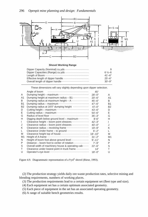
296 Open pit mine planning and design: Fundamentals
Angle of boomA Dumping height – maximumA1 Dumping height at maximum radius – B1B Dumping radius at maximum height – AB1 Dumping radius – maximumB2 Dumping radius at 16'0" dumping heightD Cutting height – maximumE Cutting radius – maximumG Radius of level floorH Digging depth below ground level – maximumI Clearance height – boom point sheavesJ Clearance radius – boom point sheavesK Clearance radius – revolving frameL Clearance Under frame – to groundM Clearance height top of houseM1 Height of A-frameN Height of boom foot above ground levelP Distance – boom foot to center of rotationS Overall width of machinery house & operating cabT Clearance under lowest point in truck frameU Operator’s eye level
45°28'–0"20'–6"45'–6"47'–6"47–0"43'–6"54'–6"35'–3"
8'-6"42'–3"40'–0"19'–9"6'–2"
18'–10"31'–2"9'–11"7'–9"
22'–6"14"
18'–0"
AA1BB1B2DEGHIJKLMM1NPSTU
E
K
D
B1
BJ
U A1A L
S
MM1
16
B2
NP
CH
Shovel Working Range
Dipper Capacity (Nominal) cu.ydsDipper Capacities (Range) cu.ydsLength of BoomEffective length of dipper handleOverall length of dipper handle
These dimensions will vary slightly depending upon dipper selection.
96 ½–641'–6"25'–6"30'–9"
Figure 4.9. Diagrammatic representation of a 9 yd3 shovel (Riese, 1993).
(2) The production strategy yields daily ore-waste production rates, selective mining andblending requirements, numbers of working places.
(3) The production requirements lead to a certain equipment set (fleet type and size).(4) Each equipment set has a certain optimum associated geometry.(5) Each piece of equipment in the set has an associated operating geometry.(6) A range of suitable bench geometries results.

Geometrical considerations 297
70
60
50
40
Hei
ght o
f Rea
ch (
ft)
30
20
10
00 10 20 30 40 50
Nominal Bucket Size (yd3)
60 70
ShovelsW
heel
Loaders
Figure 4.10. Height of reach as a function of bucket size.
Figure 4.11. Two different bench height scenarios.
(7) Consequences regarding stripping ratios, operating vs. capital costs, slope stabilityaspects, etc. are evaluated.
(8) The ‘best’ of the various alternatives is selected.In the past when rail bound equipment was being extensively used, great attention waspaid to bench geometry. Today highly mobile rubber tired/ crawler mounted equipment hasreduced the detailed evaluation requirements somewhat.
4.3 ORE ACCESS
One of the topics which is little written about in the mining literature is gaining initial physicalaccess to the orebody. How does one actually begin the process of mining? Obviously theapproach depends on the topography of the surrounding ground. To introduce the topic itwill be assumed that the ground surface is flat. The overlying vegetation has been removed

298 Open pit mine planning and design: Fundamentals
Figure 4.12. Example ore-body geometry.
Figure 4.13. Ramp access for the example orebody.
as has the soil/sand/gravel overburden. In this case it will be assumed that the orebody is700 ft in diameter, 40 ft thick, flat dipping and is exposed by removing the soil overburden.The ore is hard so that drilling and blasting is required. The bench mining situation is shownin Figure 4.12.
A vertical digging face must be established in the orebody before major production canbegin. Furthermore a ramp must be created to allow truck and loader access. A drop cutis used to create the vertical breaking face and the ramp access at the same time. Becausevertical blastholes are being fired without a vertical free face, the blast conditions are highlyconstrained. Rock movement is primarily vertically upwards with only very limited sidewaysmotion. To create satisfactory digging conditions the blastholes are normally rather closelyspaced. Here only the geometry aspects will be emphasized. To access the orebody, theramp shown in Figure 4.13 will be driven. It has an 8% grade and a width of 65 ft. Althoughnot generally the case, the walls will be assumed vertical. To reach the 40 ft desired depththe ramp in horizontal projection will be 500 ft in length. There is no general agreement onhow the drop cut should be drilled and blasted. Some companies drill the entire cut withholes of the same length. The early part of the ramp then overlies blasted rock while the finalportion is at grade. In the design shown in Figure 4.14 the drop cut has been split into threeportions. Each is blasted and loaded out before the succeeding one is shot. Rotary drilledholes 97/8
′′ in diameter are used. The minimum hole depth is 15 ft. This is maintained overthe first 90 ft of the ramp. The hole depth is then maintained at 7 ft below the desired finalcut bottom. A staggered pattern of holes is used.
The minimum width of the notch is controlled largely by the dimensions of the loadingmachine being used. In this example, it will be assumed that the loading machine is the9 yd3 capacity shovel shown diagrammatically in Figure 4.9.

Geometrical considerations 299
Figure 4.14. Blast design for the ramp excavation.
In the generally tight confines of the drop cut the following shovel dimensions:K , the clearance radius of the revolving frame,J , the clearance radius of the boom point sheaves,G, the maximum digging radius of the level floor, andE, the maximum cutting radius
are of importance. As can be seen from Figure 4.9, these are:
K = 19′9′′
J = 40′0′′
G = 35′3′′
E = 54′6′′
The minimum width of the drop cut is given by
Minimum width = K + J
In this case it is
Minimum width = 19′9′′ + 40′0′′ = 59′9′′
This is such that both the front and rear portions of the machine can clear the banks on thetwo sides as it revolves in the digging and dumping modes.
The maximum digging radius of the level floor is used to indicate the maximum dropcut width for the shovel working along one cutting path. The maximum value is that whichthe shovel dipper (bucket) can be moved horizontally outward, thereby accomplishing floorcleanup.
The maximum width of the cut at floor level would be
Maximum cut width (floor) = 2 × 35′3′′ = 70′6′′
The maximum width of the cut at crest level would be
Maximum cut width (crest) = 2 × 54′6′′ = 109′
In practice the cutting width for the shovel moving along one path is relatively tightlyconstrained by the shovel dimensions. In this case:
Minimum cut width (crest) ∼= 60 ft
Maximum cut width (floor) ∼= 71 ft
Maximum cut width (crest) = 109 ft

300 Open pit mine planning and design: Fundamentals
For typical cut slope angles of 60 to 80◦, the maximum cut width (floor) is the controllingdimension. When the cutting path is down the center of the cut and the shovel is digging toboth sides the maximum floor and minimum crest radii would be
Maximum floor radius = 35′3′′
Minimum crest radius = 40′0′′
In any case, for laying out the blasting round and evaluating minimum pit bottom dimensionsone wants to exceed the minimum working space requirements.
Figures 4.15A through 4.15D show the minimum floor bottom geometry when the shovelmoves along the two cutting paths. The loading would first be from one bank. The shovelwould then move over and load from the other. This would be considered very tight operatingconditions and would be used to create a final cut at the pit bottom.
The usual drop cut is shown in Figures 4.16A through 4.16C where the shovel movesalong the cut centerline and can dig to both sides. It will be noted that the shovel must swingthrough large angles in order to reach the truck.
In both cases the working bench geometry at this stage is characterized by crampedoperating conditions.
Two locations for the drop cut/ramp will be considered. The first (case A) is entirely inthe waste surrounding the pit. It is desired to have the floor of the ramp at the bottom of orejust as it reaches the ore-waste contact. This is shown diagrammatically in Figure 4.17. Thevolume of waste rock mined in excavating the ramp is
Ramp volume = 1
2H
100H
gRW
where RW is the average ramp width, H is the bench height, and g is the road grade (%).In this case it becomes
Ramp volume = 1
2
(40)2 × 100 × 65
8= 650, 000 ft3
This waste must be excavated and paid for before any ore can be removed. However inthis arrangement all of the ore can be removed. If it is assumed that the orebody can beextracted with vertical walls, then the ore volume extracted is
Ore volume = πD2H
4= π
4(700)2 × 40 = 15, 400, 000 ft3
Upon entering the orebody mining proceeds on an ever expanding front (Fig. 4.18).As the front expands the number of loading machines which can effectively operate at
the same time increases. Hence the production capacity for the level varies with time.In summary for this ramp placement (case A):
Waste removed (road) = 650,000 ft3
Ore extracted = 15,400,000 ft3
% ore extracted = 100%
Another possibility (case B) as is shown in Figure 4.19 is to place the ramp in ore ratherthan to place the ramp in waste rock. This would be driven as a drop cut in the same wayas discussed earlier. The volume excavated is obviously the same as before but now it isore. Since the material is ore it can be processed and thereby profits are realized earlier.
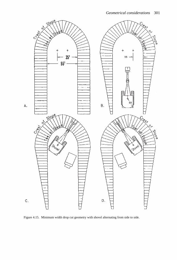
Geometrical considerations 301
Figure 4.15. Minimum width drop cut geometry with shovel alternating from side to side.

Open pit mine planning and design: Fundamentals
Figure 4.16. Minimum width drop cut geometry with shovel moving along centerline.
From the ramp bottom, the extraction front is gradually increased in length (Fig. 4.20).Obviously the disadvantage is that when mining is completed a quantity of ore remainslocked up in the ramp. This quantity is equal to the amount of waste extracted in case A.
Thus the two important points to be made are:– If the haul road is added external to the planned pit boundaries, then an additional
quantity of material equal to the volume of the road must be extracted.
302

Geometrical considerations
Figure 4.17. Isometric view of the rampin waste approaching the orebody.
Figure 4.18. Diagrammatic representa-tion of the expanding mining front.
Figure 4.19. Dropcut/ramp placement in ore. Figure 4.20. Expansion of the mining front.
– If the haul road is added internal to the original planned boundaries, then a quantity ofmaterial equal to the road volume must be left in place.
Rather than a straight road such as shown in case A, one might have considered a curvedroad such as shown in plan in Figure 4.21. With the exception of the final portion, the roadis entirely driven in waste. The road could be placed so that the ‘ore’ left is in the poorestgrade.
Assume that the pit is not 1 bench high but instead consists of 2 benches such as is shownin Figure 4.22. The idea is obviously to drive the ramp down to the ore level and establish
303

Open pit mine planning and design: Fundamentals
Figure 4.21. Ramp starting in waste andending in ore. Figure 4.22. Section through a two bench mine.
Figure 4.23. Two ramp sections withpit expansion.
the desired production rate. Then while mining is underway on level 1, the ramp would beextended in ore to the lower level as shown in Figure 4.23 through the use of a drop cut.All of the ore lying below the ramp is obviously sterilized. For a multi-bench operation, theprocedure continues as shown in Figure 4.24. Note that a flat section having a length of 200 fthas been left in this example between the decline segments. The ramp has a corkscrew shapeand the coils get tighter and tighter as the pit is deepened. Rather soon in this example, thepit would reach a final depth simply because the ramp absorbed all of the available workingspace.
A vertical section taken through the final pit with the orebody superimposed is shown inFigure 4.25. For this particular design where only the initial segment of the ramp is in waste,a large portion of the orebody is sterilized. The amount of waste removed is minimized,however.
An alternative design is one where the ramp is underlain by waste and all of the ore isremoved. To make this construction one starts the road design at the lowest bench and worksback out. This exercise is left to the reader.
The actual design will generally be somewhere in between these two alternatives with theupper part of the ramp underlain by waste and the lower part by ‘ore’.
304

Geometrical considerations
Figure 4.24. Plan view showing ramp locations fora five bench mine.
Figure 4.25. Section view showing the sterilization of reserves by ramp.
The excavation may start with attacking the ore first so that the cash flow is improved.Later during the mine life, the waste will be stripped as the main access is gradually movedoutward.
In summary:– there can be considerable volumes associated with the main ramp system;– the location of the ramp changes with time;– in the upper levels of the pit, the ramp is underlain by waste; in the lower ranges it is
underlain by mineral;– cash flow considerations are significantly affected by ramp timing;– the stripping ratio, the percent extraction and the overall extraction are strongly affected
simply by the haul road geometry (road width and road grade).Drop cuts are used on every level to create a new bench. Figures 4.26A through 4.26D
show the steps going from the current pit bottom through the mining out of the level. Oftenthe ramp is extended directly off of the current ramp and close to the existing pit wall. This isshown in Figure 4.27. A two level loading operation is shown isometrically in Figure 4.28.The ramp access to both levels in this relatively simple example is easily seen.
305

Open pit mine planning and design: Fundamentals
5575
5575
5600
5575A.
100 100 2000
SCALE IN FEET
100 100 2000
SCALE IN FEET
5575
5550
5575
Ramp
Ramp
5575
5575
5600B.
5550
5550
5600Ramp
5575
5550
5600
5550
5550
5575
5575
5600
Ramp
C. D.
Ramp
5550
5575
5575
5575
Ramp
5600
5600
Figure 4.26. Plan view of an actual pit bottom showing drop cut and mining expansion (McWilliams, 1959).
There are many examples where the orebody lies in very rugged terrain. Figure 4.29 showsdiagrammatically one possible case. Here the entry to the orebody is made by pushing backthe hillside. Bench elevations are first established as shown on the figure. In this case thebench height is 50 ft. Initial benches are established by making pioneering cuts along thesurface at convenient bench elevations.
306

Geometrical considerations
LEGEND
CrestToe
Bench limitHoulage road
55005433
5400
RA
MP
RA
MP
5433
5400
5433
5500
54005467
RAMP
300 5500 RAMP
5433
5525 RAMP
5L
5450 55
00
5367
RA
MP
Figure 4.27. Extension of the current ramp close to the pit wall (McWilliams, 1959).
If the slope is composed of softer material, then a dozer can notch it without further assis-tance (Fig. 4.30). For harder rock types, ripping prior to dozing may be enough. Howeverif the rock is hard or the slope is steep, drilling and blasting will probably be necessary forthe pioneer cut. Generally air track types of drills are used. They can reach and drill in verydifficult places and can tow their own air compressors/generators.
As shown in Figure 4.31 a shovel can be used instead of a dozer for notching a slope. Thenotch is enlarged by taking successive cuts until the full bench height is achieved.
Once these initial benches are established, mining of the full faces with vertical blastholes proceeds. Obviously the upper benches have to be advanced before the lowerones.
The final pit outline for this section is shown in Figure 4.33. The reader is encouraged toconsider the pit development sequence and the point where drop cuts would be used.
307

Open pit mine planning and design: Fundamentals
Figure 4.28. Isometric view of simultaneous mining on several levels (Tamrock, 1978).
Figure 4.29. Deposit located in mountainous terrain.
308

Geometrical considerations
Figure 4.30. Creating initial access/benches (Nichols,1956).
Figure 4.31. Sidehill cut with a shovel (Nichols, 1956).
Cut #2
Cut #6
Cut #5
Cut #4
Cut #3
Cut #2Cut #1
Cut #1 Cut #4
Cut #3Road #1
Road #2
Road #1
Road #2
#2#1
#5#4
#3
#6
#6#5
#9#8 #7
#3#2
#10
Figure 4.32. Shovel cut sequence when initiating benching in a hilly terrain (Nichols, 1956).
309
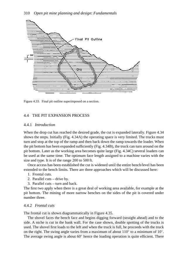
Open pit mine planning and design: Fundamentals
Figure 4.33. Final pit outline superimposed on a section.
4.4 THE PIT EXPANSION PROCESS
4.4.1 Introduction
When the drop cut has reached the desired grade, the cut is expanded laterally. Figure 4.34shows the steps. Initially (Fig. 4.34A) the operating space is very limited. The trucks mustturn and stop at the top of the ramp and then back down the ramp towards the loader. Whenthe pit bottom has been expanded sufficiently (Fig. 4.34B), the truck can turn around on thepit bottom. Later as the working area becomes quite large (Fig. 4.34C) several loaders canbe used at the same time. The optimum face length assigned to a machine varies with thesize and type. It is of the range 200 to 500 ft.
Once access has been established the cut is widened until the entire bench/level has beenextended to the bench limits. There are three approaches which will be discussed here:
1. Frontal cuts.2. Parallel cuts – drive by.3. Parallel cuts – turn and back.
The first two apply when there is a great deal of working area available, for example at thepit bottom. The mining of more narrow benches on the sides of the pit is covered undernumber three.
4.4.2 Frontal cuts
The frontal cut is shown diagrammatically in Figure 4.35.The shovel faces the bench face and begins digging forward (straight ahead) and to the
side. A niche is cut in the bank wall. For the case shown, double spotting of the trucks isused. The shovel first loads to the left and when the truck is full, he proceeds with the truckon the right. The swing angle varies from a maximum of about 110◦ to a minimum of 10◦.The average swing angle is about 60◦ hence the loading operation is quite efficient. There
310

Geometrical considerations
Figure 4.34. Detailed steps in the develop-ment of a new production level (Carson, 1961).
Cre
stof
Slope
Toe
ofSlop
e
Shovel
Figure 4.35. Diagrammatic representation of a frontal cutting operation.
must be room for the trucks to position themselves around the shovel. The shovel penetratesto the point that the center of swing is in line with the face. It then moves parallel to itselfand takes another frontal cut (Fig. 4.36).
With a long face and sufficient bench width, more than one shovel can work the sameface (Fig. 4.37). A fill-in cut is taken between the individual face positions (Fig. 4.38). Fromthe shovels view point this is a highly efficient loading operation. The trucks must howeverstop and back into position.
311

Open pit mine planning and design: Fundamentals
Cre
stof
Slope
Toe
ofSlop
e
Shovel
Figure 4.36. Shovel move to adjacent cutting position.
Cre
stof
Slope
Toe
ofSlop
e
Shovel35.3'
Cre
stof
SlopeTo
eof
Slope
Shovel35.3'
Figure 4.37. Two shovels working the same face.
Cre
stof
Slope
Cre
stof
Slope
Toe
ofSlop
e
Toe
ofSlop
e
Shovel Shovel35.3' 35.3'
Figure 4.38. Fill-in cutting to complete the face.
312

Geometrical considerations
Figure 4.39. Parallel cut with drive-by.
4.4.3 Drive-by cuts
Another possibility when the mine geometry allows is the parallel cut with drive-by. This isshown diagrammatically in Figure 4.39. The shovel moves across and parallel to the diggingface. For this case, bench access for the haul units must be available from both directions.It is highly efficient for both the trucks and the loader. Although the average swing angle isgreater than for the frontal cut, the trucks do not have to back up to the shovel and spottingis simplified.
4.4.4 Parallel cuts
The expansion of the pit at the upper levels is generally accomplished using parallel cuts.Due to space limitations there is only access to the ramp from one side of the shovel. Thismeans that the trucks approach the shovel from the rear. They then stop, turn and back intoload position. Sometimes there is room for the double spotting of trucks (Fig. 4.40) andsometimes for only single spotting (Fig. 4.41).
Pit geometry is made up of a series of trade-offs. Steeper slopes result in a savings ofstripping costs. On the other hand they can, by reducing operating space, produce an increasein operating costs.
Figure 4.42 shows the single spotting sequence. Truck 2 (Fig. 4.42B) waits while theshovel completes the loading of truck 1. After truck 1 has departed (Fig. 4.42C), truck 2turns and stops (Fig. 4.42D) and backs into position (Fig. 4.42E). While truck 2 is being
313

Open pit mine planning and design: Fundamentals
Figure 4.40. Parallel cut with the double spotting of trucks.
Figure 4.41. Parallel cut with the single spotting of trucks.
314

Geometrical considerations
Figure 4.42. Time sequence showing shovel loading with single spotting.
315

Open pit mine planning and design: Fundamentals
Figure 4.42. (Continued).
loaded truck 3 arrives (Fig. 4.42F). The process then repeats. In this situation both the trucksand the shovel must wait causing a reduction in the overall productivity.
The double spotting situation is shown in Figure 4.43. Truck 1 is first to be loaded(Fig. 4.43A).
Truck 2 arrives (Fig. 4.43B) and backs into position (Fig. 4.43C). When it is just inposition the shovel has completed the loading of truck 1. As truck 1 departs (Fig. 4.43D)the shovel begins the loading of truck 2. As truck 2 is being loaded truck 3 arrives. It turns(Fig. 4.43E) and backs into position (Fig. 4.43F).As truck 2 leaves the shovel begins loadingtruck 3 (Fig. 4.43G). With this type of arrangement there is no waiting by the shovel andless waiting by the trucks. Thus the overall productivity of this system is higher than that forsingle spotting. The sequencing is unfortunately quite often not as the theory would suggest.Figures 4.43H and 4.43I show two rather typical situations. Both of these can be minimizedthrough the use of an effective communications/dispatching system.
4.4.5 Minimum required operating room for parallel cuts
In the previous section the physical process by which a pit is expanded using parallel cutswas described. In this section, the focus will be on determining the amount of operat-ing room required to accommodate the large trucks and shovels involved in the loadingoperation.
The dimension being sought is the width of the working bench. The working bench isthat bench in the process of being mined. This width (which is synonymous with the term‘operating room’) is defined as the distance from the crest of the bench providing the floor
316

Geometrical considerations
Figure 4.43. Time sequence showing shovel loading with double spotting.
for the loading operations to the bench toe being created as the parallel cut is being advanced.The minimum amount of operating room varies depending upon whether single or doublespotting of trucks is used, with the latter obviously requiring somewhat more. The minimumwidth (WB) is equal to the width of the minimum required safety bench (SB) plus the widthof the cut (WC) being taken. This is expressed as
WB = SB + WC
317

Open pit mine planning and design: Fundamentals
Figure 4.43. (Continued).
The easiest way of demonstrating the principles involved is by way of example. For this,the following assumptions will be made:
– Bench height = 40 ft.– A safety berm is required.– The minimum clearance between the outer truck tire and the safety berm = 5 ft.– Single spotting is used.– Bench face angle = 70◦.– Loading is done with a 9 yd3 BE 155 shovel (specifications given in Fig. 4.9).– Haulage is by 85 ton capacity trucks.
318

Geometrical considerations
Figure 4.43. (Continued).
– Truck width = 16 ft.– Tire rolling radius = 4 ft.
The general arrangement in plan and section is shown in Figure 4.44. The design showsthat:
Working bench width = 102 ft
Cut width = 60 ft
Safety bench width = 42 ft
The basic calculations ( justification) behind these numbers will now be presented.
Step 1. A safety berm is required along the edge of this bench. As will be discussed inSubsection 4.9.5, the height of the berm should be of the order of the tire rolling radius.For this truck, the berm height would be about 4 ft. Assuming that the material has an angleof repose of 45◦, the width of the safety berm is 8 ft (see Fig. 4.45). It is assumed that thisberm is located with the outer edge at the crest.
Step 2. The distance from the crest to the truck centerline is determined assuming parallelalignment. A 5′ clearance distance between the safety berm and the wheels has been used.Since the truck is 16 ft wide, the centerline to crest distance (TC) is 21 ft.
Step 3. The appropriate shovel dimensions are read from the specification sheet (Fig. 4.9):
(a) Shovel centerline to truck centerline. This is assumed to be the dumping radius (B) atmaximum height,
B = 45′6′′ = 45.5 ft
319

320 Open pit mine planning and design: Fundamentals
Figure 4.44. Section and plan views through a working bench.
Figure 4.45. Simplified representation of a safety berm.
(b) The maximum dumping height (A) is more than sufficient to clear the truck,
A = 28 ft
(c) The level floor radius dimension (G) is the maximum distance from the shovelcenterline which the floor can be cleaned. In this case
G = 35′3′′ = 35.25 ft
This will be used as the maximum shovel centerline to toe distance.

Geometrical considerations 321
Step 4. The desired working bench dimension becomes
WB = TC + B + G = 21 + 45.5 + 35.25 ∼= 102 ft
Step 5. The corresponding width of cut is now calculated. In this case it has been assumedthat the shovel moves along a single path parallel to the crest. Information from the shovelmanufacturer suggests that the maximum cutting width (WC) may be estimated by
WC = 0.90 × 2 × G = 0.90 × 2 × 35.25 ∼= 63.5 ft
This applies to the width of the pile of broken material. Therefore, to allow for swell andthrow of the material during blasting, the design cut width should be less than this value.Here a value of 60 ft has been assumed.
Step 6. Knowing the width of the working bench and the cut width, the resulting safetybench has a width
SB = 102 − 60 = 42 ft
This is of the order of the bench height (40 ft) which is a rule of thumb sometimes employed.
Step 7. Some check calculations are made with regard to other dimensions.
a) The maximum cutting height of the shovel
D = 43′6′′ = 43.5 ft
is greater than the 40′ bench height. Thus the shovel can reach to the top of the bench facefor scaling.
b) The maximum shovel cutting radius (E) is
E = 54′6′′ = 54.5 ft
Since the maximum radius of the level floor (G) is
G = 35′3′′ = 35.25 ft
the flattest bench face angle which could be scaled (Fig. 4.46) is
Slope = tan−1 40
54.50 − 35.25= 64.3◦
Thus the shovel can easily scale the 70◦ bench face.
Step 8. The cut dimension should be compared to the drilling and blasting pattern being used.In this particular case the holes are 121/4 ins. in diameter (De) and ANFO is the explosive.Using a common rule of thumb, the burden (B) is given by
B = 25De
12∼= 25 ft
The hole spacing (S) is equal to the burden
S = 25 ft
Thus two rows of holes are appropriate for this cut width.

322 Open pit mine planning and design: Fundamentals
Figure 4.46. The bench/bench face geometry for the example.
A somewhat simplified approach has been applied to the matter of determining workingbench width. The complications arise when one examines the best width from an overalleconomic viewpoint.
As will be discussed in Section 4.5, the working bench is generally one of a set of 3 to 5benches being mined as a group. The others in the set each have a width equal to that of asafety bench. As the cut is extracted, the remaining portion of the working bench is reducedto a safety bench width. Since the width of the working bench is approximately equal to thecombined widths of the others in the set, it has a major impact on the overall slope angle.A wider working bench means that the slope angle is flatter with the extra costs related toearlier/more stripping, but the equipment operating efficiency is higher (with lower relatedcosts). On the other hand a more narrow working bench would provide a steeper overallslope at the cost of operating efficiency. Thus, there are other factors, beside those relatedto equipment geometries, which must be considered.
4.4.6 Cut sequencing
In the previous section the terms ‘working bench,’ ‘cut’ and ‘safety bench’ were introduced.These will now be applied to a simple example in which a 90 ft wide cut 1000 ft long willbe taken from the right hand wall of the pit shown in Figure 4.47. As can be seen the wallconsists of 4 benches. The entire bench 1 (B1) is exposed at the surface. Benches B2, B3and B4 are safety benches, 35 ft wide. The process begins with the drill working off theupper surface of B1. The holes forming the cut to be taken from B1 are drilled and blasted(Fig. 4.48). The shovel then moves along the floor of bench B1 (upper surface of B2) andloads the trucks which also travel on this surface. The working bench has a width of 125 ft.When the cut is completed the geometry is as shown in Figure 4.49. The cut to be takenfrom bench 2 is now drilled and blasted. The shovel moves along the top of bench 3 takinga cut width (WC). A portion of bench 2 remains as a safety bench. The process is repeateduntil the bottom of the pit is reached. The shovel then moves back up to bench 1 and theprocess is repeated. If it is assumed that the shovel can produce 10,000 tons/day, then theoverall production from these 4 benches is 10,000 tons/day. The four benches associatedwith this shovel are referred to as a mine production unit.

Geometrical considerations 323
Pit surface
Bench 1
Bench 2
Bench 3
Bench 4 Figure 4.47. Initial geometry for the push backexample.
Bench 1
Bench 2
Bench 3
Bench 4
Upper surface
Lower surface (floor)
DB
Cut 1
WB
BθAB Figure 4.48. Cut mining
from bench 1.
Bench 1
Bench 2
Bench 3
Bench 4
Cut 2
θA�B
WB
DB
A�
B Figure 4.49. Cut mining from bench 2.
4.5 PIT SLOPE GEOMETRY
There are a number of ‘slopes’ which enter into pit design. Care is needed so that there isno confusion as to how they are calculated and what they mean. One slope has already beenintroduced. That is the bench face angle (Fig. 4.50). It is defined as the angle made with thehorizontal of the line connecting the toe to the crest. This definition of the slope going fromthe toe to the crest will be maintained throughout this book.
Now consider the slope consisting of 5 such benches (Fig. 4.51). The angle made withthe horizontal of the line connecting the lowest most toe to the upper most crest is definedas the overall pit slope,
�(overall) = tan−1 5 × 50
4 × 35 + 5×50tan 75◦
= 50.4◦

324 Open pit mine planning and design: Fundamentals
35'Crest
50'
75˚ toe
13.4'Figure 4.50. Safety bench geometry showingbench face angle.
upper most crest
35'
35'
75° 35'
50'
35'
lowest most toe
overallslopeangle
θ
13.4'
250'
Figure 4.51. Overall slope angle.
If as is shown in Figure 4.52 an access ramp with a width of 100 ft is located half way upbench 3, the overall pit slope becomes
�(overall) = tan−1 5 × 50
4 × 35 + 5×50tan 75◦ + 100
= 39.2◦
As can be seen, the presence of the ramp on a given section has an enormous impact on theoverall slope angle.
The ramp breaks the overall slope into two portions (Fig. 4.53) which can each bedescribed by slope angles. These angles are called interramp angles (between-the-rampangles). In this case
IR1 = IR2 = tan−1 125
2 × 35 + 2×50tan 75◦ + 25
tan 75◦= 50.4◦

Geometrical considerations 325
35'
35'
35'
35'
Ramp100'
75°
50°
overallslopeangle
13.4'
250'
Figure 4.52. Overall slope angle with ramp included.
Crest
35'
35'
Ramp100'25' θIR1
θIR2
25'35'
35'
Toe
50'
75°
Ramp Crest
13.4'
250'
Ramp Toe
Figure 4.53. Interramp slope angles for Figure 4.52.

326 Open pit mine planning and design: Fundamentals
250'
125'
35'
35'
50'
35'
75°
overallslopeangle
13.4'
θ
Figure 4.54. Overall slope angle with working bench included.
The interramp wall height is 125 ft for each segment. Generally the interramp wall heightsand angles for the different slope segments would not be the same. From a slope stabilityviewpoint each interramp segment would be examined separately.
While active mining is underway, some working benches would be included in the overallslope. Figure 4.54 shows a working bench 125 ft in width included as bench 2. The overallslope angle is now
� = tan−1 5 × 50
125 + 4 × 35 + 5×50tan 75◦
= 37.0◦
The working bench is treated in the same way as a ramp in terms of interrupting the slope.The two interramp angles are shown in Figure 4.55. In this case
�IR1 = 75◦
�IR2 = tan−1 200
3 × 35 + 4×50tan 75◦
= 51.6◦
The interramp wall heights are
H1 = 50′
H2 = 200′
For this section, it is possible that the ramp cuts bench 3 as before. This situation is shownin Figure 4.56.
The overall slope angle has now decreased to
� = tan−1 250
125 + 3 × 35 + 100 + 5×50tan 75◦
= 32.2◦

Geometrical considerations 327
θIR1
θIR2
125'
35'
75° 35'
50'
35'
13.4'
250'
Figure 4.55. Interramp angles associated with the working bench.
Working Bench
125'
35'
35'
50'
35'
Ramp100'
75°250'
overallslopeangle
θ
13.4'
Figure 4.56. Overall slope angle with one working bench and a ramp section.
As shown in Figure 4.57, there are now three interramp portions of the slope. The interrampwall heights and angles are:
Segment 1:
�IR1 = 75◦
H = 50′

328 Open pit mine planning and design: Fundamentals
250'
θIR1
θIR2
θIR3
125'
35'
75° 35'
50'
35'
13.4'
Working Bench
Ramp100'
Figure 4.57. Interramp slope angles for a slope containing a working bench and a ramp.
Segment 2:
�IR2 = tan−1 75
35 + 75tan 75◦
= 35.7◦
H = 75′
Segment 3:
�IR3 = tan−1 125
2 × 35 + 125tan 75◦
= 50.4◦
H = 125′
In Figure 4.57, the overall slope is shown to contain one working bench. Under somecircumstances there may be several working benches involved in the mining of the slope.Figure 4.58 shows the case of a slope with 6 benches of which two are working benches125 ft in width.
The overall (working slope) is given by
� = tan−1 300
3 × 35 + 2 × 125 + 300tan 75◦
= 34.6◦
The slope associated with each shovel working group is shown in Figure 4.59. In this caseit is
� = tan−1 150
125 + 35 + 150tan 75◦
= 36.8◦
If the number of working benches is increased to 3 for the slope containing 6 benches, theoverall slope would be further reduced. Thus to maintain reasonable slope angles, mostmines have one working bench for a group of 4 to 5 benches.

Geom
etrical considerations 329
ShovelGroup
#1
300'
150'
35'
125'
35'
Working Bench #275°
Working Bench #1
125'
50'
35'
overallslopeangle θ
13.4'
150'ShovelGroup
#2
Figure 4.58. Overall slope angle for a slope containing two working benches.

330 O
pen pit mine planning and design: F
undamentals
ShovelGroup
#1150'
35'
Working Bench #1125'
θWG
θWG
35'
Working Bench #2
300'
ShovelGroup
#2150'
75° 125'
50'
35'
13.4'
Figure 4.59. Slopes for each working group.

Geometrical considerations
250' 50'
75°
17'
final(overall)
angleθ
Figure 4.60. Final overall pit slope.
At the end of mining it is desired to leave the final slope as steep as possible. Some ofthe safety benches will be reduced in width while others may be eliminated entirely. Forfinal walls, a bench width of approximately 1/3 of the bench height is commonly used. Forthis example with a bench height of 50 ft, the bench width becomes 17 ft. The final pit slopeangle, assuming no ramp is needed on this wall (Fig. 4.60), becomes
�(final) = tan−1 250
4 × 17 + 250tan 75◦
= 61.6◦
If the final bench faces could have been cut at 90◦ instead of 75◦, then the final overallpit slope angle would be
�(final) = tan−1 250
4 × 17= 74.8◦
It is much more likely that the final face angles are 60◦ and the safety benches 20 ft wide.This gives
�(final) = tan−1 250
4 × 20 + 250tan 60◦
= 48◦
Although much regarding final slope angles has to do with rock structure, care in blastingcan make a major impact.
331

3 Open pit mine planning and design: Fundamentals
Table 4.2. Classification of open pit slope problems (Hoek, 1970b).
Category Conditions Method of solution
A. Unimportant Mining a shallow high grade orebody in favorable No consideration ofslopes geological and climatic conditions. Slope angles slope stability
unimportant economically and flat slopes can be used. required.B. Average Mining a variable grade orebody in reasonable geological Approximate
slopes and climatic conditions. Slope angles important but not analysis of slopecritical in determining economics of mining. stability normally
adequate.C. Critical Mining a low grade orebody in unfavorable geological and Detailed geological
slopes climatic conditions. Slope angles critical in terms of both and groundwatereconomics of mining and safety of operation. studies followed by
comprehensivestability analysisusually required.
4.6 FINAL PIT SLOPE ANGLES
4.6.1 Introduction
During the early feasibility studies for a proposed open pit mine, an estimate of the safeslope angles is required for the calculation of ore to waste ratios and for the preliminary pitlayout. At this stage generally the only structural information available upon which to basesuch an estimate is that obtained from diamond drill cores collected for mineral evaluationpurposes. Sometimes data from surface outcrops are also available. How well these finalslope angles must be known and the techniques used to estimate them depends upon theconditions (Table 4.2) applicable. During the evaluation stage for categories B and C, thebest engineering estimate of the steepest safe slope at the pit limits in each pit segment isused. Since the information is so limited, they are hedged with a contingency factor. If theproperty is large and has a reasonably long lifetime, initially the exact slope angles are ofrelatively minor importance. The effect of steeper slopes at the pit limits is to increase theamount of ore that can be mined and therefore increase the life of the mine. The effect ofprofits far in the future has practically no impact on the net present value of the property.
During the pre-production period and the first few years of production, the operating slopesshould however be as steep as possible while still providing ample bench room for optimumoperating efficiency. The minimization of stripping at this stage has a significant effect onthe overall economics of the operation. The working slopes can then be flattened until theyreach the outer surface intercepts. Steepening operations then commence to achieve thefinal pit slopes (Halls, 1970). Cases do occur where the viability of an orebody is highlydependent on the safe slope angle that can be maintained. Special measures, including thecollection of drillhole data simply for making slope determinations are then taken.
There are a number of excellent references which deal in great detail with the design ofpit slopes. In particular Rock Slope Engineering by Hoek & Bray (1977), and the series ofpublications developed within the Pit Slope Manual series produced by CANMET shouldbe mentioned. This brief section focusses on a few of the underlying concepts, and presentssome curves extracted largely from the work of Hoek (1970a, 1970b) which may be usedfor making very preliminary estimates.
32

Geometrical considerations 333
Figure 4.61. Horizontal stress redistribution due to the creation of a pit.
4.6.2 Geomechanical background
Figure 4.61 shows diagrammatically the horizontal flow of stress through a particular verticalsection both with and without the presence of the final pit. With the excavation of the pit,the pre-existing horizontal stresses are forced to flow beneath the pit bottom (and aroundthe pit ends).
The vertical stresses are also reduced through the removal of the rock overlying the finalslopes. This means that the rock lying between the pit outline and these flow lines is largelydistressed. As a result of stress removal, cracks/joints can open with a subsequent reductionin the cohesive and friction forces restraining the rock in place. Furthermore, ground watercan more easily flow through these zones, reducing the effective normal force on potentialfailure planes. As the pit is deepened, the extent of this destressed zone increases, andthe consequences of a failure becomes more severe. The chances of encountering adversestructures (faults, dykes, weakness zones, etc.) within these zones increase as well. Finally,with increasing pit depth, the relative sizes of the individual structural blocks making up theslopes become small compared to the overall volume involved. Thus the failure mechanismmay change from one of structural control to one controlled by the characteristics of agranular mass. Figure 4.62 shows the four major types of failure which occur in an open
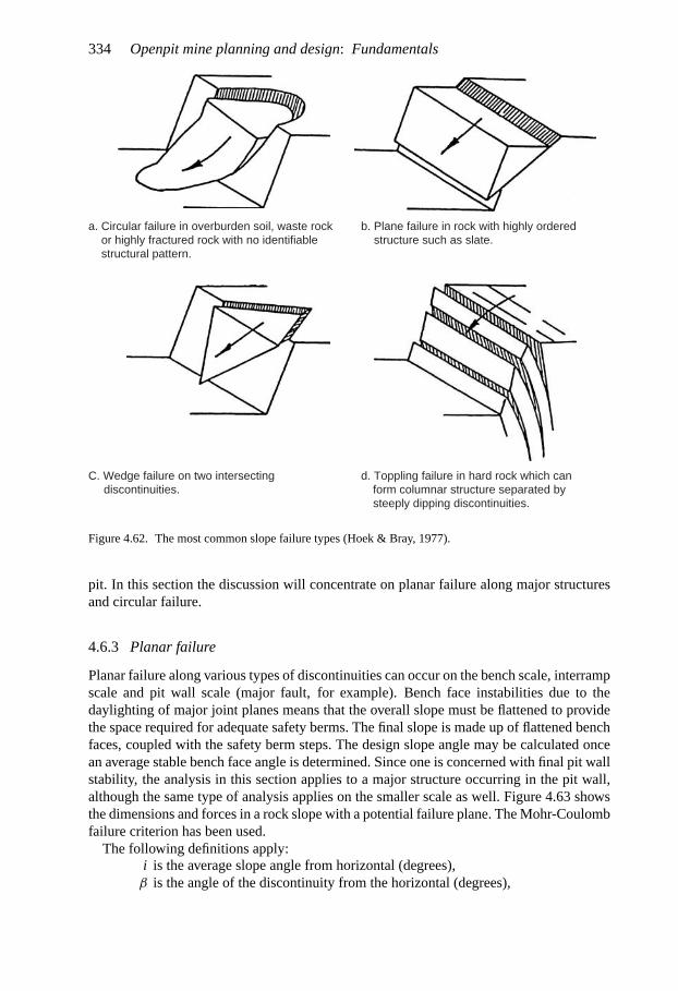
334 Open pit mine planning and design: Fundamentals
a. Circular failure in overburden soil, waste rock or highly fractured rock with no identifiable structural pattern.
b. Plane failure in rock with highly ordered structure such as slate.
C. Wedge failure on two intersecting discontinuities.
d. Toppling failure in hard rock which can form columnar structure separated by steeply dipping discontinuities.
Figure 4.62. The most common slope failure types (Hoek & Bray, 1977).
pit. In this section the discussion will concentrate on planar failure along major structuresand circular failure.
4.6.3 Planar failure
Planar failure along various types of discontinuities can occur on the bench scale, interrampscale and pit wall scale (major fault, for example). Bench face instabilities due to thedaylighting of major joint planes means that the overall slope must be flattened to providethe space required for adequate safety berms. The final slope is made up of flattened benchfaces, coupled with the safety berm steps. The design slope angle may be calculated oncean average stable bench face angle is determined. Since one is concerned with final pit wallstability, the analysis in this section applies to a major structure occurring in the pit wall,although the same type of analysis applies on the smaller scale as well. Figure 4.63 showsthe dimensions and forces in a rock slope with a potential failure plane. The Mohr-Coulombfailure criterion has been used.
The following definitions apply:i is the average slope angle from horizontal (degrees),β is the angle of the discontinuity from the horizontal (degrees),

Geometrical considerations 335
Figure 4.63. Dimensions and forces in a rock slope with a potential failure plane (Hoek, 1970a).
W is the block weight,R is the resisting force,c is the cohesion,φ is the friction angle,
W cos β is the normal force,W sin β is the driving force,
A is the area of the failure plane.
The factor of safety (F) is defined by
F = Total force available to resist sliding
Force tending to induce sliding(4.1)
For the case shown in Figure 4.63 (drained slope) Equation (4.1) becomes
F = cA + W cos β tan φ
W sin β(4.2)
If there is water present, then the factor of safety is expressed as
F = cA + (W cos β − U) tan φa
W sin β + V(4.3)
where U is the uplift force along the base of the block due to water pressure, and V is thehorizontal force along the face of the block due to water in the tension crack, φa is the frictionangle (as affected by the water). Typical values for the cohesive strength and friction anglesof soils and rock are given in Tables 4.3 and 4.4. As the height H of the slope increasesthe relative contribution of the cohesion to the total resistance decreases. For very highslopes, the stable slope angle approaches the friction angle φ. Hoek (1970a) has presentedthe relationship between slope height and slope angle functions for plane failure in a drainedslope given in Figure 4.64.
Assume for example that the average planned slope angle i is 70◦, the orientation of thepotential failure plane β is 50◦ and the friction angle φ is 30◦. Thus
X = 2√
(i − β)(β − φ) = 2√
20 × 20 = 40◦
From Figure 4.64 the slope height function Y is read as
Y = 14

336 Open pit mine planning and design: Fundamentals
Table 4.3. Cohesive strengths for ‘intact’ soil and rock (Robertson, 1971).
Material description c (lb/ft2) c (kg/m2)
Very soft soil 35 170Soft soil 70 340Firm soil 180 880Stiff soil 450 2200Very stiff soil 1600 7800Very soft rock 3500 17,000Soft rock 11,500 56,000Hard rock 35,000 170,000Very hard rock 115,000 560,000Very very hard rock 230,000 1,000,000
Table 4.4. Friction angles (degrees) for typical rock materials (Hoek, 1970a).
Rock Intact rock φ Joint φ Residual φ
Andesite 45 31–35 28–30Basalt 48–50 47Chalk 35–41Diorite 53–55Granite 50–64 31–33Graywacke 45–50Limestone 30–60 33–37Monzonite 48–65 28–32Porphyry 40 30–34Quartzite 64 44 26–34Sandstone 45–50 27–38 25–34Schist 26–70Shale 45–64 37 27–32Siltstone 50 43Slate 45–60 24–34
Other materials Approximate φ
Clay gouge (remoulded) 10–20Calcitic shear zone material 20–27Shale fault material 14–22Hard rock breccia 22–30Compacted hard rock aggregate 40Hard rock fill 38
Knowing that
c = 1600 lb/ft2
γ = 160 lb/ft3
the limiting (F = 1) slope height H with such a structure passing through the toe is foundusing
Y = 14 = γH
c= 160
1600H

Geometrical considerations 337
Figure 4.64. Relationship between slope height and slope angle functions for plane failure in a drainedslope (Hoek, 1970a).
Thus
H = 140 ft
If the planned pit depth is 500 ft, one could determine the limiting (F = 1) pit slope angle.The slope height function is
Y = γH
c= 160 × 500
1600= 50
From Figure 4.64 one finds that
X = 17.5
Solving for i yields
i = 57.7◦
The general family of curves corresponding to various safety factors is given inFigure 4.65.

338 Open pit mine planning and design: Fundamentals
Figure 4.65. Slope design chart for plane failure including various safety factors (Hoek, 1970a).
The question naturally arises as to what an appropriate safety factor might be? Thisdepends on the confidence one has in the ‘goodness’ of the input data and also on thefunction of the structure. Jennings & Black (1963) have provided the following advice:
For permanent structures, such as earth dams, F should not be less than 1.5 for themost critical potential failure surface, but for temporary constructions, where engineersare in continual attendance, a lower factor may be accepted. In civil engineering work,construction factors of safety are seldom allowed to be less than 1.30. An open pit is a‘construction’ of a very particular type and it is possible that a factor of 1.20–1.30 may beacceptable in this case.

Geometrical considerations 339
Slope angle function X Slope height function Y
A - drained slope B - no tension crack
H H
X = 2 ( i - β ) ( β − φ ) Y = γ H/c
C - normal drawdown D - dry tension crack
i iβ
β
β β
β
β
H HHw
i
i i
i
Hw
Zo
Zo
H cHγY = 1 + Zo
E - horizontal water flow F - water - filled tension crack
H H
( i - β ) β − φ(1 - 0.5) HwH
2X = 2 )
X = 2 ( i - β ) β − φ (1 - 0.1 HwH
2)
H cHγ1 + 3 ZoY =
Figure 4.66. Slope angle and slope height functions for different water and tension crack conditions (Hoek,1970a).
The confidence placed in any value calculated as the factor of safety of a slope dependsupon the accuracy with which the various factors involved can be estimated. The criticalitems are the selection of the most adverse surface for potential failure, the measurement ofthe shear strength of the materials on this surface and the estimation of the water pressuresin the soil pores and in any fissures along the surface.
If one were to select a safety factor of 1.2 for the previous example, one finds that for Y = 50,X = 13.5. The slope angle becomes
i = 54.6◦
The example applies for the very special case of a drained slope without a tension crack.Often a tension crack will be present and there can be a variety of different slope waterconditions. Hoek (1970a) has developed a simple way of handling these. Figure 4.66 pro-vides three different expressions for X corresponding to different slope water conditions

340 Open pit mine planning and design: Fundamentals
Figure 4.67. Diagrammatic representation of circular failure in a slope (Hoek, 1970a).
and three different expression for Y relating to the tension crack. Thus nine different X–Ycombinations are possible. The one used in the earlier examples was combination A–B.From Figure 4.66 one finds the X–Y combination most appropriate to the problem at hand.
The known values are substituted and Figure 4.65 is used to determine the desired missingvalue. The interested reader is encouraged to evaluate the effect of different slope waterconditions on the slope angle.
4.6.4 Circular failure
Hoek (1970a) has applied the same approach to the analysis of circular failures (Fig. 4.67).Such deep seated failures occur when a slope is excavated in soil or soft rock in which the
mechanical properties are not dominated by clearly defined structural features. This type offailure is important when considering the stability of:
– very high slopes in rock in which the structural features are assumed to be randomlyoriented,
– benches or haul road cuts in soil,– slimes dams,– waste dumps.
Figure 4.68 gives the relationship between the slope height function and slope angle functionfor circular failure in drained slopes without a tension crack (F = 1). The correspondingchart, including different safety factor values, is given in Figure 4.69. To accommodatedifferent tension crack and slope water conditions, Figure 4.70 has been developed. This setof curves is used in exactly the same way as described earlier.
4.6.5 Stability of curved wall sections
The approaches discussed to this point have applied to pit wall sections which can beapproximated by two-dimensional slices. Open pits often take the form of inverted cones orhave portions containing both convex and concave wall portions (Figure 4.71).
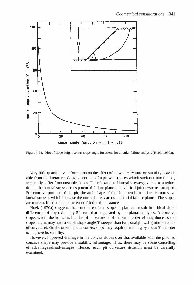
Geometrical considerations 341
Figure 4.68. Plot of slope height versus slope angle functions for circular failure analysis (Hoek, 1970a).
Very little quantitative information on the effect of pit wall curvature on stability is avail-able from the literature. Convex portions of a pit wall (noses which stick out into the pit)frequently suffer from unstable slopes. The relaxation of lateral stresses give rise to a reduc-tion in the normal stress across potential failure planes and vertical joint systems can open.For concave portions of the pit, the arch shape of the slope tends to induce compressivelateral stresses which increase the normal stress across potential failure planes. The slopesare more stable due to the increased frictional resistance.
Hoek (1970a) suggests that curvature of the slope in plan can result in critical slopedifferences of approximately 5◦ from that suggested by the planar analyses. A concaveslope, where the horizontal radius of curvature is of the same order of magnitude as theslope height, may have a stable slope angle 5◦ steeper than for a straight wall (infinite radiusof curvature). On the other hand, a convex slope may require flattening by about 5◦ in orderto improve its stability.
However, improved drainage in the convex slopes over that available with the pinchedconcave shape may provide a stability advantage. Thus, there may be some cancellingof advantages/disadvantages. Hence, each pit curvature situation must be carefullyexamined.

342 Open pit mine planning and design: Fundamentals
Figure 4.69. Slope design chart for circular failure including various safety factors (Hoek, 1970a).
4.6.6 Slope stability data presentation
Figure 4.72 developed by Hoek & Bray (1977) is a good example of how structural geologyinformation and preliminary evaluation of slope stability of a proposed open pit mine canbe presented. A contour plan of the proposed open pit mine is developed and contouredstereoplots of available structural data are superimposed. In this particular case two dis-tinct structural regions denoted by A and B have been identified and marked on the plan.Based simply on geometry (of the pit slopes and structures), the potential failure typesare identified. Each of these would then be examined using appropriate material propertiesand ground water conditions. Required design changes, additional data collection, etc. willemerge.

Geometrical considerations
Figure 4.70. Slope angle and slope height functions for different water and tension crack conditions (Hoek,1970a).
4.6.7 Slope analysis example
Reed (1983) has reported the results of applying the Hoek & Bray (1977) approach to theAfton copper-gold mine located in the southern interior of British Columbia. For the purposeof analyzing the stability of the walls of the open pit, it was divided into 9 structural domains(Fig. 4.73).
For each structural domain, a stability analysis was made of:– the relative frequency of the various fault and bedding plane orientations, and– the orientation of the pit wall in that particular domain.
343

344 Open pit mine planning and design: Fundamentals
Figure 4.71. Influence of three-dimensional pit shape upon slope stability (Hoek, 1970a).
The safety factors were calculated for plane failure, wedge failure and circular failure ineach domain. Table 4.5 shows the results of these stability analyses.
The ‘maximum safe slope angle’for the pit wall in each domain corresponds to a calculatedsafety factor of 1.2. The results in Table 4.5 predict wall failure in all domains if the slopes arewet. The mine, however, lies in a semi-arid area and expected ground water quantities weresmall. In addition, horizontal drainholes would be used to reduce ground water pressuresin domains 3 and 6. Problems would still be expected in domains 3 and 6. Since domain 3is a relatively narrow domain and the probability of a major slide occurring was small, thedesign slope of the wall in that area was not flattened. At the time the paper was written(1983), the pit had reached a depth of 480 ft. Two failures had been experienced in domain 3and several berm failures in domain 6. There was no indication of impending major failures.Final pit depth was planned to be 800 ft.
4.6.8 Economic aspects of final slope angles
Figure 4.74 illustrates the volume contained in a conical pit as a function of final slope angleand depth.
For a depth of 500 ft and an overall final pit angle of 45◦, 1.4 × 10⁷ tons of rock mustbe moved. Within the range of possible slopes (20◦ to 70◦) at this depth the volume to be

Geometrical considerations 34
Potentialplane failures
Potential wedge failures
Potentialtoppling
Stable Proposed pitbottom
STRUCTURAL REGION A
STRUCTURAL REGION B
A1
N
N
N
N
N
N
A1
B1
B1
B1
B1
B2
B2
B2
A1
A1
A1
A2
A2
A2
A2
A2
A1
A3
A3
A3
A3
A3
A3
Figure 4.72. Presentation of structural geology information and preliminary evaluation of slope stability ofa proposed open pit mine (Hoek & Bray, 1977).
moved approximately doubles for every 10◦ flattening of the slope. Flattening the slope ofthe 500 ft deep conical pit from 50◦ to 40◦ increases the mass of rock from 1.0 × 10⁷ to2.0 × 107 tons. This simple example shows that the selection of a particular slope can have asignificant impact on the scale of operations and depending upon the shape, size and gradeof the ore contained within the pit, on the overall economics.
5

346 Open pit mine planning and design: Fundamentals
Figure 4.73. Division of the Afton open pit into 9 structural domains (Reed, 1983).
Table 4.5. Calculated and design slope angles for the Aftonmine (Reed, 1983).
Domain Maximum safe slope angle Design slope angle
Wet Dry
1 24◦ 54◦ 45◦2 52◦ 52◦ 45◦3 24◦ 41◦ 45◦4A 27◦ 49◦ 45◦4B 45◦ 42◦ 45◦5 22◦ 42◦ 45◦6 28◦ 39◦ 40◦7 33◦ 42◦ 40◦8 32◦ 43◦ 40◦
4.7 PLAN REPRESENTATION OF BENCH GEOMETRY
Figure 4.75 is a cross-sectional representation of an open pit mine. Figure 4.76 is a‘birds-eye’ (plan) view of the same pit. No attempt has been made to distinguish betweenthe toes and crests (which are marked in Fig. 4.77) and hence the figure is difficult tointerpret.
Several different techniques are used by the various mines to assist in plan representationand visualization. In Figure 4.78 the bank slopes have been shaded and the benches labelledwith their elevations.

Geometrical considerations 3
Figure 4.74. Influence of pit depth and slope angle on the amount of rock removed in mining a conical openpit (Hoek & Pentz, 1970).
Figure 4.79 is an example of this type of representation for an actual mine. An alternativeis to draw the crests with solid lines and the toes with dashed lines. The result is shown indiagrammatic form in Figure 4.80 and for an actual property in Figure 4.81. Note that thebanks have also been shaded. This is however seldom done. This system of identifying toesand crests is recommended by the authors.
Some companies use the opposite system labelling the crests with dashed lines and thetoes by solid lines (Fig. 4.82). The Berkeley pit shown in Figure 4.83 is one such examplewhere this system has been applied.
If there are a great number of benches and the scale is large, there can be difficulties inrepresenting both the toes and the crests. Knowing the bench height and the bench face angle
47

348 Open pit mine planning and design: Fundamentals
Figure 4.75. Cross-section through an openpit mine.
Figure 4.76. Plan view through the portionof the pit shown in cross-section in Figure4.75 (toes and crests depicted by solid lines).
Figure 4.77. Cross-section through aportion of an open pit with toes and crestslabelled.
it is a simple matter to construct, if needed, the toes presuming that the crests are given orvice versa. Hence only one set of lines (crests or toes) is actually needed. When only oneline is used to represent a bench, the most common technique is to draw the median (midbench) elevation line at its plan location on the bench face. This is shown in section andplan in Figures 4.84 and 4.85, respectively.

Geometrical considerations 349
Figure 4.78. Plan view with the benchfaces shaded and the flat segment elevationslabelled.
6000
6150Bench elev.6185Bench elev.
6145
Bench elev.6105
Bench elev.6065
Pit limitsurface ground
line
64.6
+8% Ramp
Ramp
Level roadLevel road
Level road
Level road
Leve
l roa
d
Level road
Hoist house
+8%
+8%
+8% -8%
+8%
- 6%
Ramp
Ramp
Benc
h el
ev. 6
265
DUMP elev.6185
Main
serviceroad
Ski
pway
Changehouse
Mine office
(Contour intervel-50 ft.)
Dump elev.
6065
Ore stock pile
-4%
+4%
+4%
-8%
+8%
+8%
-5%
+8%
5750
5600
Orestockpile
Figure 4.79. Example of slope surface shading described in Figure 4.78 (Ramsey, 1944).

350 Open pit mine planning and design: Fundamentals
Figure 4.80. Plan view of a portion of the open pit (crests are denoted by solid lines and toes by dashedlines).
An actual example of its use is given in Figure 4.86. An enlarged view of a section ofthe pit is shown in Figure 4.87. The elevation label is located half way between the mediancontour lines. This is the actual location for this elevation and corresponds to the benchelevation at that point.
It is a relatively simple matter to go from median lines to actual bench representation (toesand crests) and vice versa. This process is depicted in Figure 4.88. The median contour linein the center will be replaced by the toe-crest equivalent. The road is 100 ft wide and hasa grade of 10%. The bench height is 40 ft, the bank width is 30 ft and the width of thesafety bench is 50 ft. The process begins by adding the center lines halfway to the nextcontour lines (Fig. 4.88b). Toe and crest lines are added (Fig. 4.88c) and the edge of roadis drawn (Fig. 4.88d). Finally the construction lines are removed (Fig. 4.88e). The readeris encouraged to try this construction going back and forth from toes and crests to medianlines.
4.8 ADDITION OF A ROAD
4.8.1 Introduction
Roads are one of the more important aspects of open pit planning. Their presence shouldbe included early in the planning process since they can significantly affect the slope anglesand the slope angles chosen have a significant effect on the reserves. Most of the currentlyavailable computerized pit generating techniques discussed in the following chapter do noteasily accommodate the inclusion of roads. The overall slope angles without the roadsmay be used in the preliminary designs. Their later introduction can mean large amountsof unplanned stripping or the sterilization of some planned reserves. On the other hand aflatter slope angle can be used which includes the road. This may be overly conservativeand include more waste than necessary.

Geometrical considerations 351
Figure 4.81. Example of the mapping procedure described in Figure 4.80 (Hardwick & Stover, 1960).

352 Open pit mine planning and design: Fundamentals
Figure 4.82. Plan view of a portion of the open pit (crests denoted by dashed lines and toes by solid lines).
5833
5800
5733
5667
5633
RAMP
5600
RAMP
5675
5600
5550
MP
+7%
5500
5600
5550LEGEND
CrestToeBench limitHaulage road
HER
RAMP
5500
RAMP
5433
5400 5383
5525
RAMP
5550
RAMP
+7%
5450
5500
5550
5383
5367
RA
MP
5400
RA
MP
RA
MP
54335500
5400
5633
5550
RAMP
5529
+7%
5467
Ramp
5433
5500
5433
BERKELEYSHAFT
5525
5550
Figure 4.83. Example of the mapping procedure described in Figure 4.82 (McWilliams, 1959).

Geometrical considerations 353
Figure 4.84. Procedure of denoting the median midbench elevation line on the bench face.
Figure 4.85. Resulting plan view corresponding to the midbench representation of Figure 4.84. The givenelevations are bench toe elevations.
Until rather recently, rail haulage was a major factor in open pit operations. Because of thedifficulties with sharp turns and steep grades, a great deal of time was spent by mine plannersin dealing with track layout and design. Rubber tired haulage equipment has presentedgreat flexibility and ability to overcome many difficulties resulting from inadequate or poorplanning in today’s pits. However as pits become deeper and the pressure for cost cuttingcontinues, this often neglected area will once again be in focus.
There are a number of important questions which must be answered when siting the roads(Couzens, 1979).
1. The first decision to be taken is where the road exit or exits from the pit wall will be.This is dependent upon the crusher location and the dump points.

354 Open pit mine planning and design: Fundamentals
Figure 4.86. Example mining plan composite map based on midbench contours (Couzens, 1979).
2. Should there be more than one means of access? This allows certain flexibility ofoperation but the cost of added stripping can be high.
3. Should the roads be external or internal to the pit? Should they be temporary orsemi-permanent?

Geometrical considerations 355
Figure 4.87. An enlarged portion of Figure4.86 (Couzens, 1979).
a. Road Depicted Using Median Lines
eor
eor
eor
eor
eor
edge of road (eor)
400 ft
400 ft
A
A'
400 ft100 ft
50 ft
50 ft
median line
b. The Centerlines Are Added
c. The Toe and Crest lines Are Added at a Distance of 15 ft From the MedianLines (bank width = 30 ft bank height = 40 ft)
CL
C
C
C
CL
15 ft15 ft
T
T
d. The Edge of Road Lines Are Added Connecting The Centerline Positions
e. The Extraneous Construction Lines Are Removed
median lines
median lines
crest
crest
toe
toe
Figure 4.88. Going from midbench contours to a toe and crest representation.

356 Open pit mine planning and design: Fundamentals
4. Should the road spiral around the pit? Have switchbacks on one side? Or a combination?5. How many lanes should the road have? The general rule of thumb for 2 way traffic
is: road width ≥ 4 × truck width. Adding an extra lane to allow passing may speed up thetraffic and therefore productivity but at an increased stripping cost.
6. What should the road grade be? A number of pits operate at 10% both favorable andunfavorable to the haul. A grade of 8% is preferable since it provides more latitude inbuilding the road and fitting bench entries. That is, providing it does not cause too muchextra stripping or unduly complicate the layout.
7. What should be the direction of the traffic flow? Right hand or left hand traffic inthe pit?
8. Is trolley assist for the trucks a viable consideration? How does this influence thelayout?
This section will not try to answer these questions. The focus will be on the proce-dure through which haulroad segments can be added to pit designs. The procedures canbe done by hand or with computer assist. Once the roads have been added then vari-ous equipment performance simulators can be applied to the design for evaluating variousoptions.
4.8.2 Design of a spiral road – inside the wall
As has been discussed in Section 4.3, the addition of a road to the pit involves moving thewall either into the pit and therefore losing some material (generally ore) or outward andthereby adding some material (generally waste). This design example considers the first case(inside the original pit wall). The second case will be discussed in the following section.This pit consists of the four benches whose crests are shown in Figure 4.89. Both toes andcrests are shown in Figure 4.90. The crest-crest dimension is 60 ft, the bench height is 30 ft
Figure 4.89. The four bench pit with crests shown.

Geometrical considerations 357
and a road having a width of 90 ft and a grade of 10% is to be added to the north wall. Thebench face has an angle of 56◦.
Step 1. The design of this type of road begins at the pit bottom. For reasons to be discussedlater, the point where the ramp meets the first crest line is selected with some care. In thiscase, the ramp will continue down to lower mining levels along the north and east walls,thus point A in Figure 4.91 has been selected.
Figure 4.90. The four bench pit with toes added.
Figure 4.91. Point of ramp initiation and crest intercepts.

358 Open pit mine planning and design: Fundamentals
Step 2. The locations where the ramp meets the succeeding crests are now determined.Since the bench height H is 30 ft and the road grade G is 10%, the horizontal distance Dtravelled by a truck going up to the next level is
D = 100H
G(%)= 100 × 30
10= 300 ft
Point B on the crest of the next bench is located by measuring the 300 ft distance with aruler or by swinging the appropriate arc with a compass. Points C and D are located in asimilar way.
Step 3. The crest line segments indicating the road location will be added at right angles tothe crest lines rather than at right angles to the line of the road. Hence they have a length(Wa) which is longer than the true road width (Wt). As can be seen in Figure 4.92, the angle(�) that the road makes with the crest lines is
� = sin−1 600
300= 11.5◦
Hence the apparent road width Wa (that which is laid out), is related to the true road width by
Wa = Wt
cos �= 1.02 Wt = 1.02 × 90 = 92 ft
For most practical purposes, little error results from using
Wa∼= Wt = W
Figure 4.92. Addition of ramp width (Step 3).

Geometrical considerations 359
Lines of length W drawn perpendicular to the crest lines from points A, B, C and D havebeen added to Figure 4.93a. In addition short lines running parallel to the crest starting atthe ends of these lines have been added. Line a-a′ is one such line.
Step 4. Line a-a′ is extended towards the west end of the pit. It first runs parallel to theprevious crest line but as the pit end approaches it is curved to make a smooth transitionwith the original crest line. This is shown in Figure 4.93b. The designer has some flexibility
Figure 4.93a. Completing the new crest lines (Step 4).
Figure 4.93b. Completing the new crest lines (Step 4).

360 Open pit mine planning and design: Fundamentals
Figure 4.93c. Completing the new crest lines (Step 4).
Figure 4.94. The pit as modified by the ramp (Step 5).
on how this transition occurs. Once this decision is made then the remaining crest lines aredrawn parallel to this first one. The results are shown in Figure 4.93c.
Step 5. The extraneous lines remaining from the original design are now removed. Theresulting crest lines with the included ramp are shown in Figure 4.94.
Step 6. The ramp is extended from the crest of the lowest bench to the pit bottom. This isshown in Figure 4.95. The toe lines have been added to assist in this process. In Figure 4.95,

Geometrical considerations
EDREDR
EDR
Figure 4.95. Addition of entrance ramp and toe lines (Step 6).
the slopes have been shaded to help in the visualization. The edge of road (EOR) lines shownare also crest lines.
4.8.3 Design of a spiral ramp – outside the wall
In the previous section the addition of a spiral ramp lying inside the original pit contourswas described. It’s addition meant that some material initially scheduled for mining wouldbe left in the pit. For the case described in this section where the ramp is added outside theinitial pit shell design, additional material must be removed. The same four bench mine asdescribed earlier will be used:
Bench height = 30 ft
Crest-crest distance = 60 ft
Road width = 90 ft
Road grade = 10%
Bench slope angle = 56◦
Step 1. The design process begins with the crest of the uppermost bench. A decision must bemade regarding the entrance point for the ramp as well as direction. As shown in Figure 4.96,the entrance should be at point A in the direction shown. Mill and dump locations are primefactors in selecting the ramp entrance point. From this point an arc of length L equal to theplan projection of the ramp length between benches is struck. This locates point B. Frompoint B an arc of length L is struck locating point C, etc.
Step 2. From each of the intersection points A, B, C and D, lines of length Wa (appar-ent road width) are constructed normal to their respective crest lines. This is shown in
361

362 Open pit mine planning and design: Fundamentals
Ramp Direction
AL B
C
D
Figure 4.96. Point of ramp initiation and crest intercepts (Step 1).
AWa
Wa
Wa
Wa
B
C
D
Figure 4.97. Addition of ramp width (Step 2).
Figure 4.97. A short length of line is drawn parallel to the crest line from the end in the rampdirection.
Step 3. Beginning with the lowermost crest, a smooth curve is drawn connecting the newcrest with the old. This is shown in Figure 4.98.

Geometrical considerations 363
A Wa
Wa
Wa
Wa
B
C
D
Figure 4.98. Drawing the new crest lines (Steps 3 and 4).
AB
C
D
Figure 4.99. The pit as modified by the ramp (Step 5).
Step 4. The remaining new crest line portions are drawn parallel to the first crest workingupwards from the lowest bench.
Step 5. The extraneous lines are removed from the design (Fig. 4.99).
Step 6. The toe lines at least for the lowest bench are added and the ramp to the pit bottomadded. In Figure 4.100, the slopes have been shaded to assist in viewing the ramp.

364 Open pit mine planning and design: Fundamentals
AB
C
D
Figure 4.100. Addition of entrance ramp and toe lines (Step 6).
4.8.4 Design of a switchback
In laying out roads the question as to whether to:(a) spiral the road around the pit,(b) have a number of switchbacks on one side of the pit, or(c) use some combination.
Generally (Couzens, 1979) it is desirable to avoid the use of switchbacks in a pit.Switchbacks:
– tend to slow down traffic,– cause greater tire wear,– cause various maintenance problems,– probably pose more of a safety hazard than do spiral roads (vision problems, machinery
handling, etc.).Sometimes the conditions are such that switchbacks become interesting:– when there is a gently sloping ore contact which provides room to work in switchbacks
at little stripping cost;– it may be better to have some switchbacks on the low side of the pit rather than to accept
a lot of stripping on the high side.The planner must take advantage of such things. The general axiom should be to design
the pit to fit the shape of the deposit rather than vice versa. If switchbacks are necessary theplanner should:
– leave enough length at the switchbacks for a flat area at the turns so that trucks don’thave to operate on extremely steep grades at the inside of curves,
– consider the direction of traffic,– consider problems the drivers may have with visibility,– consider the effect of weather conditions on the design (ice, heavy rain, etc.).

Geometrical considerations 365
Figure 4.101. The starter pit for switchback addition to the north wall (Step 1).
In this section the steps required to add a switchback to the pit shown in Figure 4.89 willbe described. The switchback will occur between the second and third benches on the northpit wall.
Step 1. The design will begin from the pit bottom. In this case the ramp moves into theas-designed pit wall. Figure 4.101 shows the modified pit with the crest lines drawn forbenches 4 (lowermost) and 3. This is the same procedure as with the spiral ramp. The benchheight has been selected as 30 ft and the road gradient is 10%. Hence the plan distance R is300 ft.
Step 2. The center C used to construct the switchback is now located as shown in Fig-ure 4.102. There are three distances involved L1, L2 and L3. L2 is the given crest-crestdistance. Distances L1 and L3 must now be selected so that
L1 + L3 = R − L2
In this particular case L1 = 0.5R = 150 ft. Since L2 = 60 ft, then L3 = 90 ft. The center C islocated at L2/2 = 30 ft from the 3 construction lines. A vertical line corresponding to roadwidth W is drawn at the end of L3.
Step 3. In Figure 4.103 the curve with radius R2 = L2/2 is drawn from C. This becomesthe inner road radius. It should be compared with the turning radius for the trucks beingused. A second radius R3 = 2W is also drawn from C. The intersection of this curve with thehorizontal line drawn from C becomes a point on the bench 2 crest. It is noted that actualdesigns may use values of R3 different from that recommended here. This is a typical value.Portions of the bench 2 crest lines have been added at the appropriate distances.
Step 4. A smooth curve is now added going from line a − b through crest point CP to linec − d. The designer can use some judgement regarding the shape of this transition line.
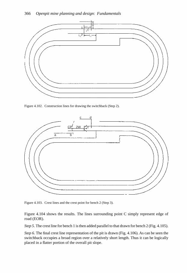
366 Open pit mine planning and design: Fundamentals
wL3
L1L2
C+
Figure 4.102. Construction lines for drawing the switchback (Step 2).
a b
CP 2W
c
c
d
Figure 4.103. Crest lines and the crest point for bench 2 (Step 3).
Figure 4.104 shows the results. The lines surrounding point C simply represent edge ofroad (EOR).
Step 5. The crest line for bench 1 is then added parallel to that drawn for bench 2 (Fig. 4.105).
Step 6. The final crest line representation of the pit is drawn (Fig. 4.106). As can be seen theswitchback occupies a broad region over a relatively short length. Thus it can be logicallyplaced in a flatter portion of the overall pit slope.

Geometrical considerations 367
2W c
Figure 4.104. The transition curve has been added (Step 4).
+c
Figure 4.105. The crest line for bench 1 is added (Step 5).
Step 7. The toes are drawn and the lower section of the ramp (between bench 4 crest andthe pit floor) added (Fig. 4.107).
Two examples of switchbacks are shown in Figure 4.108.
4.8.5 The volume represented by a road
The addition of a haulroad to a pit results in a large volume of extra material which must beremoved or a similar volume in the pit which is sterilized (covered by the road). Thus even

368 Open pit mine planning and design: Fundamentals
Figure 4.106. The final pit crest lines with the switchback (Step 6).
Figure 4.107. The lower entrance ramp and the toes are added (Step 7).
though production flexibility can be improved and the security of having several accessesto the pit can lead to other savings such as steeper interramp slopes, the additional haulroads are associated with significant expense. To demonstrate this, consider the pit shownin Figure 4.109 which contains no haulroad.

Geometrical considerations 369
Figure 4.108. An example showing two different switchback (520 region and 1040 region) situations(Couzens, 1979).
The same pit with the road added, is shown in Figure 4.110. The shaded regions showthe differences between sections A, B, C, D and E with and without the road.
In plan the length L of the road is
L = (No. of benches × Bench height) 100
Road grade (%)= 4 × 30 × 100
10= 1200 ft (4.4)
Because the road is oriented at angle � to the pit axis, the length projected along the axis is
L2 = L cos � = 1176 ft (4.5)
The sections are made normal to this axis. They are spaced every 294 ft.The road areas for each section are shown in Figure 4.111. The shaded boxes are of the
same area
A = WA × Bench height

370 Open pit mine planning and design: Fundamentals
Figure 4.109. Plan and section views of a four bench pit without ramp.
They can be lined up as shown in Figure 4.111a. These in turn can be plotted such as shownin Figure 4.111b.
The volume contained in the ramp is that of a triangular solid of width WA, length L2 andheight varying linearly from 0 to the pit depth (Fig. 4.112). This can be expressed as
V = 1
2WAL2 × Pit depth = 1
2WAL cos � × Pit depth (4.6)
which can be simplified to
V = 1
2WA
(Pit depth)2
Grade (% )100 cos � (4.7)
Since the apparent road width WA is equal to
WA = Wt
cos �
The simplified road volume formula becomes
V = 1
2
100 × (Pit depth)2
Grade (%)WT (4.8)

Geometrical considerations
Figure 4.110. Plan and section views of a four bench pit with ramp.
In the present case the volume is
V = 1
2
100
10(120)2 × 90 = 6, 480, 00 ft3 = 240, 000 yd3
For a tonnage factor of 12.5 ft3/st, there are 518,400 st involved in the road.The overall length of the road (Lov) is given by
Lov =√
L2 + (Pit depth)2 (4.9)
371

Open pit mine planning and design: Fundamentals
a. b.
Figure 4.111. Construction to show road volume on each section.
Figure 4.112. The volume involved in the ramp.
In this case it is
Lov =√
(1200)2 + (120)2 = 1206 ft
4.9 ROAD CONSTRUCTION
4.9.1 Introduction
Good haulroads are a key to successful surface mining operations. Poorly designed, con-structed and maintained roads are major contributors to high haulage costs and pose safetyhazards. In this section some of the basic design aspects will be discussed. Figure 4.113shows a typical cross section through a road.
372

Geometrical considerations 373
Figure 4.113. Simplified flexible pavement structure (Seelye, 1945).
Generally there are four different layers involved:– subgrade,– subbase,– base,– wearing surface.
The subgrade is the foundation layer. It is the structure which must eventually support allthe loads which come onto the wearing surface. In some cases this layer will simply be thenatural earth surface. In other and more usual instances, it will be the compacted rock orsoil existing in a cut section or the upper layer of an embankment section.
The wearing surface provides traction, reduces tractive resistance, resists abrasion, ravel-ling and shear, transmits tire load to the base and seals the base against penetration of surfacewater. Although this surface may be asphalt or concrete, most typically it is crushed rock.
The base is a layer of very high stability and density. It’s principal purpose is to distributeor ‘spread’ the stresses created by wheel loads acting on the wearing surface, so that theywill not result in excessive deformation or the displacement of the subgrade. In additionit insulates the subgrade from frost penetration and protects the working surface from anyvolume change, expansion and softening of the subgrade.
The subbase which lies between the base and subgrade, may or may not be present. Itis used over extremely weak subgrade soils or in areas subject to severe frost action. Theymay also be used in the interest of economy when suitable subbase materials are cheaperthan base materials of a higher quality. Generally the subbase consists of a clean, granularmaterial. The subbase provides drainage, resists frost heave, resists shrinkage and swellingof the subgrade, increases the structural support and distributes the load.
4.9.2 Road section design
In designing the road section, one begins with the maximum weight of the haulage equipmentwhich will use the road. To be as specific as possible, assume that the haulage trucks havea maximum gross vehicle weight of 200,000 lbs including their 58 st payload. The load isdistributed as follows:
– 33% on the front tires, and– 67% on the dual rear tires.
The load on each of the front tires is 33,000 lbs. For each of the four rear tires (2 sets ofduals) the load is 33,500 lbs. Thus the maximum loading to the wear surface is applied by

374 Open pit mine planning and design: Fundamentals
Figure 4.114. Load distribution beneath a tire (Seelye, 1945).
the rear tires. Although the contact pressure between the wheel and the road depends onthe tire inflation pressure and the stiffness of the tire side walls, for practical purposes, thecontact pressure is assumed to be equal to the tire pressure. Since for this truck, the inflationpressure is about 90 psi, the bearing pressure on the road surface is 90 psi or 12,960 psf. Inlieu of knowing or assuming an inflation pressure, Kaufman & Ault (1977), suggest that avalue of 16,000 psf (110 psi), will rarely be exceeded. The tire contact area is
Contact area (in2) = Tire load (lbs)
Tire inflation pressure (psi)(4.10)
For the rear tires
Contact area (in2) = 33,500
90= 372 inch2
Although the true contact area is approximately elliptical, often for simplicity the contactarea is considered to be circular in shape. The contact pressure is usually assumed to beuniformly distributed. Because
πr2 = 372 inch2
the radius of the tire contact area is
r ∼= 11 inch
and the average applied pressure is 90 psi (12,960 psf). As one moves down, away fromthe road surface, the force of the tire is spread over an ever increasing area and the bearingpressure is reduced. For simplicity, this load ‘spreading’ is assumed to occur at 45◦. Thisis shown in Figure 4.114. Thus at a depth of 10 inches beneath the tire, the pressure radiuswould have increased to 21 inches and the pressure has dropped to 24.7 psi (3560 psf).However, for this truck there are dual rear wheels. Tire width is about 22 inches and thecenterline spacing for the tires in each set is about 27 inches. This is shown diagrammaticallyin Figure 4.115.

Geometrical considerations
Figure 4.115. Load interaction with dual wheels.
As can be seen, the bearing pressure bulbs from each tire overlap. The greatesteffect is observed along the line separating the tires. This interaction changes with tirewidth, tire separation and depth below the wear surface. To take this into account,Kaufman & Ault (1977) suggest using an equivalent single tire wheel load (LE) whichis 20% higher than the single tire load (LT ). Thus,
LE = 1.20 × LT (4.11)
In the case of the 58 st capacity truck
LE = 1.20 × 33, 500 ∼= 40, 000 lb
The combined subbase, base and wearing surface thickness must be sufficiently large sothat the stresses occurring in the subgrade will not cause excessive distortion or displacementof the subgrade soil layer.
As a first guide, one can compare the required wear surface pressure to the bearing capacityof various subgrade materials. These are given in Table 4.6.
As can be seen, any subgrade that is less consolidated than soft rock will require additionalmaterial in order to establish a stable base. If, for example, the subgrade is a compact sand-clay soil with a bearing capacity of 6000 psf, then base/subbase materials of suitable strengthwould have to be placed down to increase the distance between the wear surface and thesubgrade. Using the approach described earlier
π(11 + t)2 × 6000 = π(11)2 × 12, 960
375

376 Open pit mine planning and design: Fundamentals
Table 4.6. Bearing capacities of subgrade materials (Kaufman & Ault, 1977).
Material 1000 psf
Hard, sound rock 120Medium hard rock 80Hard pan overlying rock 24Compact gravel and boulder-gravel formations; very compact sandy gravel 20Soft rock 16Loose gravel and sandy gravel; compact sand and gravelly sand; 12
very compact sand – inorganic silt soilsHard dry consolidated clay 10Loose coarse to medium sand; medium compact fine sand 8Compact sand-clay soils 6Loose fine sand; medium compact sand – inorganic silt soils 4Firm or stiff clay 3Loose saturated sand clay soils, medium soft clay 2
the minimal required thickness (t) would be
t ∼= 5 inch
The technique often applied to determine the working surface, base and subbase thicknessesinvolves the use of California bearing ratio (CBR) curves. The CBR test is an empiricaltechnique for determining the relative bearing capacity of the aggregate materials involvedin road construction. In this test the aggregate material with a maximum size of 3/4 inch isplaced in a 6 in diameter metal mold. The material is compacted by repeatedly dropping a10 lb weight through a height of 18 in. After compaction, a cylindrical piston having an endarea of 3 inch2 is pushed into the surface at a rate of 0.05 inch/minutes. The CBR is calculatedby dividing the piston pressure at 0.1 or 0.2 inch penetration by reference values of 1000 psifor 0.1 inch and 1500 psi for 0.2 inch. These standard values represent the pressures observedfor a high quality, well graded crushed stone reference material. The calculated pressureratios are multiplied by 100 to give the CBR value expressed as a percent. Figure 4.116shows design curves based upon the use of CBR values. The subbase thickness has beenplotted against CBR/soil type for various wheel loads.
To demonstrate the use of these curves, consider the 58-st capacity truck travelling overa haulroad which the subgrade material is a silty clay of medium plasticity (CBR = 5). Onefinds the intersection of CBR = 5 and the 40,000 lb equivalent single wheel load. Movinghorizontally it is found that the required distance between the wear surface and the subgrademust be a minimum of 28 inches.
Fairly clean sand with a CBR of 15 is available to serve as subbase material. Repeat-ing the process, one finds that this must be kept 14 inches away from the wear surface.The base material is well graded, crushed rock with a CBR rating of 80. The intersectionof the 40,000 lb curve and CBR = 80 occurs at 6 inches. This 6 inch gap between the topof the base and the wear surface is intended to accommodate the wear surface thickness. Ifthe actual wear surface is thinner than this, the remaining space is simply added to the basethickness (CBR equal to at least 80). Figure 4.117 shows the final results (Kaufman & Ault,1977).
In most open pit mines, the wear surface is formed by well graded, crushed rock with amaximum dimension smaller than that used as base. Since traffic loading is directly applied

Geometrical considerations 377
Figure 4.116. CBR curves (Kaufman & Ault, 1977).
to the aggregate layer, the upper most aggregate layer must possess sufficient strength andrutting resistance to minimize both
– bearing capacity failure, and– rutting failure
within the layer.The aggregate layer must also possess good wear resistance to minimize attrition under
traffic. Table 4.7 indicates an acceptable aggregate size distribution (gradation) for thiswearing surface.
Particle gradation is the distribution of the various particle size fractions in the aggregate.A well graded aggregate has a good representation of all particle size fractions from themaximum size through the smaller sizes. This is needed so that particles lock togetherforming a dense, compact surface. The opposite of a well graded aggregate is one whichis poorly graded. Here the particles are all about the same size. Such a distribution might
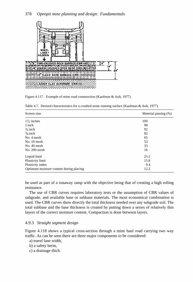
378 Open pit mine planning and design: Fundamentals
Figure 4.117. Example of mine road construction (Kaufman & Ault, 1977).
Table 4.7. Desired characteristics for a crushed stone running surface (Kaufman & Ault, 1977).
Screen size Material passing (%)
11/2 inches 1001 inch 983/4 inch 923/8 inch 82No. 4 mesh 65No. 10 mesh 53No. 40 mesh 33No. 200 mesh 16
Liquid limit 25.2Plasticity limit 15.8Plasticity index 9.4Optimum moisture content during placing 12.2
be used as part of a runaway ramp with the objective being that of creating a high rollingresistance.
The use of CBR curves requires laboratory tests or the assumption of CBR values ofsubgrade, and available base or subbase materials. The most economical combination isused. The CBR curves show directly the total thickness needed over any subgrade soil. Thetotal subbase and the base thickness is created by putting down a series of relatively thinlayers of the correct moisture content. Compaction is done between layers.
4.9.3 Straight segment design
Figure 4.118 shows a typical cross-section through a mine haul road carrying two waytraffic. As can be seen there are three major components to be considered:
a) travel lane width,b) a safety berm,c) a drainage ditch.

Geometrical considerations 379
Figure 4.118. Typical design haulroad width for two-way traffic using 85 st capacity trucks (Couzens, 1979).
Figure 4.119. Multi-lane road design widths (Kaufman & Ault, 1977).
The width of each is added together to obtain the total roadway width.The width criteria for the traveled lane of a straight haul segment should be based on the
widest vehicle in use.The 1965 AASHO Manual for Rural Highway Design recommends that each lane of travel
should provide clearance to the left and right equal to one-half of the vehicle width. This isshown in Figure 4.126 for a 12-ft wide truck.
Values for other truck widths are given in Table 4.8. Typical widths of haulage trucksused in open pit mines are listed in Table 4.9.
For the two-way traffic which is most common in open pit mines, the rule of thumb isthat roadway width should be no less than four times the truck width (Couzens, 1979):
Roadway width ≥ 4 × Truck width (4.12)

380 Open pit mine planning and design: Fundamentals
Table 4.8. Recommended lane widths for tangent sections (Kaufman & Ault, 1977).
Vehicle width (ft) 1 lane 2 lanes 3 lanes
8 16 28.0 409 18 31.5 45
10 20 35.0 5011 22 38.15 5512 24 42.0 6013 26 45.5 6514 28 49.0 7015 30 52.5 7516 32 56.0 8017 34 59.5 8518 36 63.0 9019 38 66.5 9520 40 70.0 10021 42 73.5 10522 44 77.0 11023 46 80.5 11524 48 84.0 12025 50 87.5 12526 52 91.0 13027 54 94.5 13528 56 98.0 140
Table 4.9. Widths for various size rear dump trucks (this width includesthe safety berm).
Truck size Approx. width 4 × width Design width(m) (m)
m ft
35 st 3.7 14.8 15 5085 st 5.4 21.6 23 75
120 st 5.9 23.6 25 85170 st 6.4 25.6 30 100
Some mines have two lanes of traffic in one direction to allow passing for loaded uphilltraffic. The downhill empty traffic travels in a single lane. A rule of thumb for the width ofsuch a three lane road is 5 times the truck width.
The steps to be followed in selecting a design width are (Kaufman & Ault, 1977):1. Define the width of all equipment that may have to travel the haulage road.2. Solicit dimensional data for any anticipated new machines.3. Determine the overall width of any equipment combinations that may be involved in a
passing situation.4. Delineate the location of road segments requiring a greater than normal width.
There may be wider stretches of road where there is merging of traffic streams such as neara crusher. Curves and switchbacks require special consideration. These will be discussedlater.

Geometrical considerations 381
Figure 4.120. Cross slope design.
Table 4.10. Design widths (ft) for curves – single unit vehicles (Kaufman & Ault, 1977).
Radius (R) on One-lane haulageway, Two-lane haulageway, Three-lane haulageway,inner edge of vehicle category vehicle category vehicle categorypavement (ft)
1 2 3 4 1 2 3 4 1 2 3 4
Minimum 29 34 45 70 51 60 79 123 73 86 113 17625 27 34 44 68 48 60 76 119 68 86 109 17050 25 31 41 63 44 54 72 110 63 77 103 158
100 24 29 39 59 42 51 69 103 60 73 99 147150 24 29 39 58 41 50 68 101 59 72 97 145200 23 29 38 57 41 50 67 101 59 712 96 144Tangent 23 28 37 56 40 48 65 98 57 69 93 140
The road surface is often slightly crowned such as shown in Figure 4.120, to facilitatewater runoff. The cross slope is expressed in inches per foot of width. Most mine roads areconstructed of gravel and crushed rock. In this case, except where ice/mud is a problem, thecross slope should be 1/2 inch per foot (0.04 ft/ft). For relatively smooth road surfaces suchas asphaltic concrete which can rapidly shed water or roads which have ice/mud problems,a cross slope of 1/4 inch per foot (0.02 ft/ft) is appropriate.
For single lanes, it is necessary to decide whether the left edge should be higher than theright or vice-versa. For three-lane surfaces, there should be a continuous cross slope for thetwo lanes having traffic in the same direction. It should be noted that the use of a cross-slopeincreases the steering effort by the driver. Thus there must be a balance between steerabilityand water drainage.
4.9.4 Curve design
For straight sections it was recommended that the left and right vehicle clearances shouldbe half of the vehicle width. In the case of curves this distance must be increased both dueto vehicle overhang and increased driving difficulty.
Tables 4.10 and 4.11 provide the design widths as a function of the inner pavementradius for various combinations of vehicle size, vehicle type and roadway types. For
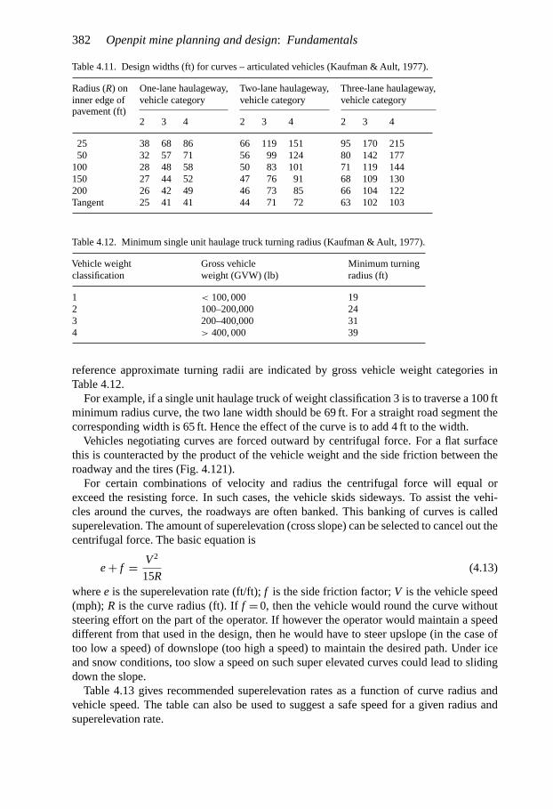
382 Open pit mine planning and design: Fundamentals
Table 4.11. Design widths (ft) for curves – articulated vehicles (Kaufman & Ault, 1977).
Radius (R) on One-lane haulageway, Two-lane haulageway, Three-lane haulageway,inner edge of vehicle category vehicle category vehicle categorypavement (ft)
2 3 4 2 3 4 2 3 4
25 38 68 86 66 119 151 95 170 21550 32 57 71 56 99 124 80 142 177
100 28 48 58 50 83 101 71 119 144150 27 44 52 47 76 91 68 109 130200 26 42 49 46 73 85 66 104 122Tangent 25 41 41 44 71 72 63 102 103
Table 4.12. Minimum single unit haulage truck turning radius (Kaufman & Ault, 1977).
Vehicle weight Gross vehicle Minimum turningclassification weight (GVW) (lb) radius (ft)
1 < 100, 000 192 100–200,000 243 200–400,000 314 > 400, 000 39
reference approximate turning radii are indicated by gross vehicle weight categories inTable 4.12.
For example, if a single unit haulage truck of weight classification 3 is to traverse a 100 ftminimum radius curve, the two lane width should be 69 ft. For a straight road segment thecorresponding width is 65 ft. Hence the effect of the curve is to add 4 ft to the width.
Vehicles negotiating curves are forced outward by centrifugal force. For a flat surfacethis is counteracted by the product of the vehicle weight and the side friction between theroadway and the tires (Fig. 4.121).
For certain combinations of velocity and radius the centrifugal force will equal orexceed the resisting force. In such cases, the vehicle skids sideways. To assist the vehi-cles around the curves, the roadways are often banked. This banking of curves is calledsuperelevation. The amount of superelevation (cross slope) can be selected to cancel out thecentrifugal force. The basic equation is
e + f = V 2
15R(4.13)
where e is the superelevation rate (ft/ft); f is the side friction factor; V is the vehicle speed(mph); R is the curve radius (ft). If f = 0, then the vehicle would round the curve withoutsteering effort on the part of the operator. If however the operator would maintain a speeddifferent from that used in the design, then he would have to steer upslope (in the case oftoo low a speed) of downslope (too high a speed) to maintain the desired path. Under iceand snow conditions, too slow a speed on such super elevated curves could lead to slidingdown the slope.
Table 4.13 gives recommended superelevation rates as a function of curve radius andvehicle speed. The table can also be used to suggest a safe speed for a given radius andsuperelevation rate.

Geometrical considerations 383
Figure 4.121. Centrifugal force effects oncurves.
Table 4.13. Recommended superelevation rates (feet per footof width) (Kaufman & Ault, 1977).
Radius of Speed of vehicle (mph)curve (ft)
10 15 20 25 30 35 and over
50 0.04 0.04100 0.04 0.04 0.04150 0.04 0.04 0.04 0.05250 0.04 0.04 0.04 0.04 0.06300 0.04 0.04 0.04 0.04 0.05 0.06600 0.04 0.04 0.04 0.04 0.04 0.05
1000 0.04 0.04 0.04 0.04 0.04 0.04
Table 4.14. Recommended rate of cross-slope change (Kaufman &Ault, 1977).
Vehicle speed (mph) 10 15 20 25 30 35 and above
Cross-slope change in 0.08 0.08 0.08 0.07 0.06 0.05100-ft length ofhaulageway (ft/ft)
There is a certain distance required to make the transition from the normal cross-slopesection to the superelevated portion and back again. This is called the superelevation runout.The purpose is to help ease the operator into and out of the curve. Part of the transition canbe placed in the straight (tangent) portion and part in the curve. The design criteria of 1/3 inchcurve and 2/3 inch the tangent is used here. The recommended rate of cross-slope change asa function speed is given in Table 4.14.

384 Open pit mine planning and design: Fundamentals
To illustrate the use of this table, assume a vehicle is traveling at 35 mph on tangent withnormal cross slope 0.04 ft/ft to the right. It encounters a curve to the left necessitating asuperelevation rate of 0.06 ft/ft to the left. The total cross-slope change required is 0.10 ft/ft(0.04 + 0.06). The table recommends a 0.05 ft/ft cross-slope change in 100 ft. Thus thetotal runout length is computed as 200 ft [(0.10/0.05) × 100 = 200]. One-third of this lengthshould be placed in the curve and two-thirds on the tangent.
4.9.5 Conventional parallel berm design
U.S. federal law (MSHA, 1992) contains the following guidance regarding the need forberms/guardrails in open pit mines (Section 57.9300):
(a) Berms or guardrails shall be provided and maintained on the banks of roadways wherea drop-off exists of sufficient grade or depth to cause a vehicle to overturn or endangerpersons in equipment.
(b) Berms or guardrails shall be at least mid-axle height of the largest self-propelledmobile equipment which usually travels the roadway.
(c) Berms may have openings to the extent necessary for roadway drainage.(d)Where elevated roadways are infrequently traveled and used only by service or mainte-
nance vehicles, berms or guardrails are not required (when certain very specific conditionsare met).The principal purpose of these berms is to redirect the vehicle back onto the roadway andaway from the edge. Their effectiveness in this regard is controlled by berm face angle,berm facing, the angle of incidence, and primarily by berm height. The stopping of runawayvehicles is accomplished by median berms (Subsection 4.9.6) or special escapeways. Onenegative effect of berms is the possibility of the vehicles overturning due to climbing thesides.
There are two principal berm designs in common use today. The triangular or trapezoidalshaped berm is generally formed from blasted materials. The sides stand at the angle ofrepose of the material. The second type is the boulder-faced berm. Here, large boulders,lined up along the haulage road, are backed with earthen material or blasted rock.
For the triangular berms, the design rule of thumb is that the height must be equal to orgreater than the static rolling radius (SRR) of the vehicle’s tire. For boulder-faced berms,the height of the berm should be approximately equal to the tire height. Figure 4.122 showsthe relationship between the static rolling radius and haulage vehicle carrying capacity. Tireheight (TH) is about equal to:
TH = 1.05 × 2 × SRR (4.14)
4.9.6 Median berm design
Some means should be provided on haulroads to reduce truck speed or handle the truck thatloses its brakes. This is particularly true when long, downhill loaded hauls are involved.Currently the most successful technique is through the use of median berms, also knownas ‘straddle berms’ or ‘whopper stoppers’ (Winkle, 1976a,b). These are constructed of sandor some other fine grained material. The height of these berms is designed to impinge onthe under-carriage of the truck. Since the typical distance between the road surface to theundercarriage is of the order of 2 to 3 ft for the range of available haulers, it is not necessaryto build a big barrier providing just another crash hazard.

Geometrical considerations 385
70
60
50
40
30
20
10
50 100 150 200 2500
0Haulage Truck Capacity (tons)
Sta
tic R
ollin
g R
adiu
s (I
ns)
Figure 4.122. Static rolling radius as a function of haulage truck capacity (Goodyear, 1992).
Guidance in median berm design provided by Kaufman & Ault (1977) is given in Fig-ure 4.123. The dimensions corresponding to the letters in the figure are given in Tables 4.15and 4.16. The vehicle categories are based upon gross vehicle weights.
Training the driver to get onto the berm or into the bank just as soon as they start to losecontrol of their truck and before they build up speed is as important, or more important,than the berm design itself (Couzens, 1979).
4.9.7 Haulage road gradients
A number of rules of thumb regarding haulage road gradients have been provided by Couzens(1979). These are given below:
1. In a pit where there is a considerable vertical component to the haulage requirement,the grade will have to be fairly steep to reduce the length of the road and the extra materialnecessary to provide the road length. The practical maximum grade is considered to be 10%.

386 O
pen pit mine planning and design: F
undamentals
Conventional Berm
Median BermS
Downhill
DownhillHaulage Lane
Direction of Travel
A
A
A/2
A/2
150'
150'
PLAN
C
C
Downhill Haulage
Traffic Lane
APLAN
Cut Face
S
PROFILE
SECTION A-A
1½:1slope
1½:1 slope1½:1 slope
4:1 slope
PROFILE
B
ASECTION
B
Figure 4.123. Runaway-vehicle collision berms (Kaufman & Ault, 1977)

Geometrical considerations 387
Table 4.15. Typical median berm dimensions (see Figure 4.123)(Kaufman & Ault, 1977).
A B C
Category 1 11′–12′ 3.5′–4′ 14′–16′13 to 25 st<100,000 lb
Category 2 12′–15′ 4′–5′ 16′–20′28 to 50 st100,000–200,000 lb
Category 3 15′–18′ 5′–6′ 20′–24′55 to 120 st>200,000–400,000 lb
Category 4 18′–32′ 6′–11′ 24′–44′120 to 250 st> 400,000 lb
Table 4.16. Berm spacing (S) expressed in feet assuming that the initial speed at brake failure is 10 mph.
Equivalent Maximum permissible vehicle speed or terminal speed at entrance todowngrade, (%) safety provision (mph)
15 20 25 30 35 40 45 50
1 418 1003 1755 2674 3760 5013 6433 80213 140 335 585 892 1254 1671 2145 26745 84 201 351 535 752 1003 1287 16047 60 144 251 382 537 716 919 11469 47 112 195 297 418 557 715 892
11 38 92 160 243 342 456 585 73013 33 78 135 206 290 386 495 61715 28 67 117 179 251 335 429 535
A number of pits operate quite well at 10% grades both favorable and unfavorable to theloads.
2. An 8% road grade is probably preferred providing that it does not cause too muchextra stripping or unduly complicate the road layout. This grade provides more latitude in:(a) building the road and (b) fitting in bench entries without creating some locally over-steepplaces, than do steeper grades.
3. There is normally nothing to be gained by flattening the road below 8%, unless thereis a long distance to travel without requiring much lift. The extra length on the grade andthe complications of fitting the road into the available room or doing extra stripping wouldprobably offset any increase in uphill haul speed.
4. Pit geometry is the prime consideration and roads are designed to fit the particular situation.Thus there often will be a number of different grade segments in haul roads.

388 Open pit mine planning and design: Fundamentals
4.9.8 Practical road building and maintenance tips
The preceding parts of this section have dealt with some of the general road design principles.Winkle (1976a,b) has provided a number of practical tips based upon many years of practicalexperience. Some of these have been included below.
1. The size of the orebody and the nature of the overlying topography will have considerableimpact upon road design. When the orebody is small it will likely be advantageous to stripimmediately to the projected pit limits, since some mining inefficiencies occur when miningareas overlap. This dictates an immediate final road layout on the backslope which is plannedto avoid expensive modification. For very large orebodies, particularly where an outcropof ore is exposed, it is highly unlikely that initial stripping will extend to the final plannedperimeter. Careful study of the topography is required to ensure proper rapid access. The costof rehandling material dumped within eventual pit limits must be weighed against increasedhaul distances, sharp curves, etc.
2. Change in equipment size frequently is a cause of road modification, particularly width.Pit design should incorporate allowance for reasonable future equipment size increases.
3. When mixed haulage fleets with varying speeds are used or where trucks hauling fromtwo or more shovels are using the same haul roads, passing lanes on long grades should beconsidered.
4. Short radius curves result in reduced productivity, high tire cost, high maintenancecost (particularly electric wheels) and introduce additional safety hazards into the oper-ation. Switchbacks are to be avoided unless a tradeoff of reduced stripping dictates theirconstruction.
5. When curves are necessary in haulroads, superelevation must be designed into the curves.Excessive superelevation is to be avoided since trucks rounding a curve slippery from rain,ice or overwetting can slide inward and possibly overturn. Overly ‘supered’ curves result inexcessive weight and wear on the inside tires.
6. Often curves are constructed to provide an access road into a mining bench from a steeplyinclined haul road. To prevent the inside (and lower) side of this superelevated access curvefrom being at a steeper gradient than the main haul road, it is necessary to reduce (flatten)the center line grade of the curve. The inside grade should not be allowed to exceed themain road grade.
If enough room is available, the inside gradient of the curve should in fact be flatter thanthe main road grade to compensate for the increased rolling resistance. To accomplish thisthe design of a transition spiral is necessary.
7. Curves in the flat haul portion just as the trucks are leaving the shovel are quite critical.Due to the centrifugal forces induced by the curve, spill rock is thrown to the outside. Wherepossible, the return lane should be on the inside of the curve to avoid spill falling in the pathof returning trucks and damaging tires. This can be accomplished by the use of crossoversto change traffic from right hand to left hand or vice versa in the necessary area. Adequatewarning lights must be used at night to insured the safety at the crossovers. The costs of thewarnings are small compared to savings in tire costs.

Geometrical considerations 38
8. Waste dumps should be designed for placement at a two percent upgrade. This is donefor the following reasons:
(a) The increase in dump height and volume occurs with little increase in haul speed orfuel cost. Because of the rapid dump volume increase, the haul distance is reduced.
(b) Better drainage on dumps.(c) Some additional safety is afforded drivers backing up for dumping.(d) If eventual dump leaching is planned, the water distribution is less expensive.
9. Within the mining areas, roads are built of the country rock at hand and are surfaced withthe best material available within a reasonable haul distance. In the case of using somethingother than environmental rock to surface roads within the ore zone, double handling costsas well as ore dilution must be considered.
10. Main roads into the pit are usually planned for extended time of use and will justifymore expenditure for subbase compaction and surfacing than temporary access roads.
11. If intended for use as a haul road, engineering layout should precede construction ofeven the shortest road or ramp. Mine survey crews should place desired stakes for initialcuts and fills and grade stakes including finish grade stakes.
12. When shovels are working in coarse, sharp rock faces, loading should be stoppedperiodically to allow fine material to be brought in and used to cap the surface of the loadingarea. Similar activity should be performed on waste dumps.
13. Constant attention to haul road surfaces is necessary. Soft spots, holes, ‘washboard’areas, etc. should be repaired as soon as possible. Repairs usually consist of digging out theincompetent road material and replacing it with more desirable rock.
14. Grading of roads often results in a buildup of windrows on road edges. These narrow theroads and place sharp rocks in a position to damage tire sidewalls. Windrow buildup shouldbe removed by loader or careful grader application.
15. Balding or grading of roads and dumps should be done when possible at a time whentraffic can be moved to other areas. Many tires have been damaged by trucks driving throughwindrows created by graders assigned to improve roads and thereby reduce tire costs.
16. Maintenance of haul roads is equally important to good haulage costs as are design andconstruction. As more tires are damaged in shovel pits and dump areas than on actual haulroads, cleanup around an operating shovel is often assigned to the haulroad rather than theloading function. Road maintenance, to be successful, must have responsible supervisionassigned to this task alone.
4.10 STRIPPING RATIOS
Consider the orebody shown in Figure 4.124 which has the shape of a right circular cylinder.It outcrops at the surface and extends to a depth h. The volume of the contained ore is
expressed by
Vo = πr2 h (4.15)
9

390 Open pit mine planning and design: Fundamentals
Figure 4.124. Cylindrical orebody.
Figure 4.125. Cylindrical orebody mined as a sequence of constantdiameter and thickness benches.
where r is the ore radius and h is the ore thickness. In concept, at least, one could removethe ore as a single plug and just leave the remaining hole. In practice, however, the orebodyis first divided up into a series of benches of thickness H (Fig. 4.125). The volume of eachore bench Bi is
Vb = πr2H (4.16)
In this case it will be assumed that each bench exactly satisfies the required annual pro-duction. Hence the pit would increase in depth by one bench per year. The surroundingwaste rock has been assumed to have high strength so that these 90◦ pit walls can be safelyachieved and maintained. In this mining scheme no waste is removed.
In reality, vertical rock slopes are seldom achieved except over very limited verticalheights. It is much more common to design using an overall slope angle �. As can be seenin Figure 4.126 the shape of the mined space changes from a right circular cylinder to atruncated right circular cone. The height of the truncated portion of the cone is
�h = r tan � (4.17)

Geometrical considerations 391
Figure 4.126. The cylindrical ore-body mined via a conical pit.
where � is the overall slope angle. The height Hc of the cone which includes the orebodyis then
Hc = h + �h = h + r tan � (4.18)
The base radius R of the circumscribed cone is
R = Hc
tan �= h
tan �+ r (4.19)
Using the volume formula for a right circular cone
Vrcc = 1
3AbcHc (4.20)
where Abc is the base area of the cone, Hc is the height of the cone, and Vrcc volume of thecone, one can find the following volumes:
Truncated tip
Vtip = 1
3πr2�h (4.21)
Fully circumscribed cone
V = 1
3πR2Hc (4.22)
Mined volume (ore + waste)
Vm = V − Vtip = 1
3πR2Hc − 1
3πr2�h (4.23)
Volume of waste
Vw = Vm − πr2h (4.24)

392 Open pit mine planning and design: Fundamentals
One of the ways of describing the geometrical efficiency of a mining operation is throughthe use of the term ‘stripping ratio’. It refers to the amount of waste that must be removedto release a given ore quantity. The ratio is most commonly expressed as
SR = Waste (tons)
Ore (tons)(4.25)
however a wide variety of other units are used as well. In strip coal mining operations forexample the following are sometimes seen
SR = Overburden thickness (ft)
Coal thickness (ft)
SR = Overburden (yd3)
Coal (tons)
The ratio of waste to ore is expressed in units useful for the design purpose at hand. For thisexample, the ratio will be defined as
SR = Waste (volume)
Ore (volume)(4.26)
Note that if the waste and ore have the same density, then Equation (4.25) and Equation(4.26) are identical.
If the volumes (or tons) used in the SR calculation correspond to those (cumulatively)removed from the start of mining up to the moment of the present calculation then the overallstripping ratio is being calculated. For this example the overall stripping ratio at the timemining ceases is
SR (overall) = Vw
Vo= Vm − πr2h
πr2h(4.27)
On the other hand a stripping ratio can also be calculated over a much shorter time span.Assume that during year 5, Xo tons of ore and Xw tons of waste were mined. The strippingratio for year 5 is then
SR (year 5) = Xw
Xo
This can be referred to as the instantaneous stripping ratio where the ‘instant’ in this case is1 year.
If at the end of year 4, Xo4 tons of ore and Xw4 tons of waste had been mined then theoverall stripping ratio up to the end of year 5 is
SR (overall to end of year 5) = Xw4 + Xw
Xo4 + Xo
Obviously the ‘instant’ could be defined as a longer or shorter time period. If during a givenday the mine moves 5000 tons of waste and 2000 tons of ore, the instantaneous strippingratio (for that day) is
SR (instantaneous) = 5000
2000= 2.5
The determination of final pit limits as will be described in detail in Chapter 5, involves thecalculation of a pit limit stripping ratio to be applied to a narrow strip at the pit periphery.

Geometrical considerations 393
Figure 4.127. Section for stripping ratio calculations.
To illustrate this concept consider the simple cross-section shown in Figure 4.127. It willbe assumed that:
– the pit is deepened in bench height increments of 25 ft;– the minimum pit width is 100 ft;– overall slope angle is 45◦– the density of the ore and waste is the same;– the ore is of constant grade.
The original pit on this section (Fig. 4.127), consists of 6 benches and has a depth of 150 ft.The area of ore Ao is
Ao = A1 = 200 × 100 + 50 × 150 = 27, 500 ft2
The area of waste Aw is
Aw = 2A2 = 100 × 100 = 10, 000 ft2
The overall stripping ratio SR (overall) is
SR (overall) = Aw
Ao= 10, 000
27, 500= 0.36
Deepening of the pit by one bench (bench 7) requires the removal of 2A3 of waste. Theamount of ore uncovered is A4
A4 = 100 × 25 + 100 × 25 = 5000 ft2
2A3 = 125 × 125 − 100 × 100 = 5625 ft2
The instantaneous stripping ratio is
SR (instantaneous) = 5625
5000= 1.125

394 Open pit mine planning and design: Fundamentals
The overall stripping ratio with bench 7 removed is
SR (overall) = 15, 625
32, 500= 0.48
With mining of bench 8, another 5000 ft2 of ore (A6) is removed. This requires the stripping of
2A5 = (150)2 − (125)2 = 6875 ft2
of waste. The instantaneous stripping ratio is
SR (instantaneous) = 6875
5000= 1.375
The overall stripping ratio is
SR (overall) = 22, 500
37, 500= 0.60
For bench 9:
A8 = 5000 ft2
2A7 = (175)2 − (150)2 = 8125 ft2
SR (instantaneous) = 8125
5000= 1.625
SR (overall) = 30, 625
42, 500= 0.72
As can be seen in this simple example, with each cut, the same amount of ore 5000 ft2
must pay for an increasing amount of waste. The overall stripping ratio is less than theinstantaneous value. There becomes a point where the value of the ore uncovered is justequal to the associated costs with the slice. This would yield the maximum pit on this section.Assume that in this case the breakeven stripping ratio is 1.625. Then the final pit would stopwith the mining of bench 9. Through pit deepening, the walls of the pit are moved awayor ‘pushed back’ from their original positions. The term ‘push-back’ is used to describe theprocess by which the pit is deepened by one bench.
4.11 GEOMETRIC SEQUENCING
There are several ways in which the volume of Figure 4.126 can be mined. As before, thefirst step in the process is to divide the volume into a series of benches (see Fig. 4.128). Ifa single bench is mined per year then the ore production would remain constant while boththe total production and the stripping ratio would decrease. This would lead to a particularcash flow and net present value.
For most mining projects, a large amount of waste mining in the early years of a projectis not of interest.
An alternative mining geometry is shown in Figure 4.129 in which a number of levels aremined at the same time. The overall geometry looks much like that of an onion.
An initial ‘starter-pit’ is first mined. In this example, the pit bottom extends to the edgeof the orebody and the slope angle of the starter pit is the same as that of the final pit (�).

Geometrical considerations 395
Figure 4.128. Sequential geometry 1(Fourie, 1992).
Figure 4.129. Sequential geome-try 2 (Fourie, 1992).
In theory one could then slowly ‘eat-away’ at the sides and bottom of this starter pit untilthe final pit geometry is achieved. There are practical limits however on the minimum size‘bites’ which can be considered both for planning and execution. The ‘bites’ in surfacemining terms are called push-backs or phases. For modern large pits the minimum push-back distance (thickness of the bite) is of the order of 200 to 300 ft. For smaller pits it can beof the order of 100 to 200 ft. In this particular example the push-backs result in the pit beingextracted in a series of concentric shells. The amount of material (ore and waste) containedin each shell is different. Hence for a constant production rate there might be x years ofore production in shell 1, y years of production in shell 2, etc. Eventually there will be atransition in which mining is conducted in more than one shell at a given time.
Sequencing within a pit shell and between shells becomes important. To this point simpleconcentric shells have been considered. The next level of complication is to split the overallpit into a number of sectors such as shown in Figure 4.130. Each sector (I →V) can be

396 Open pit mine planning and design: Fundamentals
Figure 4.130. Sequential geom-etry 3 (Fourie, 1992).
Figure 4.131. Sequential geometry 4 (Fourie, 1992).
considered as a separate production or planning unit. A natural basis for dividing the pit thisway is due to slope stability/design considerations.
It has been assumed that the orebody outcrops (is exposed) at the surface. If this is notthe case, such as is shown in Figure 4.131, then a preproduction or stripping phase must befirst considered.
Due to cash flow considerations a variety of aspects enter:– desire to reach the ore as quickly as possible,– requirement to expose enough ore to maintain the desired plant production,– combination of higher grade ore at greater depth versus lower grade at shallower depth.The geometry-sequencing decisions then become even more complex.

Geometrical considerations 397
It has been assumed for the sake of simplicity that the ‘ore’ is of one quality. Generally thevalues will vary in X–Y–Z space. The same is true for rock quality. Hence new dimensionsare added to an already complex overall mine geometry-sequencing problem. Furthermore,the ‘simple’ addition of a haulage road to provide additional access can have a major effecton mine geometry and economics.
4.12 SUMMARY
In summary, pit geometry at any given time is influenced by many factors. Obviously theoverlying material must be removed prior to removing that underlying. A certain operatingspace is needed by the equipment for efficiently removing the rock. The slope materialslargely dictate the slope angles which can be safely used. In addition the sequencing of thesegeometries is extremely important so that the desired economic result (revenue and costs) isrealized. Production rates, ore reserves and mine life are often highly price dependent. Hencemining geometry is a dynamic rather than static concept. To evaluate the many individualpossibilities and combinations of possibilities, the computer has become invaluable.
The planning engineer must fully understand the basic geometric components which arecombined to yield the overall pit geometry at any time in the life of the mine.
REFERENCES AND BIBLIOGRAPHY
Anonymous. 1978. Road design halts runaway vehicles. Coal Age 83(7): 144–147.Anonymous. 1982. Better haul roads speed operations. Coal Age 83(3): 96–99.Anonymous. 2007. Stabilizing influence: With worker safety and overall productivity at stake, mines are
paying more attention than ever to slope stability concerns. E/MJ. 208(5): 60–63. June.Armbrust, J.C. 1988. Morenci mine-blasting and dewatering of the 4050 drop cut. SME Annual Meeting
Jan. 25–28, 1988. Soc. of Mining Engineers: preprint No. 88–146.Atkinson, T. 1992. Design and layout of haul roads. SME Mining Engineering Handbook. 2nd Edition
(H.L. Hartman, editor) 2: 1334–1342. Littleton, CO: SME.Atkinson, T., & G. Walton. 1983. Design and layout of haul roads for surface mines. In: Surface Mining
and Quarrying, papers presented at the 2nd Int. Surface Mining and Quarrying Symposium, Oct. 4–6,1983. London: Instn. Min. Met.
Barksdale, R.D. (editor) 1991. The Aggregate Handbook: 11-1 to 11-23. Washington, D.C.: National StoneAssociation.
Bauer, A. 1984. Wall control blasting in open pits. In: Rock Breaking and Mechanical Excavation(P. Baumgartner, editor) CIM SpecialVolume 30: 3–10. The Canadian Institute of Mining and Metallurgy.
Beale, G., Luther, A., & J. Foster. 1997. Depressuring the pit wall at Sleeper and at the Mag pit. MiningEngineering. 49(11): 40–46.
Booth, P.A., & E.C.F. Hamman. 2007. Saprolites, Structures and Slope Angles – Applying Site-SpecificGeotechnical and Mining Knowledge to Achieve the Final Design, AUSIMM Conference Proceedings,Large Open Pit Mining Conference Perth, WA, September 2007, pp. 25–33.
Brawner, C.O. 1969. Three big factors in stable slope design. Mining Engineering 21(8): 73–77.Caccetta, L., Giannini, L.M., & S. Carras. 1986. The optimum design of large open pit mines. In: Aus.
IMM/IR Aust. Newman Combined Group Large Open Pit Mining Conference (J.R. Davidson, editor):195–200. Australasian Inst. of Mining and Metallurgy.
Call, R.D. 1986. Cost-benefit design of open pit slopes. In: 1st Open Pit Mining Symposium, Antofagasta,Chile, October 1986: 1–18.
Call, R.D., Savely, J.P., & D.E. Nicholas. 1977. Preliminary data collection for pit slope design. MiningEngineering 29(4): 45–47.

398 Open pit mine planning and design: Fundamentals
*CANMET. Pit Slope Manual. CANMET Publications, 562 Booth Street, Ottawa, Ontario, K1A 0G1,Canada.
Carson, A.B. 1961. General Excavation Methods: 42–66. NewYork: McGraw-Hill.Carter, R.A. 2006. Hybrid system solves GPS problems at Morenci: Terralite XPS uses a dual-signal setup
to overcome GPS service interruptions in deep open-pit mines. E/MJ. 207(4): 46–52. May.Caterpillar 1991. Caterpillar Performance Handbook. 22nd Edition.Cawood, F.T., & T.R. Stacey. 2006. Survey and geotechnical slope monitoring considerations. JSAIMM.
106(7): 495–501.Chironis, N.P. 1978. How to build better haul roads. Coal Age 83(1): 122–128.Chiwaye, H.T., & T.R. Stacey. 2010. A comparison of limit equilibrium and numerical modeling approaches
to risk analysis for open pit mining. JSAIMM. 110(10): 571–580.Coates, D., McRorie, K., & J. Stubbins. 1963. Analysis of pit slides in some incompetent rocks. Trans AIME
226(3): 94–101.Coates, D.F., Gyenge, M., & J.B. Stubbins. 1965. Slope stability studies at Knob Lake. In: Proceedings 3rd
Canadian Symp. on Rock Mech., Univ. of Toronto, Mines Branch: 35–46. Queens Printer.Couzens, T.R. 1979. Aspects of production planning: Operating layout and phase plans. In: Open Pit Mine
Planning and Design (J.T. Crawford and W.A. Hustrulid, editors): 217–232. SME.Dagdelen, K. 2005. Advances in pit slope monitoring and management systems. E/MJ. 206(1): 20–22.
January/February.Decision Making in the Mineral Industry. 1971. CIM Special Volume 12: 339–343.Denby, B., McClarnon, D., & D. Schofield. 1996. The application of virtual reality in the modeling of
surface mining operations. In Surface Mining 1996 (H.W. Glen, editor): 85–92. SAIMM.Dight, P.M. 2006. Pit wall failures on ‘unknown’ structures. JSAIMM. 106(7): 451–458.Dight, P.M. 2011. Slope stability Rock stress: The known unknowns. Mining Magazine. December.
pp. 39–40.Dight, P.M., & C. Windsor. 1986. The current state of the art of pit design and performance. In: Aus.
IMM/IE Aust. Newman Combined Group Large Open Pit Mining Conference, October 1986: 285–294.Australasian Institute of Mining and Metallurgy.
Dillon, U., & G. Blackwell. 2003. The use of a geographic information system for open-pit minedevelopment – Technical Note. CIM Bulletin 96(1069): 119–121.
East, D.R. 2000. Tailings dam failures –Why do they continue to occur? Mining Engineering. 52(12): 57–61.Fishler, S.V. 1991. Personal communication. Harnischfeger Corporation.Fourie, G.A. 1992. Open pit planning and design – basic concepts. In: SME Mining Engineering Handbook.
2nd Edition (H.L. Hartman, editor): 1274–1278. Littleton, CO: SME.Gatzoubares, M.A. 2009. Evaluation of three-dimensional laser scanning and photogrammetry systems
for terrestrial surveying and deformation monitoring of rock faces and highwalls in mining operations.Seventh Int, Mining Geology Conf. Perth, WA. August 17–19. pp. 59–70.
Gill, T. 1999. Planning optimal haul road routes using Express. 28th International Symposium on Appli-cation of Computers and Operations Research in the Mineral Industry: 375–384. Colorado School ofMines: CSM.
Goodbody, A. 2011. Slope stability: Monitoring movement. Mining Magazine. December. pp. 31–38.Goodyear. 1992. Personal communication.Goshtasbi, K., Ataei, M., & R. Kalatehjary. 2008. Slope modification of open pit wall using a genetic
algorithm—case study: southern wall of the 6th Golbini Jajarm bauxite mine. JSAIMM. 108(10):651–656.
Halls, J.L. 1970. The basic economics of open pit mining. In: Planning Open Pit Mines (P.W.J.Van Rensburg,editor). Johannesburg: SAIMM.
Hanna, T.M., Azrag, E.A., & L.C. Atkinson. 1994. Use of an analytical solution for preliminary estimatesof ground water inflow to a pit. Mining Engineering. 46(2): 149–152.
Hardwick, W.R. 1958. Open-Pit Mining Methods and Practices at Chino Mines Division, Kennecott CopperCorp., Grant County, N. Mex. U.S. Bureau of Mines IC 7837.
Hardwick, W.R., & M.M. Stover. 1960. Open-Pit Copper Mining Methods and Practices, Copper CitiesDivision, Miami Copper Co., Gila Count, Arizona. U.S. Bureau of Mines IC 7985.
* For more information see the end of the references.
Geometrical considerations 399
Hekmat, A., Osanloo, M., & P. Moarefvand. 2011. Investigating the effect of different block dimensionson the economic life of open pit mines. Proceedings of the 35th APCOM. Wollongong NSW, Australia.September 24–30. pp. 287–295.
Hoek, E. 1970a. Estimating the stability of excavated slopes in open cast mines. Trans IMM 79(10):A109–A132.
Hoek, E. 1970b. Design charts for excavated slopes. Contributions to the discussion of Section 6 – PlanningOpen Pit Mines. In: Planning of Open Pit Mines (P.W.J. Van Rensburg, editor): 295–302. Johannesburg:SAIMM.
Hoek, E., & J.S. Bray. 1977. Rock Slope Engineering (Revised Second Edition): 402 pp. London: Inst. ofMining and Metallurgy.
Hoek, E. & D.L. Pentz. 1970. Review of the role of rock mechanics research in the design of opencastmines. In: Proceedings of the 9th Commonwealth Mining and Metallurgical Congress, Vol. 1, Miningand Petroleum Technology: 389–412. London: IMM.
Holman, P. 2007. Management in action – Haul road management: Making the grade. Mining Magazine.December. pp. 22–26.
Hunter, G. 2007. Management in action – Slope stability: Checking slope stability. Mining Magazine.September. pp. 63–67.
Hunter, G. 2009. Laser scanning: There’s more than one option. E/MJ. 210(6): 33–34. July/August.Hustrulid, W.A., McCarter, M.K., & D. Vanzyl. (editors) 2000. Slope Stability in Surface Mining, SME,
Littleton, CO, USA.Jenkins, P., & C. Seymour. 2009. Mining rock mass models: 3D evaluation of the geotechnical environment
for optimal project design and planning. AusIMM Journal. Issue 6. Dec.Jennings, J.E., & R.A.L. Black. 1963. Factors affecting the angle of slope in open-cast mines. Paper
presented at the Annual Meeting of AIME, Dallas, Texas, Feb. 24–28, 1963: preprint 63 A011, and Trans.of the AIME 226(3): 42–53.
Kaufman, W.W., & J.C. Ault. 1977. Design of Surface Mine Haulage Roads – A Manual. USBM IC 8758.Kim, Y.C., Coates, D.F., & T.J. O’Neil. 1977. A formal approach to economic analysis of pit slope design.
In: 15th APCOM, Brisbane, Aust.: 405–413.Kliche, C.A. 1999. Rock Slope Stability. SME. Littleton, Colorado. 253 pp.Kose, H., Aksoy, C.O., Gönen, A., Kun, M., & T. Malli. 2005. Economic evaluation of optimum bench
height in quarries. JSAIMM. 105(2): 127–135.Lane, K.S. 1961. Field slope charts for stability studies. In: 5th Intern. Conf. Soil Mech and Foundation
Eng. 2: 651–655.Lato, M., Hutchinson, D.J., & M. Diederichs. 2009. Geomechanical feature extraction and analysis
of LiDAR data: Iron Ore Company of Canada mine. CIM Magazine. December 2009/January 2010.pp. 82–93.
Long, A.E. 1964. Problems in designing stable open-pit mine slopes. CIM Bulletin 57(7): 741–746.Martin, D.C., & D.R. Piteau. 1977. Select berm width to contain local failures. E/MJ 178(6):
161–164.McCarter, M.K. 1976. Monitoring stability of highwaste dumps. Presented at the 1976 SME-AIME
Meeting, Denver, Sept. 1–3, 1976: preprint no. 76-AO-328: 23 pp.McWilliams, J.R. 1959. Mining Methods and Costs at the Anaconda Company Berkeley Pit, Butte, Mont.
USBM IC 7888.Miller, G.G., Stecklin, G.L., & J.J. Labra. 1983. Improved haul road berm design. U.S. Bureau of Mines IC
8947.Mines Branch. 1972. Tentative Design Guide for Mine Waste Embankments in Canada. Technical Bulletin
TB 145, March 1972.Moore, P. 2009. Management in action – Slope stability: The harder they fall. Mining Magazine. November.
pp. 36–39.Moss, A.S.E., & O.K.H. Steffen. 1978. Geotechnology and probability in open-pit mine planning. In:
Proceedings of the 11th Commonwealth Mining and Met. Congress: 543–550.MSHA (Mine Safety and Health Administration) 1992. Safety and health standards applicable to surface
metal and nonmetal mining and milling operations, Part 56. Code of Federal Regulations (CFR 30),Revised as of July 1, 1992.
Nalsmith, N.A., & S.D.N. Wessels. 2005. Management of a major slope failure at Nchanga open pit,Chingola, Zambia. JSAIMM. 105(9): 619–626.

400 Open pit mine planning and design: Fundamentals
Narendranathan, S. 2009. Probabilistic slope design and its use in iron ore pit optimisations. Iron OreConference 2009. Perth, WA. July 27–29. pp. 289–300.
Nichols, H.L., Jr. 1956. Modern Techniques of Excavation: 8-8 to 8-23. Princeton, NJ: Van Norstrand.Noon, D., & N. Harries. 2007. Slope Stability Radar for Managing Rock Fall Risks in Open Cut Mines,
AUSIMM Conference Proceedings, Large Open Pit Mining Conference Perth, WA, September 2007,pp. 93–97.
Nutakor, D. 2012. Mitigation of the Cplus failure in the Q7 cut at Rio Tinto’s Bingham Canyon Mine.Mining Engineering. 64(6): 107–111. June.
Prawasono, A., Nicholas, D., Young, J., Belluz, N., Schmelter, S.C., & S. Widodo. 2007. The Geometryof the Heavy Sulfide Zone – A Challenge for Mine Planning and Geotech at Grasberg, Large Open PitMining Conference Perth, WA, September 2007, pp. 99–105.
Ramsey, R.H. 1944. How Cananea develops newest porphyry copper. E/MJ 145(12): 74–87.Ramsey, R.J. 1945. New Cananea operation now in high gear. E/MJ146(9): 72–78.Reed, A. 1983. Structural geology and geostatistical parameters of the Afton Copper-Gold Mine, Kamloops,
B.C. CIM Bulletin (856)76(8): 45–55.Riese, M. 1993. Specification Sheet for the Bucyrus-Erie Model 155 Shovel.Ritchie, A.M. 1963. Evaluation of rockfall and its control. Highway Research Record 17: 13–18.Robertson, A.M. 1971. The interpretation of geological factors for use in slope theory. In: Proc. Symposium
on Planning Open Pit Mines. Johannesburg. 55–70. Amsterdam: A.A. Balkema.Ross-Brown, D.M. 1979. Pit limit slope design – analytical design. In: Open Pit Mine Planning and Design
(J.T. Crawford and W.A. Hustrulid, editors): 161–184. SME-AIME.Savely, J.P. 1986. Designing a final wall blast to improve stability. Presented at the SME Annual Meeting,
New Orleans, March 2–6, 1986. SME: preprint no. 86–50.Seegmiller, B.L. 1976. Optimum slopes for future open pit mines: Howto obtain them using a rock mechanics
approach. Presented at 1976 Fall SME-AIME Meeting, Denver, CO, Sept. 1–3, 1976: preprint 76-F-326.Seegmiller, B.L. 1978. How to cut risk of slope failure in designing optimum pit slopes. E/MJ Operating
Handbook of Surface Mining 2: 92–98.Seegmiller, B.L. 1979. Pit limit slope design – general comments, data collection remedial stability mea-
sures. In: Open Pit Mine Planning and Design (J.T. Crawford and W.A. Hustrulid, editors): 161–184.SME-AIME.
Seelye, E.E. 1945. Design Data Book for Civil Engineers. Volume I. NewYork: JohnWiley.Sharon, R., Rose, N., & M. Rantapaa. 2005. Design and development of the northeast layback of the
Betze-Post open pit. Pre-print Paper 05-009. 2005 SME Annual Meeting, Feb 28–Mar 2. SLC, UT.Soderberg, R.L. & R.A. Busch 1977. Design guide for metal and nonmetal tailings disposal. Bureau of
Mines Information Circular 8755.Spang, R.M. 1987. Protection against rockfall – stepchild in the design of rock slopes. In: Proceedings 6th
Int. Conference on Rock Mechanics: 551–557. Rotterdam: A.A. Balkema.Stacey, T.R. 2006. Considerations of failure mechanisms associated with rock slope instability and
consequences for stability analysis. JSAIMM. 106(7): 485–493.Steffen, O.K.H., Holt, W., & V.R. Symons. 1970. Optimizing open pit geometry and operational procedure.
In: Planning Open Pit Mines (P.W.J. Van Rensburg, editor): 9–31. Johannesburg: SAIMM/A.A. Balkema.Stewart, R.M., & B.A. Kennedy. 1971. The role of slope stability in the economics, design and operation
of open pit mines. In: Stability in Open Pit Mining. SME.Strachan, C. 2001. Tailings dam performance from USCOLD incident-survey data. Mining Engineering.
53(3): 49–53.Tamrock 1978. Handbook of Surface Drilling and Blasting: 14, J.F. Olán Oy.Taylor, D.W. 1948. Fundamental of Soil Mechanics. New York: John Wiley.Taylor, J.B. 1971. Incorporation of access roads into computer-generated open pits.Taylor, P.F., & P.A. Hurry. 1986. Design, construction and maintenance of haul roads. In: The Planning and
Operation of Open-Pit and Strip Mines (J.P. Deetlefs, editor): 137–150. Johannesburg: SAIMM.Thompson, R. 2009. Haul road design considerations. E/MJ. 210(5): 36–43. June.Thompson, R. 2010. Mine haul road design and management best practices for safe and cost-efficient truck
haulage. Paper 10-030. SME Annual Meeting. Feb 28–Mar 3. Phoenix, AZ.Thompson, R. 2011. Building better haulroads. E/MJ. 212(5): 48–53. June.Thompson, R. 2011. Building better haul roads: Designing for structural strength. Paper 11-029. SME
Annual Meeting. Feb 27–Mar 2. Denver, CO.

Geometrical considerations 401
Thompson, R. 2011. Haul road improvement – Healthier haulage. Mining Magazine. November. pp. 32–36.Thompson, R.J., & A.T. Visser. 1999. Designing and managing unpaved opencast mine haul roads for
optimum performance. Paper 99-090. SME Annual Meeting. Mar 1–3. Denver, CO.Thompson, R.J., & A.T. Visser. 2000. The functional design of surface mine haul roads. JSAIMM. 100(3):
169–180.Williamson, O.C. 1987. Haul road design for off-highway mining equipment. World Mining Equipment
12(3/4): 24–26.Winkle, R.F. 1976a. Development and maintenance of haulroads in openpit mines. Paper presented at the
AIME Annual Meeting Las Vegas, Nevada, Feb. 22–26, 1976. Preprint No. 76-AO-5.Winkle, R.F. 1976b. Guides to design and control of efficient truck and shovel operations in open-pit mines.
M.S. Thesis, Univ. of Arizona.
CANMET Pit Slope Manual – Table of Contents.
*Chapter Title Catalogue number
Chapter 1 Summary M38-14/1-1976Chapter 2 Structural geology M38-14/2-1981ESupplement 2.1 DISCODAT program package M38-14/2-1981-1ESupplement 2.2 Domain analysis programs M38-14/2-1977-2Supplement 2.3 Geophysics for open pit sites M38-14/2-1981-3ESupplement 2.4 Joint mapping by terrestrial M38-14/2-1977-4
photogrammetrySupplement 2.5 Structural geology case history M38-14/2-1977-5Chapter 3 Mechanical properties M38-14/3-1977Supplement 3.1 Laboratory classification tests M38-14/3-1977-1Supplement 3.2 Laboratory tests for M38-14/3-1977-2
design parametersSupplement 3.3 In situ field tests M38-14/3-1977-3Supplement 3.4 Selected soil tests M38-14/3-1977-4Supplement 3.5 Sampling and specimen M38-14/3-1977-5
preparationChapter 4 Groundwater M38-14/4-1977Supplement 4.1 Computer manual for M38-14/4-1977-1
seepage analysisChapter 5 Design M38-14/5-1979Supplement 5.1 Plane shear analysis M38-14/5-1977-1Supplement 5.2 Rotational shear sliding: M38-14/5-1981-2E
analyses and computerprograms
Supplement 5.3 Financial computer programs M38-14/5-1977-3Chapter 6 Mechanical support M38-14/6-1977Supplement 6.1 Buttresses and retaining walls M38-14/6-1977-1Chapter 7 Perimeter blasting M38-14/7-1977Chapter 8 Monitoring M38-14/8-1977Chapter 9 Waste embankments M38-14/9-1977Chapter 10 Environmental planning M38-14/10-1977Supplement 10.1 Reclamation by vegetation M38-14/10-1977-1
Vol. 1 – mine wastedescription and case histories
Supplement 10.1 Reclamation by vegetation M38-14/10-1977-1-2Vol. 2 – mine waste inventoryby satellite imagery

402 Open pit mine planning and design: Fundamentals
Slope Stability in Surface Mining (W.A. Hustrulid, M.K. McCarter andD. Van Zyl, editors) 2000 SME, Littleton, CO, USA.
Included:
ROCK SLOPE DESIGN CONSIDERATIONS
Hoek, E., Rippere, K.H., and P.F. Stacey. Large-scale slope designs – A review of the state ofthe art. Pp 3–10.
Nicholas, D.F., and D.B. Sims. Collecting and using geologic structure data for slope design.Pp 11–26.
Ryan, T.M., and P.R. Pryor. Designing catch benches and interramp slopes. Pp 27–38.Call, R.D., Cicchini, P.F., Ryan, T.M., and R.C. Barkley. Managing and analyzing overall pit
slopes. Pp 39–46.Sjöberg, J.A slope height versus slope angle database. Pp 47–58.Hoek, E., and A. Karzulovic. Rock-mass properties for surface mines. Pp 59–70.Sjöberg, J. Failure mechanisms for high slopes in hard rock. Pp 71–80.Zavodni, Z.M. Time-dependent movements of open-pit slopes. Pp 81–88.Atkinson, L.C. The role and mitigation of groundwater in slope stability. Pp 89–96.Glass, C.F. The influence of seismic events on slope stability. Pp 97–106.Pariseau, W.G. Coupled geomechanic-hydrologic approach to slope stability based on finite
elements. Pp 107–114.Lorig, L., and P. Varona. Practical slope-stability analysis using finite-difference codes.
Pp 115–124.Hagan, T.N., and B. Bulow. Blast designs to protect pit walls. Pp 125–130.Cunningham, C. Use of blast timing to improve slope stability. Pp 131–134.Burke, R. Large-diameter and deep-hole presplitting techniques for safe wall stability.
Pp 135–138.
CASE STUDIES IN ROCK SLOPE STABILITY
Flores, G., and A. Karzulovic. The role of the geotechnical group in an open pit: ChuquicamataMine, Chile. Pp 141–152.
Valdivia, C., and L. Lorig. Slope stability at Escondida Mine. Pp 153–162.Swan, G., and R.S. Sepulveda. Slope stability at Collahuasi. Pp 163–170.Apablaza, R., Farías, E., Morales, R., Diaz, J., and A. Karzulovic. The Sur Sur Mine of Codelco’s
Andina Division. Pp 171–176.Stewart, A., Wessels, F., and S. Bird. Design, implementation, and assessment of open-pit slopes
at Palabora over the last 20 years. Pp 177–182.Sjöberg, J., Sharp, J.C., and D.J. Malorey. Slope stability at Aznalcóllar. Pp 183–202.Sjöberg, J., and U. Norström. Slope stability at Aitik. Pp 203–212.Rose, N.D., and R.P. Sharon. Practical rock-slope engineering designs at Barrick Goldstrike.
Pp 213–218.Sharon, R. Slope stability and operational control at Barrick Goldstrike. Pp 219–226.Jakubec, J., Terbrugge, T.J., Guest, A.R., and F. Ramsden. Pit slope design at Orapa Mine.
Pp 227–238.Pierce, M., Brandshaug, T., and M. Ward. Slope stability assessment at the Main Cresson Mine.
Pp 239–250.

Geometrical considerations 403
Kozyrev, A.A., Reshetnyak, S.P., Maltsev, V.A., and V.V. Rybin. Analysis of stability lossin open-pit slopes and assessment principles for hard, tectonically stressed rock masses.Pp 251–256.
Seegmiller, B. Coal mine highwall stability. Pp 257–264.
STABILITY OFWASTE ROCK EMBANKMENTS
Hawley, P.M. Site selection, characterization, and assessment. Pp 267–274.Williams, D.J. Assessment of embankment parameters. Pp 275–284.Campbell, D.B. The mechanism controlling angle-of-repose stability in waste rock embankments.
Pp 285–292.Beckstead, G.R.F., Slate, J., von der Gugten, N., and A. Slawinski. Embankment hydrology
storage water controls. Pp 293–304.Wilson, G.W. Embankment hydrology and unsaturated flow in waste rock. Pp 305–310.Eaton, T. Operation and monitoring considerations from a British Columbia mountain terrain
perspective. Pp 311–322.Renteria, R.A. Reclamation and surface stabilization. Pp 323–328.Walker, W.K., and M.J. Johnson. Observational engineering for open-pit geotechnics: A case
study of predictions versus performance for the stability of a high overburden embank-ment over a soft/deep soil foundation at PT Freeport Indonesia’s Grasberg open-pit mine.Pp 329–344.
Zeitz, B.K. Construction and operation of a major mined-rock disposal facility at Elkview CoalCorporation, British Columbia. Pp 345–350.
Gerhard,W.L. Steepened spoil slopes at Bridger Coal Company. Pp 351–360.Buck, B. Design objectives for mine waste rock disposal facilities at phosphate mines in
southeastern Idaho. Pp 361–363.
TAILINGS AND HEAP LEACHING
Davies, M., Martin, T., and P. Lighthall. Tailings dam stability: Essential ingredients for success.Pp 365–378.
Oboni, F., and I. Bruce. A database of quantitative risks in tailing management. Pp 379–382.Blight, G. Management and operational background to three tailings dam failures in SouthAfrica.
Pp 383–390.Welch, D.F. Tailings basin water management. Pp 391–398.Gowan, M., and G. Fergus. The Gold Ridge mine tailings storage facility: An Australian case
history. Pp 399–404.Verduga, R., Andrade, C., Barrera, S., and J. Lara. Stability analysis of a waste rock dump of
great height founded over a tailings impoundment in a high seismicity area. Pp 405–410.East, D.R., and J.F. Valera. Stability issues related to tailing storage and heap leach facilities.
Pp 411–418.Lupo, J.F., and Terry Mandziak. Case study: Stability analysis of the CressonValley leach facility
(Cripple Creek and Victor Gold Mining Company). Pp 419–426.Andrade, C., Bard E., Garrido, H., and J. Campaña. Radomiro Tomic secondary heap leach
facility. Pp 427–434.Smith, M.E., and J.P. Giroud. Influence of the direction of ore placement on the stability of ore
heaps on geomembrane-lined pads. Pp 435–438.

404 Open pit mine planning and design: Fundamentals
REVIEW QUESTIONS AND EXERCISES
1. Summarize the steps in the development of an open pit mine.2. What “geometries” are involved in pit development?3. Define or describe the following terms:
– bench height – working bench– crest – cut– toe – safety bench/catch bench– bench face angle – double benches– back break – berms– bench floor – angle of repose– bench width
4. What are the purposes of safety benches?5. What is the width of a safety bench?6. What is the function of a safety berm?7. What are some typical guidelines for a safety berm?8. Discuss some of the aspects that enter into bench height selection?9. Draw a sequence of three benches. Label the crest, toe, bench face angle, bench width and
bank width.10. If the bench face angle is 69◦, the bench width is 30 ft and the bench height is 45 ft, determine
the overall slope angle.11. What happens if due to poor excavation practices the actual bench face angle is 66◦ instead?
There are two possibilities to be considered.12. Discuss the significance of Figure 4.3.13. What are the purposes of safety benches?14. Discuss the pro’s and con’s of double benching. Discuss the practical actions required to
create double benches.15. In actual surface mining operations, what happens to the “catch” benches created during
the general operations? How does this affect their function? What actions might need to betaken?
16. Call has suggested the catch bench geometries shown in Figure 4.7 and in Table 4.1. Drawthe geometry suggested for a 30m (double bench) height. What would be the correspondingfinal slope?
17. Discuss the pro’s and con’s of higher versus lower bench heights.18. The dimensions for a Bucyrus Erie (BE)9 yd3 shovel are given in Figure 4.9. Some
comparable dimensions for larger BE shovels are given below:
Dipper capacity (yd3) Dimension
A B D E G H I
12 22′–3′′ 40′–9′′ 37′–6′′ 50′–0′′ 34′–0′′ 7′–1′′ 39′–3′′20 30′–0′′ 55′–0′′ 50′–6′′ 65′–5′′ 44′–9′′ 9′–3′′ 50′–1′′27 30′–6′′ 57′–0′′ 48′–6′′ 67′–6′′ 44′–3′′ 6′–3′′ 52′–0′′
Based upon the shovel geometries, what would be an appropriate maximum bench heightfor each?

Geometrical considerations 405
19. In the largest open pit operations today, the BE 495 or P&H 4100 shovels are being used.Obtain dimensions similar to those given in the table in problem 18 for them.
20. Using Figure 4.10, what would be the reach height for a shovel with a 56 yd3 dippercapacity?
21. The dipper capacities which are provided for a particular shovel model, normally are basedupon material with a density of 3000 lbs/yd3. What is done if the particular shovel modelis used to dig coal? To dig magnetite?
22. Summarize the steps which would be followed in considering the appropriate benchgeometry.
23. Compare the digging profile for the shovel shown in Figure 4.9 with a bench face drawn ata 65◦ angle. What is your conclusion?
24. Summarize the discussion of ore access as presented in section 4.3.25. A drop cut example has been presented based upon the 9 yd3 shovel. Rework the exam-
ple assuming that the 27 yd3 capacity is used instead. Find the minimum and maximumcut widths. Select an appropriate Caterpillar truck to be used with this shovel (use theinformation on their website).
26. What would be the volume of the ramp/drop cut created in problem 25?27. Discuss the different aspects which must be considered when selecting the ore access
location.28. Figure 4.23 shows the situation where the ramp construction is largely in ore. Assume that
the diameter of the orebody is 600 ft, the ramp width is 100 ft, the road grade is 10% and thebench height is 40 ft. Determine the approximate amount of ore removed in Figure 4.24.
29. Determine the amount of waste that would be removed if the ramp in Figure 4.24 wasentirely constructed in waste.
30. Summarize the factors associated with the ramp location decision.31. Figures 4.21 through 4.25 show the addition of a ramp to a pit. In this new case the orebody
is assumed to be 600 ft in diameter, the road is 100 ft wide and the grade is 10%. UsingAutoCad redo the example. What is the final ramp length? As shown, a flat portion 200 ftin length has been left between certain ramp segments.
32. Once the access to the newpit bottom has been established, discuss the three approachesused to widen the cut.
33. Summarize the steps used to determine the minimum required operating room when makingparallel cuts.
34. What is the difference between the single and double spotting of trucks? Advantages?Disadvantages?
35. Redo the cut sequencing example described in section 4.4.6 assuming a cut width of150 ft. If the shovel production rate is 50,000 tpd, how long would it take to exhaustthe pushback?
36. A pit is enlarged using a series of pushbacks/laybacks/expansions. What would be theminimum and maximum cut widths using the 27 yd3 shovel and Caterpillar model 789trucks, assuming single pass mining? Work the problem assuming both single and doublespotting of trucks.
37. Discuss the advantages/disadvantages of double spotting.38. Redo the example described in section 4.4.5 assuming Caterpillar 993 trucks and the P&H
4100 shovel. The bench height is 50 ft and the bench face angle is 70◦.39. Assume that five 50 ft high benches are being worked as a group (Figure 4.51). Using the
data from Problem 38, what would the working slope angles be when the working benchis at level 2?

406 Open pit mine planning and design: Fundamentals
40. For the slopes identified as “critical” in Table 4.2, what types of actions should be taken?41. How might the design slope angles change during the life of a mine?42. How do the expected stress conditions in the walls and floor of the pit change as the pit is
deepened. Make sketches to illustrate your ideas.43. What might happen at the pit bottom for the situation shown in Figure 4.61?44. What are the four most common types of slope failure? Provide a sketch of each.45. Assume that a 50 ft high bench is as shown in Figure 4.63. The layering goes through the
toe. Assume that the following apply:φ = 32◦c = 100 kPaρ = 2.45 g/cm3
Bench face angle = 60◦Bedding angle = 20◦What is the safety factor?
46. In section 4.6.3 it was determined that for the given conditions the safety factor was 1(F = 1) for a slope of height 140 ft and a slope angle of 70◦. Determine the minimum slopeangle if the slope height is 200 ft instead.
47. Redo problem 46 if the required safety factor is 1.2. (See Figure 4.65).48. Redo problem 46 assuming the presence of a tension crack of length 20 ft. You should
consider the two extreme cases: (a) Crack dry; (b) Crack filled with water.49. What is the safety factor for a slope assuming that the following apply:
H = 200 ftDensity = 165 lb/ft3
c = 825 lb/ft2
Zo = 50 ftHw = 100 fti = 40◦β = 30◦φ = 30◦
50. A waste dump 500 ft high is planned. It is expected that the face angle will be 50◦, the densityis assumed to be 1.4 g/cm3, the cohesion = 0 and the friction angle is 30◦. Will it be stable?
51. What techniques might be used to obtain values for φ and c appropriate for the materialsmaking up slopes?
52. Discuss the effect of slope wall curvature (in plan) on stability.53. A discussion of theAfton copper/gold mine has been presented. Check the literature/Internet
to see what eventually happened to the slopes.54. In Figure 4.72, if the entire pit consisted of Structural Region B, what would happen to the
North and East walls?55. Assume that the conical pit shown in Figure 4.74 has a bottom radius of 100 ft. Redraw the
figure showing the volume-slope dependence.56. Discuss the pros’ and con’s of the different ways of representing bench positions on a plan
map.57. Redo the example in Figure 4.88 using AutoCad.58. List some of the important questions that must be answered when siting a road.59. The steps in the design of a spiral road inside the wall have been presented in section 4.8.2.
Redo the example assuming a grade of 8%, a bench height of 40 ft, a bench face angle of65◦ and a crest to crest dimension of 80 ft. The road width is 100 ft.
60. Redo problem 58 using AutoCad.
pjw
stk|
4020
64|1
4356
0364
0

Geometrical considerations 407
61. Redo the example in section 4.8.3 using AutoCad.62. Redo the example in section 4.8.4 using AutoCad.63. Why is it generally desirable to avoid switchbacks in a pit? Under what conditions might
it become of interest?64. If the conditions are such that a switchback becomes interesting, what should the planner do?65. Assume that a conical pit has a depth of 500 m and the overall slope angle is 38◦.
Consideration is being given to adding a second access. The road would have a widthof 40 m. How much material would have to be mined? Follow the approach described insection 4.8.5.
66. Using the data for the Caterpillar 797 haulage truck, answer the following questions:a. Load distribution of the front and rear tires.b. Contact area for an inflation pressure of 80 psi.c. What wheel loading should be used in the road design?
67. In the design and construction of a mine haulage road, what layers are involved? Describeeach one starting at the lowest layer.
68. Describe the considerations in determining layer thickness.69. How do you include the effect of dual-wheel loading?70. What is meant by the California Bearing Ratio? How is it determined?71. Suggest a haulage road width for two-way traffic involving Cat 797 trucks.72. The following road cross-section dimensions apply at a particular mining operation which
uses Komatsu 930 trucks:– safety berm width = 3.5 m– truck width = 7.3 m– space between trucks = 5.0 m– width of drainage ditch = 2.0 m– overall road width = 25 m– bench face angle = 75◦
Draw the section. How well does this design correspond to the “rules”?73. Why are well-designed roads important?74. How is a runaway ramp constructed?75. What would happen to the road section shown in Figure 4.117 with the passage of a
fully-loaded Cat 793 haulage truck? Be as specific as possible.76. Assume that the sub-grade is a compact sand-clay soil and that you have the following con-
struction materials: well-graded crushed rock, sand, well-graded gravel. What thicknesseswould you recommend when using the Cat 793 trucks? Assume all of the materials havethe same cost.
77. What is meant by poorly graded material?Well graded material?78. In the design of a straight haulage road segment, what major factors should be considered?79. Would the road design shown in Figure 4.118 apply for the Cat 793 truck? Why or why not?80. What is the design rule for roadway width assuming two-way traffic?81. List the steps to be followed in selecting a road design width.82. What is meant by cross-slope? What are the rules involved? Why is it used?83. If you were a haulage truck driver, what effect would cross-slope have on you?84. What is meant by centrifugal force? How does it apply to road design?85. What special design procedures must be applied to curves? What is meant by super-
elevation?86. What is the effect of rain and snow on super-elevated road segments?

408 Open pit mine planning and design: Fundamentals
87. Assume a curve radius of 50 ft (inner edge of pavement) and two-lane traffic. The truckis a Cat 793. What should be the minimum width? What should be the super-elevationassuming a curve speed of 15 mph?
88. What are transition zones?89. Summarize the rules regarding the need for berms/guardrails.90. What are the two principal berm designs in common use today?91. On an elevated road involving Cat 793 haulage trucks, suggest a parallel berm design.92. Summarize the rules presented by Couzens regarding haulage road gradients.93. Summarize the practical road building and maintenance tips offered by Winkle.94. Define what is meant by:
a. Stripping ratiob. Overall stripping ratioc. Instantaneous stripping ratio
95. Indicate some of the different units used to express stripping ratio for different minedmaterials.
96. Redo the example shown in Figure 4.127 assuming that:– ore width = 400 ft– bench height = 40 ft– minimum pit width = 200 ft– original pit depth = 280 ft (7 benches)
Calculate the appropriate values for SR(instantaneous) and SR(overall) for the miningof benches 8, 9, and 10.
97. What is meant by the term push-back?98. Discuss the concepts of geometric sequencing. What is meant by a “phase”?99. Discuss the different possibilities involved in pit sequencing.

CHAPTER 5
Pit limits
5.1 INTRODUCTION
The time has now come to combine the economics introduced in Chapter 2 with the mineralinventory developed in Chapter 3 under the geometric constraints discussed in Chapter 4 todefine the mineable portion of the overall inventory. The process involves the developmentand superposition of a geometric surface called a pit onto the mineral inventory. The mineablematerial becomes that lying within the pit boundaries. A vertical section taken through sucha pit is shown in Figure 5.1. The size and shape of the pit depends upon economic factorsand design/production constraints. With an increase in price the pit would expand in sizeassuming all other factors remained constant. The inverse is obviously also true. The pitexisting at the end of mining is called the ‘final’ or the ‘ultimate’ pit. In between the birthand the death of an open-pit mine, there are a series of ‘intermediate’ pits. This chapter willpresent a series of procedures based upon:
(1) hand methods,(2) computer methods, and(3) computer assisted hand methods
MineralInventory
Mineable Material
Pit Limit
Figure 5.1. Superposition of a pit onto a mineral inventory.
409

for developing pit limits. Within the pit are found materials of differing value. Economiccriteria are applied to assign destinations for these materials based on their value (i.e. mill,waste dump, leach dump, stock pile, etc.). These criteria will be discussed. Once the pitlimits have been determined and rules established for classifying the in-pit materials, thenthe ore reserves (tonnage and grade) can be calculated. In Chapter 6, the steps required togo from the ore reserve to production rate, mine life, etc. will be presented.
5.2 HAND METHODS
5.2.1 The basic concept
Figure 5.2 shows an idealized cross-section through an orebody which outcrops at the surfaceand dips to the left at 45◦. There are distinct physical boundaries separating the ore fromthe over- and under-lying waste. The known ore extends to considerable depth down dipand this will be recovered later by underground techniques. It is desired to know how largethe open-pit will be. The final pit in this greatly simplified case will appear as in Figure 5.3.The slope angle of the left wall is 45◦. As can be seen a wedge of waste (area A) has beenremoved to uncover the ore (area B). The location of the final pit wall is determined byexamining a series of slices such as shown in Figure 5.4.
For this example the width of the slice has been selected as 1.4 units (u) and the thicknessof the section (into the page) as 1 unit. Beginning with strip 1 the volumes of waste (Vw)and ore (Vo) are calculated. The volumes are:
Strip 1:
Vw1 = 7.5u3
Vo1 = 5.0u3
The instantaneous stripping ratio (ISR) is defined as
ISR1 (instantaneous) = Vw1
Vo1(5.1)
45°
OreWaste
5 Units
Figure 5.2. Cross-section through an idealized orebody.
Open pit mine planning and design: Fundamentals410

Hence
ISR1 = 1.50
Assuming that the net value from selling one unit volume of ore (that money remaining afterall expenses have been paid) is $1.90 and the cost for mining and disposing of the waste is$1/unit volume, the net value for strip 1 is
NV1 = 5.0 × $1.90 − 7.5 × $1 = $2.00
Outline of Final Pit Surface
Ore (B)
45°
Waste (A)
Waste
45°
Figure 5.3. Diagrammatic representation of the final pit outline on this section.
Surface
(1)
(3)(4)
Waste
WasteVo1
Vw1
(2)
Ore
Figure 5.4. Slices used to determine final pit limits.
Pit limits 411

If the process is now repeated for strips 2, 3 and 4, the results are as given below:
Strip 2:
Vw2 = 8.4u3
Vo2 = 5.0u3
ISR2 = 1.68
NV2 = 5.0 × $1.90 − 8.4 × $1 = $1.10
Strip 3:
Vw3 = 9.45u3
Vo3 = 5.0u3
ISR3 = 1.89
NV3 = 5.0 × $1.90 − 9.45 × $1 = $0.05 ∼= $0
Strip 4:
Vw4 = 10.5u3
Vo4 = 5.0u3
ISR4 = 2.10
NV4 = 5.0 × $1.90 − 10.5 × $1 = −$1.00
As can be seen, the net value changes from (+) to (−) as the pit is expanded. For strip3, the net value is just about zero. This pit position is termed ‘breakeven’ since the costsinvolved in mining the strip just equal the revenues. It is the location of the final pit wall.The breakeven stripping ratio which is strictly applied at the wall is
SR3 = 1.9
Since the net value of 1 unit of ore is $1.90 and the cost for 1 unit of waste is $1, one canmine 1.9 units of waste to recover 1 unit of ore (Fig. 5.5).
Surface
Lo
Ore
Waste
Vw � 50u3
(9.5u)
Lw
Strip 3(5u)
Vo � 62u3
Figure 5.5. Final pit outline showing ore-waste distribution.
Open pit mine planning and design: Fundamentals412
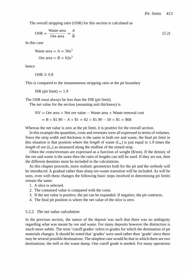
The overall stripping ratio (OSR) for this section is calculated as
OSR = Waste area
Ore area= A
B(5.2)
In this case
Waste area = A = 50u3
Ore area = B = 62u3
hence
OSR ∼= 0.8
This is compared to the instantaneous stripping ratio at the pit boundary
ISR (pit limit) = 1.9
The OSR must always be less than the ISR (pit limit).The net value for the section (assuming unit thickness) is
NV = Ore area × Net ore value − Waste area × Waste removal cost
= B × $1.90 − A × $1 = 62 × $1.90 − 50 × $1 = $68
Whereas the net value is zero at the pit limit, it is positive for the overall section.In this example the quantities, costs and revenues were all expressed in terms of volumes.
Since the strip width and thickness is the same in both ore and waste, the final pit limit inthis situation is that position where the length of waste (Lw) is just equal to 1.9 times thelength of ore (Lo) as measured along the midline of the mined strip.
Often the costs/revenues are expressed as a function of weight ($/ton). If the density ofthe ore and waste is the same then the ratio of lengths can still be used. If they are not, thenthe different densities must be included in the calculations.
As this chapter proceeds, more realistic geometries both for the pit and the orebody willbe introduced. A gradual rather than sharp ore-waste transition will be included. As will beseen, even with these changes the following basic steps involved in determining pit limitsremain the same:
1. A slice is selected.2. The contained value is compared with the costs.3. If the net value is positive, the pit can be expanded. If negative, the pit contracts.4. The final pit position is where the net value of the slice is zero.
5.2.2 The net value calculation
In the previous section, the nature of the deposit was such that there was no ambiguityregarding what was meant by ore and waste. For many deposits however the distinction ismuch more subtle. The term ‘cutoff grades’ refers to grades for which the destination of pitmaterials changes. It should be noted that ‘grades’ were used rather than ‘grade’ since theremay be several possible destinations. The simplest case would be that in which there are twodestinations: the mill or the waste dump. One cutoff grade is needed. For many operations
Pit limits 413

today there are three possible destinations: the mill, the leach dump and the waste dump.Each of the decisions
– mill or leach?– leach or waste?
requires a cutoff grade. A definition of cutoff grade which is often used (Davey, 1979):
Cutoff grade = the grade at which the mineral resource can no longer be processed ata profit.
applies to the simple ore-waste decision. This will be used in developing the preliminary pitlimits. The only destinations allowed are the waste dump or further processing. With thisdefinition the net value of material as a function of grade must be determined. That gradefor which the net value is zero is called the breakeven cutoff grade. This calculation will beillustrated using the example provided by Davey (1979) for copper. The copper ore is milledthereby producing a copper concentrate. This mill concentrate is shipped to a smelter andthe resulting blister copper is eventually refined.
In this example the following will be assumed:Mill recovery rate = 80%
Mill concentrate grade = 20%
Smelting loss = 10 lbs/st of concentrate
Refining loss = 5 lbs/st of blister copperThe steps of the net value computation are outlined below for an ore containing 0.55%copper. All of the costs and revenues will be calculated with respect to one ton of ore.
Step 1. Compute the amount of saleable copper (lbs/st of ore).
(a) Contained copper (CC) is
CC = 2000 lbs/st × 0.55
100= 11.0 lb
(b) Copper recovered by the mill (RM) is
RM = 11.0 × 80
100= 8.8 lb
(c) Concentration ratio (r). The ratio of concentration is defined as
r = lbs Cu/st of concentrate
lbs Cu recovered/st of ore(5.3)
Since the mill product runs 20% copper there are 400 lb of copper contained in one ton ofconcentrate. One ton of ore contains 8.8 lb of recoverable copper. Hence
r = 400
8.8= 45.45
This means that 45.45 tons of ore running 0.55% copper are required to produce 1 ton ofconcentrate running 20%.
(d) Copper recovered by the smelter (RS). The mill concentrate is sent to a smelter. Sincethe smelting loss is 10 lb/st of concentrate, the smelting loss (SL) per ton of ore is
SL = 10 lb/st of concentrate
45.45 tons of ore/st of concentrate= 0.22 lb
Open pit mine planning and design: Fundamentals414

Thus the recovered copper is
RS = 8.8 − 0.22 = 8.58 lb
(e) Copper recovered by the refinery (RR). The number of tons of ore required to produceone ton of blister copper is
2, 000 lb/st of blister copper
8.58 lb of copper/st of ore= 233.1
Since refining losses are 5 lb/st of blister copper, the refining loss (RL) per ton of ore is
RL = 5 lb of copper/st of blister copper
233 tons of ore/st of blister copper= 0.02 lb
Thus the recovered copper is
RR = 8.58 − 0.02 = 8.56 lb
Step 2. Compute the gross value (GV ) for the ore ($/st). The copper price assumed for thiscalculation is $1.00/lb. Furthermore there is a by-product credit for gold, molybdenum, etc.of $1.77/st of ore. Thus the gross value is
GV = 8.56 × $1 + $1.77 = $10.33
Step 3. Compute the associated total costs (TC) ($/st).
(a) Production (operating) costs (PC) excluding stripping are:
Mining $1.00Milling $2.80General and administration $0.57(15% of mining and milling)
PC = $4.37
(b) Amortization and depreciation (A&D). This amount is charged against each ton of oreto account for the capital investment in mine and mill plant. If the total A&D is $10,000,000and overall ore tonnage is 50,000,000 tons, then this value would be $0.20. In this particularcase, 20% of the total production costs will be used.
A&D = 0.20 × $4.37 = $0.87
(c) Treatment, refining and selling (TRS) cost.– Shipment of mill concentrate to the smelter. Since transport costs $1.40 per ton of
concentrate, the cost per ton of ore is
Concentrate transport = $1.40
45.45= $0.03
– Smelting cost. Smelting costs $50.00/st of concentrate. The smelting cost per tonof ore is
Smelting = $50.00
45.45= $1.10
Pit limits 415

– Shipment of the blister copper to the refinery. There is a transport cost of $50.00/st ofblister copper involved. The cost per ton of ore becomes
Blister transport = $50.008.58
2000= $0.21
– Refining cost. Refining costs $130.00/st of blister copper. The refining cost per ton ofore is
Refining = $130.008.58
2000= $0.56
– Selling and delivery cost (S&D). The selling and delivery cost is $0.01/lb of copper.Since 8.56 lb are available for sale
S&D = $0.09
– General plant (GP) cost. These costs amount to $0.07/lb of copper. Hence the GP costper ton of ore is
GP = $0.07 × 8.56 = $0.60
– Total treatment cost is
TRS = $2.59
(d) Total cost per ton of ore is
TC = $7.83
Step 4. Compute net value per ton of ore. The net value is the gross value minus the totalcosts. Thus for an initial copper content of 0.55%, the net value becomes
NV = GV − TC = $10.33 − $7.83 = $2.50
Step 5. Compute the net value for another ore grade. Steps 1 through 4 are now repeatedfor another copper content. In this case 0.35% Cu has been chosen. The by-product creditwill be assumed to vary directly with the copper grade. Hence
By-product credit = $1.770.35
0.55= $1.13
Assuming the recoveries and unit costs remain the same, the net value is −$0.30.
Step 6. Construct a net value – grade curve. The two points on a net value – grade curvewhich have been determined by the process outlined above
Point Net value ($/st) Grade (% Cu)1 $2.50 0.552 −$0.30 0.35
are plotted in Figure 5.6. Assuming that the net value – % Cu relationship is linear it ispossible to find an equation of the form y = a + bx relating net value (y) to grade (x). Theresult is
y = −$5.20 + $14.0x
where y is the net value ($/st of ore) and x is the percent copper.
Open pit mine planning and design: Fundamentals416

Net
Val
ue (
$/to
n)$3.00
$2.00
$1.00
$–1.00
0.2
(0.35, –0.30)
� �$5.20 � 14.0 x
0.4 0.6 0.8 1.00
Ore Grade (% Cu)
Y
(0.55, 2.50)
Figure 5.6. Net value – ore grade curve.
Step 7. Determine the breakeven cutoff grade (for application at the pit limit). The breakevencutoff grade is defined as that grade for which the net value is zero. One can determine thatpoint by inspecting Figure 5.6 or by solving the equation found in Step 6 for y = 0. Onefinds that
x (breakeven) = 0.37% Cu
Step 8. Developing a stripping ratio – grade curve. The cutoff grade distinguishes thatmaterial which can be mined and processed with a net value greater than or equal to zero.Material with a zero net value cannot pay for any stripping. Thus it must be exposed atthe surface or be overlying richer blocks which can pay for the required stripping. Assumethat the cost for stripping 1 ton of waste is $1.00. Ore with a net value of $1.00 can pay forthe stripping of 1 ton of waste. Ore with a net value of $2.00/ton can pay for the strippingof 2 tons of waste, etc. The stripping ratio axis has been added in Figure 5.7 to show this.The net value – grade equation
NV = −$5.20 + $14.00 × (% Cu) (5.4)
can be modified to yield the stripping ratio (SR) – grade relationship
SR = −$5.20 + $14.00 × (% Cu) (5.5)
For a grade of 0.55% Cu, the breakeven stripping ratio is
SR (0.55%) = 2.5
Pit limits 417

Net
Val
ue (
$/to
n)$3.00
$2.00
$1.00
$�1.00
0.2 0.4 0.6 0.8 1.000
1:1
2:1
3:1
Bre
akev
en S
trip
ping
Rat
io
Ore Grade (% Cu)
Figure 5.7. Net value and breakeven stripping ratio versus ore grade.
$3.00
$2.00
$1.00
$–1.00
00.2 0.4 0.6 0.8 1.0
Ore Grade (% Cu)
(0.3,–1.00)
3:1
2:1
1:1
Bre
akev
en S
trip
ping
Rat
io
Net
Val
ue (
$/to
n)
Figure 5.8. Addition of the minimum value portion.
This was as expected since the net value is $2.50 and the stripping cost is $1.00
SR = $2.50
$1.00= 2.50
Step 9. Presenting the final curves. The net value – grade curve should be completedby the addition of the cost of stripping line (SC). This is shown in Figure 5.8. It shouldbe noted that no material can ever have a value less than that of waste. In this case
Open pit mine planning and design: Fundamentals418

7:1
6:1
5:1
3:1
2:1
1:1
0.3 0.4 0.5 0.6 0.7 0.8 0.9
4:1
Ore Grade (% Cu)
Str
ippi
ng R
atio
Figure 5.9. Stripping ratio – ore grade curveused for pit limit determinations (Koskiniemi,1979).
the value of waste is −$1.00. The horizontal line (NV = −$1.00) and the NV-grade line(NV = −5.20 + 14.00 × (% Cu)) intersect at a grade of
% Cu = 0.30
For grades less than 0.30%, the material is considered as waste with respect to milling.Depending upon the economics, some other treatment process such as dump leaching maybe possible. When using hand methods all material having grades less than the breakevencutoff (0.37% in this case) is considered as waste. The final stripping ratio-grade curve isshown in Figure 5.9.
For the computer techniques discussed later, the portion of the curve lying between 0.30and 0.37% Cu is also included.
5.2.3 Location of pit limits – pit bottom in waste
The application of this curve to locating the final pit wall positions will be illustrated usingthe vertical section (Fig. 5.10) taken through the block model. The basic process used hasbeen presented by Koskiniemi (1979). Locating the pit limit on each vertical section is a trialand error process. It will be assumed that
– Pit slopes:Left hand side = 50◦;Right hand side = 40◦;
– Minimum width of the pit bottom = 100 ft;– Material densities:
Ore = 165 lb/ft3;Waste rock = 165 lb/ft3;Overburden = 165 lb/ft3;
Pit limits 419

Figure 5.10. Pit limit determination with bottom in waste (Koskiniemi, 1979).
Table 5.1. Bottom in waste: pit limit guess #1 (Line G1).
Length (ft) Ore grade Ore length ×(goi) ore grade (loigoi)
Overburden (lob) Waste (lw) Ore (loi)
130296
30 0.6 18.052 0.7 36.452 1.0 52.052 0.9 46.852 0.8 41.6
130 296 238 g = 0.82 194.8
SR (actual) = 130+296238
∼= 1.79 : 1;SR (allowable) ∼= 6.2 : 1;Conclusion: move to the left.
– Relative mining characteristics:Waste rock = 1;Overburden = 1;
– The stripping ratio – ore grade curve of Figure 5.9 applies;– The pit bottom is at the ore-waste contact.
Overburden as defined here means soil, glacial till, gravel, highly weathered rock, etc.not requiring drilling and blasting prior to removal. Waste rock, on the other hand, doesrequire drilling and blasting. The general procedure will be demonstrated with respect tothe left-hand slope.
Step 1. A trial slope (guess #1) is drawn through the section. The lengths and grades areentered into a table such as Table 5.1. The purpose will be to obtain the average ore gradeand stripping ratio along this line. The lengths can simply be scaled off the section withenough accuracy. The cutoff grade is 0.37% Cu.
Open pit mine planning and design: Fundamentals420

Table 5.2. Bottom in waste: pit limit guess #2 (Line G2).
Length (ft) Ore grade Ore length ×(goi) ore grade (loigoi)
Overburden (lob) Waste (lw) Ore (loi)
130385
52 0.8 41.652 0.7 36.452 0.8 41.6
130 385 156 g = 0.77 119.6
SR (actual) = 130 + 385156
∼= 33 : 1;SR (allowable) ∼= 5.6 : 1;Conclusion: move to the left.
Table 5.3. Bottom in waste: pit limit guess #3 (Line G3).
Length (ft) Ore grade Ore length ×(goi) ore grade (loigoi)
Overburden (lob) Waste (lw) Ore (loi)
130443
52 0.5 26.052 0.8 41.6
130 443 104 g = 0.65 67.6
SR (actual) = 130 + 443104
∼= 5.51 : 1;SR (allowable) ∼= 3.9 : 1;Conclusion: move to the right.
Table 5.4. Bottom in waste: pit limit guess #4 (Line G4).
Length (ft) Ore grade Ore length ×(goi) ore grade (loigoi)
Overburden (lob) Waste (lw) Ore (loi)
130435
52 0.7 36.452 0.8 41.6
130 435 104 g = 0.75 78.0
SR (actual) = 130 + 435104
∼= 5.43 : 1;SR (allowable) ∼= 5.4 : 1;Conclusion: final limit.
Step 2. The average ore grade is determined. The products of ore grade × ore length aredetermined (loigoi) and summed (
∑(loigoi)). The sum of the ore lengths is found (
∑loi).
The average ore grade g is found from
g =∑
loigoi∑loi
= 0.82% Cu (5.6)
Pit limits 421

Figure 5.11. Allowable stripping ratiofor a grade of 0.82%.
Step 3. The stripping ratio for this line is determined. This must be expressed in the sameform as the stripping ratio – ore grade curve. In this case it is required to have tons of wasteper ton of ore. Since the densities are all equal and the relative diggability of the overburdenand the waste rock is the same, the stripping ratio is simply the ratio of the lengths.
SR = Length overburden + Length waste rock
Length ore= lob + lw
lo
SR = 130 + 296
238∼= 1.79 (5.7)
Step 4. Determination of the allowable stripping ratio for average ore grade using the SR –ore grade curve (Fig. 5.11). In this case one finds that
SR (allowable) ∼= 6.2 : 1
Step 5. Comparison of the actual and allowable SR. Since the actual stripping ratio
SR (actual) = 1.79 : 1
is much less than that allowable (6.2 : 1), the pit slope can be moved to the left.
Step 6. A new guess of the final pit slope location is made and the process repeated. Thisiteration process is continued until the actual and allowable stripping ratios are close.
Conclusion: Guess #4 is the final position of the left hand slope. Note that the blockhaving grade 0.3 is considered waste since it is below cutoff.
Step 7. Determination of right-hand slope position. The same process is repeated for theright hand wall of the pit. The results are shown in Figure 5.10. The final pit bottom hasa width of about 215 ft.
Open pit mine planning and design: Fundamentals422

Table 5.5. Bottom in ore: pit limit guess #1 (Line G1).
(a) Left hand side
Length (ft) Ore grade Ore length ×(goi) ore grade (loigoi)
Overburden (lob) Waste (lw) Ore (loi)
130330
48 0.7 33.652 0.8 41.613 0.7 9.139 0.9 35.122 0.8 17.650 0.8 40.0
130 330 224 g = 0.79 177.0
SR (actual) = 130 + 330224
∼= 2.05;SR (allowable) ∼= 6 : 1.
(b) Right hand side
Length (ft) Ore grade Ore length ×(goi) ore grade (loigoi)
Overburden (lob) Waste (lw) Ore (loi)
143283
48 0.6 28.813
48 1.0 48.070 0.9 63.011 0.8 8.857 0.9 51.326 1.0 26.039 1.0 39.011 0.8 8.8
143 296 310 g = 0.88 273.7
SR (actual) = 143 + 296310
∼= 1.42 : 1;SR (allowable) ∼= 7 : 1;Conclusion: the pit can be ‘floated’ considerable deeper.
If the waste/overburden have densities different from the ore, then the calculation ofstripping ratio using simple length ratios does not work. The generalized stripping ratiocalculation becomes
SR = lobρob + lwρw
loρo(5.8)
where ρob is the overburden density, ρw is the waste density, and ρo is the ore density. Ifthe mineability characteristics of the overburden and waste rock are different, then the costsinvolved in their removal will also be different. It will be recalled that a single waste mining
Pit limits 423

Table 5.6. Bottom in ore: pit limit guess #2 (Line G2).
(a) Left hand side
Length (ft) Ore grade Ore length ×(goi) ore grade (loigoi)
Overburden (lob) Waste (lw) Ore (loi)
139626
52 0.5 26.052 0.6 31.252 0.6 31.252 0.6 31.252 0.6 31.252 0.6 31.2
139 626 258 g = 0.58 150.8
SR (actual) = 139 + 626258
∼= 2.97 : 1;SR (allowable) ∼= 2.95 : 1.
(b) Right hand side
Length (ft) Ore grade Ore length ×(goi) ore grade (loigoi)
Overburden (lob) Waste (lw) Ore (loi)
157617
65 0.6 39.061 0.6 36.665 0.5 32.561 0.5 30.550 0.6 30.0
157 617 302 g = 0.56 168.6
SR (actual) = 157 + 617302
∼= 2.56 : 1;SR (allowable) ∼= 2.6 : 1;Conclusion: guess #2 is close to the pit slope location.
cost was used in the development of the SR – grade curves. Assume that the given cost(Cw/ton) applies to waste rock and that the overburden removal cost is αCw/ton. The factorα is the relative mining cost of the overburden to that of the waste rock. The stripping ratioformula can be further modified to
SR = αlobρob + lwρw
loρo(5.9)
If the cost/ton to remove the overburden is only half that of the waste rock then α = 0.5. Thisfactor changes the overburden into an equivalent waste rock. If the cost used to develop theSR – grade curve had been based on overburden, then one needs to convert waste rock intoequivalent overburden.
Open pit mine planning and design: Fundamentals424

Figure 5.12. Final pit limits with bottom in ore.
5.2.4 Location of pit limits – pit bottom in ore
Figure 5.12 shows the case when the orebody continues to depth. Assume as before that
Left hand slope = 50◦
Right hand slope = 40◦
Minimum pit bottom width = 100 ft
Since the pit bottom is now in ore, the costs for stripping can be paid for by the ore in thestrip along the pit bottom as well as that along the pit sides. A 50 ft wide allocation is madeto both the right and left hand sides. The procedure is similar to that described with the pitbottom in waste. However, now both sides and the bottom must be examined at the sametime. The procedure is as follows:
Step 1. Draw to scale a final pit profile using the appropriate left and right hand slopes aswell as the minimum pit bottom on a piece of tracing paper. Superimpose this on the section.Guess an initial position.
Step 2. Calculate the average ore grades and stripping ratios for the left and right hand sides.Compare these to the allowable values. For simplicity it will be assumed that the densitiesand mineabilities of the materials involved are the same.
Because of the freedom of the pit to ‘float’ both vertically and horizontally, the iterativeprocedure can be quite time consuming.
5.2.5 Location of pit limits – one side plus pit bottom in ore
A third possible situation is one in which one of the pit slopes is in ore. In Figure 5.13 itwill be assumed that the right hand slope follows the ore-waste contact, the left hand slopeis at 50◦, and a minimum pit bottom width is 100 ft. In this case the ore along the pit bottom
Pit limits 425

Figure 5.13. Final pit limits with right hand side in ore.
Table 5.7. Final pit limit location for one side plus pit bottom in ore (Fig. 5.13).
Length (ft) Ore grade Ore length ×(goi) ore grade (loigoi)
Overburden (lob) Waste (lw) Ore (loi)
130626
43 0.5 12.552 0.4 20.852 0.6 31.252 0.6 31.252 0.4 20.8
100 0.6 60.0
130 626 351 g = 0.53 185.5
SR (actual) = 130 + 626351
∼= 2.15;SR (allowable) ∼= 2.21;Conclusion: this is the final pit location.
contributes to the cost of stripping the left wall. The approximate position of the final pit isshown superimposed on the figure. The corresponding calculation is given in Table 5.7.
5.2.6 Radial sections
The types of sections used depends upon the shape of the orebody. For the elongated orebodyshown in Figure 5.14, transverse sections yield the best representation in the central portion.Along the axis of the orebody, a longitudinal section may be taken.
Transverse sections such as 1-1′, 2-2′, etc. in Figure 5.14 have been constructed parallelto one another and normal to the orebody axis. The influence of these sections is assumed toextend halfway to the neighboring sections. They are of constant thickness by construction
Open pit mine planning and design: Fundamentals426

Figure 5.14. Plan view of orebody illustrating the different section types (Koskiniemi, 1979).
Figure 5.15. Isometric view of a parallel section.
(Fig. 5.15). A small face area (�A) at location A at the crest of the pit represents the samevolume as the same area located at the toe (location B).
The pit location procedures described in Subsections 5.2.3 through 5.2.5 apply with-out modification to parallel cross-sections and longitudinal sections. As can be seen inFigure 5.14, radial sections are often needed to describe pit ends. For radial sections such
Pit limits 427

Figure 5.16. Isometric view of a radialsection.
Figure 5.17. Plan representationshowing the area of influence for aradial section (Koskiniemi, 1979).
as shown in Figure 5.16, the volume represented by an area �A at the crest (location C) ismuch greater than one at D due to the varying section thickness.
A modification in the procedure used to locate the final pit limit is required. This isaccomplished through the development of a curve relating the apparent stripping ratio asmeasured on the radial section to the true stripping ratio.
Figure 5.17 is a plan view showing the region at the end of the pit in which radial sectionsare being used.
Open pit mine planning and design: Fundamentals428

Figure 5.18. Isometric view of theradial sector.
a. Radial Section
a
b
Waste
a/cos u b/cos u
Ore
u
b. Plan Section
a/cos u b/cos uRadialSection
b
B �A�
Figure 5.19. Plan and section views of the radialsector shown in Figure 5.18.
Figure 5.18 is an isometric view of the sector in question. The exposed ore area is identifiedas A and that of waste as B. The apparent (measured) stripping ratio for the radial sectionas shown on Figure 5.19a would be
SR (measured) = b
a(5.10)
Pit limits 429

Figure 5.20. The ore and waste areas involved.
From the plan projection of the wall surface for this sector as shown in Figure 5.19b, thearea of ore is A′ and that of waste B′. Since the included angle for the sector is β, the oreradius in this projection is a/ cos β and the thickness of the waste zone is b/ cos θ.
The calculation of the plan projected areas is shown in Figure 5.20. The true strippingratio can be expressed as
SR (true) = B′
A′ = (a + b)2 − a2
a2=
(1 + b
a
)2
− 1
Since the measured stripping ratio on the section is as shown in Equation (5.10) then
SR (true) = (1 + SR (measured))2 − 1 (5.11)
As can be seen, this relationship is independent of both the slope angle and the includedangle.
Values of SR (true) and SR (measured) are presented in Table 5.8 and plotted in Figure5.21. The steps in the location of the final pit limit on a radial section are outlined below:
Step 1. As with parallel sections, one guesses the location of the final pit slope and calculatesthe average ore grade g and the stripping ratio. Assume that g = 0.8 and the measuredstripping ratio is 2 : 1.
Open pit mine planning and design: Fundamentals430

Table 5.8. Comparison of true versus measured strippingratios for radial sections.
Stripping ratio
Measured True
0 00.25 0.560.50 1.250.75 2.061.0 3.01.25 4.061.5 5.252.0 8.02.5 11.253.0 15.0
16
14
12
10
8
6
4
2
True
SR
1 2 3 4Measured SR
Figure 5.21. True versus measured strip-ping ratios (Koskiniemi, 1979).
Step 2. With parallel sections one would go directly to the SR – %Cu curve to see whatstripping ratio this grade would support. In the case shown in Figure 5.22, it is about 6 : 1indicating that the limit could be moved outward. For radial sections one must proceed toStep 3.
Step 3. The measured stripping ratio must first be converted to a true stripping ratio throughthe use of the conversion curve (Fig. 5.21). This indicates that for a measured stripping ratioof 2 : 1, the true stripping ratio is 8 : 1.
Step 4. Returning to Figure 5.22, one finds that the grade required to support a strippingratio of 8 : 1 is 0.94. This is higher than the 0.8 present and hence the next guess of the finalpit limit should be moved toward the pit.
Pit limits 431

9:1
8:1
7:1
6:1
5:1
4:1
3:1
2:1
1:1
00.3 0.4 0.5 0.6 0.7 0.8 0.9 1.0
Ore Grade (% Cu)
Str
ippi
ng R
atio
Figure 5.22. Example of stripping ratio calculation for a radial section.
In summary, the treatment of radial sections is done in exactly the same way as withparallel sections except that the use of an intermediate curve to convert measured SR totrue SR is required. It should be pointed out that the ore region is pie-shaped and strictlyspeaking a weighted average approach should be used to calculate an average ore grade.
5.2.7 Generating a final pit outline
Once final pit profiles have been located on the individual sections, they must be evaluatedas a group to examine how they fit together relative to one another. One section may suggesta very narrow pit, for example, whereas the adjacent ones yield a wide one (see Fig. 5.23).This smoothing requires adjustments to be made to the various sections. The easiest wayof visualizing the pit and performing this task is through the use of level plans (horizontalsections). The final ore reserve estimation will also be done using plans. Thus to proceedrequires the development of a composite mine plan map from the vertical sections.
The steps are outlined below (Koskiniemi, 1979):
Step 1. Transfer of intercepts to plan map. The locations of the pit bottom and the surfaceintercepts of the pit limits are transferred from the vertical sections to the plan map.
Step 2. Handling of discontinuous slopes. If a vertical section does not have a continuousslope line from the pit bottom to the surface intercept this is also shown.
Open pit mine planning and design: Fundamentals432pj
wst
k|40
2064
|143
5603
464

Figure 5.23. A series of initial pit outline sectionsfor an orebody.
Step 3. Deciding on initial bench design location. The actual design of the composite plangenerally begins with the pit bottom working upward. (Some designers prefer however tobegin the design with a middle bench and work both upwards and downwards.)
Step 4. Smoothing. The points from the sections usually present a very irregular pattern,both vertically and horizontally. In smoothing these and designing the bottom bench severalthings should be kept in mind (Koskiniemi, 1979):
– Averaging the break-even stripping ratios for adjoining sections. If one section is movedsignificantly inward or outward, major changes in stripping/ore reserves may result. Thusthe sections are carefully evaluated with each change.
– Use of simple geometric patterns for ease of design. The simpler the geometric shape,the easier it is to design the remainder of the pit.
– Location of ramp to pit bottom.– Watching for patterns that might lead to slope stability problems. For example bulges
or noses in the pit often are sources of problems.
Pit limits 433

Figure 5.24. Plan view of a pit with constant slope angle.
Figure 5.25. Plan view of a pit containing a wide bench.
Step 5. The bottom bench is then drawn. As has been discussed in Chapter 4, there areseveral possibilities for depicting the geometry. One way is to show both the toe and crestlines. Depending upon map scale and the number of benches, this may or may not be good.A second possibility is to display just one (either the toe or the crest) since the position ofthe other can be easily obtained knowing the bench height and the bench face angle.
The third possibility is to show the median elevation line (half the distance up the benchface). This is the representation most commonly used and that employed here.
Step 6. Addition of the median lines for the overlying benches. In preliminary designs theroads are often not shown. In such cases, the plan distance between the median lines is:
Md = H
tan θ(5.12)
where Md is the plan distance between median lines, H is the bench height and θ is theoverall pit slope angle. An overall pit slope angle is chosen so that the space required for theroad is included. For the case shown in Figure 5.24, the slope angle is the same throughoutthe pit and the slope is continuous from toe to crest and hence the median lines are paralleland equally spaced. Figure 5.25 shows the case when there is a wide bench part way upthe pit. Figure 5.26 shows the case when the north and south side slope angles are different.
Open pit mine planning and design: Fundamentals434

Figure 5.26. Plan view of a pit with different north and south wall slopes.
Figure 5.27. Composite ultimate pit plan (Koskiniemi, 1979).
If in the final designs the actual roads are shown, then the horizontal distance Md betweenthe median lines is equal to
Md = bw + H
tan θf(5.13)
where bw is the level berm width, H is the bench height, and θf is the bench face angle. Acomposite ultimate pit plan with a road included is shown in Figure 5.27. The procedurethrough which a road is added to a pit has been discussed in Chapter 4.
Step 7. Transfer of the pit limits to the individual level plans. When the composite pitplan has been completed, the pit limits are transferred to the individual level plans (Fig.5.28). Through this process, the design engineer will first check the stripping ratios at thefinal pit limit. The pit is split into sectors such as shown in Figure 5.29, and the ore-wasterelationships checked.
Pit limits 435

Figure 5.28. Level plan of bencha with the ultimate pit limit super-imposed (Koskiniemi, 1979).
Figure 5.29. Plan of the ultimate pit showing the sectors (Soderberg & Rausch, 1968).
Figure 5.30 shows the median lines and ore grades for a sector taken in the center of thepit. If the pit bottom is in ore then this effect is included simply by adding artificial medianlines to this region.
In this case the average grade is 0.7 and the stripping ratio is
SR = 3
4= 0.75
A radial section is shown in Figure 5.31. In this case
g =∑
rigi∑ri
= 0.9 × 1 + 0.8 × 2 + 0.6 × 3 + 0.5 × 4
1 + 2 + 3 + 4= 0.63
Open pit mine planning and design: Fundamentals436

Figure 5.30. Average grade calculationfor a parallel sector.
Figure 5.31. Average grade calculation fora radial sector.
The stripping ratio is
SR =∑
rwi∑roi
= 5 + 6 + 7
1 + 2 + 3 + 4= 1.8
The general procedure is to measure and sum the lengths of waste and ore on each level atthe pit limit within a given sector. The ratio gives the stripping ratio. The average grade is thelength weighted average. The grade and stripping ratio values for each sector are comparedto the SR – grade curve. Anomalous areas are identified and the design reviewed to see whatcorrections can be made.
Step 8. Calculation of ore reserves by level. The calculation of final ore reserves and overallstripping ratio is done using the level maps. For each level the ore tons and grade andthe waste tons are determined within the ultimate pit limits. Assuming that the block sizein Figure 5.28 is 100′ × 100′ × 40′ and that the tonnage factor is 12.5 ft3/ton, then eachwhole block contains 32,000 tons. A tabulation of the reserves on this level is presented inTable 5.9. Ore is considered to be that material within the pit limits having a grade equalto or greater than the grade from the stripping curve at a break-even stripping ratio of zero.This is generally called the ore reserve cut off grade. Using a cutoff grade of 0.37%, thetotal tons of ore and waste are computed. The average ore grade is also obtained.
Step 9. Calculation of final ore reserve and overall stripping ratio. The ore reserves for eachlevel are tabulated such as shown in Table 5.10. From this the ore tons, overall average oregrade, total waste tons and overall stripping ratio can be found. In addition tonnage-gradedistribution curves are often plotted both overall and by level to help in mill design andsetting of production levels.
5.2.8 Destinations for in-pit materials
Once the pit limits have been defined, all of the material within the pit outline will be minedirrespective of its value. Given mined material the decision must be made regarding its
Pit limits 437

Table 5.9. Reserve summary for bench A.
Grade (%) Tons ore Tons waste
<0.30 125,3000.30–0.36 00.37–0.39 00.40–0.49 00.50–0.59 193,3400.60–0.69 192,0000.70–0.79 144,4000.80–0.89 189,0000.90–0.99 32,0001.00–1.09 32,000
Table 5.10. Total reserves within the final pit outline.
Bench Grade
<0.30 0.3–0.36 0.37–0.39 0.4–0.49 0.5–0.59 0.6–0.69 0.7–0.79 0.8–0.89 0.9–0.99 1.0–1.09
A 125,300 0 0 0 193,340 192,000 144,400 189,000 32,000 32,000BCDEFGHIJTotals
destination. A new cutoff grade based simply upon meeting the processing costs can becalculated. For the example presented in Section 5.2.2, the direct mining cost was givenas $1 per ton. If this is subtracted from the total cost then the net value – grade equationbecomes
y = −4.2 + 14.0 x
Solving for the breakeven cutoff grade (sending to the mill or the dump) one finds that
x = 0.30% Cu
Hence for the pit material everything having a grade greater than or equal to 0.30% Cu couldbe sent to the mill. This assumes, of course, that the transport costs to the dumps and themill are the same. If not, then the cost differences can be included. Such considerations canbe made only if mill capacity is available. Often this is not the case. The economics of thismarginal/submarginal material must be evaluated very closely.
Open pit mine planning and design: Fundamentals438
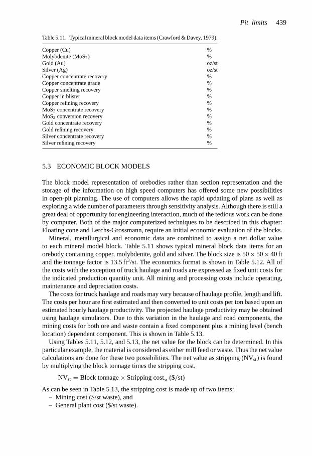
Table 5.11. Typical mineral block model data items (Crawford & Davey, 1979).
Copper (Cu) %Molybdenite (MoS2) %Gold (Au) oz/stSilver (Ag) oz/stCopper concentrate recovery %Copper concentrate grade %Copper smelting recovery %Copper in blister %Copper refining recovery %MoS2 concentrate recovery %MoS2 conversion recovery %Gold concentrate recovery %Gold refining recovery %Silver concentrate recovery %Silver refining recovery %
5.3 ECONOMIC BLOCK MODELS
The block model representation of orebodies rather than section representation and thestorage of the information on high speed computers has offered some new possibilitiesin open-pit planning. The use of computers allows the rapid updating of plans as well asexploring a wide number of parameters through sensitivity analysis. Although there is still agreat deal of opportunity for engineering interaction, much of the tedious work can be doneby computer. Both of the major computerized techniques to be described in this chapter:Floating cone and Lerchs-Grossmann, require an initial economic evaluation of the blocks.
Mineral, metallurgical and economic data are combined to assign a net dollar valueto each mineral model block. Table 5.11 shows typical mineral block data items for anorebody containing copper, molybdenite, gold and silver. The block size is 50 × 50 × 40 ftand the tonnage factor is 13.5 ft3/st. The economics format is shown in Table 5.12. All ofthe costs with the exception of truck haulage and roads are expressed as fixed unit costs forthe indicated production quantity unit. All mining and processing costs include operating,maintenance and depreciation costs.
The costs for truck haulage and roads may vary because of haulage profile, length and lift.The costs per hour are first estimated and then converted to unit costs per ton based upon anestimated hourly haulage productivity. The projected haulage productivity may be obtainedusing haulage simulators. Due to this variation in the haulage and road components, themining costs for both ore and waste contain a fixed component plus a mining level (benchlocation) dependent component. This is shown in Table 5.13.
Using Tables 5.11, 5.12, and 5.13, the net value for the block can be determined. In thisparticular example, the material is considered as either mill feed or waste. Thus the net valuecalculations are done for these two possibilities. The net value as stripping (NVst) is foundby multiplying the block tonnage times the stripping cost.
NVst = Block tonnage × Stripping costst ($/st)
As can be seen in Table 5.13, the stripping cost is made up of two items:– Mining cost ($/st waste), and– General plant cost ($/st waste).
Pit limits 439

Table 5.12. Block model mining and processing cost items (Crawford & Davey, 1979).
Drilling $/st ore and wasteBlasting $/st ore and wasteLoading $/st ore and wasteHauling $/truck hourHaul roads $/truck hourWaste dumps $/st wastePit pumping $/st oreMine general $/st ore
$/st wasteOre reloading $/st oreOre haulage $/st oreConcentrating $/st oreConcentrate delivery $/st concentrateSmelting $/st concentrateGeneral plant $/st ore
$/st waste$/st blister
Blister casting loading and freight $/st blisterRefining $/st blisterSelling and delivery $/lb refined copper
Metal pricesCopper $/lbMoS2 $/lbGold $/ozSilver $/oz
Table 5.13. Pit limit analysis cost summary (Crawford & Davey, 1979).
Stripping (waste) Mill feed (ore)
Mining ($/st) aL∗ + b cL∗ + dProcessing and other:
Ore haulage ($/st ore) XConcentrating ($/st ore.) XConcentrate delivery ($/st conc.) XSmelting ($/st conc.) XBlister casting loading, and freight X
($/st blister)General plant
$/st ore X$/st waste X X$/st blister X
Refining ($/st blister) XSelling and delivery($/lb Cu) X
* Level elevation.
With regard to the second cost item (general plant), there are many ‘overhead’ types of costswhich are independent of whether the material being moved is ‘ore’ or ‘waste’.
Although, in the end, the ‘ore’ must pay for all of the costs, there is some logic forallocating general plant costs to the waste as well (see Subsection 2.4.1).
Open pit mine planning and design: Fundamentals440

Table 5.14. Block evaluation calculation format.
Block dataBlock location Data for blockBlock tonnage from Table 5.11 and 5.13
As mill feed*Revenue from metal sales ($)Copper: Block tonnage × lb saleable Cu/st × Price ($/lb) = AMoS2 = BGold = CSilver = D
Total revenue RCost of copper ($):
Block tonnage × lb saleable Cu/st × Cost ($/lb) = C′Net value as mill feed ($):
NVmf ($) = R − C′Net value as stripping ($):
NVst($) = Block tonnage × Stripping cost ($/st)
* The block is designated as mill feed and assigned NVmf if net value is greater than NVst, even if negative.
The net value as mill feed (NVmf) requires the calculation of the revenues and costs(excluding any stripping) for the block. Table 5.14 summarizes the calculations. The millfeed and stripping net values are compared for each block and the most positive value isassigned. This net value then becomes the only piece of block data used directly in themining simulators.
5.4 THE FLOATING CONE TECHNIQUE
In the section on manual techniques for determining the final pit limits, it was shown that fora single pit wall, the line having the slope angle defining the wall was moved back and forthuntil the actual grade and stripping ratio matched a point on the SR-grade curve. For thecase when both walls and the pit bottom were in ore, a geometric figure in the shape of theminimum pit was constructed and moved around on the section (vertically and horizontally)until the stripping ratios and grades measured along the periphery matched that from thecurve. For the case of 45◦ slopes and a 100 ft minimum pit bottom width, the figure to be‘floated’ is as shown in Figure 5.32. If this figure is revolved around the axis, the solidgenerated is called the frustum of a cone. Had the minimum pit width been zero, then thefigure would simply be a cone. With sections it was most convenient to use two-dimensionalrepresentation and not consider the effect of adjacent sections. This was at least partiallydone later through the smoothing on plan.
Although there are other techniques for determining the final pit configuration, currentlythe most popular is through the use of this ‘floating cone’. Several changes in the manualprocess are necessary to accommodate the computer. In the manual process, a net value –grade curve was developed. Knowing the cost of waste removal, this curve was changed intoa SR – grade curve. The user then simply evaluated stripping ratio (normally by measuringlengths of ore and waste) and calculated the weighted average grade. Through the use ofthe SR-grade ‘nomograph’ one could examine pit expansion.
Pit limits 441

Figure 5.32. Pit profile to be ‘floated’.
Net
Val
ue (
$/to
n)
5
4
3
2
1
0
�1
�2
0.2 0.4 0.6 0.8 1.0 1.2 1.4 1.6 1.8
Grade (% Cu)
Waste Mill Feed
SR
2:1
1:1
Figure 5.33. Net value – grade curve showing the waste/mill feed split.
When using the computer, it is more convenient to use the net values of the blocks directly.Figure 5.33 shows the type of net value-grade curve which is actually used. Consider thesimple example shown in Figure 5.34. This case will be examined using both the manualmethod based upon grades and stripping ratios, and that in which net values are assigned tothe blocks. Three potential pit limits have been superimposed on the grade block model ofFigure 5.35. A pit slope of 45◦ is assumed. The average ore grades and stripping ratios aregiven. The final pit is represented by case 3.
Using Figure 5.33, the grade block model of Figure 5.34 can be converted into an economicblock model. The result is shown in Figure 5.36. By examining the net values of the blocksinvolved in a particular mining sequence, final pit limits can be determined. Mining isstopped when the net value is negative. The net values for the three cases examined inFigure 5.35 are given in Figure 5.37.
Slice 3 has a NV = 0 and would define the final pit on this section. As can be seen themanual and economic block approaches give equivalent results. The net value approach isby far the easiest to program, particularly when considering a three dimensional array ofblocks.
Open pit mine planning and design: Fundamentals442

Figure 5.34. Grade block modelfor pit limit example.
Figure 5.35. Trial final pit lim-its based on the manual proce-dure. Case 3 is the final limit.
Figure 5.36. Correspondingeconomic block model.
Figure 5.37. Trial final pit limits.
Pit limits 443

Figure 5.38. Block model for Example 1 (Barnes,1982).
Figure 5.39. Stepped cone pit model.
The principles involved in determining the pit outline, given an entire 2-dimensional arrayof blocks will now be demonstrated. The examples were originally presented by Barnes,1982. Figure 5.38 shows the sample section to be considered with the net values given. Theblocks are equidimensional and the slope angle will be 45◦. This means that slope is formedby going up one and over one block. Figure 5.39 shows the stepped cone which will be usedfor determining the final pit.
The following steps are used:
Step 1. The cone is ‘floated’ from left to right along the top row of blocks in the section. Ifthere is a positive block it is removed.
Step 2. After traversing the first row, the apex of the cone is moved to the second row.Starting from the left hand side it ‘floats’ from left to right stopping when it encounters thefirst positive block. If the sum of all the blocks falling within the cone is positive (or zero),these blocks are removed (mined). If the sum is negative the blocks are left, and the conefloats to the next positive block on this row. The summing and mining or leaving process isrepeated.
Step 3. This floating cone process moving from left to right and top to bottom of the sectioncontinues until no more blocks can be removed.
Step 4. The profitability for this section is found by summing the values of the blocksremoved.
Step 5. The overall stripping ratio can be determined from the numbers of positive (+) andnegative (−) blocks.
These rules can now be applied to the section shown in Figure 5.38. There are four positiveblocks in the model hence there are four corresponding cones which must be evaluated. Usinga top–down rule, the block at row 1/column 6 would initiate the search. Since there are nooverlying blocks, the value of the cone is the value of the block: 1. The value is positive, sothe block is mined (Fig. 5.40).
Open pit mine planning and design: Fundamentals444pj
wst
k|40
2064
|143
5603
473
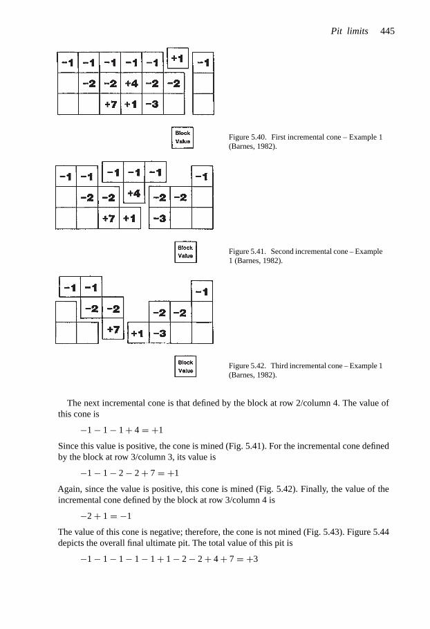
Figure 5.40. First incremental cone – Example 1(Barnes, 1982).
Figure 5.41. Second incremental cone – Example1 (Barnes, 1982).
Figure 5.42. Third incremental cone – Example 1(Barnes, 1982).
The next incremental cone is that defined by the block at row 2/column 4. The value ofthis cone is
−1 − 1 − 1 + 4 = +1
Since this value is positive, the cone is mined (Fig. 5.41). For the incremental cone definedby the block at row 3/column 3, its value is
−1 − 1 − 2 − 2 + 7 = +1
Again, since the value is positive, this cone is mined (Fig. 5.42). Finally, the value of theincremental cone defined by the block at row 3/column 4 is
−2 + 1 = −1
The value of this cone is negative; therefore, the cone is not mined (Fig. 5.43). Figure 5.44depicts the overall final ultimate pit. The total value of this pit is
−1 − 1 − 1 − 1 − 1 + 1 − 2 − 2 + 4 + 7 = +3
Pit limits 445

Figure 5.43. Fourth incremental cone – Example 1(Barnes, 1982).
Figure 5.44. Ultimate pit – Example 2 (Barnes,1982).
The overall stripping ratio is
SR (overall) = 7
3In this simple situation, the final pit is ‘optimal’. Over the years, considerable effort hasbeen spent in trying to develop procedures which when applied would yield the ‘optimal’pit. The ‘optimum’ might be defined for example, as the one yielding one of the following,
– maximum profit,– maximum net present value,– maximum extraction.
Although many contend that the determination of such an ‘optimum’ pit is largely of aca-demic interest due to changing prices, costs and poorly defined grades, none-the-less effortscontinue in this direction. Barnes (1982) has presented three problems representing floatingcone situations not leading to an optimum pit.
Problem 1. Missing combinations of profitable blocksThis problem occurs when positive (ore) blocks are investigated individually. A single oreblock may not justify the removal of the necessary overburden while combinations of theseblocks with overlapping cones are profitable. Johnson (1973) has labelled this ‘the mutualsupport problem’. This is demonstrated in Figures 5.45 to 5.48. The cone defined by theblock at row 3/column 3 has a value of
−1 − 1 − 1 − 1 − 1 − 2 − 2 − 2 + 10 = −1
Since the value is negative, the cone would not be mined by the simple moving cones method(Fig. 5.46). Similarly, for the cone defined by the block at row 3/column 5, the value is
−1 − 1 − 1 − 1 − 1 − 2 − 2 − 2 + 10 = −1
Open pit mine planning and design: Fundamentals446

Figure 5.45. Block model for Example 2 (Barnes,1982).
Figure 5.46. Second incremental cone – Example 2(Barnes, 1982).
Figure 5.47. Second incremental cone – Example 2(Barnes, 1982).
Figure 5.48. True optimal pit – Example 2 (Barnes,1982).
Again, this cone would not be mined (Fig. 5.47). Therefore, using the simple cone analysis,nothing would be mined. However, due to the overlapping (mutual support) portion of theoverburden cones, the value of the composite union is positive
−1 − 1 − 1 − 1 − 1 − 1 − 1 − 2 − 2 − 2 − 2 − 2 + 10 + 10 = +3
This situation (Fig. 5.48) occurs often in real-world mineral deposits, and a simple movingcones approach misses it.
Pit limits 447

Figure 5.49. Block model for Example 3 (Barnes, 1982).
Figure 5.50. Large incremental cone for Example 3(Barnes, 1982).
Figure 5.51. Small incremental cone for Example 4(Barnes, 1982).
Problem 2. Extending the ultimate pit beyond the optimal pit limitsThis is the situation where the moving cones algorithm can and often will include non-profitable blocks in the pit design. The inclusion of non-profitable blocks will reduce the netvalue of the pit. This situation occurs when profitable ore blocks, or profitable combinationsof ore blocks, cause a cone defined by an underlying apex to be positive; i.e., the positivevalues are being extended downward to carry waste below their cones. The two-dimensionalblock model shown in Figure 5.49 assumes the maximum pit slope to be 45 degrees. Thevalue of the cone defined by the block at row 3/column 3 (Fig. 5.50) is
−1 − 1 − 1 − 1 − 1 + 5 − 2 − 2 + 5 = +1
The fact that the value of this cone is positive does not imply that the cone should bemined. As shown on Figure 5.51, the block at row 2/column 2 is carrying this cone. Theproper design includes only the block at row 2/column 2 and its three overlying blocks,row 1/columns 1, 2, and 3. The value of the optimal design is
−1 − 1 − 1 + 5 = +2
The value of the small cone is greater than the value of the large cone.
Open pit mine planning and design: Fundamentals448

Figure 5.52. Block model for Example 4 (Barnes, 1982).
Figure 5.53. First incremental cone for Example 4(Barnes, 1982).
Figure 5.54. Second incremental cone for Example 4(Barnes, 1982).
Problem 3. Combination of problems 1 and 2The most common and most difficult situation involving these two problems is their simul-taneous occurrence. The two-dimensional block model shown on Figure 5.52 assumes a 45◦pit slop. There are three positive blocks, and therefore three possible incremental cones.
The value of the cone defined by the block at row 2/column 2 (Fig. 5.53) is
−1 − 1 − 4 + 5 = −1
The value of the cone defined by the block at row 2/column 4 (Fig. 5.54) is
−4 − 1 − 1 + 5 = −1
Yet, the value of the cone defined by the block at row 3/column 3 (Fig. 5.55) is
−1 − 1 − 4 − 1 − 1 + 5 − 4 + 5 + 3 = +1
This would appear to imply that the pit design shown on Figure 5.55 is optimal; however,this is not the case. The optimal design is shown on Figure 5.56. The value of this pit is
−1 − 1 − 4 − 1 − 1 + 5 + 5 = +2
This value is one more than the ‘initially apparent’ pit.
Pit limits 449

Figure 5.55. Third incremental cone for Example 4 (Barnes, 1982).
Figure 5.56. Optimal pit design for Example 4 (Barnes, 1982).
In spite of these problems, there are however a number of very positive aspects of thetechnique which account of its widespread use and popularity (Barnes, 1982):
1. Since the method is a computerization of manual techniques, mining engineers can usethe method, understand what they are using, and feel comfortable with the results.
2. Computationally, the algorithm is quite simple. Development and implementation ofa moving cones computer program does not require sophisticated knowledge in operationsresearch or computer science. The computer code could be developed in-house, rather thanpurchased from a software company; thus, a more custom-fitted product can be providedat an operating mine site.
3. The moving cones technique can be used with generalized pit slopes. The singlerequirement is an unambiguous rule for determining which blocks overlie individual oreblocks.
4. It provides highly useable and sufficiently accurate results for engineering planning.
5.5 THE LERCHS-GROSSMANN 2-D ALGORITHM
In 1965, Lerchs and Grossmann published a paper entitled ‘Optimum design of open-pitmines’. In what has become a classic paper they described two numeric methods:
– a simple dynamic programming algorithm for the two-dimensional pit (or a singlevertical section of a mine),
– a more elaborate graph algorithm for the general three-dimensional pit.This section will discuss the first method with the second being described in Section 5.7. Theeasiest way of presenting the technique is through the use of an example. The mathematicswhich accompany the actual mechanics will be given at the same time. This example wasoriginally presented by Lerchs & Grossmann (1965) and elaborated upon by Sainsbury(1970). The orebody is as shown in Figure 5.57.
Open pit mine planning and design: Fundamentals450

Figure 5.57. Orebody geometry for the Lerchs-Grossmann 2-D example (Sainsbury, 1970; Lerchs &Grossmann, 1965).
The following apply:
NVst = −$4 × 10³/block
NVmf = $12 × 103/block
Slope angle = 35.5◦
Bench height = 40 ft
Tonnage factor = 12.5 ft3/st
For ease in calculation the values $12 and −$4 will be used. At the conclusion, the factorof 1000 will be reintroduced. To apply this technique the grid (block geometry) is selectedbased upon the slope angle. The slope is formed by moving up one block and over oneblock. Hence for a bench height of 40 ft and a slope angle of 35.5◦ one finds using Equation(5.14)
α = H
B= tan θ (5.14)
where α is the ratio of block height/block width, H is the block height, B is the block width,and θ is the slope angle, that
B = H
tan θ= 40
tan 35.5◦ = 56 ft
Hence
α = 5
7This grid system has been superimposed on the section in Figure 5.57. In Figure 5.58 thenet values have been added. As can be seen, the boundary blocks contain both ore and wasteelements. A weighted averaging procedure has been used to obtain the block model of Figure5.59. The block positions will be denoted using an i, j numeration system. In keeping withthe nomenclature used by Lerchs and Grossmann, i refers to the rows and j to the columns.The first step in this procedure is to calculate cumulative profits for each column of blocksstarting from the top and moving downward. Each vertical column of blocks is independentof the others. This process is shown in Figure 5.60 for column j = 6.
The equation which describes this process is
Mij =i∑
k=1
mkj (5.15)
Pit limits 451
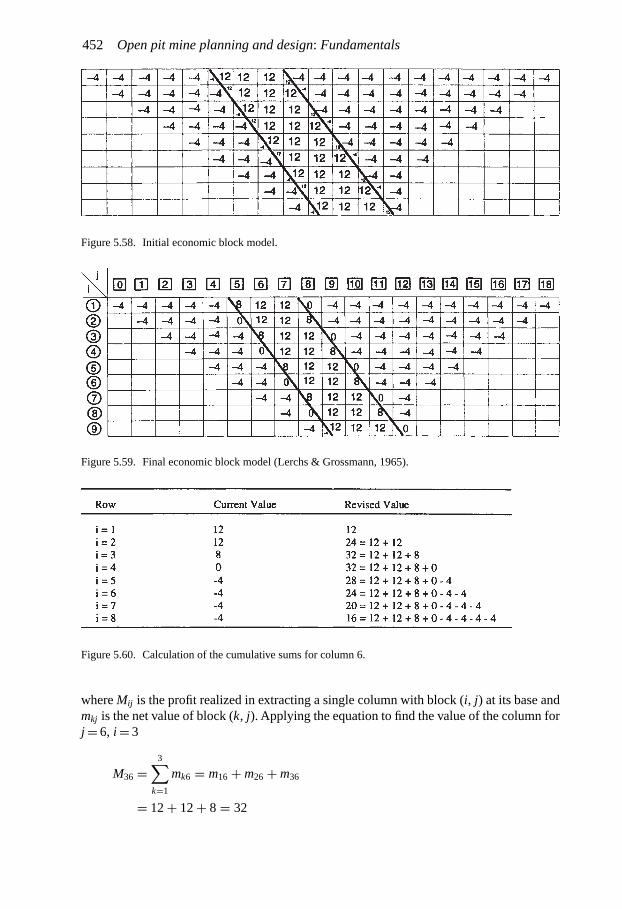
Figure 5.58. Initial economic block model.
Figure 5.59. Final economic block model (Lerchs & Grossmann, 1965).
Figure 5.60. Calculation of the cumulative sums for column 6.
where Mij is the profit realized in extracting a single column with block (i, j) at its base andmkj is the net value of block (k, j). Applying the equation to find the value of the column forj = 6, i = 3
M36 =3∑
k=1
mk6 = m16 + m26 + m36
= 12 + 12 + 8 = 32
Open pit mine planning and design: Fundamentals452

Figure 5.61. Completed cumulative sums (Lerchs & Grossmann, 1965).
The new table of values obtained by applying this process to all columns is shown in Figure5.61. The next step in the process is to add row i = 0 containing zero’s. A zero is also addedat position (i = 0, j = 0). This revised table is shown in Figure 5.61.
It is now desired to develop an overall cumulative sum as one moves laterally from leftto right across the section. Beginning with the extreme top left hand real block, the valuesof three blocks are examined:
1. One directly above and to the left.2. One on the left.3. One directly below and to the left.
Of the three, that block which when its value is added to the block in question yields themost positive sum is selected. An arrow is drawn from the original block to that block. Thissum is substituted for that originally assigned and becomes the value used for subsequentcalculations.
Figure 5.62 shows the process for block (1, 1). This process is continued, working downthe first column, then down the next column to the right, until all blocks have been treated. Itshould be pointed out that the reason some of the blocks on the section have not been filledin is that they fall outside of the bounds of the ultimate pit. Figure 5.63 shows the resultswhen the process has been completed through column 7.
One can examine the relationship between the values in the current table to the initialblocks (Fig. 5.59). If one follows the arrows beginning at the value 32, the pit which resultsis indicated by the shaded line (Fig. 5.64).
Superimposing the same pit on the block model one finds that the cumulative value of theblocks is 32 (Fig. 5.65). Moving up to the block containing the value 60 in Figure 5.64 onefollows the arrows to outline the pit. The value obtained by summing the blocks is also 60(Fig. 5.65). Therefore the technique provides a running total of the value of the pits definedby following the arrows. At this point in the calculation, the optimum pit has a value of 84.Figure 5.66 shows the results when the summing process is completed. The optimum pit isthat which has the maximum cumulative value. To determine this, one moves from right toleft along row 1 until the largest value is encountered. The arrows are then followed aroundto give the optimum pit outline on the section.
Pit limits 453pj
wst
k|40
2064
|143
5603
480

Figure 5.62. Procedure for determining the cumulative maximum value and maximizing direction.
Figure 5.63. Progression of summing process through column 7.
Open pit mine planning and design: Fundamentals454

Figure 5.64. Pit determination and total value by follow-ing the arrows.
Figure 5.65. Individual block values for the two partialpits.
Figure 5.66. The summing process has progressed through the entire section (Lerchs & Grossmann, 1965).
The pit is shown in Figure 5.67. The value is 108. The relationship between the values inFigure 5.67 and the actual block values can be seen by comparing Figures 5.67 and 5.68.
To complete the analysis one calculates:
Net value = 108 × $1000 = $108, 000
Total tons = 36 blocks × 10, 000 tons/block = 360, 000 tons
Tons ore = 20 blocks × 10, 000 = 200, 000 tons
Pit limits 455

Figure 5.67. Optimum pit determination.
Figure 5.68. Optimum pit limits superimposed on the block model.
Tons waste = 16 blocks × 10, 000 = 160, 000 tons
Stripping ratio = 16
20= 0.8
Average profitability/ton = $108, 000
360, 000= $0.30/ton
The expressions used (Lerchs & Grossmann, 1965) to calculate the ‘derived’ profit Pij (asgiven in Fig. 5.66) are
Pij ={
0, i = 0Mij + max
k=−1,0,1Pi+k,j−1 i �= 0 (5.16)
The maximum is indicated by a arrow going from (i, j) to (i + k, j − 1). Pij is the maximumpossible contribution of columns 1 to j to any feasible pit that contains (i, j) on its contour.If the element (i, j) is part of the optimum contour, then this contour to the left of element(i, j) can be traced by following the arrows starting from element (i, j). Any feasible pit mustcontain at least one element of the first row. If the maximum value of P in the first row ispositive then the optimum contour is obtained by following the arrows from and to the leftof this element. If all elements of the first row are negative, then no contour with positiveprofit exists.
Open pit mine planning and design: Fundamentals456

Figure 5.69. The floating cone used to evaluate the final pit limits.
Figure 5.70. Situation after floating down two rows.
Figure 5.71. Situation after floating down three rows.
This same section (Fig. 5.59) can be evaluated using the floating cone technique. The‘stepped’ cone of Figure 5.69 has been used to float over the section. Figures 5.70 through5.73 show the intermediate pits with the final pit given in Figure 5.74. As can be seen theresult is the same as when using the Lerchs-Grossmann approach. An advantage of thefloating cone procedure is that a variety of slope angles can be modelled.
As shown in Figure 5.75, one can also examine the pit limits by considering the lengthsalong the perimeter. Consider the left-hand side (LHS) of the pit. The horizontal segments
Pit limits 457

Figure 5.72. Situation after floating down four rows.
Figure 5.73. Situation after floating down five rows.
Figure 5.74. Situation after floating down six rows.
Figure 5.75. Pit resulting from the manual approach using the stripping curves.
Open pit mine planning and design: Fundamentals458

are considered first to determine the vertical position. When the pit is slightly above theknown true position, the sum of the horizontal segments is
−4 − 4 − 4 + 0 + 8 + 6 = +2
When it is slightly below than the sum is
−4 − 4 − 4 − 4 − 4 + 0 + 4 = −16
Examining the vertical segments to find the correct horizontal position is done next. Whenthe contour is slightly inside the correct position the sum is
−4 − 4 − 4 + 0 + 8 + 12 = +8
When it is slightly outside, the sum is
−4 − 4 − 4 − 4 − 4 + 0 = −20
Therefore the correct position is as given by the floating cone and Lerchs-Grossmannprocedures. The same procedure could be followed on the right hand side.
5.6 MODIFICATION OF THE LERCHS-GROSSMANN 2-D ALGORITHMTO A 2½-D ALGORITHM
The two-dimensional dynamic programming algorithm for determining the optimal con-figuration of blocks to be mined in cross-section was presented in the previous section.The technique is elegant yet simple. Like all other two-dimensional techniques it has thedrawback that extensive effort is usually required to smooth out the pit bottom and the pitends as well as to make sure that the sections fit with one another. As indicated by Johnsonand Sharp (1971), this smoothing seldom results in an optimal three-dimensional pit. Themodification which they proposed to the basic algorithm, as described in this section hasbeen referred to as the 2½-D algorithm (Barnes, 1982). An overall view of the block modelto be used is shown in Figure 5.76.
The column of blocks representing in the longitudinal section (i = 4, j = 1)
2 Level 1−3 Level 2
1 Level 3−7 Level 4
Figure 5.76. Block model used for the2½-D projection bound (Johnson & Sharp,1971).
Pit limits 459

This process is repeated for each of the other sections. The resulting longitudinal section isshown in Figure 5.79. The 2-D algorithm is now applied and the optimal contour becomesthat given in Figure 5.80.
Figure 5.77 shows the 5 sections of a block model. Beginning with section 1, the opti-mum pit outlines are determined, given that one must mine to a given level k. In this casethere are four levels to be evaluated. The results are shown in Figure 5.78. Each outline
Figure 5.77. Block sections for the 2½-D model (Johnson & Sharp, 1971).
Figure 5.78. Analysis of section 1.
Open pit mine planning and design: Fundamentals460

Figure 5.79. Longitudinal section (Johnson & Sharp, 1971).
Figure 5.80. Optimal longitudinal contour (Johnson & Sharp,1971).
is found using a slightly modified version of the Lerchs-Grossmann 2-D algorithm. Thenet values for each of the four pits on this section are then determined. As can be seenthese are:
Level 1: S11 = 2
Level 2: S12 = −3
Level 3: S13 = 1
Level 4: S14 = −7
To combine all of the transverse (ik) sections, a longitudinal section will now be taken. Inviewing Figure 5.78, it is seen that the deepest mining on section 1 ( j = 1) occurs at columni = 4. A column [i = 4, j = 1 (section 1)] of blocks will now be formed representing the netvalue of the cross-section as mined down to the various levels.
The net value for the material contained within the pit is found by summing the blockvalues along the final contour. Here it becomes
Pit value = 2 + 0 + 5 + 0 − 1 = 6
Now that the bottom levels for each of the transverse sections have been determined, onegoes back to these sections and selects the appropriate one. These are summarized inFigure 5.81.
The data and solution for a somewhat more complicated problem are given in Figures5.82 and 5.83, respectively. The block height to length ratio along the longitudinal section(the axis of mineralization) is 1 to 2 while for the cross-sections the block height and lengthare equal (1 to 1). Hence to maintain a maximum pit slope of 45 degrees, the pit slope canchange by two blocks per section along the length but by only block per column across thewidth.
Pit limits 461

Figure 5.81. Optimal longitudinal pitsections (Johnson & Sharp, 1971).
5.7 THE LERCHS-GROSSMANN 3-D ALGORITHM
5.7.1 Introduction
When evaluating final pit dimensions based upon reserves expressed in the form of a gradeblock model, the overall objective is to find a grouping of blocks such that a selectedparameter, for example:
– profit,– metal content, or– marginal value
is maximized. In preceding sections, some 2-dimensional approaches have been discussed.This is however a 3-dimensional problem and to obtain a true optimum such an approach isrequired.
For an orthogonal set of blocks there exist two basic geometries of interest forapproximating an open-pit. They are:
– the 1–5 pattern, where 5 blocks are removed to gain access to one block on the levelbelow and
– the 1–9 pattern, where 9 blocks are removed to gain access to one block on the levelbelow.
Open pit mine planning and design: Fundamentals462

Figure 5.82. Block sections for a more complicated example (Johnson & Sharp, 1971).
Pit limits 463

Figure 5.83. The solution for the Figure 5.82 block model (Johnson & Sharp, 1971).
Figure 5.84. Representation of the 1-5 and 1-9 block constraints (Laurent et al., 1977).
The geometric configurations and equivalent graphic representations for these two geome-tries are shown in Figure 5.84. The nodes represent the physical blocks. The arrows (directedarcs) point toward those blocks immediately above which must first be removed beforethe underlying block can be mined. Each block has a weight associated with it. In gen-eral, the weight assigned is equal to the value of the parameter being maximized. Often thisis the net economic value. The weight may be positive or negative.
Lerchs & Grossmann (1965) published the basic algorithm which when applied to a 3-Ddirected graph (block model) would yield the optimum final pit outline. This section presentsin a simplified way, the basic concepts. They are illustrated by examples.
Open pit mine planning and design: Fundamentals464

5.7.2 Definition of some important terms and concepts
There are a number of terms and concepts which are taken from graph theory (Lerchs &Grossmann, 1965; Laurent et al., 1977). The authors have tried to simplify them and yetretain their basic meaning.
Figure 5.85a is a section through a simple 2-D block model. As can be seen it consists of6 blocks.
Each block is assigned a number (xi) which indicates its location within the block model.In the case shown in Figure 5.85a, the block location are x1, x2, x3, x4, x5, and x6. Onewould know from the construction of the block model that the block designated as x1 wouldactually have center coordinates of (2000, 3500, 6800). If there were 100,000 blocks in theblock model, then xi would go from x1 to x100,000.
The file of node locations may be expressed by
X = (xi)
Figure 5.85b shows the 6 blocks simply redrawn as circles while maintaining their positionsin 2-D space. For the graph theory application each of these circles is now called a ‘node’.Straight line elements (called ‘edges’ in graph theory) are now added connecting the lowernodes to the nearest overlying neighbors. For the 3-D representations shown in Figure 5.84there would be 9 edges for each underlying block in the 1-9 model and 5 for the 1-5 model. Inthis 2-D model there are 3 edges for each underlying block. The nearest overlying neighborsfor node x5 as shown in Figure 5.85c are nodes x1, x2 and x3. The physical connection ofnode x5 to node x1 can be expressed either as (x5, x1) or (x1, x5). In Figure 5.85c, the nodeshave been connected by 6 edges:
(x1, x5) = (x5, x1)
(x2, x5) = (x5, x2)
Figure 5.85. Steps in the model buildingprocess.
Pit limits 465

(x3, x5) = (x5, x3)
(x2, x6) = (x6, x2)
(x3, x6) = (x6, x3)
(x4, x6) = (x6, x4)
These edges (eij) can be described by
eij = (xi, xj)
The set containing all edges is given the symbol E:
E = (eij)
A graph is defined as:
Graph: A graph G = (X, E) is defined by a set of nodes xi connected by ordered pairs ofelements called edges eij = (xi, xj).
The next step is to indicate which overlying blocks (nodes) must be removed prior toremoving any given underlying block (node). This adds the required sequencing (flow) fromthe lowest most to the upper most blocks (nodes). To accomplish this, arrows are attachedto the edges (lines) connecting the nodes (blocks) pointing in the direction of removal. Thishas been done in Figure 5.85d. By adding an arrowhead (direction) to an edge, the edgebecomes an arc,
akl = (xk , xl)
An arc denoted by (xk , xl) means that the ‘flow’ is from node xk to node xl (the arrowheadis on the xl end). The set containing all arcs in given the symbol A
A = (akl)
The graph (G) consisting of nodes {X} and arcs {A} is called a directed graph.
Directed graph: A directed graph G = (X , A) is defined by a set of nodes xl connected byordered pairs of elements akl = (xk , xl) called the arcs of G.
One can consider the entire set of nodes (blocks) and the arcs connecting them (thedirected graphs G(X , A)) or only a portion of it. A subset (Y ) is referred to as a directedsubgraph and represented by G(Y , AY ). An example of a directed subgraphs is shown inFigure 5.86. There are a great number of these subgraphs in the overall graph.
Subgraph: A directed subgraph G(Y ) is a subset of the directed graph G(X, A). It is madeup of a set Y of nodes and all of the arcs AY which connect them.
To this point in the discussion we have considered (1) the physical location of the blocksin space, (2) the connection of the blocks with one another and (3) the fact that overlying
Figure 5.86. Example of a subgraph.
Open pit mine planning and design: Fundamentals466

Figure 5.87. The weights assigned to theblocks of Figure 5.85.
blocks must be removed prior to mining lower blocks. Nothing has been said regardingthe values of the individual blocks. Each block (xi) has an associated weight (mi). This isshown in Figure 5.87 for the blocks in Figure 5.85a. Although we have used net value asthe assigned weight (mi) to this point in the book other measures of worth or content canalso be applied (profit, mineral content, etc.).
From a mining view point, the subgraph consisting of the four blocks. x1, x2, x3 and x5
could form a physically feasible pit. The subgraph consisting of blocks x2, x3, x4 and x6
could form another. A third possibility of a feasible pit is formed by the six blocks x1, x2,x3, x4, x5 and x6. There are many other feasible combinations. The subgraph x2, x3 and x6 isnot feasible since one of the overlying blocks x4 has not been included. The term ‘closure’is used to indicate a feasible subgraph.
Closure: Closure from the viewpoint of a mining engineer is simply a subgraph Y yieldinga feasible pit.
Each one of these feasible pits (subgraphs) has an associated total weight (value). Thechallenge for the mining engineer is to find that one pit (subgraph) out of the great manypossible which yields the maximum value. In graph theory this is referred to as finding thedirected subgraph of ‘maximum closure’.
Maximum closure: Again from the viewpoint of the mining engineer, maximum closure isthat closure set, out of all those possible, which yields the maximum sum of block weights,i.e. where MY = ∑
mi is a maximum.A procedure based upon the application of graph theory is used to identify and sort through
the various feasible pits in a structured way to find that yielding the maximum value. Thiscorresponds to the optimum pit. To better follow the discussion the following definitionsare introduced.
Circuit: A circuit is a path in which the initial node is the same as the find (terminal) node.
Chain: A chain is a sequence of edges in which each edge has one node in common withthe succeeding edge.
Cycle: A cycle is a chain in which the initial and final nodes coincide.
Path: A path is a sequence of arcs such that the terminal node of each arcs is the initial nodeof the succeeding arc.
To illustrate the process, a discussion based upon a tree analogy is used. The terms ‘tree’,‘root’, ‘branch’ and ‘twig’ are defined below:
Tree: A tree T is a connected and directed graph containing no cycles. A tree contains onemore node than it does arcs. A rooted tree is a tree with a special node, the root.
Root: A root is one node selected from a tree. A tree may have only one root.
Branch: If a tree is cut into two parts by the elimination of one arc akl, the part of the treenot containing the root is called a branch. A branch is a tree itself. The root of the branch isthe node of the branch adjacent to the arc akl.
Pit limits 467

Figure 5.88. Example of a branch.
Figure 5.89. Example to be worked using the Lerchs-Grossmann 3-D algorithm.
Each arc akl of a tree T defines a branch Tkl. The weight Wkl of a branch Tkl is the sum ofall weights associated with nodes of Tkl. An example of a branch is shown in Figure 5.88.
Twig: A twig is a branch of a branch.
As ‘twigs’ and ‘branches’ are added or cut from the ‘tree’, the value of the tree changes.The Lerchs-Grossman algorithm is based upon a normalizing procedure in which a
number of rules are followed. These will be demonstrated in detail in the next section.
5.7.3 Two approaches to tree construction
The algorithm starts with the construction of an initial tree T 0. This tree is then transformedinto successive trees T 1, T 2, . . . , Tn following given rules until no further transformation ispossible. The maximum closure is then given by summing the nodes of a set of well identifiedbranches of the final tree. There are two approaches which may be used for generating theinitial tree.
Approach 1. Construct an arbitrary tree having one connection to the root.
Approach 2. Construct a tree with each of the nodes connected directly to the root.
The simplest of these is Approach 2. Both approaches will however be applied to the simpleexample shown in Figure 5.89.
Although elementary, this is an interesting problem since the floating cone approachwould suggest no mining at all. By inspection however one would strip the four waste
Open pit mine planning and design: Fundamentals468

Figure 5.90. Addition of a root.
Figure 5.91. Labelling of plus and minus arcs.
blocks to uncover the two ore blocks. The net value for the resulting pit is expectedto be +4.
The step-by-step approach used to demonstrate the techniques involved has been adaptedfrom that presented by Laurent et al. (1977).
5.7.4 The arbitrary tree approach (Approach 1)
This approach (including the common normalizing procedure used with both Approaches 1and 2) will be presented in step-by-step fashion.
Step 1. Begin by adding a root node x0 to the directed graph and construct a tree of yourchoice keeping in mind the connection possibilities
From node x5 : (x5, x1)
(x5, x2)
(x5, x3)
From node x6 : (x6, x2)
(x6, x3)
(x6, x4)
The one chosen is shown in Figure 5.90. Each of the nodes (blocks) is connected to one ofthe others by a directed arc (arrow). One node is attached to the root.
Step 2. Each of the arcs is labelled with respect to whether it is directed away from the root(plus) or towards the root (minus). This is done in Figure 5.91.
Pit limits 469

Table 5.15. Labelling guide for arcs.
Case Direction Cumulative weight Label
1 Plus Positive Strong2 Plus Null or negative Weak3 Minus Positive Weak4 Minus Null or negative Strong
Figure 5.92. Labelling of weak and strong arcs.
Figure 5.93. Creation of tree T1.
Step 3. Beginning at the extremities each branch is worked back toward the trunk, summingthe weights supported by the individual arcs. The objective is to add the words ‘strong’ or‘weak’ to each of the arcs. Table 5.15 summarizes the labelling criteria.
We will begin on the left hand side of the tree. Roman numerals have been used to denotethe segments for the discussion. For arc I, the direction is plus and the weight is negative.Thus the label to be attached is ‘weak’ (Case 2). For arc II, the same is true. For arc V,the direction is plus and the weight negative. The label is weak. It is also Case 2. Whenexamining arc IV, the direction is minus and the cumulative weight is positive (10 − 4 = 6).Thus the label is weak (Case 3). Continuing to arc III, the direction is plus and the cumulativeweight is positive (10 − 4 − 4 = 2). The label is ‘strong’ (Case 1). Figure 5.92 presents theresulting direction and label for each arc of this initial tree.
Step 4. The figure is now examined to identify strong arcs. Two actions are possible:
Action 1. A strong-minus arc: The arc (xq, xr) is replaced by a dummy arc (x0, xq). Thenode xq is connected to the root.
Action 2. A strong-plus arc: The arc (xk , xl) is replaced by the dummy arc (x0, xl). The nodexl is connected to the root.
In this example there is one strong arc III. Since it is a ‘strong-plus’ arc, action 2 is taken.The arc connecting node x5 (10) to node x3 (−4) is removed. An arc connecting the root x0
to node x3 (−4) is drawn instead (Fig. 5.93). This becomes tree T 1.
Open pit mine planning and design: Fundamentals470

Figure 5.94. Tre1e T1 with labels attached T0
arcs.
Figure 5.95. Initial tree with all root connection.
Step 5. Tree T 1 is examined in the same way as before labelling the arcs as to whether theyare ‘plus’ or ‘minus’ and ‘weak’ or ‘strong’. This has been done in Figure 5.94.
Step 6. Any strong branches of the new tree not directly connected to the root are identifiedand the procedure discussed in Step 4 is followed. If there are no strong branches notconnected to the root, the tree is said to be normalized and the process is over.
Step 7. The maximum closure consists of those nodes connected by strong arcs to the root.In this case the closure is
−4 − 4 + 10 − 4 − 4 + 10 = +4
5.7.5 The all root connection approach (Approach 2)
The step-by-step procedure is outlined below.
Step 1. Begin by adding a root node and connecting arcs between the root and each of theother nodes. For the example problem, this initial tree T 0 is shown in Figure 5.95. Note thatall of the arcs are ‘plus’.
Step 2. The set (graph) of directed arcs is now split into two groups. Those connected tothe root by strong-plus arcs are included in group Y 0. The others are in group X-Y 0. In thiscase nodes x5 and x6 are in group Y 0. Their sum is 20.
Step 3. One must now look at the possible connections between the two groups. Followingthe sequencing constraints there are 6 directed arcs which can be drawn:
For x5: (x5, x1)
(x5, x2)
(x5, x3)
Pit limits 471

Figure 5.96. Selection of directed arc (x5, x1).
Figure 5.97. Labelling of the resulting arcs.
For x6: (x6, x2)
(x6, x3)
(x6, x4)
One of these is selected. In this case it will be the connection (x5, x1). The directed arc(x0, x5) is removed and the directed arc (x5, x1) drawn. This is shown in Figure 5.96.
Step 4. The normalizing process is now followed. Each arc is labelled with respect to ‘plus’or ‘minus’ and ‘strong’ or ‘weak’. The result is shown in Figure 5.97. The arc(connection)between x0 and x1 is still strong-plus. Hence the members of the Y group are x1, x5 and x6.The value of Y (closure) is 16.
Step 5. One now returns to step 3 to seek additional connections between the Y and X-Y(X without Y ) groups. There are 5 feasible arcs
(x5, x2)
(x5, x3)
(x6, x2)
(x6, x3)
(x6, x4)
The arc (x5, x2) will be added to the tree and arc (x0, x2) dropped. This is shown in Figure 5.98.
Open pit mine planning and design: Fundamentals472

Figure 5.98. Addition of arc (x5, x2) and droppingarc (x0, x2) from the tree of Figure 5.97.
Figure 5.99. Labelling of the resulting arcs.
Figure 5.100. Addition of arc (x6, x3) and drop-ping arc (x0, x3) from the tree of Figure 5.97.
Step 6. The new tree is now normalized. The result is shown in Figure 5.99. The nodesincluded in Y are x1, x2, x5 and x6. The closure Y is 12.
Step 7. Returning to Step 5, there are now 3 possible connections remaining:
(x5, x3)
(x6, x3)
(x6, x4)
Here we will choose to add arc (x6, x3) and drop arc (x0, x3). (The choice (x5, x3) is aninteresting one and will be evaluated later.) The resulting normalized tree is shown in Figure5.100. The arc (x0, x6) remains strong-plus and hence the nodes included within Y are x1,x2, x3, x5, and x6. The overall closure is 8.
Step 8. Returning to Step 5 there is one possible connection remaining: arc (x6, x4). Arc(x0, x4) is dropped and arc (x6, x4) added. The tree is normalized as before with the result
Pit limits 473

Figure 5.101. Addition of arc (x6, x4) and droppingarc (x0, x4).
Figure 5.102. The resulting normalized tree for thealternative when arc (x5, x3) is added and arc (x0, x3)is dropped.
given in Figure 5.101. All of the nodes are now attached directly to the root by chains havingone strong edge. There are no more connections to be tried.
Step 9. The maximum closure now is the cumulative sum of the nodes involved. In this caseit is +4.
As was indicated, at the stage shown in Figure 5.98, it is possible to select connection(x5, x3). We will now return to this point and consider this option.
Step 7*. Arc (x5, x3) will be added and arc (x0, x3) dropped. The normalized tree is shownin Figure 5.102. As can be seen, the arc (x0, x1) has now become weak-plus.
The only member of the Y group is now x6. The closure is 10.
Step 8*. One now considers the possible connections between the X-Y and Y groups. Thereare two possibilities.
(x6, x4)
(x6, x3)
Selecting (x6, x3) one obtains the normalized tree in Figure 5.103. The members of the Ygroup are x6 and x4. The closure is 6.
Step 9*. There is one possible connection between the two groups, that one being througharc (x6, x3). For the tree in Figure 5.104, arc (x0, x1) has been dropped and arc (x6, x3) added.The normalized tree is shown. As can be seen all of the nodes are connected to the rootthrough a chain containing one strong edge. There are no more possible connections. Theclosure is the sum of the nodes which is +4.
Open pit mine planning and design: Fundamentals474

Figure 5.103. Normalized tree for connectingarc (x6, x3).
Figure 5.104. Normalized tree when adding arc (x6,x3) and dropping arc (x0, x1).
Figure 5.105. The example used to demonstrate tree cutting.
Figure 5.106. The arcs added to form the initial tree.
5.7.6 The tree ‘cutting’ process
The preceding problem was a simple case intended to familiarize the reader with thealgorithm. In this example, the process of ‘cutting’ the tree during normalization will bedemonstrated. The problem is as shown in Figure 5.105. The initial tree is as shown inFigure 5.106.
Pit limits 475

Figure 5.107. The normalized tree after 4iterations.
Figure 5.108. The arc (x0, x3) is dropped and arc(x6, x2) added.
Figure 5.109. The arc (x5, x3) is cut and the arc (x0, x2)added.
The initial choices for connection are the same as before. They will be done in thefollowing order:
For x5: (x5, x1)
(x5, x2)
For x6: (x6, x3)
(x6, x4)
After these 4 iterations the normalized tree would appear as in Figure 5.107.The Y group is shown to consist of nodes x3, x4 and x6. There is one remaining connection
to be made between the groups (x6, x2). In Figure 5.108, arc (x0, x3) is dropped and arc(x6, x2) added. The tree is then normalized. As can be seen the arc (x5, x2) is strong-plus andnot connected directly to the root. It must be cut in order to normalize the tree.
As discussed earlier the arc (xk , xl) is replaced by the dummy arc (x0, xl). In this casexk = x5, xl = x2. Thus the new arc is (x0, x2). This is shown in Figure 5.109. The resultingtree is in normalized form. All of the connections have been tried. The final closure is20 − 10 − 2 − 2 = +6. It can be seen that if Case 1 in Table 5.15 had been written as
Open pit mine planning and design: Fundamentals476

‘cumulative weight = null or positive’ rather than just as ‘cumulative weight = positive’,then both nodes x1 and x5 would have been included in the maximum closure as well.
5.7.7 A more complicated example
Figure 5.110 shows a more complicated directed network to be analyzed using the Lerchs-Grossmann algorithm (Laurent et al., 1977). The results are shown in Figure 5.111. Theinterested reader is encouraged to select the upper two layers to work as an exercise. As canbe seen, the two blocks at the pit bottom +10 and −10 would contribute a net of 0 to thesection value and hence have not been mined.
Figure 5.110. A more complicated example on which to practice the algorithm (Laurent et al., 1977).
Figure 5.111. Maximum closure for the more complicated example (Laurent et al., 1977).
Pit limits 477

5.8 COMPUTER ASSISTED METHODS
5.8.1 The RTZ open-pit generator
Fairfield & Leigh (1969) presented a paper ‘A computer program for the design of open-pits’, which outlines a pit planning procedure in use by many mines today. This sectionwill describe, using the material of Fairfield & Leigh (1969), the basic logic involved. Thecomputer techniques using sections do not solve the problem of end sections or the smoothingof perimeters and consequently have definite limitations. The projection of volumes in theform of cones also has some of the same limitations. The approach described here is theprojection of plan areas, specifically the projection of perimeter outlines.
The process begins with the development of a block model. Each block as a minimumwould be assigned location coordinates and an index character dependent on the rock typeor grade type.
The second step in the process is the selection of one or more base perimeters from whichto generate the pit. These define the final horizontal extent of the pit at, or close to, theelevation of the pit’s final base. Each perimeter so drawn becomes the trial base from whichan overall pit is generated.
The information that is required to carry out these calculations is:1. Size and shape of ore body.2. Ore and rock types present.3. Grades of ore.4. Rock slope stability.5. Size and shape of base perimeter.6. Cutoff grades.7. Depth of pit.8. Unit working costs.
The trial base perimeter is defined by a series of short chords (Fig. 5.112).The coordinates of the chord end points are read manually and then entered into the
computer or are read and entered directly using a digitizer. Such a file of clockwise readperimeter points is given in Table 5.16.
At every horizon, proceeding in a clockwise order, each defining perimeter chord isconsidered in turn. For each, the defining end coordinates are located.
To illustrate the basic method, consider the portion of the pit base defined by chords H1I1
and I1J1 shown in Figure 5.113.
Base Perimeter Chord l
Point (l)
Point (l + 1)
Figure 5.112. Trial based perimeter(Fairfield & Leigh, 1969).
Open pit mine planning and design: Fundamentals478

The coordinate pairs H1, I1 and J1 are projected outwards and upwards to the next upperhorizon in a direction normal to the perimeter at that point. The next upper horizon occursat a specified distance above the current horizon. The actual interval is determined by therequirements of the job at hand and is some fractional part (usually one-half) of the benchheight. The slope angle used is that permitted in the particular rock type or at that pit position.
Table 5.16. Perimeter coordinates* for trial base (Fairfield & Leigh, 1969).
Perimeter coordinates
Y X Y X Y X Y X
445.2 601.8 420.5 619.0 404.3 641.7 391.7 659.4394.3 681.2 397.2 705.8 401.2 726.7 408.6 746.3410.0 768.1 415.6 796.4 424.6 817.9 428.5 843.3428.7 869.6 424.5 888.0 432.1 916.6 428.4 945.3437.0 969.0 415.6 984.7 393.5 1001.5 378.6 1021.8369.7 1050.1 371.4 1077.4 378.7 1106.8 382.8 1130.0382.8 1150.3 382.8 1170.8 382.8 1195.7 395.4 1212.5408.1 1229.5 420.5 1246.0 434.0 1264.0 447.3 1281.7468.7 1287.3 490.6 1292.9 516.1 1298.5 546.1 1305.2569.3 1299.1 502.9 1292.0 616.3 1280.2 640.4 1265.8668.2 1242.7 681.3 1228.7 695.1 1214.9 716.2 1193.8727.9 1166.9 746.5 1147.0 763.6 1125.1 776.1 1101.4783.7 1075.3 783.0 1048.0 770.0 1027.6 754.6 1008.0757.4 984.5 751.0 958.6 748.8 933.5 744.7 912.9742.4 884.9 744.9 864.6 755.4 841.3 760.6 810.1756.9 789.2 752.9 766.9 741.7 749.0 723.7 726.2706.5 711.6 682.8 693.9 661.7 679.5 647.0 667.9631.1 652.4 619.9 631.5 610.7 610.1 594.9 597.2571.7 575.8 547.3 559.6 512.2 562.4 488.3 578.3464.3 598.4
* Coordinate pairs are connected reading from left to right and top to bottom in the table.
Figure 5.113. Projection of chords and perimeter points along the bisectors (Fairfield & Leigh, 1969).
Pit limits 479

If the slopes at the chord ends are different then the mean value is used.
Slope of chord I = 1
2(permitted slope at point (I)
+permitted slope at point (I + 1)) (5.17)
Sufficient information is now available:(i) the coordinates of the chords defining the current perimeter,(ii) the average permitted rock slopes of these chord locations,
(iii) the elevation difference to the next upper horizon,to generate the pit perimeter on the next upper horizon. With this information the programworks clockwise around the perimeter, considering pairs of adjacent chords in turn.
Consider the case where adjacent chords HI and IJ have the same permitted rock slopesθ and I is to be projected from Horizon 1 to Horizon 2 through a vertical height V . Thesituation is shown in plan in Figure 5.113 and in isometric view in Figure 5.114.
The calculation of the new coordinates of I on level 2 (I2) is given below:
Bisector of angle H1I1J1 = −→I1A
Length of I1A = V cot θ
Bearing angle of I1A = α
New coordinates of I2 = (x1 + dx, y1 − dy)
= (x1 + I1A sin α, y1 − I1A cos α)
As an example assume that
θ = 45◦
V = 10 m
x1 = 510.36
y1 = 840.98−→I1A = N50◦E
α = 50◦
The horizontal distance I1A is given by
I1A = V cot θ = 10 cot 45◦ = 10 m
Figure 5.114. Isometric projection of chord HI(Fairfield & Leigh, 1969).
Open pit mine planning and design: Fundamentals480

Figure 5.115. Isometric projection of adjacentchords HI and IJ (Fairfield & Leigh, 1969).
Using the bearing angle, one can calculate the distances dx and dy.
dx = I1A sin α = 10 sin 50◦ = 7.66
dy = I1A cos α = 10 cos 50◦ = 6.43
Hence the coordinates (x2, y2) of I2 become
x2 = x1 + dx = 510.36 + 7.66 = 518.02
y2 = y1 − dy = 840.98 − 6.43 = 834.55
When adjacent chord slopes are not the same, (Fig. 5.115) an ‘averaging’ method is used inorder to smooth out sharp changes in slope.
(i) The rock slope of any chord is the mean of the slopes as obtained at the chord end points.
For chord H1I1, slope = θb = 1
2(θh + θi)
For chord I1J1, slope = θd = 1
2(θi + θj)
(ii) The horizontal distance IA (whereA is the midpoint ofA′A′′) is the mean of the distancesBC and DE.
Since
B1C = V cot θb
D1E = V cot θd
Then
I1A = 1
2(B1C + D1E)
or
I1A = 1
2V
(cot
θh + θi
2+ cot
θi + θj
2
)
Pit limits 481

Orebody Axis
Strip
Block Grid
#1
#2
#3
NewPerimeter
Figure 5.116. Superposition of the bench perimeters onthe block model.
The new coordinates of I2 are given by
New coordinates of I2 = (x + I1A sin α, y − I1A cos α)
The program then continues around the perimeter and considers each pair of chords in turnand calculates the coordinates of the projected chord end points on the next upper horizon.
When the perimeter on the next upper horizon has thus been generated, the area lyingwithin the new perimeter is scanned and, by reference to the rock type matrix and appropriatevertical interval, the volumes and tonnages of the various rock types between the lower andupper horizons are calculated. The principle adopted is analogous to that of obtaining areasby graph paper rather than by planimeter. Volumes are calculated down to the previoushorizon on which a perimeter was generated.
The program works around the perimeter and considers each chord in turn. For eachchord, the elemental area between the chord and the axis of the ore body is evaluated interms of the types of rocks falling within the strip (see Fig. 5.116).
By referring to the current rock matrix as stored in the ‘memory’of the computer, the zonebetween the chord and axis is scanned. Each rock type present is identified and counted interms of blocks. Then, by reference to the cell dimensions and the level interval, the numberof blocks is converted into a volume. In this way all the elements within the pit perimeterare evaluated and progressive totals of each rock type are built up. Table 5.17 shows thetype of output which is obtained.
Before continuing to project the perimeter up to the next horizon two checks are madeand adjustments carried out if necessary. First the perimeter chords are checked to ensurethat the chord length is maintained within a specific range. If the chord length exceedsa certain permitted maximum, an intermediate coordinate point is introduced at the chord’smid point. On the other hand, in certain circumstances, the chord length may become verysmall and on further projection the end points may actually reverse their order. This will giverise to ambiguous calculations resulting in a badly distorted perimeter, so in order to avoidthis situation points are dropped out as chord lengths become less than a certain permittedminimum. The program then scans the perimeter and checks for the development of sharpangles between adjacent perimeter chords, which are compared with a given minimum angle(set with the input data). If the acute chord angle is too sharp, perimeter points are adjusteduntil the angle becomes larger than the permitted minimum. This part of the program obviatesthe problem of the development of sharp pit-perimeter curves.
Open pit mine planning and design: Fundamentals482

Table 5.17. Typical bench output using the RTZ pit generator (Fairfield & Leigh, 1969).
Test case 3Base perimeter : 720 ftBench No: 11 (Elevation = 440 ft)Footwall slope angle = 45◦Hangingwall slope angle = 55◦
Rock type 1 2 3 4 5 6 7 8
Area (ft2) 4423.4 29,537.0 59,059.9 45,353.7 14,685.8 1440.0 73,175.6 0.0Volume (ft3) 146,627.0 998,383.0 1,793,687.0 1,674,718.0 358,986.0 29,038.0 2,327,491.0 0.0
Total area = 227,675.8 ft2
Total volume = 7,328,930 ft3
Table 5.18. Typical total pit output using the RTZ pit generator (Fairfield & Leigh, 1969).
Test case 3: Final summaryBase perimeter : 720 ftFootwall slope angle: 45◦Hangingwall slope angle: 55◦
Rock type 1 2 3 4 5 6 7 8
Volume (ft3) 3,348,438 5,979,359 17,496,752 13,867,850 9,031,000 1,029,359 51,243,824 7,470,351Tonnage 304,403 519,944 1,458,062 1,109,428 694,692 76,249 3,660,273Cutoff grade (%) 0.6 0.5 0.4 0.3Volumetric stripping ratio W : O 10.0 2.8 1.5 1.1Total tonnage of ore (tons) 824,347 2,282,409 3,391,837 4,086,529Total tonnage of waste (tons) 6,998,704 5,540,642 4,431,214 3,726,522Average mill feed grade (%) 0.64 0.55 0.50 0.47Total working costs (units) 27,143,601 32,642,173 34,924,076 36,024,585
Having carried out these checks the program continues to the next horizon where thecomplete cycle is repeated. Then so on until the final pit perimeter is reached.
Table 5.18 is a typical final summary output from the program. The following are given:(i) Pit perimeter coordinates.
(ii) Volume and tonnage of ore.(iii) Volume and tonnage of waste.(iv) Stripping ratio.(v) Average grade of mill feed.
(vi) Total working costs.In cases where working costs and revenues are required additional input to the computer isnecessary. Costs are fed in under headings: ‘fixed costs per rock type unit’ (that is, drilling,blasting, loading), ‘depth variable costs’ (that is, transport from various working levels),and ‘fixed cost per unit of rock’ (that is, supervision, services).
The basic pit design method described so far develops a single pit from a single base.Having completed a design for a single pit, the user can continue to add on additional pitseither as incremental expansions to the first pit by incorporating a new base which joins the
Pit limits 483

Working Pit
First Pit
First Pit Second Pit
Extension toWorking Pit
A. Extension to Working Pit
B. Incremental Expansions
Increments
C. Double Base Pit
Figure 5.117. More complicated pit expansions (Golder Associates, 1981).
first pit, or by specifying a second base lying outside the first pit thereby creating a doublebase pit. The same procedure is adopted. A trial base perimeter for the second pit is input tothe computer in the same form, and the program repeats the cycle of projection from levelto level until the surface is reached.
The perimeter of this second pit will probably encroach on that of the first pit. However,with the aid of its memory the computer will take into consideration the fact that one pit hasalready been generated. As soon as encroachment occurs the complete volume bounded bythe first pit perimeter will be treated as being mined out and hence air. This prevents anyduplication that would otherwise occur. Third and further bases can be added by similarmeans. A second or further base can represent:
1. A working extension to the first pit (Fig. 5.117A).2. An incremental expansion of the pit to test the sensitivity of the first pit to profitability
(Fig. 5.117B).3. A second pit which may merge with the first at the upper benches (Fig. 5.117C). A
typical computer assisted pit design is shown in Figure 5.118.
5.8.2 Computer assisted pit design based upon sections
Open-pit design computerization which began in the early 1960’s was driven largely bythose involved in the mining of large, low grade deposits. The choice of a block model to
Open pit mine planning and design: Fundamentals484

Figure 5.118. A typical pit design (Motta, 1988).
represent porphyry copper deposits, for example, was appropriate. The block size could bemade still quite large and yet be small with respect to the size of the deposit and the scaleover which the major grade changes take place. The distinction between ore and waste wasmade on the basis of cut off grade rather than on a sharp boundary.
There are a number of applications where block models are less satisfactory. Steeplydipping, relatively narrow vein/strata form deposits being one example. Here the ore iscontained within definite, well defined boundaries. Grade variation within the ore zone issuch that an average ore grade may be assigned. In such cases, the use of vertical sections stillplays an important role. One computer assisted technique for dealing with such situationshas been described by Luke (1972). The example which he presented forms the basis forthis section.
Figure 5.119 illustrates the topography and geologic interpretation of a single cross-section through a steeply dipping iron orebody. A thin layer of overburden (alluvium, sand,gravel) overlies the bedrock. There is a sharp transition between the ore zone and the adjacenthanging- and footwall waste zones.
In the manual method of pit design using sections described in an earlier section, it willbe recalled that the final pit limits were obtained through an iterative process by which thepit shape was ‘floated’ around on the section until the actual stripping ratios and average oregrades matched a point on the SR-grade curve.
Such a trial pit for this section is shown in Figure 5.120. The pit bottom has a width of120 ft, the slope of the right hand slope (RHS) is 60◦ whereas the left hand slope (LHS)is reduced to 57◦ to include the presence of a 60 ft wide ramp segment. The straight lineapproximations for the slopes are used to simplify the process. Once the ‘final’ best positionis determined then the functional mining parameters such as:
– the ramp(s),– working bench heights,
Pit limits 485

Cross Section 196Y
1100
1000
900
800
700
600
500
Ele
vatio
n (f
t)
Rock Ore Rock
5200 5400 5600 5800 6000X
Easting (ft)
Overburden
Figure 5.119. Topography and geologic interpretation of a single cross-section for a steeply inclined orebody(Luke, 1972).
Cross Section 196Y
1100
1000
900
800
700
600
500
5200 5400 5600 5800 6000Easting (ft)
Ele
vatio
n (f
t)
X
Rock Ore Rock
PreliminaryPit Design
Figure 5.120. Preliminary pit design for example cross-section (Luke, 1972).
– berm widths, and– bench face angles
are added (Fig. 5.121).The design is then reexamined. Often significant changes occur between the simplified
and actual pit designs. When the ‘final’ design on this section has been located, the areas of
Open pit mine planning and design: Fundamentals486

Cross Section 196
1100
1000
800
600
700
900
500
5200 5400 5600 5800 6000
Y
X
Easting (ft)
Ele
vatio
n (f
t)
Rock Ore Rock
Ramp
Figure 5.121. Preliminary pit design for example cross-section (Luke, 1972).
overburden, ore and waste are obtained by planimetering. Overall stripping ratios, etc. canthen be calculated.
Design changes such as varying– minimum pit width,– slope angles,– position/width of the ramp, and– limiting stripping ratio
would require the entire process to be repeated.Computer techniques have been developed to assist in the preparation of the sections
and in making the necessary calculations. In this way a large number of potential designscan be evaluated quickly and inexpensively. Since the procedure largely follows the manualprocess, it is easy for the mine planner to understand what the program is accomplishing andto actively participate in computer-assisted design. The output of the process is a functionalmine plan together with a working set of cross-sections. This section will discuss via aniron-ore example, originally presented by Luke (1972) the logic involved in the process.
The process begins with a description of the topography and the geologic data. Thetopographic relief and the overburden-bedrock contact are defined by a series of straightline segments. The end points of each segment making up the individual contour line (string)are defined either by hand or using a digitizer. In this case the surface relief will be denotedas the surface contour and the top of bedrock as the overburden contour. The values forcross-section 196 are given in Table 5.19.
From the cross-section (Fig. 5.119) it is seen that there are four material types present.Since they adjoin one another, they can be defined by four zones. If, for example, a podof hangingwall waste exists in the ore then five zones would be needed. These zones mustbe described. In this simple case the ore-footwall and ore-hangingwall contacts can bedescribed using end point coordinates (Table 5.20).
Pit limits 487

Table 5.19. Surface and overburden contour strings for cross-section 196 (Luke, 1972).
Surface contour Overburden contour
X Y X Y
4870 1100 4870 10975000 1106 5000 11035114 1125 5111 11225251 1114 5222 11135298 1114 5305 11105416 1102 5406 11005539 1073 5419 11005613 1050 5523 10735673 1024 5590 10525723 1021 5710 10105743 1020 5770 10085838 1035 5842 10235940 1034 5940 10286000 1043 6057 10436100 1050 6121 10436121 1049 6200 10306200 1035
Table 5.20. End points for zone lines (Luke, 1972).
X1 Y1 X2 Y2
Ore-footwall contact 5298 1112 5550 440Ore-hangingwall contact 5558 1065 5787 440
Table 5.21. Material descriptors (Luke, 1972).
Zone Material type Material description Divisor
1 50 Rock waste 27.02 1 Ore 11.53 50 Rock waste 27.04 51 Overburden 64.8
The overburden zone lies between the surface and the overburden contour lines. Thefootwall (hangingwall) waste zone lies to the left (right) of the ore-footwall (hangingwall)zone line and below the overburden contour line. The ore zone lies between the contact linesand beneath the overburden contour line. Each zone corresponds to a particular materialtype which in turn has certain properties. In this case the area of each material includedin the pit will first be determined. This will be changed to a volume by multiplying by thegiven section thickness (i.e. 100 ft). To convert this volume into the desired units of tons,cubic yards, cubic yards of equivalent rock, etc., certain factors are required. A table of suchfactors is given in Table 5.21. In this case the factor of 11.5 is used to convert volume (ft3)
Open pit mine planning and design: Fundamentals488

Table 5.22. Pit wall specifications (Luke, 1972).
Bench Berm Wall Valid Overburden angle Toe coordinatesheight width angle berm
elevation X Y
Left 80 35 82 1000 45◦ 5500 680Right 80 35 82 1000 45◦ 5620 680
into long tons of crude ore. The factor of 27 converts volume (ft3) into cubic yards of rockwaste. Since the overburden is much easier to remove than the rock waste, a factor of 2.4is first introduced to convert volume of overburden (ft3) into an equivalent volume (ft3) ofrock waste. The factor of 27 is then used to convert ft3 into yd3. The overall factor is theproduct of these two (64.8).
The pit design can now be superimposed upon the basic material-geometry model. Asdone earlier the pit is defined by a series of connected straight segments. The width andposition of the pit bottom is first decided. For Figure 5.120 one can see that the width is120 ft and the bottom elevation is 680. The end points of this segment form the toe positionsof the left and right hand slopes. The walls are defined by:
1. Bench height. The bench elevation differential on the ultimate wall.2. Bench width.3. Wall angle. The bedrock wall angle from bench to bench, not the overall slope angle.4. Valid bench elevation. The elevation of any existing berm if the pit is under current
development, or the elevation of the first proposed bench. From this specified bench, theelevation of successive benches is determined from the bench height.
5. Overburden angle. The wall angle that can be maintained in overburden.6. Toe position. The (X, Y ) coordinates for the indicated intersection of the pit wall and
pit floor.The wall and pit bottom specifications for the trial pit are given in Table 5.22. The design
specifies the location of the ramp as to– left or right wall,– ramp elevation when it crosses the section, and– ramp width,
For the section shown it has been decided that the ramp should have
location = left wall,
elevation = 896 ft, and
width = 60 ft.
In manually superimposing the pit onto the section, the designer would locate the pit bottomand then using scale and protractor construct the pit walls. The ramp would be positioned atthe proper location. The same procedure is followed with the computer except that end pointcoordinates of the segments are determined. In addition, the coordinates of the intersectionsbetween the string making up the pit and the zone/contour lines are determined as well.Once this has been done, the areas involved in each zone can be obtained. For the ore zone(Zone 2) using a planimeter one might start in the lower left corner (Fig. 5.122) and proceedaround the loop in a clockwise motion eventually returning to the starting corner.
Pit limits 489

Cross Section 196
1100
1000
800
600
700
900
500
5200 5400 5600 5800 6000
Y
X
Easting (ft)
Ele
vatio
n (f
t)
Rock Ore Rock
1
4
32
Figure 5.122. Summary of developed data for the example cross-section (Luke, 1972).
Cross Section 196
1100
1000
800
700
900
5200 5400 5600 5800
Y
Easting (ft)
Ele
vatio
n (f
t)
Rock Ore Rock
8
9
10
76
45
32
1
1615
17
11
12 13
14
Figure 5.123. Ore area calculation based on the segment end points.
The same basic process is followed knowing the end point coordinates of the segments.Figure 5.123 shows the end point locations and Table 5.23 gives the coordinates.
To demonstrate the process by which areas are found consider the area excavated (A)from the bottom bench in Figure 5.124. The formula used is
A = 1
2(Y2 + Y1)(X2 − X1)
where Y1, X1 are coordinates of initial point of segment and Y2, X2 the coordinates of finalpoint of segment.
Open pit mine planning and design: Fundamentals490
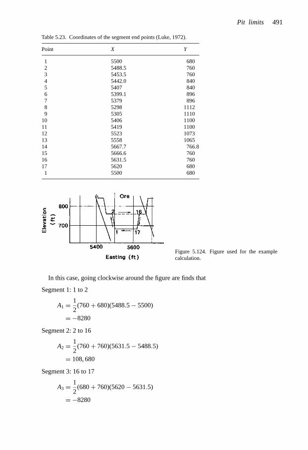
Table 5.23. Coordinates of the segment end points (Luke, 1972).
Point X Y
1 5500 6802 5488.5 7603 5453.5 7604 5442.0 8405 5407 8406 5399.1 8967 5379 8968 5298 11129 5305 1110
10 5406 110011 5419 110012 5523 107313 5558 106514 5667.7 766.815 5666.6 76016 5631.5 76017 5620 6801 5500 680
Figure 5.124. Figure used for the examplecalculation.
In this case, going clockwise around the figure are finds that
Segment 1: 1 to 2
A1 = 1
2(760 + 680)(5488.5 − 5500)
= −8280
Segment 2: 2 to 16
A2 = 1
2(760 + 760)(5631.5 − 5488.5)
= 108, 680
Segment 3: 16 to 17
A3 = 1
2(680 + 760)(5620 − 5631.5)
= −8280
Pit limits 491

Segment 4: 17 to 1
A4 = 1
2(680 + 680)(5500 − 5620)
= −81, 600
The total area is
A = A1 + A2 + A3 + A4 = −8280 + 108, 680 − 8280 − 81, 600 = 10, 520 ft2
Using the formula for the area of the trapezoid one finds that
Atz = 1
2(b1 + b2)h
where
b1 = length of lower base = 120 ft
b2 = length of upper base = 143 ft
h = height = 80 ft
Substitution yields:
Atz = 1
2(120 + 143) × 80 = 10, 520 ft2
The results from applying this line integration method to zones 1, 2, 3 and 4 in Figure 5.122are given below
Zone Material type Compound area Section thickness Volume(ft2) (ft) (ft3)
1 50 14,785 100 1,478,5002 1 87,500 100 8,750,0003 50 27,931 100 2,793,1004 51 3264 100 326,400
Using the scaling factors these values are converted into those desired:
Footwall rock waste = 54, 759 yd3
Ore = 760, 870 long tons (lt)
Hangingwall rock waste = 103, 448 yd3
Overburden (equivalent waste rock) = 5, 037 yd3
The material totals are:
Ore = 760, 870 lt
Waste = 163, 224 yd3
SR = 0.215 yd3/lt
Through the use of this pit generator, a variety of pit locations can be tested. In the manualprocedure described in Section 5.2, the lengths of the lines in ore and waste were compared.Here the ratio of waste to ore lying between two successive pit positions will be calculated.Two such positions are shown in Figure 5.125.
Open pit mine planning and design: Fundamentals492

Cross Section 196
1100
1000
800
600
700
900
500
5200 5400 5600 5800 6000
Y
X
Easting (ft)
Ele
vatio
n (f
t) Rock Ore Rock
Original PitNew Trial Pit
Figure 5.125. Results of the optimization as compared to the preliminary design of Figure 5.121 (Luke,1972).
The left hand wall was moved 25 ft to the left and the right hand wall 15 ft to the left. Forthis new position the (ore)n and (waste)n totals are:
(ore)n = 787, 366 lt
(waste)n = 172, 687 yd3
The change in the amount of ore between these two pits is
�ore = (ore)n − (ore)o = 787, 366 − 760, 870 = 26, 496 lt
Similarly, the change in the amount of waste is
�waste = (waste)n − (waste)o = 172, 687 − 163, 244 = 9443 yd3
For this change in geometry the incremental (or differential) stripping ratio (DSR) of theincrement is equal to
DSR = �waste
�ore= 9443
26, 496= 0.356
This value must be compared to the break even (or limiting) stripping ratio (SRL) as appliedat the pit periphery. Suppose for example that
SRL = 0.8
Since
DSR < SRL
this modification of the pit is desirable. The formula presented by Luke (1972) for use inguiding the changes is
�T − �W
SLR|�T | ≥ 0 (5.18)
Pit limits 493

Cross Section 196
1100
1000
800
600
700
900
500
5200 5400 5600 5800 6000Easting (ft)
Ele
vatio
n (f
t)
Rock Rock
SRL
SRL
SRL
0.33
0.50
0.80
Ore
Floating Mode Optimized Pit Profiles
Figure 5.126. Pit profiles for three SRL values (Luke, 1972).
80
70
60
50
40
30
20
0 4 8 12 16 20 24 28Waste (106 yd3)
Cru
de O
re (
106
tons
)
Figure 5.127. Curve of reserve level versus min-imum stripping (Luke, 1972).
where
�T = Tt − Tb,
�W = Wt − Wb,
T = units of ore,
W = units of waste,SRL = incremental stripping ratio,subscript b refers to the current best position,subscript t refers to the new trial position.
The optimization can be done under a variety of constraints. One constraint, for example,might be that the pit floor level must remain at a given elevation. When SRL is the onlyconstraint, then the pit can float both vertically and horizontally around the section. Figure5.126 shows pits for section 196 under different SRL constraints. Figure 5.127 shows thetons of crude ore as a function of stripping for the different SRL scenarios.
Open pit mine planning and design: Fundamentals494

Table 5.24. Summary for the optimum pits (Luke, 1972).
Incremental stripping Crude ore Waste Strippingratio (SRL) (106 tons) (106 yd3) ratio
0.33 26.0 2.08 0.0800.50 42.0 5.87 0.1400.67 58.0 11.30 0.1950.80 70.0 18.20 0.2601.00 76.0 24.70 0.325
1000
900
800
700
600
500
400
Opt
imiz
ed F
loor
Ele
vatio
n (f
t)
192 194 196 198 200Cross Section Number
SRL = 0.80
Main Ramp
1000
900
800
700
600
500
400
Fun
ctio
nal F
loor
Ele
vatio
n (f
t)
192 194 196 198 200
Cross Section Number
SRL = 0.80
Main Ramp
Floor
Figure 5.128. Plot of optimum pit floor elevation versus cross-section position in the pit (Luke, 1972).
Table 5.24 presents an overall stripping ratio summary. Such results are very useful formanagement in examining production decisions.
Figure 5.128 presents the final floor elevations for a series of adjacent sections in whicha limit of SRL = 0.8 was imposed. Using this plot, decisions regarding bottom bench locationat various locations in the pit can be made. Having decided this elevation the sections canthen be rerun to obtain an optimum location. With regard to section 196, the pit bottomshould be at 520 ft rather than 480 ft. As can be seen, this use of computer assist, greatlyenhances the information base from which the mine planner can make decisions.
Pit limits 495

496 Open pit mine planning and design: Fundamentals
REFERENCES AND BIBLIOGRAPHY
Alford, C.G., & J. Whittle. 1986. Application of Lerchs-Grossmann pit optimization to the design of open-pitmines. In: Large Open-Pit Mining Conference (J.R. Davidson, editor) 10: 201–208. Australasian Inst. ofMin. and Met.
Axelson, A.H. 1964. Apractical approach to computer utilization in mine planning. In: 4th APCOM, Golden,Colorado: 593–622. Quarterly of the Colorado School of Mines.
Baafi, E.Y., Milawarma, E., & C. Cusack. 1995. Computer aided design and analysis of Sapan Dalam openpit mine. 25th International Symposium on Application of Computers and Operations Research in theMineral Industry: 1283–1288. Brisbane: AusIMM.
Bakhtavar, E., Namin, F.S., Shahriar, K., & K. Oraee. 2010. Practical final pit depth considering the futureunderground mining – A case study. Paper 10-033. SME Annual Meeting. Feb 28–Mar 3. Phoenix, AZ.
Barnes, R.J. 1982. Optimizing the ultimate pit. MS Thesis T-2611. Colorado School of Mines.Barnes, R.J., & T.B. Johnson. 1982. Bounding techniques for the ultimate pit limit problem. In: Proceedings
of the 17th APCOM Symposium (R.J. Barnes and T.B. Johnson, editors). 263–273. New york: AIME.Bascetin, A., & A. Nieto. 2007. Determination of optimal cut-off grade policy to optimize NPV using a new
approach with optimization factor. JSAIMM. 107(2): 87–94.Basu, A.J., Fonseca, M., & A.J. Richmond. 2001. Open pit mining risk measured by stochastic simulation.
29th International Symposium on Application of Computers and Operations Research in the MineralIndustry: 87–92. Beijing: Balkema.
Beck, D.A., Arndt, S.M., Reusch, F., & D. Tyler. 2007. Resilient Design of Large Open Pit Slopes,AUSIMM Conference Proceedings, Large Open Pit Mining Conference Perth, WA, September 2007,pp. 3–12.
Berlanga, J.M., Cardona R., & M.A. Ibarra. 1988. Recursive formulae for the floating cone algorithm.In: Mine Planning and Equipment Selection (R.K. Singhal, editor): 15–28. Rotterdam: A. A. Balkema.
Boyle, C. 2009. Multivariate conditional simulation of iron ore deposits – Advantages over models madeusing ordinary kriging. Iron Ore Conference 2009. Perth, WA. July 27–29. pp. 43–50.
Brackebusch, F.W. 1970. Mine planning applications at the Hecla Mining Company. Presented at the SMEFall Meeting, St. Louis, Missouri, Oct. 21–23, 1970: preprint 70-AR-312.
Brackebusch, F.W. 1971a. Hecla open-pit mine planning programs. Personal communication.Brackebusch, F.W. 1971b. To design Lakeshore open-pit Hecla thinks big with small computer. E/MJ 172(7):
72–76.Braticevic, D.B. 1984. Open-pit optimization method. In: Proceedings 18th APCOM: 133–138. London:
Inst. Min. Met.Bye, A. 2007. The application of multi-parametric block models to the mining process. JSAIMM. 107(1):
51–58.Caccetta, L., & L.M. Giannini. 1986. Optimization techniques for the open-pit limit problem. Bull. Proc.
Australas. Inst. Min. Metall. (12)291(8): 57–63.Caccetta, L., & L.M. Giannini. 1988. The generation of minimum search patterns. The AusIMM Bulletin
and Proceedings (5)293(7): 57–61.Cai, W.L. 1992. Sensitivity Analysis of 3-D Model Block Dimensions in the Economic Open-Pit Limit Design:
475–486. Littleton, CO: SME.Cai, W.L. 1992. Sensitivity Analysis of 3-D Model Block Dimensions in the Economic Open Pit Limit
Design. 23rd International Symposium on Application of Computers and Operations Research in theMineral Industry: 475–486. Tucson: SME.
Caldwell, T. 1961. Use of computers in determining pit expansions and pit limits. In: Transactions ofShort Course on Computers and Compute Applications in the Mineral Industry. Tucson, AZ, April 1961,Vol. II, Section M, Paper M: 1-M10 plus Appendix I.
Camus, J.P. 1992. Open pit optimization considering an underground alternative. 23rd InternationalSymposium on Application of Computers and Operations Research in the Mineral Industry: 435–442.Tucson: SME.
Carlson, T.R., Erickson, J.D., O’Brian D.T., & M.T. Pana. 1966. Computer techniques in mine planning.Mining Engineering 18(5): 53–56, 80.
Cavender, B. 1992. Determination of the optimum lifetime of a mining project using discounted cash flowand option pricing techniques. Mining Engineering. 44(10): 1262–1268.
pjw
stk|
4020
64|1
4356
0350
7

Pit limits 497
Celin, E., & P.A. Dowd. 2002. The use of genetic algorithms for multiple cut-off grade optimization. 30thInternational Symposium on Application of Computers and Operations Research in the Mineral Industry:769–780. Alaska: SME.
Chanda, E.K. 1999. Maximizing resource utilization in open pit design – A case study. 28th InternationalSymposium on Application of Computers and Operations Research in the Mineral Industry: 359–366.Colorado School of Mines: CSM.
Chen, J., Li, J., Luo, Z., & D. Guo. 2001. Development and application of open pit limits software forthe combined mining of surface and underground. 29th International Symposium on Application ofComputers and Operations Research in the Mineral Industry: 303–306. Beijing: Balkema.
Chen, T. 1976. 3-D pit design with variable wall slope capabilities. In: 14th APCOM, Penn State, October1976: 615–625.
Cherrier, T.E. 1968. A report on the Ceresco Ridge Extension of the Climax molybdenite deposit. MScThesis. University of Minnesota.
Crawford, J.T. 1979. Open-pit limit analysis – some observations on its use. In: 16th APCOM (T.J. O’Neil,editor): 625–634.
Crawford, J.T., & R.K. Davey. 1979. Case study in open-pit limit analysis. In: Computer Methods for the80’s (A.Weiss, editor): 310–318.
Dagdelen, K. 1992. Cutoff grade optimization. 23rd International Symposium on Application of Computersand Operations Research in the Mineral Industry: 157–168. Tucson: SME.
Dagdelen, K. 1993. An NPV maximization algorithm for open pit mine design. 24th International Sym-posium on Application of Computers and Operations Research in the Mineral Industry: 2(257–266).Montreal: CIMM.
Davey, R.K. 1979. Mineral block evaluation criteria. In: Open-Pit Mine Planning and Design (J.T. Crawfordand W.A. Hustrulid, editors): 83–96. SME-AIME.
Deraisme, J., & W. Assibey-Bonsu. 2011. Localised uniform conditioning in the multivariate case – Anapplication to a porphyry copper gold deposit. Proceedings of the 35th APCOM. Wollongong NSW,Australia. September 24–30. pp. 131–140.
Diering, J.A.C. 1984. Algorithm for variable slope pit generation. In: Proceedings 18th APCOM: 113–121.London: Inst. Min. Met.
Dindiwe, C., & K. Sasaki. 2001. Optimization of pit limit designs by the newly developed BPITC approach.29th International Symposium on Application of Computers and Operations Research in the MineralIndustry: 249–256. Beijing: Balkema.
Dowd, P.A., Khalokakaie, R., & R.J. Fowell. 2001. A Windows program for incorporating slope designin open pit optimization. 29th International Symposium on Application of Computers and OperationsResearch in the Mineral Industry: 189–196. Beijing: Balkema.
Drew, D., & E. Baafi. 2002. Ultimate pit limit design using Microsoft Excel Spreadsheet. 30th InternationalSymposium on Application of Computers and Operations Research in the Mineral Industry: 113–121.Alaska: SME.
du Plessis, A., & A.C. Brent. 2006. Development of a risk-based mine closure cost calculation model.JSAIMM. 106(6): 443–450.
Duval Corporation 1976. MINPAC – computerized aid to pit design and extraction scheduling (March).Erarslan, K., & N. Celebi. 2001. A simulative model for optimum open pit design. CIM Bulletin 94(1055):
59–68.Erickson, J.D. 1968. Long-range open-pit planning. Mining Engineering 20(4): 75–78.Fairfield, J.D., & R.W. Leigh. 1969. A computer program for the design of open-pits. Operations Research
and Computer Applications in the Mineral Industries 64(3): 329–340. Quarterly of the Colorado Schoolof Mines.
Ferreira, F.M., & G. De Tomi. 2001. Optimizing ultimate open pit limits with quality constraints. 29thInternational Symposium on Application of Computers and Operations Research in the Mineral Industry:261–266. Beijing: Balkema.
Gamache, M., & G. Auger. 2001. Analysis of maximum flow algorithms for ultimate pit contour problems.29th International Symposium on Application of Computers and Operations Research in the MineralIndustry: 267–272. Beijing: Balkema.
Gauthier, F.J., & R.G. Gray. 1971. Pit design by computer at Gaspe Copper Mines, Limited. CIM Bulletin(715)64(11): 95–102.

498 Open pit mine planning and design: Fundamentals
Grosz, R.W. 1969. The changing economics of surface mining: A case study: In: A Decade of DigitalComputing in the Mineral Industry (A. Wiess, editor): 401–420. NewYork: AIME.
Hufford, G.A. 1986. Selection of a cutoff grade strategy for an open-pit mine. Society of Mining Engineersof AIME, SME Annual Meeting, New Orleans, March 2–6, 1986: preprint No. 86-49.
Huttagosol, P. 1988. Modified tree graph algorithm for ultimate pit limit analysis. MS Thesis T-3412.Colorado School of Mines.
Huttagosol, P. 1990. Transportation algorithm for ultimate pit limit. PhD Thesis T-3974. Colorado Schoolof Mines.
Huttagosol, P. 1992. Optimizing open-pit limit by transportation algorithm. PhD Thesis. Colorado Schoolof Mines.
Huttagosol, P., & R.E. Cameron. 1992. A computer design of ultimate pit limit by using transportationalgorithm. In: 23rd APCOM (Y.C. Kim, editor): 443–460. Littleton, CO: SME.
Jalali, S.E., Ataee-pour, M., & K. Shahriar. 2006. Pit limit optimization using a stochastic process. CIMMagazine. September/October. pp. 164–174.
Jara, R.M., Couble, A., Emery, X., Magri, E.J., & J.M. Ortiz. 2006. Block size selection and its impact onopen-pit design and mine planning. JSAIMM. 106(3): 205–211.
Johnson, T.B. 1973. A comparative study of methods for determining ultimate open-pit mining limits. In:Proceedings of the 11th APCOM Symposium, Univ. of Arizona, Tucson.
Johnson, T.B., & D.G. Mickle. 1971. Optimum design of an open-pit – an application in uranium. DecisionMaking in the Mineral Industry. CIM Special Volume 12: 331–326. Discussion: 337–338.
Johnson, T.B., & W.R. Sharp. 1971. A three-dimensional dynamic programming method for optimal ultimateopen-pit design. U.S. Bureau of Mines Report of Investigations 7553.
Kelsey, R.D. 1979. Cutoff grade economics. In: Proceedings 16th APCOM (T.J. O’Neil, editor): 286–292.SME-AIME.
Khosrowshahi, S., Shaw, W.J., & M.B. McKevitt. 2009. Ore block optimisation for open pit grade control.Seventh Int, Mining Geology Conf. Perth, WA. August 17–19. pp. 141–145.
Kim, Y.C. 1978. Ultimate pit design methodologies using computer models – the state of the art. MiningEngineering 30(10): 1454–1459.
Kim, Y.C., Cai, W., & W.L. Meyer 1988. A comparison of microcomputer based optimum pit limit designalgorithms. SME Annual Meeting, Phoenix, AZ, Jan. 25–28, 1988: preprint 88-23.
Koenigsberg, E. 1982. The optimum contours of an open-pit mine: An application of dynamic programming.In: Proceedings 17th APCOM (T.B. Johnson and R.J. Barnes, editors): 274–287. SME-AIME.
Korobov, S. 1974. Method for determining optimal open-pit limits. Rapport Technique EP74-R-4.Department of Mineral Engineering, Ecole Polytechnique, Montreal, February 1974.
Korobov, S.D. 1993. Parametric analysis of open pit mines. 24th International Symposium on Applicationof Computers and Operations Research in the Mineral Industry: 2(57–66). Montreal: CIMM.
Koskiniemi, B.C. 1979. Hand methods. In: Open-Pit Mine Planning and Design (J.T. Crawford andW.A. Hustrulid, editors). SME/AIME: 187–195.
Latorre, E., & T.S. Golosinski. 2011. Definition of economic pit limits taking in consideration time valueof money. CIM Journal. 2(3): 162–170.
Laurent, M., Placet J., & W. Sharp. 1977. Optimum design of open-pit mines. Gecamines Rapport No.04/77. Lubumbashi.
Le Bel, G. 1993. Discussion of the paper. Determination of the optimum lifetime of a mining project usingdiscounted cash flow and option pricing techniques. Mining Engineering. 45(11): 1409–1412.
Leigh, R.W., & R.L. Blake. 1971. An iterative approach to the optimal design of open-pits. Decision-Makingin the Mineral Industry. CIM Special Volume 12: 254–260.
Lemieux, M. 1979. Moving cone optimizing algorithm. In: Computer Methods for the 80’s in the MineralIndustry (A. Weiss, editor): 329–345. SME-AIME.
Lerchs, H., & I.F. Grossmann 1965. Optimum design of open-pit mines. CIM Bulletin 58: 47–54.Linder, D.E. 1993. Software determines limestone ore body parameters. Mining Engineering 45(10):
1275.Lipkewich, M.P., & L. Borgman. 1969. Two- and three-dimensional pit design optimization techniques.
In: A Decade of Digital Computing in the Mineral Industry (A. Weiss, editor): 505–524. New york:AIME.

Pit limits 499
Luke, K.W. 1972. Functional optimization of open-pit mine design utilizing geologic cross-section data.Trans. of the AIME 252: 125–131. SME/AIME.
Martínez, L., & R. Wolff. 2006. Modelling the Initial Pit Design – The First Step for Project Valuation,AUSIMM Conference Proceedings, 6th International Mining Geology Conference Darwin, August 2006,pp. 269–281.
Mason, P.M., & R.F. Lea. 1978. Practical approach to the use of computers in planning the Nchangaopen-pit complex. In: Proceedings of the Eleventh Commonwealth Mining and Metallurgical Congress(M.J. Jones, editor): 535–541.
1989 Minerals Yearbook (Volume I) Metals and Minerals. 1991. U.S. Department of the Interior, Bureau ofMines.Washington, DC: U.S. Government Printing Office.
Motta, R. 1988. Personal communication.Nilsson, D. 1997. Optimal final pit depth: Once again. Mining Engineering. 49(1): 71–72.O’Brien, N., & F.J. Nowak. 1966. An application of a computer to open-pit mine design. Pit and Quarry
58(2): 128–135.Osborne, W.G. 1976. MINPAC – computerized aid to pit design and extraction scheduling. Spring Meeting
Arizona Section. AIME.Pana, M.T. 1965. The simulation approach to open-pit design. In: 5th APCOM, Tucson Arizona, March
16–19, 1965: ZZ-1 to ZZ-24.Pasieka, A.R., & G.V. Sotirow. 1985. Planning and operational cutoff grades based on computerized net
present value and net cash flow. CIM Bulletin (878)78(6): 47–54.Phillips, D.A. 1972. Optimum design of an open-pit. In: 10th APCOM (4): 145–147. Johannesburg: South
African Institute of Mining & Metallurgy (SAIMM).Picard, J-C., & B.T. Smith. 1993. Optimal rate of return in open pit mine design. 24th International Sym-
posium on Application of Computers and Operations Research in the Mineral Industry: 2(111–118).Montreal: CIMM.
The Planning and Operation of Open-Pit and Strip Mines – Proceedings of an International Confer-ence, Univ. of Pretoria, April 9–13, 1984 (J.P. Deetlefs, editor). Symposium Series S7. Johannesburg:(SAIMM).
Pretorius, J.L. 2007. The Multi-Element Functionality of the Whittle Optimiser – A Different Approach inthe Evaluation of Iron Ore Deposits, AUSIMM Conference Proceedings, Iron Ore Conference Perth, WA,August 2007, pp. 163–173.
Pronk Van Hoogeveen, L.A.J., Cutland. J.R. & M. Weir. 1972. An open-pit design system for stratiformore-bodies. In: 10th Application of Computers in the Minerals Industries Symposium. Johannesburg:SAIMM.
Quang, N.C. & D.N. Trung. 2001. Optimization of grouped open pits. 29th International Symposiumon Application of Computers and Operations Research in the Mineral Industry: 257–260. Beijing:Balkema.
Reibell, H.V. 1969. Deep open-pit optimization. In: A Decade of Digital Computing in the Mineral Industry(A. Weiss, editor): 359–372. New York: AIME.
Richmond, A., Gaze, R., & J. Horton. 2009. De-smoothing block models for underground mine design.Seventh Int. Mining Geology Conference. Perth, WA. August 17–19. pp. 265–267.
Robinson, A. 2007. Performance Driver Trees for Optimising Open Pit Operations, AUSIMM ConferenceProceedings, Large Open Pit Mining Conference Perth, WA, September 2007, pp. 113–118.
Robinson, R.H. 1975. Programming the Lerchs-Grossmann algorithm for open-pit design. In: Proceedingsof the 13th APCOM Symposium, Clausthal, Germany, 1975: B-IV 1–17.
Robinson, R.H., & N.B. Prenn. 1973. An open-pit design model. In: Proceedings of the 10th APCOMSymposium: 155–163. Johannesburg: SAIMM.
Rocca, F., Sebbag, M., & T. Taimre. 2007. Buzwagi Open Pit Study, AUSIMM Conference Proceedings,Large Open Pit Mining Conference Perth, WA, September 2007, pp. 119–128.
Sainsbury, G.M. 1970. Computer-based design of open cut mines. Proc. Aust. Inst. Min. Met. (6)(234):49–57.
Santander, E.A., Peña, M.P., & A.R. Bonani. 2007. Optimisation of Slope Angles at Rosario Mine,Collahuasi,AUSIMM Conference Proceedings, Large Open Pit Mining Conference Perth, WA, September2007, pp. 129–137.pj
wst
k|40
2064
|143
5603
510

500 Open pit mine planning and design: Fundamentals
Saydam, S., & E. Yalcin. 2002. Reserve and ultimate pit limit design analysis of Caldagi Nickel Deposit,Turkey. 30th International Symposium on Application of Computers and Operations Research in theMineral Industry: 121–132. Alaska: SME.
Sens, J., & E. Topal. 2009. A new algorithm for stope boundary optimisation. AusIMM New LeadersConference. Brisbane, QLD. April 29–30. pp 25–28.
Shahriar, K., Oraee, K., Bakhtavar, E., & P. Flett. 2010. Economic-mathematical analysis of transi-tion from open pit to underground mining. Paper 10-032. SME Annual Meeting. Feb 28–Mar 3.Phoenix, AZ.
Soderberg, A., & D.O. Rausch. 1968. Chapter 4.1. Pit planning and layout. In: Surface Mining (E.P. Pfleider,editor): 141–165. NewYork: SME-AIME.
Strangler, R.L., Costa, J.F., & J.C. Koppe. 2001. Risk in stripping ratio estimation. 29th International Sym-posium on Application of Computers and Operations Research in the Mineral Industry: 81–86. Beijing:Balkema.
Tanays, E., Cojean, R., & D. Hantz. 1992. DEGRES: A software to design open-pit geometry and to drawopen-pit plans. Int. J. of Surface Mining and Reclamation (2)6: 91–98.
Underwood, R., & B. Tolwinski. 1996. Lerchs Grossman algorithm from a dual simplex viewpoint. 26thInternational Symposium on Application of Computers and Operations Research in the Mineral Industry:229–236. Penn. State University: SME.
Wang, Q., & H. Sevim. 1992. Enhanced production planning in open pit mining through intelligent dynamicsearch. 23rd International Symposium on Application of Computers and Operations Research in theMineral Industry: 461–474. Tucson:SME.
West, F.J. 1966. Open-pit planning at the Adams Mine. CIM Bulletin (657)59(3): 392–331.Wharton, C.L. 1996. What they don’t teach you in mining school – Tips and tricks with pit optimizers. In
Surface Mining 1996 (H.W. Glen, editor): 17–22. SAIMM.Whittle, J. 1988. Beyond optimization in open-pit design. 1st Canadian Conference on Computer
Applications in the Mineral Industry, Laval University, Quebec City, March 7–9, 1988.Whittle, J. 1989. The facts and fallacies of open-pit optimization. Whittle Programming Pty.
Ltd. (1).Wick, D.E., & E.M. Sunmoo. 1974. Computer use in determining ore reserves and stripping ratios at Eagle
Mountain. In: Proceedings of the 12th APCOM (T.B. Johnson and D.W. Gentry, editors), Volume II:H59-H71. Colorado School of Mines.
Williams, C.E. 1974. Computerized year-by-year open-pit mine scheduling. Trans 256. SME-AIME.Williamson, D.R., & E.R. Mueller. 1976. Ore estimation at Cyprus Pima Mine. Paper presented at the AIME
Annual Meeting, Las Vegas, Feb. 22–26, 1976: preprint 76-AO-13.Wright, E.A. MOVING CONE II – A simple algorithm for optimum pit limits design. 28th International
Symposium on Application of Computers and Operations Research in the Mineral Industry: 367–374.Colorado School of Mines: CSM.
Xu, C., & P.A. Dowd. 2002. Optimal orebody reconstruction and visualization. 30th InternationalSymposium on Application of Computers and Operations Research in the Mineral Industry: 743–756.Alaska: SME.
Yamatomi, J., Mogi, G., Akaike, A., & U. Yamaguchi 1995. Selective extraction dynamic cone algorithmfor three-dimensional open pit designs. 25th International Symposium on Application of Computers andOperations Research in the Mineral Industry: 267–274. Brisbane: AusIMM.
Yegulalp, T.M., & J.A. Arias. 1992. A fast algorithm to solve the ultimate pit limit problem. 23rd Inter-national Symposium on Application of Computers and Operations Research in the Mineral Industry:391–398. Tucson: SME.
Yegulalp, T.M., & J.A. Arias. 1992. A fast algorithm to solve the ultimate pit limit problem. In: Proceedings23rd APCOM (Y.C. Kim, editor): 391–397. Littleton, CO: SME.
Zhao, Y., & Y.C. Kim. 1990. A new graph theory algorithm for optimal ultimate pit design. SME AnnualMeeting, Salt Lake City, UT, Feb. 26–Mar. 1, 1990: preprint No. 90-9.
Zhao,Y., &Y.C. Kim. 1992. A new optimum pit limit design algorithm. In: 23rd APCOM (Y.C. Kim, editor):423–434. Baltimore: Port City Press/SME.
Zhao, Y., & Y.C. Kim. 1992. A new optimum pit limit design algorithm. 23rd International Sym-posium on Application of Computers and Operations Research in the Mineral Industry: 423–434.Tucson: SME.

Pit limits 501
REVIEW QUESTIONS AND EXERCISES
1. What is the difference between a mineral inventory and an ore reserve?2. Repeat the example in section 5.2.1 assuming that the wall on the left side of the pit is
at 53◦ rather than 45◦. Determine the:a. Final pit positionb. Breakeven stripping ratioc. Overall stripping ratiod. Value of the sectionUse a slice of zero thickness. Compare the results to those for a slice of thickness 1.4u.
3. Repeat the example in section 5.2.1 assuming that the density of the ore is 1.2 timesthat of the waste.
4. Summarize the pit limit determination procedure in words.5. What is meant by the term ‘cutoff grade?’6. What is the practical use of the cutoff grade? Can there be more than one cutoff grade?7. What is meant by the breakeven cutoff grade?8. Repeat the net value calculation example in section 5.2.2 assuming a mill recovery of
85% and a mill concentrate grade of 28%. All other factors remain constant. Completeall of the steps including development of the final curve (Figure 5.9).
9. What is meant by the concentration ratio?10. Summarize the steps required for making a net value calculation.11. Redo the example of section 5.2.3 assuming that the right hand slope is 45◦.12. The stripping ratio – ore grade curve in Figure 5.9 has been used to determine the
final limits for the section shown in Figure 5.10. Repeat the example using the curveobtained in problem 8.
13. Summarize the process of locating the pit limits when the pit bottom is in waste.14. How is the procedure modified if the ore and waste densities are different? Rework
the example in section 5.2.3 if the ore density is 3.0 g/cm3 and the waste density is2.5 g/cm3.
15. How is the procedure modified if there is a difference in the waste and ore miningcosts? Rework the example in section 5.2.3 assuming the ore mining cost is $1.10/tonand the cost of mining waste is $0.85/ton.
16. Apply the curve developed in Problem 12 to the determination of the final limits inFigure 5.12.
17. Apply the curve developed in Problem 12 to Figure 5.13.18. Show the development of equation (5.11) which relates the true stripping ratio for a
radial section to the measured.19. Summarize the steps outlined by Koskiniemi for developing a composite mine plan
map from the sections.20. Assuming that the width of the safety bench in Figure 5.27 is 35 ft, what is the road
grade?21. Using Figure 5.28, check the values given in Table 5.9 for the reserves in Table 5.9.
What must have been the block size, block height and material density used?22. Once the final pit outline has been determined, the material within the pit limits is
re-evaluated regarding destination. What is the reason for this? How is the decisionmade?

502 Open pit mine planning and design: Fundamentals
23. With the advent of the computer, many companies nowuse block to model theirdeposits. To develop the mineable reserves, economic values must be applied to eachblock. Should the G&A costs be assigned to the ore only? To the ore and waste?Discuss. How can this decision be included in CSMine?
24. In a block model can you include depreciation costs? Minimum profit? To whichblocks should such values be assigned?
25. As pits get deeper, the haulage costs increase. Assuming that the truck operating costis $150/hour. The bench height is 15 m and the road grade is 10%. If the average truckspeed is 10 mph uphill loaded and 20 mph down hill unloaded, what should be theassigned incremental haulage cost/level.
26. Discuss the floating cone process described in section 5.4.27. In the running of a floating cone model to a particular level, the cone returns to the
surface and repeats the process. Why are these scavenging runs performed?28. Describe three problems with regard to the application of the floating cone technique.29. List the positive aspects of the floating cone technique.30. What is meant by the ‘optimal’ pit?31. Summarize the steps in the Lerchs-Grossmann 2D algorithm.32. Redo the Lerchs-Grossmann 2D assuming ore value = +16 and the waste value = −4.33. Redo problem 32 using the floating cone technique.34. Summarize the 2½-D technique described in section 5.6.35. Apply the 2½-D process to sections 2 through 5. Compare your results to those given
in Figure 5.81.36. On section 4 the block at position i = 5, k = 4 has a value of 9 but is not being mined.
Apply the 1–9 constraint model of Figure 5.84 to show why this result is correct.37. Apply the 2½-D procedure to the block sections in Figure 5.82. Check your results
versus those given in Figure 5.83.38. Define the following terms used with respect to the Lerchs-Grossmann 3D algorithm:
a. Directed arcb. Edgec. Weightd. Nodee. Graphf. Directed graphg. Sub graphh. Closurei. Maximum closurej. Circuitk. Chainl. Cycle
m. Pathn. Treeo. Rootp. Branchq. Twig
39. Following the steps, apply the ‘arbitrary tree approach (Approach 1)’ to the exampleshown in Figure 5.89.

Pit limits 503
40. Following the steps, apply the ‘all root connection approach (Approach 2)’ to theexample shown in Figure 5.89.
41. Apply the tree ‘cutting’ process to the problem shown in Figure 5.105.42. Apply your skills to the more complicated example shown in Figure 5.110.
a. Start with doing the first two layers.b. For more practice, choose the first three layers.c. Apply your skills to the full four layer problem whose solution is given in
Figure 5.111.43. Summarize the steps used in the RTZ open pit generator.44. Redo one of the computer-assisted design examples considered by Luke. Check your
answers with those given.

CHAPTER 6
Production planning
6.1 INTRODUCTION
In this chapter some of the production planning activities involved in an open pit mine willbe discussed. Specifically, attention will be devoted to mine life – production rate deter-minations, push back design and sequencing, as well as providing some general guidanceregarding both long and short range planning activities.
The basic objectives or goals of extraction planning have been well stated by Mathieson(1982):
– To mine the orebody in such a way that for each year the cost to produce a kilogram ofmetal is a minimum, i.e., a philosophy of mining the ‘next best’ ore in sequence.
– To maintain operation viability within the plan through the incorporation of adequateequipment operating room, haulage access to each active bench, etc.
– To incorporate sufficient exposed ore ‘insurance’ so as to counter the possibility ofmis-estimation of ore tonnages and grades in the reserve model. This is particularly true inthe early years which are so critical to economic success.
– To defer waste stripping requirements, as much as possible, and yet provide a relativelysmooth equipment and manpower build-up.
– To develop a logical and easily achievable start-up schedule with due recognition tomanpower training, pioneering activities, equipment deployment, infrastructure and logis-tical support, thus minimizing the risk of delaying the initiation of positive cash flow fromthe venture.
– To maximize design pit slope angles in response to adequate geotechnical investigations,and yet through careful planning minimize the adverse impacts of any slope instability,should it occur.
– To properly examine the economic merits of alternative ore production rate and cutoffgrade scenarios.
– To thoroughly subject the proposed mining strategy, equipment selection, and minedevelopment plan to ‘what if’ contingency planning, before a commitment to proceed ismade.
Planning is obviously an ongoing activity throughout the life of the mine. Plans are madewhich apply to different time spans.
504

Production planning 505
There are two kinds of production planning which correspond to different time spans(Couzens, 1979):
– Operational or short-range production planning is necessary for the function of anoperating mine.
– Long-range production planning is usually done for feasibility or budget studies. Itsupplements pit design and reserve estimation work and is an important element in thedecision making process.
Couzens (1979) has provided some very useful advice which should be firmly kept inmind by those involved in the longer term planning activities:
How would I plan this if I had to be the mine superintendent and actually make it work?
In guiding the planner, Couzens (1979) has proposed the following five planning‘commandments’ or rules:
1. We must keep our objectives clearly defined while realizing that we are dealing withestimates of grade, projections of geology, and guesses about economics. We must be opento change.
2. We must communicate. If planning is not clear to those who must make decisions andto those who must execute plans, then the planning will be either misunderstood or ignored.
3. We must remember that we are dealing with volumes of earth that must be moved insequence. Geometry is as important to a planner as is arithmetic.
4. We must remember that we are dealing with time. Volumes must be moved in time torealize our production goals. The productive use of time will determine efficiency and costeffectiveness.
5. We must seek acceptance of our plans such that they become the company’s goals andnot just the planner’s ideas.
This chapter will focus on the longer term planning aspects both during feasibility studiesand later production.
6.2 SOME BASIC MINE LIFE – PLANT SIZE CONCEPTS
To introduce this very important topic, an example problem will be considered. Assumethat a copper orebody has been thoroughly drilled out and a grade block model constructed.Table 6.1 presents an initial estimate for the costs and recoveries.
Since they will be refined later, this step will be called Assumption 1.The best estimate price (in this case $1/lb) is also selected (Assumption 2). From these
values an economic block model is constructed. The break-even grade for final pit limit
Table 6.1. Costs used to generate theeconomic block model.
Mining cost (ore) = $1.00/tonMining cost (waste) = $1.00/tonMilling cost = $2.80/tonG&A cost (mining) = $0.17/tonG&A cost (milling) = $0.40/ton oreSmelting, refining and sales = $0.30/lb CuOverall metal recovery = $78%

Open pit mine planning and design: Fundamentals
Table 6.2. Mineral inventory as a function of grade class interval.
Grade class interval Tons Grade class interval Tons(% Cu) (103) (% Cu) (103)
>3.2 (Ave = 5.0) 25 1.5–1.6 2053.1–3.2 7 1.4–1.5 1303.0–3.1 15 1.3–1.4 2702.9–3.0 5 1.2–1.3 3202.8–2.9 5 1.1–1.2 5702.7–2.8 10 1.0–1.1 4602.6–2.7 33 0.9–1.0 5502.5–2.6 40 0.8–0.9 4202.4–2.5 15 0.7–0.8 9502.3–2.4 25 0.6–0.7 9802.2–2.3 30 0.5–0.6 8302.1–2.2 30 0.4–0.5 12002.0–2.1 50 0.3–0.4 10501.9–2.0 75 0.2–0.3 13001.8–1.9 60 0.1–0.2 27001.7–1.8 150 <0.1 18,0201.6–1.7 170
determination is
g(% Cu) = $1.00 + $2.80 + $0.40 + $0.17
0.78(1.00 − 0.30) 2000100
= $4.37
10.92∼= 0.40%(Cu)
It is noted that the costs chosen at this stage might be considered as ‘typical’. No attempt hasbeen made to include capital related costs nor a ‘profit’. Using the floating cone, Lerchs-Grossmann or another technique, a final pit outline is generated. The intersections aretransferred onto the corresponding benches of the grade block model. A mineral inventoryusing appropriate grade class intervals is created bench by bench. These are later combinedto form a mineral inventory for the material within the pit. Table 6.2 is the result for theexample orebody (Hewlett, 1961, 1962, 1963). The number of tons in each grade classinterval (0.1%) are plotted versus grade. This is shown in Figure 6.1. From this curve a plot oftotal (cumulative) tonnage above a given cutoff grade can be constructed. The result is givenin Figure 6.2.As can be seen, the curve is of the shape typical for a low grade copper orebody.Figure 6.3 shows the straight line expected when a lognormal plot is made of the data.
One can also determine the average grade of the material lying above a given cutoff grade.Figure 6.4 presents the results. Table 6.3 contains the data used in constructing Figures 6.2and 6.3. These two curves are very useful when considering various plant size – mine lifeoptions.
At this point two destination options will be considered for the material contained withinthe pit:
– Destination A: Mill.– Destination B: Waste dump.
506

Production planning
Grade Class Interval (% Copper)
1.00
0.5
1.0
1.5
2.0
Tonn
age
(106
tons
) 2.5
3.0
18.0
02.0 3.0
Figure 6.1. Tonnage versus grade class interval for the Silver Bell oxide pit (Hewlett, 1961, 1962).
00
2
4
6
8
10
Cum
ulat
ive
Tonn
age
(106 )
12
14
0.5 1.0
Cutoff Grade (% Copper)
1.5 2.0 2.5 3.0 3.5
Figure 6.2. Cumulative tonnage versus cutoff grade for the Silver Bell oxide pit.
507

Open pit mine planning and design: Fundamentals
100.0
10.0
1.0
Cum
ulat
ive
Tonn
age
(106 )
0.10
0.010 0.5 1.0 1.5 2.0
Cutoff Grade (% Copper)2.5 3.0 3.5
Figure 6.3. Logarithm of cumulative tonnage versus cutoff grade.
00
1.0
2.0
3.0
Ave
rage
Gra
de (
% C
oppe
r)
4.0
5.0
0.5 1.0 1.5 2.0
Cutoff Grade (% Copper)
2.5 3.0 3.5
Figure 6.4. Average grade versus cutoff grade.
508

Production planning
Table 6.3. Cumulative tons and average grade as a function ofcutoff grade.
Grade (% Cu)Tons above
Cutoff Average cutoff (103)
0.0 0.30 30,8000.1 0.65 12,7800.2 0.78 10,0800.3 0.86 87800.4 0.94 76300.5 1.04 64300.6 1.11 56000.7 1.21 46200.8 1.32 36700.9 1.38 32501.0 1.47 27001.1 1.56 22401.2 1.70 16701.3 1.81 13501.4 1.92 10801.5 1.99 9501.6 2.11 7451.7 2.24 5751.8 2.41 4251.9 2.51 3652.0 2.65 2902.1 2.78 2402.2 2.87 2102.3 2.97 1802.4 3.07 1552.5 3.13 1402.6 3.37 1002.7 3.72 672.8 3.89 572.9 3.99 523.0 4.10 473.1 4.60 323.2 5.00 25
There are other possible destinations which can be considered later. This destination stipu-lation becomes Assumption 3. Since all of the material will eventually have to be removedfrom the pit there is no question concerning mining or not mining. For the sake of thisexample it will be assumed that the mineral distribution is uniform throughout the pit. Thisis generally not true and there will be high and low grade areas of various extent.
A cutoff grade must be selected differentiating ore (that going to the mill) and waste (thatgoing to the dump). Assumption 4 will be that the mill cutoff grade is 0.40% (the same valueused in the pit limit determination). From Figure 6.5 one finds that there are 7.8 × 10⁶ tonsof ore with an average grade (Fig. 6.6) of 0.92%.
The next question is with regard to the size of plant to be constructed. An equivalentquestion is ‘What is the expected life of the property?’ Although there are several ways ofapproaching this, the one chosen here is market based. It will be assumed (Assumption 5)
509

Open pit mine planning and design: Fundamentals
0 0.5
Mill
CO
� 0
.40
0
2
4
6
8 7.8
10
Tonn
age
(106
tons
)
12
14
16
18
1.0 1.5 2.0
Cutoff Grade (% Copper)
2.5 3.0
Figure 6.5. Mill tonnage for a 0.4 cutoff grade.
that a market survey has suggested that 5000 tons of copper metal can be sold every year.The yearly and daily production rates as well as the mine life can now be computed.
Assuming that:
Mill recovery = 80%
Combined smelter/refinery recovery = 97%
Operating days = 250 days/yr
we obtain the following milling rates (Rmill)
Rmill = 5000 tpy × 2000 lbs/ton0.92100 × 0.80 × 0.97 × 2000 lbs/ton
= 700,360 tpy
Rmill = 2801 tpd
510

Production planning
4.5
4.0
3.5
3.0
2.5
Ave
rage
Gra
de (
% C
oppe
r)
2.0
1.5
1.0
0.5
00 0.5 1.0
0.92
Mill
CO
� 0
.40
Cutoff Grade (% Copper)
1.5 2.0 2.5 3.0 3.5
Figure 6.6. Average mill feed grade for a 0.4 cutoff grade.
Knowing the mill production rate and the ore reserves the mill/mine life can be calculated:
Mine life (yrs) = Ore reserves (tons)
Ore production rate (tpy)
= 7,800,000
700,360
= 11.1 years
The required mine production rate (Rmine) is:
Rmine = Mineral reserve (tons)
Mine life (yrs)
= 30,800,000
11.1= 2,775,000 tpy
Rmine = 11,100 tpd
The total amount of copper recovered is
Copper recovered = 55,500 tons
511

Open pit mine planning and design: Fundamentals
and the overall stripping ratio is
Overall SR = 23,000,000
7,800,000= 2.95
Knowing the mining and milling rates and the mine life
Milling = 2801 tpdMining = 11,000 tpd
Mine life = 11.1 years
one can now go back to Assumption 1 and improve the operating cost estimates. Usingthese values one can recalculate the economic block values, the final pit limits, the grades-tonnages, etc. Eventually a solution will be found which changes little from run to run.
Knowing the plant size, the required capital investment can be determined. The cash flowsare calculated as is the net present value. Obviously other economic indicators such as totalprofit, internal rate of return, etc., could be calculated as well. One might then return toAssumption 2 and examine the sensitivity with price.
It will be recalled that Assumption 4 dealt with the mill cutoff grade which was chosen as0.4. If a mill cutoff grade of 0.2 is assumed instead the process can be repeated maintainingthe 5000 ton copper output. As Figures 6.7 and 6.8 show, the ore tonnage and average gradebecome
Ore tonnage = 10.8 × 10⁶ tons
Average ore grade = 0.77% Cu
With the same assumptions as before the milling rate, mill/mine life and mining rate become:Mill rate:
Rmill = 5000 × 20000.77100 × 0.80 × 0.97 × 2000
= 836,800 tpy
Rmill = 3350 tpd
Mill/mine life:
Mill life = 10,800,000
836,800= 12.9 yrs
Mining rate:
Rmine = 30,800,000
12.9= 2,387,600 tpy
Rmine = 9550 tpd
The amount of copper recovered increases to
Copper recovered = 64,500 tons
and the overall stripping ratio would drop to
Overall SR = 20,000,000
10,800,000= 1.85 : 1
A summary of the results for the two mill cutoff grades is given in Table 6.4.
512

Production planning
00
2
4
6
8
10
10.8
Mill
CO
� 0
.20
Tonn
age
(106
tons
)
12
14
16
18
0.5 1.0
Cutoff Grade (% Copper)
1.5 2.0 2.5 3.0
Figure 6.7. Mill tonnage for a 0.3 cutoff grade.
These would be expected to yield different economic results. The incremental financialanalysis approach to this type of evaluation will be discussed in Section 6.6.
There are a number of iterations which must be performed as the various assump-tions are examined. In this simple example, there were five assumptions made in order toproceed:
– Assumption 1. Cost-recovery values.– Assumption 2. Commodity price.– Assumption 3. Destination options.– Assumption 4. Mill cutoff grade.– Assumption 5. Yearly product mix.
513

Open pit mine planning and design: Fundamentals
0 0.5
0.77
Mill
CO
� 0
.20
1.0 1.5 2.0
Cutoff Grade (% Copper)
0
0.5
1.0
1.5
2.0
2.5
3.0
Ave
rage
Gra
de (
% C
oppe
r)
3.5
4.0
4.5
2.5 3.0 3.5
Figure 6.8. Average mill feed grade for a 0.3 cutoff grade.
Table 6.4. Summary for the two mill cutoff grades.
Quantity Mill cutoff grade (% Cu)
0.2 0.4
Tons mined 30.8 × 10⁶ 30.8 × 10⁶
Tons milled 10.8 × 10⁶ 7.8 × 10⁶
Tons waste 20.0 × 10⁶ 23.0 × 10⁶
Avg. ore grade 0.77% 0.92%Milling rate (tpd) 3350 2800Mining rate (tpd) 9550 11,100Mine life (yrs) 12.9 11.1Overall SR 1.85 2.95Recovered copper (tons) 64,500 55,500
Clearly, a large number of combinations must be considered, many of which could pro-vide satisfactory results. Because of the many uncertainties associated with the grade,tonnage, price, and cost data, the meaning of some sort of ‘optimum’ solution is tenuousat best.
514

Production planning
6.3 TAYLOR’S MINE LIFE RULE
Taylor (1977, 1986, 1991) has, over the years, provided some very practical and useful adviceregarding mine life. This section is based on extractions from his writings. In theory, it ispossible to calculate an ‘optimum’ rate of extraction from an orebody. To do this, however,knowledge or precise assumption of the total tonnage and its sequential grades (includingthe effects of varying the cutoff grade), and of all costs and product prices throughout theproject life is required. This information is unavailable for early studies and may indeednever reach high certainty or even be necessary.
Even with certain knowledge of everything, optimizing theory yields different answersdepending on what quantity is selected to be maximized. The maximized quantity might betotal profit, total cash flow, the net present value or the internal rate of return. Furthermore,the peaks of such curves are rather flat. Thus when allowing for the practical inaccuraciesof data, the calculated results cannot be considered critical. Hence, although valid, a highlymathematical approach to mine life determination is seldom of practical use. Other waysmust be found to provide a reasonable first approximation for mine life.
Too low a production rate sacrifices possible economies of scale and defers possible profitstoo far into the future. Conversely, too high a rate may drive up the project’s capital costbeyond any ability to repay within the shortened life. Too high an output may be unsalable,while too short a life for a large enterprise may be wholly undesirable on social grounds.One hazard of short life mines merits special mention. Since base metal prices seem to movein cycles of four to seven years’ duration, an operation of under four years’ life may finditself depleting all its ore in a trough of the price cycle, and be left with neither ore nor timeto recover.
In real life, rates of output are strongly limited or influenced by practical problems. Oneof the most important of these is working space. A mine may be able to increase output asit gets older solely because its ever expanding workings offer more points of attack.
In an open pit the working space for equipment and hence maximum production ratetends to vary with the area (ft2) exposed while tonnage varies with volume (ft3). Thus onemight expect the production rate for groups of more-or-less similarly shaped orebodies tobe proportional to the two-thirds power of the orebody tonnage. The life would then beproportional to the cube root of that tonnage.
Taylor (1977) studied many actual projects (some operating and others only planned)involving a wide range of orebody sizes, and shapes (other than thin deposits of very largelateral extent), for which the total ore reserves were reasonably well known before majordesign commenced. He found that the extraction rates seemed proportional to the three-quarters power of the ore tonnage rather than the two-thirds power. The designed lives wereproportional to the fourth root of the tonnage.
This lead to the formulation of Taylor’s rule, a simple and useful guide that states:
Life (years) ∼= 0.2 × 4√
Expected ore tonnage (6.1)
In this equation, it is immaterial whether short or metric tons are used. It is more convenientto use quantities expressed in millions and except for special conditions, the practical rangeof variation seems to lie within a factor of 1.2 above and below. The rule can thus berestated as:
Life (years) ∼= (1 ± 0.2) × 6.5 × 4√
Ore Tonnage in millions (6.2)
515

Open pit mine planning and design: Fundamentals
Table 6.5. Mine life as a function of ore tonnage (Taylor, 1977).
Expected Median Range Median Rangeore life of lives output of outputs(106 tons) (years) (years) (tpd) (tpd)
0.5 3.5 4.5–3 80 65–1001.0 6.5 7.5–5.5 450 400–5005 9.5 11.5–8 1500 1250–1800
10 11.5 14.9–5 2500 2100–300025 14 17–12 5000 4200–600050 17 21–14 8400 7000–10,000
100 21 25–17 14,000 11,500–17,000250 26 31–22 27,500 23,000–32,500350 28 33–24 35,000 30,000–42,000500 31 37–26 46,000 39,000–55,000700 33 48–28 60,000 50,000–72,000
1000 36 44–30 80,000 65,000–95,000
At a preliminary stage, ‘ore tonnage’ could represent a reasonable though not optimisticestimate of the ore potential. Later, it could comprise the total of measured and indicatedore, including probable ore, but excluding possible or conjectural ore.
This empirical formula generates the values presented in Table 6.5.The rule provides an appropriate provisional output rate for preliminary economic
appraisals and will define a range of rates for comparative valuation at the intermediatestage after which a preferred single rate can be selected for use in the feasibility study.
6.4 SEQUENCING BY NESTED PITS
Of the various techniques used to develop mining sequences, the most common is to producea nest of pits corresponding to various cutoff grades. From a practical point of view this isaccomplished by varying the price of the metal (commodity) being extracted. The final pitlimit is generally determined using the most likely price. For prices lower than this value,successively smaller pits will be produced. The pits will migrate toward the area of highestgrade and/or lowest amount of stripping. This will be illustrated by way of an example.
The topographic map for a molybdenum prospect (Suriel, 1984) is shown in Figure 6.9.Ascan be seen, the majority of the deposit area has moderate surface relief with the exceptionof some steeper topography in the north-central project area. The relative position of thedeposit is southwest of the hill. It is shown by the dashed lines on the figure.
A grade block model has been prepared using blocks 50 ft × 50 ft × 50 ft. The tonnagefactor is 12.5 ft3/st hence each block contains 10,000 tons. The following data were used inpreparing the grade block model and in running the floating cone.
Mining cost = $0.74/st
Processing cost = $1.89/st ore
General and administrative (G&A) cost = $0.67/st ore
Mill recovery = 90%
Selling price = $6/lb contained molybdenum (F.O.B. mill site)
516
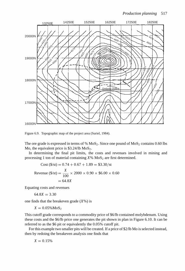
Production planning
18250E17250E16250E15250E14250E13250E
20000N
19000N
18000N
17000N
16000N
445044754500
45254550
45754600
4700
4625
46504675
4750
4775
4800
472546
75
4650
462546
004575
455045
254500
445044
254400
4475
4575
4550 45
25
4500
4475
4450
4425
4400
Orebody Outline
Figure 6.9. Topographic map of the project area (Suriel, 1984).
The ore grade is expressed in terms of % MoS2. Since one pound of MoS2 contains 0.60 lbsMo, the equivalent price is $3.24/lb MoS2.
In determining the final pit limits, the costs and revenues involved in mining andprocessing 1 ton of material containing X% MoS2 are first determined.
Cost ($/st) = 0.74 + 0.67 + 1.89 = $3.30/st
Revenue ($/st) = X
100× 2000 × 0.90 × $6.00 × 0.60
= 64.8X
Equating costs and revenues
64.8X = 3.30
one finds that the breakeven grade (X%) is
X = 0.05%MoS2
This cutoff grade corresponds to a commodity price of $6/lb contained molybdenum. Usingthese costs and the $6/lb price one generates the pit shown in plan in Figure 6.10. It can bereferred to as the $6 pit or equivalently the 0.05% cutoff pit.
For this example two smaller pits will be created. If a price of $2/lb Mo is selected instead,then by redoing the breakeven analysis one finds that
X = 0.15%
517

Open pit mine planning and design: Fundamentals
12750
20000
19000
18000
17000
16000
4450
4750
3550
Cutoff � 0.05% MoS2
Scale 1:1000 JRS
13750 14750 15750 16750 17750
Figure 6.10. Pit outline for a 0.05 cutoff (Suriel, 1984).
The $2 pit is shown in Figure 6.11. For a price of $1.50/lb Mo, the breakeven grade is
X = 0.20%
Figure 6.12 is a plan view of the resulting $1.50 pit. The three nested pits are shown onsection 18000 N in Figure 6.13.
With this approach one would begin (Phase I) with the mining of the 0.20% MoS2 ($1.50)cutoff pit. Phase II involves the material in the 0.15% MoS2 ($2) cutoff pit and finally, PhaseIII, the 0.05% MoS2 ($6) cutoff pit. Pits intermediate to these can be found by selectingthe appropriate price. As can be seen in Figure 6.13, barren material overlies the orebody.All material down to the 4400 level will be stripped and sent to a waste dump. Its removalrequires drilling and blasting. There is also some low grade material running 0–0.05%MoS2below this level. The grade-tonnage distribution for the overall pit is shown in Table6.6. There are 102,970,000 tons above the 0.05% cutoff. The average grade is 0.186%. Thegrade-tonnage distributions for the 3 mining phases are given in Table 6.7.
The average grade of the material above 0.05% for each of the 3 phases is:
Phase I : g = 0.225%
Phase II : g = 0.182%
Phase III : g = 0.176%
An initial decision has been made to mine the orebody over a period of 15 years. Thusthe average milling rate will be of the order of 6.9 × 10⁶ tons/year. Assuming that the milloperates 250 days/year the daily milling rate is 27,500 tpd. In reviewing the level plans,
518

Production planning
12750
20000
19000
18000
17000
16000Scale 1:1000
3850
4450
4750
JRS
Cutoff � 0.15% MoS2
13750 14750 15750 16750 17750
Figure 6.11. Pit outline for a 0.15 cutoff (Suriel, 1984).
12750
20000
19000
18000
17000
16000Scale 1:1000
Cutoff � 0.20% MoS2
JRS
13750 14750 15750
4750
4050
4450
16750 17750
Figure 6.12. Pit outline for a 0.20 cutoff (Suriel, 1984).
519

Open pit mine planning and design: Fundamentals
14000E5000
4000
3000
CROSS-SECTION 18000NSCALE 1:500 JRS
Elevation
15000E
0.20
0.15
0.05
16000E
Figure 6.13. Cross-section 18000 N showing the three pit outlines (Suriel, 1984).
Table 6.6. Mineral inventory for the molybdenum pit.
Grade (% MoS2) Tons (103)
0 (overburden) 86,4100 < g < 0.05 50,720
0.05 ≤ g < 0.10 10,4200.10 ≤ g < 0.15 23,4300.15 ≤ g < 0.20 29,0100.20 ≤ g < 0.25 22,300
g∗ ≥ 0.25 17,810
Total = 240,100
∗The average grade is 0.30%.
Table 6.7. Mineral inventory by phase.
Grade (% MoS2) Tons (103)
Phase I Phase II Phase III
0 (overburden) 36,260 21,440 28,7100 < g < 0.05 680 6170 43,870
0.05 ≤ g < 0.10 180 1640 86000.10 ≤ g < 0.15 1710 9700 12,0200.15 ≤ g < 0.20 4530 11,060 13,4200.20 ≤ g < 0.25 4260 5670 12,370
g∗ ≥ 0.25 5670 4860 7280
∗ The average grade is 0.30%.
520

Production planning
it is seen that 57,700,000 tons of rock overburden (the Phase I and Phase II overburden)must be removed in a pre-production period in order to have 6 months ore supply availableat the time of production. This leaves 182,400,000 tons to be mined (ore and waste) duringthe production period. Assuming that the mine also works 5 days/week, the daily miningrate is
Mining rate = 48,600 tpd
The same equipment fleet will be used for the prestripping as the production mining. Duringthe first year of stripping the average daily production rate will be assumed to be 1
3 thatmaintained in later years due to equipment delivery, personnel training, and limited workingplace. Thus the time required for the prestripping is
t (yrs) = 57,700,000
(48,600(t − 1) + 16,200 × 1)250∼= 5.4 yrs
To complete the stripping in 5 years the actual waste mining rate will be
Year 1 = 18,000 tpd
Years 2 to 5 = 53,200 tpd
With this milling rate, there are approximately 2.4 years of reserves in Phase I and 4.8years of reserves in Phase II. Phase III represents the reserves for years 7.2 through 15. Thefollowing data will be used:
Total material to be mined = 240,100,000 tons
Ore grade > 0.05% MoS2 material = 102,970,000 tons
Average ore grade = 0.186% MoS2
Mill recovery = 90%
Price = $3.24/lb MoS2
Mining rate = 48,600 tpd
Milling rate = 27,500 tpd
Operating time = 250 days per year
Total material to be pre-stripped = 57,700,000 tons
Pre-stripping period = 5 years
Stripping rate year 1 = 16,200 tpd
Stripping rate years 2−5 = 48,600 tpd
This example is continued in the cash flow calculations of Section 6.5.
6.5 CASH FLOW CALCULATIONS
In Section 6.4 the concept of nested pits was discussed with respect to a molybdenum ore-body. In this section the example will be continued with consideration of the resulting cash
521

522 Open pit mine planning and design: Fundamentals
Table 6.8. Assumed schedule for the pre-production period (Suriel, 1984).
Year
1 2 3 4 5 6 7
Exploration � �Property acquisition �Development � � � � �
flows. The basic ideas involved with cash flow calculations were introduced in Chapter 2.The specific application, however, has been left to this section. Each state, province, andcountry has specific rules and regulations regarding taxes, depreciation, depletion, royal-ties, etc. Even for a given state these rules change with time. Therefore, the authors haveselected a somewhat simplified example originally presented by Suriel (1984) to illustratethe calculations involved. Hopefully the reader can adapt the procedures to fit the applica-tion at hand. The example applies roughly to an orebody located in the State of Coloradoin the year 1983. Certain aspects of the laws in effect at the time such as minimum taxand investment tax credit have been left out since they add unnecessary complication to theexample. It has been assumed that the mining company is a division of a profitable cor-poration. Costs involved in the development of this new mine will be expensed wheneverpossible.
In the mine life two periods will be considered:– pre-production period, and– production period.
Today there is generally a third period, the post-production or closure period in whichfinal reclamation takes place. This is not covered here. The pre-production period which isassumed to require 7 years, can be broken down into 3 different and distinct expenditurecategories:
– detailed exploration,– property acquisition, and– infrastructure and mine development.
A representative schedule of activities is illustrated in Table 6.8. The first two years are usedfor detailed exploration work. Property acquisition takes place in year 2. The following5 years are required for infrastructure and mine development. Hence, the pre-productionperiod requires a total of 7 years. Production is expected to take place over a period of15 years.
The basic line items in the pre-production cash flow calculation are given in Table 6.9.A brief discussion of each line item will be presented below. The numerical values for thisexample have been inserted in Table 6.10.
Lines 1 and 2: Project year and Calendar year. The first calendar year in which majorexpenditures occur is 1984. For the cash flow calculations this is selected as project year 1.Discounting will be done back to the beginning of year 1984 (project year 1).
Line 3: Capital expenditures. The ‘capital’ expenditures include a variety of different typesof items ranging from hardware (mine and mill equipment) to royalties and property taxes.They occur at varying times in the cash flow table.
pjw
stk|
4020
64|1
4356
0352
4

Production planning
Table 6.9. Typical pre-production cash flow categories (Suriel, 1984).
1. Project year 1 2 Last year of2. Calendar year 1984 1985. . . pre-production
3. Capital expenditures:
4. Property acquisition5. Royalties6. Exploration7. Development8. Mine and mill buildings9. Mine and mill equipment
10. Property tax11. Working capital
12. Total capital expenditures
13. Cash generated due to tax savings:
14. Exploration15. Development16. Depreciation17. Property tax
18. Total cash generated
19. Net cash flow
Line 4: Property acquisition costs $2,000,000. It takes place in project year 2. This expen-diture is a primary component of the depletion account which controls unit depletionallowance.
Line 5: Royalties. In addition to receiving $2,000,000 for the property, the original ownerswill receive a royalty. Normally these royalties are a certain percentage of the net smelterreturn (NSR). In this case the royalty is 5% of the mill return. No royalty is, therefore, paidduring the pre-production period.
Line 6: Exploration. As defined in the U.S. tax law, exploration costs are those incurred priorto any development of the deposit. Exploration refers to the activities performed in order todetermine the location, size, extent, quality, and quantity of a mineral occurrence. The readeris encouraged to compare this interpretation with that appropriate at the specific location andtime. The U.S. Internal Revenue Service (IRS) allows the firm to choose between two sep-arate methods in accounting for exploration expenditures: capitalize exploration costs intothe depletion account and allocate them over time as production occurs, or treat explorationcosts as annual expenses. For this example, the exploration costs are broken down as follows:
Year 1 = $1,500,000
Year 2 = $1,000,000
To simplify the example, these have been fully expensed in the years in which they occurred.
Line 7: Development. In this example site development consists of three individual lineitems:
(a) Site preparation.(b) Pre-production stripping.(c) Plant site cleaning and mass excavation.
523

524 O
pen pit mine planning and design: F
undamentals
Table 6.10. Pre-production cash flow table ($1,000).
1. Project year 1 2 3 4 5 6 72. Calendar year 1984 1985 1986 1987 1988 1989 1990
3. Capital expenditures: Total4. Property acquisition 0 2000 0 0 0 0 0 20005. Royalties 0 0 0 0 0 0 06. Exploration 1500 1000 0 0 0 0 0 25007. Development 0 0 3330 9842 9842 9842 9842 42,6988. Mine/mill buildings 0 0 0 4836 13,057 1711 9948 29,5529. Mine/mill equipment 0 0 10,000 0 9981 25,295 2999 48,275
10. Property tax 0 0 255 378 965 1654 1985 523711. Working capital 0 0 0 0 0 0 8353 8353
12. Total capital expenditures 1500 3000 13,585 15,005 33,744 38,349 33,127 138,310
13. Cash generated due to tax savings14. Exploration 690 460 0 0 0 0 0 115015. Development 0 0 1532 4527 4527 4527 4527 19,64016. Depreciation 0 0 0 920 920 920 920 368017. Property tax 0 0 117 150 397 690 819 2173
18. Total cash generated 690 460 1649 5597 5844 6137 6266 26,643
19. Net cash flow −810 −2540 −11,936 −9408 −27,900 −32,212 −26,861 −111,667
pjw
stk|
4020
64|1
4356
0353
0

Production planning 525
General site preparation (cost = $1,729,000) as well as the plant site cleaning (cost =$859,000) will occur in project year 3. The total amount of pre-production stripping is57,700,000 tons. Since the expected cost per ton is $0.74, the total cost is $42,698,000.The stripping schedule is as follows:
Project year Amount stripped (tons) Cost ($)
3 4,500,000 (18,000 tpd) 3,330,0004 13,300,000 (53,200 tpd) 9,842,0005 13,300,000 9,842,0006 13,300,000 9,842,0007 13,300,000 9,842,000
These costs are expensed in the year incurred.
Line 8: Mine and mill buildings. There are 7 items which fall into this category. Theyare indicated below together with their cost and the project year in which the expenditureis made.
Item Project year Cost ($)
1. Concrete foundation and detailed excavation 4 $4,836,0002. Open-pit maintenance facilities 7 $6,623,0003. Concentrator building 5 $13,057,0004. Concentrate storage and loading 7 $139,0005. Capital cost of general plant service 6 $1,711,0006. Tailings storage 7 $1,775,0007. Water supply 7 $1,411,000
These items, considered as improvements to the property, will be depreciated (straight line)over a 20 year period beginning in production year 1. Capital gains and losses will beignored.
Line 9: Mine and mill equipment. There are 6 items which fall into this category. Theyare indicated below together with their cost and the project year in which the expenditureis made.
Item Project year Cost ($)1. Open-pit equipment 3 $10,000,0002. Crushing plant, coarse ore storage and conveyors 5 $9,981,0003. Grinding section and fine ore storage 6 $16,535,0004. Flotation section 6 $6,985,0005. Thickening and filtering 6 $1,775,0006. Electric power supply and distribution 7 $2,999,000
The open-pit equipment is broken down as follows:
(a) Shovels (3-15 yd3) = $3,000,000(b) Trucks (12-150 ton) = $5,000,000(c) Drills, graders, dozers = $2,000,000

526 Open pit mine planning and design: Fundamentals
The equipment in categories (b) and (c) will be replaced every 5 years. Since this fleet willbe used for the stripping as well as the production mining, there will be a capital expenseof $7,000,000 in project years 1, 6 and 11. The shovels are expected to last the life of themine. Straight line depreciation over a period of 5 years is used. There is no salvage. Theequipment will be put into use in the year purchased, hence, depreciation will begin then.
Items 2 through 6 will be depreciated over a 7 year period (straight line, no salvage)beginning in production year 1.
Line 10: Property tax. This tax, sometimes called ad valorem tax is one of the most commontypes of state tax. Property tax in Colorado is assessed on: (a) personal and real propertyand (b) ore sales.
Colorado taxes personal and real property at 30% of the actual value of the property. Inthis case personal property is that listed in line 9 and real property in line 8. The taxablevalue for real and personal property is determined by its base year value. The tax is thendetermined by multiplying the total assessed value by a rate called the ‘pro mille’ levy or inthe U.S. simply the ‘mill’ levy. In Colorado the ‘pro mille’ levy varies from county to county.In this case study that used is 85 (corresponding to that applied by Jefferson County). Thismeans that the appropriate factor is 85/1000 or 0.085. The assessed value for the calculationof the property tax on ore sales is: (a) 25 percent of gross proceeds or (b) 100 percent of netproceeds, whichever is greater.
Gross proceeds are defined as the gross value of the ore produced minus treatment,reduction, transportation and sales cost at the mine mouth. Net proceeds is equal to thegross proceeds minus all costs associated with extraction of the ore. In Colorado, royaltiesare not deductible for either case. The pro mille levy is applied to the assessed value.
Line 11: Working capital. This represents the amount of money necessary to cover operatingcosts during a portion of the project’s life. Working capital consists of cash, inventories(parts, supplies and concentrate) and accounts receivable. Working capital was estimated atfour months of operating costs. It was allocated to the last year of the pre-production periodbefore production start up (project year 7). The account is maintained during the productionperiod and recovered at the end of project life. In this case, the amount of required workingcapital is $12,383,000.
Line 12: Total capital expenditures. This is the sum year by year of line items 4 through 11.
Line 13: Cash generated due to tax savings. As indicated earlier, the mining company isone division of a large profitable corporation. The corporate structure enables the companyto expense most costs whenever possible and generate tax savings during the preproductionperiod. The federal tax rate is 46 percent.
To illustrate this assume that the corporation has an income subject to federal tax, prior toincluding this mining venture, of $10,000,000. At a tax rate of 46%, the corporation wouldpay $4,600,000 in federal tax. However, in project year 1, the mining division incurs anexploration expense of $1,500,000. If this is considered as an expense of the corporation,then the taxable income of the corporation would drop from $10,000,000 to $8,500,000.The tax on this amount is $3,910,000. Hence, there is a tax savings of $690,000 for the cor-poration. This has been included on the cash flow table for the mining company (Table 6.10)under ‘Cash generated due to tax savings – Exploration’. Similar ‘tax savings’ occur withregard to development, depreciation and property tax when they are applied against otherincome.

Production planning 527
Line 14: Exploration. The exploration expenses result in a tax savings of $690,000 (0.46 ×$1,500,000) in project year 1 and $460,000 in project year 2.
Line 15: Development. Stripping, site preparation, etc., costs are multiplied by the tax rateand included here.
Line 16: Depreciation. Straight line depreciation of the mining equipment begins in projectyear 3. The yearly amount is multiplied by the tax rate.
Line 17: Property tax. The property tax is the assessed value multiplied by the tax rate.
Line 18:Total cash generated. The items in lines 14 through 17 are summed and entered here.
Line 19: Net cash flow. The total capital expenditures (line 12) are subtracted from the totalcash generated (line 18). This is the net cash flow.
The basic line items in the production period cash flow calculation are given in Table 6.11.A brief discussion of these will be presented below.
Line 1, 2, and 3: Production, project and calendar year. The first year of production is1991 which is the eighth year of the project. In doing the discounted cash flows and NPVcalculations, they will be brought back to the beginning of the project.
Line 4: Revenue. Revenue is calculated by multiplying concentrate tonnage by the price ofmolybdenite concentrate at the mill site. The molybdenite concentrate price is estimated
Table 6.11. Typical production period cash flow categories (Suriel, 1984).
1. Production year2. Project year3. Calendar year
4. Revenue5. Royalty
6. Net revenue7. Mining cost8. Processing cost9. General cost
10. Property tax11. Severance tax12. Depreciation13. State income tax
14. Net income after costs15. Depletion
16. Taxable income17. Federal income tax
18. Profit19. Depreciation20. Depletion
21. Cash flow
22. Capital expenditures23. Working capital
24. Net cash flow

528 Open pit mine planning and design: Fundamentals
at $6 per pound of contained molybdenum. Concentrate tonnage is equal to ore tonnagemultiplied by average grade, the mill recovery, and by the concentrate percent of Mo.(MoS2 contains about 60% Mo.)
Line 5: Royalty. The royalty is 5 percent of the revenue.
Line 6: Net revenue. This is the difference between revenue and the royalty payment.
Line 7: Mining cost. The mining cost depends somewhat on the production rate as can beseen in Figure 6.14 and in Table 6.12. Because 57,700,000 tons have been mined in thepre-production period, 182,400,000 tons remain. The length of the production period hasbeen selected as 15 years, and the mine will work 5 days per week (250 days per year). Thusthe mining rate is 48,640 tons per day. From Figure 6.14, the mining cost of $0.77/ton hasbeen selected.
Line 8: Processing cost. The mill will also run 5 days per week, 250 days per year.The mill cutoff grade has been selected as 0.05% MoS2 hence there are 102,970,000tons to be processed. The milling rate is therefore 27,460 tons/day and yearly ore pro-duction is 6,865,000 tons. The milling cost selected from Figure 6.15 and Table 6.12 is$1.93/ton.
Line 9: General and administrative cost. This cost has been computed per ton of ore pro-cessed. Its value as can be seen in Figure 6.16 and Table 6.12 is $0.67/ton. In some operationsthere is a G&A cost attached to waste removal as well. This has not been done here.
Line 10: Property tax. The property tax is computed in the same way as was discussed forthe pre-production period. The assessed value is 30% of the initial cost and the pro mille rateis 85 (0.085). The value at the end of the pre-production period is $77,827,000. Applyingthe 30% assessed valuation and the 85 pro mille levy, the annual property tax is $1,985,000.
00
0.50
1.00
Min
ing
Cos
t ($/
Ton)
1.50
2.00
10000 20000 30000
Mining Capacity (Tons/Day)
40000 50000 60000
Figure 6.14. Mining cost versus mining capacity (Suriel, 1984).

Production planning 529
This annual value will be carried throughout the production period. The book value has notbeen used and the effect of replacement capital has not been included.
The gross revenue from annual ore sales is $82,742,000. The net revenue after sub-tracting mining, processing, and general costs is $57,683,000. Note that royalties have not
5.00
4.00
3.00
2.00
1.00
00 10000 20000 30000
Milling Capacity (Tons/Day)
40000
Mill
ing
Cos
t ($/
Ton)
Figure 6.15. Milling cost versus milling capacity (Suriel, 1984).
2.00
1.50
1.00
Adm
inis
trat
ive
Cos
t ($/
Ton)
0.50
00 10000 20000 30000 40000
Milling Capacity (Tons/Day)
Figure 6.16. Administrative cost versus milling capacity (Suriel, 1984).

530 Open pit mine planning and design: Fundamentals
been subtracted. Applying the two rules (25 percent of gross proceeds or 100 percent ofnet proceeds) one finds that the greatest amount (which becomes the assessed valuation)is $57,683,000. Applying the 85 pro mille levy, this contribution to the property tax is$4,903,055. Thus the total annual property tax is $6,888,055.
Line 11: Severance tax. A severance tax is levied for removing or ‘severing’the mineral fromthe earth and the state/country. Colorado imposes a such severance tax on molybdenum. Itwas imposed on production at a rate of $0.15 per ton of ore.
Line 12: Depreciation. The depreciation allowance is a deduction over a period of yearsfor use, deterioration, wear and tear of depreciable assets used in generating income forthe project. Depreciable assets for a mining project are grouped into either personal orreal property. Mine and mill equipment are considered personal property. The total valueis $48,275,000. The open pit mining equipment is depreciated over 5 years. The initialinvestment is $10,000,000 in project year 3 while replacement equipment (trucks, drills,etc.) at a cost of $7,000,000 is purchased in project years 8, 13, and 18. The remainderof the mine and mill equipment (initial cost of $38,275,000) is depreciated over a sevenyear period beginning at the start of production. Real property, including mine and millbuildings and improvements, amount to $29,552,000. A twenty year life is used for realproperty with depreciation beginning at the start of production. Thus the depreciation peryear is $1,477,600. The depreciation by class and year is shown in Table 6.13.
Line 13: State income tax. The state tax is 5% of the net income. In computing the netincome the following deductions are allowed:
– royalties,– operating costs,– depreciation,– property tax,– severance tax, and– depreciation.
For production years 1 through 7 the state income tax is $1,864,000. For years 8 through15 it is $2,138,000.
Line 14: Net income after costs. This is the net revenue (line 6) minus lines 7 through 13.
Line 15: Depletion. In order to recognize that minerals, oil, and gas are non-renewable assetswhich are depleted through production, the U.S. government permits a depletion allowanceto be deducted prior to the calculation of federal taxable income. For mineral resources thedepletion allowance is calculated and claimed by either of two methods, whichever givesthe largest amount of pre-tax deduction. It is permissible to change methods from year toyear. The two methods for calculating the depletion allowance are statutory depletion andcost depletion.
For statutory depletion, the amount which can be deducted is the smaller of: (a) 50 percentof net income or (b) a certain percentage of net revenue (revenue minus royalties). For the(a) calculation, net income is defined as revenues minus royalties, operating costs, statetaxes, and depreciation. For (b) the percentage depletion for molybdenum is 22 percent.Note that the amount of depreciation varies throughout the life of the mine. For the first 7years of production it is $8,346,000 per year. The annual net income during this period is$35,418,000 and hence, the allowable depletion on this basis is $17,709,000.

Production planning
531
Table 6.12. Assumed operating cost data (Suriel, 1984).
Cutoff Geologic 90% Average Tonnage Tonnage Total Total General & Totalgrade reserves geologic grade milled mined mining milling administrative operating% MoS2 (× 106 st) reserves % M0S2 (tpd) (tpd) cost cost cost cost
(× 106 st) ($/ton) ($/ton) ($/ton) ($/ton)
0.30 12.680 11.412 0.40 2173 3043 1.91 4.64 1.93 8.480.25 24.390 21.950 0.34 4181 5854 1.65 3.55 1.39 6.350.20 51.300 46.170 0.28 8794 12,312 1.33 2.65 0.97 4.950.15 107.010 96.309 0.22 18,345 25,682 1.00 1.98 0.68 3.660.10 181.490 163.341 0.18 31,113 43,558 0.80 1.91 0.67 3.380.05 228.280 205.452 0.16 39,134 54,787 0.74 1.89 0.67 3.30
Table 6.13. Depreciation by class and project year.
Depreciation Project year depreciation ($1000)class (yrs)
1 2 3 4 5 6 7 8 9 10 11 12 13 14 15 16 17 18 19 20 21 22
5 0 0 2000 2000 2000 2000 2000 1400 1400 1400 1400 1400 1400 1400 1400 1400 1400 1400 1400 1400 1400 14007 0 0 0 0 0 0 0 5468 5468 5468 5468 5468 5468 5468 0 0 0 0 0 0 0 0
20 0 0 0 0 0 0 0 1478 1478 1478 1478 1478 1478 1478 1478 1478 1478 1478 1478 1478 1478 1478
Total 0 0 2000 2000 2000 2000 2000 8346 8346 8346 8346 8346 8346 8346 2878 2878 2878 2878 2878 2878 2878 2878

532 Open pit mine planning and design: Fundamentals
The annual net revenue is $78,605,000. Taking 22% of this number yields $17,293,000.The lesser of these two numbers is $17,293,000.
Cost depletion is based on the cost of the property, non-expensed exploration costs,number of units of mineral sold during the year and reserves available in the deposit at theend of the year. Cost depletion is calculated by multiplying the adjusted basis, (equivalentto all property acquisition costs plus capitalized exploration costs) by the tons mined duringthe year divided by remaining reserves. The adjusted basis is reduced each year by thedepletion allowance claimed.
Cost depletion = (Adjusted basis) × Mineral units removed during the year
Mineral units recoverable at start of the year
Adjusted basis = Cost basis ± Adjustments
−Cumulative depletion allowance claimed
In this case the cost of the property was $2,000,000. For the first year, 6,865,000 tons ofore are mined. The initial ore tonnage is 102,970,000. Hence, for year 1 the allowable costdepletion would be
$2,000,000 × 6,865,000
102,970,000× $133,340
The greater of the cost and percentage depletion values is chosen. Thus, one chooses$17,293,000 to be deducted. However, according to the tax rules one must recapture theexploration expense of $2,500,000 by reducing the amount of depletion earned. Hence, inyear 1, the allowed depletion deduction is $17,293,000 − $2,500,000 = $14,793,000.
In year 2 the statutory depletion allowance is $17,293,000. For the cost depletioncalculation the adjusted basis is
Adjusted basis = Cost basis − Cumulative depletion
The cost basis is $2,000,000. The cumulative depletion already taken (through project year8) is $14,793,000. Hence the adjusted basis is
Adjusted basis = $2,000,000 − $14,793,000 = −$12,793,000
The cost of the property was fully recovered through depletion in production year 1 andhence only statutory depletion is used for the remaining mine life. In production year 2, afull depletion of $17,293,000 is taken since all previously expensed exploration costs havebeen recaptured.
Line 16: Taxable income. This is the net income after cost (line 14) minus depletion (line 15).
Line 17: Federal income tax. In this case the federal income tax is 46% of the taxableincome.
Line 18: Profit. The profit is the taxable income minus the federal income tax.
Line 19 and 20: Depreciation and depletion. These two items which had been previouslyconsidered as expenses when computing taxes are now added to the profit to arrive at acash flow.
Line 21: Cash flow. This is the sum of lines 18 through 20.
Line 22: Capital expenditures. In years 1, 6, and 11 new trucks, drills, dozers, etc., arepurchased. The capital cost involved in each of these years is $7,000,000.

Production planning 533
Line 23: Working capital. The working capital was allocated to the last year of thepre-production period before production start-up. The account is maintained during theproduction period and recovered at the end of project lift (project year 22).
Line 24: Net cash flow. The net cash flow for any particular year is the sum of lines 21, 22,and 23.
The cash flows during the production period are summarized in Table 6.14.
6.6 MINE AND MILL PLANT SIZING
6.6.1 Ore reserves supporting the plant size decision
In the preceding sections, the final pit limits have been determined using the following steps:1. The metal content of a block together with forecasted sales prices and estimated full
scale plant metallurgical recoveries are used for determining the revenue.2. Production costs through to sales and shipping costs are estimated.3. A net value is calculated for each block. A block with a net value equal to zero is one
where the revenues equal the production costs. The grade corresponds to a mining cutoff.4. A computer technique (such as the floating cone) is used to identify all blocks capable
of paying for the costs of uncovering them. These are included within the final pit.5. A mineral inventory – ore reserve is constructed.6. Milling and mining rates are assumed and the associated capital costs determined. For
example a series of different milling cutoff grades might be applied to the total pool ofmaterial. Mill ore quantities would be calculated. These reserves would be used to size themill plant.
7. A financial analysis would be conducted for each alternative to determine the NPV,internal ROR, etc. The best option would be selected.
As can be seen, the introduction of the capital cost takes place at a very late stage. Theprofit is an output rather than an input. After having gone through this entire process, it maybe that the rate of return is too low. The process would then have to be repeated focussingon the higher grade ore, using a different (lower) production rate, reducing the investmentin mine and mill plant, etc. In the process just described a variety of materials of differenteconomic value are being mined at any one time. Those with the highest values contributemore to paying off the investment and profit than those of lower value. The summing orintegration of these values occurs for a given production year. This overall value is used asan entry in the cash flow table. To illustrate this concept, assume that there are 60 ore blocksto be mined in a given period. The net value distribution (at step 3, prior to introducing thecapital cost and profit) is as follows:
Grade Net value/block No. of blocks Net value
g1 $0 10 $0g2 $10 10 $100g3 $20 10 $200g4 $30 10 $300g5 $40 10 $400g6 $50 10 $500

534 O
pen pit mine planning and design: F
undamentals
Table 6.14. Cash flow during mine production life ($1000).
1. Production year 1 2 3 4 5 6 7 8 9 10 11 12 13 14 152. Project year 8 9 10 11 12 13 14 15 16 17 18 19 20 21 223. Calendar year 1991 1992 1993 1994 1995 1996 1997 1998 1999 2000 2001 2002 2003 2004 2005 Total
4. Revenue 82,742 82,742 82,742 82,742 82,742 82,742 82,742 82,742 82,742 82,742 82,742 82,742 82,742 82,742 82,742 1,241,1305. Royalty 4137 4137 4137 4137 4137 4137 4137 4137 4137 4137 4137 4137 4137 4137 4137 62,055
6. Net revenue 78,605 78,605 78,605 78,605 78,605 78,605 78,605 78,605 78,605 78,605 78,605 78,605 78,605 78,605 78,605 1,179,0757. Mining cost 9363 9363 9363 9363 9363 9363 9363 9363 9363 9363 9363 9363 9363 9363 9363 140,4458. Processing cost 13,249 13,249 13,249 13,249 13,249 13,249 13,249 13,249 13,249 13,249 13,249 13,249 13,249 13,249 13,249 198,7359. General cost 4600 4600 4600 4600 4600 4600 4600 4600 4600 4600 4600 4600 4600 4600 4600 69,000
10. Property tax 6888 6888 6888 6888 6888 6888 6888 6888 6888 6888 6888 6888 6888 6888 6888 103,32011. Severance tax 1030 1030 1030 1030 1030 1030 1030 1030 1030 1030 1030 1030 1030 1030 1030 15,45012. Depreciation 8346 8346 8346 8346 8346 8346 8346 2878 2878 2878 2878 2878 2878 2878 2878 81,44613. State income tax 1756 1756 1756 1756 1756 1756 1756 2030 2030 2030 2030 2030 2030 2030 2030 28,532
14. Net income after costs 33,373 33,373 33,373 33,373 33,373 33,373 33,373 38,567 38,567 38,567 38,567 38,567 38,567 38,567 38,567 542,14715. Depletion 14,793 17,293 17,293 17,293 17,293 17,293 17,293 17,293 17,293 17,293 17,293 17,293 17,293 17,293 17,293 256,895
16. Taxable income 18,580 16,080 16,080 16,080 16,080 16,080 16,080 21,274 21,274 21,274 21,274 21,274 21,274 21,274 21,274 285,25217. Federal income tax 8547 7397 7397 7397 7397 7397 7397 9786 9786 9786 9786 9786 9786 9786 9786 131,217
18. Profit 10,033 8683 8683 8683 8683 8683 8683 11,488 11,488 11,488 11,488 11,488 11,488 11,488 11,488 154,03519. Depreciation 8346 8346 8346 8346 8346 8346 8346 2878 2878 2878 2878 2878 2878 2878 2878 81,44620. Depletion 14,793 17,293 17,293 17,293 17,293 17,293 17,293 17,293 17,293 17,293 17,293 17,293 17,293 17,293 17,293 256,895
21. Cash flow 33,172 34,322 34,322 34,322 34,322 34,322 34,322 31,659 31,659 31,659 31,659 31,659 31,659 31,659 31,659 492,37622. Capital expenditures 7000 0 0 0 0 7000 0 0 0 0 7000 0 0 0 0 21,000
23. Working capital 0 0 0 0 0 0 0 0 0 0 0 0 0 0 8353 8353
24. Net cash flow 26,172 34,322 34,322 34,322 34,322 27,322 34,322 31,659 31,659 31,659 24,659 31,659 31,659 31,659 23,306 463,023

Production planning 535
There are 50 associated waste blocks each carrying a value of −$20. Thus the apparent totalnet value for this period would be $500. At first glance this might appear good. Howeverwhen a cash flow calculation (now including the capital cost and profit) is made, it is foundthat the desired rate of return is too low. The required net value at step 3 is $1,100 ratherthan $500. Since there are 60 ore blocks involved, this would mean an average ‘assessment’of $10/block. If this is done then the modified net value distribution becomes
Grade Net value/block No. of blocks Net value
g1 −$10 10 −$100g2 $0 10 $0g3 $10 10 $100g4 $20 10 $200g5 $30 10 $300g6 $40 10 $400
Clearly those blocks with grade g1 are not contributing their fair share of the capital invest-ment and profit. Thus the cutoff grade should be g2 rather than g1. The number of ore blockswould drop from 60 to 50. If the plant size is not changed, this translates into a shorterproperty life which changes the cash flow which in turn would affect the $10 average blockassessment. If the mine life is maintained constant, then the size of the mill plant should bereduced. This also affects the cash flow. For this situation, perhaps the average assessmentper block would drop to $5/block. The number of blocks would increase again and theprocess would be repeated.
One way of handling this problem early on is to include a cost item for capital and profitamongst those used to generate the economic block model. These costs would then becovered up front.
The alternative sequence of steps is listed below (Halls et al., 1969):1. The metal content of a block, together with forecasted sales prices and estimated
full-scale plant metallurgical recoveries is used for determining the revenue.2. Production costs through to sales and shipping costs are estimated.3. The amount of depreciation to be added to the operating costs is calculated on a
straight line basis by dividing the estimated capital expenditure by the estimated ore reservetonnage.
4. A minimum profit after tax, related to minimum acceptable return on investment isassigned to each block.
5. The net value for each block is calculated. The ‘cutoff grade’ used to separate orefrom waste is that grade of material which produces a revenue equal to the production coststhrough to sales together with depreciation and minimum profit.
6. Using the above data the computer will include all blocks of material in the ore reservewhich are capable of producing more than the minimum pre-determined profit (after taxes)after paying for the stripping costs necessary to uncover them.
There are no real difficulties in assessing the revenues to be produced from a block or theproduction costs involved in producing its metal for sale, including such considerations ascost variations due to varying haulage distances and rock types. It is, however, extremelydifficult to estimate unit depreciation and required minimum profit per ton accurately beforethe ore reserve tonnage is known because both
– depreciation, and– required minimum profit

536 Open pit mine planning and design: Fundamentals
Mining Period 1
Mining Period 2
Mining Period 3
Revenue Covers Costs, Depreciationand Provides a Return on
Investment
Revenue Covers Costs and Depreciation
Revenue Covers Costs but Does Not FullyCover Depreciation,
The Deliberate Construction of Plantfor This Ore Cannot Be Justified.
The Ore is Worth Processing in anEssentially Fully Depreciated Plant
Pit Limit Increment RevenueCovers Costs Only. Does Not
Provide a ContributionTowards Depreciation.
Figure 6.17. Economic pit limits as a function of included costs (Halls et al., 1970).
will vary with plant size and total ore tonnage. In order to estimate depreciation and profit– an ore reserve tonnage,– a production rate, and– an effective tax rate
must be assumed. An iteration process is used until convergence between the assumed andfinal values is achieved.
The resulting pit is shown as the ‘Mining Period 1’ pit in Figure 6.17. A second pitoutline can be produced by eliminating the required profit (profcost) assessed each block.The depreciation cost would remain, however. By eliminating the profit cost element andkeeping the other costs and revenues the same, the positive block values would increase.Each positive block would be able to carry more stripping and the pit would increase insize. This is shown by the ‘Mining Period 2’ pit. The ‘no-profit’ condition only applieswhen determining the pit limit. The average ore grade of the material between the MiningPeriod 1 and 2 limits would be higher than the pit limit cutoff. Hence a profit is realized. Toincrease the size of the pit further, the depreciation cost would have to be dropped from theeconomic block model calculation. This further lowers the grade required to produce positivevalued blocks. The pit expands to the limit shown by the heavy shaded line (Mining Period3 limit). As indicated by Halls (1970), plant capacity cannot be deliberately constructedfor this ore. The ore however is worth processing in an essentially fully depreciated plant.Even though a specific profit cost has not been attached to each block in Mining Period 3,there will still be an overall profit since the average ore grade in the period is higher thanthe cutoff. The Mining Period 2 pit encloses those reserves which should be consideredwhen sizing the plant. The final pit outline would be the same as produced by the firstprocedure described in this section. Here however the reserves contained within specificmineable pits are used rather than a certain portion of the overall reserves. There are anumber of objections (Halls, 1970) which have been raised concerning the requirementthat each ore block irrespective of grade contribute an equal portion to profits and capitalpayback:
(a) The only practical way of determining unit depreciation for use in individual blockevaluation is the straight-line method. In the financial evaluation of the ore reserve, the

Production planning 537
depreciation method employed will be the one which reduces the impact of taxation to aminimum. Also it is virtually impossible to incorporate in the cutoff calculations the unitdepreciation which would apply to replacement capital needed throughout the life of themine.
(b) The use of a minimum after-tax profit for each block does not ensure that the summationof the profits from each block will meet the corporate investment goal (except possiblyin the case of an ideal mine, where the annual cash flows remain the same throughoutits life).
(c) In the case of properties which can commence mining in a high-grade portion of thepit, or where taxation benefits are allowed in the initial stages of production, the accurateestablishment of a profit factor to ensure that such increment of investment yields at least aminimum corporate return is an impossibility.
An alternative procedure based upon incremental financial analysis will now be discussed.
6.6.2 Incremental financial analysis principles
The incremental financial analysis approach described in this section is based upon materialoriginally presented by Halls et al. (1969). The rate of return on the total investment isimportant for assessing the potential of a property as a whole. It does not however indicatethe profitability of each capital increment. Only by considering a series of potential pitexpansions and evaluating the yields and returns from each is it possible to ascertain thatevery increment of capital can pay its way. This evaluation process is termed incrementalfinancial analysis. For a new property, the financial returns of alternative ore inventoriesand associated plant sizes for a given mine life (for example) are compared. One beginsfrom the smallest tonnage ore inventory and plant size. Each progressively larger tonnageore inventory is considered as a possible expansion. The additional cash flow developedfrom each expansion is determined as a rate of return on the additional (incremental) cap-ital required for such an expansion. The largest tonnage and hence the lowest grade oreinventory in which every increment of invested capital yields at least the minimum desiredcorporate return is the optimum ore reserve for the assumed life. The process is repeatedusing other realistic lives for the property. These studies provide one basis for the selectionof a depreciation life (depreciation) for the property. As discussed earlier, the actual minelife may be longer than this since once the invested capital has been fully depreciated, thecutoff grade drops (and the reserves increase). This method of optimizing ore reserves andplant size for a new property involves three steps:
Step 1. Calculate ore inventories using arbitrary cutoff grades.Step 2. Prepare a financial analysis for each ore inventory.Step 3. Select that ore inventory which is the optimum ore reserve by incremental financial
analysis.Each of these steps is outlined below.In step 1, a series of arbitrarily chosen, but reasonable, cutoff grades are chosen. For an
open pit copper mine cutoff grades in the range 0.3 to 0.7 percent equivalent copper might bechosen. Using the expected production costs and recoveries, the price needed for breakevenwith the selected cutoff (0.7, for example) would be calculated. Note that no capital costsand profit is included in these calculations. The price together with the costs are then usedto obtain an economic block model. A technique to provide a pit, such as the floating cone,
pjw
stk|
4020
64|1
4356
0353
6

538 Open pit mine planning and design: Fundamentals
00
100
200
300
Mill
Ton
nage
(10
6 to
ns)
400
0.1 0.2 0.3
Mill TonnageAverage M
ill Grade
Mill Cutoff Grade (% Copper)
0.4 0.5 0.6 0.70.4
0.6
0.8
1.0
Ave
rage
Mill
Gra
de (
% C
oppe
r)1.2
1.4
Figure 6.18. Pit material inventory for a 0.7 cutoff grade pit.
Table 6.15. Mill tonnage and average grade as a function of mill cutoffgrade.
Mill cutoff grade Mill tons Avg. grade(% Cu) (× 106 st) (% Cu)
0.70 72 1.290.60 88 1.170.50 116 1.020.40 148 0.900.30 188 0.780 400 0.52
is applied. This would be the 0.7% cutoff grade pit. The inventory of material containedwould be created. One such example is shown in Figure 6.18.
The total tonnage contained is
T = 400 × 106 tons
and the average grade is
g = 0.52% Cu
If the mill cutoff were 0% Cu then this entire amount would be processed. For various millcutoff grades, the total tons and grades are as given in Table 6.15.
All material has to be removed from the pit and the costs of depositing it on surface,whether waste or ore are virtually the same. Therefore some material which is below themining cutoff grade, but within the confines of the pit may be processed at a profit.
Another mining cutoff grade would now be selected, for example 0.6%. The breakevenprice would be calculated and the floating cone run on the deposit again using this price.

Production planning 539
0.70
0.50
0.300.
400.60
Figure 6.19. Pit outlines corresponding to different mining cutoff grades.
A table similar to Table 6.15 would be constructed for this condition. An idealized crosssection showing the series of pits which might be produced is shown in Figure 6.19.
In step 2 a financial evaluation of each ore inventory is prepared. To do this the tonnage andgrade to be mined from the inventory each year must be decided. Lane (1964) has discussedone way of doing this. His approach will be the topic of Section 6.7. Here the same life,25 years, will be used to evaluate all inventories. In practice several realistic lives might betried. Furthermore the production rate will be held constant. Obviously other variations canbe applied. The following data are required to complete the financial evaluations:
(1) the estimated capital costs, broken down into the years in which the money will bespent (including replacement capital),
(2) the estimated operating costs for each production rate,(3) the metal recoveries, based on metallurgical laboratory testing after discounting for
commercial operating conditions,(4) the long- and short-term estimates of metal sales prices,(5) the legally applicable depletion and depreciation allowances which will minimize
taxation, and(6) the current and forecasted taxation rates.
The cash flows for each ore inventory are calculated on a year-by-year basis. Any one of anumber of financial techniques which consider the time value of money can be utilized indetermining the rates of return for both total investment and incremental investment. Thediscounted cash flow (DCF) method will be used here.
In step 3, the different pit expansions are compared. To illustrate the process, considerthe pit generated with the 0.7% Cu cutoff. Two mill cutoffs are considered: 0.7% and 0.6%.The capital investments for mine and concentrator are:
Mill cutoff Capital cost0.7 $43,500,0000.6 $46,832,000
The incremental capital cost is $3,332,000. The annual cash flow for each after taxes is:
Mill cutoff Annual cash flow0.7 $7,550,0000.6 $8,323,000

540 Open pit mine planning and design: Fundamentals
The incremental annual cash flow is $773,000. These cash flows occur over a period of 25years. The net present value of these incremental cash flows is given by
NPVCF = $773,000
[(1 + i)25 − 1
i(1 + i)25
]
where i is the interest rate.These are achieved through the incremental capital investment of $3,332,000.
NPVCI = −$3,332,000
The interest rate (i) which makes the sum of these equal to zero is called the rate of return.In this case
−3,332,000 + 773,000
[(1 + i)25 − 1
i(1 + i)25
]= 0
i = 0.231
Thus there is a 23.1% effective rate of return (ROR) on the incremental investment. Sincethis exceeds the company’s desired rate of 12%, the mill cutoff grade of 0.6% would becomethat used in future comparisons (0.5%, 0.4%, etc.) for the given mining cutoff (0.7%). Thisprocess would continue until ROR values are less than the base.
6.6.3 Plant sizing example
The incremental financial analysis process described in the previous section will now bedemonstrated step-by-step using an example adapted from Halls et al. (1969).
1. Prices and costs are estimated. These are entered into the computer for a floating coneanalysis or are used to generate a stripping ratio – grade curve for a hand analysis.
This is a breakeven analysis such that
Revenue = Costs
The revenue is calculated by
Revenue ($/ton) = 2000 lbs/st
×Recovery (%)
100× Grade (%)
100× Price($/lb) (6.3)
The costs are given by
Costs ($/ton) = Mining ($/st) + Milling ($/st) + G&A ($/st)
+2000 lbs/st × Recovery (%)
100× Grade (%)
100× SRS ($/lb) (6.4)
where SRS is refining, smelting, selling cost ($/lb).Setting Equation (6.3) equal to (6.4) yields
Mining ($/ton) + Milling ($/ton) + G&A ($/ton)
= (Price − SRS) × 2000 lbs
st× Recovery (%)
100× Grade (%)
100(6.5)

Production planning 541
Solving for the cutoff grade one finds that
Grade (%) = [Mining ($/st) + Milling ($/st) + G&A ($/st)]104
[Price ($/lb) − SRS ($/lb)]2000 × Recovery (%)(6.6)
If the expected price is used then the maximum (ultimate) pit will result.
2. The grades and tonnage in the pit are determined. This becomes the reserve of materialto be mined.
Assume the following values:
Mining cost = $0.45/stMilling + G&A = $1.25/stPrice = $0.40/lbSRS = $0.059/lbRecovery = 80%
(Note that for simplicity the G&A has been applied only to the mill (i.e. the ore).)Then the mining cutoff grade becomes
Grade (%) = 0.31%
One would generate a pit with this as the cutoff.Table 6.16 shows that for a pit based upon a 0.3% Cu pit limit cutoff, the tonnage would
be 1,410,000,000. The average grade would be 0.31% Cu (all material). If the mill cutoffgrade were 0% then the entire amount would be sent to the mill. If only those blocks havinga grade of +0.3% were sent to the mill, then the mill tonnage would be 390,000,000 havingan average grade of 0.73% Cu. This would be the largest pit.
3. One could consider smaller pits as well since the biggest pit would not necessarily leadto the desired financial result. This result could be measured in NPV, total profit, returnon investment, etc. Other pits can be generated corresponding to different pit limit cutoffgrades. As can be seen from Equation (6.6), this is a simple matter of just changing theprice. For a lower price, the cutoff grade must go up. In Table 6.16 the following resultswere obtained.
Pit limit Total tons Avg. gradecutoff grade in pit (% Cu)(% Cu) (× 106 st)
0.3 1410 0.310.4 1206 0.330.5 875 0.360.6 650 0.380.7 400 0.40
For each of these ultimate pits all the material would be mined. One must decide whether itshould go to the dump or to the mill.
4. Each of the potential pits is examined with respect to mill and dump material. Considerthe pit developed assuming a final pit cutoff grade of 0.7%. The mill cutoff could be set at

542 Open pit mine planning and design: Fundamentals
Table 6.16. Summary of ore inventory for each mining plan (Halls et al., 1969).
Milling Pit limit cutoff gradecutoff grade
0.7% Cu 0.6% Cu 0.5% Cu 0.4% Cu 0.3% Cu
0.7% Cu Accum. tons 80,000,000Average grade 1.20% CuStripping ratio 4.00 : 1
0.6% Cu Accum. tons 92,000,000 135,000,000Average grade 1.13% Cu 1.12% CuStripping ratio 3.35 : 1 3.81 : 1
0.5% Cu Accum. tons 105,000,000 160,000,000 195,000,000Average grade 1.06% Cu 1.03% Cu 0.99% CuStripping ratio 2.81 : 1 3.06 : 1 3.49 : 1
0.4% Cu Accum. tons 115,000,000 185,000,000 235,000,000 290,000,000Average grade 1.01% Cu 0.95% Cu 0.90% Cu 0.85% CuStripping ratio 2.48 : 1 2.51 : 1 2.73 : 1 3.06 : 1
0.3% Cu Accum. tons 130,000,000 205,000,000 265,000,000 330,000,000 390,000,000Average grade 0.93% Cu 0.89% Cu 0.84% Cu 0.79% Cu 0.73% CuStripping ratio 2.08 : 1 2.17 : 1 2.30 : 1 2.51 : 1 2.62 : 1
0.0% Cu Accum. tons 400,000,000 650,000,000 875,000,000 1,206,000,000 1,410,000,000Average grade 0.40% Cu 0.38% Cu 0.36% Cu 0.33% Cu 0.31% CuStripping ratio 0.0 : 1 0.0 : 1 0.0 : 1 0.0 : 1 0.0 : 1
0.3%, 0.4%, 0.5%, 0.6% or 0.7%. The amount of material to be milled and the average millgrade for each of these scenarios is given below.
Scenario Milled tons Avg. grade SR(106) (% Cu)
7-7 80 1.20 4:17-6 92 1.13 3.35:17-5 105 1.06 2.81:17-4 115 1.01 2.48:17-3 130 0.93 2.08:1
The total amount of material to be moved is 400 × 106 tons and hence an overall strippingratio SR can be calculated.
5. A mine life can be assumed. In this case 25 years is chosen. The mine/mill will work 300days/year. Therefore the daily mining and milling rates can be calculated. For the scenariogiven above (scenario 7-7) one finds that:
Milling rate = 80 × 106
25 × 300= 10,667 tpd
Ore mining rate = 80 × 106
25 × 300= 10,667 tpd
Stripping rate = 320 × 106
25 × 300= 42,667 tpd
Overall mining rate = 53,334 tpd

Production planning 543
250
200
150
100
50
00 5000 10000 15000 20000 25000 30000
Tons Milled Daily (T)
Pro
ject
Cos
t (10
6 $)
Open Pit/Mill Projects
Capital Cost = $ 400,000 T0.6
Figure 6.20. Open pit/mill project costs as a function of milling rate (O’Hara, 1980).
The results for pit 7 are given in the table below.
Scenario Milling rate Mining rate(tpd) (tpd)
7-7 10,667 53,3347-6 12,267 53,3347-5 14,000 53,3347-4 15,333 53,3347-3 17,333 53,334
6. Each of the different mining and milling rates has a certain associated capital cost. O’Hara(1980) has presented a curve, Figure 6.20, which could be used for estimating. In the presentcase (Halls et al., 1969), the costs which were used are:
Scenario Capital cost (103$)7-7 $43,5007-6 46,8327-5 50,1667-4 52,8327-3 56,832
7. The mining, milling, and G&A operating costs can also be estimated using the curvesdeveloped by O’Hara (1980). In this case the following apply:
Ore mining cost = $0.45/stStripping cost = 0.45/stMilling + G&A = $1.25/stMill recovery = 80%

544 Open pit mine planning and design: Fundamentals
The smelting, refining and sales cost are estimated at 5.9�c/lb.
8. One can calculate the gross revenues for the various scenario’s. A price of 40�c/lb is used.
Gross revenue ($/yr) = Recovered copper × Price
= Milling rate (t/day) × days/yr × Grade(%)
100× 2000 × Price ($/lb)
For scenario 7-4:
Gross revenue = 15, 333 × 300 × 1.01
100× 2000 × 0.40 = $29,734,000
Recovered copper = 74,334,384 lbs = 37,167 tons
9. The operating costs can be similarly computed. Scenario 7-4 will be continued.
Mining cost (ore + waste) = 0.45 × 53,334 × 300 = $7,200,000Milling + G&A = 1.25 × 15,333 × 300 = $5,750,000SRS = 0.059 × 74,334,384 = $4,386,000
10. Straight line depreciation will be used.
Depreciation ($/yr) for scenario 7-4 = $52,832,000
25 yrsDepreciation ($/yr) = $2,113,280
11. Percentage depletion is computed for copper as 15% of the gross revenues. It cannotexceed 50% of the taxable income.
12. Taxes are computed at a rate of 52%.
13. A cash flow analysis can now be made of the various scenarios. This will be illustratedwith scenario 7-4.
Cash flow analysis for scenario 7-41. Gross revenues = $29,734,0002. Operating expenses = $17,336,000
Mining = 7,200,000Milling = 5,750,000SRS = 4,386,000_________
= 17,336,0003. Net revenue = $12,398,0004. Depreciation = $2,113,3805. Taxable income before depletion = $10,284,6206. Depletion = $4,460,100
15% of gross revenues = $4,460,10050% of taxable income = $5,142,310
(choose 15% of gross revenue since this is smaller)

Production planning 545
7. Taxable income after depletion = $5,824,5208. Taxes @52% = $3,028,7509. Annual net income after taxes (line 5 minus line 8) = $7,255,870
10. Cash flow after taxes (line 9 plus line 4) = $9,369,250
(This cash flow analysis is similar to that done by Halls in Table 6.17.) This cash flowanalysis has been done for all of the scenarios.
14. Calculate the internal ROR. It is assumed that there are 25 uniform positive cash flows(in years 1 through 25) which will be compared with the negative cash flow in year zero(capital expense). The interest rate which makes the sum (NPV) zero is to be determined.This is the internal ROR. For scenario 7-4 the situation is
−$52,832,000 + $9,353,000
[(1 + i)25 − 1
i(1 + i)25
]= 0
In this case the value of Halls ($9,353,000) rather than $9,369,250 has been used.Solving for i, one finds that
i = 0.174
Therefore the rate of return on the invested capital is 17.4%.The results of this calculation for all of the pit 7 scenarios are summarized below:
Scenario Capital Annual cash flow Internal RORinvestment ($103) after taxes ($103) (%)
7-7 43,500 7550 17.07-6 46,832 8323 17.57-5 50,166 8951 17.67-4 52,832 9353 17.47-3 56,832 9727 16.8
If the company’s minimum desired ROR is 12% then all of these meet the criterion. Theone chosen is scenario 7-3 due to the fact that the total profits would be highest.
15. An incremental financial analysis is now performed on these data. As can be seen theincrease in the annual cash flows in going from scenario 7-7 to 7-3 is due to an increase inthe capital investment. The question is ‘what is the rate of return on the increment of capitalneeded to go from one scenario to the next?’ These increments in capital and annual cashflows are summarized in Table 6.18. One now goes through the calculation of determiningthe rate of return on the invested incremental capital.
�Capital = �CF
[(1 + i)25 − 1
i(1 + i)25
]
Examining the change between scenarios 7-7 and 7-6 one finds that
3,332,000 = 773,000
[(1 + i)25 − 1
i(1 + i)25
]i = 23.1%

546 O
pen pit mine planning and design: F
undamentals
Table 6.17. Summary of evaluations for ABC mine (Halls et al., 1969).
Scenario designation
7-7 7-6 7-5 7-4 7-3 6-6 6-5 6-4 6-3
Ore inventoriesTons (106) 80 92 105 115 130 135 180 185 205Grade (% Cu) 1.20 1.13 1.06 1.0 0.83 1.12 1.03 0.95 0.89Stripping ratio 4.00:1 3.35:1 2.81:1 2.48:1 2.08:1 3.81:1 3.06:1 2.51:1 2.17:1
Concentrator capacity for 25-year life (tons/day) 10,700 12,300 14,000 15,300 17,300 18,000 21,300 24,700 27,300
Capital investment for mine and concentrator (103$) $43,600 $48,832 $50,166 $52,832 $56,832 $62,500 $69,166 $75,834 $81,166
Copper productionAnnual tons (refined) 30,720 33,268 35,616 37,168 38,688 48,384 52,736 56,240 58,384Total tons (refined) 768,000 831,700 890,400 929,200 967,200 1,209,600 1,318,400 1,408,000 1,544,400
Annual net income after taxes $5810 $6462 $8945 $7239 $7455 $9397 $10,320 $10,960 $11,320Annual cash flow after taxes $7530 $8323 $8951 $9363 $9727 $11,897 $13,086 $13,993 $14,567
Financial analysis of investmentReturn on total investment-DCF 17.0% 17.5% 17.6% 17.4% 16.8% 18.8% 18.8% 18.2% 17.7%Return on incremental investment of this
Scenario compared to – 7-7 7-6 7-6 7-4 7-4 6-6 6-5 6-4Incremental investment required (103$) – $3332 $3334 $2666 $4000 $9666 $8888 $6668 $5232Incremental cash flow (103$) – $773 $628 $4092 $374 $2,544 $1,189 $907 $574DCF return on incremental investment – 23.1% 18.6% 14.6% 8.9% 26.4% 17.6% 13.0% 9.4%
Extrapolated cutoff grade to provide 12%return on incremental investment Economic cutoff for 0.7% Cu pit = 0.36% Cu Economic cutoff for 0.6% Cu pit = 0.37% Cu

Production planning
547
Table 6.17. (Continued).
Scenario designation
5-5 5-4 5-3 4-4 4-3 3-3
Ore reservesTons (106) 195 235 265 290 330 390Grade (% Cu) 0.99 0.9 0.84 0.84 0.79 0.73Stripping ratio 3.49:1 2.73:1 2.30:1 3.16:1 2.65:1 2.62:1
Concentrator capacity for 25-year life (tons/day) 26,000 31,000 35,300 38,700 44,000 52,000
Capital investment for mine and concentrator (103$) $80,000 $90,667 $98,667 $103,000 $112,666 $120,000
Copper productionAnnual tons (refined) 61,776 67,680 71,200 78,880 83,424 91,104Total tons (refined) 1,544,400 1,692,000 1,780,000 1,972,000 2,085,600 2,277,600
Annual next income after taxes (103$) $11,752 $12,763 $13,779 $13,728 $14,431 $14,812Annual cash flow after taxes (103$) $14,752 $16,390 $17,327 $17,808 $18,938 $19,612
Financial analysis of investmentReturn on total investment-DCF 17.9% 17.8% 17.3% 17.0% 16.4% 15.9%Return on incremental investment of this
Scenario compared to 6-4 5-5 5-4 5-4 5-4 5-4Incremental investment required (103$) $4166 $10,667 $8,000 $12,333 $21,999 $29,333Incremental cash flow (103$) $759 $1638 $937 $1418 $2548 $3222DCF return on incremental investment 17.9% 15.3% 10.2% 10.6% 10.7% 10.0%
Extrapolated cutoff grade to provide 12% Economic cutoff for 0.5% Cu pit = 0.34% Cureturn on incremental investment
The scenario designations refer to the cutoff grades for the pit limits and the concentrator (i.e. scenario 5-4 means an ultimate pit cutoff grade of 0.5% Cu andconcentrator cutoff grade of 0.4% Cu). All dollar values are recorded in thousands.

548 Open pit mine planning and design: Fundamentals
Table 6.18. Incremental capital investments and annual cash flows.
Scenario �Capital investment ($103) �Cash flow ($103)
7-73332 773
7-63334 628
7-52666 402
7-44000 374
7-3
Repeating this process for the others one finds
Scenario i7-7 → 7-6 23.1%7-6 → 7-5 18.6%7-5 → 7-4 14.6%7-4 → 7-3 8.9%
Now it can be seen that the optimum scenario is 7-4 rather than 7-3. The milling rate wouldbe 15,300 tpd.
16. Examine all of the other scenarios with respect to the best current one. For pit 7, thebest scenario is 7-4. For pit 6, scenario 6-6 has a higher total ore tonnage than 7-4 withan acceptable rate of return on the additional capital expenditure. It thus becomes the bestcurrent alternative. Plan 6-5 is better than 6-6 and 6-4 is better than 6-5. Plan 6-3 is notacceptable. Pit 5 alternatives are compared against 6-4. As can be seen from the table, theoverall best plan is between Plan 5-4 and Plan 5-3. The economic cutoff (mill cutoff) forthe pit is 0.34% Cu.
This leads to the following operation
Ore reserve = 253,000,000 tonsMill rate = 33,580 tpdMining rate = 116,600 tpdAverage ore grade = 0.864% CuMine life = 25 yearsCapital investment = $95,500,000
6.7 LANE’S ALGORITHM
6.7.1 Introduction
In 1964, K.F. Lane (Lane, 1964) presented what has become a classic paper entitled ‘Choos-ing the Optimum Cut-off Grade’. This section will describe his approach and illustrate itwith an example. As has been discussed earlier cutoff grade is the criterion normally used inmining to discriminate between ore and waste in the body of a deposit. Waste may either beleft in place or sent to waste dumps. Ore is sent to the treatment plant for further processingand eventual sale.

Production planning 549
Material
Ore
MINE
MaximumCapacity
UnitCosts
M m
C c
R
Other Factors
Fixed costs f
s
y
Selling price
Recovery
r
Concentrate
Product
CONCENTRATOR
REFINERY
Market
Figure 6.21. The model described by the Lane algorithm (Lane, 1964).
The choice of cutoff grade can directly affect profits. This chapter will examine theprinciples which determine the best choice of a cutoff grade under different circumstances.
A mining operation is considered to consist of three stages:– mining,– concentrating, and– refining.
Each stage has its own associated costs and a limiting capacity. The operation as a wholewill incur continuing fixed costs. The three most important economic criteria which can beapplied are:
Case I: Maximum present value.Case II: Maximum total profits.Case III: Maximum immediate profit.
The maximum present value gives the economic optimum and is that generally appliedlacking special circumstances. It is the one which will be used in this book. As has beenshown by Lane (1964) the second and third correspond to the application of special discountrates in the first. Case II, maximum total profits, corresponds to a discount rate of zero percentwhereas Case III is for a high value.
In this chapter, attention is focussed on choosing a cutoff grade to maximize the presentvalue of the cash flow from the operation.
6.7.2 Model definition
Figure 6.21 is a diagrammatic representation of the elements and symbols used in themodel.
Definitions of the maximum capacities, unit costs and quantities involved in the evaluationare presented below.

550 Open pit mine planning and design: Fundamentals
1. Maximum capacity: M is the maximum amount of material (ore and waste) that the minecan produce in a given time period (for example 1000 tons/year). It is therefore a restrictionon the maximum rate of progress through the orebody.
C is the maximum amount of ore which can be put through the concentrator in a giventime period (for example 500 tons/year), assuming unrestricted availability of input ore fromthe mine. A concentrate of fixed grade is produced.
R is the maximum amount of final product produced in the time period (for example500 lbs/year), assuming unrestricted availability of concentrate from the concentrator. Themaximum can be due to a restriction on refinery throughput or a market limitation.
2. Costs: m are the mining costs expressed in $/ton of material moved. These are assumedto be the same irrespective as to whether the material is classified as ore or waste. The unitmining costs include drilling, blasting, loading, hauling, etc.
c are the concentrating costs expressed in $/ton of material milled. The unit cost c includescrushing, grinding, floating, leaching, etc. It also includes some haulage if ore is truckedfarther than waste (if not, this can become a credit item in calculating c).
r includes all costs incurred at the product and selling stages such as smelting, refining,packaging, freight, insurance, etc. These are expressed in terms of $ per unit of product. Forcopper it would be $/lb.
f , the fixed cost, includes all costs such as rent, administration, maintenance of roadsand buildings, etc. which are independent of production levels (within normal limits ofvariation) but which would cease were the mine to be closed. It is expressed in terms of afixed cost over the production period considered (for example 1 year). Other costs such ashead office charges, depreciation, etc. are not included.
s, the selling price, is expressed in terms of selling price per unit of product. It is a grossfigure provided all selling charges are included in r. If not they must be subtracted from s.
y, the recovery, is an overall figure for the concentrator and the refinery. It is that proportionof the mineral contained in the original ore feed retained in the final product.
3. Quantities: T is the length of the production period being considered (for example 1 year);Qm is the quantity of material to be mined, Qc is the quantity of ore sent to the concentratorand Qr is the amount of product actually produced over this production period.
6.7.3 The basic equations
Using the definitions given in the preceding section, the basic equations can be developed.The total costs Tc are
Tc = mQm + cQc + rQr + f T (6.7)
Since the revenue R is
R = sQr (6.8)
the profit P is given by
P = R − Tc = sQr − (mQm + cQc + rQr + f T ) (6.9)
Combining terms, yields
P = (s − r)Qr − cQc − mQm − f T (6.10)
This is the basic profit expression. It can be used to calculate the profit from the next Qm ofmaterial mined.

Production planning 551
Table 6.19. Initial mineral inventory for the Laneexample.
Grade (lbs/ton) Quantity (tons)
0.0–0.1 1000.1–0.2 1000.2–0.3 1000.3–0.4 1000.4–0.5 1000.5–0.6 1000.6–0.7 1000.7–0.8 1000.8–0.9 1000.9–1.0 100_____
Qm = 1000
6.7.4 An illustrative example
To introduce the reader in a soft way to the problem being explored in detail in this sectionconsider the following example. A final pit has been superimposed on a mineral inventory.Within the pit outline are contained 1000 tons of material. The grade distribution is shownin Table 6.19. The associated costs, price, capacities, quantities and recovery are:
Costs
m = mining = $1/tonc = concentrating = $2/tonr = refining = $5/lbf = fixed cost = $300/year
Price
s = $25/lb
Capacities
M = 100 tons/yearC = 50 tons/yearR = 40 lbs/year
Quantities
Qm = amount to be mined (tons)Qc = amount sent to the concentrator (tons)Qr = amount of concentrator product sent for refining (lbs)
Recovery(Yield)
y = 1.0(100%recovery is assumed).
pjw
stk|
4020
64|1
4356
0358
6

552 Open pit mine planning and design: Fundamentals
There are a great number of possible mine, concentrator and refinery operating combi-nations. Which is the optimum? In this section the basic equations will be developed inaddition to demonstrating the process. However, prior to beginning the theoretical treat-ment, it is considered useful to briefly consider just one of these operating combinations.The total amount of material to be mined Qm is 1000 tons. If the mine is operated at capacity(100 tons/year) then the pit would be mined out over a time period of 10 years. Assumingthat the grades (Table 6.19) are equally distributed throughout the pit and a concentratorcutoff grade of 0.50 lbs/ton is used, then 50 tons of material having an average grade of0.75 lbs/ton would be sent to the concentrator every year. The other 50 tons would be sentto the waste dump. Since the concentrator capacity C is 50 tons/year, this is an accept-able situation. The concentrator product becomes the refinery feed. In this case it wouldbe 37.5 lbs/year (0.75 lbs/ton × 50 tons/year). Since the refinery can handle 40 lbs/year, itwould be operating at below its rated capacity R. This combination of mining rate and cutoffgrade would yield a yearly profit Py of
Py = (25 − 5)37.5 − 2 × 50 − 1 × 100 − 300 = $250
These profits would continue for 10 years and hence the total profit would be $2500. TheNPV assuming an interest rate of 15% would be
NPV = 250[(1.15)10 − 1]
0.15(1.15)10= $1, 254.69
The first question to be asked is whether some other combination of mine production rateand concentrator cutoff grade would yield a better profit from this deposit? The largerquestion is whether the various plant capacities (with their associated costs) are optimum?The procedure described in this section is a way of determining the combination yielding themaximum profit for a given set of operating constraints. The constraints may then be changed(mine, concentrator and refining capacities, for example) and the profit corresponding tothis new combination determined as well as how the various capacities should be utilizedover the life of the pit.
6.7.5 Cutoff grade for maximum profit
Step 1. Determination of the economic cutoff grade – one operation constraining the totalcapacityAs indicated, the basic profit expression (6.10) is
P = (s − r)Qr − cQc − mQm − f T
Calculate cutoff grade assuming that the mining rate is the governing constraint. If themining capacity M is the applicable constraint, then the time needed to mine material Qm is
Tm = Qm
M(6.11)
Equation (6.10) becomes
P = (s − r)Qr − cQc −(
m + f
M
)Qm (6.12)
To find the grade which maximizes the profit under this constraint one first takes the derivativeof (6.12) with respect to g.
dP
dg= (s − r)
dQr
dg− c
dQc
dg−
(m + f
M
)dQm
dg(6.13)

Production planning 553
However the quantity to be mined is independent of the grade, hence
dQm
dg= 0 (6.14)
Equation (6.13) becomes
dP
dg= (s − r)
dQr
dg− c
dQc
dg(6.15)
The quantity refined Qr is related to that sent by the mine for concentration Qc by
Qr = gyQc (6.16)
where g is the average grade sent for concentration, and y is the recovery.Taking the derivative of Qr with respect to grade one finds that
dQr
dg= gy
dQc
dg(6.17)
Substituting Equation (6.17) into (6.15) yields
dP
dg= [
(s − r)gy − c] dQc
dg(6.18)
The lowest acceptable value of g is that which makes
dP
dg= 0
Thus the cutoff grade gm based upon mining constraints is the value of g which makes
(s − r)gy − c = 0
Thus
gm = g = c
y(s − r)(6.19)
Substituting the values from the example yields
gm = $2
1.0($25 − $5)= 0.10 lbs/ton
Calculate cutoff grade assuming that the concentrating rate is the governing constraint. Ifthe concentrator capacity C is the controlling factor in the system, then the time required tomine and process a Qc block of material (considering that mining continues simultaneouslywith processing) is
Tc = Qc
C(6.20)
Substituting Equation (6.20) into (6.10) gives
P = (s − r)Qr − cQc − mQm − fQc
C(6.21)
Rearranging terms one finds that
P = (s − r)Qr −(
c + f
C
)Qc − mQm

554 Open pit mine planning and design: Fundamentals
Differentiating with respect to g and setting the result equal to zero yields
dP
dg= (s − r)
dQr
dg−
(c + f
C
)dQc
dg− m
dQm
dg= 0
As beforedQm
dg= 0
dQr
dQc= gy
Thus
(s − r)dQr
dg=
(c + f
C
)dQc
dg
dQr
dQc= c + f
C
s − r= gy
The cutoff grade when the concentrator is the constraint is
gc = c + fC
y(s − r)(6.22)
For the example, this becomes
gc = $2 + $30050
1.0($25 − $5)= 0.40
Calculate cutoff grade assuming that the refining rate is the governing constraint. If thecapacity of the refinery (or the ability to sell the product) is the controlling factor then thetime is given by
Tr = Qr
R(6.23)
Substituting (6.23) into Equation (6.10) yields
P = (s − r)Qr − fQr
R− cQc − mQm
or
P =(
s − r − f
R
)Qr − cQc − mQm (6.24)
Differentiating with respect to g and setting the result equal to zero gives
dP
dg=
(s − r − f
R
)dQr
dg− c
dQc
dg− m
dQm
dg= 0
Simplifying and rearranging gives
gr = c(s − r − f
R
)y
(6.25)
For this example
gr = $2($25 − $5 − $300
40
)1.0
= 0.16 (6.26)
pjw
stk|
4020
64|1
4356
0355
7

Production planning 555
One can now calculate the amount of material which would be concentrated and refinedunder the various constraints as well as the time required. When the mining rate of 100tons/year is the constraint
Tm = 1000 tons
100 tons/year= 10 years
Since the cutoff grade gm is 0.10 lbs/ton, a quantity Qc of 900 tons having an average gradeof 0.55 lbs/ton would be sent to the concentrator. The total amount of product refined andsold Qr is
Qr = 900 × 0.55 = 495 lbs
Substituting these values into the profit equation gives
Pm = ($25 − $5)495 − $2 × 900 − $1 × 1000 − $300 × 10 = $4100
The same procedure can be followed with the other two limiting situations. The results aregiven below:
Concentrator limit:
gc = 0.40 lbs/ton
Qc = 0.60 × 1000 = 600 tons
C = 50 tons/year
Tc = 600
50= 12years
Qm = 1000
12= 83.3 tons/year
g = 0.7 lbs/tons
Qr = 600 × 0.7 × 1.0 = 420 lbs
Pc = (25 − 5)420 − 2 × 600 − 1 × 1000 − 300 × 12
= $2600
Refinery limit:
gr = 0.16 lbs/ton
g = 0.58 lbs/tons
Qc = 0.84 × 1000 = 840 tons
Qr = 840 × 0.58 × 1.0 = 487.2 lbs
Tr = 487.2
40= 12.18years
M = 1000
12.18= 82.1 tons/year
C = 840
12.18= 69 tons/year
Pr = (25 − 5)487.2 − 2 × 840 − 1 × 1000 − 300 × 12.18
= $3410

556 Open pit mine planning and design: Fundamentals
Table 6.20. Total profits as a function of concentrator cutoff with mineoperating at capacity.
g Profits ($)
Pm Pc Pr
0.0 4000 1000 32500.1 4100 1700 33860.16 4064 2024 34100.2 4000 2200 34000.3 3700 2500 3287.500.4 3200 2600 30500.5 2500 2500 2687.500.6 1600 2200 22000.7 500 1700 1587.500.8 −800 1000 8500.9 −2300 100 −12.500.95 −3125 −425 −511.25
In summary, for each operation taken as a single constraint, the optimum cutoff grades are:
gm = 0.10gc = 0.40gr = 0.16
The total profits assuming the single constraint of mining, concentrating or refining aregiven as a function of cutoff grade in Table 6.20. The values have been plotted inFigure 6.22.
Step 2. Determination of the economic cutoff grade by balancing the operationsIn the first step, it was assumed that only one of the operations was the limiting factor toproduction capacity.
A second type of cutoff is based simply on material balance. To be able to calculate thisone needs to know the distribution of grades of the mined material. The average grade ofthe treated material can be found as a function of the chosen cutoff. The average grade, andthe number of units involved are given as a function of cutoff grade in Table 6.21.
For both the mine and mill to be at their respective capacities, then
Qm = 100 tonsQc = 50 tons
As can be seen from Table 6.21, the cutoff grade should be 0.5 lbs/ton. This balancing cutoffbetween mine and concentrator is expressed as gmc. For the concentrator and the refinery tobe at full capacity
Qc = 50 tonsQr = 40 tons
The relationship between Qc and Qr is shown in Table 6.22.In examining Table 6.22, it can be seen that the required balancing cutoff grade gcr is
gcr = 0.60

Production planning 557
4000
3000
2000
1000
0
-1000
Profit ($)
Pm
Pr
Pc
gm gmc
gmc
gmr
gcr
gcr
gcgr
0.1 0.160.2 0.3 0.40.45 0.5 0.6 0.7 0.8 0.9Cutoff Grade (lbs/ton)
gmr
Figure 6.22. Total profit as a function of cutoff grade under different constraints.
Table 6.21. Concentrator feed as a function of concentrator cutoff with mine operating at capacity.
Mined amount Concentrator cutoff Feed going to the(Qm) (tons) grade (gc) (lbs/ton) concentrator (Qc)(tons)
100 0 100100 0.1 90100 0.2 80100 0.3 70100 0.4 60100 0.5 50100 0.6 40100 0.7 30100 0.8 20100 0.9 10
The final balancing cutoff is between the mine and the refinery. As seen in Table 6.23 (assum-ing 100% concentrator recovery) a cutoff grade of 0.4 yields 42 lbs of product whereas 0.5yields 37.5 lbs. The desired level of 40 lbs lies between these two. Interpolating one finds that
gmr∼= 0.456 lbs/ton

558 Open pit mine planning and design: Fundamentals
Table 6.22. Refinery product as a function of concentrator cutoff with concentratoroperating at capacity.
Amount to be Concentrator Avg. conc. Refineryconcentrated (Qc) cutoff grade (gc) feed grade (gc) product (Qr)(tons) (lbs/ton) (lb/ton) (lbs)
50 0 0.5 2550 0.1 0.55 27.550 0.2 0.5 3050 0.3 0.65 32.550 0.4 0.7 3550 0.5 0.75 37.550 0.6 0.8 4050 0.7 0.85 42.550 0.8 0.9 4550 0.9 0.95 47.5
Table 6.23. Refinery feed as a function of mine cutoff with the mine operating atcapacity (assuming 100% concentratory recovery).
Mined amount (Qm) Mine cutoff grade (gm) Refinery product (Qr)(tons) (lbs/ton) (lbs)
100 0 50100 0.1 49.5100 0.2 48100 0.3 45.5100 0.4 42100 0.5 37.5100 0.6 32100 0.7 25.5100 0.8 18100 0.9 9.5
In summary, when the operations are taken in combination, the optimum cutoff grades are:
gmc = 0.50
gcr = 0.60
gmr = 0.456
Step 3. Determining the overall optimum of the six cutoff gradesThere are six possible cutoff grades. Three (gmc, gcr , and gmr) are based simply upon the gradedistribution of the mined material and capacities. The other three (gm, gc, and gr) are basedupon capacities, costs and the price. The objective is to find the cutoff grade which producesthe overall maximum profit in light of the mining, concentrating and refining constraints.The local optimums for each pair of operations are first considered. The correspondingoptimum grades for each pair (Gmc, Grc, and Gmr) are selected using the following rules:
Gmc =
gm ifgmc ≤ gm
gc ifgmc ≥ gc
gmc otherwise(6.26a)
pjw
stk|
4020
64|1
4356
0354
8

Production planning 559
Grc =
gr ifgrc ≤ gr
gc ifgrc ≥ gc
grc otherwise(6.26b)
Gmr =
gm ifgmr ≤ gm
gr ifgmr ≥ gr
gmr otherwise(6.26c)
The overall optimum cutoff grade G is just the middle value of Gmc, Gmr , and Grc. In ourexample the six possible cutoff grades are:
gm = 0.10gc = 0.40gr = 0.16
gmc = 0.50gmr = 0.456gcr = 0.60
Consider them in groups of three:
gm = 0.10Group1 gc = 0.40 Choose the middle value Gmc = 0.40
gmc = 0.50
gm = 0.10Group2 gr = 0.16 Choose the middle value Gmr = 0.16
gmr = 0.456
gr = 0.10Group3 gc = 0.40 Choose the middle value Gcr = 0.40
gcr = 0.60
Considering the three middle values
Gmc = 0.40Gmr = 0.16Gcr = 0.40
one chooses one numerically in the middle
G = 0.40 lbs/ton
From Table 6.24, the average grade gc of the material sent to the concentrator for a cutoffof 0.40 lbs/ton would be
gc = 0.70 lbs/ton
For 100% recovery the quantities are
Qm = 1000 tonsQc = 600 tonsQr = 420 lbs

560 Open pit mine planning and design: Fundamentals
Table 6.24. Grade distribution for the first 100 ton parcel mined.
Grade (lb/ton) Quantity (tons)
0.0–0.1 100.1–0.2 100.2–0.3 100.3–0.4 100.4–0.5 100.5–0.6 100.6–0.7 100.7–0.8 100.8–0.9 100.9–1.0 10________
Qm = 100
Applying the respective capacities to these quantities one finds that
Tc = 600
50= 12 years
Tr = 420
40= 10.5 years
Tm = 1000
100= 10 years
Since the concentrator requires the longest time, it controls the production capacity. Thetotal profit is
P = $2600
and the profit per year Py is
Py = $2600
12years= $216.70/year
The net present value of these yearly profits assuming an interest rate of 15% is
NPV = Py(1 + i)12 − 1
i(1 + i)12= $216.70
1.1512 − 1
0.15(1.15)12= $1174.60
In summary: the concentrator is the controlling production limiter; concentratorfeed = 50 tons/year; optimum mining cutoff grade = 0.40 lbs/ton (constant); total con-centrator feed = 600 tons; average concentrator feed grade = 0.70 lbs/ton; years ofproduction = 12 years; copper production/year = 35 lbs; total copper produced = 420 lbs;total profits = $2600.40; net present value = $1174.60.
6.7.6 Net present value maximization
The previous section considered the selection of the cutoff grade with the objective beingto maximize profits. In most mining operations today, the objective is to maximize the netpresent value NPV. In this section the Lane approach to selecting cutoff grades maximizingNPV subject to mining, concentrating and refining constraints will be discussed.
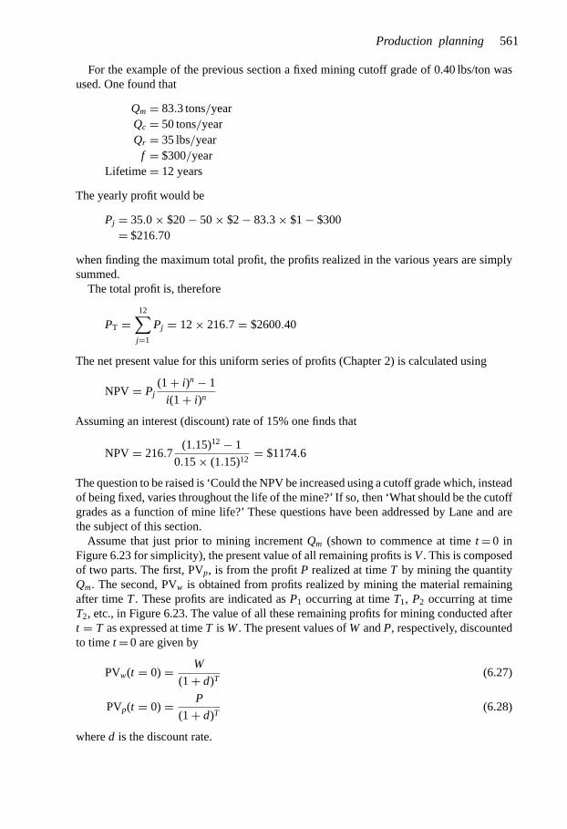
Production planning 561
For the example of the previous section a fixed mining cutoff grade of 0.40 lbs/ton wasused. One found that
Qm = 83.3 tons/yearQc = 50 tons/yearQr = 35 lbs/year
f = $300/yearLifetime = 12 years
The yearly profit would be
Pj = 35.0 × $20 − 50 × $2 − 83.3 × $1 − $300= $216.70
when finding the maximum total profit, the profits realized in the various years are simplysummed.
The total profit is, therefore
PT =12∑
j=1
Pj = 12 × 216.7 = $2600.40
The net present value for this uniform series of profits (Chapter 2) is calculated using
NPV = Pj(1 + i)n − 1
i(1 + i)n
Assuming an interest (discount) rate of 15% one finds that
NPV = 216.7(1.15)12 − 1
0.15 × (1.15)12= $1174.6
The question to be raised is ‘Could the NPV be increased using a cutoff grade which, insteadof being fixed, varies throughout the life of the mine?’ If so, then ‘What should be the cutoffgrades as a function of mine life?’ These questions have been addressed by Lane and arethe subject of this section.
Assume that just prior to mining increment Qm (shown to commence at time t = 0 inFigure 6.23 for simplicity), the present value of all remaining profits is V . This is composedof two parts. The first, PVp, is from the profit P realized at time T by mining the quantityQm. The second, PVw is obtained from profits realized by mining the material remainingafter time T . These profits are indicated as P1 occurring at time T1, P2 occurring at timeT2, etc., in Figure 6.23. The value of all these remaining profits for mining conducted aftert = T as expressed at time T is W . The present values of W and P, respectively, discountedto time t = 0 are given by
PVw(t = 0) = W
(1 + d)T(6.27)
PVp(t = 0) = P
(1 + d)T(6.28)
where d is the discount rate.

562 Open pit mine planning and design: Fundamentals
V � PVP � PVW
PVW
PVP
P
T0
P1
T1 T2 T3 TN
P2 P3 PN
V
W
Figure 6.23. A diagrammatic representation of the NPV calculation.
The present value at time t = 0 is therefore
V = W
(1 + d)T+ P
(1 + d)T(6.29)
Since the present value at time t = T of the remaining reserves is W , the difference vbetween the present values of the remaining reserves at times t = 0 and t = T is
v = V − W (6.30)
Equation (6.29) can be rewritten as
W + P = V (1 + d)T (6.31)
Applying the binomial expansion to the term (1 + d)T one finds that
(1 + d)T = 1 + Td + T(T − 1)d2
2! + T (T − 1)(T − 2)d3
3! + · · · (6.32)
For d small, (1 + d)T can be approximated by
(1 + d)T ≈ 1 + Td (6.33)
Combining Equations (6.31) and (6.33) results in
W + P = V (1 + Td) = V + VTd
or
V − W = P − VTd (6.34)
Comparing Equations (6.30) and (6.34) one finds that
v = P − VTd (6.35)
The profit P obtained through the mining of Qm in time T is given as before by
P = (s − r)Qr − cQc − mQm − f T (6.36)
Combining Equations (6.35) and (6.36) yields
v = (s − r)Qr − cQc − mQm − T ( f + Vd) (6.37)

Production planning 563
One would now like to schedule the mining in such a way that the decline in remainingpresent value takes place as rapidly as possible. This is because later profits get discountedmore than those captured earlier. In examining Equation (6.37), this means that v shouldbe maximized. As in the previous section one first takes the derivative of v with respect tograde. Setting the derivative equal to zero, one can solve for the appropriate cutoff gradessubject to mining, concentrating and refining constraints.
Step 1. Determination of the economic cutoff grades – one operation constraining the totalcapacity
(a) Calculate cutoff grade assuming that the mining rate is the governing constraint.The time Tm is given by
Tm = Qm
M(6.38)
Substituting this into Equation (6.37) yields
vm = (s − r)Qr − cQc −[m + f + Vd
M
]Qm (6.39)
Differentiating (6.39) with respect to grade g gives
dvm
dg= (s − r)
dQr
dg− c
dQc
dg−
[m + f + Vd
M
]dQm
dg(6.40)
However the quantity mined Qm does not depend upon the grade:
dQm
dg= 0 (6.41)
Hencedvm
dg= (s − r)
dQr
dg− c
dQc
dg(6.42)
The relationship between the quantities refined Qr and those sent for concentration Qc is
Qr = Qcgcy (6.43)
where gc is the average grade of ore sent for concentration and y is the recovery inconcentration.
ThusdQr
dg= gcy
dQc
dg(6.44)
Substituting Equation (6.44) into (6.42) yields
dvm
dg= [
(s − r)gcy − c] dQc
dg(6.45)
The average grade gc is defined as the mining cutoff (breakeven) grade gm when
dvm
dg= 0 (6.46)
Setting Equation (6.45) equal to zero and solving for gc = gm one finds that
gm = c
(s − r)y(6.47)
pjw
stk|
4020
64|1
4356
0354
9

564 Open pit mine planning and design: Fundamentals
Substituting the values from the example yields
gm = $2
($25 − $5)1.0= 0.10 lbs/ton
(b) Calculate cutoff grade assuming that the concentrating rate is the governing constraint.If the concentrator throughput rate is the limiting factor then the time T is controlled by theconcentrator.
T = Qc
C(6.48)
where Qc is the total number of tons which will be sent to the concentrator, and C is thetons/year capacity.
Equation (6.37) becomes
vc = (s − r)Qr − cQc − mQm − ( f + dV )Qc
C(6.49)
vc = (s − r)Qr − c + f + dV
CQc − mQm − m (6.50)
Since the total amount of material Qm is fixed,
mQm = const
Thus the cutoff grade affects only Qr and Qc.
Substituting as before
Qr = Qcgcy
one finds that
vc =[(s − r)gcy −
(c + f + dV
C
)]Qc − mQm (6.51)
To make vc as large as possible the term
(s − r)gcy −(
c + f + dV
C
)should be as large as possible. At breakeven (the cutoff grade), the term is zero. Thus
gc = c + f +dVC
y(s − r)(6.52)
(c) Calculate cutoff grade assuming the refining rate is the governing constraint. If therefinery output is the limiting factor then the time T is controlled by the refinery,
T = Qr
R(6.53)
where Qr is output of the refinery and R is the refining/sales capacity per year.Substituting into Equation (6.37) yields
vr = (s − r)Qr − cQc − mQm − ( f + dV )Qr
R(6.54)
vr =(
s − r − f + dV
R
)Qr − cQc − mQm (6.55)

Production planning 565
As before
Qr = gryQc
Thus
vr =(
s − r − f + dV
R
)gryQc − cQc − mQm
The total amount of material in the pit is fixed, therefore
mQm = const
Maximizing the expression for Vr one finds that(s − r − f + dV
R
)gryQc = cQc
Solving yields
gr = c(s − r − f +dV
R
)y
(6.56)
In summary, this first type of cutoff grade determination is based upon finding the grade forwhich the net increase in overall present value is zero. The expressions are as in formulas(6.47), (6.52) and (6.56):
gm = c
(s − r)y
gc = c + f +dVC
y(s − r)
gr = c(s − r − f +dV
R
)y
As can be seen, the expressions for gc and gr contain the unknown value of V .
Step 2. Determination of the economic cutoff grade by balancing the operationsThis step is exactly the same as that discussed in the previous section. Hence only the resultswill be presented here.
gmc = 0.50gcr = 0.60gmr = 0.456
Step 3. Determining the optimum of the six cutoff gradesThere are six possible cutoff grades. Three are based simply upon the grade distribution ofthe mined material and capacities.
gmc = 0.50gcr = 0.60gmr = 0.456

566 Open pit mine planning and design: Fundamentals
The other three are based upon capacities and cost/price. Substituting in the known valuesone finds that
gm = 0.10
gc = c + f + dVc
y(s − r)= 2 + 300 + 0.15V
50
1.0(25 − 5)
= 8 + 0.003V
20
gr = c(s − r − f + dV
R
)y
= 2(25 − 5 − 300 + 0.15V
40
)1.0
= 2
12.5 − 0.00375V
Of these, two of the limiting economic cut-off grades are not known initially since theydepend upon knowing the overall present value. This in turn depends upon the cutoff grade.Since the unknown V appears in the equations an iterative process must be used.
An optimum grade will be determined for each of the three pairs of operations. This willbe followed by finding the optimum of the three final candidates. For the mine and theconcentrator considered as a pair, there are three possible candidates for the optimum cutoffgrade Gmc. These are gm, gc, and gmc. The following rules are used to select Gmc.
Gmc =
gm ifgmc ≤ gm
gc ifgmc ≥ gc
gmc otherwise
This simple sorting algorithm yields the middle value. Treating the concentrator and refineryas a pair, the optimum Grc is found from
Grc =
gr ifgrc ≤ gr
gc ifgrc ≥ gc
grc otherwise
Finally the optimum cutoff grade Gmr when the mine and refinery are treated as a pair is
Gmr =
gm ifgmr ≤ gm
gr ifgmr ≥ gr
gmr otherwise
As the first step in the iteration process, it will be assumed that V = 0.Applying these rules to the example values
gm = 0.10gc = 0.40gr = 0.16
gmc = 0.50grc = 0.60gmr = 0.456

Production planning 567
Table 6.25. Concentrator product as a function of concentrator cutoff grade with mine operating atcapacity.
Concentrator Concentrator Average feed Concentrator/refinerycutoff feed grade product(lbs/ton) (tons) (lbs/ton) (lbs)
0.0 100 0.50 500.1 90 0.55 49.50.2 80 0.60 480.3 70 0.65 45.50.4 60 0.70 420.5 50 0.75 37.50.6 40 0.80 320.7 30 0.85 25.50.8 20 0.90 180.9 10 0.95 9.51.0 0 1.00 0
one finds that
Gmc = 0.40Grc = 0.40Gmr = 0.16
The overall optimum cutoff grade G is the middle value of Gmc, Gmr , and Grc.
G = middle value (Gmc, Gmr , Grc)
In this case
G = 0.40
Step 4. Calculation of quantitiesThe next step in the procedure is to determine the maximum quantities Qm, Qc and Qr
which could be produced and not violate the capacities. Assume that 100 tons are mined(Qm = 100). The grade distribution of this material is as shown in Table 6.24.
From Table 6.25, a cutoff grade of 0.40 would yield an average feed grade of 0.70. Each ofthe capacities must, however, be considered. A mining capacity (Qm = M) of 100 tons wouldmean 60 tons to the concentrator and 42 product units. Both the concentrator and refinerycapacities are exceeded. In meeting the concentrator capacity (Qc = 50), the required miningand refinery capacities are:
Qm = 5
6× 100 = 83.3
Qr = 50 × 0.70 = 35
These are both less than the maximum values. In meeting the refinery capacity of Qr = 40,the required concentrating and mining capacities are:
Qc = 40
0.7= 57.1
Qm = 57.1
60100 = 95.2
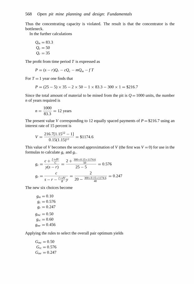
568 Open pit mine planning and design: Fundamentals
Thus the concentrating capacity is violated. The result is that the concentrator is thebottleneck.
In the further calculations
Qm = 83.3Qc = 50Qr = 35
The profit from time period T is expressed as
P = (s − r)Qr − cQc − mQm − f T
For T = 1 year one finds that
P = (25 − 5) × 35 − 2 × 50 − 1 × 83.3 − 300 × 1 = $216.7
Since the total amount of material to be mined from the pit is Q = 1000 units, the numbern of years required is
n = 1000
83.3= 12 years
The present value V corresponding to 12 equally spaced payments of P = $216.7 using aninterest rate of 15 percent is
V = 216.7[1.1512 − 1]
0.15(1.15)12= $1174.6
This value of V becomes the second approximation of V (the first was V = 0) for use in theformulas to calculate gc and gr .
gc = c + f +dVC
y(s − r)= 2 + 300+0.15×1174.6
50
25 − 5= 0.576
gr = c
s − r − f +dVR y
= 2
20 − 300+0.15×1174.640
= 0.247
The new six choices become
gm = 0.10gc = 0.576gr = 0.247
gmc = 0.50grc = 0.60gmr = 0.456
Applying the rules to select the overall pair optimum yields
Gmc = 0.50Grc = 0.576Gmr = 0.247

Production planning 569
The overall optimum is the middle value
G = 0.50
Returning to the grade distribution Table 6.24 one finds that the average grade is 0.75. If themining rate Qm = 100, then Qc = 50 and Qr = 37.5. Both the mine and the concentrator areat their rated capacities.
The profit in a given year is
P = (s − r)Qr − cQc − mQm − f T
= 20 × 37.5 − 2 × 50 − 1 × 100 − 300
= $250
The number of years is
n = Q
Qm= 1000
100= 10 years
The present value becomes
V = 2501.1510 − 1
0.15 × 1.1510= $1254.7
This becomes the third estimate for V to be used in calculating gc and gr .
gc = 2 + 300+0.15×1254.750
20= 0.588
gr = 2
20 − 300+0.15×1254.740
= 0.257
The six possible values are:
gm = 0.10gc = 0.588gr = 0.257
gmc = 0.50grc = 0.60gmr = 0.456
The optimum pairs are:
Gmc = 0.50Grc = 0.588Gmr = 0.257
and the overall optimum (G = 0.50) is the same as found with the previous estimate. Hencein year 1
Optimum cutoff grade = 0.50 lbs/tonQuantity mined = 100 tonsQuantity concentrated = 50 tonsQuantity refined = 37.5 lbsProfit = $250

570 Open pit mine planning and design: Fundamentals
Table 6.26. Reserve distribution at the end of year 1.
Grade (lbs/ton) Quantity (tons)
0.0–0.1 900.1–0.2 900.2–0.3 900.3–0.4 900.4–0.5 900.5–0.6 900.6–0.7 900.7–0.8 900.8–0.9 900.9–1.0 90
___Total = 900
Table 6.27. Reserve distribution at the start of year 8.
Grade (lbs/ton) Quantity (tons)
0.0–0.1 300.1–0.2 300.2–0.3 300.3–0.4 300.4–0.5 300.5–0.6 300.6–0.7 300.7–0.8 300.8–0.9 300.9–1.0 30
___Total = 300
The reserves must now be adjusted to those given in Table 6.25 and the process is repeatedassuming V = 0, calculating gc and gr , etc.
Through year 7, it will be found that the optimum cutoff grade remains at 0.50 with thequantities mined, concentrated and refined being 100, 50 and 37.5, respectively. The annualprofit is $250. The reserves going into year 8 are those given in Table 6.27. The balancinggrades remain at
gmc = 0.50grc = 0.60gmr = 0.456
The first approximation for the economic cutoff grades (V = 0) is
gm = 0.10gc = 0.40gr = 0.16
pjw
stk|
4020
64|1
4356
0355
3

Production planning 571
The optimum values of the pairs are
Gmc = Grc = 0.40Gmr = 0.16
The overall optimum is 0.40, and the quantities are
Qm = 83.3Qc = 50Qr = 35
The profit is $216.7 as before. The number of years becomes
n = 300
83.3= 3.6 years
The present value V becomes
V = 216.7(1.15)3.6 − 1
0.15(1.15)3.6= 571.2
Substituting this into the formulas for gc and gr yields
gc = 0.486gr = 0.193
Combining them with the others
gm = 0.10gmc = 0.50grc = 0.60gmr = 0.456
yields
Gmc = 0.486Grc = 0.486Gmr = 0.193
The overall optimum cutoff is G = 0.486 and the average grade above cutoff drops to 0.743:
Tons Grade Tons × Grade
4.2 0.493 2.0730 0.55 16.5030 0.65 19.5030 0.75 22.5030 0.85 25.5030 0.95 28.50____ _____ ______
Total = 154.2 Avg = 0.743 Sum = 114.57
There are 154.2 ore tons out of the 300 tons remaining to be mined. Since the concentratorcapacity is 50 tons/year, the mine life would be
n = 154.2
50= 3.08 years

572 Open pit mine planning and design: Fundamentals
Table 6.28. Reserve distribution at the start of year 9.
Grade (lbs/ton) Quantity (tons)
0.0–0.1 20.270.1–0.2 20.270.2–0.3 20.270.3–0.4 20.270.4–0.5 20.270.5–0.6 20.270.6–0.7 20.270.7–0.8 20.270.8–0.9 20.270.9–1.0 20.27______
Total = 202.27
The yearly mine production becomes
Qm = 300
3.08= 97.3
and Qr = 37.15. Calculating the profit one finds that
P = 20 × 37.15 − 2 × 50 − 1 × 97.3 − 300 = 245.7
The corresponding present value is
V = 245.7(1.15)3.08 − 1
0.15 × (1.15)3.08= $572.96
Repeating the process with this new estimate of V yields
gc = 0.486gr = 0.193
These are the same as before. Hence the values for year 8 are
G = 0.486Qm = 97Qc = 50Qr = 37.1
Profit = $245.7
The reserves are those given in Table 6.28. In year 9, the initial values for a cutoff of 0.4 are
Qm = 83.3Qc = 50Qr = 35
The profit would be $216.7.Based upon this mining rate, the reserves would last
n = 202.7
83.3= 2.43 years

Production planning 573
and the present value is
V = 216.7(1.15)2.43 − 1
0.15 × (1.15)2.43= $416.0
Recomputing gr and gc we obtain
gc = 0.462gr = 0.183
The other possible values are:
gm = 0.10gmc = 0.50grc = 0.60gmr = 0.456
The optimum pair values are:
Gmc = 0.462Grc = 0.462Gmr = 0.183
The middle value of these is
G = 0.462
Examining the reserve distribution suggests that there are 109.05 tons out of the total202.7 tons which are above cutoff. The average grade of this remaining ore is 0.731:
Tons Grade Tons × Grade
7.70 0.48 3.7020.27 0.55 11.1520.27 0.65 13.1820.27 0.75 15.2020.27 0.85 17.2320.27 0.95 19.26____ _____ _____
Total = 109.05 Avg = 0.731 Sum = 79.72
Since the maximum concentrating rate is 50 tons/year the life is
109.05
50= 2.18 years
The amount of product is
Qr = 50 × 0.731 = 36.55
Qm = 202.7
2.18= 93
The profit becomes
P = 20 × 36.55 − 2 × 50 − 1 × 93 − 300 = $238
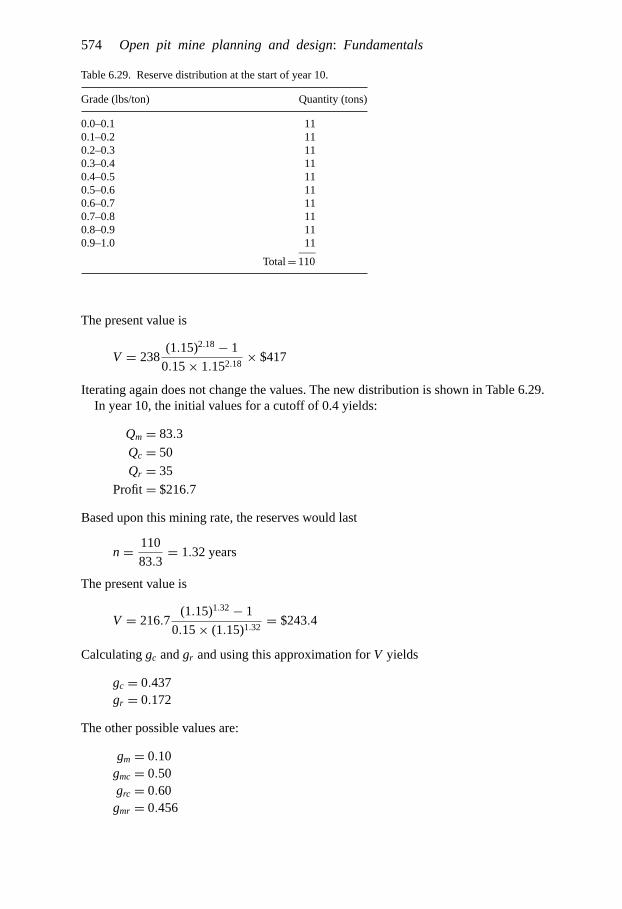
574 Open pit mine planning and design: Fundamentals
Table 6.29. Reserve distribution at the start of year 10.
Grade (lbs/ton) Quantity (tons)
0.0–0.1 110.1–0.2 110.2–0.3 110.3–0.4 110.4–0.5 110.5–0.6 110.6–0.7 110.7–0.8 110.8–0.9 110.9–1.0 11___
Total = 110
The present value is
V = 238(1.15)2.18 − 1
0.15 × 1.152.18× $417
Iterating again does not change the values. The new distribution is shown in Table 6.29.In year 10, the initial values for a cutoff of 0.4 yields:
Qm = 83.3
Qc = 50
Qr = 35
Profit = $216.7
Based upon this mining rate, the reserves would last
n = 110
83.3= 1.32 years
The present value is
V = 216.7(1.15)1.32 − 1
0.15 × (1.15)1.32= $243.4
Calculating gc and gr and using this approximation for V yields
gc = 0.437gr = 0.172
The other possible values are:
gm = 0.10gmc = 0.50grc = 0.60gmr = 0.456

Production planning 575
The optimum pair values are:
Gmc = 0.437Grc = 0.437Gmr = 0.172
The optimum value is G = 0.437. Examining the reserve distribution suggests that there are62 tons of the 110 tons remaining which are above this cutoff.
Tons Grade Tons × Grade
7 0.469 3.2811 0.55 6.0511 0.65 7.1511 0.75 8.2511 0.85 9.3511 0.95 10.45__ _____ _____
Total = 62 Avg = 0.718 Sum = 44.53
The average grade is 0.718. The number of years would be
n = 62
50= 1.24 years
The rate of mining and refining would be
Qm = 110
1.24= 89
Qr = 35.9
and the profit would become
P = 20 × 35.9 − 2 × 50 − 1 × 89 − 300
= $229
The present value is
V = $229(1.15)1.24 − 1
0.15 × (1.15)1.24= $243
Further iteration yields no change. In year 11, the grade distribution is shown in Table 6.30.The initial values (V = 0), yield a cutoff of 0.4 and
Qm = 21Qc = 12.6Qr = 8.8
The time would be the largest of
Tm = 21
100= 0.21
Tc = 12.6
50= 0.25
Tt = 8.8
40= 0.22

576 Open pit mine planning and design: Fundamentals
Table 6.30. Reserve distribution at the start of year 11.
Grade (lbs/ton) Quantity (tons)
0.0–0.1 2.10.1–0.2 2.10.2–0.3 2.10.3–0.4 2.10.4–0.5 2.10.5–0.6 2.10.6–0.7 2.10.7–0.8 2.10.8–0.9 2.10.9–1.0 2.1____
Total = 21.0
which is again controlled by the concentrator. The profit is
P = 20 × 8.8 − 12.6 × 2 − 21 × 1 − 300
4= $54.8
The present value is
V = $54.8(1.15)0.25 − 1
0.15 × (1.15)0.25= $12.5
Solving for gc and gr yields
gc = 0.402gr = 0.161
Combining with the others
gm = 0.16gmc = 0.50grc = 0.60gmr = 0.456
one finds that
Gmc = 0.402Grc = 0.402Gmr = 0.161
The cutoff grade is
G = 0.402
The distribution is only slightly changed and further iteration is not warranted.

Production planning 577
Table 6.31. The production schedule determined by the first pass.
Year Optimum Quantity Quantity Quantity Profit Net presentcutoff grade mined concentrated refined ($) value(lbs/ton) (tons) (tons) (lbs)
1 0.5 100 50 37.5 250 12552 0.5 100 50 37.5 250 11933 0.5 100 50 37.5 250 11224 0.5 100 50 37.5 250 10405 0.5 100 50 37.5 250 9466 0.5 100 50 37.5 250 8387 0.5 100 50 37.5 250 7148 0.486 97 50 37.1 245.7 5749 0.462 93 50 36.55 238 417
10 0.437 89 50 35.9 229 24311 0.40 21 12.6 8.8 55 53
Table 6.32. The final schedule for the manual example.
Year Optimum Quantity Quantity Quantity Profit Net presentcutoff grade mined concentrated refined ($) value(lbs/ton) (tons) (tons) (lbs)
1 0.50 100.0 50.0 37.5 250.0 1257.82 0.50 100.0 50.0 37.5 250.0 1196.53 0.50 100.0 50.0 37.5 250.0 1126.04 0.50 100.0 50.0 37.5 250.0 1044.95 0.50 100.0 50.0 37.5 250.0 951.76 0.50 100.0 50.0 37.5 250.0 844.57 0.50 100.0 50.0 37.5 250.0 721.18 0.49 97.2 50.0 37.1 245.6 579.39 0.46 93.0 50.0 36.6 238.2 420.6
10 0.44 88.7 50.0 35.9 229.5 245.511 0.41 21.0 12.5 8.8 54.7 52.8
The net present value is calculated using the yearly profits.
NPV = 250(1.15)7 − 1
0.15 × (1.15)7+ 245.7
(1.15)8+ 238
(1.15)9+ 229
(1.15)10+ 55
(1.15)10.25
= 1040 + 80.32 + 67.70 + 56.61 + 13.12
∼= $1258
Step 5. Repetition of the iteration processIn Table 6.31, the present value column reflects the current approximation to V as each yearscutoff grade was calculated. The present value of $1258 obtained using the yearly profitsshould be the same as that shown in the table for year 1. Since the values are not the same($1258 versus $1255), the process is repeated from the beginning using V = $1258 as theinitial estimate for V . Using a computer this iterative procedure is completed in fractionsof a second. The final results are shown in Table 6.32. The NPV is slightly higher than the$1255 which would have been obtained by maintaining a constant cutoff grade of 0.5.

578 Open pit mine planning and design: Fundamentals
In summary:– Initially the mine and the concentrator are in balance, both operating at capacity. In the
last few years, the concentrator is the limiter.– The cutoff grade begins at 0.50 lbs/ton and drops to 0.41 lbs/ton at the end of mine life.– Mine life is slightly more than 10 years.– Total copper produced = 380.9 lbs.– Total profits = $2518.– Net present value = $1257.80.This net present value should be compared to that of $1174.60 obtained with the fixed
cutoff grade.
6.8 MATERIAL DESTINATION CONSIDERATIONS
6.8.1 Introduction
The term ‘cutoff grade’ is a rather poorly defined term in the mining literature. A majorreason for this is that there are many different cutoff grades. Furthermore the values changewith time, mining progress, etc. A cutoff grade is simply a grade used to assign a destinationlabel to a parcel of material.
The destination can change. During the evaluation of final pit limits, the destinations tobe assigned are:
– to the surface, and– left in the ground.Once the destination ‘to the surface’ has been assigned, then the destination label ‘where
on the surface’ must be assigned as well. In the distant past there were really only twosurface destinations:
– to the mill, and– to the waste dump.A grade was used to assign the location. The distinction between destinations was called
the mill cutoff grade. In more recent times, the potential future value of material carryingvalues has been recognized. Hence the lean (low grade) ore dump has become a destination.Thus the 3 destinations require 2 distinguishing grades:
Destination Assignment– to the mill
mill cutoff grade
}– to the lean ore dump }
waste cutoff grade– to the waste dump
Today there are many more possible destinations as our ability to handle and treat materialshave improved. Leach dumps/leach pads are a common destination. An active stockpile isa less common destination.
This section will deal with alternate destinations to the mill and waste dump. These willbe discussed with respect to cutoff grade. However the reader should remember that thesesimply are a way of assigning material destinations.

Production planning 579
6.8.2 The leach dump alternative
For copper minerals and some others as well, the leach dump (or pad) is an alternativedestination to the mill or waste dump. Although this section will focus on copper, theapproach used is typical. Two cutoff grades must be determined:
1. Waste dump – leach cutoff.2. Leach dump – mill cutoff.
In one copper leaching process, sulfuric acid is percolated through the dump. The copperis taken into solution as cupric sulfate or cuprous sulfate. The collected solution is then runthrough a pachuca tank containing shredded iron where the iron goes into solution and thecopper is precipitated. The reactions are given below:
Dump
Leach material + H2SO4 → CuSO4 or Cu2SO4
Pachuca tank
CuSO4 + Fe → Cu + FeSO4 · H2O
The precipitated copper is then sent to the smelter. A full discussion of copper recovery fromdump material is far beyond the scope of this book. The rate of recovery and the overallpercent recovery depend upon both the ore and waste minerals present, the type of sprinklingand collection system, the size distribution of the particles involved, the way the material wasplaced, etc. Here the results presented by Davey (1979c) will be used for illustrative purposes.
For copper mineralization type 1, no recovery is expected when the copper content isbelow 0.2%. Using mineral dressing terminology, this would be the ‘Fixed Tails’ limit.Thus, when considering material destinations, the waste dump – leach dump cutoff criteriawould be:
Waste dump destination: copper content < 0.2%
Leach dump destination: copper content ≥ 0.2%
There will be another cutoff grade above which all material should be sent to the mill.To determine this value one must look both at the total copper recovery through leachingand the recovery as a function of time. For copper mineralization type 1, a fairly uniformdistribution of the various grades may be assumed for the low grade material having a headgrade of 0.4% copper or less. In this case
Head grade ≤ 0.4%
the percent recovery is expressed by
Recovery = Head grade − Fixed tails limit
Head grade× 100% (6.57a)
If the head grade is better than 0.4%,
Head grade > 0.4%
then the copper recovery by leaching is 50%
Recovery = 50% (6.57b)
Four examples will be used to demonstrate the use of the recovery formula.

580 Open pit mine planning and design: Fundamentals
Table 6.33. Recovery factor as a function of year for the leachexample (Davey, 1979c).
Year Recovery factor
1 0.402 0.303 0.144 0.105 0.06
1. Head grade = 0.45% Cu
Recovery = 50%
Recovered copper = 0.45
100× 0.5 × 2000 = 4.5 lbs/ton
2. Head grade = 0.40% Cu
Recovery = 0.40 − 0.20
0.40× 100 = 50%
Recovered copper = 0.40
100× 0.5 × 2000 = 4.0 lbs/ton
3. Head grade = 0.30% Cu
Recovery = 0.30 − 0.20
0.30× 100 = 33.3%
Recovered copper = 0.30
100× 0.333 × 2000 = 2 lbs/ton
4. Head grade = 0.15% Cu
Recovery = 0%
Recovered copper = 0 lbs/ton
The copper is recovered from the ton of material over some period of time, normally severalyears. The amount recovered per year from the ton normally decreases with time as shownbelow.
Yearly recovery (lbs) = Recovery factor × Total lbs to be recovered (6.58b)
The factors are given in Table 6.33.For a copper ore running 0.55% (head grade), the amount of copper in situ is 11 lbs/ton.
Of this 5.5 lbs is expected to be recovered over the 5-year period. For year 1, one wouldexpect to recover
Year 1 copper recovered = 0.40 × 5.5 lbs = 2.20 lbs
For year 2 the result would be
Year 2 copper recovered = 0.30 × 5.5 lbs = 1.65 lbs
Table 6.34 summarizes the overall recovery.

Production planning 581
Table 6.34. Estimated recovery as a function of year (Davey, 1979c).
Year Estimated recovery (lbs/ton)
1 2.202 1.653 0.774 0.555 0.33____
Total = 5.50
To demonstrate the application, consider the following example for a leach ore running0.55% Cu. The costs of mining and transporting the mineral are assumed to be the same forboth the milling and leaching alternatives. Since the material will be removed from the pitin any case, these are considered as sunk costs. An interesting exercise for the reader is tocalculate the value of potential leach material when deciding the ultimate pit limits. As canbe seen in Table 6.35, the net value per ton of material when considered for dump leachingis $2.07.
The same process is repeated for the milling alternative. This is done in Table 6.36.As can be seen, the net value is now $2.75/ton of material treated. Obviously, the
destination of the material should be the mill.The process illustrated in Table 6.35 and 6.36 is repeated until a breakeven grade between
leaching and milling is found (see Figure 6.24). In this particular case it is 0.45% Cu. Materialcarrying grades above this level should be sent to the mill. Material grading between 0.2and 0.45% copper should go to the leach dump.
In this simplified calculation, two important considerations have been left out. The firstis the cost of capital associated with the mill. Inclusion of these costs will increase thebreakeven grade. However, possible by-product credits from gold, molybdenum, etc., whichwould be realized by milling and not leaching have not been included. Obviously, a moredetailed analysis would take into account both of these factors.
It may also be that the mill capacity is taken up with higher grade material. In such acase another destination, a stockpile, might be considered. Cutoff grades are involved in thedecision as well.
If these cutoff grades are applied to the tonnage-grade curve given in Figure 6.25, onefinds the following.
Class of material Grade % Tons Average grade* (%)
Mill ore ≥0.45 7.4 × 10⁶ 0.96Leach ore 0.20 < g < 0.45 3.4 × 10⁶ 0.33Waste ≤0.20 20.0 × 10⁶ –
*See Figure 6.26.In this particular case, the actual production results were
Class of material Tons Average grade % Cu
Mill ore 7.5 × 10⁶ 0.93Leach 6.4 × 10⁶ 0.35Waste 16.9 × 10⁶ –

582 Open pit mine planning and design: Fundamentals
Table 6.35. Economic analysis regarding the leaching of material containing 0.55% copper (Davey, 1979c).
$/ton of material
A. Production cost breakdown1. Precipitation cost
($0.20/lb of recovered copper)– Recovery = 5.5 lbs/ton– Precipitation cost = 5.5 × $0.20 = $1.10 $1.10– The precipitate runs 85% copper
2. Treatment cost $1.08Smelting($50/ton of precipitate)
– Ratio of concentration = 2000 × 0.85
5.5= 309.09
– Smelting cost/ton of leach material = $50
309.09= $0.16
– Recovery = 97.5%– Freight (smelter → refinery)
($50/ton of blister copper)
– Freight cost = 5.5 × 0.98
2000× $50 = $0.1351
Refining($130/ton of blister copper)
– Refining cost = 5.404
2000× $130 = $0.351
– Recovery = 99.7%Selling and delivery($0.01/lb Cu)
cost = 0.01 × 5.39 = $0.054General plant($0.07/lb Cu)
cost = 0.07 × 5.39 = $0.38
3. Total production cost $2.18
B. Revenue ($/ton of leach material)1. Total value of in situ saleable copper
(price $1.00/lb)5.39 lbs × $1/lb = $5.39(discount rate i = 0%)
2. Discounted value(discount rate = 12.5%)
Recovered DiscountedYear copper (lbs) value ($)1 2.15 1.922 1.62 1.283 0.75 0.534 0.54 0.345 0.32 0.18____
$4.25
3. In general no by-products are recovered.4. It has been assumed that costs and prices have inflated at the same rate.
C. Net value ($/ton) of leach materialNet value = Revenue − Costs
= $4.25 − $2.18 = $2.07
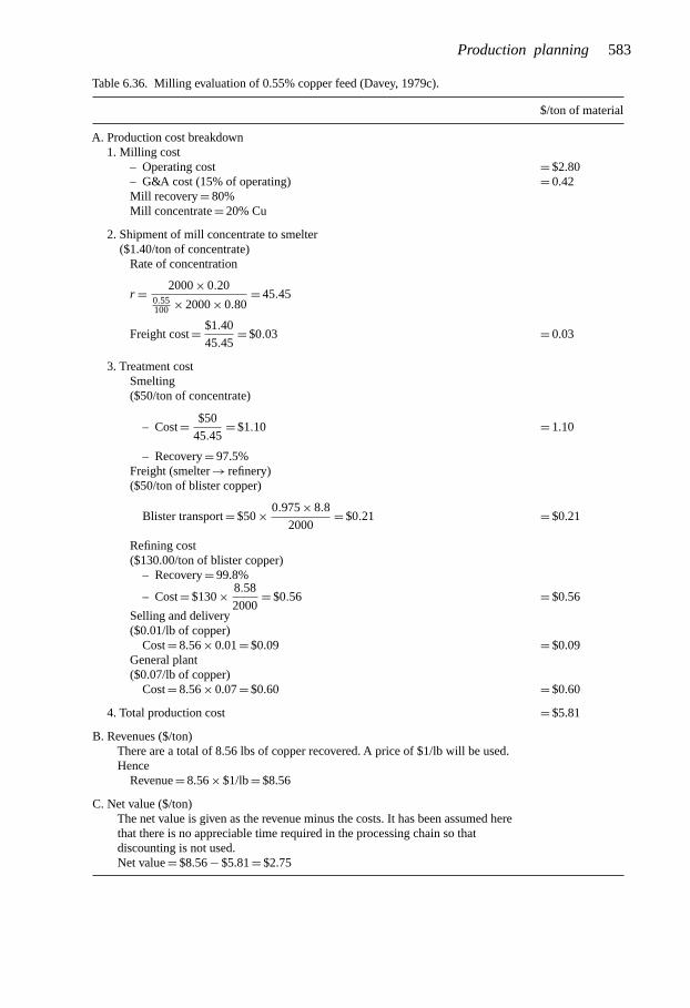
Production planning 583
Table 6.36. Milling evaluation of 0.55% copper feed (Davey, 1979c).
$/ton of material
A. Production cost breakdown1. Milling cost
– Operating cost = $2.80– G&A cost (15% of operating) = 0.42Mill recovery = 80%Mill concentrate = 20% Cu
2. Shipment of mill concentrate to smelter($1.40/ton of concentrate)
Rate of concentration
r = 2000 × 0.200.55100 × 2000 × 0.80
= 45.45
Freight cost = $1.40
45.45= $0.03 = 0.03
3. Treatment costSmelting($50/ton of concentrate)
– Cost = $50
45.45= $1.10 = 1.10
– Recovery = 97.5%Freight (smelter → refinery)($50/ton of blister copper)
Blister transport = $50 × 0.975 × 8.8
2000= $0.21 = $0.21
Refining cost($130.00/ton of blister copper)
– Recovery = 99.8%
– Cost = $130 × 8.58
2000= $0.56 = $0.56
Selling and delivery($0.01/lb of copper)
Cost = 8.56 × 0.01 = $0.09 = $0.09General plant($0.07/lb of copper)
Cost = 8.56 × 0.07 = $0.60 = $0.60
4. Total production cost = $5.81
B. Revenues ($/ton)There are a total of 8.56 lbs of copper recovered. A price of $1/lb will be used.Hence
Revenue = 8.56 × $1/lb = $8.56
C. Net value ($/ton)The net value is given as the revenue minus the costs. It has been assumed herethat there is no appreciable time required in the processing chain so thatdiscounting is not used.Net value = $8.56 − $5.81 = $2.75

584 Open pit mine planning and design: Fundamentals
0.300
1.00
1.67
2.00
Net
Val
ue (
$/to
n)3.00
Mill
Leach
0.35 0.40 0.45
Percent Copper (%)
0.550.50
Figure 6.24. Breakeven between milling and leaching.
6.8.3 The stockpile alternative
As has been discussed there are a series of cutoff grades which are applied during the lifeof a mine-mill complex. Early in the life, there is a desire to recover the capital investmentas early as possible. Since the mill capacity, in terms of tons per day, is normally fixed, itis better to use this capacity with higher rather than lower grade material. Hence the initialmill cutoff grade may be fairly high. As the mine-mill complex matures, the mill cutoffwill normally decrease. Assume that for a copper operation the set mill cutoff is 0.7% Cu.The mining cutoff (based upon covering the production costs, smelting, refining, sales,etc.) could be 0.3%. If the material has to be mined to reach deeper higher grade ore, thenthe breakeven cutoff for the mill destination could be even lower than 0.3%. As indicated,because of mill capacity restrictions and the requirement for rapid capital payback, the millcutoff is 0.7%. Therefore a large amount of material which, if produced later in the lifeof the mine would go to the mill, is now below cutoff. One possibility is to stockpile thematerial lying between 0.3% and 0.7% for later treatment by the mill. An alternative wouldbe to send the material to leach dumps for a quicker return of the costs expended in themining. No rehandling (with its added cost) would be required. Also there would not be acost associated with the storage areas themselves.

Production planning 585
00
2
4
6
Mill Ore
Leac
h O
re
Was
te
8
10
Tonn
age
(106
tons
)
12
14
16
18
0.5 1.0
Cutoff Grade (% Copper)
1.5 2.0 2.5 3.0
Figure 6.25. Superposition of the mill-leach and leach-waste cutoff grades on the Silver Bell oxide pitcumulative tonnage curve.
There are, in summary, a number of disadvantages with ore stockpiles (Schellman, 1989):1. A rehandling step is necessary. The costs involved may be significant.2. Space is required to accommodate the various qualities. Often such space is scarce
near the operations.3. Over time some materials become more difficult to treat.4. Additional expense is incurred in tracking the various qualities of material (sampling,
production control).For these and other reasons, stockpiles have not been popular with most mining operations.
There are some exceptions however.Taylor (1985) justified the use of the stockpile system through the use of some actual
examples from mines. At the Craigmont copper mine, a substantial sub-grade stockpilethat averaged about 0.6% Cu was accumulated from the initial high grade open pit. Theoperation then moved underground, where sublevel caving yielded a daily output of about

586 Open pit mine planning and design: Fundamentals
Cutoff Grade (% Copper)
00
0.5
0.5
1.0
1.0
0.20
0.45
1.5
1.5
2.0
2.0
2.5
2.5
Ave
rage
Gra
de (
% C
oppe
r)
3.0 3.5
3.0
4.0
3.5
4.5
Figure 6.26. Superposition of the mill-leach and leach-waste cutoff grades on the Silver Bell oxide pitaverage grade curve.
4500 tons at 1.8% Cu. For many years the stockpile provided the remaining 1500 tons perday that were needed to supply the mill. Another practical example is the Gibraltar coppermine. A cutoff grade of 0.3% Cu was used in the early years and more than 100,000,000short tons, grading down to 0.25% Cu, were stockpiled. In 1982–83 this surface ore enjoyeda cost advantage of at least $2.50 Canadian/ton over ore that had yet to be exposed in thepit. At the then low copper price, the 0.27% grade had a higher net value than the new0.37% Cu ore.
A leach dump is a form of stockpile since cutoff grades have been used to select thematerial for placement. Generally no rehandle is involved. Today a number of such ‘waste’dumps are being retreated with improved technology and there is reason to believe that thisprocess will occur even for the ‘waste’ dumps being created today.
There are a number of advantages to having stockpiles:1. They can be used for blending to ensure a constant head grade to the mill. Normally
recoveries are higher when such fluctuations are low.2. They can be used as a buffer to make up for production short falls due to various
reasons.

Production planning 587
Wastedump
71
Wastedump
57
Wastedump
67
Mill
Mine sulfidestockpile
Figure 6.27. Schematic representation ofvarious material destination (Schellman,1989).
3. The metal recovery is generally far higher in the mill than in the leach dump. Thusresource utilization is better. Since the overall recovery is higher the overall costs get spreadover a bigger base.
4. The presence of a buffer offers more flexibility in examining design options. Forexample one haulage road might be used instead of two due to the production securityprovided by the buffer. Steeper pit slopes might be considered.
In the future it is expected that the use of stockpiles will play a much more important partin the life of mines.
Computerized truck dispatching has simplified the changing of destinations. As can beseen in Figure 6.27, the dumping points are the concentrator plant, the three waste dumps(71, 57, and 67) and the sulfide stockpile. The addition of new dumps would not intro-duce major changes in the loading-haulage operation. Strategies regarding the number andtypes of stockpiles as well as how to best incorporate the stockpile into the overall oper-ating plan (when and how much to draw as compared to primary production) must bedeveloped.
Lane (1988) has provided a rather complete discussion regarding use of the stockpilealternative.
Schellman (1989) recently modified Lane’s algorithm to include the stockpiling optionwith the grades below current mill cutoff being segregated. The optimum time to draw uponthe stockpile as well as the tons and grades moved have been determined for three options.His approach will be illustrated using the data given in Table 6.37.
There are a total of 600 × 106 tons to be mined (100 × 106 tons in each phase). Thecapacities and costs used in applying the standard Lane approach described in Section 6.7are given in Table 6.38. The results without stockpiling are given in Table 6.39. As can beseen the total profits (PT ) are $484.2 × 10⁶ and the net present value (NPV) is $150.33 × 10⁶.Of the total tonnage mined 319 × 106 goes to the mill and the remainder 281 × 106 tons tothe waste dump. The cutoff grade in the final year is 0.23% Cu.
In the proposed system, a series of stockpiles are generated with material which is belowthe cutoff grade for each period but above the lowest cutoff grade for the whole project.Considering only increment 1 in the preceding example (Table 6.39), all material below0.5% and above 0.23% will be sent to the stockpile. For the second increment (year 6),material below 0.53% and above 0.23% will be sent to the stockpile.
Three different alternatives for handling the stockpiled material will be considered.

588 Open pit mine planning and design: Fundamentals
Table 6.37. Input data for the demonstration example (Lane, 1964) (The material amounts given are in 106
tons).
Grade Pit increments in mining sequencecategories(%Cu) 1 2 3 4 5 6
0.00–0.15 14.4 15.9 17.9 20.3 23.4 27.70.15–0.20 4.6 5.1 5.5 6.3 7.2 8.30.20–0.25 4.4 4.9 5.4 6.0 6.7 7.70.25–0.30 4.3 4.7 5.3 5.6 6.4 7.30.30–0.35 4.2 4.5 4.9 5.5 6.2 6.70.35–0.40 4.1 4.4 4.7 5.3 5.6 6.30.40–0.45 3.9 4.3 4.6 4.9 5.4 5.70.45–0.50 3.8 4.1 4.5 4.8 5.1 5.30.50–0.55 3.7 3.9 4.2 4.5 4.6 4.70.55–0.60 3.6 3.8 3.9 4.2 4.4 4.30.60–0.65 3.4 3.6 3.8 3.9 4.0 3.70.65–0.70 3.3 3.5 3.7 3.7 3.6 3.3+0.70 42.3 37.5 31.6 25.0 17.4 9.0Average % Cu 1.13 1.07 1.00 0.93 0.87 0.80
Table 6.38. Capacities and costs used in the demonstration example (Lane, 1964).
Capacities:Mine 20 million tons material/yearMill 10 million tons ore/yearRefinery 90,000 tons product/year
Costs:Mining $0.50/ton of material from pitMill $0.60/ton of ore to millRefining $50.0/ton of productFixed charges $4 million/yearSelling price $550/ton of productRecovery 90%
Alternative A. Mill feed coming simultaneously from the mine and stockpileIn this alternative, the analysis of whether or not to send material from the stockpile to the millis done taking into account the profit generated by the material in the stockpile and the profitgenerated by the material in the push back (pit increment). If the profitability of the ore in thestockpile is greater than that of the ore in the mine, ore from both the stockpile and the minewill feed the mill. The comparison is established between the same grade categories for bothalternatives. If, for example, at the mine the mineral grades between 0.4% and 0.7% and atthe stockpile it grades between 0.4% and 0.55%, only the mineral between 0.4% and 0.55%will be examined. If the profitability of the stockpiled ore is better, then ore between 0.4%and 0.55% will be sent from the stockpile. Ore with grades between 0.55% and 0.7% will besent from the mine. Mined material between 0.23% and 0.55% would be sent to the stockpile.
This stockpile system is dynamic, in the sense that, for some determined year, the stockpile is receiving ore from the mine, and sending ore to the mill. When the mining of the

Production planning 589
Table 6.39. Final production schedule for the demonstration example (Schellman, 1989).
Year Pit Cutoff Quantity Quantity Quantity Profit Total Net presentincrement grade mined concentrated refined (106 $) profit value
(% Cu) (106 tons) (106 tons) (106 tons) (106 $) (106 $)
1 1 0.50 17.9 10.0 90.0 26.1 484.2 150.332 1 0.50 17.9 10.0 90.0 26.1 458.1 146.803 1 0.50 17.9 10.0 90.0 26.1 432.0 142.754 1 0.50 17.9 10.0 90.0 26.1 405.9 138.085 1 0.50 17.9 10.0 90.0 26.1 379.8 132.726 1 0.50 10.7 6.0 54.2 15.7 353.7 126.556 2 0.53 8.0 4.0 34.2 9.1 338.0 126.557 2 0.5 20.0 10.0 85.9 23.0 328.9 120.698 2 0.53 20.0 10.0 85.9 23.0 305.9 115.839 2 0.53 20.0 10.0 85.9 23.0 282.9 110.23
10 2 0.53 20.0 10.0 85.9 23.0 259.9 103.8011 2 0.53 20.0 10.0 85.9 23.0 259.9 103.8011 3 0.47 7.8 3.9 29.5 7.0 222.8 96.4012 3 0.47 20.0 10.0 76.1 18.0 215.8 89.8013 3 0.47 20.0 10.0 76.1 18.0 197.8 85.2214 3 0.47 20.0 10.0 76.1 18.0 178.8 79.9515 3 0.47 20.0 10.0 76.4 18.0 161.8 73.9016 3 0.45 12.3 6.4 47.7 11.3 143.8 66.9416 4 0.41 7.2 3.6 24.0 4.8 132.5 66.9417 4 0.41 20.0 10.0 66.5 13.2 127.7 60.8718 4 0.41 20.0 10.0 66.5 13.2 114.5 56.7719 4 0.40 19.4 10.0 65.6 13.1 101.3 52.0620 4 0.38 18.8 10.0 64.5 12.9 88.2 46.7821 4 0.33 14.6 8.1 51.2 10.2 75.3 40.9121 5 0.35 3.8 1.9 11.0 1.7 65.3 40.9122 5 0.34 19.5 10.0 56.5 8.5 63.5 35.1823 5 0.33 19.0 10.0 55.8 8.4 55.0 31.9224 5 0.32 18.4 10.0 55.1 8.3 46.5 28.2725 5 0.30 17.9 10.0 54.3 8.2 38.1 24.1726 5 0.29 17.3 10.0 53.3 8.0 29.9 19.627 5 0.27 4.2 2.5 13.1 2.0 21.8 14.5027 6 0.27 14.1 7.5 34.7 2.8 20.3 14.5028 6 0.26 18.3 10.0 45.7 3.7 17.3 11.9129 6 0.26 18.0 10.0 45.4 3.7 13.6 10.0030 6 0.25 17.7 10.0 44.9 3.6 9.9 7.8331 6 0.24 17.3 10.0 44.4 3.6 6.3 5.3932 6 0.23 14.6 8.7 37.9 3.0 2.7 2.63
particular push back is completed, then the process continues. The stockpile would beconsidered as a new push back.
Alternative BIn this alternative if the profit from the ore in the stockpile is greater than that for ore in thepush back, the mill is fed with material exclusively coming from the stockpile.
The material to feed the mill is sent either from the stockpile or from the push back, butnot from both places simultaneously.

590 Open pit mine planning and design: Fundamentals
Alternative CIn this alternative, material is not sent to the mill from the stockpile during the mining of thepit. Material is stockpiled until all the material in the pit is exhausted. Only at that momentdoes the stockpile start to work as if it were a new push back.
The three stockpile alternatives will now be applied to the earlier example. The costinvolved with the stockpile is assumed to be $0.225/ton. This is 45% of the original min-ing cost. This incremental cost is $0.20/ton to cover material re-handling and $0.025/tonfor increased pit supervision, sampling, etc. The results from alternative A are given inTable 6.40. As can be seen the total profit is significantly higher than the no stockpile alter-native. The NPV is only slightly higher because the major contribution occurs late in thelife of the property. Table 6.41 is a year-by-year breakdown of the stockpile content. Thisis theoretical since one clearly would not keep so many separate grade categories.
The results from alternative B are shown in Table 6.42. As can be seen the NPV and theundiscounted profits are better than without stockpiling, but not as good as for alternativeA. This is because the stockpile only starts to send ore to the mill in year 28. In the previousalternative, the first time that the stockpile sends ore to the mill is in year 15. Moreover,using material from the stockpile in years 28 through 35 means that almost all of the materialin the stockpile is used. At the end of year 40, mining the remaining material in the stockpileis not economically profitable even though there is material in the stockpile between thegrades of 0.23% and 0.26%.
Alternative C (Table 6.43) has a better net present value and a better undiscounted profitthan without stockpiling. This alternative also has a slightly higher net present value thanalternative B, but smaller than alternative A. From an operational point of view, this alter-native has several advantages. It is not necessary to blend material as in the productionschedule generated by alternative A or to stop the mine production for 8 years and then startto produce again, as in alternative B.
The stockpile option should always be considered in open pit mine planning. The potentialcontribution to the NPV depends upon each particular case. It is particularly dependentupon the spread between the highest and the lowest grades in the project cutoff gradestrategy. If that spread is significant, the stockpile alternative should be considered for theproject.
6.9 PRODUCTION SCHEDULING
6.9.1 Introduction
Production scheduling is a very important part of the mining process. This will be demon-strated through a simple example. Consider the property shown in Figure 6.28 in which 10ore blocks are overlain by 10 waste blocks.
A production rate of 5 blocks per year (irrespective of whether the blocks are ore orwaste) will be assumed. The net value for an ore block is $2 and the cost of removing thewaste is $1/block. The total cost involved in waste removal would be $10 and the ore valueis $20.
If both ore and waste could be mined instantaneously, the net present value would be$10. However due to practical constraints, they cannot. Therefore a number of schedulingscenarios must be considered.

Production planning 591
Table 6.40. Final schedule for the alternative A stockpile (Schellman, 1989).
Year Pit Cutoff Quantity Quantity Quantity Profit Total Net presentincrement grade mined concentrated refined (106 $) profit value
(% Cu) (106 tons) (106 tons) (106 tons) (106 $) (106 $)
1 1 0.50 17.8 10.0 89.8 26.0 528.4 150.562 1 0.50 17.8 10.0 89.8 26.0 502.4 147.133 1 0.50 17.8 10.0 89.8 26.0 476.4 143.194 1 0.50 17.8 10.0 89.8 26.0 450.4 138.665 1 0.50 17.8 10.0 89.8 26.0 424.4 133.456 1 0.50 11.2 6.3 56.6 16.4 398.4 127.466 2 0.53 7.4 3.7 31.8 8.5 382.0 127.467 2 0.53 20.0 10.0 85.9 23.0 373.5 121.698 2 0.53 20.0 10.0 85.9 23.0 350.5 116.979 2 0.53 20.0 10.0 85.9 23.0 327.5 111.55
10 2 0.53 20.0 10.0 85.9 23.0 304.5 105.3111 2 0.53 12.8 6.4 55.0 14.7 281.5 98.1411 3 0.47 7.2 3.6 27.4 6.5 266.8 98.1412 3 0.47 20.0 10.0 76.1 18.0 260.3 91.6613 3 0.47 20.0 10.0 76.1 18.0 242.3 87.3614 3 0.47 20.0 10.0 76.1 18.0 224.3 82.4215 *** 0.47 1.0 10.0 4.6 1.2 206.3 76.7315 3 0.47 18.7 9.0 71.5 17.2 205.1 76.7316 3 0.47 13.1 6.4 48.8 11.4 187.9 69.8216 4 0.41 6.9 3.5 23.1 4.6 176.5 69.8217 4 0.41 20.0 10.0 66.5 13.2 171.9 64.2818 4 0.41 20.0 10.0 66.5 13.2 158.7 60.7019 4 0.41 20.0 10.0 66.5 13.2 145.5 56.5720 *** 0.41 2.2 2.2 9.2 2.2 132.3 51.8320 4 0.41 17.3 7.8 57.0 11.7 130.1 51.8321 4 0.41 13.6 6.6 43.8 8.4 118.4 45.6421 5 0.35 6.4 3.2 18.3 2.8 110.0 45.6422 5 0.35 20.0 10.0 57.2 8.6 107.2 41.3523 5 0.35 20.0 10.0 57.2 8.6 98.6 38.9424 5 0.35 20.0 10.0 57.2 8.6 90.0 36.1725 *** 0.35 3.7 3.7 15.4 3.7 81.4 32.9825 5 0.35 15.6 6.3 42.5 6.6 77.7 32.9826 5 0.35 14.7 7.2 40.5 5.6 71.1 27.6026 6 0.29 5.3 2.6 12.6 1.0 65.5 27.6027 6 0.29 20.0 10.0 47.6 3.8 64.5 25.0828 6 0.29 20.0 10.0 47.6 3.8 60.7 25.0329 6 0.29 20.0 10.0 47.6 3.8 56.9 24.9830 *** 0.29 5.5 5.5 18.8 3.6 53.1 24.9130 6 0.29 13.6 4.5 27.6 1.6 49.5 24.9131 6 0.29 16.0 7.8 36.7 2.5 47.9 23.5031 *** 0.31 2.2 2.2 6.8 0.8 45.6 23.5032 *** 0.31 10.0 10.0 36.5 6.0 44.6 23.7933 *** 0.30 10.0 10.0 36.5 6.0 38.6 21.3634 *** 0.29 10.0 10.0 35.1 5.3 32.6 18.5735 *** 0.28 10.0 10.0 34.5 5.0 27.3 16.0536 *** 0.27 10.0 10.0 33.7 4.6 22.3 13.4737 *** 0.27 10.0 10.0 32.9 4.2 17.7 10.9038 *** 0.26 10.0 10.0 30.8 3.1 13.5 8.3539 *** 0.25 10.0 10.0 29.0 2.3 10.4 6.4540 *** 0.24 10.0 10.0 27.2 1.4 8.1 5.1741 *** 0.23 10.0 10.0 27.2 1.4 6.7 4.5842 *** 0.23 10.0 10.0 27.2 1.4 5.3 3.9143 *** 0.23 10.0 10.0 28.2 1.9 3.9 3.1344 *** 0.23 8.2 8.2 24.2 2.0 2.0 1.7
*** Mineral from stockpile.

Table 6.41. Stockpile grade and tonnage (expressed in 106 tons) distribution by year for alternative A (Schellman, 1989).
STOCKPILE GRADE DISTRIBUTION STOCKPILE GRADE DISTRIBUTION STOCKPILE GRADE DISTRIBUTION STOCKPILE GRADE DISTRIBUTIONYEAR 1 YEAR 4 YEAR 7 YEAR 10
GRADE GRADE GRADE GRADECATEGORIES AVRG TONNAGE CATEGORIES AVRG TONNAGE CATEGORIES AVRG TONNAGE CATEGORIES AVRG TONNAGE% % % %.230 .250 .240 .5 .230 .250 .240 1.9 .230 .250 .240 3.2 .230 .250 .240 5.0.250 .300 .275 .8 .250 .300 .275 3.1 .250 .300 .275 5.2 .250 .300 .275 8.1.300 .350 .325 .7 .300 .350 .325 3.0 .300 .350 .325 5.1 .300 .350 .325 7.8.350 .400 .375 .7 .350 .400 .375 2.9 .350 .400 .375 5.0 .350 .400 .375 7.6.400 .450 .425 .7 .400 .450 .425 2.8 .400 .450 .425 4.8 .400 .450 .425 7.3.450 .500 .475 .7 .450 .500 .475 2.7 .450 .500 .475 4.6 .450 .500 .475 7.1
.500 .528 .514 .4 .500 .528 .514 1.8
TOTAL: 4.1 TOTAL: 16.3 TOTAL: 28.4 TOTAL: 44.6
STOCKPILE GRADE DISTRIBUTION STOCKPILE GRADE DISTRIBUTION STOCKPILE GRADE DISTRIBUTION STOCKPILE GRADE DISTRIBUTIONYEAR 2 YEAR 5 YEAR 8 YEAR 11
GRADE GRADE GRADE GRADECATEGORIES AVRG TONNAGE CATEGORIES AVRG TONNAGE CATEGORIES AVRG TONNAGE CATEGORIES AVRG TONNAGE% % % %.230 .250 .240 .9 .230 .250 .240 2.3 .230 .250 .240 3.8 .230 .250 .240 5.4.250 .300 .275 1.5 .250 .300 .275 3.8 .250 .300 .275 6.2 .250 .300 .275 8.7.300 .350 .325 1.5 .300 .350 .325 3.7 .300 .350 .325 6.0 .300 .350 .325 8.4.350 .400 .375 1.5 .350 .400 .375 3.6 .350 .400 .375 5.9 .350 .400 .375 8.2.400 .450 .425 1.4 .400 .450 .425 3.5 .400 .450 .425 5.6 .400 .450 .425 7.9.450 .500 .475 1.3 .450 .500 .475 3.4 .450 .500 .475 5.4 .450 .469 .459 2.9
.500 .528 .514 .9 .469 .500 .484 4.7.500 .528 .514 2.0
TOTAL: 8.1 TOTAL: 20.4 TOTAL: 33.8 TOTAL: 48.1
STOCKPILE GRADE DISTRIBUTION STOCKPILE GRADE DISTRIBUTION STOCKPILE GRADE DISTRIBUTION STOCKPILE GRADE DISTRIBUTIONYEAR 3 YEAR 6 YEAR 9 YEAR 12
GRADE GRADE GRADE GRADECATEGORIES AVRG TONNAGE CATEGORIES AVRG TONNAGE CATEGORIES AVRG TONNAGE CATEGORIES AVRG TONNAGE% % % %.230 .250 .240 1.4 .230 .250 .240 2.6 .230 .250 .240 4.4 .230 .250 .240 6.0.250 .300 .275 2.3 .250 .300 .275 4.3 .250 .300 .275 7.1 .250 .300 .275 9.7.300 .350 .325 2.2 .300 .350 .325 4.2 .300 .350 .325 6.9 .300 .350 .325 9.3.350 .400 .375 2.2 .350 .400 .375 4.1 .350 .400 .375 6.7 .350 .400 .375 9.1.400 .450 .425 2.1 .400 .450 .425 3.9 .400 .450 .425 6.5 .400 .450 .425 8.8.450 .500 .475 2.0 .450 .500 .475 3.8 .450 .500 .475 6.3 .450 .469 .459 3.2
.500 .528 .514 1.3 .469 .500 .484 4.7.500 .528 .514 2.0
TOTAL: 12.2 TOTAL: 22.9 TOTAL: 39.2 TOTAL: 53.0

Table 6.41. (Continued).
STOCKPILE GRADE DISTRIBUTION STOCKPILE GRADE DISTRIBUTION STOCKPILE GRADE DISTRIBUTION STOCKPILE GRADE DISTRIBUTIONYEAR 13 YEAR 16 YEAR 19 YEAR 22
GRADE GRADE GRADE GRADECATEGORIES AVRG TONNAGE CATEGORIES AVRG TONNAGE CATEGORIES AVRG TONNAGE CATEGORIES AVRG TONNAGE% % % %.230 .250 .240 6.7 .230 .250 .240 8.4 .230 .250 .240 10.5 .230 .250 .240 12.5.250 .300 .275 10.8 .250 .300 .275 13.6 .250 .300 .275 16.9 .250 .300 .275 20.1.300 .350 .325 10.3 .300 .350 .325 12.9 .300 .350 .325 16.2 .300 .350 .325 19.3.350 .400 .375 10.1 .350 .400 .375 12.5 .350 .400 .375 15.7 .350 .400 .375 17.5.400 .450 .425 9.7 .400 .410 .405 2.5 .400 .410 .405 3.1 .400 .410 .405 3.4.450 .469 .459 3.6 .410 .450 .430 9.7 .410 .450 .430 9.7 .410 .450 .430 9.4.469 .500 .484 4.7 .450 .469 .459 4.4 .450 .469 .459 4.4 .450 .469 .459 4.3.500 .528 .514 2.0 .469 .500 .484 4.6 .469 .500 .484 4.6 .469 .500 .484 5.1
.500 .528 .514 2.2 .500 .528 .514 2.2 .500 .528 .514 2.0
TOTAL: 57.9 TOTAL: 70.7 TOTAL: 83.3 TOTAL: 93.5
STOCKPILE GRADE DISTRIBUTION STOCKPILE GRADE DISTRIBUTION STOCKPILE GRADE DISTRIBUTION STOCKPILE GRADE DISTRIBUTIONYEAR 14 YEAR 17 YEAR 20 YEAR 23
GRADE GRADE GRADE GRADECATEGORIES AVRG TONNAGE CATEGORIES AVRG TONNAGE CATEGORIES AVRG TONNAGE CATEGORIES AVRG TONNAGE% % % %.230 .250 .240 7.3 .230 .250 .240 9.1 .230 .250 .240 11.2 .230 .250 .240 13.3.250 .300 .275 11.8 .250 .300 .275 14.7 .250 .300 .275 18.0 .250 .300 .275 21.3.300 .350 .325 11.3 .300 .350 .325 14.0 .300 .350 .325 17.3 .300 .350 .325 20.5.350 .400 .375 11.0 .350 .400 .375 13.6 .350 .400 .375 16.7 .350 .400 .375 17.5.400 .450 .425 10.6 .400 .410 .405 2.7 .400 .410 .405 3.3 .400 .410 .405 3.4.450 .469 .459 3.9 .410 .450 .430 9.7 .410 .450 .430 9.4 .410 .450 .430 9.4.469 .500 .484 4.7 .450 .469 .459 4.4 .450 .469 .459 4.3 .450 .469 .459 4.3.500 .528 .514 2.0 .469 .500 .484 4.6 .469 .500 .484 5.1 .469 .500 .484 5.1
.500 .528 .514 2.2 .500 .528 .514 2.0 .500 .528 .514 2.0
TOTAL: 62.7 TOTAL: 74.9 TOTAL: 87.2 TOTAL: 96.8
STOCKPILE GRADE DISTRIBUTION STOCKPILE GRADE DISTRIBUTION STOCKPILE GRADE DISTRIBUTION STOCKPILE GRADE DISTRIBUTIONYEAR 15 YEAR 18 YEAR 21 YEAR 24
GRADE GRADE GRADE GRADECATEGORIES AVRG TONNAGE CATEGORIES AVRG TONNAGE CATEGORIES AVRG TONNAGE CATEGORIES AVRG TONNAGE% % % %.230 .250 .240 7.9 .230 .250 .240 9.8 .230 .250 .240 11.7 .230 .250 .240 14.1.250 .300 .275 12.9 .250 .300 .275 15.8 .250 .300 .275 18.8 .250 .300 .275 22.6.300 .350 .325 12.3 .300 .350 .325 15.1 .300 .350 .325 18.0 .300 .350 .325 21.7.350 .400 .375 11.9 .350 .400 .375 14.7 .350 .400 .375 17.5 .350 .400 .375 17.5.400 .450 .425 11.5 .400 .410 .405 2.9 .400 .410 .405 3.4 .400 .410 .405 3.4.450 .469 .459 4.2 .410 .450 .430 9.7 .410 .450 .430 9.4 .410 .450 .430 9.4.469 .500 .484 4.6 .450 .469 .459 4.4 .450 .469 .459 4.3 .450 .469 .459 4.3.500 .528 .514 2.2 .469 .500 .484 4.6 .469 .500 .484 5.1 .469 .500 .484 5.1
.500 .528 .514 2.2 .500 .528 .514 2.0 .500 .528 .514 2.0
TOTAL: 67.5 TOTAL: 79.1 TOTAL: 90.2 TOTAL: 100.1

Table 6.41. (Continued).
STOCKPILE GRADE DISTRIBUTION STOCKPILE GRADE DISTRIBUTION STOCKPILE GRADE DISTRIBUTION STOCKPILE GRADE DISTRIBUTIONYEAR 25 YEAR 27 YEAR 29 YEAR 31
GRADE GRADE GRADE GRADECATEGORIES AVRG TONNAGE CATEGORIES AVRG TONNAGE CATEGORIES AVRG TONNAGE CATEGORIES AVRG TONNAGE% % % %.230 .250 .240 14.9 .230 .250 .240 16.4 .230 .250 .240 18.3 .230 .250 .240 19.9.250 .300 .275 23.8 .250 .293 .272 22.6 .250 .293 .272 25.2 .250 .293 .272 22.6.300 .350 .325 22.9 .293 .300 .297 3.4 .293 .300 .297 3.4 .293 .300 .297 3.3.350 .400 .375 18.5 .300 .350 .325 23.8 .300 .350 .325 23.8 .300 .350 .325 23.1.400 .410 .405 3.6 .350 .400 .375 18.5 .350 .400 .375 18.5 .350 .400 .375 18.2.410 .450 .430 8.5 .400 .410 .405 3.6 .400 .410 .405 3.6 .400 .410 .405 3.5.450 .469 .459 4.4 .410 .450 .430 8.5 .410 .450 .430 8.5 .410 .450 .430 8.6.469 .500 .484 4.8 .450 .469 .459 4.4 .450 .469 .459 4.4 .450 .469 .459 4.9.500 .528 .514 1.6 .469 .500 .484 4.8 .469 .500 .484 4.8 .469 .500 .484 5.0
.500 .528 .514 1.6 .500 .528 .514 1.6 .500 .528 .514 1.5.500 .528 .514 4.4.528 .550 .539 4.8
TOTAL: 103.0 TOTAL: 107.7 TOTAL: 112.0 TOTAL: 124.5
STOCKPILE GRADE DISTRIBUTION STOCKPILE GRADE DISTRIBUTION STOCKPILE GRADE DISTRIBUTION STOCKPILE GRADE DISTRIBUTIONYEAR 26 YEAR 28 YEAR 30 YEAR 32
GRADE GRADE GRADE GRADECATEGORIES AVRG TONNAGE CATEGORIES AVRG TONNAGE CATEGORIES AVRG TONNAGE CATEGORIES AVRG TONNAGE% % % %.230 .250 .240 15.5 .230 .250 .240 17.3 .230 .250 .240 19.1 .230 .250 .240 19.5.250 .293 .272 21.4 .250 .293 .272 23.9 .250 .293 .272 26.3 .250 .284 .267 21.3.293 .300 .297 3.4 .293 .300 .297 3.4 .293 .300 .297 3.3 .284 .293 .289 5.5.300 .350 .325 23.8 .300 .350 .325 23.8 .300 .350 .325 23.1 .293 .300 .297 3.2.350 .400 .375 18.5 .350 .400 .375 18.5 .350 .400 .375 18.2 .300 .350 .325 22.7.400 .410 .405 3.6 .400 .410 .405 3.6 .400 .410 .405 3.5 .350 .400 .375 17.9.410 .450 .430 8.5 .410 .450 .430 8.5 .410 .450 .430 8.6 .400 .410 .405 3.5.450 .469 .459 4.4 .450 .469 .459 4.4 .450 .469 .459 4.9 .410 .450 .430 8.5.469 .500 .484 4.8 .469 .500 .484 4.8 .469 .500 .484 5.0 .450 .469 .459 4.8.500 .528 .514 1.6 .500 .528 .514 1.6 .500 .528 .514 1.5 .469 .500 .484 4.9
.500 .528 .514 1.4
.500 .528 .514 4.3
.528 .550 .539 4.7
.550 .600 .575 1.6
TOTAL: 105.5 TOTAL: 109.8 TOTAL: 113.6 TOTAL: 123.9

Table 6.41. (Continued).
STOCKPILE GRADE DISTRIBUTION STOCKPILE GRADE DISTRIBUTION STOCKPILE GRADE DISTRIBUTIONYEAR 33 YEAR 35 YEAR 37
GRADE GRADE GRADECATEGORIES AVRG TONNAGE CATEGORIES AVRG TONNAGE CATEGORIES AVRG TONNAGE% % %.230 .250 .240 19.5 .230 .250 .240 19.5 .230 .250 .240 19.5.250 .278 .264 17.6 .250 .265 .258 9.4 .250 .261 .256 7.2.278 .284 .281 3.8 .265 .271 .268 4.0 .261 .265 .263 2.2.284 .293 .289 5.5 .271 .278 .275 4.2 .265 .271 .268 4.0.293 .300 .297 3.2 .278 .284 .281 3.8 .271 .278 .275 3.4.300 .350 .325 19.7 .284 .293 .289 4.7 .278 .284 .281 2.5.350 .400 .375 15.5 .293 .300 .297 2.7 .284 .293 .289 3.1.400 .410 .405 3.0 .300 .350 .325 14.0 .293 .300 .297 1.8.410 .450 .430 7.3 .350 .400 .375 11.0 .300 .350 .325 9.3.450 .469 .459 4.1 .400 .410 .405 2.1 .350 .400 .375 7.3.469 .500 .484 4.3 .410 .450 .430 5.2 .400 .410 .405 1.4.500 .528 .514 1.3 .450 .469 .459 2.9 .410 .450 .430 3.5.500 .528 .514 3.7 .469 .500 .484 3.0 .450 .469 .459 2.0.528 .550 .539 4.1 .500 .528 .514 .9 .469 .500 .484 2.0.550 .600 .575 1.4 .500 .528 .514 2.6 .500 .528 .514 .6
.528 .550 .539 2.9 .500 .528 .514 1.8
.550 .600 .575 1.0 .528 .550 .539 1.9.550 .600 .575 .7
TOTAL: 113.9 TOTAL: 93.9 TOTAL: 73.9
STOCKPILE GRADE DISTRIBUTION STOCKPILE GRADE DISTRIBUTION STOCKPILE GRADE DISTRIBUTIONYEAR 34 YEAR 36 YEAR 38
GRADE GRADE GRADECATEGORIES AVRG TONNAGE CATEGORIES AVRG TONNAGE CATEGORIES AVRG TONNAGE% % %.230 .250 .240 19.5 .230 .250 .240 19.5 .230 .245 .238 15.0.250 .271 .261 13.3 .250 .265 .258 9.4 .245 .250 .248 4.5.271 .278 .275 4.2 .265 .271 .268 4.0 .250 .261 .256 7.2.278 .284 .281 3.8 .271 .278 .275 4.2 .261 .265 .263 1.7.284 .293 .289 5.5 .278 .284 .281 3.1 .265 .271 .268 3.1.293 .300 .297 3.2 .284 .293 .289 3.8 .271 .278 .275 2.7.300 .350 .325 16.6 .293 .300 .297 2.3 .278 .284 .281 2.0.350 .400 .375 13.0 .300 .350 .325 11.5 .284 .293 .289 2.4.400 .410 .405 2.5 .350 .400 .375 9.1 .293 .300 .297 1.4.410 .450 .430 6.2 .400 .410 .405 1.8 .300 .350 .325 7.3.450 .469 .459 3.5 .410 .450 .430 4.3 .350 .400 .375 5.7.469 .500 .484 3.6 .450 .469 .459 2.4 .400 .410 .405 1.1.500 .528 .514 1.1 .469 .500 .484 2.5 .410 .450 .430 2.7.500 .528 .514 3.1 .500 .528 .514 .7 .450 .469 .459 1.5.528 .550 .539 3.4 .500 .528 .514 2.2 .469 .500 .484 1.6.550 .600 .575 1.2 .528 .550 .539 2.4 .500 .528 .514 .5
.550 .600 .575 .8 .500 .528 .514 1.4.528 .550 .539 1.5.550 .600 .575 .5
TOTAL: 103.9 TOTAL: 83.9 TOTAL: 63.9

Table 6.41. (Continued).
STOCKPILE GRADE DISTRIBUTION STOCKPILE GRADE DISTRIBUTION STOCKPILE GRADE DISTRIBUTIONYEAR 39 YEAR 41 YEAR 43
GRADE GRADE GRADECATEGORIES AVRG TONNAGE CATEGORIES AVRG TONNAGE CATEGORIES AVRG TONNAGE% % %.230 .245 .238 15.0 .230 .245 .238 9.5 .230 .245 .238 3.9.245 .250 .248 4.5 .245 .250 .248 2.8 .245 .250 .248 1.2.250 .261 .256 5.5 .250 .261 .256 3.5 .250 .261 .256 1.4.261 .265 .263 1.3 .261 .265 .263 .8 .261 .265 .263 .3.265 .271 .268 2.4 .265 .271 .268 1.5 .265 .271 .268 .6.271 .278 .275 2.1 .271 .278 .275 1.3 .271 .278 .275 .5.278 .284 .281 1.5 .278 .284 .281 1.0 .278 .284 .281 .4.284 .293 .289 1.9 .284 .293 .289 1.2 .284 .293 .289 .5.293 .300 .297 1.1 .293 .300 .297 .7 .293 .300 .297 .3.300 .350 .325 5.7 .300 .350 .325 3.6 .300 .350 .325 1.5.350 .400 .375 4.4 .350 .400 .375 2.8 .350 .400 .375 1.1.400 .410 .405 .9 .400 .410 .405 .5 .400 .410 .405 .2.410 .450 .430 2.1 .410 .450 .430 1.3 .410 .450 .430 .5.450 .469 .459 1.2 .450 .469 .459 .8 .450 .469 .459 .3.469 .500 .484 1.2 .469 .500 .484 .8 .469 .500 .484 .3.500 .528 .514 .4 .500 .528 .514 .2 .500 .528 .514 .1.500 .528 .514 1.1 .500 .528 .514 .7 .500 .528 .514 .3.528 .550 .539 1.2 .528 .550 .539 .7 .528 .550 .539 .3.550 .600 .575 .4 .550 .600 .575 .3 .550 .600 .575 .1
.431 .444 .438 2.9
TOTAL: 53.9 TOTAL: 33.9 TOTAL: 16.8
STOCKPILE GRADE DISTRIBUTION STOCKPILE GRADE DISTRIBUTION STOCKPILE GRADE DISTRIBUTIONYEAR 40 YEAR 42 YEAR 44
GRADE GRADE GRADECATEGORIES AVRG TONNAGE CATEGORIES AVRG TONNAGE CATEGORIES AVRG TONNAGE% % %.230 .245 .238 12.3 .230 .245 .238 6.7 .230 .245 .238 1.6.245 .250 .248 3.6 .245 .250 .248 2.0 .245 .250 .248 .5.250 .261 .256 4.5 .250 .261 .256 2.5 .250 .261 .256 .6.261 .265 .263 1.1 .261 .265 .263 .6 .261 .265 .263 .1.265 .271 .268 2.0 .265 .271 .268 1.1 .265 .271 .268 .3.271 .278 .275 1.7 .271 .278 .275 .9 .271 .278 .275 .2.278 .284 .281 1.2 .278 .284 .281 .7 .278 .284 .281 .2.284 .293 .289 1.5 .284 .293 .289 .8 .284 .293 .289 .2.293 .300 .297 .9 .293 .300 .297 .5 .293 .300 .297 .1.300 .350 .325 4.6 .300 .350 .325 2.5 .300 .350 .325 .6.350 .400 .375 3.6 .350 .400 .375 2.0 .350 .400 .375 .5.400 .410 .405 .7 .400 .410 .405 .4 .400 .410 .405 .1.410 .450 .430 1.7 .410 .450 .430 .9 .410 .450 .430 .2.450 .469 .459 1.0 .450 .469 .459 .5 .450 .469 .459 .1.469 .500 .484 1.0 .469 .500 .484 .5 .469 .500 .484 .1.500 .528 .514 .3 .500 .528 .514 .2 .500 .528 .514 .0.500 .528 .514 .9 .500 .528 .514 .5 .500 .528 .514 .1.528 .550 .539 1.0 .528 .550 .539 .5 .528 .550 .539 .1.550 .600 .575 .3 .550 .600 .575 .2 .550 .600 .575 .0
.431 .444 .438 2.9
TOTAL: 43.9 TOTAL: 24.0 TOTAL: 8.5

Production planning 597
Table 6.42. Final schedule for the alternative B stockpile (Shellman, 1989).
Year Pit Cutoff Quantity Quantity Quantity Profit Total Net presentincrement grade mined concentrated refined (106 $) profit value
(% Cu) (106 tons) (106 tons) (106 tons) (106 $) (106 $)
1 1 0.50 17.8 10.0 89.8 26.0 515.5 150.412 1 0.50 17.8 10.0 89.8 26.0 489.5 146.963 1 0.50 17.8 10.0 89.8 26.0 463.5 142.994 1 0.50 17.8 10.0 89.8 26.0 437.5 138.425 1 0.50 17.8 10.0 89.8 26.0 411.5 133.186 1 0.50 11.2 6.3 56.6 16.4 385.5 127.156 2 0.53 7.4 3.7 31.8 8.5 369.1 127.157 2 0.53 20.0 10.0 85.9 23.0 360.6 121.348 2 0.53 20.0 10.0 85.9 23.0 337.6 116.579 2 0.53 20.0 10.0 85.9 23.0 314.6 116.57
10 2 0.53 20.0 10.0 85.9 23.0 291.6 104.7811 2 0.53 12.8 6.4 55.0 14.7 268.6 97.5311 3 0.47 7.2 3.6 27.4 6.5 253.9 97.5312 3 0.47 20.0 10.0 76.1 18.0 247.4 90.9613 3 0.47 20.0 10.0 76.1 18.0 229.4 86.5614 3 0.47 20.0 10.0 76.1 18.0 211.4 81.4915 3 0.47 20.0 10.0 76.1 18.0 193.0 75.6716 3 0.45 12.8 6.6 49.6 11.8 175.4 68.9716 4 0.45 6.0 3.4 22.5 4.5 163.6 68.9717 4 0.41 20.0 10.0 66.5 13.2 159.1 63.0618 4 0.41 20.0 10.0 66.5 13.2 145.9 59.2919 4 0.41 19.6 10.0 65.9 13.1 132.7 54.9520 4 0.39 19.2 10.0 65.2 13.0 119.6 50.0721 4 0.37 14.5 7.8 50.1 10.0 106.6 44.5721 5 0.35 4.4 2.2 12.5 1.9 69.6 44.5722 5 0.35 20.0 10.0 57.2 8.6 94.7 39.3723 5 0.34 19.7 10.0 56.8 8.6 86.1 36.6624 5 0.33 19.2 10.0 56.2 8.5 77.5 33.5925 5 0.32 18.7 10.0 55.5 8.4 69.0 30.1426 5 0.31 17.8 10.0 54.1 8.2 60.6 26.2727 5 0.3 0.3 0.2 1.00 0.2 52.4 22.0427 6 0.27 19.6 9.8 46.7 3.7 52.2 22.0428 *** 0.26 10.0 10.0 32.4 4.0 48.5 21.4629 *** 0.26 10.0 10.0 32.4 4.0 44.5 20.7230 *** 0.26 10.0 10.0 32.4 4.0 40.5 19.8731 *** 0.26 10.0 10.0 32.4 4.0 40.5 19.8732 *** 0.26 10.0 10.0 32.4 4.0 32.5 17.7833 *** 0.26 10.0 10.0 32.4 4.0 28.5 16.534 *** 0.26 10.0 10.0 32.4 4.0 24.5 15.0235 *** 0.26 10.0 10.0 32.4 4.0 20.5 13.3136 6 0.26 18.2 10.0 45.6 3.7 16.5 11.3637 6 0.25 17.8 10.0 45.6 3.6 12.8 9.3738 6 0.25 17.5 10.0 44.7 3.6 9.2 7.1439 6 0.24 16.4 10.0 43.3 3.4 5.6 4.6240 6 0.23 10.5 6.4 27.7 2.2 2.2 1.89
*** Mineral from stockpile.
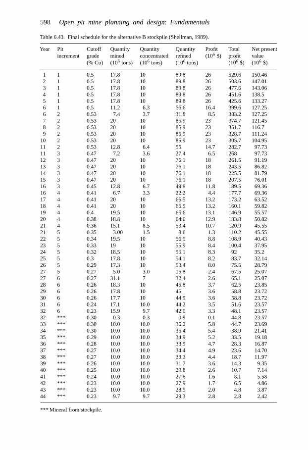
598 Open pit mine planning and design: Fundamentals
Table 6.43. Final schedule for the alternative B stockpile (Shellman, 1989).
Year Pit Cutoff Quantity Quantity Quantity Profit Total Net presentincrement grade mined concentrated refined (106 $) profit value
(% Cu) (106 tons) (106 tons) (106 tons) (106 $) (106 $)
1 1 0.5 17.8 10 89.8 26 529.6 150.462 1 0.5 17.8 10 89.8 26 503.6 147.013 1 0.5 17.8 10 89.8 26 477.6 143.064 1 0.5 17.8 10 89.8 26 451.6 138.55 1 0.5 17.8 10 89.8 26 425.6 133.276 1 0.5 11.2 6.3 56.6 16.4 399.6 127.256 2 0.53 7.4 3.7 31.8 8.5 383.2 127.257 2 0.53 20 10 85.9 23 374.7 121.458 2 0.53 20 10 85.9 23 351.7 116.79 2 0.53 20 10 85.9 23 328.7 111.24
10 2 0.53 20 10 85.9 23 305.7 104.9511 2 0.53 12.8 6.4 55 14.7 282.7 97.7311 3 0.47 7.2 3.6 27.4 6.5 268 97.7312 3 0.47 20 10 76.1 18 261.5 91.1913 3 0.47 20 10 76.1 18 243.5 86.8214 3 0.47 20 10 76.1 18 225.5 81.7915 3 0.47 20 10 76.1 18 207.5 76.0116 3 0.45 12.8 6.7 49.8 11.8 189.5 69.3616 4 0.41 6.7 3.3 22.2 4.4 177.7 69.3617 4 0.41 20 10 66.5 13.2 173.2 63.5218 4 0.41 20 10 66.5 13.2 160.1 59.8219 4 0.4 19.5 10 65.6 13.1 146.9 55.5720 4 0.38 18.8 10 64.6 12.9 133.8 50.8221 4 0.36 15.1 8.5 53.4 10.7 120.9 45.5521 5 0.35 3.00 1.5 8.6 1.3 110.2 45.5522 5 0.34 19.5 10 56.5 8.8 108.9 40.4323 5 0.33 19 10 55.9 8.4 100.4 37.9524 5 0.32 18.5 10 55.1 8.3 92 35.225 5 0.3 17.8 10 54.1 8.2 83.7 32.1426 5 0.29 17.3 10 53.4 8.0 75.5 28.7927 5 0.27 5.0 3.0 15.8 2.4 67.5 25.0727 6 0.27 31.1 7 32.4 2.6 65.1 25.0728 6 0.26 18.3 10 45.8 3.7 62.5 23.8529 6 0.26 17.8 10 45 3.6 58.8 23.7230 6 0.26 17.7 10 44.9 3.6 58.8 23.7231 6 0.24 17.1 10.0 44.2 3.5 51.6 23.5732 6 0.23 15.9 9.7 42.0 3.3 48.1 23.5732 *** 0.30 0.3 0.3 0.9 0.1 44.8 23.5733 *** 0.30 10.0 10.0 36.2 5.8 44.7 23.6934 *** 0.30 10.0 10.0 35.4 5.4 38.9 21.4135 *** 0.29 10.0 10.0 34.9 5.2 33.5 19.1836 *** 0.28 10.0 10.0 33.9 4.7 28.3 16.8737 *** 0.27 10.0 10.0 34.4 4.9 23.6 14.7038 *** 0.27 10.0 10.0 33.3 4.4 18.7 11.9739 *** 0.26 10.0 10.0 31.7 3.6 14.3 9.3540 *** 0.25 10.0 10.0 29.8 2.6 10.7 7.1441 *** 0.24 10.0 10.0 27.6 1.6 8.1 5.5842 *** 0.23 10.0 10.0 27.9 1.7 6.5 4.8643 *** 0.23 10.0 10.0 28.5 2.0 4.8 3.8744 *** 0.23 9.7 9.7 29.3 2.8 2.8 2.42
*** Mineral from stockpile.

Production planning 599
Figure 6.28. Simple sequencing example.
Figure 6.29. Mining sequence –scenario 1.
Scenario 1. Removal of waste followed by ore miningFor operational simplicity it would be best if all of the waste could be stripped (removed)first followed later by ore mining. This is shown in Figure 6.29.
The net present value for this sequence assuming an interest rate of 10% is
NPV = −$5
(1.10)1+ −$5
(1.10)2+ $10
(1.10)3+ $10
(1.10)4
= −$4.55 − $4.13 + $7.51 + $6.83 = $5.66
Scenario 2. One year of pre-stripping followed by both ore (3 blocks/year) and waste(2 blocks/year) miningThis alternative would require mining 5 blocks of waste in year 1. In years 2 and 3 threeblocks of ore would be mined for every two blocks of waste. The final year would have1 block of waste and 4 blocks of ore. The sequencing is shown in Figure 6.30.
The net present value is now
NPV = −$5
(1.10)1+ $4
(1.10)2+ $4
(1.10)3+ $7
(1.10)4
= −$4.54 + $3.31 + $3.01 + $4.78 = $6.56
Scenario 3. Mining of waste is maintained one block ahead of oreComparing scenarios 1 and 2, there was an improvement in the net present value when thetime lag between stripping and mining was shortened. In this third scenario, the stripping
pjw
stk|
4020
64|1
4356
0357
7

600 Open pit mine planning and design: Fundamentals
Figure 6.30. Mining sequence –scenario 2.
Figure 6.31. Mining sequence –scenario 3.
will be kept only one block ahead of ore mining, to make the time lag even shorter. This isshown in Figure 6.31.
The net present value is
NPV = $1
(1.10)1+ $2.50
(1.10)2+ $2.50
(1.10)3+ $4
(1.10)4
= $0.91 + $2.07 + $1.88 + $2.73 = $7.59

Production planning 601
Figure 6.32. Mining sequence –scenario 4.
Scenario 4. Stripping is maintained one half block ahead of ore miningA major improvement in the NPV was observed between scenarios 2 and 3. To explore thisfurther, consider the situation when the stripping lead is cut to one-half block (Figure 6.32).
The NPV is
NPV = $1.75
(1.10)1+ $2.50
(1.10)2+ $2.50
(1.10)3+ $3.25
(1.10)4
= $1.59 + $2.07 + $1.88 + $2.22 = $7.76
This would appear to be the most favorable alternative of the four scenarios. However,suppose that in reducing the stripping lead it is found that the operating costs for both oreand waste increase by $0.05/block, perhaps through lack of sufficient working space orthrough neglect of drilling precision because of time pressures. Hence the cost for wasteremoval increases to $1.05/block and the net ore revenue drops to $1.95/block.
The actual NPV is
NPV = $1.50
(1.10)1+ $2.25
(1.10)2+ $2.25
(1.10)3+ $3.00
(1.10)4
= $1.36 + $1.86 + $1.69 + $2.05 + $6.96
In this case scenario 3 remains the most attractive.
Scenario 5. Mining rate doubledIt has been suggested that with the purchase of more equipment, the mining rate could beincreased to 10 blocks per year. There would be an increase in the equipment ownershipcosts to be charged against both ore and waste however. The resulting values are:
Waste cost = $1.10/block
Ore revenue = $1.90/block
Stripping will be kept one block ahead of ore mining as in scenario 3.
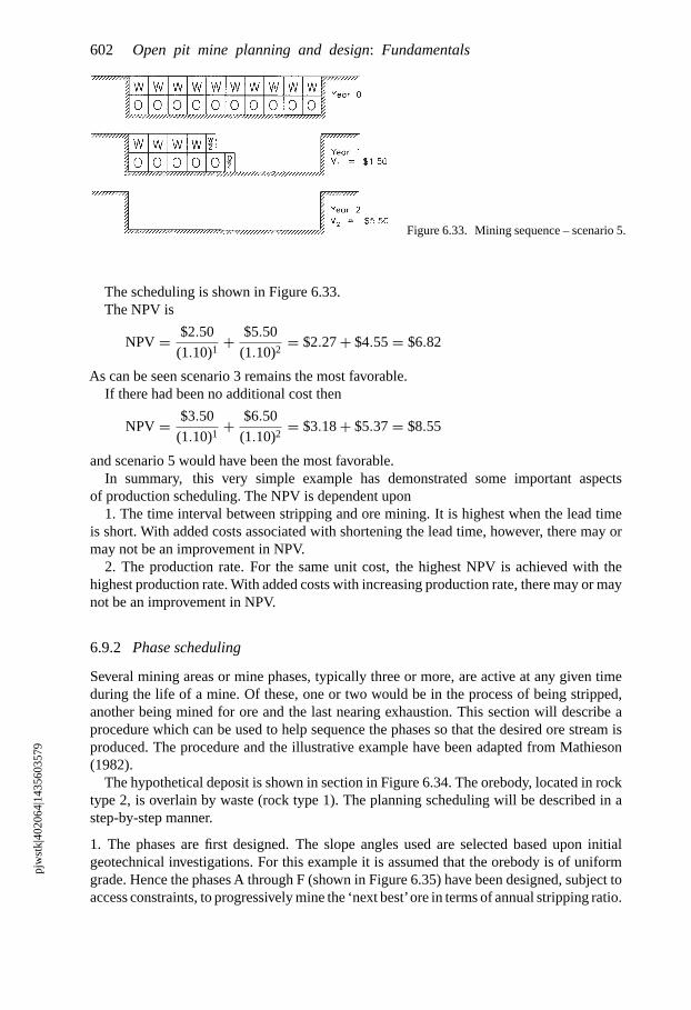
602 Open pit mine planning and design: Fundamentals
Figure 6.33. Mining sequence – scenario 5.
The scheduling is shown in Figure 6.33.The NPV is
NPV = $2.50
(1.10)1+ $5.50
(1.10)2= $2.27 + $4.55 = $6.82
As can be seen scenario 3 remains the most favorable.If there had been no additional cost then
NPV = $3.50
(1.10)1+ $6.50
(1.10)2= $3.18 + $5.37 = $8.55
and scenario 5 would have been the most favorable.In summary, this very simple example has demonstrated some important aspects
of production scheduling. The NPV is dependent upon1. The time interval between stripping and ore mining. It is highest when the lead time
is short. With added costs associated with shortening the lead time, however, there may ormay not be an improvement in NPV.
2. The production rate. For the same unit cost, the highest NPV is achieved with thehighest production rate. With added costs with increasing production rate, there may or maynot be an improvement in NPV.
6.9.2 Phase scheduling
Several mining areas or mine phases, typically three or more, are active at any given timeduring the life of a mine. Of these, one or two would be in the process of being stripped,another being mined for ore and the last nearing exhaustion. This section will describe aprocedure which can be used to help sequence the phases so that the desired ore stream isproduced. The procedure and the illustrative example have been adapted from Mathieson(1982).
The hypothetical deposit is shown in section in Figure 6.34. The orebody, located in rocktype 2, is overlain by waste (rock type 1). The planning scheduling will be described in astep-by-step manner.
1. The phases are first designed. The slope angles used are selected based upon initialgeotechnical investigations. For this example it is assumed that the orebody is of uniformgrade. Hence the phases A through F (shown in Figure 6.35) have been designed, subject toaccess constraints, to progressively mine the ‘next best’ore in terms of annual stripping ratio.
pjw
stk|
4020
64|1
4356
0357
9

Production planning 603
West East
Rock Type 2
Ore Body
Rock Type 1
Figure 6.34. Hypothetical deposit for the sequencing study (Mathieson, 1982).
West East
RockType 1
RockType 2
Ore Ultimate Pit Limit
Design Phase Limits
FC B A D E
Figure 6.35. Development scheme for the hypothetical deposit (Mathieson, 1982).
pjw
stk|
4020
64|1
4356
0357
4

604 Open pit mine planning and design: Fundamentals
Table 6.44. Tonnage-grade inventory by phase and bench (Mathieson, 1982).
Thousands of tons
Bench ‘A’ phase ‘B’ phase ‘C’ phase
Waste Ore Waste Ore Waste Ore
5100 15005050 32005000 5000 200 4004950 3800 1800 15004900 1500 2000 18004850 400 1000 1500 22004800 300 900 400 900 16004750 200 800 300 900 300 10004700 200 700 500 20004650 100 600 800 22004600 300 17004550 100 700
15,900 2700 6500 3100 9500 7600
Table 6.45. Summary of phase quantities (Mathieson, 1982).
Thousands of tons
Phase Waste above Waste on Ore Ore life* Cumulative orefirst ore bench ore benches (yrs) life* (yrs)
A 15,000 900 2700 1.08 1.08B 5500 1000 3100 1.24 2.32C 7500 2000 7600 3.04 5.36D 12,800 3800 12,500 5.00 10.36E 18,200 4900 15,100 6.04 16.40F 22,000 4500 13,000 5.20 21.60
Total 81,000 17,100 54,000 21.60
*Assuming an annual milling rate of 2,500,000 tons.
2. The ore-waste tonnage inventory by bench and phase is determined. The detailed resultsfrom the first 3 phases are given in Table 6.44. At this point the mining engineer would‘mine’ the ore on each successive bench gradually stepping, in order, through the phasesto meet the required annual mill production. Such an ore schedule would typically be doneusing a hand calculator or an interactive desk top computer program. Each phase would havea different ore life since they were defined on operating rather than schedule constraints.The first trials would be based upon a fixed cutoff grade.
3. For this simple example the overall phase quantities given in Table 6.45 will be used.Normally those broken down bench-by-bench (Table 6.44) would be considered.
4. These phases will be mined in sequence and no inter-phase blending will be consideredin this simple schedule. Each phase contains a tonnage of ore which must be exposed ordeveloped prior to the exhaustion of ore from the previous phase. A 2.5 million ton per yearmilling rate is assumed. This is divided into the ore tons available in each phase to determine

Production planning 605
(a) Schedule For Developed Ore
(b) Stripping Schedule
20.0D
EV
ELO
PE
D O
RE
(106
tons
)C
UM
ULA
TIV
E S
TR
IPP
ING
(106
tons
)
15.0
10.0
5.0
�10 �5 5
TIME (YEARS)
TIME (YEARS)
10 15 20 25
4.5
4.918.2
3.812.8
2.07.5
1.0
0.915A
5.5
22.0
0
�10 �5 5 10 15 20 250
20
40
60
80
100
B
C
D
E
F
Figure 6.36. Developed ore and stripping schedules.
phase life. A saw-tooth plot of available ore versus time is made such as is shown in Figure6.36a. This illustrates the availability and depletion of ore from the various phases.
5. The planner is now able to define the points in time at which the waste stripping must becompleted for any given phase in order to sustain the ore supply. For phase A ore productionto commence, the 15 million tons of waste lying above the first bench must have first beenremoved. During the mining of Phase A there is an additional 900,000 tons of internal wasteassumed to be evenly distributed and ‘locked-up’with the ore. In order for the phase B ore tobe available, 21,400,000 tons of waste must be removed. The cumulative waste tons versustime plot is shown in Figure 6.36b. The vertical steps in the plot correspond to the respective

Open pit mine planning and design: Fundamentals
CU
MU
LAT
IVE
ST
RIP
PIN
G(1
06 to
ns)
TIME (YEARS)
PRO
POSE
D C
UM
ULA
TIVE
STR
IPPI
NG
SC
HED
ULE
�10 �5 5 10 15 20 250
A
B
C
D
E
F
20
40
60
80
100
Figure 6.37. Proposed cumulative stripping schedule for the example orebody.
overburden stripping quantities above the first ore bench of each phase. The latter segmentsrepresent the progressive mining of internal waste.
6. The next step is to arrive at a ‘smoothed’ stripping schedule which exceeds the minimum.A possible schedule is shown as the straight line superimposed on Figure 6.37. It consistsof a 4 year pre-production period totalling 20 million tons followed by a constant strippingrate of 5 million tons per year through year 15. Beyond this only the internal waste of phaseF remains.
The detailed preproduction stripping schedule is shown in Figure 6.38. It consists of 2.5million tons during the first year when the crews are being trained and equipment is beingdelivered. During years 2 and 3 the stripping rate is 5 million tons/year. Finally in year 4the rate is increased to the total material rate (ore plus waste) which will be sustained nearlythroughout the remaining life. It can be seen from the figure that the required stripping iscompleted prior to the required time by various amounts.
Phase Early completion (months)
A 8B 9C 4D 5E 9F 16
7. The initial curve of developed ore versus time is now adjusted to reflect the early comple-tion of the stripping. This construction is shown in Figure 6.39. The cumulative strippingand developed ore curves are used. For phase B one moves horizontally at the required
606

Production planning
10
20
CU
MU
LAT
IVE
ST
RIP
PIN
G(1
06 to
ns)
The Slopes Shown arein 106 tons/year
Start of Production
�5 �3 �1 0 1
TIME (YEARS)
2.5
5.0
5.0
5.0
5.0
7.5
Figure 6.38. Preproduction stripping schedule.
00 1 3 4
0
20
40
�1�3�5 1 32 4 5 6 7 8
5.0
10.0
15.0
DE
VE
LOP
ED
OR
E(1
06 to
ns)
CU
MU
LAT
IVE
ST
RIP
PIN
G(1
06 to
ns)
TIME (YEARS)
Increased Availabilityof Developed OreDue To Early Completionof Stripping
A B
A
B
C
D
C
D
Figure 6.39. Construction showing modification of oreavailability.
cumulative stripping level to the actual stripping curve. Then one proceeds vertically to thedeveloped ore curve. As can be seen there are approximately 2 million tons of ore fromphase A remaining. Due to the early development of phase B, an additional 3.1 milliontons of ore become available. The construction is simply to extend the slanted portion of
607pj
wst
k|40
2064
|143
5603
594

Open pit mine planning and design: Fundamentals
the phase B ore reserve upward until it meets the vertical line from the stripping graph.This process is repeated for phases C through F. For phase A, the ore in the phase simplybecomes available earlier. The cross hatched areas indicate contingency ore available in thecase that the stripping schedule falls behind. The modified developed ore curve representsthe predicted inventory balance with time. A further acceleration of stripping is sometimesdone in the trial scheduling process to guard against possible surprises in mineable reserves.This can help to avoid:
– an unexpected crash stripping program,– a forced reduction in mill feed,– a temporary lowering of the cutoff grade to sustain planned concentrate production.
8. With this thorough understanding of the orebody and its development options, the pitplanner presents his/her findings to management.
9. Final mine plan period maps are drawn up to test the viability of the plan. Some refinementsin the ramping and phasing strategy, etc., may be needed but major changes are unlikely.
10. To this point, a series of logical pit development phases have been defined based on the‘next best’ profitable ore and a fixed cutoff. The plan can now be fine tuned. Alternative oreand waste schedules based on variable production rate and cutoff grade strategies can bedeveloped using the computed tonnage – grade inventories within each successive phase.Such schedules can then be compared economically through standard internal ROR analy-sis. A visual comparison can be achieved by plotting cumulative operating cash flow withtime.
11. Once a ‘final’production schedule has been decided upon, the planner generates a seriesof period end plans. These might be for example:
(a) end of preproduction,(b) years 1–5 in yearly increments,(c) years 10, 15, etc.
These plans would be based on both the phase designs and the paper schedules. They wouldconstitute a vital test on the mineability of the proposed plan. Shovel and drill deploymentand any internal temporary ramping would also be considered in detail.
6.9.3 Block sequencing using set dynamic programming
IntroductionIn 1974, Roman (1974) described an algorithm for determining the optimum miningsequence and pit limits patterned after one originally presented by Lerchs & Grossmann(1965). The process will be demonstrated through the use of a 2-dimensional example.Figure 6.40 is a schematic representation of a slice through a block model.
An index number representing the column and row position for each block is assigned.The first step in the process is to convert the grade block model into an economic blockmodel. To assign the appropriate costs and revenues a decision must be made at this pointregarding the destination of each block. Three possibilities might be:
– mill,– leach dump, and– waste dump.
608

Production planning
Figure 6.40. Schematic of the ore deposit showing block numbers and grades (Roman, 1974).
Figure 6.41. Schematic of the ore deposit showing block numbers and block values (Roman, 1974).
The net block value is determined by subtracting the mining and processing costs fromthe revenues. The mining costs are for the block alone and do not include stripping costs.Figure 6.41 shows the resulting economic block model. At this point a constraint relatingto the final pit slope is introduced.
Constraint 1: The pit wall slope may not exceed 1:1 at any point.Applying the floating cone procedure introduced in the previous chapter one would arriveat the final pit shown in Figure 6.48. This same result will be achieved using the techniquedescribed in this section. The problem is to determine the sequence in which the blocksshould be mined so that the net present value for the section is a maximum.
609

Open pit mine planning and design: Fundamentals
Figure 6.42. Schematic of the ore deposit with the final pit limits as determined using the floating conesuperimposed.
The optimum sequence. To begin the sequence optimizing process, the economic blockmodel is scanned to determine the maximum outline which the future pit could assume.Obviously all of the positive blocks on the section must be included and the pit limit slopesobeyed. The objective is to identify the location of the last block which might be mined.In this example, the last block has been selected as the bottom vertice of the invertedtriangle containing all blocks of positive value. This triangle shown in Figure 6.43 has beenconstructed in accordance with constraint 1. An alternative procedure would be to selecta hypothetical block (a block that does not exist) lying on or below the lowest level ofpositive blocks. To simplify the discussion, the triangle approach has been used. There are36 blocks included within the triangle. If each block corresponds to a unit time period (ofunspecified length), 36 time periods are required to mine all of the blocks. Block (7,6) asseen in Figure 6.44 is the last one to be mined. It is mined in period 36. In order to mineblock (7,6) one must first mine blocks (6,5), (7,5) and (8,5). At this point a second constraint,one regarding sequencing, will be introduced.
Constraint 2: Each mining level may be entered at only one point.With this constraint in place there are only two sequencing options for the mining of blocksin time periods 35 and 36:Option 1. Mine block (6,5) followed by block (7,6) (Figure 6.45a).Option 2. Mine block (8,5) followed by block (7,6) (Figure 6.45b).The third option (shown in Figure 6.45c) of mining block (7,5) in period 35 means thatboth blocks (8,5) and (6,5) had been mined earlier. This requires that two separate entriesbe made on level 5 thus violating constraint 2. Hence this is not an option.
In time period 34 there are several choices for the block to be mined depending upon theblock mined in period 35. If the last two blocks mined are (6,5) and (7,6) then the possiblesequences for the last 3 periods are
(1) (7, 5) → (6, 5) → (7, 6)
(2) (8, 5) → (6, 5) → (7, 6)
(3) (5, 4) → (6, 5) → (7, 6)
610

Production planning
Figure 6.43. Schematic of the ore deposit showing the triangle containing the maximum pit superimposed(Roman, 1974).
Figure 6.44. Blocks which must be removed prior to mining block 36.
On the other hand if blocks (8,5) and (7,6) are mined last then the possible sequences are:
(4) (6, 5) → (8, 5) → (7, 6)
(5) (7, 5) → (8, 5) → (7, 6)
(6) (9, 4) → (8, 5) → (7, 6)
These 6 possibilities are shown in Figure 6.46.Sequences 2 and 4 however involve mining the same 3 blocks in just a different order. An
economic evaluation is performed to determine the most attractive of the two alternatives.
611

Open pit mine planning and design: Fundamentals
Figure 6.45. Possible sequences for mining blocks 35 and 36.
The least attractive is dropped from further consideration. Choosing an interest rate of 10%and discounting to the beginning of time period 34 one finds:
Sequence 2: (8, 5) → (6, 5) → (7, 6)
NPV2 = $3
(1.1)1− $5
(1.1)2− $6
(1.1)3= −$5.91
612

Production planning
Figure 6.46. Possible sequences for mining blocks 34, 35, and 36.
Sequence 4: (6, 5) → (8, 5) → (7, 6)
NPV2 = −$5
(1.1)1+ $3
(1.1)2− $6
(1.1)3= −$6.57
613

Open pit mine planning and design: Fundamentals
Figure 6.46. (Continued).
614
Production planning
Sequence 4 is the least attractive of the two and is dropped. The five block combinationsfor periods 34 through 36 which must be included when sequencing the remaining 33periods are:
Sequence Mining order
1 (7,5) → (6,5) → (7,6)2 (8,5) → (6,5) → (7,6)3 (5,4) → (6,5) → (7,6)4 (7,5) → (8,5) → (7,6)5 (9,4) → (8,5) → (7,6)
The remaining choices for sequencing the final four blocks after eliminating duplicatecombinations of blocks by the present value analysis are:
Sequence Mining order
1 (8,5) → (7,5) → (6,5) → (7,6)2 (9,4) → (8,5) → (6,5) → (7,6)3 (7,5) → (5,4) → (6,5) → (7,6)4 (8,5) → (5,4) → (6,5) → (7,6)5 (4,3) → (5,4) → (6,5) → (7,6)6 (9,4) → (7,5) → (8,5) → (7,6)7 (10,3) → (9,4) → (8,5) → (7,6)
This process is continued until all 36 blocks have been included. In this final stagethe various sequences will just be permutations of the same combination. Consequentlythe optimum sequence can be determined through a present value calculation. Fig-ure 6.47 shows the section with the 36 blocks numbered in the order that they are to beremoved.
Determination of the optimum pitOnce the optimum sequence has been found, the pit outline can be developed. The procedurefor determining which of the 36 blocks in the optimum sequence are actually to be minedis as follows:
1) Identify the last block in the optimum sequence with a positive value. Drop all blocksafter this one.
2) Examine the remaining sequence of blocks and identify the latest negative blockscheduled for mining. If there are a number of negative blocks in a row select the earliest inthe row. Determine the present worth for the sequence extending from identified negativeblock to the end.
3) If the present value is negative, drop all these blocks from the optimum sequence andrepeat step 2. If the subsequence has a positive present value, replace the subsequence byan equivalent block value at the end of the sequence.
4) Repeat steps 2 and 3 until the first mined block is included in the subsequence. Thefinal present value is that of the optimum pit.
Applying these rules to the example problem, it is seen that blocks 31 through 36, whichare all negative, are dropped by inspection. Continuing along the sequence it is seen that twoadjacent blocks (13,1) and (4,2) corresponding to mining periods 26 and 27 respectively,are negative. The net present value for this subsequence (blocks 26 to 30) discounted to the
615

Open pit mine planning and design: Fundamentals
Figure 6.47. Schematic of the deposit showing the optimum block mining sequence (Roman, 1974).
beginning of period 26 is
NPV = −$1
(1.1)1− $2
(1.1)2+ $2
(1.1)3+ $1
(1.1)4+ $2
(1.1)5
= $0.87
Since it is positive, this subsequence, referred to as subsequence SS1 is retained. The nextswitch between negative and positive blocks occurs after block 21. The net present valuefor the subsequence SS2 through to the beginning of period 21 is
NPV = −$1
(1.1)1− $2
(1.1)2+ $1
(1.1)3+ $2
(1.1)4+ $3
(1.1)5+ $0.87
(1.1)6
= $1.91
616

Production planning
Figure 6.48. The final pit outline and optimum mining sequence (Roman, 1974).
It is positive and hence retained. This process of calculating net present value is continueduntil the first block to be mined is included. The final pit is shown in Figure 6.48. The overallNPV for the pit on this section is
NPV (overall) = $12.60
Simply summing the values of the blocks included within the outlined yield
Sum = $34
This would be the result if the pit could be mined instantaneously at time zero.
617

Open pit mine planning and design: Fundamentals
Figure 6.49. Hypothetical deposit showing block values and maximum pit limits (Roman, 1974).
Figure 6.50. Mining sequence and pit limit for an interest rate of 5% (Roman, 1974).
Time value of money inf luenceIn the previous example, a 10% discount rate was applied in arriving at the optimum sequenceand pit. The question arises as to the influence this rate has both on the sequence and the finalpit. Figure 6.49 shows the section to be used with the maximum pit superimposed. Usingthe techniques and constraints previously described the pits corresponding to the use of 5%,10%, 20%, and 50% discount rates are shown in Figures 6.50 through 6.53 respectively. Ascan be seen, a definite effect is observed. At first glance it would appear that the reductionin pit size between discount rates of 5% and 10% is incorrect since the strip of blocks
(12, 1) → (11, 2) → (10, 3) → (9, 4) → (8, 5) → (7, 6)
when summed has a positive value (+1). However when taking sequencing into account thediscounted value of this strip (at a rate of 10%) is
NPV = $3.5
(1.1)36− $3.0
(1.1)35− $2.0
(1.1)34− $1
(1.1)33− $1.5
(1.1)32− $1.0
(1.1)31
= −$0.025
For higher discount rates this sub-sequence is even more negative.
618

Production planning
Figure 6.51. Mining sequence and pit limit for an interest rate of 10% (Roman, 1974).
Figure 6.52. Mining sequence and pit limit for an interest rate of 20% (Roman, 1974).
Figure 6.53. Mining sequence and pit limit for an interest rate of 50% (Roman, 1974).
The rate to be used depends upon a number of factors, the principal one being that ofcompany policy. In the early stages of a property, a high rate of return is generally desiredin order to repay the investment as quickly as possible. Later when the investment has beenrepaid, another value may apply. Thus the procedure outlined is not intended to be usedjust once in the life of a property and the derived sequence to be followed without change.
619
Open pit mine planning and design: Fundamentals
Rather with changing conditions, it can be rerun on the blocks remaining at any given timeand a new optimum sequence developed.
SummaryThe described sequencing procedure is quite simple. Although the examples were2-dimensional in nature, programs containing the algorithm have been written for the true3-dimensional pit problem. Changes in constraints on the mining sequence can be incor-porated relatively easily. In theory, the size of problem which can be handled is unlimited.However as was seen in the 2-dimensional hand example, the number of sequences to beconsidered increases rapidly as the number of blocks contained in the deposit increases.A relatively large and fast computer is required to perform the calculations for even a smalldeposit. A deposit for which ore characteristics fluctuate radically and continually alongany direction will require more computer time and storage to evaluate. On the other hand,adding constraints on the mining sequence tends to simplify the problem. If in the problemof sequencing the 36 blocks constraint 2 is dropped, the required computer time increasesby a factor of 30 and the storage by 20 times.
Rather than attempting to provide an overall optimum sequence for an entire depositconsisting of many thousands of blocks, the mine plan may be first broken down into aseries of phases. The sequencing procedure can then be applied to each of the phases inturn. In this way a series of sub-optimizations is realized. Being sub-optimizations, due careshould be taken in putting these phases together, but it is possible in practice to build up agood mine plan in this way.
6.9.4 Some scheduling examples
Dagdelen (1985) has applied the Lagrangian parametrization technique for optimum openpit mine production scheduling. A full discussion of the procedure is beyond the scope ofthis textbook. An ultimate pit limit contour is first obtained using Lerchs-Grossmann’s 3-Dalgorithm. A series of constraints such as: (a) mining capacity, (b) milling capacity, (c) millfeed grade, (d) geometric (i.e. slope limitation), are then introduced.
The program searches through the set of candidate blocks and selects those yielding amaximum net present value for the deposit while meeting the constraints. The results ofapplying this procedure to a small high grade copper deposit are included here to demonstratethe effect of changing constraints.
The grade block model (25 × 20 blocks) for benches 1 through 6 of this deposit is shownin Figure 6.54. The pit limits obtained using a 45 degree slope constraint have been superim-posed. Each of the blocks has plan dimensions 100 ft × 100 ft and the block (bench) heightis 45 ft. The assumptions made in the development of the economic block model are givenin Table 6.46. The level by level statistics of reserves in the ultimate pit limit contour aregiven in Table 6.47. The tonnage factor for both ore and waste is 12.0 ft3/ton, hence thereare 37,500 tons of material per block. The overall material in the pit consists of
Material Blocks Tons Grade
Waste 505 18,937,500 0Ore 63 2,362,500 3.68% CuTotal 568 21,300,300 NA
If all the material in the pit could be mined instantaneously then the net value (revenues-costs) would be about $57,632,000. It will be assumed to be mined over a 3 year period
620

Production planning
Figure 6.54. Grade block model with final pit limits superimposed. The number 1 denotes waste withgrade 0 (Dagdalen, 1985).
instead. A discounting rate of 12.5% will be assumed. The precedence (order of mining)and slope constraints which apply are respectively
– In order to remove a given block, overlying blocks in the cone of influence must beremoved first.
– Pit slopes may not exceed the given maximum values (45◦ in this case).– The bench faces are considered to be vertical.
621

Open pit mine planning and design: Fundamentals
Figure 6.54. (Continued).
Constraint example 1The first schedule will be made subject to the following ore mining (milling) capacityconstraint:
1. Mine 19 ore blocks in period 1.2. Mine 21 ore blocks in period 2.3. Mine 23 ore blocks in period 3.
The problem is to schedule the operation such that the above restrictions are not violatedand, at the same time, the total discounted profits before tax are maximized. The resulting
622

Production planning
Figure 6.54. (Continued).
Table 6.46. Values used in the economic block model calculation(Dagdalen, 1985).
Price of copper $0.80 per lbMining costs $0.85 per ton of materialMilling costs $2.20 per ton of oreSmelting, refining and marketing $0.25 per lb of CuG&A $0.15 per ton of oreOverall metal recovery 85%
623

Open pit mine planning and design: Fundamentals
Table 6.47. Summary of the reserves within the ultimate pit limits bylevel (Dagdalen, 1985).
Number of Ave. Number ofBench ore blocks grade waste blocks
1 1 6.10 1962 9 2.88 1343 10 3.84 954 13 4.26 555 16 3.49 256 14 3.57 0
Total 63 3.68 505
schedules are shown in Figure 6.55 and in Table 6.48. In Figure 6.55, the numbers indicatethe period in which each block is scheduled to be mined.
The average grade of the ore mined is 3.7% Cu in the first year, goes up to 4.4% Cu inthe second year and decreases to 3.0% Cu in year 3 (Table 6.49).
According to the schedule, very little stripping is required in year 1; the amount ofstripping is more than doubled in year 2; and most of the stripping is done in year 3. Nocost adjustments have been made to reflect this schedule. The net present value of thisschedule is
NPV = $20, 352, 206
1.125+ $25, 341, 619
(1.125)2+ $11, 857, 556
(1.125)3
= $18, 090, 850 + $20, 023, 008 + $8, 327, 941
= $46, 441, 800
Imposing yearly ore tonnage constraints on the system together with discounting reducedthe net present value by $11,190,225.
Constraint example 2For this example, an additional restriction on mill feed grade is imposed together with theore mining capacity constraints of the previous example; specifically:
1. Mine 19 ore blocks averaging 3.7% Cu in year 1.2. Mine 21 ore blocks averaging 3.7% Cu in year 2.3. Mine 23 ore blocks averaging 3.7% Cu in year 3.
As indicated in the discussion of the ultimate pit reserves, the average grade of the totalreserve within the ultimate pit contour was 3.68% Cu. Hence, this new restriction is to forcethe operation to mine as close to this average grade as possible.
The optimum solution to the above mining system is depicted in Figure 6.56. The numberson the different benches indicate the years in which the block will be mined.
The summary statistics by bench and year are given in Table 6.50.All of the constraints are satisfied except for the average grade requirement in year 2.In year 2 the average grade is 3.6% as compared to the required 3.7%. The reason for this
is a lack of available blocks. Table 6.51 summarizes the results. The NPV for this schedule,$45,929,335, is slightly less than that obtained in the previous example.
624

Production planning
Figure 6.55. Proposed mining sequence for years 1, 2 and 3 under constraint set 1 (Dagdalen, 1985).
This reduction is caused by blending some of the low grade material with high grade inperiod 2.
These example studies can be expanded to include other conditions to determine theeffects and costs of different constraints on the system.
625

Open pit mine planning and design: Fundamentals
Figure 6.55. (Continued).
6.10 PUSH BACK DESIGN
6.10.1 Introduction
The first step in the practical planning process is to break the overall pit reserve into moremanageable planning units. These units are commonly called sequences, expansions, phases,
626

Production planning
Figure 6.55. (Continued).
working pits, slices or push backs. In the beginning quite coarse divisions covering periodsof several years may be used. They are a preliminary attempt to relate
the geometry of miningto
the geometry of the ore distribution.
627pj
wst
k|40
2064
|143
5603
591

Open pit mine planning and design: Fundamentals
Table 6.48. Level by level statistics for the optimum schedule under constraint set 1 (Dagdalen, 1985).
Year 1 Year 2 Year 3
Bench Ore Ave. Waste Ore Ave. Waste Ore Ave. Wasteblocks Grade blocks blocks grade blocks blocks grade blocks
1 1 6.10 42 0 0 50 0 0 1042 9 2.88 15 0 0 44 0 0 753 9 4.20 0 1 0.6 32 0 0 634 0 0 0 11 4.56 14 2 2.60 415 0 0 0 9 4.60 0 7 2.07 256 0 0 0 0 0 0 14 3.57 0
Total 19 3.67 57 21 4.39 140 23 3.03 308
Table 6.49. Production summary under constraint set 1 (Dagdalen, 1985).
Year Ore grade Ore Tonnage Total SR(% Cu) waste
1 3.67 712,500 2,137,500 2,850,000 3.02 4.39 787,500 5,250,000 6,037,500 6.73 3.03 862,500 11,550,000 12,412,500 13.4
Total 2,362,500 18,937,500 21,300,000 8.0
Phase planning should commence with mining that portion of the orebody which will yieldthe maximum cash flow. Succeeding phases are ordered with respect to their cash flowcontribution. Eventually the ultimate pit limits are reached.
By studying the ore grade distribution (particularly as depicted on bench plans) andthe topography the mining engineer can, in most cases, arrive at a logical pit developmentstrategy in a relatively short time. Figure 6.57 shows a two dimensional representation of thephases used to extract an ore reserve (Mathieson, 1982). The extraction sequence proceedsfrom that phase having the highest average profit ratio (APR) to the lowest. In this case theyproceed in alphabetical order A to G.
Profit ratio = Revenue
All costs
The incremental profit ratio, computed at the final pit boundary is 1.A basic overview of the steps involved in phase planning (Mathieson, 1982) are indicated
below. These will be expanded upon in the succeeding sections.
1. Before design work is initiated some preliminary judgements must be made regarding– the probable maximum ore and waste mining rate required in a given phase,– the size and type of equipment to be used. This determines the required minimumoperating bench width necessary,– appropriate working, interramp, and final slope angles.
2. Using the constraints given in step 1, the mining engineer then proceeds to design aseries of phases in some detail, complete with haul roads. He ensures that ramp access
628

Production planning 629
Figure 6.56. Proposed mining sequence for years 1, 2 and 3 under constraint set 2 (Dagdalen, 1985).
to each active bench is provided. The transition between phases is carefully planned. Thedesigner is not constrained by having to include a certain quantity or number of years of oresupply in each phase. The variable ore and waste quantities by phase will be subsequentlyscheduled.

630 Open pit mine planning and design: Fundamentals
Figure 6.56. (Continued).
3. Once complete, the phase designs are transferred onto the bench plans. Bench by benchtonnages and grades are evaluated. A tonnage-grade inventory for each phase of the logicallydefined pit development sequence is then available.
4. The last task is to determine annual mining schedules based on mill feed or productrequirements.

Production planning 631
Bench 6
Figure 6.56. (Continued).
It may be necessary to repeat this process several times before an adequate plan isdeveloped.
The development of phases makes it possible to determine the amount of pre-productionstripping required. Although the natural tendency is to keep the amount of such stripping

632 Open pit mine planning and design: Fundamentals
Table 6.50. Level by level statistics for the optimum schedule under constraint set 2 (Dagdalen, 1985).
Year 1 Year 2 Year 3
Bench Ore Ave. Waste Ore Ave. Waste Ore Ave. Wasteblocks Grade blocks blocks grade blocks blocks grade blocks
1 1 6.1 42 0 0 50 0 0 1042 9 2.88 15 0 0 44 0 0 753 9 4.20 0 1 0.6 31 0 0 644 0 0 0 10 4.16 13 3 4.60 425 0 0 0 10 3.34 0 6 3.73 256 0 0 0 0 0 0 14 3.57 0
Total 19 3.67 57 21 3.60 138 23 3.75 310
Table 6.51. Production summary under constraint set 2 (Dagdalen, 1985).
Year Ore grade Ore Tonnage Total SR(% Cu) waste
1 3.67 712,500 2,137,500 2,850,000 3.02 3.60 787,500 5,175,000 5,962,500 6.63 3.75 862,500 11,625,000 12,487,500 13.5
Total 2,362,500 18,937,500 21,300,000 8.0
Minimum PhaseOperating Width
E
A BC
DF
GAPR � 4.1
APR � Average Profit Ratio
IPR � Incremental Profit Ratio
APR � 3.6 APR � 1.2IPR � 1.0
APR � 3.
2
APR � 2
.8APR �
1.5
APR � 2.0
IPR �
3.0
IPR �
1.0
IPR � 1.0
Profit ratio � revenueall costs
Figure 6.57. Pit sequencing in order of decreasing value (Mathieson, 1982).
to a minimum since it appears as a major negative cash flow early in the mining process, itis important that enough work be done to (1) expose a sustaining ore supply, and (2) keepthe mine in a condition that allows it to be operated efficiently at all times. Sometimes thepreproduction work is contracted. However, in new large tonnage truck-shovel mines, the

Production planning 633
pre-production period provides an opportunity to build an organization and to gain operatingexperience.
6.10.2 The basic manual steps
This series of steps in manual push back design has been provided by Crawford (1989a).
1. Start with the ultimate pit limit design.– Develop detailed data of ore grade and stripping distributions for various cutoff grades
in zones around the designed pit circumference and in pit shell progression between thebeginning surface topography (or pit surface) and the design pit limit. These data shouldinclude locations of ore zones (these vary with cutoff) and the impact of the differencesbetween operating and ultimate pit slopes. Of particular interest should be locating high oregrade and low stripping zones on level plan maps and cross-sections.
– Manual planning methods are essentially trial and error approaches.
2. Planning goals typically comprise one or more of the following:– Maximize NPV economics.– Provide stable cash flow patterns.– Uniform ore grade, grade decline curve, or high grading. Frequently high grading is
used during the initial investment pay back period. The level(s) of ore grade will be relatedto the cutoff criteria.
– Uniform stripping ratio or classic stripping ratio curve.– Uniform total tonnage rate (ore + waste).– Uniform ore tonnage rate.– Uniform or variable rate of product output.
3. Operating design criteria for push back design:– Operating and remnant bench widths.– Slopes between operating benches and roads.– Overall operating slope.– Road widths and grades.– Bench height.
Some typical values are as follows:– Remnant bench width equal to bench height.– Push back widths normally 200–500 ft depending on size of pit and orebody
characteristics.– Minimum push back widths (single cut passes) about 80 ft for small equipment and
135–150 ft for 25–30 yd shovels and 150–200 ton trucks.– Road widths 50–80 ft depending on width of equipment. Maximum road grade 8–12
percent.
4. Laying out of one to several push backs. Evaluating whether they satisfy the goals,individually and collectively, is a more or less cut and try process. Normally a push back islaid out according to the operating criteria in plan and cross-section views. The plan viewapproach is used here. The operating criteria are expressed in geometric parameters (feet anddegrees). A useful tool is to make a scaled bench crest and toe pattern including operatingbench and road widths.

634 Open pit mine planning and design: Fundamentals
Plan View Cross Section
Push Back
Push Back Schematic
New Levelat Pit Rim
New Bench at Bottom
Current CrestFuture Crest
1
1
2
2
3
3
4
4
5
5
Figure 6.58. Push back schematic in plan and section views (Crawford, 1989a).
5. The push backs are shown on plan view maps as a progression of movements of benchlevel toes and crests from initial topography to ultimate pit limit (see Fig. 6.58). New levelsare created as the push back progresses at the pit rim and at the bottom. New bottom levelsare established on the basis of minimum level size and ore grades. Normally, new bottomlevels are encouraged by the need to hold stripping at reasonable levels. In addition to pitgeometry, ore/waste interface lines for the selected ore cutoff must be plotted.
6. Calculations of volumes of ore and waste are done using a planimeter to measure areas, andthe average grades within push backs are determined. The volumes of material to be removedfrom each bench are based on the average of the areas encompassed by the movements ofthe bench crest and toe from initial to new position by a push back, and the average benchheight for the zone covered. Ore and waste volumes are calculated separately. The averageore grade is determined by averaging the block values within the ore zones. In multiple pushbacks a push back serves as the initial location for a subsequent push back. The calculatedvalues are evaluated against the various goals for acceptability of the individual push backor series of push backs.
7. For plan view calculations, the planimeter is used to determine the areas of crest and toemovements; commonly called crest to crest and toe to toe calculations. If the pit geometryis sufficiently regular only the toe to toe calculation may be necessary. To achieve accurateresults, the calculation of volumes for new levels at the pit rim or at the bottom, alongirregular pit rim elevations, for roads, at the ultimate pit intercept and for irregular benchheights require special planimeter techniques. The key is to divide up the volumes to be

Production planning 635
Figure 6.59. The Phase I pit with haulageroad (Mathieson, 1982).
calculated into rectangular, parallelogram type solids with flat tops and bottoms and reliableaverage heights. The areas to be calculated must be closed polygons. The geometric layoutprior to calculation is critical for accurate results.All the benches and roads must be describedin the form of crests, toes, and average heights. Each bench and its related parts are calculatedseparately. Frequently, the drawing of a few cross-sections is helpful to keep the plan viewdrawing from becoming too confusing.
6.10.3 Manual push back design example
This section describes the construction procedure involved in designing a push back togetherwith the layout of the main haulage road. An initial Phase I pit (Figure 6.59) already exists(Mathieson, 1982). The following information applies:
− The bench toe lines are shown− Bench height = 45 ft− Toe-toe distance = 40 ft− Road width = 120 ft− Road grade = 10%
Careful examination of the bench plans and the sections have indicated that the push backshould involve the south and east portion of the pit. The north and northeast sections of thepit together with their portion of the haulroad will remain unchanged. The final pit designfor Phase II must conform with this current geometry. It has been decided that the width ofthe push back should be 320 ft. This is a multiple of the basic 40 ft dimension and providesthe desired
– tonnage for the phase, and– operating space.
Figure 6.60 shows the basic push back area and the region where no changes will occur. Thetoe of the bottom bench has been described by a series of straight line segments. It is notnecessary that they be straight lines but this facilitates the construction for this example. InFigure 6.61, that part of the Phase I pit involved directly in the push back has been removed.Sectors A and B will be modified for a smooth transition into the new pit. In Figure 6.62 theinitial construction lines are shown. Lines a–b and c–d are drawn at the desired push back

636 Open pit mine planning and design: Fundamentals
No Change Sector
Figure 6.60. Construction lines for the push back superimposed.
No Change
No
Cha
nge
A
B
Figure 6.61. The push back section removed. Sectors A and B are transition regions.
distance of 320 ft parallel to the existing pit bottom lines. Lines f–a and b–c which formthe pit corners are drawn at 45◦. They are parallel to the corresponding lines of the currentpit and at a distance of 320 ft. Line d–e has been drawn as shown recognizing that the pitwill become more elongated in the east-west direction on that side. In Figure 6.63 the initialattempt at a pit bottom design is shown. The transitional sectors A and B have been removed

Production planning 637
A
B
e
d
c
a bf
320�
320�
320�
Figure 6.62. The dimensions used for con-structing the new pit bottom.
Figure 6.63. The initial design for thebottom of the Phase II pit.
from the drawing. To assist in constructing the upper bench from this base pit, lines havebeen drawn at the ends of the line segments perpendicular to the segment. This is shown inFigure 6.64. From each corner a line bisecting the angle described by the two radiating linesis drawn.This is shown by the heavy lines in Figure 6.65. A series of lines spaced at 40 ft (thetoe-toe distance) are drawn parallel to those of the pit bottom. They are extended to join thoseof the existing pit (if appropriate) or to the corner lines. The drawing of the lines for the righthand side of the pit has been delayed pending the extension of the haulroad. In Figure 6.66,haulroad extension is shown. Due to the 10% grade and the 45 ft bench height, the distancebetween the adjacent road elevation lines shown is 450 ft. Figures 6.67 and 6.68 show theextension of the road down to the pit floor. In Figure 6.68 it can be seen that material in sector

638 Open pit mine planning and design: Fundamentals
a b
c
de
Figure 6.64. Construction of normalsat the segment end points.
Figure 6.65. Construction of toelines representing higher benches.
C must be mined to allow the road to daylight. A straight stretch having a length of one roadwidth (120 ft) is added (Fig. 6.69). From this point (g), three segments g–h, h–i, and i–d havebeen drawn connecting to segment d–e. This provides the trucks with smooth access to thepit bottom and facilitates future road extension as the pit is deepened.As before, the bisectinglines are drawn from the segment corners (Fig. 6.70). In Figure 6.71, the parallel bench linesare added and the lower design is completed. As can be seen in Figure 6.71, there is no access

Production planning 639
Figure 6.66. Extension of the road intothe new phase.
Figure 6.67. Extension of the roadalong the south side of the pit.
to the upper benches on the southeast side of the pit. This is corrected in Figure 6.72 by theaddition of a road. The intersection of the Phase II pit with the surface topography is alsoshown.
With a workable design completed, one can now examine the tonnages involved. This isdone on a bench by bench basis. Figure 6.73 shows the resulting bench geometry changesbetween the Phase I and Phase II pits. Figure 6.74 is the grade block model for bench 3835with the toe lines for the Phase I and II pits superimposed. The next step in the processis to determine the grade-tonnage distribution for each level. Each of the complete blocksin the block model has plan dimensions 100 ft × 100 ft. For these, since the scale used is

640 Open pit mine planning and design: Fundamentals
Figure 6.68. The road reaches the pitbottom elevation.
Figure 6.69. Final segments added tothe pit bottom.
1′′ = 200 ft, the block plan area is 0.25 in2. However, in viewing Figure 6.74 it can beseen that
– the toe lines create many partial blocks,– there are often several adjacent block with the same grade.
To save time, the contiguous blocks of the same grade are first identified. The area involvedis determined using a planimeter. The number of square inches obtained is written on thebench map (see Fig. 6.75). Next the areas of the individual whole or partial blocks are found.These values are also entered on to the map. A summary sheet such as shown in Table 6.52is prepared for the bench. The planimetered areas (in2) are converted into square feet (ft2)

Production planning 641
Figure 6.70. Construction at the seg-ment corners.
Figure 6.71. Road to pit bottom com-pleted.
using the scale factor and then into tons via the bench height (45 ft) and the tonnage factor(12.5 ft3/ton). Hence
1 in2area = 200 ft × 200 ft × 45 ft
12.5 ft3/ton= 144,000 tons
This conversion factor is applied to the areas in Table 6.52.The total area on this bench involved in phase II mining is 17.57 in2 hence the tonnage is
Tons = 17.57 in2 × 144, 000 tons/in2
= 2, 530, 080 tons

642 Open pit mine planning and design: Fundamentals
Figure 6.72. Road access to upperbenches added.
(a) Bench 3700
(b) Bench 3745
0 400 ft
0 400 ft
Area Mined in the Push Back
Figure 6.73. Area mine by bench between Phases I and II.
Sometimes grade classes are used. In Table 6.53 an interval of 0.05% Cu has beenemployed.
Expressed in this form it is quite easy to summarize the overall results from the entire pushback. Applying one or more cutoff grades, the amount of material falling in each categoryis found.

Production planning 643
(c) Bench 3790
(d) Bench 3835
0 400 ft
0 400 ft
(e) Bench 3880
0 400 ft
Figure 6.73. (Continued).
These results unfortunately may be unacceptable. For example, the overall strippingratio might be too high, the average grade too low, the tonnage too low, etc. Another pushback design must then be done in the same fashion. Eventually an acceptable plan willemerge.
pjw
stk|
4020
64|1
4356
0360
8

644 Open pit mine planning and design: Fundamentals
(f) Bench 3925
(g) Bench 3970
0 400 ft
0 400 ft
(h) Bench 4015
0 400 ft
Figure 6.73. (Continued).

Production planning 645
Figure 6.74. The final pit outline has been superimposed on the grade block model for bench 3835.
Figure 6.75. The areas are calculated.

646 Open pit mine planning and design: Fundamentals
Table 6.52. Summary tonnage-grade for the Phase II mining of bench 3835.
Grade Plan area Tons Grade Plan area Tons(% Cu) (in2) (103) (% Cu) (in2) (103)
0.28 0.15 21.6 0.63 0.04 5.80.30 0.15 21.6 0.64 0.91 131.00.31 0.24 34.6 0.65 0.16 23.00.33 0.08 11.5 0.66 0.25 36.00.35 0.25 36.0 0.67 1.22 175.70.36 0.65 93.6 0.68 0.23 33.10.38 0.06 8.6 0.70 0.56 80.60.39 0.55 79.2 0.71 0.07 10.10.40 0.27 38.9 0.74 0.25 36.00.41 0.20 28.8 0.75 1.53 220.30.42 0.30 43.2 0.76 0.53 76.30.45 0.25 36.0 0.78 0.17 24.50.46 0.01 1.4 0.80 0.25 36.00.48 1.33 191.5 0.81 0.02 2.90.49 0.70 100.8 0.82 0.50 72.00.50 0.82 118.1 0.83 0.25 36.00.53 0.21 30.2 0.86 0.25 36.00.54 0.25 36.0 0.88 0.37 53.30.55 0.04 5.8 0.89 0.44 63.40.56 1.20 172.8 0.90 0.01 1.40.58 0.20 28.8 0.91 0.07 10.10.60 0.04 5.8 0.92 0.32 46.10.61 0.21 30.2 0.93 0.37 53.30.62 0.96 138.2 0.94 0.21 30.2
Table 6.53. The data from Table 6.51 reorganized into grade intervals.
Grade interval Area (in2) Tons
0.26–0.30 0.30 43,2000.31–0.35 0.57 82,0800.36–0.40 1.53 220,3200.41–0.45 0.75 108,0000.46–0.50 2.86 411,8400.51–0.55 0.50 72,0000.56–0.60 1.44 207,3600.61–0.65 2.28 328,3200.66–0.70 2.26 325,4400.71–0.75 1.85 266,4000.76–0.80 0.42 60,4800.81–0.85 0.77 110,8800.86–0.90 1.07 154,0800.91–0.95 0.97 139,680
Total 17.57 2,530,080

Production planning 647
It is obviously possible to evaluate various push back options without going to the troubleof including the haulroads. However, a considerable amount of material is involved in lateradding such a road to the design and the results can change markedly.
6.10.4 Time period plans
Most of the pit planner’s work (Couzens, 1979) is done on plan or bench maps. These show:– topography or surface contour,– location of ore,– geologic boundaries, and– design limits.
Pit composite maps showing the shape of the mine at the end of each planning period shouldbe kept up. These enable the planner to:
– avoid conflicts between features of the plan,– provide a picture of the access at each stage of development,– illustrate the actual working-slopes, operating room and spacial relationships between
ore and waste.The transition from phase plans to time period plans should be made as soon as the phasedesigns are complete enough to set the overall pattern. The yearly plans:
– Enable definite production goals to be set in space as well as in quantities of materialto be moved.
– Allow better economic evaluations than the phase average provide.– Give a better definition of the relationship of the phases to each other as they
overlap in the complete mine operation. They show actual operating slopes and haulageroutes.
Figures 6.76, 6.77, and 6.78 show such a 3-year progression of benches in an open pitmine (Couzens, 1979).
The midbench contours have been plotted. The haulroads, stripping areas and part ofthe waste dumps are also shown. In this system the labelling of elevations is as follows(Couzens, 1979):
(a) Outside of the pit the contours are labelled with their true elevations.
(b) Inside of the pit:– The labelled elevations refer to the bench toe elevations.– The elevations of bench centerlines are one-half the bench height above the bench toe
elevation. Thus it is the flat areas between center lines that are labelled.– On ramps, the bench centerlines cross the ramp halfway between benches. The labels
are positioned at would be the actual bench elevation on the road.– For more explanation of the labelling, (see Section 4.7).
At an operating mine there will be a number of different plans covering different periods.The engineering staff is generally responsible for:
– annual ore reserve estimation,– yearly or multi-yearly plans regarding the progression of the pit, changes in haul roads,
etc.,– quarterly plans, and– monthly plans.

648 Open pit mine planning and design: Fundamentals
Figure 6.76. Bench composite for year 1 (Couzens, 1979).
The operating staff develop:– weekly plans, and– daily plans
within the longer range framework.

Production planning 649
Figure 6.77. Bench composite for year 2 (Couzens, 1979).
6.10.5 Equipment fleet requirements
Once phase plans have been developed, equipment fleet requirements can be examined(Couzens, 1979). A graph showing the total tonnage movement and waste/ore ratios can beprepared. On such a graph, the planner can see what must be done to adjust or smooth out
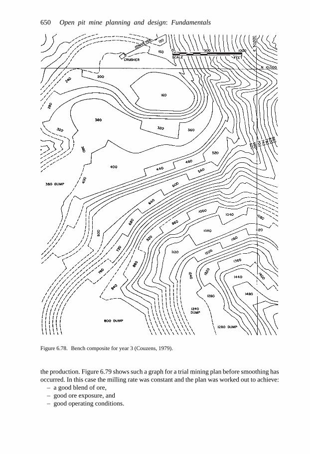
650 Open pit mine planning and design: Fundamentals
Figure 6.78. Bench composite for year 3 (Couzens, 1979).
the production. Figure 6.79 shows such a graph for a trial mining plan before smoothing hasoccurred. In this case the milling rate was constant and the plan was worked out to achieve:
– a good blend of ore,– good ore exposure, and– good operating conditions.

Production planning 651
Cumulative Ore Tonnage Scale
Production Year Scale
0 50 mm 100 mm 150 mm 200 mm 250 mm 300 mm 350 mm 400 mm 450 mm
15 mm TONINCREMENTS
35 mm TON INCREMENTS
0 1 2 3 4 5 6 7 8 9 10 11 12 13 14 15 160.0
0.5
1.0
1.5
2.5
2.0
Str
ippi
ng R
atio
(Cumulative Ratiosin Parentheses)
2.60(1.66)
2.06
1.761.761.70
1.31 1.31
1.131.17
1.00
2.22(1.72)
1.72(1.72)
1.33(1.69)
1.34(1.66)
0.70(1.59)
Calculated Average RatioThrough Heavy Stripping Period
Figure 6.79. Waste/ore ratio versus time in a trial mining plan before smoothing (Couzens, 1979).
The amount of waste to be removed was determined by these conditions and as a resultthe waste/ore ratios vary. For the heavy stripping period, years 2–13, the average waste/oreratio is 1.76. One attempt at replanning has been done in Figure 6.80. The peaks have beenredistributed both earlier and later from their original positions.
Figure 6.81 illustrates a type of production scheduling graph. The various relationshipsbetween total tonnage movement, ore requirements, waste ratio, and shovel shifts are shown.A presentation to management of this type makes it possible to communicate the miningschedule better than just bare statements of tonnage and waste/ore ratios.
6.10.6 Other planning considerations
Dump planning is also a part of the mine planners job (Couzens, 1979). There are a numberof factors which enter the scene at this stage:
– length of hauls,– the required lifts,

652 Open pit mine planning and design: Fundamentals
Cumulative Ore Tonnage Scale
Production Year Scale
0 50 mm 100 mm 150 mm 200 mm 250 mm 300 mm 350 mm 400 mm 450 mm
15 mm TONINCREMENTS
35 mm TON INCREMENTS0 1 2 3 4 5 6 7 8 9 10 11 12 13 14 15 16
0.0
0.5
1.0
1.5
2.5
2.0
Str
ippi
ng R
atio
2.002.06
2.00
1.70
1.85
1.31 1.31
1.131.17
1.00
1.72 1.72 1.69 1.66
0.70
Figure 6.80. Waste/ore ratios versus time in a trial mining plan after smoothing (Couzens, 1979).
– the relationship between dumps and property constraints, other installations, drainage,etc., and
– reclamation and environmental requirements.Pit planning should include an estimate of where the dumps are going to be at each stage. Thisshould be done in connection with the haulage study. The planner can look at the trade-offbetween an additional lift and a longer haul. Dump planning can have an important bearingon pit planning, particularly in the haulage layout, scheduling and equipment estimatingareas.
Water management planning forms a part of overall mine planning. In new pit design it isimportant to estimate the amount of expected water. This can be done by looking at rainfallrecords, drill logs and hydrologic reports.
Streams or even dry arroyos coming into the pit area may have to be diverted in order toavoid bringing surface water into the pit.
For environmental reasons the planner may have to consider what happens to waterthat is removed from the pit. Can it be discharged into natural drainage or must it be

Production planning 653
Str
ippi
ng R
atio
2.0
1.5
1.0
0.5
Pre-Prod. 1 2 3 4 5 6 7 8 9 10 30 more years
Production Years
0
20000
40000
60000
80000
Pro
duct
ion
Rat
es –
Ton
s/D
ay
0.44w/O
50.000 TPD
81.000 TPD72.000 TPD
MINING RATE – TOTAL MATERIAL
35.000 TPDMILLING RATE
27.000 TPD
23.000 TPD
54.000 TPD
5 SHOVELS
8 SHOVEL SHIFTS PER DAY
5 SHOVELS
9 SHOVEL SHIFTS PER DAY6 SHOVELSHIFTS PER DAY
2.00w/O
1.31w/O
1.00w/O
1.35w/O
3 SHOVELS
Figure 6.81. Example of a final production schedule graph based upon a balanced mining plan (Couzens,1979).
impounded, treated, or recycled? Water affects blasting, equipment operation and main-tenance, road construction and sometimes even ore quality. It is difficult to operate withmuch water in the pit. Water also has an adverse effect on slope stability. To managethe water, ditches, drains and/or dewatering systems may have to be included in theplanning.
In summary, mine planning includes a rather wide spectrum of activities. It must be donecarefully and thoroughly if the mine operation is to be successful.
6.11 THE MINE PLANNING AND DESIGN PROCESS – SUMMARYAND CLOSING REMARKS
In closing this chapter, it is appropriate and necessary to try and provide a perspective orhelicopter view of the mine planning and design process. The individual component partsdescribed in the preceding chapters and sections must be knit together if they are to functionas a whole and produce the desired mine design.
Table 6.54 developed by Crawford (1989b) is a very useful summary of the steps thatone goes through with a new orebody. In examining an expansion of a current mine, somesimplifications arise due to the availability of better initial data. The steps are, however,basically the same. The iterative nature of the planning and design process has been veryaptly termed circular analysis by Dohm (1979). The process and the included componentsare simply and rather elegantly presented in Figure 6.82.

654 Open pit mine planning and design: Fundamentals
Table 6.54. Logical sequenced approach for evaluating greenfield open pit ore deposits (afterCrawford, 1989b).
1. Establish a long term price forecast and maximum practical marketable volume per year.2. Make a geologic reserve assessment. Develop a grade versus tonnage curve for the contiguous
portion of the orebody including overburden. Select a typical cut-off grade for the commodity(gold, copper, iron, etc.), type of deposit (deep, shallow, etc.), and likely mining/processingsystem. Determine an average grade and strip ratio and then determine average mill andmining rates for the maximum marketable volume per year or 10 year life whicheveris lower.
3. Develop block net values and costs for both ore and waste using mining and milling ratesranging above and below those determined in No. 2. Incorporate capital costs and returnconsiderations in the ore and waste block evaluations as feasible. Because timing andvarious inter-block interactions cannot be directly addressed, these will be onlyapproximate.
4. Develop sets ultimate of pit designs flexing (varying) prices and/or milling/mining rates andcosts to get logical concentric nests of pits. Use a block value ≥ 0 as cutoff.
5. Develop short range plans, using average operating slopes, within each ultimate pit. Holdingcosts and rates constant, flex the price starting above the price of ultimate pit and work downin increments. This approach should mine the best ore/waste combinations first. A set ofshort-range mining segments will be generated in this process and thereby fix the feasiblemine geometry options for a given ultimate pit.
6. Develop production, revenue, operating and capital cost schedules over time for eachshort-range segment and over full mine life from development through closure. Thesedata will not normally be derived from the block data directly but they must be relatedfor consistency.
7. Optimize the value of each short range segment by flexing cutoff criteria and mining/oreprocessing rate being careful not to exceed the marketable maximum volume, using NPVmethods. The production and economic schedules in No. 6 will be iterated to accomplishthis. The choice of NPV discount rate will impact the results of the total evaluationprocess significantly.
8. Evaluate the NPV of the total pit plan segment sequence to confirm optimum.9. Presumably the combination of ultimate pit, short-range pit plan segment sequence, and
mining/ore processing rate yielding the maximum NPV regardless of mine life would bethe preferred option for developing the deposit under evaluation.
Except for the simplest cases, there are often a large number of different combinationswhich are both possible and realistic. Of these, there is a small subset which would beacceptable. Eventually one must arrive at a ‘best’ few. Based upon technical, political,company cultural, or other reasons, one of these is eventually selected and the developmentphase is entered.
The rapid advances which have been made in the power, speed and friendliness of com-puterized design tools over the past few years have produced major changes in the activitiesperformed by mining engineers in modern mining companies.
Largely relieved of routine number crunching and drafting, the design/planning engi-neer can focus on the task – problem solving – for which he/she has been educated/trained.Creative alternative solutions must be identified, developed and evaluated and recommenda-tions made regarding an action path, if companies are to survive in a very competitive world.There should and must be some time for dreaming, perhaps not the ‘Impossible Dream’ butof innovative solutions to the tough problems facing mining today, and the even tougherones coming. The continuing challenge of supplying the world’s mineral requirements at

Production planning 655
Figure 6.82. Circular analysis (Dohm, 1979).
reasonable cost under ever more stringent regulations will require the best minds and mines.Glückauf!
REFERENCES AND BIBLIOGRAPHY
Abzalov, M.Z., Menzel, B., Wlasenko, M., and J. Phillips. 2007. Grade Control at the Yandi Iron Ore Mine,Pilbara Region, Western Australia – Comparative Study of the Blastholes and Reverse Circulation HolesSampling, AUSIMM Conference Proceedings, Iron Ore Conference Perth, WA, August 2007, pp. 37–43.
Akaike, A., and K. Dagdelen. 1999. A strategic production scheduling method for an open pit mine. 28thInternational Symposium on Application of Computers and Operations Research in the Mineral Industry:729–738. Colorado School of Mines: CSM.
Allen, L., & M. Baumann. 2007. Interaction of grade and metallurgy simulations in assessing uncertaintyfor ore routing determinations in the Gold Quarry deposit. Paper 07-108. SME Annual Meeting. Feb25–28. Denver, CO.
Anonymous. 1990. Orebody modeling and mine planning software. Mining Engineering 42(8): 976–981.Anonymous. 2006. Tools of the trade – Software: Model behaviour (Part 1). Mining Magazine. February.
pp. 12–16.Anonymous. 2006. Tools of the trade – Software: Fingertip planning (Part 2). Mining Magazine. March.
pp. 18–22.Anonymous. 2006. Tools of the trade – Software: Screen control (Part 3). Mining Magazine. April. pp. 42–45.Anonymous. 2007. Equipment – GPS: Pole precision. Mining Magazine. March. pp. 38–41.Anonymous. 2010. Management in action – Mine scheduling: Planning for the future. Mining Magazine.
January/February. pp. 22–28.

656 Open pit mine planning and design: Fundamentals
Appiah, P.B. & J.R. Sturgul. 1992. Optimal mine operating strategy for a fluctuating price. Int. J. SurfaceMining and Reclamation 6(3): 121–128.
Arioglu, E. 1988. Examination of empirical formulae for predicting optimum mine output. Trans. Instn.Min. Metall. (Sect. A: Min. Industry) 97(1): A54–A55.
Armstrong, M., & A. Galli. 2011. A new approach to flexible open pit optimisation and scheduling.Proceedings of the 35th APCOM. Wollongong NSW, Australia. September 24–30. pp. 253–263.
Armstrong, M., Galli, A., & A.A. Ndiaye. 2009. A case study on the impact of hedging against for-eign exchange risk and energy price risk. Project Evaluation Conference. Melbourne, Vic. April 21–21.pp. 27–33.
Asad, M.W.A., & R. Dimitrakopoulos. 2012. Performance evaluation of a new stochastic network flowapproach to optimal open pit mine design – application at a gold mine JSAIMM. 112(7): 649–655.
Asad, M.W.A., & E. Topal. 2011. Net present value maximization model for optimum cut-off grade policyof open pit mining operations. JSAIMM. 111(11): 741–750.
Askari-Nasab, H., & E. Ben-Awuah. 2011. Integration of oil sands mine planning and waste managementusing goal programming. Proceedings of the 35th APCOM. Wollongong NSW, Australia. September24–30. pp. 329–350.
Askari-Nasab, H., Eivazy, M. Tabesh, & M. Badiozamani. 2011. A mathematical programming modelfor open pit short-term production scheduling. Paper 11-038. SME Annual Meeting. Feb 27–Mar 2.Denver, CO.
Baird, B.K., & P.C. Satchwell. 1999. Application of economic parameters and cutoffs during and after pitoptimization. Paper 99-069. SME Annual Meeting. Mar 1–3. Denver, CO.
Baird, B.K., & P.C. Satchwell. 2001. Application of economic parameters and cutoffs during and after pitoptimization. Mining Engineering. 53(2): 33–40.
Barnes, R.J. & L. Bertrand. 1990. Operational ore/waste classification at a surface gold mine. Int. Journalof Surface Mining and Reclamation 4: 26–29.
Bascetin, A., & A. Nieto. 2007. Determination of a mining cutoff grade strategy based on an iterative factor.Paper 07-088. SME Annual Meeting. Feb 25–28. Denver, CO.
Belanger, M. 1993. Application of ORK to a secondary enriched porphyry copper deposit (Chile). 24thInternational Symposium on Application of Computers and Operations Research in the Mineral Industry:2(241–248). Montreal: CIMM.
Belobgraidich, W., Trumbly, R.G., & R.K. Davey. 1979. Computer-assisted long-range mine planningpractices at Ray Mines Division – Kennecott Copper Corporation. Computer Methods for the 80’s.(A. Weiss, editor): 349–358. New York: SME.
Benito, R., & G. Sanner. 2011. Life of mine schedule from multiple pits: A case study for the TenkeFungurume Mining District. Paper 11-064. SME Annual Meeting. Feb 27–Mar 2. Denver, CO.
Benito, R., Sanner, G., & W. Cai. 2011. Life-of-mine schedule from multiple pits: case study for the TenkeFungurume mining district. Mining Engineering. 63(8): 39–47. August.
Bernabe, D., and K. Dagdelen. 2002. Comparative analysis of open pit mine scheduling techniques forstrategic mine planning of the Tintaya Copper mine in Peru. Pre-print Paper 02-125. 2002 SME AnnualMeeting, Feb 26–28. Phoenix, AZ.
Bertinshaw, R., and I. Lipton. 2007. Estimating Mining Factors (Dilution and Ore Loss) in Open Pit Mines,AUSIMM Conference Proceedings, Large Open Pit Mining Conference Perth, WA, September 2007,pp. 13–17.
Blackwell, G., Anderson, M., and K. Ronson. 1999. Simulated grades and open pit mine planning –Resolving opposed positions. 28th International Symposium onApplication of Computers and OperationsResearch in the Mineral Industry: 205–216. Colorado School of Mines: CSM.
Blackwell, G.H. 2000. Open pit mine planning with simulated gold grades. CIM Bulletin 93(1039): 31–37.Blackwell, M.R.L. 1971. Some aspects of the evaluation and planning of the Bougainville copper project.
Decision-Making in the Mineral Industry. CIM Special Volume No. 12. Montreal: 261–269.Bofinger, C., and J. Field. 2006. An Occupational Health and Safety Perspective on the Water Systems in
Mining, Water in Mining Conference Brisbane, QLD, November 2006, pp. 159–164.Botin, J., Del Castillo, M., Guzman, R., & M. Smith. 2012. Real options: A tool for managing technical
risks in a mine plan. Paper 12-121. SME Annual Meeting. Feb 19–22. Seattle, WA.Botin, J., Guzman, R., & M. Smith. 2011. A methodological model to assist on the optimization and
risk management of mining investment decisions. Paper 11-024. SME Annual Meeting. Feb 27–Mar 2.Denver, CO.
pjw
stk|
4020
64|1
4356
0361
1

Production planning 657
Cai, W., and A.F. Banfield. 1993. Long range open pit sequencing – a comprehensive approach. 24thInternational Symposium on Application of Computers and Operations Research in the Mineral Industry:2(11–18). Montreal: CIMM.
Cai, W.L. 2001. Design of open pit phases with consideration of schedule constraints. 29th InternationalSymposium on Application of Computers and Operations Research in the Mineral Industry: 217–222.Beijing: Balkema.
Cai, W-L., and A.F. Banfield. 1996. Some practical aspects of open pit mine planning. 26th InternationalSymposium on Application of Computers and Operations Research in the Mineral Industry: 277–284.Penn. State University: SME.
Camus, J.P. 1993. Optimization of the production schedule in the case of several orebodies feeding a standalone plant. 24th International Symposium on Application of Computers and Operations Research in theMineral Industry: 2(19–26). Montreal: CIMM.
Camus, J.P., and S.G. Jarpa. 1996. Long range planning at Chuquicamata mine. 26th International Sym-posium on Application of Computers and Operations Research in the Mineral Industry: 237–242. Penn.State University: SME.
Carew, F., & C. Forrest. 2011. Integrated mine production – The key to increased production and costcontrol. Paper 11-143. SME Annual Meeting. Feb 27–Mar 2. Denver, CO.
Carter, R.A. 2008. Location, location, location: The steadily improving performance of GPS machinelocation and guidance systems means that production equipment can rul – with greater precision andproductivity – but it can’t hide. E/MJ. 209(1): 44–47. January/February.
Carter, R.A. 2008. Vendors boot up a new generation of mining software. E/MJ. 209(8): 50–52. October.Carter, R.A. 2009. Mesh technology knits tighter, more flexible mine communications systems. E/MJ.
210(6): 48–51. July/August.Cavender, B. 1992. Determination of the optimum lifetime of a mining project using discounted cash flow
and option pricing techniques. Mining Engineering 44(10): 1262–1268.Chadwick, J. 2005. Software products – Softly smart. Mining Magazine. February. pp. 31–34.Chuanqing, C. & Q. Wu. 1989. Chapter 50. An approach to the mining design system based on a deposit
model. Proceedings APCOM 21. (A. Weiss, editor): 521–528. SME.Clark, L., & K. Dagdelen. 2007. Finding added value at Newmont through large-scale mining sequence,
cutoff grade and process optimization using mixed integer linear programming. Paper 07-004. SMEAnnual Meeting. Feb 25–28. Denver, CO.
Costa, S.D., and M.J. Scoble. 2006. Mine Accommodation Strategies – Case Studies in Developing Coun-tries, AUSIMM Conference Proceedings, International Mine Management Conference Melbourne, Vic,October 2006, pp. 17–23.
Couzens, T.R. 1979. Aspects of production planning: Operating layout and phase plans. Open Pit MinePlanning and Design. (J.T. Crawford and W.A. Hustrulid, editors): 219–231. New York: SME-AIME.
Couzens, T.R. 1990. Personal communication. Cyprus Miami Mining, October 1990.Crawford, D., Leevers, P., Parsons, S., Solly, G., and S. Nielsen. 2005. Grade Control in the Southern
Middleback Ranges – A Case Study, Iron Ore 2005 Conference, Proceedings, AusIMM PublicationSeries 8/2005. Australasian Institute of Mining and Metallurgy, Carlton, Victoria, pp. 271–280.
Crawford, J.T. 1989a. Push back design steps. Personal communication.Crawford, J.T. 1989b. Logical sequenced approach for evaluating greenfield open pit ore deposits. Personal
communication.Crawford, J.T., III. & R.K. Davey 1979. Case study in open-pit limit analysis. Computer Methods for the
80’s. (A. Weiss, editor): 310–318. New York: SME-AIME.Dagdalen, K. 1985. Optimum multi-period open pit mine production scheduling. PhD Thesis T-3073.
Colorado School of Mines.Dagdalen, K. 1992. Cutoff grade optimization. In: Proceedings 23rd APCOM Proceedings (Y.C. Kim,
editor): 157–165. Littleton, CO: SME.Dagdelen, K., & K. Kawahata. 2007. Value creation through strategic mine planning and cutoff grade
optimization. Paper 07-085. SME Annual Meeting. Feb 25–28. Denver, CO.Dance, A., Valery, W., Jankovic, A., La Rosa, D., and J. Colacioppo. 2007. Process Integration and
Optimisation – A Case Study in Productivity Improvement, AUSIMM Conference Proceedings, LargeOpen Pit Mining Conference Perth, WA, September 2007, pp. 47–53.
Davey, R.K. 1979a. Short-range mine planning. In: Computer Methods for the 80’s (A. Weiss, editor):600–609. New York: SME-AIME.

658 Open pit mine planning and design: Fundamentals
Davey, R.K. 1979b. Mine production reporting. In: Computer Methods for the 80’s (A. Weiss, editor):653–661. New York: AIME.
Davey, R.K. 1979c. Mineral block evaluation criteria. In: Open Pit Mine Planning and Design (J.T. Crawfordand W.A. Hustrulid, editors): 83–96. SME-AIME.
David, P.A. & A.H. Onur. 1992. Optimizing open pit design and sequencing. In: Proceedings 23rd APCOM(Y.C. Kim, editor): 411–422. Littleton, CO: SME.
Davis, R.E. & C.E. Williams. 1973. Optimization procedures for open pit mine scheduling. In: 11th Interna-tional Symposium on Computer Applications in the Minerals Industry (J.R. Sturgul, editor) 2(4): C1-C18.University of Arizona.
Denby, B., Schofield, D., and T. Surme. 1998. Genetic algorithms for flexible scheduling of open pitoperations. 27th International Symposium on Application of Computers and Operations Research in theMineral Industry: 605–616. London: IMM.
De Souza e Silva, K., Moura, M. Mourão, Lanna, O., Saliby, E., and J. Fleurisson. 1999. Short term mineplanning: Selection of working sites in iron ore mines. 28th International Symposium on Applicationof Computers and Operations Research in the Mineral Industry: 763–770. Colorado School of Mines:CSM.
Desbarats, A., & M. David. 1984. Influence of selective mining on optimum pit design. CIM Bulletin(867)77(7): 49–56.
Deutsch, C.V., E. Magri V., & K. Norrena. 1999. Optimal grade control using geostatistics and economics:Methodology and examples. Paper 99-018. SME Annual Meeting. Mar 1–3. Denver, CO.
Discussion to Halls, Bellum, Lewis paper 1970. (Bulletin. No. 758)79: A26–A30. Reply. 1970. (BulletinNo. 764) 79(7): A107–108.
Dohm, G.C., Jr. 1979. Circular analysis – open pit optimization. In: Open Pit Mine Planning and Design(J.T. Crawford and W.A. Hustrulid, editors). New York: Society of Mining Engineers of the AIME.
Dohm, G.C., Jr. 1992. Open pit feasibility studies. In: SME Mining Engineering Handbook. 2nd Edition(H.L. Hartman, editor) 2: 1278–1297. Littleton, CO: SME.
Dohmen, A., and M. Dohmen. 2001. Visualization of opencast mine planning. 29th International Sympo-sium on Application of Computers and Operations Research in the Mineral Industry: 319–322. Beijing:Balkema.
Donskoi, E., Holmes, R.J., Manuel, J.R., Campbell, J.J., Poliakov, A., Suthers, S.P., and T. Raynlyn. 2008.Utilisation of iron ore texture information for prediction of downstream process performance. NinthInternational Congress for Applied Mineralogy, ICAM 2008 Proceedings, AusIMM Publication Series8/2008. Australasian Institute of Mining and Metallurgy, Carlton, Victoria, pp. 687–694.
Douglas, B., Mercer, S., Wright, S., & D. Barclay. 2009. Pit water management in a mine planning cycle,Olympic Dam case study. Water in Mining Conference. Perth, WA. Sept 15–17. pp. 211–225.
Dowd, P.A. 2011. Formulating and solving complex minerals industry optimisation problems – A systemsapproach to complex systems problems. Proceedings of the 35th APCOM. Wollongong NSW, Australia.September 24–30. pp. 29–38.
Dowd, P.A., and A.H. Onur. 1992. Optimizing open pit design and sequencing. 23rd InternationalSymposium on Application of Computers and Operations Research in the Mineral Industry: 411–422.Tucson: SME.
Dowd, P.A., and C. Xu. 1995. Financial evaluation of mining projects. 25th International Symposiumon Application of Computers and Operations Research in the Mineral Industry: 1247–254. Brisbane:AusIMM.
Dowd, P.A., and C. Xu. 1999. The financial evaluation of polymetallic mining projects. 28th InternationalSymposium on Application of Computers and Operations Research in the Mineral Industry: 385–392.Colorado School of Mines: CSM.
Dowson, N., Connelly, D., and D. Yan. 2009. Trends in magnetite ore processing and test work. Iron Ore2009 Conference, Proceedings, AusIMM Publication Series 7/2009. Australasian Institute of Mining andMetallurgy, Carlton, Victoria, pp. 231–242.
Drebenstedt, C., and R. Grafe. 2001. Stereoscopic 3D-display for mine planning and geological modeling.29th International Symposium on Application of Computers and Operations Research in the MineralIndustry: 323–328. Beijing: Balkema.
Dreger, T., Simpson, C., & D. Lacey. 2012. Overburden mining improvements at Suncor Energy’sMillennium mine. Paper 12-017. SME Annual Meeting. Feb 19–22. Seattle, WA.

Production planning 659
Dube, T.Y. 2011. Development and application of a holistic quantitative deterministic technique for riskmodelling (Quadrim) in mine valuation. Proceedings of the 35th APCOM. Wollongong NSW, Australia.September 24–30. pp. 517–533.
Dubnie, A. 1972. Surface Mining Practice in Canada. Mines Branch Information Circular 292(10): 109 pp.Elbrond, J. & P.A. Dowd 1975. The sequence of decisions on cutoff grades and rates of production. 13th
APCOM Symposium: 13–113. Germany, Verlag Gluckauf.Elevli, B. 1988. Open pit mine production scheduling. MS Thesis T-3531. Colorado School of Mines.Elevli, B. 1992. Open pit mine production scheduling using operations research and artificial intelligence.
189 pp. PhD Thesis T-4125. Colorado School of Mines.Elevli, B., Dagdelen, K., & M.D.G. Salamon 1989. Single time period production scheduling of open pit
mines. For Presentation at the SME Annual Meeting, Las Vegas, Nevada, Feb. 27–Mar. 2, 1989. PreprintNo. 89–157.
Ellis, T. 2011. A review of the many cost approach methods for minerals evaluation. Paper 11-156. SMEAnnual Meeting. Feb 27–Mar 2. Denver, CO.
Ellis, T.R. 2011. Sales comparison valuation of development and operating stage mineral properties. MiningEngineering. 63(4): 89–104. April.
Erdem, O., Guyaguler, T. & N. Demirel. 2012. Uncertainty assessment for the evaluation of net presentvalue: a mining industry perspective. JSAIMM. 112 (5): 405–412.
Erickson, J.D. 1968. Long range open-pit planning. Mining Engineering 20(4): 75–77.Evatt, G.W., Johnson, P.V., Moriarty, J., Duck, P.W., Howell, S.D., & C. Tonkin. 2011. The resource
valuation and optimisation model – Real impact from real options. Proceedings of the 35th APCOM.Wollongong NSW, Australia. September 24–30. pp. 535–545.
Everett, J.E., Howard, T.J., and K. Jupp. 2009. Simulation modelling of grade variability for iron oremining, crushing, stockpiling and ship loading operations. Iron Ore 2009 Conference, Proceedings,AusIMM Publication Series 7/2009. Australasian Institute of Mining and Metallurgy, Carlton, Victoria,pp. 351–358.
Ewanchuk, H.G. 1970. Open-pit mining at Bethlehem Copper Corporation, Ltd., Highland Valley,British Columbia, Canada. Proceedings of the 9th Commonwealth Mining and Metallurgical Congress.(M.J. Jones, editor): 415–441.
Faust, W.A. 1989. Mine scheduling at the Chimney Creek Mine. Presented at the SME-AIME AnnualMeeting, Las Vegas, Feb. 27–Mar. 2, 1989. Preprint No. 89–194.
Fiscor, S. 2007. Miners turn to integrated technology: To offset turnover and share data in a more timelyfashion, mining companies are looking at new software tools. E/MJ. 208(9): 49–50. November.
Fitzgerald, D., Chilès, J.P., and A. Guillen. 2009. Delineate three-dimensional iron ore geologyand resource models using the potential field method. Iron Ore 2009 Conference, Proceedings,AusIMM Publication Series 7/2009. Australasian Institute of Mining and Metallurgy, Carlton, Victoria,pp. 83–94.
Flinn, J.A. 2000. Building an intelligent mining system – Morenci’s approach. Paper 00-21. SME AnnualMeeting. Feb 28–Mar 1. SLC, UT.
Franklin, P.J. 1985. Computer-aided short-term mine planning. CIM Bulletin (879)78: 49–52.Fraser, S. 1971. Computer-aided scheduling of open-pit mining operations. Decision-Making in the Mineral
Industry CIM Special Volume No. 12: 379–382.Fytas, K. & P.N. Calder. 1986. Chapter 11 – A computerized model of open pit short and long range
production scheduling. In: 19th APCOM Symposium (R.V. Ramani, editor): 109–119. SME.Garcia, J.M. & J.P. Camus. 2011. Value creation in the resource business. JSAIMM. 111(11): 801–808.Gershon, M. 1986. Ablending-based approach to mine planning and production scheduling. In: Proceedings
19th APCOM (R.V. Ramani, editor): 120–126. Littleton, CO: SME.Gershon, M.E. 1987. An open-pit production scheduler: algorithm and implementation. Mining Engineering
39(8): 793–795.Gholamnejad, J. & E. Moosavi. 2012. A new mathematical programming model for long-term production
scheduling considering geological uncertainty. JSAIMM. 112(2): 77–81.Gholamnejad, J., & M. Osanloo. 2007. Incorporation of ore grade uncertainty into the push back design
process. JSAIMM. 107(3): 177–185.Gholamnejad, J., & M. Osanloo. 2007. Uncertainty based push-back design algorithm in open pit mining.
Paper 07-095. SME Annual Meeting. Feb 25–28. Denver, CO.
660 Open pit mine planning and design: Fundamentals
Gibbs, B. & S.A. Krajewski. 1991. Workshop attendees compare ore modeling and mine planning softwaresystems. Mining Engineering 43(7): 732–737.
Gill, D.K. 1966. Open pit mine planning. Mining Congress Journal 52(7): 48–51.Golamnejad, J., Osanloo, M., & B. Karimi. 2006. A chance-constrained programming approach for open
pit long-term production scheduling in stochastic environments. JSAIMM. 106(2): 105–114.Golder Associates 1981. Open pit design program – user guide. Personal communication.Gomes, O.F.M., and S. Paciomik. 2008. Iron ore quantitative characterisation through reflected light-
scanning electron co-site microscopy. Ninth International Congress for Applied Mineralogy, ICAM2008 Proceedings, AusIMM Publication Series 8/2008. Australasian Institute of Mining and Metallurgy,pp. 699–702.
Goodbody, A. 2011. Mine Scheduling – Mine planning software/scheduling: Tools of the trade. MiningMagazine. September. pp. 67–73.
Goodbody, A. 2012. Mine design – A deeper design. Mining Magazine. March. pp. 25–35.Grobler, F., Elkington, T., & J-M. Rendu. 2011. Robust Decision Making û Application to Mine Planning
Under Price Uncertainty. Proceedings of the 35th APCOM. Wollongong NSW, Australia. September24–30. pp. 371–380.
Gurtler, D.J. & L.R. Grobl. 1990. Development and implementation of economic material splits at ChinoMines Company. Presentation at the SME Annual Meeting, Salt Lake City, Utah, Feb. 26–Mar. 1, 1990.Preprint No. 90–124.
Gurtler, D.J. 1990. Development and implementation of economic material splits at Chino Mines. MiningEngineering 42(4): 343–344.
Hack, D.R. 2002. Comparison of commercial mine planning packages available to the aggregate industry.30th International Symposium on Application of Computers and Operations Research in the MineralIndustry: 311–320. Alaska: SME.
Halatchev, R. 2002. The time aspect of the optimum long-term open pit production sequencing. 30thInternational Symposium on Application of Computers and Operations Research in the Mineral Industry:133–146. Alaska: SME.
Halatchev, R. 2011. Contemporary criteria of open pit long-term production scheduling. Proceedings of the35th APCOM. Wollongong NSW, Australia. September 24–30. pp. 265–285.
Halatchev, R.A. 1996. The factor of compromise in the assessment of open pit long-term production plans.In Surface Mining 1996 (H.W. Glen, editor): 31–36. SAIMM.
Halatchev, R.A. 2003. Open pit production sequencing: Pseudo-economic discretization versus technolog-ical discretization. Pre-print Paper 03-52. 2003 SME Annual Meeting, Feb 24–26. Cincinnati, OH.
Hall, A., & S. Williams. 2009. Benchmarking – Making Best Practice Common Practice. Project EvaluationConference. Melbourne, Vic. April 21–22. pp. 27–33.
Hall, C.J. 1987. Discussion of ‘An open-pit production scheduler: algorithm and implementation’. MiningEngineering (12): 1107–1108.
Hall, J., Middlemis, H., Waters, P., and K. Rozlapa, 2006. Integration of Mine Planning with GroundwaterModelling to Optimise Mine Closure Plans at the Marillana Creek (Yandi) Mine, Water in MiningConference Brisbane, QLD, November 2006, pp. 259–265.
Halls, J.L. 1970. The basic economics of open pit mining. In: Planning Open Pit Mines (P.W.J.Van Rensburg,editor). Johannesburg: SAIMM.
Halls, J.L., D.P. Bellum & C.K. Lewis. 1969. Determination of optimum ore reserves and plant size byincremental financial analysis. Instn Min Metall (Min. Sect A) (Bulletin No. 746) 78(1): A20–A26.
Hansson, K., & D. Tutton. 2011. The pitfalls of benchmarking and how to avoid them. Paper 11-028. SMEAnnual Meeting. Feb 27–Mar 2. Denver, CO.
Harcus, M. 2011. Mine design – design for life. Mining Magazine. March. pp. 9–18.Heath, K.C.G. 1980. Relationship between ore reserve, mill feed and real tonnages and grades. Instn. of
Mining & Met. 89(7): A128–130.Helvillin, F. 2009. In the future maintaining and proving reserves will be more difficult. Paper 09-034. SME
Annual Meeting. Feb 22–25. Denver, CO.Herfst, U. 1989. Evaluation of stacking alternatives in gold heap leach operations. MS Thesis T-3711.
Colorado School of Mines.Hewlett, R.F. 1961. Application of computers to open pit ore reserve estimation. In: Short Course on
Computers and Computer Applications in the Mineral Industry (J.C. Dotson, editor) 1: I-1–I-19. Tucson:The University of Arizona.

Production planning 661
Hewlett, R.F. 1962. Use of high-speed data reduction and processing in the mineral industry. IC 8099:82 pp.
Hewlett, R.F. 1963. A Basic Computer Program for Computing Grade and Tonnage of Ore Using Statisticaland Polygonal Methods. USBM RI 6292: 20.
Hickson, R.J. 1991. Grasberg open-pit: Ertsberg’s big brother comes onstream in Indonesia. MiningEngineering 43(4): 385–391.
Hodson, D., & C. Rich. 1986. Open-pit production control at Rössing. The Planning and Operation ofOpen-Pit and Strip Mines (J.P. Deetlefs, editor): 225–233. Johannesburg: SAIMM.
Hoerger, S., Bachmann, J., Criss, K., and E. Shortridge. 1999. Long term mine and process schedul-ing at newmont’s Nevada operations. 28th International Symposium on Application of Computers andOperations Research in the Mineral Industry: 739–748. Colorado School of Mines: CSM.
Hoerger, S., Hoffman, L., and F. Seymour. 1999. Mine planning at Newmont’s Nevada operations. MiningEngineering. 51(10): 26–30.
Hoerger, S., Hoffman, L., and F. Seymour. 1999. Nevada planning at Newmont Gold Company. Pre-printPaper 99-036. 1999 SME Annual Meeting, Mar 1–3. Denver, CO.
Huang, Z., Cai, W., & A. Banfield. 2009. A new short- and medium-term production planning tool –MINESIGHT schedule optimizer (MSSO). Paper 09-079. SMEAnnual Meeting. Feb 22–25. Denver, CO.
Hugo, I.E, and R. Bunduwongse. 2007. Mobile Crushing/Sizing Systems for Modern Open Cast Mining –A Case Study of Mae Moh Phase 5 Project, Thailand, AUSIMM Conference Proceedings, Large OpenPit Mining Conference Perth, WA, September 2007, pp. 65–75.
Humphreys, M. 2011. Learning from simulation at Boddington Gold Mine. Proceedings of the 35thAPCOM.Wollongong NSW, Australia. September 24–30. pp. 149–155.
Humphries, J. 2011. Maximizing return on capital projects. Paper 11-155. SME Annual Meeting. Feb27–Mar 2. Denver, CO.
Iles, C.D., & G.A. Perry. 1983. Sierrita incremental pit design system. Mining Engineering 35(2): 152–155.Innes, C., Nettleton, E., & A. Melkumyan. 2011. A system for ore tracking in autonomous mining.
Proceedings of the 35th APCOM. Wollongong NSW, Australia. September 24–30. pp. 719–733.Jerez, R., and S.V. Tivy. 1992. Developments in linear programming applications at Cyprus Minerals
Company. 23rd International Symposium on Application of Computers and Operations Research in theMineral Industry: 519–534. Tucson: SME.
Jewbali, A. 2011. Multivariate block co-simulation of an iron ore deposit. Proceedings of the 35th APCOM.Wollongong NSW, Australia. September 24–30. pp. 157–176.
Ji, C.S., andY.D. Zhang. 2001. A criteria to optimize mine production rate. 29th International Symposium onApplication of Computers and Operations Research in the Mineral Industry: 299–302. Beijing: Balkema.
Johnson, T.B. 1968. Optimum pit mine production scheduling. PhD Thesis. University of California,Berkeley.
Johnson, T.B. 1969. Optimum open pit mine production scheduling. A Decade of Digital Computing in theMineral Industry (A. Weiss, editor): 539–562. New York: Society of Mining Engineers of AIME.
Johnson, T.B., Dagdelen, K., and S. Ramazan. 2002. Open pit mine scheduling based on the fundamentaltree algorithm. 30th International Symposium on Application of Computers and Operations Research inthe Mineral Industry: 147–162. Alaska: SME.
Joughin, N.C. 2011. Engineering considerations in the tolerability of risk JSAIMM. 111(8): 535–540.Kahraman, M.M., & S.D. Dessureault. 2011. Development of a real-time adherence to mine plan tools as
part of an integrated remote mine control centre. Proceedings of the 35th APCOM. Wollongong NSW,Australia. September 24–30.
Kear, R.M. 2006. Strategic and tactical mine planning components. JSAIMM. 106(2): 93–96.Kelsey, R.D. 1979. Cutoff grade economics. Chapter 28. In: Proceedings 16th APCOM (T.J. O’Neil, editor):
286–292. Littleton, CO: SME.Kim, Y.C. 1979. Production scheduling – technical overview. Computer Methods for the 80’s (A. Weiss,
editor): 610–614. SME of AIME: New York.King, B. 1999. Schedule optimization of large complex mining operations. 28th International Symposium
on Application of Computers and Operations Research in the Mineral Industry: 749–762. ColoradoSchool of Mines: CSM.
King, B.M. 1998. Impact of rehabilitation and closure costs on production rate and cutoff grade strategy.27th International Symposium on Application of Computers and Operations Research in the MineralIndustry: 617–630. London: IMM.

662 Open pit mine planning and design: Fundamentals
Kluge, P., & D.F. Malan. 2011. The application of the analytical hierarchical process in complex miningengineering design problems. JSAIMM. 111(12): 847–855.
Knowles, A. 1996. Computer-aided mine design, production and cost management. In Surface Mining 1996(H.W. Glen, editor): 263–272. SAIMM.
Konak, G., Onur, A.H., & D. Karakus. 2007. Selection of the optimum in-pit crusher location for anaggregate producer. JSAIMM. 107(3): 177–185.
Koski, A.E. 1994. Computerized mine planning in Michigan iron ore. Mining Engineering. 46(12):1338–1342.
Koski, A.E. 1999. Mine design, planning and grade control with specialized software at the Cleveland-CliffsIron Company managed Empire mine. Paper 99-053. SME Annual Meeting. Mar 1–3. Denver, CO.
Koski, A.E. 2000. Mine planning software models Empire Mine ore. Mining Engineering. 52(9): 47–52.Krzyzanowska, J. 2007. The impact of mixed fleet hauling on mining operations at Venetia mine. JSAIMM.
107(4): 215–224.Kvapil, R., McMorran, J., & M. Dotson. 1982. Rapid open pit design system. World Mining 35(3): 66–70.Lane, K.F. 1964. Choosing the optimum cutoff grade. Colorado School of Mines Quarterly 59: 811–829.Lane, K.F. 1979. Chapter 27. Commercial aspects of choosing cutoff grades. In: Proceedings 16th APCOM
(T.J. O’Neil, editor): 280–285. SME-AIME.Lane, K.F. 1988. The Economic Definition of Ore Cutoff Grades in Theory and Practice. London: Mining
Journal Books, Ltd.Lane, K.F., Hamilton, D.J., & J.J.B. Parker. 1984. Cutoff grades for two minerals. In: 18th APCOM:
485–492. London: Inst. Min. Met.Lawrence, M.J. 2000. DCF/NPV modeling: Valuation practice or financial engineering. Paper 00-58. SME
Annual Meeting. Feb 28–Mar 1. SLC, UT.Lawrence, R.D. 2000. Should discounted cash flow projections for the determination of fair market value
be based solely on proven and probable reserves? Paper 00-64. SME Annual Meeting. Feb 28–Mar 1.SLC, UT.
Leigh, R.W. & R.L. Blake. 1971. An iterative approach to the optimal design of open pits. Decision-Makingin the Minerals Industry, CIM Special Volume No. 12: 254–260.
Lerchs, H. & I.F. Grossman. 1965. Optimum design of open-pit mines. CIM Bulletin: 47–54.Lestage, P., Mottola, L., Scherrer, R., and F. Soumis. 1993. A computerized tool for short range production
planning in use at the Mont Wright operation. 24th International Symposium onApplication of Computersand Operations Research in the Mineral Industry: 2(67–74). Montreal: CIMM.
Lewis, C.K. 1969. An ‘economic life’ for property evaluation. E/MJ 170(10): 78–79.Li, Z. 1989. A theoretical approach to determination of mine life and design capacity. Int. J. of Surface
Mining (1)3: 49–50.Lien, L. 2011. The next decade of change – Mining’s new future management, metrics, methods, machines,
maintenance, money. Paper 11-068. SME Annual Meeting. Feb 27–Mar 2. Denver, CO.Lill, J.W. 1986. Operating features and control aspects of the Palabora copper open pit. The Planning and
Operation of Open-Pit and Strip Mines (J.P. Deetlefs, editor): 161–174. Johannesburg: SAIMM.Lizotte, Y. & J. Elbrond. 1982. Choice of mine-mill capacities and production schedules using open-ended
dynamic programming. CIM Bulletin (832)75(3): 154–163.Lizotte, Y. 1988. Economic and technical relations between open-pit design and equipment selection. In:
Mine Planning and Equipment Selection (R.K. Singhal, editor): 3–13. Rotterdam: A.A. Balkema.Lovejoy, C. 2009. Surface communication – Clever connections. Mining Magazine. November. pp. 21–25.Mann, C. & F.L. Wilke. 1992. Open pit short term mine planning for grade control – A combination of
CAD-techniques and linear programming. In: Proceedings 23rd APCOM (Y.C. Kim, editor): 487–497.Littleton, CO: SME.
Mann, C., and F.L. Wilke. 1992. Open pit short term mine planning for grade control – A combination ofCAD techniques and linear programming. 23rd International Symposium on Application of Computersand Operations Research in the Mineral Industry: 487–498. Tucson:SME.
Martinez, L.A. 2011. Why accounting for uncertainty and risk can improve final decision-making in strategicopen pit mine evaluation. Proceedings of the 35th APCOM. Wollongong NSW, Australia. September24–30. pp. 113–124.
Mascini, J. 2006. Analysing and Validating Production Performance – A Reconciliation Case Study fromGeorge Fisher Mine, Northwest Queensland, AUSIMM Conference Proceedings, 6th InternationalMining Geology Conference, Darwin, NT, August 2006, pp. 299–306.
Production planning 663
Mathieson, G.A. 1982. Open pit sequencing and scheduling. Presented at the First International SME-AIMEFall Meeting, Honolulu, Hawaii, Sept. 4–9 1982: Preprint No. 82-368.
McCormack, R., and T. Berryman. 2006. Reconciliation at KCGM Fimiston Operation, AUSIMMConference Proceedings, 6th International Mining Geology Conference, Darwin, NT, August 2006,pp. 307–312.
McNab, B., Jankovic, A., David, D., and P. Payne. 2009. Processing of magnetite iron ores – comparinggrinding options. Iron Ore 2009 Conference, Proceedings, AusIMM Publication Series 7/2009.Australasian Institute of Mining and Metallurgy, Carlton, Victoria, pp. 277–288.
Melamud, A., and D.S. Young. 1993. A system for optimizing the interdependence of operating cost andthree dimensional pit development. 24th International Symposium on Application of Computers andOperations Research in the Mineral Industry: 2(75–82). Montreal: CIMM.
Mellish, M., Preller, A.H., & D.A. Tutton. 1987. Integrated open-pit planning approach and systems. Trans.Instn. Min. Metall (Sect A: Mine Industry) 96(10): A162–A170.
Menabode, M., Stone, P., Law, B., & B. Baird. 2007. BLASOR – A generalized strategic mine planningoptimization tool. Paper 07-053. SME Annual Meeting. Feb 25–28. Denver, CO.
Milner, T.E. 1977. Long range mine planning at Gibraltar Mines Limited. CIM Bulletin (786)70: 89–94.Mims, C., McClure, S., & C. Rollo. 2012. Mine design – Ready or not? Mining Magazine. March. pp. 40–42.Montoya, C., Emery, X., Rubio, E., & J. Wiertz. 2012 Multivariate resource modeling for assessing
uncertainty in mine design and mine planning. JSAIMM. 112(5): 353–363.Moore, P. 2010. Mining GPS – Precise control. Mining Magazine. September. pp. 8–14.Morey, P.G. & K.J. Ashley. 1984. Open pit mine design. 1984 NWMA Short Course. Mine Feasibility –
Concept to Completion, Dec. 3–5, 1984, Spokane, WA.Morley, C., and R. Moller. 2005. Iron Ore Mine Reconciliation – A Case Study From Sishen Iron Ore Mine,
South Africa, Iron Ore 2005 Conference, Proceedings, AusIMM Publication Series 8/2005. AustralasianInstitute of Mining and Metallurgy, Carlton, Victoria, pp. 311–318
Morley, C., and K. Thompson. 2006. Extreme Reconciliation – A Case Study from Diavik Diamond Mine,Canada, AUSIMM Conference Proceedings, 6th International Mining Geology Conference, Darwin, NT,August 2006, pp. 313–321.
Murakami, S., Tamanishi, Y., Miwa, S., & J.Yamatomi. 2011. Four-dimensional network relaxation methodfor long-term open pit mine scheduling. Proceedings of the 35th APCOM. Wollongong NSW, Australia.September 24–30. pp. 311–318.
Mutmansky, J.M. 1979. Computing and operations research techniques for production scheduling. In:Computer Methods for the 80’s (A. Weiss, editor): 615–625. New York: SME-AIME.
Myburgh, C. 2010. Evolutionary algorithms in large scale open pit mine scheduling. AusIMM Journal.Issue 3. June.
Nel, A., & J. Pienaar. 2006. Establishing a new metric for mineral resource management. JSAIMM. 106(3):187–198.
Nelson, L.R. & M.R. Goldstein. 1979. Interactive short-range mine planning – A case study. Computermethods for the 80’s (A. Weiss, editor): 592–599. New York: Society of Mining Engineers.
Newton, M., & A. Baje. 2006. Modeling with limited data. Mining Magazine. March. pp. 24–27.Nilsson, D. & K. Burgher. 1982. Determining the optimal depth of an open pit. E&MJ 183(7): 73–80.O’Hara, T.A. 1980. Quick guides to the evaluation of orebodies. CIM Bulletin (814)73: 87–99.Ortiz, J.M., Magri, E.J., & R. Libano. 2012. Improving financial returns from mining through geostatis-
tical simulation and the optimized advance drilling grid at El Tesoro Copper Mine. SAIMM. 112(1):15–22.
Osae, W.K, Fauconnier, C.J., & R.C.W. Webber-Youngman. 2011. A value assessment of mergers andacquisitions in the South African mining industry. JSAIMM. 111(12): 857–869.
Osborne, W.G. MINPAC – computerized aid to pit design and extraction scheduling. Paper presented at theSpring Meeting, Arizona Section, AIME, May 20, 1976.
Pana, M.T. & R.K. Davey. 1973. Open-pit mine design. SME Mining Engineering Handbook (I.A. Given,editor). New York: Society of Mining Engineers of the AIME.
Parker, H.M. 2011. Reconciliation principles in the mining industry. Proceedings of the 35th APCOM.Wollongong NSW, Australia. September 24–30. pp. 47–67.
Pax, R., Germain, M., and D. Henderson. 2009. Some new concepts in dry beneficiation possibilities for ironores. Iron Ore 2009 Conference, Proceedings, AusIMM Publication Series 7/2009. Australasian Instituteof Mining and Metallurgy, Carlton, Victoria, pp. 379–384.

664 Open pit mine planning and design: Fundamentals
Peralta, A., and P.N. Calder. 1993. Analysis of the blending problem in open pit production scheduling. 24thInternational Symposium on Application of Computers and Operations Research in the Mineral Industry:2(98–105). Montreal:CIMM.
Perez, A.S., Oreja, E.C., and J.M. Perez. 1993. Short term planning and production schedule of openpit mines. 24th International Symposium on Application of Computers and Operations Research in theMineral Industry: 2(106–110). Montreal:CIMM.
Phillis, R.C.D., & H. Gumede. 2011. Annual mine planning and execution buffering – a safety imperative.JSAIMM. 111(8): 565–572.
Pincomb, A. 2003. Aggregate reserves planning & value. Pre-print Paper 03-7. 2003 SME Annual Meeting,Feb 24–26. Cincinnati, OH.
Pitard, F.F. 2008. Blasthole Sampling for Grade Control – The Many Problems and Solutions, AUSIMMConference Proceedings, Sampling Conference Perth, WA, May 2008, pp. 15–21.
Recny, C.J. 1982. The influence of geologic characteristics on production capacity and their relation to costsand profitability of mining projects. Mineral Industry Costs (J.R. Hoskins, compiler): 45–62. NorthwestMining Association.
Rezaee, M., Osanloo, M., & R. Honaker. 2012. Optimizing the number of open pit mine push backs. Paper12-142. SME Annual Meeting. Feb 19–22. Seattle, WA.
Richmond, A.J. 2001. Maximum profitability with minimum risk and effort. 29th International Symposiumon Application of Computers and Operations Research in the Mineral Industry: 45–50. Beijing: Balkema.
Roberts, B., Elkington, P.T., van Olden, K., & M. Maulen. 2009. Optimising a combined open pitand underground strategic plan. Project Evaluation 2009 Conference. Melbourne, Vic. April 21–22.pp. 85–91.
Roman, R.J. 1973. The use of dynamic programming for determining mine-mill production schedules. 10thAPCOM Symposium: 165–170. South African Inst. Mining Met., Johannesburg.
Roman, R.J. 1974. The role of time value of money in determining an open pit mining sequence and pitlimits. In: 12th Int. Symp. on the Applications of Computers and Mathematics in the Minerals Industry(T.B. Johnson and D.W. Gentry, editors) CSM, vol. I: C-72–C-85.
Rudenno, V. 1979. Chapter 24 – Determination of optimum cutoff grades. In: Proceedings, 16th APCOM(T.J. O’Neil, editor): 261–268. SME.
Sabour, S.A., & R. Dimitrakopoulos. 2009. A multi-criteria decision support system for open pit mineplanning under geological and market uncertainties. Paper 09-008. SME Annual Meeting. Feb 22–25.Denver, CO.
Sagdan, S. 2009. Gaining an insight into future mining scenarios: Conference report. The First InternationalFuture Mining Conference and Exhibition. 2008. AusIMM Journal. Issue 1. Feb.
Sattarvand, J., & C. Niemann-Delius. 2011. A new metaheuristic. algorithm for long-term open pit pro-duction planning. Proceedings of the 35th APCOM. Wollongong NSW, Australia. September 24–30.pp. 320–328.
Schellman, M.G. 1989. Determination of an optimum cutoff grade policy considering the stockpilealternative. MS Thesis T-3741. Colorado School of Mines.
Semeniuk, S., & T.R. Ellis. 2012. Discussion and response to the paper of T.R. Ellis “The sales compari-son method works best for preliminary-stage mineral projects, but make adjustments carefully”. MiningEngineering. 64(2): 51–53. February.
Shahnar, K., & F. Samimi Namin. 2007. A new approach to waste dump site selection according to thefuzzy decision-making process. CIM Magazine. September/October. pp. 240–245.
Sims, D.E. 1979. Open-pit long-range mine planning using O.R.E. In: Computer Methods for the 80’s(A. Weiss, editor): 359–370. New York: SME.
Smith, M.L. 2001. Integrating conditional simulation and stochastic programming: An application inproduction scheduling. 29th International Symposium on Application of Computers and OperationsResearch in the Mineral Industry: 203–208. Beijing:Balkema.
Smith, M.L., Horacek, D., and I.K. Sheppard. 2007. Optimisation of Ok Tedi’s Medium-Term ProductionSchedules Using the Life of Business Optimisation System (LOBOS),AUSIMM Conference Proceedings,Large Open Pit Mining Conference Perth, WA, September 2007, pp. 145–152.
Soderberg, A. 1959. Elements of long range open pit planning. Mining Congress Journal 45(4): 54–57,58, 62.
Stuart, N.J. 1992. Pit optimization using solid modelling and the Lerchs-Grossmann algorithm. Int. J. ofSurface Mining and Reclamation 6(1).

Production planning 665
Sturgul, J.R. 1985. Optimum life of a mine: Declining production case. Int. Journal of Mining Engineering3: 161–166.
Suriel, J.R. 1984. A procedure for preliminary economic evaluation of open pit mines. ME Thesis ER-2905.Colorado School of Mines.
Taylor, H.K. 1972. General background theory of cutoff grades. Institution of mining and metallurgytransactions, Section A 81: A160–170.
Taylor, H.K. 1977. Mine valuation and feasibility studies. Mineral Industry Costs (J.R. Hoskins andW.R. Green, editors). 1–17. Spokane, WA: Northwest Mining Association.
Taylor, H.K. 1985. Cutoff grades – some further reflections. Trans. Instn. Min. Metall. (Sect. A: Min.Industry) 94(10): A204–216.
Taylor, H.K. 1986. Rates of working of mines – a simple rule of thumb. Trans. Instn. Min. Metall. (Sect A:Min. Industry) 95: A203–204.
Taylor, H.K. 1988. Discussion of the paper ‘Examination of Empirical formulae for predicting optimummine output’ by E. Arioglu. Trans. Instn. Min. Metall. (Sect A: Min. Industry) 97(7): A160.
Taylor, H.K. 1991. Ore-reserves – the mining aspects. Trans. Instn. Min. Metall. (Sect A: Min. Industry)100(9–12): A146–A158.
Taylor, H.K. 1992. Personal communication.Tenorio, V.O., & S.D. Dessureault. 2011. Supervision of multiple vehicles in autonomous surface mines
through a control room. Mining Engineering. 63(11): 80–86. November.Thomas, G.S. 1996. Pit optimization and mine production scheduling – The way ahead. 26th International
Symposium on Application of Computers and Operations Research in the Mineral Industry: 221–228.Penn. State University: SME.
Tolwinski, B. 1998. Scheduling production for open pit mines. 27th International Symposium onApplicationof Computers and Operations Research in the Mineral Industry: 651–662. London: IMM.
Tolwinski, B. & R. Underwood 1992. An algorithm to estimate the optimal evolution of an open pit mine.In: Proceedings 23rd APCOM (Y.C. Kim, editor): 399–409. Littleton, CO: SME.
Tolwinski, B., and R. Underwood 1992. An algorithm to estimate the optimum evolution of an open pitmine. 23rd International Symposium onApplication of Computers and Operations Research in the MineralIndustry: 399–410. Tucson: SME.
Tolwinski, B., and R. Underwood 1993. Scheduling mine production while maintaining constant mill feeds.24th International Symposium on Application of Computers and Operations Research in the MineralIndustry: 2(155–162). Montreal: CIMM.
Topuz, E. 1979. An optimal determination of capital investment, capacity and cutoff grade under multipleobjectives. In: Proceedings Council on Economics, AIME 108th Annual Meeting: 97–107.
Toutin, E. & J. Camus 1988. Aspectos economicos y de diseno en la planificacion de la mina Sur-Sur.Minerales (177)42: 53–60. (Translated by M. Schellman, 1988).
Vieira, J.L., F.D. Durão, F.H. Muge, and J.Q. Rogado. 1995. The integration of short-term planning withmineral processing simulation. 25th International Symposium on Application of Computers andOperations Research in the Mineral Industry: 303–312. Brisbane: AusIMM.
Villafuerte, G., Gumo, S., and R. Rodriguez. 2007. Mitigating Geothermal Hazards at Lihir Gold Mine,AUSIMM Conference Proceedings, Large Open Pit Mining Conference Perth, WA, September 2007,pp. 153–157.
Wang, L.Z., and G.J. Butler. 2007. XPAC Destination Scheduling for Waste Dumps at BHP Billiton,AUSIMM Conference Proceedings, Iron Ore Conference Perth, WA, August 2007, pp. 421–425.
Wang, Q., and H. Sevim. 1992. Enhanced production planning in open pit mining through intelligentdynamic search. In: Proceedings 23rd APCOM (Y.C. Kim, editor): 461–471. Littleton, CO: SME.
Wang, Q., and H. Sevim. 1993. An alternative to parameterization in finding a series of maximum-metalpits for production planning. 24th International Symposium on Application of Computers and OperationsResearch in the Mineral Industry: 2(168–175). Montreal:CIMM.
Wang, Q., and H. Sun. 2001. A theorem on open pit planning optimization and its application. 29th Inter-national Symposium on Application of Computers and Operations Research in the Mineral Industry:295–298. Beijing:Balkema.
Wells, H.M. 1978. Optimization of mining engineering design in mineral valuation. SME Transactions30(12): 1676–1684. Discussion by R.C. Kirkman, p. 406, April 1979.
Wharton, C.L. 1996. Optimization of cutoff grades for increased profitability. In Surface Mining 1996(H.W. Glen, editor): 101–104. SAIMM.

666 Open pit mine planning and design: Fundamentals
Whittle, J. 2011. Long term scheduling. Proceedings of the 35th APCOM. Wollongong NSW, Australia.September 24–30. pp. 75–80.
Whittle, J., and C.L. Wharton. 1995. Optimizing cut-offs over time. 25th International Symposiumon Application of Computers and Operations Research in the Mineral Industry: 261–266. Brisbane:AusIMM.
Whittle. J. 1999. A decade of open pit mine planning and optimization – The craft of turning algorithmsinto packages. 28th International Symposium on Application of Computers and Operations Research inthe Mineral Industry: 15–24. Colorado School of Mines: CSM.
Wilke, F.L. & T. Reimer. 1979. Optimizing the short term production schedule for an open pit iron oremining operation. In: Computer Methods for the 80’s (A. Weiss, editor): 642–646.
Wilke, F.L., K. Mueller & E.A. Wright. 1984. Ultimate pit and production scheduling optimization. In:Proceedings of the 18th APCOM Symposium: 29–38. London: IMM.
Wilkinson, B. 2012. Mine design – Devising the best plan. Mining Magazine. March. pp. 37–39.Wilkinson, W., Jr. 2012. Top five challenges in mine planning. Paper 12-077. SME Annual Meeting.
Feb 19–22. Seattle, WA.Wilkinson, W.A. 2002. Elements of graphical mine planning. Pre-print Paper 02-46. 2002 SME Annual
Meeting, Feb 26–28. Phoenix, AZ.Williams, C.E. 1974. Computerized year-by-year open-pit mine scheduling. SME Trans. 256(12): 309–317.Winkelmann, S.P. 1990. Newmont Gold outlines its mine planning procedures. Mining Engineering 42(4):
333–338.Winkler, B.M. 1998. Mine production scheduling using linear programming and virtual reality. 27th Inter-
national Symposium on Application of Computers and Operations Research in the Mineral Industry:663–672. London: IMM.
Winkler, B.M., and P. Griffin. 1998. Mine production scheduling with linear programming- development ofa practical tool. 27th International Symposium on Application of Computers and Operations Research inthe Mineral Industry: 673–680. London: IMM.
Wright, E.A. 1986. Dynamic programming in open pit mining sequence planning – a case study. In: 21stAPCOM Proceedings: 415–422.
Wright, E.A. 1987. The use of dynamic programming for open pit mine design: Some practical implications.Mining Science and Technology 4(2): 97–104.
Yarmuch, J., & J. Ortiz. 2011. A novel approach to estimate the gap between the middle- and short-termplans. Proceedings of the 35th APCOM. Wollongong NSW, Australia. September 24–30. pp. 419–425.
Yun, Q. & T. Yegalalp. 1982. Optimum scheduling of overburden removal in open pit mines. TransactionsCIM Bulletin (848)75(12): 80–83.
Yun, Q.X., G.Q. Huang, J.M. Xie, & J.X. Liu. 1988. A CAD optimization package for production schedulingin open-pit mines. In: Mine Planning and Equipment Selection (R.K. Singhal, editor): 77–85. Rotterdam:A.A. Balkema.
Zhang, Y., Q. Cai, L. Wu, and D. Zhang. 1992. Combined approach for surface mine short term planningoptimization. 23rd International Symposium on Application of Computers and Operations Research inthe Mineral Industry: 499–506. Tucson: SME.
Zhao, Y., and Y.C. Kim. 1993. Optimum mine production sequencing using Lagrangian parameterizationapproach. 24th International Symposium on Application of Computers and Operations Research in theMineral Industry: 2(176–186). Montreal: CIMM.
Zuckerberg, M., Stone, P., Pasyar, R., & E. Mader. 2007. Joint ore extraction and in-pit dumpingoptimization. Paper 07-035. SME Annual Meeting. Feb 25–28. Denver, CO.
REVIEW QUESTIONS AND EXERCISES
1. Summarize the basic objectives or goals of extraction planning.2. What are the two types of production planning?3. Summarize the five planning ‘commandments.’4. What are the assumptions that need to be made in the mine life – plant size
determination?

Production planning 667
5. In section 6.2, an example has been presented to illustrate the mine life – plant sizedetermination. Redo the example assuming a copper price of $1.50/lb rather than $1.00.
6. Repeat the example assuming that the copper price is $1.00/lb but the overall recoveryis 88%.
7. Taylor has provided some useful insights into deciding the appropriate mine life.Summarize the factors which should be considered.
8. Develop the reasoning as to why one might expect the life of a mine to be related tothe cubic root of the ore tonnage.
9. Apply Taylor’s rule to the example presented in section 6.2. Do the results agree?Discuss.
10. Discuss the concept behind ‘nested’ pits. In practice, how are they developed?11. Apply Taylor’s rule to the molybdenum example discussed in section 6.4. Comments?12. What would be the affect on the operation using the molybdenum prices of today?13. What are the basic line items in a pre-production cash flow table?14. In the U.S., how are exploration costs handled?15. What is an ad valorem tax?16. What is meant by a pro mille levy?17. What is meant by the term working capital?18. What is meant by the terms
a. Project yearb. Production yearc. Calendar year
19. Briefly discuss the basic line items in the production period cash flow calculations.20. In Figure 6.14, the mining cost is seen to vary with the production rate. Based on these
data, what would be the estimated cost if the rate was to be increased to 100,000 tpd?Is this reasonable? Why or why not?
21. Discuss the concept of depletion.22. Discuss the two types of depletion.23. Redo the example assuming a 20 year mine life rather than 15 years. What is the effect
on the NPV?24. What is the difference between profit and cash flow?25. Summarize the steps leading up to the determination of the final pit limits and the
sizing of the mine/mill plant.26. At what point in the process are the capital costs introduced? What effect does this
have? How can this problem be minimized?27. Discuss the significance of Figure 6.17. In practice how would this be generated?28. In mining period 3, why is there still an overall profit produced?29. Summarize the objections to the idea that each ore block irrespective of grade should
contribute an equal portion to profits and capital payback?30. Discuss the concept behind ‘Incremental Financial Analysis’? What are the steps
involved?31. In section 6.6.2 an example is given for the pit generated with an 0.7% Cu mining
cutoff. Two mill cutoffs, 0.7% and 0.6%, were considered and it was decided thatthe 0.6% cutoff was an improvement. Should the cutoff be further reduced to 0.5%?To 0.4%?
32. Repeat the calculations in the plant sizing example given in section 6.6.3.33. Summarize the basic concepts behind Lane’s algorithm.

668 Open pit mine planning and design: Fundamentals
34. In section 6.7.4 an illustrative example concerning Lane’s algorithm has been pre-sented. Redo the calculation assuming a concentrator cutoff of 0.4% Cu and noconstraints are violated.
35. Show the development of equations (6.19), (6.22), and (6.25).36. Repeat the calculations in section 6.7.5 regarding the cutoff grade for maximum profits.37. Develop the three curves shown in Figure 6.22.38. If instead of seeking the cutoff grade that maximizes profits, suppose that one was
interested in maximizing the NPV. What approach would be taken?39. In the example a fixed cutoff grade was assumed throughout the life of the mine. Could
the NPV be improved by varying the cutoff grade throughout the life? How could thisquestion be addressed?
40. Repeat the calculations for the example in section 6.7.6 for year 1.41. What is the difference in the results obtained using the maximum profit and maximum
NPV cutoff values?42. What is the practical meaning of the cutoff grade? How many cutoff grades are there?
Briefly discuss each one.43. What is the difference between a leach dump and a leach pad? What is vat leaching?44. For the leach dump alternative presented in section 6.8.2, assume that the grade is
0.35% Cu. What is the expected recovery in lbs/ton?45. Repeat the example in Table 6.35 assuming leaching of material with a grade of
0.45% Cu.46. Repeat the example in Table 6.36 assuming that material of grade 0.45% Cu is sent to
the mill.47. How should the value of the potential leach material be included when deciding final
pit limits?48. How should the differences in capital cost be taken into account when making leaching
versus mill decisions?49. Discuss the advantages and disadvantages of the stockpile alternative.50. What were the three stockpile alternatives studied by Schellman?51. How did the three alternatives compare with respect to the non-stockpiling option?52. When should the stockpile alternative be considered in open pit mine planning?53. Repeat the production scheduling example in section 6.9.1 but assume a production
rate of 4 blocks per year.54. Summarize the step-by-step approach to phase scheduling.55. Phase scheduling is discussed in section 6.9.2. It has been done assuming an annual
milling rate of 2,500,000 tons. Repeat the example assuming a milling rate of2,000,000 tons.
56. What is meant by contingency ore? What are the advantages and disadvantages?57. Apply the floating cone approach to the block model shown in Figure 6.41. Do you
get the same result as shown in Figure 6.48?58. What is the goal when applying the dynamic programming approach?59. List the constraints that have been applied in the example in section 6.9.3?60. Summarize in a simple way the procedure used in the dynamic programming approach
as described in section 6.9.3.61. In the example of section 6.9.3, how has the ‘value’ of the section been changed by
including the fact that all of the blocks cannot be mined simultaneously?

Production planning 669
62. In Figure 6.49, how does the choice of discount rate affect the pit limits? The miningsequence?
63. Consider the simple economic block model shown below:1 2 3 2 1
2 2 43
Using the approach of Roman, in which order should the blocks be mined to yield themaximum NPV. Assume a discount rate of 10% and the same constraints that wereused in his example.
64. Redo problem 63 with constraint 2 removed.65. Discuss the approach being applied in section 6.9.4. What constraints were applied?
How does this approach compare to that introduced in section 6.9.3?66. What is the first step in the practical planning process?67. What are some of the terms given to the practical pit planning units?68. What is the simple objective of the planning process?69. What is meant by the term ‘average profit ratio’? How is it applied?70. Summarize the steps involved in phase planning as indicated by Mathieson.71. Summarize the steps in manual pushback design offered by Crawford?72. In section 6.10.3, an example of a pushback design has been provided. The width of
the pushback is 320 ft. Redo the example for a width of 200 ft. Assume all of the othervalues to be the same.
73. Summarize the concepts dealing with time period plans.74. With regard to planning, what are the different responsibilities with regard to the
engineering and operating groups?75. In reviewing figures 6.76, 6.77 and 6.78, where did the mining take place over this
2 year period from the end of year 1 to the end of year 3? Provide an estimate of theamount of material removed.
76. At what point in the planning process do you evaluate the equipment fleet requirements?On what basis is it done?
77. What might be included on a production scheduling graph?78. What are some of the other duties of the mine planner?79. What is meant by the term ‘green field open pit ore deposit’?80. Summarize the steps in a logical sequenced approach for evaluating a ‘green field open
pit ore deposit.’81. In practical terms, what is meant by ‘circular analysis’? For an open pit mine evaluation,
what are the logical components and sub-components?82. To a miner, what is meant by the German expression ‘Glückauf’?

CHAPTER 7
Reporting of mineral resources and ore reserves
7.1 INTRODUCTION
When describing and classifying mineral resources, it is important that the terms beingused are precisely defined and accurately applied. Otherwise, there is the real possibilitythat potentially very costly misrepresentations and misunderstandings will arise. Whenconsidering a property for purchase, or lease, or simply considering the purchase of miningshares, the nature and potential of the assets being represented must be properly and clearlydescribed. Today, the popular expression for this is ‘transparency’. For the unscrupulouspromoter of mineral properties (or mining shares), the lack of rules, precise definitions andspecified procedures are essential for success. Smoke, mirrors, and sometimes a pinch of saltare the ‘rules’of the game. Scams involving mineral properties have been around forever andthe stories surrounding them provide interesting table discussions at mining meetings. Thereis, however, enough honest risk in mining without the active participation of scoundrels. Theinclusion of this chapter is intended to acquaint the reader with some of the current guidelinesregarding the public reporting of exploration results, mineral resources and ore reserves.
During the period of 1969–1970, Australia was home to a series of stock scams involvingnickel, primarily, but other metals as well (Sykes (1978), Sykes (1988)). In response, theAustralian Mining Industry Council established a committee to examine the issue. Theeffort was quickly joined by the Australasian Institute of Mining and Metallurgy (AusIMM)and in 1971 the Australasian Joint Ore Reserves Committee (JORC) was formed. Between1972 and 1989, JORC issued a number of reports which made recommendations on publicreporting and ore reserve classification. In 1989 the first version of the JORC Code wasreleased. Since that time, it has gone through a number of revisions. With the graciouspermission of the AusIMM (2005), the metal/nonmetal related portion of the most recentdocument (JORC 2004) has been included as section 7.2 of this chapter.
Over the years, the JORC Code has served as the model for the codes of a number ofcountries including those of Canada, the United States, South Africa, the United Kingdom/Europe, Chile and Peru. The authors have found the Canadian ‘Estimation of MineralResources and Mineral Reserves – Best Practice Guidelines’ to be quite comprehensive andit is included with the kind permission of the Canadian Institute of Mining, Metallurgy andPetroleum (CIM, 2004) as section 7.3.
It might be argued that even with a rigorous Code in place abuses will occur. A case inpoint is the recent scam/scandal involving the Canadian company Bre-X Minerals Ltd. This
670

Reporting of mineral resources and ore reserves 671
prospect located in the headwaters of the Busang River on the Island of Borneo in Indonesiawas obtained by the company in 1993. A drilling program was begun and in February of1997, the company geologist was talking of 200 million ounces of gold. The stock whichwas traded on the Alberta, Toronto and Montreal stock exchanges in Canada as well as theNASDAQ National Market in the United States went along for the ride rising from penniesto a high of $250 (Can). In late March 1997 after due-diligence drilling by another companyrevealed insignificant amounts of gold, the share price plunged to near zero. It is a fascinatingstory and the interested reader is referred to one of the several books that have been writtenabout it (Francis (1997), Goold and Willis (1997)) or to the numerous articles appearing onthe Internet (see for example, www.brexclass.com/graphics/docs/complaint.pdf).
Given the world wide nature of the minerals business, there is considerable interest inthe development of a uniform reserve/resource reporting system. The interested reader isreferred to the extensive reference list included at the end of the chapter.
7.2 THE JORC CODE – 2004 EDITION
7.2.1 Preamble
The authors wish to express their sincere thanks to the Australasian Institute of Mining andMetallurgy (AusIMM) for permission to include the JORC Code – 2004 Edition as partof this book. The original format has been somewhat modified to conform to that used inthe rest of the book. The interested reader is encouraged to refer to the original which isavailable on the JORC website (www.jorc.org).
7.2.2 Foreword
The Australasian Code for Reporting of Mineral Resources and Ore Reserves (the ‘JORCCode’or ‘the Code’) sets out minimum standards, recommendations and guidelines for Pub-lic Reporting of Exploration Results, Mineral Resources and Ore Reserves in Australasia.It has been drawn up by the Joint Ore Reserves Committee of The Australasian Instituteof Mining and Metallurgy, Australian Institute of Geoscientists and the Minerals Councilof Australia. The Joint Ore Reserves Committee was established in 1971 and published anumber of reports which made recommendations on the classification and Public Reportingof Ore Reserves prior to the first release of the JORC Code in 1989. Revised and updatededitions of the Code were issued in 1992, 1996 and 1999. The 2004 edition of the Code(effective December 2004) included in this section supercedes all previous editions.
7.2.3 Introduction
The Sections which belong to the Code are printed in ordinary text. The guidelines, placedafter the respective Code clauses to provide improved assistance and guidance to readers,are printed in italics. They do not form part of the Code but should be considered persuasivewhen interpreting the Code. The same formatting has been applied to Table 7.1 – ‘CheckList of Assessment and Reporting Criteria’ to emphasize that it is not a mandatory list ofassessment and reporting criteria.
The Code has been adopted by The Australasian Institute of Mining and Metallurgy andthe Australian Institute of Geoscientists and is therefore binding on members of those

672 Open pit mine planning and design: Fundamentals
Table 7.1. Checklist of assessment and reporting criteria (AusIMM, 2005).
CRITERIA EXPLANATION
SAMPLING TECHNIQUES AND DATA(criteria in this group apply to all succeeding groups)
Drilling Drill type (eg. core, reverse circulation, open-hole hammer, rotary air blast, auger,techniques Bangka etc.) and details (eg. core diameter, triple or standard tube, depth of diamond
tails, face-sampling bit or other type, etc.). Measures taken to maximise samplerecovery and ensure representative nature of the samples.
Logging Whether core and chip samples have been logged to a level of detail to supportappropriate Mineral Resource estimation, mining studies and metallurgical studies.Whether logging is qualitative or quantitative in nature. Core (or costean, channeletc.) photography.
Drill sample Whether core and chip sample recoveries have been properly recorded and resultsrecovery assessed. In particular whether a relationship exists between sample recovery and
grade and whether sample bias may have occurred due to preferential loss/gain offine/coarse material.
Other sampling Nature and quality of sampling (eg. cut channels, random chips etc.) and measurestechniques taken to ensure sample representivity.
Sub-sampling If core, whether cut or sawn and whether quarter, half or all core taken. If non-core,techniques whether riffled, tube sampled, rotary split etc. and whether sampled wet or dry. Forand sample all sample types, the nature, quality and appropriateness of the sample preparationpreparation technique. Quality control procedures adopted for all sub-sampling stages to
maximise representivity of samples. Measures taken to ensure that the sampling isrepresentative of the in situ material collected. Whether sample sizes are appropriateto the grainsize of the material being sampled.
Quality of The nature, quality and appropriateness of the assaying and laboratory proceduresassay data and used and whether the technique is considered partial or total. Nature of qualitylaboratory tests control procedures adopted (eg. standards, blanks, duplicates, external laboratory
checks) and whether acceptable levels of accuracy (ie. lack of bias) and precisionhave been established.
Verification of The verification of significant intersections by either independent or alternativesampling and company personnel. The use of twinned holes.assaying
Location of Accuracy and quality of surveys used to locate drill holes (collar and down-holedata points surveys), trenches, mine workings and other locations used in Mineral Resource
estimation. Quality and adequacy of topographic control.
Data density Data density for reporting of exploration results. Whether the data density andand distribution distribution is sufficient to establish the degree of geological and grade continuity
appropriate for the Mineral Resource and Ore Reserve estimation procedure(s) andclassifications applied. Whether sample compositing has been applied.
Audits or reviews The results of any audits or reviews of sampling techniques and data.
REPORTING OF EXPLORATION RESULTS(criteria listed in the preceding group apply also to this group)
Mineral tenement Type, reference name/number, location and ownership including agreements or mate-and land tenure rial issues with third parties such as joint ventures, partnerships, overriding royalties,status native title interests, historical sites, wilderness or national park and environmental
settings. In particular the security of the tenure held at the time of reporting alongwith any known impediments to obtaining a licence to operate in the area.
(Continued)

Reporting of mineral resources and ore reserves 673
Table 7.1. (Continued).
CRITERIA EXPLANATION
REPORTING OF EXPLORATION RESULTS(criteria listed in the preceding group apply also to this group)
Exploration done Acknowledgement and appraisal of exploration by other parties.by other parties
Geology Deposit type, geological setting and style of mineralisation.
Data aggregation In reporting exploration results, weighting averaging techniques, maximum and/ormethods minimum grade truncations (eg. cutting of high grades) and cut-off grades are usually
material and should be stated. Where aggregate intercepts incorporate short lengths ofhigh grade results and longer lengths of low grade results, the procedure used for suchaggregation should be stated and some typical examples of such aggregations shouldbe shown in detail. The assumptions used for any reporting of metal equivalent valuesshould be clearly stated.
Relationship These relationships are particularly important in the reporting of exploration results.between If the geometry of the mineralisation with respect to the drill hole angle is known, itsmineralisation nature should be reported. If it is not known and only the down-hole lengths arewidths and reported, there should be a clear statement to this effect (eg. ‘downhole length, trueintercept lengths width not known’).
Diagrams Where possible, maps and sections (with scales) and tabulations of intercepts shouldbe included for any material discovery being reported if such diagrams significantlyclarify the report.
Balanced Where comprehensive reporting of all exploration results is not practicable,reporting representative reporting of both low and high grades and/or widths should be
practised to avoid misleading reporting of exploration results.
Other substantive Other exploration data, if meaningful and material, should be reported including (butexploration data not limited to): geological observations; geophysical survey results; geochemical
survey results; bulk samples – size and method of treatment; metallurgical testresults; bulk density, groundwater, geotechnical and rock characteristics; potentialdeleterious or contaminating substances.
Further work The nature and scale of planned further work (eg. tests for lateral extensions ordepth extensions or large-scale step-out drilling).
ESTIMATION AND REPORTING OF MINERAL RESOURCES(criteria listed in the first group, and where relevant in the second group, apply also to this group)
Database Measures taken to ensure that data has not been corrupted by, for example,integrity transcription or keying errors, between its initial collection and its use for Mineral
Resource estimation purposes. Data validation procedures used.
Geological Nature of the data used and of any assumptions made. The effect, if any, ofinterpretation alternative interpretations on Mineral Resource estimation. The use of geology in
guiding and controlling Mineral Resource estimation. The factors affectingcontinuity both of grade and geology.
Estimation The nature and appropriateness of the estimation technique(s) applied and keyand modelling assumptions, including treatment of extreme grade values, domaining,techniques interpolation parameters, maximum distance of extrapolation from data points.
The availability of check estimates, previous estimates and/or mine productionrecords and whether the Mineral Resource estimate takes appropriate accountof such data. The assumptions made regarding recovery of by-products. In thecase of block model interpolation, the block size in relation to the average sample
(Continued)

674 Open pit mine planning and design: Fundamentals
Table 7.1. (Continued).
CRITERIA EXPLANATION
ESTIMATION AND REPORTING OF MINERAL RESOURCES(criteria listed in the first group, and where relevant in the second group, apply also to this group)
spacing and the search employed. Any assumptions behind modelling of selectivemining units (eg. non-linear kriging). The process of validation, the checkingprocess used, the comparison of model data to drillhole data, and use ofreconciliation data if available.
Cut-off grades The basis of the cut-off grade(s) or quality parameters applied, including theor parameters basis, if appropriate, of equivalent metal formulae.
Mining factors Assumptions made regarding possible mining methods, minimum miningor assumptions dimensions and internal (or, if applicable, external) mining dilution. It may not
always be possible to make assumptions regarding mining methods andparameters when estimating Mineral Resources. Where no assumptions havebeen made, this should be reported.
Metallurgical factors The basis for assumptions or predictions regarding metallurgical amenability.or assumptions It may not always be possible to make assumptions regarding metallurgical
treatment processes and parameters when reporting Mineral Resources. Whereno assumptions have been made, this should be reported.
Tonnage factors (in Whether assumed or determined. If assumed, the basis for the assumptions. Ifsitu bulk densities) determined, the method used, the frequency of the measurements, the nature,
size and representativeness of the samples.
Classification The basis for the classification of the Mineral Resources into varying confidencecategories. Whether appropriate account has been taken of all relevant factors. ie.relative confidence in tonnage/grade computations, confidence in continuity ofgeology and metal values, quality, quantity and distribution of the data. Whetherthe result appropriately reflects the Competent Person(s)’ view of the deposit.
Audits or reviews The results of any audits or reviews of Mineral Resource estimates.
ESTIMATION AND REPORTING OF ORE RESERVES(criteria listed in the first group, and where relevant in other preceding group, apply
also to this group)
Mineral Resource Description of the Mineral Resource estimate used as a basis for the conversion toestimate for an Ore Reserve. Clear statement as to whether the Mineral Resources are reportedconversion to additional to, or inclusive of, the Ore Reserves.Ore Reserves
Cut-off grades The basis of the cut-off grade(s) or quality parameters applied, including the basis,or parameters if appropriate, of equivalent metal formulae. The cut-off grade parameter may be
economic value per block rather than metal grade.
Mining factors The method and assumptions used to convert the Mineral Resource to an Oreor assumptions Reserve (ie either by application of appropriate factors by optimisation or by
preliminary or detailed design). The choice of, the nature and the appropriatenessof the selected mining method(s) and other mining parameters including associateddesign issues such as pre-strip, access, etc. The assumptions made regardinggeotechnical parameters (eg. pit slopes, stope sizes, etc.), grade control andpre-production drilling. The major assumptions made and Mineral Resource modelused for pit optimisation (if appropriate). The mining dilution factors, miningrecovery factors, and minimum mining widths used and the infrastructurerequirements of the selected mining methods.
(Continued)

Reporting of mineral resources and ore reserves 675
Table 7.1. (Continued).
CRITERIA EXPLANATION
ESTIMATION AND REPORTING OF ORE RESERVES(criteria listed in the first group, and where relevant in other preceding group, apply
also to this group)
Metallurgical The metallurgical process proposed and the appropriateness of that process to thefactors or style of mineralisation. Whether the metallurgical process is well-tested technologyassumptions or novel in nature. The nature, amount and representativeness of metallurgical
testwork undertaken and the metallurgical recovery factors applied. Any assumptionsor allowances made for deleterious elements. The existence of any bulk sample orpilot scale testwork and the degree to which such samples are representative ofthe orebody as a whole.
Cost and revenue The derivation of, or assumptions made, regarding projected capital and operatingfactors costs. The assumptions made regarding revenue including head grade, metal or
commodity price(s), exchange rates, transportation and treatment charges, penalties,etc. The allowances made for royalties payable, both Government and private.
Market The demand, supply and stock situation for the particular commodity, consumptionassessment trends and factors likely to affect supply and demand into the future. A customer
and competitor analysis along with the identification of likely market windows forthe product. Price and volume forecasts and the basis for these forecasts. Forindustrial minerals the customer specification, testing and acceptancerequirements prior to a supply contract.
Others The effect, if any, of natural risk, infrastructure, environmental, legal, marketing,social or governmental factors on the likely viability of a project and/or on theestimation and classification of the Ore Reserves. The status of titles and approvalscritical to the viability of the project, such as mining leases, discharge permits,government and statutory approvals.
Classification The basis for the classification of the Ore Reserves into varying confidencecategories. Whether the result appropriately reflects the Competent Person(s)’view of the deposit. The proportion of Probable Ore Reserves which have beenderived from Measured Mineral Resources (if any).
Audits or reviews The results of any audits or reviews of Ore Reserve estimates.
organizations. It is endorsed by the Minerals Council ofAustralia and the Securities Instituteof Australia as a contribution to best practice.
The JORC Code requires the Competent Person(s) on whose work the Public Report ofExploration Results, Mineral Resources or Ore Resources is based, to be named in thereport. The report or attached statement must say that the person consents to the inclusionin the report of the matters based on their information in the form and context in which itappears, and must include the name of the person’s firm or employer.
7.2.4 Scope
The main principles governing the operation and application of the JORC Code are trans-parency, materiality and competence. ‘Transparency’ requires that the reader of a PublicReport is provided with sufficient information, the presentation of which is clear and unam-biguous, to understand the report and is not misled. ‘Materiality’requires that a Public Reportcontains all the relevant information which investors and their professional advisers would

676 Open pit mine planning and design: Fundamentals
reasonably require, and reasonably expect to find in the report, for the purpose of making areasoned and balanced judgment regarding the Exploration Results, Mineral Resources orOre Reserves being reported. ‘Competence’ requires that the Public Report is based on workwhich is the responsibility of suitably qualified and experienced persons who are subject toan enforceable professional code of ethics.
Reference in the Code to a Public Report or Public Reporting is to a report or report-ing on Exploration Results, Mineral Resources or Ore Reserves, prepared for the purposeof informing investors or potential investors and their advisors. This includes a report orreporting to satisfy regulatory requirements.
The Code is a required minimum standard for Public Reporting. JORC also recommendsits adoption as a minimum standard for other reporting. Companies are encouraged toprovide information in their Public Reports which is as comprehensive as possible.
Public Reports include, but are not limited to: company annual reports, quarterly reportsand other reports to the Australian or New Zealand Stock Exchanges or required by law.The Code applies to other publicly released company information in the form of postingson company web sites and briefings for shareholders, stockbrokers and investment analysts.The Code also applies to the following: environmental statements; Information Memoranda;Expert Reports, and technical papers referring to Exploration Results, Mineral Resourcesor Ore Reserves.
The term ‘regulatory requirements’ is not intended to cover reports provided to State andGovernment agencies for statuary purposes, where providing information to the investingpublic is not the primary intent. If such reports become available to the public, they wouldnot normally be regarded as Public Reports under the JORC Code.
It is recognized that situations may arise where documentation prepared by CompetentPersons for internal company purposes or similar non-public purposes does not complywith the JORC Code. In such situations, it is recommended that the documentation includesa prominent statement to this effect.
While every effort has been made within the Code and Guidelines to cover most situationslikely to be encountered in the Public Reporting of exploration results, Mineral Resourcesand Ore Reserves, there may be occasions when doubt exists as to the appropriate form ofdisclosure. On such occasions, users of the Code and those compiling reports to complywith the Code should be guided by its intent, which is to provide a minimum standard forPublic Reporting and to ensure that such reporting contains all information which investorsand their professional advisers would reasonably require, and reasonably expect to findin the report, for the purpose of making a reasoned and balanced judgment regarding theExploration Results, Mineral Resources or Ore Reserves being reported.
The Code is applicable to all solid minerals, including diamonds, other gemstones,industrial minerals and coal, for which Public Reporting of Exploration Results, Min-eral Resources and Ore Reserves is required by the Australian and New Zealand StockExchanges.
JORC recognizes that further review of the Code and Guidelines will be required fromtime to time.
7.2.5 Competence and responsibility
A Public Report concerning a company’s Exploration Results, Mineral Resources or OreReserves is the responsibility of the company acting through its Board of Directors.Any such
Reporting of mineral resources and ore reserves 677
report must be based on, and fairly reflect the information and supporting documentationprepared by a Competent Person or Persons. A company issuing a Public Report shall dis-close the name(s) of the Competent Person or Persons, state whether the Competent Personis a full-time employee of the company, and, if not, name the Competent Person’s employer.The report shall be issued with the written consent of the Competent Person or persons as tothe form and context in which it appears. Documentation detailing Exploration Results, Min-eral Resource and Ore Reserve estimates, on which a Public report on Exploration Results,Mineral Resources and Ore Reserves is based, must be prepared by, or under the directionof, and signed by, a Competent Person or Persons. The documentation must provide a fairrepresentation of the Exploration Results, Mineral Resources or Ore reserves being reported.
A ‘Competent Person’is a person who is a Member or Fellow of TheAustralasian Instituteof Mining and Metallurgy or of theAustralian Institute of Geoscientists, or of a ‘RecognizedOverseas Professional Organization’ (‘ROPO’) included in a list promulgated from timeto time. A ‘Competent Person’ must have a minimum of five years experience which isrelevant to the style of mineralization and type of deposit under consideration and to theactivity which that person is undertaking. If the Competent Person is preparing a report onExploration results, the relevant experience must be in exploration. If the Competent Personis supervising the estimation of Mineral Resources, the relevant experience must be in theestimation, assessment and evaluation of Mineral Resources. If the Competent Person isestimating, or supervising the estimation of Ore Reserves, the relevant experience must bein the estimation, assessment, evaluation and economic extraction of Ore Reserves.
The key qualifier in the definition of a Competent Person is the word ‘relevant’. Deter-mination of what constitutes relevant experience can be a difficult area and common sensehas to be exercised. For example, in estimating Mineral Resources for vein gold mineral-ization, experience in a high-nugget, vein-type mineralization such as tin, uranium etc. willprobably be relevant whereas experience in (say) massive base metal deposits may not be.As a second example, for a person to qualify as a Competent Person in the estimation of OreReserves for alluvial gold deposits, considerable (probably at least five years) experiencein the evaluation and economic extraction of this type of mineralization would be needed.This is due to the characteristics of gold in alluvial systems, the particle sizing of the hostsediment, and the low grades involved. Experience with placer deposits containing mineralsother than gold may not necessarily provide appropriate relevant experience.
The key word ‘relevant’ also means that it is not always necessary for a person to havefive years experience in each and every type of deposit in order to act as a Competent Personif that person has relevant experience in other deposit types. For example, a person with(say) 20 years experience in estimating Mineral Resources for a variety of metalliferoushard-rock deposit types may not require five years specific experience in (say) porphyrycopper deposits in order to act as a Competent Person. Relevant experience in the otherdeposit types could count towards the required experience in relation to porphyry copperdeposits.
In addition to experience in the style of mineralization, a Competent Person taking respon-sibility for the compilation of Exploration Results or Mineral Resource estimates should havesufficient experience in the sampling and analytical techniques relevant to the deposit underconsideration to be aware of problems which could affect the reliability of the data. Someappreciation of extraction and processing techniques applicable to that deposit type wouldalso be important.

678 Open pit mine planning and design: Fundamentals
As a general guide, persons being called upon to act as Competent Persons shouldbe clearly satisfied in their own minds that they could face their peers and demonstratecompetence in the commodity, type of deposit and situation under consideration. If doubtexists, the person should either seek opinions from appropriately experienced colleagues orshould decline to act as a Competent Person.
Estimation of Mineral Resources may be a team effort (for example, involving one personor team collecting the data and another person or team preparing the estimate). Estimationof Ore Reserves is very commonly a team effort involving several technical disciplinesIt is recommended that, where there is a clear division of responsibility within a team,each Competent Person and his or her contribution should be identified, and responsibilityaccepted for that particular contribution. If only one Competent Person signs the MineralResource or Ore Reserve documentation, that person is responsible and accountable forthe whole of the documentation under the Code. It is important in this situation that theCompetent Person accepting overall responsibility for a Mineral Resource or Ore Reserveestimate and supporting documentation prepared in whole or in part by others, is satisfiedthat the work of the other contributors is acceptable.
Complaints made in respect of the professional work of a Competent Person will bedealt with under the disciplinary procedures of the professional organization to which theCompetent Person belongs.
When an Australian listed or New Zealand listed company with overseas interests wishesto report an overseas Exploration Results, Mineral Resource or Ore Reserve estimatesprepared by a person who is not a member of The AuslMM, the AIG or a ROPO, it isnecessary for the company to nominate a Competent Person or Persons to take responsibilityfor the Exploration Results, Mineral Resource or Ore Reserve estimate. The CompetentPerson or Persons undertaking this activity should appreciate that they are accepting fullresponsibility for the estimate and supporting documentation under Stock Exchange listingrules and should not treat the procedure merely as a ‘rubber-stamping’ exercise.
7.2.6 Reporting terminology
Public Reports dealing with Exploration Results, Mineral Resources and/or Ore Reservesmust only use the terms set out in Figure 7.1.
The term ‘Modifying Factors’ is defined to include mining, metallurgical, economic,marketing, legal, environmental, social and governmental considerations.
Figure 7.1 sets out the framework for classifying tonnage and grade estimates to reflectdifferent levels of geological confidence and different degrees of technical and economicevaluation. Mineral Resources can be estimated mainly by a geologist on the basis ofgeo-scientific information with some input from other disciplines. Ore Reserves, which area modified sub-set of the Indicated and Measured Mineral Resources (shown within thedashed outline in Figure 7.1), require consideration of the Modifying Factors affectingextraction, and should in most instances be estimated with input from a range of disciplines.
Measured Mineral Resources may convert to either Proved Ore Reserves or Probable OreReserves. The Competent Person may convert Measured Mineral Resources to ProbableOre Reserves because of uncertainties associated with some or all of the Modifying Factorswhich are taken into account in the conversion from Mineral Resources to Ore Reserves.This relationship is shown by the broken arrow in Figure 7.1. Although the trend of thebroken arrow includes a vertical component, it does not, in this instance, imply a reduction

Reporting of mineral resources and ore reserves 679
Figure 7.1. General relationship between Exploration Results, Mineral Resources and Ore Reserves.AusIMM. 2005.
in the level of geological knowledge or confidence. In such a situation these ModifyingFactors should be fully explained.
7.2.7 Reporting – General
Public Reports concerning a company’s Exploration Results, Mineral Resources or OreReserves should include a description of the style and nature of mineralization.
A company must disclose relevant information concerning a mineral deposit which couldmaterially influence the economic value of that deposit to the company. A company mustpromptly report any material changes in its Mineral Resources or Ore Reserves.
Companies must review and publicly report on their Mineral Resources and Ore Reservesat least annually.
Throughout the Code, if appropriate, ‘quality’may be substituted for ‘grade’and ‘volume’may be substituted for ‘tonnage’.
7.2.8 Reporting of Exploration Results
Exploration Results include data and information generated by exploration programs thatmay be of use to investors. The Exploration Results may or may not be part of a formaldeclaration of Mineral Resources or Ore reserves.
The reporting of such information is common in the early stages of exploration when thequantity of data available is generally not sufficient to allow any reasonable estimates ofMineral resources.
If a company reports Exploration Results in relation to mineralization not classified as aMineral Resource or an Ore Reserve, then estimates of tonnage and average grade must notbe assigned to the mineralization except under very strict conditions.
680 Open pit mine planning and design: Fundamentals
Examples of Exploration Results include results of outcrop sampling, assays of drill holeintercepts, geochemical results and geophysical survey results.
Public Reports of Exploration Results must contain sufficient information to allow aconsidered and balanced judgment of their significance. Reports must include relevantinformation such as exploration context, type and method of sampling, sampling intervalsand methods, relevant sample locations, distribution, dimensions and relative location of allrelevant assay data, data aggregation methods, land tenure status plus information on anyof the other criteria listed in Table 7.1 that are material to an assessment.
Public Reports of Exploration Results must not be presented so as to unreasonably implythat potentially economic mineralization has been discovered. If true widths of mineraliza-tion are not reported, an appropriate qualification must be included in the Public report.
Where assay and analytical results are reported, they must be reported using one of thefollowing methods, selected as the most appropriate by the Competent Person:
• either by listing all results, along with sample intervals (or size, in the case of bulksamples), or
• by reporting weighted average grades of mineralized zones, indicating clearly howgrades were calculated.
Reporting of selected information such as isolated assays, isolated drill holes, assays ofpanned concentrates or supergene enriched soils or surface samples, without placing themin perspective is unacceptable.
Table 7.1 is a checklist and guideline to which those preparing reports on ExplorationResults, Mineral Resources and Ore Reserves should refer. The check list is not prescriptiveand, as always, relevance and materiality are overriding principles which determine whatinformation should be publicly reported.
It is recognized that it is common practice for a company to comment on and discuss itsexploration in terms of target size and type. Any such information relating to explorationtargets must be expressed so that it cannot be misrepresented or misconstrued as an estimateof Mineral Resources or Ore reserves. The terms Resource(s) or Reserve(s) must not beused in this context. Any statement referring to potential quantity and grade of the targetmust be expressed as ranges and must include (1) a detailed explanation of the basis for thestatement, and (2) a proximate statement that the potential quantity and grade is conceptualin nature, that there has been insufficient exploration to define a Mineral Resource and thatit is uncertain if further exploration will result in the determination of a Mineral Resource.
7.2.9 Reporting of Mineral Resources
A ‘Mineral Resource’is a concentration or occurrence of material of intrinsic economic inter-est in or on the Earth’s crust in such form and quantity that there are reasonable prospectsfor eventual economic extraction. The location, quantity, grade, geological characteristicsand continuity of a Mineral Resource are known, estimated or interpreted from specific geo-logical evidence and knowledge. Mineral Resources are sub-divided, in order of increasinggeological confidence, into Inferred, Indicated and Measured categories.
Portions of a deposit that do not have reasonable prospects for eventual economic extrac-tion must not be included in a Mineral Resource. If the judgment as to ‘eventual economicextraction’ relies on untested practices or assumptions, this is a material matter which mustbe disclosed in a public report.

Reporting of mineral resources and ore reserves 681
The term ‘Mineral Resource’covers mineralization, including dumps and tailings, whichhas been identified and estimated through exploration and sampling and within which OreReserves may be defined by the consideration and application of the Modifying Factors.
The term ‘reasonable prospects for eventual economic extraction’ implies a judgment(albeit preliminary) by the Competent Person in respect of the technical and economic fac-tors likely to influence the prospect of economic extraction, including the approximate miningparameters. In other words, a Mineral Resource is not an inventory of all mineralizationdrilled or sampled, regardless of cut-off grade, likely mining dimensions, location or conti-nuity. It is a realistic inventory of mineralization which, under assumed and justifiable tech-nical and economic conditions, might, in whole or in part, become economically extractable.
Where considered appropriate by the Competent Person, Mineral Resource estimatesmay include material below selected cut-off grade to ensure that the Mineral resourcescomprise bodies of mineralization of adequate size and continuity to properly considerthe most appropriate approach to mining. Documentation of Mineral Resource estimatesshould clearly identify any diluting material included, and Public reports should includecommentary on the matter if considered material.
Any material assumptions made in determining the ‘reasonable prospects for eventualeconomic extraction’ should be clearly stated in the Public Report.
Interpretation of the word ‘eventual’in this context may vary depending on the commodityor mineral involved. For example, for some coal, iron ore, bauxite and other bulk minerals orcommodities, it may be reasonable to envisage ‘eventual economic extraction’ as coveringtime periods in excess of 50 years. However for the majority of gold deposits, applicationof the concept would normally be restricted to perhaps 10 to 15 years, and frequently tomuch shorter periods of time.
Any adjustment made to the data for the purpose of making the Mineral resource estimate,for example by cutting or factoring grades, should be clearly stated and described in thePublic Report.
Certain reports (e.g. coal inventory reports, exploration reports to government and othersimilar reports not intended primarily for providing information for investment purposes)may require full disclosure of all mineralization, including some material that does not havereasonable prospects for eventual economic extraction. Such estimates of mineralizationwould not qualify as Mineral Resources or Ore Reserves in terms of the JORC.
An ‘Inferred Mineral Resource’ is that part of a Mineral Resource for which tonnage,grade and mineral content can be estimated with a low level of confidence. It is inferredfrom geological evidence and assumed but not verified geological and/or grade continuity.It is based on information gathered through appropriate techniques from locations such asoutcrops, trenches, pits, workings and drill holes which may be limited or of uncertainquality and reliability.
An Inferred Mineral Resource has a lower level of confidence than that applying to anIndicated Mineral Resource.
The inferred category is intended to cover situations where a mineral concentrationor occurrence has been identified and limited measurements and sampling completed,but where the data are insufficient to allow the geological and/or grade continuity to beconfidently interpreted. Commonly, it would be reasonable to expect that the majority ofInferred Mineral Resources would upgrade to Indicated Mineral Resources with continuedexploration. However, due to the uncertainty of Inferred Mineral Resources, should not beassumed that such upgrading will always occur.
pjw
stk|
4020
64|1
4356
0362
6

682 Open pit mine planning and design: Fundamentals
Confidence in the estimate of Inferred Mineral resources is usually not sufficient to allowthe results of the application of technical and economic parameters to be used for detailedplanning. For this reason, there is not direct link from an Inferred Resource to any categoryof Ore Reserves (see Figure 1). Caution should be exercised if this category is consideredin technical and economic studies.
An ‘Indicated Mineral Resource’ is that part of a Mineral Resource for which tonnage,densities, shape, physical characteristics, grade and mineral content can be estimated with areasonable level of confidence. It is based on exploration, sampling and testing informationgathered through appropriate techniques from locations such as outcrops, trenches, pits,workings and drill holes. The locations are too widely or inappropriately spaced to con-firm geological and/or grade continuity but are spaced closely enough for continuity to beassumed.
An Indicated Mineral Resource has a lower level of confidence than that applying to aMeasured Mineral Resource, but has a higher level of confidence than that applying to anInferred Mineral Resource.
Mineralization may be classified as an Indicated Mineral Resource when the nature,quality, amount and distribution of data are such as to allow confident interpretation of thegeological framework and to assume continuity of mineralization. Confidence in the esti-mate is sufficient to allow the appropriate application of technical and economic parametersand to enable an evaluation of economic viability.
A ‘Measured Mineral Resource’is that part of a Mineral Resource for which tonnage, den-sities, shape, physical characteristics, grade and mineral content can be estimated with ahigh level of confidence. It is based on detailed and reliable exploration, sampling and test-ing information gathered through appropriate techniques from locations such as outcrops,trenches, pits, workings and drill holes. The locations are spaced closely enough to confirmgeological and/or grade continuity.
Mineralization may be classified as a Measured Mineral Resource when the nature,quality, amount and distribution of data are such as to leave no reasonable doubt, in theopinion of the Competent Person determining the Mineral Resource, that the tonnage andgrade of the mineralization can be estimated to within close limits and that any variationfrom the estimate would not significantly affect potential economic viability.
This category requires a high level of confidence in, and understanding of, the geologyand controls of the mineral deposit.
Confidence in the estimate is sufficient to allow the application of technical and economicparameters and to enable an evaluation of economic viability that has a greater degree ofcertainty than an evaluation based on an Indicated Mineral Resource.
The choice of the appropriate category of Mineral Resource depends upon the quantity,distribution and quality of data available and the level of confidence that attaches to thosedata. The appropriate Mineral Resource category must be determined by a Competent Personor Persons.
Mineral Resource classification is a matter for skilled judgment and Competent Personsshould take into account those items in Table 7.1 which relate to confidence in MineralResource estimation.
In deciding between Measured Mineral Resources and Indicated Mineral Resources,Competent Persons may find it useful to consider, in addition to the phrases in the twodefinitions relating to geological and grade continuity, the phrase in the guideline to the

Reporting of mineral resources and ore reserves 683
definition for Measured Mineral Resources: ‘.... any variation from the estimate would beunlikely to significantly affect potential economic viability’.
In deciding between Indicated Mineral Resources and Inferred Mineral Resources, Com-petent Persons may wish to take into account, in addition to the phrases in the two definitionsrelating to geological and grade continuity, the guideline to the definition for IndicatedMineral Resources: ‘Confidence in the estimate is sufficient to allow the application of tech-nical and economic parameters and to enable an evaluation of economic viability’, whichcontrasts with the guideline to the definition for Inferred Mineral Resources: ‘Confidence inthe estimate of Inferred Resources is usually not sufficient to allow the results of the appli-cation of technical and economic parameters to be used for detailed planning’and ‘Cautionshould be exercised if this category is considered in technical and economic studies’.
The Competent Person should take into consideration issues of the style of mineralizationand cutoff grade when assessing geological and grade continuity.
Cutoff grades chosen for the estimation should be realistic in relation to the style ofmineralization.
Mineral Resource estimates are not precise calculations, being dependent on the inter-pretation of limited information on the location, shape and continuity of the occurrence andon the available sampling results. Reporting of tonnage and grade figures should reflect theorder of accuracy of the estimate by rounding off to appropriately significant figures and, inthe case of Inferred Mineral Resources, by qualification with terms such as ‘approximately’.
In most situations, rounding to the second significant figure should be sufficient. Forexample 10,863,000 tonnes at 8.23 per cent should be stated as 11 million tonnes at 8.2 percent. There will be occasions, however, where rounding to the first significant figure may benecessary in order to convey properly the uncertainties in estimation. This would usuallybe the case with Inferred Mineral Resources.
To emphasize the imprecise nature of a Mineral Resource estimate, the final result shouldalways be referred to as an estimate not a calculation.
Competent Persons are encouraged, where appropriate, to discuss the relative accuracyand/or confidence of the Mineral resource estimates. The statement should specify whetherit relates to global or local estimates, and, if local, state the relevant tonnage or volume.Where a statement of the relative accuracy and/or confidence is not possible, a qualitativediscussion of the uncertainties should be provided (refer to Table 7.1).
Public Reports of Mineral Resources must specify one or more of the categories of‘Inferred’, ‘Indicated’ and ‘Measured’. Categories must not be reported in a combined formunless details for the individual categories are also provided. Mineral Resources must not bereported in terms of contained metal or mineral content unless corresponding tonnages andgrades are also presented. Mineral Resources must not be aggregated with Ore Reserves.
Public Reporting of tonnages and grades outside the categories covered by the Code isgenerally not permitted.
Estimates of tonnage and grade outside of the categories covered by the Code may beuseful for a company in its internal calculations and evaluation processes, but their inclusionin Public Reports could cause confusion.
Table 7.1 provides, in a summary form, a list of the main criteria which should beconsidered when preparing reports on Exploration Results, Mineral Resources and OreReserves. These criteria need not be discussed in a Public Report unless they materiallyaffect estimation or classification of the Mineral Resources.

684 Open pit mine planning and design: Fundamentals
It is not necessary, when publicly reporting, to comment on each item in Table 7.1, but itis essential to discuss any matters which might materially affect the reader’s understandingor interpretation of the results or estimates being reported. This is particularly importantwhere inadequate or uncertain data affect the reliability of, or confidence in, a statementof Exploration Results or an estimate of Mineral Resources or Ore Reserves; for example,poor sample recovery, poor repeatability of assay or laboratory results, limited informationon bulk densities, etc.
If there is doubt about what should be reported, it is better to err on the side of providingtoo much information rather than too little.
Uncertainties in any of the criteria listed in Table 7.1 that could lead to under- or over-statement of resources should be disclosed.
Mineral Resource estimates are sometimes reported after adjustment from reconciliationwith production data. Such adjustments should be clearly stated in a Public Report ofMineral Resources and the nature of the adjustment or modification described.
The words ‘ore’and ‘reserves’must not be used in describing Mineral Resource estimatesas the terms imply technical feasibility and economic viability and are only appropriatewhen all relevant Modifying Factors have been considered. Reports and statements shouldcontinue to refer to the appropriate category or categories of Mineral Resources until tech-nical feasibility and economic viability have been established. If re-evaluation indicates thatthe Ore Reserves are no longer viable, the Ore Reserves must be reclassified as MineralResources or removed from Mineral Resource/Ore Reserve statements.
It is not intended that re-classification from Ore Reserves to Mineral Resources orvice-versa should be applied as a result of changes expected to be of a short term ortemporary nature, or where company management has made a deliberate decision to oper-ate on a non-economic basis. Examples of such situations might be a commodity pricefluctuations expected to be of short duration, mine emergency of a non-permanent nature,transport strike etc.
7.2.10 Reporting of Ore Reserves
An ‘Ore Reserve’ is the economically mineable part of a Measured and/or Indicated Min-eral Resource. It includes diluting materials and allowances for losses, which may occurwhen the material is mined. Appropriate assessments and studies have been carried out, andinclude consideration of and modification by realistically assumed mining, metallurgical,economic, marketing, legal, environmental, social and governmental factors. These assess-ments demonstrate at the time of reporting that extraction could reasonably be justified. OreReserves are sub-divided in order of increasing confidence into Probable Ore Reserves andProved Ore Reserves.
In reporting Ore Reserves, information on estimated mineral processing recovery factorsis very important, and should always be included in Public Reports.
Ore Reserves are those portions of Mineral Resources which, after the application ofall mining factors, result in an estimated tonnage and grade which, in the opinion of theCompetent Person making the estimates, can be the basis of a viable project after takingaccount of all relevant Modifying Factors.
Ore Reserves are reported as inclusive of marginally economic material and dilutingmaterial delivered for treatment or dispatched from the mine without treatment.

Reporting of mineral resources and ore reserves 685
The term ‘economically mineable’ implies that extraction of the Ore Reserve has beendemonstrated to be viable under reasonable financial assumptions. What constitutes theterm ‘realistically assumed’ will vary with the type of deposit, the level of study that hasbeen carried out and the financial criteria of the individual company. For this reason, therecan be no fixed definition for the term ‘economically mineable’.
In order to achieve the required level of confidence in the Modifying Factors, appropriatestudies will have been carried out prior to the determination of Ore Reserves. The studieswill have determined a mine plan that is technically achievable and economically viableand from which the Ore Reserves can be derived. It may not be necessary for these studiesto be at the level of a final feasibility study.
The term ‘Ore Reserve’need not necessarily signify that extraction facilities are in placeor operative, or that all necessary approvals have been received. It does signify that thereare reasonable expectations of such approvals or contracts. The Competent Person shouldconsider the materiality of any unresolved matter that is dependent on a third party on whichextraction is contingent. If there is doubt about what should be reported, it is better to erron the side of providing too much information rather than too little.
Any adjustment made to the data for the purpose of making the Ore Reserve estimate, forexample by cutting of factoring grades, should be clearly stated and described in the PublicReport.
Where companies prefer to use the term ‘Mineral Reserves’ in their Public Reports,e.g. for reporting industrial minerals or for reporting outside Australasia, they should stateclearly that this is being used with the same meaning as ‘Ore Reserves’, defined in this Code.If preferred by the reporting company, ‘Ore Reserve’ and ‘Mineral Resource’ estimates forcoal may be reported as ‘Coal Reserve’ and ‘Coal Resource’ estimates.
JORC prefers the term ‘Ore Reserve’because it assists in maintaining a clear distinctionbetween a ‘Mineral Resource’ and an ‘Ore Reserve’.
A ‘Probable Ore Reserve’ is the economically mineable part of an Indicated, and in somecircumstances, a Measured Mineral Resource. It includes diluting materials and allowancesfor losses which may occur when the material is mined. Appropriate assessments and stud-ies have been carried out, and include consideration of and modification by realisticallyassumed mining, metallurgical, economic, marketing, legal, environmental, social and gov-ernmental factors. These assessments demonstrate at the time of reporting that extractioncould reasonably be justified.
A Probable Ore Reserve has a lower level of confidence than a Proved Ore Reserve but isof sufficient quality to serve as the basis for a decision on the development of the deposit.
A ‘Proved Ore Reserve’ is the economically mineable part of a Measured MineralResource. It includes diluting materials and allowances for losses which may occur whenthe material is mined. Appropriate assessments and studies have been carried out, andinclude consideration of and modification by realistically assumed mining, metallurgi-cal, economic, marketing, legal, environmental, social and governmental factors. Theseassessments demonstrate at the time of reporting that extraction could reasonably be justified.
A Proved Ore Reserve represents the highest confidence category of reserve estimate.The style of mineralization or other factors could mean that Proved Ore Reserves are notachievable in some deposits.
The choice of the appropriate category of Ore Reserve is determined primarily by the rel-evant level of confidence in the Mineral Resource and after considering any uncertainties in

686 Open pit mine planning and design: Fundamentals
the Modifying Factors. Allocation of the appropriate category must be made by a CompetentPerson or Persons.
The Code provides for a direct two-way relationship between Indicated Mineral Resourcesand Probable Ore Reserves and between Measured Mineral Resources and Proved OreReserves. In other words, the level of geological confidence for Probable Ore Reservesis similar to that required for the determination of Indicated Mineral Resources, and thelevel of geological confidence for Proved Ore Reserves is similar to that required for thedetermination of Measured Mineral Resources.
The Code also provides for a two-way relationship between Measured Mineral Resourcesand Probable Ore Reserves. This is to cover a situation where uncertainties associatedwith any of the Modifying Factors considered when converting Mineral Resources to OreReserves may result in there being a lower degree of confidence in the Ore Reserves thanin the corresponding Mineral Resources. Such a conversion would not imply a reduction inthe level of geological knowledge or confidence.
A Probable Ore Reserve derived from a Measured Mineral Resource may be convertedto a Proved Ore Reserve if the uncertainties in the Modifying Factors are removed. Noamount of confidence in the Modifying Factors for conversion of a Mineral Resource to anOre Reserve can override the upper level of confidence that exists in the Mineral Resource.Under no circumstances can an Indicated Mineral Resource be converted directly to aProved Ore Reserve (see Figure 7.1).
Application of the category of Proved Ore Reserve implies the highest degree of confidencein the estimate, with consequent expectations in the minds of readers of the report. Theseexpectations should be borne in mind when categorizing a Mineral Resource as Measured.
Ore Reserve estimates are not precise calculations. Reporting of tonnage and grade fig-ures should reflect the relative uncertainty of the estimate by rounding off to appropriatelysignificant figures.
To emphasize the imprecise nature of an Ore Reserve, the final result should always bereferred to as an estimate not a calculation.
Competent Persons are encouraged, where appropriate, to discuss the relative accuracyand/or confidence of the Ore Reserve estimates. The statement should specify whether itrelates to global or local estimates, and, if local, state the relevant tonnage or volume.Where a statement of the relative accuracy and/or confidence is not possible, a qualitativediscussion of the uncertainties should be provided (refer to Table 7.1).
Public Reports of Ore Reserves must specify one or other or both of the categories of‘Proved’ and ‘Probable’. Reports must not contain combined Proved and Probable OreReserve figures unless the relevant figures for each of the individual categories are alsoprovided. Reports must not present metal or mineral content figures unless correspondingtonnage and grade figures are also given.
Public Reporting of tonnage and grade outside the categories covered by the Code isgenerally not permitted.
Estimates of tonnage and grade outside of the categories covered by the Code may beuseful for a company in its internal calculations and evaluation processes, but their inclusionin Public Reports could cause confusion.
Ore Reserves may incorporate material (dilution) which is not part of the original MineralResource. It is essential that this fundamental difference between Mineral Resources andOre Reserves is borne in mind and caution exercised if attempting to draw conclusions froma comparison of the two.

Reporting of mineral resources and ore reserves 687
When revised Ore Reserve and Mineral Resource statements are publicly reported theyshould be accompanied by reconciliation with previous statements. A detailed account ofdifferences between the figures is not essential, but sufficient comment should be made toenable significant changes to be understood by the reader.
In situations where figures for both Mineral Resources and Ore Reserves are reported,a statement must be included in the report which clearly indicates whether the MineralResources are inclusive of, or additional to the Ore Reserves.
Ore Reserve estimates must not be aggregated with Mineral Resource estimates to reporta single figure.
In some situations there are reasons for reporting Mineral Resources inclusive of OreReserves and in other situations for reporting Mineral Resources additional to Ore Reserves.It must be made clear which form of reporting has been adopted. Appropriate forms ofclarifying statements may be:
‘The Measured and Indicated Mineral Resources are inclusive of those Mineral Resourcesmodified to produce the Ore Reserves.’or ‘The Measured and Indicated Mineral Resourcesare additional to the Ore Reserves’.
In the former case, if any Measured and Indicated Mineral Resources have not beenmodified to produce Ore Reserves for economic or other reasons, the relevant details ofthese unmodified Mineral Resources should be included in the report. This is to assist thereader of the report in making a judgment of the likelihood of the unmodified Measured andIndicated Mineral Resources eventually being converted to Ore Reserves.
Inferred Mineral Resources are by definition always additional to Ore Reserves.The reported Ore Reserve figures must not be aggregated with the reported Mineral
Resource figures. The resulting total is misleading and is capable of being misunderstoodor of being misused to give a false impression of a company’s prospects.
Table 7.1 provides, in a summary form, a list of the main criteria which should be consid-ered when preparing reports on Exploration Results, Mineral Resources and Ore Reserves.These criteria need not be discussed in a Public Report unless they materially affect esti-mation or classification of the Ore Reserves. Changes in economic or political factors alonemay be the basis for significant changes in Ore Reserves and should be reported accordingly.
Ore Reserve estimates are sometimes reported after adjustment from reconciliation withproduction data. Such adjustments should be clearly stated in a Public Report of OreReserves and the nature of the adjustment or modification described.
7.2.11 Reporting of mineralized stope fill, stockpiles, remnants, pillars,low grade mineralization and tailings
The Code applies to the reporting of all potentially economic mineralized material. This caninclude mineralized fill, remnants, pillars, low grade mineralization, stockpiles, dumps andtailings (remnant materials) where there are reasonable prospects for eventual economicextraction in the case of Mineral Resources, and where extraction is reasonably justifiablein the case of Ore Reserves. Unless otherwise stated, all other parts of the Code (includingFigure 7.1) apply.
Any mineralized material as described here can be considered to be similar to in situ min-eralization for the purposes of reporting Mineral Resources and Ore Reserves. Judgmentsabout the mineability of such mineralized material should be made by professionals withrelevant experience.

688 Open pit mine planning and design: Fundamentals
If there are no reasonable prospects for the eventual economic extraction of all or partof the mineralized material as described here, then this material cannot be classified aseither Mineral Resources or Ore Reserves. If some portion of the mineralized material issub-economic, but there is a reasonable expectation that it will become economic, then thismaterial may be classified as a Mineral Resource. If technical and economic studies havedemonstrated that economic extraction could reasonably be justified under realisticallyassumed conditions, then the material may be classified as an Ore Reserve.
The above guidelines apply equally to low grade in situ mineralization, sometimes referredto as ‘mineralized waste’ or ‘marginal grade material’, and often intended for stockpilingand treatment towards the end of mine life. For clarity of understanding, it is recommendedthat tonnage and grade estimates of such material be itemized separately in Public Reports,although they may be aggregated with total Mineral Resource and Ore Reserve figures.
Stockpiles are defined to include both surface and underground stockpiles, includingbroken ore in stopes, and can include ore currently in the ore storage system. Mineral-ized material in the course of being processed (including leaching), if reported, should bereported separately.
7.3 THE CIM BEST PRACTICE GUIDELINES FOR THEESTIMATION OF MINERAL RESOURCES ANDMINERAL RESERVES – GENERAL GUIDELINES
7.3.1 Preamble
The authors wish to express their sincere thanks to the Canadian Institute of Mining,Metallurgy and Petroleum (CIM) for permission to include the ‘Estimation of MineralResources and Mineral Reserves Best Practices Guidelines’ as part of this book. TheseGuidelines were adopted by the CIM Council on November 23, 2003. The format hasbeen somewhat modified to conform to that used in the rest of the book. The inter-ested reader is encouraged to refer to the original which is available on the CIM website(www.cim.org/committees/estimation.cfm).
7.3.2 Foreword
These guidelines have been prepared by the Canadian Institute of Mining and Metallurgyand Petroleum (CIM) led ‘Estimation Best Practices Committee’. They are intended toassist the Qualified Person(s) (QP) in the planning, supervision, preparation and reportingof Mineral Resource and Mineral Reserve (MRMR) estimates. All MRMR estimation workfrom which public reporting will ensue must be designed and carried out under the directionof a QP.A QP is defined as ‘an individual who is an engineer or geoscientist with at least five(5) years of experience in mineral exploration, mine development, mine operation, projectassessment or any combination of these; has experience relevant to the subject matter of themineral project and technical report; and is a member in good standing of a professionalassociation’.
The ‘General Guidelines’ section of the document (that included in this section) dealsprimarily with the description of best practice as it applies to metalliferous deposits.
In planning, implementing and directing any estimation work, the QP should ensure thatpractices followed are based on methodology that is generally accepted in the industry and

Reporting of mineral resources and ore reserves 689
that the provisions of the Exploration Best Practices Guidelines have been adhered to duringthe exploration phase that led to the delineation of the resource.
In addition to assisting the QP in the preparation of MRMR estimates, these ‘Best PracticeGuidelines’ are intended to ensure a consistently high quality of work and foster greaterstandardization of reporting in publicly disclosed documents.
Qualified Person
The Qualified Person will base the MRMR estimation work on geological premises, inter-pretation and other technical information as the QP deems appropriate. In addition, the QPwill select an estimation method, parameters and criteria appropriate for the deposit underconsideration. In planning, implementing and supervising any estimation work, the QP willensure that the methods employed and the practices followed can be justified on technicalmerit and/or are generally accepted in the industry.
Because a MRMR model is based fundamentally on accurate geological interpretationand economic understanding, the persons responsible for the Mineral Resource and subse-quent Mineral Reserve estimation should have a firm understanding of geology, mining, andother issues affecting the estimate. This level of understanding would normally be devel-oped through acquiring appropriate geological, mining and Mineral Reserve preparationexperience in a relevant operating mine.
While the reporting QP ultimately will have responsibility for the resulting estimate, heor she should have access to other QP, in the compilation of the estimate, who have suitabletraining or experience in disciplines that may fall outside the expertise of the reporting QP.This will allow appropriate consideration of all factors affecting the estimate including, forexample, geology and geological interpretation, metallurgy, mining and social, legal andenvironmental matters.
Definitions
• Mineralization: ‘material of potential interest. Mineral Resources and Mineral Reservesare economic subsets of such mineralization’.
• Quality Assurance/Quality Control (QA/QC): for the purpose of this document;Quality Assurance means:‘All of those planned or systematic actions necessary to provide adequate confidence in thedata collection and estimation process’, andQuality Control means:‘The systems and mechanisms put in place to provide the Quality Assurance. The foursteps of quality control include; setting standards; appraising conformance; acting whennecessary and planning for improvements’.
• Mineral Resource: a concentration or occurrence of natural, solid, inorganic, or fossilizedorganic material in or on the Earth’s crust in such form and quantity and of such a gradeor quality that it has reasonable prospects for economic extraction. The location, quantity,grade, geological characteristics, and continuity of a Mineral Resource are known, estimatedor interpreted from specific geological evidence and knowledge’.
• Mineral Reserve: ‘the economically mineable part of a Measured or Indicated MineralResource demonstrated by at least a Preliminary Feasibility Study. This study must include

690 Open pit mine planning and design: Fundamentals
adequate information on mining, processing, metallurgical, economic, and other relevantfactors that demonstrate, at the time of reporting, that economic extraction can be justified.A Mineral Reserve includes diluting materials and allowances for losses that may occurwhen the material is mined’.
• Estimate: (verb) ‘to judge or approximate the value, worth, or significance of; to determinethe size, extent, or nature of’. (noun) ‘an approximate calculation; a numerical value obtainedfrom a statistical sample and assigned to a population parameter’.
• Preliminary Feasibility Study: ‘a comprehensive study of the viability of a mineral projectthat has advanced to the stage where the mining method, in the case of underground mining,or the open pit configuration, in the case of an open pit, has been established and which, ifan effective method of mineral processing has been determined includes a financial anal-ysis based on reasonable assumptions of technical, engineering, operating, and economicfactors and evaluation of other relevant factors which are sufficient for a QP, acting rea-sonably, to determine if all or part of the Mineral Resource may be classified as a MineralReserve’.
• Deposit: ‘a natural occurrence of mineral or mineral aggregate, in such quantity and qualityto invite exploitation’.
• Classification and Categorization: ‘a mineral deposit may be subdivided into two Classes,Mineral Resources and Mineral Reserves. Each of these Classes may be subdivided intoCategories: Measured, Indicated and Inferred in the case of Mineral Resources and Provenand Probable in the case of Mineral Reserves’.
7.3.3 The Resource Database
The Resource Database is established by the collection, verification, recording, storing andprocessing of the data and forms the foundation necessary for the estimation of MRMR.The establishment of a QA/QC program of all data is essential during this process.
Components of the Resource Database typically will include geological data (e.g. lithol-ogy, mineralization, alteration, and structure), survey data, geophysical data, geochemicaldata, assay data, rock quality and bulk density information and activity dates.
As stated in the CIM Standards and as noted above, a Mineral Resource must have rea-sonable prospects of economic extraction. Consequently, preliminary data and informationconcerning a number of factors (e.g. mining, metallurgy, economics and social and envi-ronmental sensitivity) will be collected and assessed during the estimation of a MineralResource.
General comments
• A database consists of two types of data, primary data and interpreted data. Primary dataare parameters amenable to direct physical measurement. Examples include assays, surveydata, and geological observations. Interpreted data sets are derivations or interpretations ofprimary information. Examples are geological projections and block models.
• Bulk density is an important parameter that should be measured and recorded at appro-priate intervals, and in an appropriate manner, for the deposit. The choice of methods
pjw
stk|
4020
64|1
4356
0367
0

Reporting of mineral resources and ore reserves 691
for determining the bulk density of a particular deposit will depend on the physicalcharacteristics of the mineralization and the available sampling medium.
• The QP should be diligent in ensuring that the final database fairly represents the primaryinformation. Data verification is an essential part of finalizing the resource database.
•The Resource Database provides a permanent record of all the data collected from the workcarried out, the date of the work, observations and comments from the results obtained. Itshould be readily available for future reference. The database provides all of the informationnecessary to enable current and future geological interpretations and modeling.
• Although most databases are generally maintained in an electronically-stored digital for-mat, hand-printed tables with well-organized information may also form a database. It isrecommended that data be stored digitally, using a documented, standard format and areliable medium that allows for easy and complete future retrieval of the data.
Primary data visualization
• It is essential that the systematic recording of geological observations from mapping anddrill hole logging be entered into an organized database.
• Data collection and display must foster a good geological understanding of a deposit as aprerequisite for the Mineral Resource estimation process (see Section 7.3.4).
• The important primary data must be identified and accurately presented in threedimensions, typically on a set of plans and sections. Examples are lithologies, structural mea-surements, assays, etc.
• Where local mine coordinates are used on geological maps and sections, a mecha-nism for conversion to universal coordinates must be provided. Maps and sections mustinclude appropriate coordinates, elevation, scale, date, author(s) and appropriate directionalinformation.
• Data positioning information should be relative to a common property co-ordinate systemand should include the methodology and accuracy used to obtain that information. Accuratelocation of data points is essential. If data points are referred to a particular map or grid,those reference data should be included, the map properly identified and the coordinatesystem clearly stated.
• If primary data have been intentionally omitted from the presentation, they should beidentified with an explanatory note for their exclusion.
Interpreted data visualization
• The geological interpretation including mineralization and its controls (e.g. structure,alteration, and lithology) is essential for MRMR estimation. The primary data (i.e. fromoutcrops, trenches and drill holes) should be clearly identifiable and be distinct from theinterpreted data so that it may be utilized in subsequent interpretations and Mineral Resourceestimates.
• The relevant geophysical/geochemical/topographic data used to support the interpretationof faults or boundaries must be included or referenced appropriately.

692 Open pit mine planning and design: Fundamentals
• Since the mineralizing episode(s) and related features of the geology are critical aspects inthe MRMR estimations, they must be clearly represented. Examples are controlling features,style(s) and age(s) of mineralization, boundaries of the mineralization, and zonation of themineralization.
Data collection, recording, storing and processing
• Primary data collected must be recorded even if not used in the MRMR estimation.
• Original assay data should be stored in the units of measure as received by the laboratory(e.g. large ppm values should not be reported as percentages). The analytical method usedmust be described.
•Analytical data should be converted into common units of measure provided the analyticaltechnique supports the conversion. The original and converted assay should be reported,including the conversion factor(s).
• Data that have been acquired over multiple periods and by various workers should beverified and checked prior to entry into the database. In addition, data records should possessunique identifiers (e.g. unique drill hole, zone and sample numbers, etc.). A distinction mustbe made between data collected by different methodologies (e.g. reverse circulation holesversus diamond drill holes, etc.) and an explanation of how these data sets are integrated,should be provided.
• Upon the reporting of MRMR estimates, all the tabulations and defining parametersbecome part of the database. Summations, tabulations, maps, assumptions and relatedparameters, for example cut-off grade(s), commodity price(s), dilution, losses, plantrecovery(ies) become interpreted data and must be enumerated.
• Mine production data are primary and must be incorporated into the MRMR database. Bestpractice includes routine reporting of reconciliations and monitoring systems implementedduring the operational phases of the project. These results will be used for revisions in theMRMR estimation.
• Periodic review of data to ensure its integrity is recommended.
• Duplicate, secure off site storage of data is recommended.
QA/QC
• QA/QC must be addressed during the collection, recording and storage of any of thedata ultimately used in the MRMR estimation. This program should be concerned with,but not limited to: data verification, drill sample recovery, sample size, sample preparation,analytical methods, the use of duplicates/blanks/standards, effects of multiple periods of dataacquisition and consistency of interpretation in three dimensions. The sample preparationdescription should include aliquot weight used in the laboratory. The results of the QA/QCprogram form part of the database and must be recorded.
7.3.4 Geological interpretation and modeling
The purpose of this section is to give guidance to the QP responsible for estimatingMRMR. These Guidelines outline requirements for interpretation of geological data, the

Reporting of mineral resources and ore reserves 693
consideration of economic and mining criteria and the linkage of that information to thegrade distribution of the MRMR model as described in Section 7.3.5.
Geological data
• Comprehensive geology and reliable sample information remain the foundation of MRMRestimates.
• Information used for MRMR estimation should include surface geology at suitable scales(lithologies, mineralogical zones, structural regimes, alteration, etc.), topographical data,density information, a complete set of all available sample results and surveyed locationsof all sample sites (chips, drill samples, etc.).
•All geological information within the deposit should be transposed from plan onto sections(or vice versa) to confirm reliability and continuity using all available data (drill holes, mineworkings, etc.). Two directions of vertical sections (usually orthogonal) and plans shouldbe used to ensure manual interpretations are internally consistent.
• Geological interpretation is frequently completed in a three dimensional (3-D) computerenvironment. Computer assisted interpretations should be validated on plan and orthogonalsection to evaluate the reliability of the geological interpretation.
• Understanding the relationship between the mineralization and the geological processesthat govern its geometry is essential. Mineralized limits (whether sharp or gradational)within which the MRMR are to be determined must be interpreted and depicted on maps,plans and sections.
Geological interpretations
• MRMR modeling should be developed within a regional context.Accordingly, the regionalgeology and property geology are important parts of the geological database.
• The interpretation of geological field data (lithology, structure, alteration and mineralizedzones, etc.) should include direct input from individuals with mapping or core loggingexperience on the deposit.
• Field data should be presented in their entirety, in an unmodified form. Every effort mustbe made to analyze these data in an unbiased, scientific fashion to develop a ‘GeologicalConcept’which forms the underlying premise on which the geologic interpretation is devel-oped. The concept should include, among others, geological setting, deposit type, styles ofmineralization, mineralogical characteristics and genesis.
• The styles of the mineralization under investigation must be identified to allow the modelerto establish geological controls for mineralization and permit more accurate interpolationof grades within the model.
•The geological interpretation and ideas regarding genesis of the deposit should be reviewedin the context of the resultant MRMR model. Aspects and assumptions, for which field dataare incomplete, should be clearly identified.
Controls of mineralization
• Once the geological framework of the deposit has been reasonably established, geologicalcontrols for mineralization and the limits of those controls are determined. Attention to

694 Open pit mine planning and design: Fundamentals
detail is vital for early recognition of important features that control the spatial distribution,variability and continuity of economic mineralization.
• Mineralization may be defined or limited by some combination of features such as struc-ture, lithology and the alteration envelope. These limits or boundaries should be used toconstrain the interpolation of grade or quality within the MRMR model.
•When determining limits of mineralization, the estimator must recognize that many mineraldeposits comprise more than one type of mineralization. The characteristics of each typewill likely require different modeling techniques and/or parameters.
Mining and economic requirements
• By definition, a Mineral Resource must have ‘reasonable prospects of economicextraction’.
• Factors significant to project economics must be considered for both Mineral Resourceand Mineral Reserve estimates. These will include the extraction characteristics for boththe mining and processing method selected as affected by geotechnical, grade control, andmetallurgical, environmental and economic attributes.
• For a Mineral Resource, factors significant to project economics should be current, reason-ably developed and based on generally accepted industry practice and experience. Assump-tions should be clearly defined. For Mineral Reserves, parameters must be detailed withengineering complete to Preliminary Feasibility standards as defined in the CIM Standards.
• Mining assumptions for a Mineral Reserve include: continuity of mineralization, methodsof extraction, geotechnical considerations, selectivity, minimum mining width, dilution andpercent mine extraction.
• Cut-off grade or cut-off net smelter return (NSR) used for MRMR reporting are largelydetermined by reasonable long term metal price(s), mill recovery and capital and operatingcosts relating to mining, processing, administration and smelter terms, among others. Allassumptions and sensitivities must be clearly identified.
• Cut-off grade must be relevant to the grade distribution. The mineralization must exhibitsufficient continuity for economic extraction under the cut-off applied.
Three dimensional computer modeling
• MRMR models can be generated with or without the use of 3-D computer software.However, it is likely that any MRMR estimate that is included in a feasibility study willbe in the form of a 3-D computer model. This section refers only to those MRMR modelsgenerated using such techniques.• The modeling technique(s) adopted for a project should be appropriate for the size, dis-tribution and geometry of the mineralized zones. The technique should also be compatiblewith the anticipated mining method(s) and size and type of equipment.• The QP must analyze the grade distribution to determine if grade compositing is required.Where necessary, assay data should be composited to normalize the grade distribution andto adequately reflect the block size and production units.• The size of the blocks in the model will be chosen to best match mining selectivity, drillhole and sample density, sample statistics and anticipated grade control method. A change in

Reporting of mineral resources and ore reserves 695
cut-off grade or economic limit and selectivity of the mining method(s) frequently requiresthe development of new models and perhaps increased drill definition to properly evaluatethe mineral deposit in question.• An aspect of block modeling is the loss of critical geological and assay informationthrough smoothing of details inherent in the modeling technique. General validation of theblock model against raw data is required to ensure reliability.
Selection of software
• This section refers only to those MRMR models generated using software. It is recognizedthat MRMR can be estimated using other methods without the use of computers and software.
• The software and the version used should be clearly stated.
• There is a number of adequate, commercially available data handling and modeling soft-ware packages currently in use. The person responsible for the development of the MRMRmodel should have appropriate knowledge of the software, methodology, limitations andunderlying assumptions utilized during the modeling process.
7.3.5 Mineral Resource estimation
This section considers important factors in estimating a Mineral Resource and document-ing the estimation process. It provides guidelines to the QP responsible for the MineralResource estimate with respect to data analysis, sample support, model setup and inter-polation. Critical elements to the Mineral Resource estimate are the consideration of theappropriate geological interpretation and the application of reasonably developed economicparameters, based on generally accepted industry practice and experience. While innovationis encouraged, comparisons with other tested methods are essential, prior to publicizing orreporting estimates. Optimization of the Mineral Resource interpretation in considerationof economic parameters is an iterative process.
Data density
• A key initial step prior to the commencement of estimating a Mineral Resource is theassessment of data adequacy and representativeness of the mineralization to be modeled. Ifthe number and spatial distribution of data are inadequate, an estimation is required of howmuch additional data are needed before a Mineral Resource calculation can meaningfullybe done. The QP responsible for modeling must ensure that the available information andsample density allow a reliable estimate to be made of the size, tonnage and grade ofthe mineralization in accordance with the level of confidence established by the MineralResource categories in the CIM Standards.
Integration of geological information
• The deposit geology forms the fundamental basis of the Mineral Resource estimation. Thedata must be integrated into, and reconciled with, the geological interpretation as part of theestimation process. The interpretation should include the consideration and use of reasonableassumptions on the limits and geometry of the mineralization, mineralization controls andinternal unmineralized or ‘waste’areas (i.e. dikes or sills). Interpretive information should becontinuously reassessed as knowledge of the geological characteristics of a deposit improves.

696 Open pit mine planning and design: Fundamentals
Listing/recording the data set
•All data and information used in the Mineral Resource estimation must be identified, cata-logued and stored for future reference and audits. Any portion of the pertinent data acquiredduring the exploration and development of the property that is not used in the MineralResource estimation must be identified and an explanation provided for its exclusion.
• Sampling, sample preparation, assaying practice and methodologies must be clearlydescribed and an explanation given for the choice of the particular methods used.A commentas to their effectiveness should also be provided.
• Particular care should be taken in recording, analyzing and storing data and results fromQA/QC programs related to the Mineral Resource estimation.
Data analysis
• The principal purpose of data analysis is to improve the quality of estimation through acomprehensive understanding of the statistical and spatial character of variables on whichthe estimate depends. This would include establishment of any interrelationships among thevariables of interest, recognition of any systematic spatial variation of the variables (e.g.grade, thickness), definition of distinctive domains that must be evaluated independentlyfor the estimate, and identification and understanding of outliers. In particular, it will benecessary to understand the extent to which ‘nugget effect’ affects the mineralized samplepopulation. This is often a major concern for precious metal deposits and may be importantin other types of deposits.
• Data analysis should be comprehensive and be conducted using appropriate univari-ate, bivariate, and/or multivariate procedures. Univariate procedures include statisticalsummaries (mean, standard deviation, etc.), histograms and probability plots. Bivariateprocedures include correlation studies, evaluation of scatter plots and regression analy-sis whereas multivariate analysis might involve procedures such as multiple regression(e.g. bulk density – metal relationships) and multiple variable plots (e.g. triangulardiagrams).
• Variography is an aspect of data analysis that assists in defining the correlation and rangeof influence of a grade variable in various directions in three dimensions.
• Outlier recognition and treatment of outliers is an important part of the data analysis. Anoutlier is an observation that appears to be inconsistent with the majority of the data andattention for the purposes of Mineral Resource estimation usually is directed to those thatare high relative to most data. The modeler must state how an outlier is defined and how it istreated during the resource estimation process (i.e. grade cutting strategy, restricted searchphilosophy).
Sample support
• Sample or data support (size, shape and orientation of samples) must be considered. Datafor the Mineral Resource estimate generally are obtained from a variety of supports andstatistical parameters can vary substantially from one support to another. If composites areused as a basis for estimation, the data must be combined in a manner to produce compositesof approximately uniform support prior to grade estimation.

Reporting of mineral resources and ore reserves 697
• Selection of a composite length should be appropriate for the data and deposit (e.g. bench orhalf bench height, dominant assay interval length, vein thickness). Commonly compositingis specific to a geological domain.
Economic parameters
• The cut-off grade or economic limit used to define a Mineral Resource must provide‘reasonable prospects for economic extraction’. In establishing the cutoff grade, it mustrealistically reflect the location, deposit scale, continuity, assumed mining method, metal-lurgical processes, costs and reasonable long-term metal prices appropriate for the deposit.Assumptions should be clearly defined.
• Variations within the resource model (rock characteristics, metallurgy, mining methods,etc.) that may necessitate more than one cut-off grade or economic limit in different partsof the deposit model must be an ongoing consideration.
Mineral Resource model
• The Mineral Resource estimation techniques employed are dependent to a degree on thesize and geometry of the deposit and the quantity of available data. Currently, most resourcemodels are computer models constructed using one of several specialized commerciallyavailable software packages. Simple geometric methods may be acceptable in some cases(e.g. early stage deposit definition) but three-dimensional modeling techniques may be moreappropriate for advanced projects.
• Model parameters (e.g. block size, model orientation) should be developed based onmining method (e.g. open pit versus underground, blast hole versus cut and fill mining),deposit geometry and grade distribution (e.g. polymetallic zoning in a sulphide deposit).
Estimation techniques
• The QP responsible for the Mineral Resource model must select a technique to estimategrades for the model. Methods range from polygonal or nearest neighbor estimates, inversedistance to a power, various kriging approaches (e.g. ordinary kriging, multiple indicatorkriging) through to more complex conditional simulations. The choice of method will bebased on the geology and complexity of grade distribution within the deposit and the degreeto which high-grade outliers are present.
• In some complex models, it may be necessary to use different estimation techniques fordifferent parts of the deposit.
• The QP should ensure that the selected estimation method is adequately documented andshould not rely solely on the computer software to produce a comprehensive document orreport ‘trail’ of the interpolation process.
Mineral Resource model validation
• The QP must ensure the Mineral Resource model is consistent with the primary data.The validation steps should include visual inspection of interpolated results on suitableplans and sections and compared with the composited data, checks for global and local bias(comparison of interpolated and nearest neighbor or declustered composite statistics), and achange of support check (degree of grade smoothing in the interpolation). It is recommended

698 Open pit mine planning and design: Fundamentals
that manual validation of all or part of a computer-based Mineral Resource estimate becompleted.
• For Mineral Resource models of deposits that have had mine production or are cur-rently being mined, the validation mist include a reconciliation of production to the MineralResource model.
•A final step, best practice includes the re-evaluation of the economic parameters to confirmtheir suitability.
• As per the CIM Standards, Mineral Resource estimation involves the classification ofresources into three classes. The criteria used for classification should be described insufficient detail so that the classification is reproducible by others.
7.3.6 Quantifying elements to convert a Mineral Resource to a Mineral Reserve
This section forms the logical extension of the topics discussed in Section 7.3.5, ‘Min-eral Resource Estimation’, and addresses factors required for the conversion of a MineralResource into a Mineral Reserve. These factors are provided, in the form of a checklist,for assembling information that should be considered prior to the process of estimatingMineral Reserves. This checklist referred to as quantifying elements or modifying factors,is not intended to be exhaustive. The QP should ensure that these elements/factors havebeen considered in adequate detail to demonstrate that economic extraction can be justified.The appropriate level of detail for each of these elements/factors is left to the discretion ofthe QP. However, in aggregate, the levels of detail and engineering must meet or exceed thecriteria contained in the definition of a Preliminary Feasibility Study.
Quantifying Element or Modifying Factor Check List:
a) Mining:• data to determine appropriate mine parameters, (e.g. test mining, RQD)• open pit and/or underground• production rate scenarios• cut-off grade (single element, multiple element, dollar item)• dilution: included in the Mineral Resource model or external factor(s)
recovery with respect to the Mineral Resource model• waste rock handling• fill management (underground mining)• grade control method• operating cost• capital cost• sustaining capital costb) Processing• sample and sizing selection: representative of planned mill feed, measurement of
variability, is a bulk sample appropriate• product recoveries• hardness (grindability)• bulk density

Reporting of mineral resources and ore reserves 699
• presence and distribution of deleterious elements• process selection• operating cost• capital cost• sustaining capital costc) Geotechnical/Hydrological• slope stability (open pit)• ground support strategy (underground), test mining• water balance• area hydrology• seismic riskd) Environmental• baseline studies• tailings management• waste rock management• acid rock drainage issues• closure and reclamation plan• permitting schedulee) Location and infrastructure• climate• supply logistics• power source(s)• existing infrastructure• labor supply and skill levelf) Marketing elements or factors• product specification and demand• off-site treatment terms and costs• transportation costsg) Legal elements or factors• security of tenure• ownership rights and interests• environmental liability• political risk (e.g. land claims, sovereign risk)• negotiated fiscal regimeh) General costs and revenue elements or factors• general and administrative costs• commodity price forecasts• foreign exchange forecasts• inflation• royalty commitments• taxes• corporate investment criteriai) Social issues• sustainable development strategy• impact assessment and mitigation• negotiated cost/benefit agreement• cultural and social influences

700 Open pit mine planning and design: Fundamentals
7.3.7 Mineral Reserve estimation
This section considers important factors in estimating a Mineral Reserve and documentingthe estimation process.As a Mineral Reserve estimate represents the collation of work carriedout by numerous professional disciplines, the QP producing the Mineral Reserve estimatemust understand the significance of each discipline’s work in order to assess economicviability. In addition, the QP should recognize that the time from discovery, to production,through to closure, of a mine is often measured in years and this timeframe makes gooddocumentation an important aspect of the estimation process.
Preparation
The QP should document and use a methodology in estimating Mineral Reserves to ensureno significant factor is ignored. Pre-planning is important to identify the factors affectingthe Mineral Reserve estimate. Utilizing a checklist to ensure all aspects are considered isgood practice.
Mineral Reserve definition and classification is covered by the CIM Standards. Definitionsdo change from time-to-time and in the compilation of a Mineral Reserve estimate the QPshould ensure the current definitions are being used. Of significance are the requirementsthat the material forms the basis of an economically viable project.
The test of economic viability should be well documented as part of the Mineral Reserveestimation process. The requirement for economic viability implies determination of annualcash flows and inclusion of all the parameters that have an economic impact.
Classification
The CIM Standards provide two categories for the definition of the Mineral Reserve, ProvenMineral Reserve and Probable Mineral Reserve and the QP must ensure that the minimumcriteria are met prior to assigning these categories. The QP should be mindful of all theinputs used in establishing the Mineral Reserve that affect the confidence in the categories.The methodology of establishing the classification should be well documented and easilyunderstood. Best practice includes providing a narrative description of the qualitative reasonsbehind the classification selection.
Where practical, empirical evidence (e.g. production data) should be used to calibrateand justify the classification.
Verification of inputs
It is the responsibility of the QP to ensure the verification of all inputs to the MineralReserve estimate. As the Mineral Reserve estimate is based on many data inputs, includingthe Mineral Resource model, it is important that the inputs and the consistency of the inputsbe validated as part of the Mineral Reserve estimation process. A defined methodologyto achieve this is considered best practice and the use of a protocol such as the checklistcontained in Section 7.3.6 is recommended. Identification of critical aspects of the MineralReserve estimate is an important part of the input verification.
Application of Cut-off grade
Cut-off grade is a unit of measure that represents a fixed reference point for the differentiationof two or more types of material. Owing to the complexity of Mineral Reserve estimates,

Reporting of mineral resources and ore reserves 701
numerous cut-off grades may be required to estimate a Mineral Reserve, (e.g. the set pointdefining waste from heap leach ore and the set point defining heap leach ore from milled ore).
The cut-off grade(s) (the economic limit or pay limit) should be clearly stated, unambigu-ous and easily understood. Complex ores may require complicated procedures to determinecut-off grades and to define the Mineral Reserve. The procedures used to establish the cut-off strategies should be well documented, easily available for review, and clearly stated indisclosure statements.
Cut-off grade must be relevant to the grade distribution modeled for the Mineral Resource.If cut-off grades are outside the specified range, the QP must review model-reliability anda new model might be necessary.
A key objective of Mineral Reserve estimation is the successful extraction and deliveryof a Mineral Resource for processing at the grade estimated. Due consideration should begiven to the problems associated with selective mining where the cut-off grade is set highrelative to the average grade of the Mineral Resource.
Practicality of mining
The practicalities of the mining/processing rates and methods for a deposit are importantconsiderations in the estimation of a Mineral Reserve. The QP must assess the variousproposals when estimating a Mineral Reserve. Care should also be taken to ensure that themining equipment selected is appropriate for the deposit. Inappropriate equipment selectionmay have an effect on both dilution and extraction. The QP must have a high level ofconfidence in the viability of the mining and processing methods considered in determiningthe Mineral Reserves.
A QP should, when appropriate, consider of alternative mine/plant configurations. Select-ing the appropriate mining and processing methods and rates may involve several iterationsand will involve input from members of other disciplines. Trial evaluations, referred toas ‘trade-off’ or ‘scoping’ studies, may be required as a prelude to the completion of aPreliminary Feasibility Study.
Project risk assessment
While the classification of the Mineral Reserve allows the QP to identify technical risk inbroad terms, best practice includes the establishment of a methodology to identify and rankrisks associated with each input of the Mineral Reserve estimate. This will assist the QPin establishing the Mineral Reserve categorization, thus providing an understanding of thetechnical risk associated with the Mineral Reserve estimate. This methodology, ranking andanalysis should be well documented.
Peer reviews
Best practice includes the use of an internal peer review of the Mineral Reserve estimateincluding inputs, methodology, underlying assumptions, the results of the estimate itself,and test for economic viability.
Audits/Governance
Upon completion of a Preliminary Feasibility Study, or in the case of significant changesto a Mineral Reserve estimate, best practice includes completion of a properly scoped

702 Open pit mine planning and design: Fundamentals
audit carried out by an impartial QP. The audit should consider the methodology used, testthe reasonableness of underlying assumptions, and review conformity to Mineral Reservedefinitions and classification. The methodology for Mineral Reserve risk identification,assessment and management should also be included in the Mineral Reserve audit. Theaudit should be documented, distributed and responded to in a manner that recognizes goodcorporate governance.
Documentation
There are often several iterations of evaluations carried out over a protracted period of timeprior to completion of a Preliminary Feasibility Study. Best practice includes appropriatedocumentation of the inputs/methodology/risks/assumptions used in these valuations sothese will be available for future Mineral Reserve estimates. Information should be eas-ily retrievable, readily available and catalogued in a manner that allows easy assessmentof the history of the evaluations carried out and records the location of all relevant infor-mation/reports/etc. It is important to ensure that the information used in an evaluation, andunderstanding gained of a mineral deposit, is available for future work. Care should be takenin storage and consideration given to the continuous evolution of computer file formats andthe impact this may have on previous work. File conversion of historic work into formatsthat allow continued access is recommended.
Mineral Reserve statements
Mineral Reserve statements should be unambiguous and sufficiently detailed for a knowl-edgeable person to understand the significance of, for example, cut-off grade and itsrelationship to the Mineral Resource. In the case of open pit Mineral Reserve estimates, thewaste:ore ratio (the strip ratio) should be unambiguously stated. There should be an obvi-ous linkage of the Mineral Reserve estimate to the Mineral Resource estimate provided indisclosure documents. Best practice includes documentation of those linkages (e.g. dilutionand mining recovery) that were used in preparing the Mineral Reserve estimation.
7.3.8 Reporting
This section is primarily a compilation of references regarding reporting standards thatshould be considered when preparing reports on MRMR estimates.Although these standardsare intended for public disclosure, they also represent the minimum requirement for bestpractice for all reporting.
National Instrument 43-101, Form 43-l01Fl and Companion Policy 43-101CP, establishstandards for all oral and written disclosure made by an issuer concerning mineral projectsthat are reasonably likely to be made available to the public. All disclosure concerningmineral projects including oral statements and written disclosure in, for example, newsreleases, prospectuses and annual reports is to be based on information supplied by or underthe supervision of a QP. Disclosure of information pertaining to MRMR estimation is tobe made in accordance with industry standard definitions contained in the CIM Standardswhich have been incorporated by reference into the NI 43-101.
One of the objectives of the Estimation Best Practice Guidelines is to foster greater stan-dardization of reporting in publicly disclosed documents. The recommendations included

Reporting of mineral resources and ore reserves 703
below represent further guidance and attempt to develop a reporting template, which shouldhelp reporting Canadian companies achieve greater standardization.
The QP should familiarize themselves with current disclosure regulations as part ofpreparing a MRMR estimate.
Reporting units
In the preparation of all reports and press releases, either metric or imperial units may beused. However, the following provisos apply:
• Reports must maintain internal consistency – metric and imperial units should not beused in different parts of the same report.
• The mixing of metric and imperial units (e.g. oz/tonne) is never acceptable.The Committee considers that reporting in metric units is preferable.
Technical reports
A technical report shall be in accordance with Form 43-101 Fl, NI 43-101. The obligationto file a technical report arises in a number of different situations. These are set out in NI43-101 in Part 4.
The CIM Standards on Mineral Resources and Mineral Reserves referenced in NI 43-101, provide additional guidance for reporting of MRMR estimates. A listing of the mainrecommendations and requirements is as follows:
(a) The QP is encouraged to provide information that is as comprehensive as possible inTechnical Reports on MRMR.
(b) Fundamental data such as commodity price used and cut-off grade applied must bedisclosed.
(c) Problems encountered in the collection of data or with the sufficiency of data must beclearly disclosed.
(d) Modifying factors applied to MRMR estimates such as cutting of high grades or resultingfrom reconciliation to mill data must be identified and their derivation explained.
(e) MRMR estimates are not precise calculations and, as a result should be referred to asestimates.
(f) Tonnage and grade figures should reflect the order of accuracy of the estimate by roundingoff to the appropriate number of significant figures.
(g) Technical Reports of a Mineral Resource must identify one or more categories of‘Inferred’, ‘Indicated’ and ‘Measured’ and Technical Reports of Mineral Reserves mustspecify one or both categories of ‘Proven’ and ‘Probable’. Categories must not be reportedin combined form unless details of the individual categories are also provided. InferredMineral Resources cannot be combined with other categories and must always be reportedseparately.
(h) Mineral Resources must never be added to Mineral Reserves and reported as totalResources and Reserves. MRMR must not be reported in terms of contained metal or mineralcontent unless corresponding tonnages, grades and mining, processing and metallurgicalrecoveries are also presented.

704 Open pit mine planning and design: Fundamentals
(i) In cases where estimates for both Mineral Resources and Mineral Reserves are reported,a clarifying statement must be included that clearly indicates whether Mineral Resourcesare inclusive or exclusive of Mineral Reserves.The Estimation Best Practice Committee recommends that Mineral Resources should bereported separately and exclusive of Mineral Reserves.
( j) Mineral Reserves may incorporate material (dilution) which is not part of the originalMineral Resource and exclude material (mining losses) that is included in the originalMineral Resource. It is essential that the fundamental differences between these estimatesbe understood and duly noted.
(k) In preparing a Mineral Reserve report, the relevant Mineral Resource report on whichit is based should be developed first. The application of mining and other criteria to theMineral Resource can then be made to develop a Mineral Reserve statement that can alsobe reconciled with the previous comparable report. A detailed account of the differencesbetween current and previous estimates is not required, but sufficient commentary shouldbe provided to enable significant differences to be understood by the reader. Reconciliationof estimates with production whenever possible is required.
(l) Where Mineral Reserve estimates are reported, commodity price projections, operat-ing costs and mineral processing/metallurgical recovery factors are important and must beincluded in Technical Reports.The Committee considers that when reporting a Mineral Reserve mineable by open pitmethods, the waste-to-ore ration must be disclosed.
(m) Reports must continue to refer to the appropriate categories of Mineral Resources untiltechnical feasibility and economic viability have been established by the completion of atleast a Preliminary Feasibility Study.
(n) Reporting of mineral or metal equivalence should be avoided unless appropriate cor-relation formulae including assumed metal prices, metallurgical recoveries, comparativesmelter charges, likely losses, payable metals, etc. are included.
(o) Broken mineralized inventories, as an example, surface and underground stockpiles, mustuse the same basis of classification outlined in the CIM Standards. Mineralized materialbeing processed (including leaching), if reported, should be reported separately.
(p) Reports of MRMR estimates for coal deposits should conform to the definitions andguidelines on Paper 88-21 of the Geological Survey of Canada. ‘A Standardized CoalResource/Reserve Reporting System for Canada’.
(q) When reporting MRMR estimates relating to an industrial mineral site, QP must makethe reader aware of certain special properties of these commodities and relevant standardindustry specifications.
(r) Reports of MRMR estimates of diamonds or gemstones must conform to the definitionsand guidelines found in ‘Reporting of Diamond Exploration Results, Identified MineralResources and Ore Reserves’published by theAssociation of Professional Engineers, Geolo-gists and Geophysicists of the NorthwestTerritories. These definitions and guidelines remainin force until/if they are replaced by guidelines of the Diamond Exploration Best PracticeCommittee, the relevant sections of these guidelines, or other guidelines which may beaccepted by the CSA or CIM.

Reporting of mineral resources and ore reserves 705
Annual reports
Written disclosure (including annual reports) of MRMR is covered by Part 3.4 of NI 43-101.Further reference is made in Parts 1.3, 1.4, 2.1, and 2.2 of NI 43-101.
An issuer shall ensure that all written disclosure of MRMR on a property material to anissuer includes:
(a) the effective date of each estimate of MRMR;
(b) details of quantity and grade or quality of each category of MRMR;
(c) details of key assumptions, parameters and methods used to estimate the MRMR;
(d) a general discussion of the extent to which the estimate of MRMR may be materiallyaffected by any known environmental, permitting, legal, title, taxation, socio-political,marketing, or other relevant issues; and
(e) a statement that Mineral Resources which are not Mineral Reserves do not havedemonstrated economic viability.
Further to these requirements, the Committee recommends that:
(a) MRMR estimates should be reported as a tabulation.
(b) The name of the appropriate QP must be included with the estimate. The relationship ofthe QP to the reporting company should be stated. Note that in the estimation of MineralReserves, the services of a number of different QP are likely to have been employed. UnderCSA guidelines a corporation may designate a reporting QP with overall responsibility forthe estimates and, if so, the name must be included. In some Canadian Provinces, it maynot be appropriate to designate a reporting QP.
(c) These data remain ‘estimates’ and should be reported as such.
(d) NI 43-101 Part 3.4 (c) requires those details of key assumptions, parameters and methodsused to estimate MRMR must be included. These details could be included as a footnote inthe MRMR section:
• Metal prices assumptions.• Cut-off grades.• Ore losses and dilution.• Mill recoveries.• Estimation methodologies.• It is essential that the estimates conform to the CIM Standards on Mineral Resources
and Mineral Reserves, Definitions and Guidelines, or equivalent foreign code as describedin Part 7 of NI 43-101. A note stating the standard being used must be included.
• Year-to-year changes in MRMR must be included, together with the reasons for thechanges.
• A statement whether the Mineral Resources are inclusive or exclusive of MineralReserves. In the interests of standardization, the Committee recommends that MineralResources should be reported exclusive of Mineral Reserves in Annual Reports.
• Date of the estimate of MRMR.
pjw
stk|
4020
64|1
4356
0364
1

706 Open pit mine planning and design: Fundamentals
Press releases
The content of press releases discussing MRMR is covered in Section 3.0 of Appendix B ofDisclosure Standard No. 1450-025 of the Toronto Stock Exchange (TSX), and CorporateFinance Manual Appendix 3F-Mining Standards Guidelines-Policy 3.3-Timely Disclosureof the TSX Venture Exchange.
Section 3.1 (Definitions) states that estimates ‘must conform to the definitions containedin NI 43-101’. Section 3.2 (Use) covers a number of points regarding reporting:
• All MRMR estimations must disclose the name of the QP responsible for the estimate andthe relationship of the QP the reporting company. The company must also state whether,and how, any independent verification of the data has been published.
• The statement must make a clear distinction between Mineral Resources and MineralReserves.
• MRMR should, wherever possible, be published in such a manner so as not to confusethe reader as to the potential of the deposit. Inferred Resources must not be aggregated withIndicated and Measured Resources. Any categories of MRMR that are aggregated must alsobe disclosed separately.
• When Mineral Reserves are first reported, the key economic parameters of the analysismust be provided. These will include:
• Operating and capital cost assumptions.• Commodity prices (If commodity prices used differ from current prices of the com-
modities which could be produced, an explanation should be given, including the effect onthe economics of the project if current prices were used. Sensitivity analysis may be usedin this section).
• All reported quantities of MRMR must be expressed in terms of tonnage and grade orcharacteristics. Contained ounces must not be disclosed out of the context of the tonnageand grade of a deposit.
• MRMR for polymetallic deposits may not be disclosed in terms of ‘metal equivalents’except in limited circumstances as set out in NI 43-101 Fl, 19(k) and in the CIM Standardson MRMR. It is also inappropriate to refer to the gross value or in situ value of MRMR.
The Committee recommends that any press release that reports initial estimates of MRMRinclude all of the information listed under ‘Annual Reports’above. Subsequent press releasesmay refer back to the initial press release. It should be noted that the CSA is reviewing thisrequirement.
Annual Information Filing
The requirements for reporting for an AIF (Annual Information Filing) are set out in theCSA document National Instrument 44-101 and Form 44-101 Fl.
7.3.9 Reconciliation of Mineral Reserves
Production monitoring and reconciliation of Mineral Reserves are the ultimate activities bywhich the QP can continuously calibrate and refine the Mineral Reserve estimate. Whilethis section is primarily concerned with Mineral Reserves, the only valid confirmation of

Reporting of mineral resources and ore reserves 707
both the Mineral Resource and Mineral Reserve estimate is through appropriate productionmonitoring and reconciliation of the estimates with mine and mill production.
The QP must take into consideration the results of any grade-tonnage reconciliation inany public disclosure of MRMR estimates.
Production monitoring is the grade control and tonnage accounting function performedat an operating mine. This function provides the information required to minimize dilu-tion, maximize mineral recovery and supply a consistent and balanced feed to the processplant as required. Grade and tonnage control comprises representative sampling of produc-tion sources, establishing ore/waste boundaries and accurately recording production tonnesand grade.
Reconciliation is required to validate the Mineral Reserve estimate and allows a check onthe effectiveness of both estimation and operating practices. Since the MRMR estimates arebased on much wider spaced sampling than used for production, reconciliation identifiesanomalies, the resolution of which may prompt changes to the mine/processing operatingpractices and/or to the estimation procedure.
Production monitoring
The following should be given consideration in effective production monitoring and formspart of an ongoing quality control program, which takes into account the closer spacedproduction sampling and mapping:
Minimize Dilution/Maximize Mineral Recovery
• When ore/waste contacts are visual, mine operators can classify ore and waste easily andsend material to the correct destination, however, production monitoring is still required.
• Where assay boundaries are used to delineate ore, appropriately spaced representativesamples are required to estimate the locations of economic margins.
• Given the negative economic consequences of misclassification, diligence is necessary toensure that mined ore and waste types are delivered to the appropriate destinations.
Characterize the ore to ensure the requested metallurgical balance is achieved.
• This may require geological mapping and logging of blast hole chips if ore types arevisually distinguishable.
• Where characterization is non-visual, other testing is required to achieve appropriateblending.
Characterize waste to allow for potential mixing (blending) or separation based onenvironmental requirements (e.g. acid rock drainage control).
Monitor deleterious or by-product constituents that might compromise or enhance millrecoveries and concentrate quality.
Record accurately production tonnes and grade to permit reconciliation of mineproduction to the processing facility and ultimately to the Mineral Reserve estimate. Mineproduction needs to be reconciled to mine surveys on a regular basis, commonly monthly.
Ensure that accurate measurements of in-situ bulk densities for various ore and wastetypes have been determined so that volumes can be converted appropriately to tonnes. Peri-odic checks are required of in situ bulk densities, truck and bucket factors and weightometers.

708 Open pit mine planning and design: Fundamentals
Develop appropriate sampling protocols and continuously evaluate them to ensurerepresentative sampling in both the mine and plant.
Ensure that acceptable QA/QC procedures are being followed at all laboratories beingutilized.Maps of workings/benches at appropriate scales must be kept current to provide:
• Geological information to compare to the MRMR model and update where appropriate.
• Ore type classification information to compare to the MRMR model and provide data forblending requirements of the process plant.
•Structural information that may impact MRMR continuity or provide valuable geotechnicalinformation.
• Current, detailed, grade distribution from production sampling which, when combinedwith geological information, may be used to improve the grade interpolation in the MRMRestimation process.
• Information that will assist in quantifying dilution and mining losses, which can be usedfor future MRMR estimations.
Volumetric surveys should be retained so they can be used for future reconciliations.
Production reconciliation
The following should be considered in undertaking production reconciliation:
Reconciliation of mine and mill
• Reconciliation between the mine and mill production should be done on a regular basisbut monitored on a daily basis to ensure accuracy of sampling and record keeping. Currentbest practice is considered to be reconciliation on a monthly basis.
• A reconciliation provides checks for discrepancies, which may require changes tooperational procedures or the MRMR model.
• Mine production is usually reconciled to the plant since measurement in the plant isgenerally accepted to be more accurate. Significant discrepancies and resulting adjustmentfactors should be explained and reported.
• On a yearly basis, mill production should be reconciled with the final concentrate, bullionor mineral shipped and resulting adjustment factors should be explained and reported.
Reconciliation of production and MRMR estimates:
• Reconciliation should be done at least annually to coincide with the corresponding MRMRstatement.
• Reconcile production to estimated depletion of Mineral Reserves; any discrepanciesin grade and/or tonnes should be explained and appropriate changes should be made tooperating practice or the MRMR estimation process.
Annual review of remaining MRMR
• Remaining MRMR at operating mines should be reviewed at least annually and shouldreflect changes in the underlying criteria, including long term commodity price forecasts,

Reporting of mineral resources and ore reserves 709
increases or decrease in costs, changes in metallurgical processing performance, and changesin mining methods, dilution or mining recovery.
• Cut-off grades or economic limits should be reassessed and updated at least annually.
• Remaining MRMR should be adjusted for improved geological interpretation due todrilling or mapping.
• The rationale for any changes to operating practice or to MRMR estimation proceduresmust be documented.
End-of-year MRMR estimates should be reconciled with previous year’s MRMR estimatesby showing a balance sheet detailing the changes due to mining extraction, commodity pricechange, cost changes, additions or deletions due to drilling or mining losses/gains, amongothers.
7.3.10 Selected References
The Committee considers that there are several documents and publications which are essential or useful indealing with best practice requirements for the estimation of MRMR.
CIM Standards on Mineral Resources and Reserves – Definitions and Guidelines. Prepared by the CIMStanding Committee on Reserve Definitions, October 2000. CIM Bulletin Vol. 93, No. 1044, pp. 53–61.
Vallée, M. and Sinclair, A.J. (eds.) (1998), ‘Quality Assurance, Continuous Quality Improvement andStandards in Mineral Resource Estimation’ Exploration and Mining Geology (Volume 7, nos. I and 2,1998).
Mineral Resource and Ore Reserve Estimation – The AusIMM Guide to Good Practice, Monograph 23.Editor: A.C. Edwards, The Australasian Institute of Mining and Metallurgy: Melbourne.
National Instrument 43-101 – Standards of Disclosure for Mineral Projects. Ontario Securities CommissionBulletin 7815, November 17, 2000.
Exploration Best Practice Guidelines: included in ‘CIM Standards on Mineral Resources and Reserves –Definitions and Guidelines’. Prepared by the CIM Standing Committee on Reserve Definitions, October,2000. CJM Bulletin Vol. 93, No. 1044, pp. 53–61.
Guidelines for the Reporting of Diamond Exploration Results. Available at www.cim.org and in press.
REFERENCES AND BIBLIOGRAPHY
Anonymous. 1999. Guide for reporting exploration information, mineral resources and mineral reserves –an abstract. Mining Engineering. 51(6): 82–84.
Arick, A. 2002. Comparison of resource methodologies with a new approach. 30th International Symposiumon Application of Computers and Operations Research in the Mineral Industry: 57–64. Alaska: SME.
Arik, A. 1999. An alternative approach to resource classification. 28th International Symposium on Appli-cation of Computers and Operations Research in the Mineral Industry: 45–54. Colorado School ofMines.
Askari-Nasab, H., and K. Awuah-Offei. 2008. An agent-based framework for open pit mine planning. CIMMagazine. December 2008/January 2009. pp. 145–154.
AusIMM. 1995. Code and guidelines for technical assessment and/or valuation of mineral and petroleumassets and mineral and petroleum securities for independent expert reports (The VALMIN Code).http://www.ausimm.com.au/codes/valmin/valcode0.asp.
AusIMM. 1998a. The revised and updated VALMIN Code: Code and guidelines for technical assessmentand/or valuation of mineral and petroleum assets and mineral and petroleum securities for independentexpert reports (The VALMIN Code). http://www.ausimm.com.au/codes/valmin.

710 Open pit mine planning and design: Fundamentals
AusIMM. 1998b. The revised VALMIN Code and guidelines: An aide memoire to assist its interpretation.http://www.ausimm.com.au/codes/valmin/eexp11.asp.
AusIMM. 2004. JORC information. www.jorc.org/main.AusIMM. 2005. Australasian Code for the reporting of exploration results, mineral resources and ore
reserves: The JORC Code – 2004 Edition. www.jorc.org/pdf/jorc2004print.pdf.Bre-X. 2005. Bre-X/Bresea shareholder class action information web site. www.brexclass.comBriggs, T., Dormer, D., Darvall, M., and R. Fare. 2006. Putting Geology and Engineering Back into
Resource/Reserve Determination, AUSIMM Conference Proceedings, 6th International Mining GeologyConference Darwin, August 2006, pp. 137–142.
Camisani-Calzolari, F.A. 2004. National and international codes for reporting mineral resources andreserves: Their relevance, future and comparison. JSAIMM. 104(5): 297–305.
Camisani-Calzolari, F.A., and D.G. Krige. 2001. The SAMREC Code seen in a global context. 29th Interna-tional Symposium on Application of Computers and Operations Research in the Mineral Industry: 39–44.Beijing: Balkema.
Cawood, F.T. 2004. Mineral property valuation in South Africa: A basket of assets and legal rights toconsider. JSAIMM. 104(1): 45–52.
Cawood, F.T. 2004. The Mineral and Petroleum Resources Development Act of 2002: A paradigm shift inmineral policy in South Africa. JSAIMM. 104(1): 53–63.
Cawood, F.T. 2004. Towards a mineral property valuation code: Considerations for South Africa. JSAIMM.104(1): 35–44.
Cawood, F.T., and A.S. Macfarlane. 2003. The Mineral and Petroleum Royalty Bill – Report to the NationalTreasury.
CIM. 2000. Exploration Best Practice Guidelines. Aug 20. www.cim.org /definitions /explorationBESTPRACTICE.pdf.
CIM. 2003a. Standards and guidelines for valuation of mineral properties. February. www.cim.org/committees/CIMVal_final_standards.pdf.
CIM. 2003b. Guidelines for the reporting of diamond exploration results. Mar 9. www.cim.org/committees/diamond_exploration_final.cfm.
CIM. 2003c. Estimation of mineral resources and mineral reserves: Best practice guidelines. Nov 23.www.cim.org/committees/estimation.cfm.
CIM. 2004. Definition Standards – On mineral resources and mineral reserves. www.cim.org/committees/StdsAppNovpdf.
CIM. 2005. Standards and guidelines. www.cim.org/committees/guidelinesStandards_main.cfm.Dagdelen, K., and K. Kawahata. 2008. Value creation through strategic mine planning and cutoff-grade
optimization. Mining Engineering. 60(1): 39–45. January.Davis, G.A., and J.E. Tilton. 2008. Why the resource curse is a concern. Mining Engineering. 60(4): 29–32.
April.Dessureault, S. 2007. Data mining, mining data: energy consumption modeling. CIM Magazine.
September/October. pp. 263–270.Dessureault, S., Lipsett, M., and M. Scoble. 2008. Achieving the benefits of information technology in
surface and underground mining processes. CIM Magazine. March/April. pp. 21–25.Dessureault, S.D., and A.P. Schissler. 2006. Challenges to overcome in applying information technology in
the mining industry. CIM Magazine. March/April. pp. 59–67.Diatchkov, S.A. 1994. Principles of classification of reserves and resources in the CIS countries. Mining
Engineering. 46(3): 214–217.Dowd, P.A. 1999. Reserves and resources – Continuity and levels of confidence. 28th International
Symposium on Application of Computers and Operations Research in the Mineral Industry: 93–100.Colorado School of Mines.
Ellis, T.R. 2000. The difference between a value estimate and an appraisal. Pre-print Paper 00-119. 2000SME Annual Meeting, Feb 28–Mar 1. SLC, UT.
Ellis, T.R. 2001. U.S. and international valuation standards – The future. Pre-print Paper 01-161. 2001 SMEAnnual Meeting, Feb 26–28. Denver, CO.
Ellis, T.R. 2002. Recent developments in international valuation standards. 2002. Pre-print Paper 02-168.2002 SME Annual Meeting, Feb 26–28. Phoenix, AZ.

Reporting of mineral resources and ore reserves 711
Ellis, T.R. 2002. The U.S. mineral property valuation patchwork of regulations and standards. CIM Bulletin95(1059): 110–118.
Ellis, T.R. 2003. An international perspective on U.S. minerals appraisal standards development. Paper03-109. SME Annual Meeting. Feb 24–26. Cincinnati, OH.
Ellis, T.R. 2004. International perspective on U.S. minerals appraisal standards development. MiningEngineering. 56(3): 44–48.
Ellis, T.R. 2004. Philosophy and application of the international valuation standards for minerals andpetroleum. Paper 04-133. SME Annual Meeting. Feb 23–25. Denver, CO.
Ellis, T.R. 2005. Implementation of the international valuation standards. Pre-print Paper 05-093. 2005SME Annual Meeting, Feb 28–Mar 2. SLC, UT.
Ellis, T.R. 2006. Implementation of the international valuation standards. Mining Engineering. 58(2): 62–64.February.
Ellis, T.R., Abbott, D.M., Jr., and H.J. Sandri. 1999. Trends in the regulation of mineral deposit valuation.Pre-print Paper 99-029. 1999 SME Annual Meeting, Mar 1–3. Denver, CO.
Emery, X., Bertini, J.P., and J.M. Ortiz. 2005. Resource and reserve evaluation in the presence of imprecisedata. CIM Magazine. September/October. pp. 366–377.
Francis, D. 1997. Bre-X: The Inside Story. Key Porter Books, Toronto. 240 pp.Goold, D., and A. Willis. 1997. Bre-X Fraud. McClelland & Stewart. 272 pp.Graff, R.P. 2008. Recognition of value beyond proven and probable reserves in business combinations.
Mining Engineering. 60(8): 45–50. August.Heintz, J.H. 2002. Valuation of mineral interests in condemnation cases. Pre-print Paper 02-74. 2002 SME
Annual Meeting, Feb 26–28. Phoenix, AZ.Kirk, W.S. 1998. Iron ore reserves and mineral resource classification systems. Skillings Mining Review.
June 6. pp. 4–11.Kral, S. 2003. Experts discuss reserves reporting at SME meeting. Mining Engineering. 55(12):
23–26.Lampard, E., and T.G. Joseph. 2011. Towards formalizing qualitative operations input into mine planning.
CIM Journal. 2(4): 178–188.Lawrence, M.J. 2002. The VALMIN Code – The Australian experience. CIM Bulletin 95(1058): 76–81.Lawrence, R.D. 2002. Valuation of mineral properties without mineral resources: A review of market-based
approaches. CIM Bulletin 95(1060): 103–106.Lilford, E.V., and R.C.A. Minnitt. 2002. Methodologies in the valuation of mineral rights. JSAIMM. 102(7):
369–384.Limb, J.S. 2001. Mineral appraisal issues in court testimony. Pre-print Paper 01-90. 2001 SME Annual
Meeting, Feb 26–28. Denver, CO.Mcfarlane, A.S. 2002. A Code for the valuation of mineral properties and projects in SouthAfrica. JSAIMM.
102(1): 37–48.Millar, D.L., Levesque, M., Lyle, G., and K. Bullock. 2012. Enabling progressive energy management
practice in minerals operations. CIM Journal. 3(3): 176–184.Mwasinga, P.P. 2001. Approaching resource classification: General practices and the integration of geo-
statistics. 29th International Symposium on Application of Computers and Operations Research in theMineral Industry: 97–107. Beijing: Balkema.
Nel, D. 2007. A logical approach to determination of density and porosity values for iron ore deposits.Iron Ore 2007 Conference, Proceedings. AusIMM Publication Series 6/2007. Australasian Institute ofMining and Metallurgy, Carlton, Victoria, pp. 141–146.
Postle, J.T. 2009. Canadian system for the disclosure of mineral property information. AusIMM Journal.Issue 6. Dec.
Ramazan, S., and R. Dimitrakopoulos. 2006. Probabilistic practical optimization of production schedulingfor multi-element deposits. CIM Magazine. March/April. pp. 49–58.
Rendu, J.M. 1999. International definitions of mineral resources and mineral reserves – A U.S. perspective.28th International Symposium on Application of Computers and Operations Research in the MineralIndustry: 27–34. Colorado School of Mines: CSM.
Rendu, J.M. 2003. SME meets with the SEC – resources and reserves reporting discussed. MiningEngineering. 55(7): 35.

712 Open pit mine planning and design: Fundamentals
Rendu, J.M. 2005. SME submits reserves, resources reporting recommendations to SEC. MiningEngineering. 57(8): 8–9.
Roscoe, W.E. 2002. Valuation of mineral exploration properties using the cost approach. CIM Bulletin95(1059): 105–109.
SAIMM. 2000. South African Code for reporting of mineral resources and mineral reserves (the SAMRECCode). www.saimm.co.za/pages/comppages/samrec_version.pdf.
SEC. 2005. Description of property by users engaged or to be engaged in significant mining operations.Guide 7. www.sec.gov/divisions/corpfin/forms/industry.htm#secguide7/.
Sides, E.J. 2010. A time-value framework for reporting mineral assets. CIM Journal. 1(1): 34–43.Sinclair, A. 2001. High-quality, axiomatic to high-quality resource/reserve estimates. CIM Bulletin
94(1049): 37–41.SME. 1991. A guide for reporting exploration information, resources and reserves. Mining Engineering.
53(4): 379–384.SME. 1999. A guide for reporting exploration information, mineral resources, and mineral reserves.
www.smenet.org.digital_library/index.cfm.SME. 2003. Reporting mineral resources and reserves: Regulatory, financial, legal, accounting, managerial
and other aspects. Conference October 1–3, 2003. SME.Spence, K. 2002. An overview of valuation practices and the development of a Canadian code for the
valuation of mineral properties. CIM Bulletin. 95(1057): 77–82.Spence, K.N., and W.E. Roscoe. 2001. Development of Canadian standards and guidelines for valuation of
mineral properties. Pre-print Paper 01-138. 2001 SME Annual Meeting, Feb 26–28. Denver, CO.Stephenson, P.R., Allman, A., Carville, D.P., Stoker, P.T., Mokos, P., Tyrrell, J., and T. Burrows. 2006.
Mineral Resource Classification – It’s Time to Shoot the ‘Spotted Dog’!, AUSIMM ConferenceProceedings, 6th International Mining Geology Conference, Darwin, NT, August 2006, pp. 91–95.
Stephenson, P.R., and P.T. Stoker. 1999. Classification of mineral resources and ore reserves. 28th Inter-national Symposium on Application of Computers and Operations Research in the Mineral Industry:55–68. Colorado School of Mines: CSM.
Stoker, P., and C. Moorhead. 2009. Confidence in Resource Estimates – Beyond Classification. Seventh Int,Mining Geology Conf. Perth, WA. August 17–19. pp. 269–272.
Subelj, A. 2002. Why ‘World Code’has to cover all mineral resources, not only ‘Reserves’. 30th InternationalSymposium onApplication of Computers and Operations Research in the Mineral Industry: 3–12. Alaska:SME.
Sykes, T. 1978. The Money Miners: Australia’s Mining Boom 1969–1970. Wildcat Press, Sydney.388 pages.
Sykes, T. 1988. Two Centuries of Panic: A History of Corporate Collapses in Australia. Allen & Unwin.London. 593 pages.
Sykes, T. 1996. The Official History of Blue Sky Mines. Australian Financial Review. 165 pages.USGS. 1976. Principles of the mineral resource classification system of the U.S. Bureau of Mines and U.S.
Geological Survey. Bulletin 1450-A.USGS. 1980. Principles of a resource/reserve classification for minerals. USGS Circular 831.
http://pubs.er.usgs.gov/pubs/cir/cir831/ or http://imcg.wr.usgs.gov/usbmak/c831.html.Valleá, M. 1999. Resource/reserve inventories: What are the objectives? CIM Bulletin 92(1031):
151–155.Valleé, M. 1999. Toward resource/reserve estimation, inventory and reporting standards. 28th International
Symposium on Application of Computers and Operations Research in the Mineral Industry: 69–76.Colorado School of Mines.
Vaughan, W.S., and S. Felderhof. 2005. International mineral resource and mineral reserve classificationand reporting systems. CIM Magazine. March/April. pp. 229–241.
Wilkinson, W.A. 2010. Benefits of building an efficient mine planning process. Mining Engineering. 62(10):30–42. September.
Yeates G., and D. Hodson. 2006. Resource Classification – Keeping the End in Sight, AUSIMM ConferenceProceedings, 6th International Mining Geology Conference Darwin, August 2006, pp. 97–104.
Yennamani, A.L., Aquirre, S., and P. Mousset-Jones. 2011. JORC and mineral resource classificationsystems. Mining Engineering. 63(2): 34–39. February.
Reporting of mineral resources and ore reserves 713
REVIEW QUESTIONS AND EXERCISES
1. Why is it important that the terms used to describe and classify mineral resources beprecisely defined and accurately applied?
2. What is meant by the popularly-used term ‘transparency’?3. Who benefits from ‘smoke-and-mirrors’ in the mining business?4. What does JORC denote? Why was it formed? What did it produce? Why was it
important to the worldwide mining business?5. Briefly describe the Bre-X scandal. Who were the main participants? Whose
resource/reserve definitions were used? What was the outcome?6. What are the main principles governing the operation and application of the JORC
code? Briefly describe each.7. What is meant by a Public Report or Public Reporting? What is the relationship to the
JORC code?8. What is meant by a ‘Competent Person’?9. What is the role of a ‘Competent Person’?
10. What are the qualifications of a ‘Competent Person’?11. What is meant by relevant experience?12. Are there penalties for unprofessional work? What is the enforcement
mechanism?13. Figure 7.1 sets out the framework for classifying tonnage and grade estimates to
reflect different levels of geological confidence and different degrees of technical andeconomic evaluation. How is the figure to be applied in practice?
14. What are meant by modifying factors?15. What are the rules regarding the reporting of exploration results?16. How can Table 7.1 be profitably used?17. What is meant by the term ‘prescriptive’? What is meant by the term ‘guideline’? How
do the two terms differ?18. What are the rules regarding the reporting of mineral resources?19. What is covered by the term ‘Mineral Resource’?20. Why is the term ‘reasonable prospects for eventual extraction’ important?21. What is meant by the term ‘Inferred Mineral Resource’?22. What is meant by the term ‘Indicated Mineral Resource’?23. What is meant by the term ‘Measured Mineral Resource’?24. How do the three categories listed in problems 21, 22 and 23 differ? On what basis do
you choose the appropriate category?25. In reporting resources, what is the guidance concerning significant figures?26. What is covered by the term ‘Ore Reserve’?27. What is meant by the term ‘economically mineable’?28. What is meant by the term ‘Probable Ore Reserve’?29. What is meant by the term ‘Proved Ore Reserve’?30. How do the two categories listed in problems 28 and 29 differ? On what basis do you
choose the appropriate category?31. Discuss in detail the conversion process between resources and reserves and within
categories.

714 Open pit mine planning and design: Fundamentals
32. How is the relative accuracy and/or confidence in the estimates expressed?33. How should Ore Reserve and Mineral Resource data be reported?34. What is meant by ‘reconciliation with production data’?35. How does the JORC Code deal with stockpiles, low grade mineralization and
tailings?36. What is the purpose of the ‘CIM Best Practice Guidelines for the Estimation of Mineral
Resources and Mineral Reserves – General Guidelines’?37. What is meant by the term ‘Qualified Person (QP)’? Is it the same as a ‘Competent
Person’ as used in the JORC code?38. Define the following terms based on the CIM code:
– Quality Assurance– Quality Control– Mineral Resource– Mineral Reserve– Preliminary Feasibility Study
39. Describe the establishment, content and importance of the Resource Database.40. What is the difference between primary data and interpreted data? Give an example
of each.41. Describe the guidelines for visualization of the primary data.42. What are the guidelines concerning the visualization of interpreted data?43. What are the guidelines for data collection, recording, storing and processing?44. Discuss the required data QA/QC program.45. In section 7.3.4 ‘Geological Interpretation and Modeling’ the following appears:
‘These guidelines outline requirements for interpretation of geological data, theconsideration of economic and mining criteria and the linkage of that informationto the grade distribution of the MRMR model’.
Are these ‘guidelines’ or ‘requirements’? What is the difference? Are theseprescriptive?
46. Summarize the material in section 7.3.4 ‘Geological Interpretation and Modeling’using a step by-step approach. Does it make good sense? Is it a good checklist for thefirst part of a senior thesis project? Why or why not?
47. Summarize the material in section 7.3.5 ‘Mineral Resource Estimation’ using astep-by-step approach. Does it make good sense? Is it a good checklist for the secondpart of a senior thesis project? Why or why not?
48. Review the checklist included in section 7.3.6 ‘Quantifying Elements to Convert aMineral Resource to a Mineral Reserve.’ How would this be used as part of a seniorthesis project? Is it complete? Are there factors missing?
49. Summarize the material in section 7.3.7 ‘Mineral Reserve Estimation’ using astep-by-step approach. Does it make good sense? Does this form a good checklistfor a senior thesis project? Why or why not?
50. Summarize the discussion on the selection and application of cutoff grade.51. How does the ‘practicality’ of mining enter into the process?52. What is the value of performing a risk assessment? How should it be performed?53. What is a Mineral Reserve audit?

Reporting of mineral resources and ore reserves 715
54. How should mineral reserves be stated?55. The senior thesis is presented as a comprehensive technical report. Which items under
the heading Technical Report in section 7.3.8 ‘Reporting’ would be useful in thatregard? Summarize them.
56. Summarize the discussion of ‘Mineral Reserve Reconciliation’.57. Summarize the discussion on ‘Production Monitoring’.58. Summarize the discussion on ‘Production Reconciliation’.

CHAPTER 8
Responsible mining
8.1 INTRODUCTION
At the beginning of Chapter 1, ‘ore’ was defined as:Ore: A natural aggregation of one or more solid minerals that can be mined, processed
and sold at a profit.The meaning of ‘profit’ was defined very simply in Equation (1.1) as
Profits = Revenues − Costs (1.1)
Replacing ‘revenues’ and ‘costs’ by their equivalent expressions in Equation (1.1), oneobtains Equation (1.4).
Profits = Material sold(units) × (Price/unit − Cost/unit) (1.4)
The profit (or loss) incurred is often referred to as the ‘bottom line’ since it is the finalcalculation made in a financial analysis and appears at the bottom of a financial ledgersheet. In simple terms, it is the amount of money remaining after all of the bills have beenpaid. At the conclusion of a presentation on a potential mining project, the first focus ison the ‘bottom line.’ Other financial indicators such as the NPV, ROR, DCFROR and thepayback period as discussed in Chapter 2 will also be closely examined. For a project to beconsidered a ‘Go,’ the ROR, for example, must be greater than the ‘hurdle rate’(the minimumROR), required by the company. If the projected rate of return is below the ‘hurdle’, then theproject may be re-evaluated using other parameters/assumptions or put aside. The potential‘ore reserve’ is no more but remains a mineralized occurrence or mineral concentration.
The requirement to make a profit commensurate with the risk being taken is a key aspectof any business but particularly in mining where the risks can be very high. Because of this,it is of value to consider the notion of ‘profit’ in today’s world in greater detail.
In this respect, Equation (1.4) can be re-written as
Profit/unit = Price/unit − Cost/unit (8.1)
For metals and many other minerals, the price received per unit is set on the internationalmarket and will be considered fixed for the purposes of this discussion. The Cost/unit issomething that is project dependent. For reasons that will become obvious as the readertraverses this chapter, it will be expressed as
Cost/unit = Extraction cost/unit + Environmental cost/unit + Social cost/unit (8.2)
716

Responsible mining
For any project there will be environmental and social impacts. It is clear that neitherthe natural nor the societal setting of the orebody will be the same pre- and post-project.Measures will be taken to address these changes. Each level of mitigation will havean associated cost that will directly impact the bottom line. When simply consideringprofits, one should set the environmental and social cost components in Equation (8.2)to zero. This has, unfortunately, been the approach taken by many mining operationsin the past and even by some today. However, positive changes have occurred. In much ofthe world today, this approach is unacceptable and the project would not go forth. Hencethe profits would be zero. The other extreme would be to allocate a very high level offunding to mitigate all potential adverse environmental and social impacts. When thesecosts are entered into Equation (8.2), and subsequently into Equation (8.1), the resultingprofits become unacceptably low and the project would not go forth. This forms the otherextreme.
Assuming that the project on the whole is a potentially ‘good’ one for all of the stake-holders, significant efforts must be made to establish appropriate levels of environmentaland social mitigation lying between these two extreme cases that will still lead to anacceptable economic result. This approach and the eventual results achieved are encom-passed by the phrase ‘Responsible Mining.’ This phrase has a very clear meaning anddirectly includes the ‘Economic Responsibility’, the ‘Environmental Responsibility’, andthe ‘Social Responsibility’ components that all responsible mining companies must satis-factorily address when embarking on a new project and when continuing with a currentproject.
Today, unfortunately, it is not the phrase ‘Responsible Mining’ which is on the tonguesand in the minds of mining executives but rather the phrase ‘Sustainable Development.’Although a connection between mining and sustainable development can and has been made,the connection must be described as rather weak. ‘Responsible Mining’ is one importantresponse to ‘Sustainable Development.’As such, the continuing world-wide focus on ‘Sus-tainable Development’ is important to maintaining and even accelerating the pace towardthe universal adoption of ‘Responsible Mining’ practices.
This chapter will review some of the milestones in the ‘Sustainable Development’ move-ment and the actions being taken by the mining industry in moving toward the universaladoption of ‘Responsible Mining’ practices.
8.2 THE 1972 UNITED NATIONS CONFERENCE ON THEHUMAN ENVIRONMENT
In June of 1972, the United Nations Conference on the Human Environment (UNCHE)met in Stockholm to consider the need for a common outlook and for common principlesto inspire and guide the peoples of the world in the preservation and enhancement of thehuman environment. At the conclusion of the conference it was proclaimed that (UNEP(1972a, 1972b)):
1. Man is both creature and molder of his environment, which gives him physical sustenanceand affords him the opportunity for intellectual, moral, social and spiritual growth. In thelong and tortuous evolution of the human race on this planet a stage has been reached when,through the rapid acceleration of science and technology, man has acquired the power to
717

Open pit mine planning and design: Fundamentals
transform his environment in countless ways and on an unprecedented scale. Both aspectsof man’s environment, the natural and the man-made, are essential to his well-being and tothe enjoyment of basic human rights the right to life itself.
2. The protection and improvement of the human environment is a major issue which affectsthe well-being of peoples and economic development throughout the world; it is the urgentdesire of the peoples of the whole world and the duty of all Governments.
3. Man has constantly to sum up experience and go on discovering, inventing, creatingand advancing. In our time, man’s capability to transform his surroundings, if used wisely,can bring to all peoples the benefits of development and the opportunity to enhance thequality of life. Wrongly or heedlessly applied, the same power can do incalculable harmto human beings and the human environment. We see around us growing evidence of man-made harm in many regions of the earth: dangerous levels of pollution in water, air, earth andliving beings; major and undesirable disturbances to the ecological balance of the biosphere;destruction and depletion of irreplaceable resources; and gross deficiencies, harmful to thephysical, mental and social health of man, in the man-made environment, particularly in theliving and working environment.
4. In the developing countries most of the environmental problems are caused by underdevelopment. Millions continue to live far below the minimum levels required for a decenthuman existence, deprived of adequate food and clothing, shelter and education, healthand sanitation. Therefore, the developing countries must direct their efforts to development,bearing in mind their priorities and the need to safeguard and improve the environment. Forthe same purpose, the industrialized countries should make efforts to reduce the gap betweenthemselves and the developing countries. In the industrialized countries, environmentalproblems are generally related to industrialization and technological development.
5. The natural growth of population continuously presents problems for the preservation ofthe environment, and adequate policies and measures should be adopted, as appropriate,to face these problems. Of all things in the world, people are the most precious. It is thepeople that propel social progress, create social wealth, develop science and technologyand, through their hard work, continuously transform the human environment. Along withsocial progress and the advance of production, science and technology, the capability ofman to improve the environment increases with each passing day.
6. A point has been reached in history when we must shape our actions throughout theworld with a more prudent care for their environmental consequences. Through ignoranceor indifference we can do massive and irreversible harm to the earthly environment on whichour life and well being depend. Conversely, through fuller knowledge and wiser action, wecan achieve for ourselves and our posterity a better life in an environment more in keepingwith human needs and hopes. There are broad vistas for the enhancement of environmentalquality and the creation of a good life. What is needed is an enthusiastic but calm state of mindand intense but orderly work. For the purpose of attaining freedom in the world of nature,man must use knowledge to build, in collaboration with nature, a better environment. Todefend and improve the human environment for present and future generations has becomean imperative goal for mankind – a goal to be pursued together with, and in harmony with,the established and fundamental goals of peace and of worldwide economic and socialdevelopment.
718pj
wst
k|40
2064
|143
5603
653

Responsible mining
7. To achieve this environmental goal will demand the acceptance of responsibility bycitizens and communities and by enterprises and institutions at every level, all sharingequitably in common efforts. Individuals in all walks of life as well as organizations inmany fields, by their values and the sum of their actions, will shape the world environmentof the future.
The twenty-six principles included in the Stockholm Declaration (UNEP (1972a, 1972b))are listed below:
Principle 1: Man has the fundamental right to freedom, equality and adequate conditionsof life, in an environment of a quality that permits a life of dignity and well-being, and hebears a solemn responsibility to protect and improve the environment for present and futuregenerations. In this respect, policies promoting or perpetuating apartheid, racial segrega-tion, discrimination, colonial and other forms of oppression and foreign domination standcondemned and must be eliminated.
Principle 2: The natural resources of the earth, including the air, water, land, flora andfauna and especially representative samples of natural ecosystems, must be safeguarded forthe benefit of present and future generations through careful planning or management, asappropriate.
Principle 3: The capacity of the earth to produce vital renewable resources must bemaintained and, wherever practicable, restored or improved.
Principle 4: Man has a special responsibility to safeguard and wisely manage the heritage ofwildlife and its habitat, which are now gravely imperiled by a combination of adverse factors.Nature conservation, including wildlife, must therefore receive importance in planning foreconomic development.
Principle 5: The non-renewable resources of the earth must be employed in such a way asto guard against the danger of their future exhaustion and to ensure that benefits from suchemployment are shared by all mankind.
Principle 6: The discharge of toxic substances or of other substances and the release ofheat, in such quantities or concentrations as to exceed the capacity of the environment torender them harmless, must be halted in order to ensure that serious or irreversible damageis not inflicted upon ecosystems. The just struggle of the peoples of all countries againstpollution should be supported.
Principle 7: States shall take all possible steps to prevent pollution of the seas by substancesthat are liable to create hazards to human health, to harm living resources and marine life,to damage amenities or to interfere with other legitimate uses of the sea.
Principle 8: Economic and social development is essential for ensuring a favorable livingand working environment for man and for creating conditions on earth that are necessaryfor the improvement of the quality of life.
Principle 9: Environmental deficiencies generated by the conditions of under-developmentand natural disasters pose grave problems and can best be remedied by accelerated develop-ment through the transfer of substantial quantities of financial and technological assistanceas a supplement to the domestic effort of the developing countries and such timely assistanceas may be required.
719

Open pit mine planning and design: Fundamentals
Principle 10: For the developing countries, stability of prices and adequate earnings forprimary commodities and raw materials are essential to environmental management, sinceeconomic factors as well as ecological processes must be taken into account.
Principle 11: The environmental policies of all States should enhance and not adverselyaffect the present or future development potential of developing countries, nor should theyhamper the attainment of better living conditions for all, and appropriate steps should betaken by States and international organizations with a view to reaching agreement on meetingthe possible national and international economic consequences resulting from the applicationof environmental measures.
Principle 12: Resources should be made available to preserve and improve the environment,taking into account the circumstances and particular requirements of developing countriesand any costs which may emanate from their incorporating environmental safeguards intotheir development planning and the need for making available to them, upon their request,additional international technical and financial assistance for this purpose.
Principle 13: In order to achieve a more rational management of resources and thus toimprove the environment, States should adopt an integrated and coordinated approach totheir development planning so as to ensure that development is compatible with the needto protect and improve environment for the benefit of their population.
Principle 14: Rational planning constitutes an essential tool for reconciling any conflictbetween the needs of development and the need to protect and improve the environment.
Principle 15: Planning must be applied to human settlements and urbanization with a viewto avoiding adverse effects on the environment and obtaining maximum social, economicand environmental benefits for all. In this respect projects which are designed for colonialistand racist domination must be abandoned.
Principle 16: Demographic policies which are without prejudice to basic human rights andwhich are deemed appropriate by the Governments concerned should be applied in thoseregions where the rate of population growth or excessive population concentrations arelikely to have adverse effects on the environment of the human environment and impededevelopment.
Principle 17: Appropriate national institutions must be entrusted with the task of planning,managing or controlling the environmental resources of States with a view to enhancingenvironmental quality.
Principle 18: Science and technology, as part of their contribution to economic and socialdevelopment, must be applied to the identification, avoidance and control of environmentalrisks and the solution of environmental problems and for the common good of mankind.
Principle 19: Education in environmental matters, for the younger generation as well asadults, giving due consideration to the underprivileged, is essential in order to broaden thebasis for an enlightened opinion and responsible conduct by individuals, enterprises andcommunities in protecting and improving the environment in its full human dimension. It isalso essential that mass media of communications avoid contributing to the deterioration ofthe environment, but, on the contrary, disseminates information of an educational nature onthe need to protect and improve the environment in order to enable all to develop in everyrespect.
720

Responsible mining
Principle 20: Scientific research and development in the context of environmental problems,both national and multinational, must be promoted in all countries, especially the developingcountries. In this connection, the free flow of up-to-date scientific information and transferof experience must be supported and assisted, to facilitate the solution of environmentalproblems; environmental technologies should be made available to developing countries onterms which would encourage their wide dissemination without constituting an economicburden on the developing countries.
Principle 21: States have, in accordance with the Charter of the United Nations and theprinciples of international law, the sovereign right to exploit their own resources pursuantto their own environmental policies, and the responsibility to ensure that activities withintheir jurisdiction or control do not cause damage to the environment of other States or ofareas beyond the limits of national jurisdiction.
Principle 22: States shall cooperate to develop further the international law regardingliability and compensation for the victims of pollution and other environmental damagecaused by activities within the jurisdiction or control of such States to areas beyond theirjurisdiction.
Principle 23: Without prejudice to such criteria as may be agreed upon by the interna-tional community, or to standards which will have to be determined nationally, it will beessential in all cases to consider the systems of values prevailing in each country, andthe extent of the applicability of standards which are valid for the most advanced coun-tries but which may be inappropriate and of unwarranted social cost for the developingcountries.
Principle 24: International matters concerning the protection and improvement of the envi-ronment should be handled in a cooperative spirit by all countries, big and small, on an equalfooting. Cooperation through multilateral or bilateral arrangements or other appropriatemeans is essential to effectively control, prevent, reduce and eliminate adverse environmen-tal effects resulting from activities conducted in all spheres, in such a way that due accountis taken of the sovereignty and interests of all States.
Principle 25: States shall ensure that international organizations play a coordinated, efficientand dynamic role for the protection and improvement of the environment.
Principle 26: Man and his environment must be spared the effects of nuclear weaponsand all other means of mass destruction. States must strive to reach prompt agreement,in the relevant international organs, on the elimination and complete destruction of suchweapons.
8.3 THE WORLD CONSERVATION STRATEGY (WCS) – 1980
One of the products of the United Nations Conference on the Human Environment (UNCHE)was the establishment of the United Nations Environment Program (UNEP). In 1980, thedocument ‘World Conservation Strategy: Living Resource Conservation for SustainableDevelopment’ was produced. It was commissioned by UNEP, prepared by the InternationalUnion for Conservation of Nature and Natural Resources (IUCN), and jointly financed byUNEP and the World Wildlife Fund (WWF).
721

Open pit mine planning and design: Fundamentals
Although IUCN spear-headed the overall preparation of the ‘Strategy,’ many govern-ments, non-government organizations and individuals from both developed and developingcountries participated in its development. The draft reports were circulated for comment toa large number of specialists on ecology, threatened species, protected areas, environmen-tal planning, environmental policy, law and administration, and environmental education(Munro, 1980).
In 1980, the ‘World Conservation Strategy’ report was published in pack format intendedfor decision-makers and, as such, had a very limited distribution. An unofficial version ofthe ‘Strategy’ is the publication ‘How to Save the World: Strategy for World Conservation’prepared by Robert Allen (Allen, 1980). It was based on the material contained in the reportbut oriented toward the general reader. The material contained in this section is extracteddirectly from that publication (Allen, 1980).
The intention of the ‘The World Conservation Strategy’ was to stimulate a more focusedapproach to living resource conservation and to provide policy guidance on how this can becarried out. The ‘Strategy,’ according to Scott (1980), is the first time that:(1) it has beenclearly shown how conservation can contribute to the development objectives of govern-ments, industry, commerce, organized labor, and the professions, and (2) development hasbeen suggested as a major means of achieving conservation instead of being viewed as anobstruction to it.
The present authors consider the following points from the book to be especially relevantto mining readers (Allen, 1980).
1. The biosphere is like a self-regenerating cake, and conservation is the conduct of ouraffairs so that we can have our cake and eat it too. As long as certain bits of cake are notconsumed and consumption of the rest is kept within certain limits, the cake will renewitself and provide for continuing consumption. For people to gain a decent livelihood fromthe earth without undermining its capacity to go on supporting them, they must conservethe biosphere. This means doing three things:
1. Maintaining essential ecological processes and life-support systems2. Preserving genetic diversity3. Utilizing species and ecosystems sustainably.
2. Although environmental modification is natural and a necessary part of development, thisdoes not mean that all modification leads to development (nor that preservation impedesdevelopment). While it is inevitable that most of the planet will be modified by peopleand that much of it will be transformed, it is not at all inevitable that such alterationswill achieve the social and economic objectives of development. Unless it is based onconservation, much development will continue to have unacceptably harmful side effects,provide reduced benefits or even fail altogether; and it will become impossible to meet theneeds of today without foreclosing the achievement of tomorrow (emphasis added by currentauthors).
3. A world strategy for the conservation of the earth’s living resources is needed for threereasons:
a. The need for conservation is so pressing that it should be in the forefront of humanendeavor. Yet for most people and their governments, conservation is an obscure peripheralactivity perpetrated by birdwatchers. One consequence of this view is that development,which should be the main means of solving human problems, is so little affected by
722

Responsible mining
conservation that too often it adds to human problems by destroying or degrading livingresources essential for human welfare. A world strategy is needed to focus the attention ofthe world on conservation.
b. National and international organizations concerned with conservation, whether gov-ernmental or non-governmental, are ill-organized and fragmented, split up among differentinterests such as agriculture, forestry, fisheries and wildlife. As a result, there is duplicationof effort, gaps in coverage, competition for money and influence, and conflict. A worldstrategy is needed to promote that effort and define the areas where cooperation is mostneeded.
c. The action required to cure the most serious current conservation problems and toprevent still worse ones takes time: time for planning, education, training, better organizationand research. When such action is undertaken, it takes time for the biosphere to respond:reforestation, the restoration of degraded land, the recovery of depleted fisheries, and so onare not instantaneous processes. Because time is running out a world strategy is necessary: (1)to determine the priorities, (2) to indicate the main obstacles to achieving them and (3) topropose ways of overcoming the obstacles.
4. For development practitioners, the ‘Strategy’proposes ways of improving the prospects ofsustainable development – development that is likely to achieve lasting satisfaction of humanneeds and improvement of the quality of human life – by integrating conservation into thedevelopment process (emphasis added by current authors). It also attempts to identify thoseareas where the interests of conservation and of development are most likely to coincide,and therefore where a closer partnership between the two processes would be particularlyadvantageous.
Although the focus of the ‘World Conservation Strategy’ is on living things, the mainobstacles cited have relevance to mining. The obstacles are (Allen, 1980):
1. The belief that the conservation of living resources is a specialized activity rather thana process that cuts across and must be considered by all sectors of activity.
2. The consequent of failure to integrate conservation with development.3. A development process that is generally inflexible and needlessly destructive, because
of inadequate environmental planning and a lack of rational allocation of land and wateruses.
4. The lack of capacity, because of inadequate legislation, to conserve; poor organization(notably government agencies with insufficient mandates and a lack of coordination); lackof trained personnel; and a lack of basic information on priorities, on the productive andregenerative capacities of the living resources concerned, and on trade-offs between onemanagement option and another.
5. The lack of support for conservation, because of a lack of awareness (other than atthe most superficial level) of the need for conservation and of the responsibility to conserveamongst those who use or have an impact on living resources, including in many cases,governments.
6. Failure to deliver conservation–based development where it is most needed, notablythe rural areas of developing countries.The publication ‘How to Save the World: Strategy for World Conservation’ is still availabletoday and its reading is strongly encouraged. The ‘World Conservation Strategy’ is creditedas being the source of the phrase ‘sustainable development’ which is in such wide use today.
723

Open pit mine planning and design: Fundamentals
In this document it is very correctly applied since it concerns living, renewable objects andthings.
8.4 WORLD COMMISSION ON ENVIRONMENT ANDDEVELOPMENT (1987)
In 1983, the ‘World Commission on Environment and Development’ was established underthe auspices of the United Nations Environment Program (UNEP). The Commission’s direc-tive was to re-examine the critical environment and development problems on the planetand to formulate realistic proposals to solve them. A global agenda for change was tobe developed working within the principle of Environmentally Sustainable Development(Alcor, 2005).
Some of the specific goals were (Brundtland, 1987):(1) to propose long-term environmental strategies for achieving sustainable development
by the year 2000 and beyond;(2) to recommend ways in which concern for the environment may be translated into
greater co-operation among developing countries and between countries at different stagesof economic and social development and lead to the achievement of common and mutuallysupportive objectives that take account of the inter-relationships between people, resources,environment, and development;
(3) to consider ways and means by which the international community can deal moreeffectively with environmental concerns;
(4) to help define shared perceptions of long-term environmental issues and the appropri-ate efforts needed to deal successfully with the problems of protecting and enhancing theenvironment, a long-term agenda for action during the coming decades, and aspirationalgoals for the world community.Mrs. Gro Harlem Brundtland, then Prime Minister of Norway, chaired the commission.
The Commission’s report ‘Our Common Future: The World Commission on Environmentand Development’ (often referred to as simply ‘Our Common Future’ or ‘The BrundtlandReport’) was delivered in 1987. In the report, population and human resources, food secu-rity, species and ecosystems, energy, and the ‘urban challenge’ of humans in their builtenvironment are examined. Recommendations are made for institutional and legal changesin order to confront common global problems. These include the development and expan-sion of international institutions for cooperation and legal mechanisms to confront commonconcerns. It called for increased cooperation with industry (Alcor, 2005).
As part of their work, the Commission (Our Common Future, 1987) defined sustainabledevelopment as:
‘development that meets the needs of the present without compromising theability of future generations to meet their own needs.’
The words are very similar to the definition provided in 1980 as part of the ‘World Conserva-tion Strategy.’However, its meaning has been considerably broadened. Sustainable develop-ment is considered to be a process of change (emphasis added by current authors) in which
‘the exploitation of resources, the direction of investments, the orientation oftechnological development, and institutional change are made consistent withfuture as well as present needs (Our Common Future, 1987).’
724

Responsible mining
In Chapter 2, which is entitled ‘Towards Sustainable Development,’ there are some additionalstatements regarding what they mean by sustainable development, both in general, and alsowith respect to non-renewable resources. A few selected by the present authors are presentedbelow (Our Common Future, 1987):
1. There are two key concepts in sustainable development:• the concept of ‘needs’, in particular the essential needs of the world’s poor, to whichoverriding priority should be given.• the idea of limitations imposed by the state of technology and social organization onthe environment’s ability to meet present and future needs.
2. Sustainable development requires that societies meet human needs both by increasingproductive potential and by ensuring equitable opportunities for all.
3. Settled agriculture, the diversion of water courses, the extraction of minerals, the emissionof heat and noxious gases into the atmosphere, commercial forests, and genetic manipulationare all examples of human intervention in natural systems during the course of development.Until recently, such interventions were small in scale and their impact limited. Today’s inter-ventions are more drastic in scale and impact, and more threatening to life-support systemsboth locally and globally. This need not happen. At a minimum, sustainable developmentmust not endanger the natural systems that support life on Earth: the atmosphere, the waters,the soils, and the living beings.
4. In general, renewable resources like forests and fish stocks need not be depleted providedthe rate of use is within the limits of regeneration and natural growth.
5. For non-renewable resources, like fossil fuels and minerals, their use reduces thestock available for future generations. But this does not mean that such resources shouldnot be used. In general, the rate of depletion should take into account the criticality ofthat resource, the availability of technologies for minimizing depletion, and the likeli-hood of substitutes being available. Thus land should not be degraded beyond reasonablerecovery.
6. With minerals and fossil fuels, the rate of depletion and the emphasis on recycling andeconomy of use should be calibrated to ensure that the resource does not run out beforeacceptable substitutes are available.
7. Sustainable development requires that the rate of depletion of non-renewable resourcesshould foreclose as few future options as possible.
8. So-called free goods like air and water are also resources. Sustainable developmentrequires that the adverse impacts on the quality of air, water and other natural elements areminimized so as to sustain the ecosystem’s overall integrity.
9. In essence, sustainable development is a process of change in which the exploitation ofresources, the direction of investments, the orientation of technological development, andinstitutional change are all in harmony and enhance both current and future potential to meethuman needs and aspirations.
10. Many problems of resource depletion and environmental stress arise from disparities ineconomic and political power. An industry may get away with unacceptable levels of air andwater pollution because the people who bear the brunt of it are poor and unable to complain
725

Open pit mine planning and design: Fundamentals
effectively. A forest may be destroyed by excessive felling because the people living therehave no alternatives or because timber contractors generally have more influence than forestdwellers.
For mining, the above should be kept firmly in mind in addition to the simple and oftenquoted ‘sustainable development’ definition statement.
This section will close with a listing of what the authors of the report felt to be requiredin the pursuit for sustainable development (Our Common Future, 1987):
• a political system that secures effective citizen participation in decision making,• an economic system that is able to generate surpluses and technical knowledge on a
self-reliant and sustained basis,• a social system that provides for solutions for the tensions arising from disharmonious
development,• a production system that respects the obligation to preserve the ecological base for
development,• a technological system that can search continuously for new solutions,• an international system that fosters sustainable patterns of trade and finance, and• an administrative system that is flexible and has the capacity for self-correction.As the authors of the document indicate, these requirements are more in the nature of
goals that should underlie national and international action on development. They stress thatwhat matters is the sincerity with which these goals are pursued and the effectiveness withwhich departures from them are corrected.
8.5 THE ‘EARTH SUMMIT’
The United Nations Conference on Environment and Development (UNCED) was heldin Rio de Janeiro, Brazil in 1992 (UNCED, 1992a). It is often referred to as the ‘EarthSummit’ and that name has been used here. It had the following goals: (1) building uponthe United Nations Conference on the Human Environment held in Stockholm in 1972; (2)establishing a new and equitable global partnership through the creation of new levels ofcooperation among States, key sectors of societies and people; and (3) working towardsinternational agreements which respect the interests of all and protect the integrity of theglobal environmental and developmental system (UNCED, 1992b).
Several important documents were produced, two of which, ‘The Rio Declaration’(UNCED, 1992b) and ‘Agenda 21’ (UNCED, 1992c) will be reproduced in this section.
8.5.1 The Rio Declaration
Recognizing the integral and interdependent nature of the Earth, our home, the followingprinciples were proclaimed (UNCED, 1992b):
Principle 1: Human beings are at the centre of concerns for sustainable development. Theyare entitled to a healthy and productive life in harmony with nature.
Principle 2: States have, in accordance with the Charter of the United Nations and theprinciples of international law, the sovereign right to exploit their own resources pursuantto their own environmental and developmental policies, and the responsibility to ensure that
726

Responsible mining
activities within their jurisdiction or control do not cause damage to the environment ofother States or of areas beyond the limits of national jurisdiction.
Principle 3: The right to development must be fulfilled so as to equitably meet developmentaland environmental needs of present and future generations.
Principle 4: In order to achieve sustainable development, environmental protection shallconstitute an integral part of the development process and cannot be considered in isolationfrom it.
Principle 5: All States and all people shall cooperate in the essential task of eradicatingpoverty as an indispensable requirement for sustainable development, in order to decreasethe disparities in standards of living and better meet the needs of the majority of the peopleof the world.
Principle 6: The special situation and needs of developing countries, particularly the leastdeveloped and those most environmentally vulnerable, shall be given special priority. Inter-national actions in the field of environment and development should also address the interestsand needs of all countries.
Principle 7: States shall cooperate in a spirit of global partnership to conserve, protect andrestore the health and integrity of the Earth’s ecosystem. In view of the different contributionsto global environmental degradation, States have common but differentiated responsibilities.The developed countries acknowledge the responsibility that they bear in the internationalpursuit of sustainable development in view of the pressures their societies place on the globalenvironment and of the technologies and financial resources they command.
Principle 8: To achieve sustainable development and a higher quality of life for all people,States should reduce and eliminate unsustainable patterns of production and consumptionand promote appropriate demographic policies.
Principle 9: States should cooperate to strengthen endogenous capacity-building for sus-tainable development by improving scientific understanding through exchanges of scientificand technological knowledge, and by enhancing the development, adaptation, diffusion andtransfer of technologies, including new and innovative technologies.
Principle 10: Environmental issues are best handled with the participation of all concernedcitizens, at the relevant level. At the national level, each individual shall have appropri-ate access to information concerning the environment that is held by public authorities,including information on hazardous materials and activities in their communities, and theopportunity to participate in decision-making processes. States shall facilitate and encour-age public awareness and participation by making information widely available. Effectiveaccess to judicial and administrative proceedings, including redress and remedy, shall beprovided.
Principle 11: States shall enact effective environmental legislation. Environmental stan-dards, management objectives and priorities should reflect the environmental and devel-opmental context to which they apply. Standards applied by some countries may beinappropriate and of unwarranted economic and social cost to other countries, in particulardeveloping countries.
727

Open pit mine planning and design: Fundamentals
Principle 12: States should cooperate to promote a supportive and open international eco-nomic system that would lead to economic growth and sustainable development in allcountries, to better address the problems of environmental degradation. Trade policy mea-sures for environmental purposes should not constitute a means of arbitrary or unjustifiablediscrimination or a disguised restriction on international trade. Unilateral actions to dealwith environmental challenges outside the jurisdiction of the importing country shouldbe avoided. Environmental measures addressing trans-boundary or global environmentalproblems should, as far as possible, be based on an international consensus.
Principle 13: States shall develop national law regarding liability and compensation forthe victims of pollution and other environmental damage. States shall also cooperate inan expeditious and more determined manner to develop further international law regardingliability and compensation for adverse effects of environmental damage caused by activitieswithin their jurisdiction or control to areas beyond their jurisdiction.
Principle 14: States should effectively cooperate to discourage or prevent the relocationand transfer to other States of any activities and substances that cause severe environmentaldegradation or are found to be harmful to human health.
Principle 15: In order to protect the environment, the precautionary approach shall bewidely applied by States according to their capabilities. Where there are threats of seriousor irreversible damage, lack of full scientific certainty shall not be used as a reason forpostponing cost-effective measures to prevent environmental degradation.
Principle 16: National authorities should endeavor to promote the internalization of envi-ronmental costs and the use of economic instruments, taking into account the approach thatthe polluter should, in principle, bear the cost of pollution, with due regard to the publicinterest and without distorting international trade and investment.
Principle 17: Environmental impact assessment, as a national instrument, shall be under-taken for proposed activities that are likely to have a significant adverse impact on theenvironment and are subject to a decision of a competent national authority.
Principle 18: States shall immediately notify other States of any natural disasters orother emergencies that are likely to produce sudden harmful effects on the environmentof those States. Every effort shall be made by the international community to help States soafflicted.
Principle 19: States shall provide prior and timely notification and relevant information topotentially affected States on activities that may have a significant adverse trans-boundaryenvironmental effect and shall consult with those States at an early stage and in goodfaith.
Principle 20: Women have a vital role in environmental management and development.Their full participation is therefore essential to achieve sustainable development.
Principle 21: The creativity, ideals and courage of the youth of the world should be mobilizedto forge a global partnership in order to achieve sustainable development and ensure a betterfuture for all.
Principle 22: Indigenous people and their communities and other local communities havea vital role in environmental management and development because of their knowledge
728

Responsible mining 729
and traditional practices. States should recognize and duly support their identity, cultureand interests and enable their effective participation in the achievement of sustainabledevelopment.
Principle 23: The environment and natural resources of people under oppression, domina-tion and occupation shall be protected.
Principle 24: Warfare is inherently destructive of sustainable development. States shalltherefore respect international law providing protection for the environment in times ofarmed conflict and cooperate in its further development, as necessary.
Principle 25: Peace, development and environmental protection are interdependent andindivisible.
Principle 26: States shall resolve all their environmental disputes peacefully and byappropriate means in accordance with the Charter of the United Nations.
Principle 27: States and people shall cooperate in good faith and in a spirit of partnership inthe fulfillment of the principles embodied in this Declaration and in the further developmentof international law in the field of sustainable development.
8.5.2 Agenda 21
The climax of the Earth Summit was the adoption of Agenda 21. Although weakenedby compromise and negotiation during the generation process, it offered a wide-rangingblueprint for action to achieve sustainable development worldwide (UNCED, 1992a). Thecontents are indicated below (UNCED, 1992c).
Chapter 1. Preamble
SECTION I. SOCIAL AND ECONOMIC DIMENSIONS
Chapter 2. International cooperation to accelerate sustainable development indeveloping countries and related domestic policies
Chapter 3. Combating povertyChapter 4. Changing consumption patternsChapter 5. Demographic dynamics and sustainabilityChapter 6. Protecting and promoting human health conditionsChapter 7. Promoting sustainable human settlement developmentChapter 8. Integrating environment and development in decision-making
SECTION II. CONSERVATION AND MANAGEMENT OF RESOURCESFOR DEVELOPMENT
Chapter 9. Protection of the atmosphereChapter 10. Integrated approach to the planning and management of land resources

730 Open pit mine planning and design: Fundamentals
Chapter 11. Combating deforestationChapter 12. Managing fragile ecosystems; combating desertification and droughtChapter 13. Managing fragile ecosystems: sustainable mountain developmentChapter 14. Promoting sustainable agriculture and rural developmentChapter 15. Conservation of biological diversityChapter 16. Environmentally sound management of biotechnologyChapter 17. Protection of the oceans, all kinds of seas, including enclosed and
semi-enclosed seas, and coastal areas and the protection, rational useand development of their living resources
Chapter 18. Protection of the quality and supply of freshwater resources; applicationof integrated approaches to the development, management and use ofwater resources
Chapter 19. Environmentally sound management of toxic chemicals, includingprevention of illegal international traffic in toxic and dangerous products
Chapter 20. Environmentally sound management of hazardous wastes, inhazardous wastes
Chapter 21. Environmentally sound management of solid wastes andsewage-related issues
Chapter 22. Safe and environmentally sound management of radioactive wastes
SECTION III. STRENGTHENING THE ROLE OF MAJOR GROUPS
Chapter 23. PreambleChapter 24. Global action for women towards sustainable and equitable developmentChapter 25. Children and youth in sustainable developmentChapter 26. Recognizing and strengthening the role of indigenous and their
communitiesChapter 27. Strengthening the role of non-governmental organizations;
partners for sustainable developmentChapter 28. Local authorities’ initiatives in support of Agenda 21Chapter 29. Strengthening the role of workers and their trade unionsChapter 30. Strengthening the role of business and industryChapter 31. Scientific and technological communityChapter 32. Strengthening the role of farmers
SECTION IV. MEANS OF IMPLEMENTATION
Chapter 33. Financial resources and mechanismsChapter 34. Transfer of environmentally sound technology, cooperation and
capacity-buildingChapter 35. Science for sustainable developmentChapter 36. Promoting education, public awareness and trainingChapter 37. National mechanisms and international cooperation for
capacity-building in developing countries

Responsible mining 731
Chapter 38. International institutional arrangementsChapter 39. International legal instruments and mechanismsChapter 40. Information for decision-making
8.6 WORLD SUMMIT ON SUSTAINABLE DEVELOPMENT (WSSD)
In 2002, the World Summit on Sustainable Development (WSSD) was held in Johannesburg,South Africa to review the progress made on Agenda 21 during the intervening ten-yearperiod (WSSD, 2002a). Specific attention was placed on reviewing (1) the obstacles encoun-tered, (2) the lessons learned during the implementation process, and (3) new factors whichhave emerged (WSSD, 2002b). The major output of the Summit was contained in twodocuments, ‘Plan of Implementation for the World Summit on Sustainable Development’(WSSD, 2002c) and the ‘Political Declaration’ (WSSD, 2002d).
The ‘Plan of Implementation’ contains several direct references to the mining sector inaddition to a wide range of proposals that will impact upon the activities of the sector.
The contents of the ‘Plan of Implementation’ document prepared at the World Summiton Sustainable Development are listed below (WSSD, 2002c).
I. IntroductionII. Poverty eradication
III. Changing unsustainable patterns of consumption and productionIV. Protecting and managing the natural resource base of economic and social
developmentV. Sustainable development in a globalizing world
VI. Health and sustainable developmentVII. Sustainable development of small-island developing States
VIII. Sustainable development for AfricaIX. Other regional initiatives
A. Sustainable development in Latin America and the CaribbeanB. Sustainable development in Asia and the PacificC. Sustainable development in the West Asia regionD. Sustainable development in the Economic Commission for Europe region
X. Means of implementationXI. Institutional framework for sustainable development
A. ObjectivesB. Strengthening the institutional framework for sustainable development at the
international levelC. Role of the General AssemblyD. Role of the Economic and Social CouncilE. Role and function of the Commission on Sustainable DevelopmentF. Role of international institutionsG. Strengthening institutional arrangements for sustainable development at the
regional levelH. Strengthening institutional frameworks for sustainable development at the
national levelI. Participation of major groups

732 Open pit mine planning and design: Fundamentals
Paragraph 46 of this document (Section X – Means of implementation) which dealsdirectly with mining, minerals and metals, is provided below (WSSD, 2002c):
Mining, minerals and metals are important to the economic and social development ofmany countries. Minerals are essential for modern living. Financing the contribution ofmining, minerals and metals to sustainable development includes actions at all levels to:
a) Support efforts to address the environmental, economic, health and social impacts andbenefits of mining, minerals and metals throughout their life cycle including workers healthand safety, and use a range of partnerships, furthering existing activities at the nationaland international levels among interested Governments, intergovernmental organizations,mining companies and workers and other stakeholders to promote transparency andaccountability for sustainable development;
b) Enhance the participation of stakeholders, including local and indigenous communitiesand women, to play an active role in minerals, metals and mining development throughoutthe life cycles of mining operations, including after closure for rehabilitation purposes inaccordance with national regulations and taking into account significant trans-boundaryimpacts.
c) Foster sustainable mining practices through the provision of financial, technical andcapacity-building support to developing countries and countries with economies in transitionfor the mining and processing of minerals, including small-scale mining, and where possi-ble and appropriate, improve value-added processing, upgrade scientific and technologicalinformation and reclaim and rehabilitate degraded sites.
8.7 MINING INDUSTRY AND MINING INDUSTRY-RELATED INITIATIVES
8.7.1 Introduction
To this point in this chapter, the focus has been on some of the major sustainable developmentinitiatives organized under the auspices of the United Nations. This section will deal withsome of the sustainable development oriented activities involving various sectors of theworld mining industry.
8.7.2 The Global Mining Initiative (GMI)
In the fall of 1998, discussions between the chairmen and chief executives of several ofthe world’s largest mining companies were held concerning the social and environmentalchallenges facing the mining and metals industries. Their common concerns were: (1) thesigns of increasing resistance to new mining projects from a wide range of stakeholdersworldwide; (2) growing concerns over perceptions of health and environmental threatsresulting from the use of metals; and (3) the effectiveness of industry associations. Thesediscussions led to the birth of the Global Mining Initiative (GMI). This Initiative was aimedat ensuring that an industry essential to the well-being of a changing world was responsiveto global needs and challenges (GMI (1998a, 1998b)).
The participating mining companies hoped to learn how they could manage these issuesmore effectively in order to maximize the contribution made to the wider transition tosustainable development. They hoped that non-industry participants in the initiative, suchas governments, international organizations and other representatives of civil society, would

Responsible mining 733
share in the effort to define legitimate mutual expectations and to clarify where the boundarieslay for action by different actors (GMI, 1998c).
The GMI was concerned with the full range of issues in the mining, minerals and metalscycles, including (GMI, 1998c):
• access to land and resources• exploration• project development and secondary development impacts• governance of mining projects, their place in social and economic development and
issues of capacity building• rent capture and distribution• mining operations• stewardship of resources such as water and biodiversity• energy use• management of waste• social and environmental aspects of mine closure• primary and subsequent stages of processing• the trade in materials produced by mining• how those materials are used – their consumption, recycling and disposalIt was noted that since the ‘Earth Summit’ at Rio de Janeiro in 1992, the relationship
between the mining industry and the environmental movement could be characterized asbeing more positive. Both have realized that co-operation and open discussion are essentialfor real progress towards sustainable development. The mining industry has accepted that,alone, it cannot ‘rewrite its reputation’ and needs to work with a wide range of non-industryparticipants, such as governments, international organizations like the World Bank, andthe NGO community, in order to achieve a common understanding of the challenges andpriorities (GMI, 1998b).
The GMI planned three major activities the objective of which was to reach a clearerdefinition and understanding of the positive part the mining and minerals industry can playin making the transition to sustainable patterns of economic development. These activitieswere (GMI, 1998b):
1. The Mining, Minerals and Sustainable Development (MMSD) project. This activity,sponsored by 30 mining companies, had the aim of ‘identifying how mining and mineralscan best contribute to the global transition to sustainable development’. The project wascommissioned by the mining working group of the World Business Council for SustainableDevelopment, managed by a committee with a majority of non-industry representatives,and coordinated by Richard Sandbrook, co-founder of Friends of the Earth. The work wasundertaken with the respected think-tank, the International Institute for Environment andDevelopment (GMI, 1998b).
2. A careful re-appraisal of all the major bodies representing mining interests around theworld. The aim was to refine association activities to give a more concerted approach tosustainable development issues. In this way, the activities can be focused via a globalstructure which would serve as a pro-active advocate for the mineral industries. The resultwas the creation of a strong global organization, the International Council on Mining andMetals (ICMM), to represent and lead the industry in meeting the challenges of sustainabledevelopment (GMI, 1998b).

734 Open pit mine planning and design: Fundamentals
3. Organization of the ‘Global Mining Initiative Conference.’ This conference which washeld in Toronto in May 2002 ( just prior to the World Summit on Sustainable Developmentheld in Johannesburg, September 2002), provided a platform for industry leaders to dis-cuss key issues and recommendations of the MMSD report with leaders of government,international organizations and NGOs (GMI, 1998b).
Following publication of the final report of the Mining, Minerals and Sustainable Develop-ment (MMSD) project and the close of the Global Mining Initiative Conference, the GlobalMining Initiative had served its function and ceased to exist as an entity.
8.7.3 International Council on Mining and Metals (ICMM)
As indicated in section 8.7.2, the International Council on Mining and Metals (ICMM) wascreated under the auspices of the Global Mining Initiative. It has as its vision ‘A viable min-ing, minerals and metals industry that is widely recognized as essential for modern livingand a key contributor to sustainable development.’The mission statement of the ICMM maybe summarized as: (1) ensuring the continued access to land, capital and markets by themining, minerals and metals industry (as well as building trust and respect) by demonstrat-ing its ability to contribute successfully to sustainable development; (2) offering strategicindustry leadership towards achieving continuous improvements in sustainable developmentperformance; and (3) providing a common platform for the industry to share challenges andresponsibilities as well as to engage with key constituencies on issues of common concernat the international level, based on science and principles of sustainable development. Thismission, they believe, is best achieved by acting collectively (ICCM, 2002a).
For the mission to be accomplished it must be accompanied by an action plan with clearlystated goals and timely deliverables. The ICMM goals are (ICCM, 2002a) to:
1. Offer strategic leadership to achieve improved sustainable development performancein the mining, minerals and metals industry.
2. Represent the views and interests of its members and serve as a principal point ofengagement with the industry’s key constituencies in the international arena.
3. Promote science-based regulations and material-choice decisions that encouragemarket access and the safe production, use, reuse, and recycling of metals and minerals.
4. Identify and advocate the use of good practices to address sustainable developmentissues within the industry.
The ICMM consists of a Council, the Executive Working Group, and various Commit-tees and Task Forces (ICCM, 2002b). The Council which is made up of the CEOs of allICMM member companies and associations is ICMM’S principal governing body. TheExecutive Working Group comprises nominated representatives from each of the corpo-rate and association members. This group facilitates input from members on cross-cuttingissues and ensures the effective implementation of the ICMM work program. Task Forcechairs are appointed from this group. Committees and Task Forces are appointed by theCouncil to develop policy and pursue programs as required. The current task forces (ICCM,2002b) are:
– Integrated Materials Management– Community and Social Development– Health and Safety– Environmental Stewardship

Responsible mining 735
The ICMM Principles are as follows (ICCM, 2002c):• Implement and maintain ethical business practices and sound systems of corporate
governance• Integrate sustainable development considerations within the corporate decision-making
process• Uphold fundamental human rights and respect cultures, customs and values in dealings
with employees and others who are affected by our activities• Implement risk management strategies based on valid data and sound science• Seek continual improvement of our health and safety performance• Seek continual improvement of our environmental performance•Contribute to conservation of biodiversity and integrated approaches to land use planning• Facilitate and encourage product design, use, re-use, recycling and disposal of our
products• Contribute to the social, economic and institutional development of the communities
in which we operate• Implement effective and transparent engagement, communication and independently
verified reporting arrangements with our stakeholders.At the conclusion of the Global Mining Initiative Conference held May 12–15, 2002, theICMM Toronto Declaration was issued (ICMM, 2002d). Based on a shared desire to enhancethe contribution that mining and metals can make to social and economic development, thefollowing realizations were put forth (ICMM, 2002d):
• that successful mining and metals processing operations require the support of thecommunities in which they operate;
• that respect for these communities and a serious engagement with them is required toensure that mining and metals processing are seen as beneficial for the community and thecompany;
• that successful companies will respect fundamental human rights, including workplacerights and the need for a healthy and safe workplace: and
• that successful companies will accept their environmental stewardship responsibilitiesfor their facility locations.To give expression to these values will take dedicated and focused action on our part. Wecannot achieve this alone. Progress towards sustainable development will be the productof continuing engagement with government and civil society. This engagement, which willhave to occur at all levels of our industry, will at times involve trade-offs and difficult choices(ICMM, 2002d).
ICMM recognizes that (ICMM, 2002d):• The MMSD Report and the process on which it was based, including the regional
programs, have elevated and informed the debate leading to a way forward for the sector.• Decisive and principled leadership is required at this critical time.• Accountability, transparency and credible reporting is essential.• Its Members, in satisfying their obligations to shareholders, must do business in a
manner that merits the trust and respect of key constituencies, including the communitiesin which they operate.
• Constructive and value-adding engagement among constituencies at the local, national,and global levels is essential.
• Its Members must move beyond a regulatory-compliance-based mind set to effectivelymanage the complex trade-offs of economic, environmental, and social issues.

736 Open pit mine planning and design: Fundamentals
• The industry requires additional capacity to be effective in advancing sustainabledevelopment.
• The rates and responsibilities of the diverse parties comprising governments, civilsociety, and business are different and must be respected.
• Artisanal, small-scale mining and orphan site legacy issues are important and complex.However, they are beyond the capacity of ICMM to resolve. Governments and internationalagencies should assume the lead role in addressing them.ICMM will (ICMM, 2002d):
• Expand the current ICMM Sustainable Development Charter to include appropriateareas recommended in the MMSD Report.
• Develop best-practice protocols that encourage third-party verification and publicreporting.
• Engage in constructive dialogue with key constituencies.• Assist Members in understanding the concepts and application of sustainable
development.• Together with the World Bank and others, seek to enhance effective community
development management tools and systems.• Promote the concept of integrated materials management throughout the minerals value
chain wherever relevant.• Promote sound science-based regulations and material-choice decisions that encourage
market access and the safe use, reuse and recycling of metals and minerals.• Create an emergency response regional register for the global mining, metals and
minerals industry.• In partnership with IUCN – The World Conservation Union and others, seek to resolve
the questions associated with protected areas and mining.
8.7.4 Mining, Minerals, and Sustainable Development (MMSD)
The Mining, Minerals and Sustainable Development (MMSD) project was commissioned aspart of the Global Mining Initiative. It was an independent two-year process of consultationand research aimed at understanding how to maximize the contribution of the mining andminerals sector to sustainable development at the global, national, regional and local levels.Managed by the International Institute for Environment and Development (IIED) in London,under contract to theWorld Business Council for Sustainable Development, the project beganin April 2000. It was designed to produce concrete results in the form of a final report and aseries of working papers as well as to create a dialogue process that could be carried forwardinto the future (MMSD, 2000).
The general objectives of MMSD (MMSD, 2000) were:1. To assess global mining and minerals use in terms of the transition to sustainable
development. This was to cover the current contribution – both positive and negative –to economic prosperity, human well-being, ecosystem health and accountable decision-making, as well as the track record of past practice.
2. To identify how the services provided by the minerals system could be delivered inaccordance with sustainable development in the future.
3. To propose key elements of an action plan for improving the minerals system.4. To build platforms of analysis and engagement for ongoing cooperation and networking
among all stakeholders.

Responsible mining 737
A listing of the contents of the final report ‘Breaking New Ground’ released in May 2002 ispresented below (MMSD, 2002a):
• Executive Summary• Table of Contents• Titles and Copyright• Foreword and Statements by Assurance Group and Sponsors Group• Introduction
Part I: A Framework for Change1. The Minerals Sector and Sustainable Development
Part II: Current Trends and Actors2. Producing and Selling Minerals3. A Profile of the Minerals Sector4. The Need for and Availability of Minerals5. Case Studies on Minerals
Part III: Challenges6. Viability of the Minerals Industry7. The Control, Use, and Management of Land8. Minerals and Economic Development9. Local Communities and Mines
10. Mining, Minerals and the Environment11. An Integrated Approach to Using Minerals12. Access to Information13. Artisanal and Small-Scale Mining14. Sector Governance: Roles, Responsibilities and Instruments for Change
Part IV: Responses and Recommendations15. The Regional Perspectives16. Agenda for Change
AppendicesAppendix 1. The MMSD ProjectAppendix 2. MMSD Consultation ActivitiesAcronyms and AbbreviationsIndexBibliography
As the authors of the report indicate (MMSD, 2002b), given the limited time and resourcesavailable, they could not even begin to address all of the issues that will ever be faced bythe mining and minerals industries. The report does, however, provide a starting point foridentifying different concerns and getting processes under way.
8.7.5 The U.S. Government and federal land management
The material included in this section has been extracted directly from the excellent publica-tion ‘Sustainable Development and Its Influence on Mining Operations On Federal Lands –A Conversation In Plain Language’ prepared by representatives of the U.S. Bureau of LandManagement and the U.S. Forest Service (Anderson, et al., 2002). These agencies administer262 million acres and 194 million acres of federal lands, respectively, in the United States.

738 Open pit mine planning and design: Fundamentals
The remainder of this section has been taken directly from their publication.Sustainable development is about ensuring human well-being while respecting ecosystem
well-being and the earth’s environmental limits and capacities. It encompasses environmen-tal and social issues, as well as economic activity. These are interrelated and actions in anydomain may, over time, impact all aspects of life in the region where we live.
A sustainable development perspective applied to resource management puts multipleuse-including conservation, production, remediation, and land stewardship into a larger,integrated picture of resource management activities. Sustainable development gives usa checklist to work from, such as: What are the environmental and social impacts of aneconomic proposal? What are the economic and social implications of an environmentalregulation?
The continuity of supply of resources obtainable through mining, and the sound manage-ment of these resources and the environment, are essential parts of sustainable developmentrequiring a long-term view. We remain concerned not only about current results andimpacts and the well being of the present generation, but also about cumulative impactsand the wellbeing of our children and grandchildren. This approach is not new to naturalresource managers, but in some cases it is a welcome change for economic production andconsumption to be managed with these broader and more long-term values in mind.
Simply put, sustainable development means thinking more broadly and longer-term aboutour national, corporate, and individual actions and how they relate to our environmentand community It also means regularly checking our progress, as well as learning fromexperience and studying how we can better meet human needs. Perhaps more importantlyfor federal agencies, a sustainable development perspective in resource management givesus the opportunity to create better relationships with and among our stakeholders, includinglocal, state, regional, tribal, corporate, and non-government communities of interest. Eachof us can contribute knowledge, information, or resources to help us accomplish togetherwhat we cannot do alone.
The question arises as to why include minerals when they are a finite resource and notsustainable? It is true that individual mineral deposits are finite, but that does not meanminerals and metals have no place in sustainable development. Rather, sustainable devel-opment can provide the foundation for a policy framework that ensures minerals and metalsare produced, used, reused, recycled and, if necessary, stored for the future (landfills) in amanner that respects the economic, social, and environmental needs of the local, national,and global communities. Within this framework, the benefits provided by minerals andmining are acknowledged, as is the reality that geology dictates the location of mineraldeposits. Moreover, sustainable development makes good business sense because improv-ing the efficiency of extracting and processing mineral resources creates both economic andenvironmental rewards.
The basic components of sustainable development (not in order of importance) are: socialwell-being, environmental health, and economic prosperity. Essentially, sustainable devel-opment requires that social, environmental, and economic issues be integrated in decisionmaking. In all decisions, the long-term effects on resources and capital and the capacityfor future creation of benefits should be considered. Decision making by natural resourcemanagers should be broad, participatory, and also interdisciplinary.
Concern for economic and technological efficiency, for local environmental qualityincluding planning for cleanup and reclamation at the closure of a mine, and concern forthe social well-being of the local mine community and nearby population have long been

Responsible mining 739
mineral industry issues. Sustainable development provides a context within which tointegrate these concerns.
Employees with the United States Departments of Interior and Agriculture have beenworking with their stakeholders to show how the social, environmental, and economiccomponents of sustainable development could apply to mining operations. Following areexamples of each.
Social: This component relates to community responsibilities. It is aimed at alerting com-panies, governments, and others to the need for enhancing the health of people and theircommunities, while maintaining profitable companies. Further, it raises the need for com-munities to understand and agree upon the distribution of cost, benefits, and risks of anyproposed project or activity. It includes concepts such as:
• Respecting the cultures, customs, and values of individuals and groups whoselivelihoods may be affected by exploration, mining, and processing
• Respecting the authority of national, regional, and tribal governments; taking intoaccount their development objectives; contributing information related to mining andmetal processing activities; and supporting the sharing of economic benefits generated byoperations
• Recognizing local communities and other affected organizations and engaging withthem in an open, honest, and effective process of consultation and communication fromexploration through production to mine closure
• Assessing the social and cultural impacts of proposed activities• Reducing to acceptable levels, as recommended by all stakeholders, the adverse social
impacts on communities of activities related to exploration, extraction, and closure of miningand processing facilities
• Promoting health and safety both on and off the project site• Developing one-on-one programs to support the wellbeing of employees’ families
in mining communities, such as activities and educational opportunities for spouses andchildren of mine employees
Environmental: This component relates to environmental stewardship. It is aimed at alert-ing companies, governments, and others to the need for enhancing environmental conditionsover the long term. It includes concepts such as:
• Making environmental management a high priority• Planning for mine closure beginning with exploration and mine approval• Establishing environmental accountability in industry and government at the highest
management and policymaking levels• Adopting best practices to minimize environmental degradation and adapting them to
local conditions as necessary• Using energy and materials that conserve resources and avoid waste and expensive
cleanup• Conducting environmental impact assessments and collecting baseline data for flora
and fauna, soil, and underground and surface waters• Determining the capacity of the land for uses other than mining• Minimizing noise and dust during operations• Handling hazardous materials safely• Minimizing pollution during operations

740 Open pit mine planning and design: Fundamentals
• Developing a mine waste management plan that includes tailings dam inspections,emergency checks, and hazard prevention
• Reclaiming the land to prevent erosion and planting native species targeting the samedensity and diversity of plants that were there before mining
Economic: This component relates to economic and financial actions, impacts, and poli-cies. It is aimed at recognizing that the health of the economy has to be maintained as aprincipal means for achieving our quality of life. It includes concepts such as:
•Assessing the economic impacts of proposed and ongoing activities and developing man-agement policies that maximize positive and minimize negative community and householdimpacts
• Working with local communities to develop strategies for sustaining their economiesafter mine closures and encouraging the establishment of other sustainable local andregional business activities looking for continuing improvements in design and efficiencythat will help both profitability and competitiveness while reducing wastes released into theenvironment
• Investing to optimize long term returns to investment rather than immediate returns• Investing in programs that improve the skills and thus productivity of the workforce
with the goal of creating both economic and social benefits• Encouraging suppliers to use energy efficient materials and technologies
In closing, the authors of the report indicate that these examples reflect current thinking abouthow sustainable development principles could apply to mining operations on federal landand do not constitute policy or regulation for the mining industry. The Forest Service andBureau of Land Management have embraced sustainable development because the conceptis complementary to and consistent with each agency’s mission to provide for many uses offederal lands. This includes developing natural resources and working with stakeholders toachieve a sustainable future for our lands and for our communities.
8.7.6 The position of the U.S. National Mining Association (NMA)
The National Mining Association (NMA) includes more than 325 member companiesinvolved in all aspects of the mining industry. In September 2002, the NMA adopted theSustainable Development Pledge and the Sustainable Development Principles Statementreproduced below (NMA, 2002):
NMA Sustainable Development Pledge
The members of the National Mining Association pledge to conduct their activities in amanner that recognizes the needs of society and the needs for economic prosperity, nationalsecurity and a healthy environment. Accordingly, we are committed to integrating social,environmental, and economic principles in our mining operations from exploration throughdevelopment, operation, reclamation, closure and post closure activities, and in operationsassociated with preparing our products for further use.
NMA Sustainable Development Principles Statement
1. From an environmental standpoint this involves:• Recognizing and being responsive to possible environmental impacts of explorationactivities;

Responsible mining 741
• Developing approaches to mine planning and development that are responsive to pos-sible environmental impacts through every stage of the mining cycle including closureand post closure activities;• Planning in advance for the timely reclamation of sites in accordance with site specificcriteria and recognizing community priorities, needs and interests as the mine approachesand reaches closure;• Assisting in addressing legacy issues through existing mechanisms and laws and byworking with appropriate government bodies to establish responsible, balanced and costeffective solutions;• Being a leader in developing, establishing and implementing good environmentalpractices;• Promoting the safe use, recycling and disposal of products through an understandingof their life cycles;• Developing and promoting new technologies that continue to improve efficiencies andenvironmental performance in our mining and processing operations and in the use of ourproducts;• Recognizing that the potential for climate change is a special concern of global scopethat requires significant attention and a responsible approach cutting across all three ofthe sustainable development pillars: environmental, social and economic;• Encouraging climate policies that promote fuel diversity, development of technologyand long term actions to address climate concerns in order to ensure that technologicaland financial resources are available to support the needs of the future;• Supporting additional research to improve scientific understanding of the existence,causes and effects of climate change and to enhance our understanding of carbon absorbingsinks; advancements in technology to increase efficiencies in electrical generation andcapture and sequester carbon dioxide; voluntary programs to improve efficiency andreduce greenhouse gas emission intensity; and, constructive participation in climate policyformulation on bath international and national levels.
2. From a social standpoint this involves:• Being committed to the safety, health, development and well being of our employees;• Respecting human rights;• Treating our employees with respect, promoting diversity, and providing competitivecompensation programs consistent with performance and industry practice;• Being a progressive and constructive partner to advance the economic, educational,and social infrastructures of the communities in which we operate;• Respecting the cultures, customs and values of people wherever we operate, beingresponsive to- and respecting - community needs and priorities and encouraging andparticipating in an open and on-going dialogue with constituencies; and,• Adhering to the highest ethical business practices in all our operations and interactingwith communities in a responsible manner.
3. From an economic standpoint this involves:• Creating wealth and products that contribute to economic prosperity;• Helping eliminate poverty and providing economic opportunities;• Contributing to national, regional and local economic well-being and security throughcreation of employment opportunities, wage payments, purchase of goods and materialsand payment of fair and competitive taxes and usage fees; and,

742 Open pit mine planning and design: Fundamentals
• Allowing shareholders and investors to earn a fair and equitable return commensuratewith the risk they take.
8.7.7 The view of one mining company executive
Yearley (2003) in his 2003 D.C. Jackling Award lecture entitled ‘Sustainable Developmentfor the Global Mining and Metals Industry’provided some insights as to how a large miningcompany views ‘sustainable development. Some of the key points from his lecture aresummarized below (Yearley, 2003).
1. Fifteen years ago, few in the mining industry had heard the phrase sustainable devel-opment, let alone knew what it meant. Today, it is a different story. Industry leadershave embraced the concept. They have taken action to incorporate the inherent valuesand principles of sustainable development into the policies and modus operandi of theircompanies.
2. What does sustainable development mean for the mining and metal producers in opera-tional terms? For years, this question was extensively debated both within and outside theindustry. Today, there is broad consensus that sustainable development requires three things:
• Integrated approaches to decision making on a full, life-cycle basis that satisfy obli-gations to shareholders and that are balanced and supported by sound science and social,environmental and economic analysis within a framework of good governance.
• Consideration of the needs of current and future generations.• Establishment of meaningful relationships with key constituencies based on mutual
trust and a desire for mutually beneficial outcomes, including those inevitable situationsthat require informed trade-offs.
3. There is also a consensus view that sustainable development is a journey rather thana destination. That means the concept evolves in response to changing societal values,priorities and needs. To move forward against this backdrop, the mining and minerals sectorneeds to adapt, to create a new way of doing business.
4. Improving performance is in our interest. There is a clear business case. Low returnsand a poor social-environmental record make mining a risky investment. When miningprojects are restricted, delayed or halted, revenues and profits are lost. Companies succeedby minimizing cost and risks. Investors invest in sectors that can manage their business costsand risks. Sustainable development strategies can help minimize costs as follows:
• Lower labor costs – providing clean, safe working conditions can improve productivity,result in fewer union disputes and increase retention rates.• Lower health costs – healthy communities and workers will again be more productive.• Lower production costs – waste reduction, recycling and energy efficiency cansignificantly lower production costs.• Lower regulatory burden – a trusted company can enjoy a smoother permitting andregulatory path.• Lower closure costs – terminal liabilities can be more accurately predicted, managedand controlled.• Lower cost borrowing – managing risk will improve relations with lenders.• Lower insurance costs.

Responsible mining 743
• Improved investor relations.• Ultimately, a company that implements sustainable development policies can becomethe mining company of choice.
5. Managing environmental and social impact is not just a cost to be minimized, but anopportunity to enhance business value and ensure the long-term success of the company isfully realized. The evidence for mining companies during the last few years is compelling.It shows that mining companies that embrace environmental issues are more efficient, havesuperior management and represent a lower risk profile. This improved reputation ensures acompany’s social license to operate. The ultimate prize is access to land and markets com-bined with competitive advantage through improved performance. That is why the leadingcompanies will act on sustainable development – it is in the interest of their shareholders.The message is that change is not always easy. There will be cost implications but therewards are also potentially high.
6. There is a strong business case for change. The evidence for mining and metal companiesto engage in this process has been compelling over the past few years. It shows that thosecompanies that embrace environmental and social issues are more efficient, have superiormanagement and better relationships with local communities, and represent a lower riskprofile. This improved reputation will ensure a company’s social license to operate andmakes the company a better investment prospect.
7. Change is not always easy. There will be cost implications but the rewards are also poten-tially high. Ultimately, those companies that implement sustainable development policieswill reap the benefits and become mining companies of choice from the standpoint of theinvestment and financial community, governments and other key constituencies.
8. Enhancing the contribution of mining, minerals and metals to sustainable developmentwill require a concerted effort by governments, multilateral organizations, civil societygroups as well as industry. Key priorities include:
• Ensure regulatory and material choice decisions based on precise and explicit criteria,cost-effective/timely risk assessments taking into account special characteristics of mineralsand metals.
• Ensure openness and transparency and views of all stakeholders incorporated indecision-making processes likely to affect them.
• Establish market incentives to encourage product design, re-cyclability and economiccollection and recovery of metals.
• Ensure benefits from mineral development are more fully realized by addressing thecapacity-building needs of developing countries.
9. All constituents need to work together and have fair rules of engagement. The miningand metals industry is trying to reform and put in place the transparency and accountabilitysystems that have been demanded. It is and will remain important that governments andcivil society groups are held to the same high standards as are expected by companies.
10. A new course has been set for the industry. Sustainable development offers an excellentpolicy framework that will enable industry to demonstrate why minerals and metals shouldbe considered materials of choice and to highlight the contributions that mining can maketo economic and social development. There is a good business case for sustainable devel-opment, one that offers the opportunity – based on improved economic, environmental and

744 Open pit mine planning and design: Fundamentals
social performance – to build trust and improve our reputation, while enhancing shareholdervalue.
8.8 ‘RESPONSIBLE MINING’ – THE WAY FORWARD IS GOODENGINEERING
8.8.1 Introduction
It is hoped that the reader now has a much better idea of the world in which new miningprojects will be born. The successful ones will enter this world in the form of a three-leggedstool whose legs, economics, environmental, and social/society, have the same length. Thisis as shown in Figure 8.1a. Clearly, if one or more of the legs is somewhat short with respect tothe others (or missing entirely), the stool (project) will not be stable, or at least not perform inthe way intended (Figures 8.1b and 8.1c). Some stools will be short (small) while others willbe tall (large) but the stability (success) requirement of equal length legs remains the same.
In all of the foregoing text, little was indicated in the way of a path forward. One ofthe key elements, if not the key element, in the opinion of the authors, is an emphasis ongood engineering. Unfortunately, good engineering has been absent or in very short supplyin many past mining operations. Today, the production/operations group is still generally‘king’ of the mine and represents the ‘profit’ center. Engineering is relegated to one of themany ‘cost’ centers and therefore labeled as an item to be minimized.
Logically, one could argue that production should be labeled a cost center since this isthe home to all unit operations and their easily calculated costs. The true ‘profit’ centerlies in engineering since this is where the optimal extraction of the resource is designed andplanned, while keeping firmly in mind the economic, environmental and the societal aspectsof a responsible project.
The operative phrase for future mining must be (Moss, 2005)
‘Plan the mine, mine the plan’
In this way, the engineering and production/operations team, working together, form avery strong profit center. Inadequacies exhibited by either partner can lead to very high,unexpected costs, in one or more of the three legs – economic, environmental, and social.This is not ‘Responsible Mining’ and the consequences may be severe.
Today, even while the demand for well-engineered mines is increasing world-wide, thesupply of the required mining, minerals, metallurgical/process, and geological engineers issmall and decreasing rather than growing. Furthermore, the teaching corps required to trainthe future engineers is also diminishing through retirements and the lack of new-hires at themineral’s universities. Increasing demand and diminishing supply is not a good recipe formeeting the ‘Responsible Mining’ challenges of the future.
8.8.2 The Milos Statement
The ‘Milos Statement: Contribution of the Minerals Professional Community to SustainableDevelopment’ is used to close this chapter. This document was formulated and endorsed bythe minerals professional community during their meeting at Milos, Greece in May 2003(Karmis, 2003). This group is comprised of engineers, scientists, technical experts, andacademics who work in, consult for; study, or are in some other manner associated with the

Responsible mining 745
Figure 8.1. The three-legged stool analogy illustrating ‘Responsible Mining’ (A) and two undesirablealternatives (B and C).
minerals industry. The continuing efforts of this group will have a large impact as to howwell we succeed toward the goal of ‘Responsible Mining.’
The Milos Statement is:Society’s transition towards a sustainable future cannot be achieved without the applica-
tion of the professional principles, scientific knowledge, technical skills, educational andresearch capabilities, and democratic processes practiced by our community. Our membersshare a mutual responsibility with all individuals to insure that our actions meet the needsof today without compromising the ability of future generations to satisfy their own needs.
What we believe:
We believe minerals are essential to meeting the needs of the present while contributing toa sustainable future.

746 Open pit mine planning and design: Fundamentals
The process of civilization is one of advancing intellectual, social and cultural develop-ment for all of humankind. Ah important part of the history of civilization is the history ofscientific discoveries and technological advancements that have turned raw materials intoresources, and in so doing provided the means for increased human well-being. The benefitsand services derived from minerals, metals and fuels can contribute to the achievement ofa sustainable future because it is the inherent characteristics of these resources that makeproductivity and consumption gains possible.
Achievement of a balance among economic prosperity, environmental health, and socialequity will require significant changes in business strategies and operations, personalbehaviors and public policies. Our minerals professional community can assist societiesin balancing the need for mineral raw materials against the need to protect the environ-ment and societies from unnecessary adverse impacts as they strive to improve qualityof life.
Our vision for the future:
Our minerals community will support the transition to a sustainable future through integratedand experimental use of science, engineering and technologies as resources to people, cata-lysts for learning, providers of increased quality of life, protectors of the environmental andhuman health and safety.
What needs to be done to achieve our vision:
Professional Responsibility:• Work to ensure that minerals and the capability to produce minerals are available to
meet the needs of current and future generations.• Encourage the development, transfer, and application of technologies that support
sustainable actions throughout the product and mine life cycles.• Give high priority to identifying solutions for pressing environmental and developmental
challenges as related to sustainable development.• Address social equity, poverty reduction and other societal needs as integral to minerals
and mining related endeavors.• Participate in the global dialog on sustainable development.• Engage in all stages of the decision-making process, not only the project execution
phase.
Education, Training, and Development:• Attract the best people to the fields of mining and minerals by encouraging, facilitating
and rewarding excellence.• Build-up and maintain a critical mass of engineering, technical, scientific and academic
capacity through improved education and training.• Promote the teaching of sustainability principles in all engineering programs at all
academic levels.• Support and commit funding to the infrastructure that enables nations to provide mineral
education, professional training, information, and research.• Prevent the loss of core competencies.• Transfer existing knowledge to the next generation of our community prior to and after
retirement.

Responsible mining 747
• Create a global exchange in academic training, as well as apprenticeship and internshipsprograms.
• Support professional growth and interaction through books, articles, symposia, shortcourses and conferences on minerals and mining in sustainable development.
Communication:• Share and disseminate sound information, knowledge, and technology.• Share information on every aspect of minerals and mining to all appropriate audiences
through journals, conferences, magazines, the Internet and other appropriate media.• Disseminate technical information on sustainability, and the role of the minerals, metals
and fuels in sustainable development, including information on the role of minerals inmaintaining a high quality of life.
• Promote the achievements and capabilities of mineral community professionals tomanagers and executives, policy makers and the general public.
8.9 CONCLUDING REMARKS
‘Responsible Mining’must be the message for now and especially in the future for everyoneworking in the mining industry. It must be practiced daily. Exceptions must be quicklyidentified and corrected. If we are to continue to have the privilege of producing the mineralsthat the world’s people require, we must demonstrate that we are up to the task of extractingthem in a responsible way. The three-legged stool image of economics, environment, andsociety should be kept clearly in mind.
REFERENCES AND BIBLIOGRAPHY
Abdel Sabour, S.A., and G. Wood. 2009. Modelling financial risk in open pit mine projects: implicationsfor strategic decision-making. JSAIMM. 109(3): 169–175.
Alcor. 2005. Notes on Our Common Future. thttp://alcor.concordia.ca/∼raojw/crd/reference/reference001377.html.
Allen, R. 1980. How to Save the World: Strategy for World Conservation. Kogan Page Limited, London.150 pp.
Alvarez, S.M., and B.A. Ridolfi. 1999. Moon Creek reclamation project: creative solutions for an historicmine site. Pre-print Paper 99-088. 1999 SME Annual Meeting, Mar 1–3. Denver, CO.
Anderson, B., Berry, D., and D. Shields. 2002. Sustainable development and its influence on miningoperations on federal lands – A conversation in plain language. April. BLM/WO/GI-02/008+3000.
Anderson, K. 2004. Influence, rules and post-closure sustainability: Who will govern after the gates areclosed? Pre-print Paper 04-167. 2004 SME Annual Meeting, Feb 23–25. Denver, CO.
Anonymous. 2002a. ICMM Toronto Declaration. May 15.Anonymous. 2002b. 2002 Sustainable Development Report: Sustaining a healthy balance. Noranda Inc./
Falconbridge Limited.Anonymous. 2003. Milos statement on the contribution of the minerals professional community to
sustainable development: Draft for comment. Feb 23.Anonymous. 2005a. World Commission on Environment and Development. http://www.wsu.edu:8080/∼
susdev/WCED87.html.Anonymous. 2009. Sustainable development initiatives gain momentum in mining. E/MJ. 210(7): 28–34.
September.Arell, P., and D. Folkes. 2004. The superfund hazard ranking system and mining sites. Pre-print Paper 04-48.
2004 SME Annual Meeting, Feb 23–25. Denver, CO.

748 Open pit mine planning and design: Fundamentals
Baird, B.K., and P.C. Satchwell. 1999. Application of economic parameters and cutoffs during and after pitoptimization. Pre-print Paper 99-069. 1999 SME Annual Meeting, Mar 1–3. Denver, CO.
Barker, J.M., and V.T. McLemore. 2004. Sustainable development and industrial minerals. Pre-print Paper04-171. 2004 SME Annual Meeting, Feb 23–25. Denver, CO.
Barnes, H., Hawthorne, T., and D. Williams. 2000. Estimating site closure costs: A critical tool forreclamation planning. Paper 00-44. SME Annual Meeting. Feb 28–Mar 1. SLC, UT.
Basu, A.J., and V. Carabias-Hütter. 2004. Indicators of sustainability and reporting. Pre-print Paper 04-159.2004 SME Annual Meeting, Feb 23–25. Denver, CO.
Bearman, R.A. 2007. Total System Design for Comminution, AUSIMM Conference Proceedings?,AUSIMM Conference Proceedings, Ninth Mill Operators’ Conference Fremantle, WA, March 2007,pp. 3–7.
Berry, R.C. 1999. Mining and the environmental impact statement: Guidelines for baseline studies. Pre-printPaper 99-024. 1999 SME Annual Meeting, Mar 1–3. Denver, CO.
Bingham, N. 1994. Mining’s image – what does the public really think. Mining Engineering. 46(3): 200–203.Botha, C., Fourie, J.D., Botha, D., and C. Bischoff. 2012. Progress in implementing the Mineral and
Petroleum Resources Development Act 28 of 2002 (MPRDA) provisions for the employment of womenin mining. JSAIMM. 112(5): 395–404.
Botts, S.D. 2003. The Antimina Project: The challenge of sustainable development in Peru. Pre-print Paper03-33. 2003 SME Annual Meeting, Feb 24–26. Cincinnati, OH.
Botts, S.D., and F. Cantuarias. 2003. Creating sustainability at Antimina. CIM Bulletin 96(1074): 84–86.Brice, W.C., and C.G. Buttleman. 2000. Reclaiming aggregate mining sites in Minnesota using private/public
partnerships. Pre-print Paper 00-103. 2000 SME Annual Meeting, Feb 28–Mar 1. SLC, UT.Broadhurst, J.L., Petrie, J.G., and H. von Blottnitz. 2006. Understanding Element Distribution During
Primary Metal Production, AUSIMM Conference Proceedings, Green Processing Conference Newcastle,NSW, June 2006, pp. 9–24.
Brundtland, G.H. 1987. Foreword to Our Common Future: The World Commission on Environment andDevelopment. 1987. Oxford University Press. Oxford. p. ix.
Cavender, B.W. 1994. Strategic ramifications of corporate environmental policy. Mining Engineering. 46(3):204–207.
Cawood, F.T. An investigation of the potential impact of the new South African Mineral and PetroleumResources Royalty Act. JSAIMM. 111(7): 443–453.
Chouinard, R., and A.J. Gunson. 2009. Sustainability in mining engineering – Strategies Through Educationand Research. SDIMI Conference. Gold Coast, QLD. July 6–8. pp. 145–153.
Cooney, J.P. 2000. People, participation, and partnership. CIM Bulletin 93(1037): 41–45.Corn, R.M. 2000. Consequences of the Forest Service CERCLA action at Mansfield Canyon. Pre-print
Paper 00-77. 2000 SME Annual Meeting, Feb 28–Mar 1. SLC, UT.Cragg, A.W. 1998. Sustainable development and mining: Opportunity or threat to the industry? CIM Bulletin
91(1023): 45–50.Crequer, D. 2006. The Golden Cross closure experience – a success story or a work without end? AUSIMM
(through OneMine search), publication date: 1/1/06.Czarnowsky, A.W. 2001. Controversial mining projects – Can you ever be prepared? Pre-print Paper 01-112.
2001 SME Annual Meeting, Feb 26–28. Denver, CO.Daniel, S.E. 2003. Environmental due diligence for exploration managers. CIM Bulletin 96(1074):
87–90.Daniels, W.L., Schroeder, P., Nagle, S., Zelazny, L., and M. Alley. 2002. Reclamation of prime farmland
following mineral sands mining in Virginia. Pre-print Paper 02-132. 2002 SME Annual Meeting, Feb26–28. Phoenix, AZ.
Davis, G.A. 2004. An empirical investigation of mining and sustainable development. Paper 04-136. SMEAnnual Meeting. Feb 23–25. Denver, CO.
Davis, G.A. 2004. An empirical investigation of mining and sustainable development. Pre-print Paper04-136. 2004 SME Annual Meeting, Feb 23–25. Denver, CO.
Dorey, R., Duckett, R., and D. Salisbury. 1999. Operational management for closure and reclamation –Kennecott Ridgeway mine. Pre-print Paper 99-134. 1999 SME Annual Meeting, Mar 1–3. Denver, CO.
Dunn, W.J. 2000. Beyond ‘Bead’n Trinkets’: A systematic approach to community relations for the nextmillennium. CIM Bulletin 93(1037): 41–45.

Responsible mining 749
Ednie, H. 1999. The challenge of changing public perceptions of the industry. CIM Bulletin 92(1031):9–10.
Edraki, T., Baumgartl, D., Mulligan, and R. Haymont. 2006. Post Closure Management of the Mt LeyshonGold Mine – Water the Integrator, AUSIMM Conference Proceedings, 6th International Mining GeologyConference Darwin, August 2006, pp. 233–242.
Eger, P., Melchert, G., and J. Wagner. 2000. Using passive treatment system for mine closure – a goodapproach or risky alternative. Mining Engineering. 52(9): 78–84.
Evans, R., and C. Unger. 2010. What does sustainable development mean in the context of the mineralsindustry of Australia. AusIMM Journal. Issue 3. June.
Fitzgerald, A.D. 2004. Environmental and social responsibility practices: Moving to a global level playingfield. CIM Bulletin 97(1078): 87–90.
Fox, F.D. 2003. Flambeau and Ridgeway Mines – Lessons learned. Pre-print Paper 03-141. 2003 SMEAnnual Meeting, Feb 24–26. Cincinnati, OH.
Fraser, R. 2007. Argyle Diamonds – Closing a Large Open Pit During a Mining Boom, AUSIMM ConferenceProceedings, Large Open Pit Mining Conference Perth, WA, September 2007, pp. 1–4.
Gardner, J.S., and P. Sainato. 2005. Mountaintop mining and sustainable development in Appalachia.Pre-print Paper 05-067. 2005 SME Annual Meeting, Feb 28–Mar 2. SLC, UT.
Garisto, N.C., et al. 2000. Environmental monitoring at mine sites – Future directions. CIM Bulletin93(1038): 53–61.
Gascon, J-F., and S. Novak. 2009. Local resource development initiative – Developing a new projectsustainability model (Ambatovy Project case study). Sustainability in mining engineering – StrategiesThrough Education and Research. SDIMI Conference. Gold Coast, QLD. July 6–8. pp. 171–179.
Gediga, J., Harsch, M., Saur, K., Schuckert, M., and P. Eyerer. 1996. Lifecycle assessment – An effectivetool for environmental management. In Surface Mining 1996 (H.W. Glen, editor): 307–312. SAIMM.
GMI. 1998a. About ICMM. www.globalmining.com/about.php.GMI. 1998b. Global Mining Initiative. www.angloamerican.co.uk/corporateresponsibility/sustainable
development/gmi.GMI. 1998c. GMI Issues. www.globalmining.com/gmi_issues_covered.php.Gorton, W.T. 2004. Primer for engineering and technical professionals regarding reclamation and
environmental surety bonds. Mining Engineering. 56(11): 36–38.Gowens, J.K. 1998. A different role in designing new mining projects. CIM Bulletin 91(1026): 86–87.Green, R. 2009. Holistic Management of Sulfides at Rio Tinto Iron Ore’s Pilbara Mine Sites. Water in
Mining Conference. Perth, WA. Sept 15–17. pp. 241–246.Gu, X., and Q. Wang. 2011. Internalising ecological costs in evaluating and planning a mining project.
Proceedings of the 35th APCOM. Wollongong NSW, Australia. September 24–30. pp. 547–555.Hamaguchi, R.A. 1999. Innovative reclamation research at HighlandValley Copper. CIM Bulletin 92(1033):
78–84.Hammer, S. 2008. Analyzing and allocating environmental risks in acquisitions. Paper 08-057. SME Annual
Meeting. Feb 24–27. SLC, UT.Harper, J. 2009. Dust management – thinking outside the square. Iron Ore 2009 Conference, Proceedings,
AusIMM Publication Series 7/2009. Australasian Institute of Mining and Metallurgy, Carlton, Victoria,pp. 207–210.
Harris, L. 1995. Yanacocha – Incas + 450 years: A model for investment in Peruvian mining. E/MJ. 196(8):32–36.
Harris, L., and D. Malhotra. 2008. Cultural issues are important in the implementation of mining ventures.Mining Engineering. 60(9): 65–67. September.
Heath, J.S. 2000. Environmental alternative dispute resolution for mining – An introduction. Pre-print Paper00-86. 2000 SME Annual Meeting, Feb 28–Mar 1. SLC, UT.
Henry, D. 2007. New Technologies for Measurement of Operator Fatigue Helping to Deliver ImprovedOperator Health, Safety and Performance at the Mt Keith Operations, AUSIMM Conference Proceedings,Large Open Pit Mining Conference Perth, WA, September 2007, pp. 61–64.
Hodge, R.A. 2004. Tracking progress toward sustainability: Linking the power of measurement and story.Pre-print Paper 04-158. 2004 SME Annual Meeting, Feb 23–25. Denver, CO.
Hodge, R.A. 2006. Tracking progress toward sustainability: linking the power of measurement and story.Mining Engineering. 58(9): 63–68. September.

750 Open pit mine planning and design: Fundamentals
Hogeman, D.C. 2002. Growing greener: A watershed approach. Pre-print Paper 02-121. 2002 SME AnnualMeeting, Feb 26–28. Phoenix, AZ.
Holtom, G. 2010. The need for an environmental management system – and what this means for mines.E/MJ. 211(3): 46–49. April.
Horswill, D.H. 2000. Mining and sustainable development. Pre-print Paper 00-81. 2000 SME AnnualMeeting, Feb 28–Mar 1. SLC, UT.
Horswill, D.H. 2000. Mining and sustainable development: A Red Dog case study. Paper 00-81. SMEAnnual Meeting. Feb 28–Mar 1. SLC, UT.
Horswill, D.H., and H. Sandvik. 2000. Mining and sustainable development at Red Dog. MiningEngineering. 52(11): 25–31.
ICMM. 2002a. Mission. www.globalmining.com/about.php.ICMM. 2002b. Organization. www.globalmining.com/about_organisat.php.ICMM. 2002c. Principles. www.globalmining.com/icmm_principles.php.ICMM. 2002d. ICMM Toronto Declaration. www.icmm.com/library_pub_detail.php?rcd=62.Irawan, I., Mumbunan, C.E.F., and A. Ardianto. 2005. Community development in the urban area of a
developing country – a case study of the Antam-Pongkor gold mine, Java Island, Indonesia. MiningEngineering. 57(2): 37–41. February.
James, P.M. 1999. 1999 Jackling Lecture: The miner and sustainable development. Mining Engineering.51(6): 89–92.
Javier, M. 2012. Sustainability for nature and mankind. Paper 12-081. SME Annual Meeting. Feb 19–22.Seattle, WA.
Johnson, D., and K. Ward. 2001. EPA’s EPCRA assistance visits: Getting prepared (EPCRA actuallyconsists of sections other than 313?). Pre-print Paper 01-6. 2001 SME Annual Meeting, Feb 26–28.Denver, CO.
Johnson, D.C., and H.F. Letient. 2004. Environmental planning in mine waste management – TheHuckleberry Mines experience. CIM Bulletin 97(1077): 62–65.
Jones, H. 2011. Mine closure: plan for the end from the beginning. Mining Engineering. 63(5): 107–109.May.
Journeaux, D. 2005. Rock remediation techniques for mining and quarry operations. Pre-print Paper 05-112.2005 SME Annual Meeting, Feb 28–Mar 2. SLC, UT.
Joyce, S., and I. Thomsom. 2000. Earning a social license to operate: Social acceptability and resourcedevelopment in Latin America. CIM Bulletin 93(1037): 49–53.
Kaldany, R. 2004. Sustainable mining development: listening to stakeholders. Mining Journal Supplement.London. January. pp. 8–11.
Kaliampakos, D.C., and A.G. Benardos. 2000. Quarrying and sustainable development in large urbancentres: A contradiction in terms. CIM Bulletin 93(1040): 86–89.
Karmis, M. 2003. The Milos Statement: Contribution of the Minerals Professional Community to SustainableDevelopment. May. SME, Inc.
Kemp, D.J. 2005. Sustainable standards for the mining and metallurgical industry of the 21st century. CIMMagazine. May. pp. 253–255.
Kempton, J.H. 2000. Cost-saving strategies for environmental compliance. Pre-print Paper 00-125. 2000SME Annual Meeting, Feb 28–Mar 1. SLC, UT.
Kempton, J.H., and D. Adkins. 2000. Strategies for permitting mines with delayed environmental impacts.Pre-print Paper 00-126. 2000 SME Annual Meeting, Feb 28–Mar 1. SLC, UT.
Kent, A., Ringwald, J., and M. Scoble. 2004. The evolution of sustainable mining practice: CIM’s potentialrole. CIM Bulletin. 97(1083): 38–45.
Ketellapper, V.L. 2004. Conducting sustainable development concurrently with the reclamation of aban-doned mines at the French Gulch site near Breckenridge, Colorado. Pre-print Paper 04-160. 2004 SMEAnnual Meeting, Feb 23–25. Denver, CO.
Kral, S. 2004. Sustainable development keys SME annual meeting. Mining Engineering. 56(6): 58:67.Kumral, M., and R. Dimitrakopoulos. 2008. Selection of waste dump sites using a tabu search algorithm.
108(1): 9–13.Langer, W.H., Giusti, C., and G. Barelli. 2003. Sustainable development of natural aggregate with exam-
ples from Modena Province, Italy. Pre-print Paper 03-45. 2003 SME Annual Meeting, Feb 24–26.Cincinnati, OH.

Responsible mining 751
Langer, W.H., and M.L. Tucker. 2004. Quarry expansion – Sustainable management of natural aggregate.Mining Engineering. 56(1): 23–28.
LaRosa, C.M., Ariail III, J.L., and K.A. Larsen. 2006. Integrating community capacity building andreuse planning into the reclamation of American mine lands: how U.S. regulators are cleaning up withcommunities. Mining Engineering. 58(3): 59–64. March.
Lawrence, D., and B. Hebblewhite. 2011. Sustainable minerals education – We care, but do you? AusIMMJournal. Issue 5. Oct.
Le Roux, W. 2011. When is a workplace safe or unsafe?: The safety criterion in terms of the OccupationalHealth and Safety Act and the Mine Health and Safety Act. JSAIMM. 111(8): 529–533.
Lima, H.M., and P. Wathern. 1999. Mine closure: a conceptual review. Mining Engineering. 51(11):41–45.
Little, M.J., Bye, A.R., and T.R. Stacey. 2007. Safety and Financial Value Created by Good Slope Man-agement Strategies and Tactics, AUSIMM Conference Proceedings, Large Open Pit Mining ConferencePerth, WA, 10–11 September 2007, pp. 77–85.
Livo, K.E., and D.H. Knepper, Jr. 2004. Non-evasive exploration in an environmentally sensitive world.Pre-print Paper 04-172. 2004 SME Annual Meeting, Feb 23–25. Denver, CO.
Luba, L., Jakeman, M., Lefebvre, N., and R. Aseervatham. 2006. Mining for Water – Partnering for Sustain-able Water Use in Semi-Arid Regions, AUSIMM Conference Proceedings, Water in Mining ConferenceBrisbane, QLD, November 2006, pp. 199–203.
Macedo, J.M., Campos, D., and S. Chadwick. 2004. Alumar: Improving local communities capacities forimplementation: A sustainable development model, São Luis-Maranhão, Brazil. Pre-print Paper 04-173.2004 SME Annual Meeting, Feb 23–25. Denver, CO.
Mackay, T., and P. Bangerter. 2006. Innovating your way to sustainability in the mining and mineralprocessing industries. JSAIMM. 106(10): 695–696.
McAllister, M.L., Scoble, M., and M. Veiga. 1999. Sustainability and the Canadian mining industry at homeand abroad. CIM Bulletin 92(1033): 85–92.
McCullough, C., and M. Lund. 2006. Pit Lake Sustainability – What Is It, and How Do I Get It?,AUSIMM Conference Proceedings, Water in Mining Conference Brisbane, QLD, November 2006,pp. 323–329.
McLemore, V.T., and D. Turner. 2004. Sustainable development and exploration. Pre-print Paper 04-170.2004 SME Annual Meeting, Feb 23–25. Denver, CO.
McLemore, V.T., and D. Turner. 2006. Sustainable development and exploration. Mining Engineering.58(2): 56–61. February.
Meyers, K.L., Espell, R., and C. Deringer. 2003. AA Pad reclamation performance review at Barrick’sGoldstrike mine. Pre-print Paper 03-97. 2003 SME Annual Meeting, Feb 24–26. Cincinnati, OH.
Mitchell, R. 2012. Comparing EIA and ESHIA for evaluating mining projects. Paper 12-157. SME AnnualMeeting. Feb 19–22. Seattle, WA.
Mitchell, R.E. 2012. Comparing EIA and ESHIA for evaluating mining projects Mining Engineering. 64(8):87–92. August.
MMSD. 2000. MMSD project. www.globalmining.com/gmi_mmsd_project.php.MMSD. 2002a. Breaking New Ground. Earthspan Publications.MMSD. 2002b. Executive Summary for Breaking New Ground. www.iied.org/mmsd.Moellenberg, D.L. 2005. Trends in hard rock mined land reclamation and financial assurance requirements.
Paper 05-028. SME Annual Meeting. Feb 28–Mar 2. SLC, UT.Moellenberg, D.L. 2005. Trends in hard rock mined land reclamation and financial assurance requirements.
Pre-print Paper 05-027. 2005 SME Annual Meeting, Feb 28–Mar 2. SLC, UT.Moore, P. 2010. Mine closure – The end is nigh. Mining Magazine. October. pp. 32–34.Mtegha, H.D., and O. Oshokoya. 2011. Mining fiscal environment in the SADC: status after harmonization
attempts. JSAIMM. 111(7): 455–458.Mudd, G.M. 2009. Sustainability reporting and mining –An assessment of the state of play for environmental
indicators. SDIMI Conference Gold Coast, QLD. July 6–8. pp. 377-391–179.Mudder, T., and K. Harvey. 1999. The state of mine closure: Concepts, commitments, and cooperation.
Pre-print Paper 99-047. 1999 SME Annual Meeting, Mar 1–3. Denver, CO.Munro, D.A. 1980. Preface to ‘How to Save theWorld: Strategy forWorld Conservation’ by Robert Allen.
Kogan Page Limited, London. 150 pp.
pjw
stk|
4020
64|1
4356
0367
3

752 Open pit mine planning and design: Fundamentals
Nalven, J.G., and J.A. Sturgess. 1999. Toxic release inventory reporting and consequences for a typical goldmining facility. Pre-print Paper 99-048. 1999 SME Annual Meeting, Mar 1–3. Denver, CO.
Nash, D. 2001. The importance of environmental compliance programs. Pre-print Paper 01-10. 2001 SMEAnnual Meeting, Feb 26–28. Denver, CO.
Neuman, L. 2004. The ten most common mistakes that delay the review process. Pre-print Paper 04-20.2004 SME Annual Meeting. Feb 23–25. Denver, CO.
NMA. 2002. The National Mining Association Sustainable Development Principles. http://www.nma.org/policy/sustainable_dev.asp.
Nzimande, Z., and H. Chauke. 2012. Sustainability through responsible environmental mining. JSAIMM.112(2): 135–139.
Oraee, K., Siasirad, S., and M. Tavassoli. 2012. Mining development in the context of regional development.Paper 12-039. SME Annual Meeting. Feb 19–22. Seattle, WA.
Our Common Future: The World Commission on Environment and Development. 1987. Oxford UniversityPress. Oxford. 383 pp.
Pinter, A. Burger, and A. Spitz. 2000. NEMA, mining and metallurgy and the social environment:Implications from the melting pot. JSAIMM. 100(3): 153–154.
Ramage, A., and D. Anderson. 2012. Decision tools for integrating sustainability into planning and fea-sibility phases of projects for extractive enterprises. Paper 12-012. SME Annual Meeting. Feb 19–22.Seattle, WA.
Rathbone, S. 2006. Open Cut Mining Adjacent to Ephemeral Creek and Spring Systems – Pilbara, WesternAustralia, AUSIMM Conference Proceedings, Water in Mining Conference Brisbane, QLD, November2006, pp. 351–360.
Reichardt, C.L. 2009. The challenge of building local capacity to support the development of a sustainablemining industry in emerging mining nations. JSAIMM. 109(3): 163–168.
Rich, D. 2009. Gathering and managing environmental quality data for mining projects. Paper 09-005. SMEAnnual Meeting. Feb 22–25. Denver, CO.
Robbins, D.A. 1999. Mining industry benefits and concerns on environmental remote sensing. Pre-printPaper 99-050. 1999 SME Annual Meeting, Mar 1–3. Denver, CO.
Robertson, A., and S. Shaw. 2004. Use of the multiple accounts analysis process for sustainabilityoptimization. Pre-print Paper 04-163. 2004 SME Annual Meeting, Feb 23–25. Denver, CO.
Robertson, A., and S.S. Shaw. 2006. Use of the multiple-accounts-analysis process for sustainabilityoptimization. Mining Engineering. 58(8): 33–38. August.
Roodt, N.J., Van Der Want, M., and C. Picas. 2010 Mine dumps under the amended Mineral and PetroleumResources Development Act 28 of 2002. JSAIMM. 110(8): 469–472.
Ross, J. 2011. Risk management – Are we on the wrong track? AusIMM Journal. Issue 6. Dec.Ross, C., and D. Crequer. 2006. Land rehabilitation at Golden Cross, 8 years after mine closure, AUSIMM
(through OneMine search), publication date: 1/1/06.Ryan, D. 2011. Keeping up with rising stakes of sustainability. AusIMM Journal. Issue 6. Dec.Salazar, E., Cawrse, I., Bateman, H., Carnes, G., and S. Cawrse. 2009. Defining sustainability criteria in
project design – A case study of the Olympic Dam expansion. SDIMI 2009 Sustainable DevelopmentIndicators in the Minerals Industry. Gold Coast, QLD. July 6–8. pp. 135–142.
Samson, M. 2006. Waihi’s 2020 Vision: Part A: The Community’s Blue-print, AUSIMM (through OneMinesearch), publication date: 1/1/06.
Scott, P. 1980. Foreword to ‘How to Save the World: Strategy for World Conservation’ by Robert Allen.Kogan Page Limited, London. 150 pp.
Semenoff, M.N. 2001. Talking trash? – The RCRA cleanup reforms. Pre-print Paper 01-50. 2001 SMEAnnual Meeting, Feb 26–28. Denver, CO.
Sirolli, E., and F. Sirolli. 2012. Mining and community development: From rhetoric to practice. Paper12-037. SME Annual Meeting. Feb 19–22. Seattle, WA.
Smith, G.L., Surujhlal, S.N., and K.T. Manyuchi. 2008 Strategic mine planning communicating uncertaintywith scenarios. JSAIMM. 108(12): 163–168.
Smithen, A.A. 1999. Environmental considerations in the preparation of bankable feasibility documents.JSAIMM. 99(6): 317–320.
Sommerville, K., and J. Heyes. 2009. Be open to closure – It can save you money. Seventh Int, MiningGeology Conf. Perth, WA. August 17–19. pp. 317–322.

Responsible mining 753
Stacey, J., Naude, A., Hermanus, M. and P. Frankel. 2010. The socio-economic aspects of mine closure andsustainable development. JSAIMM. 110(7): 395–413.
Stacey, J., Naude, A., Hermanus, M. and P. Frankel. 2010. The socio-economic aspects of mine closureand sustainable development: literature overview and lessons for the socio-economic aspects of closure.JSAIMM. 110(7): 374–394.
Stephenson, H.G., Van Den Bussche, B., and P. Curry. 1996. Reclamation, rehabilitation and developmentof abandoned mine land at Canmore, Alberta. CIM Bulletin 89(??):???.
Swarbrick, B. 2000. Mining in a multi-stakeholder environment: Falconbridge’s Raglan project. Pre-printPaper 00-23. 2000 SME Annual Meeting, Feb 28–Mar 1. SLC, UT.
Terbrugge, P.J., Wesseloo, J., Venter, J., and O.K.H. Steffen. 2006. A risk consequence approach to openpit slope design. JSAIMM. 106(7): 503–511.
Thorley, U. 2012. Mine reclamation costs in the Alberta oil sands. Mining Engineering. 64(8): 93–99.August.
Tilton, J.E. 2003. Creating wealth and competitiveness in mining. Mining Engineering. 55(9): 15–21.Tuttle, S., and R. Sisson. 1999. Closure plan for the proposed millennium project. CIM Bulletin 92(1026):
95–100.Ubillus, M.J., and M.Wong. 2008. Building partnerships with indigenous people. E/MJ. 209(4): 52–55. May.UNCED. 1992a. UN Conference on Environment and Development (1992). http://www.un.org/geninfo/bp/
enviro.html.UNCED. 1992b. Report of the United Nations Conference on Environment and Development. Annex I – Rio
Declaration on Environment and Development. http://www.un.org/documents/ga/conf151/aconf15126-lannex1.htm.
UNCED. 1992c. Agenda 21 – Table of Contents. http://www.un.org/essa/sustdev/documents/agenda21/english/agenda21toc.htm.
UNCED. 1992d. Agenda 21 – Full text. http://www.un.org/esa/sustdev/agenda21.htm.UN Doc.: A/CONF.48/14/Rev1 at 3(1973), 11 ILM 1416 (1972).UNEP. 1972a. Report of the UN Conference on the Human Environment, Stockholm.UNEP. 1972b. Report of the UN Conference on the Human Environment. http://www.unep.org/Documents/
Default.asp?DocumentID=97.Upton, B., Harrington, T., and S. Mendenhall. 2004. Sustainable development and mine closure planning.
A case study: Golden Sunlight Mine, Jefferson County, Montana. Pre-print Paper 04-162. 2004 SMEAnnual Meeting, Feb 23–25. Denver, CO.
Vezina, S. 2005. Environmental management in a global economy. CIM Magazine. December 2005/January2006. pp. 438–440.
Wagner, D.M., Osmundson, M., Biggs, G., and C.J. Twaroski. 2001. Class 1 Areas Impact Analyses for aproposed expansion of a taconite processing facility in northeast Minnesota. Pre-print Paper 01-24. 2001SME Annual Meeting, Feb 26–28. Denver, CO.
Wahrer, R.J. 2003. So you have a T/E species on your permit: How to survive. Pre-print Paper 03-102. 2003SME Annual Meeting, Feb 24–26. Cincinnati, OH.
Wallace, J., Morris, B., and P. Howarth. 2008. Environmental management of mine sites with LiDARaltimetry and hyperspectral imaging. CIM Magazine. February. pp. 23–32.
Weber, I. 2005. Actualizing sustainable mining: ‘Whole mine, whole community, whole planet’ through‘industrial ecology’and community-based strategies. Pre-print Paper 05-102. 2005 SMEAnnual Meeting,Feb 28–Mar 2. SLC, UT.
Werniak, J. 2002. Working with nature and humanity. Canadian Mining Journal. August. pp. 16–18.Williams, D.A., and D.R. Anstey. 2009. Integrated landforms for the storage of tailings and waste
rock at magnetite mines in Western Australia. Iron Ore 2009 Conference, Proceedings, AusIMMPublication Series 7/2009. Australasian Institute of Mining and Metallurgy, Carlton, Victoria,pp. 333–340.
Wilson, T.E., and T.M. Dyhr. 2004. Cost trends – Environmental management of mine operations. Pre-printPaper 04-125. 2004 SME Annual Meeting, Feb 23–25. Denver, CO.
Wright, D., and J. Samborski. 2004. Sustainability: More than just reclamation. Pre-print Paper 04-174.2004 SME Annual Meeting, Feb 23–25. Denver, CO.
WSSD. 2002a. Johannesburg Summit 2002 feature story – The Johannesburg Summit Test: What willchange? http://www.johannesburgsummit.org/html/whats_new/feature_story41.html.

754 Open pit mine planning and design: Fundamentals
WSSD. 2002b. The World Summit on Sustainable Development. www.natural-resources.org/minerals/CD/sustdev.htm.
WSSD. 2002c. Plan of Implementation of the World Summit on Sustainable Development. www.un.org/esa/sustdev/documents/WSSD_POI_PD/English/WSSD_PlanImpl.pdf.
WSSD. 2002d. Johannesburg Declaration on SustainableDevelopment.www.un.org/esa/sustdev/documents/WSSD_POI_PD/English/POI_PD.htm.
Yearley, D.C. 2003. 2003 Jackling Lecture: Sustainable development for the global mining and metalsindustry. Mining Engineering. 55(8): 45–48.
Yernberg, W.R. 2001. Antamina – Peruvian mine of the future. Mining Engineering. 53(12): 19–21.Younger, P.L. 2006. The Water Footprint of Mining Operations in Space and Time – A New Paradigm for
Sustainability Assessments?, AUSIMM Conference Proceedings, Water in Mining Conference Brisbane,QLD, November 2006, pp. 13–21.
REVIEW QUESTIONS AND EXERCISES
1. What is meant by ‘the bottom line’?2. What is meant by ‘the hurdle rate’?3. Discuss the significance of equation (8.2).4. In practice, how would you produce the ‘Environmental cost/unit’and ‘Social cost/unit’
cost components?5. Who are the ‘stakeholders’ in a mining project?6. Discuss the meaning of ‘Economic responsibility,’ ‘Environmental responsibility,’ and
‘Social responsibility’ with regard to a mining project.7. What is meant by the phrase ‘Responsible mining’?8. What is meant by the term ‘Sustainable development’?9. What is meant by ‘Responsible mining practices’?
10. Summarize the five most important statements, in your opinion, contained in theproclamation made at the conclusion of the UNCHE.
11. From a mining viewpoint, list the ten most important principles included in theStockholm Declaration. Be prepared to discuss the reasons for your selection.
12. What was the intention of the World Conservation Strategy?13. How does the ‘Strategy’ relate to mining?14. How does the ‘Strategy’ define sustainable development?15. What are the obstacles cited? How should mining respond?16. What were the goals of the ‘World Commission on Environment and Development’?
How do they affect the mining business?17. How did the World Commission define ‘sustainable development’?18. Discuss the impact of the following statement on mining:
‘Sustainable development is considered to be a process of change in which theexploitation of resources, the direction of investments, the orientation of technolog-ical development, and institutional change are made consistent with future as well aspresent needs.’
19. What were identified by theWorld Commission as the two key concepts in sustainabledevelopment?
20. What is a non-renewable resource?21. In the report ‘Our Common Future’, what were some of the important concepts
regarding non-renewable resources?

Responsible mining 755
22. What are some of the requirements to achieve sustainable development? Are theyreasonable? Are they achievable?
23. What were the goals of the ‘Earth Summit’?24. From a mining viewpoint, summarize the ten most important principles, in your opinion,
proclaimed? Be prepared to discuss your reasoning.25. If you were in the mining business, which of the chapters in Agenda 21 would you be
most interested in reading? Be prepared to discuss your reasoning.26. Summarize the main things related to mining that came out of the World Sum-
mit on Sustainable Development. If you were a mining executive, how would yourespond?
27. What was the Global Mining Initiative (GMI)? Who was the driving force behind it?28. What were the main mining issues in question?29. What is meant by the statement ‘The mining industry has accepted that, alone, it cannot
re-write its reputation’? What is the suggested way forward?30. What were the three main activities identified by the GMI? What was the result?31. What is the International Council on Mining and Metals (ICMM)?32. What are the goals of the ICMM?33. Who are the current members of the ICMM?34. What are the principles of the ICMM? How do they relate to the principles put forth in
the UN – sponsored conferences?35. How is it expected that the ICMM-stated principles will get put into practice?36. What was the Mining, Minerals and Sustainable Development (MMSD) project?37. What were the objectives of the MMSD?38. In what order would you read the MMSD report? Why?39. The U.S. Bureau of Land Management (BLM) and the U.S. Forest Service are two
major land administrators in the U.S. Why is it important to understand their view onsustainable development?
40. Summarize the view of these two government agencies with respect to sustainabledevelopment as expressed in section 8.7.5. As a citizen, are you comfortable with thisview? As a miner, are you comfortable with this view? Be prepared to discuss yourreasoning.
41. Summarize the point of view of the National Mining Association (NMA) with respectto environmental aspects as contained in their Sustainable Development Principlesstatement.
42. Summarize the point of view of the National Mining Association (NMA) with respectto social aspects as contained in their Sustainable Development Principles statement.
43. Summarize the point of view of the National MiningAssociation (NMA) with respect toeconomic aspects as contained in their Sustainable Development Principles statement.
44. In the opinion of Yearly, sustainable development, from the mining viewpoint, requiresthree things. What are they?
45. Discuss the concept that ‘sustainable development is a journey rather than adestination.’
46. Discuss the need to make a ‘business case’ for sustainable development. Why is thisimportant?
47. In what ways can sustainable development strategies help to minimize mining costs?48. Comment on the statement ‘Managing environmental and social impacts is not just a
cost to be minimized.’

756 Open pit mine planning and design: Fundamentals
49. What are the key priorities for enhancing the contribution of mining, minerals andmetals to sustainable development?
50. What role must mine engineering play in ‘Responsible Mining’?51. Is mine engineering a ‘cost’ center or a ‘profit’ center? Be prepared to discuss this.52. In your own words, what is the practical meaning of the phrase ‘Plan the mine, mine
the plan’?53. What is the way forward for mining in light of the substantial emphasis on sustainable
development worldwide?54. What is the significance of the Milos statement?55. What is the Milos vision?56. To achieve the Milos vision, what needs to be done? Summarize this in your own words.57. How do you fit into the Milos vision and into its achievement?58. Clearly state your view on the practical meaning of ‘Responsible Mining.’

CHAPTER 9
Rock blasting
9.1 GENERAL INTRODUCTION TO MINING UNIT OPERATIONS
The term “unit operations” refers to the drilling, blasting, loading and hauling processesutilized in the extraction of an ore body. In their presentation, the authors have focused onthe application of ANFO, rotary drilling, rope shovel loading and truck haulage. The readeris encouraged to further explore the various topics by referring to books such as “SMEMining Engineering Handbook, 3rd Edition” (SME, 2011), “The Blasters’ Handbook”(ISEE, 2011) and “Blasting Principles for Open Pit Mining” (Hustrulid, 1999) as well as inthe materials developed by equipment suppliers. The “Caterpillar Performance Handbook(Caterpillar, 2012)”, the “Komatsu Specifications and Application Handbook (Komatsu,2009)” and the “Blasthole Drilling in Open Pit Mining (Atlas Copco, 2011)” are excellentexamples of the latter. The “Handbooks” may be located in pdf versions on their respectivewebsites.
Proper rock fragmentation is the key first element of the ore winning process. It is a two-step activity in the sense that the holes for distributing the explosives within the rock massmust first be drilled (Step 1) as specified by the fragmentation plan. This is then followed bythe controlled rubblization (Step 2) of the rock mass. The resulting product is then pickedup (Step 3) and hauled away (Step 4). Hence, when considering the structure of a seriesof chapters on unit operations, it might be considered logical to begin with an integratedtreatment of drilling and blasting under the heading of fragmentation. On the other hand,most mining books are organized by individual unit operation and the presentation is inthe order in which they occur in the mine, i.e. drilling, blasting, loading, and hauling.This is also a very logical sequence from the miner’s point of view. Today, one normallybegins by designing the blasting pattern to meet the various imposed requirements anddesired outputs. The requisite drilling system needed to drill the pattern is then selected.Following this logic, the authors have chosen to begin with rock blasting (Chapter 9) andthen move to rock drilling (Chapter 10). The loading and hauling systems (Chapters 11 and12, respectively) are largely sized based on the production requirements of the operationwhich controls the mine geometry. In following this logic, this series of chapters beginswith blast design and continues with chapters on drilling, loading and hauling. Chapter 13deals with equipment availability and utilization.
The mining world is, for better or worse, still bilingual with both English (Imperial)and SI units being used. In this series of chapters on unit operations no attempt has beenmade to follow one or the other. It is assumed that the reader can make the translation asnecessary. The symbols used are consistent within any particular chapter but not necessarily
757

758 Open pit mine planning and design: Fundamentals
between chapters. The authors apologize for any confusion that this may cause but it greatlysimplifies the presentation for both the reader and the authors.
The original drafts for Chapters 10 through 13 were written about 20 years ago andalthough on first glance this might seem strange, the basic principles have not changed. Thematerials have been updated as required. Major assistance in this regard has been providedby equipment suppliers and mining companies – it has been invaluable. In the end, thecontent is the responsibility of the authors. Although care has been taken to avoid errorsboth in understanding and presentation, they unfortunately will be present in a work of thismagnitude. The authors will be pleased if the reader will bring them to their attention sothat corrections to future editions may be made.
Chapters 9 through 13 are primarily intended as an introduction to the unit operationsfor mining engineering students. However the material contained and the presentation formshould make it of value to practicing engineers as well. The material presented in sec-tion 9.2 has been largely extracted from the book “Blasting Principles for Open Pit Mining(Hustrulid, 1999).”
9.2 ROCK BLASTING
9.2.1 Rock fragmentation
Important in the past and important today, carefully engineered blasting will be an evenmore important aspect of successful open pit mining in the future as (1) pits become deeperand steeper, (2) quality separation to avoid dilution and ore losses during blasting becomesparamount, and (3) due to energy cost concerns, greater attention is paid to optimizingthe entire mine-mill fragmentation system. In the past and even today the mine and millfragmentation sub-systems have often been treated separately with the only commonalitybeing the primary crusher. As can be seen in Figure 9.1 the entire mine-mill flowsheet fromin situ (with a “particle size” considered to be very large) to the point where it leaves themill for further treatment (with a “particle size” often in the micron range) consists of twobasic elements; fragmentation and transport.
Energy is an important ingredient in all aspects of mining today but it is especiallyimportant with regard to fragmentation. The energy required for size reduction is verydependent on particle size as well as on the means used to deliver the energy to the particles.In looking at Figure 9.1, it is natural to ask whether the application of additional explosive(chemical) energy during blasting might result in a reduction of more expensive energy inputin later fragmentation stages. As early as the 1960’s, there were serious discussions (andeven tests) regarding this. Now, about 50 years later, mining companies are seriously lookingat the possible tradeoffs and mine-mill fragmentation considerations are being included inthe basic blast design evaluations. Therefore, both mining engineers and mining companiesmust have a firm grasp of blasting fundamentals and practice. This is irrespective of whetherthe actual design(s) and their implementation is done in-house or by contractors. In thissection the authors have tried to bridge the gap between theory and practice and to presentthe underlying concepts in an understandable way. It is hoped that the contained materialwill provide a basis for engineers to improve (a) their blasting operations as well as (b)their ability to understand the content and potential application of papers appearing in thetechnical literature.

Rock blasting 759
Figure 9.1. The mine-mill system represented as fragmentationand transport unit operations.
9.2.2 Blast design flowsheet
In the past only a relatively few explosive products with properties lying within a relativelynarrow range were available for the fragmentation engineer to choose between. Today theproducts placed in the holes are many and their properties can be easily varied over thehole length. In addition initiation timing has been markedly improved. Thus the possibil-ities available to the blast designer are far more than those of a few short years ago. Thechallenge facing the mining engineer is how to most effectively use these possibilities.“Engineered fragmentation” as opposed to “blasting” or the epitome “military” blastingwill be an even more important aspect of future mining. Figure 9.2 illustrates quite well themany controllable and uncontrollable variables involved in any given blast and the resultingoutputs.
As can be seen the process of engineering a blast is a challenging process involving themarriage of
– explosive characteristics– explosive fracturing phenomena– layout geometry– rock and rock mass properties– timing– sequencing
so that the desired degree of fragmentation as required by the down-stream operations aswell as the other demands are satisfied.

760 Open pit mine planning and design: Fundamentals
Figure 9.2. Blast design flowsheet logic (modified after Atlas Powder Company, 1987).

Rock blasting 761
9.2.3 Explosives as a source of fragmentation energy
A common blasting agent used in open pit mines today is a combination of ammoniumnitrate (NH4NO3) “AN” and No. 2 diesel oil/fuel oil (CH2) “FO”. The combination is calledANFO. Although neither of these components is an explosive in itself, under the properconditions the mixture can be made to detonate (the explosion front will propagate along acolumn of explosive). Under other conditions, the mixture will simply deflagrate (burn) ata very rapid rate.
The chemical reaction for the process is given below
3NH4NO3 + CH2 => 7H2O ± CO2 + 3N2 + heat (9.1)
In this case, the AN is the oxidizer (it contains the oxygen) and the fuel oil is the fuel. Thefuel oil is oxidized and the AN is reduced in a very, very short time. As can be seen, theproducts are gases at high temperature. The amount of energy liberated in the form of heatis 912 calories per gram of ANFO.
The reaction is carried along the column of explosive at the velocity of detonation (VOD)which for ANFO is of the order of 4529 m/second.
Although one knows that the power involved in an explosion is large, it is difficult tovisualize just how large simply through the energy release value of 912 calories/gm. Tohelp in this regard, consider a borehole 300 mm in diameter (D) and 8 m in length (L)filled with ANFO having a density (ρe) of 0.8 g/cm3. The explosive column would have avolume (Ve) of
Ve = πD2L
4= π(0.30)2(8)
4= 0.566 m3 (9.2)
containing explosive with a mass (Me) of
Me = ρeVe = 0.566(800) = 452 kg (9.3)
The total energy (E) unleashed would then be
E = 912 kcal/kg × 452 kg = 412,000 kcal (9.4)
To obtain the energy in kilojoules one multiplies kilocalories by a factor of 4.184.
E = 4.184 × 0.412 × 106 = 1.72 × 10⁶ kJ (9.5)
Using a detonation velocity for ANFO of 4529 m/second, the time (te) required for theentire column to detonate is
te = Le
VOD= 8 m
4529 m/s= 1.77 × 10⁻³ seconds (9.6)
Thus the power (Pow) generated is
Pow = E
te= 1.72 × 10⁶
1.77 × 10−3= 0.97 × 10⁶ MJ/second (9.7a)
or
Pow = 3498 × 106 MJ/hour (9.7b)
Note: *The prefix kilo (k) means 103, mega (M) means 106 and giga (G) means 109 ofthe unit in question. Thus 1 kcal means 103 calories.

762 Open pit mine planning and design: Fundamentals
By dividing the power expressed in MJ/hour by the factor 3.6 one obtains the energyin kW.
Pow = 972 × 106 kW (9.7c)
Since 1 horsepower (hp) is equal to 0.746 kW, the power output expressed in horsepower is
Pow = 972 × 106
0.746= 1.30 × 10⁹ hp (9.7d)
The challenge in blast design is to harness this power so that it performs the desireduseful work.
9.2.4 Pressure-volume curves
An ANFO mixture will detonate when suitably confined (such as in a borehole) and initiatedby a high explosive (called a primer) of sufficient intensity. The reaction progresses alongthe explosive column with a speed equal to the velocity of detonation (VOD). The pressureof the gas directly at the detonation front is called the detonation pressure (PDET). For manyexplosives it may be approximated by
PDET (atm) = 2.5ρe(VOD)2 (9.8a)
PDET (MPa) = 0.25ρe(VOD)2 (9.8b)
whereρe = density (kg/m3)VOD = detonation velocity (km/sec)PDET = detonation pressureThe explosion pressure (Pe) which denotes the gas pressure applied to the borehole walls
just after detonation is approximately one-half of this value.
Pe = 1
2PDET (9.9)
To demonstrate how this works, consider the simplified example of a 10 cm diameterborehole 200 cm in length filled with ANFO (ρe = 0.8 g/cm3 and VOD = 4529 m/s).
The total volume (Ve) and mass (Me) of explosive involved are respectively
Ve = πD2eLe
4= 0.0157 m3
Me = πD2eLeρe
4= 12.57 kg
Using equations (9.8a) and (9.9), the estimated detonation (PDET) and explosion (Pe)pressures are respectively
PDET = (2.5)(800)(4.529)2 = 41024 atm
Pe = 20512 atm
The given values are
PDET = 43943 atm
Pe = 19970 atm

Rock blasting 763
Figure 9.3. The predicted P-V curveassuming isothermal expansion.
Although not strictly applicable due to the very high temperatures and pressures involved,relationships based upon ideal gas behavior are very useful in demonstrating basic concepts.If the temperature is maintained constant (isothermal conditions) during the subsequentexpansion of the explosive gases with an accompanying decrease in borehole pressure, thenthe right hand side (nRT) of the Ideal Gas Law
PV = nRT (9.10)
whereP = Pressure (atm)V = volume (liter/kg)n = no. of moles of gas (moles/kg)R = universal gas constant = 0.08207 liter-atm/(mole-◦K)T = temperature (◦K)
is a constant. Equation (9.10) can be written as
PV = constant (9.11)
An alternative form of this pressure-volume relationship familiar to all physics students is
P1V1 = P2V2 = PeVe (9.12)
Knowing thatPe = 19970 atmVe = 0.01571 m3
the pressure-volume curve shown in Figure 9.3 may be constructed.However the temperature of the explosive gases does not remain constant. Initially it
is very high (of the order of 2810◦K) and then decreases with expansion to near ambient(298◦K). A much better approximation to the true P-V curve describing this situation (a holewith a fully charged cross-section) is achieved by assuming that the expansion takes placeadiabatically (there is no heat loss).
The appropriate Ideal Gas Law equation is
PVγ = constant (9.13)

764 Open pit mine planning and design: Fundamentals
Figure 9.4. The idealized adiabatic P-V curve for ANFO over the entire expansion range.
where
γ = ratio of the specific heats.
For ANFO, the appropriate values of γ depend upon the pressure range. For this examplethe following values will be used:
Region 1: γ = 2.035 4500 atm ≤ P ≤ 19971 atmRegion 2: γ = 1.631 500 atm ≤ P ≤ 4500 atmRegion 3: γ = 1.285 100 atm ≤ P ≤ 500 atmRegion 4: γ = 1.271 1 atm ≤ P ≤ 100 atm
The idealized adiabatic P-V curve is shown in Figure 9.4.The expansion energy can be obtained by finding the area (A) under the P-V curve. In
this case it becomes
A = 161 + 133 + 66 + 103 = 463 atm-m3
This can now be converted into kilocalories by
A = 0.0242 × 103 × 463 = 11205 kcal.
Since there are 12.57 kg ofANFO involved in the explosion the amount of energy releasedper kilogram calculated using the idealized P-V curve is
A = 11205
12.57= 891 kcal/kg
It should be recalled that the theoretical energy release is
Q = 912 kcal/kg

Rock blasting 765
and the difference between the two is heat energy (∼21 kcal/kg) which remains trapped inthe explosive products. The ratio between the amount of useful energy (A) available to thetheoretical energy (Q) is called the mechanical efficiency (e).
e = A
Q(9.14)
In this case it is
e = 891
912= 0.977
which means that 97.7% of the theoretical explosive energy could do useful work if releasedin a controlled way down to a pressure of 1 atm.
9.2.5 Explosive strength
Although the discussion to this point has focused on ANFO, there are many other explo-sive types and variations. When selecting an explosive for a certain application, one ofthe more important characteristics to be considered is “strength”. Over the years, vari-ous ways have been used by manufacturers to measure and describe the strength of theirexplosives. Today, unfortunately, there is no standard approach of producing and providingthese data. It has become quite common, however, for manufacturers to include weightstrengths and bulk strengths (both absolute and relative) on their product specificationsheets.
The weight strength (SWT) is defined as the explosive energy per unit weight (mass). Forits calculation, the problem becomes that of defining which “energy” to use. The simplestis to use the theoretical heat of explosion (Q) calculated based upon the constituents. ForANFO (94.5%/5.5%) the value of Q is
Q = 912 kcal/kg
Hence the weight strength is
SWT = 912 kcal/kg
The bulk strength (SBULK) is defined as the explosive energy per unit volume and hasunits of kcal/m3, cal/cm3, etc. Since the cost per unit volume of hole created in the rockmass by drilling is substantial it is generally desired to pack as much explosive power intothis volume as possible. Thus for most applications, the bulk strength is more importantthan the weight strength. The two are related through the density.
SBULK = ρeSWT (9.15)
For ANFO with a density ρ = 0.8 g/cm3, the bulk strength is therefore
SBULK = 0.8 g/cm3 × 912 cal/gm
= 730 cal/cm3 = 730 kcal/m3
The “energy” used in the calculation could also be defined in some other way, i.e. thatdefined by the P-V curve, the gas bubble energy, etc. Manufacturers often publish relativeweight strength and bulk strength values for their explosives. Most of the time, the explosive

766 Open pit mine planning and design: Fundamentals
strengths are expressed relative to ANFO (94.5/5.5) of a given density, diameter and degreeof confinement.
Assume for example that a certain explosive has a heat of explosion equal to 890 cal/g anda density of 1.3 g/cm3. The weight strength of this explosive relative to ANFO is denotedby SANFO. Since for ANFO the heat of explosion is equal to 912 cal/gm and the density is0.8 g/cm3 then for the new explosive the relative weight strength is given by
SANFO = 890
912= 0.976
On the other hand, the bulk strength relative to ANFO denoted by BANFO is
BANFO = 890 × 1.3
912 × 0.8= 1.592
One might conclude that for the same hole diameter this explosive would be far superior forfragmenting the rock than ANFO. Unfortunately, there is not necessarily a 1 to 1 correlationbetween total energy applied and the fragmentation produced.
9.2.6 Energy use
In rock blasting the energy goes into• creating new fractures• extending old fractures• displacing parts of the rock mass relative to others (loosening)• moving the center of gravity forward (heave)• undesirable effects: fly rock, ground vibrations, air blast, noise, heat.Exactly how the energy is partitioned into these different categories depends upon• the explosive• the rock/rock mass• the blast geometrySome (hard, massive) rock types require the creation of new fractures for adequate frag-
mentation. The shock energies needed for new fracture generation are associated with highexplosion pressures (high detonation velocity and high density).
Other rock types which are already cracked depend more upon the heaving/displacingaction provided by gas pressures for breaking. This may be best accomplished by anexplosive with a lower detonation velocity and density.
Two explosives could have exactly the same total energy (same areas under the curves)but as shown in Figure 9.5 quite different P-V curves.
Note that• explosive A has a much higher peak pressure than explosive B• the total energies of the two explosives are the same (Area 1 =Area 2).• explosive B maintains a higher gas pressure with expansion than does explosive A.Explosive A, termed a high brisance/low gas pressure explosive, would be recommended
for use in hard, brittle rocks. Explosive B, on the other hand, a low brisance/high gasexplosive for use in softer/more jointed rocks. To properly match explosive/rock/geometryand achieve optimum blasting results, it is therefore important to understand
• the rock mass failure process• the partitioning of the explosive energy (shock energy/heave energy)• explosive-rock interaction.

Rock blasting 767
Figure 9.5. Diagrammatic representa-tion of the P-V curves for two differentexplosives with the same energy.
Crest
H = Bench HeightB = BurdenS = SpacingL = Hole LebthJ = Sub-drillT = StemmingD = Hole Diameter
B B
Toe
D
S
S
T
L
J
H
Figure 9.6. An isometric view of a bench showing blast geometry.
A discussion of these is beyond the scope of the current book. The interested reader isreferred to Hustrulid (1999).
9.2.7 Preliminary blast layout guidelines
In this section guidelines which can be used for preliminary blast design will be provided.As a result of feedback from the field, the patterns can be then adjusted/optimized for theactual characteristics of the rock mass – explosive – geometry combination. The blastholeterminology which will be used is shown in Figure 9.6.

768 Open pit mine planning and design: Fundamentals
Figure 9.7. Bench plan view of the one row blast layout.
In bench blasting there is normally a long dimension of the bench and a short dimension.It will be assumed that the rows of blast holes are aligned parallel to the long dimension.
The drilled burden (B) is then defined as the distance between the individual rows ofholes. It is also used to describe the distance from the front row of holes to the free face.When the bench face is not vertical the burden on this front row of holes varies from crest totoe. The spacing (S) is the distance between holes in any given row. Generally the holes aredrilled below the desired final grade. This distance is referred to as the sub-grade drillingor simply the sub-drill (J). A certain length of hole near the collar is left uncharged. Thiswill be referred to as the stemming length (T) whether it is left unfilled or filled with drillcuttings/crushed rock. The drilled length (L) is equal to the bench height (H) plus the sub-drill (J). The overall length of the explosive column (C) is equal to the hole length (L) minusthe stemming (T). This column may be divided into sections (decks) containing explosivesof various strengths separated by lengths of stemming materials. Sometimes the explosivestrength is varied along the hole, i.e. a higher strength bottom charge with a lower strengthcolumn charge. As will be seen in the next section, the different dimensions involved in ablast design are not arbitrary but closely related to one another. The selection of one, forexample the hole diameter, fixes within rather strict limits, many of the others.
9.2.8 Blast design rationale
This section presents a rationale for the type of geometrical design used in most open pitmines today. Five different design relationships will be introduced. Consider first the planview (Fig. 9.7) of a bench in which the hole spacing (S) and burden (B) are as shown.
In viewing the figure it can be seen that the hole spacing can be expressed as a constant(Ks) times the burden
S = KsB (9.16)
where
Ks = constant relating spacing to the burden
This is the first of the fundamental design relationships.Each hole of diameter D can be thought of as having to break its own individual area (AR)
as outlined by the dashed lines, in the figure.
AR = B × S (9.17)
The volume required to be broken by a hole of unit length is
VR = B × S × 1 (9.18)

Rock blasting 769
A certain amount of explosive energy per unit volume (Ev) must be applied to satisfactorilyfragment the rock. The total energy (ER) required is therefore
ER = VR × Ev = B × S × Ev (9.19)
Combining equations (9.16) and (9.19) the required energy becomes
ER = KsB2Ev (9.20)
Hence the required fragmentation energy is proportional to the square of the burden.
ER ∝ B2 (9.21)
The amount of available explosive energy (EA) is determined by the explosive volume(Ve) present in that unit length of borehole
Ve = π
4D2
e (9.22)
where
De = explosive diameter
times the explosive bulk strength expressed as energy per unit volume (Ee)
EA = π
4D2
eEe (9.23)
When using packaged explosives and at pit perimeters where perimeter blasting tech-niques are employed, the charge diameter (De) may be less than the (D) of the hole. However,in production blasting using bulk blasting agents, the entire cross-sectional area of the holeis filled with explosive. Thus the hole diameter (D) and the explosive diameter (De) are thesame. This assumption will be used here.
Thus the available energy is proportional to the square of the hole diameter
EA ∝ D2 (9.24)
Setting the available and the required explosive energies equal to one another one findsthat the burden is proportional to the hole diameter.
B ∝ D (9.25)
Introducing the proportionality constant KB, the relationship can be written as
B = KBD (9.26)
whereKB = constant relating burden to the hole diameter.
This is the second of the fundamental design relationships. The constant KB, as will bediscussed in Section 9.2.6, incorporates both explosive energy factors and the rock density.The design relationship (9.26) suggests a linear increase in the burden with hole diameterassuming the same explosive is used (Fig. 9.8).
The toe region (Fig. 9.9) is highly confined and extra explosive energy must be appliedto assure adequate fragmentation.
This extra explosive energy is generally provided by extending the drill hole below the toeelevation, the so-called sub-drill length (J), with explosive. There are several different ratio-nales used for selecting the appropriate length. One will be included under the discussion

770 Open pit mine planning and design: Fundamentals
Figure 9.8. Diagrammatic representation showing theeffect of hole diameter on burden.
Figure 9.9. The geometrical relationship between the subdrill andthe highly constrained toe.
of the stemming length. Here an explanation based upon explosive run-up distance will bepresented. There is a certain distance (called the run-up distance) characteristic of the initi-ating system/explosive which the shock wave must travel away from the point of initiationbefore steady state conditions are reached in the explosive column. To break the confinedtoe, the borehole pressure should be as high as possible. Since the explosion (borehole wall)pressure (Pe) is proportional to the square of the detonation velocity
Pe ∝ (VOD)2 (9.27)
the elevation in the hole at which steady state velocity is reached should not be higher thanthe bench toe elevation. To be conservative the minimum run-up distance will be assumedto be 6D.
In addition, the primer is seldom placed directly at the bottom of the blasthole due to thepresence of cuttings and water. A normal offset is of the order of 2D. Therefore, the distancefrom the drilled end of the hole to the toe elevation (the sub-drill distance J) should be
J ≈ 8D (9.28)
as has been shown
B ∝ D
and therefore the sub-drill J may be expressed as
J = KJB (9.29)
where
KJ = constant relating the sub-drill distance to the burden
This is the third of the design relationships. As will be seen later, the burden dimension(B) for most bulk explosives and rock types is of the order of
B = (25 − 35)D (9.30)
Using equations (9.28) and (9.30), one would therefore expect that
KJ = 0.23 → 0.32 (9.31)
pjw
stk|
4020
64|1
4356
0374
6

Rock blasting 771
Figure 9.10. Section view showing a spherical charge locatednear the collar.
Figure 9.11. Section view showing a shortcylindrical charge located at the hole collar.
A typical value used for design is KJ = 0.3.Near the hole collar, the rise of the explosive should be controlled so that the possibility
of breaking upward toward the horizontal free surface should be “as difficult” or “even moredifficult” than breaking, as is desired, toward the vertical free face. This could be satisfied,for example, by the placement of a spherical charge capable of breaking burden ‘B’ at adistance of ‘B’ below the collar (Fig. 9.10).
The general constraint would be written as
V ≥ B (9.32)
The spherical charge geometry is not a practical one for most surface mining applications.However there is a practical equivalence in breaking effect between spherical and cylindricalcharges. In Figure 9.11 the spherical charge has been replaced by a cylindrical charge oflength TC having the same total weight and effect.
Obviously the degree of ‘equivalence’ of the charges will depend upon the proximity tothe charge. As a first approximation it will be assumed that TC is linearly related to thedistance of interest which in this case is B.
TC = KTCB (9.33)
For B large, then TC is large and vice versa. The general expression for the unchargedhole length (T ) may be written as
T = V − 1
2TC (9.34)
If one used the “as difficult” breaking constraint in equation (9.32), then
V = B

772 Open pit mine planning and design: Fundamentals
Figure 9.12. Toe breaking equivalence of spherical and cylindrical charges (Langefors and Kihlstrom,1963).
Combining equation (9.33) and equation (9.34) subject to this condition yields
T = B − 1
2KTCB
T =(
1 − 1
2KTC
)B (9.35)
Equation (9.35) can be simplified to
T = KT B (9.36)
where
KT = 1 − KTC
2(9.37)
This becomes the fourth of the fundamental relationships. The problem is then thedetermination of KTC .
For bench blasting Langefors and Kihlström (1963) have suggested that the spherical/cylindrical charge equivalence is as shown in Figure 9.12.
To explain the significance of the curve, consider a bench containing two side-by-sidevertical blastholes. The burden is the same for both. Rather than discussing the collar regionwhich is the subject of this portion, this example will involve the toe region. The reasonfor this is that the explanation is easier and the principle is the same. Consider a sphericalcharge of quantity Qo placed at the toe elevation in one of the holes. In the second blastholea column charge with a linear charge concentration of 1 kg/m of hole is emplaced. Thebottom of the charge is at toe elevation and then the column extends upward towards thecollar. The length of the elongated charge is expressed in multiples of the burden B. For acolumn charge of length B, the total charge would be B × 1. From Figure 9.12 one can seethat at the toe this elongated charge has only the equivalent breaking power of a sphericalcharge of weight 0.6 × 1 × B. This is understandable since the energy contained in that partof the elongated charge near the collar must travel a much longer distance to reach the toeand in the process the energy is spread over a much larger volume of rock. The energydensity by the time it reaches the toe is much less than that produced by energy which has

Rock blasting 773
Figure 9.13. The effect of charge diameter on the charge center of gravity location.
Figure 9.14. The limiting geometry for bench blasting.
traveled a shorter distance. For a linear charge of length 0.3B the total charge has a mass of0.3 × 1 × B. From the curve it is seen that this has the same effect at the toe as a sphericalcharge placed directly at the toe elevation with a mass 0.3 × 1 × B. For charges shorter than0.3B this relationship holds as well, i.e. the elongated charge of a given weight has thesame effect at the toe as a spherical charge of the same weight. For elongated charges withlengths greater than 0.3B, the effect at the toe diminishes rapidly with increasing length.The same effect could be achieved by considering the elongated charge extending from thetoe elevation downward. Thus an elongated charge extending from 0.3B below the toe to0.3B above the toe elevation(for a total explosive weight of 0.6 × 1 × B) would, accordingto the curve have the same breaking capacity as a spherical charge with a weight of 0.6 × 1 Bplaced directly at the toe elevation.
In transferring this concept to the collar region one finds that
TC ≤ 0.6B (9.38)
Comparing equations (9.33) and (9.38) one finds that
KTC ≤ 0.6 (9.39)
Substituting equation (9.39) into equation (9.37) yields
KT ≥ 1 − 0.6
2= 0.7
Thus
KT ≥ 0.7 (9.40)
To this point in the discussion there has been no specific mention of the bench height.If one continues to increase the scale (hole diameter) as shown in Fig. 9.13, the center ofcharge progresses further and further down the hole.
The limiting condition is when the center of charge reaches the toe elevation (Fig. 9.14).This occurs for a hole diameter which yields a burden just equal to the bench height.

774 Open pit mine planning and design: Fundamentals
The fifth and last of the fundamental relationships is
H = KHB (9.41)
where
KH = constant relating bench height to the burden
The value of KH is
KH ≥ 1 (9.42)
For most open pit operations today KH is between 1.5 and 2. Combining equations (9.41),(9.42) and (9.26) one finds that
H ≥ KBD (9.43)
Rearranging equation (9.43) yields
D ≤ H
KB(9.44)
which provides a rule of thumb for limiting the choice of hole diameter.
9.2.9 Ratios for initial design
In the previous section the following five relationships were developed for preliminary blastdesign
Relationship 1: Spacing-Burden
S = KSB
Relationship 2: Burden-Diameter
B = KBD
Relationship 3: Subdrill-Burden
J = KJB
Relationship 4: Stemming-Burden
T = KTB
Relationship 5: Bench height-Burden
H = KHB
In this section numerical values for the ratios KS, KB, KJ, KT, and KH will be presented foruse during initial design.
Ratio KS
As will be discussed more fully in the following section, the ratio of the as-drilled spacingand burden is based upon energy coverage of the bench. For a square pattern, the best energycoverage is achieved with KS = 1 although there isn’t too much difference when KS is variedbetween KS = 1 to KS = 1.5. For a staggered drilling pattern, the best energy coverage iswith Ks = 1.15. The efficiency of coverage is not substantially different for KS = 1.0 to1.5. A staggered pattern yields a much better uniformity of energy coverage than does asquare one.

Rock blasting 775
Ratio KB
In section 9.2.11 a detailed examination of this factor is presented. In brief, it has beenfound that KB ≈ 25 when using ANFO (ρ = 0.80 g/cm3, SANFO = 1) in rock of mediumdensity (ρR = 2.65 g/cm3). When using other explosives
ρe = explosive density
explosive weight strength = SANFO
in rock of medium density one can use, as a first approximation,
KB = 25
√ρe · SANFO
0.8 · 1(9.45)
If for example the explosive has a density of 1.2 g/cm3 and a weight strength relative toANFO of 1.1, the appropriate KB becomes
KB = 25
√1.2
0.8
(1.1
1
)= 32.3
Ratio KJ
The most common value of KJ is 0.3. In certain sedimentary deposits with a parting plane attoe elevation sub-drilling may not be required. In very hard toe situations, the sub-drillingmay be increased over that indicated by using KJ = 0.3. However it is probably better toconsider using a more energetic explosive. It must be remembered that the sub-drill regiongenerally forms the future crest/bench top for the bench below. Unwanted damage done atthis stage may have a long and costly life. In addition, excessive sub-drill results in
1. A waste of drilling and blasting expenditures2. An increase in ground vibrations3. Undesirable shattering of the bench floor. This in turn creates drilling problems,
abandoned blastholes and deviations for the bench below.4. It accentuates vertical movement in the blast. This increases the chances for cutoffs
(misfires) and overbreak.
Ratio KT
The minimum recommended value for KT for large hole production blasting is KT = 0.7.Some specialists suggest the use of KT = 1.0. Placing the charge too close to the collar canresult in backbreak, flyrock and early release of the explosive gases with resulting poorfragmentation. On the other hand, increasing the length of stemming may reduce the energyconcentration in the collar region to the point where large boulders result.
Ratio KH
Currently most open pit operations have KH values which are of the order of 1.6 or more. Insome operations the burden is of the same order as the bench height (KH = 1) which meansthat the blasting is similar to cratering with two free surfaces.
9.2.10 Ratio based blast design example
To illustrate the use of the geometrical relationships developed in Sections 9.2.8 and 9.2.9assume that the initial design parameters are
• rock = syenite porphyry (SG = 2.6)• explosive =ANFO (ρ = 0.8 g/cm3, SANFO = 1)

776 Open pit mine planning and design: Fundamentals
Figure 9.15. Layout for the cornerblast.
• bench height (H) = 15 m• hole diameter (D) = 381 mm (15 ins)• square drilling pattern, vertical holes• 4 rows of holes each containing 6 holes make up 1 blast
Using the design relationships, the following results are obtained
KB = 25
B = 25(0.381) = 9.5 m
S = 1.15B = 11 m
T = 0.7B = 6.5 m
J = 0.3B = 3 m
L = H + J = 15 m + 3 m = 1 8m
The value of KH is calculated to be
KH = 15
9.5= 1.6 (acceptable)
The layout for this corner blast would be as shown in Figure 9.15. The burden (B) andhole spacing (S) dimensions (the pattern to be drilled) have been laid out with respect to thelong face.
The volume (Ve) and mass (We) of explosive loaded into each hole is given by, respectively
Ve = π
4D2(L − T ) = π
4(0.381)2(18 − 6.5) = 1.31 m3
We = Veρ = 1.31 m3 × 800 kg/m3 = 1049 kg
Since there are 24 holes in the round the total amount of explosive required (TEXP) is
TEXP = We × n = 24 × 1049 = 25176 kg
where
n = number of holes
The volume of rock which will be broken is
VR = nB × S × H
Thus
VR = 24(9.5)(11)(15) = 37620 m3

Rock blasting 777
Using a rock density of 2.6 t/m3, a total of
TR = ρRVR = 97812 tons
will be broken.The resulting powder factor (PF) defined as the amount of explosive required to break
one ton of rock is
PFANO = TEXP
TR= 25176
97812= 0.26 kg/ton
The subscript ANFO has been added to the powder factor designation since it is explosivedependent.
To complete the design, decisions have to be made regarding hole sequencing. There area large number of factors to be considered when deciding on the sequencing of holes:
• type of fragmentation desired• surface or in-hole delays• firing direction• shape of muck pile/loading equipment• number of delays available• type of trunkline system• environmental constraints (ground vibration/air blast, etc.)In some cases a maximum delay time is specified to avoid cutoffs between holes. In
other cases the minimum amount of time between holes or rows of holes to achieve thebest fragmentation may control. Environmental constraints may determine the maximumnumber of holes which can be shot on the same delay.
It will be assumed that• there are no environmental restrictions on the number of holes to be shot/delay• detonating cord trunk lines with surface delays will be used• the firing direction will be at 45◦ to the short face (V1 design)• to avoid cutoffs, a maximum surface delay of 3.3 ms/m (1 ms/ft) can be used• to minimize the possibility of a misfired round, there should be 2 detonating cord routes
to each hole• a minimum number of delays are to be used.The detonating cord hookup is shown in Figure 9.16.Detonating cord of strength 5 g/m is selected. As can be seen, because of the initiation
pattern, the effective burden (Be) is less than the drilled burden (B)
Be = B√2
= 9.5√2
= 6.7 m
The effective spacing on the other hand increases to
Se = S√
2 = 9.5√
2 = 13.4 m
Using the effective burden dimension of Be = 6.7 m, one finds that the maximumrecommended surface delay between rows is
Delay = 6.7 m × 3.3 ms/m = 22 ms
A standard period #1 millisecond delay from some suppliers is
D1 = 30 ms

778 Open pit mine planning and design: Fundamentals
Figure 9.16. Bench round shot in a V1 pattern.
Figure 9.17. Cross-section showing the charging and initiat-ing design for a single hole.
For others it would be
D1 = 25 ms
Both are somewhat greater than desired although the 25 ms delay could probably besuccessfully used.
Each hole has a detonating cord downline which will be tied into the trunkline. Tied tothe bottom of the downline is a cast 1 lb (454 g) booster. The downline has a strength of10 g/m. This is strong enough to initiate the booster but weak enough so that the explosivecolumn is not initiated by the cord itself. The cast booster is located at the toe elevation (SeeFig. 9.17).
According to Langefors and Kihlström (1978), for burdens between 0.5 and 8 m there isa linear relationship between the delay time (τ) which yields the best fragmentation and theburden. This is expressed as
τ = KDT B (9.46)
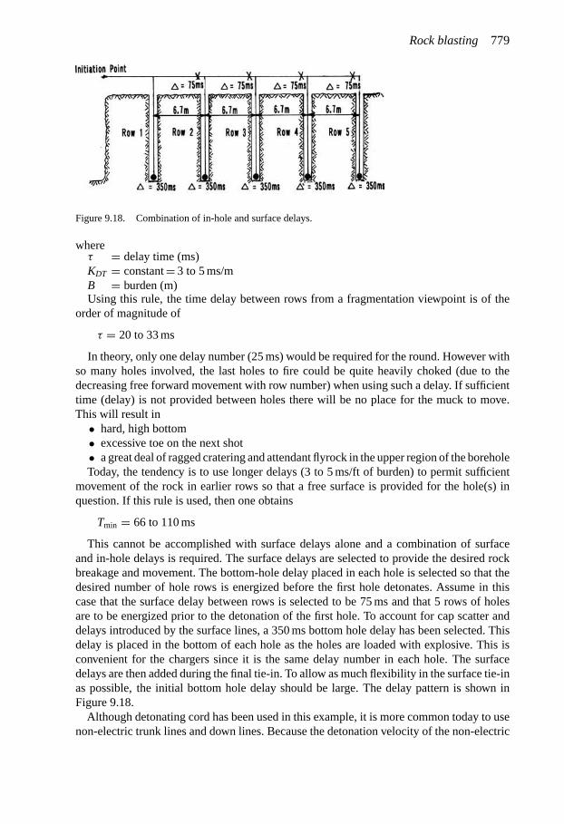
Rock blasting 779
Figure 9.18. Combination of in-hole and surface delays.
whereτ = delay time (ms)KDT = constant = 3 to 5 ms/mB = burden (m)Using this rule, the time delay between rows from a fragmentation viewpoint is of the
order of magnitude of
τ = 20 to 33 ms
In theory, only one delay number (25 ms) would be required for the round. However withso many holes involved, the last holes to fire could be quite heavily choked (due to thedecreasing free forward movement with row number) when using such a delay. If sufficienttime (delay) is not provided between holes there will be no place for the muck to move.This will result in
• hard, high bottom• excessive toe on the next shot• a great deal of ragged cratering and attendant flyrock in the upper region of the boreholeToday, the tendency is to use longer delays (3 to 5 ms/ft of burden) to permit sufficient
movement of the rock in earlier rows so that a free surface is provided for the hole(s) inquestion. If this rule is used, then one obtains
Tmin = 66 to 110 ms
This cannot be accomplished with surface delays alone and a combination of surfaceand in-hole delays is required. The surface delays are selected to provide the desired rockbreakage and movement. The bottom-hole delay placed in each hole is selected so that thedesired number of hole rows is energized before the first hole detonates. Assume in thiscase that the surface delay between rows is selected to be 75 ms and that 5 rows of holesare to be energized prior to the detonation of the first hole. To account for cap scatter anddelays introduced by the surface lines, a 350 ms bottom hole delay has been selected. Thisdelay is placed in the bottom of each hole as the holes are loaded with explosive. This isconvenient for the chargers since it is the same delay number in each hole. The surfacedelays are then added during the final tie-in. To allow as much flexibility in the surface tie-inas possible, the initial bottom hole delay should be large. The delay pattern is shown inFigure 9.18.
Although detonating cord has been used in this example, it is more common today to usenon-electric trunk lines and down lines. Because the detonation velocity of the non-electric

780 Open pit mine planning and design: Fundamentals
Figure 9.19. An idealized representation of the radialcracking surrounding a single hole.
lines is approximately half that of detonating cord, an additional time delay is introduced andshould be included in the calculations. The use of electronic delays eliminates the need toinclude detonating cap scatter in the calculations and offers considerable timing flexibility.
9.2.11 Determination of KB
Figure 9.19 shows the type of radial cracking which one might expect when blasting asingle hole in a brittle, massive rock formation. There will be relatively few long cracks(6–8) spaced uniformly around the hole. As one approaches the hole the cracks will beshorter and more numerous.
The maximum length (Re) of the radial cracks for a given explosive and rock type can beshown to be directly dependent on the hole radius. Thus as the hole diameter is increasedfrom 150 mm to 310 mm the length of the longest cracks would be expected to about double.This is consistent with the design relationship
B = KBD
presented earlier since the burden should be related to the lengths of the cracks generated
B ∝ Re (9.47)
If the strength of the explosive used in the hole of a given diameter is increased ordecreased, the outer crack radius should change accordingly. This is reflected in the valueof KB chosen.
As indicated, the key dimensions required in the development of a blast design are basedupon the burden which, in turn, is related to the borehole diameter through the burdenfactor KB.
B = KBD (9.26)
The value for KB
KB = 25
has been found by the present author and others (Ash, 1963), for example) to work well fora wide range of hole diameters when using ANFO in rocks of medium density (SG = 2.65).

Rock blasting 781
Figure 9.20. The rock volume associated with a blast hole.
Some guidance regarding the selection of KB when using explosives in rocks of other den-sities is needed. The approach described in this section is proposed as a first approximation.The development of the basic equation for KB will be first done using units of the metricsystem and then the equivalent formulae in the English system will simply be stated.
In addition to those parameters already introduced the following are needed.
SGE = specific gravity of the explosive
SGR = specific gravity of the rock
PFEXP = powder factor (kg/ton)
TF = tonnage factor (m3/ton)
The basic geometry is shown in Figure 9.20 where one blasthole from the round has beenisolated.
The number of tons (TR) broken is given by
TR = KSKHB2 × SGR × ρH2O (9.48)
where
B = burden (m)
ρH2O = density of water (mt/m3)
Since in the metric system
ρH2O = 1 mt/m3

782 Open pit mine planning and design: Fundamentals
this term will not be carried through the remaining equations. Knowing the powder factorrequired to provide the desired degree of fragmentation (PFEXP), the amount of explosiverequired (ERQD) is
ERQD = TR × PFEXP = KSKHB2 × SGR × PFEXP (9.49)
The total amount of explosive available (EAVL) is
EAVL = π
4(De)2[KHB + KJB − KT B] SGEXP (9.50)
where
De = explosive diameter (m)
Setting the amount of explosive required to that available yields
SGR KS KH B3 PFEXP = Bπ
4(De)2(KH + KJ − KT )SGEXP (9.51)
Solving equation (9.51) for B one finds that
B = De
[(π
4
)(SGE
SGR
)(1
PFEXP
)(KH + KJ − KT
KHKS
)]1/2
(9.52)
As can be seen by comparing equation (9.52) to equation (9.26), KB is equal to
KB =[(π
4
)(SGE
SGR
)(1
PFANFO
)(KH + KJ − −KT
KHKS
)]1/2
(9.53)
The powder factor based on the actual explosive used (PFEXP) will be replaced in equation(9.53) by the equivalent ANFO powder factor (PFANFO)
PFEXP = PFANFO
SANFO(9.54)
where
SANFO = relative weight strength of the explosive EXP to ANFO
Equation (9.53) then becomes
KB =[(π
4
)(SGE
SGR
)(SANFO
PFANFO
)(KH + KJ − KT
KHKS
)]1/2
(9.55)
This is quite a powerful formula. One of the major ways that the equation can be usedis to study the effect of changes in the explosive on the blasting pattern while keeping theother factors of the design constant. It can also be used to evaluate the effect of changingother variables. Rock density is one such parameter of interest.
9.2.12 Energy coverage
In examining the best type of “as-drilled” and “as-initiated” patterns to be used, consider-ation must be given to effective energy coverage of the volume to be fragmented and thenselection of the initiation geometry to make best use of the energy. The concept of cylindricalfragmented plugs of rock around each charge (in the absence of a free surface) is a usefultool in this regard. One considers the rock influenced by each blast hole to be bounded by
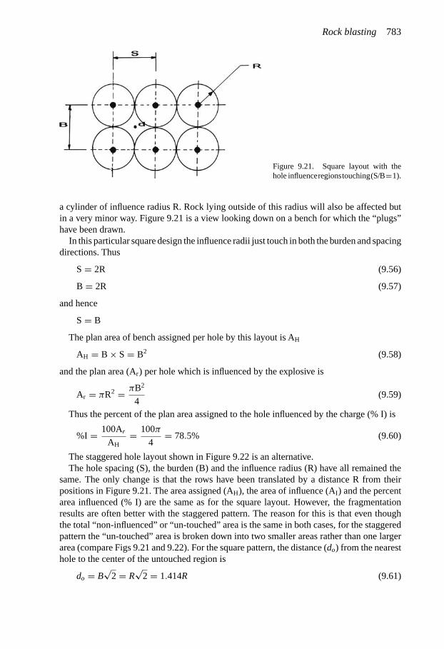
Rock blasting 783
Figure 9.21. Square layout with thehole influenceregionstouching(S/B=1).
a cylinder of influence radius R. Rock lying outside of this radius will also be affected butin a very minor way. Figure 9.21 is a view looking down on a bench for which the “plugs”have been drawn.
In this particular square design the influence radii just touch in both the burden and spacingdirections. Thus
S = 2R (9.56)
B = 2R (9.57)
and hence
S = B
The plan area of bench assigned per hole by this layout is AH
AH = B × S = B2 (9.58)
and the plan area (Ar) per hole which is influenced by the explosive is
Ar = πR2 = πB2
4(9.59)
Thus the percent of the plan area assigned to the hole influenced by the charge (% I) is
%I = 100Ar
AH= 100π
4= 78.5% (9.60)
The staggered hole layout shown in Figure 9.22 is an alternative.The hole spacing (S), the burden (B) and the influence radius (R) have all remained the
same. The only change is that the rows have been translated by a distance R from theirpositions in Figure 9.21. The area assigned (AH), the area of influence (AI) and the percentarea influenced (% I) are the same as for the square layout. However, the fragmentationresults are often better with the staggered pattern. The reason for this is that even thoughthe total “non-influenced” or “un-touched” area is the same in both cases, for the staggeredpattern the “un-touched” area is broken down into two smaller areas rather than one largerarea (compare Figs 9.21 and 9.22). For the square pattern, the distance (do) from the nearesthole to the center of the untouched region is
do = B√
2 = R√
2 = 1.414R (9.61)

784 Open pit mine planning and design: Fundamentals
Figure 9.22. Staggered layout withthe hole influence regions touching(S/B = 1).
Figure 9.23. Staggered layout withthe row influence regions touching(S/B′ = 1.15).
For the staggered pattern (Fig. 9.22), the figure abc constructed by connecting the nearestholes is an isoceles triangle. The sides ac and bc are of equal length. The point d whichis equi-distant from each corner lies along the altitude line. The distance from the threecorners is
d∗n = 1.2R (9.62)
In summary, even though the percent energy coverage has not changed with this staggereddesign, the un-touched area has been redistributed into two smaller pieces and the maximumdistance from any charge has been reduced from 1.414R to 1.2R. Thus the fragmentation isexpected to be better.
In reviewing the layout in Figure 9.22 it is obvious that the easiest way of reducing theuntouched area is to reduce the burden dimension while keeping the spacing constant. InFigure 9.23 the burden has been reduced until the radii of influence are just touching.
The center-to-center spacing to all adjacent charges is now equal to 2R. The triangle abcformed is an equilateral triangle with included angles of 60◦. The length (LA) of the altitudeof such a triangle is
LA = √3R (9.63)
which is just equal to the burden (B) dimension
B′ = √3R (9.64)

Rock blasting 785
Figure 9.24. The square pattern(S/B′ = 1.15) with contact in the rowdirection and overlap in the burdendirection.
Since the spacing is
S = 2R
the burden to spacing ratio is
B′
S=
√3R
2R= 0.866 (9.65)
The inverse of equation (9.65), the spacing to burden ratio, which is normally presented is
S
B′ = 2√3
= 1.155 (9.66)
The new bench area assigned to each hole with this layout is
AH ′ = 2R(√
3R) = 2√
3R2 (9.67)
The area influenced by the explosive is
Ar = πR2 (9.68)
and hence the percent coverage is
I% = Ar
AH ′= 100π
2√
3= 90.7% (9.69)
If the spacing
S = 2R
and burden
B′ = √3R (9.70)
are maintained but the rows translated with respect to one another to form a square layout,the result is as shown in Figure 9.24.
In the burden direction there is an overlap of the influence circles and in the spacingdirection, they just touch. The specific drilling (the number of drill holes per plan area) isthe same for both Figures 9.23 and 9.24. Now the area per hole affected by explosive energycan be shown to equal
AR =(
2π
3+
√3
2
)R2 (9.71)

786 Open pit mine planning and design: Fundamentals
Figure 9.25. Staggered pattern(S′/B′ = 1.0) with the spacingreduced to achieve total coverage.
while the assigned plan area to the hole is
AH = 2√
3R2 (9.72)
Thus the efficiency of the energy coverage is
I% = Ar
AH ′= 100
Ar
AH ′= 85.5% (9.73)
which is substantially less than for the staggered pattern. The distance from the nearestcharge to the center of the untouched region is, as before, also greater than with the staggeredpattern.
Beginning with the staggered pattern shown in Figure 9.23 one would now like to reducethe untouched area to zero. The condition that there should be no untouched region meansthat the distance dn from each corner to the midpoint should be the radius of influence R
dn = R (9.74)
Working through the geometry it can be shown that the new hole spacing (S′) should be
S′ = √3R (9.75)
This design is shown in Figure 9.25.There remains an untouched area because the burden has not as yet been adjusted.
Maintaining the ideal staggered geometry in which
B′′ =√
3
2S′ (9.76)
one finds that
B′′ = 3
2R (9.77)
Figure 9.26 is the result of reducing the burden from B′ to B′′ and the spacing fromS to S′.
As can be seen, the region untouched by the explosive charge has now vanished.
I% = 100%

Rock blasting 787
Figure 9.26. Staggered pattern(S′/B′′ = 1.15) with the burden reducedto achieve total coverage.
Table 9.1. Effect of drilling patterns and S/B ratios on the areacovered by the fracture circles. Equilateral triangular layout = 100%(AECI, 1978b).
S/B ratio Square pattern Staggered pattern% %
1 77 98.51.15� 76 1001.25 75 99.51.5 71 94.62.0 62 77
The layout area for each hole is now
AH ′′ = B′′ × S′ = 3
2
√3R2 = 2.6R2 (9.78)
as opposed to
AH = 4R2 (9.79)
in the original design shown in Figures 9.22 or 9.23. This means that the specific drillinghas increased by a factor of 1.54 while increasing the energy coverage from 78.5% to 100%.An alternative to this is to try and increase the radius of influence R by changing to a moreenergetic explosive.
Table 9.1 presents the relative efficiencies for different burden to spacing patterns. Theefficiencies given are relative to the pattern shown in Figure 9.27 which has an efficiencyof 100%. When examining patterns and pattern modification one must keep firmly in mind(a) the changes which occur in the specific drilling and (b) the practicality of drilling thepattern as designed.
As can be seen from Table 9.1, the staggered pattern produces a more uniform distributionof the fracture circles and thus more even fragmentation in the rock pile for the same powderfactor.
Optimum coverage is obtained with equilateral triangles, however it varies rather littleover the range from S/B = 1 to S/B = 1.5.

788 Open pit mine planning and design: Fundamentals
9.2.13 Concluding remarks
In this chapter, the authors have largely focused on ANFO since it is the most commonlyused blasting agent in mining operations today. There are a host of other explosives, par-ticularly pumped emulsions, which are finding favor. In this regard, the interested reader isencouraged to consult “The Blasters’ Handbook” (ISEE, 2011) and “Blasting Principles forOpen Pit Mining” (Hustrulid, 1999).
REFERENCES AND BIBLIOGRAPHY
Adel, G., Smith, B., Kojovic, T., Thornton, D., & J.M. Richardson. 2005. Mine-to-mill optimization ofaggregate production. Paper 05-009. SME Annual Meeting. Feb 28–Mar 2. SLC, UT.
Adel, G., Smith, B., Kojovic, T., Thornton, D., & J.M. Richardson. 2006. Application of mine-to-milloptimization to the aggregate industry. Paper 06-056. SME Annual Meeting. Mar 26–29. St. Louis, MO.
AECI, African Explosives and Chemicals Limited. 1978a. Parameters in surface blasting. Explosives Today.Series 2, No. 11, March.
AECI,African Explosives and Chemicals Limited. 1978b. Blasthole drilling and initiation patterns in surfaceblasting. Explosives Today. Series 2, No. 12, June.
AECI, African Explosives and Chemicals Limited. 1986. The design of surface blasts. Explosives Today.Series 2, No. 41, March.
Anonymous. 2011. Drill and blast – speaking the same language. Mining Magazine. April. pp. 34–36.Ash, R.L. 1963a. The mechanics of rock breakage (Part 1). Pit and Quarry. 56(2): 98–100.Ash, R.L. 1963b. The mechanics of rock breakage (Part 2) – Standards or blasting design. Pit and Quarry.
56(3): 119–122.Ash, R.L. 1963c. The mechanics of rock breakage (Part 3) – Characteristics of explosives. Pit and Quarry.
56(4): 126–131.Ash, R.L. 1963d. The mechanics of rock breakage (Part 4) – Material properties, powder factor, blasting
cost. Pit and Quarry. 56(5): 109–118.Ash, R.L. 1968. The design of blasting rounds. In Surface Mining (E.P. Pfleider, editor). AIME, New York.
pp. 373–397.Ash, R.L. 1992. Section 6.2.2 Design of Blast Rounds. In Surface Mining, 2nd Edition (B. Kennedy, editor).
SME, Port City Press, Baltimore. pp. 565–583.Atlas Copco. 2011. Blasthole Drilling for Open Pit Mining. 2nd Edition.Atlas Powder Company. 1987. Explosives and Rock Blasting. Maple Press. 662 pp.Badroddin, M., Khoshrou, H., and A. Siamaki. 2011. Prediction of burden at the Sungun Copper mine
by artificial neural network. Proceedings of the 35th APCOM. Wollongong NSW, Australia. September24–30. pp. 877–886.
Banda, R., & N. Rhodes. 2005. Electronic delay detonators-a unique solution to pertinent mining problems.JSAIMM. 105(9): 615–618.
Batten, C. 2009. Orica – Technology to Kick off a Career with a Bang. AusIMM New Leaders Conference.Brisbane, QLD. April 29–30. pp. 29–32.
Bedell, G. 2012. Personal communication. April.Bennett, J.W., Askraba, S., and P. Mackenzie. 2005. A New Method to Characterise Black Shales in Pilbara
Iron Mining Operations, Iron Ore 2005 Conference, Proceedings, AusIMM Publication Series 8/2005.Australasian Institute of Mining and Metallurgy, Carlton, Victoria, pp. 179–182.
Berry, L. 2011. Managing the drill and blast process. Paper 11-082. SME Annual Meeting. Feb 27–Mar 2.Denver, CO.
Bhushan, V., and P. Grouhel. 2007. Emerging Blasting Technology and Blast-Based Services, AUSIMMConference Proceedings, Large Open Pit Mining Conference Perth, WA, September 2007, pp. 19–24.
Bilodeau, M., Labrie, D., Bolsclair, M., Beaudoin, R., Roy, D., & G. Caron. 2007. Impact of electronicdetonators on downstream operations of a quarry. Paper 07-041. SME Annual Meeting. Feb 25–28.Denver, CO.
Boshoff, D., & R.C.W. Webber-Youngman. 2011. Testing stemming performance, possible or not?SAIMM. 111(12): 871–874.

Rock blasting 789
Cameron, A., Corkery, D., MacDonald, G., Forsyth, B., and T. Gong. 2007. An Investigation of AmmoniumNitrate Loss to Mine Discharge Water at Diavik Diamond Mines, AUSIMM Conference Proceedings,EXPLO Conference, Wollongong, NSW, September 2007, pp. 21–33.
Carter, R.A. 2008. Explosive situations. E/MJ. 209(6): 44–48. July/August.Caterpillar. 2012. Caterpillar Performance Handbook. Edition 42.Chadwick, J. 2005. Surface drilling and blasting: Big bangs. Mining Magazine. March. pp. 18–24.Clark, G.B. 1987. Principles of Rock Fragmentation. John Wiley and Sons, New York. 610 pp.Cook, M.A. 1958. The Science of High Explosives. Reinhold Publishing Corporation, New York. 440 pp.Cook, M.A. 1974. The Science of Industrial Explosives. Graphic Service and Supply, Inc. Salt Lake City,
Utah. 449 pp.E.I. DuPont de Nemours and Co. 1977. DuPont Blasters’Handbook. 175thAnniversary Edition. Wilmington,
Delaware. 494 pp.Ellenbecker, S. 2012. Smaller holes, patterns help control the blast. Mining Engineering. 64(5): 18–22.
May.Firth, I.R., & D.L. Taylor. 2001. Bench blast modeling using numerical simulation and mine planning
software. Paper 01-40. SME Annual Meeting. Feb 26–28. Denver, CO.Fjellsprengningsteknikk. 1974. Anders M. Heltzen, Chief Editor. Teknologisk Forlag, Oslo. 552 pp. In
Norwegian.Gustafsson, R. 1973. Swedish Blasting Technique. SPI Publishing. Gothenburg, Sweden. 327 pp.Harcus, M. 2011. Drill and blast: On the advance. Mining Magazine. April. pp. 16–33.Hudaverdi, T., Kulatilake, P., & C. Kuzu. 2011. A new model for blast fragmentation prediction based on
multivariate analysis. Paper 11-003. SME Annual Meeting. Feb 27–Mar 2. Denver, CO.Hustrulid, W. 1999. Blasting Principles for Open Pit Mining – Volume 1 General Design Concepts.
A.A. Balkema. Rotterdam. 382 pp.ISEE, 2011. Blaster’ Handbook 18th Edition. Society of Explosives Engineers. Cleveland, Ohio. 1030 pp.Jimeno, C.L., Jimeno, E.L., and F.J.A. Carcedo. 1995. Drilling and Blasting of Rocks. A.A. Balkema,
Rotterdam. 391 pp.Jimeno, C.L., Jimeno, E.L., and P.G. Bermúdez. 2003. Manual de Perforacion y Voladura de Rocas. U.D.
Proyectos. Madrid. 779 pp. In Spanish.Katsabanis, P.D., Gregersen, S., Kunzel, G., Pollanen, M., Pelley, C., & S. Kelebek. 2005. Effects of
blasting on damage and grindability of impacted rock. CIM Magazine. December 2005/January 2006.pp. 446–452.
Kim, K., & J. Kemeny. 2011. Site specific blasting model for mine-to-mill optimization. Paper 11-118.SME Annual Meeting. Feb 27–Mar 2. Denver, CO.
Komatsu. 2009. Specifications and Application Handbook. Edition 30.Langefors, U., and B. Kihlström. 1963. The Modern Technique of Rock Blasting. John Wiley and Sons.
New York. 405 pp.Little T.N. 2007. Flyrock Risk, AUSIMM Conference Proceedings, EXPLO Conference, Wollongong,
NSW, September 2007, pp. 35–43.Lovejoy, C. 2009. Management in action – Blasting technology: The big bang. Mining Magazine. May.
pp. 24–26.Lownds, C.M., & U. Steiner. 2010. Safety of blasting with electronic detonators. Paper 10-015. SMEAnnual
Meeting. Feb 28–Mar 3. Phoenix, AZ.Mandal, S.K., Singh, M.M., & S. Dasgupta. 2007. Air pressure and noise vis-á-vis detonating fuse. CIM
Magazine. May. pp. 95–100.Moore, P. 2006. Management in action – Surface blasting: Having a blast. Mining Magazine. November.
pp. 30–42.Moore, P. 2007. Equipment – Explosives: Explosives delivery. Mining Magazine. November. pp. 42–51.Moser, P., Lurf, R., and C. Weber. 2007. Operational Excellence in Rock Blasting – From a European Point
of View, AUSIMM Conference Proceedings, EXPLO Conference, Wollongong, NSW, September 2007,pp. 7–12.
Olofsson, S.O. 1997. Applied Explosives Technology for Construction and Mining. APPLEX,Ärla, Sweden.304 pp.
Onederra, I., Ruest, M., and G. Chitombo. 2007. Burden Movement Experiments Using the Hybrid StressBlasting Model (HSBM), AUSIMM Conference Proceedings, EXPLO Conference, Wollongong, NSW,September 2007, pp. 177–183.
UFM
|484
942|
1435
6130
16

790 Open pit mine planning and design: Fundamentals
Ozkahraman, H.T. 2010. Breakage mechanisms and an encouraging correlation between the Bondparameters and the friability value. JSAIMM. 110(3): 153–159.
Pereira, P.R. 2005. Better utilization of drilling and blasting resources to increase mining profitability. Paper05-114. SME Annual Meeting. Feb 28–Mar 2. SLC, UT.
Persson, P-A., Holmberg, R., and J. Lee. 1994. Rock Blasting and Explosives Engineering. CRC Press,Boca Raton, Florida. 640 pp
Potts, A. 2005. Equipment focus – Drilling and blasting: Boosting the bottom line. Mining Magazine.August. pp. 22–27.
Rantapaa, M., Mckinstry, R., & T. Bolles. 2005. Drill-to-mill: Efficient drilling and blasting resulting inincreased mill throughput at Barrick Goldstrike. CIM Magazine. January/February. pp. 160–162.
Refahi, A., Aghazadeh Mohandesi, J., & B. Rezai. 2009. Comparison between bond crushing energy andfracture energy of rocks in a jaw crusher using numerical simulation. JSAIMM. 109(12): 709–717.
Richards, A.B., and A.J. Moore. 2007. Effect of Blasting on Infrastructure, AUSIMM ConferenceProceedings, EXPLO Conference, Wollongong, NSW, September 2007, pp. 45–50.
Roy, D., Beaudoin, R., Bilodeau, M., Labrie, D., and G. Caron. 2007. Impact of Electronic Blasting Detona-tors on Rock Quarry Environment, Productivity and Energy Savings, AUSIMM Conference Proceedings,EXPLO Conference, Wollongong, NSW, September 2007, pp. 135–146.
Schwengler, B., Moncrieff, J., and P. Bellairs. Reduction of the Blast Exclusion Zone at the Black Star OpenCut Mine, AUSIMM Conference Proceedings, EXPLO Conference, Wollongong, NSW, September 2007,pp. 51–58.
Singh, R.K., Sawmiliana, C., & P. Pal Roy. 2007. Environmental impact of blast-emitted noise and airoverpressure: prediction and control measures. CIM Magazine. May. pp. 90–94.
Tamrock. 1989. Surface Drilling and Blasting. 477 pp.Thornton, D. 2009. The Implications of Blast-Induced Movement to Grade Control. Seventh Int, Mining
Geology Conf. Perth, WA. August 17–19. pp. 147–154.Thornton, D. 2011. Blast movement modelling and measurement. Proceedings of the 35th APCOM.
Wollongong NSW, Australia. September 24–30. pp. 397–309.Thornton, D. 2011. Blast movement monitoring – not just for grade control. AusIMM Journal. Issue 6. Dec.Wright, D. 2008. The Use of Electronic Detonators as a Key to Reducing Overall Mining Costs, AUSIMM
Conference Proceedings, The AusIMM New Leaders’ Conference Wollongong, NSW, July 2008,pp. 67–71.
Yang, R., and D.S. Scovira. 2007. A Model for Near-Field Blast Vibration Based on Signal Broadening andAmplitude Attenuation, AUSIMM Conference Proceedings, EXPLO Conference, Wollongong, NSW,September 2007, pp. 59–66.
Blasting References Especially Selected from the Proceedings, Annual Conferenceon Explosives and Blasting Technique, ISEE, Cleveland, Ohio. www.isee.org.
Arellano, M. & J. Delgado. 2001. Bench increase angle. Proceedings, 27thAnnual Conference on Explosivesand Blasting Technique, Jan. 28–31. Orlando, FL.
Arellano, M., E. Poulakidas & J. Flores. 2008. Efficient use of energy to wall control. Proceedings, 34thAnnual Conference on Explosives and Blasting Technique, Jan. 27–30. New Orleans, LS.
Christopherson, K. & V. de Viterbo. 2011. Trim blasting designs in the Morenci mine. Proceedings, 37thAnnual Conference on Explosives and Blasting Technique, Feb. 6–9. San Diego, CA.
Cunningham, C. 2002. Defining detonation energy for practical blasting. Proceedings, 28th AnnualConference on Explosives and Blasting Technique, Feb. 10–13. Las Vegas, NV.
Eloranta, J. 2001. Improved milling through better powder distribution. Proceedings, 27th AnnualConference on Explosives and Blasting Technique, Jan. 28–31. Orlando, FL.
Eloranta, J. 2002. The role of blast operations in metal mining. Proceedings, 28th Annual Conference onExplosives and Blasting Technique, Feb. 10–13. Las Vegas, NV.
Everett, W. & J. Eloranta. 2006. Digital delay blasting at United Taconite LLC. Proceedings, 32nd AnnualConference on Explosives and Blasting Technique, Jan. 29–Feb. 1. Dallas, TX.
Favreau, R. & P. Favreau. 2002. How to design a blast with computer simulations. Proceedings, 28th AnnualConference on Explosives and Blasting Technique, Feb. 10–13. Las Vegas, NV.

Rock blasting 791
Favreau, R. & P. Favreau. 2012. Evaluation of the fragmentation size distribution resulting from blastingas derived from basic principles. Proceedings, 38th Annual Conference on Explosives and BlastingTechnique, Feb 12–15. Nashville, TN.
Hendricks, C. 2002. The application of GPS positioning and drill monitoring technology. Proceedings, 28thAnnual Conference on Explosives and Blasting Technique, Feb. 10–13. Las Vegas, NV.
Hunter, M. 2003. Computerized drill for quarrying automates the drilling process. Proceedings, 29th AnnualConference on Explosives and Blasting Technique, Feb. 2–5. Nashville, TN.
Hustrulid, W. 2007. A practical, yet technically sound, design procedure for pre-split blasts. Proceedings,33rd Annual Conference on Explosives and Blasting Technique, Jan. 28–31. Nashville, TN.
Martin, P. 2004. Drill and blast optimization at the Sparkhule limestone quarry. Proceedings, 30th AnnualConference on Explosives and Blasting Technique, Feb. 1–4. New Orleans, LS.
Palangio, T. & J. Eloranta. 2007. Size matters in the Mesabi Range. Proceedings, 33rd Annual Conferenceon Explosives and Blasting Technique, Jan. 28–31. Nashville, TN.
Paley, N. & T. Kojovic. 2001. Adjusting blasting to increase SAG mill throughput at the Red Dog mine.Proceedings, 27th Annual Conference on Explosives and Blasting Technique, Jan. 28–31. Orlando, FL.
Paley, N. 2010. Testing electronic detonators to increase SAG mill throughput at the Red Dog mine.Proceedings, 36th Annual Conference on Explosives and Blasting Technique, Feb. 7–10. Orlando, FL.
Paley, N. 2012. Fragmentation from pattern expansion with electronic detonators at the Red Dog mine.Proceedings, 38th Annual Conference on Explosives and Blasting Technique, Feb. 12–15. Nashville, TN.
Paterson, L. 2000. Drilling efficiency and the associated benefits to the mining process. Proceedings, 26thAnnual Conference on Explosives and Blasting Technique, Feb. 13–16. Anaheim, CA.
Paventi, M., W. Lidken & L. Mirabelli. 2001. Mine automation program: Drill and blast analysis.Proceedings, 27th Annual Conference on Explosives and Blasting Technique, Jan. 28–31. Orlando, FL.
Preece, D. & S. Chung. 2002. Multi-blasthole, multi-row, detonation delay timing simulation of rock blastingusing DMCBLAST 3D. Proceedings, 28th Annual Conference on Explosives and Blasting Technique,Feb. 10–13. Las Vegas, NV.
Preece, D. 2008. 3D computer simulation of bench blasting with precise delay timing. Proceedings, 34thAnnual Conference on Explosives and Blasting Technique, Jan. 27–30. New Orleans, LS.
Proulx, R. & R. Pinksen. 2011. Oversize reduction project at the Iron Ore Company of Canada. Proceedings,37th Annual Conference on Explosives and Blasting Technique, Feb. 6–9. San Diego, CA.
Rogers, W., S. Kanchibotla, A. Tordoir, S. Ako, E. Engmann & B. Bisiaux. 2012. Understanding blastmovement and its impacts on grade control at Ahafo Gold Mine in Ghana. Proceedings, 38th AnnualConference on Explosives and Blasting Technique, Feb. 12–15. Nashville, TN.
Scott, D. 2012. An energy equality approach to blasting. Proceedings, 38thAnnual Conference on Explosivesand Blasting Technique, Feb. 12–15. Nashville, TN.
Spathis, A., G. Smith, I. Yacob & A. Labriola. 2001. Wall control at the Freeport Grasberg open cut mine:Vibration and gas penetration measurements as a precursor to improvements. Proceedings, 27th AnnualConference on Explosives and Blasting Technique, Jan. 28–31. Orlando, FL.
Vynne, J. 2001. Drill monitoring and GPS developments and their impacts on the drill to mill process.Proceedings, 27th Annual Conference on Explosives and Blasting Technique, Jan. 28–31. Orlando, FL.
Vynne, J, 2007. Drill monitoring & navigation systems at BHP’s Navajo mine. Proceedings, 33rd AnnualConference on Explosives and Blasting Technique, Jan. 28–31. Nashville, TN.
Vynne, J. 2011. Drill monitoring systems and the integration with drill & blast software. Proceedings, 37thAnnual Conference on Explosives and Blasting Technique, Feb. 6–9. San Diego, CA.
Wall, J. 2012. Perimeter control utilizing electronic detonators. Proceedings, 38th Annual Conference onExplosives and Blasting Technique, Feb. 12–15. Nashville, TN.
Webber, R. & S. Scovira. 2008. Record blast at Iron Ore Company of Canada. Proceedings, 34th AnnualConference on Explosives and Blasting Technique, Jan. 27–30. New Orleans, LS.
Wiggin, M. & L. Logan. 2001. Unlocking the wealth from benefit sharing in drill and blast. Proceedings,27th Annual Conference on Explosives and Blasting Technique, Jan. 28–31. Orlando, FL.
Williams, J. & K. Oakes. 2004. Blasting for wall control and stability using electronic detonators at BaldMountain mine, Nevada. Proceedings, 30th Annual Conference on Explosives and Blasting Technique,Feb. 1–4. New Orleans, LS.
Workman, L. 2001. Potential for the unifying of drilling, blasting and downstream operations by theapplication of technology. Proceedings, 27th Annual Conference on Explosives and Blasting Technique,Jan. 28–31. Orlando, FL.

792 Open pit mine planning and design: Fundamentals
Workman, L. 2003. The role of blasting in crushing and grinding efficiency and energy consumption.Proceedings, 29th Annual Conference on Explosives and Blasting Technique, Feb. 2–5. Nashville, TN.
Workman, L. 2007. Important considerations when selecting blasthole drills for high altitude use.Proceedings, 33rd Annual Conference on Explosives and Blasting Technique, Jan. 28–31. Nashville, TN.
Workman, L. & J. Eloranta. 2009. Considerations on the effect of blasting on downstream performance.Proceedings, 35th Annual Conference on Explosives and Blasting Technique, Feb. 8–11. Denver, CO.
Zink, C. 2006. Hole cleaning improvements through tricone bit lug design. Proceedings, 32nd AnnualConference on Explosives and Blasting Technique, Jan. 29–Feb. 1. Dallas, TX.
ACKNOWLEDGEMENTS
The authors would like to express their thanks to Geoffrey Bedell, Kennecott CopperCompany for reviewing the delay times used in the example. Thanks are also due to Ms.Arlene Chafe, Program Director, SEE Education Foundation, ISEE for making available tothe authors the Proceedings of the Annual Conference on Explosives and Blasting Tech-nique. The paper titles included under the REFERENCES are a very small sampling of theoverall selection for the period 2000 to 2012.
REVIEW QUESTIONS AND EXERCISES
1. Explain why it make sense to begin a discussion of the “Unit Operations” with blasting?2. What are the “design” components in blasting, drilling, loading and hauling?3. Discuss the relevance of the “mine to mill” concept.4. The blast design flowsheet logic has been presented. One begins with the “Design
Objectives”. Discuss the significance of each of the items listed. Is the list as presentedcomplete?
5. What is the difference between “deflagration” and “detonation”?6. The power released by the detonation of an ANFO charge 300 mm in diameter and 8 m
long has been determined. Repeat the calculation for a charge 381 mm in diameter and10 m long. Try to find the power output of a power plant in your vicinity. How does itspower output compare to this explosive charge? Conclusion?
7. You have been shown the derivation of a pressure-volume curve for ANFO. The energyreleased by the explosive is the area under the PV curve. Using the given PV curve, gothrough the steps to determine the energy. Does your result agree with that given?
8. If the confinement is low, much of the explosive energy is released to the atmosphererather than creating fractures in the rock. If the release occurs at a pressure of 4500 atm,how much energy has gone into fragmentation? How much goes into heave, air blast,etc.? What is your conclusion?
9. Define the terms:– Weight strength– Bulk strength– Relative weight strength– Relative bulk strength
10. There is some variance amongst different groups concerning the weight strengthassigned for ANFO. Check the literature from the major explosive suppliers and seewhat they give. What is the reason for the differences do you think?
11. In the literature there are differences in the values provided for ANFO density and alsothe velocity of detonation. Why is that? How does it affect you as a designer?

Rock blasting 793
12. The weight strength of an emulsion explosive A is given as 1.12 when compared toANFO which has a weight strength of 1.00. The specific gravity of explosive A is 1.17whereas forANFO the value is 0.80. What is the weight strength of explosive ‘A’relativeto ANFO?
13. Define the terms:– Burden– Spacing– Subdrill– Stemming
14. In Figure 9.6, the bench face is shown as vertical for simplicity. In a typical open pitmine, how might it really appear? How does this affect your design?
15. In some mines, the upper part of the hole, the “stemming” region, is left empty. In othermines it is filled with drill cuttings. In still others, special plugs are inserted. Discussthe differences one might expect in blast performance, if any.
16. Summarize the energy coverage approach to blast design.17. The proper placement of the detonator/primer in the hole is important. One common
rule is that it should be placed at the toe elevation. Why does this make sense?18. Summarize the Ash design rules. Learn/memorize the standard values for KB, KS, KJ,
KT and KH.19. How do you expect the fragmentation to depend on the hole diameter? If you wanted
to achieve a fine fragmentation in a massive rock, would large or small diameter holesbe better? Explain your reasoning using drawings?
20. In problem 19, would your answer change if the rock was jointed? Highly jointed?Explain.
21. In the Ash-based design formulas, the constant KB is used to relate the burden to thehole diameter. For ANFO in rock with density 2.65 g/cm3, KB = 25. What value wouldyou use for KB when explosive ‘A’ with a relative bulk strength of 1.15 is used? Hint:the suggested formula is
KB (explosive 2) = KB (explosive 1)
√ρ · s (explosive 2)
ρ · s (explosive 1)
22. At a particular open pit mine, the bench height is 35 ft, the hole diameter is 9′′ and therock has a specific gravity of 3.0. For ANFO and explosive ‘A’ determine:a. Burdenb. Spacingc. Subdrilld. Stemminge. Hole lengthf. Charge lengthg. Rock broken/hole (tons)h. Explosive factor (lbs/ton)
23. Discuss the difference between “as-drilled” burden and spacing and “as-shot” burdenand spacing. Is the explosive energy density affected? What differs?
24. If the following explosive prices apply, calculate the explosive cost/hole and per ton ofrock from the results of problem 22.– 1 lb cast primer = $4.50 each– Reinforced detonation cord = $150/1000 ft

794 Open pit mine planning and design: Fundamentals
– ANFO (bulk) = $50/100 lbs– Explosive A (bulk) = $70/100 lbs
25. At a surface mine in Canada, P&H rotary drills are used to drill 9′′ diameter holesto a depth of 39 ft. The bench height is 33 ft. The burden is 20 ft and the spacing is22 ft. ANFO (specific gravity of 0.85) is the primary explosive. The explosive factoris 0.50 lbs/ton or 1.08 lbs/bank cubic yard (bcy). Approximately 580 lbs of ANFO areused per hole.a. What is the specific gravity of the rock in place?b. Using the given data, what is the stemming length?c. How does this pattern compare with that suggested using the Ash-based design
guidelines?26. Blasting at a limestone mine is done using 6′′ diameter holes. Although the thick-
ness of the layer is 50 ft. thick, the benches are 45 ft high. There is a natural partingat the 45 ft. depth and no subdrilling is done to avoid dilution (the rock is used forcement production. The bench faces are vertical and back break accounts for 10% ofthe total tonnage. A single row of holes is used with S = 1.25 B. The explosive is ANFO(KB = 25), density = 0.85 g/cm3). The bank density of the limestone is 2.49 g/cm3,percent swell = 66%, swell factor = 0.60.a. What is the tonnage factor for the rock?b. What is the powder factor for this case?
27. If the bench height at a particular mine is 25 ft, what is the maximum recommended holediameter? The explosive is assumed to be ANFO (SG = 0.8). The rock has a density of2.4 g/cm3. Calculate the burden, spacing, subdrill and stemming. Draw a cross-sectionshowing the different dimensions. Calculate the explosive factor.
28. Define the following blasting terms:a. Powder factorb. Explosive factor
29. The in-place density of the rock at the Milly Dilly copper mine in British Columbiais 2.64 g/cm3. P&H rotary drills are used for drilling 10-5/8′′ diameter blast holes. Anemulsion explosive is used. It has a density of 1.2 g/cm3 and a weight strength withrespect to ANFO ρ = 0.85 g/cm3) of 0.87. In the hardest rock, a pattern 24 ft. × 27.6 ft(B × S) is used. The bench height is 40 ft, the subdrill is 5 ft and the stemming is 21 ft.A staggered pattern with S = 1.15 B is used.a. Why is a “staggered” rather than a “square” pattern used?b. Make plan and section drawings showing the blast pattern.c. Calculate the amount of rock attributed to each hole.d. Calculate the amount of explosive in each hole.e. Calculate the explosive factor (lbs/ton).f. What is the value of KB appropriate for this rock and explosive?g. How do the burden, spacing, stemming and subdrill values selected compare with
the Ash-based rules?h. The cost of the emulsion explosive is about $75/100 lbs. The cost of the recommended
12 oz primer is $4.00 and the Nonel downline (50 ft length) with detonator is $5.00.What would be the explosive cost per ton of ore?
30. A mine in the planning stages is trying to decide whether to use 12-1/4′′ or 15′′ diameterblastholes. The bench height has been fixed at 40′ and ANFO having of specific gravityof 0.85 will be used. Two rows of holes will be drilled. The rock has a specific gravity

Rock blasting 795
of 2.65. Design the blast patterns for each hole diameter (round off the distance to thenearest foot).a. Burdenb. Spacingc. Subdrilld. Stemminge. Hole lengthf. Loaded lengthg. Explosive/hole (lbs)h. Rock broken/hole (tons)i. Explosive factor (lbs/ton)j. Delay time (ms)
31. An explosive has a density of 1.1 g/cm3 and a weight strength relative to ANFO of 1.08.a. What would the value of KB be when used in rock of medium density?b. How should KB change when used in rock having a density of 3.1 g/cm3?
32. Discuss the effect of hole diameter and rock structure on fragmentation.33. Draw figures demonstrating the energy coverage of:
a. Square pattern, S/B = 1b. Square pattern, S/B = 1.15c. Square pattern, S/B = 1.25d. Staggered pattern, S/B = 1e. Staggered pattern, S/B = 1.15f. Staggered pattern, S/B = 1.25
34. The blasting agent ANFO (SG = 0.85) is being used as the primary explosive at a largemine. The bench height is 40 ft and the hole diameter is 9-7/8′′. A square pattern withB = S is being used. The rock has a bank density of 5200 lbs/yd3 and a loose densityof 3600 lbs/yd3. The powder factor is 0.68 lbs/ton. The subdrilling is 0.3 B and thestemming is 0.7 B.a. Draw a picture of the situation. Assume a vertical bench face. Label the drawing
carefully.b. Based upon the given powder factor calculate the burden being used.c. How does the value in (b) compare with that determined using the Ash-based
formula? What might be the reason for this?d. An emulsion explosive with a density of 69 lbs/ft3 and a weight strength of
SANFO = 0.9 has been suggested for testing. What would be the first pattern testedand why? What would be the expected result?
35. Much useful information concerning blasting and explosives is available on the Internet.In problem 33 an unidentified explosive with a density of 69 lbs/ft3 and a relative weightstrength of 0.9 has been suggested for testing. What commercial product might this be?Check the two websites: www.oricaminingservices.com and www.dynonobel.com.

CHAPTER 10
Rotary drilling
10.1 BRIEF HISTORY OF ROTARY DRILL BITS
Up until the beginning of the 20th century, the drilling of oil wells was done using bits ofvarious fishtail designs. One such design is shown in Figure 10.1.
As force is applied during bit rotation, the rock is literally scrapped away from the bottomof the hole. As one can imagine, this practice could and did work well in soft formationsbut in the harder, more abrasive formations the wear was high and the penetration rate low.In 1907, Walter Benona Sharp and Howard R. Hughes, Sr. were involved with drilling twotest oil wells at Goose Creek and Pierce Junction, Texas. According to the Handbook ofTexas (2012), both wells had to be abandoned because of the hard rock encountered. As aresult, the two men began to consider the possibility of developing a roller rock bit. It waseventually arranged for Hughes to proceed with the design and construction of a bit withcapital provided equally by Sharp and J.S. Cullinan. The result was the Sharp-Hughes rockbit (see Figs 10.2 through 10.4). In 1908, the Sharp-Hughes Tool Company was formed tomanufacture the bit and a factory was built at Houston, Texas. Hughes received 50 percentof the stock for his development of the bit and the other 50 percent was divided betweenSharp and Cullinan. In 1912, at the time of Sharp’s death, Hughes was given controllinginterest. Not long afterward, the company name was changed to the Hughes Tool Company.
As noted by Hughes in his patent application, the bit removes the rock by quite a differentprocess than the old fishtail bit. According to Hughes (1916).
“The edges, or cone points of the bit, roll in a true circle like a cone bearing, and crumbleor chip away the rock. The cone points, being of very hard steel, wear away slowly. Often
Figure 10.1. A typical fishtail bit design (Hughes, 1916).
796

Rotary drilling 797
Figure 10.2. Frontal view of the Sharp & Hughes rock bit.Hughes (1916).
Figure 10.3. Bottom view of the Sharp & Hughes cone bit. Hughes (1916).
they show but slight wear after drilling 50 ft. of rock, a few inches of which would completelydull the ordinary fishtail bit. The rolling motion allows the cutting edges on the cones tochip the rock, one edge after another.”
Figure 10.5 shows the Sharp & Hughes cone bit ready for operation.A number of major improvements have taken place over the years. In 1924, self-cleaning,
intermeshing cones were introduced which provided room for larger bearings and greatertooth depth (Fig. 10.6).

798 Open pit mine planning and design: Fundamentals
Figure 10.4. Drawings of the rock bit included in U.S. patent 930,759. Hughes (1909).
The introduction of ball and roller antifriction bearings lubricated only by the drillingfluid occurred in 1926. In 1929, bit life was increased by the application of tungsten carbidehard facing to cutter teeth. In 1934, a patent was issued for 3-cone bits (see Fig. 10.7. Asnoted in the patent application Scott and Garfield, 1934).
“It has heretofore been considered impossible and undesireable to form the teeth on thecutters of a three cone bit so that they may interfit in use, the reason being that it is difficultto make the rows of teeth in one cutter mate with the teeth of two other cutters, the teethof which must also interfit with each other. We have found that this may be done, andalthough the rows of teeth of each cutter are necessarily few, by proper arrangement theywill together cut the full bottom of the hole and provide a smooth running and fast cuttingdrill.”
Through this advance, the penetration rate and the bit footage essentially doubled.This patent, in practice, essentially “locked-up” the development of three-cone (tricone)
roller cone bits for the Hughes Tool Company until about 1951. In 1948, jet bits by whichhigh velocity streams of drilling fluid were directed against the hole bottom were introducedby the company. This facilitated cuttings removal and transport. In 1949, the use of air as

Rotary drilling 799
Figure 10.5. The Sharp & Hughes bit ready for operation. Hughes (1916).
the circulating medium for rotary blasthole drilling was introduced. With its introduction,many of the undesirable aspects of water such as
• availability• freezing• haulage• disposal
were eliminated. It was also found that air circulation resulted both in an increased pene-tration rate and bit life. The use of sintered tungsten carbide as the cutting elements wasintroduced in 1951. These inserts had the strength and crushing capacity to drill three toten times more hole than steel tooth bits in hard materials such as chert. Later, in 1959, thefirst practical sealed, pressure compensated, self-contained system of lubrication for rollerbearings was introduced. This was still an inadequate match to the life of the carbide toothbits. A new journal bearing the life of which matched that of the tungsten carbide cuttingstructures was introduced in 1969 by the Hughes Tool Company. Bit life was doubled,tripled, or even more. These time-line events were taken from Baker-Hughes (2007). As canbe seen, the development process has been one in which cutting element improvements havebeen followed by bearing improvements, followed by cutting element improvements, etc.

800 Open pit mine planning and design: Fundamentals
Figure 10.6. Self-cleaning cones as depictedin U.S. patent 1,480,014. Scott (1924).
The history of the use of rotary bits in mining spans a period of almost 70 years. Compactmachines designed specifically for rotary blasthole drilling were in use already in 1946.However, because of water circulation systems, their acceptance was very limited. Theintroduction of sintered tungsten carbide cutting elements in 1951 offered new possibilitiesfor economically cutting even harder rocks. Today rotary bits are used in the hardest forma-tion encountered in mining. Although mining users can still purchase steel tooth cutters, thecutting elements have largely been replaced by sintered tungsten carbide inserts of variousshapes and sizes. Figure 10.7 shows a few of the many possible insert designs. The interestedreader is also referred to Atlas Copco (2011e).
Figures 10.9–10.11 present pictures showing some modern tricone bits used for blastholedrilling. By comparing Figures 10.9 and 10.10 one can obtain a feeling of how bit design,in this case from the same manufacturer, has changed over a period of about 20 years.By comparing Figure 10.9a to 10.9b and Figure 10.10a to 10.10b one can clearly see themodifications in insert design and pattern needed to accommodate differing rock hardness.
Figure 10.11 clearly shows the required protection for the leg/shirttail of the bit.Figure 10.12 is a top view showing the intermeshing of the cones and inserts to get theproper bottom hole coverage. It is interesting to study this photo with respect to the com-ments regarding “impossibility” mentioned with respect to the patent of the tricone bit (seeFig. 10.7).
10.2 ROCK REMOVAL ACTION
Figure 10.13 is a diagrammatic view looking from the collar of the hole down on the cutterson the hole bottom. The three cones containing the cutting elements (either steel teeth or

Rotary drilling 801
Figure 10.7. The three-cone roller cone bit as depicted in U.S. patent 1,983,316. Scott et al. (1934).

802 Open pit mine planning and design: Fundamentals
Figure 10.8. Example of matching formation, insert shape, application and rock hardness. Security BitCatalog.
Figure 10.9a. Sandvik medium formation bit.Persson (1993).
tungsten carbide inserts) are made to roll along the hole bottom under the rotation of the drillstring. With the addition of an axial force (pulldown or weight) on the bit, the individualcutting elements in contact with the bottom begin to penetrate the surface.
Figure 10.14 is a diagrammatic representation of a section taken through one cone of atricone insert bit.
As the drill stem rotates, the cutting elements are successively forced into the surface.The idealized indentation on the bottom of the hole due to the penetration of cones A, B andC is shown in Figure 10.15.

Rotary drilling 803
Figure 10.9b. Sandvik hard formation bit. Persson (1993).
The actual pattern of indentations developed on the hole bottom by a rotary cone bitdrilling in Texas pink granite under laboratory conditions is shown in Figure 10.16. Theresemblance to the idealized breakage patterns is quite clear. Through good luck, a slabbroke off during the drilling offering a rare cross-sectional view of the bit at the bottom ofthe hole. The bit and inserts used in the test may be clearly observed in Figure 10.17.
To put these observations into the proper context, it is necessary to examine the rockremoval action for a single cutting element. Figure 10.18 shows an idealized view of asingle insert being pushed into the rock surface in a laboratory setting.
The first contact of the hemispherical indentor and the rock surface is at a single point.As one can easily imagine, since the contact area is very small, the stresses are very high. Inthe literature, the stresses developed when such surfaces first come into contact and deformslightly but elastically under the imposed loads are called Hertzian contact stresses. Theyare named after Heinrich Hertz whose original work “On the contact of elastic solids” waspublished in 1882 (Hertz, 1882). Since the rock is comparatively much weaker than theinsert and has a much lower elastic modulus, the interaction quickly changes from one ofelastic bodies in contact to one where rock failure occurs.
A thin crushed zone forms directly beneath the contacting point of the indenter. Thisis indicated as the “shell of recrystallized material” in Figure 10.18. This thin zone is intriaxial compression (very highly confined) and as a result very strong. It transmits a largelyradial pressure from the insert to the surrounding rock, which due to its lower (generallysmall) confinement, undergoes various degrees of compressive, shear and tensile failure.

804 Open pit mine planning and design: Fundamentals
Figure 10.10a. Soft formation bit. Sandvik Mining (2012d).
For example, it is very common to observe a tensile fracture extending downward into therock along the insert axis.
The zone of relatively high compressive stress and compressive failure is designated as“crushed zone of wedging material” in the figure. This zone grows in extent with increasingpenetration and in doing so it exerts a lateral and uplifting force on the adjacent rock.Radial cracks extend outward from the crushed zone. Eventually, the area of contact and thepressure are sufficient to wedge the adjacent material free and create chips. The chippingmay occur symmetrical to the insert point or asymmetrically. Chipping is the most efficientphase of the rock removal process and is to be encouraged.
The required depth of penetration for chipping to occur depends upon the cutting elementgeometry, the rock properties and the proximity of the adjacent craters. These chips oftenextend in depth to the ‘nose’ of the false wedge and hence the effective cutting depth can beconsiderably greater than the ‘penetrated’ depth. With the removal of the chips, the indentermoves down into the “false wedge” of crushed material below and the process continues. Ifthe depth of penetration is small, little or no chipping occurs and the drilling process is veryinefficient. Thus, there is a close relationship between the load on the bit, the insert design,and the proximity of adjacent craters which leads to an optimization of the rock removalprocess.

Rotary drilling 805
Figure 10.10b. Hard formation bit. Sandvik Mining (2012d).
Figure 10.19 shows a plan view of a rock surface in which several isolated indentationshave been made. It is clear that by careful spacing of the indentation locations that interactionwill occur and a large area of the surface will be affected.
When the hard metal insert bit first become a reality it was felt that the hemisphericalended or “round top” insert was best suited for drilling hard abrasive formations due to itsinherent strength. This shape along with complete bottom hole coverage has proven to betrue when drilling formations such as taconite. As the insert bit was used more universally,it became apparent that softer formations could be economically drilled with it. Round topinserts in conjunction with wider spacing were used to effectively do this job. In recentyears, the rock bit designer has found that “shaped” carbide inserts when properly utilizedwill give dramatic improvement in bit performance.
Inserts are made from a mixture of fine grained tungsten carbide powders which areblended with pure cobalt powder. The powders are pressed to shape and then liquid-phasesintered at about 2500◦F. At that temperature there is a liquor of cobalt and dissolved tung-sten carbide. When the part is cooled, a fully dense part is formed consisting of grains of

806 Open pit mine planning and design: Fundamentals
Figure 10.11. Medium – hard formation bit. Varel International (2012b).

Rotary drilling 807
Figure 10.12. Bottom view of a tricone bit showing the interlacing of the cutters. Atlas Copco Secoroc(2005).
Figure 10.13. View looking down on a three-cone bit.Chitwood (1970).
tungsten carbide cemented together by a binder of cobalt-tungsten-carbon. These materialsare referred to as “cemented carbides”. There are two basic characteristics of inserts madeof cemented carbides; hardness and fracture resistance. As the hardness is increased bydecreasing the cobalt content or decreasing the grain size, fracture resistance decreases.As the hardness is decreased by increasing the cobalt content or increasing the grain size,

808 Open pit mine planning and design: Fundamentals
Figure 10.14. Diagrammatic representation of one cone of a tricone bit showing the penetration of theinserts into the rock surface.
fracture resistance increases. Under applications involving high abrasion and low shockloading, inserts would require 90% tungsten carbide or higher. High shock loading appli-cations require grades with greater cobalt content. This is shown in Figure 10.20. Selectionof a proper grade for an application must be a compromise of wear and shock resistancequalities.
The cutting elements of the cone type bit are circumferential rows of teeth extendingfrom each cone and inter-fitting between rows of teeth on the adjacent cones. The sinteredtungsten carbide teeth are pressed into holes drilled in the cone surfaces. For the steel toothcutters, the teeth are machined from the basic cone material.
10.3 ROCK BIT COMPONENTS
A rolling cutter rock bits consist of four major components• the bit body• the cutters• the bearings• the bearing cooling/cuttings removal systemThe elements for a typical bit in Figures 10.21 and 10.22.

Rotary drilling 809
Figure 10.15. Idealized successive indentations on the hole bottom for a tricone bit with cones A, B and C.
Bit design has to start by recognizing that everything must fit into the hole being drilled.As a result it involves a series of trade-offs. In most instances one part can only be madelarger at the expense of making some other part or parts smaller.
As can be seen in Figures 10.21 and 10.22, the tricone bit is fabricated from three legs(lugs) each of which carries a bearing journal and cutter. The three legs and various com-ponents fit together to form the finished tool. Drilling a hole requires that the cutters workoutside the supporting parts. For this reason, rock bit journals are mounted at an angle. Thisangle is called the “journal angle” and is the angle formed by the center line of the journalintersecting a horizontal plane. The cutters are mounted on bearings which run on pins thatare an integral part of the bit body. Radial loads are absorbed primarily by the larger outerbearing element (either a roller bearing or a journal near the cone mouth) and the plainbearing in the cone nose. Ball bearings serve to retain the cones and in some instances toabsorb both radial and thrust loads. Additional outward thrust bearing capacity is providedby plain bearing surfaces at the inner end of the bearing pin and at the shoulder betweenthe ball race and nose bearing. The space allotted to the various components depends onthe type of formation to be drilled by the bit. Soft formation bits, for instance, which aregenerally run with less weight, have smaller bearings, thinner cone shells and thinner leg

810 Open pit mine planning and design: Fundamentals
Figure 10.16. Photo of the hole bottom showing the indentation/rock removal pattern. Tricone bit drillingTexas pink granite. Atlas Copco (2012a).
sections than hard formation bits. This allows more space for long toothed cutting elements.Hard formation bits which must be run under much higher weight on the bit to achieve therequired penetration, have stubbier cutting elements, larger bearings and sturdier bodies.Shirttail abrasion protection is standard on all blasthole bits. Without this wear resistantmaterial, bit shirttails would wear rapidly allowing the bearings to become exposed andshorten bit life.
10.4 ROLLER BIT NOMENCLATURE
The International Association of Drilling Contractors (IADC) first developed their codefor characterizing roller cone bits in 1972. The IADC code is updated periodically withthe most recent revision occurring in 1992. Every bit design is designated by a series ofthree numerals followed by an optional alphabetic letter (123A, for example). The basis forassigning each of these identifiers as described in information provided by Sandvik Mining(2012d) is summarized below:Character 1 reflects the type of cutter and the general formation hardness characteristic for
which the bit is considered best suited. One of eight numbers is assigned.• Numbers 1 to 3 apply to milled tooth bits• Numbers 4 to 8 apply to tungsten carbide insert (TCI) bits

Rotary drilling 811
Figure 10.17. Cross-section through the hole of Figure 10.16 showing the bit and the cutters. Atlas Copco(2012a).
Figure 10.18. Idealized indentor cratering model (Bauer and Calder (1967).
Within each series, the lowest number reflects the softest rock and the greatest number thehardest rock.Character 2 reflects the rock hardness sub-category. It ranges from 1 to 4 (softest to
hardest).

812 Open pit mine planning and design: Fundamentals
Figure 10.19. Plan view showing several isolated indentations made in a rock surface under laboratoryconditions. Atlas Copco (2012a).
Character 3 refers to the bearing design and the gage protection. The seven numberassignments are defined below:1. Standard, non-sealed roller bearing2. Roller bearing, air cooled3. Roller bearing, gage protected4. Sealed roller bearing5. Sealed roller bearing, gage protected6. Sealed friction bearing7. Sealed friction bearing, gage protected
Character 4 is optional and refers to optional available features:A. Air applicationB. Special bearing/sealC. Center jetD. Deviation controlE. Extended nozzlesG. Gage/body protectionH. Horizontal applicationJ. Jet deflectionL. Lug pads

Rotary drilling 813
Figure 10.20. Relative hard metal properties as a function of cobalt content. Chitwood (1970).
Air Water Separatoror Back Flow Valve
Pin Connection
Nozzle Nail Lock
Pin Shoulder
Shirttail Inserts
Lug
Gauge BevelInserts
Air Exit Slot
Cutter Cone
Gauge lnserts
Nose Inserts
Cone(L) andJournal (R)
Thrust Buttons
Inner RollerBearing
Ball Bearing
Outer RollerBearing
ShirttailHardfacing
Ball retainingPin Weld
Ball RetainingPin
Air Passageto Bearing
Nozzle
AirTube
Lock ring
Figure 10.21. Elements of a tricone bit. Atlas Copco (2011b,e).

814 Open pit mine planning and design: Fundamentals
PINCONNECTION
ANTIBACKFLOW
VALVE
SET SCAEW
JETNOZZLE
TUNGSTEN CARBIDEINSERT
CUTTER
ROLLER RACE
BALL HACE
THRUST FACE
FRICTION PIN RADIAL BEARING SURFACE
FRICTION PIN THRUST BEARING SURFACE
FRICTIONBUSHING
ROLLER BEARING RACE
BALL RACE
NOSETHRUST BUTTON BORE
FRICTION BUSHING BORENOTE: Specific bearing and air passage design can change from bit to bit dependent upon bit size
GAGE FACE INSERT
GAGE ROW INSERTGAGE FACE
THRUST BUTTON BEARING SURFACETHRUST BUTTON
SHIRTTAIL INSERTAIR PASSAGESROLLER BEARING
BALL BEARING
BALL RETAINING PLUG
BALL LOADING HOLE
BEARINGJOURNAL
SHIRTTAILHARDFACING
AIR PASSAGETO BEARINGS
LUG
AIR TUBE
TUNGSTEN-CARBIDEINSERT SHAPES
CHISEL (M-52 BIT) CHISEL (M-42 BIT)
CONICAL (M-73 BIT)HEMISPHERICAL
(M,74 AND M-85 BITS)
Figure 10.22. Blast hole bit components (Martin, 1982 and Reed Mining Tools, Inc.).
M. Motor applicationS. Standard milled toothT. Two-cone bit
W. Enhanced C/S
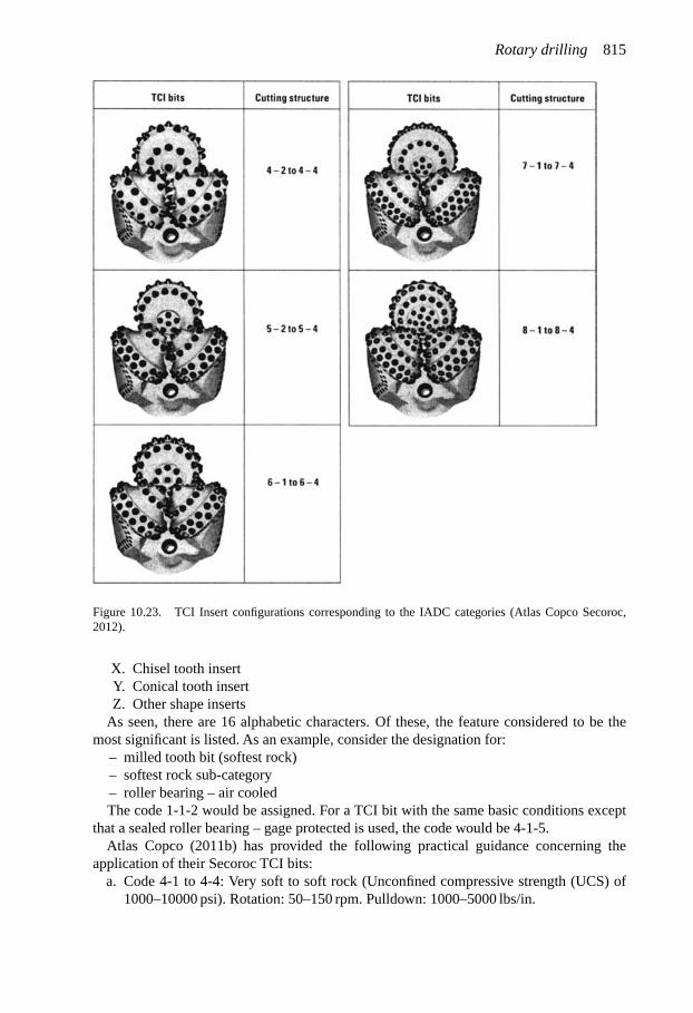
Rotary drilling 815
Figure 10.23. TCI Insert configurations corresponding to the IADC categories (Atlas Copco Secoroc,2012).
X. Chisel tooth insertY. Conical tooth insertZ. Other shape inserts
As seen, there are 16 alphabetic characters. Of these, the feature considered to be themost significant is listed. As an example, consider the designation for:
– milled tooth bit (softest rock)– softest rock sub-category– roller bearing – air cooledThe code 1-1-2 would be assigned. For a TCI bit with the same basic conditions except
that a sealed roller bearing – gage protected is used, the code would be 4-1-5.Atlas Copco (2011b) has provided the following practical guidance concerning the
application of their Secoroc TCI bits:a. Code 4-1 to 4-4: Very soft to soft rock (Unconfined compressive strength (UCS) of
1000–10000 psi). Rotation: 50–150 rpm. Pulldown: 1000–5000 lbs/in.

816 Open pit mine planning and design: Fundamentals
Figure 10.24. View of a large rotary blasthole drill (Pit Viper 351) with some key specifications. AtlasCopco (2011d).
b. Code 5-1 to 5-4: Soft to medium rock (Unconfined compressive strength (UCS) of6000–28000 psi). Rotation: 50–150 rpm. Pulldown: 3000–6500 lbs/in.
c. Code 6-1 to 6-4: Medium to medium hard rock (Unconfined compressive strength(UCS) of 22000–42000 psi). Rotation: 50–120 rpm. Pulldown: 4000–7000 lbs/in.
d. Code 7-1 to 7-4: Hard to very hard rock (Unconfined compressive strength (UCS) of36000–56000 psi). Rotation: 50–90 rpm. Pulldown: 4000–8000 lbs/in.
e. Code 8-1 to 8-4: Very hard to extremely hard rock (Unconfined compressive strength(UCS) of 48000–70000 psi). Rotation: 40–80 rpm. Pulldown: 6000–9000 lbs/in.
The bit designs corresponding to these codes are shown in Figure 10.23.
10.5 THE ROTARY BLASTHOLE DRILL MACHINE
A modern rotary blasthole drill is shown in Figure 10.24 together with some of thespecifications.
A diagrammatic representation of a crawler drill with key components identified isprovided in Figure 10.25.

Rotary drilling 817
Figure 10.25. Diagrammatic representation indicating key components. Martin (1982).
In Figure 10.25, the following components are denoted:A: MastB: Pipe rackC: Dust collection systemD: Top driveE: Drill pipeF: BitG: CabH: Machinery houseI: Leveling jacksJ: Crawlers
The functions that are performed by the machine are depicted in Figure 10.26.The functions and their activation/drive systems have been summarized by Martin (1982)
as follows:• Propel system, motors• Mast raising and lowering, hydraulic cylinders• Machine leveling, hydraulic cylinders• Bit rotation, motors• Bit pull down pressure, hydraulic cylinders or motors• Tool and pipe changing, hydraulic cylinders• Chip removal, compressed air• Dust control, optional systemsThe basic operations in the drilling process as outlined by Martin (1982) are:• The machine is propelled and maneuvered into position where the hole is to be drilled.
This has been previously determined by selection of a drilling pattern.• The mast is raised into position. For short distance moves, the mast is kept in the raised
position. As seen, the mast supports the drilling mechanism.• The machine is leveled into a horizontal orientation so that holes drilled are consistently
vertical (or at a specific angle). While drilling, the wheels (and/or crawlers) are raisedoff the ground.

818 Open pit mine planning and design: Fundamentals
Figure 10.26. Functions performed by the drilling machine.
• Drilling is performed by forcing the rotating drill bit into the ground with a high downpressure and rotary torque.
• With increasing depth, the drill pipe on which the cutting bit is fastened is extendedby adding additional lengths of drill pipe.
• Chips formed by the cutting action of the bit are removed from the hole by high velocityair fed down through the center of the drill pipe. The material chips are carried up thecircular space between the hole and the pipe.
• Blown out chips and fines are collected on the surface, around the top of the hole withthe air borne particles passed through a dust collection system.

Rotary drilling 819
• When the hole is completed to the desired depth, the bit is retracted with the drill pipeprogressively removed. The machine then starts the relocation sequence.
There are various ways of accomplishing these different activities. The main systemcomponents to be discussed are
• mounting• prime mover• rotation• pulldown and hoisting• circulation• mast and rod handling
Rotary blasthole rigs may be either crawler or truck mounted. Medium to large drillsare always crawler mounted. Rubber tired machines are primarily used when drilling ata number of sites separated by significant distances. Regardless of mounting, all drillrigs are leveled and supported by hydraulic jacks. These can be operated simultaneouslyor individually to correct for uneven ground conditions. Drill mobility and maneuver-ability is provided by the mounting. Mobility reflects the time spent going from holeto hole and is called the tramming speed. Maneuverability is the ability to position thedrill exactly where it should be. This often involves moving the drill in a very tight areaand positioning it over a pre-determined location. For re-drilling holes, the drill mustbe relocated exactly. The steering of crawler mounted drills is done by controlling thecrawlers. In some designs one crawler is locked while the other is engaged. In others,both crawlers can be operated, one in forward and the other in reverse. This gives a highdegree of steering control. Of increasing importance is drilling the hole at the positionand with the orientation desired, i.e. minimizing the hole deviation. Some sources of holedeviation are:
• accuracy of location• the type of ground (presence/orientation of rock structures, varying hardness, etc.)• the drill rig• the degree of instrumentation• the skill of the driller
The prime mover for the rotary rig is generally electric or diesel-hydraulic. Large crawlermachines use either AC or DC electric systems for the powered systems. Electric drills arecheaper to own, operate and maintain than diesel-hydraulic. The main advantage of thediesel machine is the elimination of the power cable. This allows flexibility to propel to anyarea without connecting or disconnecting electrical power.
A power cable reel and remote propel features are available which allows one person tooperate the drill (without the use of a helper). The power cable reels are electrical/hydraulicor air-operated. These are capable of reeling 2000 ft (600 m of trail cable). Power isrequired for
• tramming the rig from site to site• operating the jacks and erecting the mast• generating the pulldown force on the bit• rotating the bit• hoisting the bit• operating the air compressor(s)
In all cases, the machine leveling, mast raising/lowering and pipe handling systems employhydraulic cylinders. Many of the pulldown systems also use hydraulic cylinders.

820 Open pit mine planning and design: Fundamentals
The power required when drilling a hole of a particular diameter in a given material ismade up of two parts. The first part is the rotary power (PR) which is proportional to therotation rate (R) and the torque (T ).
PR = 2πRT (10.1)
where
PR = rotary power (in-lbs/min)R = rotation rate (revolutions/min)T = torque (in-lbs)
The second part, that associated with the feed (PF), is proportional to the pulldown force(PD) and the penetration rate (P).
PF = PDP = PdDP (10.2)
where
PF = feed power (in-lbs/min)PD = pulldown force (lbs)Pd = pulldown force/inch of bit diameterD = hole diameter (in.)P = penetration rate (in/min)
The total power applied is PT
PT = PR + PL = 2πRT + PdDP (10.3)
The required torque depends on the penetration of the inserts. For hard rock formations itwill be small whereas for softer rocks it will be high.
During drilling, the bulk of the power is consumed by the air compressor (for holecleaning) and the rotary drive. On most rigs, a single ‘prime mover’ drives the compressoroff of one end of its drive shaft and a “multi-pump” off of the other. The “multi-pump”drives will have two to four pumps, with two main pumps. One main pump will work theleft track and the rotation unit while the other main pump will work the right track and thepulldown system. Other pumps will run the compressor oil and engine coolant radiator fans(Atlas Copco, 2012a,b).
There are several methods for applying the required rotary torque to the drill string. Inoil well drilling this is done using a kelly bar system and a rotary table. For blasthole drills,the rotative power is applied by the top head drive directly to the end of the drill string. Thepower is applied by a gear drive or by a hydraulic or electric motor. The entire drive unit isattached to the drill string and moves up and down on tracks mounted on the mast. Whena new length of drill pipe is needed, the drive assembly is detached from the drill stringand raised to the top of the mast to permit inserting a new length of pipe. Normally rotaryspeeds will vary between 30 and 150 rpm. Many “soft” formation drilling operations go upto 150 rpm. Above that point, the bits begin to experience gage row carbide breakage (AtlasCopco, 2012a). Most drills are designed with a torque capability of between 10 and 20 ft-lbper 100 lb of down force.

Rotary drilling 821
Table 10.1. Minimum pulldown values used for preliminarydrill selection.
Bit Diameter, in. Pulldown, lb
5 20,0007 35,0009 60,00012 75,00015 120,000
All pull down systems use the weight of the drill rig to react against the down forceapplied to the bit. In general the drill rig will be capable of applying about 50 to 60 percentof its total weight. The total down force that can be applied to the bit depends not only onthe total rig weight but also how that weight is distributed. Balance of the drill is critical.Sufficient weight at the drill end to obtain rated down pressure without lifting the drill offthe jacks is mandatory. There are five different arrangements which are being employed toprovide the pulldown force in a top drive system.
• direct rack and pinion• direct chain and sprocket• chain and cylinder• rack and pinion with chain• cable and cylinderThe rack and pinion and the chain and sprocket systems are the most common. The chain
and sprocket system uses a hydraulically driven sprocket gear that engages and moves twocontinuous roller chains attached to both sides of the top-drive motor mounting. Anothersystem uses a driven pinion gear attached to the rotary drive unit that engages a rack mountedalong each side of the mast. This system eliminates the ‘softness’ of the chain or cableconnections between the head and the drive unit.
The rig should be capable of applying thrusts of 4000 to 9000 lb/in of bit diameter depend-ing on the size of the bit to be used. Table 10.1 presents some data for preliminary drillselection.
Air is supplied by one or more on-board compressors. Although in the past both• screw (medium pressure)• sliding rotary vane (low pressure)
were used, today only screw type compressors are employed. Single stage compressors cansupply air at 30 to 110 psi. P&H and Caterpillar/Bucyrus Erie drills are generally set toa maximum of 60 psi whereas Sandvik/Drilltech/Tamrock is set between 80–100 psi andAtlas Copco drills at 110 psi (Atlas Copco, 2012a,b). A two-stage unit can deliver bothlow pressure air at 30 to 60 psi and high-pressure air at 100 to 350 psi (some drills up to500 psi).
The heavier cuttings settle around the top of the hole, generally contained by flexiblecurtains. There are two basic types of dust control packages used on blasthole drills – waterinjection and dry-type. Water injection relies on a water tank to deliver 0.5 to 2 gpm of waterto the bit. Water injection generally will result in 15 to 20% shorter bit life depending onhow much water is used.
In a dry-type of unit, a fan is used to suck fine particles into a deck-mounted dust collectionsystem. Cyclones on filter bags may be used for fine particle separation.

822 Open pit mine planning and design: Fundamentals
Figure 10.27. Sandvik D90KS drill rig with the mast positioned for drilling angled holes in an Australianmine. Sandvik (2012d).
Masts are hinged and connected to hydraulic cylinders. This permits the mast to belowered, if necessary, when moving the drill rig. If the drill center of gravity is low, themove short, and the terrain suitable, the mast need not be lowered when moving.
Maximum hole depth is a function of mast height, which limits both the length of thedrill pipe and the amount of drill pipe that can be efficiently stored and handled.
In the past, drill pipe storage was provided, most commonly, by a vertical, rotatablecarousel holding fixture mounted on the front of the mast. Today, single pass drills have nocarousel. Rather some manufacturers provide one or two extra pipes in “pots” on the mast.
For most machines there is a choice of mast sizes available. These are generally givenin terms of the length of a drill stem (maximum hole depth in one pass) that they willaccommodate. The actual mast length is considerably longer than the stem length sinceit must include drill pipe, bit, stabilizer, rotary head, rotary coupling (swivel), bit basket,shock coupling, etc. The distance from the mast deck to the ground is approximately 5 feet.The bit, stabilizer and rotary coupling each add approximately another 5 feet. Hence a mastlength of about 75 ft is needed when drilling 50 ft in a single pass.
The front and rear of the drilling machine are specified with respect to the mast position.The front of the drill is that end which the operator would face when looking towards themast. Hence the rear of the machine is that closest to the hole.
If the drilling pattern requires angled holes, the mast can be tilted from the vertical. Theangles can vary from 0 to 15 or 30 degrees generally in 5 degree increments. The mast ispinned into position during actual drilling. Figure 10.27 shows one drill rig with the mastset for the drilling of angled holes.
Angle hole drilling can be advantageous under some circumstances. Angle drilling isreported to
• minimize back-break• increase breakage at the toe• yield better fragmentation• reduce noise and shock waves

Rotary drilling 823
However• production may decrease since pull down capacity is reduced.• the drill pipe will impede cuttings outflow as the pipe rubs on the bottom side of
the hole.• pipe connections are also slower.• maintenance costs may increase with angle hole drilling as well.• the bit and drill string striking against the bottom side wall of hole may induce vibration
to the machine.• other factors to consider are the higher capital expense for angle hole attachments and
auxiliary equipment.An old rule of thumb is that angle hole drilling reduces production output by about 20%
and possibly, because of this, angle drilling is still seldom used in metal mining. Angledrilling is, however, often used in the cast blasting of coal overburden with very goodresults.
10.6 THE DRILL SELECTION PROCESS
Drill selection is a three step process. The first step involves the identification, in general,as to the type and size of drill required. A number of factors enter into deciding what sizeof drill to purchase (Nelmark (1983):
• Type of material. A good estimate of drillability is essential from the beginning of amine study. As many core drilling samples as economically possible should be taken.Rock sample tests in laboratory conditions have correlated quite well with the actualdrillability of material. With this type of information and material hardness, the numberand size of drill units can be predicted.
• Production requirements. Knowing the volume of material to be moved along withtype of material determines size and number of drills as well.
• Size of loading equipment, haulage and plant. This information determines the requiredratio of drills to that particular equipment. Pit geometry, haulage restrictions, crushingcapacity and fragmentation all enter into the decision making process.
• Bank height. This usually is determined by loading equipment, but the mine planshould take into account the single-pass capabilities of the drill or the depth of drillingif multiple passes are used on blast hole drill specifications.
• Blasting requirements. Drill hole patterns based on hole size, formation, burden,spacing and hole depth all factor into model selection.
• Environmental restrictions. Blast vibration levels and noise restrictions may be impor-tant in determining the size of hole to be drilled. Often these restrictions become allencompassing.
• Overall cost. When selecting the drill, all elements of cost must be analyzed and notjust the initial capital equipment expenditure. This applies to maintenance, power;blasting, re-usables such as bits, drill pipe and drill collars, lubrication, labor; anddepreciation. All of these factors will enter into selecting a drill for lowest overall cost.
The number of drills to be purchased is also a decision which needs to be made. Typicallyone drill is needed for each shovel. However, where pit layout requires great propel distancesbetween drill patterns, an extra drill may be necessary.
In step two, the potential suppliers of the appropriate drill are identified.

824 Open pit mine planning and design: Fundamentals
In step three, the factors entering into the selection process become much more specific.Some of the considerations which might be added are (Martin, 1982):
• Machine capabilities (pulldown, rotary torque, etc.) must exceed formation penetrationrequirements.
• Maximum hole size capability increases with machine size.• Larger machines are more rugged and can generally drill in harder formations.• A machine that can handle drill pipe long enough to permit single pass drilling can
significantly improve productivity.• The production rate is dependent both on the actual penetration rate and on the time
required for pipe changes and machine repositioning.• Electric drives have the lowest operating cost, the longest service life and the best track
record for reliability.• Electric drives require an in-pit power distribution system.• Three levels of pit and area mobility are available; low speed crawlers (electric
machines), medium speed crawlers (diesel machines) and roadable high speed carriers(wheel mounted units).
• Dust control requirements are dictated by regulations.• Optional equipment such as powered cable reels, automatic lubrication, automated
controls, etc., can increase the efficiency of the drilling operations.• Long term productivity is dependent on the ruggedness, reliability and maintainability
of the design.Special consideration must also be given to mine life, ruggedness of the terrain, the
frequency and distance of moves between drilling locations, the availability of skilled oper-ating and maintenance personnel, and maintenance and service support facilities. These areall examined and compared with the information contained in specification sheets (Martin,1982).
Figures 10.28 through 10.30 present the specification sheets associated with a largerotary drill.
10.7 THE DRILL STRING
The pulldown force as well as the rotational torque are transmitted from the drill rig on thesurface through the drill stem to the bit. The parts which make up the drill string are shownin Figure 10.31.
Drill stems vary in length from 15 to 55 ft. The current trend is to provide a mast/derrickhigh enough to permit use of only one drill rod for the depth of the hole selected. Somerigs, however, provide a semi-automatic feed rack, which simplifies adding and removingsections of drill stem. Drill stem connections are called “tool joints” and are usually of theBECO thread type for drill pipe 5′′ and larger in diameter.
The blast hole drill stem is normally a flush OD member with a threaded connectionat each end (male end = pin, female end = box). It has wrench slots at one or both endsfor “make-up” or “break-out” with another threaded connection. Table 10.2 provides thedimensions for standard drill pipe.
Drill stems are usually chosen of sufficient size to give an adequate annulus velocityfor cuttings removal. That size is generally sufficient to provide the necessary torquecapacity. On air circulation rigs, the diameter of the drill stem should, at a minimum,

Rotary drilling 825
Figure 10.28. Specification sheet (1) for a P&H 250 XPC electric rotary blasthole drill. P&H (2012a).
be 1-1/2 to two inches smaller than the hole diameter to (1) allow for cuttings transport,and (2) reduce the chance for sticking in the hole. Stems 2 to 3 inches smaller in diameterthan the bit diameter are to be preferred since this provides a nice open annulus facilitatingcuttings removal. Table 10.3 provides some typical bit diameter – pipe outer diameter (O.D.)combinations.
A bent stem will cause excessive vibration, undue stress in the drive train and usuallycauses uneven wear on rock bit cutters. For long steel life and overall economy, the thickestwall should be selected which is consistent with the limitations of the drill or the operation.

826 Open pit mine planning and design: Fundamentals
Figure 10.29. Specification sheet (2) for a P&H 250 XPC electric rotary blasthole drill. P&H (2012a).
The resistance to buckling of steel used in compression is a function of the wall thicknessand diameter of the tube. Table 10.4 provides some common dimensions for drill pipe.
Whenever practical, the drill string should be made up of two identical lengths of drillsteel with a 36′′–48′′ long “stabilizer sub” (see Fig. 10.31) located between the lower drill

Rotary drilling 827
Figure 10.30. Specification sheet (3) for a P&H 250 XPC electric rotary blasthole drill. P&H (2012a).
stem and the bit. The “sub” takes 95% of the erosion and is much cheaper to replace thanthe lower pipe. Once the lower pipe is worn, it can be swapped with the upper pipe. It isnormal to replace 5–10 bit saver subs before you need to switch pipe pieces (Atlas Copco,2012a).

828 Open pit mine planning and design: Fundamentals
SmoothdriveTM
shock absorbingsub
Welded strapmethod
Square driveflange method
EZ-DrillTM
roller stabilizerDuralloyTM
bit sub adaptor
CenterollTM
rotary deck bushing(repairable)
Secoroc Tricone bits
Full length repairableTeamalloyTMbody drill pipe
(box-box optional)
Threadsaversub
SmoothdrillTM
shock absorbingsub
Figure 10.31. Components of a typical drill stem and drill stem stabilization system. Atlas Copco (2011c).
The following should be considered in the selection of drill steel (Nelmark, 1983), Toll(1981):
1. Drill hoisting capacity2. Size and depth of hole to be drilled3. Volume of circulation media available4. Torsion, compression or tension loading5. Makeup and breakout wrenching availableWhen drilling blastholes with a top drive rotary head configuration, the drill string tends
to behave as a slender column and can be quite susceptible to buckling. The bit effectivelyacts as a bottom pivot point for the column. Any column buckling and hence rotationabout this pivot point causes angular misalignment of the bottom hole assembly and gives

Rotary drilling 829
Table 10.2. Standard blasthole drill pipe sizes for use in surface mining applications. (Sandvik, 2012c).
Outer Outer Nominal Nominal Nominal Nominaldiameter diameter wall wall weight weightO.D. (ins) O.D. (mm) Thickness (ins) Thickness (mm) (lbs/ft) (kg/m)
3 76.2 0.2 5.16 6 90.28 7.01 8 12
3 1/2 88.9 0.22 5.49 7 100.3 7.62 10 15
4 101.6 0.28 7.15 11 161/2 12.7 19 28
4 1/2 114.30 0.29 7.33 13 190.34 8.56 15 221/2 12.7 21 313/4 19.05 30 451 25.4 37 55
5 127 1/2 12.7 24 369/16 14.29 26 393/4 19.05 34 511 25.4 43 64
5 1/2 139.7 1/2 12.7 27 403/4 19.05 38 57
6 152.4 3/4 19.05 42 631 25.4 53 79
6 1/4 158.8 1/2 12.7 31 463/4 19.05 44 65
6 1/2 165.1 3/4 19.05 46 681 25.4 59 88
7 177.8 3/4 19.05 50 741 25.4 64 95
7 5/8 193.7 7/8 22.23 63 941 25.4 71 106
8 5/8 219.1 1 25.4 82 1221 1/2 38.1 114 170
9 1/4 235 1 25.4 88 1311 1/2 38.1 124 185
10 3/4 273.1 1 25.4 104 1551 1/4 31.75 127 1891 1/2 38.1 148 220
12 3/4 323.9 1 25.4 127 18913 3/8 339.7 1 1/4 31.75 163 243
1 1/2 38.1 192 286
off-center load concentrations on the bit. This off-center distribution of down thrust on thebit causes three undesirable effects (Toll, 1981).
1. The full thrust is shifted from one cone to another as the bit rotates. This overloads thecone teeth or carbide buttons which rapidly shatter and break up.
2. The overload down thrust on the cone is transferred to cyclic thrust along the axis of thecone bearing pin as the bit rotates. This thrust can increase to the point where the balland nose bearings are over stressed and the ball flange breaks down with the overallresult of premature bearing failure.

830 Open pit mine planning and design: Fundamentals
Table 10.3. Various combinations of hole diameter and pipe diameter (Atlas Copco 2011f).
Hole diameter (ins) Pipe O.D. (ins) Hole diameter (ins) Pipe O.D. (ins)
5 5/8 2 7/8 9 7/8 73 1/2 7 3/44 8 5/8
5 7/8 2 7/8 93 1/2 10 5/8 74 7 3/4
6 2 7/8 8 5/83 1/2 94 11 7
6 1/4 3 1/2 7 3/44 1/2 8 5/85 9
6 3/4 3 1/2 12 1/4 74 7 3/44 1/2 8 5/85 9
7 3/8 3 1/2 13 5/8 104 1/2 10 3/45 1/2 15 10
7 7/8 3 1/2 10 3/44 1/2 125 1/2 136 1/2 16 106 5/8 10 3/47 12
9 4 1/2 135 1/2 17 1/2 106 5/8 147 167 3/4
3. The outside gauge cutting teeth or carbide inserts are the most heavily overloaded of allcone teeth. These break up and the cone assumes an “apple shape”. Bit life is severelyreduced and bits worn in this manner tend to drill undersize holes.
The same overall effect is evident when the bit exhibits a tendency to follow structuralplanes and transfers a bending moment to the drill string. This, once again, results in angularmisalignment. The common expression for this type of behavior is “coffee-grinding” (Toll,1981). To prevent the bit acting as the rotation point, a stabilizer is used just above thebit (see Fig. 10.31). Theoretically the guiding elements should have the same diameter asthe bit. Unfortunately this is not practical because of the normal attrition of rock bit gagewear surfaces. The stabilizer should therefore be held at the largest diameter practicable.Concentricity of the guiding elements is important. Eccentricity in these guiding elements isas detrimental to drill performance, rock bit life, and drill pipe life as adequate stabilizationis beneficial. There are two types of stabilizers
• bar or fixed blade stabilizers• roller stabilizers

Rotary drilling 831
Table 10.4. Common drill pipe dimensions. Sandvik (2012c).
Outer diameter Nominal wall Nominal wall Nominal weight Nominal weightO.D. (ins) O.D. (mm) Thickness (ins) Thickness (mm) (lbs/ft) (kg/m)
3 76.2 0.2 5.16 6 90.28 7.01 8 12
3 1/2 88.9 0.22 5.49 7 100.3 7.62 10 15
4 101.6 0.28 7.15 11 161/2 12.7 19 28
4 1/2 114.30 0.29 7.33 13 190.34 8.56 15 221/2 12.7 21 313/4 19.05 30 451 25.4 37 55
5 127 1/2 12.7 24 369/16 14.29 26 393/4 19.05 34 511 25.4 43 64
5 1/2 139.7 1/2 12.7 27 403/4 19.05 38 57
6 152.4 3/4 19.05 42 631 25.4 53 79
6 1/4 158.8 1/2 12.7 31 463/4 19.05 44 65
6 1/2 165.1 3/4 19.05 46 681 25.4 59 88
7 177.8 3/4 19.05 50 741 25.4 64 95
7 5/8 193.7 7/8 22.23 63 941 25.4 71 106
8 5/8 219.1 1 25.4 82 1221 1/2 38.1 114 170
9 1/4 235 1 25.4 88 1311 1/2 38.1 124 185
10 3/4 273.1 1 25.4 104 1551 1/4 31.75 127 1891 1/2 38.1 148 220
12 3/4 323.9 1 25.4 127 18913 3/8 339.7 1 1/4 31.75 163 243
1 1/2 38.1 192 286
The bar (or fixed blade) type of stabilizer consists of a sub the same diameter as thedrill stem and approximately three to four feet long. Three to four blades are welded to thestabilizer body so that they will be the same diameter as the hole being drilled. Pelletizedtungsten carbide can be applied to the blades to resist abrasion. The wear rate can beexcessively high in hard, abrasive formations due to the scraping action against the holewall. This necessitates frequent rebuilding. Blade stabilizers should be changed every time anew bit is put on the string. In practice blade stabilizers are usually changed every second orthird bit to reduce lost time due to changes and to defray the purchase price of the stabilizer.Blade stabilizers can be rebuilt or the rings can be replaced.

832 Open pit mine planning and design: Fundamentals
In roller stabilizers, the rollers are mounted on and freely rotate about large diameter toolsteel bearing pins which are cooled by the circulating air. The guiding elements in this toolroll against the bore wall, providing close-to-hole wall stabilization while minimizing bothattrition and torque requirements. Normally the rollers contain tungsten carbide inserts toresist wear. This assembly maintains gauge and effective stabilization for 15,000 to 20,000 mof drilling depending on tool size and ground conditions.
Stabilizers help to maintain a straight hole and produce a beneficially smooth bore. Byacting as a guide, a properly sized stabilizer forces the drill bit to rotate about its own center,thereby utilizing the energy directed to it in the most efficient manner. Figure 10.31 showsa stabilizer assembly. As indicated, the blades or rollers acting on the hole walls effectivelyact as constraints on movement in the horizontal plane. The bottom hole assembly and stemcolumn is stiffened by this constraint. The top of the stabilizer becomes the pivot point ratherthan the bit. The advantages are:
• if buckling were to occur it would not misalign the bit• rod buckling would require a higher load because of the extra stiffness• the blades or rollers act on the hole wall to resist any bending moment which might
result from the bit tending to follow structural planes• it allows higher down thrusts to be applied to the bit which means higher penetration
rates while bit life remains relatively constant.The major point of drill stem constraint apart from in-hole stabilizers and the point of
attachment to the rotary drive head is the point at which the drill stem passes through theworking deck of the drill rig (see Fig. 10.31). Constraint provided by deck bushing must befirm and concentric while allowing free stem rotation. Earlier, the most successful bushesfor this point were made of hard cast iron (Toll, 1981). Manufacturers are now producingroller bearing equipped rotary deck bushes.
A vibration dampener is a resilient coupling used between the drill and the drill pipe ontop drive machines to dampen shock loads created by the bit action (see Fig. 10.31). It ismost beneficial when drilling in fractured formations, intermittent hard and soft layers, orhard formations (Toll, 1981). The following benefits occur
• reduction in drilling machine maintenance by dampening torsional and axial shockloads.
• increases drilling rates by keeping bit in more uniform contact with the formationallows the use of more weight and higher rotary speeds in rough drilling areas.
• increases bit life by dampening cyclical shock loading normally transmitted to the bitbearings and cutting structure
• decreases operator noise by eliminating the metal to metal contact between rotary driveand the drill pipe.
10.8 PENETRATION RATE – EARLY FUNDAMENTAL STUDIES (Morris 1969)
In 1969, Morris (1969) reported the results of a series of studies aimed at the developmentof a drillability index for ‘hard’ rock mining roller cone rotary bits. A 90 degree conicaltungsten carbide compact with a 1/8 inch radius at the apex (Fig. 10.32) was mounted in asimple hydraulic press (Fig. 10.33).
This tungsten carbide compact was chosen as a test element to duplicate the drill bitelement of a hard rock mining bit. The compact was pressed into a smooth, flat surface of a

Rotary drilling 833
Figure 10.32. Bit element used in the laboratory experiments conducted by Morris (1969).
Figure 10.33. Hydraulic pump and ram with single carbide bit element. Morris (1969).
number of control samples with the hydraulic ram. The penetration (P) was recorded at loadincrements of 500 lbs up to a maximum load of 5000 to 6000 lbs which was considered torepresent the maximum load per insert experienced in actual drilling situations.
A typical force-penetration curve is plotted in Figure 10.34.As can be seen, the penetrationis a direct function of load up to the threshold force, E. There, due to extrusion of the crushedmaterial from under the bit element, the penetration increases sharply.
The slope of the force-penetration curve to point E may be taken as a measure of rockstrength under a hemispherical bit element. However, the relationship between actual craterdepth (P′) and the threshold force (E) was thought to be more directly related to the drillabilityof the roller-cone bit. As indicated by Morris (1969), roller-cone bits drill most efficientlyat a bit load in excess of a certain minimum threshold force (That load is considered to berelated to the single bit element threshold force of the static penetrator test). In practice,Morris (1969) found that adequate penetration rates can be maintained at weights below

834 Open pit mine planning and design: Fundamentals
Figure 10.34. Typical penetration versus applied load curve for the 1/8 in. sphere. Morris (1969).
the static threshold weight. Dynamic loading, a relatively rough hole bottom, and the factthat all bit elements are not equally loaded lowers the effective threshold weight in actualdrilling. For these reasons, the ratio P′/E, rather than the slope of the force-penetration curve(P/E) as the drillability index.
Drillability index = P′/E (10.4)
Experience (Morris (1969)) has indicated that ground with a drillability index greaterthan 0.00002 in/lb can be successfully drilled with steel tooth roller bits or cutters whereasdrillability index values less than 0.00002 in/lb dictate the use of tungsten carbide insertbits. By multiplying the static threshold force (E) by the average number of bit elementsworking (I), one arrives at an effective drilling weight.
W = EI (10.5)
where
E = static threshold forceI = average number of bit elements in contact
The number of bit elements in contact with the rock surface at any one time dependsupon the
• bit-type (design)• size• average bit penetration per revolutionObservations such as shown in Figure 10.35 reveal that
I = 0.08C (10.6)
where
C = total number of bit elements

Rotary drilling 835
Figure 10.35. The inserts in contact with the bot-tom of the hole (Bauer and Calder (1967)).
Table 10.5. Number of bit elements working at any time (After Morris (1969)).
Insert bits Tooth bits
Size Type I Type I
6-3/4′′ H8M 10 H7M 14H10M 14
7-7/8′′ H8M 10 H7M 14H10M 17
9′′ H8M 12 H7M 18H10M 18
9-7/8′′ H8M 16 H7M 22H10M 19
10-5/8′′ H8M 17 H7M 22H10M 21
12-1/4′′ H8M 18 H7M 27H10M 25
The average number of bit elements in contact with the rock is given in Table 10.5 for anumber of different Dresser-Security bits.
Thus
W = 0.08EC (10.7)
Through the use of this relationship which considers both bit size and type, one can avoidthe concept of bit weight per inch of bit diameter. This is important since it has been foundthat bit weight should not be a direct function of diameter.
The penetration rate of a roller-cone rock bit may be expressed by
R = NP (10.8)

836 Open pit mine planning and design: Fundamentals
Table 10.6. Comparison of the predicted and actual penetration rates (Morris (1969)).
Penetration Rate (ft/hr)Sample Weight on Rotary Drillability index,Number bit (lb) Speed (RPM) Actual Test p′/E (in/lb)
1 62,000 40 16.4 12.6 .00001082 68,500 41 17.4 14.0 .00001063 86,000 80 34.5 36.8 .00001134 85,000 60 19.3 20.0 .00000785 88,000 60 31.7 30.2 .00001226 60,000 60 48.0 52.6 .00003087 80,000 60 37.2 35.4 .00001568 65,000 60 50.0 44.5 .00002039 45,000 50 7.4 8.1 .0000067
where
R = penetration rate (in/min)N = rotary speed (rpm)P = bit penetration per revolution (ins.)
It will be assumed that the actual bit penetration per revolution is proportional to the bitpenetration observed in the laboratory.
P = K1P′ (10.9)
whereK1 = constantCombining equations (10.5) through (10.9) one finds that
R = NK1
[P′
E
] [W
I
](10.10)
By comparing the predicted value from equation (10.10) with known penetration rates, it isfound that K1 = 1.8. This factor may reflect dynamic loading, interaction between adjacentcraters, damage from previous impacts, etc.
The penetration rate in feet/hour is obtained using
R′ = 5NK1
[P′
E
] [W
I
](10.11)
Table 10.6 presents a comparison between actual and predicted penetration rates. As can beseen, the average difference is of the order of 10 percent.
The samples listed in Table 10.6 include magnetic taconite, oxidized taconite, gabbro,diabase, and massive sulfide ore. These samples were taken from 7 different mines. Samples3 and 4 were taken from two locations in a Minnesota taconite mine. Sample 9 (a veryhomogeneous pink quartzite) was drilled by a laboratory drill rig with water circulation atambient pressure.
Test results obtained with the spherical indentor have been shown accurate in determiningpenetration rates for tooth bits as well as for button bits. This is probably due to a number

Rotary drilling 837
Figure 10.36. Penetration rate as a function of RPM and pulldown force. After Bauer (1967).
of reasons. One, however, is that the basic design criteria for hard formation steel tooth andtungsten carbide button bits is the same.
10.9 PENETRATION RATE – FIELD EXPERIENCE
Some of the earliest and still most relevant work regarding the effect of different operatingvariables on the penetration rates achieved in roller cone rotary drilling of blast holes inmining was done by Bauer and coworkers in Canada (Bauer (1965), Bauer (1967), Bauer andCalder (1967), Bauer (1971)). Their attention was focused on quantifying field experienceprimarily gained when drilling in iron formations. As has been discussed earlier, two of theimportant parameters which affect the penetration rate are the rotation rate and the forceacting on the bit. The actual force acting on the bit, the so-called weight on the bit (WOB),is actually a combination of two components.
WOB = pulldown + weight of the drill string including the bit (10.12)
Typically, only the pulldown term is evaluated in the field tests since it is the part controlledby the operator and it will simply be the pulldown referred to in the rest of this section.
Figure 10.36 shows the effect of the rotation rate on the penetration rate in one ironformation Bauer (1967).

838 Open pit mine planning and design: Fundamentals
Figure 10.37. Effect of pulldown on the penetration rate as a function of rpm. After Bauer (1967).
As can be seen, the penetration rate is approximately proportional to the RPM at allpulldown values.
PR ∝ RPM (10.13)
These same basic data have been re-plotted in Figure 10.37 to reveal the effect of pulldownon penetration rate for a constant rotation rate.
As can be seen, the apparent dependence of the penetration rate on the pulldown is alsolinear.
PR ∝ W (10.14)
The pulldown (W ) can be normalized with respect to the bit diameter ϕ. Thus,
PR ∝ W
φ(10.15)
An overall expression for the penetration rate can be given as
PR = K
[W
φ
]RPM (10.16)
where
K = constant reflecting the drillability of the rock.

Rotary drilling 839
Figure 10.38. Penetration rate as a function of compressive strength for the 50R drill. After Bauer (1967).
Figure 10.38 is a plot of the penetration rate obtained when using a Bucyrus-Erie50-R (50 rpm, pulldown of 60,000 lbs) machine to drill 9-7/8′′ diameter holes in ironore as a function of the compressive strength. The different points are the productionfigures from different operating mines and represent hundreds of thousands of feet ofdrilling.
The uniaxial compressive strength was determined by testingAX-drill core samples with alength to diameter ratio of 2.5:1. Sufficient samples were run to get a statistically meaningfulresult and the samples were considered to be representative of the different rock types inthe pit. A plot of
PR vs log10 Sc
where
Sc = uniaxial compressive strength expressed in 103 psi
was found to yield a straight line described by the equation
PR = 69.1 − 33.0 log10 Sc (10.17)
This can be converted into the more generalized form
PR = [63.2 − 30.2 log10 Sc]
[W
φ
] [RPM
250
](10.18)
where
W = pulldown expressed in 1000’s of lbs.

840 Open pit mine planning and design: Fundamentals
Figure 10.39. Penetration rate as a function of compressive strength for different rotary machines drilling9-7/8′′ diameter holes. Bauer (1967).
Additional data were collected in the same way for the Bucyrus-Erie 60-R drill (60 rpmand 80,000 lbs of pulldown) and the Bucyrus-Erie 45-R drill (60 rpm and 70,000 lbs ofpulldown) drilling 9-7/8′′ diameter holes in this iron formation. The curves expressing theresults are given in Figure 10.39.
For the 60-R results the equation is
PR = [60.2 − 28.1 log10 Sc]
[W
φ
] [RPM
250
](10.19)
and for the 45-R it is
PR = [53.7 − 25.7 log10 Sc]
[W
φ
] [RPM
250
](10.20)
Combining all results one obtains the familiar formula
PR = [61 − 28 log10 Sc]
[W
φ
] [RPM
250
](10.21)
which first appears in the paper by Bauer and Calder (1967). This relationship is shown innomograph form in Figure 10.40 for a rotation rate of 60 rpm and a recommended weightper inch of bit as shown in Figure 10.41.
In two later papers (Bauer (1971) and Bauer and Crosby (1990)), the formula has beengiven as
PR = [61 − 28 log10 Sc]
[W
φ
] [RPM
300
](10.22)
The nomograph included in the papers is, however, based upon the use of the 250 constant.

Rotary drilling 841
Figure 10.40. Penetration rate versus rock compressive strength for various hole diameters at therecommended weight per inch of bit (Fig. 10.36) and at 60 rpm. After Bauer and Calder (1967).
Figure 10.41. Recommended pulldown weight per inch of bit diameter versus bit diameter. Bauer andCalder (1967).
The data upon which formula (10.19) is based were collected in the mid- to late 1960’s.Since that time considerable development has occurred in both bits and machines. Fig-ure 10.42 is a more recent (approximately early 1980) nomograph developed by theSmith-Gruner Division of Smith International (Steinke (1983), Lebel (1984)).
The central trend for this relationship can be expressed by a series of straight line segmentsover a given interval with curves of the same form as given by Bauer.

842 Open pit mine planning and design: Fundamentals
Figure 10.42. Estimating nomograph developed by Smith-Gruner. Steinke (1983), Lebel (1984).
Segment 1: 5000 ≤ Sc ≤ 15000 psi
PR = [356 − 217 log10 Sc]
[W
φ
] [RPM
300
](10.23)
Segment 2: 15000 ≤ Sc ≤ 25000 psi
PR = [378 − 236 log10 Sc]
[W
φ
] [RPM
300
](10.24)
Segment 3: 25000 ≤ Sc ≤ 50000 psi
PR = [210 − 115 log10 Sc]
[W
φ
] [RPM
300
](10.25)
Segment 4: 50000 ≤ Sc ≤ 100,000 psi
PR = [61 − 28 log10 Sc]
[W
φ
] [RPM
300
](10.26)
The equation for segment 4 is identical to that given by Bauer in his later papers.

Rotary drilling 843
Figure 10.43. Comparison of the Bauer et al. (1967) and Smith-Gruner (1983) curves.
A comparison of the Bauer et al. (1967) and Smith-Gruner (1983) penetration rate –compressive strength curves for the case of
W = 50,000 lbsϕ = 9-7/8′′RPM = 80
is given in Figure 10.43.As can be seen, there is a considerable difference between the results undoubtedly
reflecting the change in technology over the intervening 15 years.In 1996, Workman and Szumanski (1996, 1997) began with the original Bauer (1971)
equation
P = (61 − 28 log10 Sc)
(W
ϕ× RPM
300
)(10.22)
where
P = penetration rate (ft/hr)Sc = uniaxial compressive strength expressed in thousands of psi

844 Open pit mine planning and design: Fundamentals
Table 10.7. Recommended values of the rock factor for different rock strengths. After Workman andSzumanski (1996, 1997).
Rock Uniaxial Compressive Strength (MPa) Rock Factor (RF)
Very hard >207 84.5Hard 103–207 104.0Moderate 69–103 123.5Soft 34–69 158.0Very soft 7–34 224.0Extremely weak <7 323.5
W/ϕ = weight per inch of bit diameter expressed in thousands of lb.RPM = revolutions of drill pipe/minute.
They then wrote equation (10.22) in the following form based on the introduction of SIunits
P = (84.5 − 28 log10 Sc)
(W
ϕ× RPM
17.6
)(10.27)
where
P = penetration rate (mm/hr)Sc = uniaxial compressive strength expressed in MPaW/ϕ = pulldown weight expressed in kg/mm of bit diameter.RPM = revolutions of drill pipe/minute
Workman and Szumanski (1996, 1997) suggest writing equation (10.27) as
P = (RF − 28 log10 Sc)
(W
ϕ× RPM
17.6
)(10.28)
where
RF = rock factor
They note (Workman et al., 1997)
“This equation (equation (10.27)) has worked well over the years but it is basedon studies in hard iron ore. In weaker formations, it predicts penetration ratesmuch lower than those achieved in practice and the deviation is substantialwhen the compressive strengths are less than 69 MPa. This is believed due tothe changing nature of rock breakage under the indentors as the rock strengthdecreases. But, whatever the formation, penetration rate remains linear withthe pulldown and the rotational speed. It is necessary to use different rockfactors for different formations. Table 10.7 provides recommended values ofthe empirical rock factor for different rock strengths instead of the 84.5 factorgiven in equation (10.27). These values provide reasonable predictions for therock strengths listed, although it should be noted that variations may occur inspecific geological environments.”

Rotary drilling 845
Unfortunately, the data base has not been included.Recent discussions with Varel International (2012b) indicate:1. They recommend beginning with pulldown = 5500 lb/in, RPM = 65–70, and a mini-
mum air pressure drop across the nozzles of 35–45 psi. This applies for all bit diametersand in formations ranging from medium strength to very hard. At a given operation,the rotation rate and weight/in are then adjusted with experience.
2. The Smith-Gruner curves still provide reasonable penetration rate results.Until new data and curves become available, it appears to the authors that the Smith-
Gruner curves may be used to provide an upper limit and the Workman-Szumanski curvesa lower limit for the penetration rate.
10.10 PULLDOWN FORCE
From the penetration rate equations given in section 10.9, it can be seen that the penetrationrate in a given rock type with a given bit can be increased by increasing both the pulldownand the rotation rate. The appropriate mix of these two is the subject for some discussion.One can first examine the maximum pulldown capacity of a rotary drill. Maximum pulldownforce is derived from the working weight distribution of the machine. Design engineers asa rule of thumb attempt to layout machine components such that the maximum pulldownforce will equal 50% of the working weight (see Martin (1982), for example). A 10 to 15%weight reserve factor should be added to ensure stability while operating and propelling(Nelmark, 1981).
The minimum pulldown value, as discussed by Morris (1969), could be that given by thethreshold value for chipping multiplied by the number of bit elements in contact at any time.Other limiting values between these maximum and minimum pulldown values are imposedby wear considerations for the cutting elements and the bearings.
For a bit of given design, constraints introduced by physical size may impose differencesin the maximum load which can be carried as the bit diameter is changed. Obviously, thiseffect will also be reflected in the permissible load per inch of bit diameter. In Figure 10.41,one observes that the allowable weight/in increases with the bit diameter. Figure 10.42constructed from data supplied by bit manufacturers in the early 1980’s depicts the samebasic effect.
In the way of providing an explanation, consider the fact that a 6-inch tricone bit weighsapproximately 40 lbs whereas a 12-inch bit weighs 240 lbs (Hughes-Christensen (2012)).It is known that the overall weight of a bit is approximately proportional to the cube ofthe gauge diameter of a cone. Using this approximation, one would expect that the ratio ofthe gauge diameters to be 0.55. In actual fact, the gauge diameter of a 6-in bit is about 1/2that of a 12-in. bit. This ratio also applies to the bit components such as the individual coneassemblies complete with bearings and spindle.As a result, the areal space for the bearings inthe smaller (6′′) bit is only about 1/4 that of the larger (12′′) bit. From a practical point of view,this means that for a given bit type, the allowable amount of pulldown per inch of diameterincreases with the diameter. If applicable, Figure 10.44 can be used together with the Smith-Gruner curve for making penetration rate estimations. The question, obviously, is whetherthis same type of relationship applies today. In this regard, data included in sales materialprepared by three major suppliers of TCI roller cone bits for the mining industry (AtlasCopco Secoroc, Sandvik Mining and Varel) have been examined. The general observation

846 Open pit mine planning and design: Fundamentals
Figure 10.44. Manufacturers recommendedmaximum bit weights as a function of diameter.Applicable in the early 1980’s.
was that there was little if any variation in the suggested bit weight/diameter with diameterfor a bit of a particular design. This was most clearly seen in the Atlas Copco Secoroc datawhich are summarized in Table 10.8.
It is clearly shown that (1) the WOB/in for a given bit design when calculated using theaverage suggested WOB value is independent of the diameter, and (2) the WOB/in valueincreases, as expected, with the rock strength application category.
In discussing the issue of pulldown and rotation rate with a number of bit suppliers, theoverall procedure appears to begin with the “suggestion” of a WOB range in which to start.Each mine (driller) is then encouraged to explore a range of bit weight settings and rpmvalues and to then select the one that gives the best overall rate of penetration (ROP) with areasonable bit life. Obviously good record keeping is essential in this regard. In some cases,mines may end up using 10000 lbs/in of bit diameter because less loading does not give ahigh enough ROP. In this case, the customer desires a high ROP. Over the years, bit loadinghas increased by 20–25% over the values provided in Table 10.8 in response to the mine’srequest for higher ROP.
Whereas the limiting design factor in the early 1980’s was the bearings, it appears to besomething else today – possibly the insert design and insert strength. The penetration ratefor insert-type bits will generally increase with an increase in WOB. But this only continuesup to the point where the bit “bogs-down” (the insert is at full penetration and further loadis taken by the bit body) or when the hole is not being properly cleaned (Toll, 1981). Withregard to the latter, today much higher compressor capacities are being used than earlierand cuttings removal is much improved.

Rotary drilling 847
Table 10.8. Summary of average WOB/(in. of bit diameter) for a selection of Atlas Copco Secoroc TCIbits. After Atlas Copco Secoroc (2012).
IADC Diameter Diameter Operating suggestions Average Average WOB/inCode (ins) (mm) WOB (lbs) (lbs/in)
WOB (lbs) RPM
4-2-2 6 3/4 171 6750-33750 50-150 20250 30009 229 9000-45000 50-150 27000 300010 5/8 270 10625-53125 50-150 31875 300012 1/4 311 12250-61250 50-150 36750 3000
5-2-2 5 1/8 130 15375-33313 50-150 24344 47506 1/4 159 18750-40625 50-150 29687 47506 3/4 171 20250-43875 50-150 32062 47507 3/8 187 22125-47938 50-150 35032 47507 7/8 200 23625-51188 50-150 37406 47509 229 27000-58500 50-150 42750 47509 7/8 251 29625-64188 50-150 46906 475010 5/8 270 31875-69063 50-150 50469 4750
6-2-2 5 5/8 143 22500-39375 50-120 30938 55006 1/4 159 25000-43750 50-120 34375 55007 3/8 187 29500-51625 50-120 40562 55007 7/8 200 31500-55125 50-120 43312 55008 1/2 216 34000-59500 50-120 46750 55009 229 36000-63000 50-120 49500 55009 7/8 251 39500-69125 50-120 54312 550011 279 44000-77000 50-120 60500 550012 1/4 311 49000-85750 50-120 67375 550013 3/4 349 55000-96250 50-120 75625 550015 381 60000-105000 50-120 82500 550016 406 64000-112000 50-120 88000 5500
7-2-2 4 3/4 121 19000-38000 50-90 28500 600010 5/8 270 42500-85000 50-90 63750 600012 1/4 311 49000-98000 50-90 73500 600013 3/4 349 82500-123750 40-80 103125 750015 381 60000-120000 50-90 90000 6000
10.11 ROTATION RATE (Toll, 1981)
With regard to selecting a rotation rate, it is known that rock has to be given time to reactto the indentation. If the indentation episode is too short (too high rotation rate), the cracksdo not have time to extend very far before the load is removed. Hence, deep cracking willnot occur and little, if any, crack propagation from the current crater to previous, adjacentcraters will not take place. To achieve high penetration rates, the creation of large chips isdesired/required. Thus, sufficient dwell time is a prerequisite. It has been found that “elastic”rock requires more indentor time whereas “brittle” rock requires less time. In high strength,high modulus rock, a higher WOB and lower RPM generally gives a better ROP (AtlasCopco, 2012a).
Outside of rig limitations, the upper limit of rotary speed is determined by two factors• bearing wear• insert breakage

848 Open pit mine planning and design: Fundamentals
Table 10.9. Penetration rate values from the 1980’s used in conjunction with the bit life estimation rule.
Rock Hardness Penetration Rate (ft/hour)
9′′ 9 7/8′′ 10 5/8′′ 12 1/4′′ 15′′
Soft 60 70 90 100 120Medium 50 60 70 80 90Hard 35 45 55 65 70Very Hard 20 25 30 40 50
Bearing wear varies with load, hole cleaning, temperature, and the total number of revo-lutions. At higher rpm, bearing temperatures would be expected to be higher and, if bit lifeis measured in units of time, the life in revolutions would be reached sooner at faster rotatingspeeds. Insert or tooth breakage generally results from the impact magnitude and the impactforces generally go up as the square of the velocity. Thus, doubling the rotary speed tendsto increase the impact effects by a factor of four. When using TCI bits, the rotary speed isespecially critical. Although tungsten carbide is a very hard, wear resistant material, it isalso somewhat brittle. High rotary speeds usually cause excessive insert breakage.
10.12 BIT LIFE ESTIMATES
The authors, unfortunately, have been unable to find anything of a quantitative nature whichcan be used to estimate bit life in the current literature. Hopefully by including the followinginformation from the 1980’s, companies/researchers will be encouraged to assemble theirinformation in such a form that it can be included in the next edition of this book. The ruleis simply
“A rough estimate of the bit life (distance drilled) can be obtained by using alife factor of 80 hours.”
The average penetration rates as a function of bit diameter and rock hardness applicablefrom the 1980’s which were intended to be used together with this rule are provided inTable 10.9.
One experience point from today suggests that in the sandstone layers (10,000–15,000 psicompressive strength) overlying eastern U.S. coal, the 6-3/4′′, 7-7/8′′ and 9′′ diameter bitsbeing used typically drill 10,000–30,000 ft of hole and fail from cone erosion. They achievea penetration rate in the range of 150–450 ft/hr (Atlas Copco, 2012a). Table 10.9 wouldsuggest a ROP of 50 ft/hr in medium strength rock when using a 9′′ diameter bit. Thecorresponding life would be 4000 ft when applying the 80 hr rule. In actual fact the averageROP is of the order of 300 ft/hr which is greater than the table value by a factor of 6. Applyingthe 80 hr life factor to the actual ROP, one would estimate the life at 24,000 ft which is ofthe order observed.
Another experience factor from today suggests a life of about 1600 ft for a 9′′ diameterbit drilling very hard rock. This is similar to what would be predicted using the table (AtlasCopco, 2012a).

Rotary drilling 849
Since there has been a major improvement in bits over the intervening years and operatingconditions have changed (trend to higher RPMs, bailing velocities and air volumes), itis clear that new rules are in place. This would appear to be a fruitful area of appliedresearch.
10.13 TECHNICAL TIPS FOR BEST BIT PERFORMANCE
Some technical tips for best bit performance are provided below (Atlas Copco, 2011g):1. Exercise care in making-up and breaking out the bit to avoid damage to threads of bit
and drill steel.2. When a new bit is installed, drill at a reduced weight for a short break-in period.3. Provide adequate air to the bit to insure trouble-free bearing performance and reduced
abrasion wear on cone teeth and shirttails.4. Always open the air valve before lowering the bit to collar the hole and keep air on
until bit is out of the hole. Always rotate when moving in or out of hole.5. In wet holes or where water injection is used for dust control, maintain as high a
pressure drop across the bit air courses as possible and minimum amount of water.6. Periodically inspect the bit and feel the cones to be sure that all are about the same
temperature. One hot cone generally indicates that the air passages to that particularbearing have become obstructed.
7. Never drop the bit while on the end of the drill steel.8. When a partially dull bit sits idle for a shift or longer, rotate the cones by hand to insure
that they turn freely before drilling. If the bit is laid up for a period of time, bearingsshould be coated with a light oil.
9. Occasionally check the air pressure with the bit off to insure that there are noobstructions in the hose, swivel or steel.
10. Properly maintain the drill steel and its thread connections. A bent steel will oftencause early bit failure.
Because of the complexity of factors influencing bit life, estimates based on priorexperience in similar ground are usually good.
10.14 CUTTINGS REMOVAL AND BEARING COOLING
In rotary drilling, air of sufficient volume and at the proper pressure must be delivered tothe bit to achieve the desired objective, i.e. optimum bit life and/or maximum penetrationrate and/or some combination.
The air from the compressor goes to a swivel at the top of a drill string. The airtravels down the inside of the drill pipe to the bit. At the bit there are two main pas-sages for the air to travel prior to exhausting to the atmosphere. One path, as shown inFigure 10.21, is through air tubes which carry a portion of the air through channels cut inthe bit to the different bearings. This air is exhausted to the atmosphere once it passes thebearings.
The other path for the air to take is through the nozzles. By these nozzles, the air isdirected along the cutter path helping to clean the teeth and to remove the broken materialthereby allowing the cutters to attack a fresh rock surface. The spent air is deflected up the

850 Open pit mine planning and design: Fundamentals
outside of the bit carrying its load of cuttings in the annulus between the drill pipe and thehole wall. It is obvious in viewing Figure 10.21 that the most difficult path for the air to takein trying to reach atmospheric pressure is by way of the bearings. By varying the diameterof the nozzles used, more or less air can be forced into the bearings for optimal bearingcooling and cleaning.
In order to insure maximum bearing life, approximately 25% of the circulating or bailingair is diverted to the bearings to keep cuttings flushed out and to provide cooling to criticalbearing surfaces such as the thrust bearing. Without this important cooling air, blastholebit bearings would overheat and seize almost immediately. Also highly abrasive materialentering the bearings would accelerate bearing wear and cause premature failure. In order toprotect the air bleeder holes to the bearings, a check valve is sometimes installed in the pin ofthe bit or check values in the jets themselves. These prevent plugging in the event that the air isturned off between drilling operations such as when making connections (Chitwood, 1970).
The air passages through rolling-cutter bits to the bottom of the hole take three forms• single air nozzles• drilled air courses• jet nozzlesThose with a single air passage usually have a special nozzle which distributes the
air over the hole bottom. Drilled air courses consist of three holes drilled throughthe bit body near the center of the bottom of the bit. Jet air courses also have threepassages but these are located between the cones near the outer diameter of the bitbody.
One simple expression for the rate at which air will flow through a nozzle is given by
Qn = 14.72aP (10.29)
where
Qn = volume of free air passing through a nozzle (cfm)a = orifice area (in.2)P = upstream total pressure (psia)
Since the compressor is located at the surface, there is a pressure loss (PL) between thecompressor and the bit. Thus,
P = Pa − PL (10.30)
where
Pa = absolute pressure measured at the compressor (psia)PL = pressure loss (psi)
As indicated, at the bit a percentage of the total air will be directed through the bearingsrather than through the nozzles (presuming an open rather a sealed bearing design). Thisamount will vary but is usually between 20 to 35% depending on the bit bearing design andthe bearing condition. Worn bearings pass 20–30% more air than new bearings.
Thus,
Qn = (1 − x)Qb (10.31)
pjw
stk|
4020
64|1
4356
0374
3

Rotary drilling 851
where
x = the ratio of the volume directed to the bearingsQb = total volume of free air going to the bit (cfm)
The conversion between the absolute pressure (psia) and the gage pressure (psig) is
Pa(psia) = Pg(psig) + 14.7 (10.32)
Substituting equations (10.30), (10.31) and (10.32) into equation (10.29) one finds that
Qn = (1 − x)Qb = 14.72(π
4
)n2(Pg + 14.7 − PL) (10.33)
Simplifying yields
n2 = 4
π
(1 − x)Qb
14.72(Pg + 14.7 − PL)(10.34)
Assuming 30% of the air volume is directed through the bearings and a 10 psi line loss, onefinds that for a single nozzle
n2 = Qb
16.36(Pg + 4.7)(10.35)
For 3 nozzles or jets, one obtains
n2 = Qb
49.08(Pg + 4.7)(10.36)
where
n = diameter of nozzle (ins)Qb = volume of free air going to the bit (cfm)Pg = pressure at the compressor (psig)
Table 10.10 gives the flow through a single nozzle evaluated using equation (10.36) forcommon compressor pressures and nozzle sizes.
With bits having three air courses or jets, the total volume would be three times thatshown. It must be kept in mind that additional air also goes through 3 sets of bearings.Therefore Table 10.10 will not give correct “compression gage pressure readings.” It willgive higher values than the actual. It will, however, be correct for sealed bearings wherethere is no air going through the bearings. The different bit manufacturers present tablessimilar to Table 10.10 for their bits (see for example reference Varel (2012a) for Varel bitsand references Sandvik (2012a and 2012b) for Sandvik bits.
Table 10.11 presents some logical combinations of bits and nozzles.Although the simplified calculations used to develop Table 10.10 are interesting, the
actual values depend upon the bit design. Table 10.12 presents the air pressure drop tableas a function of air volume for Atlas Copco Secoroc roller cone blasthole bits (Atlas Copco

852 Open pit mine planning and design: Fundamentals
Table 10.10. Nozzle flows. Smith-Gruner (1981).
Nozzle Diameter Diameter Nozzle CFM per nozzle – Compressor Gage Pressure (psig)squared Area
(n) (decimal) n*n (in)ˆ2 40 50 60 90 100 110
5/16 0.31 0.098 0.077 71 87 103 151 167 1833/8 0.38 0.141 0.111 103 126 149 218 241 26413/32 0.41 0.165 0.130 121 148 175 256 283 3107/16 0.44 0.191 0.151 140 171 203 297 328 3591/2 0.50 0.250 0.197 183 224 265 387 428 4699/16 0.56 0.316 0.249 231 283 335 490 542 5945/8 0.63 0.391 0.307 286 350 413 605 669 7333/4 0.75 0.563 0.442 411 503 595 871 964 105613/16 0.81 0.660 0.519 483 591 699 1023 1131 12397/8 0.88 0.766 0.602 560 685 810 1186 1311 14371 1.00 1.000 0.787 731 895 1058 1549 1713 18761 1/8 1.13 1.266 0.995 926 1133 1340 1961 2168 23751 1/4 1.25 1.563 1.229 1143 1398 1654 2421 2676 29321 3/8 1.38 1.891 1.487 1383 1692 2001 2929 3238 35481 1/2 1.50 2.250 1.770 1645 2014 2382 3486 3854 42222 2.00 4.000 3.146 2925 3580 4234 6197 6852 75062 1/8 2.13 4.516 3.552 3302 4041 4780 6996 7735 84742 1/4 2.25 5.063 3.982 3702 4530 5359 7843 8672 95002 1/2 2.50 6.250 4.916 4571 5593 6616 9683 10706 11728
Secoroc, 2012). Tables such as these are used for selecting the appropriate nozzle size. Notethat this table compensates for the air going to the bearings.
The following steps are used when selecting nozzles.1. Establish the approximate air delivery volume and operating pressure for the air com-
pressor used. The condition of the compressor, efficiency, and altitude should be takeninto consideration when estimating these values.
2. Ten (10) psi should be subtracted from the above operating pressure for pressure lossthrough the surface equipment and drill steel between the compressor and bit. Thisbecomes the corrected air pressure.
3. From Table, choose the “AirVolume Delivered” column nearest the volume establishedin Step 1.
4. Proceed down the correct “Air Volume Delivered” column to the proper “Bit SizeRange” for the bit being used.
5. Select the smallest nozzle size within a given bit size range that can be used withoutexceeding the corrected air pressure delivered to the bit.
Two examples are given to illustrate the procedure:Example 1: a. Bit size: 12-1/4′′. b. Air volume delivered: 1800 cfm. c. Compressoroperating pressure: 75 psi. d. Corrected air pressure: 65 psi. (75-10). From Table, selectthree 9/16′′ jet nozzles (59 psi).Example 2: a. Bit size: 9-7/8′′. b. Air volume delivered: 1600 cfm. c. Compressoroperating pressure: 60 psi. d. Corrected air pressure: 50 psi (60-10). From Table, selectthree 3/4′′ jet nozzles (47 psi).

Rotary drilling 853
The second purpose of the compressed air introduced into the drill hole is to clean thehole bottom and to remove the cuttings. The correct bailing or flushing velocity depends onhole conditions and rock density. It should be the highest when
• the rock is dense and/or• cuttings are wet and/or• the penetration rate is highTo determine the return air velocity required to carry cuttings of a particular size and
density out of the borehole, the following relationship can be used:
V = 54600
(ρ
ρ + 62.4
)D0.6 (10.37)
Table 10.11. Nozzle selection chart. Atlas Copco (2011f).
Bit size range (ins) API pin size (ins) Air course size (ins) – 3 each
5 to 6 2 7/8 to 3 1/2 5/163/81/29/16
6 1/4 to 7 3/8 3 1/2 5/163/87/161/29/16
7 7/8 to 9 4 1/2 3/87/161/29/165/811/163/4
9 7/8 to 11 6 5/8 3/87/161/29/165/811/163/47/81
12 1/4 to 15 6 5/8 to 7 5/8 7/161/29/165/811/163/47/811 1/81 1/4

854 Open pit mine planning and design: Fundamentals
where
V = minimum air velocity (fpm)ρ = rock density (lb/ft3)D = chip diameter, ft
Although this formula must be considered as giving only approximate values, it doesshow how the required air velocity varies with rock density and chip size.
Table 10.12. Air requirements and nozzle selection table forAtlas Copco Secoroc bits. Atlas Copco 2011f.
Bit size API Pin Air course size Pressure drop as a function of nozzle size and delivered air volumerange (ins) size (ins) (ins) – 3 each
400 500 600 700 800 900 1000 1100 1200 1300 1400
5 to 6 2 7/8 to 5/16 47 62 773 1/2 3/8 35 47 59 71
7/16 25 35 45 55 65 751/2 18 26 34 42 50 58 66 749/16 11 18 24 31 38 44 58 58 64 71
6 1/4 to 3 1/2 5/16 42 52 62 72 817 3/8 3/8 33 43 51 61 69 78
7/16 27 34 41 48 57 65 73 791/2 23 29 33 41 48 54 61 67 73 799/16 18 23 29 34 41 47 51 56 62 67 73
7 7/8 to 4 1/2 3/8 27 36 45 55 66 75 839 7/16 21 28 35 42 49 55 63 69 75 81
1/2 21 27 33 39 45 51 59 67 76 849/16 20 26 32 37 43 49 55 61 675/8 21 26 31 36 41 47 52 5711/16 20 25 29 34 39 44 503/4 21 25 29 34 37 41
9 7/8 to 6 5/8 3/8 26 36 46 54 62 70 7711 7/16 19 27 35 42 50 58 65 72 79
1/2 21 27 33 39 45 53 60 66 71 779/16 20 26 32 38 43 49 54 59 645/8 19 25 32 36 41 46 49 5311/16 20 24 29 34 39 43 473/4 19 22 26 31 36 407/8 20 24 26 301 19
12 1/4 to 7/16 19 25 30 35 41 46 53 58 6315 1/2 18 23 27 33 38 43 47 52
9/16 19 23 27 31 34 38 425/8 19 22 25 27 31 3411/16 20 23 26 293/4 19 22 257/8 17 1911 1/81 1/4
(Continued)

Rotary drilling 855
Table 10.12. (Continued).
Bit size API Pin Air course size Pressure drop as a function of nozzle size and delivered air volumerange (ins) size (ins) (ins) – 3 each
1500 1600 1700 1800 1900 2000 2200 2400 2600 2800 3000
5 to 6 2 7/8 to 5/163 1/2 3/8
7/161/29/16
6 1/4 to 3 1/2 5/167 3/8 3/8
7/161/29/16 79
7 7/8 to 4 1/2 3/89 7/16
1/29/16 73 805/8 62 69 73 7911/16 55 60 65 71 773/4 47 51 55 60 65 70 79
9 7/8 to 6 5/8 3/811 7/16
1/29/16 68 73 785/8 58 62 66 70 74 7811/16 51 54 58 62 66 70 783/4 43 47 50 54 57 61 68 75 797/8 32 35 38 41 44 46 52 59 63 69 751 21 23 25 28 30 33 38 42 47 52 57
12 1/4 to 7/16 69 7515 1/2 56 60 65 70 75
9/16 46 50 55 59 63 675/8 38 42 46 49 53 57 64 7211/16 32 35 39 42 45 48 55 62 66 703/4 28 31 34 37 40 42 48 53 57 61 657/8 21 23 25 27 28 30 35 40 42 44 471 17 19 21 25 29 33 37 411 1/8 19 25 27 29 311 1/4 17 19 23 25
The air volume necessary to provide the required rising velocity in the annular areabetween the drill stem and the hole wall should be
Qc = VA (10.38)
where
Qc = required compressor capacity (cfm of free air)V = velocity in fpmA = annular area

856 Open pit mine planning and design: Fundamentals
Table 10.13. Required annular velocities as a function of material type.
Material type Annual Velocity (ft/min)
light 3500average 5000heavy 7000west and/or heavy, and/or high penetration rates 9000
Using a round a drill stem equation (10.38) becomes
Qc = 0.0054V(D2 − d2) (10.39)
where
D = diameter of hole (ins)d = outer diameter of drill pipe (in.)
For a square drill stem equation (10.38) becomes
Qc = V (0.785D2 − y2)
144(10.40)
where
y = width of square drill stem (ins.)
As a first approximation, sufficient air volume should be provided to produce the annularvelocities given in Table 10.13.
Tables 10.14 and 10.15 give the bailing air volumes required to produce annular velocitiesof 5000 ft/min and 7000 ft/min, respectively, for common bit and drill pipe combinations.Velocities higher than 9000 fpm may cause sandblasting of drill pipe.
Figure 10.45 presents a simple nomograph which can be used as part of the selectionprocess. The example shown is for a 9-7/8′′ diameter bit, a 7′′ OD drill stem and an assumed5000 fpm. As read, the required air volume is about 1330 cfm. As expected, this is in goodagreement with the value of 1323 cfm given in Table 10.14.
As the cuttings reach the surface, the heavier chips normally fall out around the drill holeand the lighter particles are collected for disposal. If a primary dust collection system is used,a flexible shroud surrounds the drill hole and most of the smaller airborne particles are col-lected by a vacuum system and deposited in hoppers. If a secondary system is used, the dust-laden air is run through a cyclone separator and all but the finest particles are separated out.
Water injection into the air stream is another way to reduce dust. Unfortunately it alsoreduces roller bit bearing life and can cause buildup and damage to the exposed parts ofthe bit.
This section has focused on the most common blasthole bit designs in which the journalbearings are cooled and maintained clean via the passage of the compressed air stream.Sandvik (2012d) supplies sealed journal bearing bits for blasthole drilling. These bits havebeen designed exclusively for the surface mining industry. Sandvik (2012d) suggests that“when bearings are the limiting factor for rotary air bearing bits, the use of sealed bearing bitscan be the key to improved bit life, increased productivity and lower costs. Sealed bearingbits can deliver more than two times the bearing hours than air bearing bits. However

Rotary drilling 857
Table 10.14. Bailing air volumes required to produce 5000 fpm for common bit and drill pipecombinations. Atlas Copco 2011f.
Hole diameter Pipe diameter Air volume Hole diameter Pipe diameter Air volume(ins) (ins) (CFM) (ins) (ins) (CFM)
4 1/2 2 7/8 327 9 4 1/2 16653 1/2 218 5 1/2 13834 116 6 5/8 1063
4 3/4 2 7/8 390 7 8733 1/2 282 7 3/4 5704 178 9 7/8 7 1323
5 1/8 2 7/8 491 7 3/4 10223 1/2 382 8 5/8 6274 280 9 450
5 5/8 2 7/8 637 11 7 19643 1/2 530 7 3/4 16624 426 8 5/8 1272
6 1/4 3 1/2 732 9 10904 1/2 513 12 1/4 8 5/8 20635 382 9 1882
6 3/4 3 1/2 908 10 13654 805 10 3/4 9414 1/2 690 13 3/4 10 24295 560 10 3/4 2004
7 3/8 3 1/2 1358 15 10 34094 1/2 932 10 3/4 29855 1/2 658 12 2209
7 7/8 3 1/2 1358 13 15274 1/2 1138 17 1/2 10 37435 1/2 867 14 30076 1/2 625 16 13706 5/8 4937 355
to realize the benefits of using a sealed bearing bit, there must be sufficient bit structureremaining on an air bearing bit to realize the increased performance.”
This design may offer certain special possibilities for the surface miner and should beseriously considered.
10.15 PRODUCTION TIME FACTORS
To estimate the production which might be expected from a drill rig, the following factorsare of use (Atlas Copco, 2012a):
• Propel speed ranges from about 0.7 to 1.0 mph (60 to 90 feet per minute)• The time to move from one hole to another if the mast must be lowered and set up is
of the order of 9–11 minutes. It is broken down as follows:– Lower mast = 3–4 minutes– Jacks up = 1 minute– Tram and locate collar = 2–3 minutes– Jacks down and leveling = 1 minute– Raise mast and lock = 2–3 minutes

858 Open pit mine planning and design: Fundamentals
Table 10.15. Bailing air volumes required to produce 7000 fpm for common bit and drill pipecombinations. Atlas Copco 2011f.
Hole diameter Pipe diameter Air volume Hole diameter Pipe diameter Air volume(ins) (ins) (CFM) (ins) (ins) (CFM)
4 1/2 2 7/8 458 9 4 1/2 23313 1/2 305 5 1/2 19364 162 6 5/8 1488
4 3/4 2 7/8 546 7 12223 1/2 395 7 3/4 7984 249 9 7/8 7 1852
5 1/8 2 7/8 687 7 3/4 14313 1/2 535 8 5/8 8784 392 9 630
5 5/8 2 7/8 892 11 7 27493 1/2 742 7 3/4 23234 596 8 5/8 1779
6 1/4 3 1/2 1025 9 15264 1/2 718 12 1/4 8 5/8 28885 535 9 2635
6 3/4 3 1/2 1271 10 19114 1127 10 3/4 13174 1/2 966 13 3/4 10 34005 784 10 3/4 2806
7 3/8 3 1/2 1900 15 10 47724 1/2 1305 10 3/4 41795 1/2 921 12 3093
7 7/8 3 1/2 1900 13 21384 1/2 1503 17 1/2 10 52405 1/2 1214 14 42106 1/2 875 16 19186 5/8 6907 497
• Time to make a pipe change. A skilled driller adds a single pipe in 1.5 minutes andremoves a pipe in 1.5 minutes.
• Hoist speeds generally are limited to 60 to 100 feet per minute• When leveling the machine, the hydraulic systems are sized to do this in 30 seconds
to 1 minute.The penetration rates discussed earlier represent the footage drilled during the time actu-
ally spent drilling. Many operators keep track of drilling rates on a shift basis. Normallyonly 65–70 per cent of the time a drill is manned will be spent drilling. The rest of the timewill be spent moving, changing bits, etc.
10.16 COST CALCULATIONS
The following formula (Atlas Copco, 2011f) can be used to calculate the operating cost perunit length of hole
C = B
F+ D
PR(10.41)

Rotary drilling 859
Figure 10.45. Nomograph for use in calculating air volume. Martin (1982).
where
C = operating cost in dollars per footB = bit cost ($)F = bit life (ft)D = Drill operating cost in dollars per hourPR = penetration rate (ft/hr)
Consider the following example
B = $6500 (9 7/8′′ diameter TCI bit)F = 3000 ftD = $400/hourPR = 80 feet/hour

860 Open pit mine planning and design: Fundamentals
The cost per foot of hole becomes
C = B
F+ D
PR= 6500
3000+ 400
80= 2.16 + 5 = $7.16/ft
In this particular case, the drill operating cost per foot of hole is more than twice thatassociated with the bit. One can write equation (10.41) in the form
C = B
F+ D
PR= C1 + C2 (10.42)
where
C1 = bit cost componentC2 = operating cost component
Both the bit life (F) and penetration rate (PR) depend upon operating parameters such as thepulldown and rotary speed. With increasing pulldown and rotary speed, the penetration rateincreases thereby decreasing cost component C2. With increasing pulldown and sometimeswith increasing rotary speed, the bit life goes down, thereby increasing cost componentC1. There is obviously an optimum set of operating parameters which provide an overallminimum cost per length drilled. To do that one needs to know about the factors involvedin bit life and penetration rate. It must be pointed out that if ownership costs of the drill areincluded in cost C2, the penetration rate then becomes a very important consideration. It ismuch more important than the bit life since the ownership costs are often the same order ofmagnitude as the operating costs.
10.17 DRILL AUTOMATION
Manufacturers are adding many computer-assisted, computer-monitored, and computer-controlled functions to the drill rigs (Atlas Copco, 2011a). One such system records keyparameters and monitors changes in material hardness by correlating penetration rate, torque,speed and pulldown. Results can be printed, stored or relayed by radio. Others can be used to
• automatically level the machine• control startup, operation and shutdown• monitor key maintenance parametersAs part of their “Mine of the Future” project, Rio Tinto (Rio Tinto, 2012) has indicated
that they expect that all vehicles and equipment at the mines will be self-guiding and self-controlling with minimal direct human intervention (Grad, 2010). With respect to the drills,an autonomous equipped drill will move smoothly from one hole location to the next. Theywill combine GPS navigation and track encoders to position themselves, tilt-meters to jackand level themselves, and drilling sensors. A position accuracy of half a hole diameter anda depth accuracy of 10 mm is to be achieved (Grad, 2010).
The future offers many interesting possibilities and realities (Fiscor, 2009).
REFERENCES AND BIBLIOGRAPHY
Aboujaoude, C.E. 1991. Modeling simulation and control of rotary blasthole drills. M.E. Thesis, Dept ofElectrical Eng., McGill University, Montreal, 116 pp.

Rotary drilling 861
Altindag, R. 2002. The evaluation of rock brittleness concept on rotary blasthole drills. JSAIMM. 102:61–66.Jan/Feb.
Altindag, R. 2010. Assessment of some brittleness indexes in rock-drilling efficiency. Rock Mech. and RockEng. 43(3):361–370.
Amundsen,C.O. 1968. Rotasjonsboring i Syd-Varanger. Ekamensarbetet. Institute for Gruvedrift, NTH,Trondheim. In Norwegian.
Amundsen, C.O. 1974. Rotasjons-og full profil- boring. Teknisk rapport nr 16/2. Bergverkenes Lands-sammenslutnings Industrigruppe, Trondheim. In Norwegian.
Anonymous. 1964. Excavation – Scientific and Technical Applications Forecast. Office of theChief of Research and Development, Department of the Army, Washington, D.C. (Department ofCommerce).
Anonymous. 1980. Rotary blast-hole drills. Mining Magazine. 142(3):222–239.Anonymous. 1982. Drilling for profit. World Mining. 35(2):40–41.Anonymous. 1982. Drills: Manufacturers are focusing on larger blasthole drills to reduce unit drilling costs.
E/MJ. 183(6:126–131A).Anonymous. 1987. Large diameter blasthole drills face the future. World Mining Equipment. 12(1):
8–10, 12, 61–62.Anonymous. 1988. Blast hole drills for surface mines. E&MJ. 189(1):58–65.Anonymous. 1988. Drilling large-diameter inclined blast holes. E&MJ. 189(1):56–57.Anonymous. 1990. Designed for productivity. International Mining. 7(Mar):12–18.Anonymous. 1992. International equipment guide: blasthole drills. World Mining. 45(2):33–39.Anonymous. 1994. Advanced new P&H blasthole drill. Mining Journal, London. 322(Sept 30):239.Anonymous. 1995. Drilling/blasting forum. E&.M/J. 196(3):ww95.Anonymous. 2006. Drill monitor systems tell the hole story. E/MJ. 207(10):44–47. December.Anonymous. 2006. Equipment – Surface drilling: The appliance of drilling. Mining Magazine. September.
pp. 45–54.Anonymous. 2007. Equipment – Surface drilling: Rotary versus crawler. Mining Magazine. September.
pp. 39–51.Anonymous. 2007. What’s new in blasthole drilling. E/MJ. 208(6):60–63. July/August.Appelgren, J., L.M. Eriksson, & D. Penn. 2010. Rotary drilling automation increasing operator productivity
and drilling quality. Paper 10-143. SME Annual Meeting. Feb 28–Mar 3. Phoenix, AZ.Atlas Copco Secoroc. 2012. Blasthole Drilling Handbook. 40 pp.Atlas Copco. 1989. Surface Drilling: Know-how and Equipment. pp. 98.Atlas Copco. 2011a. Automated surface blasthole drilling. In Blasthole Drilling in Open Pit Mining.
2nd Edition. Atlas Copco Drilling Solutions LLC, Garland, TX. pp. 29–33.Atlas Copco. 2011b. Tricone rotary blasthole drilling. In Blasthole Drilling in Open Pit Mining. 2nd Edition.
Atlas Copco Drilling Solutions LLC, Garland, TX. pp. 35–37.Atlas Copco. 2011c. Optimizing the rotary drill string. In Blasthole Drilling in Open Pit Mining. 2nd Edition.
Atlas Copco Drilling Solutions LLC, Garland, TX. pp. 39–40.Atlas Copco. 2011d. Rotary blasthole drills. In Blasthole Drilling in Open Pit Mining. 2nd Edition. Atlas
Copco Drilling Solutions LLC, Garland, TX. pp. 147–169.Atlas Copco. 2011e. Tricone rotary blasthole drilling. In Blasthole Drilling in Open Pit Mining. 2nd Edition.
Atlas Copco Drilling Solutions LLC, Garland, TX. pp. 190–209.Atlas Copco. 2011f. Air practices. In Blasthole Drilling in Open Pit Mining. 2nd Edition. Atlas Copco
Drilling Solutions LLC, Garland, TX. pp. 210–219.Atlas Copco. 2011g. Guides for best bit performance. In Blasthole Drilling in Open Pit Mining. 2nd Edition.
Atlas Copco Drilling Solutions LLC, Garland, TX. pp. 223–225.Atlas Copco. 2012a. Personal communication with Clarence Zink. June–July.Atlas Copco. 2012b. Personal communication with Ulf Linder. July.Atlas Copco. 2012c. Atlas Copco Blasthole Drills: PV-271/PV-275 Pit Viper Series.Baker Hughes Mining Tools. 1988. Blasthole Bit Handbook. 37 pp.Baker Hughes Mining Tools. 1989. Blasthole Bit Handbook. 37 pp.Baker Hughes Mining Tools. 1991. Product Catalog. 17 pp.Baker-Hughes INTEQ. 1995. Drilling Engineering Workbook – A Distributed Learning Course. Dec.Baker-Hughes. 2004. Rock Bit Catalog.Baker-Hughes. 2007. In-Depth. 100 years of service. Special edition. July, Volume 13, No. 2.

862 Open pit mine planning and design: Fundamentals
Bauer, A. 1967. Open pit drilling. Proceedings of the 28th Annual Mining Symposium and Meeting ofMinnesota Section AIME Duluth, Minn. January. pp. 175–180.
Bauer, A. 1971. Open pit drilling and blasting. Journal of the South African Inst. of Min. and Met., 71(1):115–121.
Bauer, A. & P.N. Calder. 1967. Open pit drilling – factors influencing drilling rates. In Proceedings of the4th Canadian Symposium on Rock Mechanics, Ottawa, March. pp. 1–33.
Bauer, A. & W.A. Crosby. 1990. Drilling application. Section 6.1.2 Surface Mining, 2nd Edition. (B.A.Kennedy, editor) Society for Mining, Metallurgy and Exploration, Inc. Port City Press, Baltimore,pp. 524–539.
Bauer, A., Carr, N.H., Calder, P. & G.R. Harris. 1966. Drilling and blasting at the Smallwood Mine. Trans.Soc. Mining Engineers. Vol. 235. March. pp. 39–45.
Bauer, A., Carr, N.H., Calder, P.N. & G.R. Harris. 1965. Drilling and blasting at Smallwood Mine.In Proceedings of the 7th U.S. Symposium on Rock Mechanics, Penn State University, June.pp. 218–241.
Baur, G.W. 1956. Rotary bits in taconite and other hard rocks. Proceedings of the 6th Annual Drilling andBlasting Symposium. Univ. of Minn. Oct 11–13. pp. 26–31.
Bielstein, W.J. & G.E. Cannon. 1950. Factors affecting the rate of penetration of rock bits. Drilling andProduction Practice, API.
Biggs, M.D. & J.B. Cheatham, Jr. 1969. Theoretical forces for prescribed motion of a roller bit. SPE PaperNo. 2391. Preprints of the 4th Conference on Drilling and Rock Mechanics, Austin, Texas, Jan 14–15.pp. 97–108.
Bilgin, N. & S. Kahraman. 2003. Drillability prediction in rotary blasthole drilling. 1st Int. Mining Congressand Exhibition in Turkey, Istanbul. pp. 177–182.
Bodsberg, E. 1969. Rotasjonsboring ved titania. Ekamensarbete. Institut for Gruvedrift, NTH, Trondheim.In Norwegian.
Borquez, G.V. 1981. Estimating drilling and blasting costs – An analysis and prediction model. E&MJ. Jan.pp. 83–89.
Bradbury, P.N. 1986. Common sense approach to cutting drill and blasting costs. Proceedings, TwelfthConference on Explosives and Blasting Technique. ISEE. pp. 103–106.
Brezovec, D. 1983. Expensive bits are cheaper to use. Coal Age. 88(3):69–72.Brown, J. W. 1998. Maximizing rotary blast hole drills. Proceedings, 24thAnnual Conference on Explosives
and Blasting Technique. ISEE. pp. 461–465.Capp, F.M. 1962. Factors in rotary drill evaluation. Mining Congress Journal. 26(12):20–23.Carter, R.A. 1992. Blasthole drills: Better by design. Coal, 97(7):40–43.Carter, R.A. 2011. Cost effective drilling comes at a price – but pays big dividends. E&MJ. Dec. pp. 52–61.Carter, R.A. 2011. Remote possibilities. E&MJ. Mar. pp. 42–48.Casteel, K. 2008. Atlas Copco’s new Texas snake: Smaller-scale suits larger market. E/MJ. 209(10):40–45.
December.Caterpillar. 2012. Rotary Blasthole Drills – Product Line.Cheatham, J.B. & P.F. Gnirk.1967. Chapter 17. Mechanics of rock failure associated with drilling at depth.
Eighth U.S. Symposium on Rock Mechanics. pp. 4l0–439.Cheatham, J.B., Jr. 1958. An analytical study of rock penetration by a single bit tooth. In the Proceedings
of the 8th Annual Drilling and Blasting Symposium, Univ. of Minn. 25 pp.Chironis, N.P. 1981. Wider choice of large drills offered. Coal Age. 86(1):95–108.Chitwood, B. & N.E. Norman. 1977. Blasthole drilling economics: A look at the costs behind the costs.
E&MJ. pp. 83–89. Jan.Chitwood, B.W. 1970. Rotary blast hole bits for drilling taconite. Proceedings of the 31st Annual Mining
Symposium, Univ. of Minnesota. Duluth, Minn. pp. 191–194.Clark, G.B. 1982a. Principles of Rock Drilling and Bit Wear, Part 1. Quarterly of the Colorado School of
Mines, vol 77, No 1, Jan. 118pp.Clark, G.B. 1982b. Principles of Rock Drilling and Bit Wear, Part 2. Quarterly of the Colorado School of
Mines, vol 77, No 2, April, 42pp.Clark, G.E. 1987. Principles of Rock Fragmentation. Wiley Interscience. New York. 610 pp.Coffman, K.W. & J. Connors. 1974. Rolling cutter bit development and application in the mining industry.
In the symposium proceedings Materials for the Mining Industry, Vail, Colorado. July 30–31. pp. 8–1 to8–14.

Rotary drilling 863
Compressed Air and Gas Institute. 1965. Rotary Drilling Information. 5 pp.Cotterill, S.R. & J.D. Nelmark. 1984. Inclined-hole drilling with large blasthole drills can sometimes be
used. Mining Engineering. 36(9):1295–1298.Crosson, C.C., M.J.H. Tonking & G. Paterson. 1976. The development of drilling and blasting practice at
Palabora Mining Company, Limited. JSAIMM. 76(2):325–336.Cunningham, R.A. 1978. An empirical approach for relating drilling parameters. Journal of Petroleum
Technology. 30(7):987–991.Cunningham, R.A.& W.C. Goins, Jr. 1960. Laboratory studies on the effect of rotary speed on rock bit
performance. Journal of Petroleum Technology. 12(7):91–96.Daly, S. & D. Assmus. 1991. Blast optimization and stability enhancement through geotechnical mapping
at Highland Valley Copper. 93rd CIMM Annual General Meeting, Vancouver, April.Danell, R.E. 1989. Estimation of insitu material strength. Proceedings of the 30th U.S. Symposium on Rock
Mechanics, (editor). Balkema, Rotterdam. pp. 571–578.Danell, R.E. 1990. Drill monitoring for the estimation of in-situ material strength. Proceedings, Advances
in Mining Equipment Performance Monitoring, McGill University, Montreal, March 21–23.Del Greco, P. 1956. Churn drilling in taconite at Pilotac Mine. Proceedings of the 6th Annual Drilling and
Blasting Symposium. Univ. of Minn. Oct 11–13. pp. 66–71.Dollinger, G.L. 1977. Choosing cutters for the best boreability. Compressed Air Magazine. 82(9):15–19.Drake, R. 1990. Bench Drilling Techniques and Equipment Selection Manual. Ingersoll-Rand, Rock Drill
Division, Roanoke, VA.Drake, R. 1991. Better blasting can cost less. Pit and Quarry. Jan. pp. 37–40.Dresser Mining Equipment. Technical Report- Blasthole Drilling Economics.Drilco Industrial. 1976. The Drilco Roller Stabilizer.Drilco Industrial. 1978. Blast Hole Drilling Tools.Drilco Industrial. 1990. Blast Hole Drilling Tools. 14 pp.Drilco Industrial. Bit Buddy Stabilizer.Drilltech Mission. Introduction to Blasthole Drilling Using Driltech Mission Products and Accessories.Dunn, A.R. & P.J. Hoddinott. 1994. Mining annual review-surface mining. Mining Journal. 170:19–29.Ergin, H., C. Kuzu, C. B N. Bilgin. 2000. Optimum bit selection and operation for the rotary blasthole
drilling through horizontal drilling rig (HDR) – a case study at KBI Nurgul Copper Mine. Int. J. ofMining, Reclamation and Environment. 14(4):295–304.
Eronini, I.E., W.H. Somerton & D.M. Auslander. 1981. A dynamic model for rotary rock drilling. Trans.ASME. 104(June):108–120.
Estes, J.C. 1971. Selecting the proper rotary bit. Society of Petroleum Engineers Preprint 3717. AIME.pp. 158–166.
Evans, I. & S.A.F. Murrell. 1958. The forces required to penetrate a brittle material with a wedge-shapedtool. In Mechanical Properties of Non-Metallic Brittle Materials. Interscience, N.Y. pp. 432–449.
Fairhurst, C. & W.D. Lacabanne. 1956. Some principles and developments in hard rock drilling tech-niques. In: Proceedings, 6th Annual Drilling and Blasting Symposium, Univ. of Minnesota, Oct 11–13.pp. 15–25.
Fairhurst, C. & W.D. Lacabanne. 1957. Hardrock drilling techniques. Mine and Quarry Engineering.23(4):157 and 23(5):194.
Fiscor, S. 1993. Maintaining a detailed bit program reduces costs. Coal. 98(7):58–59.Fiscor, S. 2009. Fully automated blasthole drilling becomes a reality. E/MJ. 210(10):30–35. December.Fiscor, S. 2009. Fully automated blasthole drilling becomes a reality. E&MJ. Dec. pp. 30–35.Fiscor, S. 2011. New system manages main compressor on rotary drills. E/MJ. 212(4):30–34. May.Galle, E.M.& H.B. Woods.1960. How to calculate bit weight and rotary speed for lowest cost drilling. Oil
and Gas Journal 58(46):167–176.Galle, P.M. & H.B. Woods. 1963. Best constant weight and rotary speed for rotary rock bits. Drilling and
Production Practice, API, pp. 48–73.Gauthier, G. & G. Baron. 1965. Classification of rocks previous to any drillability investigation. Revue IFP
18(3):343.Gillette, H.P., R.T. Dana &A.P.Ackerman. 1927. Rock excavation. Section 5: Mining Engineers’Handbook,
2nd Edition (Robert Peele, editor). Wiley, New York. pp. 187–198.Gilmore, P.M. 1966. Rotary drilling in taconite. Proceedings of the 26thAnnual Mining Symposium, Duluth,
Minnesota, Jan.
864 Open pit mine planning and design: Fundamentals
Gnirk, P.F. & J.B. Cheatham, Jr. 1969. A theoretical description of rotary drilling for idealized down-holebit/rock conditions. Soc. of Pet. Eng. J. 9:443–450.
Grad, P.S. 2010. Running with robotics: Step by step, Rio Tinto’s concept of highly autonomous miningis materializing in Western Australia’s Pilbara iron ore district. www.womp-int.com/story/2010vol01/story026.htm.
Gstalder, S. & J. Raynal. 1966. Measurement of some mechanical properties of rocks and their relationshipto rock drillability. J. Pet. Tech. 18(8):991–996.
Hagan, T.N. & I.W. Reid. 1983. Performance monitoring of production blasthole drills- a means of increasingblasting efficiency. Trans. Inst. Mi & Met. 92: A173–A179.
Hartman, H.L. 1959. Basic studies of percussion drilling. Trans SME TP4785A or Mining Engineering11(1):68–75.
Hartman, H.L. 1990. Drilling principles. Section 6.1.1. Surface Mining, 2nd Edition (B.A. Kennedy, editor).Society for Mining, Metallurgy and Exploration, Inc. Port City Press, Baltimore. pp. 513–523.
Heinen, R.H. 1979. Drill Evaluation. Section 18 in Open Pit Mine Planning and Design (J.T. Crawford, IIIand W.A. Hustrulid, editors). AIME. New York. pp. 245–256.
Hendricks, C. J. Peck & M. Scoble. 1990. Integrated drill and shovel performance monitoring towardsblast optimization. Fragblast ‘90. Proceedings of the 3rd Int Symp. on Rock Fragmentation by Blasting.Australian Inst. of Min & Met., Brisbane. August 26–31. pp. 9–20.
Hertz, H. 1882. Uber die Beruhrung Elastischer Kõrper (On the contact between elastic bodies). InGesammelte Werke (Collected works). Vol. 1. Leipzig. 1895.
Hissem, W.D. 1986. Drilling and cost analysis using a personal computer and spread sheet. Proceedings,Twelfth Conference on Explosives and Blasting Technique. ISEE. pp. 284–293.
Hoover, J., P. Conrad, S. Parrow, S. Rosenthal, & J. Downey. 2012. Forecasting drill bit consump-tion in surface drilling and blasting operations. Paper 12-011. SME Annual Meeting. Feb 19–22.Seattle, WA.
Hopkins, M.L. & S.D. Duggan. 1993. Automated drilling of surface blast holes using computer con-trol. Proceedings, 2nd Int. Conf. on Mine Mech. & Automation, (Almgren, Kumar & Vagenas, eds).pp. 153–160.
Hoseinie, S.H. H. Aghababaei & Y. Pourrahimian. 2008. Development of a new classification system forassessing of rock mass drillability index (RDi). Int. J. Rock Mech. & Min. Sci. 45(2008):1–10.
Hughes Drilling Equipment. 1985. Smoothdrill.Hughes Rigway. 1976. Hughes Tool Company. 14(3):25 pp.Hughes Tool Company. 1959. Rotary Drilling Bits.Hughes Tool Company. 1972. Rotary Drilling Bits, 37 pp.Hughes Tool Company. 1975. Blast Hole Bit Handbook.28 pp.Hughes Tool Company. 1976. Tri-Cone Bit Handbook. 48 pp.Hughes, H.R. 1909. Drill. U.S. Patents 930758 and 930759. August 10.Hughes, H.R. 1916. A modern rotary drill. Trans. AIME. Volume 51. pp. 620–627. Containing the papers
and discussion of the New York Meeting (Feb 1915).Hughes-Christensen. 2012. Drill Bit Catalog.Huntly, M. 1999. Benefits of drill improvement teams. Proceedings, 19th Annual Conference on Explosives
and Blasting Technique. ISEE. pp. 29–34.Hustrulid, W. 1977. Blasthole Underreamers for Surface and Insitu Mining. Final Report on Contract
JO265042 Submitted to the USBM. 144 pp.Hustrulid, W.A. 1968. Theoretical and experimental study of percussive drilling of rock. PhD Thesis,
University of Minnesota. pp. 310.Hustrulid, W.A. 1971. The percussive drilling of rock (Parts 1–3). JSAIMM., 71(12) July: 245–268.Hustrulid, W.A. 1974. A review of rotary drilling principles. U.S. Bureau of Mines Contract Report No.
110242–062.Hustrulid, W.A. & C. Fairhurst. 1972. A theoretical and experimental study of the percussive drilling of
rock (parts I–IV). Int. J Rock Mech & Min Sci., 9:431–449.Ingmarsson, K. 1998. Drilling productivity and total drilling cost. Proceedings, 24th Annual Conference on
Explosives and Blasting Technique. ISEE. pp. 451–461.Jackson, R.A. 1976. Rock bit technology – The effect on drilling costs. J. Canadian Pet. Tech. Jan–Mar.
pp. 64–68.Joy Global. 2012. P&H MinePro Services. Personal communication with Tony Muhovich.

Rotary drilling 865
Kahraman, S. 1999. Rotary and percussive drilling prediction using regression analysis. Int. J. Rock Mech.Min. Sci. 36:981–989.
Kahraman, S. 2003. Performance analysis of drilling machines using rock modulus ratio. JSAIMM.103(8):515–522.
Kahraman, S., C. Balchi, S.Yazichi & N. Bilgin. 2000. Prediction of the penetration rate of rotary blastholedrills using a new drillability index. Int. J. Rock Mech. Min. Sci. 37:729–43.
Kahraman, S., Develi, K., & E. Yasar. 2004. Predicting the penetration rate of percussive blasthole drillsusing coarseness index and median particle size. CIM Magazine. October. pp. 97–100.
Kelessidis, V.C. & H. Ergin. 2011. Analysis and optimization of drilling operating parameters in coring anddrilling operations. Proceedings, 22nd World Mining Congress and Expo 2011. Istanbul, Turkey, Sept11–16. 10 pp.
Kennedy, A. 1994. Improved operator conditions. Mining Magazine. 170:212–218.Langford, J. 2011. Development of a percussion assisted rotary drilling system for blasthole drilling.
Paper 11-108. SME Annual Meeting. Feb 27–Mar 2. Denver, CO.Larsen-Basse, J. 1973. Wear of hardmetals in rock drilling: a survey of the literature. Powder Metallurgy,
16(31):1–32.Laswell, G.W. & B.J. Laswell. 1978. A supermarket of rotary drills. Mining Engineering. 30(7):773–779.Laswell, G.W. & B.J. Laswell. 1978. Blasthole drilling doesn’t have to be bad. Mining Engineering.
30(8):1162–1166.Laswell, G.W. & B.J. Laswell. 1978. The pro’s and con’s of rotary blasthole design. Mining Engineering.
30(6):625–627.Lebel, J.R. Guy, 1984. An Investigation to Evaluate the Relationship Between Rock Quality Index (RQI) and
Powder Factor for Surface Mining. M.Sc. Thesis. University of British Columbia, Vancouver, Canada.Leighton, J.C. 1986. Correlating rotary drill performance to powder factors for improved blasting control.
Proceedings of the First Int. Symp. on Geotechnical Stability in Surface Mining, Calgary, Canada.pp. 121–132.
Leighton, J.C., C.O. Brawner & D. Stewart. 1982. Development of a correlation between rotary drillperformance and controlled blasting powder factors. CIM Bull. 75(844):67–73.
Li, T.M. 1974. Rotary drills with automated controls-new force in open-pit blasthole production. Coal AgeOperating Handbook of Coal Surface Mining and Reclamation, vol 2. (N.P. Chironis, ed). McGraw Hill,Inc. New York pp. 212–219.
Liu, F. & K.K. Yin. 2001. Analysis and interpretation of monitored rotary blasthole drill data. Int. J. ofSurface Mining, Reclamation and Environment. 15(3):177–203.
Lovejoy, C. 2012. Surface drill and blast: Rotary rigs evolve. Mining Magazine. April. pp. 57–72.Lownds, C.M. & P.C. Seligmann. 1976. Discussion of the paper “The development of drilling and blasting
practice at Palabora Mining Company Limited”. JSAIMM, 76(2):336–340.Ludwiczak, J. 1989. Size selection of blast hole drilling equipment – Bigger is not always better. The Journal
of Explosives Engineering. 6(5):27.Lundquist, R.G. 1968. Rock Drilling Characteristics of Hemispherical Insert Bits. M.S. Thesis, University
of Minnesota.Lusk, B. & P. Worsley. 2011. Chapter 7.3 Explosives and Blasting. In SME Mining Engineering Handbook
3rd Edition (P. Darling, editor). SME, pp. 443–459.MacGregor, K. 1967. The Drilling of Rock. C.R. Books. 306 pp.Martin, J.W., T.J. Martin, T.P. Bennett & K.M. Martin. 1982. Surface Mining Equipment (First Edition).
Martin Associates. 453 pages.Maurer, W.C. 1962. The ‘perfect cleaning’ theory of rotary drilling. J. Pet. Tech. 14(11):1270–1274.Maurer, W.C. 1967. Chapter 15. The state of rock mechanics knowledge in drilling. Failure and Breakage
of Rock (C. Fairhurst, editor). Proceedings of the Eighth U.S. Symposium on Rock Mechanics. Held atthe University of Minnesota, Sept 15–17, 1966. AIME, New York. pp. 355–395.
Maurer, W.C. 1968. Novel Drilling Techniques. Pergamon Press, New York, pp. 114.Maurer, W.C. 1970. Potential application of novel rock disintegration techniques in mining. Proceedings of
the 31st Annual Mining Symposium, University of Minnesota, Duluth. pp. 181–190.Maurer, W.C. 1980. Advanced Drilling Techniques. Petroleum Publishing, Tulsa. pp. 698.McIntyre, R.L. 1985. Surface mine rotary drilling. Chapter 1. In Proceedings of the Australian Mineral
Foundation Workshop – Drilling and Blasting in Surface Coal Mines. Brisbane, Qld, Australia. Oct28–Nov 1.

866 Open pit mine planning and design: Fundamentals
Medlock, J.D. 1960. Laboratory testing of rotary rock bits. Proceedings of the 10th Drilling and BlastingSymposium, Colorado School of Mines, Golden, Colorado.
Meyer, R. 2009. Optimizing the rotary drill string. E/MJ. 210(10):36–37. December.Meyer, R. 2009. Optimizing the rotary drill string. E&MJ. Dec. pp. 36–37.Mikkelborg, J.K. 1969. Rotasjonsboring ved Rana Gruber. Ekamsarbetet. Institut för Gruvedrift, NTH,
Trondheim. In Norwegian.Mining Technologies International, Inc. 2012. MTI Blasthole Drilling Tools.Mishnaevsky, L.L., Jr. 1995. Physical mechanisms of hard rock fragmentation under mechanical loading:
A review. Int. J. Rock Mech Min. Sci. & Geomech, 32(8):763–766.Mishnaevsky, L.L., Jr. 1996. A new approach to the design of drilling tools. Int. J. Rock Mech Min. Sci. &
Geomech, 33(1):97–102.Modular Mining Systems, Inc. 1990. Drill monitor system(DMS) Sales Brochure MMS-DMS-9012. Tucson,
Arizona.Mol, O., R. Danell & L. Leung. 1987. Studies of rock fragmentation by drilling and blasting in open cut
mines. Proceedings 2nd Int. Symp. on Rock Fragmentation by Blasting, Keystone, Colorado. pp. 381–392.Montgomery, R.S. 1968. The mechanism of percussion wear of tungsten-carbide composites. Wear. 12:
309–329.Moore, P.L. 1958. Five factors that affect drilling rate. Oil and Gas J. 56(Oct 6).Moore, R.N. 1982. Drilling for profit. World Mining. 35(2):40–41.Morey, G.B. & K.J. Ashley. 1984. Open pit mine design. Northwest Mining Association Short Course,
Spokane, WA. Nov.Morrell, R.J. & H.F. Unger. 1973. Drilling Machines, Surface. Section 11.4. SME Mining Engineering
handbook, Vol. 1 (A.B. Givens and I.A. Given, editors). pp. 11–24 through 11–60.Morris, R.I. 1969. Rock drillability related to a roller cone bit. Preprint SPE 2389. Preprints of the Fourth
Conference on Drilling and Rock Mechanics (AIME), Univ of Texas, Austin. Jan. pp. 79–86.Nelmark, J. 1981. 26 Most-asked questions about Bucyrus-Erie drills. Bucyrus-Erie Bulletin No 3007. 2.5
MFIB 781.Nelmark, J.D. 1980a. Large diameter blasthole drilling: past, present & future. Proceedings of the 53rd
Annual Meeting of the Minnesota Section AIME and the 41st Annual Mining Symposium (compiled byP.J. Sanders), Duluth, Minnesota.
Nelmark, J.D. 1980b. Large diameter blast hole drills. Mining Congress Journal. 66(4):30–35.Nelmark, J.D. 1983. Blasthole drill design and application. Drilling and Blasting in Open Pits and Quarries
(W.A. Crosby, editor). Australian Mineral Foundation Workshop, Brisbane, Australia (Feb 21–25).Nelson, D.K. 1961. Recent developments and trends in production blast-hole drilling on the Mesabi Range.
Proceedings of the 10th Annual Drilling and Blasting Symposium. Quarterly of the Colorado School ofMines. 56(1):135–145.
Norman, P. & B.W. Chitwood. Blasthole Drilling Economics. Reed Tool Company Technical Bulletin.Outmans, H.D. 1960. The effect of some drilling variables on the instantaneous rate of penetration. Trans.,
Soc. of Pet. Engrs. (AIME). 219:137–149.P&H MinePro Services. 2012a. P&H 250XPC Electric Rotary Blasthole Drill.P&H MinePro Services. 2012b. P&H 350XPC Electric Rotary Blasthole Drill.Paone J. & W.E Bruce. 1963. Drillability Studies. Bureau of Mines Report of Investigation 6324. 32 pp.Paone, J. & S. Tandanand. 1966. Inelastic deformation of rock under a hemispherical drill bit. Trans SME.
235 (June):113–123.Paterson, L.B. 1999. Productive and cost effective drilling. Paper 99-078. SME Annual Meeting. Mar 1–3.
Denver, CO.Paul, B. & D.L. Sikarskie. 1965. A preliminary study of static penetration by a rigid wedge into a brittle
material. Trans. Soc. of Mining Engineers of AIME. 232:372–383.Paul, B. & M.D. Gangal. 1969. Why compressive loads on drill bits produce tensile splitting in rock. SPE
Preprint 2392. Fourth Conference on Drilling and Rock Mechanics, Univ. of Texas, Austin, Texas. Jan14–15.
Peck, J. & D. Pollitt. 1990. Lithological recognition based on drill performance data. Proceedings of theAdvances in Mining Equipment Performance Monitoring Symposium. McGill University, Montreal.March 21–23.
Peck, J. & J. Vynne. 1993. Current and future status of drill monitoring technology. 95th Canadian Inst ofMin. & Met. Annual General Meeting, Calgary, May.

Rotary drilling 867
Peck, J. & J. Vynne. 1994. Applications of drill monitoring systems in open pit mines. AIME-SME AnnualMeeting, Minnesota Section, Duluth, Minnesota, Jan 18–20.
Peck, J. & J.F. Vynne. 1992. Current status and future trends of monitoring technology for rotary blastholedrills. Paper presented at American Mining Congress MINExpo International ’92, Las Vegas, Nev. Oct18–22. 47 pp.
Peck, J. & J.F. Vynne. 1993. Current status and future trends of monitoring technology for rotary blastholedrills in coal mines. Paper presented at the 95th Annual General Meeting of the CIM. May 9–12. Calgary,Alberta, Canada. 29 pp.
Peck, J. 1989. Performance Monitoring of Rotary Blasthole Drills. PhD thesis. Dept of Mining & Met.Eng., McGill University, Montreal, Canada.
Peck, J., D. Pollitt & M. Scoble. 1991. Characterization of bench geology using drill monitoring. Paperpresented at CIM District 5 Meeting, Fort McMurray, Alberta, Canada. 26 pp.
Persson, A. 1993. Sandvik Rock Tools. Personal Communication, Sept.Peterson, C.R. 1969. Rolling cutter forces. Preprints of the Fourth Conference on Drilling and Rock
Mechanics, Univ of Texas, Austin, Jan 14–15. pp. 115–124.Pollitt, M.D., J. Peck & M. Scoble. 1991. Lithological interpretation based on monitored drilling
performance parameters. CIM Bulletin. July 1991. 84(951):25–29.Ramström, M. 2005. Atlas Copco drill rigs for mine automation and communication – A totally new
technology platform for advanced mining systems. CIM Magazine. June/July. pp. 313–316.Reed Drilling Equipment. Drill stems, stabilizers, subs.Reed Tool Company. Drilling and Reaming Handbook and Reference Guide.Reed, R.L. 1972. A Monte Carlo approach to optimal drilling. Trans., Soc. of Pet. Eng. J., 12(5):
423–438.Reichmuth, D.R., 1963. Correlation of Force-displacement data with physical properties of rock for per-
cussive drilling systems. Rock Mechanics (Proceedings of the 5th U.S. Symposium on Rock Mechanics(C. Fairhurst, editor). Pergamon Press, New York. pp. 33–6l.
Rio Tinto. 2012. Mine of the future. www.mineofthefuture.com.au.Rollow, A.G. 1962. Estimating drillability in the laboratory. Proceedings 5th U.S. Symposium on
Rock Mechanics (C.Fairhurst, editor). University of Minnesota, May. Pergamon Press, New York.pp. 93–102.
Rose, C.K. & S. Utter. 1955. Cutting action of rotary bits in oil shale. USBM RI 5174. November.Ross, N.A. & W. Hustrulid. 1972. Development of a tunnel boreability index. Bureau of Reclamation Report
REC-ERC 72-7. Feb.Rostami, J. & D.F. Hambley. 2011. Chapter 7.2 Blasthole Drilling. In SME Mining Engineering Handbook
3rd Edition (P. Darling, editor). SME, pp. 435–441.Rowley, D.S., R.J. Howe & F.H. Deily. 1961. Laboratory drilling performance of the full scale rock bit.
J Pet Tech. 13(1):71–81.Sandvik Coromant. Roller Bits for Blast Hole Drilling.Sandvik Mining and Construction. 2012a. RR320 Series Premium Air Bearing Bits.Sandvik Mining and Construction. 2012b. RR440 Ultra Premium Rotary Bits.Sandvik Mining and Construction. 2012c. RP400 Drill String Tools.Sandvik Mining and Construction. 2012d. Personal communication with Joel Boman. June–July.Scheck, D.E., L.H. Mitchell & G.W. Mack. 1982. Automated blast hole logging and design. U.S. Bureau
of Mines, Grant No G 111 5006, Final Report.Schiveley, G.P. 1995. Optimizing rotary drill performance. Proceedings, 21st Annual Conference on
Explosives and Blasting Technique, ISEE, Nashville, TN. pp. 5–23.Schiveley, G.P. 1997. Introduction to drilling vibration. Proceedings, 23rdAnnual Conference on Explosives
and Blasting Technique. ISEE. pp. 647–655.Schiveley, G.P., Jr. 1987. Focus on rotary drilling rigs. Compressed Air Magazine. 92(6):30–38.Schiveley, G.P., Jr. 1994. Personal communication.Schiveley, G.P., Jr. 1994. Predicting rotary drill performance. Proceedings of the 20thAnnual Conference on
Explosives and Blasting Technique, (Jan 30–Feb 3, 1994) Austin, Texas. Int. Soc of Explosives Engineers(ISEE), pp. 181–193.
Schultz, D. & P.F. Ostwald. 1973. Percussive carbide applications. Soc. of Manufacturing Engineers.Dearborne, Michigan.
Schwarzkopf, P. & R. Kieffer. 1960. Cemented Carbides. McMillan Company, New York.

868 Open pit mine planning and design: Fundamentals
Scoble, M.J. J. Peck & D. Kennedy. 1989. Drill monitoring investigations in a western Canadian surfacecoal mine. Proc. of the 2nd Open Pit Conf. of the AusIMM, Morewell, pp. 51–61. April.
Scott, F.L. & L.E. Garfield. 1934. Three-cone bit. United States Patent Office. Patent 1,983,316.Scott, F.L. 1924. Self cleaning roller drill. U.S. Patent 1,480,014. Jan 8.Security. 1990. Raise Pilot Hole Drilling.Security. 1992. Mining Bit Catalog.Security. Super-Aire Blasthole Bit Catalog.Sessoms, W. 1990. An introduction to the model 245 and 265 blasthole drill monitors. Proceedings of
the Advances in Mining Equipment Performance Monitoring Symposium. McGill University, Montreal.March 21–23.
Sievers, H. 1950. Die bestimmung des bohr widerstandes von gesteinen. Gluckauf Hefte 37/38:776–784.Simon, R. 1963. Energy balance in rock drilling. Soc. Pet Eng. J. 3(12):298–306.Simon, R., D.E. Cooper & M.L. Stoneman. 1956. The fundamentals of rock drilling. Presented at the Spring
meeting of Eastern District of API Div. of Prod., Columbus, Ohio, April 25–27.Smith Mining. 1991. General Catalog. 28 pp.Smith Tool. Mining and Industrial Drilling Products Catalog.Smith-Gruner. 1986–1987. General Catalog.Smith-Gruner. Blast Hole Bit Evaluation.Somerton, W. H. 1959. A laboratory study of rock breakage by rotary drilling. Petroleum Trans (AIME).
216:92–97.Somerton, W. H., F. Esfandiari & A. Singhal. 1969. Further studies of the relation of physical properties of
rock to rock drillability. SPE Preprint 2390, Fourth Conference on Drilling and Rock Mechanics, Univof Texas, Austin. Jan 14–l5. pp. 87–96.
Speer, J.W. 1958. A method for determining optimum drilling rates. Drilling and Production Practice, API.pp. 130–147.
Stacy, C. 2010. Automated drilling – Ups and downs of auto drilling. Mining Magazine. November.pp. 35–38.
Taggart, A.F. & R.S. Lewis 1927. Boring. Section 9: Mining Engineers’ Handbook (2nd Edition). Wiley,New York. pp. 322–368.
Tamrock. 1988. Surface Drilling and Blasting (Jukka Naapuri, editor). Tamrock, Tampere, Finland. 479 pp.Tandanand, S. & H.L. Hartman. 1961. Stress distribution beneath wedge-shaped drill bit loaded statically.
Int .Symp. Min. Res. (Vol 2). Pergamon Press. pp. 799–831.Teale, R. 1965. The concept of specific energy in rock drilling. Int J Rock Mech and Min. Sci. 2:
57–73.Thomas, R.W. 1996. Radical improvements to blast hole drilling cost and productivity thru integrated
teams. Proceedings, Twenty-second Annual Conference on Explosives and Blasting Technique. ISEE.Orlando, FL. pp. 314–319.
Thompson International, Inc. 1993. The Total Package.Thompson, D. 1998. A new generation of drilling at the Minntac mine. Skillings Mining review. pp. 4–10.Thompson, R.E. 1956. Rotary drilling of blast holes on the Mesabi Range. Proceedings of the 6th Annual
Drilling and Blasting Symposium. Univ. of Minn. Oct 11–13. pp. 73–76.Toll, G.L. 1977. Open pit rotary drilling of blastholes. Chapter 1 in the Workshop Proceedings “Drilling
and Blasting Technology”. Australian Mineral Foundation Inc. Adelaide 2–6 May. 43 pp.Torrington Company. 1988. Engineering-load rating and life calculations. Service Catalog. pp. E50–E55.Varel International, Inc. 2012a. Ridgeback Marathon Blast Hole Bits.Varel International. Inc. 2012b. Personal communication with Chris Nicolson. July.Vynne, J. 1990. How to improve the drilling and blasting efficiency in open pit mines. Proceedings,Advances
in Mining Equipment Performance Monitoring. McGill University, Montreal, March 21–23.Ward, T.A. & A.J. Bradley. 1978. Drilling practice and investigations into drilling techniques at the mine
sites of Hamersley Iron Pty. Limited. Rock Breaking: Equipment and Techniques. Australasian Inst. ofMin. and Met, Melbourne Branch, Nov.
Wardlaw, H.W.R. 1961. Simplified analysis aids in optimizing drilling factors for minimum cost. J. Pet.Tech. 13(5):475–482.
Wardlaw, H.W.R., 1969. Drilling Performance optimization and identification of overpressure formations.SPE Preprint 2388. Preprints of the Fourth Conference on Drilling and Rock Mechanics, Austin, Texas.Jan. pp. 67–78.

Rotary drilling 869
Warren, T.M. 1981. Drilling model for soft-formation bits. J. Pet. Tech. 33(6):963–970.Warren, T.M. 1984. Factors affecting torque for a tricone bit. Jour. Pet. Tech. 36(9):1500–1508.Warren, T.M., L.A. Sinor & D.C.K. Chen. 1998. Shock sub performance tests. 1998 IADC/SPE Drilling
Conference. Dallas, TX Mar 3–6. pp. 267–278.Weston, W.B. & T.A. Stoner. 1970. Automation of a blast hole drill. Preprint Number 70-AO-60. Paper
presented at the AIME Annual Meeting at Denver, Cob. Feb 15–19. 15 pp.Wetherelt, A. & K.P. Van der Wielen. 2011. Chapter 10.1 Introduction to Open Pit Mining. In SME Mining
Engineering Handbook 3rd Edition (P. Darling, editor). SME, pp. 857–876.Wijk, G. 1989. The stamp test for rock drillability classification. Int. J Rock Mech Min. Sci & Geomech
Abst. 26(1):37–44.Wijk, G. 1991. Rotary drilling prediction. Int J Rock Mech Min. Sci & Geomech Abstr, 28(1):35–42.Williamson, T.N. 1968. Rotary drilling. Chapter 6.3 in Surface Mining(E.P. Pfleider, ed) AIME, New York,
pp. 300–324.Wilson, J.W. & Y. Ding. 1994. Financial impact of the cost and productivity improvement of an efficient
rotary drilling operation. Seminar on Rotary Blasthole Drilling in the ’90’s. South African Inst. Min. &Met., Johannesburg.
Woof, M. 2005. Big blasthole rig makers change hands. E/MJ. 206(3):28–30. April.Work, J.T. 1980. How blasthole shock absorbers reduce costs. Mining Engineering. 32(4):395–396.Workman, L. & M. Szumanski. 1996. Which blasthole rig? Proceedings, Surface Mining 1996 (H.W. Glen,
editor). SAIMM. Johannesburg.Workman, L. & M. Szumanski. 1997. Which blasthole rig? World Mining Equipment. March. pp. 23–27.
www.wme.com/wme/Wme0397/0397rigs.htm.Young F.S. 1969. Computerized drilling control. Jour. Pet. Tech. 21(4):483–496.Zaburunov, S.A. 1991. Production drilling technologies. E&MJ. 192(2):29–37.Zink, C.R., Jr. 1997. Updating air practices for better open pit blasthole drilling. Proceedings, 23rd Annual
Conference on Explosives and Blasting Technique. ISEE. pp. 617–635.Zink, C.R., Jr. 1998. Bottom hole annulus pressure –A theoretical problem wireath real effects. Proceedings,
24th Annual Conference on Explosives and Blasting Technique. ISEE. pp. 377–391.
ACKNOWLEDGEMENTS
The authors would like to express their sincere thanks to Clarence Zink, Product Specialist –Rotary Drilling Products,Atlas Copco Secoroc LLC, Ulf Linder, Communications Manager,Atlas Copco Drilling Solutions LLC, Tony Muhovich, Mining Application Engineer, JoyGlobal/P&H Mining Equipment Inc., Joel Boman, Rock Tools – Rotary Tools Sales Support,Sandvik Mining, and Chris Nicolson, Area Manager, Varel International, Inc. for valuablediscussions and providing information for our use and inclusion. Thomas Martin has gen-erously allowed us to include information from the book “Surface Mining” by J.W. Martin,T.J. Martin, T.P. Bennett, and K.M. Martin. It must be clearly stated that any misinterpre-tation of source information and mistakes in understanding are clearly the responsibility ofthe authors.
REVIEW QUESTIONS AND EXERCISES
1. Summarize the tricone bit development including important dates.2. What was the significance of the Spindletop oil field?3. Compare the change going from the two-cone bit to the two-cone intermeshed bit to
the change going from the two-cone intermeshed bit to the three-cone intermeshed bit.

870 Open pit mine planning and design: Fundamentals
4. What was the background of H.R. Hughes, Sr.? Who does it seem should be given themost credit for the development of the modern tricone bit? Collect information fromthe internet.
5. Summarize the breakage process occurring beneath an insert. How does this under-standing help you think about pulldown, rotation rate and cuttings removal?
6. In selecting the appropriate bit to be used in a given formation it is of importance tounderstand a little about the insert metallurgy. Why? What are traditional mixtures oftungsten carbide and cobalt?
7. In the chapter, sealed bearing bits have not been discussed. How do these work? Whatare their advantages and disadvantages?
8. Examine the bit cutaways and locate the air-flow passages. Where is the flow-back valvelocated? What is its purpose?
9. Study the material on the IADC code. Examine the material from the different bitsuppliers and see how their selections compare.
10. Not many years ago, steel-tooth bits had many mining customers. Today, the steel-toothmarket is relatively small. What are the reasons for this change?
11. Summarize the main components of a rotary drilling rig.12. Summarize the main steps in the drill selection process.13. Percussion drills have not been included in the chapter. When should they be considered
as opposed to rotary drills? What are their advantages/disadvantages?14. Who are the major suppliers of rotary blasthole drills in the world today?15. Typical specification sheets for a rotary blasthole drill have been included. Carefully
review them and summarize some of the information you are most interested in.16. One common “rule-of-thumb” is that the maximum pulldown a drill can apply is about
½ its weight. How well does this apply to the 250XPC drill?17. What is the mast height on the 250XPC drill? What would be the maximum expected
single pass hole length?18. Based on the specifications, which might be a comparable drill to the P&H 250XPC in
the Caterpillar/Bucyrus-Erie line of drills?19. Based on the specifications, which might be a comparable drill to the P&H 250XPC in
the Atlas Copco Pit Viper series of drills?20. Summarize the components of a typical drill stem and drill stem stabilization system.21. Why would one use a shock absorber sub?22. Why would one use a stabilizer?23. What is the practical effect of adding elements such as the shock sub and the stabilizer
in the drill string?24. What are practical bit roller cone bit diameters used in blasthole drilling? What are the
associated drill stem diameters?25. The “weight on the bit” consists of two components. One is the applied pulldown and
the other is the weight of the drill string. When drilling a hole 50 ft in length, whatmight be the weight of the string?
26. Summarize the procedure used by Morris for predicting the penetration rate? Is it stillrelevant today?
27. Summarize the basis for the Bauer-Calder penetration rate formula.A nomograph devel-oped by them is included. Check to determine if it is based on using the 250 or 300constant.
28. Is the Bauer-Calder approach relevant today? Be careful!
UFM
|484
942|
1435
6129
53

Rotary drilling 871
29. Summarize the basis for the Smith-Gruner penetration rate – pulldown – rotation rate –strength curve. How might you produce this curve today? Is it worth doing? Why orwhy not?
30. Summarize the basis for the Workman-Szumanski modification to the Bauer-Calderequation.
31. Compare the Workman-Szumanski modification to the Smith-Gruner equations for thedifferent strength ranges. What is the way forward?
32. Summarize the differences in the applied bit-weight recommendations from the early1980’s and now. What has changed?
33. Discuss ways for arriving at an appropriate rotary speed.34. Bit life is obviously an important factor. Do you think there is an equivalent to the
80 hour bit life rule used in the 1980’s?35. From the list of technical tips for best bit performance presented byAtlas Copco, choose
the 5 which are most important in your mind and try to remember them.36. Why is effective cuttings removal an essential element in modern blasthole drilling?
What is the standard air compressor capacity installed on the P&H 250XPC drill?What is the operating pressure? Try to find the specifications for a similar drill from the1980’s. What do you observe concerning air volumes and pressures?
37. Describe the flow of the compressed air. What happens in the bit region concerningthe cooling of the bearings and the cuttings removal? Try to be as quantitative as possible.
38. Summarize the nozzle selection process.39. Assume that the P&H 250XPC drill is used to drill a 9-7/8′′ diameter hole. Assume that
the minimum bailing velocity desired is 5000 ft/min. Select the nozzles and the drillstem. What is the final configuration?
40. For problem 39, assume that the minimum desired bailing velocity is 7000 ft/min. Selectthe drill stem and the nozzles.
41. Use the nomograph in Figure 10.39 to determine the air velocity for a 10-5/8′′ diameterbit, a 8-5/8′′ pipe size and 1400 cfm. Is this a good combination? Why or why not?
42. Use the cost calculation formula to evaluate the situation where by increasing the rotaryspeed one can increase the penetration rate by 30% but the bit life will decrease by50%. Is this a good tradeoff?
43. At a large iron mine, 18 drill shifts are scheduled daily on a two shift basis to produce140,000 tons of ore and waste per day.a. If the bench height is 35 ft, the rock has a specific gravity of 3.0, the pattern is
22 ft × 22 ft, the hole diameter is 9′′, and the subdrilling is 6 ft, how many feet ofhole are drilled per drill shift.
b. It is proposed to switch fromANFO to an emulsion explosive. How might this impactthe drilling?
44. The production at a mine is 28,000 tons of ore per day and 22,000 tons of waste.The mine works 7 days per week. Atlas Copco Pit Viper drills are used to drill 9′′diameter holes to a depth of 39 ft. The bench height is 33 ft. The burden is 20 ft and thespacing is 22 ft. The specific gravity of the rock is 2.56 and the stemming length is 14 ft.If the drill can drill 450 ft of hole per shift, how many drill shifts per day (assumingthat drilling is also done 7 days/week) are required to meet production requirements?Which Pit Viper model might be chosen?
45. At an open pit mine it is planned to use blast holes 12-1/4′′ in diameter. To do this, themine is considering to buy one of the drills in the Sandvik rotary drill product line. Go

872 Open pit mine planning and design: Fundamentals
to their website and select an appropriate model. The rock has an unconfined compres-sive strength of 18,000 psi. Choose an appropriate Sandvik tricone insert bit for thisapplication. Assume that the rock is of medium densitya. Recommend a pulldown weight and a rotation rate for the bit. What penetration rate
would be expected?b. Select the nozzles for the bitc. Select the drill piped. What is the expected bailing velocity?e. Assume that you would like to increase the penetration rate by 20%. Would it be
better to increase the weight on the bit or the rotation rate? Explain.46. Repeat problem 45 using a Caterpillar/Bucyrus-Erie drill and Atlas Copco Secoroc
tricone bits47. Repeat problem 45 using a P&H drill and Varel International tricone bits.48. At a limestone mine, the rotary drills used to drill the 6′′ diameter holes rotate at 110 rpm.
The pulldown capacity of the drilling machine is 35,000 lbs. The recommended loadingof the bit is 4000 lbs/in. The hole length is 45 ft. There is no subdrilling due to the pres-ence of a parting plane. The upper 20 ft of the formation is quite soft due to weathering(unconfined compressive strength = 10,000 psi). The lower part of the formation has astrength of 15,000 psi. The drill can drill 25 ft in a single pass but carries 4 pieces ofdrill steel and has automated rod handling. The time to add or subtract a piece of steelfrom the string is 1 minute. The rod hoisting speed is 100 ft/minute. The time betweenholes is 10 minutes (moving, setup, etc).a. How long does it take to drill one hole?b. Assume that the drill is scheduled 1-8 hr. shift/day, 5 days/week and 50 weeks/year.
The availability during the scheduled time is 90%, the utilization is 80% and theoperating efficiency is 85%. How many hours is the drill string actually rotating(making hole)/year?
c. Assuming a rock density of 2.49 g/cm3, how many tons will the drill block out/year?In other words, “What is the drill production/year expressed in tons?”
49. A rotary blasthole drill has been selected for a proposed mining operation. The followinginformation applies:• rock compressive strength = 8000 psi• drill rotation rate = 90 rpm• bit type = insert type (medium rock)• bit cost: 12-1/4′′ bit = $8000
15′′ bit = $16000• bit life = 4000 ft for both bits• drill operating cost = $600/operating hour• rock specific gravity = 2.65• bench height = 40’
a. Calculate the following for both hole diameters:– recommended maximum bit weight (lbs/in)– recommended maximum bit weight (lbs)– expected penetration rate (ft/hr) at maximum bit weight– hole length– blast pattern (assume S = 1.15 B)

Rotary drilling 873
– bit cost/hole ($)– drill operating cost/hole ($)– total drilling cost/hole ($)– drilling cost/ton ($/ton)
b. Based on your answer to part (a), which hole size would you choose?50. The rotary drills on a mining property use 9′′ diameter medium formation tungsten
carbide bits. The bench height is 35 ft. In ore, the blasthole pattern is 21 ft × 21 ft. Inwaste, the pattern is 24 ft × 24 ft. The explosive is ANFO. The ore in place density is4300 lbs/yd3. In waste, the density is 3800 lbs/yd3. Assume that theAsh-based formulashave been used for designing the blasting patterns. Ore production at the mine is 18000tons per day. The stripping ratio is 2.8:1. The mine works 6 days per week and 2 shiftsper day. Drill productivity is 520 ft/shift in both ore and waste.a. How many drill shifts are required per week to meet the ore tonnage?b. How many drill shifts per week are required to meet the waste tonnage?c. How many drills should the property have? Explain.
51. A mine is using 9-7/8′′ diameter medium formation tungsten carbide rotary bits. Pro-duction is 75,000 tons/day of waste and 40,000 tons/day of ore. The blast pattern is suchthat they achieve 30 tons/ft of drilling. The hole production per drill per shift is 900 ft.The rock density is 2.65 g/cm3. Hole spacing is 1.15 B. The bench height is 30 ft. ANFOis used.a. If the rock has a compressive strength of 25,000 psi, the drill rotation rate is 85 rpm
and the pulldown applied is that recommended for the bit, what would be theestimated penetration rate?
b. What percentage of the 8-hr shift is actually spent with the bit penetrating the rock?c. How many feet of drill hole are required per day?d. How many drill shifts are required per day to maintain production?e. If the drill pipe has a diameter of 8-5/8′′ and the air velocity needed to remove the
cuttings is 6000 ft/min, what size compressor would be required?52. Using the Smith-Gruner bit selection chart, what would be the:
a. Weight per inch of bit diameterb. Rotation ratec. Pulldown recommended for a 12-1/4′′ diameter bit in rock having a compressive
strength of 35,000 psi?53. Using the formula for penetration rate suggested by Bauer (1971), together with the
values obtained in Problem 52, compare the estimated penetration rates.54. Data for rotary drills from the 2011 edition of the Cost Reference Guide has been
included in Chapter 2. Summarize the data presented for drills with 125,000 lbs of pull-down. Briefly describe the meaning of the different cost categories (how calculated,what’s included).
55. Using the data in Chapter 2, summarize the hourly– ownership– overhaul– field repair and fuel expenses for a rotary drill capable of drilling a 12-1/4 inch
diameter hole. What are the total operating costs/hour and the total hourly costs?56. The drill in problem 55 is used to drill blast holes 12-1/4′′ in diameter and 50 ft in
length in one pass. The move time from hole to hole is 5 minutes, leveling requires

874 Open pit mine planning and design: Fundamentals
45 seconds, and collaring requires 30 seconds. The average penetration rate is 70 ft/hour.Hoist speed is 80 ft/min. If the drill is operated 6 hours per shift, how many holes couldbe drilled in a shift?
57. If the driller in problem 56 makes $24.00/hour (including fringes), the life of the bitis 6000 feet, and the life of the drill pipe is 50,000 feet, what would be the operatingcost per foot of hole? If the hole spacing is 30 ft and the burden is 25 ft, the benchheight is 40 ft and the specific gravity of the rock is 2.8, what would be the drilling cost(operating) per ton?
58. Tests indicate that the required bailing velocity for the material drilled in problem 56is 5500 ft/min. The drill is equipped with an air compressors having a capacity of2200 CFM. What sizes of drill pipe could be used with this bit? What size would yourecommend? If the compressors provide air at 65 psi and the line losses are 10 psi, whatare the appropriate nozzle sizes to be used with the bit?

CHAPTER 11
Shovel loading
11.1 INTRODUCTION
Inmedium to large-scale surfacemines, the principal piece of production loading equipmentis the shovel. Although several different varieties exist and are used, this short sectionwill only deal with electric rope shovels. One such shovel is shown diagrammatically inFigure 11.1 with some of the major points labeled.Although the figure is somewhat dated, in general it still applies. For P&H shovels, the
shipper shaft and pinion crowd are still used in rock but a dipper handle replaces the dipperstick. Caterpillar shovels have a dipper stick but no shipper shaft.The digging element of a power shovel is a dipper attached to a handle. The dipper lip,
the principal cutting edge, is attached to the dipper front and is equipped with replaceableteeth. The handle is connected to the back side of the dipper. The dipper bottom is a hingeddoor and has a latch for dumping the contents (Sargent, 1990).Shovel dippers are sized to match the unit material weights to be handled with ruggedness
increasing with the severity of the expected digging conditions. The dipper represents a deadweight load that subtracts from the load that can be raised by the machine (payload) andhence its weight must be kept to a minimum. The angle between the handle axis and thebottom surface of the dipper with teeth is generally about 65◦. The dipper is tapered to
Figure 11.1. Shovel nomenclature (Martin, 1982).
875

876 Open pit mine planning and design: Fundamentals
Figure 11.2. Shovel digging force(Martin, 1982).
Figure 11.3. Digging profile.Martin (1982).
reduce jamming. The dipper latch is a simple sliding bar arrangement activated through alight cable driven by a small electric motor. Dippers for regular duty are roughly square incross-section.A door hinged at the rear is unlatched to dump the load. The door opens underthe force of gravity in an uncontrolled discharge. If there are large boulders in the dipper,it must be lowered close to the truck body or other discharge surface to avoid high impactloads. The door automatically re-latches as the dipper is lowered into the start of the digposition. Martin (1982).In operation, the dipper is pulled through the bank by hoist cables. It is held against the
bank by the crowd motion which extends or retracts the handle length wise. The handle ispivoted about a fixed point as it is positioned lengthwise by crowd motion. The dipper ispulled through the cut (Fig. 11.2).The cutting path geometry is relatively restricted and is generally typified by a vertical
circular arc. Martin (1982). A typical digging profile is shown in Figure 11.3.When the dipper is full, the machine swings sideways and the dipper load is dumped
through the door.The entire machine is usually mounted on a system of crawlers. The crawlers are endless
belts of links hinged or pinned together. They permit mobility and the positioning of themachine with respect to the bank. Steering may be accomplished by powering one belt andlocking the opposite belt. The actions of
• hoist• crowd

Shovel loading 877
Figure 11.4. Shovel powered functions (Martin, 1982).
• swing• dump• propel
are shown diagrammatically in Figure 11.4.Although various systems are available for powering shovels, this chapter will focus
entirely on those powered electrically through a trailing cable. Although the dependence onthe trailing cable somewhat limits mobility, trailing cable handling can be facilitated throughthe use of special cable handling trucks. For isolated sections of the pit, skid mounted diesel-electric power units can be employed. Power consumption is between 0.2 and 0.45 kwh perbank cubic yard of material moved. The advantages of electric cable power are consideredto be
• efficient utilization of energy• reliability of the system• simple controlling equipmentRepairs and maintenance on the shovel can be facilitated by incorporating modular and
solid state electrical components.The pit power supplied to the shovel is three phase, 60 cycle. It may be 4160, 6900 (7200)
or 14400 volts (Martin, 1982).On the shovel there are currently three possible types of drive systems (Martin, 1982).1. A main A.C. motor with power supplied through the trailing cable drives a separate
D.C. generator for each function. The D.C. generators are connected to D.C. motorsfor hoist, crowd, propel and swing.
2. A transformer is employed to change high voltage A.C. from the trailing cable to lowvoltageA.C. TheA.C. power is then converted to D.C. by solid state electronics. D.C.motor drives are used to power the various functions.
3. A transformer and rectifier are used to convert to D.C. Inverters then convert to con-trolled frequency A.C. with separate units for each function. Individual functions arepowered by A.C. induction squirrel cage motors.

878 Open pit mine planning and design: Fundamentals
The hoist machinery consists of a motor driving a cable drum through a gear train.There are two basic types of crowd drive systems (Martin, 1982).1. Rope crowd2. Rack and pinion crowd.In the rope crowd system, wire ropes anchored at the drum, transmit power up the boom,
over the sheaves mounted on the shipper shaft, then along the handle. The crowd cablepasses over a deflection sheave on top. The retract cable is attached to an adjustable take-upscrew at the bottom. Wire rope elasticity, combined with cushioned sheaves reduces shockloads. The dipper handle is a circular tube and is essentially free to rotate. Power is suppliedby variable speed D.C. orA.C. motors. In the rack and pinion crowd, a motor drives a pinionwhich engages a rack on the lower side of the handles. The handle is made of either
• a single box-sectioned member• twin box members designed to straddle the boom.Power is supplied by variable D.C. or hydraulic motors. Various methods are used to
cushion shock loads.Swing machinery consists of a motor, gear reduction, and a large circular rack centered
at the principal vertical swinging axis.
11.2 OPERATIONAL PRACTICES (Martin (1982))
There is a great deal of accumulated experience for using electric shovels in miningoperations. Common practices can be briefly summarized as follows:
• Strongly consolidated materials should be drilled and blasted prior to excavating.• The shovel should operate on a level, flat digging floor whenever possible.• Digging downhill permits higher digging thrust forces because gravity adds to themachine’s resistance to movement away from the digging face.
• Normally, the digging face should not be higher than the boom point sheave.• The toe of the bank should be below the rear of the point sheave or shipper shaft.• Crawlers should be perpendicular to the face to minimize possible damage frommaterials sliding down the face and to facilitate positioning maneuvers.
• Short frequent moves are desirable to keep the shovel close to the face maximizing theeffectiveness of the crowd and hoist forces.
• Hoist and crowd motions should be coordinated for an efficient dipper path up throughthe bank, starting at the toe and filling in a single pass.
• Penetration of the face should be uniform with a depth sufficient to fill the dipper in 2or 3 dipper lengths. The dipper should then be retracted clear of the face to minimizetravel in the bank.
• To optimize motor life, prolonged stalling of the motors while digging is to be avoided.• Excessive crowd will jack the boom and lead to reduced suspension cable life.• Under difficult conditions, the top of the bank should be dug away to ease hoistingthrough the lower portion.
• Boulders or frost caps are removed by digging underneath and then lifting out with thedipper.
• If a hard toe is present, themachine should bemoved as close to the bank as practical, togain maximum benefit of crowd forces and improve tooth orientation for penetration.
• The face can be prepared (while waiting for trucks) by raking the bank with the dipperwith the door open.

Shovel loading 879
• To dislodge a boulder jammed in the dipper, the dipper should be passed through thebank with the door open, or the dipper teeth bumped on the floor.
• Oversized boulders must be cast clear of the operations or carefully set behind themachine. They should not be rolled over the teeth into the truck. (Swinging up to thetruck is dangerous.)
• The dipper should not be swung until clear of the bank. Neither should it sweep thefloor or face to push rocks aside. These actions produce very high torsional loads inthe boom and can also result in bending the handle.
• The swing angle must be kept as low as possible to minimize cycle time.• The machine is accelerated rapidly at the start of the swing and then plugged (reversepower) to decelerate. The action should be smooth to avoid spillage.
• The truck or hopper to be loaded should be positioned under the boom point sheave.The suspended dipper can be used as a target to spot trucks.
• Good practice requires loading over the rear of the truck to avoid any spillage near thetruck driver. The empty/loaded dipper should not be swung over personnel or otherequipment.
• The dipper should be lowered close to the truck body (or hopper) prior to dumping tominimize the impact from the discharge.
• It is desirable to avoid unnecessary crowding or retracting when positioning the dipperover the truck or hopper.
• If there is the potential for face slides, it may be desirable to load the trucks on theblind side (opposite from the operator station) so that the operator has a good view ofthe face during the entire operating cycle.
• The trailing cable should be clear of the truck maneuvering area.• When practical, fines should be loaded into the truck or hopper first to provide a cushionfor subsequent coarse materials.
• The typical digging cycle should take 25 to 35 seconds: dig 24%, swing loaded 32%,dumping and swinging empty 34%, and bucket positioning 10%.
• The operator should be in front, in the direction of travel, for all machine moves.• During propel, drive sprockets should be in the rear so that any track belt slack isaccumulated along the top.
• Gradual intermittent turns should be made to minimize material build-up on the sideof the track (15 to 20 degree increments).
• Care must be exercised in negotiating steep downhill grades. The propel brakes andsteering clutches should be checked, the dipper held close to the ground to serve asa possible emergency retarder, and the trailing cable kept on the uphill side of themachine.
• Track lubrication should be checked before and during long machine moves.• No personnel should climb on board without prior notification of the shovel operator.• To obtain the high production capabilities of the shovel during truck loading, theloading site must be carefully synchronized.
11.3 DIPPER CAPACITY
In the past, shovel capacity was normally expressed in terms of a nominal dipper capacityexpressed in volume units. For example, 17 cubic yards (13m3). In connection with this
880 Open pit mine planning and design: Fundamentals
number, it was understood, although sometimes not clearly written, that the density of thenominal material being handled was 3000 lbs/yd3 (1.78 t/m3). Using this rule, the actual“load” capacity of the shovel was 51000 lbs (23mt). However, in this presentation therewas also some vagueness concerning the meaning of “volume” although it was generallyassumed that this referred to the “struck” capacity. By this it is meant the volume of waterthat the dipper would hold if brim full. When loading rock and soil as opposed to water,it is obviously possible to retain material lying above the brim and the heaped capacitywill be greater than the struck capacity. The Society of Automotive Engineers (SAE) hasdeveloped standardmethods for rating capacities thereby creating a consistency amongst thedifferent manufacturers. Different materials stand at different slope angles. The conventionused to express the slopes by the SAE is the horizontal distance (�X) divided by the verticalheight �Y). Hence, a 2:1 slope designation means that the slope rises one unit verticallyfor every 2 units moved horizontally. A 3:1 slope has a rise of one unit vertically for every3 units moved horizontally. This way of expressing slopes, common in civil engineeringand construction, is opposite to that
slope = rise
run= �Y
�X= tangent (slope angle)
generally used in mining.Today, it is normal to express the capacity of the shovel in termsof a nominal payload rather
than in nominal volume. For the P&H 4100XPCTM shovel (P&H, 2012a), for example, thecapacity is given as 120 short tons (st). Depending on the expected density of the material tobe handled and the expected filling of the dipper, one arrives at the dipper size to be selectedfor the particular application. In their technical data for the 4100XPC shovel, the followingtypical ranges are provided:
• nominal dipper capacity:– SAE struck: 69–82 yd3 (52.8–61.2m3)– SAE (heaped) 2:1: 74.4–88.4 yd3 (58.3–67.6m3)
• Optimum truck size: 240–400 st (218–363mt)Beginning with the given payload of 120 st and assuming (1) a typical material density
of 3400 lb/yd3, and (2) the dipper typically filled to its struck capacity, one might choose adipper of volume 71 yd3 (or the closest “standard” size thereto). If, on the other hand, theexpected density of the material was 3000 lbs/yd3, then one might choose a dipper with acapacity of 80 yd3 (assuming average filling to its struck capacity).As can be seen, one needsto have good information concerning the fragmentation characteristics of the material, thedensity of the shot material, the loading characteristics, etc in order to choose the properloading shovel – dipper combination.
11.4 SOME TYPICAL SHOVEL DIMENSIONS, LAYOUTSAND SPECIFICATIONS
Figure 11.5 shows a diagrammatic representation in which a P&H 4100XPC shovel isloading a 400 st capacity truck. (P&H, 2012a). In this way, one can check in an easy waythe match between the truck and shovel geometries.Tables 11.1 and 11.2 summarize some of the important shovel dimensions for several
models of shovel as extracted from data sheets provided by P&H (2012a,b,c,d).
UFM
|484
942|
1435
6129
60

Shovel loading 881
Figure 11.5. Diagrammatic representation of the P&H 4100XPC shovel. P&H (2012a).
Table 11.1. Some shovel dimensions (meters).
Make Model Height Radius Dumping Floor Tail Operatorof cut of cut height level swing eye level
(door open) radius radius
P&H (Joy Global) 1900AL 13 17.8 8.2 11.6 7 7.42300XPC 13.5 21.3 8.5 14.2 10.1 7.92800XPC 16.6 24.2 9.1 16.4 9.9 9.64100XPC 16.8 23.9 9.5 16 9.8 10.1
Table 11.2. Some shovel dimensions (Imperial units).
Make Model Height Radius Dumping Floor Tail Operatorof cut of cut height level swing eye level
(door open) radius radius
P&H 1900AL 42 ft 6 in 58 ft 6 in 27 ft 0 in 38 ft 0 in 23 ft 0 in 24 ft 3 in(Joy Global) 2300XPC 44 ft 3 in 70 ft 0 in 28 ft 0 in 46 ft 7 in 33 ft 0 in 26 ft 0 in
2800XPC 54 ft 6 in 79 ft 3 in 30 ft 0 in 53 ft 9 in 32 ft 6 in 31 ft 4 in4100XPC 55 ft 2 in 78 ft 8 in 31 ft 0 in 52 ft 6 in 32 ft 3 in 33 ft 1 in
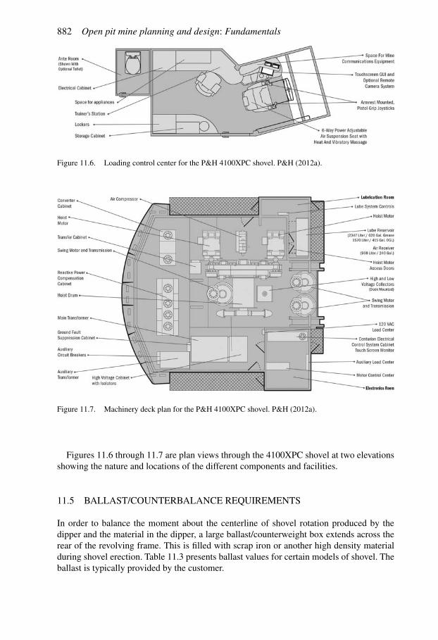
882 Open pit mine planning and design: Fundamentals
Figure 11.6. Loading control center for the P&H 4100XPC shovel. P&H (2012a).
Figure 11.7. Machinery deck plan for the P&H 4100XPC shovel. P&H (2012a).
Figures 11.6 through 11.7 are plan views through the 4100XPC shovel at two elevationsshowing the nature and locations of the different components and facilities.
11.5 BALLAST/COUNTERBALANCE REQUIREMENTS
In order to balance the moment about the centerline of shovel rotation produced by thedipper and the material in the dipper, a large ballast/counterweight box extends across therear of the revolving frame. This is filled with scrap iron or another high density materialduring shovel erection. Table 11.3 presents ballast values for certain models of shovel. Theballast is typically provided by the customer.

Shovel loading 883
Table 11.3. Ballast requirements for different standard shovel models (P&H (2012a,b,c,d)).
Make Model Nominal payload given by mfg Nominal dipper Ballast Ballastcapacity mt st
Metric tons (mt) Short tons (st)m3 yd3
P&H 1900AL 18 20 10.7 14 54.4 602300XPC 45.4 50 25.2 33 136.1 1502800XPC 59 65 33.6 44 230 253.54100XPC 109 120 61 80 204.1 225
The “nominal dipper capacity” values provided in the Table correspond to applying adensity of 1.78mt/m3 or 3000 lbs/yd3 to the given nominal payload.
11.6 SHOVEL PRODUCTION PER CYCLE
Prior to describing the shovel production calculation procedure, it is important to providesome definitions:
“Bank” versus “loose” properties.
In themine, thematerial which is to be loaded into the dippermust generally first be loosenedfrom its “in-place (in situ)” or “bank” position. In mining, this is often accomplished byblasting. Assuming that the material occupies a volume of 1 yd3 in place (denoted as 1 bankcubic yard, or 1 bcy), that same amount of material would be expected to occupy a largervolume in the loose condition. The weight of one cubic yard of loose material (one lcy),due to the presence of void (air) spaces between the pieces, would be less than the weightof one bcy. Values of the bank and loose weight densities for various materials are given inTable 11.4.
Swell:
The “swell” is defined as the ratio of the bank to loose weight densities.
Swell = bank weight/unit volume
loose weight/unit volume(11.1)
Percent swell:
The “percent swell” is defined as
Percent swell = 100(swell − 1) (11.2)
Swell factor:
The “swell factor” is the inverse of the swell
Swell factor = 1
swell= loose weight/unit volume
bank weight/unit volume(11.3)
The “swell factor” may also be expressed as
Swell factor = 100
(100 + percent swell)(11.4)

884 Open pit mine planning and design: Fundamentals
Table 11.4. Some properties for various materials which are important for loading machine evaluation.Atkinson (1971), Atkinson (1992).
Rock Specific Weight density Swell Percent Swell Fill Disabilitygravity swell factor ability(bank) lbs/bcy lbs/Icy (5%)
Asbestos ore 1.9 3200 2885 1.4 40 0.71 0.85 MBasalt 2.95 50000 3125 1.6 60 0.62 0.80 HBauxite 1.9 3200 2370 1.35 35 0.74 0.90 MChalk 1.85 3100 2384 1.3 30 0.76 0.90 MClay (dry) 1.4 2400 1920 1.25 25 0.80 0.85 MClay (light) 1.65 2800 2153 1.3 30 0.76 0.85 MClay (heavy) 2.1 3600 2666 1.35 35 0.74 0.80 M-HClay and gravel (dry) 1.5 2500 1923 1.3 30 0.76 0.85 MClay and gravel (wet) l.8 3000 2222 1.35 35 0.74 0.80 M-HCoal (anthracite) 1.6 2700 2000 1.35 35 0.74 0.9 MCoal (bituminous) 1.25 2100 1555 1.35 35 0.74 0.9 MCoal (lignite) 1.0 1700 1307 1.3 30 0.76 0.9 MCopper ore (low-grade) 2.55 4300 2866 1.5 50 0.66 0.85 M-HCopper ores (high-grade) 3.2 5400 3375 1.6 60 0.62 0.80 HEarth (dry) 1.65 2800 2153 1.3 30 0.76 0.95 EEarth (wet) 2.0 3400 2615 1.3 30 0.76 0.9 MGranite 2.41 4000 2580 1.55 55 0.64 0.8 HGravel (dry) 1.8 3000 2400 1.25 25 0.80 1.0 EGravel (wet) 2.1 3600 2880 1.25 25 0.80 1.0 EGypsum 2.8 4700 3133 1.5 50 0.66 0.85 M-HLimenite 3.2 5400 3857 1.4 40 0.71 0.85 MIron ore 40% Fe 2.65 4500 3214 1.4 40 0.71 0.8 M-HIron ore – 40% Fe 2.95 5000 3448 1.45 45 0.68 0.8 M-HIron ore – 60% Fe 3.85 6500 4193 1.55 55 0.64 0.75 HIron ore (taconite) 4.75 8000 4848 1.65 65 0.60 0.75 HLimestone (hard) 2.6 4400 2750 1.6 60 0.62 0.80 M-HLimestone (soft) 2.2 3700 2466 1.5 50 0.66 0.85 M-HManganese ore 3.1 5200 3586 1.45 45 0.68 0.85 M-HPhosphate rock 2.0 3400 2266 1.5 50 0.66 0.55 M-HSand (dry) 2.0 2900 2521 1.15 15 0.86 1.00 ESand (wet) 2.0 3400 2956 1.15 15 0.86 1.00 ESand and Gravel (dry) 1.95 3800 3304 1.15 15 0.86 1.00 ESandstone (pourous) 2.5 4200 2625 1.6 60 0.62 0.8 MSandstone (cemented) 2.65 4500 2812 1.6 60 0.62 0.8 M-HShales 2.35 4000 2758 1.45 45 0.68 0.8 M-H
An example of this type of calculation as applied to a copper ore is:
weight density (bank) = 3800 lbs/bcy
weight density (loose) = 2800 lbs/lcy
Swell = 3800
2800= 1.36
Percent swell = 100(1.36 − 1) = 36%
Swell factor = 1
1.36= 0.74

Shovel loading 885
Fillability or fill-factor
The “fillability” or the “fill-factor” is another factor which must be taken into account whenestimating production per cycle. This refers to the ratio of the loose volume of rock containedin the dipper to the rated dipper capacity.
fillability = loose volume of rock (yd3)
rated dipper capacity (yd3)(11.5)
Somecaremust be taken to assure that the “fillability” or the “fill-factors” and the rateddippercapacities go together. For shovels, the rated dipper capacity (nominal dipper capacity) isthe struck capacity. The “fillability” factors given in Table 11.4 apply to this volume. Ratedcapacities for front end loaders, for example, generally refer to a 2:1 heaped capacity andthe “fillability” factors based on this volume would be different from those given in Table11.4. In estimating fill factors, the following rules of thumb apply:
• a typical value is about 0.85 but higher values are sometimes quoted.• fill factors will be higher where the material is easy to dig and lower where digging ishard
• where material breaks finely, the fill factors will be higher• fill factors are higher for large equipment and lower for small equipmentThere are various ways of expressing the production per cycle. In mining, it is most
common to discuss tons. The basic equation may be written
Tc = Bc × Ff × WB × Sw (11.6)
whereTc = tons/cycleBc = nominal dipper capacity (yd3)Ff = fillability factorWB =weight density (lbs/bcy)Sw = swell factor
In civil construction, one is often more interested in the bank cubic yards moved percycle. In this case the expression may be written as,
Qc = Bc × Ff × Sw (11.7)
where
Qc = bank cubic yards/cycle
To obtain the production over a given time period, for example one shift, one needs to simplymultiply the production per cycle by the cycles in the time period.It is clear that the tons per cycle calculated using equation (11.6) must be compared to
the rated capacity for the shovel. If it is higher or lower than the rated, adjustments can bemade in
• dipper size• blasting patterns (to improve fragmentation).

886 Open pit mine planning and design: Fundamentals
11.7 CYCLE TIME
The average time (TA) required for a mining shovel to complete one cycle of• loading the dipper• hoisting and swinging• dumping• returning and lowering
is presented in Table 11.5 for different dipper volumes and digging conditions. These valuesare applicable for a swing angle of 90◦ and an optimum digging depth.As can be seen, Table 11.5 was developed for the shovels available at the time the initial
paper byAtkinson (1971) was written. For the modern loading shovels of today being usedin medium digging conditions, the cycle time is in the range of 33–35 seconds, basicallyindependent of dipper size (P&H, 2012e).For swing angles less than 90◦, the time required would be less. For angles greater than
90◦, it would be more. The modified cycle times can be estimated by application of a swingcorrection factor (CS) values for which are given in Table 11.6.With the inclusion of the angle of swing correction factor, the estimated cycle time
becomes
Tc = TACs
(11.8)
whereCs = swing correction factor from Table 11.6.
Table 11.5. Loading shovel cycle times (sec) assuming a 90◦ swing angle.Atkinson (1971).
Bc Digging conditions
yd3 m3 E M M-H H
4 3 18 23 28 325 4 20 25 29 336 5 21 26 30 347 5.5 21 26 30 348 6 22 27 31 3510 8 23 28 32 3612 9 24 29 32 3715 11.5 26 30 33 3820 15 27 32 35 4025 19 29 34 37 42
E. Easy digging. loose. free-running material, e.g. sand, small gravel. M. Medium digging,partially consolidated materials. e.g. clayey gravel, packed earth, clay, anthracite, tect.M-H Medium-hard digging, e.g. well blasted limestones, heavy wet clay, weaker ores,gravel with large boulders, etc. H. Hard digging-materials that require heavy blasting andtough plastic clays. e.g. granite, strong limestone, taconite strong ores, etc.
Table 11.6. Swing correction factor. Atkinson (1992).
Angle of swing, degrees 45 60 75 90 120 150 180Swing factor 1.2 1.1 1.05 1.00 0.91 0.84 0.77

Shovel loading 887
A second modifying factor to the cycle time concerns the vertical distance (depth of cutor cutting height) through which the dipper must move in order to be filled to capacity.Assuming an average bank penetration P, the vertical travel (L) required to fill a dipper
of width Wd and volume Bc is
L = Bc
WdP(11.9)
whereL= vertical travelBc = dipper volumeWd = dipper widthP= bank penetration
The depth of penetration depends upon the characteristics of the material being dug. InTable 11.5, the four categories; easy (E), medium (M), medium-hard (M-H), and hard (H)digging are used to classify the material. Since the filling portion (tf ) of the cycle time isrelated to L, the penetration would be high for easy digging materials and hence the neededcutting height would be low. On the other hand, for hard digging material the penetrationwould be low and hence the needed cutting height would be high.For a given dipper (Bc andWd fixed) operating in a given material (P fixed), there corre-
sponds an optimum depth of cut (Lo) which produces the greatest shovel output (tons/hour).For each pass the dipper comes up with a full load without undue crowding. The practicalapplication of this is that the bench height (H) should be greater than or equal to Lo toachieve the highest output.
H ≥ Lo (11.10)
SAE specification J732C specifies digging depth as
“the vertical distance in mm (inches) from the ground line to the bottom of thebucket cutting edge at the lowest position with the bucket cutting edge with thebucket cutting edge horizontal.”
A general rule of thumb that can be used is
“The optimum depth of cut is equal to the vertical distance from the dipper stickpivot shaft to the ground level.”
This position is shown in Figure 11.8.The relationship between optimum cutting height and dipper capacity shown in
Figure 11.9 can be expressed by either
Lo = 22 + Bc
3(11.11a)
or
Lo = 10.5 3√Bc (11.11b)
A second rule of thumb has been given by Martin (1982). They indicate that
“for good cutting, the penetration of the face should be uniform with a depthsufficient to fill the dipper in 2 or 3 dipper lengths”.

888 Open pit mine planning and design: Fundamentals
Figure 11.8. General working specifications of power shovels. (Ash, 1968).
Figure 11.9. Optimum cutting height as a function of dipper capacity.
Since the vertical distance from the dipper stick pivot to the ground is of the order of 2.5times the dipper length, the rules are fully consistent.When digging in bench heights less than Lo the cycle times must be multiplied by a bench
correction factor (CBH). Appropriate values are given in Table 11.7.

Shovel loading 889
Table 11.7. Correction factor for shovel cycle time as a function ofrelative digging depth. Atkinson (1971).
Optimum digging depth, percent 40 60 80 100Cycle time correction factor 1.25 1.10 1.02 1.0
It should be pointed out that the optimum cutting depth has nothing to do with themaximum cutting height of the shovel. This latter quantity is important in matching theshovel and the maximum bench height. In this regard the rule of thumb is
“themaximumbench height should be less than or equal to themaximum cuttingheight of the shovel.”
An alternate expression of this rule of thumb is that the digging face should not be higherthan the boom point sheave. This alternate form yields slightly higher values than that usingthe maximum cutting height (Fig. 11.8).The general formula for the expected cycle time can be written as
Tc = TA × CBH
Cs(11.12)
whereTc = cycle timeTA = average cycle time (90◦) for an optimum or greater digging depthCs = swing correction factorCBH = bench height correction factor
11.8 CYCLES PER SHIFT
Now that the time to perform one shovel cycle has been determined, it is possible to calculatethat which is really desired, the cycles per shift. With this information and the load per cycleone can calculate the production per shovel shift. It will be assumed that the length of theshift (T ) is
T = 3600 H (11.13)
whereT = shift length (sec)H = shift length (hrs)
The theoretical number of cycles which could be performed is
CTheoretical = 3600H
Tc(11.14)
In fact, the length of time that the shovel is actually cycling, is much less than 3600H.When examining the shift production from a shovel it is important to distinguish between
cycling time and clock (shift) time. Cycling time is that portion of the shift when the shovelis rotating between bank and truck. Clock time is the total time that an operator or crew is

890 Open pit mine planning and design: Fundamentals
Table 11.8. Propel factor. Atkinson (1971).
Strip mines 0.75Multi-bench mines 0.85Sand and gravel pits 0.90High-face quarries 0.95
assigned to the machine. For an eight hour shift the value would be 8 hours or 480 minutes.The cycling time would be less than the clock time due to
• Mechanical availability (less than 100% machine availability during thescheduled shift).
• Job operational factors (less than 100% utilization of the available time).• Propel time (time required to maneuver the shovel to the next loading position)
Included under the general heading of job operational factors are such things as:• travel to and from the working place• lunch time• lubrication and fueling time• waiting time• time lost due to weather conditions, spent in safety meetings, etc.The time required to propel the shovel during maneuvering is sometimes included as
one of the job operational factors. Here it will be kept separate. For this discussion themechanical availability factor (MA) will be defined as
MA = clock time − down time
clock time(11.15)
The available time (TA) then becomes
TA = clock time − down time (11.16)
The utilization factor (UA) is defined as
UA = cycling time
available time(11.17)
The job efficiency factor (E) is the product of the mechanical availability and utilizationfactors
E = MA × UA (11.18)
As indicated, a portion of the total time is spent moving the shovel into position (propelling).Propel factors (P) are given in Table 11.8 for various types of operations.Table 11.9 is a portion of a shovel shift summary report from a large open pit copper mine
for which the clock time is 480 minutes.Themechanical availability, utilization and job efficiency factors for each of these shovels
for this shift is given in Table 11.10.

Shovel loading 891
Table 11.9. Shovel shift report.
A Shift 15-Mar-82 at 15:50:15
Shovel Operator name Idle Down Delay T&L Spare(min) (min) (min) (min) (min)
9 MARQUEZ, R.M. 88. 0. 32. 45. 0.10 SMITH, L.W. 165. 0. 0. 50. 11.11 MARTINEZ, F.M. 33. 0. 6. 50. 11.12 FLORES, O.T. 70. 71. 5. 50. 15.13 WOOD, R.G. 31. 208. 0. 30. 16.
Table 11.10. Mechanical availability, utilization and job efficiency from Table 11.9.
Shovel Mechanical Utilization Job efficiencyavailability
9 1.00 0.66 0.6610 1.00 0.53 0.5311 1.00 0.79 0.7912 0.85 0.66 0.5613 0.57 0.72 0.41Average 0.88 0.67 0.69
A total of 1415 minutes was spent cycling out of the possible 2400 minutes clocktime bythe 5 shovels. The average factors were:
Mechanical availability = 0.88
Utilization = 0.67
Job Efficiency = 0.59
For an actual operation it is important to examine such figures to see where improvementsmight be made. In this case the utilization is quite low due in large part to time spent waitingfor trucks. Shovel productivity improvements could be achieved by the assignment of moretrucks.The average number of cycling minutes (M) to be expected during a shovel shift can be
calculated using
M = clock time (minutes) × MA × UA × P (11.19)
or
M = clock time (minutes) × E × P (11.20)
For the case examined in Tables 11.8 and 11.9 (assuming P= 1 since it is not reported) onewould find for a single shovel that
M = 480 × 0.88 × 0.67 = 283 minutes
or
M = 480 × 0.59 = 283 minutes

892 Open pit mine planning and design: Fundamentals
Table 11.11. Time distribution for average delays per hour expressed in minutes and % for a shoveloperation. Church (1981).
Time distributionDelays to shovel operation min %
Minor delays of less than 15min duration:Insufficient rock haulers 4.2 7.0Spotting of rock haulers at shovel 1.0 1.7Shovel moves at face of cut 1.4 2.3Shovel repairs and maintenance 1.4 2.3Shovel handling of outsize rocks and stumps 0.7 1.2Checking grade 0.3 0.5Shovel operator’s and other delays 0.8 1.3Subtotals 9.8 16.3
Major delays of more than 15 min durationMoving to next cut and opening up cut 2.4 4.0Shovel repairs and maintenance 3.0 5.0Subtotals 5.4 9.0
All minor and major delays, totals 15.2 25.3
For the five shovels operating during the shift, the total is 1415 minutes or very close to theactual value as would, of course, be expected.From an estimating viewpoint there are some guidelines from the literature regarding
values of MA, UA and E.Crawford (1979) states that electric shovels can normally sustain 75 to 80% availability
and 80 to 90% utilization of availability for a substantial portion of their nominal 20-yearlife. The corresponding values would be
MA = 0.75 to 0.80
UA = 0.80 to 0.90
E = 0.60 to 0.72
As a rule of thumb, Crawford (1979) indicates
“Allowing for minimum delays, an attainable target shovel productivityapproaches 1185 t/dipper m3 (1000 st/dipper yd3) per 8 hour shift. The ruledoes not apply to coal or other light weight materials.”
Steidle (1977) in his rules of thumb for mining shovels suggests
MA = 0.70 to 0.80 (diesel)
MA = 0.90 (electric)
UA = 0.83
Church (1981) has presented the delay data (Table 11.11) in the operating cycle for shovelearth-rock production.As can be seen the average hourly delays (clock time) have been split into (a) minor delays
of less than 15min. duration and (b) major delays of more than 15min. duration. Repair aswell as operating delays are lumped together.

Shovel loading 893
11.9 SHOVEL PRODUCTIVITY EXAMPLE
To practice the concepts, calculate the production (bank volume per hour) from a shovel forwhich the following conditions apply:
• Dipper capacity (volume)= 15 yd3
• Swing angle= 120◦ (time for a 90◦ swing is 30 sec.)• Mechanical availability= 95%• Working time= 50min/hr.• Optimum digging depth= 100% of optimum• Swell= 30%• Fill factor (fillability)= 90%• Multi-bench mine• Ore S.G.= 2.7The calculation process will now be demonstrated:
Cycles/hour:
C = theoretical cycles/hr = 60min/hr
0.5min/cy= 120 cy/hr
CBH = 1.0
CS = swing correction (120◦ rather than 90◦), therefore CS = 1.10
Thus, the corrected cycles= 120/1.1= 109.09 cy/hr.
A = 0.95 Availability
O = 50/60 = 0.83 working time
Thus, corrected cycles= 109.09× 0.95× 0.83= 86
P = propel = 0.85
Thus, actual cycles= 0.85× 86= 73.12 cy/hr.
Material/Cycle
Qc = Bc × Ff × Sw
Bc = 15 yd3 = dipper capacity (yd3) − “loose”
Ff = fill factor (expressed as a ratio) = 0.90
Thus, material/cycle (loose)= 15× 0.90= 13.50 yd3/cyBut the material has broken and swelled.
% Swell = 30%
Sw = 100
100 + %Swell= 100
100 + 30= 0.769
Thus,
Material/cycle (bank − solid) = 13.50/1.30 = 12.38 yd3

894 Open pit mine planning and design: Fundamentals
Bank Volume/Hr
Cycles/hr × bank material/cycle = 73.12 × 12.38
= 759 bank yd3/hr
Tons/hr
Tons/yd3 = 2.7 × 62.4 × 27
2000= 4949
2000= 2.27 tons/yd3
Tons/hr = 759 × 2.27 = 1723 tons/hr.
Tons/Shift= 8 hrs/shift× 1723 tons/hr= 13784 tons/shift for 15 yd3 shovel.Rule of Thumb= 1000 tons/yd3 dipper capacity/8-hour shift.In this case,
13784/15 = 919 tons/yd3 dipper capacity/shift
which is similar to the rule-of-thumb value.
11.10 DESIGN GUIDANCE FROM REGULATIONS
For a safe and efficient shovel-truck loading operation it is important that the geometriesinvolved are well matched. Some design guidance is provided by regulation some of whichare paraphrased below:
• Standards for the safe control of pit walls, including the overall slope of the pit wall,shall be established and followed by the operator. Such standards shall be consistentwith prudent engineering design, the nature of the ground and the kind of material andmineral mined, and the ensuring of safe working conditions according to the degreeof slope. Mining methods shall be selected which will ensure wall and bank stability,including benching as necessary to obtain a safe overall slope.
• To ensure safe operation, the width and height of benches shall be governed by typeof equipment to be used and the operation to be performed.
• Safe means for scaling pit banks shall be provided. Hazardous banks shall be scaledbefore other work is performed in the hazardous bank area.
• Men shall not work near or under dangerous banks. Overhanging banks shall be takendown immediately and other unsafe ground conditions shall be corrected promptly, orthe areas shall be barricaded and posted.
• Berms or guards shall be provided on the outer bank of elevated roadways.• Dippers, buckets, loading booms, or heavy suspended loads shall not be swung overthe cabs of haulage vehicles until the drivers are out of the cabs and in safe locations,unless the trucks are designed specifically to protect the drivers from falling material.
• Haulage equipment shall be loaded in a manner to minimize spillage during haulage.The requirement for providing a safe means for scaling pit banks impacts the choice of
equipment and the bench heights.Although some special pieces of equipment and techniqueshave and are being used to scale the pit walls, it is most common to do this with the primaryexcavator. For a loading shovel, this means that the bench height should be less than orequal to the maximum cutting height (hm) of the shovel.

Shovel loading 895
REFERENCESAND BIBLIOGRAPHY
Aksoy, C.O. 2005. Minimizing the economic unit cost of dragline-truck-shovel operations at Yatagan-Eskihisar open pit mine, Turkey. CIM Magazine. June/July. pp. 331–334.
Aksoy, C.O., Kose, H., Malli, T., Ozfirat, K., Gonen, A., & S. Gurgen. 2005. Truck-shovel optimizationaccounting for cost, safety, and operational practice. CIM Magazine. November. pp. 402–406.
Anonymous. 2007. Equipment – Buckets: Bucket basics. Mining Magazine. February. pp. 43–48.Anonymous. 2007. Management in action – Excavator selection: Electric versus hydraulic. Mining
Magazine. April. pp. 42–51.Anonymous. 2009. Equipment – Rope shovels: Shovel shake-ups. Mining Magazine. April. pp. 27–29.Anonymous. 2010. Equipment – Rope shovels: Super shovels. Mining Magazine. April. pp. 40–44.Anonymous. 2010. News – Caterpillar to buy Bucyrus. Mining Magazine. December. p. 2.Anonymous. 2011. Surface loaders – fully loaded. Mining Magazine. April. pp. 38–45.Ash, R.L. 1968. Chapter 7.3 The design of blasting rounds. In Surface Mining (E.P. Pfleider, editor). AIME,
NY. pp. 373–397.Atkinson, T. 1971. Selection of open pit excavating and loading equipment. Institution of Min. & Met.
Trans. Section A. London. July. pp. A101–A129.Atkinson, T. 1992. Chapter 13.3 Selection and sizing of excavating equipment. In SMEMining Engineering
Handbook, 2nd Edition, Vol. 2 (H.L. Hartman, editor). SME. Baltimore, Maryland. pp. 1311–1333.Awuah-Offei, K., Osei, B., & H. Askari-Nasab. 2012. Improving truck-shovel energy efficiency through
discrete event modeling. 2 Paper 12-069. SMEAnnual Meeting. Feb 19–22. Seattle, WA.Bastock, M., & P. Knights. 2009.Applying modular transporters to relocate large hydraulic excavators. Iron
Ore 2009 Conference. Perth, WA. July 27–29. pp. 217–222.Berkhimer, E.N. 2011. Chapter 10.4 Selection and sizing of excavating, loading, and hauling equipment.
In SME Mining Engineering Handbook, 3rd Edition (P. Darling, editor). pp. 931–939.Bogunovic, D., & V. Kecojevic. 2011. Impact of bucket fill factor on dragline production rate and energy
consumption. Mining Engineering. 63(8): 48–53. August.Carter, R.A. 2005. Mining with precision: The latest generation of global positioning system (GPS) and
geographic information system (GIS) technologies offers unprecedented accuracy for earthmoving andmapping. E/MJ. 206(4): 42–46. May.
Carter, R.A. 2006. Giving new life to old shovels. E/MJ. 207(7): 40–42. September.Carter, R.A. 2007. Digital diggers: When it comes to digging and loading efficiency, equipment size may
not always be the supreme factor. E/MJ. 208(1): 34–38. January/February.Carter, R.A. 2008. GET smart: Ground engaging tools (GET) are designed to make the ultimate sacrifice –
offering their service lives to promote better penetration and protect vulnerable bucket areas. E/MJ.209(2): 58–60. March.
Carter, R.A. 2008. Hydraulic excavator overhauls – when and what to plan for. E/MJ. 209(3): 50–52. April.Carter, R.A. 2010. Tracking new developments in dozer design. E/MJ. 211(2): 30–32. March.Carter, R.A. 2010. New wheel loaders roll ahead to higher reliability, improved productivity. E/MJ. 211(6):
64–67. July/August.Chanda, E.K., & R.J. Hardy. 2011. Selection criteria for open pit production equipment – Payload distribu-
tions and the ‘10/10/20’policy. Proceedings of the 35thAPCOM.WollongongNSW,Australia. September24–30. pp. 351–364.
Church, H.K. 1981. Excavation Handbook. McGraw-Hill Book Company, NewYork. pp. 12-21 to 12-32. lInstitution of Min. & Met. Trans. Section A. London. July. pp. A101–A129.
Crawford, J.T., III. 1979. Section 19. Shovel and haulage truck evaluation. Open Pit Mine Planning andDesign (J.T. Crawford, III and W.A. Hustrulid, editors). AIME. pp. 258–270.
Dessureault, S., Yildirim, M., & M. Baker. 2007. Data mining mine data: truck-shovel fleet managementsystems. CIM Magazine. June/July. pp. 134–142.
Ercelebi, S.G., & A. Bascetin. 2009. Optimization of shovel-truck system for surface mining. JSAIMM.109(7): 433–439.
Fiscor, S. 2005. Optimized dippers fine-tune shovel performance. E/MJ. 206(7): 76–79. September.Fiscor, S. 2007. Productivity considerations for shovels and excavators. E/MJ. 208(7): 38–42. September.Fiscor, S. 2009. Smarter shovels dig and load more efficiently. E/MJ. 210(3): 44–47. April.Fiscor, S. 2010. Shovel OEMs make major design improvements. E/MJ. 211(7): 76–81. September.

896 Open pit mine planning and design: Fundamentals
Frimpong, S., & O. Brown. 2011. Optimization of shovel dipper – formation interactions in excavation.Paper 11-100. SMEAnnual Meeting. Feb 27–Mar 2. Denver, CO.
Frimpong, S., & Y. Hu. 2005. Dynamic hydraulic shovel simulator for improved machine performance.CIM Magazine. January/February. pp. 155–159.
Frimpong, S., & Y. Li. 2006. Real-time monitoring of cable shovel stress for improved machine health.Paper 06-039. SMEAnnual Meeting. Mar 26–29. St. Louis, MO.
Frimpong, S., &Y.Li. 2007. Cable shovel health and longevity in formation excavation.MiningEngineering.59(12): 50–56. December.
Frimpong, S., Hu, Y., & J. Szymanski. 2003. Intelligent cable shovel excavation in surface mining. Paper03-37. SMEAnnual Meeting. Feb 24–26. Cincinnati, OH.
Hansen, J. 2001. Electric rope shovel monitoring. Paper 01-104. SME Annual Meeting. Feb 26–28.Denver, CO.
Harcus, M. 2011. LeTourneau update – born in the USA. Mining Magazine. January/February. pp. 9–10.Haut, H., & M. Dietrich. 2011. A multibody simulation solution to analyse attachment kinematics of
hydraulic excavators and other linkages. Proceedings of the 35th APCOM.Wollongong NSW,Australia.September 24–30. pp. 679–687.
Humphrey, J.D., & J. D. Wagner. 2011. Chapter 10.3 Mechanical extraction, loading, and hauling. In SMEMining Engineering Handbook, 3rd Edition (P. Darling, editor). pp. 903–929.
Joseph, T.G., & N. Shi. 2011. Scale field tests and visual modeling to evaluate a curved front dipper concept.CIM Journal. 2(3): 125–134.
Joseph, T.G., & N. Shi. 2011. Scaling analysis via geometric and performance data for shovel dipper design.CIM Journal. 2(4): 171–177.
Joseph, T.G., & N. Shi. 2011. Simulation of cable shovels and dippers in mining applications. CIM Journal.2(3): 135–142.
Joseph, T.G., & N. Shi. 2012. A revised dipper-ground equilibrium derivation for shovels operating in oil,sand, and soft ground. CIM Journal. 3(1): 47–53.
Kirmanli, C. & S.G. Ercelebi. 2009. An expert system for hydraulic excavator and truck selection in surfacemining. JSAIMM. 109(3): 727–738.
Komatsu. 2009. Komatsu Specifications and Application Handbook. Edition 30.Li, Y., & S. Chang. 2009. The modeling and simulation of Bucyrus shovel, Part 1: Spacial kinematics and
virtual prototype modeling. Paper 09-122. SMEAnnual Meeting. Feb 22–25. Denver, CO.Li, Y., Liu, W., Shi, X., & S. Frimpong. 2009. Cable shovel dynamic modeling for determining component
cycle stress. Paper 09-121. SMEAnnual Meeting. Feb 22–25. Denver, CO.Lucio, J.C., Senra, C.T., & A. Souza. 2009. Paving the future – A case study replacing truck-and-shovels
by shovel-and-conveyor continuous mining at Carajas open pit mines. Iron Ore 2009 Conference. Perth,WA. July 27–29. pp. 269–276.
Martin, J.W., T.J. Martin, T.P. Bennett, & K.M. Martin. 1982. Surface Mining Equipment. MartinConsultants, Golden, CO. 455 pp.
Mkhatshwa, S.V. 2009. Optimization of the loading and hauling fleet at Mamatwan open pit mine. 109(4):223–232.
Moore, P. 2006. Equipment – Surface loaders: The essence of excavators. Mining Magazine. August.pp. 15–21.
Moore, P. 2008. Equipment – Large wheel loaders: Big wheels keep on turning. Mining Magazine. June.pp. 26–31.
Moore, P. 2010. Equipment access – Access all areas. Mining Magazine. December. pp. 30–33.Norrena, K., &C.V.Deutsch. 2001.Automatic determination of dig limits subject to geostatistical, economic
and equipment constraints. Paper 01-41. SMEAnnual Meeting. Feb 26–28. Denver, CO.Oraee, B., Lashgari, A., & A. Sayadi. 2011. Estimation of capital and operation costs of backhoe loaders.
Paper 11-040. SMEAnnual Meeting. Feb 27–Mar 2. Denver, CO.P&H. 2012a. P&H 4100XPC Digital AC Drive Electric Mining Shovel.P&H. 2012b. P&H 2800XPC Digital AC Drive Electric Mining Shovel.P&H. 2012c. P&H 2300XPC Digital DC Drive Electric Mining Shovel.P&H. 2012d. P&H 1900AL Electric Mining Shovel.P&H. 2012e. Personal communication. June–July.Porter, D. 2006. Equipment – Surface load-haul: Riding on a super cycle. Mining Magazine. April.
pp. 11–17.

Shovel loading 897
Porter, D. 2006. Opinion – Equipment trends: Payload weighing: In search of the Grail. Mining Magazine.August. pp. 22–23.
Porter, D. 2008. Disciplined digging – P&H C-series. Mining Magazine. February. pp. 26–30.Porter, D. 2010. P&H Prevail – Advances in remote health monitoring. Mining Magazine. November.
pp. 16–19.Rathmann, B., & U. Heuer. 2007. Refit of an electric shovel or dragline – a cost saving alternative between
frequent repairs and the purchase of a new machine. Paper 07-026. SME Annual Meeting. Feb 25–28.Denver, CO.
Raza, M., & S. Frimpong. 2011. Cable-shovel dipper mechanics. Paper 11-096. SME Annual Meeting.Feb 27–Mar 2. Denver, CO.
Rogers, B. 2007. Equipment – Large wheel loaders: Wheeled versatility adds value. Mining Magazine.April. pp. 52–55.
Roos, C., Conrad, P. & S. Rosenthal. 2009. Estimating excavator teeth consumption rates. Paper 09-021.SMEAnnual Meeting. Feb 22–25. Denver, CO.
Roos, C.J., Conrad, P.W., & S.D. Rosenthal. 2010. Estimating excavator teeth consumption rates. MiningEngineering. 62(8): 45–51. August.
Saavedra, P.N., & C.J. Molina Vicuña. 2007. Online monitoring for mining shovels focused on vibrationanalysis. CIM Magazine. May. pp. 101–110.
Sargent, F.R. 1990. Section 6.4 Loading. pp. 620–657. Surface Mining, 2nd Edition (B.A. Kennedy, editor).SME.
Segarra, P., Sanchidrian, J.A., Montoro, J.J., & L.M. López. 2007. Mucking efficiency in open pit blasting.CIM Magazine. September/October. pp. 246–256.
Shi, N., & T.G. Joseph. 2006. A new Canadian shovel dipper design for improved performance. CIMMagazine. March/April. pp. 99–104.
Singh, S.P., & R. Narendrula. 2006. Productivity indicators for loading equipment. CIM Magazine. May.pp. 125–132.
Steidle, E.J. 1977. Evaluation of draglines and shovels in mining. Min. Cong. J. April. pp. 30–33.Turnbull, D., & A Cooper. 2009. In-pit crushing and conveying (IPCC) – A tried and tested alternative to
trucks. The AusIMM 2009 New Leaders Conference. Brisbane QLD. April 29–30. pp. 59–66.Turnbull, D., & A. Cooper. 2010. In-pit crushing and conveying (IPCC) – A tried and tested alternative to
trucks. Part 1. AusIMM Journal. Issue 5. Oct.Turnbull, D., & A. Cooper. 2010. In-pit crushing and conveying (IPCC) – A tried and tested alternative to
trucks. Part 2. AusIMM Journal. Issue 6. Dec.Woof, M. 2005. A boom market for excavators. E/MJ. 206(5): 50–52. June.Yavuz, M. 2008. An application of the TOPSIS method to solve hydraulic excavator selection problem in
mining. Paper 08-042. SMEAnnual Meeting. Feb 24–27. SLC, UT.
ACKNOWLEDGEMENTS
The authors would like to acknowledge the assistance provided by Joy Global in preparingthis chapter. Thomas Martin has generously allowed us to include information from thebook “Surface Mining Equipment” written by J.W. Martin, T.J. Martin, T.P. Bennett, andK.M. Martin. It must be clearly stated that any misinterpretation of source information andmistakes in understanding are clearly the responsibility of the authors.
REVIEW QUESTIONSAND EXERCISES
1. The chapter is focused entirely on “rope” shovels. Hydraulic shovels and wheel loadersplay an important part in modern mining operations. The reader is encouraged to con-struct a table showing the primary operating regime for rope shovels, hydraulic shovelsand wheel loaders.

898 Open pit mine planning and design: Fundamentals
2. Given figure 11.1 with the various parts numbered, be able to supply the labels.3. Describe the digging action of a modern shovel. Try to include as much of the “physics”
in your discussion as possible.4. Examine the digging profile in Figure 11.3. How does this relate to the final bench
face angles observed in open pit mines? Is it easy to achieve vertical faces? Why orwhy not?
5. In Figure 11.3, it is seen that the maximum digging height is about equal to the heightof the sheave wheel. If the shovel is used to scale the bench faces and make them safe,what design rule would emerge?
6. Assume that the geomechanics department has specified certain bench face angles intheir pit slope designs. How easy is it to construct them in practice using typical shovelpractices?
7. With regard to question 6, review Figure 11.4. Assume that via a computer I can controlthe hoist, crowd and propel all at the same time. Would I now be able to constructthe bench angles as specified by geomechanics? Why or why not? Make a drawing insupport of your thinking.
8. Martin (1982) has presented a rather long list of “operational practices.” Review thelist and identify five which you deem to be the most important.
9. Turn your attention to Figure 11.1. Note the position of the dipper and the ballast box.Construct a simple free-body diagram representing the loaded shovel. If you were theshovel designer, would you specify the dipper capacity by volume or by weight?Why?
10. In continuing the thinking process of problem 9, what modifications can you makewhen loading materials of different densities? Think about loading coal versus loadingiron ore.
11. What is meant by struck capacity? What is meant by heaped capacity? What controlshow full the dipper is actually filled?
12. In the past, it was quite common to quote dipper capacity in terms of volume with theassumptions that the material had a nominal weight of 3000 lb/yd3 and the struck capac-ity applied. Review the specification sheets for the shovels of various manufacturersand see how well this applies.
13. Some of the dimensions for the P&H 4100XPC electric rope shovel are provided in Fig-ure 11.5 and Table 11.1. If the bench height should be matched to the maximum cuttingheight, what would that be? What would it be if the sheave height is used instead?
14. For the P&H 4100XPC shovel, what is the dumping height? How is this dimensionconsidered in practice?
15. What is the significance of the “Radius of the level floor” dimension?16. The angle between the dipper stick and the dipper is typically 65 degrees. Why is this
a logical choice?17. A cross-section through the P&H 4100XPC shovel is shown in Figure 11.5. From a
dimension point of view, how does this shovel compare to the competitors? What aretheir respective capacities?
18. Some of the dimensions for the P&H shovel line are summarized in Tables 11.1 and11.2. Are there some dimensions which you think should be added to the tables?
19. Figures 11.6, 11.7 and 11.8 show the arrangement of the different pieces of equipment,the facilities and the operating accommodations on the 4100XPC shovel. The operatorseems to have all the comforts of home and then some. Summarize these.

Shovel loading 899
20. Using the ballast and payload numbers provided inTable 11.3, perform a simplemomentbalance for the 4100XPC shovel. What is your conclusion?
21. Define the following terms:– Bank weight– Loose weight– Swell– Percent swell– Swell factor– Fillability– Fill factor
22. Can you think of a practical way to get a handle on the fillability factor?23. Often unit operations are considered as separate entities or even “kingdoms.” But there
is a very clear connection between the fragmentation achieved and the efficiency of theloading operation. How would one optimize the process, that is, when is it of interestto spend extra resources on the fragmentation?
24. Material has been classified as easy digging, medium digging, medium-hard diggingand hard digging. How is this distinction being made? How would you do it?
25. A curve relating the optimum cutting height to the dipper capacity has been preparedbased on earlier models of loading machines. Does this curve also represent the newmodels presented in this chapter?
26. Check the old rule-of-thumb that for good cutting the dipper should fill in a cutting heightof 2 to 3 dipper lengths, i.e. compare the dipper stick pivot position to the approximatedipper length.
27. Carefully review and understand the calculations and input data leading to the estimationof production per shift.
28. An old rule-of-thumb is that during an 8-hr shift a shovel should load 1000 shorttons/cubic yard of dipper capacity. Hence for the P&H 4100XPC shovel equippedwith an 82 yd3 dipper, one would expect it to load 82,000 tons over an 8-hr shift. Perusethe mining literature and/or check with mining operations to determine the applicabilitytoday.
29. Wheel loaders are often used both as primary and secondary excavators in mining oper-ations today. One problem is that they do not have the same digging height capability asrope shovels and thus have problems in scaling bench faces. How is this to be overcome?
30. If one applies the rule that a shovel should fill a truck to capacity in 3 to 5 swings, whatsize trucks should be assigned to the P&H line of shovels?
31. How is shovel capacity influenced by the number of trucks assigned to the shovel, theloading time and the haul time?

CHAPTER 12
Haulage trucks
12.1 INTRODUCTION
Over the years off-highway trucks have established themselves as the primary means bywhich both ore and waste are moved in large open pit mines. Because haulage costs can beas much as 50 percent of the total operating costs at a given mine, it is imperative that athorough understanding of haulage in general, but particularly truck haulage, be achieved.This chapter will focus on some selected aspects of trucks needed by mining engineers inestimating truck requirements, production capacities and costs. In particular, the followingtopics will be discussed in some detail.a. Sizing the container.b. Powering the containerc. Propelling the container: Principles of mechanical and electric drive systems.d. Estimation of cycle timese. Calculation of production rates.There are many other factors which enter into the selection of a haulage system. Unfortu-
nately they cannot be covered here. Although somewhat dated, the reader is encouraged toread the excellent series of articles on the subject written by Burton (1975a, 1975b, 1975c,1975d, 1976).
12.2 SIZING THE CONTAINER
A haulage truck is in simplest terms, a container (the body) on drive wheels. Generallythe overall haulage objective is to accomplish the movement of material from one point toanother with the lowest possible cost. The amount of material moved per cycle dependsupon the size of the container used. The time required over a given route depends upon thecharacteristics of the driving mechanism (prime mover, drive train, wheels, tires, etc.). Inthis section, the characteristics of the container will be examined. The following section willdeal with the driving mechanism. The haulage truck is but one element in the transportationchain stretching from the broken material in the pit to the final destination, be it the primarycrusher or the dump.A basic consideration is that the loading and hauling equipment shouldbe matched.Clearly for a given shovel (loader) production capacity (tons/hour) one could assign to
the shovel (a) a few large capacity trucks requiring a high number of fill cycles or (b) manysmall capacity trucks requiring a few fill cycles. The correct “match” obviously depends
900

Haulage trucks 901
Table 12.1. Example truck specification.
Payload= 170 tons (340,000 lbs)Load Capacity (Volume) (yd3) (m3)
Struck (SAE) 89.5 68.4Heap 3:1 115.1 87.9Heap 2:1 (SAE) 126.9 97.0
Table 12.2. Slope angle and angle of repose for various materials (InternationalPayline Division, 1975).
Material Slope in repose Angle of repose (degrees)
Bauxite 1.0:1 45Clay, dry 2.0:1 27Clay, light 2.0:1 27Clay, wet 1.0:1 45Coal, anthracite 1.2:1 40Coal, bituminous 1.2:1 40Copper ore 1.0:1 45Earth, dry 2.0:1 27Earth, moist 1.0:1 45Earth, wet 2.0:1 27Gravel, dry 2.0:1 27Gravel, wet 2.0:1 27Granite 1.0:1 45Iron ore, hematite 1.0:1 45Limestone, blasted 2.0:1 27Rock & stone, crushed 2.0:1 27Sand, dry 3.0:1 18Sand, wet 2.0:1 27Shale, soft rock 1.0:1 45Slate 1.0:1 45Trap rock 1.0:1 45
upon a number of criteria some of which are site specific. A general rule-of-thumb used inmining is that 3 to 5 shovel swings should be used to fill the truck to capacity.The meaning of truck capacity is important. If one examines truck specification sheets,
one will see a variety of terms being presented. Table 12.1 shows an example of this. Thetruck in this case is equipped with the standard body.Standards regarding the calculation of truck and heaped capacity are set by the Society
of Automotive Engineers (SAE). The struck capacity is how much water the truck bodywould hold if brim full. The heaped capacity is the amount of additional material that can beplaced above the sides of the container.A slope of 1:1 rises one vertical unit in one horizontal.Different broken materials stand at different slope angles. These angles are referred to asthe angle of repose. Values for different materials are given in Table 12.2.The reason that both volume and weight must be considered is that the loading machine
places a certain volume of rock into the truck each swing.A general rule-of-thumb which is often applied to the sizing of haulage units is the
assumption that 1 yd3 of broken material weighs 3000 lbs. In applying this factor to thebody sizes listed in Table 12.1, one obtains the values in Table 12.3.

902 Open pit mine planning and design: Fundamentals
Table 12.3. Tonnage values corresponding to the volumes in Table 12.1.
Volume Notation Volume (yd3) Tons
Struck (SAE) 89.5 134Heap 3:1 115.1 173Heap 2:1 (SAE) 126.9 190
For this standard body and this material, the tonnage capacity is matched by a 3:1 heapedload (115.1 yd3). If the dipper capacity is 23 yd3/swing, the truck could be filled to capacityin 5 swings. The concept of swell and swell factors has been discussed in some detail in theloading section. The same principles apply here.For materials having densities less than 3000 lbs/yd3, to achieve the rated payload
capacity• either a greater heap would be required,• or a larger body size should be ordered.For materials having densities greater than 3000 lbs/yd3, the rated payload would be
achieved by utilizing only a portion of its heaped/struck capacity or a smaller truck bodycould be ordered. Overfilled trucks result in spillage costs, higher tire cost, higher truckmain-tenance cost. Under-filled trucks also result in higher costs/ton hauled. Therefore a thoroughevaluation of truck capacity within the overall material transport chain must be made.
12.3 POWERING THE CONTAINER
Vehicle motion is achieved by applying a force parallel to the road surface by the rim (outeredge) of the tire. This force which is called the rimpull (RP) or tractive effort (TE) is shownin Figure 12.1.The radius through which the force is applied is the rolling radius (RR) or static loaded
radius of the tire. Hence the wheel torque (WT) required is
WT = RP × RR (12.1)
whereWT =wheel torqueRP= rimpullRR= rolling radiusFor a large haulage truck equipped with 27.00–49 tires, the rolling radius is 51.6 ins
(4.3 ft). If, in starting from rest, the required rimpull is 15,000 lbs, the wheel torque wouldbe 64500 ft-lbs. The rotary power required to rotate thewheel at nwheel rotations perminute is
W = 2πnwheelWT
33000(12.2)
whereW= required rotary power (HP)nwheel =wheel rotation rate (RPM)WT =wheel torque (ft-lbs)33000= factor required to convert ft-lbs/minute to horsepower.
UFM
|484
942|
1435
6129
76
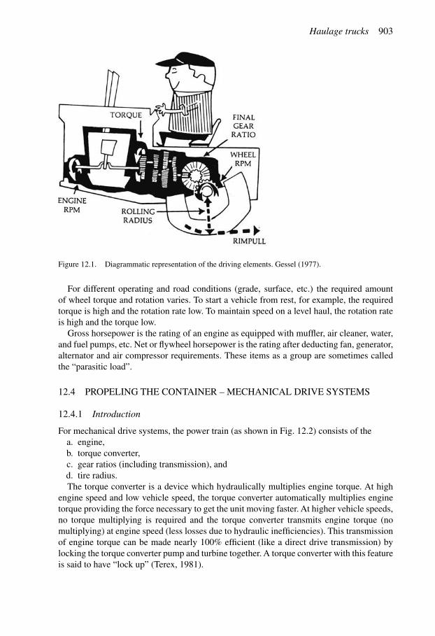
Haulage trucks 903
Figure 12.1. Diagrammatic representation of the driving elements. Gessel (1977).
For different operating and road conditions (grade, surface, etc.) the required amountof wheel torque and rotation varies. To start a vehicle from rest, for example, the requiredtorque is high and the rotation rate low. To maintain speed on a level haul, the rotation rateis high and the torque low.Gross horsepower is the rating of an engine as equipped with muffler, air cleaner, water,
and fuel pumps, etc. Net or flywheel horsepower is the rating after deducting fan, generator,alternator and air compressor requirements. These items as a group are sometimes calledthe “parasitic load”.
12.4 PROPELING THE CONTAINER – MECHANICAL DRIVE SYSTEMS
12.4.1 Introduction
For mechanical drive systems, the power train (as shown in Fig. 12.2) consists of thea. engine,b. torque converter,c. gear ratios (including transmission), andd. tire radius.The torque converter is a device which hydraulically multiplies engine torque. At high
engine speed and low vehicle speed, the torque converter automatically multiplies enginetorque providing the force necessary to get the unit moving faster. At higher vehicle speeds,no torque multiplying is required and the torque converter transmits engine torque (nomultiplying) at engine speed (less losses due to hydraulic inefficiencies). This transmissionof engine torque can be made nearly 100% efficient (like a direct drive transmission) bylocking the torque converter pump and turbine together. A torque converter with this featureis said to have “lock up” (Terex, 1981).

904 Open pit mine planning and design: Fundamentals
Figure 12.2. Power train of a mechanical drive system. Terex (1981).
Figure 12.3. The Terex 33-09 truck. Terex (1974).
Gear ratios provide an increase in the torque and a resultant reduction in speed. The totalgear reduction (TGR) is a multiple of all the gear ratios which make up the gear train;i.e. transmission gear ratio × differential ratio × planetary ratio (Terex, 1981).The total efficiency of transmission and final drive gears in off-highway equipment can
be estimated at 85% for step gear and clutch power trains, and 75% for torque converter-power shift transmission. This would increase to 85% in lockup ranges if the converter hasa lockup clutch (Gessel, 1977). The net result is horsepower developed through a certainset of torque – rotation rate characteristics available at the wheel hub. This can be used topropel the vehicle.In order to facilitate the discussion, the Terex 33-09 Hauler (Terex, 1974) shown in
Figure 12.3 has been selected as an example for use in this section.The power train elements are described in Table 12.4.The rolling radius values for the different tire choices are provided in Table 12.5.Figure 12.4 presents drawings of the Terex 33-09 truck.The weights and capacities for the truck are provided in Table 12.6.

Haulage trucks 905
Table 12.4. Characteristics of the Power Train Elements for a Terex 33-09 Hauler. Terex (1978).
ENGINEDetroit Diesel 16V-71T Turbocharged, 2 Cycle DieselGross Horsepower @ 2100 RPM 665Flywheel Horsepower @ 2100 RPM 624
NOTE:Above are SAE ratings at 500 ft. altitude and 85◦F (29◦C).Gross horsepower rating includes standardengine equipment, such as water pump, fuel pump, ana lubricating oil pump. Flywheel horsepower is thenet horsepower after deductions from gross horsepower for fan, alternator, and air compressor requirements.Turbocharged engine requires no deration to 10,000 ft. altitude.Number of Cylinders 16Bore and Stroke 4¼′′ × 5′′ (108mm× 127mm)Piston Displacement 1136 cu. in. (18.6 liters)Maximum Torque @ 1400 RPM 1840 ft-lbs (254 kgm)Fan Diameter 48.74 in. (124 cm)Radiator Frontal Area 20 sq. ft. (18,580 cm2)Air Starting System 125 psi with neutral start feature
TRANSMISSION –Allison CLBT-6061Allison transmission with integral torque converter and manual electric shifting mechanism mounted amid-ship in frame. Six speeds forward, one reverse. Automatic converter lock up in all forward speed ranges.Standard downshift inhibitor prevents downshifting into lower speed ranges at high engine speeds. Hydraulicretarder is standard.Stall speed 2000RPMMaximum speeds @ 2100RPM:
MPH (km/hr)
Standard Axle 42.4 (68.3)Optional Axle 36.0 (58.0)
DRIVEAXLEHeavy duty, full floating axle shafts with single reduction spiral bevel gear differential and planetary finalreduction in each wheel.
Standard OptionalAxle Ratio Axle Ratio
Ratios: Differential 3.15:1 3.73:1Planetary 5.80:1 5.80:1Total Reduction 18.27:1 21.63:1
TIRESAND RIMS (Tubeless)Bias Type:Standard Front & Rear 24.00-35-36 PR, E3 17′′ (432mm)Optional Front & Rear 24.00-35-36 PR, E4 17′′ (432mm)
24.00-35-42 PR, E3 17′′ (422mm)24.00-35-42 PR, E4 17′′ (432mm)
Optional Radial Type:24 R35 UE-7L (X) 17′′ (432mm)24.00-35 XRB Two Star 17′′ (432mm)
12.4.2 Performance curves
There are a number a different engine-transmission-gear-tire combinations possible for agiven truck. For each available combination, the manufacturers provide curves of rimpull asa function of vehicle speed. Different characteristic curves apply for the vehicle traveling

906 Open pit mine planning and design: Fundamentals
Table 12.5. Rolling radius values.
Tire Type Rolling Radius (ins)
Standard Front and Rear24.00–35(36 PR) E-3 38.7
Optional Front and Rear24.00–35(36 PR) E-4 39.724.00–35(42 PR) E-3 38.724.00–35(42 PR) E-4 39.7
Figure 12.4. Drawings of the Terex 33-09 truck. Terex (1978).

Haulage trucks 907
Table 12.6. Weights and capacities for the Terex 33-09 truck (1978).
CAPACITY
Struck (SAE) 33.7 cu. yds. (25.7m3)Heaped 1:1 54.5 cu. yds. (41.6m3)Heaped 2:1 (SAE) 44.1 cu. yds. (33.7m3)Heaped 3:1 40.6 cu. yds. (31.1m3)
WEIGHTS
NETWEIGHT DISTRIBUTION kg
Front Axle 45,200 lbs. (20,503)Rear Axle 48,000 lbs. (21,773)Total 93,200 lbs. (42,276)PAYLOAD 110,000 lbs. (49,896)
GROSSWEIGHT DISTRIBUTION
Front Axle 67,800 lbs. (30,754)Rear Axle 135,400 lbs. (61,418)Total 203,200 lbs. (92,172)Chassis with Hoists 70,650 lbs. (32,048)Standard Body 22,550 lbs. (10,228)Full Liner Weight (Optional) 10,750 lbs. (4,870)
Figure 12.5a. The performance curve for the Terex 33-09 Hauler including the speed calculator. Terex(1978).

908 Open pit mine planning and design: Fundamentals
Figure 12.5b. Performance curvefor a Terex 33-09 Hauler (Terex,1978).
over adverse (uphill) and favorable (downhill) grades. This section will examine the curvesapplicable for uphill road sections. These are called “performance” curves.Figure 12.5a shows the relationship between rimpull and vehicle speed for the Terex
33-09 Hauler for the following arrangement of components.Engine: Detroit Diesel 16V-71T Turbocharged @ 665GHPTransmission: Allison CLBT-6061Differential Ratio: 3.15:1Planetary Ratio: 5.80:1Tire Size: 24.00× 35 E-3
The gross vehicle horsepower is 665 and the flywheel power is 624. Figure 12.5b showsa simplified version of Figure 12.5a with only the relationship between rimpull and vehiclespeed provided.It is considered instructive to try and demonstrate to the reader in a simple way the basis
for such a curve. Simply considering units one can see that horsepower can be written as
hp = force (lbs) × velocity (ft/min)
33000(12.3)
For velocity expressed in miles per hour rather than feet/minute, equation (12.3)becomes
hp = force (lbs) × velocity (mph)
375(12.4)

Haulage trucks 909
Figure 12.6. Theoretical per-formance curve for e= 1.
Comparing the terms in equation (12.4) to those quantities in Figure 12.3, it can be seenthat the force is just the rimpull and the horsepower (hp) is that available at the wheel. If thehorsepower (hp) is known, then the curve in Figure 12.5 could be constructed. The flywheelhorsepower is known to be 624 hp but there are losses between the engine and the wheel.These losses can be expressed in terms of an efficiency factor (e)
hp = e × flywheel horsepower (12.5)
where
e = efficiency factor
Themaximum value of e is 1.0 which means that no loss occurs. The curve correspondingto this value is shown on Figure 12.6.Next, one must consider how the shifting of gears occurs. For the Terex truck there are
6 forward gears. This shifting from one gear to another takes place in the torque converter.This acts similarly to the clutch in a standard shift automobile. In the case of an automobile,if you are in 1st gear, the motor is in direct drive with the wheels. In shifting into secondgear, the clutch is depressed and second gear is engaged. Again the motor directly drivesthe wheels. In a large haulage truck during the shifting process the torque converter is inaction. Eventually the transmission is “locked-in” to a particular gear and the engine is indirect drive once again. Direct drive is called “lock-up”.This process is shown diagrammatically in Figure 12.7.

910 Open pit mine planning and design: Fundamentals
Figure 12.7. Diagrammatic representation of the torque converter and direct drive process. Terex (1974).

Haulage trucks 911
Figure 12.8. Addition of the e= 0.75 and e= 0.85 efficiency lines to the theoretical performance curve.
Table 12.8. Location of gear change events. Terex (1974).
Gear Torque Converter Lock-up Gear Change
1 0.0 6.0 7.32 7.3 8.9 10.63 10.6 11.8 14.24 14.2 17.5 21.35 21.3 23.7 28.56 28.5 35.4 42.4∗ (Max speed)
The efficiency values are different in the torque converter and direct drive modes.
etorque converter = 0.75
elock-up = 0.85
The curves corresponding to these two efficiency values have been plotted on Figure 12.8.From the performance curve (Fig. 12.5) the event times have been read. These are given
in Table 12.8.Superimposing the values at which the efficiencies change on Figure 12.8, one gets the
expected overall performance curve for propulsion shown in Figure 12.9.

912 Open pit mine planning and design: Fundamentals
Figure 12.9. Addition of the gear change events on the curves in Figure 12.8.
The curve given by the manufacturer has been superimposed on the estimated curve inFigure 12.10. As can be seen, the agreement is very good for speeds greater than about5mph.
12.4.3 Rimpull utilization
The rimpull discussed in the previous section is the force available at the rim of the tire. Here,three important practical concepts will be presented. First, the amount of rimpull which canactually be developed will be examined. Next, the tractive effort required to move a vehicleat constant velocity along a horizontal surface will be considered. Finally, the amount oftractive effort required to propel a vehicle at a constant velocity up a constant grade will beevaluated.
Maximum developed rimpullTire treads are designed and selected so that theydevelop a certain degree of traction (friction)between the tire and the road surface. Figure 12.11 shows the rimpull force (RP) and thenormal force (N) acting between the tire and the road surface.

Haulage trucks 913
Figure 12.10. Derived perfor-mance curve with the actualsuperimposed.
Figure 12.11. Diagrammatic representation of the normal and rimpull forces.
As the normal force is increased, the amount of rimpull which can be exerted without thetire spinning also increases. The relationship between the maximum rimpull and the normalforce can be written as
RPmax = μN (12.6)
whereRP= rimpullμ = coefficient of tractionN =weight component on drive wheels normal to the surface.

914 Open pit mine planning and design: Fundamentals
Table 12.9. Coefficient of traction values for rubber tires(International Payline Division, 1975).
Type of surface Dry surface Wet surface
Smooth blacktop 0.8–1.0 0.6–0.9Rough concrete 0.9–1.0 0.9–1.0Hard smooth clay 0.6–1.0 0.1–0.3Hard clay loam 0.5–0.8 0.15–0.4Firm sandy loam 0.4–0.8 0.25–0.8Spongy clay loam 0.4–0.6 0.15–0.3Rutted clay loam 0.3–0.5 0.15–0.3Rutted sandy loam 0.3–0.4 0.2–0.5Gravel road, firm 0.5–0.8 0.3–0.9Gravel, not compacted 0.3–0.5 0.4–0.6Gravel, loose 0.2–0.4 0.3–0.5Sand, loose 0.1–0.2 0.1–0.4Snow, packed 0.1–0.4 0.0–0.3Ice, roughened 0.1–0.3 0.0–0.2Ice, smooth 0.0–0.1 0.0–0.1
For an empty truck, the weight of the truck is normally about equally distributed on thefront and rear axles (2 axle truck). For a truck loaded to capacity, about 2/3 of the grossweight is on the rear (drive) axle. For the Terex 33-09 truck this means
W=weight on drive wheels (empty)=½(93200)= 46600 lbsW=weight on drive wheels (full-loaded)=½(203200)= 136144 lbs
Some values for the coefficient of traction are given in Table 12.9.For the truck at rest on a horizontal surface with a coefficient of 0.6, the maximum rimpull
which could be delivered before the wheels start to spin isRPmax(empty)= 0.6(46600)= 28000 lbsRPmax(loaded)= 0.6(136144)= 81700 lbs
From the performance curve shown in Figure 12.5, the maximum available rimpull forthe truck starting from stop is about 64000 lbs. This value is more than that which could begenerated by the empty truck but less than that for the loaded truck. Thus
RPlimit(empty)= 28000 lbsRPlimit(loaded)= 64000 lbs
If the truck was at rest on an uphill grade of 10%, for example, the component of theweight acting normal to the road surfacewouldfirst be calculated before applying the tractioncoefficient.
N = W (drive wheels) × cos θ
whereθ = slope angle
Tractive effort calculation and applicationThe force required to propel a truck under different situations is called the tractive effort.If this value is compared to the available rimpull, the speed which can be maintained aswell as well as the acceleration/deceleration rates can be determined. The tractive effortrequirements for two simple, but basic, situations will be illustrated below.

Haulage trucks 915
Figure 12.12. Diagrammatic repre-sentation of a truckmoving along a levelroad.
Case 1: Tractive effort required to maintain a constant velocity on a horizontal surface.In Figure 12.12 a diagrammatic representation of a truck moving along a haulage road isshown.The difference between the driving force and the resisting force on the truck is the net
force. The net force acting on the mass results in truck acceleration or deceleration. Thebasic formula which will be used in all the examples is
Fnet = DF − RF = w
ga = ma (12.7)
Assume a truck traveling at a constant velocity over a horizontal surface. In this case theacceleration is equal to zero, and the driving force is the tractive effort supplied by the truck.The tractive effort is equal in magnitude and opposite in direction to the resisting force.The resisting force depends upon a number of factors including:
• road condition (degree of penetration)• internal friction in bearings, etc.It is calculated by multiplying the vehicle weight times a factor called the rolling
resistance.
RF (lb) = RoRi ×Vehicle Weight (lb) (12.8)
whereRoRi = rolling resistance expressed as a ratio.
In the literature the rolling resistance is usually expressed as a percent (i.e. 2%) or asa ratio (i.e., 0.02 or equivalently 40 lbs/ton). The force due to rolling resistance alwaysopposes the driving force.A vehicle weighing 203200 lbs traveling on a level road of 2% rolling resistance must
develop 4060 lbs of rimpull to maintain a constant velocity. From Figure 12.5, it can beseen that a velocity of 43 mph corresponds to this rimpull value. Some common values forrolling resistance are given in Table 12.10.
Case 2: Tractive effort required to propel a truck (Fig. 12.13) at constant speed up a gradeinclined upward at θ degrees with the horizontal.The rolling resistance is maintained at RoRi%.The resisting force is now made up of two components. The first, as discussed in the
previous example, is that due to the rolling resistance
RF1 = RoRi ×Vehicle Weight (lb) (12.9)
The second is due to the component of the truck weight acting parallel to the slope
RF2 = Vehicle Weight × sin θ (12.10)
whereθ = slope angle (degrees)

916 Open pit mine planning and design: Fundamentals
Table 12.10. Commonly applied rolling resistance values. Terex (1981).
Ground Surface Rolling Resistance
Asphalt 1.5%Coal, crushed 5–7%Concrete 1.5%Dirt-Smooth, hard, dry; well-maintained; free of loose material 2.0%Dirt-Dry, but not firmly packed; some loose material 3.0%Dirt-Soft, unplowed; poorly maintained 4.0%Dirt-Soft, plowed 8.0%Dirt-Unpacked fills 8.0%Dirt-Deeply rutted 16.0%Grave-Well compacted; dry; free of loose material 2.0%Grave-Not firmly compacted; buty dry 3.0%Gravel-Loose 10.0%Mud-With firm base 4.0%Mud-With soft, spongy base 16.0%Sand-Loose 10.0%Snow-Packed 2.5%Snow-To 4′′ depth; loose 4.5%
Figure 12.13. Diagrammatic representa-tion of a truck moving up a slope.
Table 12.11. Relationship between grade (percent) and grade (degrees).
Grade (%) θ (degrees) sin θ tan θ =Grade Ratio (GR)
0 0 0 01 1.146 0.020 0.0204 2.291 0.040 0.0406 3.434 0.599 0.0608 4.574 0.0797 0.08010 5.711 0.0995 0.10012 6.843 0.119 0.12014 7.970 0.139 0.14016 9.090 0.158 0.160
For small values of θ, the following holds
sin θ ∼= tan θ = rise
run= %grade
100= GR (12.11)
This is shown in Table 12.11.

Haulage trucks 917
Figure 12.14. Tractive effort versusgross vehicle weight as a function ofequivalent grade.
As can be seen, for the range of grades normally encountered in open pit mines, thereplacement of sin θ by tan θ (which is equal to the grade expressed as a ratio) introduceslittle error. Thus
RF2 = GR ×Vehicle Weight (12.12)
whereGR= grade resistance expressed as a ratio (rise/run).
The total resisting force becomes
RF = RF1 + RF2 = Vehicle Weight (RoRi + GR) (12.13)
If the vehicle weighs 203200 lbs, the rolling resistance is 2% and grade resistance is+10% (up), the tractive effort required to maintain a constant velocity is
TE = 203200(0.02 + 0.10) = 24384 lbs.
The velocity which can be maintained is 7mph.To avoid constant calculation of this force, plots of the tractive effort versus gross vehicle
weight (GVW) graph with equivalent grade lines plotted on it are used in conjunction withthe performance (and retardation) curves. Figure 12.14 is one such example.To use the curve simply locate the GVW line required and follow it up to the total
equivalent grade line (grade resistance plus rolling resistance). Find the intersection of theGVW line and the equivalent grade curve. Then move horizontally to the vertical axis. Therequired force (tractive effort) can be read at the left side of the graph.
12.4.4 Retardation systems
In the previous section, performance curves were discussed. They are called this because theoverall cycle time is greatly affected by how well the truck performs under adverse grades(working against the effects of gravity). The generated horsepower is used to perform useful

918 Open pit mine planning and design: Fundamentals
Figure 12.15. Cross-sectional view of engine, retarder and transmission. Allison (2012). Included withpermission.
work. A portion of the cycle is generally conducted under favorable grades in which gravityassists the truck. This section will deal with the means by which the truck can be slowedand stopped. There have been two approaches used by truck manufacturers.1. Retarding systems2. Braking systems.In Figure 12.15, a hydraulic retarder (a dynamic braking device) is shown to lie between
the torque converter and the transmission.An exploded view of a retarder is shown in Figure 12.16.As can be seen, the retarder consists of chamber in which an impeller mounted to the
drive shaft rotates. The impeller consists of a series of paddles. When retardation is desired,oil is pumped into the chamber. The paddles pick up the oil and toss it against baffles.

Haulage trucks 919
Figure 12.16. Exploded view of a retarder. Allison (2012). Included with permission.
The baffles are oriented so that they splash the oil back toward the paddles. In this way thedrag on the drive train can be increased or decreased by adding or removing oil from theretarder chamber. When going downhill with very little fuel being injected in to the engine,the retarder is driven by the driving wheels through the transmission gear ranges. Fillingthe retarder chamber with oil slows the paddle wheel and consequently, slows the drivingwheels and the unit. A retarder works by converting mechanical power in the paddle wheelinto heat in the oil. This heat is dissipated through the unit’s cooling system. The retarder willnot provide speed control beyond its own rimpull capabilities. At low speeds, the viscosityof the oil and the splashing effect is relatively small. Hence the retarder is used for slowingbut not stopping the truck. Stopping is accomplished using the service brakes. Figure 12.17shows the retardation curves for the Terex 33-09 truck.Such curves are developed based on data supplied by the transmission manufacturer
modified to account for special characteristics of the truck. In the case shown, there are sixgear ranges. Just as discussed with the performance curves, there is a torque converter andlockup portion (Fig. 12.18) in each gear range.
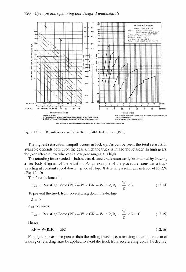
920 Open pit mine planning and design: Fundamentals
Figure 12.17. Retardation curve for the Terex 33-09 Hauler. Terex (1978).
The highest retardation rimpull occurs in lock up. As can be seen, the total retardationavailable depends both upon the gear which the truck is in and the retarder. In high gears,the gear effect is low whereas in low gear ranges it is high.The retarding force needed to balance truck acceleration can easily be obtained by drawing
a free-body diagram of the situation. As an example of the procedure, consider a trucktraveling at constant speed down a grade of slope X% having a rolling resistance of R0Ri%(Fig. 12.19).The force balance is
Fnet = Resisting Force (RF) + W × GR − W × RoRi = W
g× a (12.14)
To prevent the truck from accelerating down the decline
a = 0
Fnet becomes
Fnet = Resisting Force (RF) + W × GR − W × RoRi = W
g× a = 0 (12.15)
Hence,
RF = W(RoRi − GR) (12.16)
For a grade resistance greater than the rolling resistance, a resisting force in the form ofbraking or retarding must be applied to avoid the truck from accelerating down the decline.

Haulage trucks 921
Figure 12.18. Enlarged view of a torque converter – lock-up section of a retarder curve. Terex (1981).
Figure 12.19. Diagrammatic repre-sentation of a truck traveling down adecline.
Figure 12.20. Truck traveling alonga horizontal segment.
Assume that a fully loadedTerex 33-09 truck is truck traveling at 30mph along a horizontalsurface having a rolling resistance of 2% (see Fig. 12.20).If the truck is simply allowed to coast to a stop (no retardation or braking force is applied),
the truck would slow down due to the action of the rolling resistance alone. The stopping

922 Open pit mine planning and design: Fundamentals
distance can be found in the followingway. Using equation (12.13) one finds that the averagedeceleration is
−W × RoRi = W
g× a (12.17)
Or
a = −0.644 ft/sec2
The stopping distance (x) is found using the familiar equation
V2 = V2o + 2ax (12.18)
WhereV= final velocityVo = initial velocityx= distance traveleda= average acceleration
Substituting the appropriate values in equation (12.17) one finds that
x = 1503 ft
If, instead of being able to roll unhindered to a stop, a retardation force of 10,000 lbs. wascontinually applied, the deceleration would be
a = −2.23 ft/sec2
and the truck would stop in
x = 434 ft
For a truck rolling down a negative grade of 2%, at least in theory, the truck wouldmaintain a constant velocity even with the engine shut off. As the slope of the downwardgrade is increased, the truck would accelerate unless the retarder or the brakes were applied.Assume a vehicle weighing 203200 lbs enters a stretch of road for which the rolling
resistance is 2% and the grade is −8%. The total resistance is thus −6%. The retardingforce required to keep the vehicle from accelerating is
RF = −0.06 × 203200 = −12192 lbs.
If the vehicle enters the grade at a speed of 30mph, the available retardation as read fromFigure 12.17 is only about −10400 lbs. If nothing more were done, the vehicle would con-tinue to accelerate down the grade. However the service brakes can be applied to reduce thespeed to below22.5mphwhere the retarderwould once again control the speedof the vehicle.The values in Table 12.12 refer to the peak values for the different gear ranges.For a given gross vehicle weight and total resistance, retarder charts provide a wide range
of speeds over which the truck remains under retarder control (see Fig. 12.21).If one uses the maximum speed (point a) then an optimistic estimate of travel time would
be calculated. On the other hand use of the minimum value (point b) would yield a veryconservative estimate. The true value is probably somewhere in between. Some of the factorswhich affect this are
• road conditions• time of day

Haulage trucks 923
Table 12.12. Peak values as read from the retardation curve.
Velocity Retarder Force(mph) (lbs)
7.6 −4240011.4 −2850015.1 −2130022.5 −1430030.4 −1060045.4 −7100
Figure 12.21. Example application of the retarder curve. Terex (1981).
• experience of driver• level of traffic.Table 12.13 presents some maximum recommended values which can be used for
estimating.
12.4.5 Specifications for a modern mechanical drive truck
TheTerex 33-09 truck used to demonstrate the principles in the previous sectionwasmodernin the 1980’s. To illustrate the changes which have occurred over this period of time and toprovide the reader with a chance to practice the concepts learned, the specifications for amodern Terex truck, the Terex TR-100 shown in Figure 12.22, have been included in thissection (Terex, 2012).

924 Open pit mine planning and design: Fundamentals
Table 12.13. Maximum recommended downgrade speeds.
Recommend Downgrade SpeedsGrade (%) Speeds (mph)
0–6 30–357–8 21–259–10 17–2011–12 13–16Over 12 Less than 13mph
Figure 12.22. Photo of the Terex TR100 truck. Terex (2012b).
Figure 12.23 presents several drawings showing the truck geometry. Table 12.14 pro-vides the weights and payload dimensions. Figures 12.24 and 12.25 provide the respectiveperformance and retardation curves.At this point in time it is considered worthwhile to demonstrate the use of the performance
curve shown in Figure 12.24. Assume that the truck is loaded to its maximum payload of100 tons. In this case, the gross vehicle weight is 347715 lbs. The vertical line correspondingto this value is located toward the right side of Figure 12.24. Beginning at the top of thegraph, one follows the line vertically downward until the appropriate total resistance lineis intersected. Assuming that the rolling resistance is 2% and the grade resistance is 8%,the total resistance is 10%. From the intersection point, one moves horizontally until theperformance curve for the truck is intersected. In this case, one finds that the truck is in gear2. Moving vertically downward, it is found that a speed of about 8.8mph can be maintainedon this ramp segment. The interested reader is encouraged to repeat this procedure assumingthat the fully loaded truck is travelling down a grade of 8%. Assume a rolling resistance of2%. The retardation curve shown in Figure 12.25 is used.

Figure 12.23a. Dimensions of the Terex TR100 truck. Terex (2012b).
Figure 12.23b. Dimensions of the Terex TR100 truck. Terex (2012b).

926 Open pit mine planning and design: Fundamentals
Figure 12.23c. Dimensions of the Terex TR100 truck. Terex (2012b).
Table 12.14. Weight/payload of the Terex TR100 truck.Terex (2012b).
Net weight 159,895 lbs (72,530 kg)
Payload, maximum 187,810 lbs (85,190 kg)
Maximum Gross Weight∗ 347,715 lbs (157,720 kg)
∗Maximum permissible gross vehicle weight with options,attachments, full fuel tank and payload.
Weight Distribution Front Axle Rear Axle
Empty 49% 51%
Loaded 34% 66%
Maximum Gross Weight 347715 lbs (112690 kg)
Gross Engine Power 1050 hp (783 kW)
Maximum Payload 100 tons (91 metric tons)
Heaped Capacity 74.5 yd3 (57.0m3)

Haulage trucks 927
Figure 12.24. Performance curve for the Terex TR100 truck. Terex (2012b).
In this text, the term “performance curve” has been used to denote the curve being usedwhen the total resistance is positive. The term “retardation curve” has been applied tothe curve being used when the total resistance is negative. This simplifies the discussionand removes some potential confusion. Taken together the two curves describe the overall“performance” of the truck.
12.4.6 Braking systems
Brakes have been the standard way of slowing down and stopping vehicles over the years.They function by forcing a stationary surface against that rotating and a frictional force isdeveloped. Several different types of mechanical braking systems are used. Figure 12.26 isa diagrammatic view of a disk brake system.For all of the systems, the change in potential energy of the truck is translated into heat
energy. This heat must be carried away from the brake area otherwise damage can resultmaking the brakes ineffective. This is often the reason why trucks or even cars sometimesrunaway on long steep downhill grades.

928 Open pit mine planning and design: Fundamentals
Figure 12.25. Retardation curve for the Terex TR100 truck. Terex (2012b).
Figure 12.26a. Diagrammatic view of adisk braking system. Komatsu (2012)

Haulage trucks 929
12.5 PROPELLING THE CONTAINER – ELECTRICAL DRIVE SYSTEMS
12.5.1 Introduction
In the way of a brief review, three types of drive train are currently in use (Humphrey andWagner (2011)):
1. Mechanical drive2. Electrical drive
a. Direct-current (DC) electric driveb. Alternating-current (AC) electric drive
Themechanical drive train (which was the subject of the prior section) contains fivemajorcomponents (Humphrey and Wagner (2011):– engine– torque converter– transmission– differential– planetary gear sets (wheels)The power source is the diesel engine plus torque converter which transmits rotational
power from the engine to the main driveshaft. Machine torque and speed are controlled bythe transmission during operation. The differential transfers output torque to the wheels.Finally, the entire system is activated by means of a variety of electronic control modulesand hydraulic control systems.DC and AC electric drive trains contain six major components (Humphrey and Wagner
(2011):– engine– generator– power converter– wheel motors– planetary gear sets (wheels)– retarding gridThe power source is the diesel engine plus generator. The latter converts mechanical
power from the engine into electric power. AC current from the generator is then convertedinto useable form. In a DC-drive truck, a rectifier converts it into DC power. In anAC-drivetruck, a rectifier converts it into DC power and inverters convert it back to a controllableversion of AC power suitable for managing the amperes, volts and frequencies of the wheelmotors in order to create machine speed and torque. The DC orACwheel motors receive theelectric power and feed it mechanically to the planetary gear sets (wheels). The retardinggrid – a bank of resistor elements – provides braking force by turning the wheel motorsinto generators, creating power rather than receiving it. The power is sent through a controlcabinet and on to the resistor elements. The resistors impede the flow of the electric power,which causes the wheel motors to slow rotation. Heat generated is cooled by an electric fan(Humphrey and Wagner, 2011).In considering the advantages and disadvantages of the electrical and mechanical drive
systems one finds (Birkhimer, 2011) that electric-drive trucks, typically:• travel at higher speed on grades ranging from 4% to 10%• have potentially lower maintenance costs• offer slightly better fuel economy

930 Open pit mine planning and design: Fundamentals
Figure 12.26b. Cutaway showing the propulsion system. Komatsu (2012).
• have a smoother operator ride• offer better retarding capacity to stop the truck
On the other hand, they• have higher capital cost• require more specialized technical training and capabilities
In comparison, mechanical drive trucks:• more effectively travel on steeper grades (greater than 10%)• have a larger market presence resulting in more knowledge in the field• have a lower capital cost• require a lower level of technical specialization• are lighter weight vehiclesAs indicated, within the electric-drive option, there is a choice to be made between
direct current (DC) and alternating current (AC). The AC-drive offers advantages over theDC-drive and is becoming the more common choice in today’s market (Berkhimer, 2011).The remainder of this section will focus on the AC-drive option.
12.5.2 Application of the AC-drive option to a largemining truck
This section is based entirely on material kindly provided by Siemens (2012) and Komatsu(2012). Figure 12.26b presents a cutaway of a large haulage truck showing the componentsof the AC-drive propulsion system.Figures 12.27 and 12.28 present different schematic views of the wheel motor assembly.A block diagram depicting the elements in the AC-drive system is presented in
Figure 12.29.

Haulage trucks 931
Figure 12.27. Diagrammatic representation of a wheelmotor assembly. Komatsu (2012).
Figure 12.28. Diagrammatic representation of a wheel motor. Komatsu (2012).
Figure 12.29. Block diagram showing the components of a typical electric drive system. Siemens (2012a).

932 Open pit mine planning and design: Fundamentals
In general terms, during propulsion, the traction alternator converts themechanical energyof the diesel engine into DC current, charging the DC bus capacitors. The electric powerpasses through the capacitors to two inverters, which produce AC current for the tractionmotors (M). The output frequency and voltage of the inverters is controlled to provideprecise motor torque and speed. In the retardation mode, the motors apply braking forceby generating electricity which is converted to DC by the inverters. Braking choppers,connected to the inverters, channel that power straight into a resistor grid that continuouslydissipates the energy until the truck reaches standstill (the stop position). So braking issmooth, like driving a car, but without mechanical brake wear (Siemens, 2012a).Each of the components shown in Figure 12.29 will now be briefly described (Siemens,
2012a):1. The power unit consists of the diesel engine, the alternator, and the rectifier. AC power
generated in the alternator is converted to 1,500V DC in the rectifier and flows throughthe DC link capacitors to the traction inverters.
2. The inverters, motors, and alternator are cooled by a dedicated electric blower thatoperates independently of vehicle speed or engine rpm. This maximizes cooling per-formance and system reliability. The inverters, controlled by a specialized controlunit, transform DC power at constant voltage into AC power at variable frequencyand voltage to drive the truck wheel motors. During braking, the inverters send powerfrom the motors back to the DC link. The inverters allow high switching frequencies,which improves the current quality to the motors. This means the drives require nosnubbers (devices to suppress or “snub” voltage transients), and smaller, less complexgate drivers. They have a high overload capability, which enables electronic protectioncircuits without fuses. This results in greatly increased reliability.
3. Robust, high-torque, squirrel-cage induction motors with integrated speed sensorspower the two-stage planetary wheel gears.
4. Maintenance-free electric braking choppers are used in place of mechanical contactorsto connect the powerful grid resistors. The retard pedal initiates immediate and smoothbraking action. Capable of dissipating up to 6,000 horsepower, the braking systemimproves control and greatly reduces mechanical brake wear.
5. The auxiliary power system functions both as a rectifier and as a generator.6. The water cooling system is completely self-contained. The speed and cooling are
controlled by numerous sensors. The liquid pump circulates coolant to/from the radi-ator while the air heat exchanger equalizes the coolant temperature with the cabinettemperature. The high power density, closed-cycle cooling, and standardized modulesoptimize the system’s capability, reliability, and efficiency.
7. The drive system has a very high tractive effort (rimpull) for pulling away in softground and fully utilizes all available engine horsepower. Retard utilizes the full powercapability of the AC drive system for the highest safe downhill speeds.
12.5.3 Specifications of a large AC-drive mining truck
Figure 12.30 shows the Komatsu 860E electric drive truck. The truck is able to carry a280 ton payload and weighs 1,001,700 lbs when fully loaded. It is powered by a KomatsuSSDA16V160 engine which delivers 2700 hp. The AC drive is supplied by Siemens.The specifications for the truck are given in Tables 12.15–12.17 and in Figures
12.31–12.33.

Haulage trucks 933
Figure 12.30. Photo of the Komatsu 860E truck. Komatsu (2009a).
Table 12.15. The weight/payload of the Komatsu 860E truck. Komatsu (2009a).
Vehicle WeightsStandard Chassis 137325 kg 302,749 lbsKomatsu Body 33643 kg 74,171 lbsStandard Tile Weight 23033 kg 50,780 lbsOption Allowance 6350 kg 14,000 lbs
Empty Vehicle Weight 200351 kg 441,700 lbsFront Axle (49%) 98361 kg 216,850 lbsRear Axle (51%) 101990 kg 224,850 lbs
Max. Gross Vehicle Weight 454363 kg 1,001,700 lbsFront Axle (33.5%) 152392 kg 335,871 lbsRear Axle (66.5%) 301971 kg 665,829 lbs
Nominal Payload 254363 kg 560,000 lbs254 metric tons 280 short tons
Nominal payload is defined by Komatsu America Corp’s payload policydocumentation. In general, the nominal payload must be adjusted for the specificvehicle configuration and site application. The figures above are provided forbasic product description purposes. Please contact your Komatsu distributor forspecific application requirements.
12.5.4 Calculation of truck travel time
Figure 12.34 shows the path to be taken by the Komatsu 860E truck in going from the shovelto the dump and return.The characteristics of the segments are given in Table 12.18.

934 Open pit mine planning and design: Fundamentals
Table 12.16. Specification sheet (1) for the Komatsu 860E truck. Komatsu (2009a).
Make and model Komatsu SSDA16V160 Tier 2Fuel DieselNumber of cylinders 16Operating cycle 4 cycleGross horsepower∗ @ 1900 rpm 2,700HP 2014 kWNet flywheel power∗∗ @ 1900 rpm 2,550HP 1902 kWWeight (wet) 21,182 lb 9608 kg
∗Gross horsepower is the output of the engine as installed in this machine, at governed rpm and with enginemanufacturer’s approved fuel setting. Accessory losses included are water pump, fuel pump and oil pump.∗∗Net flywheel power is the rated power at the engine flywheel minus the average accessory losses.Accessories include fan and charging alternator. Rating(s) represent net engine performance in accordancewith SAE J1349 conditions.
Table 12.17. Specification sheet (2) for the Komatsu 860E truck. Komatsu (2009a).
DimensionsBox Dimensions 30 ft. 3 in.× 27 ft. 4 in. (9.21× 8.33m)Overall Length 49 ft. (14.93m)Overall Height 23 ft. 11 in. (7.3m)Overall Width 30 ft. 10 in. (9.39m)Wheelbase 20 ft. 8 in. (6.3m)Weight Empty: 4441,700 lbs. (200,351 kg)
Engine & DrivetrainEngine Make KomatsuEngine Model SSDA16V160Engine Type 4-cycleHorsepower 2,700 hp (2,014 kW) @ 1,900 rpmFuel Type DieselTank Capacity 1,200 gal. (4,542 l)
OperationalBrakes Service brakes, emergency brakes, wheel brake locks, parking brakes,
electric dynamic retarderSuspension Variable rate hydro-pneumatic with integral rebound control.Tires 50/80 R57Steering Accumlator-assisted twin cylinders provide constant rate steering.
DimensionsPayload 560,000 lbs. (254,363 kg)
OperationalNumber of Rear Axles 1
Assuming the truck is loaded to its rated capacity and using the Komatsu Travel TimeSimulator, it is found that (Komatsu, 2012a):
loaded haul = 12.4 minutes
empty return = 3 minutes
In running this example, no speed limits have been imposed. The interested reader isencouraged to try and duplicate these values using the two manual approaches described insection 12.7.

Haulage trucks 935
Figure 12.31. Dimensions of the Komatsu 860E truck. Komatsu (2009a).
Figure 12.32. Performance curve for the Komatsu 860E truck. Komatsu (2012).

936 Open pit mine planning and design: Fundamentals
Figure 12.33. Retardation curve for the Komatsu 860E truck. Komatsu (2012).
Figure 12.34. Haul profile used by the Komatsu 860E-K truck. Komatsu (2012a).

Haulage trucks 937
Table 12.18. Segment characteristics assumed. Komatsu (2012a).
Segment Length (ft) Grade Rolling Resistance
1 600 0% 2%2 400 4% 2%3∗ 6000 10% 2%4∗ 800 8% 2%5 600 0% 2%
12.6 PROPELLING THE CONTAINER – TROLLEYASSIST
12.6.1 Introduction
According to Humphrey and Wagner (2011),“A trolley-assist mining truck is a unique application for mining trucks and strictly exclu-
sive to electric-drive models. A trolley-assist mining truck draws its power from overheadpower lines that are run on haul segments where the largest benefits can accrue, such aswhere the loaded truck operates on a positive grade. The truck is fitted with a pantographthat acts as a conduit between the line and the truck’s electric-drive distribution system.As the truck approaches the line, the operator lifts the pantograph until it contacts theline. When the two engage, the operator removes his or her foot from the throttle andcontinues to steer while the truck draws power from the line. Power is fed to the wheelmotors, temporarily replacing the diesel engine and generator. Trolley assist has severalbenefits:
• Decreased fuel consumption, achieved by running the engine at idle for the length ofthe line. Depending on the length of the ramp, fuel savings can be as high as 50%.
• Increased productivity per cycle, achieved by using the excess power capacity of thewheel motors. The power rating of a wheel motor is almost twice the engine grosshorsepower, in order tomeet the technical requirements for continuous operation underdiesel power. That is the primary reason for the significant speed-on-grade performancein retarding, when the wheel motors use their full potential. The same principle appliesduring trolley assist, when power from the diesel engine is replaced by power from theoverhead line. The result is an increase of up to 80% in speed-on-grade performance.Depending on the haul cycle, this can translate into an increase in production of up to10%.
• Increased diesel engine lifetime. The heaviest toll on an engine in a haul cycle normallyoccurs when the truck is fully loaded on a grade – the very point at which trolley assistkicks in. The life of a diesel engine is calculated in terms of the total quantity of fuelconsumed during the design life. With the engine operating at idle on grade ratherthan at maximum, the life can be extended significantly, potentially eliminating onecomplete engine rebuild over the life of the truck.
Trolley assist also involves additional operational costs and constraints, including thefollowing:
• Relative costs of electric power and diesel. This is one of the single largest variables toconsider when evaluating trolley assist. The cost for diesel fuel can be enormous for
UFM
|484
942|
1435
6130
07

938 Open pit mine planning and design: Fundamentals
Figure 12.35. Trolley-equipped 860E truck. Komatsu (2008).
a medium to large fleet, but the ultimate question is whether the savings in fuel canoffset the cost of electric power.
• Capital cost of trolley wayside equipment. This consists of mine power distribution,substations, masts, and wire.
• Capital cost of truck trolley equipment. This consists of a pantograph, auxiliary cooling,and truck controls.
• Mine plan. Trolley assist does not allow for operational flexibility. After the equipmentis in place, it typically is not moved until doing so makes economic sense, often 5 to10 years from the initial installment. Therefore it is critical to evaluate the long-termmine plan and determine whether or not a permanent main haul road is possible.
• Haul profiles. Determining which haul cycle benefits from trolley assist is one of themost critical pieces to the evaluation. A long haul segment with a grade that the trucktravels loaded is the best choice.
• Capital cost for additional mine-support equipment. Costs associated with additionalmotor graders or wheel dozers may need to be included. Haul roads where trolleyassist is used must be kept in pristine condition, since spillage and rutting can causethe truck to lose connection with the overhead line.
The industry will continue to support trolley assist. Technology improvements nowunder consideration include concepts such as auto-control when ascending a grade andregeneration of power when retarding during a return cycle.”
12.6.2 Trolley-equipped Komatsu 860E truck
Figure 12.35 shows the trolley-equipped Komatsu 860E truck in the plant.
UFM
|484
942|
1435
6130
02

Haulage trucks 939
Figure 12.36. Truck operating under trolley power. Komatsu (2009a).
Figure 12.36 shows a trolley-equipped Komatsu 860E truck operating in an iron mine.In this case the trolley line is operated at 1800 volts DC.
12.6.3 Cycle time calculation for the Komatsu 860E truck with trolley assist
Figure 12.37 shows the performance curves for the Komatsu 860E truck with and withouttrolley assist.In reviewing the path shown in Figure 12.34 it will be assumed that a trolley line has
been constructed over segments 3 and 4. Assuming the truck has been loaded to its ratedcapacity, the haul time using the Komatsu Travel Time Simulator is now determined to be7.1 minutes compared to a time of 12.4 minutes without trolley assist (Komatsu, 2012a).The interested reader is encouraged to check this calculation using the methods describedin the following section.
12.7 CALCULATION OF TRUCK TRAVEL TIME – HAND METHODS
12.7.1 Introduction
Figure 12.38 shows a path to be taken by the Terex 33-09 truck in going from the shovel tothe dump and back. It is required to determine the time needed for the truck to complete thehaul and return portions.This section presents two hand methods by which this can be done.1. Equation of Motion Method2. Speed Factor Method

940 Open pit mine planning and design: Fundamentals
Figure 12.37. Performance curve for the Komatsu 860E truck with and without trolley assist. Komatsu(2012a).
Figure 12.38. Path taken by theTerex 33-09 truck.

Haulage trucks 941
12.7.2 Approach 1 – Equation of motion method
In this section, four examples will be presented to illustrate how the performance andretardation curves can be used to calculate
• the time required to traverse a given road segment• the exit speed• the average speed over a segmentIn the process of working the examples, the basic formulas will be introduced. With this
as background it is hoped that the reader can complete the calculations for the remainingroad segments. The examples will deal with the following segments:
Loaded Haul
Segment 1: Truck accelerating from rest
Segment 4: Entrance speed greater than that which can be maintained
Segment 6: Truck coming to a stop
Table 12.19. Summary of the coordinates for theperformance curve.
Velocity Rimpull(mph) (lbs)
Gear 1 0 640003.0 500004.5 400006.0 285006.01 315007.30 28000
Gear 2 7.31 250008.90 195008.91 2100010.6 19000
Gear 3 10.61 1750011.70 1450011.71 1600014.20 14000
Gear 4 14.21 1180017.50 1000017.51 1060021.30 9600
Gear 5 21.31 820023.70 700023.71 780028.50 7000
Gear 6 28.51 630035.40 490035.41 520042.50 480042.41 0

942 Open pit mine planning and design: Fundamentals
Empty Return
Segment 4: Downhill segment with a speed limit
The loaded and empty weights of the truck are 203,200 lbs and 93,200 lbs respectively.The first step in the process is to have digitized versions of the performance and retarda-tion curves. Table 12.19 gives the major coordinates of the performance curve shown inFigure 12.39.Table 12.20 provides similar values for the retardation curve (Fig. 12.40).
Figure 12.39. Performance curve for the Terex 33-09 truck with the coordinates given.

Haulage trucks 943
Figure 12.40. Retardation curve with the coordinates given.
Table 12.20. Retarder curve coordinates for the Terex 33-09 truck.
Velocity Rimpull Velocity Rimpull(mph) (lbs) (mph) (lbs)
2 5000 15.10 75005.50 25000 17.50 95005.50 32500 17.50 110007.60 42400 22.50 143007.60 15000 22.50 65008.75 18000 23.50 70008.75 23500 23.50 800011.40 28500 30.40 1060011.40 13000 30.40 400012.50 14500 35.40 470012.50 17000 35.40 550015.10 21300 45.40 7100

944 Open pit mine planning and design: Fundamentals
Loaded haul calculations
Segment 1. Truck Accelerating from RestThe length of this segment is 1000 ft, the grade resistance is 0%, the rolling resistance is3%, and the total resistance is 3%. The tractive effort required to overcome grade and rollingresistance (and to maintain a constant velocity) is
TEmin = 0.03(203200) ≥ 6100 lbs
For this example, it will be assumed that the coefficient of traction is 0.6. The weighton the rear (drive) tires is 135400 lbs. The maximum rimpull which can be exerted withoutspinning the wheels is
TE (max) = 0.6(135400) = 81240 lbs
As read from the Performance Curve, the maximum available rimpull is 64,000 lbs, hencethis is the controlling value. To simplify the discussion, the performance curve has beendivided into a series of regions each denoted by a Roman numeral which will be handled inthe forthcoming integration process.In Figure 12.41, the minimum rimpull line intersects the performance curve at a speed of
29.5mph. This is the maximum speed which can be achieved by the truck over this segment.The difference in force between that given by the performance curve and the minimum
(6100 lbs) is available to accelerate the truck. In this example, it will be assumed that theavailable force is fully utilized for acceleration.Over segment I, (From 0 to 3mph), the average rimpull is
RP (ave) = 64000 + 50000
2= 57000 lbs
The rimpull available for truck acceleration is
RP (acc) = 57000 − 6100 = 50900 lbs
Since the mass of the truck is
M (truck) = W
g= 203200 lbs
32.2 ft/sec2= 6311
lbs-sec2
ft
the average acceleration in this portion of the performance curve is
a = force
acceleration= 50900
6311= 8.07 ft/sec2
Knowing that the initial velocity (vi) is 0mph and the final velocity (vf ) is 3mph the timecan be calculated using
t = vf − via
(12.19)
Thus,
t = (3 − 0)
8.07
(5280
3600
)= 0.545 seconds

Haulage trucks 945
Figure 12.41. The regions involved in accelerating from rest (Segment 1).
The distance which would be traveled in this time can be calculated using either of thefollowing formulas
x = v2f − v2i2a
(12.20)
x =(vf + vi
2
)t (12.21)

946 Open pit mine planning and design: Fundamentals
Table 12.21. Summary of the hand calculated results for segment 1 based on using the equations of motion
Region V0 (MPH) V1 (MPH) RPnet (lbs) acc (ft/sec2) time (sec) distance (ft)
I 0 3 50900 8.07 0.55 1.20II 3 4.5 38900 6.16 0.36 1.96III 4.5 6 28150 4.46 0.49 3.80IV 6.01 7.3 23650 3.75 0.50 4.93V 7.31 8.9 16150 2.56 0.91 10.83VI 8.91 10.6 13900 2.20 1.13 16.10VII 10.61 11.7 9900 1.57 1.02 16.67VIII 11.71 14.2 8900 1.41 2.59 49.20IX 14.21 17.5 4800 0.76 6.34 147.53X 17.51 21.3 4000 0.63 8.77 249.61XI 21.31 23.7 1500 0.24 14.75 486.80XII 23.71 28.5 1300 0.21 34.11 1305.80
Substituting the appropriate values, one finds that
x = v2f − v2i2a
= (32 − 02)
2(8.07)
(5280
3600
)2
= 1.20 feet
x =(vf + vi
2
)t =
(3 + 0
2
)(5280
3600
)0.545 = 1.20 feet
This process is continued until either the maximum velocity of 29.5mph or the segmentlength of 1000 ft is reached. Table 12.21 summarizes the results.At the end of Region XI, the truck has traveled 988.6 ft and hence the travel distance of
1000 ft falls in Region XII. The final velocity would be
v2f = v2i + 2ax = 23.72 + 2(0.21)(11.4)
(3600
5280
)2
vf = 23.75mph
The time required to accelerate from 23.71mph to 23.75mph is 0.28 seconds and thetotal time required for the segment would be 37.59 sec. The average velocity would be
v = 1000 ft × 60 sec/min
37.59 sec= 1596 ft/min
or
v = 18.2mph
Segment 4. Entrance speed greater than that which can be maintained
This example will cover the situation when the truck has an exit speed of 23.83mph fromsegment 3 and encounters segment 4 which is 500 ft in length and the total resistance is 11%.For this segment, the minimum rimpull requirement is 22352 lbs and the velocity which canbe maintained is 8.2mph as read from the performance curve (see Fig. 12.42).The truck has an entrance speedmuch higher than can be sustained on such a segment. The
momentum of the truck however allows it to travel a considerable distance up the segmentbefore the steady state speed is reached. In this example, the exit speed, time to traverse

Haulage trucks 947
Figure 12.42. The regions involved in Segment 4.
the segment, average speed and the speed factor will be calculated. As can be seen fromFigure 12.42, there are eight segments which must be evaluated. Over segment II (from 23.7to 21.3mph) the average rimpull force is
RP (ave) =(8.2 + 7.0
2t
)103 = 7600 lbs
The difference between 7600 lbs and 22352 lbs is the deceleration force on the truck
RP (deceleration) = 7600 − 22352 = −14752 lbs

948 Open pit mine planning and design: Fundamentals
Table 12.22. Results for Segment 4 using the equations of motion.
Region Speed Range Ave Decel Time To Complete Dist. Total(mph) ft/sec2 (sec) Dist.
I 23.83→ 23.7 −2.31 0.76 2.9 3II 23.7→ 21.3 −2.34 1.51 49.6 53III 21.3→ 17.5 −1.94 2.88 82.1 135IV 17.5→ 14.2 −1.77 2.74 63.8 199V 14.2→ 11.7 −1.16 3.17 60.4 259VI 11.7→ 10.6 −1.01 1.61 26.4 285VII 10.6→ 8.9 −0.37 6.70 96.0 381VIII 8.9→ 8.2 −0.23 4.55 57.0 438
The deceleration is
a = −14752
6311= −2.34 ft/sec2
and the time required to go from 23.7mph to 21.3mph is
t =(21.3 − 23.7
−2.34
)5280
3600= 1.51 sec
The distance traveled in that time is
x =(21.3 + 23.7
2
)(5280
3600
)(1.51) = 49.8 ft
The process is repeated for the other regions in the same way. The results are given inTable 12.22.Thus only a stretch of 62 ft would be required to be traveled at 8.2mph which is the exit
speed. The time required for this short stretch would be 5.16 seconds and the total time forthe segment would be 29.08 seconds. The average speed becomes
vave = 500(60)
29.08= 1032 ft/min
vave = 11.72mph
Segment 6. Truck Coming to a Stop
The exit speed from segment 5 is 13.9mph and as can be read from the performance curve,the rimpull is 14224 lbs. Segment 6 has a length of 1000 ft, a grade resistance of 0% and arolling resistance of 6%.At the end of segment 6 the truck is stopped. For 6% total resistance,the required tractive effort is
TE (req) = 0.06 × 203,200 = 12,192 lbs
and the maximum velocity (in gear 3) is 14.2mph.Therefore the truck can increase its speed from 13.9mph to 14.2mph before beginning
to stop. Using the equations as before one finds that
F = (14224− 12192) = 2032 lbsa = 0.322 ft/sect = 1.37 secx = 28 ft

Haulage trucks 949
Thus in segment 6, there remains 972 ft for travel at 14.2mph and stopping. The questionto be answered is the stopping distance and time required. Three ways:
Case 1: Truck slowing due to rolling resistance onlyCase 2: The truck slowed using the retarder and stopped using the service brakesCase 3: The truck is slowed by following the full retarder curve.
will be examined.
Case 1: Truck slowing due to the rolling resistance only. If the truck is simply allowed toslow down because of the 6% rolling resistance, then
F (decel) = −12192 lbs
a = −1.93 ft/sec2
t =(0 − 14.2
−1.93
)1.47 = 10.82 sec
x = 112 ft
Case 2: The truck is slowed using the retarder and stopped with the service brakes.In this case it will be assumed that the retarder force is maintained such that an aver-
age deceleration rate of 15000 ft/min/min (4.17 ft/sec2) is maintained. Since the rollingresistance provides a deceleration rate of 1.93 ft/sec2 by itself, the retarder is requiredto contribute 2.24 ft/sec2. A minimum retarder force of 14136 lbs would be required.As seen from the retarder curve (Fig. 12.39), the minimum peak value is 21300 lbs. Itcould be maintained, except for the speed range of 8.75 to 7.5mph where it drops to13000 lbs at a speed of 3.5mph. At this point (or some point earlier) the service brakeswould be applied. If the deceleration rate of 4.17 ft/sec2 is applied from 14.2 to 0mphthen
t = 5.0 sec
x = 52 ft
Case 3: The truck is slowed by following the full retarder curve.In this case, the retarder curve is followed in the same way as was done with the perfor-
mance curve. The curve represents the maximum retarding situation with the retarder fullof oil. The initial speed of 14.2mph falls within sector I shown on Figure 12.43.The peak force is 19811 lbs. The average force due to the retarder in going from 14.2
to 12.5mph is 18406 lbs. This must be added to the retardation due to rolling resistance(12192 lbs) to yield a total retardation force of 30598 lbs. The deceleration, time and distancebecome
a (decl) = −4.85 ft/sec2
t =(12.5 − 14.2
−4.85
)1.47 = 0.52 sec
x =(12.52 − 14.22
−2(4.85)
)2.15 = 10.06 ft
The process described above is repeated for each of the other sectors. The results are givenin Table 12.23.For Region VII, the same deceleration as Region VI was used.

950 Open pit mine planning and design: Fundamentals
Figure 12.43. Application of the retardation curve.
Table 12.23. Results for Segment 6, truck coming to a stop, using the equations ofmotion approach.
Region Velocity Range Total Retarding Deceleration Time Distance(mph) Force (lbs) (ft/sec2) (sec) (ft)
I 14.2→ 12.5 30598 −4.85 0.52 10.06II 12.5→ 11.4 25942 −4.11 0.39 6.88III 11.4→ 8.75 38192 −6.05 0.64 9.49IV 8.75→ 7.6 32756 −5.19 0.33 3.89V 7.6→ 5.5 49642 −7.87 0.39 3.78VI 5.5→ 2 27192 −4.31 1.19 6.55VII 2→ 0 27192 −4.31 0.68 1.00
The total distance traveled is 41.65 ft and the time required is 4.14 sec. In this partic-ular case the rate of deceleration varies from 4.11 ft/sec2 up to 7.87 ft/sec2. In practice,the operator would try to maintain a smooth retardation action. This is discussed in thefollowing case.

Haulage trucks 951
Table 12.24. Summary of the hand-calculated results based on using the equations of motion.
Segment Length Imposed Entrance Exit Average Time Accum.Number (ft) Speed Limit Speed Speed Speed (sec) Time
(mph) (mph) (mph) (mph) (min)
Haul1 1000 – 0 23.75 18.2 37.45 0.622 1500 – 23.75 30.00 29.7 34.40 1.203 750 30 30.00 23.83 26.6 19.17 1.524 500 – 23.83 8.2 11.7 29.08 2.005 1000 – 8.2 13.9 12.8 53.26 2.896 1000 – 13.9 0 13.5 50.54 3.73Return6 1000 – 0 28.9 22.0 31.04 0.525 1000 – 28.9 22 34.3 19.90 0.854 500 22 22 22 22 15.50 1.113 750 – 22 30.44 27.2 18.80 1.422 1500 – 30.44 26.9 28.5 35.84 2.021 1000 – 26.9 0 25.3 26.90 2.47
The third approach will be adopted here and a deceleration rate of 4.17 ft/sec2 will beapplied to all of the retarder situations in this book.Since the acceleration from 13.9 to 14.2mph requires 1.37 sec and consumes 28 ft and
the deceleration from 14.2mph to 0 requires 5 sec and 52 ft, the middle stretch of 920 ftwill be traveled at 14.2mph. This requires 44.17 seconds. The total time for the segment is50.54 seconds and the average speed is 13.5mph.
Empty return calculations
Segment 4: Downhill segment with speed limitOn this downhill empty return segment, the speed limit is 22mph. The total resistance is−5% and the length is 500 ft. The rimpull required to keep the truck from accelerating is
RP = 0.05(93200) = 4660 lbs
Using a segment entrance speed of 22mph, the retardation rimpull available is 14500 lbs(4th gear). Therefore, no difficulty would be expected to maintain the 22mph. The time forthis segment would be 15.50 seconds.Table 12.24 presents the results for all of the segments done by hand.
12.7.3 Approach 2 – Speed factor method
In the previous section, a hand procedure to calculate truck velocities and travel timesusing well known force/acceleration/velocity/distance equations and truck performance/retardation curves was described. The results of applying this process for the Terex 33-09truck for the path shown in Figure 12.38 have been given in Table 12.24. The process is verytime consuming and cumbersome. If the route or truck is changed, the entire process wouldhave to be repeated. One alternative to this is the computerization of the equations. Several

952 Open pit mine planning and design: Fundamentals
Table 12.25. Maximum speeds as read from theperformance (P) and retardation curves (R).
Segment Speeds Read FromPerformance (P)/Retardation (R)Curves (mph)
Haul1 29 (P)2 42.4 (R)3 20 (P)4 8.4 (P)5 14.0 (P)6 14.4 (P)Return6 32.5 (P)5 42.4 (P)4 30.5 (R)3 42.4 (P)2 27.0 (P)1 42.4 (P)
Table 12.26. Average speed as determined from thehand calculations.
Segment Average Speed (mph)
Haul1 18.22 29.73 26.64 11.75 12.86 13.5Return6 22.05 34.34 22.03 27.22 28.51 25.3
such programs are commercially available. Various truck manufacturers also provide cyclecalculations as a service to their customers. There is, however, another hand procedurewhich can be followed yielding useable results rather quickly. This procedure based uponthe use of speed factors is described in this section. The theory will be illustrated throughdiscussion of the Terex 33-09 truck example.Knowing the total resistance and the vehicle weight, the maximum speeds which the
truck is capable of achieving over a given segment can be read directly from the appropriateperformance/retardation curve. Such values for the example are given in Table 12.25.The average speed values over these same segments as determined using the equation of
motion approach are given in Table 12.26.

Haulage trucks 953
Table 12.27. Calculated speed factors.
Segment Calculated Segment CalculatedHaul Speed Factor Return Speed Factor
1 0.61 6 0.692 0.98 5 0.813 1.33 4 1.004 1.44 3 0.655 0.92 2 1.056 0.94 1 0.60
The ratio of the average speed (Table 12.26) to the performance/retardation values(Table 12.25) can be easily found.
SF = average segment speed/curve (mph)
performance/retardation speed (mph)(12.22)
This ratio (called the speed factor (SF)) is given in Table 12.27.To obtain the desired segment time, the average speed values (Table 12.26) are applied
to the corresponding segment lengths. If, instead of calculating speed factors as a last stepin the process, one could read the values from a table, then the step of determining averagevelocity could be greatly simplified. It would become
average velocity = SF (Table) × Performance/Retardation Curve Value (12.23)
Clearly the key to this process is having a general table of speed factors from which onecould select the needed values for any combination of the following operating conditions:
• empty and loaded truck situations• starting from rest• coming to a stop• various segment lengths• level, uphill and downhill segments entered while in motion.Table 12.28 presents speed factors which can be used for this purpose.Some explanation dealing with this table will now be presented.Various truck loading conditions (empty, loaded, partially loaded) are handled through
the use of a weight to power ratio (WPR).
WPR = Vehicle weight (lbs)
Flywheel (brake) horsepower(12.24)
Through this calculation, one determines which of the three sections of the table shouldbe used. For loaded and empty hauls one would generally be in different sections of thetable.For the fully loaded Terex Truck
Weight = 203200 lbs
HP = 624
and therefore
WPR = 203200
624= 326 lbs/hp

954 Open pit mine planning and design: Fundamentals
Table 12.28. Published speed factors. Terex (1984).
under 300 lbs/hpMaul Road Level Haul Unit in Motion When Entering Haul Road SectionLength in Unit StartingFeet from 0MPH Level Downhill Grade Uphill Grade Factor
0–200 0–.40 0–.65 0–.67 1.00201–400 .40–.51 .65–.70 .67.–72 (Entrance speed greater than401–600 .51–.56 .70–.75 .72–.77 maximum attainable speed601–1000 .56–.67 .75–.81 .77–.83 on section)1001–1500 .67–.75 .81–.88 .83–.901501–2000 .75–.80 .88–.91 .90–.932001–2500 .80–.84 .91–.93 .93.–952501–3500 .84–.87 .93–.95 .95.–973501 & up .87–.94 .95– .97–
300—380 lbs/hp0–200 0–.39 0–.62 0–.64 1.00201–400 .39–.48 .62–.67 .64–.68 (Entrance speed greater401–600 .48–.54 .67–.70 .68–.74 than maximum attainable601–1000 .54–.61 .70–.75 .74–.83 speed on section)1001–1500 .61–.68 .75–.79 .83–.881501–2000 .68–.74 .79–.84 .88–.912001–2500 .74–.78 .84–.87 .91–.932501–3500 .78–.84 .87–.90 .93–.953501 & up .84–.92 .90–.93 .95–.97
380 & up lbs/hp0–200 0–.33 0–.55 0–.56 1.00200–400 .33–.41 .55–.58 .56–.64 (Entrance speed401–600 .41–.46 .58–.65 .64–.70 greater than maximum601–1000 .46–.53 .65–.75 .70–.78 attainable speed on section)1001–1500 .53–.59 .75–.77 .78–.841501–20OO .59–.62 .77–.83 .84–.882001–2500 .62–.65 .83–.86 .88–.902501–3500 .65–.70 .86–.90 .90–.923501 & up .70–.75 .90–.93 .92–.95
For the empty Terex Truck
WPR = 93200
624= 149 lbs/hp
The table distinguishes between vehicles which are starting from rest and those alreadyin motion when entering the segment.For a vehicle accelerating from rest along a level (grade resistance= 0) surface, the first
column in the table is used. Assuming WPR= 326, the speed factor for a segment lengthof 200 ft is 0.39. If the length had been 800 ft instead, interpolation yields a speed factor of0.575. There is often confusion regarding the correct column to be used when the unit is inmotion. The authors have found the following procedure to eliminate much of the difficulty.The total resistance values are examined for each segment. This is illustrated in Table 12.29.

Haulage trucks 955
Table 12.29. Resistance values and speed factors for selected segments.
Resistance
Segment Grade Rolling Total Speed Factor Column
1 0 2 2 Level2 8 2 10 Uphill3 5 2 7 Downhill
If the grade resistance for the current segment is zero, then the level column is used.When the grade resistance is not zero, then the total resistance (TR) of the previous segmentand the current segment are compared. In determining the proper speed factor column forsegment 2, one can see that
TR(2) > TR(1)
and thus the uphill factor applies.Since the grade resistance of segment 3 is 5%, the truck would continue to gain elevation
with distance. Technically it would be labeled as an uphill haul segment. However
TR(3) < TR(2)
and thus the truck would react as if it were going downhill as compared to the previoussegment.The effective grade change (EGC) defined as
EGC = TR(i) − TR(i − 1) (12.25)
should be used in deciding which column is appropriate. In this case
EGC = −3%
which is downhill compared to the previous segment. Hence the downhill column would beused.In general, as the length of the segment is increased, the vehicle will spend more time at
its maximum speed. This means that for vehicles starting from rest, moving on the level,or traveling on downhill grades, the speed factor tends toward 1.0 with increasing segmentlength. However for trucks encountering an uphill segment, the speed factor may increaseor decrease with segment length. If the vehicle speed on entering the segment is greater thanthat which can be maintained, then the speed factor decreases to 1.0 with distance. If theentrance speed is less than that which can be maintained on the grade, then the speed factorgradually increases to 1.0. As can be seen, a constant value of 1.0 is used in the chart.This illustrates an important limitation to the speed factor chart which is that conditions
existing in preceding or following segments are not considered. The “momentum effects”are important when entrance speeds are greater than those which can be maintained over along segment and the segments are short in length.For a vehicle in motion coming to a stop, the first column is used once again. However
in this case the lowestWPR section (under 300 lbs/hp) should be applied irrespective of thetrue WPR value. This means that for a vehicle having WPR= 326 stopping at the end of a200 ft long level segment, a speed factor of 0.40 should be used.

956 Open pit mine planning and design: Fundamentals
Table 12.30. Results of applying the speed factor approach by hand.
Segment Segment Speed Performance/ Speed Average SegmentLength Limit Retardation Factor Speed Time(ft) (mph) Curve Speed Used (mph) (min)
(mph)
Haul1 1000 – 29.0 0.61 17.7 0.642 1500 30 30.0 (42.4) 1.0 (0.88) 30.0 0.573 750 – 19.0 0.72 13.7 0.624 500 – 8.4 1.0 8.4 0.685 1000 – 14.0 0.83 11.6 0.986 1000 – 14.4 0.67 9.6 1.18
4.67Return6 1000 – 32.5 0.67 21.8 0.525 1000 – 42.4 0.83 35.2 0.324 500 22 22.0 (30.5) 1.0 (0.745) 22.0 0.263 750 – 42.4 0.77 32.6 0.262 1500 – 27.0 1.0 27.0 0.631 1000 ∼ 42.4 0.67 28.4 0.40
2.39
Haul time = 4.67minReturn time = 2.39minTotal time = 7.06min
A complication in this approach is the treatment of speed limits. If the maximum speedwhich can be achieved over the segment is less than the speed limit, the normal process isapplied. If, however, it is greater than the speed limit, a constant velocity equal to the speedlimit is used and the speed factor is 1. For the segment preceding the speed limit section, nospeed correction (reduction) is made. The results of applying the speed factor approach tothe Terex example are given in Table 12.30.
12.8 CALCULATION OF TRUCK TRAVEL TIME – COMPUTER METHODS
Over the years, different computer programs to calculate truck travel times have beendeveloped. In this section, two different approaches will be described:1. Based on the equation of motion2. Based on the speed factor approachThe results of applying both methods to the Terex 33-09 example discussed earlier will
be presented here.
12.8.1 Caterpillar haulage simulator
The results of applying the Caterpillar Fleet Production and Cost Simulator are given inTable 12.31.As can be seen, the results are similar to those given in Table 12.30 and particularly to
those given in 12.24.

Haulage trucks 957
Table 12.31. Computer generated output for the Terex 33-09 example.
Course–HAUL SEGMENTInitial Vehicle Speed = 0.00Haul RoadSeg Dist Roll Grade Vel Max SS Top Last Ac cumNo. (ft) Res Res. Limit Vel Vel Vel Time
(%) (%) (mph) (mph) (mph) (mph) (mph)
1 1000 3.0 0.00 0.00 29.01 23.97 23.97 0.622 1500 3.0 −5.00 30.00 42.41 30.00 30.00 1.203 750 5.0 0.00 0.00 19.47 30.00 23.53 1.524 500 3.0 8.00 0.00 8.37 23.53 8.94 1.975 1000 4.0 3.00 0.00 14.20 14.20 14.20 2.826 1000 6.0 0.00 0.00 14.21 14.21 0.00 3.65
Course–RETURN SEGMENTInitial Vehicle Speed= 0.00Return Road
Seg Dist Roll Grade Vel MaxSS Top Last AccumNo. (ft) Res Res Limit Vel Vel Vel Time
(%) (%) (mph) (mph) (mph) (mph) (mph)
6 1000 6.0 0.00 0.00 30.55 28.55 28.55 0.525 1000 4.0 −3.00 0.00 42.41 41.47 22.0 0.854 500 3.0 −8.00 22.00 42.41 22.00 22.00 1.113 750 5.0 0.00 0.00 37.95 30.45 30.45 1.432 1500 3.0 5.00 0.00 25.97 30.45 26.69 2.041 1000 3.0 0.00 0.00 42.40 36.26 0.00 2.46
Haul time= 3.65minReturn time= 2.46min
12.8.2 Speed-factor based simulator
Loy (1985c) has presented a computer program to calculate truck travel times based uponthe use of speed factors. Equations relating speed factor to distance have been developed foreach of the weight/horsepower groups and operating conditions given in the speed factorchart. They have the form
SF = adb (12.26)
wherea,b= constantsSF= speed factord= distance (ft).Table 12.32 presents the values of a and b which have been used in the program.The results for the Terex 33-09 truck are given in Table 12.33.Some differences are observed in the results between Tables 12.30 and 12.33. These are
due primarily to momentum effects and the way that speed limits are handled. Adjustmentscan be made in the starting and end points of the segments to at least partially eliminate thiseffect.

958 Open pit mine planning and design: Fundamentals
Table 12.32. Values used by Loy (1985c) in his speed factor-based computer program.
Condition WPR< 300 lbs/HP 300≤WPR < 380 WPR> 380
a b a b a b
Start from Stop 0.089 0.292 0.094 0.272 0.082 0.268Level Segment 0.298 0.146 0.304 0.133 0.193 0.193Downhill Segment 0.309 0.144 0.287 0.153 0.230 0.177Uphill Segment 1.0 0.0 1.0 0.0 1.0 0.0
12.9 AUTONOMOUS HAULAGE
The concept of “autonomous” haulage – the use of “driverless” trucks – is not new.According to Shelton (2010)
“In 1970, Unit Rig started designing a system that would allow a haulage truck,working in an open-pit mine, to operate driverless. Unit Rig teamed up with aSwedish firm, Saab-Scania, to develop and test a driverless truck. The driverless,“The Hands-Off Truck”, was shown at the AMC mining show in Las Vegas in1974. In 1976 Unit Rig operated a fleet of five M-100’s, utilizing the driverlesssystem, at Kennecott’s Chino Mine near Silver City, New Mexico. An interest-ing side note was that in order to get the labor union at the Chino mine to agreeto the driverless test, Unit Rig had to agree not to sell the system to this mine forten years. The test was successful and lasted several months and then was dis-assembled. The system did work but just was not practical with the technologyavailable at that time.”
The expression “Hands-Off Truck” was somewhat of an exaggeration. Truck guidance wasbased on the truck (without driver) following a cable buried in the haul road ramp. However,at the lower end of the cable line, control of the truck was taken over by an operator whomoved the truck to the shovel and after loading drove the truck back to the cable line. Atthe upper end of the line, an operator drove the truck to the dumping point, dumped andreturned the truck to the top of the line. It was an important first step.Zoschke (2001) has summarized some of the important milestones along the way toward
automation:• Early 1970’s Cable – laid systems in haul road• Early 1980’s Radio Transmitters• 1980’s Ground beacons, optical fiber gyros• Early 1990’s GPS operational system (prototype)• Mid 1990’s Refined GPS development• 1997 Integration of a supervisory system• 1998 Full cycle demonstration using AT supervisory systems• 1999, 2000 Integrated development and operational testing of a “production
capable” system• 2001 Real autonomous productionAccording to the Meeting Minutes from the Annual Meeting of the Western Mining
Electrical Association (Anonymous, 2001).

Haulage trucks 959
Table 12.33. Computer output using the speed factor approach.
SIMULATION PATH = LOADED HAUL FROM SHOVEL TO DUMPTRUCK UEIGHT= 203200 LBS.SEGMENT DISTANCE GRADE ROLLING TOTAL RES
(FT) (%) (%) (%)
1 1000 0 3 32 1000 −5 3 −23 750 0 5 54 500 8 3 115 1000 3 4 76 1000 0 6 6
SEGMENT SPD-LIMIT SPEED S-FACTOR SEG-TIME TOT. TIME(MPH) (MPH) (MIN) (MIN)
1 45 30 .615 .615 .6152 30 30 .878 .647 1.2623 45 19 .733 .611 1.8724 45 8 1 .71 2.5825 45 13 .825 1.059 3.6416 45 14 .668 1.215 4.656
SIMULATION PATH = RETURN EMPTY FROM DUMP TO SHOVELTRUCKWEIGHT= 93200 LBS.
SEGMENT DISTANCE GRADE ROLLING TOTAL RES(FT) (%) (%) (%)
1 1000 0 6 62 1000 −3 4 13 500 −6 3 −54 750 0 5 55 1500 5 3 86 1000 0 3 3
SEGMENT SPD-LIMIT SPEED S-FACTOR SEG-TIME TOT. TIME(MPH) (MPH) (MIN) (MIN)
1 45 33 .668 .515 .5152 45 44 .838 .306 .6223 22 22 .758 .34 1.1624 45 33 .783 .329 1.495 45 27 1 .631 2.1216 45 43 .668 .395 2.516
“Modular Mining working with Komatsu has developed a very repeatable andreliable system of operating a haul truck fleet sans the operator. Les Zoschkewalked us through a pictorial as well as technical overview of the 4 truck fleetthey have operating at a mine in Australia. The trucks are provided with GPSas well as inertial guidance systems operating in tandem, providing a guidancesystem that is so repeatable the trucks always follow the exact same tire track,braking and accelerating at the exact same point. Whole truck monitoring isprovided as is radar and other sensory systems which protect workers and other

960 Open pit mine planning and design: Fundamentals
equipment which ventures onto the haul road. Modular is so satisfied with thecurrent state of their technology that “babysitter operators” are no longer usedon the trucks. Les demonstrated the haul dump characteristics and single backuploading capability. He stated that double backup loading and highwall dumpingis something yet in the future. This is a technology still in the making.”
Nagai (2010b) of Komatsu stated
“In 2002, we got the official ‘go’ in the company for our development plan forAHS (Automated Haulage System), and kicked off the development ofAHS foruse in largemines.After developing and testing the system for about three years,in December 2005, we began testing a fleet of five 930E-AT driverless dumptrucks at CODELCO’s Radomiro Tomic mine. In January 2008, we formallydelivered 11 driverless dump trucks to CODELCO’s Gaby (Gabriela Mistral)coppermine, marking theworld’s first commercializationofAHS.OnDecember9, 2008, they held the opening ceremony to which Dr. Michelle Bachelet, thenPresident of Chile, was invited. Under stable operation, 11 units transported48.5 million tonnes (53.5 million U.S. tons) of material [24.5 million tonnes(27 million U.S. tons) of ore], and contributed to the production of 148,000tonnes (163,140 U.S. tons) of copper for the fiscal year ended March 31, 2009.When I heard this news, I felt all our hard work had totally paid off. Note: Asof June 30, 2010, 12 driverless dump trucks were working there”.
The early results from the fleet of driverless trucks at the Radomiro Tomic mine arepresented below (Meech, 2012):
• Tonnage hauled 2006= 8,222,000 t (32,000 tpd for 256 days)• Mechanical availability= 90.5%AHS vs 80.2% for total fleet• Effective utilization= 84.2%• Daily haulage time= 24× 0.0905× 0.842= 18.2 hrs
– percentage gain= 25.4%– potential to 20.5 hrs
• Accidents= none (2 in 2007)• Cost per tonne=U.S. $ 1.36/t which is much greater than the US $0.58/t normal• Maintenance reduction= 7%• Depreciation decrease= 3%• Impact on mine design:– Increased slope angle– Decreased road width
• Significant increase in safetyBriefly, the AHS functions in the following way (Anonymous, 2010a):• AHS is an integrated system to operate super-large driverless dump trucksautonomously by taking advantage of information and communication technologies(ICT) such as the high-precision global positioning system (GPS), obstacle detectionsensors, a wireless communication network system and a fleet management system.
• The fleetmanagement system operates driverless dump trucks. Information concerningtheir hauling routes and speed is sent wirelessly from the fleet management systemto the driverless trucks while they travel as they ascertain their position by using GPSinformation.

Haulage trucks 961
Figure 12.44. Sub-systems of an autonomous haulage truck (AHT). Parreira and Meech (2010).
• For loading, the fleet management system guides the trucks to the loading site, basedon the position of the bucket of the GPS-fitted, man-operated hydraulic excavator orwheel loader. After loading, the fleet management system directs the trucks with orealong the route to the dump site for unloading.
• ViaGPS and the wireless network, the fleet management system controls all equipmentin the mines, including other equipment and vehicles that are man-operated, to preventcollisions of driverless dump trucks. If the built-in obstacle detection sensors detectanother vehicle or person inside the haulage area during autonomous operation, thetrucks will stop immediately.
Figure 12.44 shows the various sub-systems of an autonomous truck considered in thesimulations performed by Parreira et al. (2010).The results from theAHT simulations and those obtained from simulations of a manually
operated truck system (truck drivers working 12-hour shifts on a 2-week-on/2-week-offschedule with all trucks running 24/7) were compared and expressed in the form of KeyPerformance Indicators (KPI). The results are shown below:
• Investment cost per truck +30%• Truck haulage cycle times −7%• Fuel consumption −10%• Tire wear −12%• Mechanical Availability +8%• Increased productivity +5%• Maintenance costs −14%• Increased truck life +12%• Labour costs −5%• Improved Safety/Reliability to be determined

962 Open pit mine planning and design: Fundamentals
The authors note that
“The expected improvement in labor costs is not particularly high. Despite therebeing no further need for four truck drivers (two on each cross shift cycle) foreach truck, additional personnel will be needed to maintain the trucks and theirsensor and control sub-systems. These employees will be much more skilledintellectually and thus, will have increased salaries.”
Rio Tinto (2012) has recently inaugurated a substantial and vital initiative, “The Mine ofthe Future (MOF)”, to help them find new ways to:1. Explore better2. Maximize their resources3. Go underground – deeper, faster and better4. Recover more from increasingly difficult deposits5. Do all the above safelyOverall, it is aimed at finding advanced ways to extract minerals deep within the Earth
while reducing environmental impacts and further improving safety. One of the key themesis to achieve a massive efficiency in surface bulk mining through autonomy. One importantpart of the move to greater autonomy is the introduction of a fleet of new driverless trucks,trains, drills and remote controlled equipment. By this means, productivity and safety areto be improved while enabling the employees to work from a site which is distant fromthe mine site. It should be noted that the program is not aimed at a single mine site butrather, once the technology has been proven, to be introduced across Rio Tinto. The ini-tial automation program has been established in Rio Tinto’s Iron Ore business in WesternAustralia. Working from their state-of-the-art Operations Center (OC) in Perth, employ-ees will eventually supervise automated drills, loaders and haul trucks across the Pilbarasites.Grad (2010) has provided the following description of some elements of the program:1. The West Angelas mine has become a de facto trial site for innovation such as
autonomous truck operation, automated drilling, and automated logistics applications.Pit A at the West Angelas mine has been designated as a pioneer site for MOF trials.
2. Under an alliance with Komatsu, Rio Tinto has been testing Komatsu’s FrontRunnerAutonomous Haulage System (AHS) with driverless trucks. There are presently fiveKomatsu 930E autonomous dump trucks (see Fig. 12.45) in operation there. Each haultruck, capable of carrying a 290-mt payload, is equipped with radars, lasers, high-precision GPS, an obstacle detection system and a wireless network communications.The trucks are operated and controlled through a supervisory computer at an operationscenter at the mine. In a few month’s time, they will be operated from the OC in Perth.
3. Artificial intelligence onboard the truck “learns” the geography of themine and “draws”a map of the mine in the truck’s memory. Together with onboard sensors such as radarsand lasers, this makes it possible for the truck to move quickly, efficiently and safelythrough themine. The truck keeps sending the information it acquires to the supervisorycenter, which in turn processes and analyzes the data, and then sends instructions suchas target course and speed to the truck. The truck always moves according to theinstructions from the center, which coordinates all activities within the mine. Thetrucks’ top speed is 50 km/h. The fleet control system prevents collisions with othertrucks or other equipment. The obstacle detection system will cause vehicles to reducespeed or stop when necessary (see Fig. 12.46).
UFM
|484
942|
1435
6130
21

Haulage trucks 963
Figure 12.45. A Komatsu 930E truckequipped in service at West Angelas. Grad(2010a,b).
Figure 12.46. Diagrammatic representation of the Komatsu FrontRunner system. Anonymous (2010a).
4. The truck is automatically guided to the loading spot after computing the position of thebucket of the GPS fitted hydraulic excavator or wheel loader. The truck interacts withmanned equipment including excavators, graders, wheel dozers, bulldozers and lightvehicles. Manned equipment is also fitted with GPS and communications software.
5. An operator interacts with the truck via a screen. The truck “requests” permission toapproach or pass. The excavator operator indicates where he wants to load the truck

964 Open pit mine planning and design: Fundamentals
by raising his bucket and the truck moves to that point autonomously. The task ofloading the trucks is still performed by skilled human operators, but this will also seeincreasing automation in future.
6. A control system divides a manually defined dumping area into dumping nodes andtells the truck exactly where to dump each load.After ore is delivered from the trucks tothe crusher, an impact hammer automatically fragments oversized rocks for crushing.This task was already performed remotely by an operator in the OC in Perth late lastyear.
7. In the future all mining operations will be controlled from an operations center (OC)in Perth, 1500 km away; however, a lot of the mine information will be kept on site,in centralized databases in the Pilbara.
8. When fully realized, the MOF vision – one of the world’s largest civilian roboticsprojects – will see all vehicles and equipment at the mines self-guiding and self-controllingwithminimal direct human intervention. Transportation and loading of ironore on trains will also be fully automated, as will be the trains’ travel and downloadingof the ore on ships at Dampier and Cape Lambert.
It is obvious that the successful introduction of the ambitious MOF program haswidespread implications, not only for Rio Tinto but for all of surface mining.
REFERENCESAND BIBLIOGRAPHY
Aerden, T. 2009. Equipment – Liebherr truck design: Designing monster mining trucks. Mining Magazine.October. pp. 12–15.
Alvarado, V.E. 1992. Trolley-assist to optimize hauling cycles with electric trucks. Proceedings, SurfaceMining 2002. SAIMM Symposium Series S30. pp. 207–214.
Anonymous. 2001. Meeting Minutes. Western Mining Electrical Association Annual Meeting, Calgary,Alberta. May 11. www.wmea.net/technical%20Papers/driverless%20trucks%20rev%202.pdf
Anonymous. 2008. Equipment – AC drives: AC in ascendancy. Mining Magazine. March. pp. 26–28.Anonymous. 2009a.Autonomous haulage system – Komatsu’s pioneering technology deployed at Rio Tinto
mine in Australia. www.komatsu.com/ce/currenttopics/v09212/index.html.Anonymous. 2009b. Slow speed object detection for haul trucks. E&MJ. Nov. pp. 42–43.Anonymous. 2010. Upgrading drives. Mining Magazine. July/August. pp. 29–32.Anonymous. 2010a. Komatsu autonomous haulage system makes an evolutionary change in mining
operations. Komatsu Views. No. 3. Special Edition. pp. 2–3.Anonymous. 2010b. Behind the scenes of AHS development. Interview with T. Nagai. Komatsu Views.
No. 3. Special Edition. p. 4.Anonymous. 2011. Haul trucks – AC drive trucks: Powering up. Mining Magazine. May. pp. 48–53.Anonymous. 2011. ‘Load and Haul’ round table discussion. Mining Magazine. September. pp. 77–101.Aouad, N., & S. Frimpong. 2011. Research and engineering solution for dump truck vibration problems in
high-impact shovel loading operations. Paper 11-102. SMEAnnual Meeting. Feb 27–Mar 2. Denver, CO.Atkinson, T. 1992. Selection and sizing of excavating equipment. In SME Mining Engineering Handbook,
2nd Edition. Vol. 2. (H.L. Hartman, editor). SME. Littleton, CO. pp. 1311–1333.Awuah-Offei, K., Checkel, D., &Askari-Nasab. 2009. Evaluation of belt conveyor and truck haulage systems
in an open pit mine using life cycle assessment. CIM Magazine. August. pp. 59–64.Bealko, S. 2008. Mining haul truck cab noise:An evaluation of three acoustical environments. Paper 08-002.
SMEAnnual Meeting. Feb 24–27. SLC, UT.Bealko, S.B. 2009. Mining haul truck cab noise: an evaluation of three acoustical environments. Mining
Engineering. 61(10): 36–42. October.Beebower, A.G., & J.P. Nadzam. 1971. Off-highway haulage vehicle diesel electric drive performance.
Society of Automotive Engineers. Automotive Engineering Congress. Detroit, MI. Jan 11–15. Paper710154. 16 pp.

Haulage trucks 965
Berezan, J., Joseph, T.G., & V. de Valle. 2004. Monitoring whole body vibration effects on ultra-classhaulers. CIM Magazine. September. pp. 9–12.
Best, R. 2010. Tire maintenance requires an entire team effort. Mining Engineering. 62(2): 32–33. February.Birkhimer, E. 2011. Chapter 10.4 Selection and Sizing of Excavating, Loading and Hauling Equipment.
SME Mining Engineering Handbook 3rd Edition (P. Darling, editor). SME. pp. 931–939.Blackwell, G.H. 1999. Estimation of large open pit haulage truck requirements. CIM Bull. 92(1028):
143–149.Bozorgebrahimi, E., Hall, R.A., Blackwell, G., & M. Scoble. 2003. Economies of scale in surface mining:A case study of the impact of haul truck size on maintenance cost. Paper 03-20. SME Annual Meeting.Feb 24–26. Cincinnati, OH.
Brown, G.M., Ebacher, B.J., & W.G. Koellner. 2001. Increased productivity with AC drives for miningexcavators and haul trucks. Surface Mining. 53(No. 1 January/March): 45–54.
Burton, A.K. 1975a. Off-highway trucks in the mining industry: Part 1 of a five-part series. MiningEngineering. 27(8): 28–34.
Burton, A.K. 1975b. Off-highway trucks: A guide to engines and transmissions: Part 2 of a five-part series.Mining Engineering. 27(10): 41–47.
Burton, A.K. 1975c. Off-highway trucks: Tires, brakes, and suspensions are important cost-performancecomponents: Part 3 of a five-part series. Mining Engineering. 27(11): 26–32.
Burton, A.K. 1975d. Off-highway trucks: How to calculate truck fleet requirements: Part 4 of a five-partseries. Mining Engineering. 27(12): 36–43.
Burton, A.K. 1976. Capital and operating parameters for off-highway trucks: Part 5 of a five-part series.Mining Engineering. 28(1): 38–41.
Butler, J.M., & D.R. Buerschinger. 1972.WABCO’s 200 ton truck electro-mechanical drive system. Societyof Automtive Engineers. Milwaukee, WI Sept 11–14. Paper 720754. 8 pp.
Carter, R.A. 1999. Haul more, haul faster, haul longer. E&MJ. July.Carter, R.A. 2007. Diesel developments. E/MJ. 208(3): 78–83. April.Carter, R.A. 2008. Body of work: Selection of the right dump body for the job requires careful thinking
both inside and outside the box. E/MJ. 209(5): 46–52. June.Carter, R.A. 2008. Diesel engine suppliers map emission-reduction strategies for 2011 and beyond. E/MJ.
209(3): 36–42. April.Carter, R.A. 2010. Fleet dispatch systems accelerate productivity. E/MJ. 211(1): 30–33. January/February.Carter, R.A. 2010. Latest IPCC systems provide improved operational flexibility, higher capacity: New
project developers as well as mature mine operators are showing renewed interest in in-pit crush-ing and conveying as a viable alternative to conventional truck-shovel mining. E/MJ. 211(3): 42–45.April.
Carter, R.A. 2010. OEMs upshift as haul truck market picks up speed. E&MJ. Nov. pp. 28–36.Carter, R.A. 2010. OEMs upshift as haul truck market picks up speed. E/MJ. 211(9): 28–36. November.Carter, R.A. 2010. Truck wheels: Mine productivity rides on the rim. E/MJ. 211(7): 70–75. September.Carter, R.A. 2011. Clean machines: Cut operating costs with contamination control. E&MJ. Jan/Feb.
pp. 42–47.Carvajal, E., & J. Johnsen. 2011. Haul truck capacity assurance. Paper 11-116. SME Annual Meeting.
Feb 27–Mar 2. Denver, CO.Casteel, K. 2008. New focus on in-pit crushing systems. E/MJ. 209(5): 46–52. June.Caterpillar. 1981. Handbook of Earthmoving. 24 pp.Caterpillar. 2012. Caterpillar Performance Handbook. Edition 42.Chadwick, J. 2001. Operating at high altitude. Mining Magazine. Aug. pp. 64–68.Chadwick, J. 2003. U.S. mining technology. Mining Magazine. Feb. pp. 54–75.Chadwick, J., & D. Gleeson. 2009. Trucking along. International Mining. June. pp. 16–24.Cutler, T. 2007. Management in action – Tyres: Rounding up the market. Mining Magazine. August.
pp. 16–21.Czaplicki, J.M., & V.A. Temeng. 1989. Reliability investigation of a shovel-truck system at the Nchanga
open-pit mine. Off-Highway Haulage in Surface Mines (S. Golosinski and V. Srajer, editors). A.A.Balkema, Rotterdam. pp. 105–110.
Dessureault, S.D. 2011. Development of a real-time fleet cost tool as part of an integrated remote minecontrol centre of an integrated remote mine control centre. Proceedings of the 35thAPCOM.WollongongNSW, Australia. September 24–30.

966 Open pit mine planning and design: Fundamentals
Diaz Bórquez, R.A. 2010. Haul truck operator training at the Esperanza mine project. E/MJ. 211(4): 48–51.May.
FiatAllis. 1981. Performance Handbook. 340 pp.Fiscor, S. 2009. Cat unveils the new F series haul trucks. E/MJ. 210(9): 36–40. November.Fiscor, S. 2009. Cat unveils the new F Series Haul Trucks. E&MJ. November. pp. 36–40.Fiscor, S. 2010. Tire makers get a chance to restock and retrain. E/MJ. 211(7): 66–68. September.Fiscor, S. 2011. Haulage & loading preview. E/MJ. 212(3): 38–45. April.Fiscor, S. 2011a. Haulage & loading 2011 preview. E&MJ. April. pp. 38-45.Fiscor, S. 2011b. A new world order for mining OEMs. E&MJ. October. pp. 94–100.Frimpong, S., & Y. Li. 2007. Cable shovel health and longevity in formation excavation. Paper 07-114.
SMEAnnual Meeting. Feb 25–28. Denver, CO.Frimpong, S.,Y. Li, &S.Agarwal. 2007. Frontier research in dynamic control, vision and collision avoidance
for truck haulage. Paper 07-115. SMEAnnual Meeting. Feb 25–28. Denver, CO.Fytas, K., & R.K. Singhal. 1987. Computer program matches trucks with shovels. Coal Age. 92(5):
48–53.General Electric. GE 150AC Drive System for 150-ton Truck Applications. GE Transportation
Systems.General Electric. GE Motorized Wheel for Off-Highway Vehicles. GE Transportation Systems.General Electric. Typical 787/788MotorizedWheel for Off-HighwayVehicles. GETransportation Systems.Gessel, R.C. 1977. Chapter 5: The Basic Principles of Estimating. Mineral Industry Costs (J.R. Hoskins
and W.R. Green, editors). Northwest Mining Association, Spokane. pp. 91–111.Gleason, W. 2011. Liebherr looks to the future; New technology could lower body weight. Mining
Engineering. 63(2): 31–33. February.Golosinski, T.S. 1989. Trolley assisted off-highway haulage. Off-Highway Haulage in Surface Mines
(S. Golosinski and V. Srajer, editors). A.A. Balkema, Rotterdam. pp. 211–215.Grad, P.S. 2010a. Running with robotics. E&MJ. Jan/Feb. pp. 34–36.Grad, P.S. 2010b. Running with robotics – Step by step: Rio Tinto’s concept of highly autonomous mining
is materializing in Western Australia’s Pilbara iron ore district. Womp 2010 Vol 01. www.womp-int.comGrad, R.S. 2010. Running with robotics: Step-by-step Rio Tinto’s concept of highly autonomous mining is
materializing in Western Australia’s Pilbara iron ore district. E/MJ. 211(1): 34–36. January/February.Gresham, R.B., & R.D. Morey. 1974. Electric-drive trucks at Canadian Johns-Manville’s Jeffrey Mine.
CIM Bulletin. Feb. pp. 47–50.Hagenbuch, L. 2002. Off-highway truck body capacity: Why can’t I get rated payload on my off-highway
trucks without hungry boards and tail extensions? Paper 02-137. SME Annual Meeting. Feb 26–28.Phoenix, AZ.
Hagenbuch, L.G. 2000. Adapting the off-highway truck body volumetric process to real world conditions.Society of Automotive Engineers. Paper 2000-01-2652. 9 pp.
Harcus, M. 2010. Tyres – Radial returns. Mining Magazine. December. pp. 24–28.Harcus, M. 2011. Vehicle health monitoring – Taking a pulse. Mining Magazine. January/February.
pp. 19–23.Hayes, A. 2011. Haul trucks – Trolley assist: Assisted performance. Mining Magazine. May. pp. 41–46.Holman, P.J. 1989. Caterpillarmechanical drive off-highway trucks. Off-HighwayHaulage in SurfaceMines
(S. Golosinski and V. Srajer, editors). A.A. Balkema, Rotterdam. pp. 119–130.Humphrey, J. 2007. All you have ever wanted to know about truck weights – but were afraid to ask. Paper
07-121. SMEAnnual Meeting. Feb 25–28. Denver, CO.Humphrey, J.D., & J.D.Wagner. 2011. Mechanical extraction, loading, and hauling. Chapter 10.3 3rd SME
Mining Engineering Handbook (P. Darling, editor). SME. pp. 903–929.International Pay Line Division. 1975. Earthmoving Principles:A Guide to Production and Cost Estimating.
110 pp.Jackson,M., &L. Zoschke. 2000. Experience to datewith unmanned haul trucks in open pitmines. Presented
at the 102nd annual meeting of the CIM, Toronto. May 1–5.Jamasmie, C. 2009. LonelyTrucks in a Lonely Place:AutonomousTrucksDebut inChile’sDesert. Retrieved
Feb. 2, 2010 http://magazine.mining.com/Issues/0904/KomatsuAutonomousTrucksDebutChileDesert.pdf.
Johnson, G.D. 1997. Driving force: Trends inAC/DC electric drive systems in shovels, drills, draglines andtrucks. World Mining Equipment. May. www.wme.com/wme0597/drive.htm.

Haulage trucks 967
Johnson, J.W. 1989. Application of drive systems for mine haulage systems. Off-Highway Haulage inSurface Mines (S. Golosinski and V. Srajer, editors). A.A. Balkema, Rotterdam. pp. 131–137.
Joseph, T.G., & A. Chamanara. 2012. Hauler body payload balance. CIM Journal. 3(1): 24–32.Kaufman, D.D. 1980. Mechanical versus electrical drive. E&MJ. Aug. pp. 66–73.Kecojevic, V., & D. Komljenovic. 2010. Haul truck fuel consumption and CO2 emission under various
engine load conditions. Mining Engineering. 62(12): 44–48. December.Kecojevic, V., & D. Komljenovic. 2011. Haul truck fuel consumption and CO2 emission under various
engine load conditions. Paper 11-002. SMEAnnual Meeting. Feb 27–Mar 2. Denver, CO.Komatsu. 2006. Siemens cooperates with Komatsu on drive systems for mining trucks. www.komatsu.
com/CompanyInfo/press/2006110214270222514.Komatsu. 2008. Komatsu to launch 860E super-large dump truck powered by Siemens’ AC motor. Press
release. Sept. 24.Komatsu. 2009a. Komatsu, 860E-1K Specification Sheet AUSS791-01. Nov. 16 pp.Komatsu. 2009b. Specifications and Application Handbook. Edition 30. Dec.Komatsu. 2010a. Komatsu autonomous haulage systemmakes an evolutionary change in mining operations.
Komatsu Views – Promoting Customer Communication. No. 3. pp. 2–3.Komatsu. 2010b. Behind the scenes of AHS development. Komatsu Views – Promoting Customer
Communication. No. 3. pp. 4–8.Komatsu. 2012. Personal communication with Komatsu America Corporation staff, in particular, Nathan
Priegnitz. June–July.Lang, R. 2010. Truck body design – Perfect bodies. Mining Magazine. December. pp. 10–13.Lewis, S.D. 1989. Experience with 200-ton trucks on a 23-mile haul. American Mining Congress Mining
Convention. Sept. 17–20. pp. 327–344.Lovejoy, C. 2009. Equipment – Cat F series: The F series. Mining Magazine. November. pp. 10–13.Lovejoy, C. 2010. Equipment – Mid-size trucks: Highly flexible. Mining Magazine. April. pp. 46–53.Loy, M.D. 1985a. Microcomputers in the mining industry – A case study. Preprint 85–76. Presented at the
SME-AIMEAnnual Meeting, NewYork, NY, Feb. 24–28. 5 pp.Loy, M.D. 1985b. Determining front-end loader productivity and costs. Coal Mining. July. pp. 46–47.Loy, M.D. 1985c. Estimating truck cycle time and costs. Coal Mining. Aug. pp. 42–43.Loy, M.D. 1985d. Using the computer to plan your loader/truck fleet requirements. Coal Mining. Sept.
pp. 66–67.Loy, M.D. 1986. Selection of software for the surface mining industry. Chapter 48, Use of Computers
in the Coal Industry (Y.J. Wang, R. L. Grayson, & R.L. Sanford, editors). A.A. Balkema, Rotterdam.pp. 427–432.
MacIntosh, O., & V. Lofftus. 2010. Selection, design and construction of retaining structure to support theprimary crusher relocation project at RoundMountainMine. Mining Engineering. 62(1): 44–48. January.
MacMillan, R.A. 1989. A large electric drive haulage truck – The 240-ton model 830E Haulpak. Off-Highway Haulage in Surface Mines (S. Golosinski and V. Srajer, editors). A.A. Balkema, Rotterdam.pp. 161–169.
Mazumdar, J. 2009. Regeneration energy management in AC mining drives for providing control power.In Proceedings of the IEEE Industry Applications Society Annual Meeting. pp. 1–5.
Mazumdar, J. 2011. The case for trolley assist. E/MJ. 212(9): 30–33. November.Mazumdar, J. 2011. The case for trolley assist. E&MJ. Nov. pp. 30–33. Or www.womp-int.com/story/
2011vol09/story024.htm.Mazumdar, J., Koellner, W., & A. Holweck. 2007. Design and implementation issues of active front end
based systems in mining draglines. In Proceedings of the IEEE Industry Applications Society AnnualMeeting. pp. 1760–1765.
Mazumdar, J., Koellner, W., & R. Moghe. 2010. Trolley assist to counter high fuel costs and enhanced oper-ational productivity. In Proceedings of the IEEE Applied Power Electronics Conference and Exhibition(APEC). pp. 1158–1165.
McCaughey, D. 2008. Improved transmission fluids meet needs of today’s equipment. Mining Engineering.60(5): 139–140. May.
Md-Nor, Z.A., Kecojevic, V., Komljenovic, D., &W. Groves. 2008. Risk assessment for haul truck-relatedfatalities in mining. Mining Engineering. 60(3): 43–49. March.
Mechefske, C.K., & C. Campbell. 2007. Estimating haul truck duty meters using operational data. CIMMagazine. May. pp. 85–89.
UFM
|484
942|
1435
6130
20

968 Open pit mine planning and design: Fundamentals
Meech, J.A. 2012. Autonomous Haulage Trucks. APSC 150 – Engineering Case Studies. Case Study 4:Sustainable Mining. Part III: Automation inMining. The University of British Columbia. http://mining.ubc.ca/faculty/meech/APSC150/lecture%204.9%20-%20Autononomous%Haulage%20Trucks.pdf.
Moore, P. 2008. Equipment – Rigid trucks. Mining Magazine. July. pp. 18–30.Moore, P. 2008. Equipment- Trolley-assist trucks: Trolley renaissance. Mining Magazine. August.
pp. 16–25.Moore, P. 2008. Management in action – Tyre initiatives: Tyre taskforces. Mining Magazine. December.
pp. 24–26.Moore, P. 2009. Equipment – Truck bodies: Body beautiful. Mining Magazine. December. pp. 10–17.Moore, P. 2009. Equipment –Truck update: Haul truck future. Mining Magazine. October. pp. 16–20.Moore, P. 2009. Management in action – Collision avoidance: Camera ready. Mining Magazine. March.
pp. 34–35.Moore, P. 2009. Management in action – Truck monitoring: Healthy and wise. Mining Magazine.
January/February. pp. 20–23.Moore, P. 2010. Interview – haulage revolution. Mining Magazine. December. pp. 22–23.Morgan,W.C., &L.L. Peterson. 1968. Determining shovel – truck productivity. MiningEngineering. 20(12):
76–80.Morrison, D.J. 2007. The Use of Continuous Materials Handling Equipment in an Open Cut Iron Ore Mine,AUSIMM Conference Proceedings, Iron Ore Conference Perth, WA, August 2007 pp. 325–331
Nadzam, J.P. 1971. In growing numbers, electric trucks make their mark at open pit mines. E&MJ. Aug.pp. 55–61.
Naft, M.H. 1977. Integration of component design for a 170 ton off-highway truck. Society of AutomotiveEngineers. Off-HighwayVehicle Meeting and Exhibition. Milwaukee, Sept. 12–15. Paper 770741. 11 pp.
Nel, S., Kizil, M.S., &P.Knights. 2011. Improving truck-shovelmatching. Proceedings of the 35thAPCOM.Wollongong NSW, Australia. September 24–30. pp. 381–391.
Neul, M.C. 1966. The effect of weight-to-horsepower ratios on off-highway haulage trucks. MiningEngineering. 18(3): 62–65.
Nienhaus, K., & R. Winkel. 2007. Enabling mining safety & automation by electronically scanningmicrowave radar systems on surface mining machines. Paper 07-117. SMEAnnual Meeting. Feb 25–28.Denver, CO.
Nienhaus, K., Hahn, M., Berg, J., & R. Winkel. 2011. Radar-based surface scanning with the world’s firstfully digital beam forming technology sensor especially developed for mining productivity and safety.Proceedings of the 35th APCOM. Wollongong NSW, Australia. September 24–30. pp. 857–863.
Nieto, A., Sun, E., & ZhongXue Li. 2010. Real-time assisted driving in open pit mining operations usingGoogle Earth. Mining Engineering. 62(2): 21–26. February.
Parreira, J., & J. Meech. 2010. Autonomous vs manual haulage trucks – How mine simulation contributesto future haulage system developments. CIM Meeting, Vancouver, BC. 13 pp.
Phelps, R.W. 1998. Haulage quality – A mine/manufacturer partnership pays off. E&MJ. Dec.Plaistowe, R.H.A., & M.B. Algeo. 1979. The determination of haulage-truck requirements for an open-pit
operation. JSAIMM. Feb. pp. 185–190.Porter, D. 2005. Opinion – Equipment trends: Caterpillar – is the future electric? Mining Magazine.
December. pp. 28–30.Porter, D. 2008. Equipment – Komatsu 960E: In pursuit of perfection. MiningMagazine. March. pp. 30–35.Porter, D. 2008. Management in action –Titan tires:ATitan triumph. MiningMagazine. October. pp. 48–51.Porter, D. 2011. Traffic management – Steering a safe course. Mining Magazine. January/February.
pp. 24–29.Renström, A. 2007. Truck Fleet Utilisation and Fuel Saving in Aitik, AUSIMM Conference Proceedings,
Large Open Pit Mining Conference Perth, WA, September 2007, pp. 107–111.Richards, M. 2009. Slow speed object detection for haul trucks. E/MJ. 210(9): 42–43. November.Rio Tinto. 2012. The Mine of the Future. www.mineofthefuture.com.au. 14 pp.Ruff, T., & J. Steele. 2004. Recent advances in proximity warning technology for surface equipment. Paper
04-03. SMEAnnual Meeting. Feb 23–25. Denver, CO.Schaum, A., Nieto, A., Scharfrik, S., & M. Karmis. 2008. Haul truck safety and virtual environments
training. Mining Engineering. 60(8): 56–60. August.Sharma, D.K., & L. Ekka. 1989. Shovel-truck productivity in open-pit copper mines. Off-Highway Haulage
in Surface Mines (S. Golosinski and V. Srajer, editors). A.A. Balkema, Rotterdam. pp. 111–116.

Haulage trucks 969
Shelton, J.A. 2010. The Unit Rig Story. http://utahrails.net/bingham/trucks-unit-rig.phpSiemens. 2008. Pictures of the future: Raw materials – Mining electrification.Siemens. 2012a. More drive, more productivity: Mining power to the max – with AC drives for
haul trucks. www.industry.usa.siemens.com/verticals/us/en/mining/mobile-mining-solutions/documents/brochure_SRMINE_TR_en.pdf.
Siemens. 2012b. Personal communication with Joy Mazumdar. June–July.Singhal, R.K., & K. Fytas. 1999. Developments in Canadian open pit mining. Paper 99-026. SME Annual
Meeting. Mar 1–3. Denver, CO.Subtil, R.F., Silva, D.M., & J.C. Alves. 2011. A practical approach to truck dispatch for open pit mines.
Proceedings of the 35th APCOM. Wollongong NSW, Australia. September 24–30. pp. 765–777.Terex. 1974a. Terex 33-09 Hauler. Specifications. General Motors. October.Terex. 1974b. Operator’s Handbook for Terex 33-09 Series Haulers. Published by Parts – Service
Publications. Terex Corporation. Hudson, Ohio. 74SP10Rev. 2.Terex. 1978. Production and Cost Estimating of Material With Earthmoving Equipment. General Motors.
Form No. 357. 79 pp.Terex. 1981. Production andCost Estimating ofMaterialWith Earthmoving Equipment. TerexCorporation –A member of the IBH Group. Form 358R. 82 pp.
Terex. 2011. Terex Rigid Truck TR100. Terex Construction. www.terex.com.Terex. 2012a. Terex Rigid Dump Trucks – Product Range. 27 pp.Terex. 2012b. Terex Rigid Truck TR100. Specifications. 6 pp.Terex. 2012c. Personal communication with Jacqueline Anderson. June–July.Terex Mining. MT 3300 AC Mining Truck – 150 tons (136mt) Payload Capacity.Thote, N.R., & R.K. Pandey. 2010. Latest technological developments in mining trucks. MinTECH ’10.
The Indian Mining & Engineering Journal. pp. 140–142.Unit Rig. 2011. Unit Rig Mining Trucks Product Line. www.minng.cat.com.Vallejo, M. 2008. Komatsu Chile achieves milestone delivery of 200th 930E electric drive dump truck.
www.komatsu/ce/currenttopics/v08213/index.html.Walker, S. 2010. Mobile crushers graduate from quarries to mines. E/MJ. 211(9): 38–42. November.White, L. 1997.Mine haul trucks –Fleetmanagement and performance. E&MJ. 198(2). Feb. pp. 16II–16OO.Winkel, R., Augustin, C., Nienhaus, K., & M. Hahn. 2011. Productivity enhancement driver assistance for
mining machinery based on unique two-dimensional radar sensor fusion concept. Proceedings of the 35thAPCOM. Wollongong NSW, Australia. September 24–30. pp. 751–759.
Woof, M. 2001. The biggest load – Payload is King. World Mining Equipment. April. pp. 26–32.Zoschke, L., &M. Jackson. 2000. Experiences to date with unmanned haul trucks in open pit mines. Annual
General Meeting, Canadian Institute of Mining, Metallurgy and Petroleum.Zoschke, L.T. 2001. Recent experienceswith autonomous trucks in open pitmines. PowerPoint presentation.Western Mining Electrical Association Annual Meeting, Calgary, Alberta. May 11. www.wmea.net/technical%20Papers/driverless%20trucks%20rev%202.pdf.
ACKNOWLEDGEMENTS
The authors would like to express their sincere appreciation for the assistance providedby the Komatsu America Corporation, Siemens Industry, Inc., the Terex Corporation, andAllison Transmissions, Inc.
Ms Jane Olivier, Manager, Book Publishing, SME has graciously given us permission toinclude materials from the 3rd SME Mining Engineering Handbook.It must be clearly stated that any misinterpretation of source information and mistakes in
understanding are clearly the responsibility of the authors.
REVIEW QUESTIONSAND EXERCISES
1. What is the general rule-of-thumb concerning matching of shovel loaders andhaulers?

970 Open pit mine planning and design: Fundamentals
2. Table 12.1 presents some capacity values extracted from a specification sheet. Thetruck is designed and built to carry a specific payload (tons). The amount of materialwhich is actually placed in the box depends on a number of factors. In the past the aver-age value for converting volume to weight has been the assumption of 3000 lbs/yd3.In reviewing the three volume types, which one appears to best correspond to therule-of-thumb?
3. What is the relevance of the angle of repose values given in Table 12.2?4. What process would you go through in selecting the correct box to be chosen for the
trucks to be used at a particular property?5. What is meant by “rimpull”? What is meant by “tractive effort”?6. What is meant by the “rolling radius”?7. Show the derivation of equation (12.2). Write equation (12.2) for use with SI units.8. Discuss the transfer of power from the engine to the wheel.9. What does a torque converter do?10. What is meant by the term “lock-up”?11. For the mechanical drives in the 1970’s and 1980’s, the total power transmission
efficiency varied between 75% to 85%depending onwhether itwas in “lock-up” or not.Using the text material or material you find on the web, expand this brief explanation.
12. The Terex 33-09 Hauler used as a principal example in the text was designed and builtby General Motors in the 1970’s. Since that time, the brand has gone through a seriesof owners. Terex trucks are still sold today. Using help from the web, try to trace theTerex brand over the years.
13. What is meant by a “Performance” curve? For what is it used?14. What is meant by “Gross Horsepower”? What is meant by “Flywheel Horsepower”?
What is meant by “Brake Horsepower”? What are the differences, if any, and thereasons for the differences?
15. Show the development of equation (12.3). Show the equivalent form in SI units.16. Reproduce the theoretical performance curves shown in figures 12.6, 12.8 and 12.9.17. What is the difference between “available” rimpull and “usable” rimpull?18. What is the typical “empty” and “loaded” truck weight distribution on the front and
drive wheels of a two axle hauler of the Terex 33-09 type?19. Why is knowing the “coefficient of traction” important? If you have had personal expe-
rience in driving under icy conditions, perhaps you can explain the response based onthe values in Table 12.9.
20. Discuss the concept of rolling resistance.21. Sometimes the rolling resistance is expressed in terms of % and sometimes in terms
of lbs/ton. If the rolling resistance is 80 lbs/ton, what would be the equivalent valuein %?What is the equivalent value of 80 lbs/ton expressed in SI units?
22. What is meant by the “grade resistance”?23. What is meant by the “total resistance”? Assume that the rolling resistance is 3% and
the grade resistance is 8%. What is the total resistance assuming that with respect tothe truck motion it is an upward grade? What is the total resistance assuming that thegrade resistance is negative? Note: If the total resistance is positive, the performancecurve is used to determine the maximum speed. If the total resistance is negative, theretardation curve is used.
24. Retarders are used in mechanical drive systems to slow vehicles. In the cab of thevehicle, there are normally three pedals, the accelerator, the retarder pedal and thebrake pedal. When the retarder pedal is depressed explain what physically happens.

Haulage trucks 971
25. Explain how the retardation curve shown in Figure 12.17 is applied for both a loadedtruck and an empty truck.
26. The performance curve for the Terex TR100 truck is given in Figure 12.24. Comparethe shape to the performance curve for the Terex 33-09. What obvious changes havetaken place over the intervening 40 years.
27. For the Terex TR100 truck, develop the theoretical rimpull-velocity curve using theapproach described in the chapter assuming an efficiency of 100%.Apply an efficiencyfactor so that your theoretical curve provides a good fit to the actual curve. Conclusion?
28. Compare the retardation curves for the Terex 33-09 and the TerexTR100. Conclusion?29. Discuss the different types ofmechanical braking systems used on largemining trucks.30. Summarize the components involved in an electric drive system for large haulage
trucks.31. What are the advantages/disadvantages of electrical drive trucks compared to
mechanical drive trucks?32. Discuss how the retardation system works in an electrical drive truck.33. The performance and retardation curves for a large electric drive truck are given in
Figures 12.32 and 12.33, respectively. Compare the curves to those applicable for amechanical drive truck.
34. Develop the theoretical rimpull-velocity performance curve for the Komatsu 860Etruck using the SI unit system. Compare it to the actual performance curve.Conclusion?
35. In Figure 12.32, for a fully loaded truck, what is the developed rimpull and resultingspeed assuming a total resistance of 10%. Do the calculation by hand (without theassistance of the nomograph) and then do it using the nomograph. Hopefully, you willget the same answer. If not, try again.
36. Discuss the “trolley-assist” concept. Summarize the advantages/disadvantages. Inwhat places in the world is it currently being used?
37. Repeat the example hand calculation of truck travel time for the Terex 33-09truck included in your text. It is important that you understand this! It is based onfirst principles and concepts learned in physics but possibly never applied until now.
38. Repeat the example speed-factor truck travel time calculation for theTerex 33-09 truckincluded in your text.
39. Apply the hand calculation method to calculate the travel and return times for theKomatsu 860E truck traversing the route shown in Figure 12.34. Compare youranswers to those given.
40. Apply the speed factor method to calculate the travel and return times for the Komatsu860E truck traversing the route shown in Figure 12.34. Compare your answers to thosegiven.
41. Apply the hand calculation method to calculate the travel and return times for theKomatsu 860E truck with trolley assist traversing the route shown in Figure 12.34.Compare your answers to those given.
42. Apply the speed factor method to calculate the travel and return times for the Komatsu860E truck with trolley assist traversing the route shown in Figure 12.34. Compareyour answers to those given.
43. Autonomous haulage seems to be coming of age. Briefly discuss the application inChile and Australia.