University of Khartoum

Faculty of Engineering

Department of Mechanical Engineering

Open Channel Flow Simulation

(Sedimentation Problem in Rosaries Dam)

A thesis submitted in partial fulfillment of the requirements

for the degree of M.Sc. in Energy Engineering

Prepared by:

Abbas Hassan Abbas Atya

Supervised by:

Dr. Ali Mohammed Ali M. El Seory

April 2008

brought to you by COREView metadata, citation and similar papers at core.ac.uk

provided by KhartoumSpace

i

:قال االله تعالى

)اء كل شي حيــــوجعلنا من الم( سورة

صدق االله العظيم

ii

This work is dedicated to all those advised and directed me to the

way of studying and toiled and moiled to put me on the right

study tract.

To those who have made me get use of their experiences and

experiments.

To Dr. Ali Mohammed Ali who has made the completion of this

work easy and possible by his precious advice and by the generous

aid that he has offered me.

He has also been kind and patient enough to follow me preparing

the manuscript and to make constructive.

iii

First, praise is to Alla, the first cherisher and substainer of

the globe. Acknowledgments here are more than a decoration

ritual. The teachers, laborers and Eng. Alnzeer saad from

Rosaries Dam. I’m indebted to all of them because of their

unlimited support and advice. They were all patient and generous

in helping me.

I also acknowledge scholars and institutions. I am also

indebted, a debt which one acknowledges with both delight and

pride.

iv

Abstract

Sedimentation problem, in Rosaries Dam, is one of the biggest problems

facing the electrical hydropower generation, especially during autumn.

Sedimentation reduces the storage capacity of the lake behind the dam and

increases the cost of the MWH due to the high cost of silt removal.

This thesis is about a CFD application (SSIIM program) used to describe

and simulate the water flow and sediment concentration (considered as solid

particles) in the reservoir. SSIIM is designed for the analysis of such

phenomenon. Simulations were done for three types of sediments according to

their diameters and taken into account that the turbine gates are fully opened and

all other gates are closed. These simulations and analysis lead to suitable

solutions for silt removal and by consequence reduce the cost of such

operations.

This study explains the direction of velocity vectors, vortices and

sediment concentration that occur behind the dam in the three Cartesian

coordinate (x, y and z). Results are presented, for samples of each type of

sediment, for different longitudinal profiles and depths.

v

ريدـــــــــــتج

مشكلة الاطماء من اآبر المشاآل التي تواجه توليد الطاقه الكهربائيه في فترة الخريف في تعتبر

يودي الي وآذلك خزان الرصيرص مما يودي الي ارتفاع آبير في تكلفة توليد الطاقه بسبب تكاليف ازالته

.تقليل الحجم التخزيني للبحيره

سريان الماء في محاآاة(CFD) نامج تحسيب حرآة الموائعتناول هذا البحث تطبيق بر

.في بحيرة خزان الرصيرص) آاجسام صلبه(حبيبات الطمي وترآيز

ايجاد اتجاه التيارات وآذلك متجهات السرعه ونسبة ترآيز استخدام هذا التطبيق يودي الي

دورها تودي الي تقليل تكلفة ازالة الاطماء خلف البحيره مما يساعد في اختيار المعالجات المناسبه التي ب

.الاطماء

بالنسه لسريان الماء وترآيز الاطماء وتم المختص في عمل المحاآاه (SSIIM)استخدم برنامج

في الاعتبار ان بوابات حددت حسب اقطارها مع الاخذاجراء المحاآاه لثلاث عينات من الطمي

.لقهتوربينات مفتوحه وبقية الابواب مغال

من خلف الخزاندراسه وضحت شكل التيارات المائيه ومتجهات السرعه وترآيز الاطماءهذه ال

.وعنتلفه لكل الاحداثيات الكارتيزيه الثلاث لاعماق مختلفه ومقاطع طوليه مخ

vi

List of Contents

Page No.

i الايه

Dedicating ii

Acknowledgment iii

Abstract iv

v تجريد

List of Content vi

List of figures ix

List of tables xi

List of symbols xii

CHAPTER -1 – INTRODUCTION

1.1 Motivation 1

1.2 Objectives 2

1.3 Thesis Outline 3

CHAPTER – 2 -LITERATURE REVIEW

2.1 Introduction 4

2.2 3d Calculation Of Trap Efficiency Of A Sand Trap 4

2.3 Sediment Deposition And Bed Movements In A Sand Trap 5

2.4 Himalaya Intake 7

2.5 Calculation Of Water & Sediment Flow In A Hydropower Reservoir

8

2.6 Reservoir Flushing 9

CHAPTER -3 – SEDIMENT AND WATER FLOW CALCULATION

3.1 Introduction 12

vii

3.2 The Blue Nile River 12

3.2.1 Hydrology 13

3.3 Roseires Power Station And Dam 14

3.3.1 Dam (First Stage) 14

3.4 Sedimentation Engineering 15

3.4.1 Sedimentation Classification In Engineering Hydraulics 15

3.4.2 Siltation Of The Blue Nile 16

3.4.3 Effect Of The Sediment 17

3.4.4 How To Minimize The Effect Of Sediment: 17

3.5 Calculation Of Sediment Transport 18

3.5.1 Transport Processes 18

3.5.2 The Convection-Diffusion Equation 19

3.5.3 Simple Turbulence Models 20

3.5.4 Expressions For Fall Velocity 20

3.6 Calculation Of Water Velocity 21

3.6.1 The Navier-Stokes Equations 21

3.6.2 The SIMPLE Method 23

3.6.3 Advanced Turbulence Models 25

3.7 Influence Of Sediment Concentration On The Water Flow 28

3.8 Grid Generation 28

3.8.1 Grid Qualities 29

3.9 Boundary Conditions 30

3.9.1 Navier-Stock Equation 31

3.10 Discretization Methods 33

viii

3.10.1 The First-Order Upstream Scheme 34

3.10.2 The Power-Law Scheme 34

3.10.3 The Second Order Upstream Scheme 35

CHAPTER -4 - SOFTWARE

4.1 SSIIM Program 36

4.2 Model Overview 36

4.3 Model Purpose 37

4.4 Limitation of the program 37

4.5 The File Structure 38

4.6 Modeling Complex Structures With SSIIM 40

4.7 Problem Setup 40

4.7.1 Geometry 40

4.7.2 Grid 40

4.7.3 Inflow 41

4.7.4 Out Flow 41

4.7.5 Water Flow Parameter 41

4.7.6 Sediment Flow Parameter 42

CHAPTER - 5 - RESULT & DISCUSSION

5.1 The Result 43

5.1.1 The Velocity Vector 43

5.1.2 Sediment Concentration: 45

5.2 Discussion 55

CHAPTER - 6 - CONCLUSION & RECOMMENDATION

6.1 Conclusion 56

ix

6.2 Recommendation 57

References 58

Appendix A

Appendix B

Appendix C

Appendix D

Appendix E

Appendix F

Appendix H

x

List of Figures

Figure Description Page

No.2.1 The Grid Of The Sand Trap 4

2.2 The Measured (X) And Calculated Concentration 5

2.3 The Grid Along The Bed And The Roof 6

2.4 A Contour Map 6

2.5 A Longitudinal Profile 6

2.6 Comparison Between Measured And Calculated Values 7

2.7 Longitudinal Profile Of The Himalayan Intake 8

2.8 The Velocity Vector 8

2.9 Velocity Vector 9

2.10 The Calculated Velocity 10

2.11 The Contour Map 11

3.1 Location of Roseires and Sennar dams 13

3.2 Vertical Distribution Of Diffusion 20

3.3 The Velocity In Turbulent Flow 21

3.4 Expansion/aspect ratio 29

3.5 Two Dimensional Cells 33

4.1 Flow Chart 39

4.2 Input Data 40

4.3 the Out Flow 41

5.1 illustrate the velocity in three dimension 45

5.2 sediment concentration of size one in three dimension 46

xi

5.3 sediment concentration of size tow in three dimension 47

5.4 sediment concentration of size three in three dimension 48

5.5 sediment concentration of size four in three dimension 49

5.6 sediment concentration of size five in three dimension 50

5.7 sediment concentration of size six in three dimension 51

5.8 longitudinal profile at the gates 52

5.9 longitudinal profile before the gates 53

5.10

Longitudinal after the gates 54

xii

List of Tables

Table Description Page No.

2.1 CFD Problem 11 3.1 Sedimentation Classification 16

4.1 Fall Velocity 42

xiii

List of symbols Symbol Description

Cm,C1,C2 constants in the k-ε model

c concentration of sediments

D* parameter in van Rijn’s formula for sediment concentration

d, ds, d50 mean diameter of sediment particle

d90 diameter of sediment particle for which 90% is smaller

E constant in wall function

g acceleration of gravity

h depth of water flow

k turbulent kinetic energy

ks roughness at wall

M Manning’s friction coefficient

P Pressure

Pk term for production of turbulence

Pe Pechelet number

qw water discharge pr. Unit width of canal

Sc Schmidt number, ratio of turbulent eddy viscosity to

di i diff i iT parameter in van Rijn’s formula for sediment concentration

U average velocity

u fluctuating velocity

u* shear velocity

ws particle fall velocity

xiv

x, y, z Cartesians coordinates

Greek

δij Kronecker delta: 1 if i=j, else zero

ε dissipation rate of turbulent kinetic energy

Γ turbulent diffusivity

κ constant in wall function

ν kinematic viscosity of water

νT turbulent eddy viscosity

ρs density of sediment

ρw density of water

σk,σe constants in the k-ε equations

τ shear stress

1

CHAPTER - ONE

INTRODUCTION

1.1 Motivation:

Dams and reservoirs are constructed in rivers for the purpose of flood

control, hydropower generation, irrigation, navigation, water supply, fishing and

recreation. Among multipurpose dams, hydropower and irrigation dams are

predominant. Environmental impacts and long-term morphological changes of the

natural water course due to this human intervention are inevitable. Sedimentation is

the major problem which endangers and threatens the performance and

sustainability of reservoirs. It reduces the effective flood control volume, presents

hazards to navigation, changes water stage and under ground water conditions,

affects operation of low-level outlets gates and valves and reduces stability, water

quality and recreational benefits.

Alarming rates of storage depletion have been reported world-wide and

especially in drought prone areas. Sedimentation is a complex hydro-morphological

process which is difficult to predict. It has been underestimated in the past and

perceived as a minor problem which can be controlled by sacrificing a certain

volume of the reservoir for accumulation of the sediment (dead zone). However,

today’s experience teaches us that it is of paramount importance to take design and

implementation of sediment control measures into consideration in the planning,

design, operation, and maintenance phases of the reservoirs.

The current state of the art in combating this problem of reservoir

sedimentation ranges from, measures which intend to reduce sediment influx into

reservoirs by bypassing, trapping or by watershed management, to measures which

2

use artificial means (dredging) or utilise natural forces (flushing and sluicing) to

clear or release incoming sediment along with the flow. The application of one

measure or the other depends on many factors among which are: geometry of the

reservoir, operational rules, characteristics of the sediment and its distribution, and

the possibility of the measure itself. Realising the fact that sedimentation has often

greatly reduced and endangered the live storage of many existing reservoirs

coupled with the limitations of the existing sediment control measures, the subject

of reservoir sedimentation has been a focal research area in water resources

engineering. Though the mechanics of reservoir sedimentation are not fully

endangered, further research work to improve our understanding to upgrade the

existing measures.

1.2 OBJECTIVES:

In this study case, a three dimensional simulations for Rosaries reservoir dam

is presented. Simulations of the direction of water flow and sediment concentration

for each type of sediment are calculated by using a Computational Fluid dynamics

package (SSIIM1 program). Simulations are founded for a case where the power

station gates are opened while spillways and the deep sluices are closed.

The main objectives of this thesis:

• To simulate the open channel flow of Rosaries dam.

• To study the effect of burden of siltation on Rosaries dam reservoir, on

hydropower generation, pumping station intake and irrigation channel.

• To calculate the efficiency of trap after dredging in summer season.

• To understand the nature and the amount of sediment.

3

• To take measures for mitigation of sediment in reservoir intake and irrigation

channel.

1.3 THESIS OUTLINE:

This thesis includes the following content:

Chapter one includes the background and objectives of this research. Chapter two

include the literature review. Chapter three will cover deep introduction of research

theoretical background and governing equation of water velocity and sediment

calculation. Chapter four include the details about software use in this research and

problem setup. Chapter five include the result and discussion. Chapter six include

the conclusion and recommendation.

4

CHAPTER - TWO

LITERATURE REVIEW

2.1 INTRODUCTION

In recent years the science of Computational Fluid Dynamics has found its way

to Hydraulic Engineering. A large number of hydraulic problems have been solved

using CFD. Cases are given below.

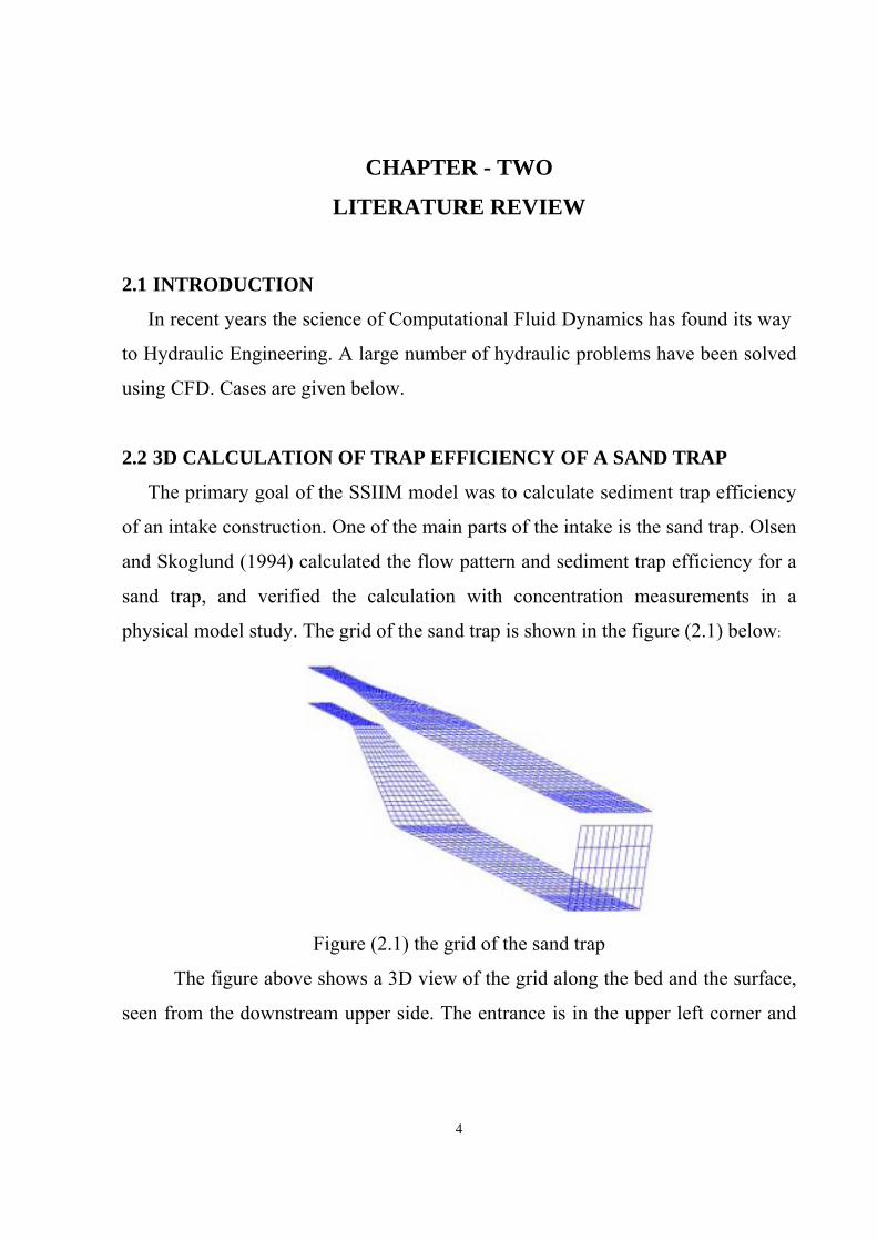
2.2 3D CALCULATION OF TRAP EFFICIENCY OF A SAND TRAP

The primary goal of the SSIIM model was to calculate sediment trap efficiency

of an intake construction. One of the main parts of the intake is the sand trap. Olsen

and Skoglund (1994) calculated the flow pattern and sediment trap efficiency for a

sand trap, and verified the calculation with concentration measurements in a

physical model study. The grid of the sand trap is shown in the figure (2.1) below:

Figure (2.1) the grid of the sand trap

The figure above shows a 3D view of the grid along the bed and the surface,

seen from the downstream upper side. The entrance is in the upper left corner and

5

the outlet in the lower right corner. There is an expansion region where the feeder

channel flows into the sand trap.

The figure (2.2) below shows the measured and calculated concentration

profiles in a longitudinal section. The lines are calculated concentrations and the

crosses are measured values. There is fairly good agreement between the calculated

and observed concentrations. [1]

Figure (2.2) the measured (x) and calculated concentration

2.3 SEDIMENT DEPOSITION AND BED MOVEMENTS IN A SAND TRAP

The original trap efficiency calculation for the sand trap in paragraph 2.2 was

for a steady situation. After some time, the sand trap will partly fill up with

sediments before it is flushed. It is of interest to predict how the trap efficiency

changes as the sand deposit. This requires calculation of the vertical bed

movements in the sand trap. Olsen and Kjellesvig (1999) calculated sediment

movements and bed changes in a tunnel- type sand trap. This was compared with

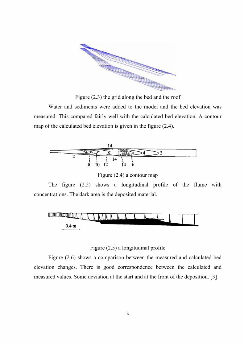
results from a physical model study. The figure (2.3) below shows a 3D views of

the grid along the bed and the roof. The upper left part of the figure is the entrance,

and the lower right part is the outlet.

6

Figure (2.3) the grid along the bed and the roof

Water and sediments were added to the model and the bed elevation was

measured. This compared fairly well with the calculated bed elevation. A contour

map of the calculated bed elevation is given in the figure (2.4).

Figure (2.4) a contour map

The figure (2.5) shows a longitudinal profile of the flume with

concentrations. The dark area is the deposited material.

Figure (2.5) a longitudinal profile

Figure (2.6) shows a comparison between the measured and calculated bed

elevation changes. There is good correspondence between the calculated and

measured values. Some deviation at the start and at the front of the deposition. [3]

7

Figure (2.6) Comparison between measured & calculated values

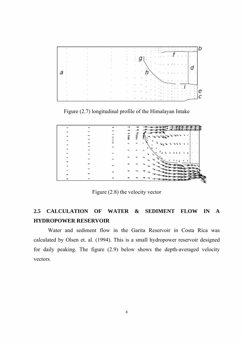
2.4 HIMALAYA INTAKE

An intake construction sometimes has a very complex geometry. One of the

most complex flow cases modeled with SSIIM was the Himalayan Intake. The

intake was designed by Prof. H. Støle as a mean of decreasing sediment problems

for run-of-the-river hydropower plants taking water from steep rivers. The

geometry of the CFD model was made by H. Kjellesvig (1995). (Kjellesvig and

Støle, 1996). The intake has gates both close to the surface and close to the bed.

This allows both floating debris and bed load to pass the intake dam. The dam itself

has a large intake in form of a tube, parallel to the dam axis. The longitudinal

profiles shown in Figure (2.7) are cross-sections of the dam and the tube and the

figure (2.8) shows the velocity vector of the dam. At the exit of this tube, the water

goes to the hydropower plant. Most of the water enters at the upper part of the tube,

where the sediment concentration is lowest. There is also an opening at the bottom

of the tube, allowing deposited sediments to fall down into the river and be flushed

out. [3]

8

Figure (2.7) longitudinal profile of the Himalayan Intake

Figure (2.8) the velocity vector

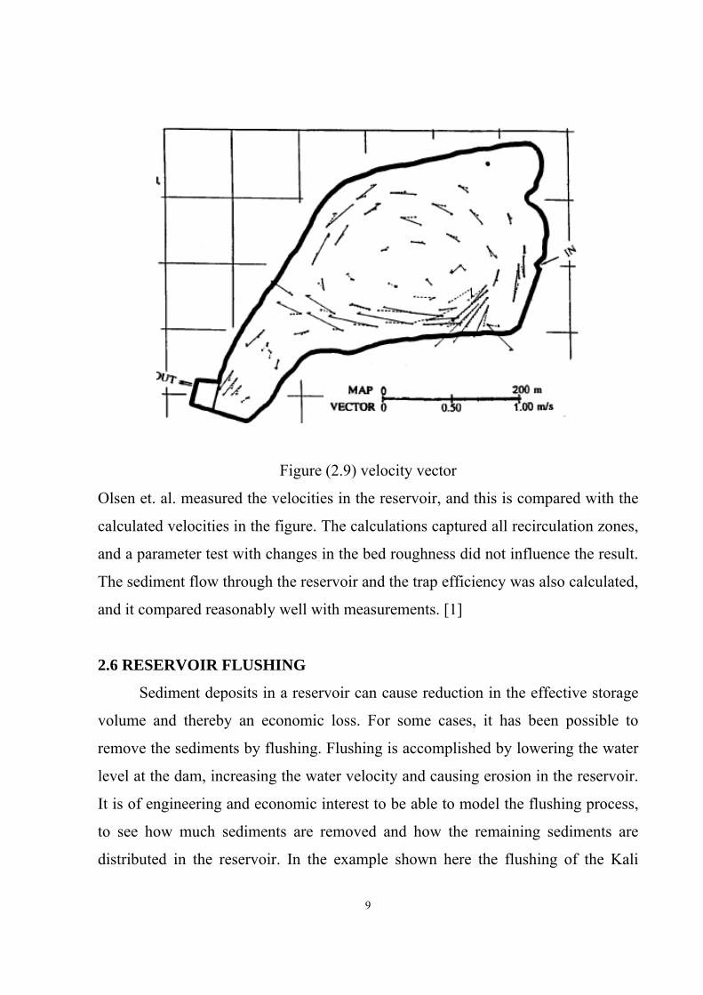
2.5 CALCULATION OF WATER & SEDIMENT FLOW IN A

HYDROPOWER RESERVOIR

Water and sediment flow in the Garita Reservoir in Costa Rica was

calculated by Olsen et. al. (1994). This is a small hydropower reservoir designed

for daily peaking. The figure (2.9) below shows the depth-averaged velocity

vectors.

9

Figure (2.9) velocity vector

Olsen et. al. measured the velocities in the reservoir, and this is compared with the

calculated velocities in the figure. The calculations captured all recirculation zones,

and a parameter test with changes in the bed roughness did not influence the result.

The sediment flow through the reservoir and the trap efficiency was also calculated,

and it compared reasonably well with measurements. [1]

2.6 RESERVOIR FLUSHING

Sediment deposits in a reservoir can cause reduction in the effective storage

volume and thereby an economic loss. For some cases, it has been possible to

remove the sediments by flushing. Flushing is accomplished by lowering the water

level at the dam, increasing the water velocity and causing erosion in the reservoir.

It is of engineering and economic interest to be able to model the flushing process,

to see how much sediments are removed and how the remaining sediments are

distributed in the reservoir. In the example shown here the flushing of the Kali

10

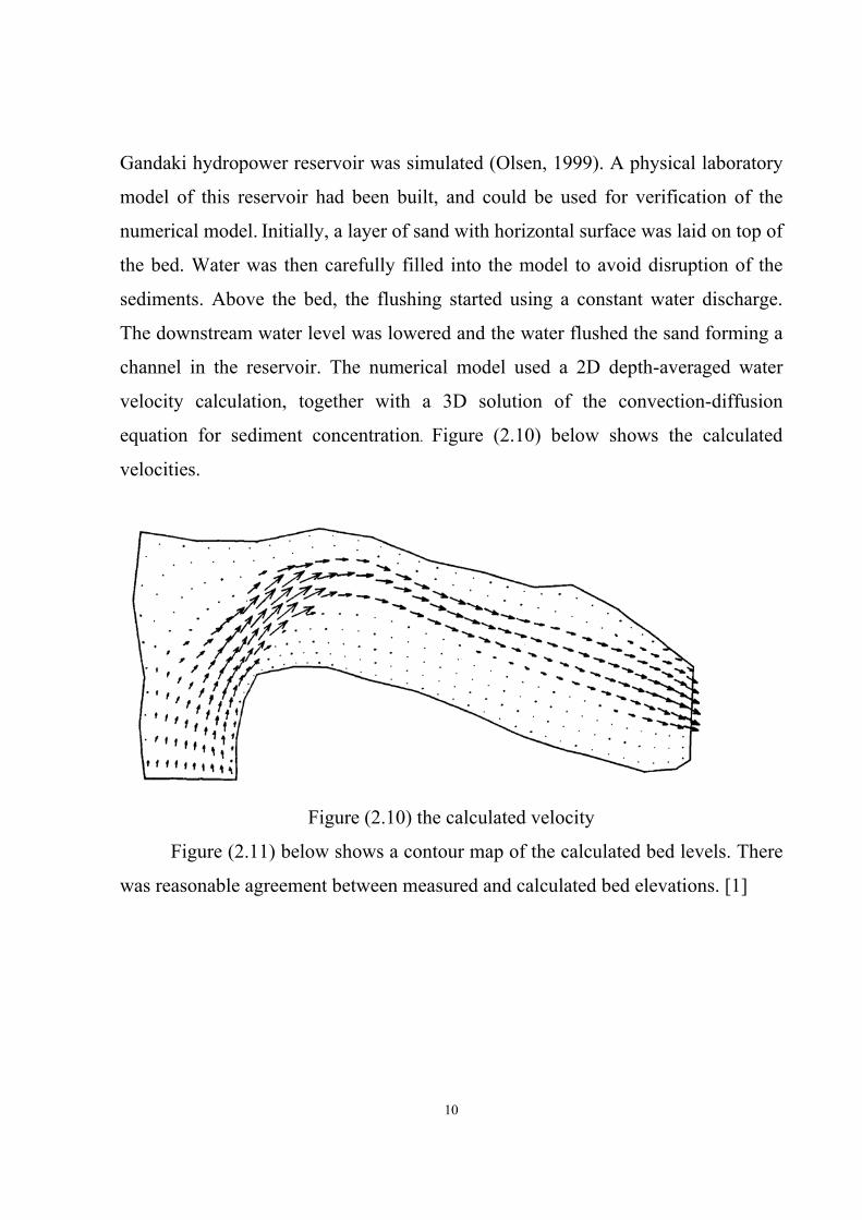
Gandaki hydropower reservoir was simulated (Olsen, 1999). A physical laboratory

model of this reservoir had been built, and could be used for verification of the

numerical model. Initially, a layer of sand with horizontal surface was laid on top of

the bed. Water was then carefully filled into the model to avoid disruption of the

sediments. Above the bed, the flushing started using a constant water discharge.

The downstream water level was lowered and the water flushed the sand forming a

channel in the reservoir. The numerical model used a 2D depth-averaged water

velocity calculation, together with a 3D solution of the convection-diffusion

equation for sediment concentration. Figure (2.10) below shows the calculated

velocities.

Figure (2.10) the calculated velocity

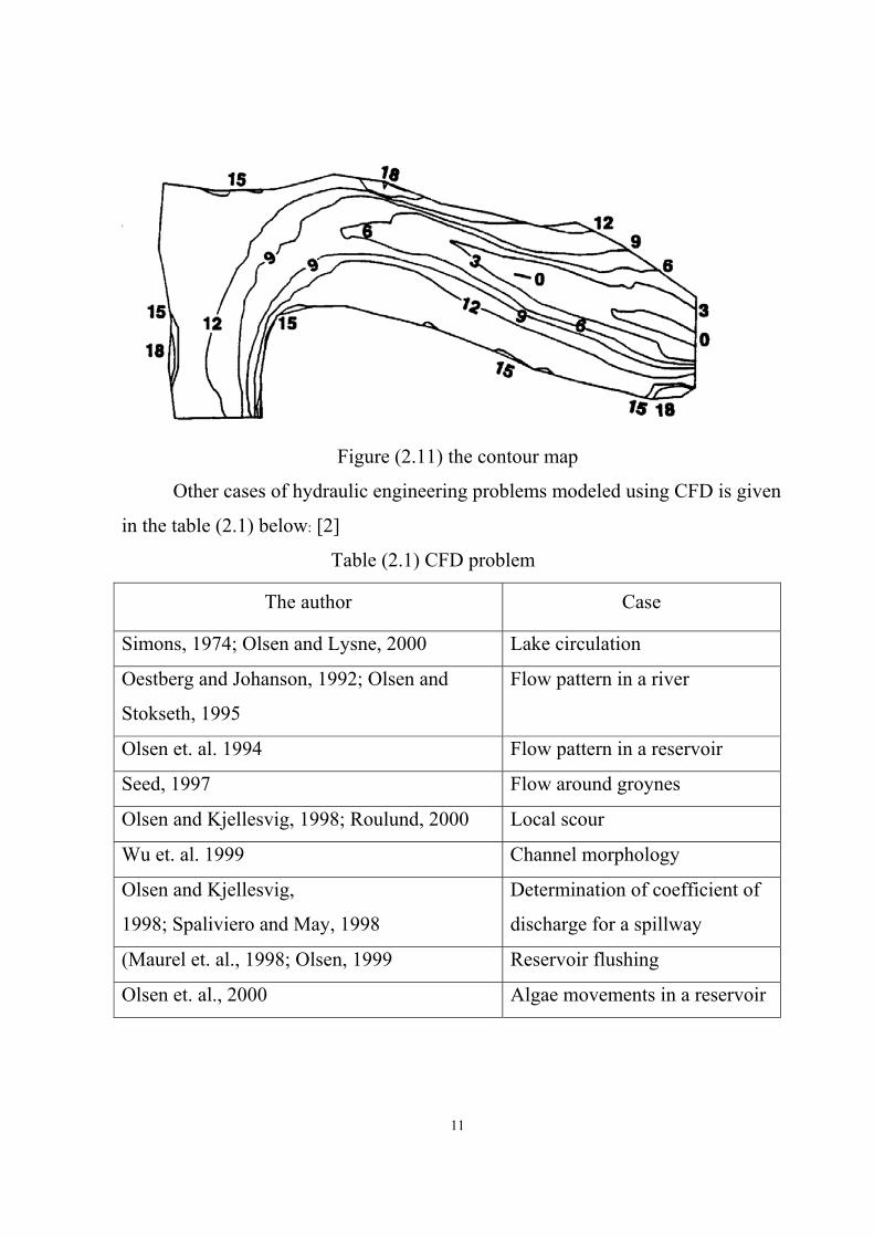
Figure (2.11) below shows a contour map of the calculated bed levels. There

was reasonable agreement between measured and calculated bed elevations. [1]

11

Figure (2.11) the contour map

Other cases of hydraulic engineering problems modeled using CFD is given

in the table (2.1) below: [2]

Table (2.1) CFD problem

The author Case

Simons, 1974; Olsen and Lysne, 2000 Lake circulation

Oestberg and Johanson, 1992; Olsen and

Stokseth, 1995

Flow pattern in a river

Olsen et. al. 1994 Flow pattern in a reservoir

Seed, 1997 Flow around groynes

Olsen and Kjellesvig, 1998; Roulund, 2000 Local scour

Wu et. al. 1999 Channel morphology

Olsen and Kjellesvig,

1998; Spaliviero and May, 1998

Determination of coefficient of

discharge for a spillway

(Maurel et. al., 1998; Olsen, 1999 Reservoir flushing

Olsen et. al., 2000 Algae movements in a reservoir

12

CHAPTER -THREE

SEDIMENT AND WATER FLOW CALCULATION

3.1 INTRODUCTION

Reservoir sedimentation is the process of sediment deposition into a lake

formed after a dam construction. A dam causes reduction in flow velocity and

consequently in turbulence, which causes a settling process of the materials carried

by the rivers. This is the mechanism that ultimately causes the sedimentation in

reservoirs which is a problem for their designers and users. Depending on the

amount of material deposited, the shortening of the reservoir useful lifetime will

bring several unpredicted consequences. The consequences of reservoir

sedimentation can be economically serious. A storage capacity loss in reservoirs

means financial losses due to the shortening of their useful lifetime. Beyond the

useful lifetime reduction, in reservoirs that are for hydropower generation, high

sediment load in the reservoir water may cause turbine abrasion. In flood detention

reservoirs, if the lake is filled up by sediments, floods cannot be detained and high

water levels downstream may cause high economic or even human life losses. The

reservoir sedimentation problem has increased worldwide year after year due to the

increase not only of the number of dams but also in their size. Approximately 1%

of the storage volume of the world’s reservoirs is lost annually due to sediment

deposition [8].

3.2 THE BLUE NILE RIVER:

The Blue Nile River is originating from the Ethiopian plateau, it shows very

high seasonal variation and it contains most highly devolved and productive

agriculture region in the Sudan (75% of national total area under irrigation

13

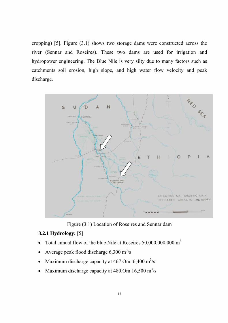
cropping) [5]. Figure (3.1) shows two storage dams were constructed across the

river (Sennar and Roseires). These two dams are used for irrigation and

hydropower engineering. The Blue Nile is very silty due to many factors such as

catchments soil erosion, high slope, and high water flow velocity and peak

discharge.

Figure (3.1) Location of Roseires and Sennar dam

3.2.1 Hydrology: [5]

• Total annual flow of the blue Nile at Roseires 50,000,000,000 m3

• Average peak flood discharge 6,300 m3/s

• Maximum discharge capacity at 467.Om 6,400 m3/s

• Maximum discharge capacity at 480.Om 16,500 m3/s

14

• Maximum recorded flood (60 years) 10,800 m3/s

• Average low river flow 100 m3/s.

3.3 ROSEIRES POWER STATION AND DAM:

Roseires power station and dam are located in Damazin approximately

500km. south of Khartoum, on the Blue Nile River. The dam is constructed in

1966 primary for irrigation purposes. Control and operation of the reservoir and

dam are totally vested in the ministry of irrigation. The power station, which was

commissioned about five years later, has a nameplate installed capacity of 130 MW

(3 turbine*30 MW+1*40) (as against a total system capacity of approximately 225

MW). The gross generation at Roseires in 1978 -1979 was 540, 385 MWH as

against a total system generation of 738, 269 MWH. It feeds into the system

through signal 220kv line which runs from Damazin to Khartoum. Work on

stringing of a second 220 kV line to Marignan on the same masts has commenced.

[For more details see [6].

3.3.1 Dam (first stage)

The dam is concrete buttress type about 1,000 m long, flanked on both side

by earth embankment, 8.5 Km long to the west and 4 Km long to the east. The deep

sluice structure is sited in the main river channel and contains five sluice ways

positioned as low as possible so that accumulations of silt in the reservoir can be

kept to minimum.

To the west of the deep sluice is the surface spillway controlled by seven

radial gates. Use to pass the peak of the load. During the peak of the flood all

spillway gates are kept fully open the deep sluice use to maintain the reservoir at

15

R.L 467 m if possible at this time any floating debris reaching the dam can be pass

down stream over the spillway. [5]

2.4 SEDIMENTATION ENGINEERING:

Sedimentation engineering is concerned with particle approaches to

investigation and solution of sediment problem involved in the development, use,

control, conservation of water and land resource. It is a serious problem if not well

through off. Sedimentation phenomenon can be created for or it happens due to:

• Soil erosion at upper reaches of catchment’s area

• Deforestation (Human influences )

• Hot dry spells which speeding up the erosion process

• Means of transporting weathered particles (Wind or water).

The phase describing the movement is complex, factors of influence are:

• Inflow discharge

• Velocity of flow

• Geometry of the channel

• The slope of the channel

• Bed material

• Operation process

3.4.1 Sedimentation Classification in Engineering Hydraulics:

Table (3.1) shows the British soil classification. There are other different

classifications worldwide but with small variations, specifically in the limits

between sand and silt and sand and gravel. [8]

16

Table (3.1) Sedimentation classification

Types Diameters range

Clay 2µm

Silt 2 to 60µm

Fine sand 60 to 200µm

Medium sand 200 to 600µm

Coarse sand 600 µm to 2mm

Gravel 2mm to 60mm

3.4.2 Siltation of the Blue Nile:

Silt transportation in the flood waters of the Blue Niles is a well known

phenomenon and has been the subject of many learned papers by eminent engineers

and scientists. The arrival of silt annually at Roseires conservatively estimated at

81*106 tones. The creation of reservoir at Roseires in 1966 provided a huge silt-

trap resulting in very rapid initial sedimentation. The Blue Nile posses the

necessary properties to carry sediment load such as:

• Ready source of silt originating mainly from severe erosion in the upper

catchments in Ethiopia and Sudan.

• Intensive rainfall in the upper reaches

• Steep gradients keep the silt in suspension ready to be deposition further

downstream.

• The sediment load of the Blue Nile amounts to 140 million ton/year.

• Part of this amount will be deposited in Roseires and Sennar dam reservoir

and minimizes their capacities.

17

3.4.3 Effect of the sediment:

• Need certain operations to keep certain upstream water level (minimize the

head)

• Minimize the head; means lower power generation, especially during peak

flows. (appendix A)

• Deposited sediment leads to the siltation of pumping station intake and

irrigation canals. Then leads to less water shortage and decreases crop

productivity.

• Fund is needed for desalting to restore original water level.

• Reduce the life time of the turbine parts (appendix B shows the parts cost

and damage cost).

• Height cost to remove the silt and high cost in MWH losses due to remove

(appendix C show the losses).

3.4.4 How to minimize the effect of sediment:

• Good watershed management over the whole catchments area to be enforced

to step down soil erosion.

• To carry out annual bathymetric survey to estimate the amount of deposited

sediment in order to choose the suitable process of desilting.

• Introduction of silt agitator to cut the sediment to be washed by water in the

main channel.

• To improve the current dredging process, this gave good result at Roseires

reservoir.

18

3.5 CALCULATION OF SEDIMENT TRANSPORT:

The following paragraphs describe methods to calculate suspended sediment

transport in a water flow. The same methods can be used to calculate other

parameters, for example water quality constituents, temperature etc. It is often

easier to understand the physics of the problem when the unknown variable is a

concentration of particles. Fluxes through cell surfaces are easier to understand

when one can imagine particles drifting with the water through the cell surfaces.

The transport processes are described first, and then the numerical algorithms are

described in the next chapter. Note that the numerical methods described in the

next chapter are also used for calculation of the water velocity field.

3.5.1 Transport processes

There are two main transport processes for suspended sediment transport:

convection and diffusion.

a. convective of sediment

The convection of sediments is the transport by the average water velocity.

The transport because of the fall velocity of the sediments is also a type of

convective transport. When calculating the flux, F, through a given surface with

area A, the following formula is used:

F = c * U * A ………………………………………………..(3.1)

U is the average velocity of the sediments normal to the surface, and c is the

average sediment concentration over the area. The sediment velocity will be the

sum of the water velocity and the sediment fall velocity. As an example, we can

look at a uniform flow, with zero vertical water velocity. If the surface is vertical,

the sediment fall velocity component is zero normal to the surface.

Then the velocity U will be equal to the horizontal water velocity. If the

surface is parallel to the bed/water surface, then the water velocity component

19

normal to the surface will be zero. The velocity U in equation (3.1) will then be

equal to the fall velocity of the sediment particles.

b. Diffusion of sediment:

The other process is the turbulent diffusion of sediments. This is due to

turbulent mixing and concentration gradients. The turbulent mixing process is

usually modelled with a turbulence mixing coefficient, Γ, defined as the sediment

flux divided by the concentration gradient: [1]

)2.3....(..........................................................................................⎟⎠⎞

⎜⎝⎛

⎟⎠⎞

⎜⎝⎛

=Γ

dxdcAF

Normally, the convective transport will be dominating. But in some cases, the

diffusive transport is important. An example is the reduced settling in a sand trap

because of turbulence.

3.5.2 The convection-diffusion equation

The convection-diffusion equation for steady sediment transport is: [1]

)3.3.....(..................................................⎟⎟⎠

⎞⎜⎜⎝

⎛

∂∂

Γ∂∂

=∂∂

+∂∂

jT

jjj x

cxz

cwxcU

The Einstein summation convention/tensor notation is used, meaning repeated

indexes are summed over all directions. For three-dimensional flow this means that

the equation can be written

)4.3.........(..........⎟⎠⎞

⎜⎝⎛

∂∂

Γ∂∂

+⎟⎟⎠

⎞⎜⎜⎝

⎛∂∂

Γ∂∂

+⎟⎠⎞

⎜⎝⎛

∂∂

Γ∂∂

=∂∂

+∂∂

+∂∂

+∂∂

zc

zyc

yxc

xzcw

zcW

ycV

xcU TTT

Equation (3.4) is used to describe the process of sediment transport.

20

3.5.3 Simple turbulence models

The turbulence model determines the value of the sediment concentration

diffusivity. The simplest turbulence model is the constant diffusivity model, when

the turbulent diffusivity is set constant throughout the computational domain. As an

example, a value of 1000 times the kinematics viscosity could be used. The

approach is fairly crude, but has nevertheless given reasonable results in some

cases. A better way to find the turbulent diffusivity for rivers is to use the following

formula:[1]

Γ = α U* H …………………………….………………………. (3.5)

The parameter α is an empirical constant. A value of 0.11 is often used.

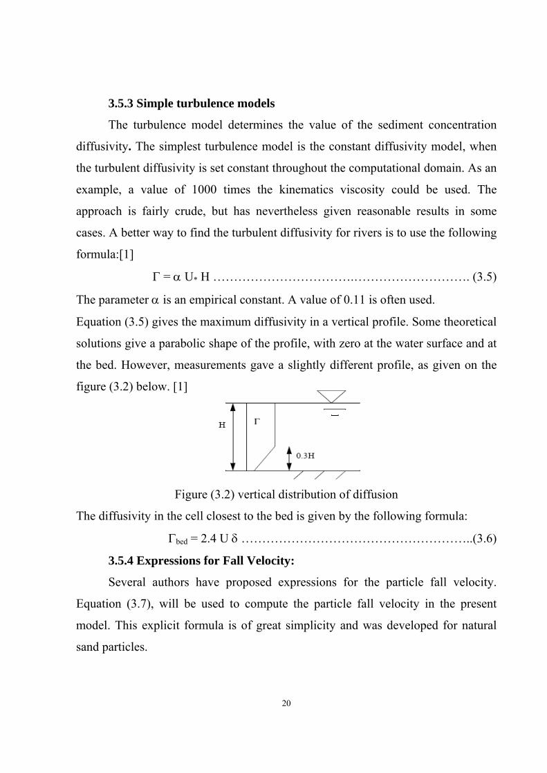
Equation (3.5) gives the maximum diffusivity in a vertical profile. Some theoretical

solutions give a parabolic shape of the profile, with zero at the water surface and at

the bed. However, measurements gave a slightly different profile, as given on the

figure (3.2) below. [1]

Figure (3.2) vertical distribution of diffusion

The diffusivity in the cell closest to the bed is given by the following formula:

Γbed = 2.4 U δ ………………………………………………..(3.6)

3.5.4 Expressions for Fall Velocity:

Several authors have proposed expressions for the particle fall velocity.

Equation (3.7), will be used to compute the particle fall velocity in the present

model. This explicit formula is of great simplicity and was developed for natural

sand particles.

21

( ) )7.3.(................................................................................5*2.1255.12

5050 −+= d

dws

υ

Where ws is the particle fall velocity, d50 is the sediment particle diameter finer than

50%, υ the fluid kinematic viscosity.

)8.3......(....................................................................................................50

31

2* dgd ⎟⎠⎞

⎜⎝⎛ ∆

=υ

Where ∆=(ρs-ρ)/ ρ. Cheng also compared his equation with previous studies and

found that his formula has a great degree of prediction accuracy.[8]

3.6 CALCULATION OF WATER VELOCITY:

This paragraph describes the solution procedures for the Navier-Stokes

equations. These equations describe the water velocity and turbulence in a river or

a hydraulic system.

3.6.1 Navier-Stokes equations

The Navier-Stokes equations describe the water velocity. The equations are

derived on the basis of equilibrium of forces on a small volume of water in laminar

flow. For turbulent flow, it is common to use the Reynolds’ averaged versions of

the equations. The Reynolds’ averaging is described first.

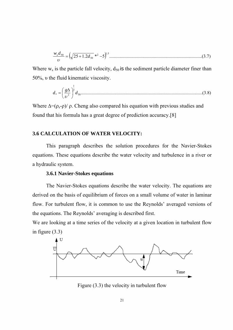
We are looking at a time series of the velocity at a given location in turbulent flow

in figure (3.3)

Figure (3.3) the velocity in turbulent flow

22

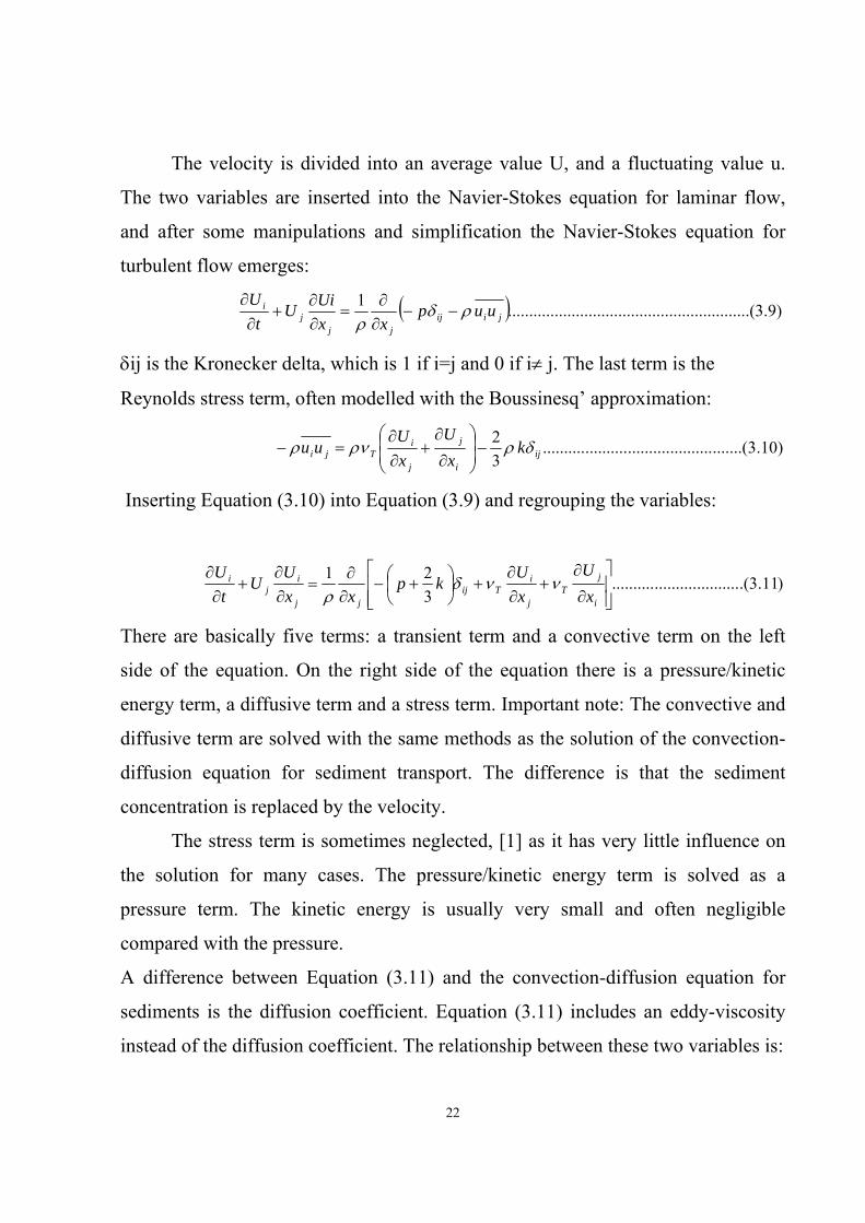
The velocity is divided into an average value U, and a fluctuating value u.

The two variables are inserted into the Navier-Stokes equation for laminar flow,

and after some manipulations and simplification the Navier-Stokes equation for

turbulent flow emerges:

( ) )9.3.......(..................................................1jiij

jjj

i uupxx

UiUt

Uρδ

ρ−−

∂∂

=∂∂

+∂

∂

δij is the Kronecker delta, which is 1 if i=j and 0 if i≠ j. The last term is the

Reynolds stress term, often modelled with the Boussinesq’ approximation:

)10.3.......(........................................32

iji

j

j

iTji k

xU

xU

uu δρρνρ −⎟⎟⎠

⎞⎜⎜⎝

⎛

∂

∂+

∂∂

=−

Inserting Equation (3.10) into Equation (3.9) and regrouping the variables:

)11.3.(..............................321

⎥⎥⎦

⎤

⎢⎢⎣

⎡

∂

∂+

∂∂

+⎟⎠⎞

⎜⎝⎛ +−

∂∂

=∂∂

+∂

∂

i

jT

j

iTij

jj

ij

i

xU

xU

kpxx

UU

tU

ννδρ

There are basically five terms: a transient term and a convective term on the left

side of the equation. On the right side of the equation there is a pressure/kinetic

energy term, a diffusive term and a stress term. Important note: The convective and

diffusive term are solved with the same methods as the solution of the convection-

diffusion equation for sediment transport. The difference is that the sediment

concentration is replaced by the velocity.

The stress term is sometimes neglected, [1] as it has very little influence on

the solution for many cases. The pressure/kinetic energy term is solved as a

pressure term. The kinetic energy is usually very small and often negligible

compared with the pressure.

A difference between Equation (3.11) and the convection-diffusion equation for

sediments is the diffusion coefficient. Equation (3.11) includes an eddy-viscosity

instead of the diffusion coefficient. The relationship between these two variables is:

23

Where Sc is the Schmidt number. This is usually set to unity, meaning that the

eddy-viscosity is the same as the turbulent sediment diffusivity.

This leaves the problem of solving the pressure term. Several methods exist,

but with the control volume approach, the most commonly used method is the

SIMPLE method.

3.6.2 The SIMPLE method

SIMPLE is an abbreviation for Semi-Implicit Method for Pressure-Linked

Equations. [1].The purpose of the method is to find the unknown pressure field.

The main idea is to guess a value for the pressure and use the continuity defect to

obtain an equation for a pressure-correction. When the pressure-correction is added

to the pressure, water continuity is satisfied. To derive the equations for the

pressure-correction, a special notation is used. The initially calculated variables do

not satisfy continuity and are denoted with an index *. The correction of the

variables is denoted with an index ‘. The variables after correction do not have a

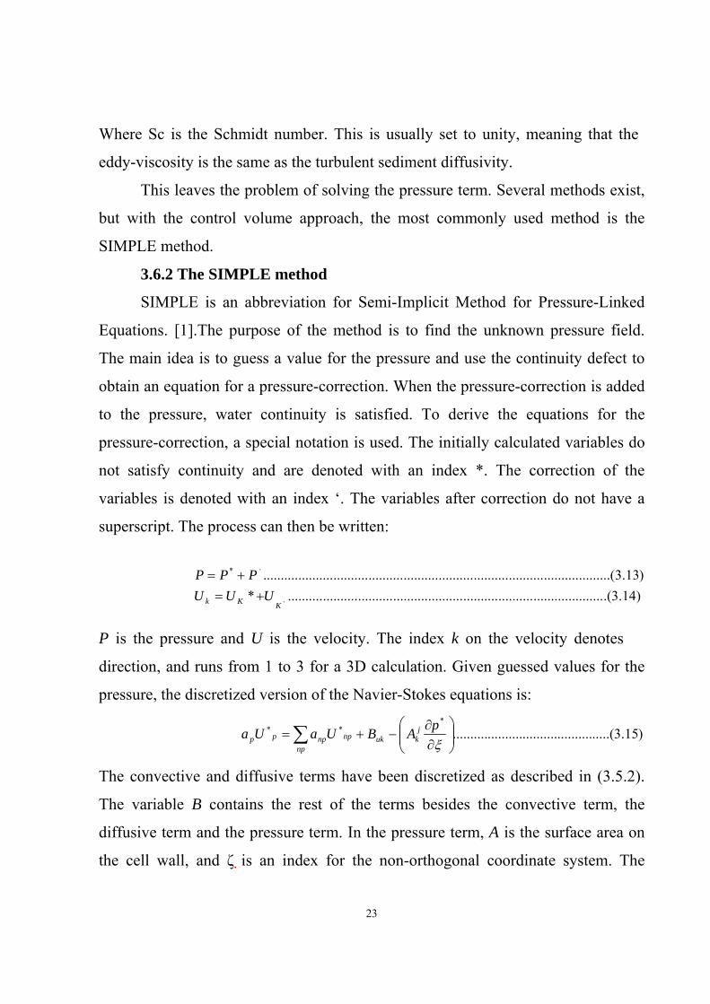
superscript. The process can then be written:

P is the pressure and U is the velocity. The index k on the velocity denotes

direction, and runs from 1 to 3 for a 3D calculation. Given guessed values for the

pressure, the discretized version of the Navier-Stokes equations is:

∑ ⎟⎟⎠

⎞⎜⎜⎝

⎛∂∂

−+=np

jkuknpnppp

pABUaUa )15.3.....(........................................*

**

ξ

The convective and diffusive terms have been discretized as described in (3.5.2).

The variable B contains the rest of the terms besides the convective term, the

diffusive term and the pressure term. In the pressure term, A is the surface area on

the cell wall, and ζ is an index for the non-orthogonal coordinate system. The

)14.3.(..........................................................................................*)13.3.........(..........................................................................................

,

,*

KKk UUUPPP

+=+=

24

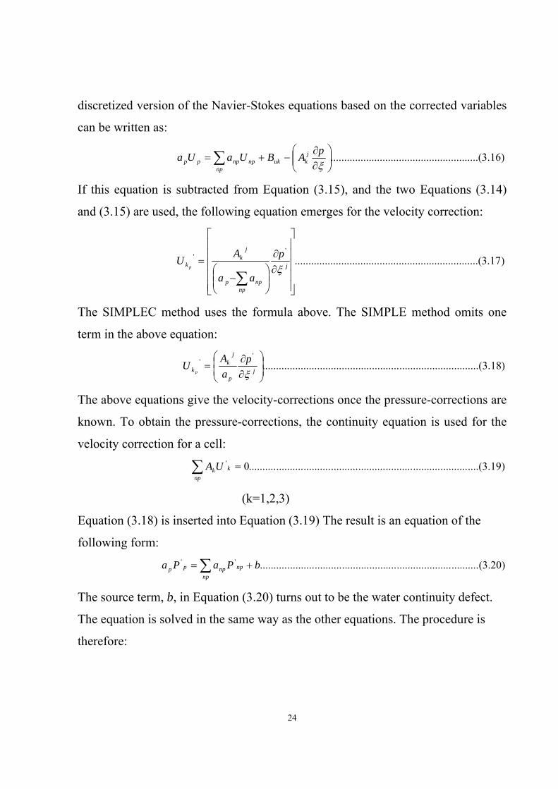
discretized version of the Navier-Stokes equations based on the corrected variables

can be written as:

∑ ⎟⎟⎠

⎞⎜⎜⎝

⎛∂∂

−+=np

jkuknpnppp

pABUaUa )16.3....(..................................................ξ

If this equation is subtracted from Equation (3.15), and the two Equations (3.14)

and (3.15) are used, the following equation emerges for the velocity correction:

)17.3.......(............................................................'

'

⎥⎥⎥⎥⎥

⎦

⎤

⎢⎢⎢⎢⎢

⎣

⎡

∂∂

⎟⎟⎠

⎞⎜⎜⎝

⎛−

=

∑j

npnpp

jk

kp

aa

AU

p ξ

The SIMPLEC method uses the formula above. The SIMPLE method omits one

term in the above equation:

)18.3.........(......................................................................'

'

⎟⎟⎠

⎞⎜⎜⎝

⎛

∂∂

= jp

jk

kp

aA

Up ξ

The above equations give the velocity-corrections once the pressure-corrections are

known. To obtain the pressure-corrections, the continuity equation is used for the

velocity correction for a cell:

)19.3....(................................................................................0'∑ =np

kkUA

(k=1,2,3)

Equation (3.18) is inserted into Equation (3.19) The result is an equation of the

following form:

∑ +=np

npnppp bPaPa )20.3(................................................................................''

The source term, b, in Equation (3.20) turns out to be the water continuity defect.

The equation is solved in the same way as the other equations. The procedure is

therefore:

25

1. Guess a pressure field, P*

2. Calculate the velocity U* by solving Equation (3.15)

3. Solve equation (3.20) and obtain the pressure-correction, P’

4. Correct the pressure by adding P’ to P*

5. Correct the velocities U* with U’ using equation (3.18)

6. Restart calculation from step 2 to find a converged solution

An equation for the pressure is not solved directly, only an equation for the

pressure correction. The pressure is obtained by accumulative addition of the

pressure-correction values. The SIMPLE method can give instabilities when

calculating the pressure field. Therefore, the pressure-correction is often multiplied

with a number below unity before being added to the pressure. The number is a

relaxation coefficient. The value 0.2 is often used. The optimum factor depends on

the flow situation and can be changed to give better convergence rates.

Regarding the difference between the SIMPLE and the SIMPLEC method, the

SIMPLEC should be more consistent in theory, as a more correct formula is used.

Looking at Equations (3.17) and (3.18), the SIMPLE method will give a lower

correction than the SIMPLEC method, as the denominator will be larger. The

SIMPLE method will therefore move slower towards convergence than the

SIMPLEC method. If there are problems with instabilities, this can be an

advantage.

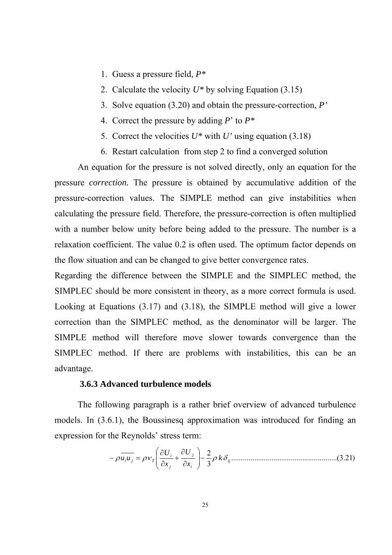
3.6.3 Advanced turbulence models

The following paragraph is a rather brief overview of advanced turbulence

models. In (3.6.1), the Boussinesq approximation was introduced for finding an

expression for the Reynolds’ stress term:

)21.3.....(..................................................32

iji

j

j

iTji k

xU

xU

uu δρρνρ −⎟⎟⎠

⎞⎜⎜⎝

⎛

∂

∂+

∂∂

=−

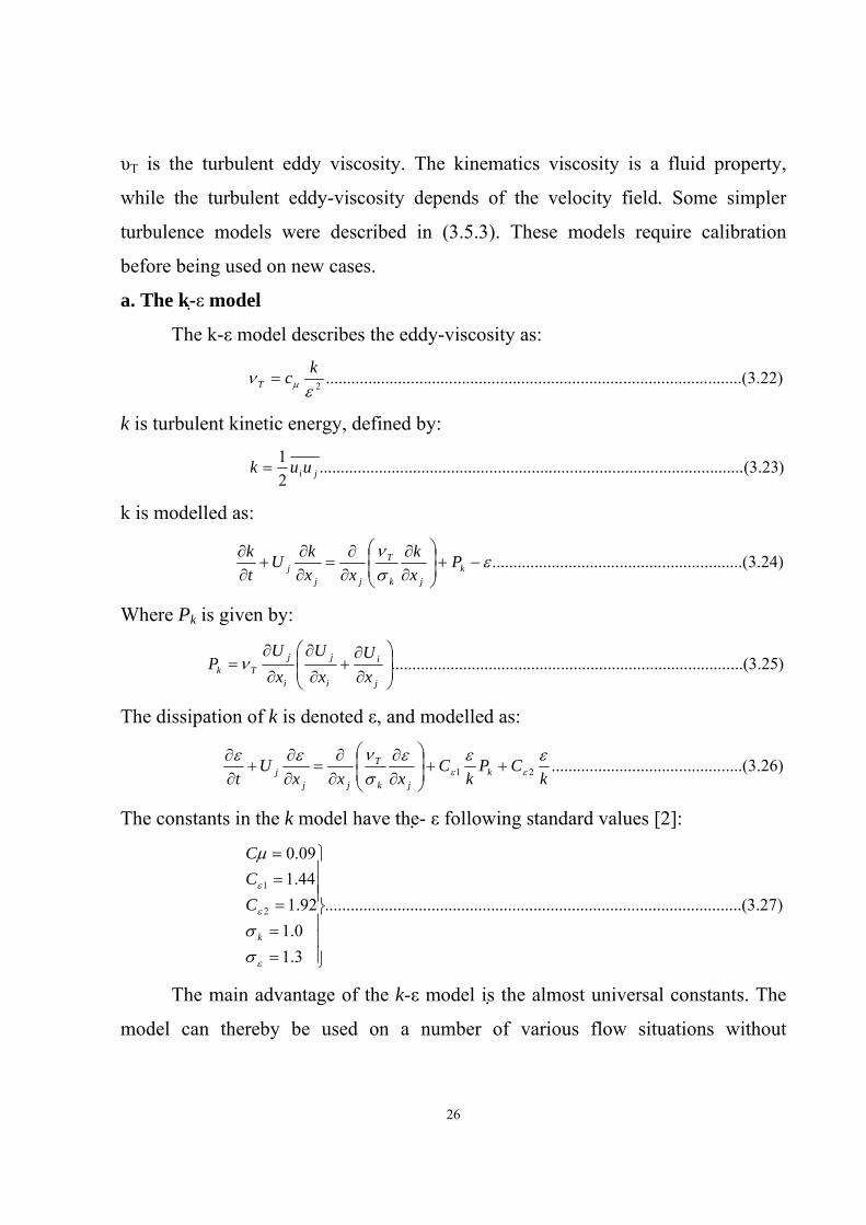
26

υT is the turbulent eddy viscosity. The kinematics viscosity is a fluid property,

while the turbulent eddy-viscosity depends of the velocity field. Some simpler

turbulence models were described in (3.5.3). These models require calibration

before being used on new cases.

a. The k- ε model

The k-ε model describes the eddy-viscosity as:

)22.3........(..........................................................................................2εν µ

kcT =

k is turbulent kinetic energy, defined by:

)23.3(....................................................................................................21

jiuuk =

k is modelled as:

)24.3.........(..................................................εσν

−+⎟⎟⎠

⎞⎜⎜⎝

⎛

∂∂

∂∂

=∂∂

+∂∂

kjk

T

jjj P

xk

xxkU

tk

Where Pk is given by:

)25.3...(................................................................................⎟⎟⎠

⎞⎜⎜⎝

⎛

∂∂

+∂

∂

∂

∂=

j

i

i

j

i

jTk x

Ux

Ux

UP ν

The dissipation of k is denoted ε, and modelled as:

)26.3.....(........................................21 kCP

kC

xxxU

t kjk

T

jjj

εεεσνεε

εε ++⎟⎟⎠

⎞⎜⎜⎝

⎛

∂∂

∂∂

=∂∂

+∂∂

The constants in the k model have the- ε following standard values [2]:

)27.3........(..........................................................................................

3.10.192.144.109.0

2

1

⎪⎪⎪

⎭

⎪⎪⎪

⎬

⎫

=====

ε

ε

ε

σσ

µ

k

CCC

The main advantage of the k-ε model is the almost universal constants. The

model can thereby be used on a number of various flow situations without

27

calibration. For river engineering this may not always be the case, because when

friction along the bed is influencing the flow field, the roughness of the bed also

needs to be given. If the roughness can not be obtained from direct measurements,

it has to be calibrated with measurements of the velocity. As seen from Equation

(3.21), the eddy-viscosity is isotropic, and modelled as an average for all three

directions. Several authors investigated the eddy-viscosity in a laboratory flume in

three directions. His work shows that the eddy-viscosity in the stream wise

direction is almost one magnitude greater than in the cross-stream wise direction

[2]. A better turbulence model could therefore give more accurate results for many

cases.

b. More advanced turbulence models

To be able to model non-isotropic turbulence, a more accurate representation

of the Reynolds stress is needed. Instead of using the Boussinesq approximation

(Equation 3.19), the Reynolds’ stress can be modelled with all terms.

)28.3....(..................................................⎥⎥⎥

⎦

⎤

⎢⎢⎢

⎣

⎡

−=−wwvwuwwvvvuvvuvuuu

uu ji ρρ

The following notation is used: u is the fluctuating velocity in direction 1, v

is the fluctuating velocity in direction 2 and w is the fluctuating velocity in

direction 3. The nine terms shown on the right hand side of Equation (3.28) can be

condensed into six different terms, as the matrix is symmetrical. A Reynolds’ stress

model will solve an equation for each of the six unknown terms. Usually,

differential equations for each term are solved. This means that six differential

equations are solved compared with two for the k model. It means added

complexity and computational time. An - ε alternative is to use an Algebraic Stress

Model (ASM), where algebraic expressions for the various terms are used. It is also

possible to combine the k- model with an ASM to obtain non-isotropic eddy

28

viscosity [1]. An even more advanced method is to resolve the larger eddies with a

very fine grid, and use a turbulence model only for the smaller scales. This is called

Large-Eddy Simulation (LES). If the grid is so fine that sub-grid eddies doing not

exist because they are dissipated by the kinematics viscosity, the method is called a

Direct Solution (DS) of the Navier Stokes equations. Note that both LES and

especially DS modelling require extreme computational resources, which presently

is not feasible for engineering purposes.

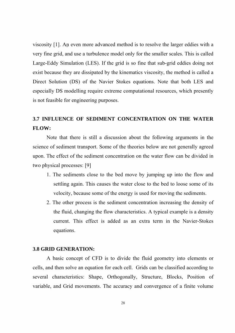
3.7 INFLUENCE OF SEDIMENT CONCENTRATION ON THE WATER

FLOW:

Note that there is still a discussion about the following arguments in the

science of sediment transport. Some of the theories below are not generally agreed

upon. The effect of the sediment concentration on the water flow can be divided in

two physical processes: [9]

1. The sediments close to the bed move by jumping up into the flow and

settling again. This causes the water close to the bed to loose some of its

velocity, because some of the energy is used for moving the sediments.

2. The other process is the sediment concentration increasing the density of

the fluid, changing the flow characteristics. A typical example is a density

current. This effect is added as an extra term in the Navier-Stokes

equations.

3.8 GRID GENERATION:

A basic concept of CFD is to divide the fluid geometry into elements or

cells, and then solve an equation for each cell. Grids can be classified according to

several characteristics: Shape, Orthogonally, Structure, Blocks, Position of

variable, and Grid movements. The accuracy and convergence of a finite volume

29

calculation depends on the quality of the grid. Three grid characteristics are

important non-Orthogonality, aspect ratio and expansion ratio. When drawing the

grid, the following points should be kept in mind:

1. The grid lines should follow the stream lines as much as possible

2. The grid line intersections should be as orthogonal as possible

3. The grid aspect ratio should not be too great

4. The grid expansion ratio should not be too great

5. There should be higher grid densities in areas with high

velocity/concentration

An out blocked region is a part of the grid where water is not allowed to flow. It

can be used for making islands or obstacles in the flow.

3.8.1 Grid Qualities

The accuracy and convergence of a finite volume calculation depends on the

quality of the grid. Three grid characteristics are important non-orthogonality,

aspect ratio and expansion ratio.

The non-orthogonality of the grid line intersections is the deviation from 90

degrees. If the grid line intersection is below 45 degrees or over 135 degrees, the

grid is said to be very non-orthogonal. This is a situation one should avoid. Low

non-orthogonality of the grid leads to more rapid convergence, and in some cases

better accuracy .The aspect ratio and expansion ratio is described in the figure (3.4)

below: The figure shows two grid cells, A and B. The lengths of the cells are ∆xA

and ∆xB.

Figure (3.4) Expansion/aspect ratio

∆yA

30

The expansion ratio of the grid at these cells is ∆xA/∆xB. The aspect ratio

of the grid at cell A is ∆xA/∆yA. The expansion ratio and the aspect ratio of a grid

should not be too great, in order to avoid convergence problems and inaccuracies.

Aspect ratios of 2-3 should not be a problem if the flow direction is parallel to the

longest side of the cell. Experience shows that aspect ratios of 10-50 will give

extremely slow convergence for water flow calculations. Expansion ratios under

1.2 will not pose problems for the solution. Experience also shows that expansion

ratios of around 10 can give very unphysical results for the water flow calculation.

3.9 BOUNDARY CONDITIONS:

Boundary conditions are required on all boundaries for the sediment flow

calculation. The two most used types of boundary conditions are:

• Zero gradients

• Dirichlet

Zero gradient boundary conditions means the derivative of the variable at the

boundary is zero. In other words, the value at the boundary is the same as the value

in the cell closest to the boundary. This boundary condition is often used at the

outflow boundary for the sediment concentration calculation. It can also be used at

walls.

Dirichlet boundary conditions means the values of a variable is given at the

boundary. For example, zero sediment concentration is usually set at the water

surface. Also, at the upstream boundary the sediment concentration has to be given.

One of the most challenging problems is the boundary condition for the sediment

concentration at the bed. For a general calculation, the sediments should be able to

both settle and erode, depending on the shear stress at the bed, the sediment particle

size distribution, the in and outflow of sediments from a section and the availability

of sediments for erosion. This can be done in two ways:

31

i. Define a pick-up rate of sediments where erosion occurs.

ii. Use an equilibrium concentration in the cell close to the bed.

Method (ii) is used in the SSIIM program, so this is further described in the

following text. The theory of equilibrium concentration at the bed was first

described by Einstein (1950), in his formula for sediment transport. The method

has since then been expanded by Toffalletti, and the latest contribution is from van

Rijn (1987). Van Rijn made a formula for the equilibrium concentration at the bed:

)29.3.........(................................................................................015.0 3.0*

5.150

DT

ad

c =

The parameter a is the distance from the concentration point to the bed, the

mean sediment particle diameter is denoted d50, T = (τ- τc)/ τ, where τ is the shear

stress, τc is the critical shear stress for movements of sediment particles, and D* is

given by:

)30.3.(....................................................................................................250* ⎥⎦

⎤⎢⎣

⎡ −=

vdD

w

ws

ρρρ

Here, ρs is the density of the sediment; ρw is the density of water and υ is the

kinematics viscosity of water. This formula is used in the cells close to the bed, as a

boundary condition at the bed.

3.9.1 Navier-Stock equation:

Boundary conditions for the Navier-Stokes equations are in many ways

similar to the solution of the convection-diffusion equation. In the following text, a

division in four parts is made: Inflow, outflow, water surface and bed/wall.

In the Inflow Dirichlet boundary conditions have to be given at the inflow

boundary. This is relatively straightforward for the velocities. Usually it is more

difficult to specify the turbulence. It is then possible to use a simple turbulence

32

model, to specify the eddy-viscosity. Given the velocity, it is also possible to

estimate the shear stress at the entrance bed. Then the turbulent kinetic energy k at

the inflow bed is determined by the following equation:

)31.3.....(..............................................................................................................µρ

τc

k =

This equation is based on equilibrium between production and dissipation of

turbulence at the bed cell. Given the eddy-viscosity and k at the bed, Equation

(3.22) gives the value of ε at the bed. If k is assumed to vary linearly from the bed

to the surface, with for example half the bed value at the surface, Equation (3.22)

can be used together with the profile of the eddy-viscosity to calculate the vertical

distribution of ε.

In the Outflow Zero gradient boundary conditions can be used at outflow

boundaries for all variables.

In the Water surface Zero gradient boundary conditions are used for ε. The

turbulent kinetic energy, k, is set to zero. Symmetrical boundary conditions are

used for the water velocity, meaning zero gradient boundary conditions are used for

the velocities in the horizontal directions. The velocity in the vertical direction is

calculated from the criteria of zero water flux across the water surface.

In the Bed/wall the flux through the bed/wall is zero, so no boundary

conditions are given. However, the flow gradient towards the wall is very steep,

and it would require a significant number of grid cells to dissolve the gradient

sufficiently. Instead, a wall law is used, transformed by integrating it over the cell

closest to the bed. Using a wall law for rough boundaries (Schlichting, 1980)

)32.3.........(....................................................................................................30ln1

*⎟⎟⎠

⎞⎜⎜⎝

⎛=

sky

kuU

33

Also takes the effect of the roughness, ks, on the wall into account. The velocity is

denoted U, u* is the shear velocity, ks is a coefficient equal to 0.4 and y is the

distance from the wall to the centre of the cell. The wall law is used both for the

velocities and the turbulence parameters.

3.10 DISCRETIZATION METHODS

The discretization described here is by the control volume method. The main

point of the discretization is: To transform the partial differential equation into a

new equation where the variable in one cell is a function of the variable in the

neighbour cells. The new function can be thought of as a weighted average of the

concentration in the neighbouring cells. For a two-dimensional situation, the

following notation is used, according to directions north, south, east and west:

Figure (3.4) two dimensional cells

cn concentration in cell n

ce concentration in cell e

cs concentration in cell s

cw concentration in cell w

cp concentration in cell p

ae: weighting factor for cell e

aw: weighting factor for cell w

an: weighting factor for cell n

as: weighting factor for cell s

34

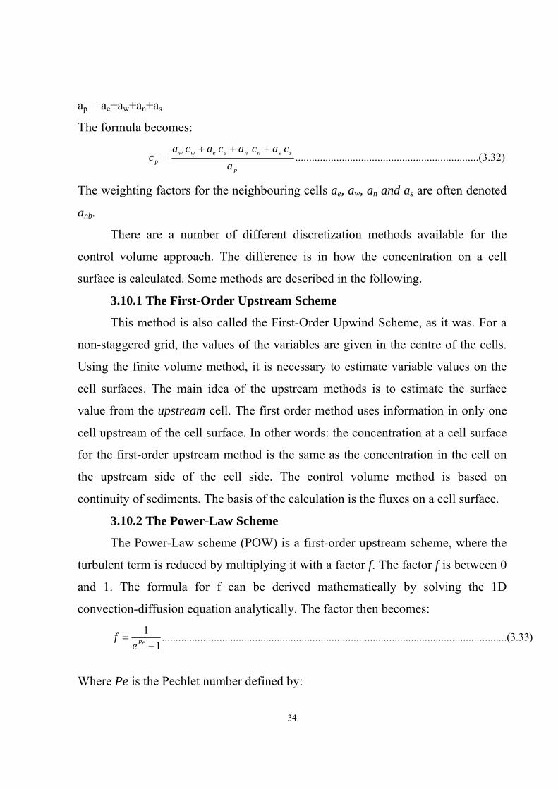
ap = ae+aw+an+as

The formula becomes:

)32.3.......(............................................................p

ssnneewwp a

cacacacac

+++=

The weighting factors for the neighbouring cells ae, aw, an and as are often denoted

anb.

There are a number of different discretization methods available for the

control volume approach. The difference is in how the concentration on a cell

surface is calculated. Some methods are described in the following.

3.10.1 The First-Order Upstream Scheme

This method is also called the First-Order Upwind Scheme, as it was. For a

non-staggered grid, the values of the variables are given in the centre of the cells.

Using the finite volume method, it is necessary to estimate variable values on the

cell surfaces. The main idea of the upstream methods is to estimate the surface

value from the upstream cell. The first order method uses information in only one

cell upstream of the cell surface. In other words: the concentration at a cell surface

for the first-order upstream method is the same as the concentration in the cell on

the upstream side of the cell side. The control volume method is based on

continuity of sediments. The basis of the calculation is the fluxes on a cell surface.

3.10.2 The Power-Law Scheme

The Power-Law scheme (POW) is a first-order upstream scheme, where the

turbulent term is reduced by multiplying it with a factor f. The factor f is between 0

and 1. The formula for f can be derived mathematically by solving the 1D

convection-diffusion equation analytically. The factor then becomes:

)33.3......(........................................................................................................................1

1−

= Peef

Where Pe is the Pechlet number defined by:

35

Pe = ρUL/Г

L is the length of the cell.

3.10.3 The Second Order Upstream Scheme

The Second-Order Upstream (SOU) method is based on a second-order

accurate method to calculate the concentration on the cell surfaces. The method

only involves the convective fluxes

36

CHAPTER - FOUR

SOFTWARE

4.1 SSIIM PROGRAM

SSIIM is an abbreviation of Sediment Simulation in Intakes with Multiblock

option. The program is made for use in hydraulic and sedimentation engineering. It

is based on the control volume approach with a 3D structured non-orthogonal grid.

The Navier Stokes equations are solved, and also the convection-diffusion equation

for sediment transport. SSIIM has been used in a number of studies relating to

water flow and sediment transport in river and hydropower engineering. This

includes trap efficiency of sand traps and hydropower reservoirs, turbidity currents,

erosion and local scour, flood waves, head loss and spillways.

4.2 MODEL OVERVIEW

The SSIIM program solves the Navier-Stokes equations with the k-ε model

on a three-dimensional almost general non-orthogonal grid. A control volume

method is used for the discretization, together with the power-law scheme or the

second order upwind scheme. The SIMPLE method is used for the pressure

coupling. An implicit solver is used, producing the velocity field in the geometry.

The velocities are used when solving the convection-diffusion equations for

different sediment sizes. This gives trap efficiency and sediment deposition pattern.

The user interface of the program can present velocity vectors and scalar variables

in a two dimensional view of the three-dimensional grid, in plan view, a cross-

section or a longitudinal profile. The model includes several utilities facilitating the

creation of input data. Some data can be given in dialog boxes. There is also an

37

interactive graphical grid editor with elliptic and transfinite interpolation together

with a discharge editor

4.3 MODEL PURPOSE

The program is made for use in River/ Environmental/ Hydraulic/

Sedimentation Engineering. Initially, the main motivation for creating the program

was to simulate the sediment movements in general river/channel geometries. This

has shown to be difficult to do in physical model studies for fine sediments. Later,

the use of the program has been extended to other hydraulic engineering topics, for

example spillway modelling, head loss in tunnels, stage-discharge relationships in

rivers, turbidity currents and the main strength of SSIIM compared to other CFD

program is the capability of modelling sediment transport with moveable bed in a

complex geometry. This includes multiple sediment sizes, sorting, bed load and

suspended load, bed forms and effects of sloping beds. The latest module for

wetting and drying in the unstructured grid further enables complex

geomorphological modelling. Over the years, SSIIM has also been used for habitat

studies in rivers, mainly for salmon. In the last years, free-flowing algae have also

been modelled, as a part of extending the model for use in water quality

engineering. However, the main focus of our research is on sediment transport.

4.4 LIMITATION OF THE PROGRAM

SSIIM for OS/2 requires OpenGL graphics libraries to be installed with the

operating system. These are included in OS/2 version 4.0 and later. The OpenGL

graphics for Windows will run on Windows NT and Windows 2000. It may not run

on Windows 95 or Windows 98. Some of the limitations of the program are listed

below.

38

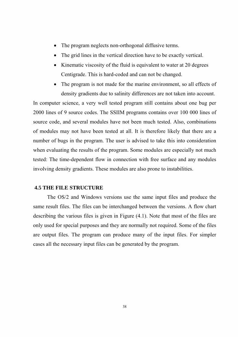
• The program neglects non-orthogonal diffusive terms.

• The grid lines in the vertical direction have to be exactly vertical.

• Kinematic viscosity of the fluid is equivalent to water at 20 degrees

Centigrade. This is hard-coded and can not be changed.

• The program is not made for the marine environment, so all effects of

density gradients due to salinity differences are not taken into account.

In computer science, a very well tested program still contains about one bug per

2000 lines of 9 source codes. The SSIIM programs contains over 100 000 lines of

source code, and several modules have not been much tested. Also, combinations

of modules may not have been tested at all. It is therefore likely that there are a

number of bugs in the program. The user is advised to take this into consideration

when evaluating the results of the program. Some modules are especially not much

tested: The time-dependent flow in connection with free surface and any modules

involving density gradients. These modules are also prone to instabilities.

4.5 THE FILE STRUCTURE

The OS/2 and Windows versions use the same input files and produce the

same result files. The files can be interchanged between the versions. A flow chart

describing the various files is given in Figure (4.1). Note that most of the files are

only used for special purposes and they are normally not required. Some of the files

are output files. The program can produce many of the input files. For simpler

cases all the necessary input files can be generated by the program.

39

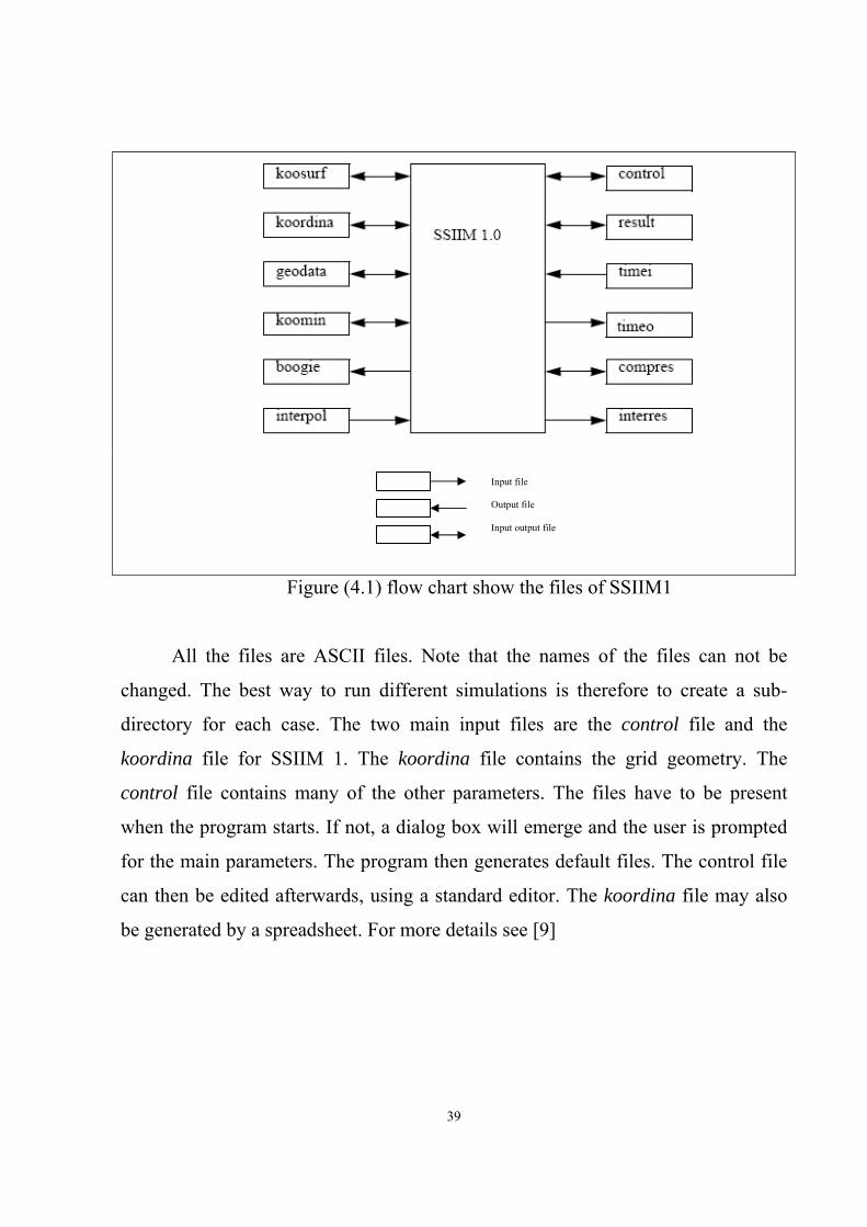
Figure (4.1) flow chart show the files of SSIIM1

All the files are ASCII files. Note that the names of the files can not be

changed. The best way to run different simulations is therefore to create a sub-

directory for each case. The two main input files are the control file and the

koordina file for SSIIM 1. The koordina file contains the grid geometry. The

control file contains many of the other parameters. The files have to be present

when the program starts. If not, a dialog box will emerge and the user is prompted

for the main parameters. The program then generates default files. The control file

can then be edited afterwards, using a standard editor. The koordina file may also

be generated by a spreadsheet. For more details see [9]

Input file Output file Input output file

40

4.6 MODELLING COMPLEX STRUCTURES WITH SSIIM

Often, a hydraulic structure is best modelled by SSIIM 1. This is because of

its outblocking options and the possibility to create walls along grid lines. A

hydraulic structure often has vertical walls with channel openings, and this is

problematic to model for SSIIM 2. The outblocked areas are modelled in the

control file, by changing the G 13 data sets (For more information about all data

sets see [9]). The walls between cells are modelled with the W 4 data set. [3]

4.7 PROBLEM SETUP

We take three dimensional models from Rosaries reservoir before the dam

according to

4.7.1 Geometry

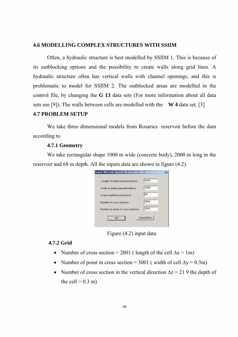
We take rectangular shape 1000 m wide (concrete body), 2000 m long in the

reservoir and 68 m depth. All the inputs data are shown in figure (4.2).

Figure (4.2) input data

4.7.2 Grid

• Number of cross section = 2001 ( length of the cell ∆x = 1m)

• Number of point in cross section = 3001 ( width of cell ∆y = 0.3m)

• Number of cross section in the vertical direction ∆z = 21 9 the depth of

the cell = 0.3 m)

41

Refer to figure () of § 3.8.1, the expansion and aspect ratio are within the optimum

range to give a converged solution.

4.7.3 Inflow

We take whole the upstream as inflow by using G7 data set.

4.7.4 out flow

We take only one case. The power station gates opened and the spill way and

deep sluice gates is closed. The power station has seven gates. The gates is setup by

using G7 data set and the rest of the geometry at out flow taken as out block region

(the out block region of the region blocked out by solid object). We use 10 out

blocks by using G13 data set figure (4.3) shows the out flow and the location of

power station gates.

Figure (4.3) the Out Flow

4.7.5 Water flow parameter

• Discharge of each gate 100000 kg/s

• Time setup 1 s and 20 inner iterations per time step using F33 data set (300 s

by using K1 data set).

• Second order up wide is used for the velocities and the Power-Law scheme

for the turbulence equations. The pressure correction is used different

approach ( using K6 data set)

The Gates

42

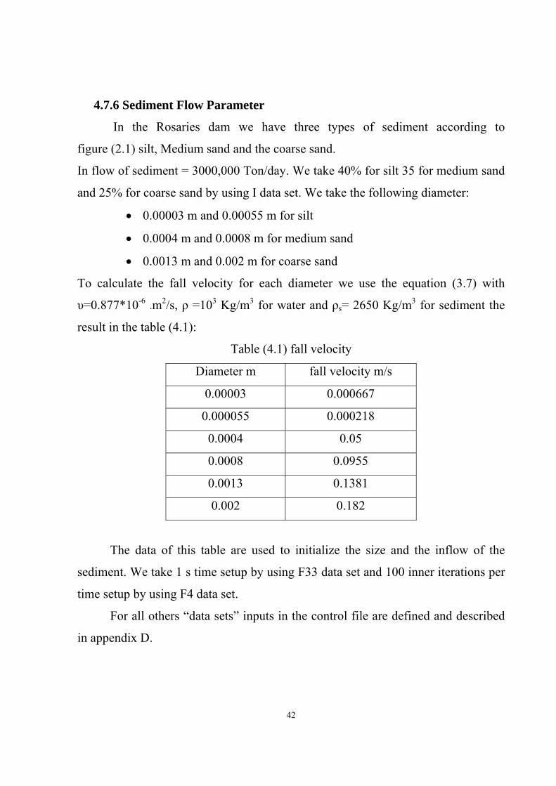
4.7.6 Sediment Flow Parameter

In the Rosaries dam we have three types of sediment according to

figure (2.1) silt, Medium sand and the coarse sand.

In flow of sediment = 3000,000 Ton/day. We take 40% for silt 35 for medium sand

and 25% for coarse sand by using I data set. We take the following diameter:

• 0.00003 m and 0.00055 m for silt

• 0.0004 m and 0.0008 m for medium sand

• 0.0013 m and 0.002 m for coarse sand

To calculate the fall velocity for each diameter we use the equation (3.7) with

υ=0.877*10-6 .m2/s, ρ =103 Kg/m3 for water and ρs= 2650 Kg/m3 for sediment the

result in the table (4.1):

Table (4.1) fall velocity

Diameter m fall velocity m/s

0.00003 0.000667

0.000055 0.000218

0.0004 0.05

0.0008 0.0955

0.0013 0.1381

0.002 0.182

The data of this table are used to initialize the size and the inflow of the

sediment. We take 1 s time setup by using F33 data set and 100 inner iterations per

time setup by using F4 data set.

For all others “data sets” inputs in the control file are defined and described

in appendix D.

43

CHAPTER - FIVE

RESULT & DISCUSSION

This chapter described the result and discussion of the SSIIM program

according to the input data in chapter four and control file in appendix (D).

5.1 The Result:

After the definition of all parameters of the problem (in the control file or

other). The solution of the problem takes about three days according to the

available used hardware (2 GHz ram and 1 processor of 3 GHz).

The convergence occurs for precision of 10-4 for all residuals (u, v, w, p, k,

and ε) this value of 10-4 is hard coded in the program. [9]

The program output data consists of many variables like velocity vectors,

sediment concentration, pressure, and turbulence kinetic energy…etc. The focus of

the analysis is in velocity vector and sediment concentration. The result shows in

the figures illustrate the velocity vectors and the sediment concentration from the

plane view (x-y plan), cross section (x-z), and longitudinal profile (y-z). This result

illustrate as velocity vectors and contour map of the sediment concentration .The

result in details and the coordinates of the geometry are given in result, conres,

boogie, and koordina files in appendix E, Appendix F, appendix G and appendix H

respectively.

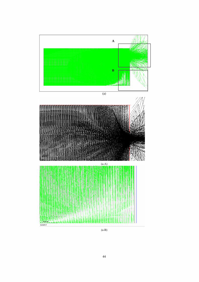
5.1.1 The Velocity Vector

The velocity vector in three dimensions is shown in figure (5.1). Figure 5.1-a

is the plane section, and figures (5.1-a-A) and (5.1-a-B) show the zooming areas A

and B. they illustrate the existence of vortices by the two sides of the gates

44

(a)

(a-A)

(a-B)

A

B

45

(b)

(c) Figure (5.1) illustrate the velocity in three dimensions

(a. plane b. longitudinal c. cross sectional)

5.1.2 Sediment Concentration:

How to read sediment concentration contours?

m.

The values of the different lines are given on the colored scale. The text at

the lower part of the figure gives the values of the maximum and minimum values,

46

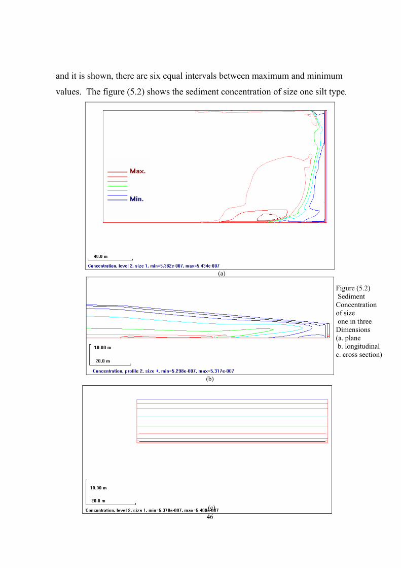
and it is shown, there are six equal intervals between maximum and minimum

values. The figure (5.2) shows the sediment concentration of size one silt type.

(a)

(b)

(c) `

Figure (5.2) Sediment Concentration of size one in three Dimensions (a. plane b. longitudinal c. cross section)

(c)

47

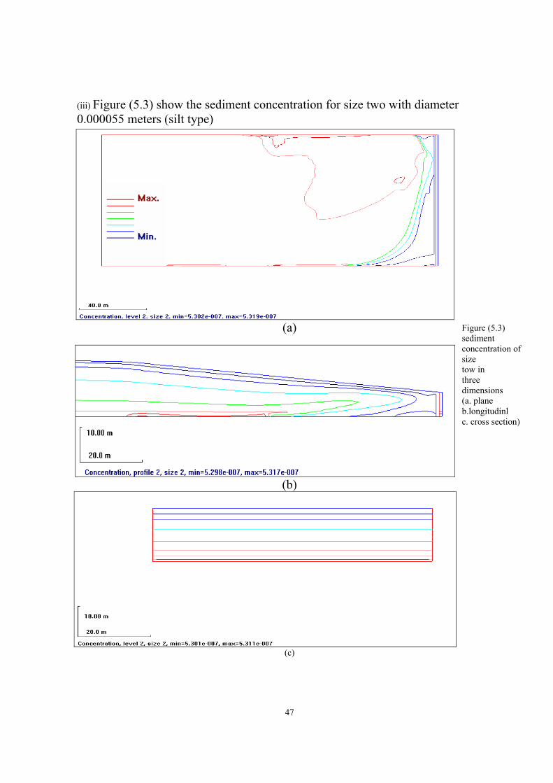
(iii) Figure (5.3) show the sediment concentration for size two with diameter 0.000055 meters (silt type)

(a)

(b)

(c)

Figure (5.3) sediment concentration of size tow in three dimensions (a. plane b.longitudinl c. cross section)

48

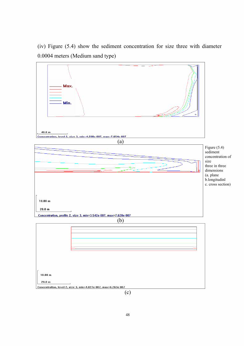
(iv) Figure (5.4) show the sediment concentration for size three with diameter

0.0004 meters (Medium sand type)

(a)

(b)

(c)

Figure (5.4) sediment concentration of size three in three dimensions (a. plane b.longitudinl c. cross section)

49

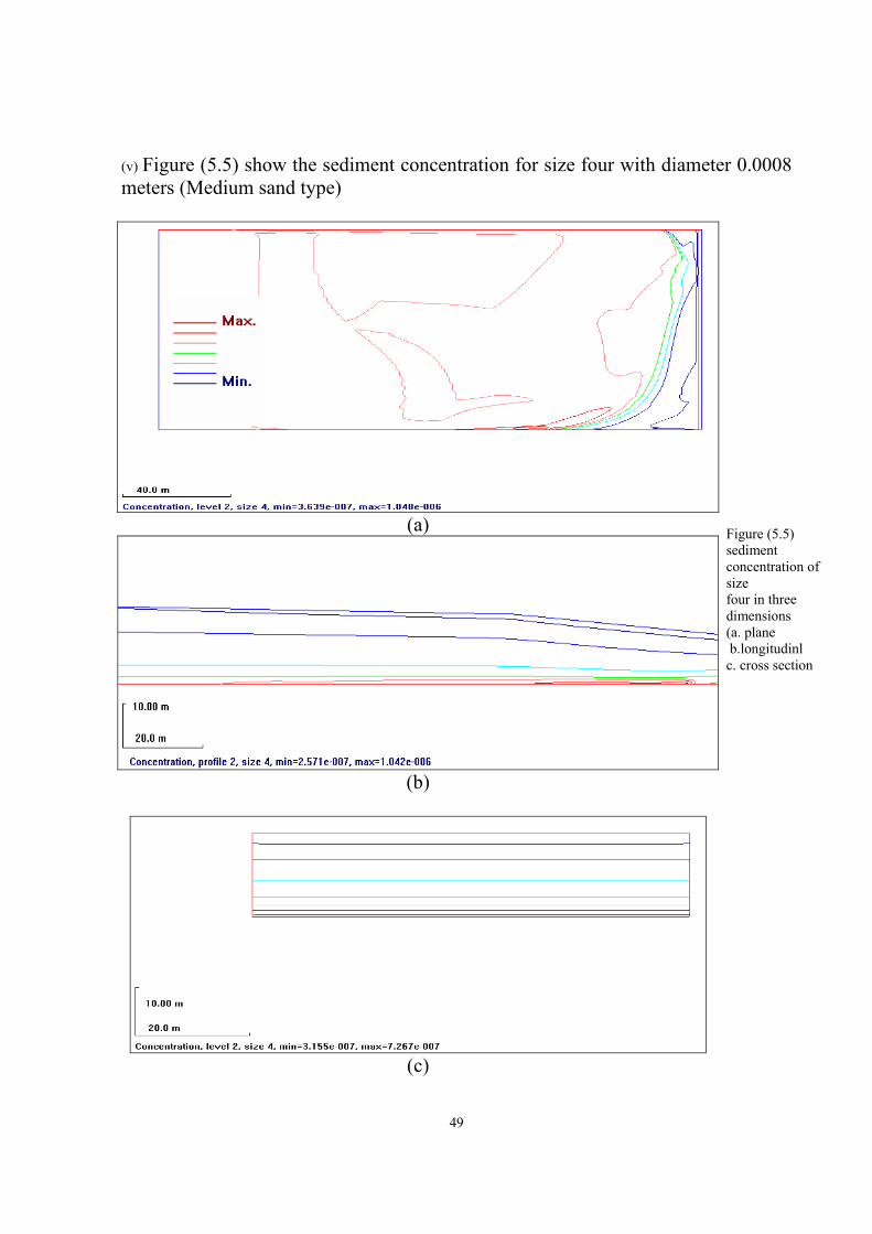
(v) Figure (5.5) show the sediment concentration for size four with diameter 0.0008 meters (Medium sand type)

(a)

(b)

(c)

Figure (5.5) sediment concentration of size four in three dimensions (a. plane b.longitudinl c. cross section

50

(vi)Figure (5.6) show the sediment concentration for size five with diameter 0.0013

meters (coarse sand type).

(a)

(b)

(c)

Figure (5.6) sediment concentration of size five in three dimensions (a. plane b.longitudinl c. cross section)

51

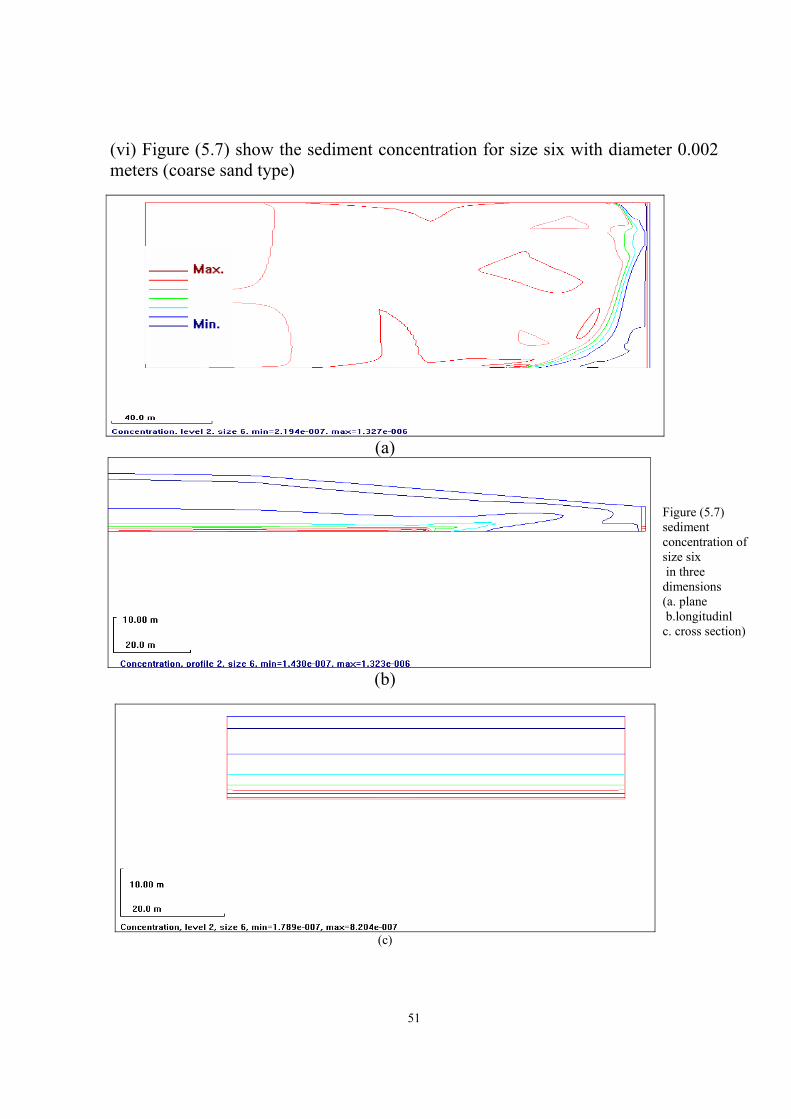
(vi) Figure (5.7) show the sediment concentration for size six with diameter 0.002 meters (coarse sand type)

(a)

(b)

(c)

Figure (5.7) sediment concentration of size six in three dimensions (a. plane b.longitudinl c. cross section)

52

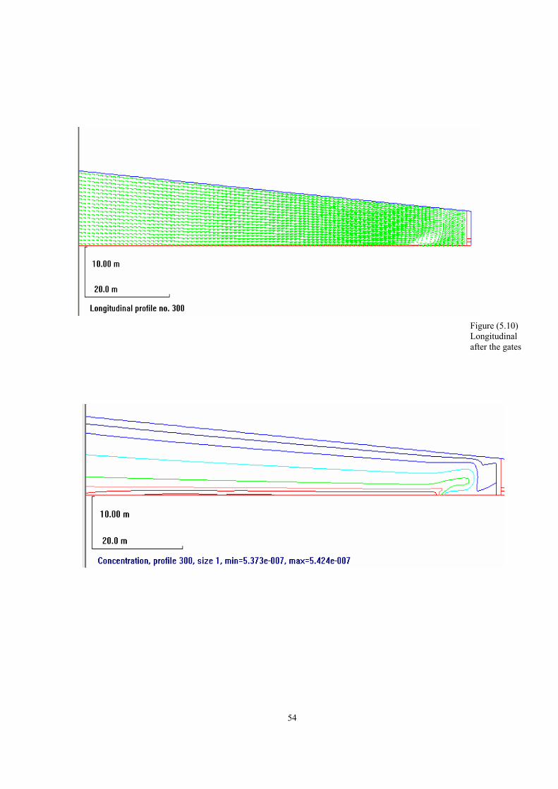
The next figures (5.8 - 5.9 - 5.10) will show the contour of sediment concentration

and velocity vectors taken at different longitudinal sections for one size of sediment

(size 1). These figures illustrate and confirm the relation between the vortices

formation and the sediment concentration, 1 section at the gates show in Fig (5.8),

3 sections before show in Fig (5.9), and 1 section after the gates show in Fig (5.10)

Figure (5.8) longitudinal profile at the gates

53

Figure (5.9) longitudinal profile before the gates at (J= 2, J= 15 and J= 100)

54

Figure (5.10) Longitudinal after the gates

55

5.2 Discussion

Generally, it is observed that at the gates, at the lower part of the dam and the

out block region, affect on the velocity vectors figure (5.1), it can be also observed

the reverse flow of water and vortices formation shows in figures (5.8, 5.9, and

5.10). The sedimentation is obviously observed and that the largest concentration of

all types of sediments corresponds to the vortices area compared with longitudinal

profile of all available types of sedimentation. And these observations are

confirmed on the figures where different longitudinal sections are taken for one

type of sediment All the plan views (5.1) illustrate that the concentration of sedimentation is

located on the sides of reservoir and this leads consequently to the formation of

islands. Comparing these different sediments concentration results with the actual

real topology of the lake, It is found that the islands are situated on the same sides

as the results obtained. Cross section views show that the concentration of sedimentation decreases

as we go downstream at the turbines gates

56

CHAPTER SIX

CONCLUSION & RECOMMENDATION 6.1 CONCLUSION: The results obtained in the previous chapter for sediments confirm clearly the

utility of the CFD for designing, predicting the motion of fluids.

The sediments concentrations obtained and shown in the figures of last chapter

illustrate that each type of sediment concentration location is different according to

its diameter.

The SSIIM program is so useful for the sediment transportation phenomenon on

open channel flow, it has more functions that are not used in this study, like the

export of results to another post-processing software helping and giving more

powerful simulations (i.e. animation of sediment movement with time)

The CFD results illustrate that the coincidence the sediments deposit with the

vortices formation in the dam

The CFD can be used for presenting and finding less costly solutions to the

sediments in the lake of Rosaries dam

57

6.2 RECOMMENDATION:

Our recommendation includes the following:

• Realising a small dam prototype model to validate the result that obtained

and to re-produce out of the open channel sedimentation.

• Carrying out the study with others packages so as to complete the

comparison between results obtained by and that by the SSIIM1 program.

• Increasing the accuracy by increasing the number of inner iterations per time

step to give more accurate results for the calculations of water and

sedimentation. To realise this, a more developed computer (RAM and

processor) will be needed so as to results can be completed in suitable time.

• To perform the study case while the seven gates of the turbines and the seven

gates of the spillway are opened and to know the effect of this on the

concentration of the sedimentation.

• To carry the program in case all gates (turbine, spill way, and deep sluices)

are open to study the changes that will take place of sedimentation and the

direction of flow.

• To reproduce the actual lake topology and re-calculate all the sediment

concentration. This production, can be done from an aerial satellite image of

the Dam

• To suggest a solution to stop sedimentation during autumn and to carry out

the suggest solution through the program to fined out its usefulness and this

will reduce the expense.

• To use the calculated efficiency of trap (the most accurate location for

dredging and to know the exact quantities of sediments) after the summer

season.

58

REFERENCES

Ref:

1. Nils Reidar B. Olsen, Computational Fluid Dynamics in Hydraulic and

Sedimentation Engineering, 2nd. revision, 16. June 1999.

2. Nils Reidar B. Olsen, CFD Algorithms for Hydraulic Engineering, 18. December

2000

3. Nils Reidar B. Olsen, CFD modelling for hydraulic structures, Preliminary 1st

edition, 8. May 2001

4. H. K. VERSTEEG and W. MALALASEKERA, An introduction to

computational fluid dynamics the finite volume method, Longman Group Ltd 1995

5. Rosaries dam maual, misistry of irreigation and hydro electric power, rebublic

of the sudan, italy-E Sormani. Milan

6. Messrs. Keohane an Quinn, report on operating and maintenance of Rosaries

hydro power station for public eletricty and water corporation sudan,1980

7. Rosaries operation manual

8. Rog´erio Campos, Three-Dimensional Reservoir Sedimentation Model,

Newcastle-upon-Tyne, December 2001

9. NILS REIDAR B. OLSEN, A Three-Dimensional Numerical Model For

Simulation Of Sediment Movements In Water Intakes With Multiblock Option,

User's Manual,2006 Web: 1. http://www.ntnu.no/~nilsol/beta

2. http://www.ntnu.no/~nilsol/ssiimwin

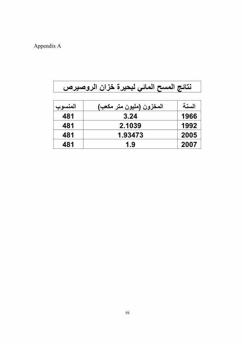
59

Appendix A

نتائج المسح المائي لبحيرة خزان الروصيرص

السنة )مليون متر مكعب(المخزون المنسوب481 3.24 1966 481 2.1039 1992 481 1.93473 2005 481 1.9 2007

60

Appendix B

POWER PLANTEQUIPMENT DEPERICIATION COST CALCULATED BY EURO TRBINE NORMAL OPERATION LIFE DEPRECIATION PART COST DAMAGE PART LIFE LIFE DESTRICTION % EURO COST INTAKE SCREEN 30 U\S MENT- GATE 50 20 30 0.6 150000 90000 INTAKE CONTROL GATE 50 20 3 0.6 256500 153900 D\S MENT- GATE 50 20 30 0.6 120000 72000 THE PENSTOCK 50 40 10 0.2 99128 19826 SPIRAL CASE 50 40 10 0.2 2450 490 STAY VANES 50 35 15 0.3 1500000 450000 GUIDE VANES 50 20 30 0.6 1243333 746000 RUNNER BLADES 50 15 35 0.7 1678725 1175107 TURBINE HUB 50 20 30 0.6 16760 10056 RUNNER BLADES CHAMBER WALL 50 40 10 0.2 9450 1890 DRAFT TUBE 50 45 5 0.1 49067 4407 THE SHAFT SEAL 10 2 8 0.8 53545 42836 TURBINE SHAFT 50 48 2 0.04 40976 1639 TURBINE GUID BEARING 20 10 10 0.5 46928 23464 P.I.PS FOR SHAFT SEALING 5 3 2 0.4 4538 1815 LKG WATER PUMPS 5 3 2 0.4 2269 908 DE-WATERING PUMPS 10 8 2 0.2 4538 908 WATER VAVES FOR COOLING 10 6 4 0.4 350 140 WATER VAVES TO DE-WATERING 25 20 5 0.2 550 110 WATER PIPES 50 40 10 0.2 12650 2530 WATER FILTERS 10 8 2 0.2 685 137 SYCLONES 25 20 5 0.2 4239 848 THRUST BRG COOLER 25 10 15 0.6 7000 4200 TURBINE BRG COOLER 10 8 2 0.2 6500 1300 GOVERNOR OIL COOLER 15 10 5 0.3 2000 667 GENERATOR AIR COOLER 10 6 4 0.4 8000 5980 WATER FLOW GUAGE 5 2 3 0.6 250 150 WATER PRESURE GUAGE 5 2 3 0.6 250 150

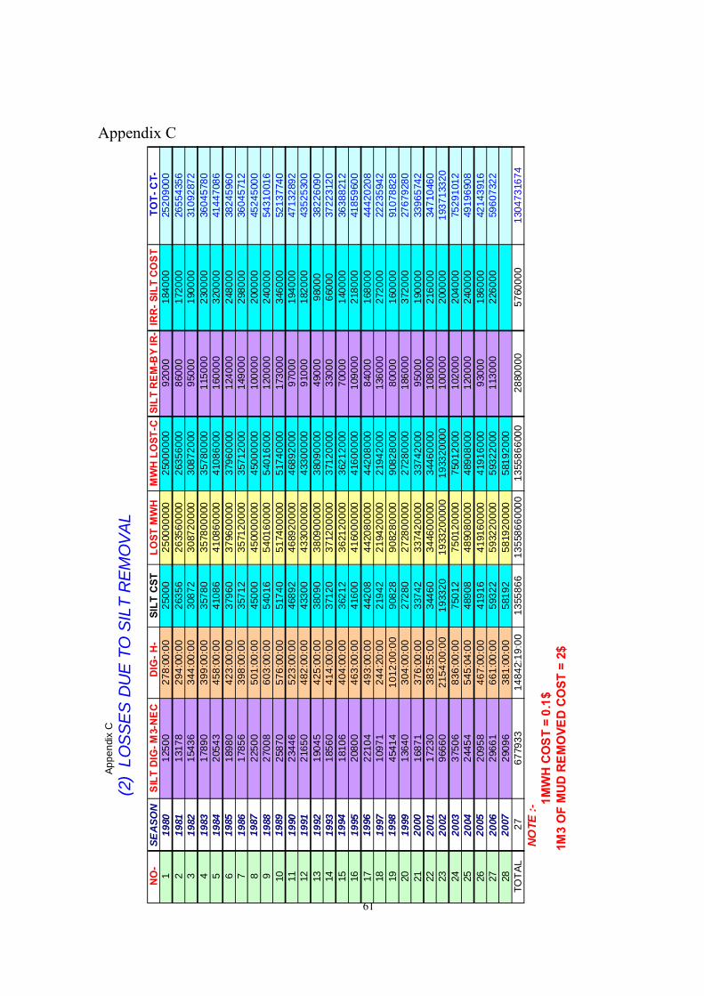
61

Ap

pend

ix C

(2

) LO

SSES

DU

E TO

SIL

T R

EMO

VAL

NO

-SE

ASO

NS

ILT

DIG

- M3-

NE

C D

IG- H

-SI

LT C

STLO

ST M

WH

MW

H L

OST

-CSI

LT R

EM

-BY

IR-

IRR

- SIL

T C

OS

T T

OT-

CT-

119

8012

500

278:

00:0

025

000

2500

0000

025

0000

0092

000

1840

0025

2090

002

1981

1317

829

4:00

:00

2635

626

3560

000

2635

6000

8600

017

2000

2655

4356

319

8215

436

344:

00:0

030

872

3087

2000

030

8720

0095

000

1900

0031

0928

724

1983

1789

039

9:00

:00

3578

035

7800

000

3578

0000

1150

0023

0000

3604

5780

519

8420

543

458:

00:0

041

086

4108

6000

041

0860

0016

0000

3200

0041

4470

866

1985

1898

042

3:00

:00

3796

037

9600

000

3796

0000

1240

0024

8000

3824

5960

719

8617

856

398:

00:0

035

712

3571

2000

035

7120

0014

9000

2980

0036

0457

128

1987

2250

050

1:00

:00

4500

045

0000

000

4500

0000

1000

0020

0000

4524

5000

919

8827

008

603:

00:0

054

016

5401

6000

054

0160

0012

0000

2400

0054

3100

1610

1989

2587

057

6:00

:00

5174

051

7400

000

5174

0000

1730

0034

6000

5213

7740

1119

9023

446

523:

00:0

046

892

4689

2000

046

8920

0097

000

1940

0047

1328

9212

1991

2165

048

2:00

:00

4330

043

3000

000

4330

0000

9100

018

2000

4352

5300

1319

9219

045

425:

00:0

038

090

3809

0000

038

0900

0049

000

9800

038

2260

9014

1993

1856

041

4:00

:00

3712

037

1200

000

3712

0000

3300

066

000

3722

3120

1519

9418

106

404:

00:0

036

212

3621

2000

036

2120

0070

000

1400

0036

3882

1216

1995

2080

046

3:00

:00

4160

041

6000

000

4160

0000

1090

0021

8000

4185

9600

1719

9622

104

493:

00:0

044

208

4420

8000

044

2080

0084

000

1680

0044

4202

0818

1997

1097

124

4:20

:00

2194

221

9420

000

2194

2000

1360

0027

2000

2223

5942

1919

9845

414

1012

:00:

0090

828

9082

8000

090

8280

0080

000

1600

0091

0788

2820

1999

1364

030

4:00

:00

2728

027

2800

000

2728

0000

1860

0037

2000

2767

9280

2120

0016

871

376:

00:0

033

742

3374

2000

033

7420

0095

000

1900

0033

9657

4222

2001

1723

038

3:55

:00

3446

034

4600

000

3446

0000

1080

0021

6000

3471

0460

2320

0296

660

2154

:00:

0019

3320

1933

2000

0019

3320

000

1000

0020

0000

1937

1332

024

2003

3750

683

6:00

:00

7501

275

0120

000

7501

2000

1020

0020

4000

7529

1012

2520

0424

454

545:

04:0

048

908

4890

8000

048

9080

0012

0000

2400

0049

1969

0826

2005

2095

846

7:00

:00

4191

641

9160

000

4191

6000

9300

018

6000

4214

3916

2720

0629

661

661:

00:0

059

322

5932

2000

059

3220

0011

3000

2260

0059

6073

2228

2007

2909

638

1:00

:00

5819

258

1920

000

5819

2000

TOTA

L27

6779

3314

842:

19:0

013

5586

613

5586

6000

013

5586

6000

2880

000

5760

000

1304

7316

74N

OTE

:-1M

WH

CO

ST

= 0.

1$1M

3 O

F M

UD

RE

MO

VED

CO

ST =

2$

Appendix C

62

Appendix D T rosiers dam

F 2 IS

F 4 0.8 50 0.00001

F 33 1 20

F 37 1

G 1 201 300 21 6 grid and array sizes

G 3 0 5 10 15 20 25 30 35 40 45 50 55 60 65 70 75 80 85 90 95 100 vertical grid distribution

G 7 0 1 2 300 2 21 0 0 70000.0 1 0 0

G 7 1 -1 221 222 4 5 0 0 10000.0 1 0 0

G 7 1 -1 225 226 4 5 0 0 10000.0 1 0 0

G 7 1 -1 229 230 4 5 0 0 10000.0 1 0 0

G 7 1 -1 233 234 4 5 0 0 10000.0 1 0 0

G 7 1 -1 237 238 4 5 0 0 10000.0 1 0 0

G 7 1 -1 241 242 4 5 0 0 10000.0 1 0 0

G 7 1 -1 245 246 4 5 0 0 10000.0 1 0 0

G 13 3 201 201 2 300 6 21

G 13 3 201 201 2 300 2 3

G 13 3 201 201 2 220 4 5

G 13 3 201 201 223 224 4 5

G 13 3 201 201 227 228 4 5

G 13 3 201 201 231 232 4 5

G 13 3 201 201 235 236 4 5

G 13 3 201 201 239 240 4 5

G 13 3 201 201 243 244 4 5

G 13 3 201 201 247 300 4 5

W 1 50.000000 70000.000000 6.800000

W 2 3 1 100 201

K 1 300 60000

K 2 0 1

63

k 5 1 1 1 1 1 1

k 6 1 1 1 0 0 0

S 1 0.00003 0.000667

S 2 0.000055 .000218

S 3 0.0004 0.05

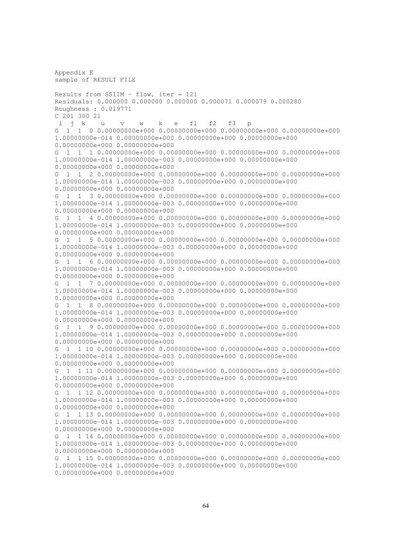
64

Appendix E sample of RESULT FILE Results from SSIIM - flow, iter = 121 Residuals: 0.000000 0.000000 0.000000 0.000071 0.000079 0.000280 Roughness : 0.019771 C 201 300 21 i j k u v w k e f1 f2 f3 p G 1 1 0 0.00000000e+000 0.00000000e+000 0.00000000e+000 0.00000000e+000 1.00000000e-014 0.00000000e+000 0.00000000e+000 0.00000000e+000 0.00000000e+000 0.00000000e+000 G 1 1 1 0.00000000e+000 0.00000000e+000 0.00000000e+000 0.00000000e+000 1.00000000e-014 1.00000000e-003 0.00000000e+000 0.00000000e+000 0.00000000e+000 0.00000000e+000 G 1 1 2 0.00000000e+000 0.00000000e+000 0.00000000e+000 0.00000000e+000 1.00000000e-014 1.00000000e-003 0.00000000e+000 0.00000000e+000 0.00000000e+000 0.00000000e+000 G 1 1 3 0.00000000e+000 0.00000000e+000 0.00000000e+000 0.00000000e+000 1.00000000e-014 1.00000000e-003 0.00000000e+000 0.00000000e+000 0.00000000e+000 0.00000000e+000 G 1 1 4 0.00000000e+000 0.00000000e+000 0.00000000e+000 0.00000000e+000 1.00000000e-014 1.00000000e-003 0.00000000e+000 0.00000000e+000 0.00000000e+000 0.00000000e+000 G 1 1 5 0.00000000e+000 0.00000000e+000 0.00000000e+000 0.00000000e+000 1.00000000e-014 1.00000000e-003 0.00000000e+000 0.00000000e+000 0.00000000e+000 0.00000000e+000 G 1 1 6 0.00000000e+000 0.00000000e+000 0.00000000e+000 0.00000000e+000 1.00000000e-014 1.00000000e-003 0.00000000e+000 0.00000000e+000 0.00000000e+000 0.00000000e+000 G 1 1 7 0.00000000e+000 0.00000000e+000 0.00000000e+000 0.00000000e+000 1.00000000e-014 1.00000000e-003 0.00000000e+000 0.00000000e+000 0.00000000e+000 0.00000000e+000 G 1 1 8 0.00000000e+000 0.00000000e+000 0.00000000e+000 0.00000000e+000 1.00000000e-014 1.00000000e-003 0.00000000e+000 0.00000000e+000 0.00000000e+000 0.00000000e+000 G 1 1 9 0.00000000e+000 0.00000000e+000 0.00000000e+000 0.00000000e+000 1.00000000e-014 1.00000000e-003 0.00000000e+000 0.00000000e+000 0.00000000e+000 0.00000000e+000 G 1 1 10 0.00000000e+000 0.00000000e+000 0.00000000e+000 0.00000000e+000 1.00000000e-014 1.00000000e-003 0.00000000e+000 0.00000000e+000 0.00000000e+000 0.00000000e+000 G 1 1 11 0.00000000e+000 0.00000000e+000 0.00000000e+000 0.00000000e+000 1.00000000e-014 1.00000000e-003 0.00000000e+000 0.00000000e+000 0.00000000e+000 0.00000000e+000 G 1 1 12 0.00000000e+000 0.00000000e+000 0.00000000e+000 0.00000000e+000 1.00000000e-014 1.00000000e-003 0.00000000e+000 0.00000000e+000 0.00000000e+000 0.00000000e+000 G 1 1 13 0.00000000e+000 0.00000000e+000 0.00000000e+000 0.00000000e+000 1.00000000e-014 1.00000000e-003 0.00000000e+000 0.00000000e+000 0.00000000e+000 0.00000000e+000 G 1 1 14 0.00000000e+000 0.00000000e+000 0.00000000e+000 0.00000000e+000 1.00000000e-014 1.00000000e-003 0.00000000e+000 0.00000000e+000 0.00000000e+000 0.00000000e+000 G 1 1 15 0.00000000e+000 0.00000000e+000 0.00000000e+000 0.00000000e+000 1.00000000e-014 1.00000000e-003 0.00000000e+000 0.00000000e+000 0.00000000e+000 0.00000000e+000

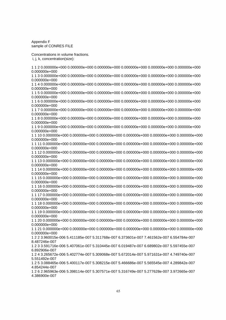
65

Appendix F sample of CONRES FILE Concentrations in volume fractions. i, j, k, concentration(size): 1 1 2 0.000000e+000 0.000000e+000 0.000000e+000 0.000000e+000 0.000000e+000 0.000000e+000 0.000000e+000 1 1 3 0.000000e+000 0.000000e+000 0.000000e+000 0.000000e+000 0.000000e+000 0.000000e+000 0.000000e+000 1 1 4 0.000000e+000 0.000000e+000 0.000000e+000 0.000000e+000 0.000000e+000 0.000000e+000 0.000000e+000 1 1 5 0.000000e+000 0.000000e+000 0.000000e+000 0.000000e+000 0.000000e+000 0.000000e+000 0.000000e+000 1 1 6 0.000000e+000 0.000000e+000 0.000000e+000 0.000000e+000 0.000000e+000 0.000000e+000 0.000000e+000 1 1 7 0.000000e+000 0.000000e+000 0.000000e+000 0.000000e+000 0.000000e+000 0.000000e+000 0.000000e+000 1 1 8 0.000000e+000 0.000000e+000 0.000000e+000 0.000000e+000 0.000000e+000 0.000000e+000 0.000000e+000 1 1 9 0.000000e+000 0.000000e+000 0.000000e+000 0.000000e+000 0.000000e+000 0.000000e+000 0.000000e+000 1 1 10 0.000000e+000 0.000000e+000 0.000000e+000 0.000000e+000 0.000000e+000 0.000000e+000 0.000000e+000 1 1 11 0.000000e+000 0.000000e+000 0.000000e+000 0.000000e+000 0.000000e+000 0.000000e+000 0.000000e+000 1 1 12 0.000000e+000 0.000000e+000 0.000000e+000 0.000000e+000 0.000000e+000 0.000000e+000 0.000000e+000 1 1 13 0.000000e+000 0.000000e+000 0.000000e+000 0.000000e+000 0.000000e+000 0.000000e+000 0.000000e+000 1 1 14 0.000000e+000 0.000000e+000 0.000000e+000 0.000000e+000 0.000000e+000 0.000000e+000 0.000000e+000 1 1 15 0.000000e+000 0.000000e+000 0.000000e+000 0.000000e+000 0.000000e+000 0.000000e+000 0.000000e+000 1 1 16 0.000000e+000 0.000000e+000 0.000000e+000 0.000000e+000 0.000000e+000 0.000000e+000 0.000000e+000 1 1 17 0.000000e+000 0.000000e+000 0.000000e+000 0.000000e+000 0.000000e+000 0.000000e+000 0.000000e+000 1 1 18 0.000000e+000 0.000000e+000 0.000000e+000 0.000000e+000 0.000000e+000 0.000000e+000 0.000000e+000 1 1 19 0.000000e+000 0.000000e+000 0.000000e+000 0.000000e+000 0.000000e+000 0.000000e+000 0.000000e+000 1 1 20 0.000000e+000 0.000000e+000 0.000000e+000 0.000000e+000 0.000000e+000 0.000000e+000 0.000000e+000 1 1 21 0.000000e+000 0.000000e+000 0.000000e+000 0.000000e+000 0.000000e+000 0.000000e+000 0.000000e+000 1 2 2 3.960015e-006 5.411185e-007 5.311768e-007 6.373601e-007 7.461562e-007 6.554784e-007 8.487246e-007 1 2 3 3.591716e-006 5.407061e-007 5.310445e-007 6.019487e-007 6.689802e-007 5.597455e-007 6.892906e-007 1 2 4 3.265672e-006 5.402774e-007 5.309068e-007 5.672014e-007 5.971631e-007 4.749740e-007 5.551492e-007 1 2 5 3.088465e-006 5.400117e-007 5.308215e-007 5.466686e-007 5.565545e-007 4.289842e-007 4.854244e-007 1 2 6 2.965963e-006 5.398114e-007 5.307571e-007 5.316749e-007 5.277628e-007 3.972665e-007 4.386900e-007

66

Appendix G sample of KOORDINA FILE 1 1 0.000000 0.000000 0.0 1 2 0.000000 0.334448 0.0 1 3 0.000000 0.668896 0.0 1 4 0.000000 1.003344 0.0 1 5 0.000000 1.337793 0.0 1 6 0.000000 1.672241 0.0 1 7 0.000000 2.006689 0.0 1 8 0.000000 2.341137 0.0 1 9 0.000000 2.675585 0.0 1 10 0.000000 3.010033 0.0 1 11 0.000000 3.344482 0.0 1 12 0.000000 3.678930 0.0 1 13 0.000000 4.013378 0.0 1 14 0.000000 4.347826 0.0 1 15 0.000000 4.682274 0.0 1 16 0.000000 5.016722 0.0 1 17 0.000000 5.351171 0.0 1 18 0.000000 5.685619 0.0 1 19 0.000000 6.020067 0.0 1 20 0.000000 6.354515 0.0 1 21 0.000000 6.688963 0.0 1 22 0.000000 7.023411 0.0 1 23 0.000000 7.357860 0.0 1 24 0.000000 7.692308 0.0 1 25 0.000000 8.026756 0.0 1 26 0.000000 8.361204 0.0 1 27 0.000000 8.695652 0.0 1 28 0.000000 9.030100 0.0 1 29 0.000000 9.364548 0.0 1 30 0.000000 9.698997 0.0 1 31 0.000000 10.033445 0.0 1 32 0.000000 10.367893 0.0 1 33 0.000000 10.702341 0.0 1 34 0.000000 11.036789 0.0 1 35 0.000000 11.371237 0.0 1 36 0.000000 11.705686 0.0 1 37 0.000000 12.040134 0.0 1 38 0.000000 12.374582 0.0 1 39 0.000000 12.709030 0.0 1 40 0.000000 13.043478 0.0 1 41 0.000000 13.377926 0.0 1 42 0.000000 13.712375 0.0 1 43 0.000000 14.046823 0.0 1 44 0.000000 14.381271 0.0 1 45 0.000000 14.715719 0.0 1 46 0.000000 15.050167 0.0 1 47 0.000000 15.384615 0.0 1 48 0.000000 15.719064 0.0 1 49 0.000000 16.053512 0.0 1 50 0.000000 16.387960 0.0 1 51 0.000000 16.722408 0.0 1 52 0.000000 17.056856 0.0

67

Appendix G Sample of data in BOOGIE FILE Multi-block version of SSIIM In kread Transient inner iterations: 20 In osiio1: IONo = 8 TurbulenceModel = 0 In initial - arrays End of initial - arrays Have allocated 798.28 Mbytes In initial - velocity Loop1,iter,area,radius,velocity,waterlevel: 9 1.560713e+003 1.560713e+001 4.485130e+001 1.560713e+001 Loop1,iter,area,radius,velocity,waterlevel: 17 1.732627e+003 1.732627e+001 4.040108e+001 1.732627e+001 Waterlevel = 6.887199 meters for cross-section i = 200 Waterlevel = 6.974399 meters for cross-section i = 199 Waterlevel = 7.061598 meters for cross-section i = 198 Waterlevel = 7.148797 meters for cross-section i = 197 Waterlevel = 7.235996 meters for cross-section i = 196 Waterlevel = 7.323196 meters for cross-section i = 195 Waterlevel = 7.410395 meters for cross-section i = 194 Waterlevel = 7.497594 meters for cross-section i = 193 Waterlevel = 7.584794 meters for cross-section i = 192 Waterlevel = 7.671993 meters for cross-section i = 191 Waterlevel = 7.759192 meters for cross-section i = 190 Waterlevel = 7.846391 meters for cross-section i = 189 Waterlevel = 7.933591 meters for cross-section i = 188 Waterlevel = 8.020790 meters for cross-section i = 187 Waterlevel = 8.107989 meters for cross-section i = 186 Waterlevel = 8.195188 meters for cross-section i = 185 Waterlevel = 8.282388 meters for cross-section i = 184 Waterlevel = 8.369587 meters for cross-section i = 183 Waterlevel = 8.456786 meters for cross-section i = 182 Waterlevel = 8.543986 meters for cross-section i = 181 Waterlevel = 8.631185 meters for cross-section i = 180 Waterlevel = 8.718384 meters for cross-section i = 179 Waterlevel = 8.805583 meters for cross-section i = 178 Waterlevel = 8.892783 meters for cross-section i = 177 Waterlevel = 8.979982 meters for cross-section i = 176 Waterlevel = 9.067181 meters for cross-section i = 175 Waterlevel = 9.154381 meters for cross-section i = 174 Waterlevel = 9.241580 meters for cross-section i = 173 Waterlevel = 9.328779 meters for cross-section i = 172 Waterlevel = 9.415978 meters for cross-section i = 171 Waterlevel = 9.503178 meters for cross-section i = 170 Waterlevel = 9.590377 meters for cross-section i = 169 Waterlevel = 9.677576 meters for cross-section i = 168 Waterlevel = 9.764775 meters for cross-section i = 167 Waterlevel = 9.851975 meters for cross-section i = 166 Waterlevel = 9.939174 meters for cross-section i = 165

68