Embed Size (px)
Citation preview

arX
iv:1
710.
1040
9v2
[he
p-th
] 2
6 Ja
n 20
18KOBE-TH-17-05
On the geometry of the theory space in the ERG formalism
C. Pagani∗
Institute fur Physik (WA THEP) Johannes-Gutenberg-Universitat
Staudingerweg 7, 55099 Mainz, Germany
H. Sonoda†
Physics Department, Kobe University, Kobe 657-8501, Japan
(Dated: January 29, 2018)
Abstract
We consider the theory space as a manifold whose coordinates are given by the couplings appear-
ing in the Wilson action. We discuss how to introduce connections on this theory space. A partic-
ularly intriguing connection can be defined directly from the solution of the exact renormalization
group (ERG) equation. We advocate a geometric viewpoint that lets us define straightforwardly
physically relevant quantities invariant under the changes of a renormalization scheme.
∗ [email protected]† [email protected]
1

I. INTRODUCTION
The theory space is a key ingredient of our modern understanding of quantum and sta-
tistical field theory. On very general grounds, one may define the theory space as the set of
theories that are identified by the following common features: dimensionality, field content,
and symmetries. The renormalization group (RG) brings further qualitative and quantita-
tive information through the notion of relevant, irrelevant, and marginal directions. Indeed,
the study of the RG flow of the couplings allows us to define the continuum limit of quantum
field theories and to derive the scaling properties of the operators by studying the linearized
RG flow around a fixed point [1].
In this work we study the possibility of considering the theory space as a manifold with
geometric structures. In particular, we will show that it is possible to define connections
on the theory space. The introduction of a connection is an important step as it allows us
to study in a general way both local and global quantities defined over the theory space.
We will pay particular attention to a connection stemming directly and nonperturbatively
from the exact renormalization group (ERG) equation. By means of a connection, it is
then straightforward to construct the quantities that are invariant under the changes of
coordinates. A coordinate change can be identified as a change of schemes (choice of a
cutoff function in the ERG framework). Scheme independence is important since physical
observables such as critical exponents are scheme independent.
In different forms, a geometric viewpoint of the theory space has already been invoked
in the past. In [2], the RG flow is identified as a one-parameter group of diffeomorphism
generated by the beta functions as a vector field. A connection was also identified in the
formulation of renormalization in coordinate space by requiring covariant transformation
properties of the correlation functions [3, 4]. Apart from the linearized behavior around the
fixed point, little effort has been made to investigate seriously the information encoded in the
RG flow beyond critical exponents. More recently, however, the transformation properties
of RG flows at the second order around a fixed point have been considered in order to make
contact with the operator product expansion (OPE) [5, 6]. We will comment also on the
relation between our result and the OPE.
The paper is organized as follows. In Sec. II we introduce the theory space as a manifold
and explain its basic features. In Sec. III we consider the ERG equation and show that
2

its solution implies the existence of a connection and define its curvature. In Sec. IV we
consider a covariant expansion of the RG flow and comment on its possible applications. In
Sec. V we generalize our consideration to the full (infinite-dimensional) theory space. We
summarize our findings in Sec. VI.
II. THE THEORY SPACE AS A MANIFOLD
In the Wilsonian renormalization program, one is instructed to write in the action all
possible terms compatible with the symmetries and the field content of the theory. Gener-
ally, this implies that one has to consider infinitely many terms in the Wilson action, and
consequently introduce infinitely many couplings. Therefore, the theory space is, generally
speaking, infinite-dimensional. However, if we consider only theories that are defined in
the continuum limit, the actual dimension of the space spanned by the theory is N , the
number of relevant directions associated to the fixed point. In this work we will mainly
consider this latter setting and take a field theory whose continuum limit is well defined.
This permits us to work with a finite-dimensional manifold. Some considerations regarding
the infinite-dimensional theory space will be given in Sec. V.
Let gi (i = 1, · · · , N) be the N coupling constants parametrizing the theory.1 We view the
couplings gi as coordinates of the theory space and view the latter as a manifold. A change of
scheme, or cutoff function in the ERG case, results in a possibly very complicated redefinition
of the couplings: g′i = g′i (g). We view such a redefinition as a change of coordinates on the
theory space. Note that schemes like minimal subtraction are not included straightforwardly
in the functional RG equations, although it is known how to retain the former’s quantities
from the latter, see [7] and references therein. Physical quantities should not depend on
the RG scheme employed. Hence, in the ERG framework, physical quantities should be
independent from the chosen cutoff function, or, equivalently, from the specific coordinates
employed.
The RG flow is expressed by the beta functions, which constitute a vector field over the
theory space. More precisely, a RG trajectory is described by the beta functions
βi =dgi
dt(i = 1, · · · , N) (1)
1 Throughout this work the couplings gi are taken to be dimensionless as all dimensionful quantities have
been rescaled in units of the cutoff.
3

that enjoy the transformation properties of a vector under a coordinate change. (We define
the “RG-time” t by t ≡ − log Λµ, where Λ is the cutoff scale introduced in Sec. III.)
As we already said, physical quantities must be independent of the RG scheme used
to compute them. Translated into a geometric language, this means that physical quanti-
ties must be invariant under any change of coordinates. An example of such a coordinate
invariant quantity is the critical exponents. Let us consider
∂βi
∂gj=
∂
∂gj
N∑
k=1
(
∂gi
∂g′kβ ′k
)
=
N∑
k,l=1
(
∂g′l
∂gj∂2gi
∂g′l∂g′kβ ′k +
∂g′l
∂gj∂β ′k
∂g′l∂gi
∂g′k
)
. (2)
It is clear that at a fixed point g∗ the first term in (2) vanishes. The critical exponents are
defined as the eigenvalues of the matrix ∂jβi at the fixed point. Since the eigenvalues are
independent of the basis used to compute them, we see that the matrices ∂jβi and ∂′
jβ′i
possess the same spectrum, and hence yield the same critical exponents. For later purposes,
let us denote the eigendecomposition of the linearized RG flow at the fixed point as follows:
∂βi
∂gj
∣
∣
∣
g=g∗=
N∑
m,n=1
AimY
mn
(
A−1)n
j, (3)
where Y is the eigenvalue matrix, and A is the eigenvector matrix. It is straightforward to
check that Aij =
∑N
k=1∂gi
∂g′kA′k
j .
We note that the coordinate independence of the critical exponents relies crucially on
the vanishing of the inhomogeneous term in (2) at the fixed point, so that the matrix of the
linearized RG flow transforms covariantly under a coordinate transformation at the fixed
point. It is clear, however, that no such simplification occurs when taking further derivatives
of the beta function. To obviate such difficulties, instead of employing partial derivatives, it
is natural to employ covariant derivatives that allow us to write down covariant quantities
directly. It is the purpose of this work to show that such a geometric structure, namely a
connection on the tangent space, can naturally be introduced from the ERG flow equation.
III. A CONNECTION FROM THE ERGE
Let S[φ] be a bare action with an ultraviolet (UV) cutoff incorporated. Following [8], we
introduce WΛ[J ], the generating functional of connected Green functions with an infrared
4

(IR) cutoff Λ, by
eWΛ[J ] ≡
∫
Dφ e−S[φ]−∆SΛ+∫ddx Jφ , (4)
where
∆SΛ =1
2
∫
ddxφ(x)RΛ
(
−∂2)
φ(x)
is an IR regulator. The kernel RΛ (−∂2) suppresses the integration over the modes with
momenta lower than the scale Λ in (4). If we denote the Fourier transform of RΛ by the
same symbol RΛ(p), it approaches a positive constant of order Λ2 as p2 → 0, and vanishes
at large momentum.
The Λ-dependence of WΛ, derived in [8], is given by
− Λ∂WΛ[J ]
∂Λ=
∫
p
Λ∂RΛ(p)
∂Λ
1
2
{
δWΛ[J ]
δJ(−p)
δWΛ[J ]
δJ(p)+
δ2WΛ[J ]
δJ(−p)δJ(p)
}
. (5)
Here, we wish to consider instead a generalized equation with a positive anomalous dimension
η/2 for the scalar field [9]:
−Λ∂WΛ[J ]
∂Λ=
η
2
∫
p
J(p)δWΛ[J ]
δJ(p)
+
∫
p
(
Λ∂
∂Λ− η
)
RΛ(p) ·1
2
{
δWΛ[J ]
δJ(−p)
δWΛ[J ]
δJ(p)+
δ2WΛ[J ]
δJ(−p)δJ(p)
}
. (6)
In the dimensionful convention adopted here, the N parameters of the theory, say Gi (i =
1, · · · , N), do not run as Λ changes. To obtain the running parameters of Sec. II, we
introduce gi(t;G) (i = 1, · · · , N) as the solution of
∂
∂tgi(t;G) = βi (g) , (7)
satisfying the initial condition
gi(0;G) = Gi . (8)
We then define
gi ≡ gi(
− lnΛ
µ;G
)
, (9)
where µ is a reference scale, such that
limΛ→∞
gi = gi∗ , (10)
where g∗ denotes the fixed point. These g’s are the parameters discussed in Sec. II, and they
parametrize the theory in the dimensionless convention.
5

To switch to the dimensionless convention we divide all physical quantities by appropriate
powers of Λ to make them dimensionless. We define
J(p) ≡ Λd−2
2 J(pΛ) (11)
which is a dimensionless field with dimensionless momentum. We then define
W (g)[J ] ≡ WΛ(G)[J ] , (12)
where g’s are related to G’s via (9). All the Λ-dependence of the original functional has been
incorporated into g’s and J . We wish to emphasize that we consider only theories in the
continuum limit. The Wilson action and the functional W have an infinite number of terms,
but they are related so that these functionals depend only on a finite number of couplings.
In Appendix C, we give an explicit but perturbative construction of a continuum limit. The
continuum limit in the ERG framework has been discussed in detail in Ref. [10].
For fixed G’s, we have
− Λ∂
∂Λgi∣
∣
∣
G= βi(g) , (13)
and for fixed J , (11) gives
− Λ∂
∂ΛJ(p)
∣
∣
∣
J=
(
d− 2
2+ p · ∂
)
J(p) . (14)
Thus, we obtain
− Λ∂
∂ΛWΛ(G)[J ] =
N∑
i=1
βi(g)∂
∂giW (g)[J ] +
∫
p
(
d− 2
2+ p · ∂
)
J(p)δ
δJ(p)W (g)[J ] . (15)
Hence, (6) implies that W (g)[J ] obeys the ERG differential equation
N∑
i=1
βi(g)∂
∂giW (g)[J ] =
∫
p
(
d− 2 + η
2+ p · ∂
)
J(p) ·δW (g)[J ]
δJ(p)
+
∫
p
(2− η − p · ∂)R(p)1
2
{
δW (g)
δJ(p)
δW (g)
δJ(−p)+
δ2W (g)
δJ(p)δJ(−p)
}
, (16)
where R(p) is related to RΛ(p) of Sec. II by
RΛ(p) = Λ2R(p/Λ) . (17)
From now on we work only in the dimensionless convention, and we omit the bar above J .
6
For our purposes, it is useful to think of W as a function of the couplings, W = W (g),
which is a scalar on the theory space, W (g) = W ′ (g′). By taking a derivative with respect
to gi, we obtain a zero momentum operator
Oi ≡∂W (g)
∂gi(18)
that has covariant transformation properties:
Oi =∂g′j
∂giO′
j , (19)
where we have adopted the Einstein convention for repeated indices.
In full analogy we can define the products of the operators Oi as follows
[Oi1 · · ·Oin ] ≡ e−W (g) ∂
∂gi1· · ·
∂
∂gineW (g) . (20)
For the case of [Oi1Oi2 ] we have
[Oi1Oi2 ] ≡∂W
∂gi1∂W
∂gi2+
∂2W
∂gi1∂gi2. (21)
Clearly [Oi1Oi2 ] is not a covariant quantity. This is because the “connected term”
Pij ≡∂2W
∂gi∂gj(22)
is not covariant. Furthermore, [Oi1Oi2 ] is related to the product of two (zero momentum)
operators, and Pij is related to the short distance singularities of this product. Thus, one
expects Pij to be related to the OPE’s singularities. The precise relation is hindered by the
the fact that we are considering zero momentum operators (i.e. operators integrated over
space). (A detailed discussion regarding [Oi1Oi2 ] and Pij in the general case of momentum-
dependent operators can be found in [11].)
Now we consider the flow equation for the operators Oi and their products. The flow of
the operator Oi can be directly obtained from (16) by taking a derivative with respect to gi:
∂βk
∂giOk +
(
β ·∂
∂g
)
Oi = DOi , (23)
(please recall the Einstein convention for the repeated k) where we define
D ≡
∫
p
[
(
d− 2 + η
2+ p · ∂p
)
J(p) ·δ
δJ(p)
+ (2− η − p · ∂)R(p) ·
{
δW (g)
δJ(−p)
δ
δJ(p)+
1
2
δ2
δJ(p)δJ(−p)
}
]
. (24)
7
In deriving (23) we assume that the anomalous dimension η is independent of g’s. This is
actually true only near the fixed point. The extension to a g-dependent anomalous dimension
is given in Appendix A.
By taking a further derivative of the flow equation (16) with respect to gj, we deduce the
flow equation for Pij. This can be written as:
∂2βk
∂gi∂gjOk +
∂βk
∂gjPki +
∂βk
∂giPkj +
(
βk ∂
∂gk−D
)
Pij =
∫
p
(
(2− η)R(
p2)
− p · ∂pR(
p2)) δOi
δJ (p)
δOj
δJ (−p). (25)
It is interesting to observe that the RHS of (25) is covariant since it is determined by the
product of the covariant operators Oi and Oj . It follows also that the LHS of (25) must be
covariant, too.
In order to investigate the covariance of the LHS of (25), let us consider the transformation
properties of Pij:
P ′ij =
∂gk
∂g′i∂gl
∂g′jPkl +
∂2gk
∂g′i∂g′jOk . (26)
Pij is not covariant. Hence, the product [OiOj ] is not covariant as was already pointed out.
Now we expand Pij in terms of a basis of composite operators:
Pij =N∑
k=1
Γ ki jOk +
∞∑
a=N+1
Γ ai jOa , (27)
where the operators Ok with k ∈ [1, N ] are the relevant operators conjugate to the couplings
gk, whereas the operators Oa with a ∈ [N + 1,∞) are irrelevant operators. By inserting the
expansion (27) into (26), we deduce the transformation properties of the terms appearing
in (27). More precisely, we find that
Γ′ikj =
∂g′k
∂gn∂gl
∂g′i∂gm
∂g′jΓ nl m +
∂g′k
∂gl∂2gl
∂g′i∂g′j, (28)
for (i, j, k) ∈ [1, N ] so that Γikj transforms as a connection in the theory space. Moreover,
we deduce that the second term in (27) transforms as a tensor:
∞∑
a=N+1
Γ′iajO
′a =
∂gk
∂g′i∂gl
∂g′j
∞∑
a=N+1
Γ ak lOa . (29)
Equation (27), together with the transformation properties (28) and (29), is one of the main
results of this section. Indeed, our findings entail that, by solving the flow equation, we can
8

determine a connection over theory space by considering the expansion of Pij in (27). Note
also that, by definition, this connection is torsionless, i.e., symmetric in the lower indices.
It is now natural to come back to Eq. (25) and consider its LHS in view of the expansion
(27) and the new connection. To do so, we also expand the RHS of (25):∫
p
(
(2− η)R(
p2)
− p · ∂pR(
p2)) δOi
δJ (p)
δOj
δJ (−p)= dkijOk + · · · , (30)
where the dots are contributions involving only irrelevant composite operators. In the fol-
lowing we focus our attention solely on the relevant operators Oi (i = 1, · · · , N).
As we have already pointed out, the RHS of (25) is covariant, and the LHS should be
also. By inserting the expansions (27) and (30) into (25), we find
[
βl ∂
∂glΓ ki j − Γ l
i j
∂βk
∂gl+
∂βl
∂gjΓ kl i +
∂βl
∂giΓ kl j +
∂2βk
∂gi∂gj
]
Ok = dkijOk , (31)
where we have kept only the terms involving relevant operators in the expansions (27) and
(30). The LHS of (31) can be rewritten in a geometric fashion and, by selecting the term
proportional to Ok, we can write
1
2(∇i∇j +∇j∇i) β
k −1
2
(
R kil j +R k
jl i
)
βl = dkij , (32)
where the covariant derivatives are defined as usual as
∇iβj ≡ ∂iβ
j + Γ ji kβ
k , (33a)
∇i∇jβk ≡ ∂i
(
∇jβk)
− Γ li j∇lβ
k + Γ ki l∇jβ
l , (33b)
and the curvature is defined by
R kil j ≡ ∂iΓ
kl j − ∂lΓ
ki j + Γ k
i mΓml j − Γ k
l mΓmi j . (34)
Equation (32) is one of the main results of this paper. It shows that the flow equation
for Pij can be written in an inspiring covariant form thanks to the connection defined by
Eq. (27). We also wish to point out that a relation very similar to our Eq. (32) was derived
in a non-ERG context in [4]. (See also [12].) More details on the derivation of Eq. (32) are
given in Appendix B.
Let us observe that we have constructed the connection Γ ki j using the generating func-
tional W . However, it can be checked that the same steps can be repeated both for the
Wilson action [1, 13] and for the effective average action (EAA) [8, 14, 15].
9

Before concluding this section, we wish to show explicitly that the curvature defined in
(34) is generally nontrivial. To see this, let us first consider
∂
∂gkPij = ∂k
(
N∑
l=1
Γ li jOl +
∞∑
a=N+1
Γ ai jOa
)
=
N∑
l=1
(
∂kΓli j Ol +
N∑
m=1
Γ li jΓ
mk lOm +
∞∑
a=N+1
Γ li jΓ
ak lOa
)
(35)
+
(
∞∑
a=N+1
∂kΓai j Oa +
∞∑
a=N+1
Γ ai j∂kOa
)
.
Moreover, it is convenient to consider the following expansion:
∂kOa>N =N∑
j=1
Γ ji aOj +
∞∑
b=N+1
Γ bi a Ob . (36)
From the definition of Pij we deduce
∂iPkj = ∂kPij . (37)
Inserting (35) into (37) and extracting the coefficients of the relevant operator Ol, we find(
∂iΓlk j +
N∑
m=1
Γ mk jΓ
li m
)
−
(
∂kΓli j +
N∑
m=1
Γ mi j Γ
lk m
)
=
∞∑
a=N+1
(
Γ ai jΓ
lk a − Γ a
k jΓli a
)
,
(38)
which implies
R lik j =
∞∑
a=N+1
(
Γ ai jΓ
lk a − Γ a
k jΓli a
)
. (39)
Equation (39) implies that the curvature is generally nonzero because there is no reason
that the RHS of (39) should vanish.
IV. A DIFFERENT APPROACH: RIEMANN NORMAL COORDINATE EXPAN-
SION OF THE BETA FUNCTIONS
In this section we develop an approach different from the one considered in Sec. III,
where the introduction of the connection is deeply related to the flow equation and its
solution. Here, we wish to consider solely the theory space manifold and explore it in a
covariant way. As we have argued in Sec. II, this is important in order to define physical,
10

i.e., scheme-independent, quantities. We have already considered the example of the critical
exponents. The critical exponents are calculated by considering linear perturbations around
the fixed point. Nevertheless, information is contained also in the higher orders of the
perturbation, although obtaining scheme invariant results is hindered by the use of a non-
covariant expansion. Therefore, the purpose of this section is to introduce a covariant
expansion around a fixed point.
Before discussing the nature of the covariant expansion around the fixed point, we remark
that in order to define such an expansion we need a connection to start with. In Sec. III we
have introduced a connection on the theory space, but this choice is by no means unique.
How can we construct another connection? There is no canonically defined tensor like the
metric and we have only the vector field defined by the beta function βi. Given such a
vector, it is straightforward to check that
Γikj ≡
∂gk
∂βl
∂βl
∂gi∂gj(40)
transforms as a connection. (The connection (40) has been also recently proposed in [5].)
Let us comment on some features regarding this connection. First of all, the connection
(40) is well defined only when ∂gk
∂βl actually is. For the connection (40) to be defined then,
we need ∂gk
∂βl to be defined. In turn this implies that the inverse of the matrix ∂iβj must
exist. This inversion can be made locally provided that det ∂iβj 6= 0. In our case of interest,
i.e. in the vicinity of a fixed point, requiring det ∂iβj 6= 0 is tantamount to having no exactly
marginal direction. If an exactly marginal direction is present, another connection should
be considered. Furthermore, the connection (40) is flat as its curvature vanishes identically.
This is a striking difference from the connection introduced in Sec. III. We will come back
to flat connections in Sec. V.
Let us now assume that we have some connection Γikj and discuss how to define a
covariant expansion for the RG flow by employing this connection. The RG flow, as described
by the beta function vector field, is a covariant quantity. In order to keep covariance in an
expansion, however, special care must be taken.
Quite generally, we are given a vector, which we will later specify to be βi, and we wish to
express this vector at some point of the manifold via a covariant expansion around a different
point, which we will eventually identify with the fixed point. This reminds us of the Riemann
normal coordinate expansions: given a tensor at some point P (coordinatized by gi), we can
11

express this latter tensor via a covariant series expansion defined via tensorial quantities
evaluated at the point Q (coordinatized by gi∗, which eventually will be identified with the
fixed point). More precisely, such an expansion is found by introducing the Riemann normal
coordinates, which we denote ξi. The coordinates ξi cover a double role: they are a system
of coordinates equivalent to gi, and represent a vector at the point Q coordinatized by gi∗.
In the ξ-coordinate system the point Q is represented by ξi = 0. We refer the reader to [16]
for more details.
Applying the Riemann normal coordinate expansion to the vector βi, we obtain
βi (g) = βi (g∗) + ξj∇jβi (g∗) +
1
2ξjξk∇j∇kβ
i (g∗) +1
6Rjk
ilβ
j (g∗) ξkξl + · · · . (41)
Note that in order to write down the expansion (41) we need to have a connection that defines
the covariant derivative and the curvature. The same expression holds for any connection.
Coming back to physical quantities, it is interesting to consider what information is
contained in the second order expansion of the beta functions. Let the couplings {gi} be
conjugate to scaling operators in coordinate space with scaling dimensions ∆i = D−yi, and
denote the OPE coefficients cjki. Cardy has shown that the beta functions around the fixed
point can be written as [17]
βi = yigi −∑
j,k
cjki gj gk +O
(
g3)
, (42)
where the couplings have been rescaled by an angular integral factor. One then deduces
that1
2
∂
∂gj∂
∂gkβi∣
∣
∣
g=0= −cjk
i . (43)
It is natural to ask whether one can use a relation like (43) in the ERG context. In this section
we make the first steps in this direction. (In Appendix C we also consider the connection
of the ERG with the results of Wegner for the higher order terms in the expansion of the
functional W (g).)
As it has also been noted in [6], it is crucial to discuss the dependence of the OPE coef-
ficients on the RG scheme employed to compute the running of the couplings. In order to
arrive at a formula involving the scaling fields conjugate to {gi}, we consider the eigendi-
rections of the linearized RG flow and identify the relation between the couplings {gi} and
{gi} via the matrix A−1 introduced in Eq. (3).
12

However, if we wish to compute the OPE coefficients via Eq. (43) in terms of gi-dependent
quantities, we see that we have to consider the second derivative ∂gj∂gkβi. More precisely,
one has to consider the following expression: cjki ∼ A(−1)i
l∂gm∂gnβlAm
j Ank . From the trans-
formation properties of A and β it is straightforward to check that the so defined cjki is
invariant under coordinate transformations up to an additive term due to the fact that
∂gm∂gnβl does not transform as a tensor (see also [6]).
To obviate this fact one may consider the covariant version of ∂gj∂gkβi, where the partial
derivatives have been promoted to covariant derivatives: ∇gm∇gnβl. It is clear then that
the expression A(−1)il∇gm∇gnβ
lAmj A
nk is invariant under a change of scheme and thus it is
a physical candidate to be considered. The purpose of the geometric expansion (41) is
exactly to probe the vicinity of the fixed point in a covariant fashion, and it provides a
natural introduction for the covariant expression ∇gm∇gnβl. Critical exponents are found
by looking at the linear perturbation around the fixed point, which corresponds to the first
term in (41) where ξ corresponds to the perturbation. The second term in (41) now contains
the information regarding the second order perturbation around the fixed point in a covariant
manner.
We conclude this section by stressing that the covariant expansion (41) can be used in
the ERG context to define further physical quantities besides the critical exponents, such
as the Wilson operator product coefficients. Nevertheless, employing different connections
selects different quantities, and it is not straightforward to deduce their meaning. However,
the discussion of the previous section and its connection with the previous works in the
literature, e.g. [12], suggest that OPE coefficients are found by employing the connection of
Sec. III.
V. THE INFINITE-DIMENSIONAL THEORY SPACE
So far we have taken the theory space to be N dimensional, with N being the number of
relevant directions. This is possible solely for renormalizable trajectories, that is, theories
whose continuum limit is well defined. However, the ERG framework can be employed to
test the theory space with its fullest content, i.e., taking into account also the infinitely many
irrelevant directions. The aim of this section is to discuss how the machinery developed until
now is modified when considering this more general theory space.
13

In actual applications of the ERG, the need for an ansatz or some truncation scheme
generally requires us to consider a finite-dimensional approximation of the theory space,
which is then parametrized by n couplings with N relevant and n−N irrelevant directions.
For the purposes of this section, let us consider n fixed and eventually take the formal limit
n → ∞.
The definition of the connection (40) can be straightforwardly extended by truncating
the theory space to include the n−N irrelevant directions. In a typical ERG computation,
where an ansatz SΛ =∑n
i=1 giOi is considered, we have n coordinates and beta functions,
and a connection may be considered.
Let us go back to the framework developed in Sec. III, and adapt it to the present
n−dimensional space. The expansion (27) of Pij is no longer split in relevant and irrelevant
parts, but we include all the operators in a single sum (possibly truncated, retaining only
n operators). Extending the range of indices of the connection is not as innocuous as it
may seem. Indeed, by repeating the reasoning at the end of Sec. III stemming from the
relation ∂kPij = ∂iPkj we see that now the curvature identically vanishes. This is due to
the inclusion of the RHS of (38) in the definition of the curvature.
Is there any obvious reason for this fact? Let us consider that we can view the theory
space as a space of functionals, i.e., the Wilsonian actions SΛ, and that there is a priori no
need for this space to be flat. However, if we assume that such functionals can be expanded
in couplings as SΛ =∑
i giOi, where the Oi are independent of gi, we can check that
this space enjoys the properties of a vector space, e.g., distributivity∑
i giOi +
∑
i giOi =
∑
i (gi + gi)Oi. Any n-dimensional vector space is isomorphic to R
n, which is a flat space.
Thus, in this sense, it is appealing to consider the theory space as a flat manifold.
This is a striking difference from the “continuum theories subspace” considered in Sec. III.
However, this is not a contradiction. Actually, even if the full theory space were flat, it
would be generally possible to have a curved subspace expressed in the intrinsic coordinates
provided by the relevant couplings gi with i = 1, · · · , N .
In the “continuum theories subspace” one could possibly consider non-trivial topological
invariants. For instance, for a subspace of dimension N = 2p one could consider the Euler
invariant
E2p =(−1)p
22pπpp!
∫
ǫi1···i2pRi1i2 ∧ · · · ∧ Ri2p−1i2p (44)
14

which is defined via the exterior product of p curvature two-forms R defined in (34). It is
not clear, though, if the above E2p could be of any practical interest.
VI. CONCLUSIONS
In this work we have put forward a geometric viewpoint on the theory space inspired by
the ERG flow equation. While viewing the theory space as a manifold, we have introduced
further geometric structures. In particular we have shown it possible to define connections
over the theory space. The theory space has been, for most of this work, restricted to the
space where the continuum limit of the field theory is well defined.
Remarkably, we have been able to define explicitly two connections. One stems from the
expansion of Pij in composite operators Ok; see Eqs. (27) and (28). The other exploits the
transformation properties of the beta functions; see Eq. (40). In Sec. III we have also shown
that the ERG equation associated with the expansion (27) can be written in a manifestly
covariant way.
In Sec. IV we have discussed a different geometric view on the RG flow. Namely, we
have looked at the RG flow around the fixed point via a covariant expansion by employing
the Riemann normal coordinates. Furthermore, we have emphasized that our geometric
framework allows us to possibly define further physical quantities directly from the RG flow.
In this case, physical quantities are identified as scheme-independent quantities, such as the
critical exponents.
In Sec. V we have considered the full (infinite-dimensional) theory space. We have noted
that the full theory space is actually flat and that one may view the “renormalizable theories
subspace” as a curved submanifold embedded in the full (flat) theory space.
Concluding this paper, we would like to remark that the geometric understanding of
the theory space, introduced here, could be helpful in defining in a suitable manner further
physical quantities, such as the operator product expansion coefficients, on top of the critical
exponents. In the future, we hope to be able to come back to the formalism developed in
this work and compute explicitly some of the quantities that we have introduced, like the
connection Γikj and the associated curvature, in some approximation scheme (e.g. epsilon
or 1/N expansion).
15

Appendix A: Inclusion of the anomalous dimension
In Sec. III we derived the geometric relation (32) while neglecting the coupling dependence
of the anomalous dimension. Here we generalize Eq. (32) by including such dependence.
The anomalous dimension η = η (g) is a scalar under coordinate transformations. It
follows that a derivative ∂iη = ∇iη is a covariant quantity, whereas a second derivative is
not. By taking a derivative with respect to gj of (16) we obtain
∂βi
∂gjOi +
(
β ·∂
∂g
)
Oj = DOj +
∫
p
1
2
∂η
∂gjJ (p)
δW
J (p)(A1)
+1
2
∫
p
(
−∂η
∂gjR(
p2)
)[
δW
δJ (p)
δW
δJ (−p)+
δ2W
δJ (p) δJ (−p)
]
,
which is equivalent to Eq. (23) when η is a constant. Equation (A2) can be written in a
more geometric fashion as follows:
∇jβiOi + βi∇iOj = DOj +∇jη
∫
p
1
2J (p)
δW
J (p)
−1
2∇jη
∫
p
R(
p2)
[
δW
δJ (p)
δW
δJ (−p)+
δ2W
δJ (p) δJ (−p)
]
,
where we used the fact that the connection is symmetric.
By differentiating once again with respect to gi we obtain
β ·∂
∂gPij −
∂βk
∂gjPki +
∂βk
∂giPkj +
∂βk
∂gi∂gjOk = RHS (A2)
where
RHS = DPij +
∫
p
(
(2− η)R(
p2)
− p · ∂pR(
p2)) δOi
δJ (p)
δOj
δJ (−p)
+1
2
∂η
∂gi
∫
p
J (p)δ
δJ (p)
∂W
∂gj+
1
2
∂η
∂gj
∫
p
J (p)δ
δJ (p)
∂W
∂gi+
1
2
∂2η
∂gi∂gj
∫
p
J (p)δW
δJ (p)
−∂2η
∂gi∂gj
∫
p
R(
p2)
[
1
2
δW
δJ (p)
δW
δJ (−p)+
1
2
δ2W
δJ (p) δJ (−p)
]
−∂η
∂gj
∫
p
R(
p2)
[
δW
δJ (−p)
δOi
δJ (p)+
1
2
δ2Oi
δJ (p) δJ (−p)
]
−∂η
∂gi
∫
p
R(
p2)
[
δW
δJ (−p)
δOj
δJ (p)+
1
2
δ2Oj
δJ (p) δJ (−p)
]
Following the same steps as in Sec. III, using Eq. (A2), and dropping terms coming from
16

irrelevant operators we can rewrite (A2) as follows
[
1
2(∇i∇j +∇j∇i) β
k −1
2
(
R kil j +R k
jl i
)
βl
]
Ok = dkijOk (A3)
+1
2∇iη
∫
p
J (p)δ
δJ (p)
∂W
∂gj+
1
2∇jη
∫
p
J (p)δ
δJ (p)
∂W
∂gi+
1
2∇i∇jη
∫
p
J (p)δW
δJ (p)
−∇i∇jη
∫
p
R(
p2)
[
1
2
δW
δJ (p)
δW
δJ (−p)+
1
2
δ2W
δJ (p) δJ (−p)
]
−∇jη
∫
p
R(
p2)
[
δW
δJ (−p)
δOi
δJ (p)+
1
2
δ2Oi
δJ (p) δJ (−p)
]
−∇iη
∫
p
R(
p2)
[
δW
δJ (−p)
δOj
δJ (p)+
1
2
δ2Oj
δJ (p) δJ (−p)
]
.
The first line in (A3) corresponds to (32) for the case of constant η. As in the case of
Eq. (30), the η-dependent lines in (A3) can be expanded in the Ok basis, retaining only the
relevant operators.
Appendix B: The role of irrelevant operators in (32)
In deriving Eq. (32) we truncated the expansion (27) for Pij by retaining only the relevant
operators. One may wonder if any effect is to be expected from the irrelevant operators, since
the RG flow of irrelevant operators mixes in general with relevant ones. In this appendix
we discuss this point in detail.
Let us first introduce irrelevant composite operators. From the transformation property
(29) we deduce that an irrelevant operator is a scalar quantity labeled by an index a ∈
[N + 1,∞). Such index then cannot be traced back to a coordinate index, rather it can
be thought of as an “internal index”. For this reason, in this section we shall denote the
composite operators via greek indices µ = a ∈ [N + 1,∞). Adopting this notation we can
write the coordinate transformation property (29) as
Γ′iµjO
′µ =
∂gk
∂g′i∂gl
∂g′jΓ µk lOµ , (B1)
where the sum over µ is intended. An operator Oµ transforms as a scalar, and Γ µi j transforms
as a tensor in the two lower indices. Furthermore, an operator Oµ satisfies the following
ERG equation:(
β ·∂
∂g−D
)
Oµ + yµOµ = MµiOi +Mµ
νOν , (B2)
17
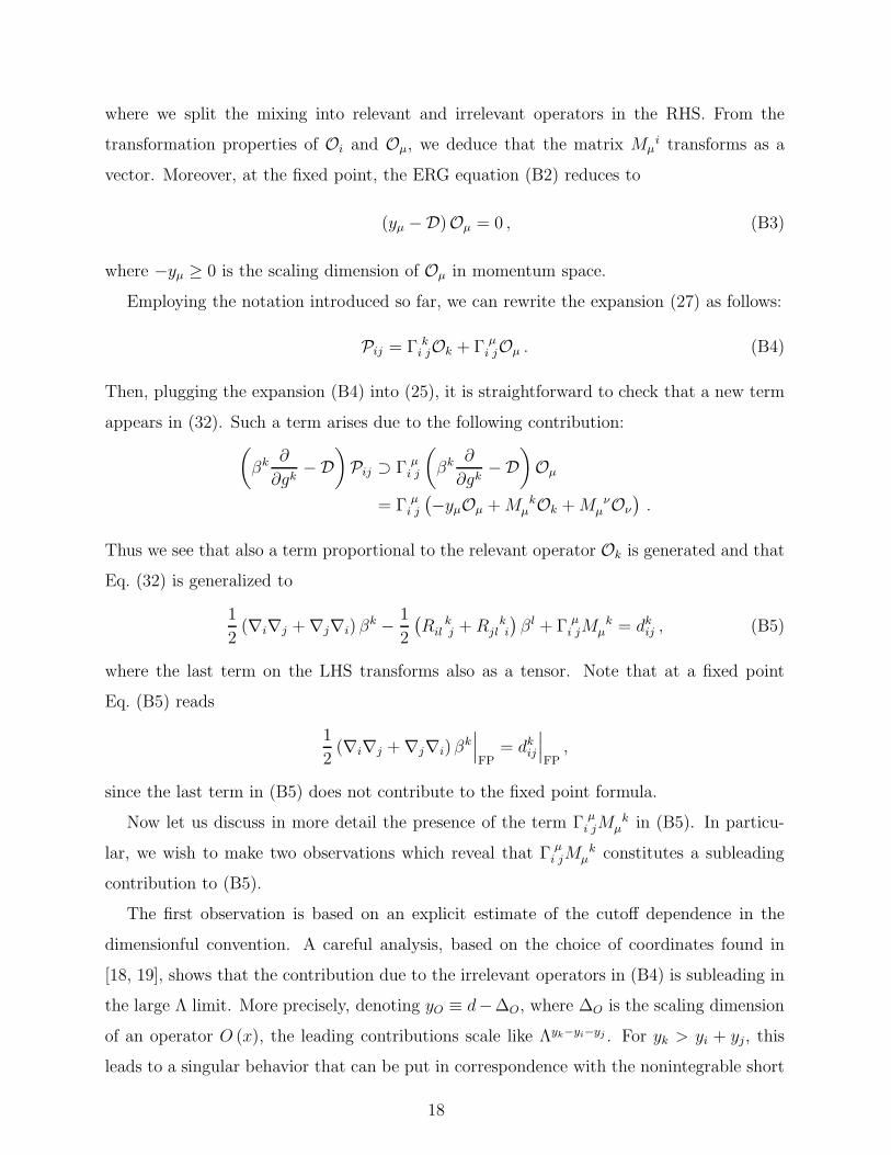
where we split the mixing into relevant and irrelevant operators in the RHS. From the
transformation properties of Oi and Oµ, we deduce that the matrix Mµi transforms as a
vector. Moreover, at the fixed point, the ERG equation (B2) reduces to
(yµ −D)Oµ = 0 , (B3)
where −yµ ≥ 0 is the scaling dimension of Oµ in momentum space.
Employing the notation introduced so far, we can rewrite the expansion (27) as follows:
Pij = Γ ki jOk + Γ µ
i jOµ . (B4)
Then, plugging the expansion (B4) into (25), it is straightforward to check that a new term
appears in (32). Such a term arises due to the following contribution:(
βk ∂
∂gk−D
)
Pij ⊃ Γ µi j
(
βk ∂
∂gk−D
)
Oµ
= Γ µi j
(
−yµOµ +M kµ Ok +M ν
µ Oν
)
.
Thus we see that also a term proportional to the relevant operator Ok is generated and that
Eq. (32) is generalized to
1
2(∇i∇j +∇j∇i) β
k −1
2
(
R kil j +R k
jl i
)
βl + Γ µi jM
kµ = dkij , (B5)
where the last term on the LHS transforms also as a tensor. Note that at a fixed point
Eq. (B5) reads
1
2(∇i∇j +∇j∇i)β
k∣
∣
∣
FP= dkij
∣
∣
∣
FP,
since the last term in (B5) does not contribute to the fixed point formula.
Now let us discuss in more detail the presence of the term Γ µi jM
kµ in (B5). In particu-
lar, we wish to make two observations which reveal that Γ µi jM
kµ constitutes a subleading
contribution to (B5).
The first observation is based on an explicit estimate of the cutoff dependence in the
dimensionful convention. A careful analysis, based on the choice of coordinates found in
[18, 19], shows that the contribution due to the irrelevant operators in (B4) is subleading in
the large Λ limit. More precisely, denoting yO ≡ d−∆O, where ∆O is the scaling dimension
of an operator O (x), the leading contributions scale like Λyk−yi−yj . For yk > yi + yj, this
leads to a singular behavior that can be put in correspondence with the nonintegrable short
18

distance singularities in the OPE via dimensional analysis arguments. The term Γ µi jM
kµ
does not contribute to the singular behavior and can be dropped in (B5) when considering
nonintegrable short distance singularities as it scales like Λ(yµ−yi−yj)<0. This observation
makes evident a link with some previous works in the literature (see in particular [3, 20–
22]), where the nonintegrable short distance singularities are considered, and a geometric
formula fully analogous to (32) is derived.
As a second observation, we note that in order to write down (B5) a certain basis of
irrelevant operators has been selected. If we limit ourselves to consider nonintegrable short
distance singularities, i.e., scaling dimensions such that yk > yi+yj, then the term Γ µi jM
kµ is
dismissed. Hence this truncation has the nice feature of being independent of the convention
chosen for the irrelevant operators.
Appendix C: Cardy’s formula
Let us consider a generic fixed point with N relevant directions. Following [23] we con-
struct the Wilson action perturbatively around the fixed point. Let us denote the relevant
parameters with scale dimension yi > 0 by gi (i = 1, · · · , N). The generating functional
W (g) with an IR cutoff is determined by
N∑
i=1
βi(g)∂
∂gieW (g)[J ] =
∫
p
[(
p · ∂p +D − 2
2+ γ
)
J(p) ·δ
δJ(p)
+ (−p · ∂p + 2− 2γ)R(p) ·1
2
δ2
δJ(p)δJ(−p)
]
eW (g)[J ] . (C1)
Denoting the fixed point functional W ∗ = W (g = 0), we rewrite this in a form more
convenient for perturbative calculations:
N∑
i=1
βi(g)∂
∂gieW (g)−W ∗
=
∫
p
[(
p · ∂p +D − 2
2+ γ
)
J(p)δ
δJ(p)
+ (−p · ∂p + 2− 2γ)R(p) ·
(
δW ∗[J ]
δJ(−p)
δ
δJ(p)+
1
2
δ2
δJ(p)δJ(−p)
)]
eW (g)−W ∗
. (C2)
We assume a constant anomalous dimension γ for simplicity. We wish to solve this pertur-
batively by expanding the functional as
W (g) = W ∗ +
N∑
i=1
giWi +
N∑
i,j=1
1
2gigjWij +
N∑
i,j,k=1
1
3!gigjgkWijk + · · · . (C3a)
19
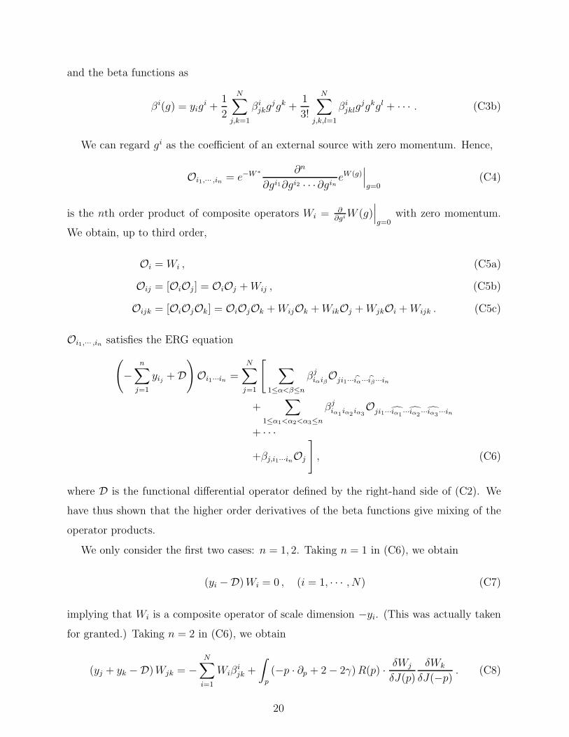
and the beta functions as
βi(g) = yigi +
1
2
N∑
j,k=1
βijkg
jgk +1
3!
N∑
j,k,l=1
βijklg
jgkgl + · · · . (C3b)
We can regard gi as the coefficient of an external source with zero momentum. Hence,
Oi1,··· ,in = e−W ∗ ∂n
∂gi1∂gi2 · · ·∂gineW (g)
∣
∣
∣
g=0(C4)
is the nth order product of composite operators Wi =∂∂gi
W (g)∣
∣
∣
g=0with zero momentum.
We obtain, up to third order,
Oi = Wi , (C5a)
Oij = [OiOj ] = OiOj +Wij , (C5b)
Oijk = [OiOjOk] = OiOjOk +WijOk +WikOj +WjkOi +Wijk . (C5c)
Oi1,··· ,in satisfies the ERG equation
(
−
n∑
j=1
yij +D
)
Oi1···in =
N∑
j=1
[
∑
1≤α<β≤n
βjiαiβ
Oji1···iα···iβ ···in
+∑
1≤α1<α2<α3≤n
βjiα1
iα2iα3
Oji1···iα1
···iα2···iα3
···in
+ · · ·
+βj,i1···inOj
]
, (C6)
where D is the functional differential operator defined by the right-hand side of (C2). We
have thus shown that the higher order derivatives of the beta functions give mixing of the
operator products.
We only consider the first two cases: n = 1, 2. Taking n = 1 in (C6), we obtain
(yi −D)Wi = 0 , (i = 1, · · · , N) (C7)
implying that Wi is a composite operator of scale dimension −yi. (This was actually taken
for granted.) Taking n = 2 in (C6), we obtain
(yj + yk −D)Wjk = −N∑
i=1
Wiβijk +
∫
p
(−p · ∂p + 2− 2γ)R(p) ·δWj
δJ(p)
δWk
δJ(−p). (C8)
20

The integral is local, and we can expand∫
p
(−p · ∂p + 2− 2γ)R(p) ·δWj
δJ(p)
δWk
δJ(−p)=
∞∑
i=1
dijk Oi , (C9)
where Oi = Wi (i = 1, · · · , N), and Oi>N are irrelevant operators of scale dimension −yi ≥ 0.
Hence, we obtain
(yj + yk −D)Wjk =N∑
i=1
Wi
(
dijk − βijk
)
+∑
i>N
dijk Oi . (C10)
In the absence of degeneracy, i.e.,
yj + yk 6= yi (C11)
for any i, j, k ≤ N , we can choose
βijk = 0 (C12)
so that
Wjk =∞∑
i=1
dijkyj + yk − yi
Oi . (C13)
Hence, the beta functions are linear up to second order. This is expected from the old result
of Wegner [23]. (In the absence of degeneracy, the parameters can be chosen to satisfy linear
RG equations.)
Alternatively, we can demand Wjk be free of Wi (i = 1, · · · , N). We must then choose
βijk = dijk . (C14)
We obtain
Wjk =∑
i>N
dijkyj + yk − yi
Oi . (j, k = 1, · · · , N) (C15)
Let g′ i (i = 1, · · · , N) be the choice of parameters for this alternative convention. These are
related to g’s satisfying (C12) as
g′ i = gi +1
2
N∑
j,k=1
dijkyj + yk − yi
gjgk
to order g2. (C14) is a relation very much like what Cardy has obtained using UV regular-
ization in coordinate space [17].
[1] K. G. Wilson and J. B. Kogut, “The Renormalization group and the epsilon expansion,”
Phys. Rept. 12, 75–200 (1974).
21

[2] M. Lassig, “Geometry of the Renormalization GroupWith an Application in Two-dimensions,”
Nucl. Phys. B334, 652–668 (1990).
[3] H. Sonoda, “Connection on the theory space,” in Proceedings of the conference Strings 93,
Berkeley, California, May 24-29, 1993 (World Scientific, 1993) pp. 0154–157.
[4] B. P. Dolan, “Covariant derivatives and the renormalization group equation,”
Int. J. Mod. Phys. A10, 2439–2466 (1995), arXiv:hep-th/9403070 [hep-th].
[5] J. M. Lizana and M. Perez-Victoria, “Wilsonian renormalisation of CFT correlation functions:
Field theory,” JHEP 06, 139 (2017), arXiv:1702.07773 [hep-th].
[6] A. Codello, M. Safari, G. P. Vacca, and O. Zanusso, “Functional perturbative RG and CFT
data in the ǫ-expansion,” (2017), arXiv:1705.05558 [hep-th].
[7] A. Codello, M. Demmel, and O. Zanusso, “Scheme dependence and universality in the func-
tional renormalization group,” Phys. Rev. D90, 027701 (2014), arXiv:1310.7625 [hep-th].
[8] T. R. Morris, “The Exact renormalization group and approximate solutions,”
Int. J. Mod. Phys. A9, 2411–2450 (1994), arXiv:hep-ph/9308265 [hep-ph].
[9] Y. Igarashi, K. Itoh, and H. Sonoda, “On the wave function renormalization for
Wilson actions and their one particle irreducible actions,” PTEP 2016, 093B04 (2016),
arXiv:1607.01521 [hep-th].
[10] O. J. Rosten, “Fundamentals of the Exact Renormalization Group,”
Phys. Rept. 511, 177–272 (2012), arXiv:1003.1366 [hep-th].
[11] C. Pagani and H. Sonoda, “Products of composite operators in the exact renormalization
group formalism,” (2017), arXiv:1707.09138 [hep-th].
[12] H. Sonoda, “Geometrical expression for short distance singularities in field theory,” in Proceed-
ings, 2nd International Colloquium on Modern quantum field theory, Bombay, India, January
5-11, 1994 (World Scientific, 1994) pp. 267–270.
[13] J. Polchinski, “Renormalization and Effective Lagrangians,”
Nucl. Phys. B231, 269–295 (1984).
[14] C. Wetterich, “Exact evolution equation for the effective potential,”
Phys. Lett. B301, 90–94 (1993).
[15] U. Ellwanger, “Flow equations for N point functions and bound states,” Proceedings, Workshop
on Quantum field theoretical aspects of high energy physics: Bad Frankenhausen, Germany,
September 20-24, 1993, Z. Phys. C62, 503–510 (1994).
22
[16] A. Z. Petrov, Einstein spaces, Pergamon Press (1969).
[17] J. L. Cardy, Scaling and Renormalization in Statistical Physics , Cambridge lecture notes in
physics (Cambridge University Press, 1996).
[18] H. Sonoda, “Short distance behavior of renormalizable quantum field theories,”
Nucl. Phys. B352, 585–600 (1991).
[19] H. Sonoda, “The rule of operator mixing,” Nucl. Phys. B366, 629–643 (1991).
[20] H. Sonoda, “Composite operators in QCD,” Nucl. Phys. B383, 173–196 (1992),
arXiv:hep-th/9205085 [hep-th].
[21] H. Sonoda and W.-C. Su, “Operator product expansions in the two-dimensional O(N) non-
linear sigma model,” Nucl. Phys. B441, 310–336 (1995), arXiv:hep-th/9406007 [hep-th].
[22] H. Sonoda and W.-C. Su, “A relation between the anomalous dimensions and
OPE coefficients in asymptotic free field theories,” Phys. Lett. B392, 141–144 (1997),
arXiv:hep-th/9608158 [hep-th].
[23] F. J. Wegner, “Corrections to Scaling Laws,” Phys. Rev. B5, 4529–4536 (1972).
23