Onshore and Offshore Wind Speed Distributions at the ... March 11, 2011, a 9.0 earthquake shocked the ... future planning, ... prediction of atmospheric or space

Abstract—Wind speed data for 2010 at eight stations located

in three coastal areas of Taiwan were used to fit three kinds of

Weilbull distributions in this study. Bimodal Gamma-Weibull

distribution is examined the best among three distributions for

all wind speed data comparing three tests for goodness-of-fit.

Key indicators for a bimodal distribution are the weighting

parameter approaching 0.5, variation of peak speeds of monthly

distribution and peak speed ratio. Topographical effect of high

central mountains of Taiwan on offshore wind speeds at

southern Taiwan is stronger than at northern Taiwan. It

explains that the distribution of offshore wind speeds is bimodal

at northern Taiwan and unimodal at southern Taiwan.

Index Terms—Offshore/onshore wind speed, bimodal

Weibull distribution, goodness-of-fit.

I. INTRODUCTION

On March 11, 2011, a 9.0 earthquake shocked the

northeastern coast of Japan and a tsunami following the

earthquake caused the failure of a nuclear power plant as well

as a massive loss of life and property. Therefore, alternative

power sources instead of nuclear power are again investigated

worldwide. One of several alternative power sources is wind

power that can provide a steady supply of electricity with

clean and sustainable use. Suitable wind farms in Taiwan

were evaluated and many wind turbine generators were

established in coastal areas in the recent ten years. In the

future planning, some offshore wind turbine generators will

be built in the Taiwan Strait. It is important to understand the

characteristics of onshore and offshore in Taiwan waters for

future development of wind power.

Furthermore understanding and modeling wind speed

statistics is a key for a better understanding of atmospheric

turbulence and diffusion and for use in such practical

applications as air quality and pollution transport modeling,

estimation of wind loads on buildings, prediction of

atmospheric or space probe and missile trajectory and wind

power analysis.

Wind speed is a key factor for designing wind power

stations. Statistical analysis on wind speed data around a wind

field is commonly used to study their characteristics,

providing important references for wind energy and

engineering design. Different probability density distribution

of wind speeds has been investigated to show wind power for

the development of wind farms [1]-[7]. The Weibull

distribution is an important distribution especially for

reliability and maintainability analysis.

Both linear least square method and maximum likelihood

method for estimating two Weibull parameters were analyzed

to select locations of installing wind turbine generators [8].

The most accurate and efficient in six numerical methods was

examined to ascertain how closely the measured data follow

the two-parameter Weibull PDF [9]. Wind energy conversion

characteristics of Hatiya Island in Bangladesh were studied

using statistical fitting Weibull distribution for wind speed

data [10]. Wind speed data at three different heights for the

whole year of 2008 at Thasala, southern Thailand were

analyzed using two-parameter Weibull distribution [11]. The

validity domain of the Weibull distribution for wind statistics

was assessed and an alternative expression of more fitted

wind speed distribution was suggested [12].

The Weibull distribution is commonly used for wind speed

data. However, single peak of such a distribution is no more

suitable for two-peak distributed wind speed data. Bimodal

Weibull distribution for wind speeds is examined to be the

best among 14 commonly and previously used probability

density functions for fitting a set of data [13].

The characteristics of offshore winds in Taiwanese waters

have been clarified using in situ coastal wind data for decades.

Three kinds of distributions, i.e. unimodal Weibull, bimodal

Weibull and Gamma-Weibull distributions, are selected to fit

the offshore/onshore wind speeds at eight stations in the

western waters of Taiwan [14]-[16]. T The occurrence

probability and intensity of diurnal and semidiurnal winds

over Taiwanese waters were estimated using wavelet-based

rotary spectral analysis and significance level theory [17].

In order to understand the difference between onshore and

offshore wind speeds for establishment of applicable wind

power stations some Weilbul-like distributions are proposed

for fitting the wind speed data at different stations instead of

single sample in the western waters, Taiwan. he best fitting of

wind speeds among three chosen distributions are determined

by three statistical measures for goodness-of-fit R-Square,

root mean square error and the Kolmogorov-Smirnov test.

The difference between distributions of annual wind speeds

resulting from monthly variation of wind speeds was

indicated. The results can be used as a reference of onshore

and offshore wind energy potentials inthe application to

designing wind power station in Taiwan.

II. BACKGROUND AND DATA

Onshore and Offshore Wind Speed Distributions at the

Western Waters in Taiwan

Jui-Fang Tsai, Hsien-Kuo Chang, Jin-Cheng Liou, and Lian-Sheng Ho

International Journal of Environmental Science and Development, Vol. 7, No. 12, December 2016

867doi: 10.18178/ijesd.2016.7.12.896

Manuscript received December 19, 2015; revised April 7, 2016. This

work was supported in part by the Harbor and Marine Technology Center in

Taiwan under Grant MOTC-IOT-103-H2EB001f .

Jui-Fang Tsai, Hsien-Kuo Chang, and Jin-Cheng Liou are with

Department of Civil Engineering, National Chiao Tung University, Hsinchu

300, Taiwan (e-mail: [email protected], [email protected],

[email protected]).

Lian-Sheng Ho is with Harbor and Marine Technology Center,

Taichung435, Taiwan (e-mail: [email protected]).

Wind speed data at eight stations measured by the Harbor

and Marine Technology Center, Institute of Transportation,

Ministry of Transportation and Communications in Taiwan

were used in this study. These stations are located at the

Taipei harbor in northern Taiwan, the Taichung harbor in

central Taiwan and the Anping harbor in southern Taiwan.

These locations are shown in Fig. 1. Detailed locations and

names of onshore/offshore stations in each area are shown in

Fig. 2.

Fig. 1. Locations of the Taipe, the Taichung and the Anping harbors.

(a) The Taipei harbor

(b) The Taichung harbor (c) The Anping harbor

Fig. 2. Locations of offshore and onshore stations at three harbors of Taiwan.

The wind speeds are measured by Young Brand marine

wind monitor (model 50106). The wind speed sensor is a four

blade helicoid propeller. Propeller rotation produces an AC

sine wave voltage signal with frequency directly proportional

to wind speed. The wind direction sensor is a rugged yet

lightweight vane with a sufficiently low aspect ratio to assure

good fidelity in fluctuating wind conditions. Accuracy of

wind monitor is ±0.3 m/s or 1% for speed and ±3 degrees for

wind direction. Signal output is at a frequency of 1 Hz. Mean

velocity is averaged from all data of instant velocity over

every ten minutes. Hourly data of mean velocity at o’clock

sharp for the whole year are used. Data are transmitted and

collected from the sensor transducer to ground data-base

station through 3G mobile telecommunications every ten

minutes.

Sometimes data in one year are unavailable due to data

transmission or device failure. Except that unavailable data

occur in February at the onshore station of the Taichung

harbor all data at other stations are complete and available for

the whole 2010. Therefore, considering the availability, and

completeness the whole hourly data at eight stations were

used for 2010 in the study.

III. PROBABILITY DENSITY FUNCTION AND MODEL

PERFORMANCE

Weibull distribution:

BUU

Uf

exp),;(1 (1a)

BU

UF

exp1),;(

(1b)

where α is the scale parameter and β is the shape parameter.

Bimodal Weibull distribution:

2

2

2

1

1

1

22

1

2

11

1

12211

exp1

exp,,,,;

UU

UUUf (2a)

2

1

2

1

2211

exp11

exp1,,,,;

U

UUF

(2b)

where the subscripts 1 and 2 indicate the parameters in the

primary part and the second part, respectively, and ω is the

weighting for the primary part.

Gamma-Weibull distribution:

33

33

3

1

3

1

33

exp1

exp)(

),,,,;(

UU

U

k

UkUf

k

k

(3a)

3

3

0

1

33

exp11

)exp)(

1(),,,,;(

U

k

td

Ut

kkUF

U k

(3b)

where Γ(k) is the gamma function evaluated at k, indicating

the shape parameter, and θ is the scale parameter.


868

Weibull, bimodal Weibull and bimodal Gamma-Weibull

distributions, denoted by W, WW and GW, respectively, are

selected for data fitting. WW is examined to be valid for wind

speeds by Morgan et al. [13] and GW is proposed by Chang et

al. [15]. The probability density function (PDF) and

corresponding cumulate probability function (CDF) are

defined as follows:

Three indexes of model performance, the coefficient of

determination, the Kolmogorov-Smirnov test and the root

mean square error are commonly chosen to examine the

goodness of fit of an observed distribution to a theoretical one.

The statistical meaning and definition of these indexes are

given as follows.

The coefficient of determination, R2, shows the ratio of the

variance of the predictions to the sample variance and is

defined as

2

1

2

12

)(

)(

1

YY

yY

RN

ii

i

N

ii

˙ (4)

where Yi and yi are the measurements and predictions,

respectively. R2 ranges from 0 and 1. R

2= 1 indicates that the

regression line perfectly fits the data, while R2= 0 indicates

that the measurements and predictions are independent.

Kolmogorov-Smirnov test (K-S test) is a nonparametric

test of the equality of a continuous probability distribution,

F(U), that can be used to compare a sample with a reference

or empirical probability distribution, E(U), which is obtained

by N ordered data points. The Kolmogorov-Smirnov test

statistic is defined as

))(,1

)((max1

UFN

i

N

iUFD

Ni

(5)

For fitting one data set, a probability distribution having a

smaller D than other distributions indicates that the

distribution is more suitable for fitting the data with an

empirical probability distribution than others.

Root mean square error (RMSE) represents the sample

standard deviation of the differences between predicted

values and observed values. RMSE is a good measure of

accuracy, but only to compare forecasting errors of different

models for a particular variable and not between variables. It

is defined

N

yiYiRMSE

N

i

1

2)( (6)

IV. RESULTS AND DISCUSSION

A. Assessment for Goodness of Fit

In order to assess the goodness of fit of all observed

distributions to three chosen distributions the three statistical

measures were computed for eight cases and list in Table I.

For each case the value of each row in the bold-faced type

indicates the best goodness of fit to such distribution rather

than other two distributions according to such an index. When

a distribution has the most bold-faced values for each case,

the distribution is examined to be the best goodness of fit

among three chosen distributions.

For example, for the case of the offshore station of the

Taipei harbor, three bold-faced values in the first panel of

Table I are list in the last column. The reason is that GW has

smaller values of K-S and RMSE and higher R2 than other two

distributions for such case. Therefore, it is concluded that GW

is a better distribution for fitting wind speeds at the offshore

station of the Taipei harbor than W and WW. For the case of

onshore station A of the Taipei harbor, WW has one

bold-faced K-S value and GW has other two bold-faced

indexes in the second panel. However, the differences of both

values between WW and GW are tiny. Both WW and GW

with equivalent data fitting suitably describe an empirical

probability distribution for such data. Three bold-faced

indexes are all list in the second column in the third panel. The

result indicates that the best data fitting for the distribution is

WW for the case of the onshore station B of the Taipei harbor.

For the Taichung harbor, all best indexes list in the second

column of the second panel show that distributed data at the

offshore station can be better fitted by WW rather than by W

and GW. Best indexes being in the third column indicate that

the distribution of wind speeds can be suitably fitted by GW at

the onshore station A. At the onshore station B, WW and GW

are equivalently valid for the distribution of wind speeds.

For the Anping harbor, all indexes are list in the last panel

of Table I. The distribution of wind speeds at offshore and

onshore stations can be more validly fitted by GW than by W

and WW. W is the worst one to fit the distribution of wind

speeds among three distributions for all data sets. From the

above discussion WW is suggested for the distribution of

wind speeds at onshore stations B of the Taipei harbor and for

those at offshore stations of the Taichung harbor. For other

stations GW is suggested for the distribution of wind speeds.

TABLE I: THREE STATISTICAL TESTS FOR THE GOODNESS OF FIT OF ALL

DATA DISTRIBUTIONS TO THE W, WW AND GWD IS ATTRIBUTIONS

Harbor Station Index W WW GW

Taipei

Offshore

R2 0.9023 0.9865 0.9968

K-S

RMSE

0.0535

0.0122

0.0182

0.0044

0.0099

0.0022

On- A

R2 0.9848 0.9963 0.9968

K-S

RMSE

0.0243

0.0163

0.0191

0.0076

0.0201

0.0069

On-B

R2 0.9981 0.9999 0.9999

K-S

RMSE

0.0304

0.0073

0.0086

0.0027

0.0093

0.0030

Taichun

g

Offshore

R2 0.9807 0.9905 0.9845

K-S

RMSE

0.0300

0.0040

0.0162

0.0029

0.0201

0.0037

On- A

R2 0.9076 0.9862 0.9892

K-S

RMSE

0.0583

0.0158

0.0183

0.0064

0.0174

0.0060

On-B

R2 0.9981 0.9981 0.9982

K-S

RMSE

0.0086

0.0024

0.0086

0.0025

0.0098

0.0024

Anping

Offshore

R2 0.9853 0.9919 0.9950

K-S

RMSE

0.0226

0.0062

0.0230

0.0044

0.0091

0.0035

Onshore

R2 0.9967 0.9882 0.9958

K-S

RMSE

0.0336

0.0124

0.0243

0.0075

0.0085

0.0044

GW is finally chosen to investigate the data fitting in

further study. The obtained values of parameters in GW for all

data are list in Table II. Through the parameters of the

Gamma and Weibull distributions associated with weighting

ω in Table II, the whole distribution can be separated into the


869

primary Gamma part and second Weibull part.

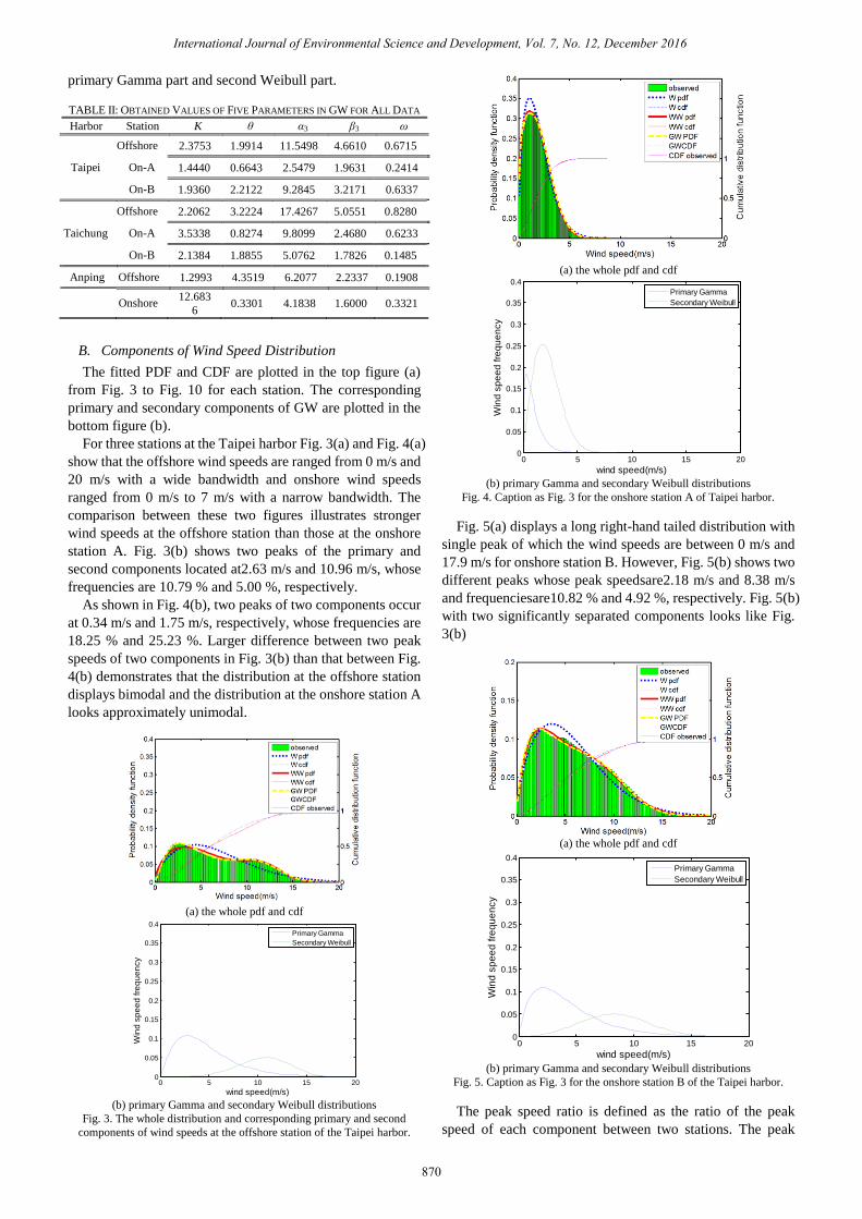
TABLE II: OBTAINED VALUES OF FIVE PARAMETERS IN GW FOR ALL DATA

Harbor Station K θ α3 β3 ω

Taipei

Offshore 2.3753 1.9914 11.5498 4.6610 0.6715

On-A 1.4440 0.6643 2.5479 1.9631 0.2414

On-B 1.9360 2.2122 9.2845 3.2171 0.6337

Taichung

Offshore 2.2062 3.2224 17.4267 5.0551 0.8280

On-A 3.5338 0.8274 9.8099 2.4680 0.6233

On-B 2.1384 1.8855 5.0762 1.7826 0.1485

Anping Offshore 1.2993 4.3519 6.2077 2.2337 0.1908

Onshore

12.683

6 0.3301 4.1838 1.6000 0.3321

B. Components of Wind Speed Distribution

The fitted PDF and CDF are plotted in the top figure (a)

from Fig. 3 to Fig. 10 for each station. The corresponding

primary and secondary components of GW are plotted in the

bottom figure (b).

For three stations at the Taipei harbor Fig. 3(a) and Fig. 4(a)

show that the offshore wind speeds are ranged from 0 m/s and

20 m/s with a wide bandwidth and onshore wind speeds

ranged from 0 m/s to 7 m/s with a narrow bandwidth. The

comparison between these two figures illustrates stronger

wind speeds at the offshore station than those at the onshore

station A. Fig. 3(b) shows two peaks of the primary and

second components located at2.63 m/s and 10.96 m/s, whose

frequencies are 10.79 % and 5.00 %, respectively.

As shown in Fig. 4(b), two peaks of two components occur

at 0.34 m/s and 1.75 m/s, respectively, whose frequencies are

18.25 % and 25.23 %. Larger difference between two peak

speeds of two components in Fig. 3(b) than that between Fig.

4(b) demonstrates that the distribution at the offshore station

displays bimodal and the distribution at the onshore station A

looks approximately unimodal.

(a) the whole pdf and cdf

0 5 10 15 200

0.05

0.1

0.15

0.2

0.25

0.3

0.35

0.4

wind speed(m/s)

Win

d s

pe

ed

fre

qu

en

cy

Primary Gamma

Secondary Weibull

(b) primary Gamma and secondary Weibull distributions

Fig. 3. The whole distribution and corresponding primary and second

components of wind speeds at the offshore station of the Taipei harbor.


0 5 10 15 200

0.05

0.1

0.15

0.2

0.25

0.3

0.35

0.4

wind speed(m/s)

Win

d s

pe

ed

fre

qu

en

cy

Primary Gamma

Secondary Weibull


Fig. 4. Caption as Fig. 3 for the onshore station A of Taipei harbor.

Fig. 5(a) displays a long right-hand tailed distribution with

single peak of which the wind speeds are between 0 m/s and

17.9 m/s for onshore station B. However, Fig. 5(b) shows two

different peaks whose peak speedsare2.18 m/s and 8.38 m/s

and frequenciesare10.82 % and 4.92 %, respectively. Fig. 5(b)

with two significantly separated components looks like Fig.

3(b)


0 5 10 15 200

0.05

0.1

0.15

0.2

0.25

0.3

0.35

0.4

wind speed(m/s)

Win

d s

pe

ed

fre

qu

en

cy

Primary Gamma

Secondary Weibull


Fig. 5. Caption as Fig. 3 for the onshore station B of the Taipei harbor.

The peak speed ratio is defined as the ratio of the peak

speed of each component between two stations. The peak


870

frequency ratio is the ratio of the peak frequency of each

component between two stations. Two peak speed ratios

between the offshore station and the onshore station A are7.73

and 6.26, respectively. The peak frequency ratios are 0.59 and

0.19, respectively. Two peak speed ratios and corresponding

peak frequency ratios between the offshore station and the

onshore station B are 1.20 and 1.30, respectively, and 0.99

and 1.01, respectively.


0 5 10 15 20 25 300

0.05

0.1

0.15

0.2

wind speed(m/s)

Win

d s

pe

ed

fre

qu

en

cy

Primary Gamma

Secondary Weibull


Fig. 6. Caption as Fig. 3 for the offshore station of the Taichung harbor.

Three weightings of GW in Table I are 0.6715, 0.2414 and

0.6337, respectively. When the weighting of a binomial

distribution is close to 1 or zero, the primary component is

significantly larger or smaller than the other second

component. The whole distribution has a single peak. The

weighting close to 0.5 implies that both components are

equivalent and the whole distribution displays bimodal. The

weightings of the offshore and the onshore station B

approaching 0.6 explain why both distributions are bimodal.

By two components of a bimodal distribution and peak

speed ratio as well as peak frequency ration it is easy to

explain the reason that the difference between distributions of

the offshore station and of the onshore station A at the Taipei

harbor is large, but small between and the offshore station and

of the onshore station B. The onshore station A is 5 km away

from the coast and near northeastern hill. In the winter

monsoons are strong winds blowing northeast wards. Because

of topographical sheltering reduced wind speeds at the

onshore station A are measured. On the other hand, onshore

station B is located at the end of northern breakwaters of the

Taipei harbor. There are no obstacles to change the offshore

winds, and the wind speed and probability density distribution

are similar to those of the offshore station.

For three stations at the Taichung harbor, Fig. 6(a), Fig. 7(a)

and Fig. 8(a) show that the offshore wind speeds are ranged

from 0 m/s and 25.60 m/s and onshore wind speeds ranged

from 0 m/s to 19.50 m/s, and 0 m/s to 14.94 m/s, respectively,

for station A and B. Three fitted probability density functions

appear unimodal and right-hand tailed, special at the offshore

station and the onshore station B.

Three weightings of GW in Table I are 0.8280, 0.6233 and

0.1485, respectively. The weightings of the offshore and the

onshore station B deviating from 0.5 implying that both

distributions should seem unimodal.

Fig. 6(b) shows two peaks of the primary and second

components located at 3.82 m/s and 16.64 m/s, whose

frequencies are 8.72 % and 1.87 %, respectively. As shown in

Fig. 7(b), two peaks of two components occur at 2.08 m/s and

7.88 m/s, respectively, whose frequencies are 18.27 % and

3.83%. Fig. 8(b) shows two peaks of the primary and second


frequencies are 2.73 % and 13.42 %, respectively.

Two peak speed ratios between the offshore station and the

onshore station A are 1.83 and 2.11, respectively. The

corresponding peak frequency ratios are 0.47 and 0.48,

respectively. Two peak speed ratios and corresponding peak

frequency ratios between the offshore station and the onshore

station B are 1.71 and 5.05, respectively, and 3.19 and 0.13,

respectively.


0 5 10 15 20 25 300

0.05

0.1

0.15

0.2

wind speed(m/s)

Win

d s

pe

ed

fre

qu

en

cy

Primary Gamma

Secondary Weibull


Fig. 7. Caption as Fig. 3 for the onshore station A of the Taichung harbor.

For two stations at the Anping harbor, Fig. 9(a) and Fig.

10(a) indicate that the offshore wind speeds are ranged from 0

m/s and 18 m/s and onshore wind speeds ranged from 0 m/s to

12.8 m/s. Two weightings in the third panel in Table I are

0.1908 and 0.3321, respectively. The weighting of the

offshore approaching zero shows the distribution unimodal.

The other distribution at the offshore should appear

insignificantly bimodal.

Fig. 9(b) shows two peaks of the primary and second


frequencies are 2.47 % and 12.07 %, respectively. It is shown

in Fig. 10(b) that two peak speeds are3.90 m/s and 2.29 m/s,

respectively, whose frequencies are11.65 % and 12.15 %.


871

Two peak speed ratios between the offshore station and the

onshore station are 0.22 and 2.04, respectively. The

corresponding peak frequency ratios are 0.21 and 0.99,

respectively.


0 5 10 15 20 25 300

0.05

0.1

0.15

0.2

wind speed(m/s)

Win

d s

pe

ed

fre

qu

en

cy

Primary Gamma

Secondary Weibull


Fig. 8. Caption as Fig. 3 for the onshore station B of the Taichung harbor.



Fig. 9. Caption as Fig. 3 for the offshore station of the Anping harbor.

Strong northeastern winds blow during the winter in

Taiwan. High central mountains with the tallest peak being

3952 m, running from the north of the island to the south in

Taiwan, weaken the monsoons. Therefore, the wind speeds at

the offshore station differ insignificantly from those at the

onshore of the Anping harbor.



Fig. 10. Caption as Fig. 3 for the onshore station of the Anping harbor.

(a) surface plot

C. Monthly Distribution of Wind Speeds

In the above sub-section, the weighting parameter and

components of a distribution are used to demonstrate the

characteristics of a bimodal wind speed distribution. However,

the distribution of wind speeds is obtained from data of the

whole year. We attempt to explain the reason why the two

peak speeds occur. Twelve distributions of monthly wind

speeds of the offshore stations at three harbors are plotted in


872

(b) contour plot

Fig. 11. Monthly distribution of wind speeds at the offshore station of the

Taipei harbor.

surface plot and contourplot, respectively, and shown in Fig.

11 to Fig. 13.

(a) surface plot

(b) contour plot

Fig. 12. Caption as Fig. 11 for the Taichung harbor.

(a) surface plot

(b) contour plot

Fig. 13. Caption as Fig. 11 for theAnping harbor.

Fig. 11 indicates that monthly peak wind speeds are about

10 m/s during winter time from September to March next year

and are about 3 m/s during the summer time from April to

August. Monthly peak wind speeds in the winter significantly

differ from those in the summer. Occurrence frequencies of

both kinds of monthly peak velocity are approximate.

Different wind speeds in the winter and in the summer result

in a bimodal distribution of the whole wind speeds.

For the Taichung harbor Fig. 12 shows that monthly peak

wind speeds vary in a range of 3 m/s to 8 m/s during the

periods from February to November and about 13 m/s for

January and December. Due to various monthly peaks over

long time the distribution of the whole wind speeds with a

long right-land tail is wide but non-obviously bimodal.

Twelve peak wind speeds of the monthly distribution,

shown in Fig. 13, of the Anping harbor vary from 3 m/s to6

m/s. The result indicates the distribution of the whole wind

speeds having a single peak and being narrow banded.

V. CONCLUSION

Data of wind speeds at eight onshore or offshore stations at

the western waters in Taiwan for the whole year were fitted by

single peak and bimodal distributions. Some conclusions are

made and list below:

1) Three tests for goodness-of-fit of three chosen

distributions are examined to show that the bimodal

Gamma-Weibull is most valid for most data sets.

2) The weighting parameter in the bimodal Gamma-Weibull

distribution approaching 0.5 is a key index for

distinguishable peaks.

3) Ratios of two peak speeds and frequencies of the primary

and the secondary components is an alternative index to

explain why a distribution is bimodal.

4) Small variation of peak speeds and frequencies of

monthly distribution shows single peak distribution of the

whole wind speeds. Contrarily large variation of monthly

peaks indicates a two-peaked distribution.

Based on the understanding of onshore and offshore wind

speed data in Taiwanese western waters, the diurnal and

semidiurnal oscillations in surface wind as well as the

seasonal and spatial characteristics of these oscillations

should be further investigated. The effects of such variations

on offshore wind energy conversion are considerable and

should not be ignored. The shafts of offshore wind turbines

with long blades are commonly settled at a height of more

than 90 m above the seas, the characteristics of vertically

distributed wind speeds instead of those at single point are

important to accurately determine energy efficiency of wind

turbine in the further study.

REFERENCES

[1] F. Y. Ettoumi, H. Sauvageot, and A. E. H. Adane, “Statistical bivariate

modelling of wind using first-order Markov chain and Weibull

distribution,” Renewable Energy, vol. 28, pp. 1787-1802, 2003.

[2] J. D. Holmes and W. W. Moriarty, “Application of the generalized

Pareto distribution to extreme value analysis in wind engineering,”

Journal of Wind Engineering and Industrial Aerodynamics, vol. 83,

pp. 1-10, 1999.

[3] O. A. Jaramillo and M. A.Borja, “Wind speed analysis in La Ventosa,

Mexico: a bimodal probability distribution case,” Renewable Energy,

vol. 29, pp. 1613-1630, 2004.

[4] M. Li and X. Li, “MEP-type distribution function: a better alternative

to Weibull function for wind speed distributions,” Renewable Energy,

vol. 30, pp. 1221-1240, 2005.

[6] J. Zhou, E. Erdem, G. Li, and J. Shi, “Comprehensive evaluation of

wind speed distribution models: A case study for North Dakota sites,”

Energy Conversion and Management, vol. 51, pp. 1449-1458, 2010.

[7] I. Usta and Y. M. Kantar, “Analysis of some flexible families of

distributions for estimation of wind speed distributions,” Applied

Energy, vol. 89, pp. 355-367, 2012.


873

[5] Y. O. Xiao, Q. S. Li, Z. N. Li, and G.Q. Li, “Probability distributions of

extreme wind speed and its occurrence interval,” Engineering

Structures, vol. 28, pp. 1173-1181, 2006.

[8] P. Bhattacharya and R. Bhattacharjee, “A study on Weibull

distribution for estimating the parameters,” Journal of Applied

Quantitative Methods, vol. 5, pp. 234-241, 2010.

[9] D. K. Kidmo, R. Danwe, S. Y. Doka, and N. Djongyang, “Statistical

analysis of wind speed distribution based on six Weibull methods for

wind power evaluation in Garoua, Cameroon,” Revue des Energies

Renouvelables, vol. 18, pp. 105-125, 2015.

[10] A. K. Azada et al., “Analysis of wind energy conversion system using

Weibulldistribution,” Procedia Engineering, vol. 90, pp. 725-732,

2014,

[11] J. Waewsak, C. Chancham1, M. Landry, and Y. Gagnon, “An analysis

of wind speed distribution at Thasala, Nakhon Si Thammarat,

Thailand,” Journal of Sustainable Energy & Environment, vol. 2, pp.

51-55, 2011.

[12] P. Drobinski and C. Coulais, “Is the Weibull distribution really suited

for wind statistics modeling and wind power evaluation?”

[13] E. C. Morgan, M. Lackner, R. M. Vogel, and L. G. Baise, “Probability

distributions for offshore wind speeds,” Energy Conversion and

Management, vol. 52, pp. 15-26, 2011.

[14] T. P. Chang, “Estimation of wind energy potential using different

probability density function,” Applied Energy, vol. 88, pp. 1848-56,

2011.

[15] T. P. Chang, “Wind speed and power density analyses based on

mixture weibull and maximum entropy distributions,” International

Journal of Applied Science and Engineering, vol. 1, pp. 39-46, 2010.

[16] F.J. Liu, H. H .Ko, S. S. Kuo, Y. H. Liang, and T. P. Chang, “Study on

wind characteristics using bimodal mixture weibull distribution for

three wind sites in Taiwan,” Journal of Applied Science and

Engineering, vol. 17, pp. 283-292, 2014.

[17] H. Chien, H. Y. Cheng, K. H. Yang, Y. H. Tsai, and W. T. Chang,

“Diurnal and semidiurnal variability of coastal wind over Taiwanese

waters,” Wind Energy, vol. 18, pp. 1353–1370, 2014.

Jui-Fang Tsai was born in 1977. He is a PhD student

of civil engineering in National Chiao Tung

University, Taiwan. His current research interests

about numerical model and statistical model of wind.

Hsien-Kuo Chang was born in 1960. He received his

PhD degree in hydraulic and ocean engineering from

Cheng Kung University. He is currently a professor of

Civil Engineering in National Chiao Tung University.

He specializes in coastal engineering, remote sensing

and wave mechanics.

Jin-Cheng Liou was born in 1975. He received his

PhD degree in civil engineering from National Chiao

Tung University, Taiwan, in 2005. He worked as a

postdoctoral fellow at the Department of Civil

Engineering in National Chiao Tung University,

Taiwan. His current research interests are in

oceanography numerical model and wave mechanics.

Lian-Sheng Ho received his PhD degree in hydraulic

and ocean engineering from Cheng Kung University.

He is currently a section chief of Harbor and Marine

Technology Center, Taiwan. He specializes in coastal

engineering and spectral analysis.


874

Documents

Onshore and Offshore Wind Speed Distributions at the ... March 11, 2011, a 9.0 earthquake shocked the ... future planning, ... prediction of atmospheric or space