Onset of convection with ﬂuid compressibility and ... Pub/MyintFiroozabadiPoF2013a.pdf · PHYSICS OF FLUIDS25,094105(2013) Onset of convection with ﬂuid compressibility and interface

PHYSICS OF FLUIDS 25, 094105 (2013)

Onset of convection with fluid compressibilityand interface movement

Philip C. Myint1,2,a) and Abbas Firoozabadi1,3,b)1Department of Chemical and Environmental Engineering, Yale University,9 Hillhouse Avenue, New Haven, Connecticut 06511, USA2Atmospheric, Earth, and Energy Division, Lawrence Livermore National Laboratory,Livermore, California 94550, USA3Reservoir Engineering Research Institute, Palo Alto, California 94301, USA

(Received 28 June 2013; accepted 5 September 2013; published online 25 September 2013)

The density increase from carbon dioxide (CO2) dissolution in water or hydrocar-bons creates buoyancy-driven instabilities that may lead to the onset of convection.The convection is important for both CO2 sequestration in deep saline aquifers andCO2 improved oil recovery from hydrocarbon reservoirs. We perform linear stabilityanalyses to study the effect of fluid compressibility and interface movement on theonset of buoyancy-driven convection in porous media. Compressibility relates to anon-zero divergence of the velocity field. The interface between the CO2 phase andthe aqueous or hydrocarbon phase moves with time as a result of the volume changethat occurs upon CO2 dissolution. Previous stability analyses have neglected thesetwo aspects by assuming that the aqueous or hydrocarbon phase is incompressibleand that the interface remains fixed in position. The stability analyses are used tocompute two key quantities: (1) the critical time and (2) the critical wavenumber. Ourresults indicate that compressibility has a negligible effect on the critical time and thecritical wavenumber in CO2-water mixtures. We use thermodynamics to derive anexpression which shows that the two opposing physical processes which contributeto the divergence are comparable in magnitude and largely cancel each other. Thisresult explains why compressibility does not significantly affect the onset, and it alsodemonstrates the link between compressibility and the volume change that causesmovement of the interface. Compared to when the interface is fixed in position, amoving interface in CO2-water mixtures may reduce the critical time by up to around10%, which can be significant in low permeability formations. The decrease in thecritical time due to interface movement may be much more pronounced in hydro-carbons than in water. This could have important implications for CO2 improved oilrecovery. C! 2013 AIP Publishing LLC. [http://dx.doi.org/10.1063/1.4821743]

I. INTRODUCTION

Global energy demand from fossil fuels is expected to remain over 70% in the coming decades,despite considerable efforts to develop alternative energy sources.1 Combustion of fossil fuelscontributes to rising atmospheric carbon dioxide (CO2) levels that have been linked to climatechange. Subsurface CO2 injection can help society meet its high demand for fossil fuels and reduceatmospheric CO2 levels. Carbon dioxide has been employed for over four decades in improved oilrecovery.2, 3 Dissolution of CO2 in oil may reduce the viscosity by over an order of magnitude andmay increase the volume of the resulting mixture by up to 60%. The volume expansion helps to expelthe oil from smaller porous cavities. Within the past two decades, CO2 injection for sequestration indeep saline aquifers has received considerable attention as a promising way to reduce atmospheric

a)Electronic mail: [email protected])Electronic mail: [email protected]

1070-6631/2013/25(9)/094105/16/$30.00 C!2013 AIP Publishing LLC25, 094105-1

Downloaded 25 Sep 2013 to 130.132.173.174. This article is copyrighted as indicated in the abstract. Reuse of AIP content is subject to the terms at: http://pof.aip.org/about/rights_and_permissions

http://dx.doi.org/10.1063/1.4821743

http://dx.doi.org/10.1063/1.4821743

http://dx.doi.org/10.1063/1.4821743

http://crossmark.crossref.org/dialog/?doi=10.1063/1.4821743&domain=pdf&date_stamp=2013-09-25

094105-2 P. C. Myint and A. Firoozabadi Phys. Fluids 25, 094105 (2013)

CO2 levels.4–6 This process involves capturing CO2 emissions from stationary sources, such as powerplants, and storing the CO2 by dissolving it in the aqueous phase that resides in the aquifers. The CO2

is usually injected at supercritical conditions and forms a free phase because CO2 is only partiallymiscible with the in situ aqueous or hydrocarbon phase. We refer to the aqueous or hydrocarbonphase collectively as the liquid phase. The CO2 phase is typically lighter than the liquid phase, andit initially mixes with the underlying liquid only by diffusion.

Carbon dioxide is the only common atmospheric gas that increases the density of hydrocarbonsupon dissolution,7 and one of the few that increases the density of water.8 The density increasecreates an unstable situation where heavier, CO2-dissolved fluid lies on top of lighter fluid. Theinstabilities may lead to the onset of buoyancy-driven convection in the liquid phase. Convection isof great interest because it strongly enhances the CO2 dissolution rate over diffusion alone. In thisway, it increases the efficiency of improved oil recovery processes. However, the convection may alsolead to earlier appearance of CO2 in the production well, which is an undesirable consequence thatmust be monitored in field-scale operations.9, 10 Convection not only increases the storage efficiencyof CO2 sequestration, it also has implications for the long-term storage security of the CO2. Theenhanced dissolution of CO2 into the aqueous phase reduces the pressure buildup in the free CO2

phase. The pressure reduction makes it less likely that the cap rock enclosing the aquifer will fracture,which lowers the risk of CO2 leakage back into the atmosphere. Thus, convection is important forboth CO2 improved recovery and CO2 sequestration, and it is of interest to determine the conditionsunder which the instabilities may lead to the onset of convection in the liquid phase.

Several authors have performed a linear stability analysis to theoretically predict the onsetof buoyancy-driven convection in the context of CO2 sequestration.11–16 Their work has been ex-tended to include features such as hydrodynamic dispersion,17 temperature gradients,18, 19 chemicalreactions,20, 21 and permeability anisotropy.22–24 The state of the system before the onset of con-vection, when CO2 is transported through the liquid phase only by diffusion, is referred to as thebase state. The stability analysis is a semi-analytical method that introduces small wave-like pertur-bations to the base state in order to determine the conditions under which the base state becomesunstable. The stability analysis is used to calculate two key quantities: (1) the critical time and(2) the critical wavenumber. Onset of convection occurs at the critical time, which represents thefirst instance when the base state becomes unstable. The critical wavenumber characterizes themost unstable perturbation mode. There have also been a number of numerical simulations25–29 andlaboratory-scale experiments30–32 regarding CO2 sequestration. However, simulations and experi-ments focus on the time when the average CO2 concentration in the liquid phase begins to deviatefrom the diffusion-only profile. This time may be quite distinct from the critical time and is an aspectof convection that is not examined by the stability analysis, which investigates only the onset ofinstability.16, 24, 29

The aforementioned linear stability analyses have employed a common set of assumptions. Forexample, various authors consider a situation where enough CO2 has been injected into the subsurfaceto form a reservoir that keeps the interface between the CO2 phase and the liquid phase saturatedat a constant CO2 concentration. The studies have examined the dynamics in only the liquid phasebecause the solubility of water or hydrocarbons in CO2 is assumed to be small compared to the CO2

solubility in the liquid phase. Evaporation of liquid is neglected. These are good approximationsat relatively low temperatures and high pressures. Other assumptions may not be as valid. Forinstance, the liquid phase is treated as being incompressible, and the change in its volume due toCO2 dissolution is neglected so that the interface remains fixed in position. Compressibility relatesto a non-zero divergence of the velocity field. The maximum possible volume change, which isknown as swelling, corresponds to when the liquid phase is saturated with CO2 at the equilibriumconcentration. Swelling may be quite significant under relevant conditions of temperatures between30 and 200 !C and pressures up to 200 bars. The solubility of CO2 in water can be as high as 8 masspercent under these conditions,33 and swelling can be as much as 7%. Under the same conditions,the solubility of CO2 in hydrocarbons can be as high as 50 mass percent, and swelling can be asmuch as 60%.2

In this paper, we perform linear stability analyses to examine the effect of fluid compressibilityand interface movement on the onset of buoyancy-driven convection. Previous stability analyses



have neglected the former, while the effect of interface movement has been examined only recentlyby Meulenbroek et al.34 We address fluid compressibility in Sec. II. We analyze how the non-zero divergence affects the critical time and critical wavenumber. We use thermodynamics to deriveexpressions for the two physical processes that contribute to the divergence. This allows us to achievetwo purposes: (1) gain insight into our results regarding compressibility, and (2) demonstrate the linkbetween compressibility and the volume change from CO2 dissolution, i.e., the moving interface.Section III presents a stability analysis with the moving interface. We compare our results to thoseobtained by Meulenbroek et al.34 Our work is applicable to both CO2 improved oil recovery andCO2 sequestration, but for clarity and for reasons mentioned later, we focus mainly on the latter.In the appropriate sections, we discuss how compressibility and interface movement may be morepronounced in hydrocarbons than in water. We conclude with a summary of our main resultsin Sec. IV.

II. FLUID COMPRESSIBILITY

A. Governing and constitutive equations

Our system is an isothermal binary mixture of CO2 and water (or a liquid hydrocarbon) residingin an inert, permeable, rectangular medium of height H that is homogeneous and isotropic in itsporosity ! and permeability k. The z axis is centered at the interface, which forms the top boundary,and points upward so that porous domain is defined between z = "H at the bottom and z = 0 at theinterface. The viscosity µ and diffusion coefficient D are constants. The diffusive flux is given byFick’s law as J = "!"D#c, where " is the mass density and c is the CO2 mass fraction. Fluid flowis governed by Darcy’s law which relates the velocity field q = (u, v, w)T to the pressure gradient#p and the gravitational force ""g#z. We also have the continuity equation and a CO2 speciesbalance. These equations may be expressed, respectively, as

q = " kµ

(# p + "g#z) , (1)

!#"

#t+ # · ("q) = 0, (2)

!#c"#t

= "# · (c"q) + !D# · ("#c) . (3)

Substituting (2) into (3), we obtain!

!#

#t+ q · #

"c = dc

dt= !D

!1"

#" · #c + #2c"

, (4)

where d/dt = !#/#t + q · # denotes the total time derivative (or material derivative) operator. Thedensity obeys the constitutive equation used in previous studies

" = "0(1 + $c). (5)

We have previously shown24 that (5) is a Taylor series approximation about c = 0 at a particularpressure p. Its validity depends on the specific fluid mixture and the conditions considered. Theequation is accurate for CO2-water mixtures under the conditions mentioned in Sec. I. The densityof pure water (or hydrocarbon) is "0. We show in Sec. II D that "0 and $ depend on temperature,but are nearly invariant with respect to pressure and composition so that they may be approximatedas being constants in our isothermal system. As a result, (5) is linear in c. Using (5) and lettingP = p + "0gz, (1) becomes

q = " kµ

(# P + "0$cg#z) . (6)

The liquid side of the interface is saturated with CO2 at a fixed mass fraction csat. Initially, CO2 ispresent only at the interface, and the bulk is pure water (or hydrocarbon). The maximum increase in



density from CO2 dissolution is %" = "0$csat. It is less than 2% of "0 for CO2-water mixtures, butit can be as high as several percent of "0 for CO2-hydrocarbons.35 Rearranging (2) gives

# · q = " 1"

d"

dt. (7)

Since " = "(T, p, c), the temperature T is a constant, and #"/#p $ 0, we have

# · q = " 1"

#"

#cdcdt

= ""0$

"

dcdt

.

Substituting (4), we get

# · q = "!D"0$

"

!1"

#" · #c + #2c"

. (8)

Equation (8) shows that the divergence of q at a point in space is proportional to the divergence ofthe diffusive flux at that point. We follow earlier works13, 16, 26 and nondimensionalize our equationswith a velocity scale ! = k%"g/µ, a length scale & = (!D)/! = (D!µ)/(k%"g), and a time scale' = (!&)/! = D [(!µ)/(k%"g)]2. We define the dimensionless variables

(x, y, z)T = 1&

(x, y, z)T ,

q = (u, v, w)T = 1!

(u, v, w)T ,

t = 1'

t, c = 1csat

c, P = 1%"g&

P.

In nondimensional terms, the quantity in parentheses on the right hand side of (4) or (8) is(csat/&

2)[(%"/")|# c|2 + #2c]. The (%"/")|# c|2 term is negligible compared to #2c because|# c|2 = # c · # c is on the same order as #2c, but %" % ". We use this approximation and nondi-mensionalize (4), (6), and (8) to get

# c#t

= "q · # c + #2c, (9)

q = "# P " c# z, (10)

# · q = "%"

"#2c. (11)

In this choice of scaling, the Rayleigh number Ra = H/& = (k%"gH)/(!µD) does not appear inthe governing equations. Instead, Ra appears in the location of the bottom boundary so that porousdomain is defined in the range "Ra & z & 0. At the onset of convection, the CO2 concentrationwill be small at the bottom boundary for sufficiently tall domains. This implies that the bottomboundary becomes irrelevant for large enough values of H. Slim and Ramakrishan16 have shownthat the results of the stability analysis are independent of the Rayleigh number for domains whereRa > 75.

B. The base state

The base state is characterized by a pressure field Pbase and the absence of bulk fluid motion(qbase = 0). The CO2 concentration profile cbase(z, t) of the base state obeys

# cbase

# t= #2cbase

# z2. (12)

We stated in Sec. II A that the bottom boundary of the porous domain is irrelevant for our problem.To simplify the calculations, we treat the domain as a semi-infinite medium where "' < z & 0.



The initial/boundary conditions are

cbase(z, t = 0) = 0, "' < z < 0, (13)

cbase(z ( "', t) = 0, )t, (14)

cbase(z = 0, t) = 1, )t . (15)

The solution to (12) with the initial/boundary conditions (13)–(15) is

cbase(z, t) = 1 + erf(z/2*

t), (16)

where erf(x) is the error function.16 Applying Leibniz’s rule to (16) yields

# cbase

# z= 2*

(exp

!"z2

4t

"#

# z

!z

2*

t

"= 1*

( texp

!"z2

4t

", (17)

#2cbase

# z2= " z

2(( t3)1/2exp

!"z2

4t

". (18)

C. Linearized perturbation equations

1. Formulation

The perturbations to the base state are defined as

q + = q =#u+, v+, w+$T

, (19)

P + = P " Pbase, (20)

c+ = c " cbase. (21)

We substitute (19)–(21) into (9)–(11) and linearize the equations (neglect products of perturbations)to obtain

# c+

# t= "w+ # cbase

# z+ #2c+, (22)

q + = "# P + " c+# z, (23)

# · q + = "%"

"

!#2c+ + #2cbase

# z2

". (24)

Following previous work,11–16 we eliminate P +, u+, and v+ by taking twice the curl of (23), usingthe identity # , # , q + = #(# · q +) " #2q +, applying (24), and equating the vertical componentsto obtain

#2w+ = "#2h c+ " #

# z

%%"

"

!#2c+ + #2cbase

# z2

"&, (25)

where #2h = #2/# x2 + #2/# y2 is the horizontal Laplacian. Using (5) with the quantities %"

= "0$csat and c = cbase + c+ defined in Sec. II A, the second term on the right hand side of (25) is

" #

# z

%%"

"

!#2c+ + #2cbase

# z2

"&= " 1

[1/($csat) + c]

!#

# z#2c+ + #3cbase

# z3

"

+ 1[1/($csat) + c]2

!#2c+ + #2cbase

# z2

"!# c+

# z+ # cbase

# z

".



The nondimensionalized mass fraction c is less than or equal to one. We show in Sec. II D that overthe range of conditions stated in Sec. I, $ varies between 0.27 and 0.30 for CO2-water mixtures.The interfacial mass fraction csat may be as large as 0.08 for CO2-water. Thus, 1/($csat) is typicallyone or two orders of magnitude larger than c. We may neglect c when it is added to 1/($csat) andlinearize (25) to get

#2w+ = "#2h c+ " $csat

!#

# z#2c+ + #3cbase

# z3

"+ ($csat)2

%##2c+$ # cbase

# z

+ # c+

# z#2cbase

# z2+ # cbase

# z#2cbase

# z2

&.

Terms involving only cbase(z, t) vanish if we apply the horizontal Laplacian to both sides

#2 ##2

h w+$ = "#2h

##2

h c+$ " $csat#

# z#2 #

#2h c+$

+($csat)2'(

#2 ##2

h c+$) # cbase

# z+

%#

# z

##2

h c+$&

#2cbase

# z2

*. (26)

The medium is taken to be infinitely large in x and y so that we may neglect interactionswith the lateral boundaries and allow for perturbations of arbitrary wavenumbers. Differentiationin these horizontal directions may be simplified by expressing the perturbations c+ and w+ in termsof the Fourier transforms c+(s, z, t) and w+(s, z, t), where s is a dimensionless wavenumber. Thiswavenumber is defined as s =

+s2

x + s2y , where sx and sy are the dimensionless wavenumbers in x

and y, respectively. The Fourier transforms give a clear physical interpretation of the perturbations.Each mode may be thought of as a wave in the x y plane specified by a wavenumber s. Perturbationsare represented as linear superpositions over all possible modes, with c+ and w+ (which may beinterpreted as wave amplitudes) acting as weighting factors. Equations (22) and (26) in terms of theFourier transforms are

# c+

# t= "w+ # cbase

# z+

!#2

# z2" s2

"c+, (27)

!#2

# z2" s2

"w+ = s2c+ " $csat

!#2

# z2" s2

"# c+

# z

+($csat)2'%!

#2

# z2" s2

"c+

&# cbase

# z+ # c+

# z#2cbase

# z2

*. (28)

For an incompressible fluid, only the first term on the right hand side of (28) appears. The termswhich depend on $ and csat arise from the non-zero divergence of q +. Equations (27) and (28) forma set of coupled partial differential equations for c+(s, z, t) and w+(s, z, t). The boundary conditionsare

w+(s, z ( "', t) = c+(s, z ( "', t) = 0, )s, t, (29)

w+(s, z = 0, t) = c+(s, z = 0, t) = 0, )s, t . (30)

The boundary condition c+(s, z = 0, t) = 0 follows from the fact that at the interface, we havec = cbase + c+ = 1 and cbase = 1 so that c+ must be zero. The boundary condition w+(s, z = 0, t) = 0for the liquid vertical velocity through the interface is also used in previous stability analyses.11–16

This velocity may be approximated as zero because evaporation of liquid is neglected, as we statedin Sec. I.

2. Non-modal stability analysis

In summary, the stability analysis solves (27) and (28) for c+ and w+, with boundary conditions(29) and (30) and cbase given by (16). We solve these equations with the non-modal stability analysis



described earlier.15, 19 The Laplacian operator L and its inverse L"1 in Fourier space are

L = #2

# z2" s2, (31)

L"1 =!

#2

# z2" s2

""1

, (32)

respectively. In the non-modal stability analysis, we combine (27) and (28) to get

# c+

# t=

'"# cbase

# z

%s2L"1 " $csat

#

# z+ ($csat)2

!# cbase

# z+ #2cbase

# z2L"1 #

# z

"&+ L

*c+, (33)

where the base state derivatives are given by (17) and (18). We numerically integrate (33) over timeby discretizing c+ in z using finite differences on a uniformly spaced mesh with N grid points spacedapart by a distance %z

zi = "(i " 1)%z, i = 1, 2, . . . , N , (34)

c(s, t) = c+(s, zi , t), i = 1, 2, . . . , N . (35)

Following Bestehorn and Firoozabadi,19 we achieve a high spatial resolution by considering onlythe top 10% of a large, but finite domain defined in the range "Ra/10 & z & 0. The value of theRayleigh number Ra is chosen to be sufficiently large so that the system does not feel the effectof the bottom boundary. We use Ra = 1600 and N = 256 so that %z = 160/255 = 32/51. Thediscretization in z transforms (33) to

dcdt

= Mc, (36)

where M is a N , N matrix that represents the operator acting on c+ in (33). The wavenumber s enters(36) as a parameter. A few studies11, 12, 14 numerically integrate a matrix equation that is analogousto (36) by using a “white noise” initial condition where the amplitude c+ of all perturbation modesare equal to unity at t = 0. This condition leads to the earliest critical time compared to some otherinitial conditions for a related problem in free space (cavities without porous media).36 However, thewhite noise condition does not necessarily lead to the earliest critical time in our problem.15, 16 Theunderlying issue is that it is not clear what the most physically realistic initial condition for c shouldbe. The non-modal stability analysis circumvents this problem by defining a N , N propagatormatrix P(s, t) that relates the vector c(s, t = 0) at the initial time to its value c(s, t) at a later time

c(s, t) = Pc(s, t = 0). (37)

Substitution of (37) into (36) leads to

dPdt

= MP. (38)

We integrate (38) instead of (36) to update the propagator matrix over time. It is clear from (37) thatP should initially be equal to the identity matrix. We use the fourth-order Runge-Kutta method tointegrate (38) over time t for many values of the wavenumber s. The integration begins at an initialtime of t = 0.01; the singularity at t = 0 of (17) and (18) prohibits starting the integration at veryearly times. The integration ends at t = 300, and the step size is %t $ 300/2000 = 3/20. We havechecked our results for convergence with respect to the values of N, %z, %t , and the initial time.

Before the onset of convection, all perturbation modes decay with time because they aredissipated by diffusion. We define the critical time tc to be the earliest instance (the minimum timeover all wavenumbers) when a perturbation mode begins to grow. The instantaneous growth rate attime t of a mode with wavenumber s is

) = 1*

d*

dt, (39)



where * = *(s, t) is the spectral radius of P. The critical time may be defined as the first instancewhen ) > 0. The wavenumber that corresponds to the critical time is the critical wavenumber sc.We consider wavenumbers between 10"4 & s & 0.15 and times between 0.01 & t & 300, and wedivide these intervals into 400 and 2000 evenly spaced points, respectively. Essentially, we compute) at each of the 400 , 2000 points in wavenumber–time space by integrating (38) over time foreach value of the wavenumber and calculating ) (s, t).

D. Results and discussion

We see from (28) that the terms which arise from the non-zero divergence depend on both $

and csat. Our previous work24 has studied a CO2-water mixture where the temperature is 30 !C, andthe pressure at the interface is 50 bars. We have used the cubic-plus-association (CPA) equation ofstate33 to find that $ = 0.27 and csat = 0.043 at this temperature and pressure. Figure 1 depicts themarginal stability () = 0) contours in wavenumber–time space for these values of $ and csat. Thebase state is unstable above the contours, where ) > 0 and the onset of convection has occurred. It isstable below the contours. Figure 1 shows that the effect of compressibility is negligible, as there isnearly complete overlap between the two contours. The critical time tc and the critical wavenumbersc are given by the minimum of the corresponding contours. We have tc $ 50.4 and sc $ 0.0666 fora compressible fluid. For an incompressible fluid, we have a slightly earlier critical time of tc $ 50.2,which agrees with the result from Bestehorn and Firoozabadi.19

Our study considers temperatures between 30 and 200 !C and pressures up to 200 bars, asstated in Sec. I. We expect fluid compressibility to have a negligible effect on the critical time andthe critical wavenumber in CO2-water mixtures under these conditions. We justify this assertion byexamining the range of values for $ and csat. Table I presents values for relevant parameters. Wehave previously shown24 that

$ = 1 " "0

!V1 + c1

M1

". (40)

The density "0 decreases from about 1000 kg/m3 at 30 !C to about 870 kg/m3 at 200 !C and has arelatively weak dependence on pressure (see, e.g., the NIST Chemistry WebBook). Water at 200 !Cis a gas for pressures below 15.5 bars. We have used the CPA equation of state33 to find that thepartial molar volumes V1 and V2 depend on temperature, but are nearly constant with respect topressure and composition (variation is less than 1%). The CO2 shift parameter c1 is a constant, whilethe H2O shift parameter c2 is a function of temperature only33 and is small compared to V2. Thus,

FIG. 1. Marginal stability () = 0) contours in wavenumber–time space. The base state is unstable in the shaded regionabove the contours, where ) > 0 and the onset of convection has occurred. It is stable below the contours. The dashed-dottedcontour lies slightly above the solid contour, but there is nearly complete overlap. This indicates that fluid compressibilitydoes not significantly affect the critical time tc or the critical wavenumber sc.



TABLE I. Parameter values for temperatures between 30 and 200 !C and pressures up to 200 bars.

Symbol Definition Range of values

"0 Density of pure water 1004 kg/m3 (200 bars)–995 kg/m3 (1 bar) at 30 !C878 kg/m3 (200 bars)–864 kg/m3 (15.5 bars) at 200 !C

V1 CO2 partial molar volume 3.5 , 10"5 m3/mole (30 !C)–3.9 , 10"5 m3/mole (200 !C)c1 CO2 shift parameter "3.1 , 10"6 m3/moleM1 CO2 molar mass 44 , 10"3 kg/moleV2 H2O partial molar volume 1.76 , 10"5 m3/mole (30 !C)–1.86 , 10"5 m3/mole (200 !C)c2 H2O shift parameter 3.6 , 10"7 m3/mole (30 !C) to "3.5 , 10"7 m3/mole (200 !C)M2 H2O molar mass 18 , 10"3 kg/molecsat Maximum CO2 solubility Up to 8 mass percent (at 30 !C and 200 bars)

$ depends primarily on temperature, and we may approximate it as a constant in our isothermalsystem. It ranges between 0.27 and 0.30 for CO2-water mixtures. Since csat may be as high as 8% forCO2-water, the product $csat may be up to twice as large as the value used in our stability analysis.However, it is clear from Figure 1 that fluid compressibility will not significantly affect the onset ofconvection even for this large value.

We gain insight into why compressibility has a negligible effect in CO2-water mixtures if weexamine the divergence of the velocity field. Equation (7) relates # · q to the total time derivativeof the mass density " = m/V . The mass density of a fluid particle may change if its mass m or itsvolume V changes so that

# · q = 1V

dVdt

" 1m

dmdt

= 1V

!dVdt

" 1"

dmdt

". (41)

There are two contributions to the compressibility: (1) a change in the volume, which is expressedby the first term in the parentheses, and (2) a change in the mass, which is expressed by the secondterm in the parentheses. We may estimate the relative importance of the two contributions as follows.From thermodynamics,37 we have

V = (V1 + c1)n1 + (V2 + c2)n2, (42)

where n1 and n2 represent the moles of CO2 and water, respectively, in the fluid particle. Since thepartial molar volumes may be approximated as constants, we have

dV = (V1 + c1)dn1 + (V2 + c2)dn2,

dm = M1dn1 + M2dn2.

Using values of V1 + c1 = 3.2 , 10"5 m3/mole, V2 + c2 = 1.8 , 10"5 m3/mole, and " = 1000kg/m3, we find

dVdt

= (3.2 , 10"5)dn1

dt+ (1.8 , 10"5)

dn2

dt, (43)

1"

dmdt

= (4.4 , 10"5)dn1

dt+ (1.8 , 10"5)

dn2

dt. (44)

From (43) and (44), we see that dV/dt can be similar in magnitude to (1/")dm/dt. In other words, thevolume change term in (41) is comparable to the mass change term so that they largely cancel eachother to produce a relatively small divergence. This shows why the non-zero # · q has a negligibleeffect on the onset of convection in CO2-water mixtures. Volume change causes movement of theinterface. We investigate the consequences of a moving interface on the onset of convection inSec. III.

We conclude this section with a discussion of two key points. First, we note that compressibilityis likely to be more significant in CO2-hydrocarbon mixtures due to the higher CO2 solubility in



hydrocarbons (see Sec. I). However, the linear density equation of state (5) is expected to be invalidfor very high solubility hydrocarbons since c is required to be sufficiently small, and we cannotperform a linear stability analysis for such mixtures. Another complication is that CO2 dissolutionmay significantly change the viscosity2, 3 and the partial molar volumes37 of the hydrocarbon phase,so that µ and $ cannot be approximated as constants. The second key point is that compressibilitymay be important for CO2 sequestration even if it does not noticeably affect the onset of convectionin the aqueous phase. Numerical simulations have shown that both rock compressibility and fluidcompressibility can significantly reduce the pressure buildup that occurs during CO2 injection.38 Aswe mentioned in Sec. I, the pressure reduction has implications for the long-term storage security ofCO2 in saline aquifers. It may lower the risk of cap rock fracture and subsequent CO2 leakage backinto the atmosphere.

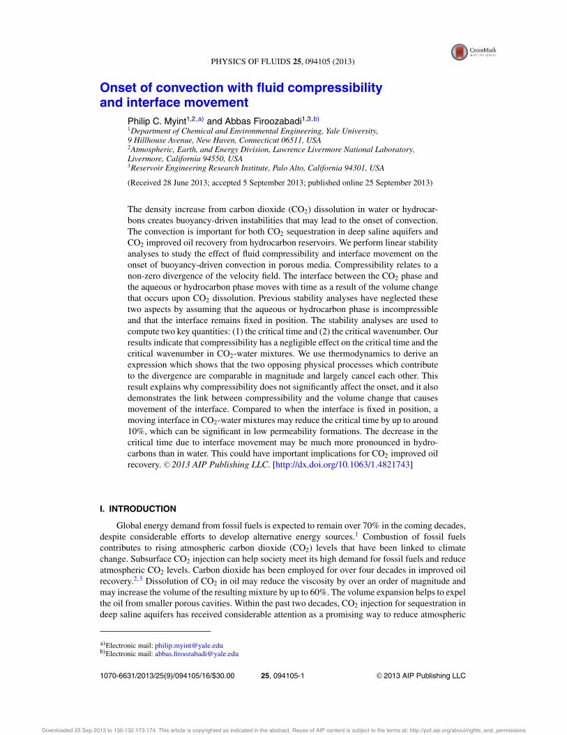
III. INTERFACE MOVEMENT

A. Governing and constitutive equations

Much of our formulation in Sec. III remains the same as in Sec. II. There are two importantdifferences, however: (1) we treat the liquid (aqueous or hydrocarbon) phase as being incompressible(# · q = 0), and (2) the position h(t) of the interface between the CO2 phase and the liquid phasemoves with time as a result of the volume change from CO2 dissolution. We consider a semi-infinitemedium where "' < z & h(t), with h(0) = 0. The velocity dh/dt with which the interface movescan be obtained from performing mass balances across the interface. The total mass balance andCO2 mass balance across the interface are,39–41 respectively,

!"G!

wGt " dh

dt

"= !"L

!wL

t " dhdt

", (45)

" !"G DG #cG

#z+ !cG"G

!wG

t " dhdt

"= "!"L DL #cL

#z+ !cL"L

!wL

t " dhdt

", (46)

where G denotes the CO2-rich side of the interface, L denotes the liquid side of the interface, and wt isthe true vertical velocity. This velocity is related to the Darcy vertical velocity w by wt = w/!. Thecomposition derivatives #cG/#z and #cL/#z are evaluated at the interface. We combine (45) and (46)to eliminate wG

t and obtain

wLt " dh

dt= " 1#

cG " cL$

!DL #cL

#z" "G

"LDG #cG

#z

".

If we use the fact that cG $ 1 throughout the entire CO2 phase because the solubility of liquid inCO2 is negligible (see Sec. I), the second term in the parentheses vanishes so that

dhdt

= wLt + DL

#1 " cL

$ #cL

#z. (47)

We approximate the convective velocity wLt as being zero because evaporation of liquid is negligible,

as stated in Secs. I and II C. Thus, (47) becomes

dhdt

= DL

#1 " cL

$ #cL

#z= D

(1 " csat)#c#z

,,,,z=h

. (48)

The governing equations in nondimensionalized form are given by (9), (10), and

# · q = 0, (49)

dhdt

= csat

(1 " csat)# c# z

,,,,z=h

, (50)



where h = h/&. The boundary conditions in z are

c(x, y, z = h, t) = 1, )x, y, t, (51)

w(x, y, z = h, t) = 0, )x, y, t, (52)

c(x, y, z ( "', t) = w(x, y, z ( "', t) = 0, )x, y, t . (53)

B. The base state

The base state concentration profile cbase(z, t) with a moving interface satisfies the one-dimensional diffusion equation (12), along with (50), the initial condition (13), the bottom boundarycondition (14), and the interface boundary condition

cbase(z = h, t) = 1, )t . (54)

The solution of this set of equations is analogous to the solution of the classical Stefan problem,which involves phase changes (e.g., melting of ice) that occur as a result of one-dimensional heatconduction.42 The moving interface in the Stefan problem represents the front where the phasechange occurs. The position h(t) of the interface in our problem indicates the extent of the volumechange; its value depends on the amount of CO2 dissolved in the liquid phase. The average CO2

concentration grows with the square root of time when the interface is fixed in position and the basestate is given by (16), as shown earlier.24, 43, 44 As an ansatz, we take h(t) to be proportional to thesquare root of time

h(t) = 2+*

t, (55)

where + is a dimensionless constant. The solution to (12)–(14) and (54)–(55) is

cbase(z, t) = 1 + erf(z/2*

t)1 + erf(+)

. (56)

The base state derivative with respect to z is

# cbase

# z= exp("z2/4t)

1 + erf(+)1*( t

. (57)

By substituting (55) and (57) into (50), we obtain a nonlinear equation

+[1 + erf(+)] exp(+2) = 1*(

csat

(1 " csat). (58)

For a given interfacial mass fraction csat, we must first solve (58) for +. This value of + can thenbe substituted into (55) to compute the interface position, into (56) to determine the concentrationfield, or into (57) to calculate the diffusive flux. In addition to (56), the base state is described by apressure field Pbase and qbase = 0.

C. Linearized perturbation equations

We follow the procedure described in Sec. II C and introduce perturbations to the base state,linearize the equations, and expand the perturbations using the Fourier transforms c+(s, z, t) andw+(s, z, t) to get

# c+

# t=

'"s2

%exp("z2/4t)1 + erf(+)

1*( t

&L"1 + L

*c+. (59)

We perform the non-modal stability analysis described in Sec. II C 2 to numerically integrate amatrix equation analogous to (38) using the same values of N, %z, %t , and the initial time. The only



difference is that after every time step, each grid point is moved a distance

dhdt

%t = +*t%t,

so that the topmost grid point is always located at z = h. As a result, we must add

dhdt

#

# z= +*

t

#

# z, (60)

to the matrix M to account for the movement of the mesh.

D. Results and discussion

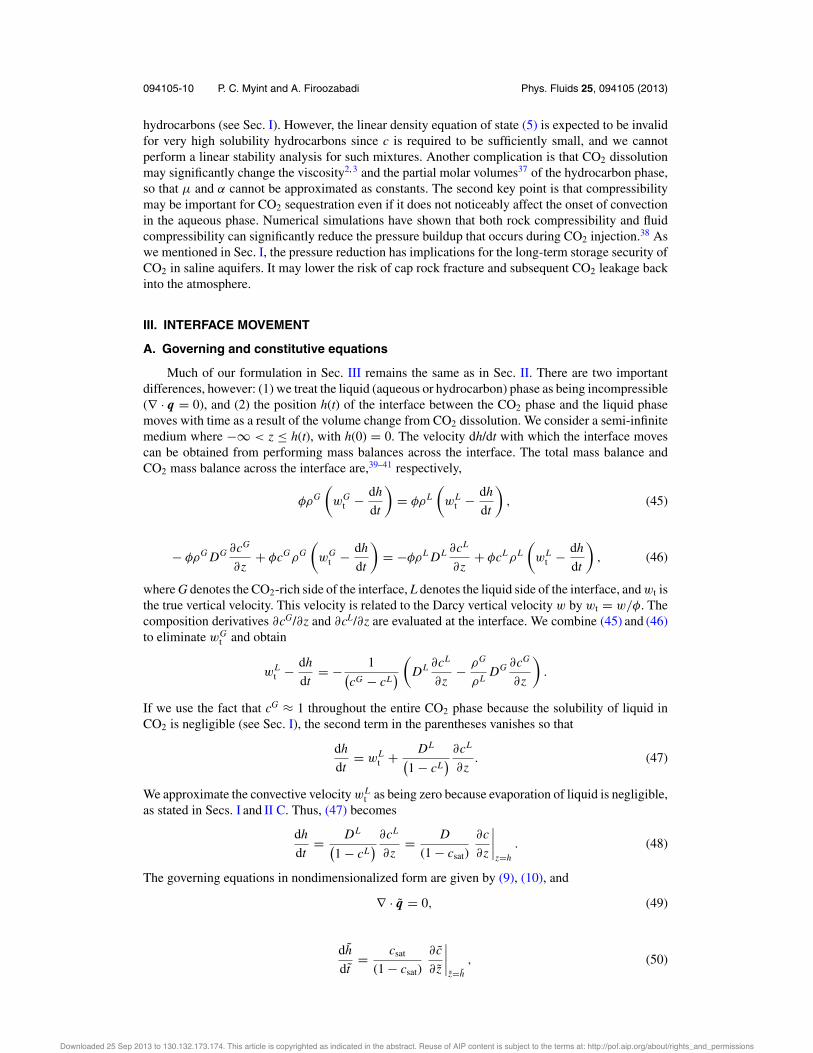
Figure 2 illustrates marginal stability contours of ) = 0 in wavenumber–time space.Equation (58) shows that the value of +, and therefore the extent of the volume change, depends oncsat. We present results for three different values of csat: 0.043, 0.08, and 0.12. The first is the samevalue used in Sec. II D. The second is the maximum solubility of CO2 in water at the conditionsexamined in our study. For comparison, we also present results for csat = 0.12, which could representa CO2-hydrocarbon mixture or a CO2-water mixture at pressures much higher than those consideredin our study.45, 46 In all cases, the effect of interface movement is much more prominent than theeffect of fluid compressibility. The contours are shifted downward and to the left with increasingvalues of csat, which indicates that interface movement decreases the critical time tc and the criticalwavenumber sc. Another way to quantify the effect of interface movement is to plot tc and sc as afunction of csat. This relationship is shown in Figure 3. Interface movement becomes negligible inthe limit as csat ( 0. The critical time and critical wavenumber approach the values of tc $ 50.2and sc $ 0.0666 from Sec. II D in this limit. We obtain the following scaling relations for thedimensionalized critical time tc and critical wavenumber sc from the best-fit lines:

tc = (50.2 " 66.4csat)' = (50.2 " 66.4csat)!

D1/2!µ

k%"g

"2

, (61)

sc = (0.0666 " 0.0192csat)/& = (0.0666 " 0.0192csat)!

k%"gD!µ

". (62)

These relations hold as long as csat is sufficiently small for (5) to be valid (see our discussion inSec. II A). We summarize our results in Table II, where “% difference” refers to the absolute percentdifference compared to the fixed interface. The decrease in tc in CO2-water mixtures can be up to

FIG. 2. (a) Marginal stability () = 0) contours in wavenumber–time space; (b) zoomed-in view around the critical time tcand the critical wavenumber sc. The moving interface shifts the contours downward and to the left, indicating a decrease inthe critical time and critical wavenumber. The effect becomes more pronounced for larger values of the interfacial CO2 massfraction csat.



0 0.05 0.1

(a) (b)

0.1540

42

44

46

48

50

52

csat (mass fraction)

t c(d

imen

sion

less

)

0 0.05 0.1 0.150.0635

0.064

0.0645

0.065

0.0655

0.066

0.0665

0.067

csat (mass fraction)

s c(d

imen

sion

less

)

FIG. 3. (a) and (b) The critical time tc and critical wavenumber sc for several values of the interfacial CO2 mass fractioncsat. Interface movement becomes negligible in the limit as csat ( 0. The best-fit lines represent tc = 50.2 " 66.4csat andsc = 0.0666 " 0.0192csat.

around 10% at the conditions examined in our study, but realistically not more than 20% even at veryhigh pressures. In contrast, Meulenbroek et al.34 have found that interface movement can lead tomore than a tenfold decrease in tc. They also model the time-dependence of h using (55). However,they determine + not from mass balances, but by examining the volume increase observed in PVTcell experiments where CO2 is mixed with oil or water.47 Determining + in this way may severelyoverestimate its magnitude because (55) is valid only before the onset of convection, yet the onsetis virtually instantaneous in these experiments so that much of the volume increase is due to theenhanced dissolution by convection. As a result, Meulenbroek et al.34 obtain a range for + between2 and 4, values that are roughly 100 times larger than our values. We expect the effect of interfacemovement to be much less pronounced than predicted by their analysis.

Nevertheless, since the time scale ' varies inversely with the square of the permeability k, a 10%reduction in tc can still be significant in low permeability media where ' is large. For a representativeset of conditions where D = 2 , 10"9 m2/s, ! = 0.2, µ = 0.001 Pa s, k = 0.1 darcy, and %"

= 10 kg/m3, we have ' $ 10 days. A 10% reduction in tc is equivalent to a decrease in the criticaltime tc of about 50 days for these conditions. If instead k = 0.01 darcy (it is not uncommon to findsuch low permeability formations), a 10% reduction in tc corresponds to a time period of about 5000days $ 13.5 years.

Movement of the interface affects the critical time in two opposing ways. Comparing(16) and (56), we see that the ratio of the concentration field cbase when the interface moves with

TABLE II. Summary of results in Figure 3. Interface movement may reduce tc in CO2-water mixtures by up to around 10%at the conditions examined in our study, but realistically not more than 20% even at very high pressures where the CO2solubility is relatively high.

+ tc % difference for tc sc % difference for sc

Fixed interface 0 50.2 . . . 0.0666 . . .csat = 0.02 0.0114 48.9 2.6 0.0663 0.5csat = 0.043 0.0246 47.4 5.6 0.0658 1.2csat = 0.06 0.0346 46.3 7.8 0.0655 1.7csat = 0.08 0.0465 44.9 10.6 0.0651 2.3csat = 0.10 0.0586 43.6 13.2 0.0647 2.9csat = 0.12 0.0709 42.3 15.7 0.0643 3.5csat = 0.14 0.0834 40.9 18.5 0.0638 4.2



time to cbase when the interface remains fixed is 1/[1 + erf(+)]. This ratio is less than one and mono-tonically decreases with + for + > 0. Thus, movement of the interface reduces the magnitude of cbase

because the increase in volume dilutes the CO2 concentration in the liquid phase. This translates toa reduction in the density " and an increase in the critical time. However, the volume expansion alsoincreases the thickness of the dense, CO2-dissolved liquid layer near the interface. The increasedthickness destabilizes the base state and allows the onset of convection to occur earlier. Previousstudies11, 16 have found that onset of convection cannot occur when the Rayleigh number Ra is lessthan about 30. Since Ra appears in location of the bottom boundary, this value of Ra represents theminimum height of the porous domain necessary for onset to occur. Slim and Ramakrishan16 reasonthat the vertical confinement when Ra < 30 impedes the growth of small wavenumber modes andprevents the formation of large-scale convection cells. We offer a different interpretation. We believethat Ra $ 30 represents a critical thickness of the CO2-dissolved liquid layer. When the thickness ofthe layer is less than this critical value (i.e., when only a small amount of CO2 has dissolved in theliquid phase), the buoyancy-driven instabilities are insufficiently strong to overcome the dissipationof the perturbations due to diffusion. The base state does not become unstable in such a case.

The onset of convection occurs earlier when the interface moves because the relative increasein the thickness is greater than the decrease in ". To show this, we examine the average mass density-"., which is the value obtained by spatially averaging " in all directions. It is equal to

-". = "0(1 + $-c.) = "0(1 + $-cbase.),

where the second equality follows from the fact that the perturbations do not affect the averageCO2 concentration. For illustration, we consider a binary mixture where csat = 0.08 and -". " "0

= 0.01"0. We have + = 0.0465 and 1/[1 + erf(+)] = 0.95 for this value of csat, and find that

-".moving

-".fixed= "0(1 + 0.0095)

"0(1 + 0.01)= 0.9995.

Interface movement decreases the average density by only 0.05%. Using the value of the Rayleighnumber from the preceding paragraph, the relative increase in the thickness of the CO2-dissolvedlayer may be estimated as h(tc)/30. For tc = 44.9, we have

h(44.9)30

= 2(0.0465)*

44.930

= 0.021.

Therefore, the relative increase in thickness may be over an order of magnitude greater than thedecrease in -".. In reality, the decrease in -". may be even less than the value calculated in ourexample. As mentioned in Sec. II A, the maximum density increase %" may be as high as about0.02"0 for CO2-water mixtures, and several percent of "0 for CO2-hydrocarbon mixtures. The onsetof convection occurs well before the liquid phase becomes saturated with CO2 at the equilibriumconcentration. Thus, -". " "0 % %", and the ratio -".moving/-".fixed will be closer to unity than inour example.

For the reasons discussed at the end of Sec. II D, we are unable to perform a stability analysisfor high CO2 solubility hydrocarbons where csat may be as large as 50 mass percent and swelling canbe as much as 60%. Nevertheless, the trends in our results strongly suggest that the decrease in thecritical time may be much more pronounced in hydrocarbons than in water. It may be comparableto the decrease in the critical time due to permeability anisotropy, which we have studied in ourprevious paper.24 This could have important implications for CO2 improved oil recovery.

IV. CONCLUSIONS

We have performed linear stability analyses to study the effect of fluid compressibility andinterface movement on the onset of buoyancy-driven convection in porous media. Our work has



applications to both CO2 improved oil recovery and CO2 sequestration, although we have focusedmainly on the latter. We draw the following conclusions:

! Compressibility, which is related to a non-zero divergence of the velocity field, has a negli-gible effect on the onset of convection in CO2-water mixtures. The critical time and criticalwavenumber for an incompressible vs. compressible fluid are virtually the same.! There are two contributions to the divergence of the velocity field: (1) a change in the volumeand (2) a change in the mass. The two contributions are comparable in magnitude for CO2-water mixtures and largely cancel each other. This explains why compressibility has a negligibleeffect, and it also suggests that the volume change from CO2 dissolution may be significant.The volume change is manifested in the form of a moving interface between the CO2 phaseand the liquid (aqueous or hydrocarbon) phase.! Interface movement may reduce the critical time by up to around 10% in CO2-water mixtures.The critical wavenumber also decreases, but to a lesser extent. A 10% reduction in the criticaltime can be significant in low permeability media, where it could represent a time period ofseveral months or even years.! The base state becomes more buoyantly unstable because interface movement increases thethickness of the dense, CO2-dissolved liquid layer near the interface. The end result is that theonset of convection occurs earlier.! The effect of a moving interface may be much more pronounced in hydrocarbons than in water.This could have important implications for CO2 improved oil recovery.

ACKNOWLEDGMENTS

Financial support for this work has been provided by the member companies of the ReservoirEngineering Research Institute.

1 “World energy outlook 2011,” Technical Report No. 61 2011 24 1P1, edited by F. Birol, L. Cozzi, A. Bromhead, J. Corben,M. Baroni, T. Gould, P. Olejarnik, D. Dorner, R. Priddle, and M. van der Hoeven (Directorate of Global Energy Economicsof the International Energy Agency, Paris, 2011).

2 A. Firoozabadi and P. Cheng, “Prospects for subsurface CO2 sequestration,” AIChE J. 56, 1398–1405 (2010).3 T. Ahmed, H. Nasrabadi, and A. Firoozabadi, “Complex flow and composition path in CO2 injection schemes from density

effects,” Energy Fuels 26, 4590–4598 (2012).4 G. J. Weir, S. P. White, and W. M. Kissling, “Reservoir storage and containment of greenhouse gases,” Transp. Porous

Med. 23, 37–60 (1996).5 E. Lindeberg and D. Wessel-Berg, “Vertical convection in an aquifer column under a gas cap of CO2,” Energy Convers.

Manage. 38, S229 (1997).6 “IPCC special report on carbon dioxide capture and storage,” Technical Report, edited by B. Mertz, O. Davidson, H. de

Doninck, M. Loos, and L. Meyer (Working Group III of the Intergovernmental Panel on Climate Change, CambridgeUniversity Press, Cambridge, 2005).

7 S. J. Ashcroft and M. Ben Isa, “Effect of dissolved gases on the densities of hydrocarbons,” J. Chem. Eng. Data 42,1244–1248 (1997).

8 J. Ennis-King and L. Paterson, “Role of convective mixing in the long-term storage of carbon dioxide in deep salineformations,” SPE J. 10, 349–356 (2005).

9 J. R. Johnston, “Weeks Island gravity stable CO2 pilot,” in Proceedings of the SPE Enhanced Oil Recovery Symposium,Tulsa, OK, USA, 1988 (The Society of Petroleum Engineers (SPE), 1988), p. 17351.

10 V. K. Bangia, F. F. Yau, and G. R. Hendricks, “Reservoir performance of a gravity-stable, vertical CO2 miscible flood:Wolfcamp Reef Reservoir, Wellman Unit,” SPE Reservoir Eng. 8, 261–269 (1993).

11 J. Ennis-King, I. Preston, and L. Paterson, “Onset of convection in anisotropic porous media subject to a rapid change inboundary conditions,” Phys. Fluids 17, 084107 (2005).

12 X. Xu, S. Chen, and D. Zhang, “Convective stability analysis of the long-term storage of carbon dioxide in deep salineaquifers,” Adv. Water Resour. 29, 397–407 (2006).

13 A. Riaz, M. Hesse, H. A. Tchelepi, and F. M. Orr, “Onset of convection in a gravitationally unstable diffusive boundarylayer in porous media,” J. Fluid Mech. 548, 87–111 (2006).

14 H. Hassanzadeh, M. Pooladi-Darvish, and D. W. Keith, “Stability of a fluid in a horizontal saturated porous layer: Effectof non-linear concentration profile, initial, and boundary conditions,” Transp. Porous Med. 65, 193–211 (2006).

15 S. Rapaka, S. Chen, R. J. Pawar, P. H. Stauffer, and D. Zhang, “Non-modal growth of perturbations in density-drivenconvection in porous media,” J. Fluid Mech. 609, 285–303 (2008).

16 A. C. Slim and T. S. Ramakrishan, “Onset and cessation of time-dependent, dissolution-driven convection in porous media,”Phys. Fluids 22, 124103 (2010).


http://dx.doi.org/10.1002/aic.12287

http://dx.doi.org/10.1021/ef300502f

http://dx.doi.org/10.1007/BF00145265

http://dx.doi.org/10.1007/BF00145265

http://dx.doi.org/10.1016/S0196-8904(96)00274-9

http://dx.doi.org/10.1016/S0196-8904(96)00274-9

http://dx.doi.org/10.1021/je9701588

http://dx.doi.org/10.2118/84344-PA


http://dx.doi.org/10.1063/1.2033911

http://dx.doi.org/10.1016/j.advwatres.2005.05.008

http://dx.doi.org/10.1017/S0022112005007494

http://dx.doi.org/10.1007/s11242-005-6088-1

http://dx.doi.org/10.1017/S0022112008002607

http://dx.doi.org/10.1063/1.3528009


17 H. Hassanzadeh, M. Pooladi-Darvish, and D. W. Keith, “The effect of natural flow of aquifers and associated dispersionon the onset of buoyancy-driven convection in a saturated porous medium,” AIChE J. 55, 475–485 (2009).

18 M. Javaheri, J. Abedi, and H. Hassanzadeh, “Linear stability analysis of double-diffusive convection in porous media, withapplication to geological storage of CO2,” Transp. Porous Med. 84, 441–456 (2010).

19 M. Bestehorn and A. Firoozabadi, “Effect of fluctuations on the onset of density-driven convection in porous media,” Phys.Fluids 24, 114102 (2012).

20 J. Ennis-King and L. Paterson, “Coupling of geochemical reactions and convective mixing in the long-term geologicalstorage of carbon dioxide,” Int. J. Greenhouse Gas Control 1, 86–93 (2007).

21 K. Ghesmat, H. Hassanzadeh, and J. Abedi, “The impact of geochemistry on convective mixing in a gravitationally unstablediffusive boundary layer in porous media: CO2 storage in saline aquifers,” J. Fluid Mech. 673, 480–512 (2011).

22 J. S. Hong and M. C. Kim, “Effect of anisotropy of porous media on the onset of buoyancy-driven convection,” Transp.Porous Med. 72, 241–253 (2008).

23 S. Rapaka, R. J. Pawar, P. H. Stauffer, D. Zhang, and S. Chen, “Onset of convection over a transient base-state in anisotropicand layered porous media,” J. Fluid Mech. 641, 227–244 (2009).

24 P. Cheng, M. Bestehorn, and A. Firoozabadi, “Effect of permeability anisotropy on buoyancy-driven flow for CO2sequestration in saline aquifers,” Water Resour. Res. 48, W09539, doi:10.1029/2012WR011939 (2012).

25 H. Hassanzadeh, M. Pooladi-Darvish, and D. W. Keith, “Scaling behavior of convective mixing, with application togeological storage of CO2,” AIChE J. 53, 1121–1131 (2007).

26 J. J. Hidalgo and J. Carrera, “Effect of dispersion on the onset of convection during CO2 sequestration,” J. Fluid Mech.640, 441–452 (2009).

27 G. S. H. Pau, J. B. Bell, K. Pruess, A. S. Almgren, M. J. Lijewski, and K. Zhang, “High-resolution simulation andcharacterization of density-driven flow in CO2 storage in saline aquifers,” Adv. Water Resour. 33, 443–455 (2010).

28 J. T. H. Andres and S. S. S. Cardoso, “Onset of convection in a porous medium in the presence of chemical reaction,”Phys. Rev. E 83, 046312 (2011).

29 M. T. Elenius and K. Johannsen, “On the time scales of nonlinear instability in miscible displacement porous media flow,”Comput. Geosci. 16, 901–911 (2012).

30 R. Farajzadeh, H. Salimi, P. L. J. Zitha, and H. Bruining, “Numerical simulation of density-driven natural convection inporous media with application for CO2 injection projects,” Int. J. Heat Mass Transfer 50, 5054–5064 (2007).

31 T. Kneafsey and K. Pruess, “Laboratory flow experiments for visualizing carbon dioxide-induced, density-driven brineconvection,” Transp. Porous Med. 82, 123–139 (2010).

32 R. Nazari Moghaddam, B. Rostami, P. Pourafshary, and Y. Fallahzadeh, “Quantification of density-driven natural convectionfor dissolution mechanism in CO2 sequestration,” Transp. Porous Med. 92, 439–456 (2012).

33 Z. Li and A. Firoozabadi, “Cubic-plus-association equation of state for water-containing mixtures: Is “cross association”necessary?” AIChE J. 55, 1803–1813 (2009).

34 B. Meulenbroek, R. Farajzadeh, and H. Bruining, “The effect of interface movement and viscosity variation on the stabilityof a diffusive interface between aqueous and gaseous CO2,” Phys. Fluids 25, 074103 (2013).

35 R. M. Lansangan and J. L. Smith, “Viscosity, density, and composition measurements of CO2/West Texas oil systems,”SPE Reservoir Eng. 8, 175–182 (1993).

36 T. D. Foster, “Stability of a homogeneous fluid cooled uniformly from above,” Phys. Fluids 8, 1249–1257 (1965).37 A. Firoozabadi, Thermodynamics of Hydrocarbon Reservoirs (McGraw-Hill, New York, 1999).38 J. Moortgat, Z. Li, and A. Firoozabadi, “Three-phase compositional modeling of CO2 injection by higher-order finite ele-

ment methods with CPA equation of state for aqueous phase,” Water Resour. Res. 48, W12511, doi:10.1029/2011WR011736(2012).

39 J. C. Slattery, Advanced Transport Phenomena (Cambridge University Press, Cambridge, 1999).40 L. G. Leal, Advanced Transport Phenomena: Fluid Mechanics and Convective Transport Processes (Cambridge University

Press, Cambridge, 2007).41 K. B. Haugen and A. Firoozabadi, “Composition at the interface between multicomponent non-equilibrium fluid phases,”

J. Chem. Phys. 130, 064707 (2009).42 J. Crank, Free and Moving Boundary Problems (Oxford University Press, Oxford, 1987).43 J. Crank, Mathematics of Diffusion, 2nd ed. (Oxford University Press, Oxford, 1980).44 H. S. Carslaw and J. C. Jaeger, Conduction of Heat in Solids, 2nd ed. (Oxford University Press, Oxford, 1986).45 S. Takenouchi and G. C. Kennedy, “The binary system H2O-CO2 at high temperatures and pressures,” Am. J. Sci. 262,

1055–1074 (1964).46 A. E. Mather and E. U. Franck, “Phase equilibria in the system carbon dioxide-water at elevated pressures,” J. Phys. Chem.

96, 6–8 (1992).47 R. Farajzadeh, H. A. Delil, P. L. J. Zitha, and J. Bruining, “Enhanced mass transfer of CO2 into water and oil by natural

convection,” in Proceedings of the SPE Europec/EAGE Annual Conference and Exhibition, London, UK, 2007 (The Societyof Petroleum Engineers (SPE), 2007), p. 107380.



http://dx.doi.org/10.1007/s11242-009-9513-z

http://dx.doi.org/10.1063/1.4767467

http://dx.doi.org/10.1063/1.4767467

http://dx.doi.org/10.1016/S1750-5836(07)00034-5

http://dx.doi.org/10.1017/S0022112010006282

http://dx.doi.org/10.1007/s11242-007-9147-y

http://dx.doi.org/10.1007/s11242-007-9147-y

http://dx.doi.org/10.1017/S0022112009991479

http://dx.doi.org/10.1029/2012WR011939


http://dx.doi.org/10.1017/S0022112009991480

http://dx.doi.org/10.1016/j.advwatres.2010.01.009

http://dx.doi.org/10.1103/PhysRevE.83.046312

http://dx.doi.org/10.1007/s10596-012-9294-2

http://dx.doi.org/10.1016/j.ijheatmasstransfer.2007.08.019

http://dx.doi.org/10.1007/s11242-009-9482-2

http://dx.doi.org/10.1007/s11242-011-9911-x


http://dx.doi.org/10.1063/1.4813072


http://dx.doi.org/10.1063/1.1761393

http://dx.doi.org/10.1029/2011WR011736

http://dx.doi.org/10.1063/1.3072793

http://dx.doi.org/10.2475/ajs.262.9.1055

http://dx.doi.org/10.1021/j100180a003

Documents

Onset of convection with ﬂuid compressibility and ... Pub/MyintFiroozabadiPoF2013a.pdf · PHYSICS OF FLUIDS25,094105(2013) Onset of convection with ﬂuid compressibility and interface