Embed Size (px)
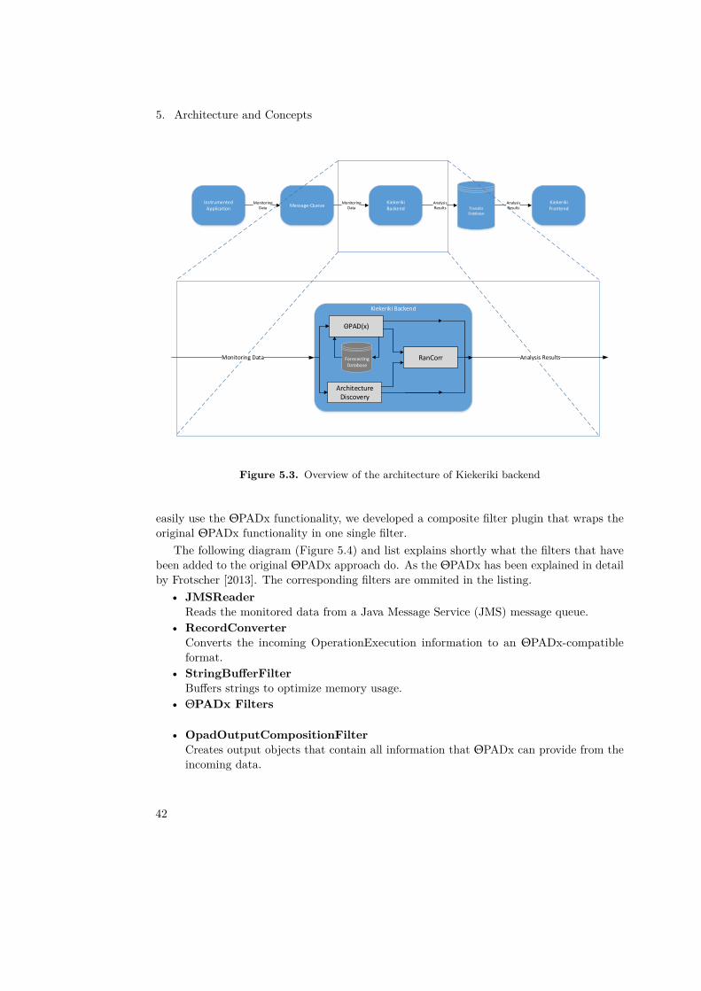
Citation preview
Institute of Software Technology
University of StuttgartUniversitätsstraße 38
D–70569 Stuttgart
Development Project
Online Performance ProblemDetection, Diagnosis, andVisualization with Kieker
T. Düllmann, A. Eberlein, C. Endres, M. Fetzer, M.Fischer, C. Gregorian, K. Képes, Y. Noller, D. Olp, T.
Rudolph, A. Scherer, M. Scholz
Course of Study: Software Engineering
Examiner: Prof. Dr. Lars Grunske
Supervisor: Dipl.-Inform. André van Hoorn
Commenced: 2013/11/18
Completed: 2014/03/31
CR-Classification: H.3.4, H.5.2

Abstract
With increasingly large systems Online Performance Monitoring becomes more and morea necessity to find, predict, and recover from failures. The Kieker monitoring tool enablesthe monitoring and analysis of applications. It allows to gather live data about the systemsutilization like RAM-load, Swap-load, CPU-load as well as the latency of executed operationsand their qualified name. ΘPADx provides means to detect anomalous behaviour andRanCorr allows the correlation of anomalies to identifiy the root cause of an anomaly. Thisproject implements the RanCorr approach and extends the ΘPAD implementation withnew forecast algorithms. Also the Kieker-WebGUI is extended to visualize the architecture,discovered by RanCorr, and other metrics by using dynamic diagrams. Additionally, anautomated test framework is introduced that enables data generation and evaluation of theimplemented forecasting and anomaly detection approach.
3


Contents
1 Introduction 11.1 Motivation and Goals . . . . . . . . . . . . . . . . . . . . . . . . . . . . . . . 11.2 Document Structure . . . . . . . . . . . . . . . . . . . . . . . . . . . . . . . . 2
2 Foundations and Technologies 32.1 ΘPAD and RanCorr . . . . . . . . . . . . . . . . . . . . . . . . . . . . . . . . 32.2 CoCoME . . . . . . . . . . . . . . . . . . . . . . . . . . . . . . . . . . . . . . 52.3 Kieker and Kieker WebGUI . . . . . . . . . . . . . . . . . . . . . . . . . . . . 62.4 APM Tools . . . . . . . . . . . . . . . . . . . . . . . . . . . . . . . . . . . . . 72.5 Failure Diagnosis . . . . . . . . . . . . . . . . . . . . . . . . . . . . . . . . . . 82.6 Design of Performance Experiments . . . . . . . . . . . . . . . . . . . . . . . 92.7 Trashing JPetStore . . . . . . . . . . . . . . . . . . . . . . . . . . . . . . . . . 92.8 Tooling . . . . . . . . . . . . . . . . . . . . . . . . . . . . . . . . . . . . . . . 10
3 Requirements 153.1 Frontend Requirements . . . . . . . . . . . . . . . . . . . . . . . . . . . . . . 153.2 Backend . . . . . . . . . . . . . . . . . . . . . . . . . . . . . . . . . . . . . . . 183.3 Interface . . . . . . . . . . . . . . . . . . . . . . . . . . . . . . . . . . . . . . . 21
4 Project Management 234.1 Tooling . . . . . . . . . . . . . . . . . . . . . . . . . . . . . . . . . . . . . . . 234.2 Scrum . . . . . . . . . . . . . . . . . . . . . . . . . . . . . . . . . . . . . . . . 294.3 Team . . . . . . . . . . . . . . . . . . . . . . . . . . . . . . . . . . . . . . . . . 344.4 Roles . . . . . . . . . . . . . . . . . . . . . . . . . . . . . . . . . . . . . . . . . 37
5 Architecture and Concepts 395.1 Overview . . . . . . . . . . . . . . . . . . . . . . . . . . . . . . . . . . . . . . 395.2 Frontend . . . . . . . . . . . . . . . . . . . . . . . . . . . . . . . . . . . . . . . 395.3 Backend . . . . . . . . . . . . . . . . . . . . . . . . . . . . . . . . . . . . . . . 415.4 Raw Data, Data Aggregation and Metrics . . . . . . . . . . . . . . . . . . . . 46
6 Current state 536.1 Kieker Backend . . . . . . . . . . . . . . . . . . . . . . . . . . . . . . . . . . . 536.2 Kieker Frontend . . . . . . . . . . . . . . . . . . . . . . . . . . . . . . . . . . 54
5
Contents
7 Implementation 577.1 Backend . . . . . . . . . . . . . . . . . . . . . . . . . . . . . . . . . . . . . . . 577.2 Frontend . . . . . . . . . . . . . . . . . . . . . . . . . . . . . . . . . . . . . . . 697.3 Transfer Database . . . . . . . . . . . . . . . . . . . . . . . . . . . . . . . . . 787.4 Transfer Database Data Generator and Benchmarking Tool . . . . . . . . . . 81
8 Experiments and Validation 838.1 Experiments and validation of the Kiekeriki Backend . . . . . . . . . . . . . . 838.2 Benchmarks of the Database Connections . . . . . . . . . . . . . . . . . . . . 1208.3 Usability Study of the WebGUI conducted with APM-Experts . . . . . . . . 130
9 Future Work 1379.1 Backend . . . . . . . . . . . . . . . . . . . . . . . . . . . . . . . . . . . . . . . 1379.2 Frontend . . . . . . . . . . . . . . . . . . . . . . . . . . . . . . . . . . . . . . . 138
Bibliography 141
6
Chapter 1
Introduction
1.1 Motivation and Goals
Our motivation for this project lies within not only expanding the functionality of Kieker,but also in the visualization of data. Huge amounts of data are of little use if they cannotbe seen and rapidly evaluated by a human. Therefore it is important to prepare our datato allow ease of access and analysis for the GUI, as well as formatting said GUI to displaythe most vital information in an easy to understand manner. As mentioned, we also wishto expand the functionality of Kieker by implementing a new plugin to allow a better liveanalysis of running systems that allows not only detecting errors, but also delivering accuratedata for solving issues.
• Goal 1: Expand Kieker Functionality– Goal 1a: Extend ΘPADx implementation by adding a Self-Tuning Algorithm.
While ΘPAD is functional, it lacks the ability to change its parameters at runtime,an important step for implementing adaptability in any algorithm. It is necessaryto implement both the ability to allow the values to be changed as well as thelearning algorithms that control the variables containing those values.
– Goal 1b: Create Plugin using the RanCorr algorithm provided.In order to further understanding of the data created by Kieker, RanCorr willbe implemented leading to a correlation between anomalies and the structuresin which those anomalies occur. The root cause analysis is a useful tool forsystem analysis, cutting search times by pointing out culprits in case of errors orslowdowns.
– Goal 1c: Validate both ΘPADx and RanCorr outputs. Simply implementingself-tuning ΘPADx and RanCorr is not sufficient. In order to verify the changes itis necessary to take measurements considering the actual accuracy of the changesversus the results they delivered beforehand.
• Goal 2: Create Frontend to display gathered data in a useful manner– Goal 2a: Get rid of the Pipes and Filter view to set up the monitoring and create
a simpler way for the specific purpose addressed in this project while keeping allpossibilities to configure the backend.
– Goal 2b: Show the architecture of the monitored system and offer the possibilityto examine the components of the system using a deep dive approach.
1
1. Introduction
– Goal 2c: Offer the possibility to create dynamically new diagrams. This willreplace the old cockpit view to show the data of the different metrics.
Christopher Gregorian and Martin Scholz
1.2 Document StructureThis document continues with Chapter 2 which presents the foundations gained in theseminar talks. The Chapter 3 describes the requirements for frontend, backend and theinterface between them. Then the Chapter 4 shows how the project was organized andthe technical support. Section 4.3 provides the task distribution across the team members.Afterwards Section 4.4 presents the different organizational roles which were defined in theproject. Then Chapter 5 shows the overall architecture designed in this project. Chapter 6describes the current state before the project started. The Chapter 7 continues with thedescription about the actual implementation work. Afterwards the Chapter 8 provides thevalidation description and interpretation. Finally Chapter 9 shows the possible future workwhich could be done in order to extend this project.
Yannic Noller
2
Chapter 2
Foundations and Technologies
2.1 ΘPAD and RanCorrAs described in chapter 1.1 this project aims to extend the ΘPAD approach among othersby implementing the idea of RanCorr. Therefore it’s necessary to understand the basics ofanomaly detection and especially the ideas of ΘPAD and RanCorr.
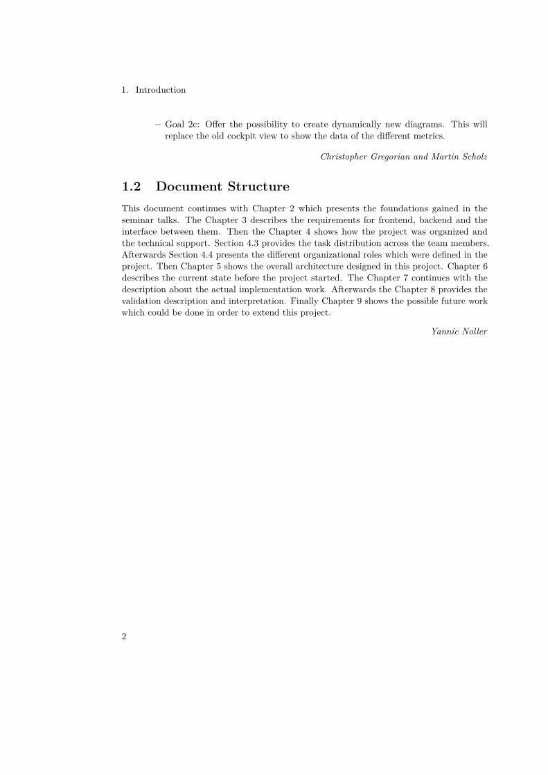
2.1.1 Online Performance Anomaly Detection (ΘPAD)The ΘPAD approach was introduced in the diploma thesis by Bielefeld [2012] and meansOnline Performance Anomaly Detection. Frotscher [2013] extended the ΘPAD approach inhis master thesis and named it ΘPADx. In this document we still talk about the ΘPADapproach, but mean the latest version. ΘPAD detects anomalies in performance data basedon discrete time series analysis. It’s divided in five steps like shown in Figure 2.1 suitable forKieker’s Pipes-and-Filter architecture.
Reader Time SeriesForecasting
Anomaly ScoreCalculation
Time SeriesExtraction
AnomalyDetection Alerting
Figure 2.1. Analysis steps of ΘPAD approach based on Bielefeld [2012] consisting of: (1) readingof measurement data, (2) extraction of discrete time series, (3) forecasting of next observation basedon historical data, (4) calculation of anomaly score based on difference between observations andforetold reference model, (5) detection of anomaly based on anomaly score threshold and (6) alertingin case of an anomaly.
The first step Reader reads the input data of ΘPAD which are the raw measurements of aperformance metric like response time in continuous time series. The second step Time SeriesExtraction converts the continuous time series in a discrete one by aggregating the data indiscrete time periods. For the aggregation a simple unweighted arithmetic mean functioncould be used. The third step Time Series Forecasting calculates a forecasting value for thenext time period. ΘPAD supports multiple forecasting methods. The simplest one is calledMoving Average which calculates the unweighted arithmetic mean of a sliding time windowas forecasting value. More methods are ARIMA or Single Exponential Smoothing (SES). The
3
2. Foundations and Technologies
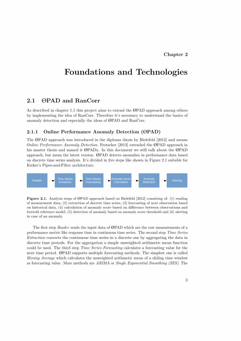
fourth step Anomaly Score Calculation uses the forecasting values of the previous step asreference model in order to compare it with the actual observations. The difference valueis mapped to range between 0 and 1 and is called anomaly score. The fifth step AnomalyDetection uses a predefined anomaly threshold to detect an anomaly: if the anomaly scoreexceeds the threshold, the measured values will be considered as an anomaly. The last stepAlerting can be used to notify e.g. an administrator about the detected anomaly. ΘPADworks fine for point anomalies and contextual anomalies, but for collective anomalies (seeFigure 2.2) the reference model contains to much mutated values and the system generatesfalse positive results. This can lead to frustrated users and bad user acceptance. ThereforeFrotscher [2013] introduced with ΘPADx a new forecasting method called Pattern Checkingwhich searches in case of collective anomalies a better reference model in the historical data.However, the ΘPAD approach provides only the detection of anomalies and not a root causeanalysis of them. This needs a correlation of anomaly scores like described in the nextsection.
5 10 15
5
10
pointanomaly
contextualanomaly
collectiveanomaly
Figure 2.2. Overview about the three anomaly types: point, contextual and collective anomalies(based on Frotscher [2013]).
2.1.2 Anomaly Correlation: RanCorr
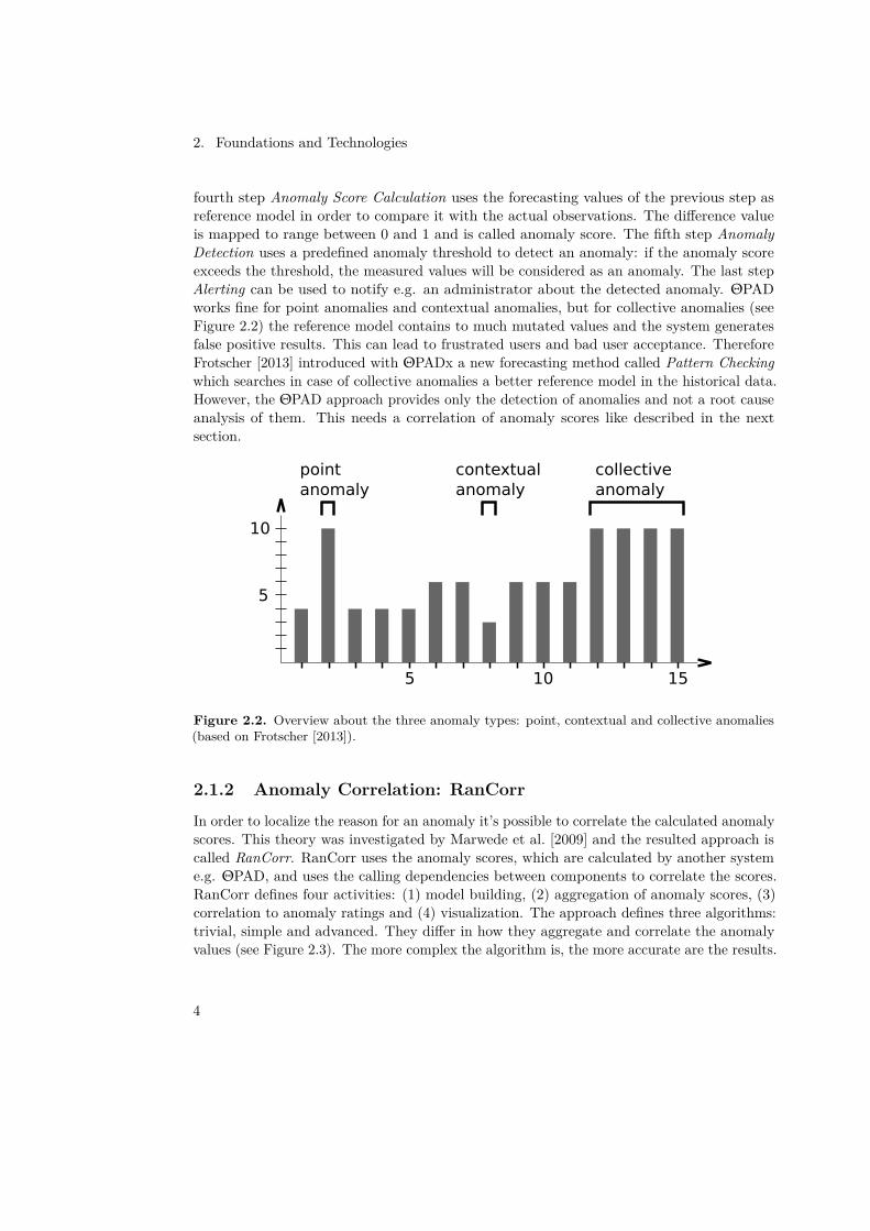
In order to localize the reason for an anomaly it’s possible to correlate the calculated anomalyscores. This theory was investigated by Marwede et al. [2009] and the resulted approach iscalled RanCorr. RanCorr uses the anomaly scores, which are calculated by another systeme.g. ΘPAD, and uses the calling dependencies between components to correlate the scores.RanCorr defines four activities: (1) model building, (2) aggregation of anomaly scores, (3)correlation to anomaly ratings and (4) visualization. The approach defines three algorithms:trivial, simple and advanced. They differ in how they aggregate and correlate the anomalyvalues (see Figure 2.3). The more complex the algorithm is, the more accurate are the results.
4
2.2. CoCoME
Appeared in A. Winter, R. Ferenc, and J. Knodel (eds.), Proceedings of the 13th EuropeanConference on Software Maintenance and Reengineering (CSMR 2009), pages 47–57. IEEE.March 2009.
4
Co
mp
on
en
t
Le
ve
l
unweighted
arithmetic mean
Op
era
tion
Le
ve
l
De
pl. C
on
t.
Le
ve
l
unweighted
arithmetic mean
unweighted
arithmetic mean
Aggregation
Aggregation
Aggregation
Correlation
unweighted
arithmetic mean
unweighted
arithmetic mean
unweighted
arithmetic mean
unweighted
arithmetic mean
unweighted
power mean
unweighted
power mean
unweighted
power mean
distance and call freq.
weighted power mean
Trivial Simple Advanced
Figure 4. Three algorithm variants deriveanomaly ratings from anomaly scores pro-vided by an anomaly detector. Anomaly rat-ings are computed for operations, compo-nents, and deployment contexts.
effects. The advanced algorithm uses enhanced aggregationand correlation methods to consider more assumptions onhow propagation effects distribute anomaly scores amongthe components.
4.1 Trivial Algorithm
The trivial algorithm aggregates anomaly scores s ∈ Si todetermine the anomaly rating ri of an operation i (the i-thoperation provided by the anomaly detector). The aggre-gation uses the unweighted arithmetic mean as shown inEquation 1.
ri := Si :=1|Si| ·
∑s∈Si
s (1)
As displayed in Figure 4, the unweighted arithmetic meanis also used to aggregate a component’s anomaly rating, anda deployment context’s rating from the corresponding oper-ation ratings and component ratings respectively.
4.2 Simple Algorithm
Two rules are used to detect configurations in the anomalystructure that are relatively clear to understand and to imple-ment. Two specific conditions are tested, and an increase ordecrease flag is set. Additional information is completely
ignored, because its effects are unknown and could be mis-leading. The cause rating is then derived from the anomalyrating, according to the flags.
More precisely, the anomaly rating is increased if the un-weighted arithmetic mean of the anomaly ratings of the di-rectly connected callers (upwards in the calling dependencygraph) is greater than the anomaly rating of the currentlyconsidered operation. This means that this operation islikely to be the cause of failure, because the dependent oper-ations show significant anomalies. The rating is decreasedif the maximum of the anomaly ratings of the directly con-nected callees (downwards in the graph) is greater than theanomaly rating of the current operation. This means thatthis operation’s rating is likely to be a propagation from an-other operation it depends on. Under all other conditions,as well as in special cases such as singular connections, andthe root operation, the value of the anomaly rating is for-warded without change.
Equation 2 defines the correlation function of the simplealgorithm that computes ri as the anomaly rating for op-eration i, Si as the (unweighted arithmetic) mean anomalyscore for operation i, S
in
i as the mean of all anomaly scorescorresponding to operations with calls to i, and maxout
i asmax{Sk|k is operation called by operation i}.
ri :=
12 · (Si + 1), S
in
i > Si ∧ maxouti ≤ Si
12 · (Si − 1), S
in
i ≤ Si ∧ maxouti > Si
Si, else
(2)
The function for increase and decrease ( 12 · (Si ± 1)) is
chosen for its simple linear graph, staying in range [−1, 1].Again, the aggregation is done through an unweighted arith-metic mean calculation on all three levels.
4.3 Advanced Algorithm
The advanced algorithm extends the simple algorithm bythe following features:
• The anomaly rating for each node is computed by ag-gregating the anomaly scores of its forward and back-ward transitive closure. For instance, the anomaly rat-ing for the nodeD (Figure 5) is computed based on theaggregated anomaly scores (values inside the nodes) ofA, B, H–J, F, and G, in contrast to the simple algorithmthat considers only A, B, F, and G.
• Distance and edge weights, i.e., the calling frequen-cies, are used to weight the connections. Togetherwith the consideration of the transitive closure de-scribed above, this models the observation that anoma-lies propagate via the edges over the complete callinggraph with descending strength by increasing distance.
Figure 2.3. Aggregation and correlation steps of RanCorr shown for every algorithm (trivial,simple and advanced) based on Marwede et al. [2009]. The first row shows the aggregation functionfor the local anomaly scores of an operation. In case of the trivial algorithm this aggregated anomalyscore is already the anomaly ranking, but in case of the simple and the advanced algorithm there isan additional correlation step between the dependencies of the considered operation. Afterwards theanomaly ranking will be aggregated for all hierarchy levels.
Yannic Noller
2.2 CoCoMEIn order to create real application data, we took several Common Component ModelingExample (CoCoME) [Herold et al., 2008] implementations into consideration. It is a realworld application example used for many different purposes in research. CoCoME is a modelof a supermarket trading system that consists of several modules (e.g. enterprise, inventory,store, cashdesk, bank) which interact with each other. CoCoME is modeled to be able to actas a distributed system, which would be useful for testing purposes.
To evaluate whether a CoCoME implementation could be useful for our testing and datageneration purposes we obtained several implementations. We tried to use the CoCoME CoC[b] implementation to serve as data generation application which provided multiple GraphicalUser Interfaces (GUIs) to control the example (e.g. inventory lists, cashdesk process).
Unfortunately it was not possible to get the other implementations (CoCoME2 CoC [a],SOFA Shop Sof) to run. Due to tool or package requirements and quite small manuals wecould not start them properly. This might also be caused by the specific implementation ofthe applications as different research groups use CoCoME for different purposes:
5
2. Foundations and Technologies
• monitoring and reverse engineering tools (e.g. Kieker Jung et al. [2013])• Cloud Computing/Service Oriented Architecture (SOA) Jung et al. [2013]; Hasselbring
et al. [2013]• Model Driven Engineering• etc.The main problem was that the documentation of how to set the implementations up
and how to use them was quite small. Therefor sometimes it was not clear how to usethe applications correctly. Due to the relatively high effort that would have to be madeto understand the workflows within those implementations we decided not to use CoCoMEimplementations for test data generation.
Thomas Düllmann
2.3 Kieker and Kieker WebGUI
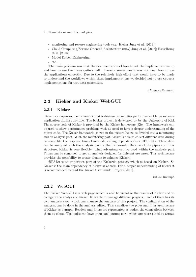
2.3.1 KiekerKieker is an open source framework that is designed to monitor performance of large softwareapplication during run-time. The Kieker project is developed by by the University of Kiel.The source code of Kieker is provided by the Kieker homepage [Kie]. The framework canbe used to show performance problems with no need to have a deeper understanding of thesource code. The Kieker framework, shown in the picture below, is divided into a monitoringand an analysis part. With the monitoring part Kieker is able to collect different data duringrun-time like the response time of methods, calling dependencies or CPU data. These datacan be analyzed with the analysis part of the framework. Because of the pipes and filterstructure, Kieker is very flexible. That advantage can be used within the analysis part.Filters can be combined to get an analysis designed for different use cases. This architectureprovides the possibility to create plugins to enhance Kieker.
ΘPADx is an important part of the Kiekeriki project, which is based on Kieker. SoKieker is the main dependency of Kiekeriki as well. For a deeper understanding of Kieker itis recommended to read the Kieker User Guide [Project, 2013].
Tobias Rudolph
2.3.2 WebGUIThe Kieker WebGUI is a web page which is able to visualize the results of Kieker and toconfigure the analysis of Kieker. It is able to manage different projects. Each of them has itsown analysis view, which can manage the analysis of this project. The configuration of theanalysis, can be done in the analysis editor. This visualizes the pipes and filter architectureof Kieker as a graph. Readers and filters are represented as nodes, the connections betweenthem by edges. The nodes can have input- and output ports which are represented by arrows
6
2.4. APM Tools
Figure 2.4. Overview of the architecture of Kieker
on the nodes. It is possible to create new edges between the readers and filters. In this way,new analyses can be created.
Another view is the cockpit view. In this page, several metrics are shown using differentkinds of diagrams. The diagrams use the data gathered by the analysis. The cockpit view canbe configured, too. It is possible to place different diagrams on the cockpit view, dependingon which metrics are gathered.
The Kieker WebGUI uses PrimeFaces for displaying the content. It runs best on a jettywebserver. The WebGUI can be downloaded on the kieker homepage as executable binaryfile or as eclipse/netbeans project. Several example projects are included. See chapter X forthe architecture of the WebGUI.
2.4 APM ToolsApplication Performance Management(also kown as Application Performance Monitoring)crosses a wide range of IT disciplines in order to detect, prioritize and resolve performanceand availability problems that affect business applications (Shields [2010]). A low overheadproduction and diagnosis capabilities are essential. Gartner defined the five dimensions enduser experience, runtime application architecture, business transactions, deep dive componentmonitoring and analysis/reporting for evaluating the APM tool market. He revealed that in2013, the best commercial vendor was AppDynamics. Some features of this tool which canbe relevant to our project are described in the following. First, the deep dive approach intocomponents is helpful to get from a high level view into a detailed view (e.g. on method level).This enables multiple troubleshooting mechanisms. Next, end user monitoring which analyzes
7
2. Foundations and Technologies
how end users perceive the actual performance is an approach which gains importance overthe last years. However, it will not be implemented in this project. Defining health rules forservers or business transactions gives a good overall view of the monitored system. Therefore,similar features could be relevant for our project. Then, alert and respond features after ananomaly or an exception occurred are important in production mode, e.g. for sending ane-Mail to responsible persons. To limit the tasks for this project, this will not be part ofthe product backlog. Finally, business transactions are fundamental for APM tools as theyreveal important information about the business impact of user requests. Detecting businesstransactions and showing them shall be part of the upcoming work. Showing live data in theGUI is feauture, all important APM tools are capable of.
Anton Scherer
2.5 Failure DiagnosisModern computer systems are getting larger and more complex over time due to frequentupdates, repairs or through new components getting integrated and other components gettingseparated. To prevent system failures or limit the potential damage caused by system failureswe try to predict if failures are about to happen in the near future and induce necessarysteps to prevent them or recover fast. This section is a brief summary of Salfner et al. [2010].
2.5.1 Proactive Fault ManagementThe term ”Proactive Fault Management” describes a technique to cope with occuring failures.The main motivation is, that a system is made aware of upcoming failures and can theninduce actions to prevent failures from happening or to prepare measures for a fast recovery.Proactive Fault Management consists of four basic steps:
1. Online Failure Prediction tries to identify situations that have a high probability thata failure is about to happen. The result of Online Failure Prediction can be binary decisionor another measure. E.g. ”There is a 70% probability that a failure will occure within thenext 5 minutes”.
2. Diagnosis is the task of finding out, what exactly is about to happen. It may be relevantto know where the failure is located and what exactly the failure is. E.g. ”That serverwill go offline because its database is flooded”.
3. Action Scheduling tries to determine what actions have to be executed to best resolvethe current situation. The decision is based on the outcome of the Online Failure Predictionas well as the Diagnosis. Relevant factors in the decision process are the cost of action,confidence in the prediction, and effectiveness and complexity of the actions. E.g. a highcost action will only be executed when failure occurence is almost certain.
4. Execution of Actions is the last step in Proactive Fault Management.
8

2.6. Design of Performance Experiments
2.5.2 Definitions• A failure is ”an event that occurs when the delivered service deviates from the correct
service”. A failure can be observed by any party that uses a system. There is no failureas long as the output is as specified.
• An error occurs when the current system state differs from the correct system state.An error may lead to a system failure.
• A fault is the cause of an error. Faults can be existing dormant in a system. Theiractivation causes an incorrect system state.
• Errors can be further classified in undetected and detected errors. Undetected errorsbecome detected errors when an incorrect system state is identified.
• Undetected or detected errors may not only be the cause of failures but also of symptoms.A symptom is an out-of-norm behaviour of system parameters caused by errors.
2.5.3 Online PredictionOnline Prediction is the task of predicting the potential of failure occurrence for a time inthe future (lead time) based on the current state of the system. The system state is assesedthrough monitoring within a window of certain length. Any prediction is only valid for acertain amount of time (prediction period).Increasing the prediction period results in increased probability that a failure is predictedcorrectly. But if the increased prediction period is too long, the information becomes irrelevantdue to its inaccuracy.A leadtime that is larger than the systems reaction time to avoid a failure, is not very sensible.Therefore a minimal warning time is introduced. If the lead time is shorter than the minimalwarning time, there is not sufficient time for the system to react to a upcoming failure.
Markus Fischer
2.6 Design of Performance Experiments
2.7 Trashing JPetStoreWhile Kieker currently collects several metrics (including but not limited to CPU usage,Memory and Latency), we are concentrating on the Latency of individual function calls. Datagathered via this metric is analyzed byΘPADx and RanCorr implementations for anomalies,which is then forwarded to the GUI.
Both our Front- and Back-end will allow automatic testing of their features. In the caseof the Back-end, this will include Input Generation, Input Manipulation, Anomaly Insertionand automated evaluation of the results delivered. By creating automated testing tools, it ispossible to support rapid development not only by our team, but by future users of our work.
9
2. Foundations and Technologies
In this section we give an introduction on JPetStore and some applications of ApacheJMeter Plans. JPetStore was originally a release and demo by Sun, which was showcase ofJava BestPractices and JavaEE. With the time is became also one reference application forJavaEE. With the time vendors like Mircosoft their own versions of the PetStore using the.NET Framework. As the requirements of both reference applications were similar, someperformance comparisons between the Java and .NET worlds were made. Another versionof JPetStore is available, MyBatis released their own version of the store. MyBatis is aframework that allows decoupling of database statements from the code, atop of this theMyBatis version is build using the Spring Framework, a Model-View-Controller frameworkwith the same goal as Java EE and additionaly the Stripes framework is used for MVC WebApplications.
The general access and usage of the MyBatis JPetStore is based on a HTTP API consistingout of multiple resources.
• The catalog is the main resource for the pets in the store– http://localhost:8080/jpetstore/actions/Catalog.action
• The following queries for example allow requests for the pet information pages– ?viewCategory=&categoryId=FISH, will show all pets that are fish in the store– ?viewProduct=&productId=FI-FW-01, would should a undercategory of a kind of animals– ?viewItem=&itemId=EST-4, itemId is used for a single entity of animal
• Adding and removing animals from the cart is done by the following URI’s:– /jpetstore/actions/Cart.action?removeItemFromCart=&cartItem=EST-6
– /jpetstore/actions/Cart.action?addItemToCart=&workingItemId=EST-26
To generate data with the JPetStore that represent anomalies Apache JMeter was used.JMeter is a tool which can be used for performance and load testing purposes. For that,JMeter allows to define threads in a Test Plan, where a single thread can have an assignedplan of steps it should execute. The steps can include SOAP, HTTP and FTP requests ordatabase statements. The general concept was to verify whether JPetStore was suitable touse for anomaly checking with the metrics that had to be implemented by the developmentteam. The results where enough for anomaly detection. With 100.000 requests on the sameresource of the store, anomalies with deviatons of 5.400 milliseconds where possible, which isenough for testing purposes.
2.8 ToolingAgile software development such as Scrum is facilitated by choosing and using the right tools.These allow programmers and project managers to work independently and transparently byutilizing a central maintenance.
The distribution of tasks to individual or multiple programmers for example, is donevia an issue tracking system (ITS). Using ITS, all participants in the project can both
10

2.8. Tooling
manage tasks and plan the project schedule. This includes the sprint planning, the schedulingof milestones or the classification of the development process in developing steps. Likewise,working time and effort are documented.
Encountered errors must be recorded when testing the software components or usingcode parts of other software developers. In this way the risk of losing sight of the error incomplex software drastically decreases. This is simplified if a Bug tracking system (BTS)is used, which ideally is closely linked to the ITS. The responsible developer may makeobservations in the BTS or request additional details that are needed to reproduce the error.
Issue tracking systems and bug tracking systems primarily serve the organization ofthe development project, but are not directly related to the program code. In order tofacilitate concurrent and efficient work of several developers, a software version controlsystem (VCS) can be used. A VCS manages the program code centrally and recognizes allthe innovations and changes that the developers made.
Andreas Eberlein
2.8.1 Version Control SystemA version control system (VCS) is a system that tracks all changes to a file or folder whichis under version control. Developers can retrieve the current state of the software theyare working on and submit their local changes to the version control system. This allowsdevelopers to work on the same project without bothering with the exchange of files andchanges. As version control keeps track of changes, it is possible to revert back to olderrevisions of files and/or changes. To enable a proper collaboration between the developers,the usage of a VCS is inevitable.
Types of version control systems:
There are several version control systems available, of which the developers could chose from.Those systems can be divided into three main categories:
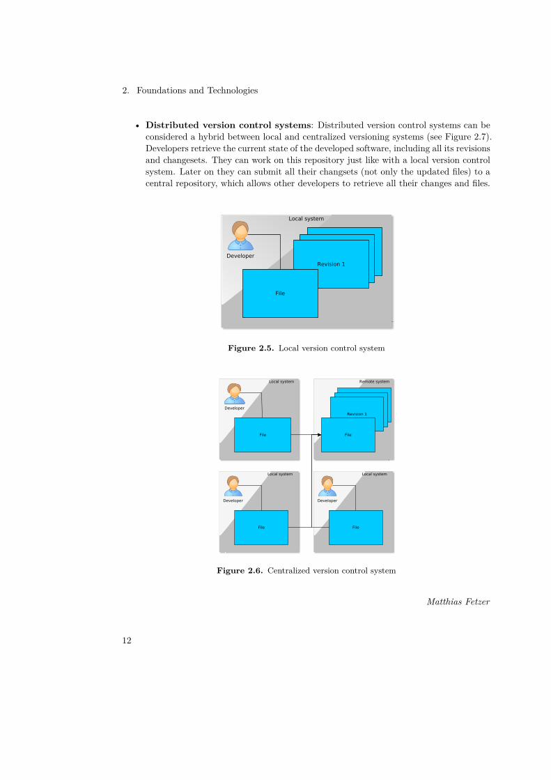
• Local version control systems: The easiest way of keeping several revisions of afile is, to manually create copies of the files the developer is working on (see Figure 2.5).All the changes and revisions are only available to the developer who created thoserevisions. This allows the developer to revert back to any state he (explicitly) saved.
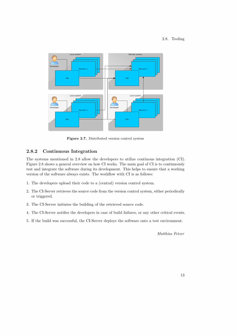
• Centralized version control systems: Centralized version control keeps revisions(or changesets) at a central location (see Figure 2.6). Developers retrieve the currentversion and later on submit their changes. This allows several developers to work onthe same files at the same time.
11
2. Foundations and Technologies
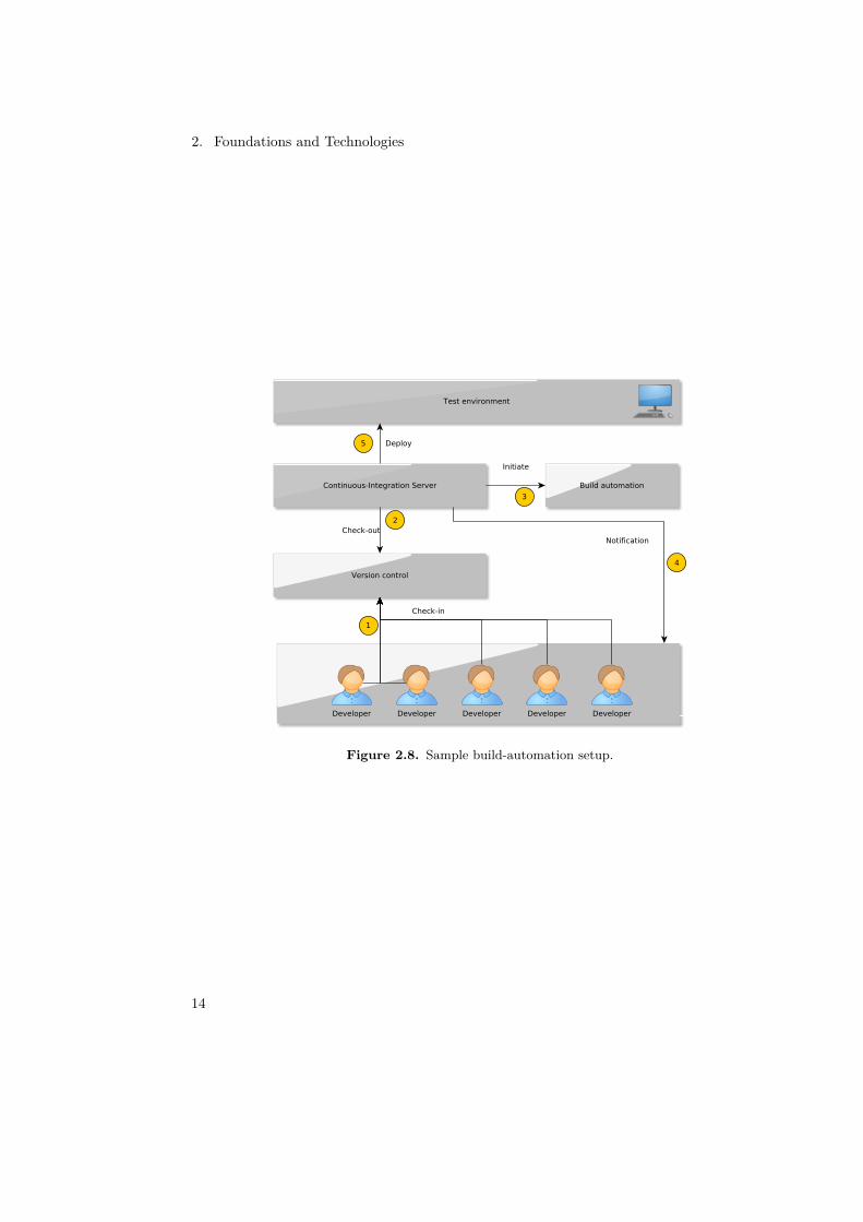
• Distributed version control systems: Distributed version control systems can beconsidered a hybrid between local and centralized versioning systems (see Figure 2.7).Developers retrieve the current state of the developed software, including all its revisionsand changesets. They can work on this repository just like with a local version controlsystem. Later on they can submit all their changsets (not only the updated files) to acentral repository, which allows other developers to retrieve all their changes and files.
Figure 2.5. Local version control system
Figure 2.6. Centralized version control system
Matthias Fetzer
12
2.8. Tooling
Figure 2.7. Distributed version control system
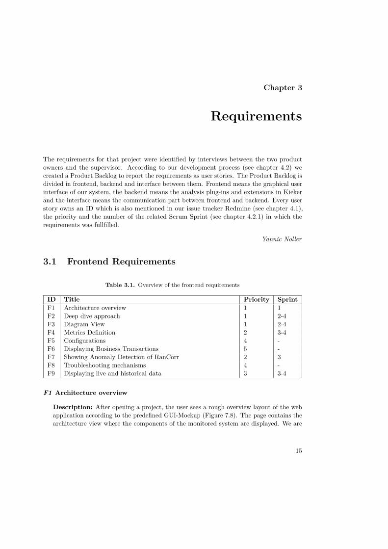
2.8.2 Continuous IntegrationThe systems mentioned in 2.8 allow the developers to utilize continous integration (CI).Figure 2.8 shows a general overview on how CI works. The main goal of CI is to continuouslytest and integrate the software during its development. This helps to ensure that a workingversion of the software always exists. The workflow with CI is as follows:
1. The developers upload their code to a (central) version control system.
2. The CI-Server retrieves the source code from the version control system, either periodicallyor triggered.
3. The CI-Server initiates the building of the retrieved source code.
4. The CI-Server notifies the developers in case of build failures, or any other critical events.
5. If the build was successful, the CI-Server deploys the software onto a test environment.
Matthias Fetzer
13
2. Foundations and Technologies
Figure 2.8. Sample build-automation setup.
14
Chapter 3
Requirements
The requirements for that project were identified by interviews between the two productowners and the supervisor. According to our development process (see chapter 4.2) wecreated a Product Backlog to report the requirements as user stories. The Product Backlog isdivided in frontend, backend and interface between them. Frontend means the graphical userinterface of our system, the backend means the analysis plug-ins and extensions in Kiekerand the interface means the communication part between frontend and backend. Every userstory owns an ID which is also mentioned in our issue tracker Redmine (see chapter 4.1),the priority and the number of the related Scrum Sprint (see chapter 4.2.1) in which therequirements was fullfilled.
Yannic Noller
3.1 Frontend Requirements
Table 3.1. Overview of the frontend requirements
ID Title Priority SprintF1 Architecture overview 1 1F2 Deep dive approach 1 2-4F3 Diagram View 1 2-4F4 Metrics Definition 2 3-4F5 Configurations 4 -F6 Displaying Business Transactions 5 -F7 Showing Anomaly Detection of RanCorr 2 3F8 Troubleshooting mechanisms 4 -F9 Displaying live and historical data 3 3-4
F1 Architecture overview
Description: After opening a project, the user sees a rough overview layout of the webapplication according to the predefined GUI-Mockup (Figure 7.8). The page contains thearchitecture view where the components of the monitored system are displayed. We are
15
3. Requirements
required to check whether the graph component of the existing Kieker WebGUI is suitiblefor our purpose. The diagram view and the tab view which should not be implemented,must be considered when designing the layout. A sub-requirement by the supervisor is touse the existing Kieker WebGUI which must be reduced to a basic level.
Acceptance Criteria: A first runnable prototype of the web application should be theoutcome of this requirement. The architecture view should display its first componentson the highest level(servers).
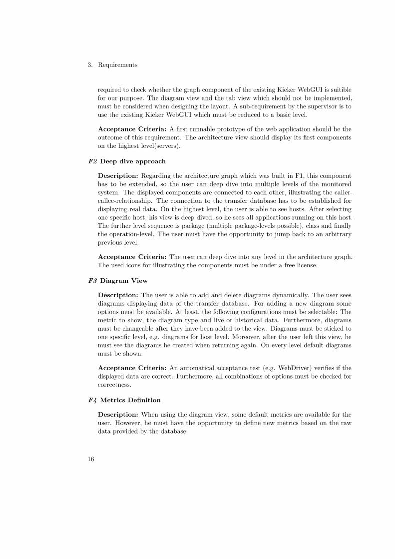
F2 Deep dive approach
Description: Regarding the architecture graph which was built in F1, this componenthas to be extended, so the user can deep dive into multiple levels of the monitoredsystem. The displayed components are connected to each other, illustrating the caller-callee-relationship. The connection to the transfer database has to be established fordisplaying real data. On the highest level, the user is able to see hosts. After selectingone specific host, his view is deep dived, so he sees all applications running on this host.The further level sequence is package (multiple package-levels possible), class and finallythe operation-level. The user must have the opportunity to jump back to an arbitraryprevious level.
Acceptance Criteria: The user can deep dive into any level in the architecture graph.The used icons for illustrating the components must be under a free license.
F3 Diagram View
Description: The user is able to add and delete diagrams dynamically. The user seesdiagrams displaying data of the transfer database. For adding a new diagram someoptions must be available. At least, the following configurations must be selectable: Themetric to show, the diagram type and live or historical data. Furthermore, diagramsmust be changeable after they have been added to the view. Diagrams must be sticked toone specific level, e.g. diagrams for host level. Moreover, after the user left this view, hemust see the diagrams he created when returning again. On every level default diagramsmust be shown.
Acceptance Criteria: An automatical acceptance test (e.g. WebDriver) verifies if thedisplayed data are correct. Furthermore, all combinations of options must be checked forcorrectness.
F4 Metrics Definition
Description: When using the diagram view, some default metrics are available for theuser. However, he must have the opportunity to define new metrics based on the rawdata provided by the database.
16
3.1. Frontend Requirements
Acceptance Criteria: If the user is able to define a new metric and he can choose thismetric to add a new diagram which is displayed correctly, this requirement is fulfilled.
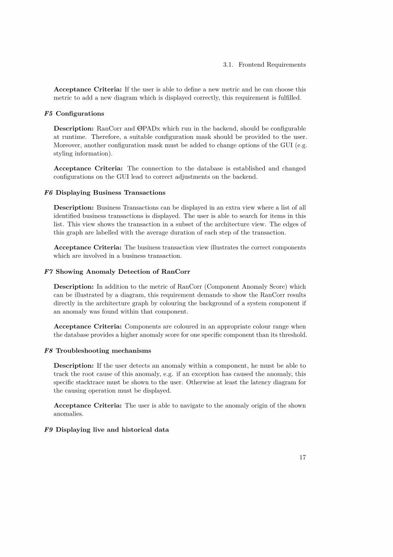
F5 Configurations
Description: RanCorr and ΘPADx which run in the backend, should be configurableat runtime. Therefore, a suitable configuration mask should be provided to the user.Moreover, another configuration mask must be added to change options of the GUI (e.g.styling information).
Acceptance Criteria: The connection to the database is established and changedconfigurations on the GUI lead to correct adjustments on the backend.
F6 Displaying Business Transactions
Description: Business Transactions can be displayed in an extra view where a list of allidentified business transactions is displayed. The user is able to search for items in thislist. This view shows the transaction in a subset of the architecture view. The edges ofthis graph are labelled with the average duration of each step of the transaction.
Acceptance Criteria: The business transaction view illustrates the correct componentswhich are involved in a business transaction.
F7 Showing Anomaly Detection of RanCorr
Description: In addition to the metric of RanCorr (Component Anomaly Score) whichcan be illustrated by a diagram, this requirement demands to show the RanCorr resultsdirectly in the architecture graph by colouring the background of a system component ifan anomaly was found within that component.
Acceptance Criteria: Components are coloured in an appropriate colour range whenthe database provides a higher anomaly score for one specific component than its threshold.
F8 Troubleshooting mechanisms
Description: If the user detects an anomaly within a component, he must be able totrack the root cause of this anomaly, e.g. if an exception has caused the anomaly, thisspecific stacktrace must be shown to the user. Otherwise at least the latency diagram forthe causing operation must be displayed.
Acceptance Criteria: The user is able to navigate to the anomaly origin of the shownanomalies.
F9 Displaying live and historical data
17
3. Requirements
Description: Regarding diagrams, the user has the possiblity to add a new diagramillustrating data monitored in a past time range or displaying live data. In the secondcase, the polling time of diagrams should be configurable. The architecture graph shouldalways work on live data. If a new component is instrumented by the backend and newlywritten into the database, the newly incoming component must also be displayed in thearchitecture graph.
Acceptance Criteria: The user is able to choose if live or historical data should bedisplayed in diagrams which then show the right time buckets. The architecture graph isdynamic including new components.
Anton Scherer
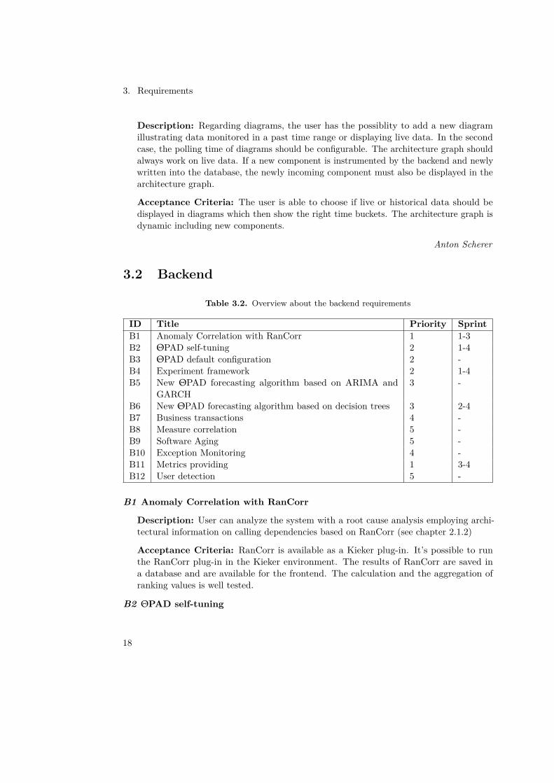
3.2 Backend
Table 3.2. Overview about the backend requirements
ID Title Priority SprintB1 Anomaly Correlation with RanCorr 1 1-3B2 ΘPAD self-tuning 2 1-4B3 ΘPAD default configuration 2 -B4 Experiment framework 2 1-4B5 New ΘPAD forecasting algorithm based on ARIMA and
GARCH3 -
B6 New ΘPAD forecasting algorithm based on decision trees 3 2-4B7 Business transactions 4 -B8 Measure correlation 5 -B9 Software Aging 5 -B10 Exception Monitoring 4 -B11 Metrics providing 1 3-4B12 User detection 5 -
B1 Anomaly Correlation with RanCorr
Description: User can analyze the system with a root cause analysis employing archi-tectural information on calling dependencies based on RanCorr (see chapter 2.1.2)
Acceptance Criteria: RanCorr is available as a Kieker plug-in. It’s possible to runthe RanCorr plug-in in the Kieker environment. The results of RanCorr are saved ina database and are available for the frontend. The calculation and the aggregation ofranking values is well tested.
B2 ΘPAD self-tuning
18
3.2. Backend
Description: ΘPAD shall be extended to be able to reconfigure itself.
Acceptance Criteria: It’s possible to run ΘPAD with an self-tuning algorithm, whichadjusts the configuration of ΘPAD at run-time. Therefore the filters of ΘPAD are nowconfigurable and there is an algorithm which automatically adjusts the configurations.The execution of this new combination of filters is well tested.
B3 ΘPAD default configuration
Description: ΘPAD shall be extended by a default configuration which can be used bythe user.
Acceptance Criteria: Default configuration for ΘPAD is identified, available andretrievable (especially for frontend).
B4 Experiment framework
Description: The analysis steps by ΘPAD and RanCorr shall be embedded in anexperiment framework to set the input of test data, change configurations, check testresults and provide appropriate test metrics.
Acceptance Criteria: There is an automatic input creation, execution, and outputevaluation for ΘPAD and RanCorr. The experiment framework runs and works.
B5 New ΘPAD forecasting algorithm based on ARIMA and GARCH
Description: ΘPAD shall be extended with a new forecast algorithm based on theintegration of ARIMA und GARCH models.
Acceptance Criteria: New forecast algorithm is available as extension of ΘPAD. Newforecast algorithm can be used in ΘPAD and is well tested.
B6 New ΘPAD forecasting algorithm based on decision trees
Description: ΘPAD shall be extended with a new forecast approach which selectssuitable forecast algorithms for a given context based on a decision tree and directfeedback cycles.
Acceptance Criteria: New forecast algorithm is available as extension of ΘPAD. Newforecast algorithm can be used in ΘPAD and is well tested.
B7 Business transactions
Description: Business transactions can be identified by the sequence of called methods(dynamic identification).
19

3. Requirements
Acceptance Criteria: Business Transaction Detection is available as Kieker plug-in.It’s runnable, works and is well tested. Business Transactions are stored in a databaseand is available for the frontend.
B8 Measure correlation
Description: The analysis shall be extended by a step which correlates multiple measures(e.g. response times and workload).
Acceptance Criteria: The analysis is available as a Kieker plug-in. It’s runnable, worksand is well tested. Results are stored in a database and are available for the frontend.
B9 Software Aging
Description: The analysis shall be extended to detect software aging.
Acceptance Criteria: New anomaly detection algorithm is available as a Kieker plug-in.It’s runnable, works and is well tested. Results are stored in a database and are availablefor the frontend.
B10 Exception Monitoring
Description: User can monitor various exceptions which occur in the monitored system.
Acceptance Criteria: Exceptions are monitored and stored in a database to providethem for the frontend. The Exception catching works and is well tested.
B11 Metrics providing
Description: User can access the monitored response times of operations, CPU load,memory usage (memory + swap), architecture, anomaly scores, anomaly rankings.
Acceptance Criteria: Response times of operations are monitored and stored in adatabase (accessible for the frontend). CPU load of all monitored machines are monitoredand stored in a database (accessible for the frontend). Memory usage (memory + swap)of all monitored machines are monitored and stored in a database (accessible for thefrontend). The architectures of all monitored machines are monitored and stored ina database (accessible for the frontend). Anomaly scores and anomaly rankings of allmonitored machines are monitored and stored in a database (accessible for the frontend).The backend uses the provided exchange interface (see I1) to transmit the data. Thedata exchange mechanism is documented and well tested.
B12 User detection
Description: It’s possible to detect which user is currently using the monitored systemand which operation calls are caused by that user.
20
3.3. Interface
Acceptance Criteria: Users are detected during run-time. It will be detected when anew user accesses the system and what he is actually doing, i.e. which operation callshe causes. It will also be detected when an user isn’t using the system anymore. A usershould be identified uniquely. The detection mechanism is documented and well tested.
Yannic Noller
3.3 Interface
Table 3.3. Overview about the interface requirements
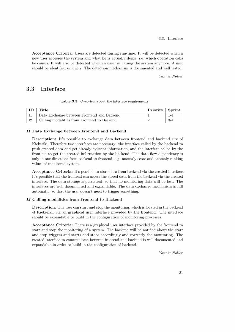
ID Title Priority SprintI1 Data Exchange between Frontend and Backend 1 1-4I2 Calling modalities from Frontend to Backend 2 3-4
I1 Data Exchange between Frontend and Backend
Description: It’s possible to exchange data between frontend and backend site ofKiekeriki. Therefore two interfaces are necessary: the interface called by the backend topush created data and get already existent information, and the interface called by thefrontend to get the created information by the backend. The data flow dependency isonly in one direction: from backend to frontend, e.g. anomaly score and anomaly rankingvalues of monitored system.
Acceptance Criteria: It’s possible to store data from backend via the created interface.It’s possible that the frontend can access the stored data from the backend via the createdinterface. The data storage is persistent, so that no monitoring data will be lost. Theinterfaces are well documented and expandable. The data exchange mechanism is fullautomatic, so that the user doesn’t need to trigger something.
I2 Calling modalities from Frontend to Backend
Description: The user can start and stop the monitoring, which is located in the backendof Kiekeriki, via an graphical user interface provided by the frontend. The interfaceshould be expandable to build in the configuration of monitoring processes.
Acceptance Criteria: There is a graphical user interface provided by the frontend tostart and stop the monitoring of a system. The backend will be notified about the startand stop triggers and starts and stops accordingly and correctly the monitoring. Thecreated interface to communicate between frontend and backend is well documented andexpandable in order to build in the configuration of backend.
Yannic Noller
21

Chapter 4
Project Management
4.1 ToolingThis section describes the underlying setup for the development project. The environmentfollows the continuous integration techniques and their requirements described in Section 2.8.
4.1.1 Hardware SpecificationThe tooling setup has been realized on a EX60-Server [Het, a] sponsored by Hetzner OnlineAG [Het, b].
The detailed hardware specifications are as follows:
• CPU: Intel(R) Core(TM) i7 CPU 920 (2.67GHz)• RAM: 48 GB DDR3 RAM• HDD: 2x 2TB (Western Digital WD2000FYYZ)
(in software raid1)• Bandwith: 1Gbit/s
Many thanks to Hetzner Online AG for the sponsorship.
Matthias Fetzer
4.1.2 Version Control SystemBefore the actual project started, the team had to chose between three, widely spread,version control systems:
• Git [Git] - A distributed version control system (see Section 2.8.1).• Mercurial [Mer] - A distributed version control system (see Section 2.8.1).• Apache Subversion [Sub] - A centralized version control system (see Section 2.8.1).
The team chose to use Git, as it offers, unlike SVN, a distributed version control. Furthermorethe team chose Git over Mercurial, as several team members had previous experience/exper-
23

4. Project Management
tise with Git.
The specific setup:
The specific setup was implemented on the dedicated server (see 4.1.1), using redmine (see4.1.3) to manage the repositories and the access control. Each sub-team obtained a dedicatedrepository:
• Backend• Documentation• Experiments• Frontend
Matthias Fetzer
4.1.3 Ticket-ManagementIn addition to the central administration of the source code, a stable and clear managementsystem is required for the organization of a large software project. For this purpose we couldchoose between two open source products "Trac" [Tra] and "Redmine" [Red]. They plotchanges to the source code while providing the possibility to link revisions with the projectplanning. The project plan is managed in this software and serves as a central informationplatform for developers.
Both Trac and Redmine are extensible through plugins and can be adapted to the in-dividual needs of the project stakeholders. Here, especially the longer established Trac ischaracterized by a large variety of enhancements that were developed for it in the course oftime. But many extensions, particularly useful for SCRUM, are not under active developmentand can only be used with older versions of Trac. As a result of the recently mentionedinformation and our positive experiences, the stakeholders chose to use Redmine.
Redmine already provides useful modules in its original state and requires little con-figuration effort before operational capability. To link Redmine to the continuous integrationsystem, provide advanced integration into development environments and enhance usability,the following plugins were installed.
• Redmine Git Hosting Plugin v0.6.2• Redmine Hudson plugin v2.1.2• Redmine LaTeX MathJax v0.1.0• Mylyn Connector plugin v2.8.2• Redmine plugin views revisions plugin v0.0.1
24

4.1. Tooling
The most important plugin for the project tracking is the "Redmine Git hosting plugin"(RGHP). The RGHP acts as an interface between Redmine and the Git version control system(VCS), imports changes from the VCS and assigns them to the corresponding Redmine tickets.A fixed rule (git-hook) ensures that only commits can be sent to the VCS, which include aticket number and thus are clearly assigned. Because of this limitation, the developers areurged to commit progressions individually and thereby support clarity.
Figure 4.1. Redmine task example
As shown in Figure 4.1, backlog items defined by the organization staff were later dividedinto smaller subtasks to be assigned to individual developers. The backlog item shown inthis case "Backlog #18: B6 Forecast Algorithm: Decision Tree" includes the task "replaceextended forcasting filter (opadx) and to devlop new filter with wcf". The code changesreferenced by the RGHP can be observed and tracked in the "Associated revisions".Based on this information, the developers can set the status of the task and thus provideinformation to the public. For example the persons responsible for the test project orientthemselves on this information and can automatically receive e-mail when the state reachesa certain level if desired. The ticket states, we use are as follows:
25

4. Project Management
• New• In Progress• Resolved• Feedback• Closed• Rejected• Estimated
Furthermore Redmine is used to exchange generic information and how-tos via the integratedwiki and provide configuration files about the file and document module.
Andreas Eberlein
4.1.4 Build-ServerFor the most other necessary tools and server services we had alternatives, which werepresented to the stakeholders for decision. But there was no free usable alternative for thebuild server, who offered themselves for Java development. While with "Apache Continuum"[Apa] there are also other continuous integration environments, none of the project participantshad positive experience with those in the context of reliability and usability. Therefore weuse "Jenkins" [Jen] with the following custom plugins to automate and test our softwareprojects.
• Ant Plugin• Checkstyle Plug-in• Copy Artifact Plugin• FindBugs Plugin• Git Client Plugin• Git Plugin• Jenkins Redmine plugin• Maven Integration plugin• PMD Plug-in• Static Code Analysis Plug-ins
In Jenkins all parts of the project that are located in different Git repositories are createdand configured with the associated build scripts. Jenkins gets the current file content of eachrepository and executes the build script (Section 4.1.5) that produces results periodicallyto the defined periods. These results are reported in case of failure or unacceptable codequality to the developer who caused them, as well as Redmine, so that the errors can bequickly identified and resolved. The build can also be started manually from the Redmine-or the Jenkins user interface at any time.
Andreas Eberlein
26

4.1. Tooling
4.1.5 Build Automation
Build automation enables developers to automate certain tasks in software development,such as:
• Code compilation• Package generation• Unit testing• Automated deployment• Javadoc generation• Code-Style checking• etc.
There are several tools which can aid in achieving these tasks. During the project start theteam had to chose between the following build systems:
• Apache Ant[ant]• Apache Buildr[bui]• Gradle[gra]• Apache Maven[mav]
The team chose Maven as their build-tool, as a few team members had previous experiencewith Maven and because of its comfortable dependency management. Another advantage ofusing Maven was the amount of know how that can be obtained by searching the internet,compared to Buildr or Gradle. Besides the standard Java- and JUnit-plugins for Maven, weadditionally used the following plugins:
• Maven FindBugs Plugin[Mav, b]• Maven CheckStyle Plugin[Mav, a]• Maven PMD Plugin[Mav, c]
Matthias Fetzer
4.1.6 Supplemental Tooling
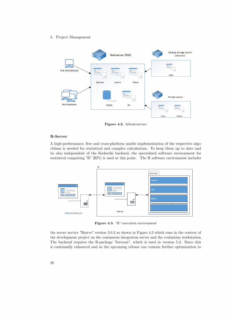
Besides the Java-tooling, other technical-infrastructure tasks had to be set up and maintained.This section gives an overview of the accomplished tasks, which were not covered in thesections above. Figure 4.2 shows an overview of the complete infrastructure that we use forthe development project.
Andreas Eberlein
27
4. Project Management
Figure 4.2. Infrastructure
R-Server
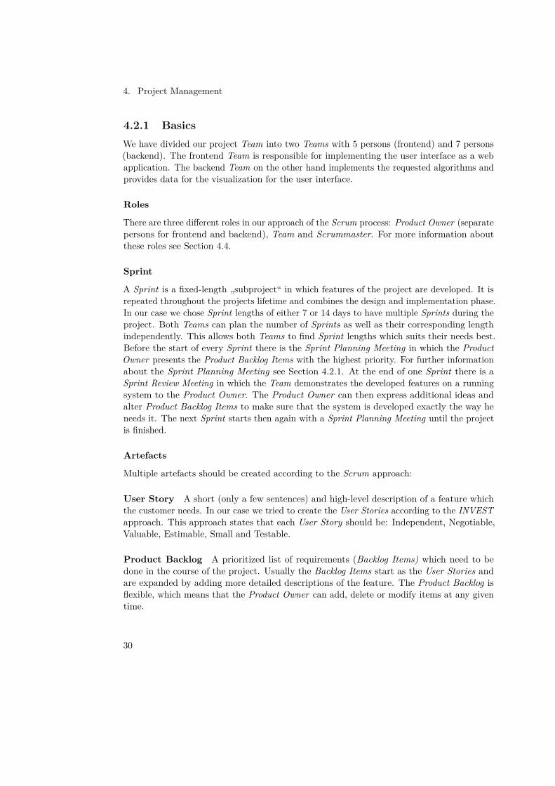
A high-performance, free and cross-platform usable implementation of the respective algo-rithms is needed for statistical and complex calculations. To keep them up to date andbe also independent of the Kiekeriki backend, the specialized software environment forstatistical computing "R" [RPr] is used at this point. The R software environment includes
Figure 4.3. "R" execution environment
the server service "Rserve" version 3.0.3 as shown in Figure 4.3 which runs in the context ofthe development project on the continuous integration server and the evaluation workstation.The backend requires the R-package "forecast", which is used in version 5.3. Since thisis continually enhanced and as the upcoming release can contain further optimization to
28

4.2. Scrum
forecasters, especially this should be kept up to date.
The service "Rserve" has to be run on the same server on which the Kiekeriki backend isrunning due to the fixed local destination address in ΘPAD.
Andreas Eberlein
SQL-Server
Due to the fact that the communication between the frondend and backend is realizedvia a central SQL-Database, a MySQL-Server has been installed (and slightly tuned forperformance with the help of mysqltuner[mys].
Matthias Fetzer
Disaster Recovery
To ensure that the team can continue to work in case of a hardware or software failure, thefollowing (automated) backup mechanisms have been installed:
• Semi-hourly backups of the MySQL-Databases and its procedures via mysqldump.• Daily file-based backups to the backup-storage located at the Hetzner-Datacenter.• Daily file-based backups to a Backup-System, located at a private appartement.
The file-based backups have been done with rsnapshot1. This enables us to keep severalrevisions of all changed files, even the ones which are not under git-version control. Theretention settings for rsnapshot are:
• 7 daily backups• 4 weekly backups• 12 monthly backups
Matthias Fetzer
4.2 ScrumIn order to produce good results in the short time of this project we decided to use an agilesoftware developing process. We chose scrum because it is a lightweight process structurewith few specifications and therefore customizable to our needs. The following subsectionsdescribe how scrum is implemented in our development project.
1http://www.rsnapshot.org/
29
4. Project Management
4.2.1 BasicsWe have divided our project Team into two Teams with 5 persons (frontend) and 7 persons(backend). The frontend Team is responsible for implementing the user interface as a webapplication. The backend Team on the other hand implements the requested algorithms andprovides data for the visualization for the user interface.
Roles
There are three different roles in our approach of the Scrum process: Product Owner (separatepersons for frontend and backend), Team and Scrummaster. For more information aboutthese roles see Section 4.4.
Sprint
A Sprint is a fixed-length „subproject“ in which features of the project are developed. It isrepeated throughout the projects lifetime and combines the design and implementation phase.In our case we chose Sprint lengths of either 7 or 14 days to have multiple Sprints during theproject. Both Teams can plan the number of Sprints as well as their corresponding lengthindependently. This allows both Teams to find Sprint lengths which suits their needs best.Before the start of every Sprint there is the Sprint Planning Meeting in which the ProductOwner presents the Product Backlog Items with the highest priority. For further informationabout the Sprint Planning Meeting see Section 4.2.1. At the end of one Sprint there is aSprint Review Meeting in which the Team demonstrates the developed features on a runningsystem to the Product Owner. The Product Owner can then express additional ideas andalter Product Backlog Items to make sure that the system is developed exactly the way heneeds it. The next Sprint starts then again with a Sprint Planning Meeting until the projectis finished.
Artefacts
Multiple artefacts should be created according to the Scrum approach:
User Story A short (only a few sentences) and high-level description of a feature whichthe customer needs. In our case we tried to create the User Stories according to the INVESTapproach. This approach states that each User Story should be: Independent, Negotiable,Valuable, Estimable, Small and Testable.
Product Backlog A prioritized list of requirements (Backlog Items) which need to bedone in the course of the project. Usually the Backlog Items start as the User Stories andare expanded by adding more detailed descriptions of the feature. The Product Backlog isflexible, which means that the Product Owner can add, delete or modify items at any giventime.
30
4.2. Scrum
Sprint Backlog The Sprint Backlog contains the items which will be developed during thecurrent Sprint. After the Sprint Planning Meeting a list of Backlog Items are removed fromthe Product Backlog and added to the Sprint Backlog. Compared to the Product Backlog theSprint Backlog is a lot smaller and, more importantly, not flexible. This means that items inthe Sprint Backlog can not be altered, removed or added. This leads to stable requirementsfor the developers which in turn leads to better results because the developers do not needto change features while they are being implemented.
Meetings
Sprint Planning Meeting The Sprint Planning Meeting is always at the beginning of aSprint. During this meeting the Product Owner presents the high priority items from theProduct Backlog that need to be implemented next. He also gives more detailed informationand answers questions from the Team about the items. For every relevant Backlog Item theTeam then uses an approach called Planning Poker to estimate how many days are necessaryto implement this specific item. During the Planning Poker the developers simultaneouslyshow cards with a number on according to their estimated time requirement for a BacklogItem. The developers with highest and lowest estimation than discuss briefly (¤ 2 min) whythey chose their corresponding card. After that the whole Team estimates again. This isrepeated until every developer estimates the same amount (shows the same card). After allrelevant Backlog Items have been estimated the Team chooses a set of items which will beimplemented in the next Sprint and thereby move the items from the Product Backlog to theSprint Backlog. That, in turn, means that these items can not be modified any longer untilthe Sprint is finished.
Sprint Review Meeting This meeting is always at the end of a Sprint. Usually theTeam demonstrates the created features in a live demo to the Product Owners. Because bothProduct Owners are part of the Team this is not necessary in our project. Instead we discusshow much of our goals have been reached and whether or not it is necessary to re-insert andre-estimate specific items into the Sprint Backlog for the next Sprint.
Daily Scrum The Daily Scrum is a short (¤ 15min) Meeting that takes place every dayfor both groups separately. Each developer states what he has done since the last meeting,what he is about to do and (if necessary) what prevents him from doing so.
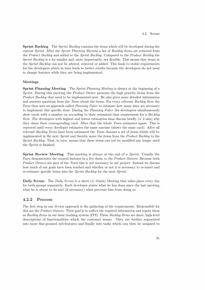
4.2.2 ProcessThe first step in our Scrum approach is the gathering of the requirements. Responsible forthis are the Product Owners. Their goal is to collect the required information and report themas Backlog Items in our issue tracking system (ITS). These Backlog Items are short, high-leveldescriptions of functionalities which the customer wants. They are further segmentedinto more fine-grained sub-features and finally into tasks which can then be assigned to
31
4. Project Management
Figure 4.4. Overview of the Scrum process
Team members. The segmentation and creation of tasks is done by the correspondingProduct Owners. This is not necessarily applicable for every Scrum-related project, butin our case we have the advantage that the Product Owners are developers as well andcan therefore reckon which sub-features and tasks are necessary to implement the functionality.
After the initial set of sub-features and tasks are created the first Sprint starts. At thebeginning of the Sprint there is always a Sprint Planning Meeting where the Teams estimateand choose the features which will be implemented. During the Sprint both Teams work onthe items in the Sprint Backlog and have separate Daily Scrums every day to keep everyTeam member informed about the current progress. See also Figure 4.4
At the end of the Sprint there is the Sprint Review Meeting as discussed previously(Section 4.2.1). Furthermore, every Sprint Backlog Item should be completed by that time.Otherwise it needs to be transferred into the Sprint Backlog for the upcoming Sprint.
4.2.3 Sprint Overview
The following shows the Sprints as well as the tasks which were chosen by both Teams.
32
4.2. Scrum
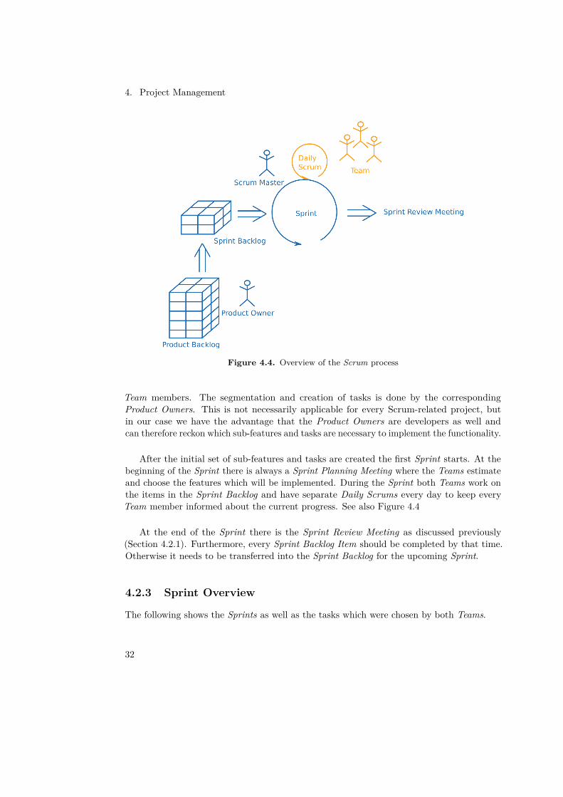
Figure 4.5. Sprints for both Teams during the project.
Table 4.1. This table shows the backend tasks and when they were completed.
Backlog Item Task SprintRanCorr Implement RanCorr BS1
Provide Kieker Plug-In BS1Database extension BS3
Self-Tuning Implement runtime configuration BS1Develop composite filter plugin BS3
Default-Configuration Find and provide default values BS5Experiment Framework Identify format of testdata BS1
Manually build testdata BS2Automatically build testdata BS3Build experiment framework aroundΘ𝑃𝐴𝐷 and RanCorr
BS4
Automate evaluation of Θ𝑃𝐴𝐷 and Ran-Corr
BS4
Forecast Algorithm: Decision Tree Implement WCF BS4Replace existing forecaster BS4
Various Metric Monitoring Store CPU Load BS4Store RAM Load BS4Store Swap Load BS4Store Latencies BS4
33

4. Project Management
Table 4.2. This table shows the frontend tasks and when they were completed.
Backlog Item Task SprintArchitecture Overview Create clean Web-GUI version FS1
Create dashboard overview FS1Display aggregated information FS1Get data from DB FS1GUI sketch FS1
Deep dive approach Build model FS2Connection to transfer DB FS4Extend architecture view FS4
Diagram View Create diagrams dynamically FS2Database connection for diagrams FS2Create configuration dialogue FS3Save diagram config in DB FS3
Metrics Definition Define default metrics FS3Create settings tab content FS4
Showing Anomaly Detection (RanCorr) Show results in architecture graph FS3Displaying live and historical data Display current data in architecture
graphFS3
Implement polling mechanism for di-agrams
FS4
Dominik Olp
4.3 Team
In the following is a mapping of the most important tasks during the project’s lifetime andthe corresponding team members who worked on it.
Table 4.3. Legend
l worked mainly on this itemm worked partially on this item
didn’t work on this item
34
4.3. Team
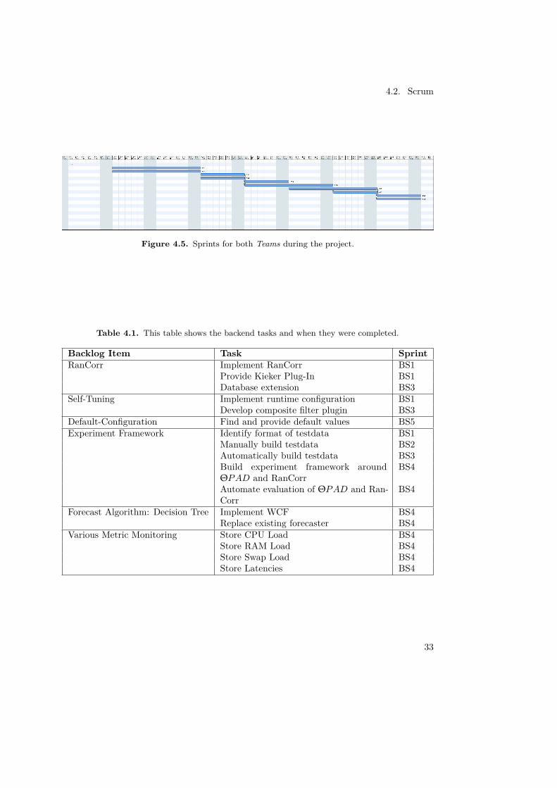
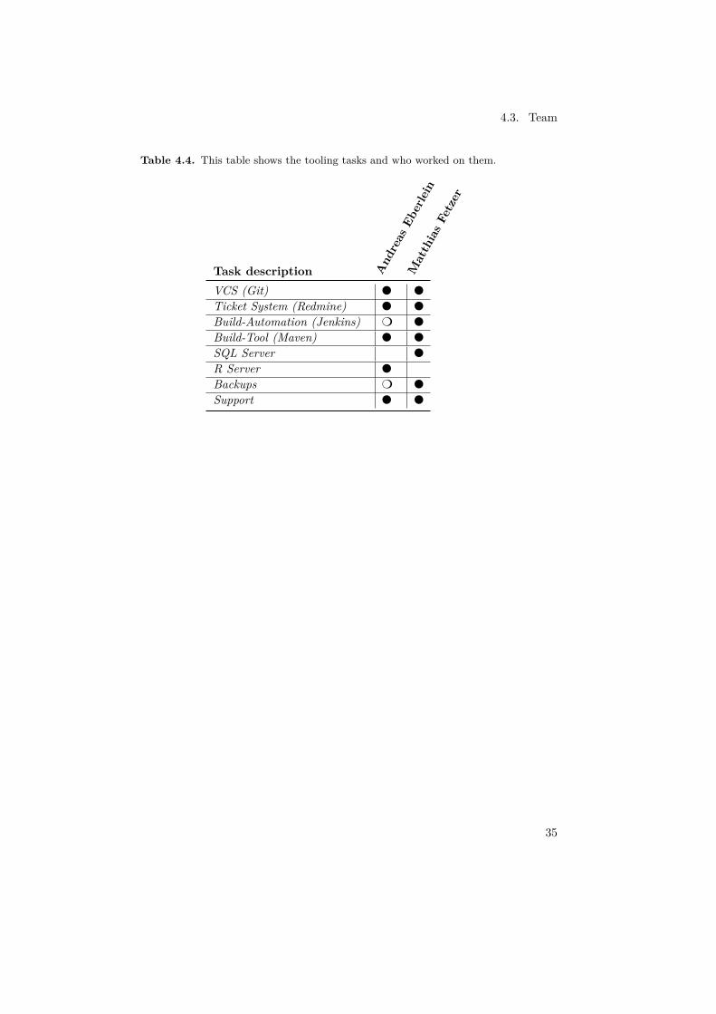
Table 4.4. This table shows the tooling tasks and who worked on them.
Task description And
reas
Eber
lein
Mat
thia
sFe
tzer
VCS (Git) l l
Ticket System (Redmine) l l
Build-Automation (Jenkins) m l
Build-Tool (Maven) l l
SQL Server l
R Server l
Backups m l
Support l l
35
4. Project Management
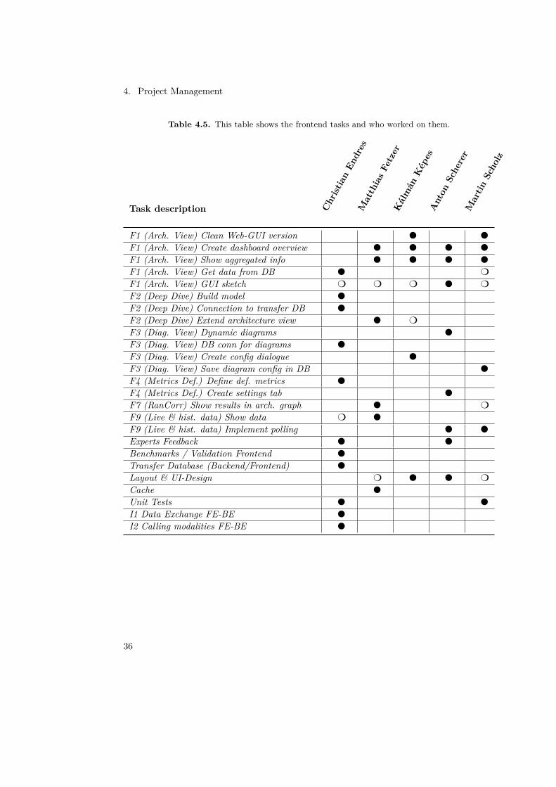
Table 4.5. This table shows the frontend tasks and who worked on them.
Task description Chr
istia
nEn
dres
Mat
thia
sFe
tzer
Kál
mán
Kép
esA
nton
Sche
rer
Mar
tinSc
holz
F1 (Arch. View) Clean Web-GUI version l l
F1 (Arch. View) Create dashboard overview l l l l
F1 (Arch. View) Show aggregated info l l l l
F1 (Arch. View) Get data from DB l m
F1 (Arch. View) GUI sketch m m m l m
F2 (Deep Dive) Build model l
F2 (Deep Dive) Connection to transfer DB l
F2 (Deep Dive) Extend architecture view l m
F3 (Diag. View) Dynamic diagrams l
F3 (Diag. View) DB conn for diagrams l
F3 (Diag. View) Create config dialogue l
F3 (Diag. View) Save diagram config in DB l
F4 (Metrics Def.) Define def. metrics l
F4 (Metrics Def.) Create settings tab l
F7 (RanCorr) Show results in arch. graph l m
F9 (Live & hist. data) Show data m l
F9 (Live & hist. data) Implement polling l l
Experts Feedback l l
Benchmarks / Validation Frontend l
Transfer Database (Backend/Frontend) l
Layout & UI-Design m l l m
Cache l
Unit Tests l l
I1 Data Exchange FE-BE l
I2 Calling modalities FE-BE l
36
4.4. Roles
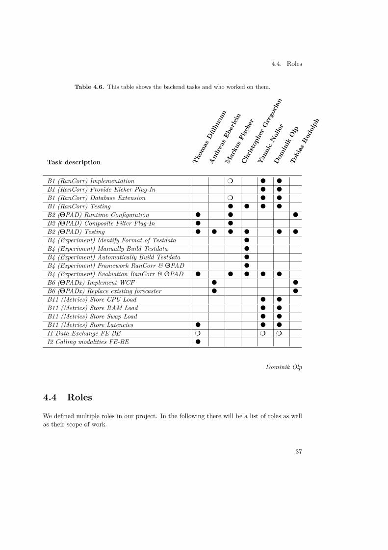
Table 4.6. This table shows the backend tasks and who worked on them.
Task description Thom
asD
üllm
ann
And
reas
Eber
lein
Mar
kus
Fisc
her
Chr
istop
her
Gre
goria
n
Yann
icN
olle
rD
omin
ikO
lpTo
bias
Rud
olph
B1 (RanCorr) Implementation m l l
B1 (RanCorr) Provide Kieker Plug-In l l
B1 (RanCorr) Database Extension m l l
B1 (RanCorr) Testing l l l l
B2 (ΘPAD) Runtime Configuration l l l
B2 (ΘPAD) Composite Filter Plug-In l l
B2 (ΘPAD) Testing l l l l l l
B4 (Experiment) Identify Format of Testdata l
B4 (Experiment) Manually Build Testdata l
B4 (Experiment) Automatically Build Testdata l
B4 (Experiment) Framework RanCorr & ΘPAD l
B4 (Experiment) Evaluation RanCorr & ΘPAD l l l l l
B6 (ΘPADx) Implement WCF l l
B6 (ΘPADx) Replace existing forecaster l l
B11 (Metrics) Store CPU Load l l
B11 (Metrics) Store RAM Load l l
B11 (Metrics) Store Swap Load l l
B11 (Metrics) Store Latencies l l l
I1 Data Exchange FE-BE m m m
I2 Calling modalities FE-BE l
Dominik Olp
4.4 Roles
We defined multiple roles in our project. In the following there will be a list of roles as wellas their scope of work.
37

4. Project Management
Quality Assurance Engineer: Enforces quality assurance measures. Makes sure alldevelopers write test cases for their corresponding area. Verifies that all developers writetheir code according to a common style guide.Responsible: Markus Fischer
Document Representative: Creates and maintains document structures. Additionally,takes care that all created documents are up to date. Makes sure documents get finished intime.Responsible: Martin Scholz
Product Owner(s): Act as the interface between the project Team and the supervisor/cus-tomer. They are responsible for creating and maintaining a list of requirements. Furthermore,they need to answer upcoming questions from the Team about requirements. Additionallythey decide the priority of requirements and therefore influence which requirements are dealtwith in any Sprint (for more information about Sprints and our development process see:Section 4.2).Responsible: Anton Scherer (Frontend), Yannic Noller (Backend)
Infrastructure Representative(s): Handle the infrastructure as well as the softwareneeded to realize the project. Especially following topics are under the supervision of theinfrastructure representatives:
• Set-up and maintenance of a versioning system• Integrating issue tracker• Set-up of a buildsystem• Enable continuous integration & automated testing• Set-up and maintenance of databases
Responsible: Andreas Eberlein, Matthias Fetzer
Scrummaster/Projectleader: Enforces a scrum-conform approach and acts as a mod-erator in meetings to avoid long discussion and thereby ensures that time constraints aremet.Responsible: Dominik Olp
Developer (aka Team): Implementation of the requirements specified by the ProductOwner.Responsible: Everybody
Dominik Olp
38
Chapter 5
Architecture and Concepts
Due to the different foundations front- and backend are based on, the architecture chapter issplit in separate sections. To put them into context, we will give an overview first.
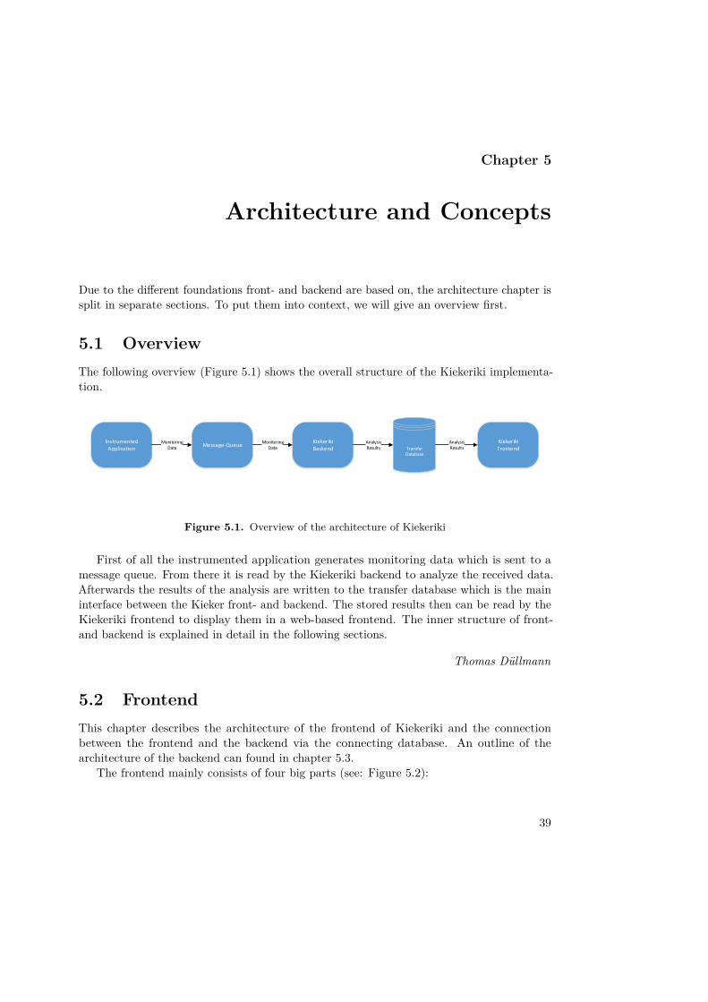
5.1 OverviewThe following overview (Figure 5.1) shows the overall structure of the Kiekeriki implementa-tion.
Message-QueueTransferDatabase
InstrumentedApplication
KiekerikiBackend
KiekerikiFrontend
MonitoringData
MonitoringData
AnalysisResults
AnalysisResults
Figure 5.1. Overview of the architecture of Kiekeriki
First of all the instrumented application generates monitoring data which is sent to amessage queue. From there it is read by the Kiekeriki backend to analyze the received data.Afterwards the results of the analysis are written to the transfer database which is the maininterface between the Kieker front- and backend. The stored results then can be read by theKiekeriki frontend to display them in a web-based frontend. The inner structure of front-and backend is explained in detail in the following sections.
Thomas Düllmann
5.2 FrontendThis chapter describes the architecture of the frontend of Kiekeriki and the connectionbetween the frontend and the backend via the connecting database. An outline of thearchitecture of the backend can found in chapter 5.3.
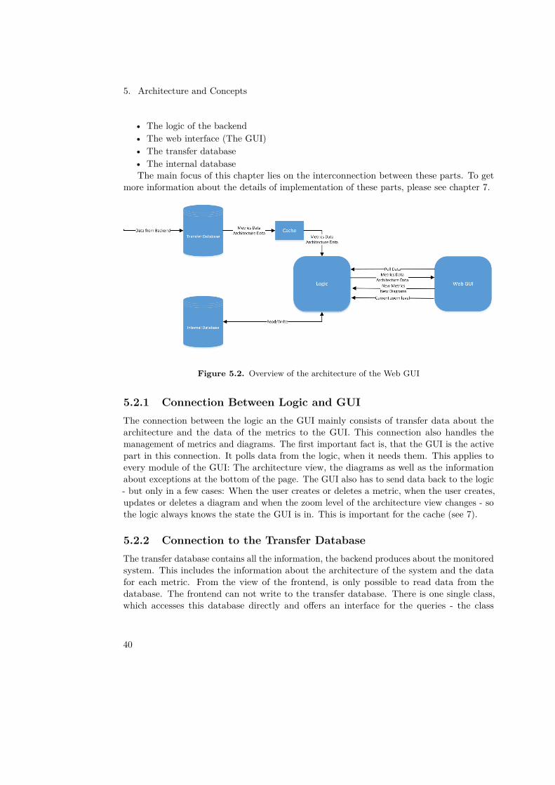
The frontend mainly consists of four big parts (see: Figure 5.2):
39
5. Architecture and Concepts
• The logic of the backend• The web interface (The GUI)• The transfer database• The internal databaseThe main focus of this chapter lies on the interconnection between these parts. To get
more information about the details of implementation of these parts, please see chapter 7.
Figure 5.2. Overview of the architecture of the Web GUI
5.2.1 Connection Between Logic and GUIThe connection between the logic an the GUI mainly consists of transfer data about thearchitecture and the data of the metrics to the GUI. This connection also handles themanagement of metrics and diagrams. The first important fact is, that the GUI is the activepart in this connection. It polls data from the logic, when it needs them. This applies toevery module of the GUI: The architecture view, the diagrams as well as the informationabout exceptions at the bottom of the page. The GUI also has to send data back to the logic- but only in a few cases: When the user creates or deletes a metric, when the user creates,updates or deletes a diagram and when the zoom level of the architecture view changes - sothe logic always knows the state the GUI is in. This is important for the cache (see 7).
5.2.2 Connection to the Transfer DatabaseThe transfer database contains all the information, the backend produces about the monitoredsystem. This includes the information about the architecture of the system and the datafor each metric. From the view of the frontend, is only possible to read data from thedatabase. The frontend can not write to the transfer database. There is one single class,which accesses this database directly and offers an interface for the queries - the class
40
5.3. Backend
DatabasePlainConnection. To reduce the load of the database, there is a cache between allthe components, which needs data of the database and the DatabasePlainConnection. Thiscache holds all information, which were already queried in its memory for a certain amountof time. Components, which query data, get the data from the memory of the cache insteadof directly from the database. Only if the data is outdated (which is defined differently fordifferent types of data), the cache fetches the new data from database before returning themto the component, which queries for it.
5.2.3 Connection to the Internal DatabaseFor the storage of diagrams and the metrics, the internal database is used, which was alreadyused by Kieker to store user related data. Two new tables, one for the metrics and one forthe diagrams were added to fit our needs. Each diagram is related to one metric and eachmetric is related to one user.
Martin Scholz
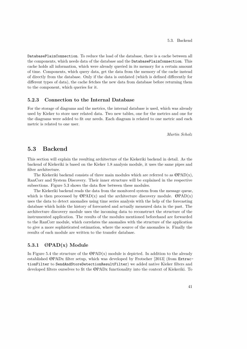
5.3 BackendThis section will explain the resulting architecture of the Kiekeriki backend in detail. As thebackend of Kiekeriki is based on the Kieker 1.8 analysis module, it uses the same pipes andfilter architecture.
The Kiekeriki backend consists of three main modules which are referred to as ΘPAD(x),RanCorr and System Discovery. Their inner structure will be explained in the respectivesubsections. Figure 5.3 shows the data flow between these modules.
The Kiekeriki backend reads the data from the monitored system from the message queue,which is then processed by ΘPAD(x) and the architecture discovery module. ΘPAD(x)uses the data to detect anomalies using time series analysis with the help of the forecastingdatabase which holds the history of forecasted and actually measured data in the past. Thearchitecture discovery module uses the incoming data to reconstruct the structure of theinstrumented application. The results of the modules mentioned beforehand are forwardedto the RanCorr module, which correlates the anomalies with the structure of the applicationto give a more sophisticated estimation, where the source of the anomalies is. Finally theresults of each module are written to the transfer database.
5.3.1 ΘPAD(x) ModuleIn Figure 5.4 the structure of the ΘPAD(x) module is depicted. In addition to the alreadyestablished ΘPADx filter setup, which was developed by Frotscher [2013] (from Extrac-tionFilter to SendAndStoreDetectionResultFilter) we added native Kieker filters anddeveloped filters ourselves to fit the ΘPADx functionality into the context of Kiekeriki. To
41
5. Architecture and Concepts
Message-QueueTransferDatabase
InstrumentedApplication
KiekerikiBackend
KiekerikiFrontend
MonitoringData
MonitoringData
AnalysisResults
AnalysisResults
Kiekeriki Backend
ΘPAD(x)
RanCorr
ArchitectureDiscovery
Forecasting Database
Figure 5.3. Overview of the architecture of Kiekeriki backend
easily use the ΘPADx functionality, we developed a composite filter plugin that wraps theoriginal ΘPADx functionality in one single filter.
The following diagram (Figure 5.4) and list explains shortly what the filters that havebeen added to the original ΘPADx approach do. As the ΘPADx has been explained in detailby Frotscher [2013]. The corresponding filters are ommited in the listing.
• JMSReaderReads the monitored data from a Java Message Service (JMS) message queue.
• RecordConverterConverts the incoming OperationExecution information to an ΘPADx-compatibleformat.
• StringBufferFilterBuffers strings to optimize memory usage.
• ΘPADx Filters
• OpadOutputCompositionFilterCreates output objects that contain all information that ΘPADx can provide from theincoming data.
42
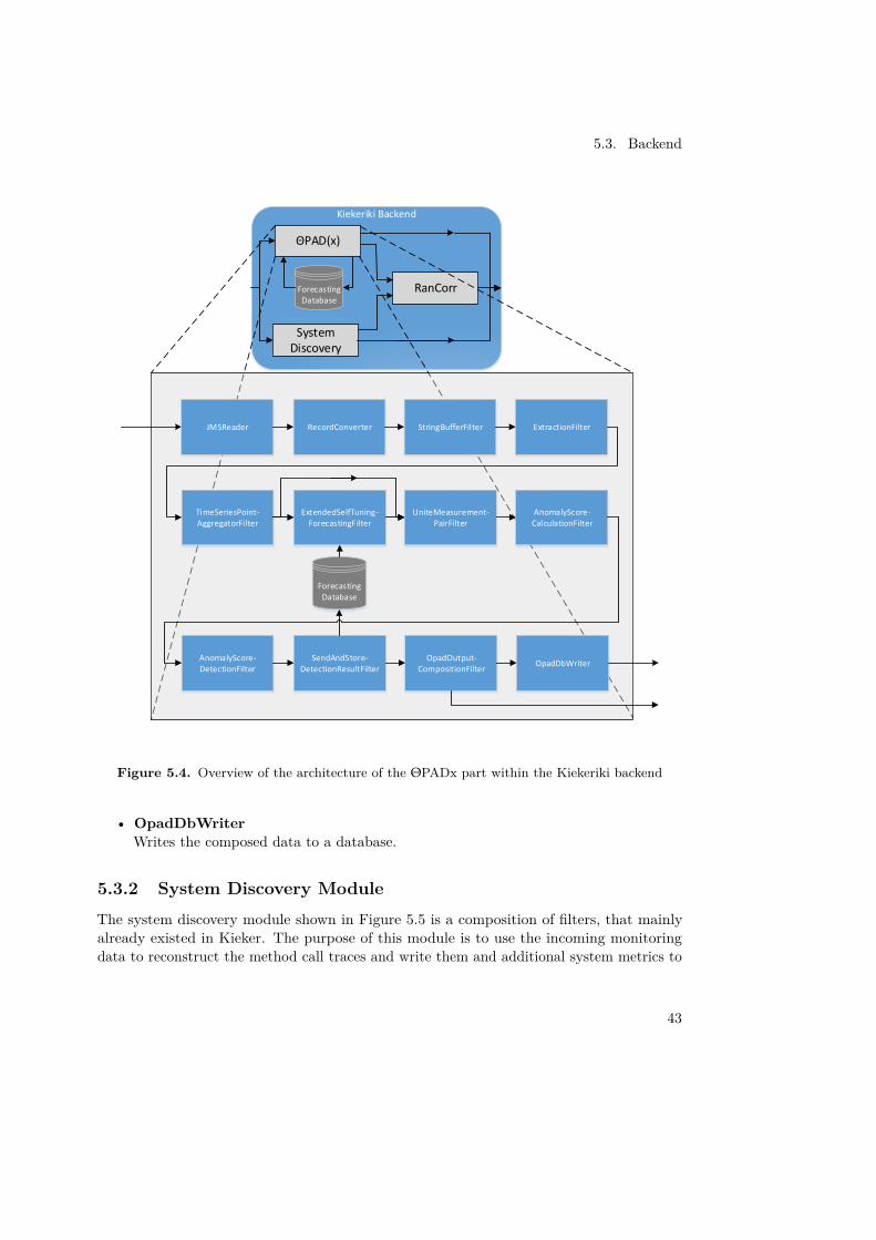
5.3. Backend
Kiekeriki Backend
ΘPAD(x)
RanCorr
SystemDiscovery
Forecasting Database
Forecasting Database
JMSReader RecordConverter StringBufferFilter ExtractionFilter
TimeSeriesPoint-AggregatorFilter
ExtendedSelfTuning-ForecastingFilter
UniteMeasurement-PairFilter
AnomalyScore-CalculationFilter
AnomalyScore-DetectionFilter
SendAndStore-DetectionResultFilter
OpadOutput-CompositionFilter
OpadDbWriter
Figure 5.4. Overview of the architecture of the ΘPADx part within the Kiekeriki backend
• OpadDbWriterWrites the composed data to a database.
5.3.2 System Discovery ModuleThe system discovery module shown in Figure 5.5 is a composition of filters, that mainlyalready existed in Kieker. The purpose of this module is to use the incoming monitoringdata to reconstruct the method call traces and write them and additional system metrics to
43
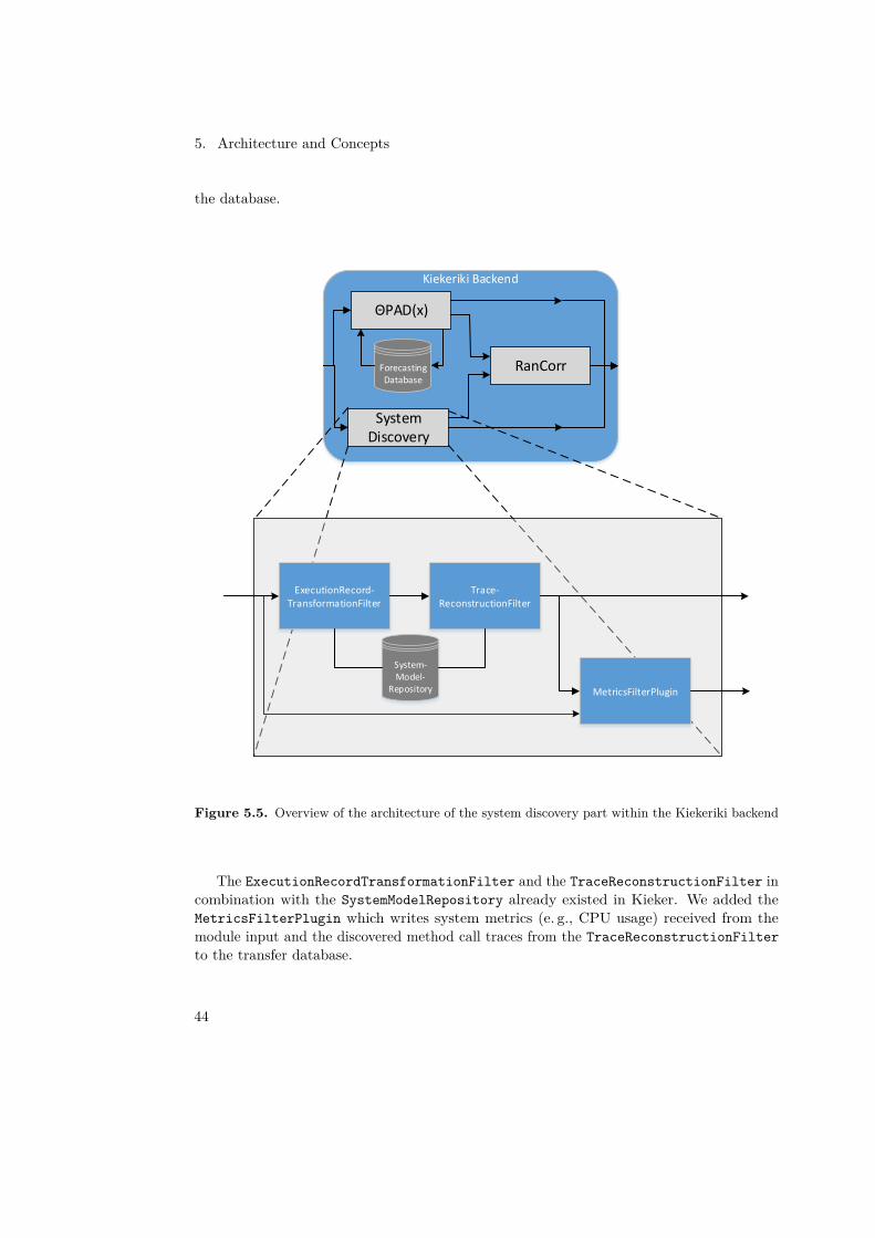
5. Architecture and Concepts
the database.
Kiekeriki Backend
ΘPAD(x)
RanCorr
SystemDiscovery
Forecasting Database
ExecutionRecord-TransformationFilter
Trace-ReconstructionFilter
System-Model-
Repository MetricsFilterPlugin
Figure 5.5. Overview of the architecture of the system discovery part within the Kiekeriki backend
The ExecutionRecordTransformationFilter and the TraceReconstructionFilter incombination with the SystemModelRepository already existed in Kieker. We added theMetricsFilterPlugin which writes system metrics (e. g., CPU usage) received from themodule input and the discovered method call traces from the TraceReconstructionFilterto the transfer database.
44

5.3. Backend
5.3.3 RanCorr ModuleThe RanCorr module shown in Figure 5.6 uses the anomaly scores from the ΘPAD(x) moduleand the operation calls from the system discovery module to calculate RanCorr ranks.
Kiekeriki Backend
ΘPAD(x)
RanCorr
SystemDiscovery
Forecasting Database
RanCorrFilterRanCorrOutput-
DBWriter
Figure 5.6. Overview of the architecture of the RanCorr part within the Kiekeriki backend
The RanCorrFilter implements the RanCorr approach developed by Marwede et al.[2009] and the RanCorrOutputDBWriter writes the results of the RanCorrFilter to thetransfer database.
Thomas Düllmann
45
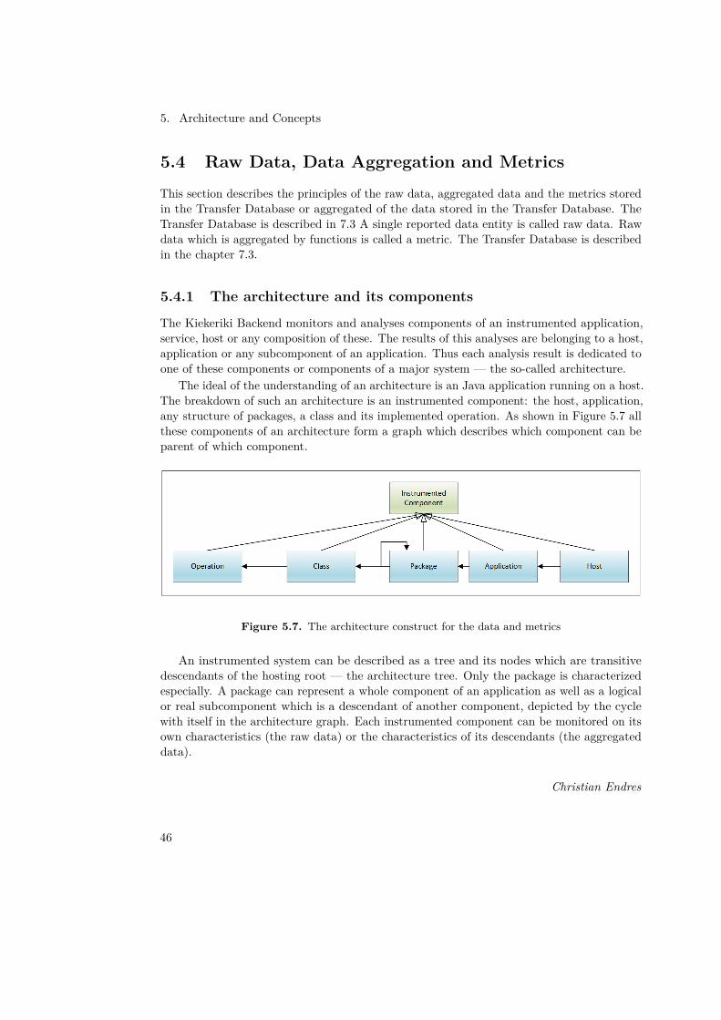
5. Architecture and Concepts
5.4 Raw Data, Data Aggregation and Metrics
This section describes the principles of the raw data, aggregated data and the metrics storedin the Transfer Database or aggregated of the data stored in the Transfer Database. TheTransfer Database is described in 7.3 A single reported data entity is called raw data. Rawdata which is aggregated by functions is called a metric. The Transfer Database is describedin the chapter 7.3.
5.4.1 The architecture and its components
The Kiekeriki Backend monitors and analyses components of an instrumented application,service, host or any composition of these. The results of this analyses are belonging to a host,application or any subcomponent of an application. Thus each analysis result is dedicated toone of these components or components of a major system — the so-called architecture.
The ideal of the understanding of an architecture is an Java application running on a host.The breakdown of such an architecture is an instrumented component: the host, application,any structure of packages, a class and its implemented operation. As shown in Figure 5.7 allthese components of an architecture form a graph which describes which component can beparent of which component.
Figure 5.7. The architecture construct for the data and metrics
An instrumented system can be described as a tree and its nodes which are transitivedescendants of the hosting root — the architecture tree. Only the package is characterizedespecially. A package can represent a whole component of an application as well as a logicalor real subcomponent which is a descendant of another component, depicted by the cyclewith itself in the architecture graph. Each instrumented component can be monitored on itsown characteristics (the raw data) or the characteristics of its descendants (the aggregateddata).
Christian Endres
46
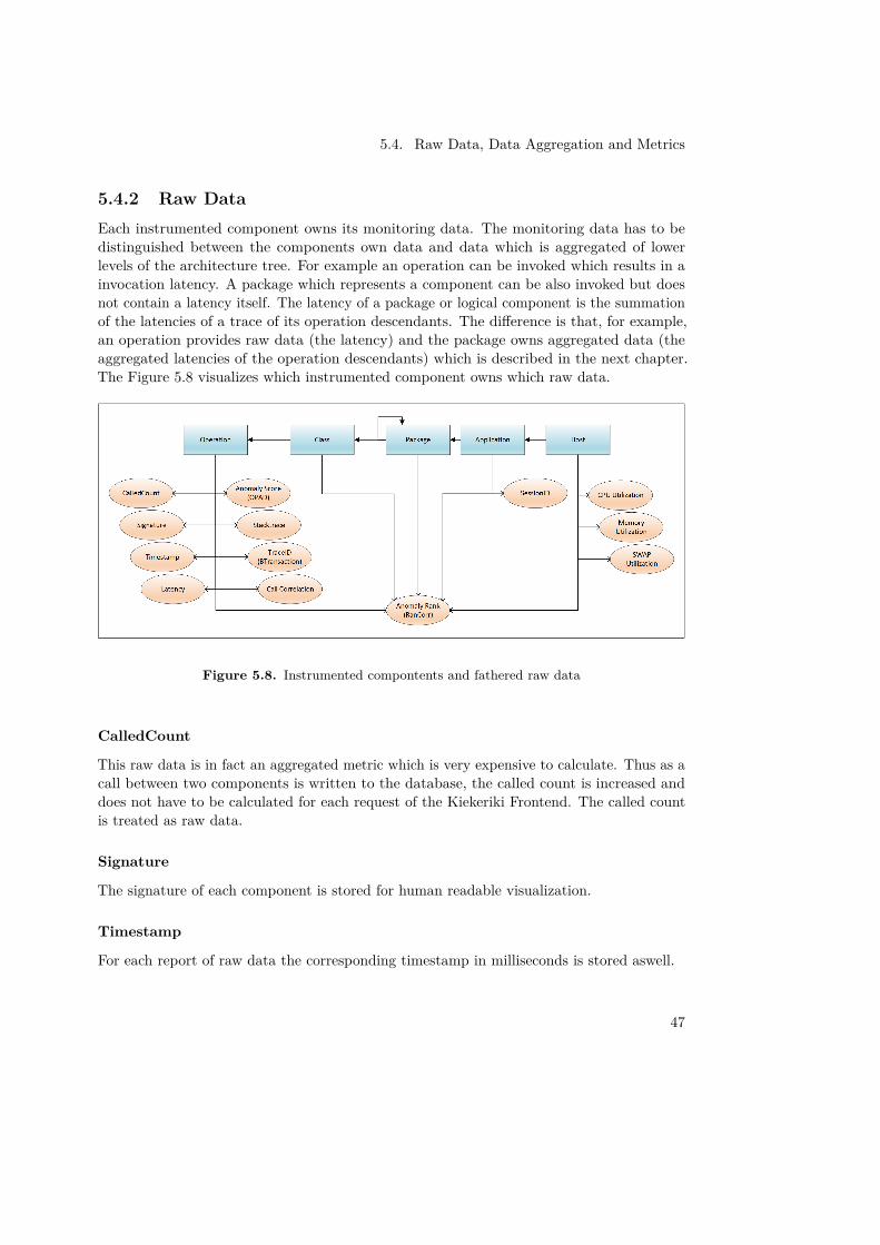
5.4. Raw Data, Data Aggregation and Metrics
5.4.2 Raw DataEach instrumented component owns its monitoring data. The monitoring data has to bedistinguished between the components own data and data which is aggregated of lowerlevels of the architecture tree. For example an operation can be invoked which results in ainvocation latency. A package which represents a component can be also invoked but doesnot contain a latency itself. The latency of a package or logical component is the summationof the latencies of a trace of its operation descendants. The difference is that, for example,an operation provides raw data (the latency) and the package owns aggregated data (theaggregated latencies of the operation descendants) which is described in the next chapter.The Figure 5.8 visualizes which instrumented component owns which raw data.
Figure 5.8. Instrumented compontents and fathered raw data
CalledCount
This raw data is in fact an aggregated metric which is very expensive to calculate. Thus as acall between two components is written to the database, the called count is increased anddoes not have to be calculated for each request of the Kiekeriki Frontend. The called countis treated as raw data.
Signature
The signature of each component is stored for human readable visualization.
Timestamp
For each report of raw data the corresponding timestamp in milliseconds is stored aswell.
47
5. Architecture and Concepts
Latency
The time in milliseconds it took to execute the operation. Additional the ID of the caller ofthe operation which was executed and the timestamp are stored.
ΘPAD anomaly score
The anomaly score of a operation calculated by ΘPAD.
Stacktraces (and other exceptions)
The content of a error which is thrown during an operation process. Additional the ID ofthe caller of the operation which threw the stacktrace and the timestamp are stored.
Call correlation
The correlation between the calling and called component. Additional the total amount ofcalls and timestamp are stored.
Anomaly rank
The rank of a component calculated by RanCorr.
Session (active users)
User session IDs which are active in a application. Additional the timestamp is stored.
CPU utilization
Utilization percentage of a single core of a host (value between 0 and 1). Additional thetimestamp are stored.
Memory utilization
Percental utilization of the Memory of a host (value between 0 and 1). Additional thetimestamp, the total memory size, the total free and total used memory size.
Swap utilization
Percental utilization of the swap of a host (value between 0 and 1). Additional the timestamp,the total swap size, the total free and total used swap size.
Christian Endres
48
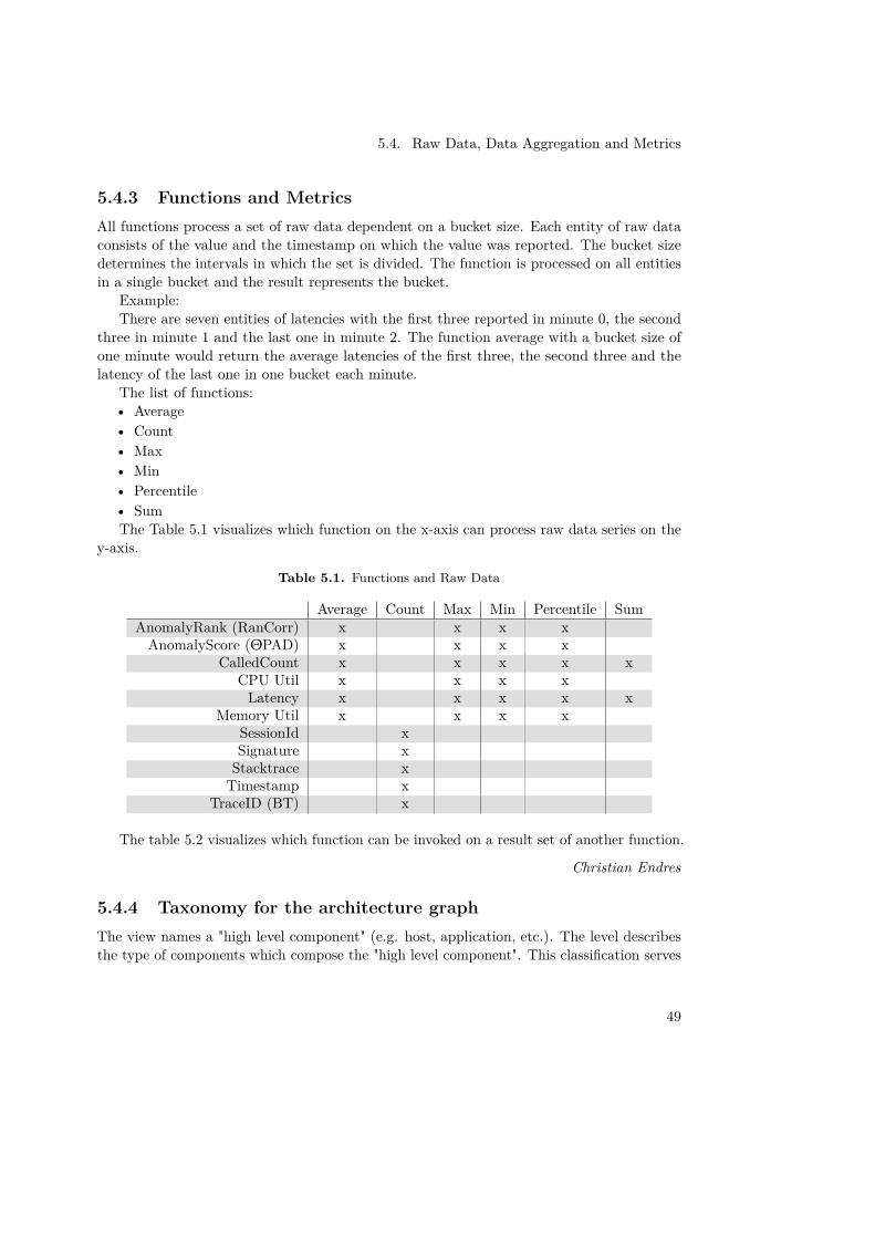
5.4. Raw Data, Data Aggregation and Metrics
5.4.3 Functions and MetricsAll functions process a set of raw data dependent on a bucket size. Each entity of raw dataconsists of the value and the timestamp on which the value was reported. The bucket sizedetermines the intervals in which the set is divided. The function is processed on all entitiesin a single bucket and the result represents the bucket.
Example:There are seven entities of latencies with the first three reported in minute 0, the second
three in minute 1 and the last one in minute 2. The function average with a bucket size ofone minute would return the average latencies of the first three, the second three and thelatency of the last one in one bucket each minute.
The list of functions:• Average• Count• Max• Min• Percentile• SumThe Table 5.1 visualizes which function on the x-axis can process raw data series on the
y-axis.
Table 5.1. Functions and Raw Data
Average Count Max Min Percentile SumAnomalyRank (RanCorr) x x x x
AnomalyScore (ΘPAD) x x x xCalledCount x x x x x
CPU Util x x x xLatency x x x x x
Memory Util x x x xSessionId xSignature x
Stacktrace xTimestamp x
TraceID (BT) x
The table 5.2 visualizes which function can be invoked on a result set of another function.
Christian Endres
5.4.4 Taxonomy for the architecture graphThe view names a "high level component" (e.g. host, application, etc.). The level describesthe type of components which compose the "high level component". This classification serves
49
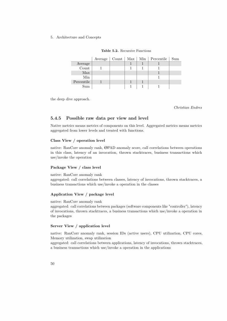
5. Architecture and Concepts
Table 5.2. Recursive Functions
Average Count Max Min Percentile SumAverage 1 1 1
Count 1 1 1 1Max 1Min 1
Percentile 1 1 1Sum 1 1 1
the deep dive approach.
Christian Endres
5.4.5 Possible raw data per view and levelNative metrics means metrics of components on this level. Aggregated metrics means metricsaggregated from lower levels and treated with functions.
Class View / operation level
native: RanCorr anomaly rank, ΘPAD anomaly score, call correlations between operationsin this class, latency of an invocation, thrown stacktraces, business transactions whichuse/invoke the operation
Package View / class level
native: RanCorr anomaly rankaggregated: call correlations between classes, latency of invocations, thrown stacktraces, abusiness transactions which use/invoke a operation in the classes
Application View / package level
native: RanCorr anomaly rankaggregated: call correlations between packages (software components like "controller"), latencyof invocations, thrown stacktraces, a business transactions which use/invoke a operation inthe packages
Server View / application level
native: RanCorr anomaly rank, session IDs (active users), CPU utilization, CPU cores,Memory utilization, swap utilizationaggregated: call correlations between applications, latency of invocations, thrown stacktraces,a business transactions which use/invoke a operation in the applications
50
5.4. Raw Data, Data Aggregation and Metrics
Architecture View / host level
native: RanCorr anomaly rankaggregated: call correlations between hosts, latency of invocations, thrown stacktraces,business transactions which use/invoke an operation in the hosts, session IDs (active users)
Christian Endres
5.4.6 Default metricsArchitecture view: Error Rate, Active UsersServer View : CPU Load, Memory Load, SWAP, Error Rate, RanCorr RankApplication View: RanCorr Rank, Error RatePackage View: RanCorr Rank, Error RateClass View: RanCorr Rank, Error RateOperation View: Average Latency of invocation, Error Rate, Called Count
Panel: Thrown Stacktraces
Anton Scherer
51

Chapter 6
Current state
This chapter describes the state of Kieker and its WebGUI.
6.1 Kieker BackendThis section describes the state of Kieker before the project. The focus lies on properties ofKieker that are modified by Kiekeriki-Backend.
6.1.1 KiekerThe current stable version of Kieker is 1.8. It can be downloaded from the homepage ofKieker1. It is also available via Maven and Git.Detailed information can be found in the documentation section of the Kieker homepage2.Some general information, about aspects of Kieker concerning this project, are provided inthe following sections.
6.1.2 ConfigurationAny implementation of AbstractFilterPlugin can be configured during the construction of thepipes and filter structure.The @Property annotation within the @Plugin annotation allows to define plugin specificproperties including a default value. A Configuration item is mandatory to construct aplugin. The logic to use the configuration is implemented with every AbstractFilterPluginsubclass.After the controller is started with its run() method, there is no way to modify the currentconfiguration of any plugin already constructed.
6.1.3 AnalysisKiekers analysis component consists mainly of the possibility to construct a pipes-and-filterarchitecture composed of various readers and filters. Readers and filters are all registered to
1http://Kieker-monitoring.net/download2http://Kieker-monitoring.net/documentation/
53
6. Current state
and connected by an instance of IAnalysisController. Readers mark the ”beginning” of anypipes-and-filters structure. Every filter to be used needs to be associated with a controller.The connections within any structure are realized through the annotations. The @InputPortis set to a method that receives incoming messages. The @OutputPort annotation is setwithin @Plugin and defines Outputports to which other plugins can connect. The connectionis ensured by the controller.Every new plugin has to be instantiated seperately and then connected by the controller toform a pipes-and-filters-structure. There is no way of predefining ”substructures”.
6.1.4 ΘPADΘPAD, introduced in 2.1, is provided by the opad-tslib-integration branch of the officialKieker git repository. ΘPAD is provided via its corresponding classes. How ΘPAD can beused is shown by the ΘPADx-Demo which can be downloaded from the Kieker wiki3.
6.1.5 RanCorrRanCorr, see 2.1.2, is currently not supported in any way by Kieker.
Markus Fischer
6.2 Kieker FrontendThe Kieker WebGUI which should be enhanced is the stable version 1.8 4. The enhancementdoes not need all functionality provided by the original implementation. Thus the followingclasses or packages are deleted:
• kieker.webgui.web.beans.view.CockpitBean.java• kieker.webgui.web.beans.view.CockpitEditorBean.java• kieker.webgui.web.utility.CockpitLayout.java• java.main.webapp.pages.CockpitEditorPage.xhtml• java.main.webapp.pages.CockpitPage.xhtml• java.main.webapp.pages.ControllerPage.xhtml• java.main.webapp.dialogs.CockpitEditorPageDialogs.xhtml• java.main.webapp.dialogs.ControllerPageDialogs.xhtml• java.main.webapp.css.CockpitEditorPage.css• java.main.webapp.css.CockpitPage.css• java.main.webapp.css.ControllerPage.css
The following classes are edited, because they use deleted classes:3https://Kieker.uni-kiel.de/trac/wiki/opad4https://sourceforge.net/projects/kieker/files/kieker/kieker-1.8/kieker-1.8_sources.zip/download
54
6.2. Kieker Frontend
• kieker.webgui.common:removed unused annotations
• kieker.webgui.common:removed most of converters (except getSuitableAnnotation and function isProgram-maticOnly)
• kieker.webgui.service.IProjectService:removed everything which is related to cockpit
• kieker.webgui.service.impl.ProjectService:removed everything which is related to cockpit
• kieker.webgui.web.beans.applicaton.GlobalProperties.Bean.java:Removed everything related to deleted exceptions
• kieker.webgui.web.beans.view.ControllerBean.java:removed everything related to cockpit
• java.main.webapp.WEB-INFO.faces-config.xml:Removed all unused pages
• java.main.webapp.templates.PagesTemplate.xhtml:Removed all buttons and dialogs related to cockpit
• java.main.webapp.dialogs.SettingsDialog.xhtml:Removed all buttons and dialogues related to cockpit
Martin Scholz, Christian Endres
55

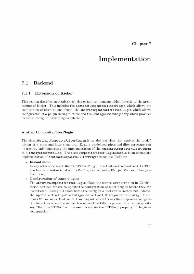
Chapter 7
Implementation
7.1 Backend
7.1.1 Extension of Kieker
This section describes new (abstract) classes and components added directly to the archi-tecture of Kieker. This includes the AbstractCompositeFilterPlugin which allows thecomposition of filters to one plugin, the AbstractUpdateableFilterPlugin which allowsconfiguration of a plugin during runtime and the ConfigurationRegistry which providesmeans to configure Kiekerplugins externally.
AbstractCompositeFilterPlugin
The class AbstractCompositeFilterPlugin is an abstract class that enables the predef-inition of a pipes-and-filter structure. E. g., a predefined pipes-and-filter structure canbe used by only connecting the implementation of the AbstractCompositeFilterPluginto a IAnalysisController. The class CompositeFilterPluginExample is an exemplaryimplementation of AbstractCompositeFilterPlugin using one TeeFilter.
• InstantiationAs any other subclass of AbstractFilterPlugin, the AbstractCompositeFilterPlu-gin has to be instantiated with a Configuration and a IProjectContext (Analysis-Controller).
• Configuration of inner pluginsThe AbstractCompositeFilterPlugin allows the user to write entries in its Configu-ration destined for use to update the configuration of inner plugins before they areinstantiated. Listing 7.1 shows how a the config for a TeeFilter is created and updated.the update method updateConfiguration(final Configuration config, finalClass<? extends AbstractFilterPlugin> clazz) scans the composites configura-tion for entries where the simple class name of TeeFilter is present. E. g., an entry withkey ”TeeFilter.STDlog” will be used to update the ”STDlog” property of the givenconfiguration.
57
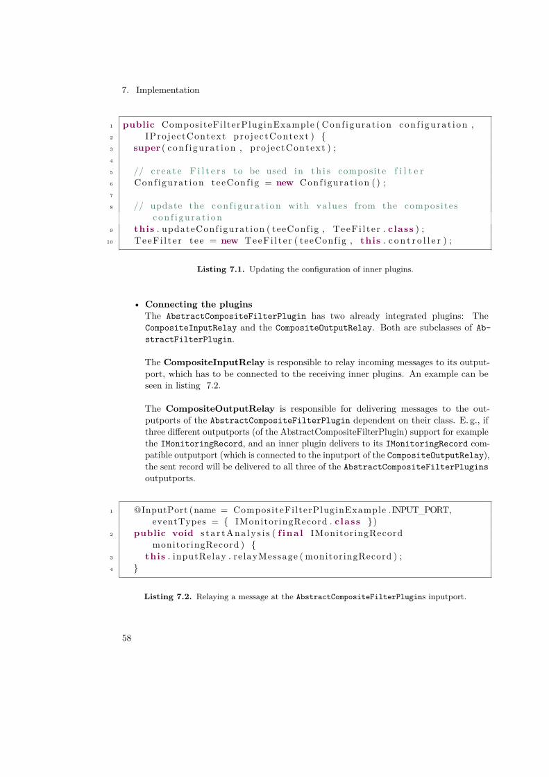
7. Implementation
1 public CompositeFi lterPluginExample ( Conf igurat ion con f i gu ra t i on ,2 IPro jectContext pro jectContext ) {3 super ( con f i gu ra t i on , pro jec tContext ) ;4
5 // c r e a t e F i l t e r s to be used in t h i s composite f i l t e r6 Conf igurat ion teeConf ig = new Conf igurat ion ( ) ;7
8 // update the c o n f i g u r a t i o n with va lue s from the compos i tesc o n f i g u r a t i o n
9 this . updateConf igurat ion ( teeConf ig , TeeF i l t e r . class ) ;10 TeeF i l t e r t e e = new TeeF i l t e r ( teeConf ig , this . c o n t r o l l e r ) ;
Listing 7.1. Updating the configuration of inner plugins.
• Connecting the pluginsThe AbstractCompositeFilterPlugin has two already integrated plugins: TheCompositeInputRelay and the CompositeOutputRelay. Both are subclasses of Ab-stractFilterPlugin.
The CompositeInputRelay is responsible to relay incoming messages to its output-port, which has to be connected to the receiving inner plugins. An example can beseen in listing 7.2.
The CompositeOutputRelay is responsible for delivering messages to the out-putports of the AbstractCompositeFilterPlugin dependent on their class. E. g., ifthree different outputports (of the AbstractCompositeFilterPlugin) support for examplethe IMonitoringRecord, and an inner plugin delivers to its IMonitoringRecord com-patible outputport (which is connected to the inputport of the CompositeOutputRelay),the sent record will be delivered to all three of the AbstractCompositeFilterPluginsoutputports.
1 @InputPort (name = CompositeFi lterPluginExample .INPUT_PORT,eventTypes = { IMonitoringRecord . class })
2 public void s t a r t A n a l y s i s ( f ina l IMonitor ingRecordmonitoringRecord ) {
3 this . inputRelay . re layMessage ( monitoringRecord ) ;4 }
Listing 7.2. Relaying a message at the AbstractCompositeFilterPlugins inputport.
58

7.1. Backend
The inner plugins can be connected in the Kieker customary fashion. Important is thatall plugins that need input from outside the AbstractCompositeFilterPlugin areconnected to the CompositeInputRelay and that all plugins that want to deliver outsideof the AbstractCompositeFilterPlugin are connected to the CompositeOutputRelay.Example 7.3 shows a connection from the CompositeInputRelay to a TeeFilter to theCompositeOutputRelay.
1 // connect InputRelay to TeeF i l t e r2 this . c o n t r o l l e r . connect ( inputRelay , CompositeInputRelay .
INPUTRELAY_OUTPUTPORT, tee , TeeF i l t e r .INPUT_PORT_NAME_EVENTS);
3 // connect TeeF i l t e r to OutputRelay4 this . c o n t r o l l e r . connect ( tee , TeeF i l t e r .
OUTPUT_PORT_NAME_RELAYED_EVENTS, outputRelay ,CompositeOutputRelay .INPUT_PORT_NAME_EVENTS) ;
Listing 7.3. Example of connecting the plugins within the AbstractCompositePluginFilter.
• Limitations– Currently it is only possible to receive Messages of class IMonitoringRecord since
the CompositeInputRelay only supports this inputport.– Inner plugins of the same class can not be configured with different values for the
same properties when using the updateConfiguration(...) method
Markus Fischer
AbstractUpdateableFilterPlugin
The class AbstractUpdateableFilterPLugin is an abstract class to enable the runtime con-figuration of any plugin. The AbstractUpdateableFilterPLugin extends the AbstractFil-terPlugin. The class UpdateableFilterPluginExample is an exemplary implementation.
• PropertiesListing 7.4 show how properties can be declared ”updateable = true”. The defaultvalue is false. The boolean marks if a property is generally updateable during runtime.
• Method setCurrentConfiguration(...)The abstract method setCurrentConfiguration(...) is designated to update aplugins configuration during runtime. The boolean ”update” marks whether all prop-erties are updated (update = false) or only the properties marked as updateable arereconfigured. An exemplary implementation is shown in listing 7.5.
• Usage To reconfigure plugins during runtime they have to be registered to a Configu-rationRegistry, see 7.1.1
59
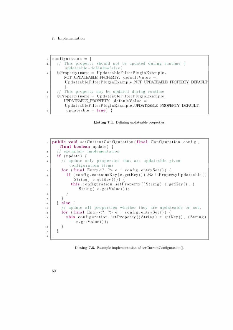
7. Implementation
1 c o n f i g u r a t i o n = {2 // This property should not be updated during runtime (
updateable�d e f a u l t=f a l s e )3 @Property (name = UpdateableFi l terPluginExample .
NOT_UPDATEABLE_PROPERTY, de fau l tVa lue =UpdateableFi l terPluginExample .NOT_UPDATEABLE_PROPERTY_DEFAULT) ,
4 // This property may be updated during runtime5 @Property (name = UpdateableFi l terPluginExample .
UPDATEABLE_PROPERTY, de fau l tVa lue =UpdateableFi l terPluginExample .UPDATEABLE_PROPERTY_DEFAULT,
6 updateable = true ) }
Listing 7.4. Defining updateable properties.
1 public void s e tCurrentConf i gura t i on ( f ina l Conf igurat ion con f i g ,f ina l boolean update ) {
2 // exemplary implementation3 i f ( update ) {4 // update only p r o p e r t i e s that are updateable g iven
c o n f i g u r a t i o n items5 for ( f ina l Entry <?, ?> e : c o n f i g . entrySet ( ) ) {6 i f ( c o n f i g . containsKey ( e . getKey ( ) ) && isPropertyUpdateable ( (
S t r ing ) e . getKey ( ) ) ) {7 this . c o n f i g u r a t i o n . se tProper ty ( ( S t r ing ) e . getKey ( ) , (
S t r ing ) e . getValue ( ) ) ;8 }9 }
10 } else {11 // update a l l p r o p e r t i e s whether they are updateable or not .12 for ( f ina l Entry <?, ?> e : c o n f i g . entrySet ( ) ) {13 this . c o n f i g u r a t i o n . se tProper ty ( ( S t r ing ) e . getKey ( ) , ( S t r ing )
e . getValue ( ) ) ;14 }15 }16 }
Listing 7.5. Example implementation of setCurrentConfiguration().
60

7.1. Backend
Markus Fischer
ConfigurationRegistry
The ConfigurationRegistry provides functionality to register instances of AbstractUp-dateableFilterPlugin and update their configuration during runtime.The ConfigurationRegistry consists of the abstract class AbstractConfigurationRegistry,the interface IConfigurationRegistry and the GlobalConfigurationRegistry which is asingleton.
• Register a pluginAny AbstractUpdateableFilterPlugin can be registered to a ConfigurationRegistry.The GlobalConfigurationRegistry provides a globally visible and usable Configura-tionRegistry within Kieker. To register a plugin it needs a globally (within the scopeof Kieker) unique String identifier, see example listing 7.6.
1 // r e g i s t e r a p lug in2 Globa lCon f i gura t i onReg i s t ry . g e t In s tance ( ) .
r e g i s t e r U p d a t e a b l e F i l t e r P l u g i n ( " uniqueID " , updateablePlug in ) ;3
4 // update a p lug in5 Conf igurat ion conf = new Conf igurat ion ( ) ;6 conf . s e tProper ty ( " propertyName " , " newValue " ) ;7 Globa lCon f i gura t i onReg i s t ry . g e t In s tance ( ) . updateConf igurat ion ( "
uniqueID " , conf , true ) ;
Listing 7.6. Using the GlobalCongigurationRegistry.
• Update a pluginAll registered plugins can be retrieved using the GlobalCongigurationRegistry. Anexample is shown in listing 7.6.If the given id is not present in the registry a PluginNotFoundException is thrown.
Markus Fischer
7.1.2 Implementation of RanCorrThis section describes the implementation of RanCorr (see chapter 2.1.2) in Kiekeriki. Inthe following sections this implementation is just called RanCorr.
Architecture Data Model
RanCorr needs its own data model because the data model of Kieker doesn’t provide enoughinformation about the monitored architecture and the calculated anomaly scores. Figure
61

7. Implementation
7.1 shows the developed architecture data model. There is the abstract class Abstrac-tRanCorrItem which represents any architecture component monitored by Kiekeriki. Theimplemented classes based on AbstractRanCorrItem are:
• RanCorrHost represents the host of the monitored system and decorates the classExecutionContainer by Kieker. A host may contain several applications.
• RanCorrApplication represents the application which is monitored. This is a newcomponent and was not considered by the original version of Kieker. An applicationmay contain several packages.
• RanCorrPackage represents a Java package in the monitored application. Also thepackage is not in the original Kieker data model. Kieker knows packages only throughthe monitored operations which contain a package path. A package may contain severalsub packages and classes.
• RanCorrClass represents a Java class and decorates the class ComponentType by Kieker.A class may contain several operations.
• RanCorrOperation represents a Java method and decorates the class Operation byKieker. It may contain several anomaly scores and the calling dependencies to otheroperations.
Input/Output Model
The RanCorr algorithms, described detailed in the paragraphs below, need the class RanCor-rInput as input, which contains the monitored operations with the according anomaly scores(see Figure 7.2). The input object also contains a reference to the class DependencyManagerwhich contains the information about the calling dependencies of operations and the accordingweights. The RanCorr algorithm creates objects of the class RanCorrOutput which containthe mapping between architecture items and the calculated anomaly rankings. Additionallythe output contains the information which algorithm was used to calculate the anomalyranking, indicated by the enumeration RanCorrAlgorithmEnum. The RanCorrInput containsanomaly scores in range [-1.0, 1.0]. The RanCorrOutput contains anomaly rankings in range[0.0, 1.0].
Dependency Handling
The calling dependency handling is actually not considered in Kieker. Hence each RanCorrOp-eration contains direct references to operations which call this RanCorrOperation and arecalled by this RanCorrOperation. Additionally the class DependencyManager contains everydependency information as triple of two RanCorrOperation objects and the according weight.This information is used by the advanced RanCorr algorithm to prioritize the dependencies.
62
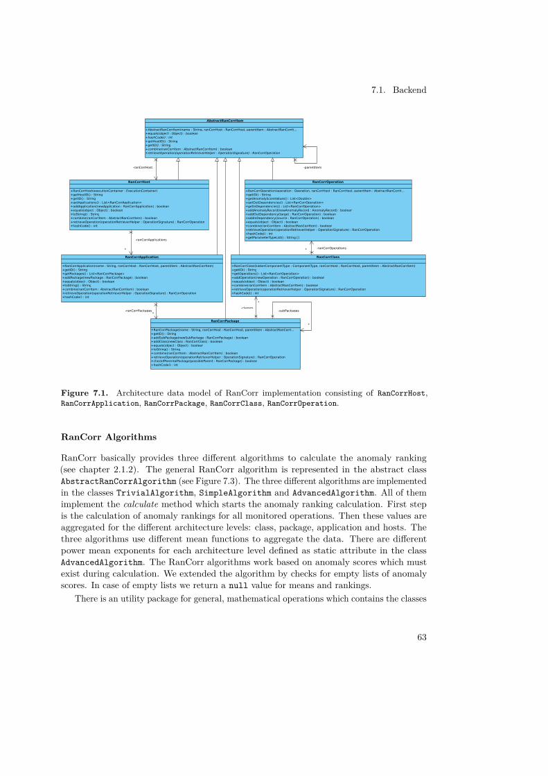
7.1. Backend
+AbstractRanCorrItem(name : String, ranCorrHost : RanCorrHost, parentItem : AbstractRanCorrIt...+equals(object : Object) : boolean+hashCode() : int+getHostID() : String+getID() : String+combine(ranCorrItem : AbstractRanCorrItem) : boolean+retrieveOperation(operationRetrieverHelper : OperationSignature) : RanCorrOperation
AbstractRanCorrItem
+RanCorrApplication(name : String, ranCorrHost : RanCorrHost, parentItem : AbstractRanCorrItem)+getID() : String+getPackages() : List<RanCorrPackage>+addPackage(newPackage : RanCorrPackage) : boolean+equals(object : Object) : boolean+toString() : String+combine(ranCorrItem : AbstractRanCorrItem) : boolean+retrieveOperation(operationRetrieverHelper : OperationSignature) : RanCorrOperation+hashCode() : int
RanCorrApplication
+RanCorrClass(kiekerComponentType : ComponentType, ranCorrHost : RanCorrHost, parentItem : AbstractRanCorrItem)+getID() : String+getOperations() : List<RanCorrOperation>+addOperation(newOperation : RanCorrOperation) : boolean+equals(object : Object) : boolean+combine(ranCorrItem : AbstractRanCorrItem) : boolean+retrieveOperation(operationRetrieverHelper : OperationSignature) : RanCorrOperation+hashCode() : int
RanCorrClass
+RanCorrHost(executionContainer : ExecutionContainer)+getHostID() : String+getID() : String+getApplications() : List<RanCorrApplication>+addApplication(newApplication : RanCorrApplication) : boolean+equals(object : Object) : boolean+toString() : String+combine(ranCorrItem : AbstractRanCorrItem) : boolean+retrieveOperation(operationRetrieverHelper : OperationSignature) : RanCorrOperation+hashCode() : int
RanCorrHost
+RanCorrOperation(operation : Operation, ranCorrHost : RanCorrHost, parentItem : AbstractRanCorrIt...+getID() : String+getAnomalyScoreValues() : List<Double>+getOutDependencies() : List<RanCorrOperation>+getInDependencies() : List<RanCorrOperation>+addAnomalyRecord(newAnomalyRecord : AnomalyRecord) : boolean+addOutDependency(target : RanCorrOperation) : boolean+addInDependency(source : RanCorrOperation) : boolean+equals(object : Object) : boolean+combine(ranCorrItem : AbstractRanCorrItem) : boolean+retrieveOperation(operationRetrieverHelper : OperationSignature) : RanCorrOperation+hashCode() : int+getParameterTypeList() : String []
RanCorrOperation
+RanCorrPackage(name : String, ranCorrHost : RanCorrHost, parentItem : AbstractRanCorrI...+getID() : String+addSubPackage(newSubPackage : RanCorrPackage) : boolean+addClass(newClass : RanCorrClass) : boolean+equals(object : Object) : boolean+toString() : String+combine(ranCorrItem : AbstractRanCorrItem) : boolean+retrieveOperation(operationRetrieverHelper : OperationSignature) : RanCorrOperation+checkIfParentalPackage(possibleParent : RanCorrPackage) : boolean+hashCode() : int
RanCorrPackage
-ranCorrHost
-classes
*
-ranCorrApplications
* -ranCorrOperations*
-ranCorrPackages*
-parentItem
-subPackages
*
Figure 7.1. Architecture data model of RanCorr implementation consisting of RanCorrHost,RanCorrApplication, RanCorrPackage, RanCorrClass, RanCorrOperation.
RanCorr Algorithms
RanCorr basically provides three different algorithms to calculate the anomaly ranking(see chapter 2.1.2). The general RanCorr algorithm is represented in the abstract classAbstractRanCorrAlgorithm (see Figure 7.3). The three different algorithms are implementedin the classes TrivialAlgorithm, SimpleAlgorithm and AdvancedAlgorithm. All of themimplement the calculate method which starts the anomaly ranking calculation. First stepis the calculation of anomaly rankings for all monitored operations. Then these values areaggregated for the different architecture levels: class, package, application and hosts. Thethree algorithms use different mean functions to aggregate the data. There are differentpower mean exponents for each architecture level defined as static attribute in the classAdvancedAlgorithm. The RanCorr algorithms work based on anomaly scores which mustexist during calculation. We extended the algorithm by checks for empty lists of anomalyscores. In case of empty lists we return a null value for means and rankings.
There is an utility package for general, mathematical operations which contains the classes
63
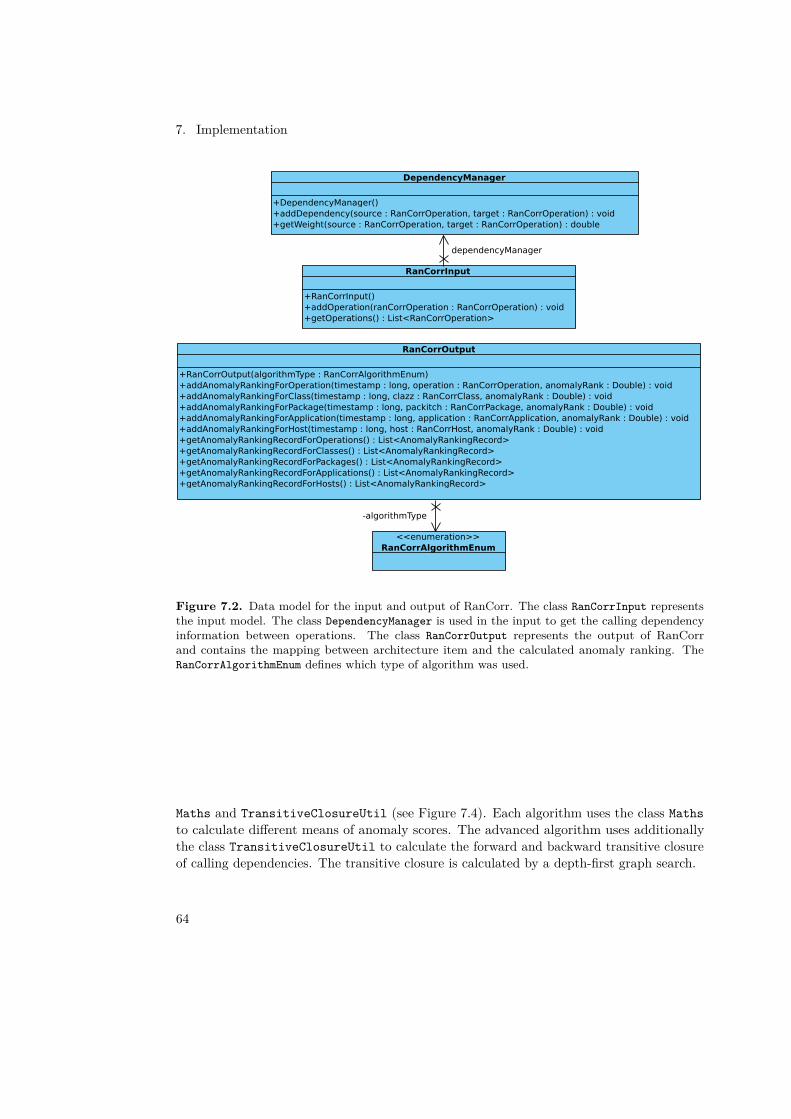
7. Implementation
+RanCorrInput()+addOperation(ranCorrOperation : RanCorrOperation) : void+getOperations() : List<RanCorrOperation>
RanCorrInput
+RanCorrOutput(algorithmType : RanCorrAlgorithmEnum)+addAnomalyRankingForOperation(timestamp : long, operation : RanCorrOperation, anomalyRank : Double) : void+addAnomalyRankingForClass(timestamp : long, clazz : RanCorrClass, anomalyRank : Double) : void+addAnomalyRankingForPackage(timestamp : long, packitch : RanCorrPackage, anomalyRank : Double) : void+addAnomalyRankingForApplication(timestamp : long, application : RanCorrApplication, anomalyRank : Double) : void+addAnomalyRankingForHost(timestamp : long, host : RanCorrHost, anomalyRank : Double) : void+getAnomalyRankingRecordForOperations() : List<AnomalyRankingRecord>+getAnomalyRankingRecordForClasses() : List<AnomalyRankingRecord>+getAnomalyRankingRecordForPackages() : List<AnomalyRankingRecord>+getAnomalyRankingRecordForApplications() : List<AnomalyRankingRecord>+getAnomalyRankingRecordForHosts() : List<AnomalyRankingRecord>
RanCorrOutput
<<enumeration>>RanCorrAlgorithmEnum
+DependencyManager()+addDependency(source : RanCorrOperation, target : RanCorrOperation) : void+getWeight(source : RanCorrOperation, target : RanCorrOperation) : double
DependencyManager
dependencyManager
-algorithmType
Figure 7.2. Data model for the input and output of RanCorr. The class RanCorrInput representsthe input model. The class DependencyManager is used in the input to get the calling dependencyinformation between operations. The class RanCorrOutput represents the output of RanCorrand contains the mapping between architecture item and the calculated anomaly ranking. TheRanCorrAlgorithmEnum defines which type of algorithm was used.
Maths and TransitiveClosureUtil (see Figure 7.4). Each algorithm uses the class Mathsto calculate different means of anomaly scores. The advanced algorithm uses additionallythe class TransitiveClosureUtil to calculate the forward and backward transitive closureof calling dependencies. The transitive closure is calculated by a depth-first graph search.
64

7.1. Backend
+calculate(input : RanCorrInput) : RanCorrOutput+mapToPropabilityRange(anomalyRanking : Double) : Double
AbstractRanCorrAlgorithm(kieker::tools::rancorr::algorithms)
+AdvancedAlgorithm()+calculate(input : RanCorrInput) : RanCorrOutput
AdvancedAlgorithm(kieker::tools::rancorr::algorithms)
+SimpleAlgorithm()+calculate(input : RanCorrInput) : RanCorrOutput
SimpleAlgorithm(kieker::tools::rancorr::algorithms)
+TrivialAlgorithm()+calculate(input : RanCorrInput) : RanCorrOutput
TrivialAlgorithm(kieker::tools::rancorr::algorithms)
<<Constant>> TRIVIAL<<Constant>> SIMPLE<<Constant>> ADVANCED
<<enumeration>><<Enum>>
RanCorrAlgorithmEnum(kieker::tools::rancorr)
Figure 7.3. The three types of RanCorr algorithms are implemented in the classes TrivialAlgo-rithm, SimpleAlgorithm and AdvancedAlgorithm which all extend the abstract class AbstractRan-CorrAlgorithm. The enumeration RanCorrAlgorithmEnum can be used to identify them.
+gamma(a : double, q : double) : double+unweightedArithmeticMean(values : List<Double>) : Double+unweightedPowerMean(values : List<Double>, p : double) : Double+weightedPowerMean(values : List<Double>, weights : List<Double>, p : double) : Double
Maths
+forwardTransitiveClosure(source : RanCorrOperation) : Set<RanCorrOperation>+backwardTransitiveClosure(dependencyManager : DependencyManager, target : RanCorrOperation, distance : double, weight : double) : Map<RanCorrOperation, PathRecord>+mergeClosure(closure : Map<RanCorrOperation, PathRecord>, newItem : RanCorrOperation, newDistance : double, newWeight : double) : Map<RanCorrOperation, PathRecord>+mergeClosure(closure1 : Map<RanCorrOperation, PathRecord>, closure2 : Map<RanCorrOperation, PathRecord>) : Map<RanCorrOperation, PathRecord>
TransitiveClosureUtil
Figure 7.4. The RanCorr algorithms use the util classes to calculate the anomaly rankings. The classMaths contains math functions to calculate different means and the class TransitiveClosureUtilcontains functions to calculate transitive closures of calling dependencies.
Integration into Kieker
In order to integrate RanCorr in the Kieker framework we built a new filter which starts theRanCorr calculation. The class RanCorrFilter represents that filter (see Figure 7.5). Thisfilter has two input ports: one for the objects of class MessageTrace and one for objectsof class OperationAnomalyInfo. The first port is used to read the message traces and torebuild the architecture model of the monitored system. We achieve this by using the methodconvert of the class RanCorrInputProvider. This method analyze the messages in the givenmessage trace and rebuilds the architecture with all elements. Finally it returns an object ofthe class RanCorrInput with which the RanCorr algorithm is started. The second port isused to get the anomaly score information for the several operations. This will be typicallythe output of ΘPADx. The range of that input values should be in range [0.0, 1.0]. Thetype of the used RanCorr algorithm can be configured via the filter configuration. There isalso an additional filter represented by the class RanCorrOutputDBWriter which is used towrite the results of RanCorr in the exchange database. This filter has one input port for
65
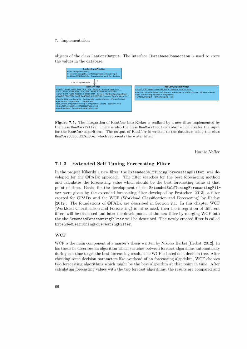
7. Implementation
objects of the class RanCorrOutput. The interface IDatabaseConnection is used to storethe values in the database.
+RanCorrInputProvider()+convert(messageTrace : MessageTrace) : RanCorrInput+addNewOPADData(info : OperationAnomalyInfo) : boolean
RanCorrInputProvider
+OUTPUT_PORT_NAME_RANCORR_DATA : String = "RanCorrOutputData"+INPUT_PORT_NAME_RANCORR_DATA : String = "RanCorrInputData"+INPUT_PORT_NAME_RANCORR_OPAD_DATA : String = "RanCorrOpadInputData"+CONFIG_PROPERTY_NAME_RANCORR_ALGORITHM : String = "RanCorrAlgorithm"
+RanCorrFilter(configuration : Configuration, projectContext : IProjectContext)+getCurrentConfiguration() : Configuration+setCurrentConfiguration(config : Configuration, update : boolean) : void+execute(messageTrace : MessageTrace) : void+opadInput(info : OperationAnomalyInfo) : void
RanCorrFilter
+INPUT_PORT_NAME_RANCORR_DATA : String = "RanCorrData"
+RanCorrOutputDBWriter(configuration : Configuration, projectContext : IProjectContext)+getCurrentConfiguration() : Configuration+writeToDB(output : RanCorrOutput) : void
RanCorrOutputDBWriter
-ranCorrInputProvider1
Figure 7.5. The integration of RanCorr into Kieker is realized by a new filter implemented bythe class RanCorrFilter. There is also the class RanCorrInputProvider which creates the inputfor the RanCorr algorithms. The output of RanCorr is written to the database using the classRanCorrOutputDBWriter which represents the writer filter.
Yannic Noller
7.1.3 Extended Self Tuning Forecasting FilterIn the project Kikeriki a new filter, the ExtendedSelfTuningForecastingFilter, was de-veloped for the ΘPADx approach. The filter searches for the best forecasting methodand calculates the forecasting value which should be the best forecasting value at thatpoint of time. Basics for the development of the ExtendedSelfTuningForecastingFil-ter were given by the extended forecasting filter developed by Frotscher [2013], a filtercreated for ΘPADx and the WCF (Workload Classification and Forecasting) by Herbst[2012]. The foundations of ΘPADx are described in Section 2.1. In this chapter WCF(Workload Classification and Forecasting) is introduced, then the integration of differentfilters will be discussed and later the development of the new filter by merging WCF intothe the ExtendedForecastingFilter will be described. The newly created filter is calledExtendedSelfTuningForecastingFilter.
WCF
WCF is the main component of a master’s thesis written by Nikolas Herbst [Herbst, 2012]. Inhis thesis he describes an algorithm which switches between forecast algorithms automaticallyduring run-time to get the best forecasting result. The WCF is based on a decision tree. Afterchecking some decision parameters like overhead of an forecasting algorithm, WCF choosestwo forecasting algorithms which might be the best algorithm at that point in time. Aftercalculating forecasting values with the two forecast algorithms, the results are compared and
66

7.1. Backend
the better result is chosen by WCF. For a deeper understanding of WCF it is recommendedto read Herbst’s thesis [Herbst, 2012].
An advantage of using WCF in Kikeriki is, there is an implementation which couldbe used in our project. The requirement of the project to be able to choose the bestforecast algorithm during run-time could be solved with the approach of Herbst’s thesis.Another advantage of using WCF is, that in the WCF implementation were some forecastingalgorithms implemented already, which were not implemented in ΘPADx/Kieker yet. Becausethe algorithm methods were implemented similarly, they could be easily reused within ourproject. As a result the requirement to add more forecasting algorithms into ΘPADx couldbe solved.
Integration of forecasting methods
In ΘPADx there are different forecasting algorithms implemented. During the integration ofWCF more forecasting methods were added. The new added forecasting methods includethe ARIMA, Croston, SES, Naive and TBATS forecasting method. Two forecasting methodsare not in the Extended Self Tuning Forecasting Filter, which were used in the ExtendedForecasting Filter: The SESR and the ARIMA101 forecasting method. The SESR is replacedby the SES forecasting method because the SESR forecasting implementation was not writtenin pure R code. ARIMA101 was replaced by the ARIMA forecasting method because atsome special time series ARIMA101 is not applicable. During testing, we found an errorin the R implementation of ARIMA. So it may occur that the ARIMA forecasting methoddoes not work as expected. Fortunately the WCF algorithm always uses two forecastingmethods so if ARIMA does not work, the second forecasting method is used. Also
Figure 7.6. Forecasting filters
all forecasting methods not implemented in R were replaced by R forecasting methods.Only the Mean forecasting method is, besides the R method, written in Java, is part ofthe ExtendedSelfTuningForecastingFilter which can be used for forecasting. The javamethod should only be used for debugging purposes. The advantage of the Java method is,that the R environment is not needed.
67

7. Implementation
Implementation of the ExtendedSelfTuningForecastingFilter
As mentioned before the ExtendedSelfTuningForecastingFilter is based on the imple-mentation of WCF. The main difference between the original WCF implementation andthe integration of WCF into the new ExtendedSelfTuningForecastingFilter is the dataprocessing. In the approach of Herbst [2012] the input data is read form a xls fil. For theΘPADx filter environment, the data is sent to the forecasting filter whenever data is readby the Kieker reader and send to the ΘPADx filter architecture. A condensed sequencediagram of the ExtendedSelfTuningForecastingFilter is shown in the diagram below.The sequence diagram shows the flow if self-tuning is activated. The mechanic of theExtendedSelfTuningForecastingFilter is shown in the documentation of WCF [Herbst,2012].
Figure 7.7. Sequence diagram of the extended self tuning forecasting filter.
As it can be seen in Figure 7.7 the ExtendedSelfTuningForecastingFilter receivesa Time Series Point (TSP)from another filter as input data. For each TSP received onthe input port of the ExtendedSelfTuningForecastingFilter, a new WorkloadIntensi-tyBehavior (WIB) is created. The created WIB is stored in a ConcurrentHashMap. In thehash map the name of the called function is the key of the hash map. So every function isforecasted on its own. In the listing below the creation of the hash map and the storage ofthe object is shown.
68
7.2. Frontend
1 i f ( this . s e l f t u n i n g b o o l . get ( ) ) {2 . . .3 f ina l WorkloadIntens ityBehavior newWib = new
WorkloadIntens ityBehavior ( . . . ) ;4 this . wibStore . put ( input . getName ( ) , newWib) ;5 }
Listing 7.7. Create WIB object and store the object into the wibStore hashmap.
Next the incoming TSP is added to the time series. With the function callForecaster()the forecasting is started. First of all the time series is classify into a category to find the bestforecasting methods. The possible categories are initial, fast and complex. The procedure isbased on some decision points like length of the time series. How the classification exactlyworks is described in [Herbst, 2012]. Compared to the implementation of Herbst, somedecision points which do not fit into the ΘPADx/Kieker environment are not used in theimplementation of the ExtendedSelfTuningForecastingFilter. Decision points like forexample amount of skipped values are not used anymore. After the classification is finished,the two forecasting methods, which were chosen by the classification function, are called.These two forecasting methods calculate the forecasting value. After the two results havebeen compared, the better result is sent within a ForecastMeasurementPair (FSP) to theExtendedSelfTuningForecastingFilter output port. For the possibility to change betweenself tuning mode and an forecasting method chosen by the user, there is the filter propertyPROPERTY_SELFTUNING_ON implemented. If the boolean property is set to true, the filter runsin self tuning mode. Otherwise the filter can be used as the ExtendedForecastingFilterdeveloped by [Herbst, 2012].
Tobias Rudolph
7.2 FrontendIn this section we present the design and implementation details for the given frontendarchitecture. The components Logic, Web GUI, Cache and the internal database are describedin separate subsection as well as the Transfer Database and the Data Generator which writessynthesized data into the Transfer Database and provides benchmarking functionality.
7.2.1 Web GUIThe Web GUI was developed based on a sketch that was created in the first sprint of thedevelopment project. Ideas for the sketch were based on the evaluated APM Tools currentlyon the market (See chapter 2.4). Figure 7.8 shows the main features the frontend should offerin the main page, the Project View Page. One requirement was to display the aggregated
69
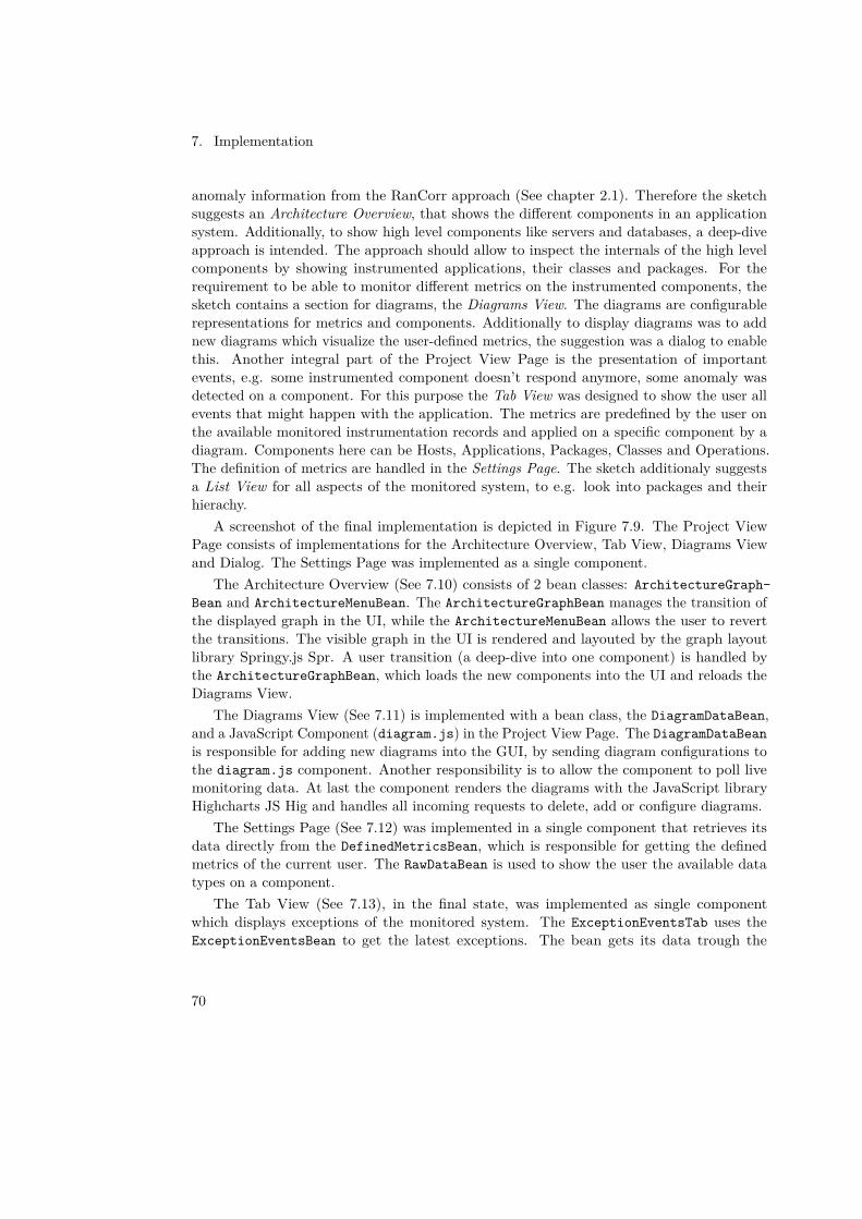
7. Implementation
anomaly information from the RanCorr approach (See chapter 2.1). Therefore the sketchsuggests an Architecture Overview, that shows the different components in an applicationsystem. Additionally, to show high level components like servers and databases, a deep-diveapproach is intended. The approach should allow to inspect the internals of the high levelcomponents by showing instrumented applications, their classes and packages. For therequirement to be able to monitor different metrics on the instrumented components, thesketch contains a section for diagrams, the Diagrams View. The diagrams are configurablerepresentations for metrics and components. Additionally to display diagrams was to addnew diagrams which visualize the user-defined metrics, the suggestion was a dialog to enablethis. Another integral part of the Project View Page is the presentation of importantevents, e.g. some instrumented component doesn’t respond anymore, some anomaly wasdetected on a component. For this purpose the Tab View was designed to show the user allevents that might happen with the application. The metrics are predefined by the user onthe available monitored instrumentation records and applied on a specific component by adiagram. Components here can be Hosts, Applications, Packages, Classes and Operations.The definition of metrics are handled in the Settings Page. The sketch additionaly suggestsa List View for all aspects of the monitored system, to e.g. look into packages and theirhierachy.
A screenshot of the final implementation is depicted in Figure 7.9. The Project ViewPage consists of implementations for the Architecture Overview, Tab View, Diagrams Viewand Dialog. The Settings Page was implemented as a single component.
The Architecture Overview (See 7.10) consists of 2 bean classes: ArchitectureGraph-Bean and ArchitectureMenuBean. The ArchitectureGraphBean manages the transition ofthe displayed graph in the UI, while the ArchitectureMenuBean allows the user to revertthe transitions. The visible graph in the UI is rendered and layouted by the graph layoutlibrary Springy.js Spr. A user transition (a deep-dive into one component) is handled bythe ArchitectureGraphBean, which loads the new components into the UI and reloads theDiagrams View.
The Diagrams View (See 7.11) is implemented with a bean class, the DiagramDataBean,and a JavaScript Component (diagram.js) in the Project View Page. The DiagramDataBeanis responsible for adding new diagrams into the GUI, by sending diagram configurations tothe diagram.js component. Another responsibility is to allow the component to poll livemonitoring data. At last the component renders the diagrams with the JavaScript libraryHighcharts JS Hig and handles all incoming requests to delete, add or configure diagrams.
The Settings Page (See 7.12) was implemented in a single component that retrieves itsdata directly from the DefinedMetricsBean, which is responsible for getting the definedmetrics of the current user. The RawDataBean is used to show the user the available datatypes on a component.
The Tab View (See 7.13), in the final state, was implemented as single componentwhich displays exceptions of the monitored system. The ExceptionEventsTab uses theExceptionEventsBean to get the latest exceptions. The bean gets its data trough the
70
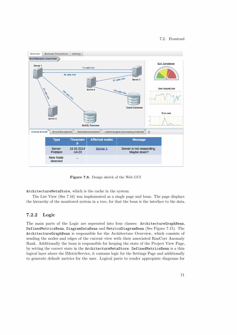
7.2. Frontend
Figure 7.8. Design sketch of the Web GUI
ArchitectureMetaStore, which is the cache in the system.The List View (See 7.16) was implemented as a single page and bean. The page displays
the hierarchy of the monitored system in a tree, for that the bean is the interface to the data.
7.2.2 Logic
The main parts of the Logic are seperated into four classes: ArchitectureGraphBean,DefinedMetricsBean, DiagramDataBean and MetricsDiagramBean (See Figure 7.15). TheArchitectureGraphBean is responsible for the Architecture Overview, which consists ofsending the nodes and edges of the current view with their associated RanCorr AnomalyRank. Additionally the bean is responsible for keeping the state of the Project View Page,by setting the correct state in the ArchitectureMetaStore. DefinedMetricsBean is a thinlogical layer above the IMetricService, it contains logic for the Settings Page and additionallyto generate default metrics for the user. Logical parts to render appropiate diagrams for
71
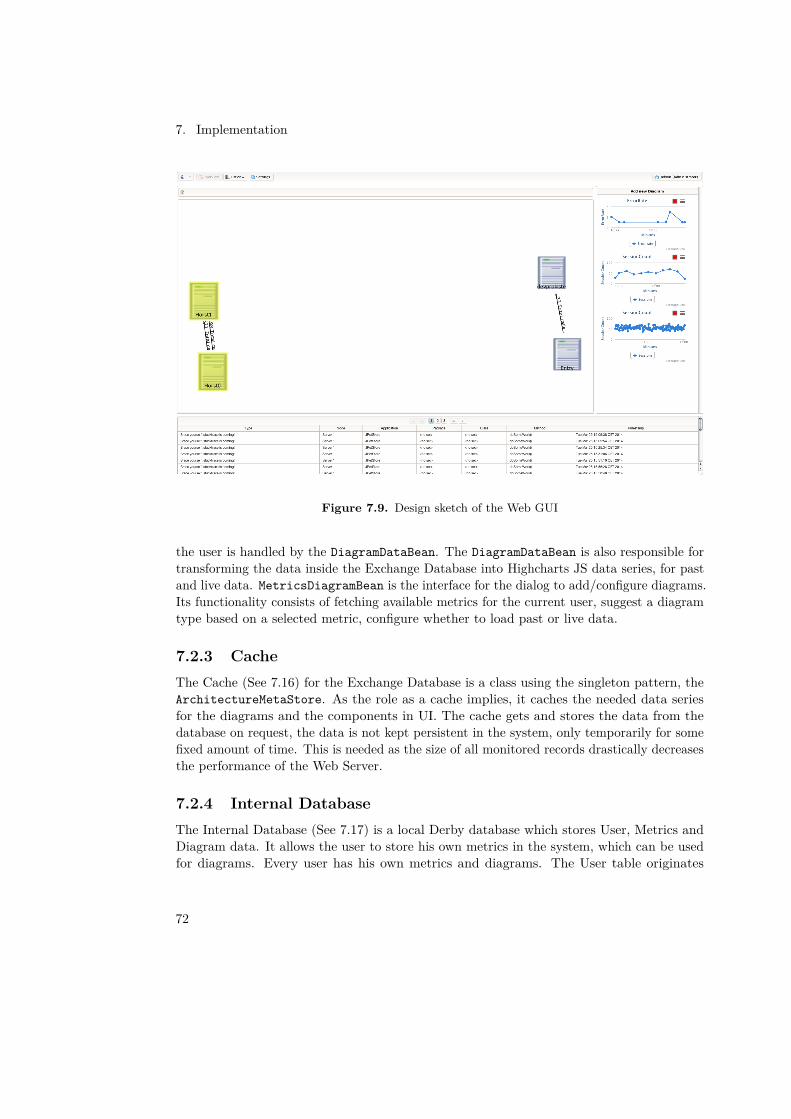
7. Implementation
Figure 7.9. Design sketch of the Web GUI
the user is handled by the DiagramDataBean. The DiagramDataBean is also responsible fortransforming the data inside the Exchange Database into Highcharts JS data series, for pastand live data. MetricsDiagramBean is the interface for the dialog to add/configure diagrams.Its functionality consists of fetching available metrics for the current user, suggest a diagramtype based on a selected metric, configure whether to load past or live data.
7.2.3 CacheThe Cache (See 7.16) for the Exchange Database is a class using the singleton pattern, theArchitectureMetaStore. As the role as a cache implies, it caches the needed data seriesfor the diagrams and the components in UI. The cache gets and stores the data from thedatabase on request, the data is not kept persistent in the system, only temporarily for somefixed amount of time. This is needed as the size of all monitored records drastically decreasesthe performance of the Web Server.
7.2.4 Internal DatabaseThe Internal Database (See 7.17) is a local Derby database which stores User, Metrics andDiagram data. It allows the user to store his own metrics in the system, which can be usedfor diagrams. Every user has his own metrics and diagrams. The User table originates
72
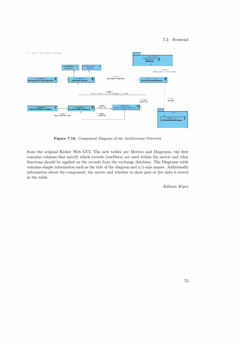
7.2. Frontend
Figure 7.10. Component Diagram of the Architecture Overview
from the original Kieker Web GUI. The new tables are Metrics and Diagrams, the firstcontains columns that specify which records (rawData) are used within the metric and whatfunctions should be applied on the records from the exchange database. The Diagrams tablecontains simple information such as the title of the diagram and x/y-axis names. Additionallyinformation about the component, the metric and whether to show past or live data is storedin the table.
Kálmán Képes
73
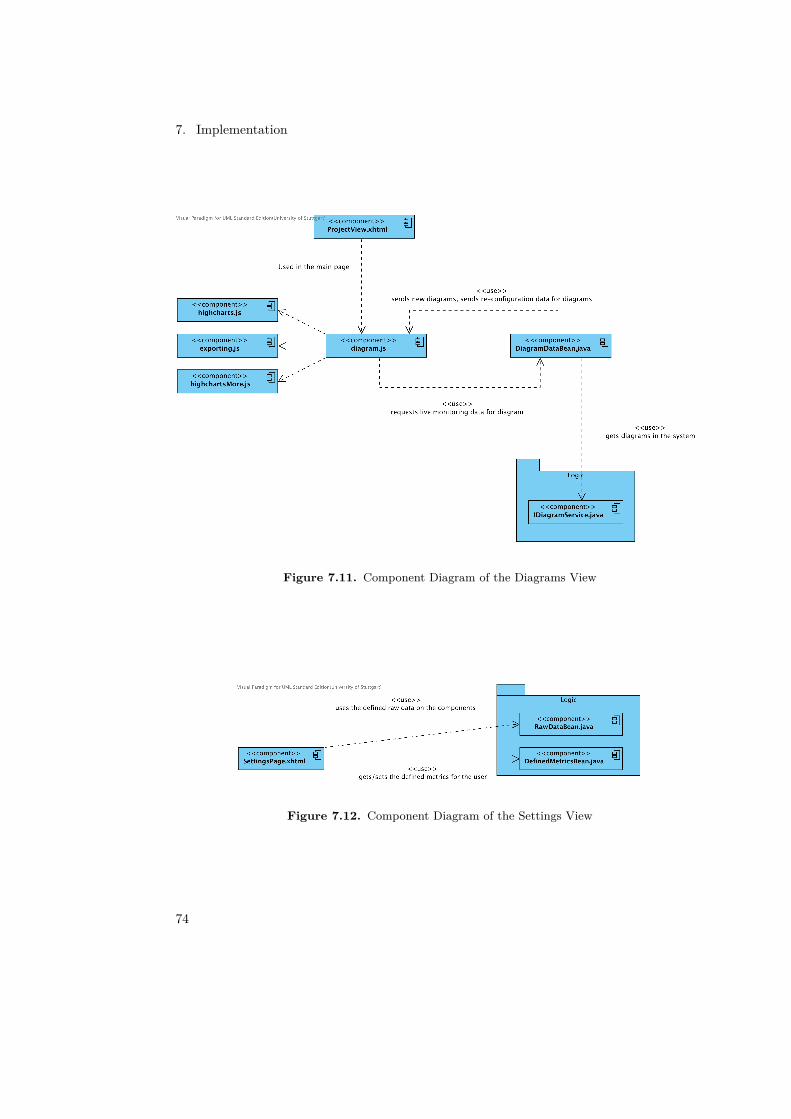
7. Implementation
Figure 7.11. Component Diagram of the Diagrams View
Figure 7.12. Component Diagram of the Settings View
74
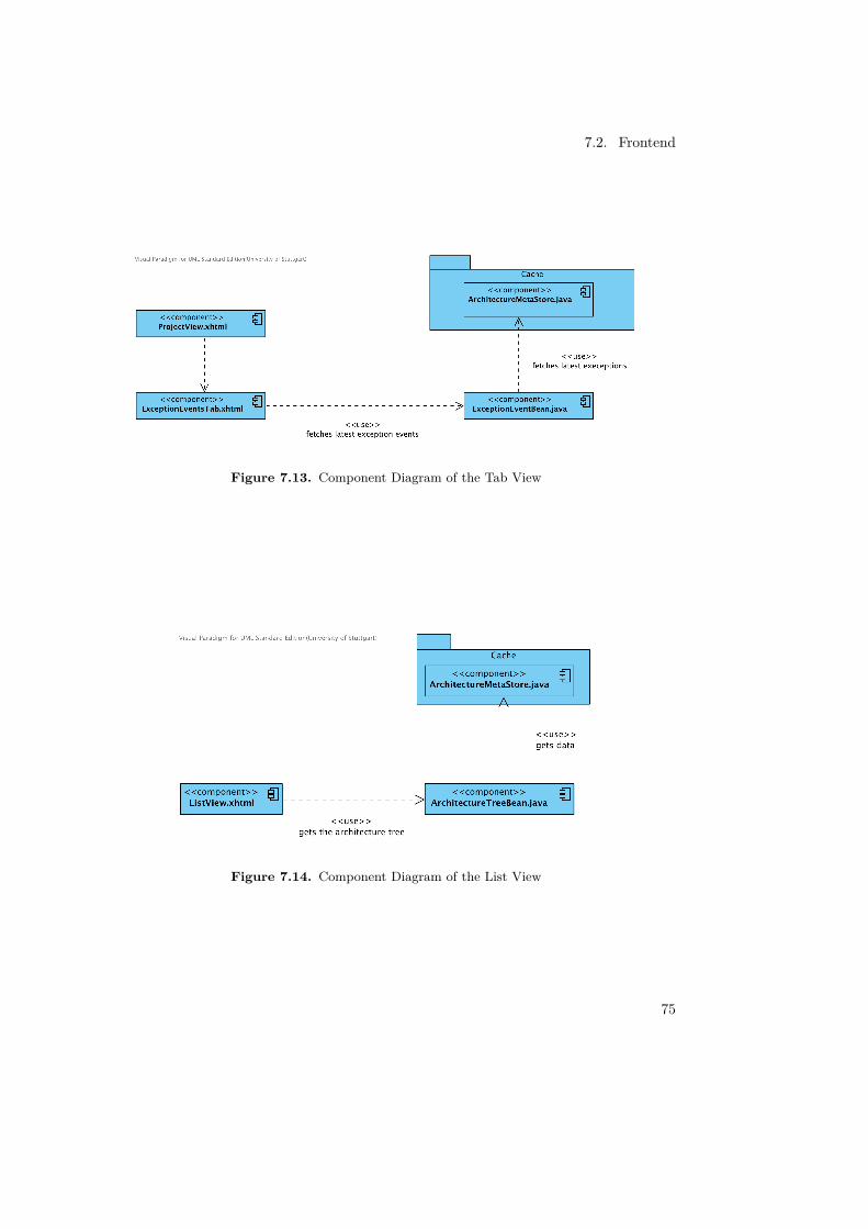
7.2. Frontend
Figure 7.13. Component Diagram of the Tab View
Figure 7.14. Component Diagram of the List View
75
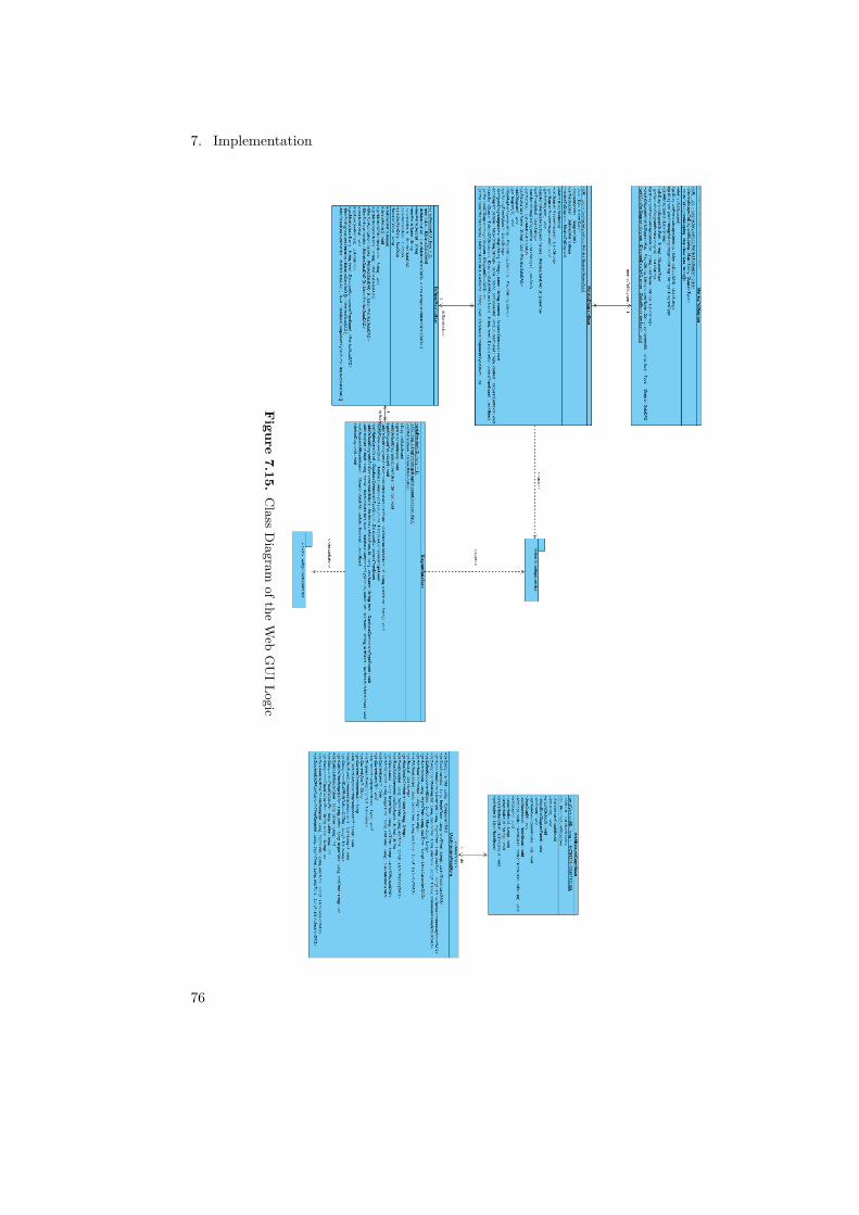
7. Implementation
Figure
7.15.C
lassD
iagramofthe
Web
GU
ILogic
76
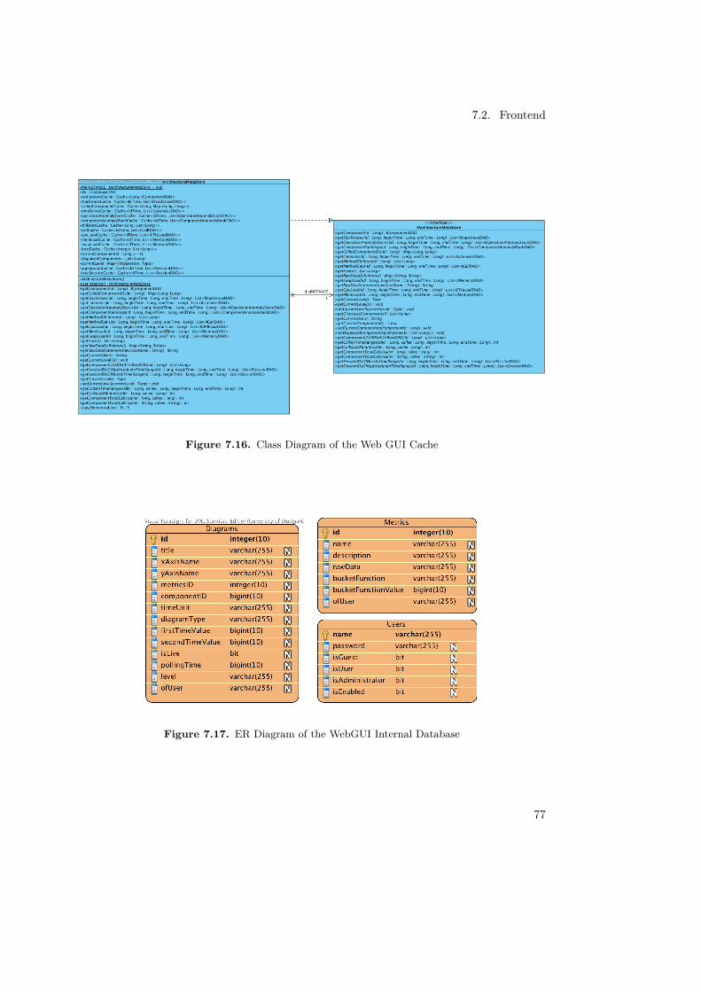
7.2. Frontend
Figure 7.16. Class Diagram of the Web GUI Cache
Figure 7.17. ER Diagram of the WebGUI Internal Database
77
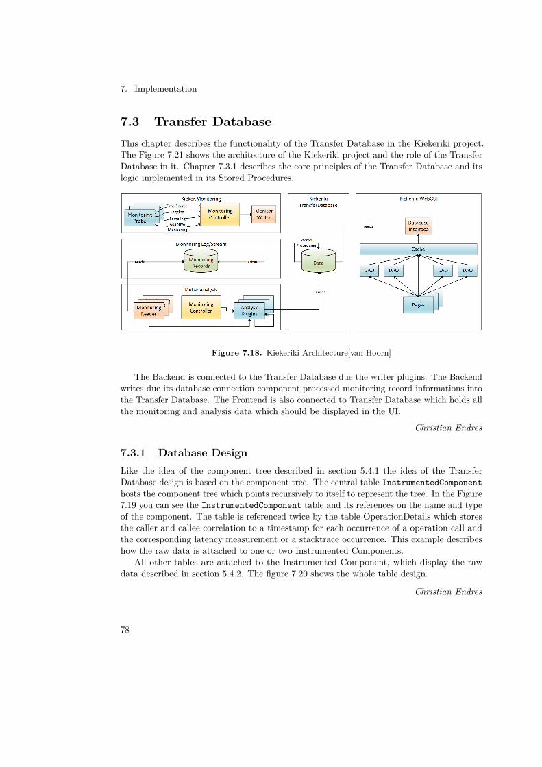
7. Implementation
7.3 Transfer DatabaseThis chapter describes the functionality of the Transfer Database in the Kiekeriki project.The Figure 7.21 shows the architecture of the Kiekeriki project and the role of the TransferDatabase in it. Chapter 7.3.1 describes the core principles of the Transfer Database and itslogic implemented in its Stored Procedures.
Figure 7.18. Kiekeriki Architecture[van Hoorn]
The Backend is connected to the Transfer Database due the writer plugins. The Backendwrites due its database connection component processed monitoring record informations intothe Transfer Database. The Frontend is also connected to Transfer Database which holds allthe monitoring and analysis data which should be displayed in the UI.
Christian Endres
7.3.1 Database DesignLike the idea of the component tree described in section 5.4.1 the idea of the TransferDatabase design is based on the component tree. The central table InstrumentedComponenthosts the component tree which points recursively to itself to represent the tree. In the Figure7.19 you can see the InstrumentedComponent table and its references on the name and typeof the component. The table is referenced twice by the table OperationDetails which storesthe caller and callee correlation to a timestamp for each occurrence of a operation call andthe corresponding latency measurement or a stacktrace occurrence. This example describeshow the raw data is attached to one or two Instrumented Components.
All other tables are attached to the Instrumented Component, which display the rawdata described in section 5.4.2. The figure 7.20 shows the whole table design.
Christian Endres
78

7.3. Transfer Database
Figure 7.19. Central table of the Transfer Database
7.3.2 Database Connections and Stored ProceduresThe MySQL-Server provides the functionality to call Stored Procedures which can encapsulateeven complex data access logic. The goal to pursue by using this functionality is to separatethe data access logic and the data processing logic. While the Kiekeriki Backend implementsthe data generation, it should not necessarily care about how to sort it into the dedicatedtables. Simple insert methods are desirable. Just as the Kiekeriki Frontend should not careabout the storage design of the data, it just wants to access the data in a convenient way.
Figure 7.21. Transfer Database data access
Database connection of the Kiekeriki Backend
The database connection of the Kiekeriki Backend cares for the write access to the TransferDatabase. Each method provided by the Interface of the database connection hides the logicof data manipulation and access to the database. There are three key concepts: First of allthe database connection knows about the stored data in the Transfer Database – especiallythe keys of already known Instrumented Components. If a new signature of a componentis inserted, the database connection cares for committing the new signature immediately.Secondly the database connection instance handles the data sets in batches, except newcomponents which are committed instantly. Thus the writing efficiency is increased because
79
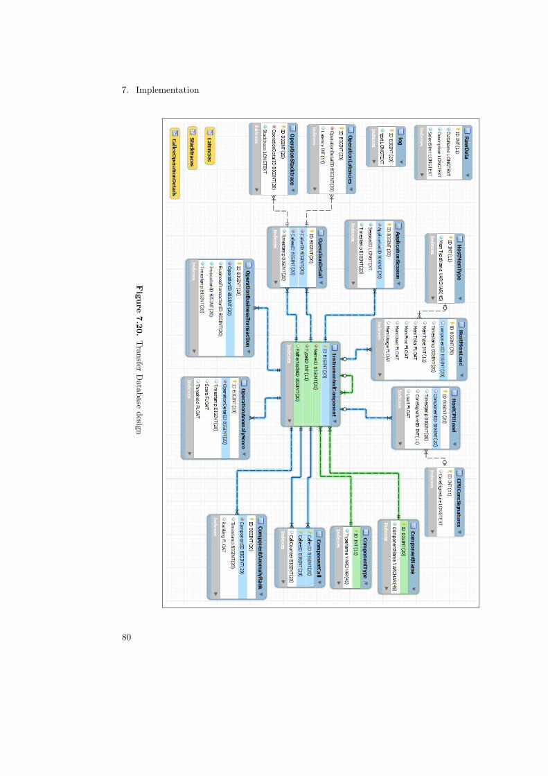
7. Implementation
Figure
7.20.Transfer
Database
design
80
7.4. Transfer Database Data Generator and Benchmarking Tool
the connection overhead per data set is reduced. Last but not least each database connectioninstance has its own thread which commits all batched data after an elapsed time. Perdefault and in respect of live monitoring the thread commits the data sets each second. Abatch is committed if it reaches a certain size or due the wait limit of the thread.
Additional aggregation of data is provided by the Stored Procedures of the MySQLServer.
Database connection of the Kiekeriki Frontend
The database connection of the Kiekeriki Frontend provides reading access to the TransferDatabase for the visualization logic. Each method provided by the Interface of the databaseconnection hides logic of data acquisition and aggregation. More complex logic like recursivelytraversing the component tree or selecting data just in a certain period of time is done byStored Procedures. The database connection component processes with the retrieved dataand returns the data processed into the internal data model.
Christian Endres
7.4 Transfer Database Data Generator and Benchmark-ing Tool
This section describes a tool which serves the Kiekeriki Frontend as generator of testdata. During the second half of the project the tool was enhanced with functionalityfor benchmarking the Transfer Database. For the sake of readability the data generationfunctionality is called Data Generator and the benchmarking functionality is called BenchmarkTool. Both are the same program, however serving to achieve different goals. The BenchmarkTool uses the same data generation, write and read functionality as the Data Generator.Though the focus of this section is on the key features and not on the programmaticallyconnections between both and the reused components. The Eclipse project is namedKiekerTransferDBDataGenerator.
The database connection components are adapted copies of the Kiekeriki Backend andFrontend. The adaptions are mostly for visibility of objects and log output to gain measure-ment data.
7.4.1 Data GeneratorThe Data Generator uses the database connection of the Kiekeriki Backend. It writesrandomly synthesised data to the Transfer Database. The synthesised data is modeled to fitthe data written by the Kiekeriki Backend. Thus RanCorr ranks are depend to the simulatedbehavior, a low latency results in a low RanCorr rank and a stacktrace occurrence results ina high RanCorr Rank which stands for anomalous behavior.
81
7. Implementation
Christian Endres
7.4.2 Benchmark ToolThe Benchmark tool uses a benchmark framework written by the IBM developer BrentBoyer [Boyer, 2008a,b,c]. The framework cares about the experiment conduction, startingwith a heating phase to the end with a summary and statistical analysis. The aim of theframework is to eliminate non deterministic measurements caused by intervention of the JavaVM like dead code analysis (DC), garbage collection and just-in-time (JIT) compiling toname some. After a heating phase there are at least 60 measurement rounds with at leastone measurement of the benchmarked functionality. If for example the compiling time differsduring the measurement rounds — the DC or JIT compiling was active — all is startedover. Eventually there is a short or a detailed statistical analysis of the benchmark. Due theresults differ with a cross test analysis done with R, the benchmark framework is used togenerate the measurement data and the analysis in chapter 8.2.3 and 8.2.4 is done with Rand RStudio.
The Benchmark Tool benchmarks the database connection of the Kiekeriki Frontendwhich retrieves data and processes it into the internal model. The benchmark of the KiekerikiBackend writes data into the Transfer Database. The conduction and the results are analysedin the chapter 8.2.
Christian Endres
82

Chapter 8
Experiments and Validation
8.1 Experiments and validation of the Kiekeriki Back-end
8.1.1 Evaluation goalsDescribed here are the goals by which the Kiekeriki backend should be evaluated.
83
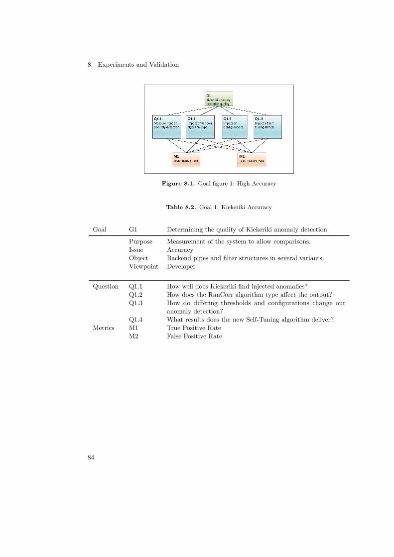
8. Experiments and Validation
Figure 8.1. Goal figure 1: High Accuracy
Table 8.2. Goal 1: Kiekeriki Accuracy
Goal G1 Determining the quality of Kiekeriki anomaly detection.
Purpose Measurement of the system to allow comparisons.Issue AccuracyObject Backend pipes and filter structures in several variants.Viewpoint Developer
Question Q1.1 How well does Kiekeriki find injected anomalies?Q1.2 How does the RanCorr algorithm type affect the output?Q1.3 How do differing thresholds and configurations change our
anomaly detection?Q1.4 What results does the new Self-Tuning algorithm deliver?
Metrics M1 True Positive RateM2 False Positive Rate
84
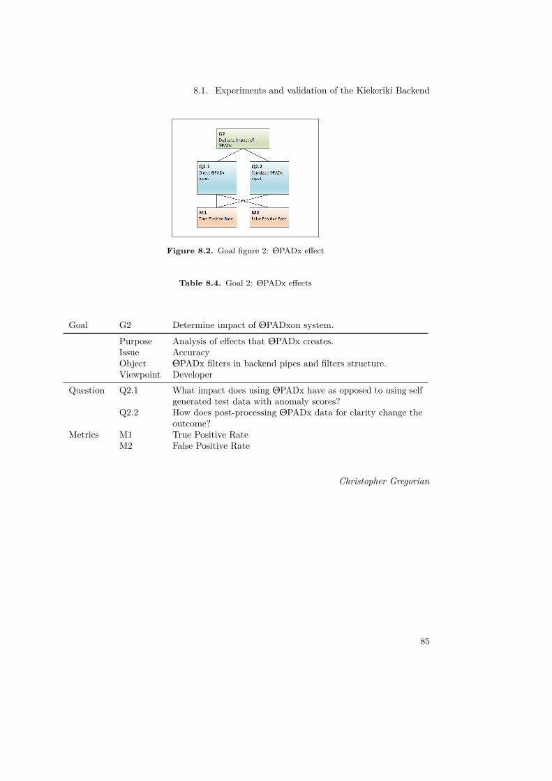
8.1. Experiments and validation of the Kiekeriki Backend
Figure 8.2. Goal figure 2: ΘPADx effect
Table 8.4. Goal 2: ΘPADx effects
Goal G2 Determine impact of ΘPADxon system.
Purpose Analysis of effects that ΘPADx creates.Issue AccuracyObject ΘPADx filters in backend pipes and filters structure.Viewpoint Developer
Question Q2.1 What impact does using ΘPADx have as opposed to using selfgenerated test data with anomaly scores?
Q2.2 How does post-processing ΘPADx data for clarity change theoutcome?
Metrics M1 True Positive RateM2 False Positive Rate
Christopher Gregorian
85

8. Experiments and Validation
8.1.2 Experimental designThis section describes the experiments that allows finding answers to the questions noted inSection 8.1.1. To allow the generation and gathering of data, the Kieker pipes and filtersarchitecture was extended with several filters to surround the ΘPADx and RanCorr filters.
Pipes and Filters setup
As can be seen in Figure 8.3,both the ΘPADx and RanCorr filters are surrounded by thetest framework filters to allow controlling data in and outputs.
Figure 8.3. Experiment setup
The following list describes the additionally developed evaluation tools:• Data Generator - A filter that creates data according to a static hierarchy. Will inject
anomalies into the data for the system to find. See Section 8.1.2.• RanCorr Offline Evaluator - designed to use the anomaly data from the Data Generator
as well as the RanCorr output data. Will iterate evaluating the data with an internalthreshold starting at 0.05 and incrementing by 0.05 until 1.00 and return the resultsfor each evaluation.
• Data Aggregator - Takes the data from several runs and aggregates them into onedataset for ease of use. See Section 8.1.2 for details.
Paths through Pipes-and-Filters
On Display in Figure 8.3 are three different paths that the data takes through our pipesand filters structure. Constant connections that always exist are marked in black. These
86
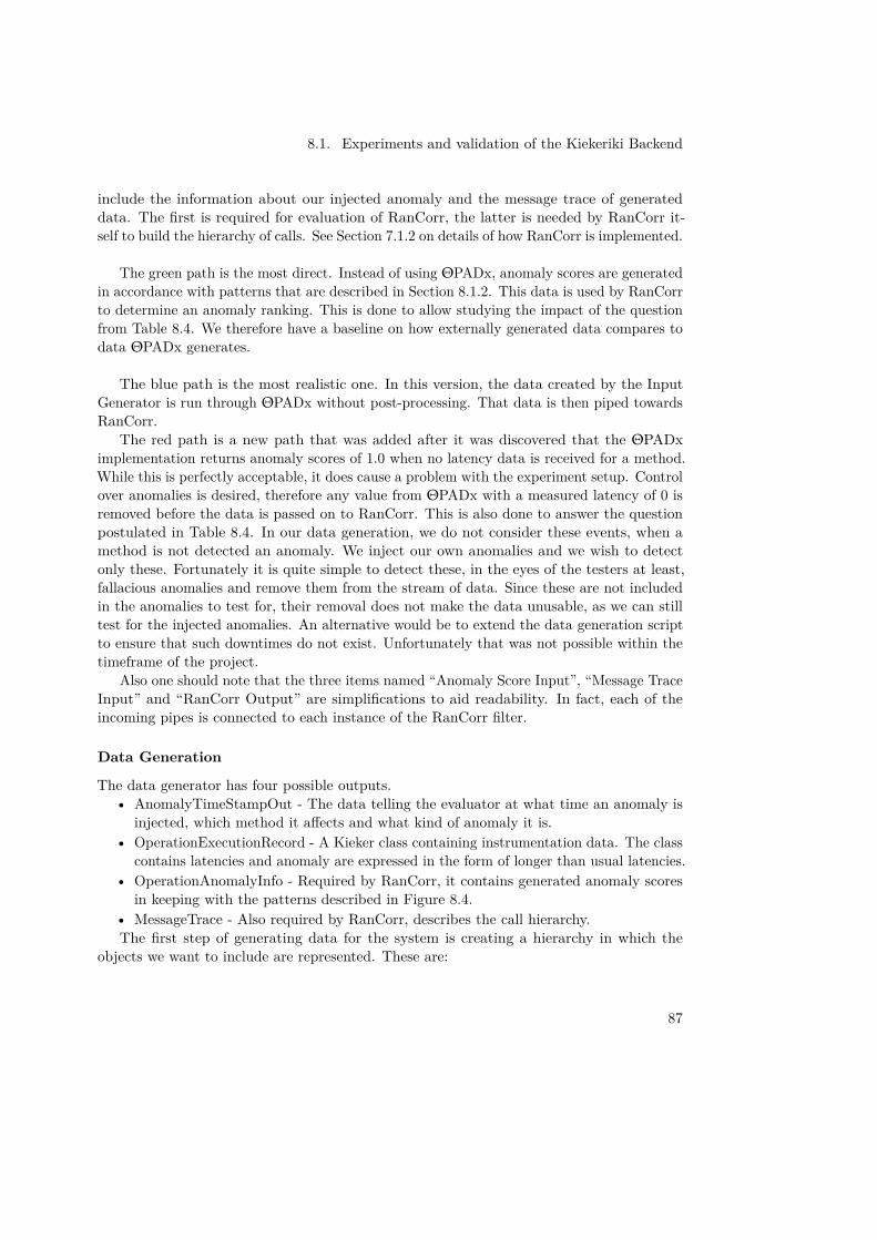
8.1. Experiments and validation of the Kiekeriki Backend
include the information about our injected anomaly and the message trace of generateddata. The first is required for evaluation of RanCorr, the latter is needed by RanCorr it-self to build the hierarchy of calls. See Section 7.1.2 on details of how RanCorr is implemented.
The green path is the most direct. Instead of using ΘPADx, anomaly scores are generatedin accordance with patterns that are described in Section 8.1.2. This data is used by RanCorrto determine an anomaly ranking. This is done to allow studying the impact of the questionfrom Table 8.4. We therefore have a baseline on how externally generated data compares todata ΘPADx generates.
The blue path is the most realistic one. In this version, the data created by the InputGenerator is run through ΘPADx without post-processing. That data is then piped towardsRanCorr.
The red path is a new path that was added after it was discovered that the ΘPADximplementation returns anomaly scores of 1.0 when no latency data is received for a method.While this is perfectly acceptable, it does cause a problem with the experiment setup. Controlover anomalies is desired, therefore any value from ΘPADx with a measured latency of 0 isremoved before the data is passed on to RanCorr. This is also done to answer the questionpostulated in Table 8.4. In our data generation, we do not consider these events, when amethod is not detected an anomaly. We inject our own anomalies and we wish to detectonly these. Fortunately it is quite simple to detect these, in the eyes of the testers at least,fallacious anomalies and remove them from the stream of data. Since these are not includedin the anomalies to test for, their removal does not make the data unusable, as we can stilltest for the injected anomalies. An alternative would be to extend the data generation scriptto ensure that such downtimes do not exist. Unfortunately that was not possible within thetimeframe of the project.
Also one should note that the three items named “Anomaly Score Input”, “Message TraceInput” and “RanCorr Output” are simplifications to aid readability. In fact, each of theincoming pipes is connected to each instance of the RanCorr filter.
Data Generation
The data generator has four possible outputs.• AnomalyTimeStampOut - The data telling the evaluator at what time an anomaly is
injected, which method it affects and what kind of anomaly it is.• OperationExecutionRecord - A Kieker class containing instrumentation data. The class
contains latencies and anomaly are expressed in the form of longer than usual latencies.• OperationAnomalyInfo - Required by RanCorr, it contains generated anomaly scores
in keeping with the patterns described in Figure 8.4.• MessageTrace - Also required by RanCorr, describes the call hierarchy.The first step of generating data for the system is creating a hierarchy in which the
objects we want to include are represented. These are:
87
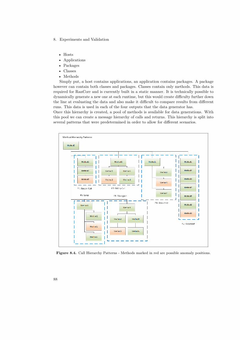
8. Experiments and Validation
• Hosts• Applications• Packages• Classes• MethodsSimply put, a host contains applications, an application contains packages. A package
however can contain both classes and packages. Classes contain only methods. This data isrequired for RanCorr and is currently built in a static manner. It is technically possible todynamically generate a new one at each runtime, but this would create difficulty further downthe line at evaluating the data and also make it difficult to compare results from differentruns. This data is used in each of the four outputs that the data generator has.Once this hierarchy is created, a pool of methods is available for data generations. Withthis pool we can create a message hierarchy of calls and returns. This hierarchy is split intoseveral patterns that were predetermined in order to allow for different scenarios.
Figure 8.4. Call Hierarchy Patterns - Methods marked in red are possible anomaly positions.
88
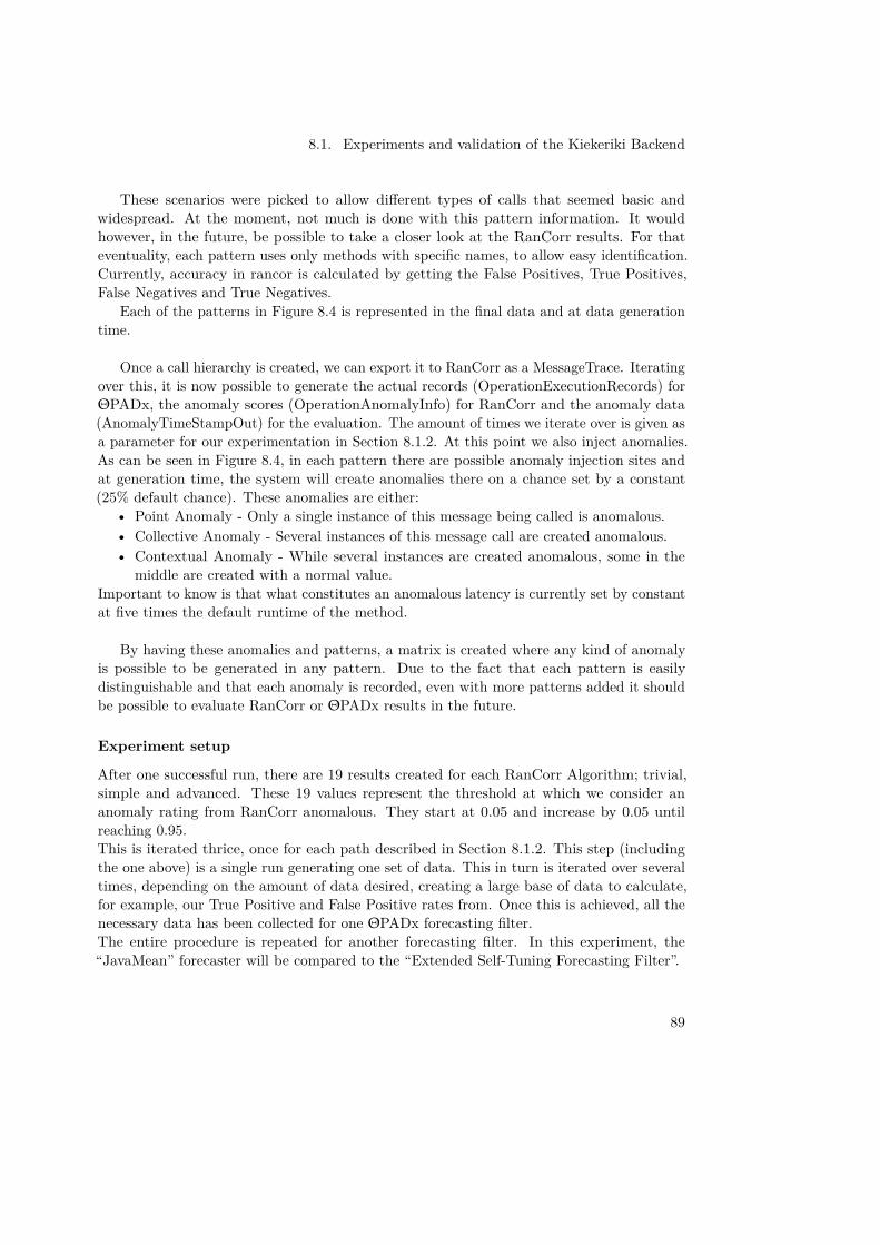
8.1. Experiments and validation of the Kiekeriki Backend
These scenarios were picked to allow different types of calls that seemed basic andwidespread. At the moment, not much is done with this pattern information. It wouldhowever, in the future, be possible to take a closer look at the RanCorr results. For thateventuality, each pattern uses only methods with specific names, to allow easy identification.Currently, accuracy in rancor is calculated by getting the False Positives, True Positives,False Negatives and True Negatives.
Each of the patterns in Figure 8.4 is represented in the final data and at data generationtime.
Once a call hierarchy is created, we can export it to RanCorr as a MessageTrace. Iteratingover this, it is now possible to generate the actual records (OperationExecutionRecords) forΘPADx, the anomaly scores (OperationAnomalyInfo) for RanCorr and the anomaly data(AnomalyTimeStampOut) for the evaluation. The amount of times we iterate over is given asa parameter for our experimentation in Section 8.1.2. At this point we also inject anomalies.As can be seen in Figure 8.4, in each pattern there are possible anomaly injection sites andat generation time, the system will create anomalies there on a chance set by a constant(25% default chance). These anomalies are either:
• Point Anomaly - Only a single instance of this message being called is anomalous.• Collective Anomaly - Several instances of this message call are created anomalous.• Contextual Anomaly - While several instances are created anomalous, some in the
middle are created with a normal value.Important to know is that what constitutes an anomalous latency is currently set by constantat five times the default runtime of the method.
By having these anomalies and patterns, a matrix is created where any kind of anomalyis possible to be generated in any pattern. Due to the fact that each pattern is easilydistinguishable and that each anomaly is recorded, even with more patterns added it shouldbe possible to evaluate RanCorr or ΘPADx results in the future.
Experiment setup
After one successful run, there are 19 results created for each RanCorr Algorithm; trivial,simple and advanced. These 19 values represent the threshold at which we consider ananomaly rating from RanCorr anomalous. They start at 0.05 and increase by 0.05 untilreaching 0.95.This is iterated thrice, once for each path described in Section 8.1.2. This step (includingthe one above) is a single run generating one set of data. This in turn is iterated over severaltimes, depending on the amount of data desired, creating a large base of data to calculate,for example, our True Positive and False Positive rates from. Once this is achieved, all thenecessary data has been collected for one ΘPADx forecasting filter.The entire procedure is repeated for another forecasting filter. In this experiment, the“JavaMean” forecaster will be compared to the “Extended Self-Tuning Forecasting Filter”.
89
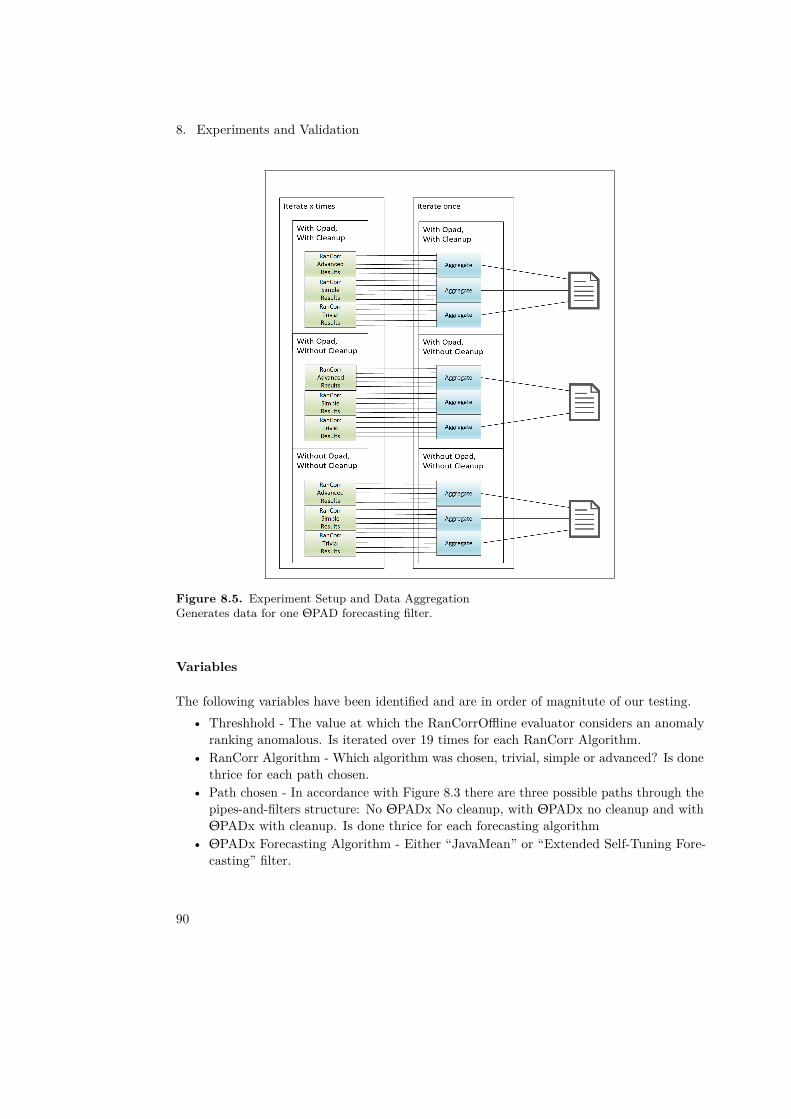
8. Experiments and Validation
Figure 8.5. Experiment Setup and Data AggregationGenerates data for one ΘPAD forecasting filter.
Variables
The following variables have been identified and are in order of magnitute of our testing.• Threshhold - The value at which the RanCorrOffline evaluator considers an anomaly
ranking anomalous. Is iterated over 19 times for each RanCorr Algorithm.• RanCorr Algorithm - Which algorithm was chosen, trivial, simple or advanced? Is done
thrice for each path chosen.• Path chosen - In accordance with Figure 8.3 there are three possible paths through the
pipes-and-filters structure: No ΘPADx No cleanup, with ΘPADx no cleanup and withΘPADx with cleanup. Is done thrice for each forecasting algorithm
• ΘPADx Forecasting Algorithm - Either “JavaMean” or “Extended Self-Tuning Fore-casting” filter.
90
8.1. Experiments and validation of the Kiekeriki Backend
Data Aggregation
The data aggregation takes data generated by a large amount of runs and condenses itinto one set. This is accomplished by gathering the True Positives, True Negatives, FalsePositives and False Negatives of all corresponding data into one new set. Each time theaverage RanCorrAccuracy and RanCorrClearness are calculated and stored. At the veryend, the Accuracy, Precision, F-Measure, True Positive Rate and False Positive Rate arecalculated for the corresponding data set.In this case, corresponding data refers to data sets that are run with the same setup (forexample; With Opad, Without Cleanup), are measured using the same RanCorr algorithm(Trivial, Simple, Advanced) and are also calculated with an identical threshold.
Experiment execution
The execution of the experiment contains two phases as mentioned in Section 8.1.2, one foreach ΘPAD forecasting filter. For each of these, a script is run which handles the iterationsdescribed. The default value for iterations for one forecasting filter is 100. Once all ofthese have been run the data aggregator is started, condensing our results to a three setof 19 results for each of the three RanCorr algorithms, one set for each path described inSection 8.1.2. This data is ready for analysis and will create an overview of the quality ofRanCorr with a specific forecasting filter.
Christopher Gregorian
8.1.3 Experiment data and resultsJavaMean Results
First, the aggregated results created using the “JavaMean” forecasting filter.
91
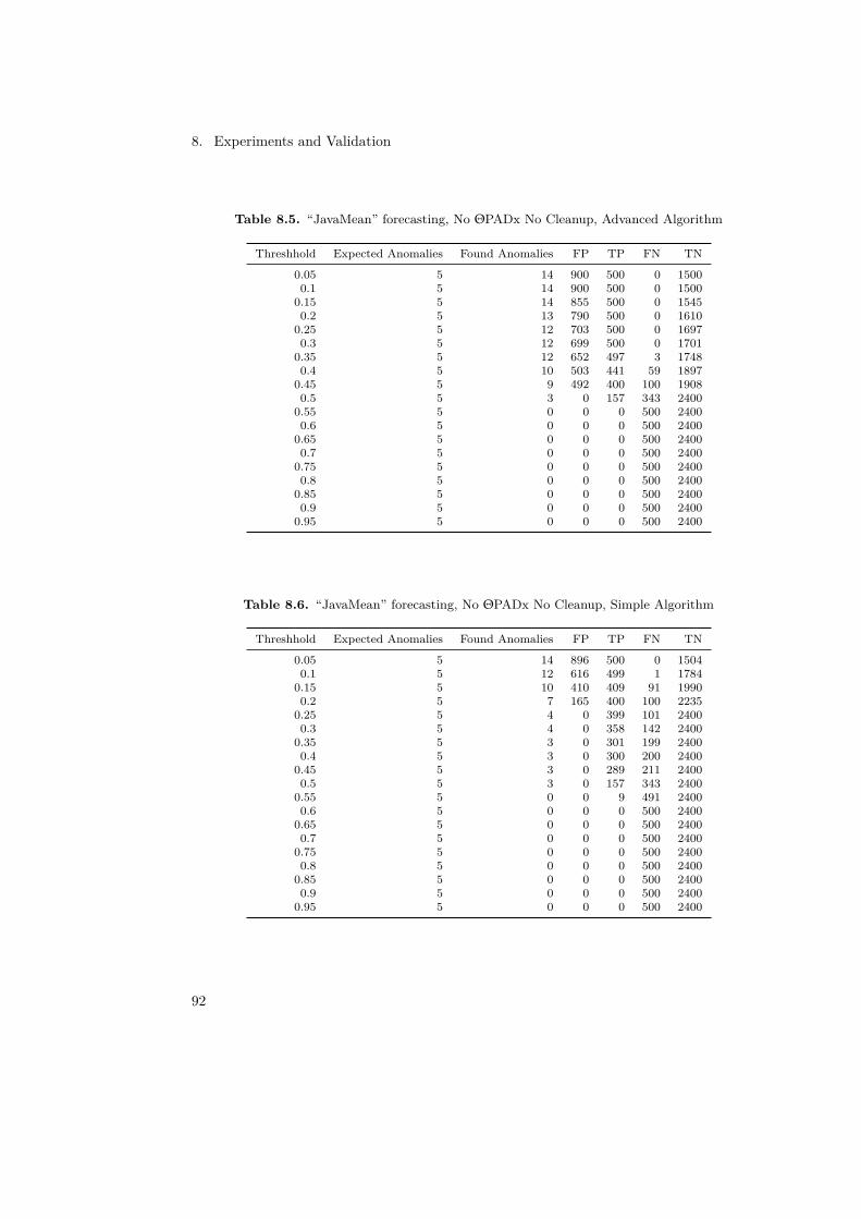
8. Experiments and Validation
Table 8.5. “JavaMean” forecasting, No ΘPADx No Cleanup, Advanced Algorithm
Threshhold Expected Anomalies Found Anomalies FP TP FN TN
0.05 5 14 900 500 0 15000.1 5 14 900 500 0 1500
0.15 5 14 855 500 0 15450.2 5 13 790 500 0 1610
0.25 5 12 703 500 0 16970.3 5 12 699 500 0 1701
0.35 5 12 652 497 3 17480.4 5 10 503 441 59 1897
0.45 5 9 492 400 100 19080.5 5 3 0 157 343 2400
0.55 5 0 0 0 500 24000.6 5 0 0 0 500 2400
0.65 5 0 0 0 500 24000.7 5 0 0 0 500 2400
0.75 5 0 0 0 500 24000.8 5 0 0 0 500 2400
0.85 5 0 0 0 500 24000.9 5 0 0 0 500 2400
0.95 5 0 0 0 500 2400
Table 8.6. “JavaMean” forecasting, No ΘPADx No Cleanup, Simple Algorithm
Threshhold Expected Anomalies Found Anomalies FP TP FN TN
0.05 5 14 896 500 0 15040.1 5 12 616 499 1 1784
0.15 5 10 410 409 91 19900.2 5 7 165 400 100 2235
0.25 5 4 0 399 101 24000.3 5 4 0 358 142 2400
0.35 5 3 0 301 199 24000.4 5 3 0 300 200 2400
0.45 5 3 0 289 211 24000.5 5 3 0 157 343 2400
0.55 5 0 0 9 491 24000.6 5 0 0 0 500 2400
0.65 5 0 0 0 500 24000.7 5 0 0 0 500 2400
0.75 5 0 0 0 500 24000.8 5 0 0 0 500 2400
0.85 5 0 0 0 500 24000.9 5 0 0 0 500 2400
0.95 5 0 0 0 500 2400
92
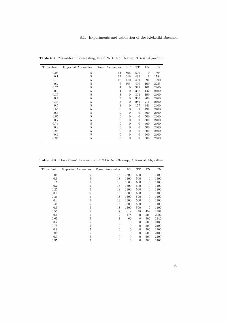
8.1. Experiments and validation of the Kiekeriki Backend
Table 8.7. “JavaMean” forecasting, No ΘPADx No Cleanup, Trivial Algorithm
Threshhold Expected Anomalies Found Anomalies FP TP FN TN
0.05 5 14 896 500 0 15040.1 5 12 616 499 1 1784
0.15 5 10 410 409 91 19900.2 5 7 165 400 100 2235
0.25 5 4 0 399 101 24000.3 5 4 0 358 142 2400
0.35 5 3 0 301 199 24000.4 5 3 0 300 200 2400
0.45 5 3 0 289 211 24000.5 5 3 0 157 343 2400
0.55 5 0 0 9 491 24000.6 5 0 0 0 500 2400
0.65 5 0 0 0 500 24000.7 5 0 0 0 500 2400
0.75 5 0 0 0 500 24000.8 5 0 0 0 500 2400
0.85 5 0 0 0 500 24000.9 5 0 0 0 500 2400
0.95 5 0 0 0 500 2400
Table 8.8. “JavaMean” forecasting, ΘPADx No Cleanup, Advanced Algorithm
Threshhold Expected Anomalies Found Anomalies FP TP FN TN
0.05 5 18 1300 500 0 11000.1 5 18 1300 500 0 1100
0.15 5 18 1300 500 0 11000.2 5 18 1300 500 0 1100
0.25 5 18 1300 500 0 11000.3 5 18 1300 500 0 1100
0.35 5 18 1300 500 0 11000.4 5 18 1300 500 0 1100
0.45 5 18 1300 500 0 11000.5 5 18 1300 500 0 1100
0.55 5 7 619 48 452 17810.6 5 2 178 0 500 2222
0.65 5 1 60 0 500 23400.7 5 0 0 0 500 2400
0.75 5 0 0 0 500 24000.8 5 0 0 0 500 2400
0.85 5 0 0 0 500 24000.9 5 0 0 0 500 2400
0.95 5 0 0 0 500 2400
93
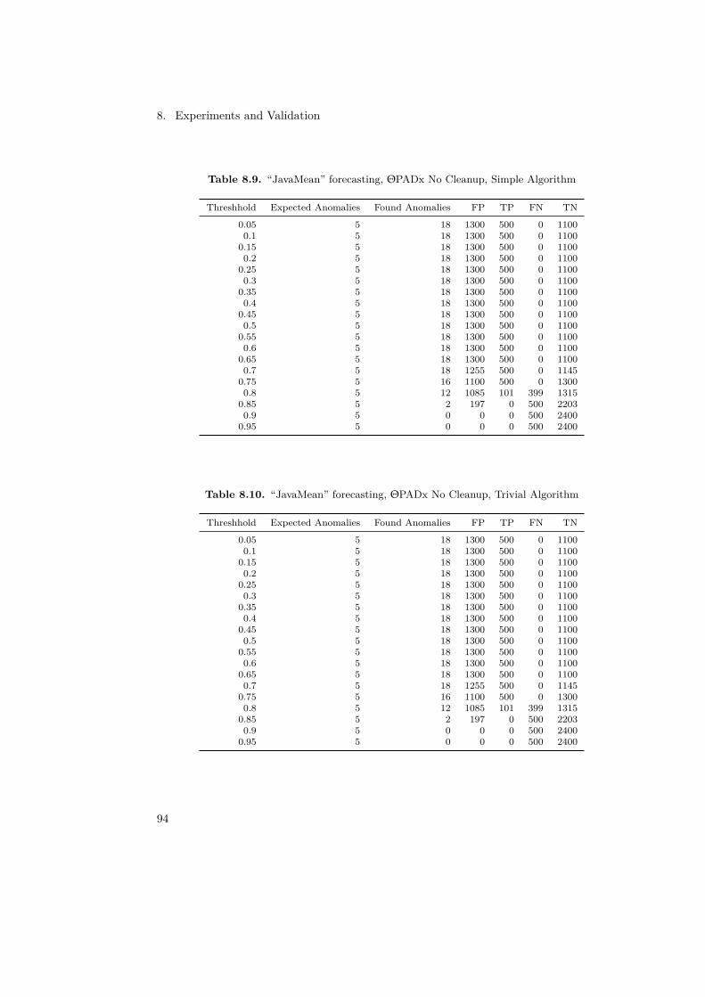
8. Experiments and Validation
Table 8.9. “JavaMean” forecasting, ΘPADx No Cleanup, Simple Algorithm
Threshhold Expected Anomalies Found Anomalies FP TP FN TN
0.05 5 18 1300 500 0 11000.1 5 18 1300 500 0 1100
0.15 5 18 1300 500 0 11000.2 5 18 1300 500 0 1100
0.25 5 18 1300 500 0 11000.3 5 18 1300 500 0 1100
0.35 5 18 1300 500 0 11000.4 5 18 1300 500 0 1100
0.45 5 18 1300 500 0 11000.5 5 18 1300 500 0 1100
0.55 5 18 1300 500 0 11000.6 5 18 1300 500 0 1100
0.65 5 18 1300 500 0 11000.7 5 18 1255 500 0 1145
0.75 5 16 1100 500 0 13000.8 5 12 1085 101 399 1315
0.85 5 2 197 0 500 22030.9 5 0 0 0 500 2400
0.95 5 0 0 0 500 2400
Table 8.10. “JavaMean” forecasting, ΘPADx No Cleanup, Trivial Algorithm
Threshhold Expected Anomalies Found Anomalies FP TP FN TN
0.05 5 18 1300 500 0 11000.1 5 18 1300 500 0 1100
0.15 5 18 1300 500 0 11000.2 5 18 1300 500 0 1100
0.25 5 18 1300 500 0 11000.3 5 18 1300 500 0 1100
0.35 5 18 1300 500 0 11000.4 5 18 1300 500 0 1100
0.45 5 18 1300 500 0 11000.5 5 18 1300 500 0 1100
0.55 5 18 1300 500 0 11000.6 5 18 1300 500 0 1100
0.65 5 18 1300 500 0 11000.7 5 18 1255 500 0 1145
0.75 5 16 1100 500 0 13000.8 5 12 1085 101 399 1315
0.85 5 2 197 0 500 22030.9 5 0 0 0 500 2400
0.95 5 0 0 0 500 2400
94

8.1. Experiments and validation of the Kiekeriki Backend
Table 8.11. “JavaMean” forecasting, ΘPADx Cleanup, Advanced Algorithm
Threshhold Expected Anomalies Found Anomalies FP TP FN TN
0.05 5 12 893 500 0 15070.1 5 11 736 441 59 1664
0.15 5 11 712 415 85 16880.2 5 11 700 400 100 1700
0.25 5 11 700 400 100 17000.3 5 11 700 400 100 1700
0.35 5 11 700 400 100 17000.4 5 11 700 400 100 1700
0.45 5 11 700 400 100 17000.5 5 2 151 87 413 2249
0.55 5 0 0 0 500 24000.6 5 0 0 0 500 2400
0.65 5 0 0 0 500 24000.7 5 0 0 0 500 2400
0.75 5 0 0 0 500 24000.8 5 0 0 0 500 2400
0.85 5 0 0 0 500 24000.9 5 0 0 0 500 2400
0.95 5 0 0 0 500 2400
Table 8.12. “JavaMean” forecasting, ΘPADx Cleanup, Simple Algorithm
Threshhold Expected Anomalies Found Anomalies FP TP FN TN
0.05 5 12 709 498 2 16910.1 5 11 700 400 100 1700
0.15 5 11 700 400 100 17000.2 5 11 700 400 100 1700
0.25 5 11 700 400 100 17000.3 5 11 700 400 100 1700
0.35 5 11 700 386 114 17000.4 5 8 635 111 389 1765
0.45 5 3 192 96 404 22080.5 5 1 121 39 461 2279
0.55 5 1 18 0 500 23820.6 5 0 0 0 500 2400
0.65 5 0 0 0 500 24000.7 5 0 0 0 500 2400
0.75 5 0 0 0 500 24000.8 5 0 0 0 500 2400
0.85 5 0 0 0 500 24000.9 5 0 0 0 500 2400
0.95 5 0 0 0 500 2400
95
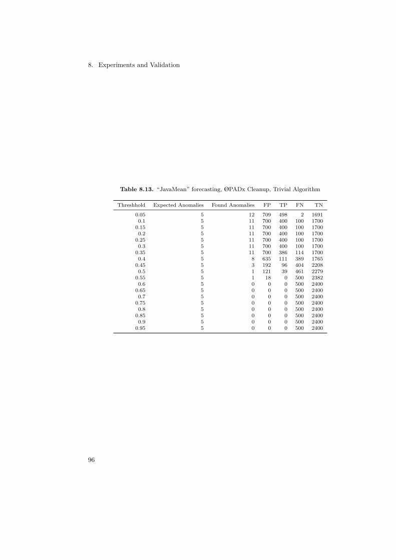
8. Experiments and Validation
Table 8.13. “JavaMean” forecasting, ΘPADx Cleanup, Trivial Algorithm
Threshhold Expected Anomalies Found Anomalies FP TP FN TN
0.05 5 12 709 498 2 16910.1 5 11 700 400 100 1700
0.15 5 11 700 400 100 17000.2 5 11 700 400 100 1700
0.25 5 11 700 400 100 17000.3 5 11 700 400 100 1700
0.35 5 11 700 386 114 17000.4 5 8 635 111 389 1765
0.45 5 3 192 96 404 22080.5 5 1 121 39 461 2279
0.55 5 1 18 0 500 23820.6 5 0 0 0 500 2400
0.65 5 0 0 0 500 24000.7 5 0 0 0 500 2400
0.75 5 0 0 0 500 24000.8 5 0 0 0 500 2400
0.85 5 0 0 0 500 24000.9 5 0 0 0 500 2400
0.95 5 0 0 0 500 2400
96

8.1. Experiments and validation of the Kiekeriki Backend
Extended Self-Tuning Forecast Results
The data measured using the Self-Tuning Forecast.
Table 8.14. “Extended Self-Tuning” forecasting, No ΘPADx No Cleanup, Advanced Algorithm
Threshhold Expected Anomalies Found Anomalies FP TP FN TN
0.05 5 14 900 500 0 15000.1 5 14 900 500 0 1500
0.15 5 14 843 500 0 15570.2 5 13 784 500 0 1616
0.25 5 12 702 500 0 16980.3 5 12 700 500 0 1700
0.35 5 12 633 495 5 17670.4 5 10 503 428 72 1897
0.45 5 9 492 400 100 19080.5 5 3 0 136 364 2400
0.55 5 0 0 0 500 24000.6 5 0 0 0 500 2400
0.65 5 0 0 0 500 24000.7 5 0 0 0 500 2400
0.75 5 0 0 0 500 24000.8 5 0 0 0 500 2400
0.85 5 0 0 0 500 24000.9 5 0 0 0 500 2400
0.95 5 0 0 0 500 2400
Table 8.15. “Extended Self-Tuning” forecasting, No ΘPADx No Cleanup, Simple Algorithm
Threshhold Expected Anomalies Found Anomalies FP TP FN TN
0.05 5 14 899 500 0 15010.1 5 12 592 498 2 1808
0.15 5 9 386 407 93 20140.2 5 7 135 400 100 2265
0.25 5 4 0 399 101 24000.3 5 4 0 352 148 2400
0.35 5 3 0 303 197 24000.4 5 3 0 300 200 2400
0.45 5 3 0 282 218 24000.5 5 3 0 136 364 2400
0.55 5 0 0 4 496 24000.6 5 0 0 0 500 2400
0.65 5 0 0 0 500 24000.7 5 0 0 0 500 2400
0.75 5 0 0 0 500 24000.8 5 0 0 0 500 2400
0.85 5 0 0 0 500 24000.9 5 0 0 0 500 2400
0.95 5 0 0 0 500 2400
97
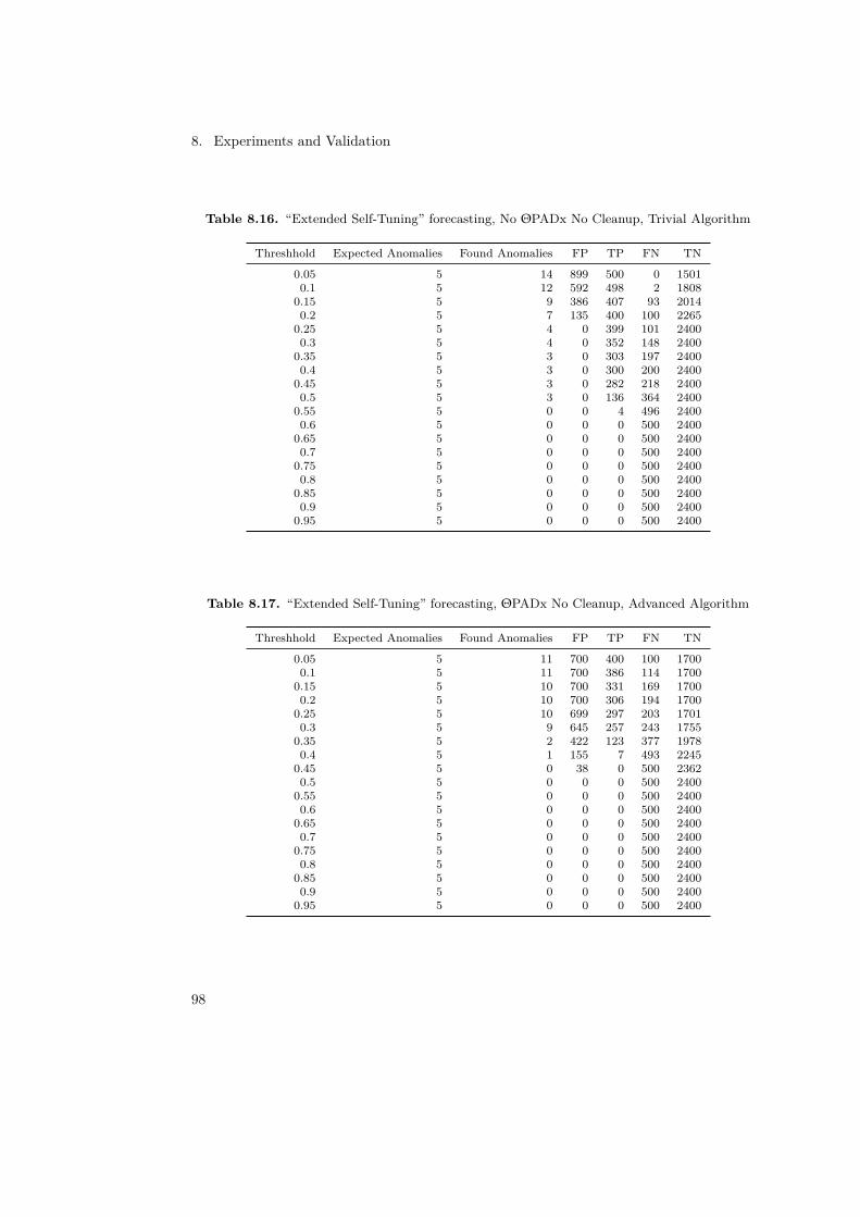
8. Experiments and Validation
Table 8.16. “Extended Self-Tuning” forecasting, No ΘPADx No Cleanup, Trivial Algorithm
Threshhold Expected Anomalies Found Anomalies FP TP FN TN
0.05 5 14 899 500 0 15010.1 5 12 592 498 2 1808
0.15 5 9 386 407 93 20140.2 5 7 135 400 100 2265
0.25 5 4 0 399 101 24000.3 5 4 0 352 148 2400
0.35 5 3 0 303 197 24000.4 5 3 0 300 200 2400
0.45 5 3 0 282 218 24000.5 5 3 0 136 364 2400
0.55 5 0 0 4 496 24000.6 5 0 0 0 500 2400
0.65 5 0 0 0 500 24000.7 5 0 0 0 500 2400
0.75 5 0 0 0 500 24000.8 5 0 0 0 500 2400
0.85 5 0 0 0 500 24000.9 5 0 0 0 500 2400
0.95 5 0 0 0 500 2400
Table 8.17. “Extended Self-Tuning” forecasting, ΘPADx No Cleanup, Advanced Algorithm
Threshhold Expected Anomalies Found Anomalies FP TP FN TN
0.05 5 11 700 400 100 17000.1 5 11 700 386 114 1700
0.15 5 10 700 331 169 17000.2 5 10 700 306 194 1700
0.25 5 10 699 297 203 17010.3 5 9 645 257 243 1755
0.35 5 2 422 123 377 19780.4 5 1 155 7 493 2245
0.45 5 0 38 0 500 23620.5 5 0 0 0 500 2400
0.55 5 0 0 0 500 24000.6 5 0 0 0 500 2400
0.65 5 0 0 0 500 24000.7 5 0 0 0 500 2400
0.75 5 0 0 0 500 24000.8 5 0 0 0 500 2400
0.85 5 0 0 0 500 24000.9 5 0 0 0 500 2400
0.95 5 0 0 0 500 2400
98
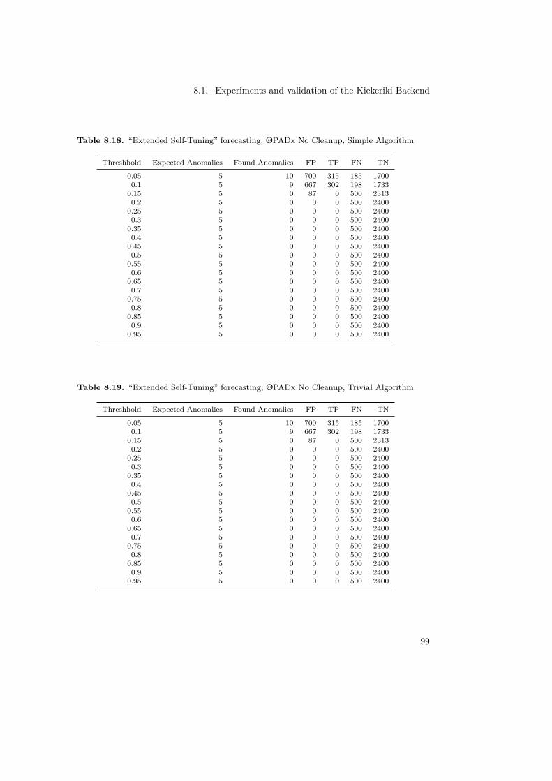
8.1. Experiments and validation of the Kiekeriki Backend
Table 8.18. “Extended Self-Tuning” forecasting, ΘPADx No Cleanup, Simple Algorithm
Threshhold Expected Anomalies Found Anomalies FP TP FN TN
0.05 5 10 700 315 185 17000.1 5 9 667 302 198 1733
0.15 5 0 87 0 500 23130.2 5 0 0 0 500 2400
0.25 5 0 0 0 500 24000.3 5 0 0 0 500 2400
0.35 5 0 0 0 500 24000.4 5 0 0 0 500 2400
0.45 5 0 0 0 500 24000.5 5 0 0 0 500 2400
0.55 5 0 0 0 500 24000.6 5 0 0 0 500 2400
0.65 5 0 0 0 500 24000.7 5 0 0 0 500 2400
0.75 5 0 0 0 500 24000.8 5 0 0 0 500 2400
0.85 5 0 0 0 500 24000.9 5 0 0 0 500 2400
0.95 5 0 0 0 500 2400
Table 8.19. “Extended Self-Tuning” forecasting, ΘPADx No Cleanup, Trivial Algorithm
Threshhold Expected Anomalies Found Anomalies FP TP FN TN
0.05 5 10 700 315 185 17000.1 5 9 667 302 198 1733
0.15 5 0 87 0 500 23130.2 5 0 0 0 500 2400
0.25 5 0 0 0 500 24000.3 5 0 0 0 500 2400
0.35 5 0 0 0 500 24000.4 5 0 0 0 500 2400
0.45 5 0 0 0 500 24000.5 5 0 0 0 500 2400
0.55 5 0 0 0 500 24000.6 5 0 0 0 500 2400
0.65 5 0 0 0 500 24000.7 5 0 0 0 500 2400
0.75 5 0 0 0 500 24000.8 5 0 0 0 500 2400
0.85 5 0 0 0 500 24000.9 5 0 0 0 500 2400
0.95 5 0 0 0 500 2400
99
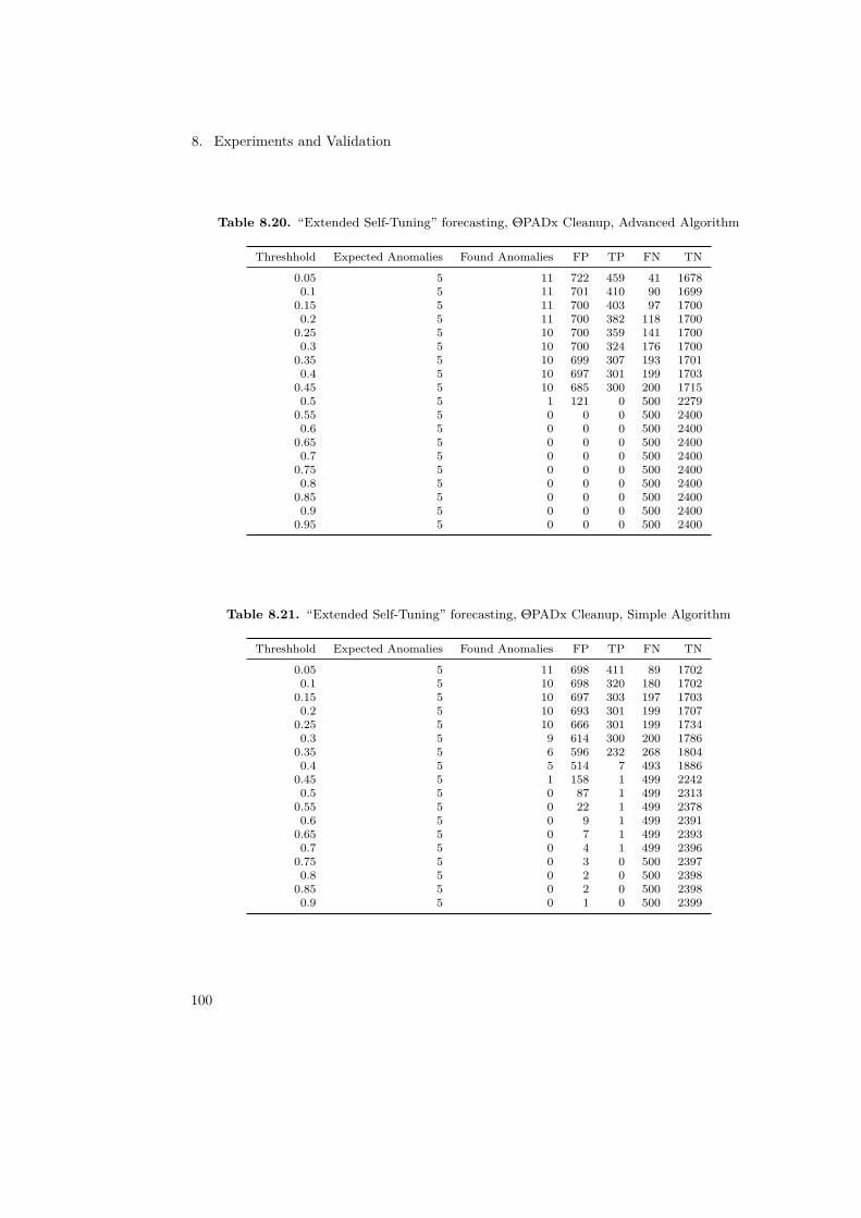
8. Experiments and Validation
Table 8.20. “Extended Self-Tuning” forecasting, ΘPADx Cleanup, Advanced Algorithm
Threshhold Expected Anomalies Found Anomalies FP TP FN TN
0.05 5 11 722 459 41 16780.1 5 11 701 410 90 1699
0.15 5 11 700 403 97 17000.2 5 11 700 382 118 1700
0.25 5 10 700 359 141 17000.3 5 10 700 324 176 1700
0.35 5 10 699 307 193 17010.4 5 10 697 301 199 1703
0.45 5 10 685 300 200 17150.5 5 1 121 0 500 2279
0.55 5 0 0 0 500 24000.6 5 0 0 0 500 2400
0.65 5 0 0 0 500 24000.7 5 0 0 0 500 2400
0.75 5 0 0 0 500 24000.8 5 0 0 0 500 2400
0.85 5 0 0 0 500 24000.9 5 0 0 0 500 2400
0.95 5 0 0 0 500 2400
Table 8.21. “Extended Self-Tuning” forecasting, ΘPADx Cleanup, Simple Algorithm
Threshhold Expected Anomalies Found Anomalies FP TP FN TN
0.05 5 11 698 411 89 17020.1 5 10 698 320 180 1702
0.15 5 10 697 303 197 17030.2 5 10 693 301 199 1707
0.25 5 10 666 301 199 17340.3 5 9 614 300 200 1786
0.35 5 6 596 232 268 18040.4 5 5 514 7 493 1886
0.45 5 1 158 1 499 22420.5 5 0 87 1 499 2313
0.55 5 0 22 1 499 23780.6 5 0 9 1 499 2391
0.65 5 0 7 1 499 23930.7 5 0 4 1 499 2396
0.75 5 0 3 0 500 23970.8 5 0 2 0 500 2398
0.85 5 0 2 0 500 23980.9 5 0 1 0 500 2399
100

8.1. Experiments and validation of the Kiekeriki Backend
Table 8.22. “Extended Self-Tuning” forecasting, ΘPADx Cleanup, Trivial Algorithm
Threshhold Expected Anomalies Found Anomalies FP TP FN TN
0.05 5 11 698 411 89 17020.1 5 10 698 320 180 1702
0.15 5 10 697 303 197 17030.2 5 10 693 301 199 1707
0.25 5 10 666 301 199 17340.3 5 9 614 300 200 1786
0.35 5 6 596 232 268 18040.4 5 5 514 7 493 1886
0.45 5 1 158 1 499 22420.5 5 0 87 1 499 2313
0.55 5 0 22 1 499 23780.6 5 0 9 1 499 2391
0.65 5 0 7 1 499 23930.7 5 0 4 1 499 2396
0.75 5 0 3 0 500 23970.8 5 0 2 0 500 2398
0.85 5 0 2 0 500 23980.9 5 0 1 0 500 2399
0.95 5 0 0 0 500 2400
Christopher Gregorian
RanCorr Evaluation
In order to evaluate the results of RanCorr we built two new filters (see Figure 8.6):
Offline Evaluator is implemented in the class RanCorrOfflineEvaluator which has twoinput ports to get the RanCorr results as an object of the class RanCorrOutput and toget the expected anomalies as objects of the class AnomalyTimeStampOut. These valuesare compared and the following metrics are calculated: number of found anomalies forthe thresholds in range between +0.05 and +1.0 with step size of 0.05, number of falsepositives (FP), number of true positives (TP), number of false negatives (FN), number oftrue negatives (TN), statistical accuracy (8.1), statistical precision (8.2), statistical recall(8.3) and statistical F measure (8.4). Additionally we calculate the special accuracy (8.5)and clearness (8.6) of RanCorr based on Marwede et al. [2009]. The output of that filter isan object of the class RanCorrOfflineEvaluationResult which contains all calculatedmetrics.
Online Evaluator is implemented in the class RanCorrOnlineEvaluator which has one inputport to get the RanCorr results as an object of the class RanCorrOutput. Since we assumeduring the online evaluation that we do not have any information about the expectedanomaly values, not all metrics of the offline evaluation can be calculated in the onlineevaluation. Therefore we calculate in the online evaluation just the number of foundanomalies for the thresholds in range between +0.05 and +1.0 with step size of 0.05.
101

8. Experiments and Validation
Additionally we add the concrete anomaly rankings to the output. The output of thatfilter is an object of the class RanCorrOnlineEvaluationResult.
The offline evaluation is used during the experiments, in which the anomalies were injectedautomatically by our experiment framework and the information about the anomalies isknown and accessible. Then it is possible to calculate metrics about how good the approachworks. The online evaluation is used during live execution of Kiekeriki to get the informationabout the calculated anomaly ranking and how much anomalies were identified.
𝐴𝑐𝑐𝑢𝑟𝑎𝑐𝑦 :=𝑇𝑃 + 𝑇𝑁
𝑇𝑃 + 𝐹𝑃 + 𝐹𝑁 + 𝑇𝑁(8.1)
𝑃𝑟𝑒𝑐𝑖𝑠𝑖𝑜𝑛 :=𝑇𝑃
𝑇𝑃 + 𝐹𝑃(8.2)
𝑅𝑒𝑐𝑎𝑙𝑙 :=𝑇𝑃
𝐹𝑃 + 𝑇𝑁(8.3)
𝐹 𝑀𝑒𝑎𝑠𝑢𝑟𝑒 := 2 �𝑝𝑟𝑒𝑐𝑖𝑠𝑖𝑜𝑛 � 𝑟𝑒𝑐𝑎𝑙𝑙
𝑝𝑟𝑒𝑐𝑖𝑠𝑖𝑜𝑛 + 𝑟𝑒𝑐𝑎𝑙𝑙(8.4)
{𝑟1, ..., 𝑟𝑛}: anomaly rankings𝑟𝑖: anomaly ranking of root cause operation𝑟𝑎𝑛𝑘(𝑟𝑖): position of ranking in ordered list
𝑅𝑎𝑛𝐶𝑜𝑟𝑟𝐴𝑐𝑐𝑢𝑟𝑎𝑐𝑦({𝑟1, ..., 𝑟𝑛}) :=𝑛 � 𝑟𝑎𝑛𝑘(𝑟𝑖)
(𝑛 � 1) (8.5)
j: component with highest anomaly ranking
𝑅𝑎𝑛𝐶𝑜𝑟𝑟𝐶𝑙𝑒𝑎𝑟𝑛𝑒𝑠𝑠({𝑟1, ..., 𝑟𝑛}) :=𝑟𝑗
𝑛∑︀𝑘=1,𝑘�𝑗
𝑟𝑘𝑟𝑎𝑛𝑘(𝑟𝑘)
+ 1(8.6)
Yannic Noller
102

8.1. Experiments and validation of the Kiekeriki Backend
+OUTPUT_PORT_NAME_RESULT : String = "Result of RanCorr Evaluation."+INPUT_PORT_NAME_RANCORR_OUTPUT : String = "Output data of RanCorr"+INPUT_PORT_NAME_ANOMALIES : String = "Expected values for anomalies."
+RanCorrOfflineEvaluator(configuration : Configuration, projectContext : IProjectContext)+consumeExpectedValues(expectedValue : AnomalyTimeStampOut) : void+consumeRanCorrOutput(ranCorrOutput : RanCorrOutput) : void+getCurrentConfiguration() : Configuration+calcRanCorrAccuracy(anomalyRankings : List<Double>, index : int) : double+calcRanCorrClearnesss(anomalyRankings : List<Double>, index : int) : double
RanCorrOfflineEvaluator
+OUTPUT_PORT_NAME_RESULT : String = "Result of RanCorr offline Evaluation."+INPUT_PORT_NAME_RANCORR_OUTPUT : String = "Output data of RanCorr"
+RanCorrOnlineEvaluator(configuration : Configuration, projectContext : IProjectContext)+consumeRanCorrOutput(ranCorrOutput : RanCorrOutput) : void+getCurrentConfiguration() : Configuration
RanCorrOnlineEvaluator
<<Property>> #numberOfExpectedAnomalies : int<<Property>> #numberOfFoundAnomalies : int<<Property>> #anomalyThreshold : double<<Property>> #algorithmType : RanCorrAlgorithmEnum<<Property>> #ranCorrAccuracy : double<<Property>> #ranCorrClearness : double
#RanCorrOfflineEvaluationResult()+RanCorrOfflineEvaluationResult(inputData : String)+RanCorrOfflineEvaluationResult(algorithmType : RanCorrAlgorithmEnum, anomaly...+toString() : String
RanCorrOfflineEvaluationResult
<<Property>> #numberOfFoundAnomalies : int<<Property>> #anomalyThreshold : double<<Property>> #algorithmType : RanCorrAlgorithmEnum<<Property>> #anomalyRankingOperations : AnomalyRankingRecord
+RanCorrOnlineEvaluationResult(algorithmType : RanCorrAlgorithmEnum, anomalyThres...+toString() : String
RanCorrOnlineEvaluationResult
<<Property>> #falsePositives : int<<Property>> #truePositives : int<<Property>> #falseNegatives : int<<Property>> #trueNegatives : int<<Property>> #accuracy : double<<Property>> #precision : double<<Property>> #recall : double<<Property>> #fMeasure : double
+EvaluationResult(falsePositives : int, truePositives : int, falseNegatives : int, trueNegatives : int)+calcAccuracy(falsePositives : int, truePositives : int, falseNegatives : int, trueNegatives : int) : double+calcPrecision(falsePositives : int, truePositives : int, falseNegatives : int, trueNegatives : int) : double+calcRecall(falsePositives : int, truePositives : int, falseNegatives : int, trueNegatives : int) : double+calcFMeasure(precision : double, recall : double) : double+toString() : String
EvaluationResult
Figure 8.6. The two classes RanCorrOfflineEvaluator and RanCorrOnlineEvaluator implementthe offline and online evaluation filters of the RanCorr approach. Both consume the RanCorr output,but only the offline filter assumes that there are information about the expected anomaly values. Ad-ditionally the online filter returns also the actual anomaly ranking information. The results are storedin objects of the classes RanCorrOfflineEvaluationResult and RanCorrOnlineEvaluationResult.
103
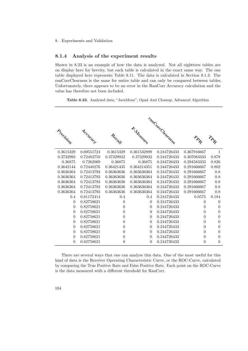
8. Experiments and Validation
8.1.4 Analysis of the experiment resultsShown in 8.23 is an example of how the data is analyzed. Not all eightteen tables areon display here for brevity, but each table is calculated in the exact same way. The onetable displayed here represents Table 8.11. The data is calculated in Section 8.1.3. TheranCorrClearness is the same for entire table and can only be compared between tables.Unfortunately, there appears to be an error in the RanCorr Accuracy calculation and thevalue has therefore not been included.
Table 8.23. Analysed data, “JavaMean”, Opad And Cleanup, Advanced Algorithm
Precision
AccuracyRecall
F-Measure
ranCorrClearnessFPR
TPR
0.3615329 0.69551724 0.3615329 0.361532899 0.244726433 0.367916667 10.3732993 0.72482759 0.37329932 0.37329932 0.244726433 0.307083333 0.878
0.36875 0.7262069 0.36875 0.36875 0.244726433 0.294583333 0.8260.3642144 0.72448276 0.36421435 0.364214351 0.244726433 0.291666667 0.8020.3636364 0.72413793 0.36363636 0.363636364 0.244726433 0.291666667 0.80.3636364 0.72413793 0.36363636 0.363636364 0.244726433 0.291666667 0.80.3636364 0.72413793 0.36363636 0.363636364 0.244726433 0.291666667 0.80.3636364 0.72413793 0.36363636 0.363636364 0.244726433 0.291666667 0.80.3636364 0.72413793 0.36363636 0.363636364 0.244726433 0.291666667 0.8
0.4 0.81172414 0.4 0.4 0.244726433 0.0575 0.1840 0.82758621 0 0 0.244726433 0 00 0.82758621 0 0 0.244726433 0 00 0.82758621 0 0 0.244726433 0 00 0.82758621 0 0 0.244726433 0 00 0.82758621 0 0 0.244726433 0 00 0.82758621 0 0 0.244726433 0 00 0.82758621 0 0 0.244726433 0 00 0.82758621 0 0 0.244726433 0 00 0.82758621 0 0 0.244726433 0 0
There are several ways that one can analyse this data. One of the most useful for thiskind of data is the Receiver Operating Characteristic Curve, or the ROC-Curve, calculatedby comparing the True Positive Rate and False Positive Rate. Each point on the ROC-Curveis the data measured with a different threshold for RanCorr.
104

8.1. Experiments and validation of the Kiekeriki Backend
JavaMean forecasting algorithm results
For the “JavaMean” forecasting algorithm, the following graphs; Figure 8.7, Figure 8.8 andFigure 8.7 represent the quality of each test.
105
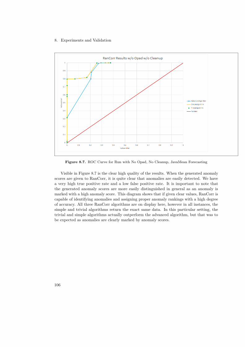
8. Experiments and Validation
Figure 8.7. ROC Curve for Run with No Opad, No Cleanup, JavaMean Forecasting
Visible in Figure 8.7 is the clear high quality of the results. When the generated anomalyscores are given to RanCorr, it is quite clear that anomalies are easily detected. We havea very high true positive rate and a low false positive rate. It is important to note thatthe generated anomaly scores are more easily distinguished in general as an anomaly ismarked with a high anomaly score. This diagram shows that if given clear values, RanCorr iscapable of identifying anomalies and assigning proper anomaly rankings with a high degreeof accuracy. All three RanCorr algorithms are on display here, however in all instances, thesimple and trivial algorithms return the exact same data. In this particular setting, thetrivial and simple algorithms actually outperform the advanced algorithm, but that was tobe expected as anomalies are clearly marked by anomaly scores.
106

8.1. Experiments and validation of the Kiekeriki Backend
Figure 8.8. ROC Curve for Run with Opad, No Cleanup, JavaMean Forecasting
Figure 8.8 shows a clear drop in accuracy in comparison to the data that is generatedwithout ΘPADx. Much of the data is actually on the 0 line for true positive rate, meaningthat none of the injected anomalies were actually detected. Only after the threshold is sethigh enough does the true positive rate eventually rise over the line indicating random chance.This is attributed to the fact that without cleanup, ΘPADx returns a dataset with a latencyof 0 and an anomaly score of 1 for each timeframe in which a method is not detected. Whilethis is in fact desired to capture the anomaly of a program not running at all anymore, itdoes significantly skew our results. Therefore, for Figure 8.7 the data has been sanitized byremoving these sets of data. Also of note here is that all three of the algorithms performequally poor under this setup.
107
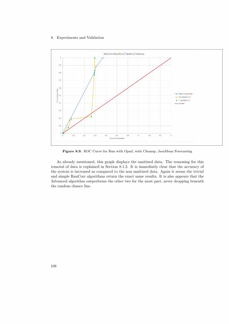
8. Experiments and Validation
Figure 8.9. ROC Curve for Run with Opad, with Cleanup, JavaMean Forecasting
As already mentioned, this graph displays the sanitized data. The reasoning for thisremoval of data is explained in Section 8.1.2. It is immediatly clear that the accuracy ofthe system is increased as compared to the non sanitized data. Again it seems the trivialand simple RanCorr algorithms return the exact same results. It is also appears that theAdvanced algorithm outperforms the other two for the most part, never dropping beneaththe random chance line.
108

8.1. Experiments and validation of the Kiekeriki Backend
Also a relevant comparison is the RanCorrClearness as defined in Section 8.1.3.
Table 8.24. RanCorr Clearness
Path Algorithm RanCorr ClearnessNo Opad No Cleanup Advanced Algorithm 0.259349077
Simple Algorithm 0.330827808Trivial Algorithm 0.330827808
Opad No Cleanup Advanced Algorithm 0.265431363Simple Algorithm 0.277243307Trivial Algorithm 0.277243307
Opad with Cleanup Advanced Algorithm 0.242408967Simple Algorithm 0.275840536Trivial Algorithm 0.275840536
As can be seen, in each case the RanCorr accuracy is lower for the advanced algorithmthan for the others, and the other two are again identical. The clearness is a measure takenfrom Marwede et al. [2009].
109
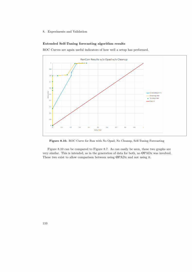
8. Experiments and Validation
Extended Self-Tuning forecasting algorithm results
ROC Curves are again useful indicators of how well a setup has performed.
Figure 8.10. ROC Curve for Run with No Opad, No Cleanup, Self-Tuning Forecasting
Figure 8.10 can be compared to Figure 8.7. As can easily be seen, these two graphs arevery similar. This is intended, as in the generation of data for both, no ΘPADx was involved.These two exist to allow comparison between using ΘPADx and not using it.
110
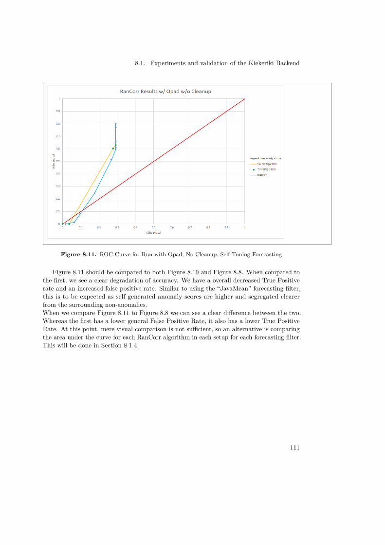
8.1. Experiments and validation of the Kiekeriki Backend
Figure 8.11. ROC Curve for Run with Opad, No Cleanup, Self-Tuning Forecasting
Figure 8.11 should be compared to both Figure 8.10 and Figure 8.8. When compared tothe first, we see a clear degradation of accuracy. We have a overall decreased True Positiverate and an increased false positive rate. Similar to using the “JavaMean” forecasting filter,this is to be expected as self generated anomaly scores are higher and segregated clearerfrom the surrounding non-anomalies.When we compare Figure 8.11 to Figure 8.8 we can see a clear difference between the two.Whereas the first has a lower general False Positive Rate, it also has a lower True PositiveRate. At this point, mere visual comparison is not sufficient, so an alternative is comparingthe area under the curve for each RanCorr algorithm in each setup for each forecasting filter.This will be done in Section 8.1.4.
111
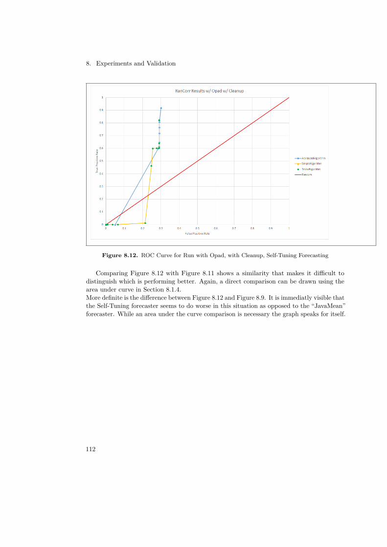
8. Experiments and Validation
Figure 8.12. ROC Curve for Run with Opad, with Cleanup, Self-Tuning Forecasting
Comparing Figure 8.12 with Figure 8.11 shows a similarity that makes it difficult todistinguish which is performing better. Again, a direct comparison can be drawn using thearea under curve in Section 8.1.4.More definite is the difference between Figure 8.12 and Figure 8.9. It is immediatly visible thatthe Self-Tuning forecaster seems to do worse in this situation as opposed to the “JavaMean”forecaster. While an area under the curve comparison is necessary the graph speaks for itself.
112
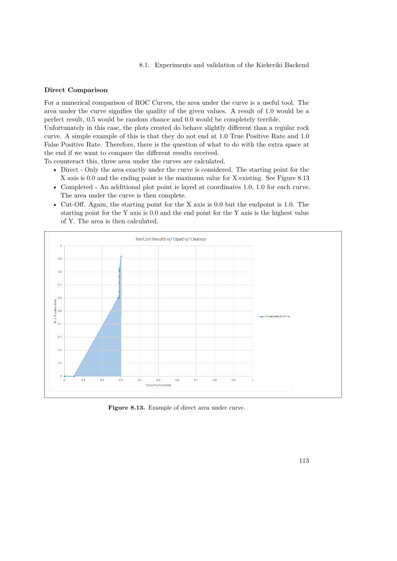
8.1. Experiments and validation of the Kiekeriki Backend
Direct Comparison
For a numerical comparison of ROC Curves, the area under the curve is a useful tool. Thearea under the curve signifies the quality of the given values. A result of 1.0 would be aperfect result, 0.5 would be random chance and 0.0 would be completely terrible.Unfortunately in this case, the plots created do behave slightly different than a regular rockcurve. A simple example of this is that they do not end at 1.0 True Positive Rate and 1.0False Positive Rate. Therefore, there is the question of what to do with the extra space atthe end if we want to compare the different results received.To counteract this, three area under the curves are calculated.
• Direct - Only the area exactly under the curve is considered. The starting point for theX axis is 0.0 and the ending point is the maximum value for X existing. See Figure 8.13
• Completed - An additional plot point is layed at coordinates 1.0, 1.0 for each curve.The area under the curve is then complete.
• Cut-Off. Again, the starting point for the X axis is 0.0 but the endpoint is 1.0. Thestarting point for the Y axis is 0.0 and the end point for the Y axis is the highest valueof Y. The area is then calculated.
Figure 8.13. Example of direct area under curve.
113
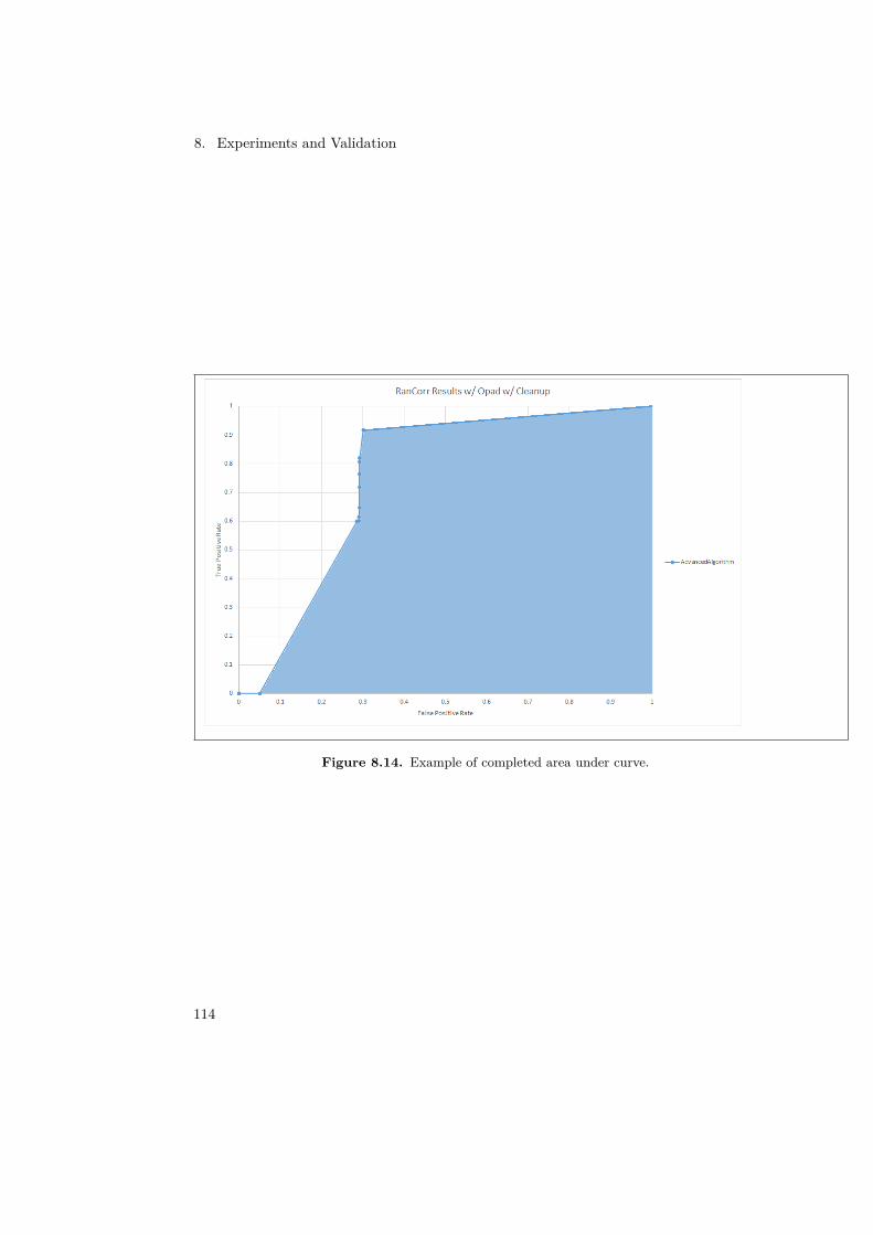
8. Experiments and Validation
Figure 8.14. Example of completed area under curve.
114
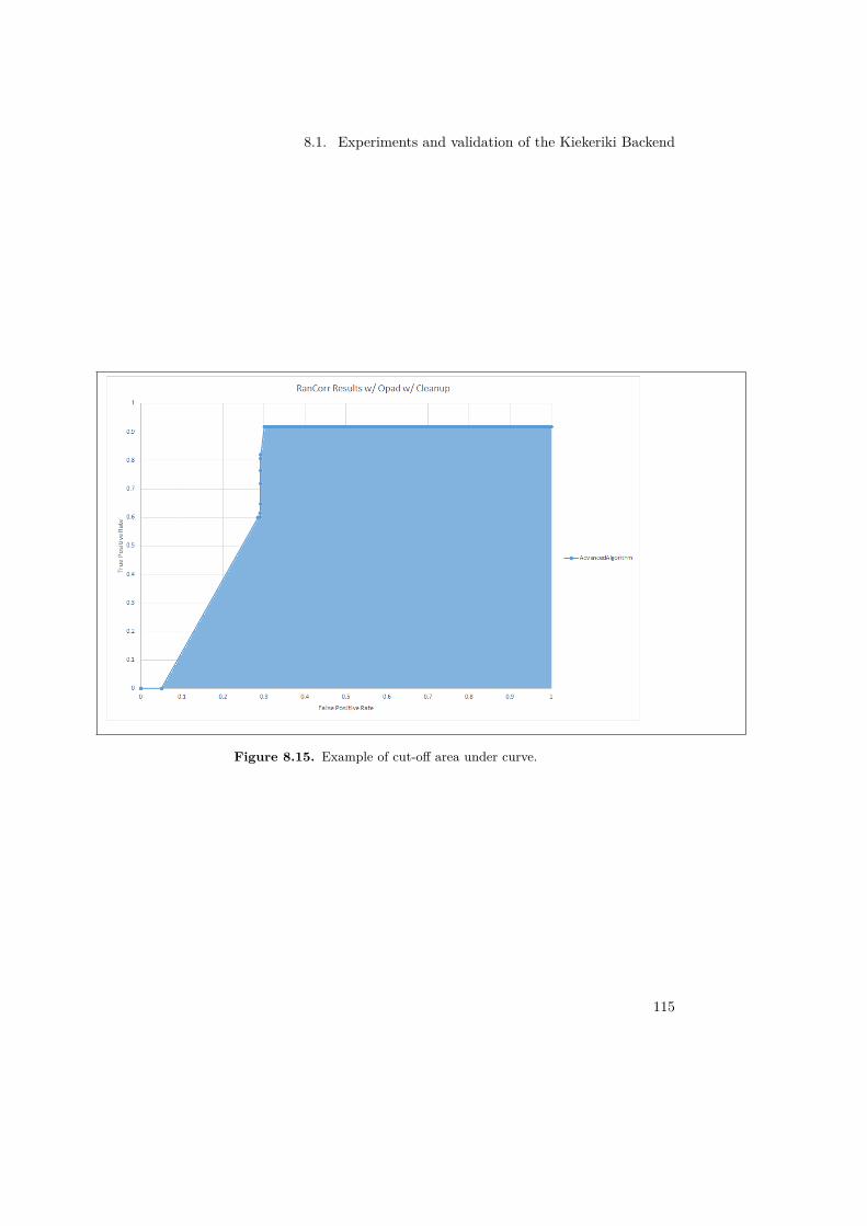
8.1. Experiments and validation of the Kiekeriki Backend
Figure 8.15. Example of cut-off area under curve.
115
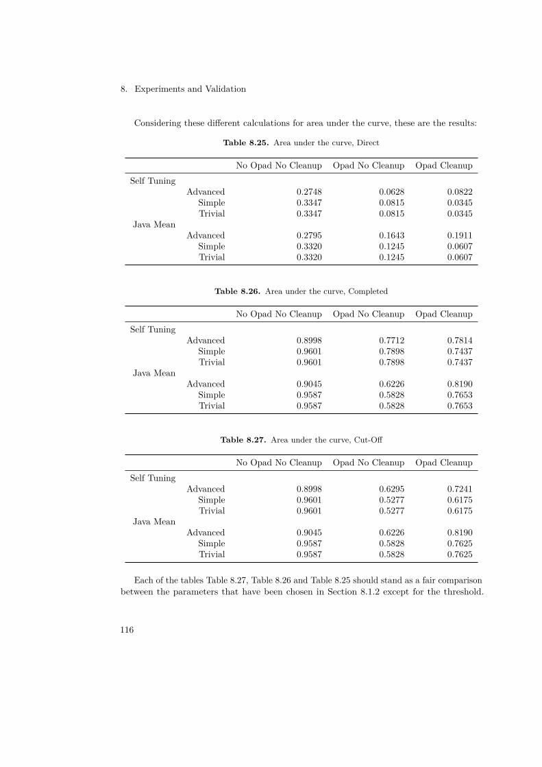
8. Experiments and Validation
Considering these different calculations for area under the curve, these are the results:
Table 8.25. Area under the curve, Direct
No Opad No Cleanup Opad No Cleanup Opad CleanupSelf Tuning
Advanced 0.2748 0.0628 0.0822Simple 0.3347 0.0815 0.0345Trivial 0.3347 0.0815 0.0345
Java MeanAdvanced 0.2795 0.1643 0.1911
Simple 0.3320 0.1245 0.0607Trivial 0.3320 0.1245 0.0607
Table 8.26. Area under the curve, Completed
No Opad No Cleanup Opad No Cleanup Opad CleanupSelf Tuning
Advanced 0.8998 0.7712 0.7814Simple 0.9601 0.7898 0.7437Trivial 0.9601 0.7898 0.7437
Java MeanAdvanced 0.9045 0.6226 0.8190
Simple 0.9587 0.5828 0.7653Trivial 0.9587 0.5828 0.7653
Table 8.27. Area under the curve, Cut-Off
No Opad No Cleanup Opad No Cleanup Opad CleanupSelf Tuning
Advanced 0.8998 0.6295 0.7241Simple 0.9601 0.5277 0.6175Trivial 0.9601 0.5277 0.6175
Java MeanAdvanced 0.9045 0.6226 0.8190
Simple 0.9587 0.5828 0.7625Trivial 0.9587 0.5828 0.7625
Each of the tables Table 8.27, Table 8.26 and Table 8.25 should stand as a fair comparisonbetween the parameters that have been chosen in Section 8.1.2 except for the threshold.
116
8.1. Experiments and validation of the Kiekeriki Backend
The threshold is contained within each of these results already and is iterated over in anidentical fashion in each individual result. Represented are the path chosen (as described inSection 8.1.2), the forecasting algorithms and the RanCorr algorithms.What should be noted is that the “Direct” approach to the area under the curve does notgive us a useful result. In a ROC curve, an area under the curve of 0.5 is considered the bethe score that a random choice algorithm would score. Yet, despite that in the diagrams itcan cleary be seen that the results are significantly over the random line, the score in the“Direct” area under the curve measurement does not reflect this in Table 8.25. Therefore thisis not a useful measurement.The “Cut-Off” method delivers what can be considered the worst case scenario. If futuremeasurements delivered results that would only increase the False Positive Rate with a staticTrue Positive Rate. The alternative would be the best scenario, where the True PositiveRate would climb to one without the False Positive Rate increasing.Therefore, the “Completed” method would deliver an average result, between best and worstcase, where both the True Positive and the False Positive rates approached 1.0. We canconsider both the “Completed” and the “Cut-Off” methods to return useful data.
Christopher Gregorian
117
8. Experiments and Validation
8.1.5 Conclusion
The goal of the entire experiment setup was to answer the questions posed in Section 8.1.1.Therefore it is fitting to look how our results answer each individual question.
Question 1.1
How well does Kiekeriki find injected anomalies?To discuss the quality of anomaly detection, one should turn to the area under the curvemethod. Table 8.26 and Table 8.27 display values for several areas under the curve.When no ΘPADx is used at all, the area under the curve stands near or above 0.9, showinga very good result. When ΘPADx is generating anomaly scores, a marked drop in results isclearly visible. In the worst case (Cut-Off area under the curve Table 8.27) the result standsbetween 0.52 and 0.63 at a score much closer to random. This is a very poor result andstems mostly from the fact that, as discussed in Section 8.1.2, ΘPADx will generate highanomaly scores of 1.0 for times when a method is not detected at all.However, when these anomalies are removed (under “Opad Cleanup”) and only the intendedanomalies remain, the detection rate climbs quite steadily. From 0.61 in the worst case to 0.81.Und what is considered an average case, the result is between 0.74 and 0.81 (Table 8.26).By assessing these results, it is clear that Kiekeriki can detect anomalies quite well andthe low scores under “Opad No Cleanup” stem not from Kiekeriki itself, but from a knownproblem with the data generation.
Question 1.2
How does the RanCorr algorithm type affect the output?One of the most obvious conclusion that can be drawn is that apparently the Simple andTrivial algorithms are not in any way different. Whether this is a flaw in the algorithmsthemselves, the data generation or the implementation is unknown. The results however areidentical for every single run.As for the difference between the Advanced algorithm and the others it is again necessary tolook at the worst case scenario Table 8.27. It is shown that when no ΘPADx is running, theSimple/Trivial algorithms outperform the Advanced algorithm by a margin of 0.06 or 6%.However, once ΘPADxis used in either its native or cleaned up form, the Advanced algorithmoutperforms its counterpats by 10% or more. In the average case (Table 8.26) the differencebecomes more subtle with only 3.7%. The conclusions that can be drawn are quite simple.The implementations of the Trivial and Simple algorithms will perform exactly identicaleach time and in the relevant scenario (ΘPADx creating data) the Advanced algorithm willoutperform the others by a sizeable margin or be just about equal in performance.
118
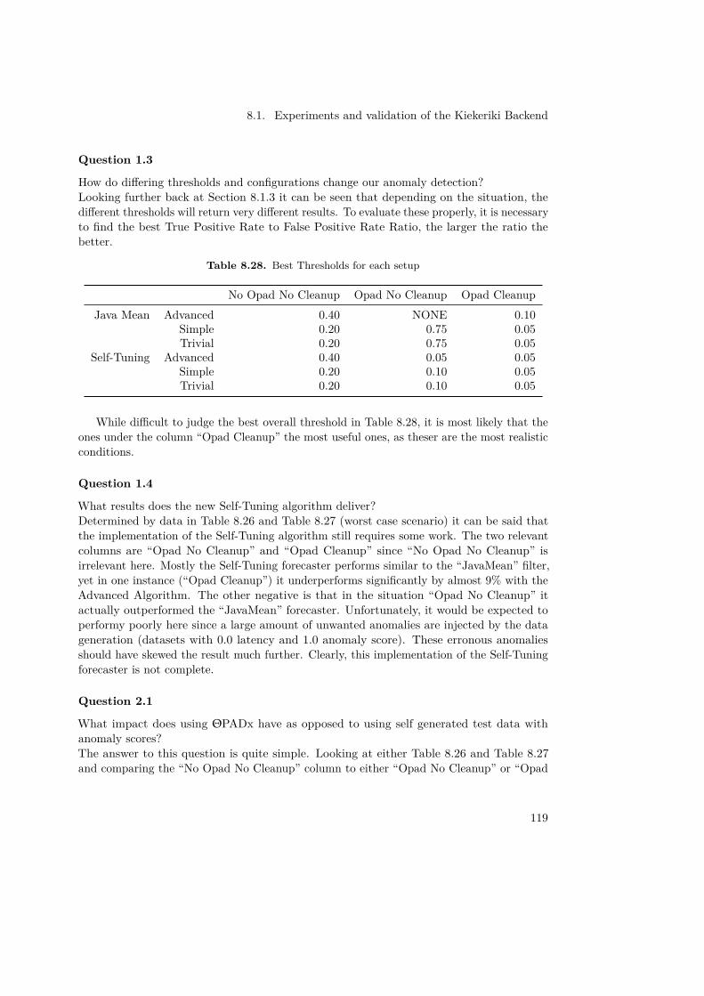
8.1. Experiments and validation of the Kiekeriki Backend
Question 1.3
How do differing thresholds and configurations change our anomaly detection?Looking further back at Section 8.1.3 it can be seen that depending on the situation, thedifferent thresholds will return very different results. To evaluate these properly, it is necessaryto find the best True Positive Rate to False Positive Rate Ratio, the larger the ratio thebetter.
Table 8.28. Best Thresholds for each setup
No Opad No Cleanup Opad No Cleanup Opad CleanupJava Mean Advanced 0.40 NONE 0.10
Simple 0.20 0.75 0.05Trivial 0.20 0.75 0.05
Self-Tuning Advanced 0.40 0.05 0.05Simple 0.20 0.10 0.05Trivial 0.20 0.10 0.05
While difficult to judge the best overall threshold in Table 8.28, it is most likely that theones under the column “Opad Cleanup” the most useful ones, as theser are the most realisticconditions.
Question 1.4
What results does the new Self-Tuning algorithm deliver?Determined by data in Table 8.26 and Table 8.27 (worst case scenario) it can be said thatthe implementation of the Self-Tuning algorithm still requires some work. The two relevantcolumns are “Opad No Cleanup” and “Opad Cleanup” since “No Opad No Cleanup” isirrelevant here. Mostly the Self-Tuning forecaster performs similar to the “JavaMean” filter,yet in one instance (“Opad Cleanup”) it underperforms significantly by almost 9% with theAdvanced Algorithm. The other negative is that in the situation “Opad No Cleanup” itactually outperformed the “JavaMean” forecaster. Unfortunately, it would be expected toperformy poorly here since a large amount of unwanted anomalies are injected by the datageneration (datasets with 0.0 latency and 1.0 anomaly score). These erronous anomaliesshould have skewed the result much further. Clearly, this implementation of the Self-Tuningforecaster is not complete.
Question 2.1
What impact does using ΘPADx have as opposed to using self generated test data withanomaly scores?The answer to this question is quite simple. Looking at either Table 8.26 and Table 8.27and comparing the “No Opad No Cleanup” column to either “Opad No Cleanup” or “Opad
119
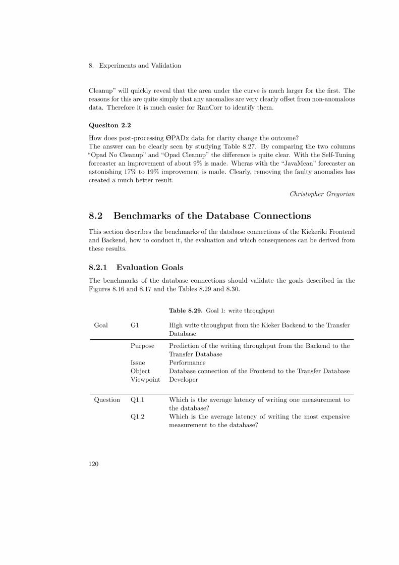
8. Experiments and Validation
Cleanup” will quickly reveal that the area under the curve is much larger for the first. Thereasons for this are quite simply that any anomalies are very clearly offset from non-anomalousdata. Therefore it is much easier for RanCorr to identify them.
Quesiton 2.2
How does post-processing ΘPADx data for clarity change the outcome?The answer can be clearly seen by studying Table 8.27. By comparing the two columns“Opad No Cleanup” and “Opad Cleanup” the difference is quite clear. With the Self-Tuningforecaster an improvement of about 9% is made. Wheras with the “JavaMean” forecaster anastonishing 17% to 19% improvement is made. Clearly, removing the faulty anomalies hascreated a much better result.
Christopher Gregorian
8.2 Benchmarks of the Database ConnectionsThis section describes the benchmarks of the database connections of the Kiekeriki Frontendand Backend, how to conduct it, the evaluation and which consequences can be derived fromthese results.
8.2.1 Evaluation GoalsThe benchmarks of the database connections should validate the goals described in theFigures 8.16 and 8.17 and the Tables 8.29 and 8.30.
Table 8.29. Goal 1: write throughput
Goal G1 High write throughput from the Kieker Backend to the TransferDatabase
Purpose Prediction of the writing throughput from the Backend to theTransfer Database
Issue PerformanceObject Database connection of the Frontend to the Transfer DatabaseViewpoint Developer
Question Q1.1 Which is the average latency of writing one measurement tothe database?
Q1.2 Which is the average latency of writing the most expensivemeasurement to the database?
120
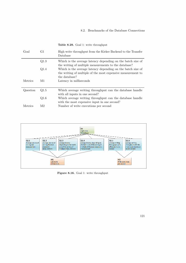
8.2. Benchmarks of the Database Connections
Table 8.29. Goal 1: write throughput
Goal G1 High write throughput from the Kieker Backend to the TransferDatabase
Q1.3 Which is the average latency depending on the batch size ofthe writing of multiple measurements to the database?
Q1.4 Which is the average latency depending on the batch size ofthe writing of multiple of the most expensive measurement tothe database?
Metrics M1 Latency in milliseconds
Question Q1.5 Which average writing throughput can the database handlewith all inputs in one second?
Q1.6 Which average writing throughput can the database handlewith the most expensive input in one second?
Metrics M2 Number of write executions per second
Figure 8.16. Goal 1: write throughput
121
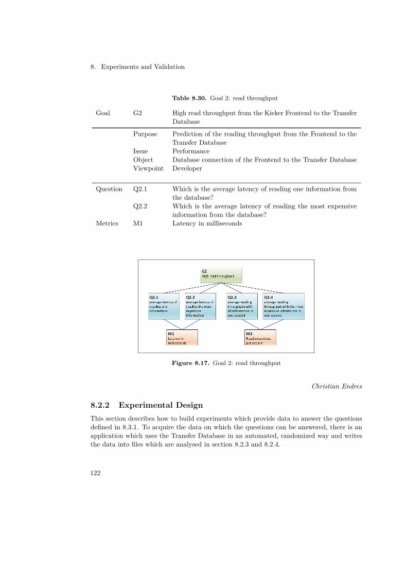
8. Experiments and Validation
Table 8.30. Goal 2: read throughput
Goal G2 High read throughput from the Kieker Frontend to the TransferDatabase
Purpose Prediction of the reading throughput from the Frontend to theTransfer Database
Issue PerformanceObject Database connection of the Frontend to the Transfer DatabaseViewpoint Developer
Question Q2.1 Which is the average latency of reading one information fromthe database?
Q2.2 Which is the average latency of reading the most expensiveinformation from the database?
Metrics M1 Latency in milliseconds
Figure 8.17. Goal 2: read throughput
Christian Endres
8.2.2 Experimental DesignThis section describes how to build experiments which provide data to answer the questionsdefined in 8.3.1. To acquire the data on which the questions can be answered, there is anapplication which uses the Transfer Database in an automated, randomized way and writesthe data into files which are analysed in section 8.2.3 and 8.2.4.
122
8.2. Benchmarks of the Database Connections
Hardware setup
The project uses a server at the data center of the Hetzner Online AG for the experiments.The Hetzner server has an IntelrCore i7-920 Quadcore processor, 48 GB DDR3 RAM andtwo 2 TB SATA 3Gb/s Enterprise HDDs in a raid 1 configuration.
Software setup
The Hetzner server runs a Debian 3.2.51-1 x86_64 GNU/Linux, Java version 1.7.0_51 and aMySQL-Server 5.5.35.
Experimental setup
To answer the questions of 8.3.1, there is a load driver (see 7.4) which stresses the database.The load driver uses one connection to the database and has the (slightly adjusted) methodsof the Kieker Backend and the Kieker Frontend. The load driver is executed on the sameHetzner server as the Transfer database and the application server on which the KiekerFrontend is running.
Benchmark execution
For the execution of the benchmarks the KiekerTransferDBDataGenerator uses a bench-marking framework [Boyer, 2008a,b,c] which agrees with [Georges et al., 2007] about howto conduct statistically rigorous benchmarks of Java applications. The framework cares foreverything like the heating phase before the measurements for example. A benchmark exe-cutes exactly 60 measurements rounds with multiple single measurements each round. If thecompiling time differs, the benchmark framework restarts and starts another 60 measurementrounds until all runs without any cause for restart again.
Christian Endres
8.2.3 Analysis of the Benchmark Results for the Kiekeriki BackendFigure 8.18 shows the latencies of each method which writes to the Transfer Database. Eachmethod has many outliers which can be even 10 times higher than the median. This can bea result of many different system behaviors which the benchmark was still prone to. Thusthe questions Q1.1 cannot be answered definitely. Question Q1.2 asks for the most expensivewrite operation, which cannot be determined, too. The medians of each writing method arenearly the same and the box plots show that the second and third percentiles are overlapping.
The question Q1.3 can be answered for higher batch sizes by the Figure 8.19 and Table 8.31,though the measurements are prone to the outliers. This is the result of the high standarddeviation of the write executions as learned from the single write benchmarks. The values ofthe column set “Mean per data set” indicates a decreasing mean execution time per data setfor increasing batch size. Though the measurements with a batch size of 50 contradicts. The
123
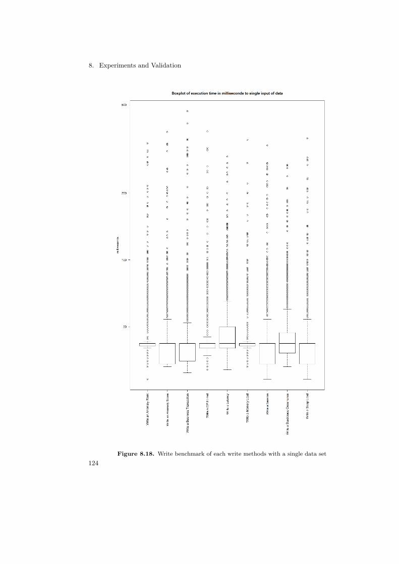
8. Experiments and Validation
Figure 8.18. Write benchmark of each write methods with a single data set124
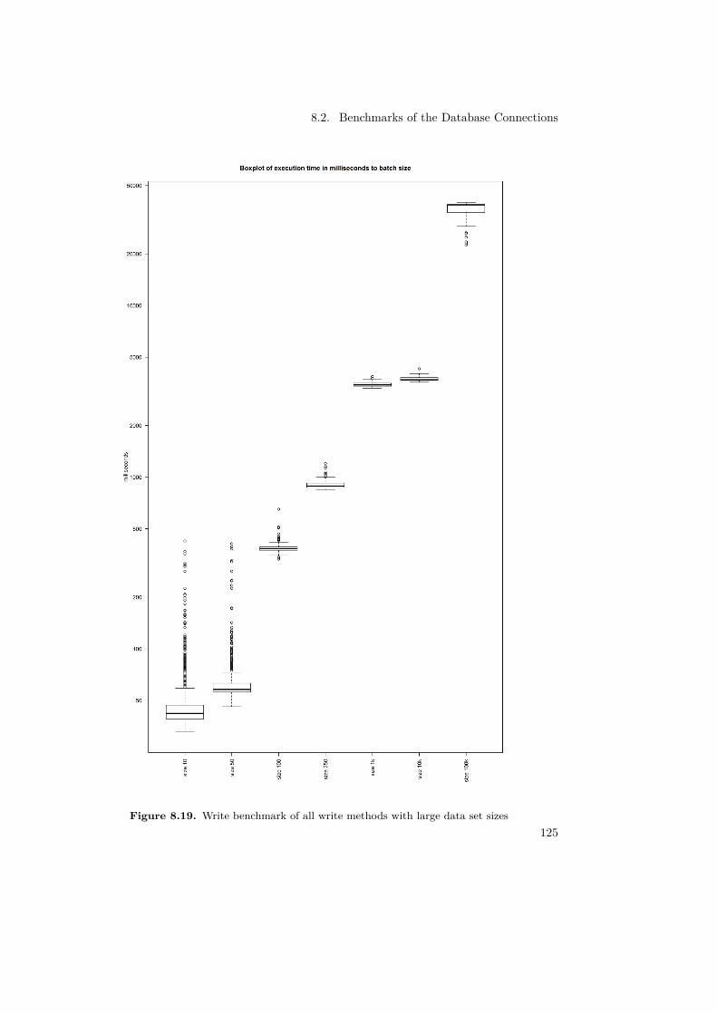
8.2. Benchmarks of the Database Connections
Figure 8.19. Write benchmark of all write methods with large data set sizes125
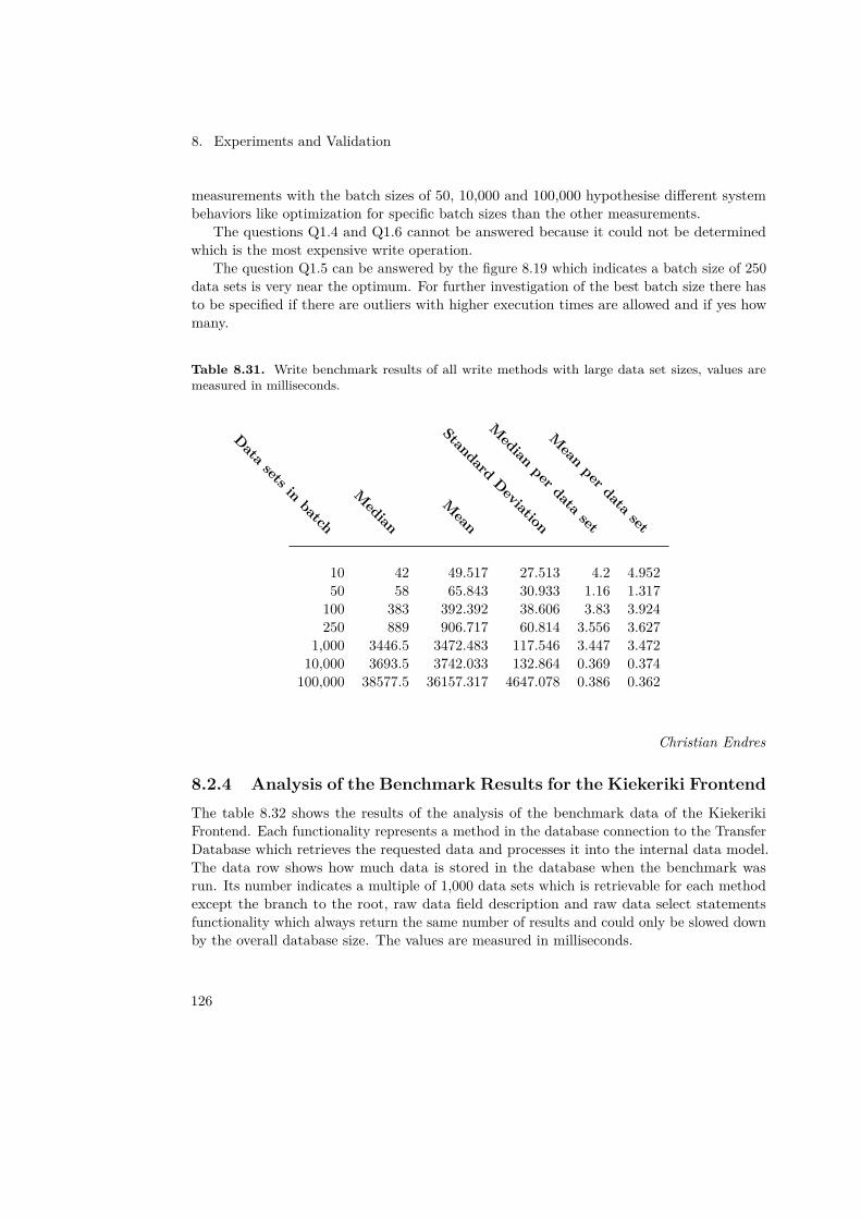
8. Experiments and Validation
measurements with the batch sizes of 50, 10,000 and 100,000 hypothesise different systembehaviors like optimization for specific batch sizes than the other measurements.
The questions Q1.4 and Q1.6 cannot be answered because it could not be determinedwhich is the most expensive write operation.
The question Q1.5 can be answered by the figure 8.19 which indicates a batch size of 250data sets is very near the optimum. For further investigation of the best batch size there hasto be specified if there are outliers with higher execution times are allowed and if yes howmany.
Table 8.31. Write benchmark results of all write methods with large data set sizes, values aremeasured in milliseconds.
Data sets inbatch
Median
Mean
StandardDeviation
Median
per data set
Mean
per data set
10 42 49.517 27.513 4.2 4.95250 58 65.843 30.933 1.16 1.317
100 383 392.392 38.606 3.83 3.924250 889 906.717 60.814 3.556 3.627
1,000 3446.5 3472.483 117.546 3.447 3.47210,000 3693.5 3742.033 132.864 0.369 0.374
100,000 38577.5 36157.317 4647.078 0.386 0.362
Christian Endres
8.2.4 Analysis of the Benchmark Results for the Kiekeriki FrontendThe table 8.32 shows the results of the analysis of the benchmark data of the KiekerikiFrontend. Each functionality represents a method in the database connection to the TransferDatabase which retrieves the requested data and processes it into the internal data model.The data row shows how much data is stored in the database when the benchmark wasrun. Its number indicates a multiple of 1,000 data sets which is retrievable for each methodexcept the branch to the root, raw data field description and raw data select statementsfunctionality which always return the same number of results and could only be slowed downby the overall database size. The values are measured in milliseconds.
126
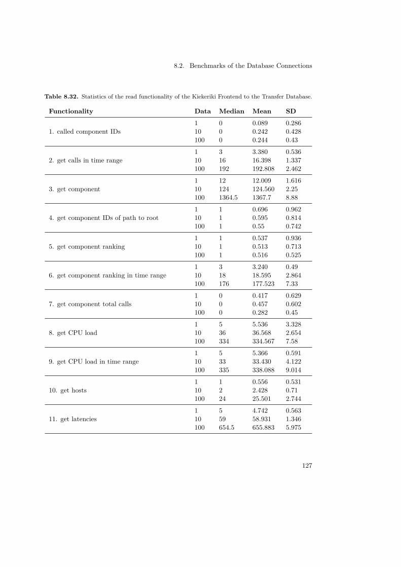
8.2. Benchmarks of the Database Connections
Table 8.32. Statistics of the read functionality of the Kiekeriki Frontend to the Transfer Database.
Functionality Data Median Mean SD
1. called component IDs1 0 0.089 0.28610 0 0.242 0.428100 0 0.244 0.43
2. get calls in time range1 3 3.380 0.53610 16 16.398 1.337100 192 192.808 2.462
3. get component1 12 12.009 1.61610 124 124.560 2.25100 1364.5 1367.7 8.88
4. get component IDs of path to root1 1 0.696 0.96210 1 0.595 0.814100 1 0.55 0.742
5. get component ranking1 1 0.537 0.93610 1 0.513 0.713100 1 0.516 0.525
6. get component ranking in time range1 3 3.240 0.4910 18 18.595 2.864100 176 177.523 7.33
7. get component total calls1 0 0.417 0.62910 0 0.457 0.602100 0 0.282 0.45
8. get CPU load1 5 5.536 3.32810 36 36.568 2.654100 334 334.567 7.58
9. get CPU load in time range1 5 5.366 0.59110 33 33.430 4.122100 335 338.088 9.014
10. get hosts1 1 0.556 0.53110 2 2.428 0.71100 24 25.501 2.744
11. get latencies1 5 4.742 0.56310 59 58.931 1.346100 654.5 655.883 5.975
127
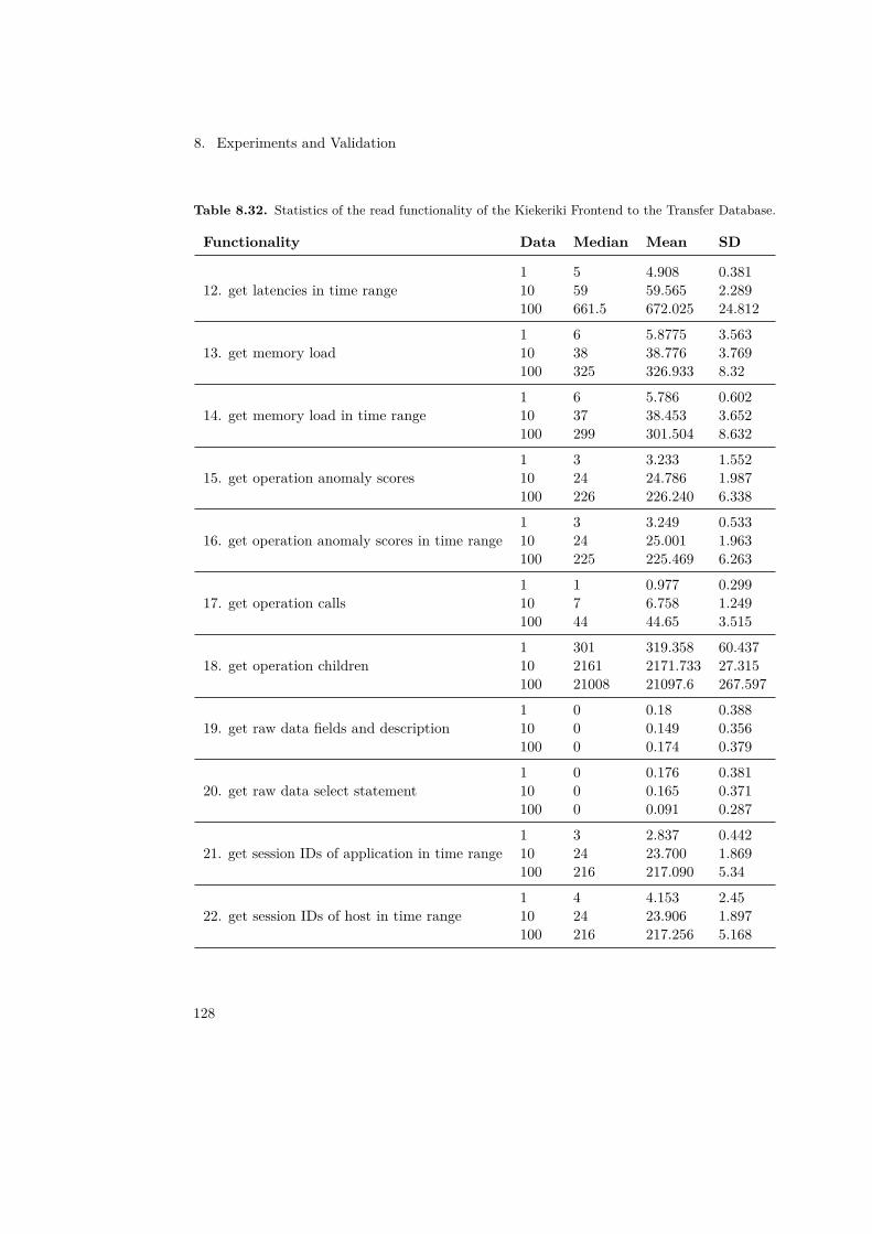
8. Experiments and Validation
Table 8.32. Statistics of the read functionality of the Kiekeriki Frontend to the Transfer Database.
Functionality Data Median Mean SD
12. get latencies in time range1 5 4.908 0.38110 59 59.565 2.289100 661.5 672.025 24.812
13. get memory load1 6 5.8775 3.56310 38 38.776 3.769100 325 326.933 8.32
14. get memory load in time range1 6 5.786 0.60210 37 38.453 3.652100 299 301.504 8.632
15. get operation anomaly scores1 3 3.233 1.55210 24 24.786 1.987100 226 226.240 6.338
16. get operation anomaly scores in time range1 3 3.249 0.53310 24 25.001 1.963100 225 225.469 6.263
17. get operation calls1 1 0.977 0.29910 7 6.758 1.249100 44 44.65 3.515
18. get operation children1 301 319.358 60.43710 2161 2171.733 27.315100 21008 21097.6 267.597
19. get raw data fields and description1 0 0.18 0.38810 0 0.149 0.356100 0 0.174 0.379
20. get raw data select statement1 0 0.176 0.38110 0 0.165 0.371100 0 0.091 0.287
21. get session IDs of application in time range1 3 2.837 0.44210 24 23.700 1.869100 216 217.090 5.34
22. get session IDs of host in time range1 4 4.153 2.4510 24 23.906 1.897100 216 217.256 5.168
128
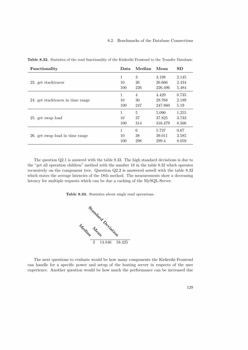
8.2. Benchmarks of the Database Connections
Table 8.32. Statistics of the read functionality of the Kiekeriki Frontend to the Transfer Database.
Functionality Data Median Mean SD
23. get stacktraces1 3 3.198 2.14510 26 26.666 2.434100 226 226.496 5.484
24. get stacktraces in time range1 4 4.429 0.73510 30 29.768 2.189100 247 247.860 5.19
25. get swap load1 5 5.090 1.25510 37 37.825 3.733100 314 316.479 8.566
26. get swap load in time range1 6 5.737 0.6710 38 39.011 3.585100 298 299.4 8.059
The question Q2.1 is answerd with the table 8.33. The high standard deviations is due tothe “get all operation children” method with the number 18 in the table 8.32 which operatesrecursively on the component tree. Question Q2.2 is answered aswell with the table 8.32which states the average latencies of the 18th method. The measurements show a decreasinglatency for multiple requests which can be due a caching of the MySQL-Server.
Table 8.33. Statistics about single read operations.
Median
Mean
StandardDeviation
3 14.846 58.425
The next questions to evaluate would be how many components the Kiekeriki Frontendcan handle for a specific power and setup of the hosting server in respects of the userexperience. Another question would be how much the performance can be increased due
129
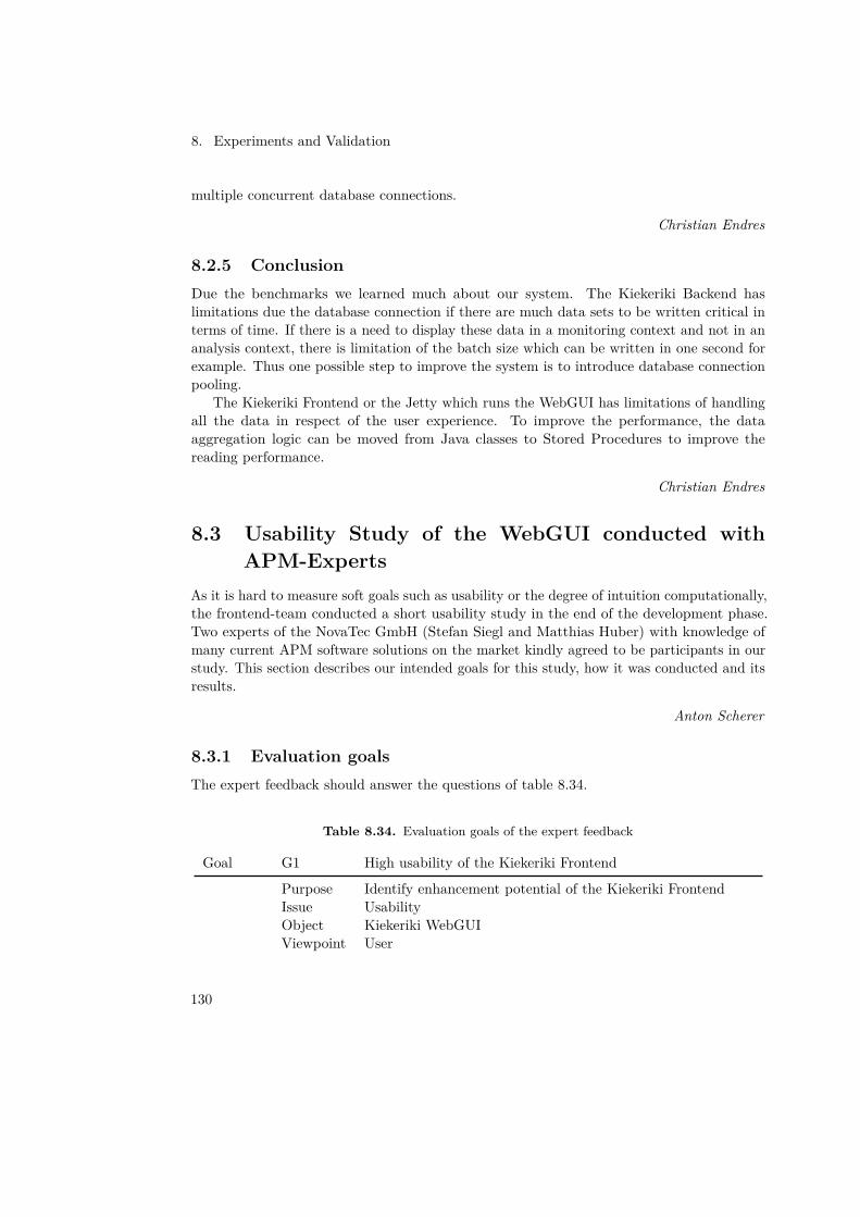
8. Experiments and Validation
multiple concurrent database connections.
Christian Endres
8.2.5 ConclusionDue the benchmarks we learned much about our system. The Kiekeriki Backend haslimitations due the database connection if there are much data sets to be written critical interms of time. If there is a need to display these data in a monitoring context and not in ananalysis context, there is limitation of the batch size which can be written in one second forexample. Thus one possible step to improve the system is to introduce database connectionpooling.
The Kiekeriki Frontend or the Jetty which runs the WebGUI has limitations of handlingall the data in respect of the user experience. To improve the performance, the dataaggregation logic can be moved from Java classes to Stored Procedures to improve thereading performance.
Christian Endres
8.3 Usability Study of the WebGUI conducted withAPM-Experts
As it is hard to measure soft goals such as usability or the degree of intuition computationally,the frontend-team conducted a short usability study in the end of the development phase.Two experts of the NovaTec GmbH (Stefan Siegl and Matthias Huber) with knowledge ofmany current APM software solutions on the market kindly agreed to be participants in ourstudy. This section describes our intended goals for this study, how it was conducted and itsresults.
Anton Scherer
8.3.1 Evaluation goalsThe expert feedback should answer the questions of table 8.34.
Table 8.34. Evaluation goals of the expert feedback
Goal G1 High usability of the Kiekeriki Frontend
Purpose Identify enhancement potential of the Kiekeriki FrontendIssue UsabilityObject Kiekeriki WebGUIViewpoint User
130
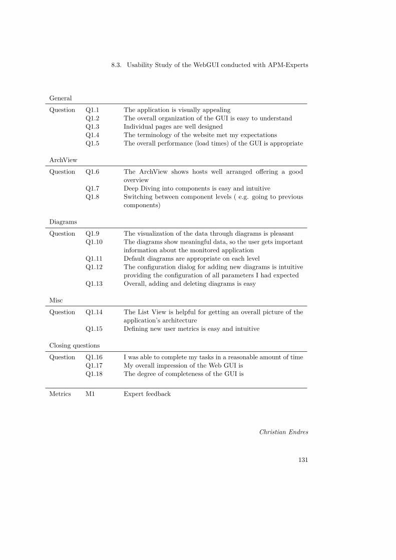
8.3. Usability Study of the WebGUI conducted with APM-Experts
General
Question Q1.1 The application is visually appealingQ1.2 The overall organization of the GUI is easy to understandQ1.3 Individual pages are well designedQ1.4 The terminology of the website met my expectationsQ1.5 The overall performance (load times) of the GUI is appropriate
ArchView
Question Q1.6 The ArchView shows hosts well arranged offering a goodoverview
Q1.7 Deep Diving into components is easy and intuitiveQ1.8 Switching between component levels ( e.g. going to previous
components)
Diagrams
Question Q1.9 The visualization of the data through diagrams is pleasantQ1.10 The diagrams show meaningful data, so the user gets important
information about the monitored applicationQ1.11 Default diagrams are appropriate on each levelQ1.12 The configuration dialog for adding new diagrams is intuitive
providing the configuration of all parameters I had expectedQ1.13 Overall, adding and deleting diagrams is easy
Misc
Question Q1.14 The List View is helpful for getting an overall picture of theapplication’s architecture
Q1.15 Defining new user metrics is easy and intuitive
Closing questions
Question Q1.16 I was able to complete my tasks in a reasonable amount of timeQ1.17 My overall impression of the Web GUI isQ1.18 The degree of completeness of the GUI is
Metrics M1 Expert feedback
Christian Endres
131
8. Experiments and Validation
8.3.2 Conducting the usability testAccording to a lecture of the University of Washington ([?]), a typical usability test consistsof the four main steps we complied with in our study:
1. Find representative usersSince the WebGUI is not designed to be used by standard end users but system adminis-trators, experts are necessary for our study. Because APM experts are expected to have agreat knowledge about how a monitoring WebGUI is structured, they are able to give aqualified feedback. Furthermore, if they have problems using specific features of the GUI,it is highly probable that the majority will not get this feature to work correctly.
2. Ask the users to perform representative tasksFor this step, the frontend-team (represented by Christian Endres and Anton Scherer)prepared some use cases the participants had to go through. For this purpose, theunderlying database was prepared to contain synthetical data, where the use cases canbe conducted on. However, before the test persons started to interact with the GUI, thefrontend team gave a short introduction about the context, the generated data and theused metrics. After that, the following use cases were given as tasks to be performed:
• Deep dive into any method level• Add an arbitrary diagram showing historical data• Define a new user metric• Create a new diagram that displays the newly defined metric with live data• Create a new diagram which shows the anomaly score of ΘPAD• Change options of an existing diagram• Find an anomaly by showing the matching anomaly rank
After the use cases were executed, the test persons had time to use the GUI in anexplorative way with no restrictions about what they were doing.
3. Oberserve what the users doWhile the two experts were using the web application, their behavoir was carefully analyzedby the examiners. If problems arose during interaction with the GUI, they were writtendown. Also communication between the two test persons was recorded in order to knowwhich sections in the GUI caused unclarity.
4. Get feedback and summarize the resultsMost feedback was given while the test persons were interacting with the WebGUI. Ifquestions arose, they were asked immediately. Often, the experts made improvementsuggestions for the detected weakness points. In addition to the consecutive feedback,the frontend team handed a questionnaire out to the experts containing 18 questions forrating the GUI. We emphasized that this judgement will not affect the project’s rating
132

8.3. Usability Study of the WebGUI conducted with APM-Experts
in order to get honest assessments. The questionnaire’s results are illustrated in 8.3.3.Finally, a last feedback round finished the usability study.
Anton Scherer
8.3.3 Usability Study ResultsThis section reveals the results of the usability study. The experts’ feedback was constructiveas they did not just criticize but also suggest how to do it better. The following tablestructures the feedback the experts gave to optimize the GUI. The frontend team evaluatedthe tasks and decided which of these suggestions can be implemented within a reasonableamount of time. Due to time pressure, we had to reject some tasks which are consideredcomplex. These are referenced in the future work (Chapter 9). All other optimizations wereimplemented in the last sprint.
Category Task Should befixed?
Configure Dialog
Delete the metric ID out of the dialog YesProvide more information in the metricselection
Yes
Find another solution for the metriccaroussell (not intuitive)
No
Line break for description field NoCancel button does not always work NoResizing the window does not work YesPosition and size of the dialog must notoversize the screen
Yes
The time unit selection is not intuitive NoProvide default values in every se-lectable field
No
Explicitly show the level on which thedialog should be added
No
Metrics definition
Place "Add new user metric"-button ontop of the table
Yes
The raw data table must be placed be-low
Yes
Delete the percentile option as it doesnot work correctly
Yes
Define which function makes sense onwhich metric
No
Close the dialog after a new metric wasadded
Yes
133
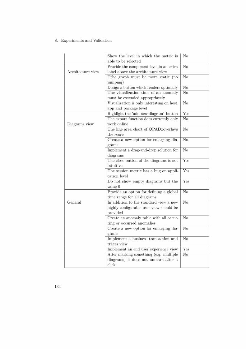
8. Experiments and Validation
Show the level in which the metric isable to be selected
No
Architecture viewProvide the component level in an extralabel above the architecture view
No
Tthe graph must be more static (nojumping)
No
Design a button which renders optimally NoThe visualization time of an anomalymust be extended appropriately
No
Visualization is only interesting on host,app and package level
No
Diagrams view
Highlight the "add new diagram"-button YesThe export function does currently onlywork online
No
The line area chart of ΘPADxoverlaysthe score
No
Create a new option for enlarging dia-grams
No
Implement a drag-and-drop solution fordiagrams
No
The close button of the diagrams is notintuitive
Yes
The session metric has a bug on appli-cation level
Yes
Do not show empty diagrams but thevalue 0
Yes
General
Provide an option for defining a globaltime range for all diagrams
No
In addition to the standard view a newhighly configurable user-view should beprovided
No
Create an anomaly table with all occur-ring or occurred anomalies
No
Create a new option for enlarging dia-grams
No
Implement a business transaction andtraces view
No
Implement an end user experience view YesAfter marking something (e.g. multiplediagrams) it does not unmark after aclick
No
134
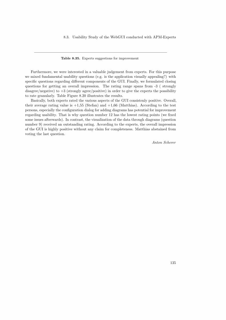
8.3. Usability Study of the WebGUI conducted with APM-Experts
Table 8.35. Experts suggestions for improvement
Furthermore, we were interested in a valuable judgement from experts. For this purposewe mixed fundamental usability questions (e.g. is the application visually appealing?) withspecific questions regarding different components of the GUI. Finally, we formulated closingquestions for getting an overall impression. The rating range spans from -3 ( stronglydisagree/negative) to +3 (strongly agree/positive) in order to give the experts the possibilityto rate granularly. Table Figure 8.20 illustrates the results.
Basically, both experts rated the various aspects of the GUI consistenly positive. Overall,their average rating value is +1,55 (Stefan) and +1,66 (Matthias). According to the testpersons, especially the configuration dialog for adding diagrams has potential for improvementregarding usability. That is why question number 12 has the lowest rating points (we fixedsome issues afterwards). In contrast, the visualization of the data through diagrams (questionnumber 9) received an outstanding rating. According to the experts, the overall impressionof the GUI is highly positive without any claim for completeness. Matthias abstained fromvoting the last question.
Anton Scherer
135
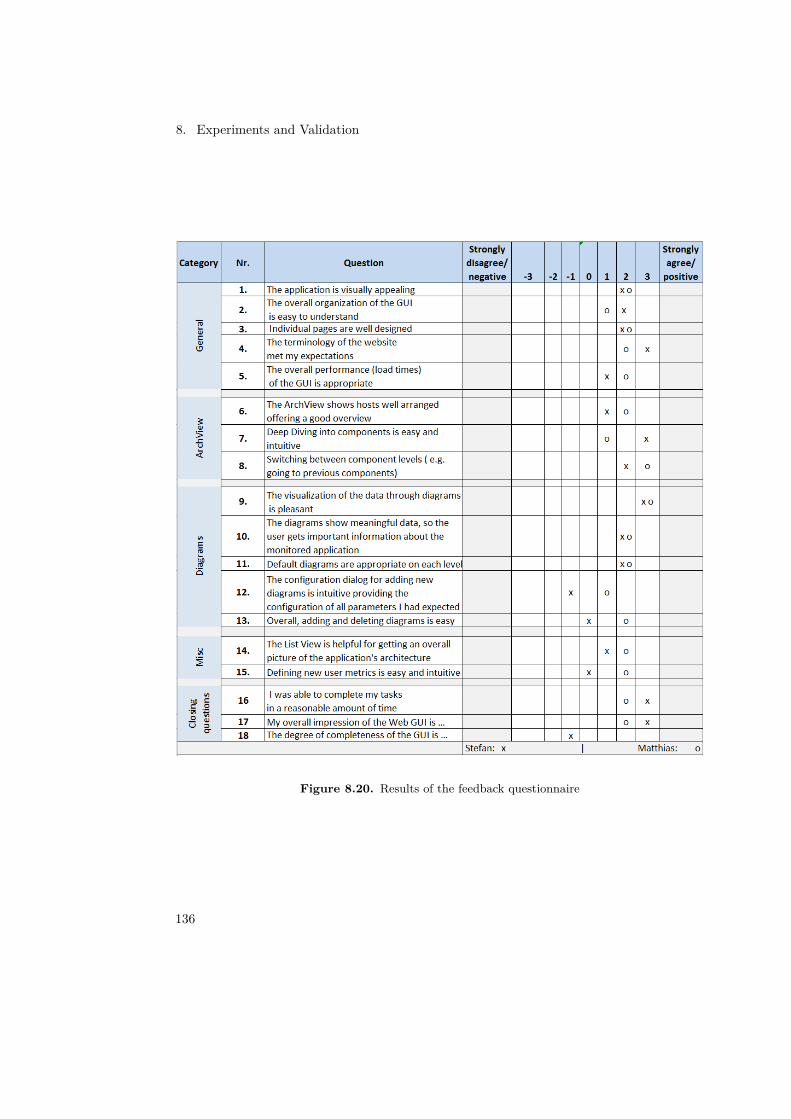
8. Experiments and Validation
Figure 8.20. Results of the feedback questionnaire
136
Chapter 9
Future Work
This chapter considers possible topics for future extension and development of Kieker.
9.1 Backend• ARIMA and GARCH
Extend ΘPAD with a new forecasting algorithm based on ARIMA and GARCHintroduced in Amin et al. [2012].
• Business Transaction DetectionBusiness Transaction Detection tries to detect continuously occuring sequences ofmethods that may represent a business transaction. E. g., a login process.
• Correlation of MeasuresCorrelation of measures tries to identify correlation patterns between two or moreindependet measures taken by Kieker. E. g., increased CPU-load correlates withincreased anomaly scores.
• Software Aging DetectionSoftware aging describes a progressive degredation of performance caused by errors,memory leaks, fragmentation or exhaustion of other resources. Kieker may be extendedto detect symptomps of software aging like continuously increasing latencies. Thiswould basically introduce a new anomaly detection algorithm.
• Exception Monitoring
Exception occuring in the instrumented and observed application can not be recog-nized as such by Kieker. Exception could be registered by Kieker and offered to the GUI.
• ExperimentsThe newly implemented experiment framework features collective, point and contextualanomalies. Not yet implemented are system-wide anomalies, or anomalies caused by acomplete failure of individual components. Provide more complex input generation
137
9. Future Work
patterns and pattern recognition within the output evaluation.
• Online Configuration Kiekeriki is currently not controlled by the GUI. Future workcontains offering online configuration of filters and other functionality to the GUI.
• ExtendedSelfTuningForecastingFilter - WCFThe newly introduced forecasting filter utilizes a decision tree which is optimized foraccuracy. To further improve the filter it also needs to be optimized in performanceto be less dependent on the current workload, of the system on which the forecastingfilter is executed on, and to require less resources for the forecasting itself.
Markus Fischer
9.2 Frontend• Business Transactions
Add a new view to the Web GUI to see business transactions separately. This makesit possible to see one business transaction as a whole without the need to use thedeep dive mechanism. A list of business transactions can give an overview, whichtransaction uses the most resources. In the search for problems in the system this couldbe essential.
• Control the backendAdd the possibility to start and stop the monitoring of the Kiekeriki backend. Inaddition some parameters for the ΘPAD or RanCorr configuration could be transferedto the backend.
• Project managementAdd the possibility to work with different projects.
• Dynamic Metrics and DiagramsAdd the possibility to make the metrics more dynamic and to show different metricsin one diagram. At the moment, everything related to the metrics and diagrams isstatically programmed. A refactoring could make it possible to easily add new metricswithout requiring to change the code.
During the evaluation, the participants had the chance to give feedback about theWebGUI. The feedback contains some ideas, which are worth adding to this section.
• Refine Dialog to add DiagramsThe dialog for adding metrics should be refined. It is not optimally intuitive. A list forexample would probably be more suitable than the "carousel"-selection. In addition itshould be more clear for which components the diagram will show data for.
• Improve Diagrams
138
9.2. Frontend
The diagrams could offer more possibilities. For example a fullscreen view of a diagramcould be helpful to examine the graphs in detail.
• Improve Architecture ViewThe architecture view could be improved by removing the flickering of the components.This is caused by the library we are using for the force directed layout (see [Spr]). Forthe future, another library could be used.
• Modular ViewsThe participants wished that the view would be more modular. So for example themodules architecture view, diagram view and the events section at the bottom shouldbe resizable and detachable so they can be reordered dynamically.
Martin Scholz
139

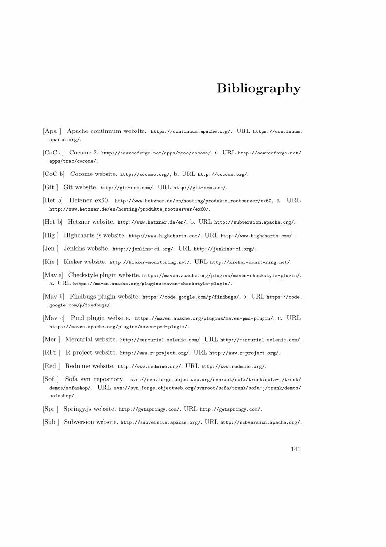
Bibliography
[Apa ] Apache continuum website. https://continuum.apache.org/. URL https://continuum.
apache.org/.
[CoC a] Cocome 2. http://sourceforge.net/apps/trac/cocome/, a. URL http://sourceforge.net/
apps/trac/cocome/.
[CoC b] Cocome website. http://cocome.org/, b. URL http://cocome.org/.
[Git ] Git website. http://git-scm.com/. URL http://git-scm.com/.
[Het a] Hetzner ex60. http://www.hetzner.de/en/hosting/produkte_rootserver/ex60, a. URLhttp://www.hetzner.de/en/hosting/produkte_rootserver/ex60/.
[Het b] Hetzner website. http://www.hetzner.de/en/, b. URL http://subversion.apache.org/.
[Hig ] Highcharts js website. http://www.highcharts.com/. URL http://www.highcharts.com/.
[Jen ] Jenkins website. http://jenkins-ci.org/. URL http://jenkins-ci.org/.
[Kie ] Kieker website. http://kieker-monitoring.net/. URL http://kieker-monitoring.net/.
[Mav a] Checkstyle plugin website. https://maven.apache.org/plugins/maven-checkstyle-plugin/,a. URL https://maven.apache.org/plugins/maven-checkstyle-plugin/.
[Mav b] Findbugs plugin website. https://code.google.com/p/findbugs/, b. URL https://code.
google.com/p/findbugs/.
[Mav c] Pmd plugin website. https://maven.apache.org/plugins/maven-pmd-plugin/, c. URLhttps://maven.apache.org/plugins/maven-pmd-plugin/.
[Mer ] Mercurial website. http://mercurial.selenic.com/. URL http://mercurial.selenic.com/.
[RPr ] R project website. http://www.r-project.org/. URL http://www.r-project.org/.
[Red ] Redmine website. http://www.redmine.org/. URL http://www.redmine.org/.
[Sof ] Sofa svn repository. svn://svn.forge.objectweb.org/svnroot/sofa/trunk/sofa-j/trunk/
demos/sofashop/. URL svn://svn.forge.objectweb.org/svnroot/sofa/trunk/sofa-j/trunk/demos/
sofashop/.
[Spr ] Springy.js website. http://getspringy.com/. URL http://getspringy.com/.
[Sub ] Subversion website. http://subversion.apache.org/. URL http://subversion.apache.org/.
141
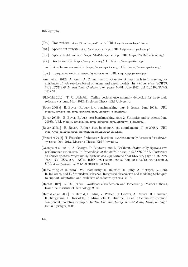
Bibliography
[Tra ] Trac website. http://trac.edgewall.org/. URL http://trac.edgewall.org/.
[ant ] Apache ant website. http://ant.apache.org/. URL http://ant.apache.org/.
[bui ] Apache buildr website. https://buildr.apache.org/. URL https://buildr.apache.org/.
[gra ] Gradle website. http://www.gradle.org/. URL http://www.gradle.org/.
[mav ] Apache maven website. http://maven.apache.org/. URL http://maven.apache.org/.
[mys ] mysqltuner website. http://mysqltuner.pl. URL http://mysqltuner.pl/.
[Amin et al. 2012] A. Amin, A. Colman, and L. Grunske. An approach to forecasting qosattributes of web services based on arima and garch models. In Web Services (ICWS),2012 IEEE 19th International Conference on, pages 74–81, June 2012. doi: 10.1109/ICWS.2012.37.
[Bielefeld 2012] T. C. Bielefeld. Online performance anomaly detection for large-scalesoftware systems, Mar. 2012. Diploma Thesis, Kiel University.
[Boyer 2008a] B. Boyer. Robust java benchmarking, part 1: Issues, June 2008a. URLhttps://www.ibm.com/developerworks/java/library/j-benchmark1/.
[Boyer 2008b] B. Boyer. Robust java benchmarking, part 2: Statistics and solutions, June2008b. URL https://www.ibm.com/developerworks/java/library/j-benchmark2/.
[Boyer 2008c] B. Boyer. Robust java benchmarking, supplements, June 2008c. URLhttp://www.ellipticgroup.com/html/benchmarkingArticle.html.
[Frotscher 2013] T. Frotscher. Architecture-based multivariate anomaly detection for softwaresystems, Oct. 2013. Master’s Thesis, Kiel University.
[Georges et al. 2007] A. Georges, D. Buytaert, and L. Eeckhout. Statistically rigorous javaperformance evaluation. In Proceedings of the 22Nd Annual ACM SIGPLAN Conferenceon Object-oriented Programming Systems and Applications, OOPSLA ’07, page 57–76, NewYork, NY, USA, 2007. ACM. ISBN 978-1-59593-786-5. doi: 10.1145/1297027.1297033.URL http://doi.acm.org/10.1145/1297027.1297033.
[Hasselbring et al. 2013] W. Hasselbring, R. Heinrich, R. Jung, A. Metzger, K. Pohl,R. Reussner, and E. Schmieders. iobserve: Integrated observation and modeling techniquesto support adaptation and evolution of software systems. 2013.
[Herbst 2012] N. R. Herbst. Workload classification and forecasting. Master’s thesis,Karsruhe Institute of Technology, 2012.
[Herold et al. 2008] S. Herold, H. Klus, Y. Welsch, C. Deiters, A. Rausch, R. Reussner,K. Krogmann, H. Koziolek, R. Mirandola, B. Hummel, et al. Cocome-the commoncomponent modeling example. In The Common Component Modeling Example, pages16–53. Springer, 2008.
142
Bibliography
[Jung et al. 2013] R. Jung, R. Heinrich, and E. Schmieders. Model-driven instrumentationwith kieker and palladio to forecast dynamic applications. In Symposium on SoftwarePerformance: Joint Kieker/Palladio Days 2013, volume 1083, pages 99–108. CEUR, 2013.
[Marwede et al. 2009] N. S. Marwede, M. Rohr, A. van Hoorn, and W. Hasselbring.Automatic failure diagnosis in distributed large-scale software systems based on timingbehavior anomaly correlation. In A. Winter, R. Ferenc, and J. Knodel, editors, Proceedingsof the 13th European Conference on Software Maintenance and Reengineering (CSMR’09),pages 47–57. IEEE, Mar. 2009. ISBN 978-0-7695-3589-0. doi: 10.1109/CSMR.2009.15.
[Project 2013] K. Project. Kieker user guide. Forschungsbericht, April 2013. URL http:
//eprints.uni-kiel.de/16537/.
[Salfner et al. 2010] F. Salfner, M. Lenk, and M. Malek. A survey of online failure predictionmethods. ACM Comput. Surv., 42(3):10:1–10:42, Mar. 2010. ISSN 0360-0300. doi:10.1145/1670679.1670680. URL http://doi.acm.org/10.1145/1670679.1670680.
[Shields 2010] G. Shields. The definitive guide to application performance management.International Journal on Advances in Software, 2010. URL https://www.gartner.com/doc/
2639025/magic-quadrant-application-performance-monitoring.
[van Hoorn ] A. van Hoorn. Dissertation - unpublished.
143