ONLINE APPENDIX for “Bargaining with Grandma: The Impact

ONLINE APPENDIX

for

“Bargaining with Grandma: The Impact of the South African Pension on Household Decision Making”

By: Kate Ambler, IFPRI

Appendix A: Comparison of NIDS Waves 1, 2, and 3

NIDS is a panel study that revisits participants every two to three years. At this time, the

first three waves of the NIDS data are publicly available; however this paper principally uses the

Wave 1 data due to a change in data collection protocol between Wave 1 and Waves 2 and 3.

Although the questions used to derive the main decision making variables used in the paper are

identical in all three waves, the changes in protocol affect the comparability of these variables. In

Wave 1, the survey protocol called for the household survey to be administered to the resident

household head. In Waves 2 and 3, surveyors were instructed to interview the oldest female in

the household. This change in protocol led to a much higher percent of older women being listed

as household head in Waves 2 and 3 compared to Wave 1. While this could have been due both

to surveyors being more likely to list the interviewee as the household head and to the

interviewee being more likely to identify herself as the household head, it seems likely that the

method employed in Wave 1 more likely led to the identification of the true head.

There are several ways to illustrate this change, but as an example, in Appendix Table 4,

I show the percentages of women aged 50 to 55 (who therefore would not have experienced a

change in pension status between Waves 1 and 3) who are identified as the household head in

Wave 1, Wave 2, and Wave 3. This is shown overall and by whether or not the woman lived with

an elderly male. The percentage of women identified as the household head jumps significantly

after Wave 1, from 53 percent to 61 percent and 59 percent in Waves 2 and 3 respectively). This

is particularly pronounced in households with an elderly male, where the percentage increases

from 15 to 29 in Wave 2 and 36 in Wave 3.

This household head variable is highly correlated with the decision making variables in

all waves. This is to be expected because characteristics of the household head are similar to the

1

characteristics of the decision maker. However, the correlation is also likely partly due to

measurement error in the decision making variables that occurs when surveyors or respondents

simply indicate the first name on the roster (the household head). Consequently, there is a similar

pattern between Wave 1 and Waves 2 and 3 in the decision making variables: women are much

more likely to be named the decision maker in Waves 2 and 3, compared to Wave 1. For

example, 31 percent of women aged 50 to 55 living with older men are the decision makers for

day to day purchases in Wave 1 and that figure jumps to 42 and 45 percent in Waves 2 and 3.

Because only two years pass between each wave, it is unlikely that this increase is due to actual

changes, but rather to the change in survey protocols.

It seems clear that Wave 1 contains the more accurate data for the analyses to be

conducted in this paper. Unfortunately, these large increases in percentages of non-pension

eligible elderly women who are reported to be the household head and the decision maker in

Waves 2 and 3 are such that the patterns found with the regression discontinuity analysis in

Wave 1 are not robustly apparent in Waves 2 and 3 (results shown and discussed in the main

text).1 However, the analysis presented here makes a strong argument that the inconsistency in

results is an artifact of the changes in the survey. Additionally, the income share analysis

presented in Section V is consistent across the three waves.2 Income share is a more objectively

1 The household head variable in Wave 1 exhibits a similar pattern to the decision making

variables: increases with female pension eligibility at age 60.

2 The correlation between decision making and income share is also twice as strong in Wave 1 as

it is in Waves 2 and 3, further supporting the argument that decision making is more accurately

measured in Wave 1.

2

measured variable than the decision making variables, and its consistency across the three

surveys is strong evidence the pension does result in a robust increase in women’s bargaining

power.

3

Appendix B: Household Outcomes

The analysis presenting in this paper of how pension eligibility affects decision making

and income share in the household is interesting in part because we expect these changes to

translate into changes in measures of well-being in the household. Although early impacts of the

pension have been extensively documented, it is important to document that they still exist in 2008,

15 years after the expansion of benefits. Here I examine impacts on child nutrition and ownership

of consumer durables, measures that are associated with the main decision-making categories that

I have addressed in this paper, decisions about day-to-day purchases such as groceries and about

large, unusual purchases such as many consumer durables.

A. Child nutrition

One of the most well-known results in the pension literature is Duflo’s finding that female

pension eligibility results in higher values of anthropometric indicators, including weight for

height, for young girls but not boys (Duflo, 2003). Weight for height is a flow measure of nutrition,

a marker that responds quickly when a child’s conditions changes. 1 In her main results using data

collected in 1993, Duflo finds a 0.61 standard deviation increase in the weight for height measure

for young girls with the presence of a pension eligible woman but a small and insignificant effect

with the presence of a pension eligible man. There are no statistically significant impacts for boys.

The NIDS survey collects anthropometric data from children, allowing for the construction

1 Weight for height Z-scores are calculated by subtracting the median and dividing by the

standard error for the child’s height and sex in a standard reference population. Duflo uses the

reference group of well-nourished US children provided by the U.S. National Center for Health

Statistics, standard prior to 2006.

4

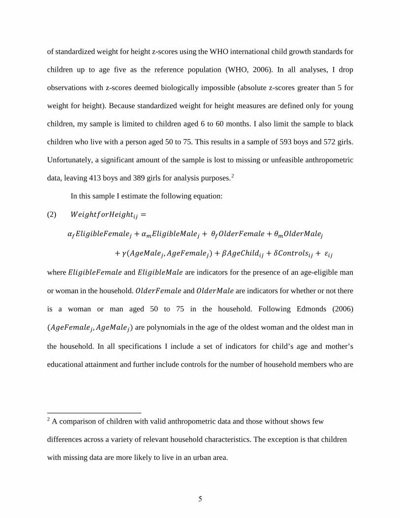
of standardized weight for height z-scores using the WHO international child growth standards for

children up to age five as the reference population (WHO, 2006). In all analyses, I drop

observations with z-scores deemed biologically impossible (absolute z-scores greater than 5 for

weight for height). Because standardized weight for height measures are defined only for young

children, my sample is limited to children aged 6 to 60 months. I also limit the sample to black

children who live with a person aged 50 to 75. This results in a sample of 593 boys and 572 girls.

Unfortunately, a significant amount of the sample is lost to missing or unfeasible anthropometric

data, leaving 413 boys and 389 girls for analysis purposes.2

In this sample I estimate the following equation:

(2) 𝑊𝑊𝑊𝑊𝑊𝑊𝑊𝑊ℎ𝑡𝑡𝑡𝑡𝑡𝑡𝑡𝑡𝑡𝑡𝑊𝑊𝑊𝑊𝑊𝑊ℎ𝑡𝑡𝑖𝑖𝑖𝑖 =

𝛼𝛼𝑓𝑓𝐸𝐸𝐸𝐸𝑊𝑊𝑊𝑊𝑊𝑊𝐸𝐸𝐸𝐸𝑊𝑊𝐸𝐸𝑊𝑊𝐸𝐸𝐸𝐸𝐸𝐸𝑊𝑊𝑖𝑖 + 𝛼𝛼𝑚𝑚𝐸𝐸𝐸𝐸𝑊𝑊𝑊𝑊𝑊𝑊𝐸𝐸𝐸𝐸𝑊𝑊𝐸𝐸𝐸𝐸𝐸𝐸𝑊𝑊𝑖𝑖 + 𝜃𝜃𝑓𝑓𝑂𝑂𝐸𝐸𝑂𝑂𝑊𝑊𝑡𝑡𝐸𝐸𝑊𝑊𝐸𝐸𝐸𝐸𝐸𝐸𝑊𝑊 + 𝜃𝜃𝑚𝑚𝑂𝑂𝐸𝐸𝑂𝑂𝑊𝑊𝑡𝑡𝐸𝐸𝐸𝐸𝐸𝐸𝑊𝑊𝑖𝑖

+ 𝛾𝛾(𝐴𝐴𝑊𝑊𝑊𝑊𝐸𝐸𝐸𝐸𝐸𝐸𝑊𝑊𝑖𝑖,𝐴𝐴𝑊𝑊𝑊𝑊𝐸𝐸𝑊𝑊𝐸𝐸𝐸𝐸𝐸𝐸𝑊𝑊𝑖𝑖) + 𝛽𝛽𝐴𝐴𝑊𝑊𝑊𝑊𝐴𝐴ℎ𝑊𝑊𝐸𝐸𝑂𝑂𝑖𝑖𝑖𝑖 + 𝛿𝛿𝐴𝐴𝑡𝑡𝐶𝐶𝑡𝑡𝑡𝑡𝑡𝑡𝐸𝐸𝐶𝐶𝑖𝑖𝑖𝑖 + 𝜀𝜀𝑖𝑖𝑖𝑖

where 𝐸𝐸𝐸𝐸𝑊𝑊𝑊𝑊𝑊𝑊𝐸𝐸𝐸𝐸𝑊𝑊𝐸𝐸𝑊𝑊𝐸𝐸𝐸𝐸𝐸𝐸𝑊𝑊 and 𝐸𝐸𝐸𝐸𝑊𝑊𝑊𝑊𝑊𝑊𝐸𝐸𝐸𝐸𝑊𝑊𝐸𝐸𝐸𝐸𝐸𝐸𝑊𝑊 are indicators for the presence of an age-eligible man

or woman in the household. 𝑂𝑂𝐸𝐸𝑂𝑂𝑊𝑊𝑡𝑡𝐸𝐸𝑊𝑊𝐸𝐸𝐸𝐸𝐸𝐸𝑊𝑊 and 𝑂𝑂𝐸𝐸𝑂𝑂𝑊𝑊𝑡𝑡𝐸𝐸𝐸𝐸𝐸𝐸𝑊𝑊 are indicators for whether or not there

is a woman or man aged 50 to 75 in the household. Following Edmonds (2006)

(𝐴𝐴𝑊𝑊𝑊𝑊𝐸𝐸𝑊𝑊𝐸𝐸𝐸𝐸𝐸𝐸𝑊𝑊𝑖𝑖,𝐴𝐴𝑊𝑊𝑊𝑊𝐸𝐸𝐸𝐸𝐸𝐸𝑊𝑊𝑖𝑖) are polynomials in the age of the oldest woman and the oldest man in

the household. In all specifications I include a set of indicators for child’s age and mother’s

educational attainment and further include controls for the number of household members who are

2 A comparison of children with valid anthropometric data and those without shows few

differences across a variety of relevant household characteristics. The exception is that children

with missing data are more likely to live in an urban area.

5

0-5, 6-14, 15-24, and 25-49, and the presence of mother and father in the household. 3 𝛼𝛼𝑓𝑓 and 𝛼𝛼𝑚𝑚

can then be interpreted as the difference in weight for height between a child living with a pension

eligible woman (man) and a child living with a woman (man) who is almost eligible. This

specification is similar to those used to estimate the impacts on decision making, but because the

level of observation is the child, not the older adult, it controls for age trends in the age of the

oldest man and woman in the household.

Appendix Table 7 shows the results of estimating this equation with girls in Panel 1 and

boys in Panel 2. Columns 1, 2, and 3 include linear, quadratic, and cubic age polynomials

respectively. Column 4 adds control variables to the cubic specification. The coefficient on woman

eligible is large and relatively stable across specifications for girls. The presence of a pension

eligible woman increases weight for height of girls by about 0.5 standard deviations. However the

effect is only statistically significant in the linear and quadratic specifications and only at the 10%

level. The coefficients for eligible man are small and have large standard errors, however I lack

the power to reject that the male and female coefficients are equal. In the boys sample all

coefficients are imprecisely estimated, although it should be noted that the coefficients for eligible

woman are positive. The pattern that emerges from these results is similar to the main results

reported by Duflo (2003). The presence of a pension eligible woman (but not a pension eligible

man) increases the weight for height of girls. There is no detectable effect of pension eligibility of

either gender for boys. However, given the selected sample, small sample size, and borderline

statistical significance of the results, they should not be over interpreted.

3 I do not include controls for father’s educational attainment because of the large number of

missing values.

6

B. Ownership of consumer durables

The significant increase in income provided by the pension provides the opportunity not

only to improve the quality of day-to-day purchases on food, but also to invest in larger household

items that have the ability to improve quality of life. The NIDS survey collects information on 27

separate durable goods that may be owned by households. Here I consider the total number of what

I term “household” durable goods, which are the 16 goods listed on the survey excluding

ownership of vehicles, bikes, and agricultural tools. The household durable goods include radios,

televisions, cell phones, appliances, and living room furniture.4 I observe only whether or not a

household possesses each type of good and do not know if they have more than one of each type.

Consequently, I can detect if pension eligible households buy types of goods that they did not

previously own, but not if they buy more of or replace goods that they already had.

I estimate the same household level model that I use in Section IV to examine changes in

decision making by other members of the household; the dependent variable is the number of

household durable goods. Appendix Table 8 presents the results. Panel 1 shows results for

households with an older woman aged 50 to 75 and Panel 2 for households with an older man.

Columns 1, 2, and 3 include linear, quadratic, and cubic age trends respectively and column 4 adds

control variables to the cubic specification.

4 The full list of included durable goods is: radio; Hi-Fi stereo; CD player; MP3 player;

television; satellite dish; VCR or DVD player; computer; camera; cell phone; electric stove; gas

stove; paraffin stove; microwave; fridge/freezer; washing machine; sewing/knitting machine;

lounge suite.

7

The results for households with an older woman are stable across specifications.

Focusing on columns 3 and 4, female eligibility results, on average, in ownership of 1.2 more

types of household durable goods, a 24% increase in the sample mean of 4.9. Women do appear

to be channeling some of their pension income into the purchase of consumer durables, a

complement to the fact that they were found to be significantly more likely to be the primary

decision maker for large, unusual purchases in the household. The coefficient on male eligibility

is marginally significant in the linear specification but is very sensitive to specification choice

and much smaller and insignificant in all other specifications. However, I cannot reject that the

coefficients on male and female eligibility are the same. Despite this, the evidence is overall

suggest that male pension eligibility does not lead to the purchase of more consumer durables.

8

Appendix C: Household Composition

As detailed in Section VII the main threat to the validity of the results in this paper is that

household reorganization associated with the pension eligibility of a household member is the true

driver of the observed results. Given the importance of this issue, in this appendix I provide

additional analyses to complement those in the main text.

Although the NIDS Wave 1 survey does not contain detailed information on non-resident

family members, I can use the data to perform several checks that will help understand whether

household reorganization is a threat to my results. First, NIDS collects information on remittances

sent to and from the household for or by anyone who is not a household resident. In fewer than

30% of households containing older men and women has anyone in the household sent or received

remittances in the past year, and this does not vary by pension eligibility (results not shown).

Although sending remittances is not a prerequisite for family decision making responsibilities to

be divided across non co-resident households, it is difficult to imagine the existence of a large

fraction of households where non-resident members dominate decision making for the entire

family but do not contribute economically to the family members with whom they are not living.

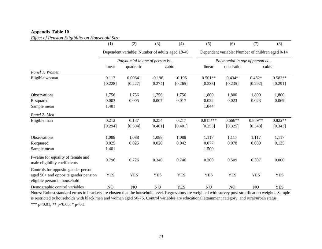
It is also possible to examine whether household composition changes with eligibility by

separately examining the number of prime age (18 to 49) adults and children (up to age 14) in the

household. The results are presented in Appendix Table 10. There is no evidence of any change in

the number of prime age adults (those whose departure could obfuscate the main results in the

paper) in households with older men or women. There is evidence of increases in the number of

children with both male and female eligibility, but flexibly controlling for the number of children

(or adults) in the household does not affect the female decision making results.

While persuasive, these results related to household size are not conclusive because they

9

could be masking changes in the types of the adults that live with pensioners, even if there is no

change in the overall number of adults. As noted in the main text, one of the benefits of the NIDS

survey is that because it is a panel study, individuals are tracked from wave to wave. I can use the

second wave of the survey to analyze changes from Wave 1 to Wave 2, under the assumption that

household reorganization patterns for individuals who are pension eligible in Wave 1 are similar

to the patterns for those are eligible in Wave 2. Using the sample of older adults aged 50 to 75 in

Wave 2, I identify those who left the older adults’ households between waves. First, I show that

those who were pension eligible in Wave 2 were not more likely to have had a household member

leave between waves (Appendix Table 11, columns 1 to 3). Additionally, because one of the

principal concerns in my analysis is whether the departure of likely candidates for decision making

led to a reduction in disagreement over the identity of the decision maker, I can specifically address

whether pension eligibility in Wave 2 is associated with those that left the pensioner’s household

between Wave 1 and Wave 2 being more likely to have been named by someone as the decision

maker in Wave 1.

I construct a variable for each person in Wave 1 that is equal to one if anyone in the

household named them as the decision maker for day to day purchases and zero otherwise. I then

identify, for each older adult in Wave 2, which individuals left their household between waves,

and take the average of the decision making variable just described for each older person across

individuals that left the household. I then test whether this variable differs with pension eligibility.

In other words, were those who left households with a person who was pension eligible more likely

to have been named by someone as the decision maker in Wave 1 than those who left households

with a person who was not pension eligible? The results are presented in Appendix Table 11

(columns 4 to 6). In short, there is no evidence that the decision making power of leavers varies

10

with eligibility, making it unlikely that this is what could have driven increases in female decision

making power in Wave 1.

11

Appendix D: Appendix Figures and Tables

12

Appendix Figure 1: Number of Observations per Age

Appendix Figure 2: Primary Decision Making for Day to Day Purchases by Age, Two Year Age Bins

Appendix Figure 3: Personal Income Share of Oldest Male by Age

Notes: Sample is individuals aged 50 to 75. Appendix Figure 1: Scatterplot is number of observations per age. Appendix Figures 2 & 3: Scatterplots are unweighted means of y-axis variable by age in years. Unweighted OLS regression lines of y-axis variable on age are estimated on either side of the discontinuity. 95% confidence intervals are shown around the regression lines. Y-axis variables are dummy variable for whether or not everyone in household agrees that individual is the primary decision maker for where household lives (Appendix Figure 2) and personal income share of oldest male in household (Appendix Figure 3). In Appendix Figure 3 the top half percent of male and female household income earners are trimmed and sample is limited to women 50 to 75 living with an older male.

2040

6080

100

120

Num

ber o

f obs

erva

tions

50 55 60 65 70 75Age

Panel A: Women

2040

6080

100

120

Num

ber o

f obs

erva

tions

50 55 60 65 70 75Age

Panel B: Men.4

.5.6

.7.8

Mea

n of

dec

ision

mak

ing

50 55 60 65 70 75Age

Panel A: Women

.4.5

.6.7

.8M

ean

of d

ecisi

on m

akin

g

50 55 60 65 70 75Age

Panel B: Men

2030

4050

Mea

n pe

rcen

t of h

h in

com

e - m

en

50 55 60 65 70 75Age of woman

Women living with a man 50+

13

(1) (2) (3) (4)

linear quadraticPanel 1: WomenPension eligible 0.620*** 0.625*** 0.572*** 0.578***

[0.0454] [0.0445] [0.0653] [0.0635]

Observations 1,763 1,763 1,763 1,763R-squared 0.668 0.668 0.670 0.674Sample mean 0.484

Panel 2: MenPension eligible 0.485*** 0.361*** 0.328*** 0.339***

[0.0650] [0.0836] [0.0915] [0.0888]


Controls for opposite gender person aged 50+ and opposite gender pension eligible person in household

YES YES YES YES

Demographic control variables NO NO NO YES

*** p<0.01, ** p<0.05, * p<0.1

Appendix Table 1

Dependent variable: Pension receiptPolynomial in age of person is…

cubic

P-value for equality of female and male eligibility coefficients 0.093 0.005 0.031 0.028

Effect of Pension Eligibility on Pension Receipt

Notes: Robust standard errors in brackets are clustered at the household level. Regressions are weighted with survey post-stratification weights. Sample is restricted to black men and women aged 50-75. Control variables are number of household members who are 0-5, 6-14, 15-24, and 25-49, educational attainment category, and rural/urban status.

14

(1) (2) (3) (4) (5) (6) (7) (8) (9) (10) (11) (12)

linear quadratic linear quadratic linear quadraticPanel 1: WomenPension eligible 0.121*** 0.133*** 0.154** 0.137** 0.126*** 0.137*** 0.174*** 0.159*** 0.123*** 0.133*** 0.148*** 0.132***

[0.0462] [0.0485] [0.0603] [0.0590] [0.0400] [0.0423] [0.0500] [0.0498] [0.0401] [0.0435] [0.0499] [0.0499]Presence of man 50+ -0.627*** -0.628*** -0.629*** -0.627*** -0.671*** -0.671*** -0.672*** -0.673*** -0.648*** -0.649*** -0.649*** -0.649***

[0.0318] [0.0317] [0.0319] [0.0329] [0.0287] [0.0287] [0.0287] [0.0289] [0.0304] [0.0305] [0.0305] [0.0310]-0.0165 -0.0125 -0.0117 -0.00550 -0.0472 -0.0437 -0.0419 -0.0274 -0.0796** -0.0765** -0.0759** -0.0617[0.0453] [0.0453] [0.0456] [0.0466] [0.0371] [0.0372] [0.0375] [0.0382] [0.0369] [0.0373] [0.0375] [0.0387]

Observations 1,769 1,769 1,769 1,769 1,787 1,787 1,787 1,787 1,787 1,787 1,787 1,787R-squared 0.369 0.370 0.370 0.379 0.435 0.435 0.436 0.450 0.426 0.427 0.427 0.441Sample mean 0.641 0.641 0.600

Panel 2: MenPension eligible -0.0456 -0.0676 -0.145 -0.117 -0.129* -0.157* -0.258*** -0.249*** -0.114 -0.0991 -0.183* -0.161*

[0.0803] [0.0997] [0.108] [0.0959] [0.0742] [0.0908] [0.0999] [0.0890] [0.0756] [0.0939] [0.103] [0.0899]Presence of woman 50+ -0.158*** -0.156*** -0.153*** -0.127*** -0.0898** -0.0872** -0.0835* -0.0746* -0.119*** -0.120*** -0.117*** -0.104**

[0.0469] [0.0471] [0.0470] [0.0455] [0.0442] [0.0443] [0.0443] [0.0448] [0.0449] [0.0450] [0.0449] [0.0444]-0.0482 -0.0505 -0.0595 -0.0388 -0.0769 -0.0801 -0.0907 -0.0652 -0.0697 -0.0679 -0.0768 -0.0554[0.0604] [0.0606] [0.0601] [0.0587] [0.0577] [0.0584] [0.0576] [0.0572] [0.0585] [0.0591] [0.0585] [0.0579]

Observations 1,094 1,094 1,094 1,094 1,106 1,106 1,106 1,106 1,106 1,106 1,106 1,106R-squared 0.030 0.030 0.034 0.131 0.021 0.021 0.027 0.125 0.026 0.026 0.030 0.128Sample mean 0.646 0.699 0.693

Control variables NO NO NO YES NO NO NO YES NO NO NO YES

*** p<0.01, ** p<0.05, * p<0.1

Dependent variable: Primary decision maker for who can live in household

cubic


P-value for equality of female and male eligibility coefficients

0.067 0.061 0.013 0.021

Presence of pension eligible man

Presence of pension eligible woman

0.004 0.0050.002 0.003 0.000 0.000 0.004 0.025

Appendix Table 2

Polynomial in age of person is…

Dependent variable: Primary decision maker for large, unusual purchases

Dependent variable: Primary decision maker for where household lives

cubic cubic

Effect of Pension Eligibility on Household Decision Making: Other Decision Making Categories

15

(1) (2) (3) (4) (5) (6) (7) (8)

linear quadratic linear quadraticPanel 1: WomenPension eligible 0.156*** 0.120 0.170 0.129 0.143*** 0.159** 0.146 0.112

[0.0474] [0.0777] [0.121] [0.118] [0.0448] [0.0747] [0.125] [0.123]Presence of man 50+ -0.555*** -0.555*** -0.554*** -0.562*** -0.656*** -0.657*** -0.656*** -0.655***

[0.0357] [0.0357] [0.0357] [0.0348] [0.0282] [0.0283] [0.0283] [0.0288]-0.055 -0.055 -0.057 -0.037 -0.0318 -0.0302 -0.0308 -0.0133

[0.0497] [0.0503] [0.0502] [0.0497] [0.0346] [0.0352] [0.0352] [0.0363]

Observations 1,794 1,794 1,794 1,794 1,764 1,764 1,764 1,764R-squared 0.321 0.321 0.323 0.347 0.401 0.402 0.403 0.420Sample mean 0.642 0.572

Panel 2: MenPension eligible -0.044 -0.129 -0.094 -0.078 -0.0570 -0.204 -0.178 -0.156

[0.0879] [0.128] [0.180] [0.160] [0.0898] [0.129] [0.178] [0.160]Presence of woman 50+ -0.236*** -0.233*** -0.233*** -0.203*** -0.238*** -0.235*** -0.235*** -0.217***

[0.0470] [0.0473] [0.0472] [0.0452] [0.0474] [0.0476] [0.0476] [0.0453]-0.047 -0.053 -0.049 -0.029 -0.0538 -0.0601 -0.0584 -0.0320

[0.0585] [0.0590] [0.0589] [0.0576] [0.0580] [0.0584] [0.0584] [0.0569]


Control variables NO NO NO YES NO NO NO YESNotes: Robust standard errors in brackets are clustered at the household level. Regressions are weighted with survey post-stratification weights. Sample is restricted to black men and women aged 50-75. Control variables are number of household members who are 0-5, 6-14, 15-24, and 25-49, educational attainment category, and rural/urban status.

*** p<0.01, ** p<0.05, * p<0.1

Appendix Table 3

Dependent variable: Primary decision maker for day-to-day purchases

Dependent variable: Primary decision maker for all categories

Polynomial in age of person is…cubic cubic

Effect of Pension Eligibility on Household Decision Making: Flexible Polynomials

Presence of pension eligible man

Presence of pension eligible woman

16

All No man 50+ in hh Man 50+ in hh

Household headWave 1 53.1 79.6 15.3Wave 2 60.7 83.0 29.1Wave 3 59.3 74.6 35.8

Primary decision maker for day to day purchasesWave 1 60.1 80.6 30.8Wave 2 63.3 78.2 42.0Wave 3 64.6 77.7 44.7

Notes: Author's calculations from NIDS Waves 1, 2, and 3.

Appendix Table 4

Women 50 - 55Comparison of NIDS Wave 1, Wave 2, and Wave 3

17

(1) (2) (3) (4) (5) (6) (7) (8)

linear quadratic linear quadraticPanel 1: WomenPension eligible 14.58*** 16.35*** 18.54*** 16.21*** -5.709*** -4.320* -3.616 -5.454**

[3.330] [3.605] [4.181] [3.724] [2.077] [2.595] [2.718] [2.713]


Panel 2: MenPension eligible -1.422 -1.274 -3.773 -0.411 -13.07** -12.30*** -9.671 -6.931

[5.367] [5.078] [7.120] [6.470] [5.530] [4.588] [7.072] [6.688]



YES YES YES YES YES YES YES YES

Demographic control variables NO NO NO YES NO NO NO YES

Appendix Table 5Effect of Pension Eligibility on Income Variables

Dependent variable: Personal income share

Polynomial in age of person is…cubic

Dependent variable: Labor income as percent of household non-pension income

Polynomial in age of person is…cubic

*** p<0.01, ** p<0.05, * p<0.1



0.217 0.135 0.429 0.839

18

(1) (2) (3) (4) (5) (6) (7) (8)

linear quadratic linear quadraticPanel 1: WomenPension eligible 316.9 425.6 239.3 164.2 0.215** 0.238** 0.172 0.149

[372.8] [424.9] [494.7] [419.6] [0.0947] [0.107] [0.119] [0.0988]

Observations 1,746 1,746 1,746 1,746 1,746 1,746 1,746 1,746R-squared 0.039 0.040 0.040 0.313 0.052 0.053 0.053 0.368Sample mean 2731

Panel 2: MenPension eligible 742.4 764.5 1,538 1,852* 0.264 0.206 0.368 0.423**

[957.7] [1,239] [1,361] [963.8] [0.170] [0.187] [0.239] [0.181]

Observations 1,082 1,082 1,082 1,082 1,082 1,082 1,082 1,082R-squared 0.004 0.004 0.007 0.323 0.027 0.028 0.031 0.361Sample mean 3231




Appendix Table 6

0.883 0.457 0.189


0.802

cubic cubic

Effect of Pension Eligibility on Household Income

Dependent variable: Household income Dependent variable: Log household income

Polynomial in age of person is… Polynomial in age of person is…


*** p<0.01, ** p<0.05, * p<0.1

19

(1) (2) (3) (4)

linear quadratic

Panel 1: GirlsEligible woman 0.480* 0.482* 0.478 0.400

[0.290] [0.280] [0.340] [0.324]Eligible man 0.025 0.250 0.203 0.104

[0.296] [0.391] [0.395] [0.398]

P-value for equality of eligible woman and eligible man 0.221 0.154 0.245 0.393

Observations 399 399 399 399R-squared 0.086 0.090 0.104 0.150

Panel 2: BoysEligible woman 0.332 0.358 0.247 0.179

[0.291] [0.293] [0.350] [0.350]Eligible man -0.188 -0.113 -0.347 -0.305

[0.295] [0.423] [0.426] [0.446]

P-value for equality of eligible woman and eligible man 0.450 0.463 0.647 0.755

Observations 413 413 413 413R-squared 0.052 0.053 0.062 0.090

Control variables NO NO NO YES

Effect of Pension Eligibility on Weight for Height Z-scores

*** p<0.01, ** p<0.05, * p<0.1

Appendix Table 7

Polynomial in age of oldest man and oldest woman is…

cubic

Notes: Robust standard errors in brackets are clustered at the household level. Regressions are weighted with survey post-stratification weights. Sample is restricted to black boys and girls aged 6 to 60 months who live with a person aged 50-75 and have non-missing, valid anthropometric data. All regressions control for age of child. Control variables are number of household members who are 0-5, 6-14, 15-24, and 25-49, mother's educational attainment category, and presence of mother and father in the household.

20

(1) (2) (3) (4)

linear quadratic

Eligible woman 0.946** 1.175*** 1.213*** 1.202***[0.392] [0.421] [0.437] [0.432]

Presence of man 50+ 0.673** 0.655** 0.654** 0.578*[0.328] [0.330] [0.329] [0.296]

Eligible man -0.106 -0.039 -0.037 0.299[0.453] [0.459] [0.459] [0.394]


Eligible man 1.168* 0.587 0.413 0.705[0.639] [0.700] [0.796] [0.698]

Presence of woman 50+ 1.273*** 1.329*** 1.336*** 1.525***[0.383] [0.383] [0.383] [0.336]

Eligible woman 0.099 0.026 0.007 -0.204[0.434] [0.446] [0.443] [0.383]


Control variables NO NO NO YES

*** p<0.01, ** p<0.05, * p<0.1

Appendix Table 8

cubic

Panel 2: Households with a man 50 - 75

Panel 1: Households with a woman 50 - 75

Polynomial in age of oldest man or oldest woman is…


Effect of Pension Eligibility on Number of Household Consumer Durables

Notes: Robust standard errors in brackets are clustered at the survey cluster level. Regressions are weighted with survey post-stratification weights. Sample is restricted to households with a black woman (man) aged 50 -75. Control variables are number of household members who are 0-5, 6-14, 15-24, and 25-49. Household durable goods include radio; Hi-Fi stereo, CD player, MP3 player; television; satellite dish; VCR or DVD player; computer; camera; cell phone; electric stove; gas stove; paraffin stove; microwave; fridge/freezer; washing machine; sewing/knitting machine; lounge suite.

21

Effect of Pension Eligiblity in 1993: PSLSD Data(1) (2) (3) (4) (5) (6)

linear quadratic cubic linear quadratic cubicPanel 1: WomenPension eligible 0.388*** 0.382*** 0.255*** 13.49*** 12.22*** 4.648

[0.0484] [0.0496] [0.0610] [3.617] [3.835] [4.524]

Observations 1,082 1,082 1,082 1,079 1,079 1,079R-squared 0.476 0.476 0.488 0.170 0.170 0.179Sample mean 0.476 32.40

Panel 2: MenPension eligible 0.206*** 0.142* 0.0562 7.141 6.313 4.307

[0.0626] [0.0754] [0.0824] [5.052] [5.458] [6.447]

Observations 764 764 764 763 763 763R-squared 0.354 0.360 0.365 0.048 0.048 0.049Sample mean 0.251 34.92


YES YES YES YES YES YES

Demographic control variables NO NO NO NO NO NO

*** p<0.01, ** p<0.05, * p<0.1

Appendix Table 9

Dependent variable: Pension receipt

Polynomial in age of person is… Polynomial in age of person is…

Dependent variable: Personal income share

Notes: Robust standard errors in brackets are clustered at the household level. Sample is restricted to black men and women aged 50-75 in households with a child 6 to 60 months.

P-value for equality of female and male eligibility coefficients 0.021 0.008 0.051 0.307 0.376 0.966

22

(1) (2) (3) (4) (5) (6) (7) (8)

linear quadratic linear quadraticPanel 1: WomenEligible woman 0.117 0.00641 -0.196 -0.195 0.501** 0.434* 0.482* 0.583**

[0.228] [0.227] [0.274] [0.265] [0.235] [0.235] [0.292] [0.291]


Panel 2: MenEligible man 0.212 0.137 0.254 0.217 0.815*** 0.666** 0.889** 0.822**

[0.294] [0.304] [0.401] [0.401] [0.253] [0.325] [0.348] [0.343]





Effect of Pension Eligibility on Household SizeAppendix Table 10

Dependent variable: Number of adults aged 18-49 Dependent variable: Number of children aged 0-14

Polynomial in age of person is… Polynomial in age of person is…cubic cubic

*** p<0.01, ** p<0.05, * p<0.1

Notes: Robust standard errors in brackets are clustered at the household level. Regressions are weighted with survey post-stratification weights. Sample is restricted to households with black men and women aged 50-75. Control variables are educational attainment category, and rural/urban status.

P-value for equality of female and male eligibility coefficients 0.796 0.726 0.340 0.746 0.300 0.509 0.307 0.000

23

(1) (2) (3) (4) (5) (6)

linear quadratic cubic linear quadratic cubicPanel 1: WomenWave 2 pension eligible -0.155 -0.157 -0.0900 -0.00678 -0.000102 0.0321

[0.137] [0.130] [0.158] [0.0773] [0.0761] [0.0994]

Observations 1,721 1,721 1,721 470 470 470R-squared 0.005 0.005 0.005 0.066 0.066 0.067Sample mean 0.442 0.162

Panel 2: MenWave 2 pension eligible 0.230 0.239 0.249 0.0257 -0.00278 0.0429

[0.150] [0.152] [0.194] [0.0802] [0.0792] [0.0800]

Observations 982 982 982 242 242 242R-squared 0.017 0.017 0.017 0.038 0.052 0.055Sample mean 0.398 0.109

Controls for opposite gender person aged 50+ and opposite gender pension eligible person in household in W2

YES YES YES YES YES YES

Pension Eligibility and Household Leavers

Dependent variable: Total number of those leaving household between W1

and W2

*** p<0.01, ** p<0.05, * p<0.1

Dependent variable: Average value of day-to-day decision making variable for

those leaving household between W1 and W2

Appendix Table 11

Polynomial in Wave 2 age of person is…

Notes: Robust standard errors in brackets are clustered at the household level. Regressions are weighted with survey post-stratification weights. Sample is restricted to black men and women aged 50-75 in NIDS Wave 2. Sample in columns 4 to 6 is additionally restricted to people who had someone leave their household between Wave 1 and Wave 2.

24

Documents

ONLINE APPENDIX for “Bargaining with Grandma: The Impact