Online Appendix Evidence from Malawi Dean Yang Appendix A ...econweb.umd.edu/~goldberg/docs/gine_goldberg_yang... · Background on Cheetah Paprika (CP) Extension services provided

Online Appendix for Credit Market Consequences of Improved Personal Identification: Field Experimental Evidence from Malawi Xavier Giné Jessica Goldberg Dean Yang Appendix A: Background on project partners, loan details, and full text of training script

Background on Cheetah Paprika (CP) Extension services provided by CP consist of preliminary meetings to market paprika

seed to farmers and teach them about the growing process, additional group trainings about farming techniques, individual support for growers provided by the field assistants, and information about grading and marketing the crop. The farmer receives extension services and a package of seeds, pesticides and fungicides at wholesale rates in exchange for the commitment to sell the paprika crop to CP at harvest time. Although CP is by far the largest paprika purchaser in the country, it does not provide credit to farmers because of the risks involved in contract enforcement.1 CP has a staff of six extension officers and 15 field assistants in the locations chosen for the study. The staff maintain a database of all current and past paprika growers and handles the logistics of supplying farmers with the package of inputs as well as the purchase of the crop.

In July 2007, CP asked farmers in the study areas to organize themselves into clubs of 15 to 20 members to accommodate MRFC’s group lending rules.2 Most of these clubs were already in existence, primarily to ease delivery of Cheetah extension services and collection of the crop. During the baseline survey and fingerprinting period (August and September 2007), CP staff provided a list of paprika growing clubs in each locality to be visited in each week.

Background on MRFC and loan details MRFC is a government-owned microfinance institution and is the largest provider of

rural finance, with a nationwide outreach of 210,000 borrowers in 2007. To obtain the loan-financed production inputs, borrowers took an authorization form from MRFC to a pre-approved agricultural input supplier who provided the inputs to the farmer and billed MRFC at a later date. Sixty percent of the loan went towards fertilizer (one 50 kilogram bag of D-compound fertilizer and two 50 kilogram bags of CAN fertilizer); the rest went toward the CP input package: thirty-three percent covered the cost of nine bags of pesticides and fungicides (2 Funguran, 2 Dithane, 2 Benomyl, 1 Cypermethrin, 1 Acephate and 1 Malathion) and the remaining seven percent for

1 In 2007, CP purchased approximately eighty-five percent of the one thousand tons of paprika produced annually in Malawi. 2 A typical CP group has between 15 and 30 farmers and is organized around a paprika collection point. MRFC’s lending groups have at most 20 farmers, so some of the CP groups participating in the study had to be split to be able to access MRFC’s loans.

Online appendix page 1

the purchase of 0.4 kilograms of seeds.3 While all farmers that took the loan were given the CP package, farmers had the option to borrow only one of the two available bags of CAN fertilizer. Expected yield for farmers using the package with two bags of CAN fertilizer on one acre of land was between 400 and 600 kg, compared to 200 kg with no inputs.4 In keeping with standard MRFC practices, farmers were expected to raise a 15 percent deposit, and were charged interest of 33 percent per year (or 30 percent for repeat borrowers). Biometric training script Benefits of Good Credit Having a record of paying back your loans can help you get bigger loans or better interest rates. Credit history works like trust. When you know someone for a long time, and that person is honest and fair when you deal with him, then you trust him. You are more likely to help him, and he is more likely to help you. You might let him use your hoe (or something else that is important to you), because you feel sure that he will give it back to you. Banks feel the same way about customers who have been honest and careful about paying back their loans. They trust those customers, and are more willing to let them borrow money. MRFC already gives customers who have been good borrowers a reward. It charges them a lower interest rate, 30 percent instead of 33 percent. That means that for the loan we have described today, someone who has a good credit history would only have to pay back 8855, instead of 8971.5 Another way that banks might reward customers they trust is by letting them borrow bigger amounts of money. Instead of 7700 MK to grow one acre of paprika, MRFC might lend a trusted customer 15400, to grow two acres. To earn trust with the bank, and get those rewards, you have to be able to prove to the bank that you have taken loans before and paid them back on time. You can do that by making sure that you give the bank accurate information when you fill out loan applications. But if you call yourself John Jacob Phiri one year, and Jacob John Phiri the next year, then the bank might not figure out that you are the same person, so they won’t give you the rewards you have earned. Costs of Bad Credit But trust can be broken. If your neighbor borrows your radio and does not give it back or it gets ruined, then you probably wouldn’t lend him anything else until the radio had been replaced. Banks work the same way. If you take a loan and break the trust between yourself and the bank by not paying back the loan, then the bank won’t lend to you again. This is especially true if you have a good harvest but still choose not to pay back the loan. When you apply for a loan, one of the things that a bank does to decide whether or not to accept your application is to look in its records to see if you have borrowed money before. If you have borrowed but not paid back, then you will be turned down for the new loan. This is like you asking your neighbors if someone new shows up in the village and asks you to work for him. You might first ask around to see if the person is fair to his employees and

3 The loan amount varied across locations because of modest differences in the transport cost for fertilizer. The cost of the CP package was the same in all locations. 4 Yield is computed under the conservative assumption that farmers will divert one 50 Kg bag of CAN fertilizer towards maize cultivation. While larger quantities of inputs would result in higher output for experienced paprika-growers, the package described here was designed by extension experts to maximize expected profits for novice, small-holder growers. 5 Loan amounts mentioned in the script are lower than actual loan amounts observed in the data because fertilizer prices rose somewhat in the time between the initial intervention (in Aug-Sep 2007) and loan disbursement (Nov 2007).


pays them on time. If you learn that the person does not pay his workers, then you won’t work for him. Banks do the same thing by checking their records. MRFC does not ever give new loans to people who still owe them money. And MRFC shares information about who owes money with other banks, so if you fail to pay back a loan from MRFC, it can stop you from getting a new loan from OIBM or another lender, also. Remainder of script is administered to fingerprinted clubs only Biometric Technology Fingerprints are unique, which means that no two people can ever have the same fingerprints. Even if they look similar on a piece of paper, people with special training, or special computer equipment, can always tell them apart. Your fingerprint can never change. It will be the same next year as it is this year. Just like the spots on a goat are the same as long as the goat lives, but different goats have different spots. Fingerprints can be collected with ink and paper, or they can be collected with special machines. This machine stores fingerprints in a computer. Once your fingerprint is stored in the computer, then the machine can recognize you, and know your name and which village you come from, just by your fingerprint! The machine will recognize you even if the person who is using it is someone you have never met before. The information from the machines is saved in many different ways, so if one machine breaks, the information is still there. Just like when Celtel’s building burned, people’s phone numbers did not change. Administer the following after all fingerprints have been collected: Demo Now, I can figure out your name even if you don’t tell me. Will someone volunteer to test me? (Have a volunteer swipe his finger, and then tell everyone who it was). The bank will store information about your loans with your fingerprint. That means that bank officers will know not just your name, but also what loans you have taken and whether or not you have paid them back. They will be able to tell all of this just by having you put your finger on the machine. Before, banks used your name and other information to find out about your credit history. But now they will use fingerprints to find out. This means that even if you tell the bank a different name, they will still be able to find all of your loan records. Names can change, but fingerprints cannot. Having your fingerprint on file can make it easier to earn the rewards for good credit history that we talked about earlier. It will be easy for the bank to look up your records and see that you have paid back your loans before. It will also be easier to apply for loans, because there will be no new forms to fill out in the future! But, having your fingerprint on file also makes the punishment for not paying back your loan much more certain. Even if you tell the bank a different name than you used before, or meet a different loan officer, or go to a different branch, the bank will just have to check your fingerprint to find out whether or not you paid your loans before. Having records of fingerprints also makes it easy for banks to share information. Banks will share information about your fingerprints and loans. If you don’t pay back a loan to MRFC, OIBM will know about it! Appendix B: Details on biometric fingerprinting technology

In consultation with MRFC’s management, fingerprint recognition was chosen over face, iris or retina recognition because it is the cheapest, best known and most widely used biometric identification technology. Fingerprinting technology extracts features from impressions made by the distinct ridges on the fingertips and has been commercially available since the early 1970s.


Loan applicants from fingerprinted clubs had the image of their right thumb fingerprint captured by an optical fingerprint scanner attached to a laptop. To maximize accuracy, farmers washed their thumbprints prior to scanning, and the scanner was also cleaned after each impression. During collection, about 2 per cent of farmers had the left thumbprint recorded (instead of the right) because the right thumbprint was worn out. (Many farmers grow tobacco, which involves thumb usage during seedling transplantation that can wear out a thumbprint over many years.)

Upon scanning, the fingerprint image was enhanced and added to the borrower database. We purchased the VeriFinger 5.0 Software Development Kit from Fulcrum Biometrics and had a programmer develop a data capture program that would allow the user to (i) enter basic demographic information such as the name, address, village, loan size and the unique BFIRM identifier, (ii) capture the fingerprint with the scanner and (iii) review the fingerprint alongside the demographic information. Appendix C: Variable definitions Data used in this paper come from two surveys: a baseline conducted in August-September 2007 and a follow-up survey about farm outputs and other outcomes conducted in August 2008. We also used administrative data about loan take-up and repayment, obtained from MRFC’s internal records. Baseline characteristics (from baseline survey) Male equals 1 for men and 0 for women. Married equals 1 for married respondents and 0 for respondents who are single, widowed, or divorced. Age is respondent’s age in years. In regressions, we use dummies for 5-year age categories rather than a continuous measure of age. Years of education is years of completed schooling, and is top-coded at 13. In regressions, we use dummies for years of completed schooling, rather than a continuous measure of education. Risk taker equals 1 for respondents who report that they frequently take risks, and 0 for respondents who do not. Days of hunger last year is the number of days in the 2006-2007 season that individuals reduced the number of meals they ate per day. Late paying previous loan equals 1 for respondents who report paying back a previous loan late, and 0 for respondents who do not. Income SD is the standard deviation of income between the self-reported best and worst incomes of the 5 most recent years. Years of experience growing paprika is the self reported number of seasons in which the respondent has grown paprika before the season studied in this project. Previous default equals 1 for respondents who report that they have defaulted on a previous loan and 0 otherwise. No previous loans equals 1 for respondents who report that they have not had any other loans from formal financial institutions (including micro lenders, savings and credit cooperatives, and NGO schemes) and 0 otherwise.


Take-up and repayment (from administrative data) Approved equals 1 if the respondent was approved by MRFC for a loan and 0 otherwise. Any loan equals 1 if the respondent borrowed money from MRFC and 0 otherwise (this could differ from Approved if the respondent chose not to take out the loan after it was approved by MRFC). Total borrowed is the amount owed to MRFC, in Malawi kwacha (MK 145 = $US 1). This includes the loan principal and 33 percent interest charged by MRFC. Balance is the unpaid loan amount remaining to be paid to MRFC. The balance includes principal and accumulated interest, and is reported in MK. Fraction paid is the amount paid on the loan, divided by the total borrowed defined above. Fully paid equals 1 if the respondent has completely repaid the loan and 0 if there is an outstanding balance. We examine different versions of the variables Balance, Fraction paid, and Fully paid that vary by the date at which loan repayment status is measured. One set of variables refers to loan repayment status as of September 30, 2008, which is the formal due date of the loan. Another set of variables refers to “eventual” repayment as of the end of November 2008. MRFC considers loan repayment status at the end of November 2008 as the final repayment status of the loan, and makes no subsequent attempts to collect loan repayments after that point. Land use and inputs (from follow-up survey) Fraction of land used for various crops is the land used for the given crop, divided by total land cultivated. Seeds is the value of paprika seeds used by the respondent, in MK. Fertilizer is the value of all chemical fertilizer used by the respondent on the paprika crop, in MK. Chemicals is the value of all pesticides and herbicides used by the respondent on the paprika crop, in MK. Man-days is the amount of money spent on hired, non-family labor for the paprika crop, in MK. All paid inputs is the total amount of money spent on inputs for the paprika crop, in MK. Mathematically, it is the sum of Seeds, Fertilizer, Chemicals, and Man-days defined above. KG manure is the kilograms of manure applied to the paprika crop. Times weeding is the number of times the paprika crop was weeded, by the respondent or hired labor. Output, revenue and profits (from follow-up survey) KG of various crops is the self-reported kilograms harvested of each crop. Market sales is the amount of MK received from any sales of maize, soya, groundnuts, tobacco, paprika, tomatoes, leafy vegetables, and cabbage between April and August, which encompasses the entire main harvest and selling season for these crops.


Profits is the value of Market sales, plus the value of unsold crop estimated based on the farmer’s reported quantity, valued at district average price reported by the EPA office (Value of unsold harvest, defined below), minus All paid inputs as defined above. Value of unsold harvest is the value, in MK, of the difference between the kg harvested and the kg sold of each crop. We use district average prices, as reported by the EPA office. Appendix D: The Model

By virtue of the experiment, the credit contract is kept fixed, so our goal here is not to solve for the optimal contract in the presence of both information asymmetries (Gesnerie, Picard and Rey, 1988 or Chassagnon and Chiappori, 1997 for risk averse agents), but rather to derive the agents’ optimal behavior with and without dynamic incentives.

Agents (or farmers) are risk-neutral and decide how much to borrow for cash crop inputs and how much to invest. We assume that they do not have collateral or liquid assets, so the maximum they can invest in cash crop production is the loan amount.

We introduce the possibility of adverse selection by allowing farmers to differ in the probability p (unobserved by the lender) that cash crop production is successful. Production is given by when successful and by when it fails, which happens with p

p−1 . The nt b denotes total cash crop inputs invested. We assume that )(bf j , )(bS

amf

o)(bfF robability

u { }j∈

e usual properties 0)0( =jf ,

SF ,

satisfies th 0>)(′ bf j a 0) <nd (″ bf j . We model moral hazard by allowing borrowers to divert inputs instead of investing them

in cash crop production. The decision to divert inputs is not observable by the lender. If they decide to divert, they earn per unit of input diverted, which can be interpreted as the secondary market price for inputs or the expected return if these inputs are invested in another crop. Given the arrangement to buy the cash crop (paprika) in the experiment, we assume that the lender can only seize cash crop production but not the proceeds from diverted inputs. To simplify matters, we assume that the choice of diversion is binary, that is, either all or nothing is diverted.

q

6 Following the experiment, the credit contract offered by the lender is given by a loan

amount and gross interest rate , regardless of whether the lender can use dynamic incentives. We assume that the loan size b can take on two values, and where .

b

f

RLb Hb

)

HL bb < 7 We also assume that even when cash crop production fails, the borrower has enough funds to cover loan repayment provided that the small amount is borrowed and inputs are not diverted. More formally, . This assumption and the fact that

LbRbb LLF =)( 00( =Ff implies that if the borrower

chooses to invest the large amount in paprika production but the crop fails, then the borrower defaults because by concavity of

Hb)(⋅Ff , Rbf HF bH <)( . Finally, we assume that if the crop

succeeds, the large loan size yields higher farm profits than the smaller loan size. If we let

Hb Lb

6 One can extend the model to the case where diversion is a continuous variable but the intuition is already captured in the simpler version presented. 7This assumption is in accord with the actual details of the loan package, where the most important determinant of loan size is whether the farmer chooses to have the loan fund one vs. two bags of CAN fertilizer. We can think of

including two bags, and only one.


Rbbfb kkSk −= )()( ,yS or k∈ enote net profits from successful cash crop prothis assumption can be expressed as )( SHS yby >

f } d duction, 8

{ HL, )( Lb .

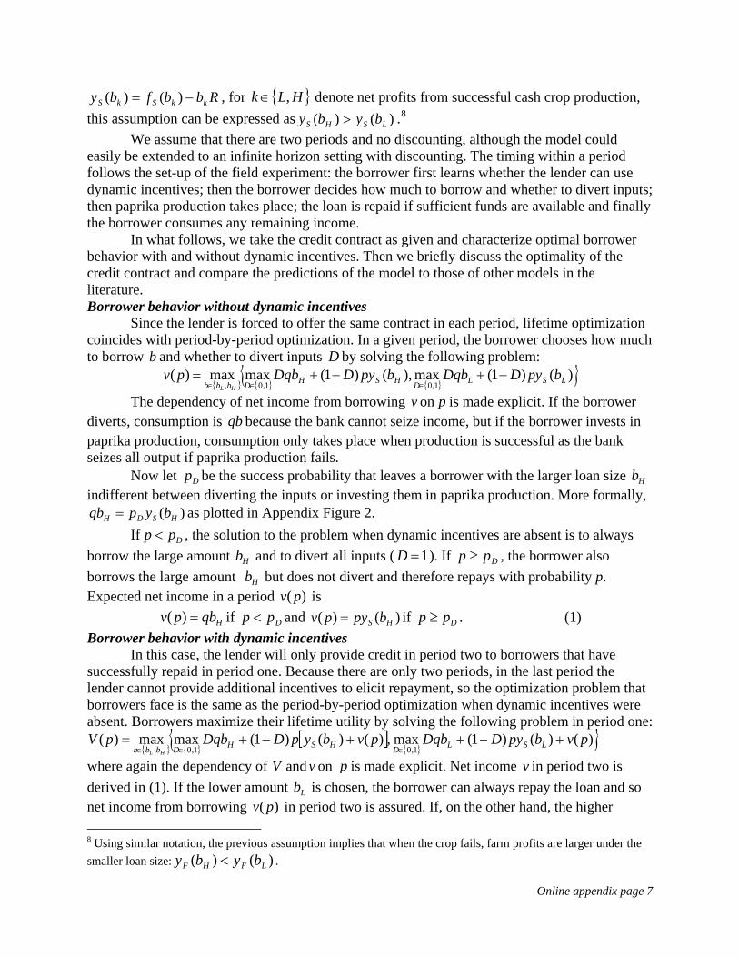
We assume that there are two periods and no discounting, although the model could easily be extended to an infinite horizon setting with discounting. The timing within a period follows the set-up of the field experiment: the borrower first learns whether the lender can use dynamic incentives; then the borrower decides how much to borrow and whether to divert inputs; then paprika production takes place; the loan is repaid if sufficient funds are available and finally the borrower consumes any remaining income.

In what follows, we take the credit contract as given and characterize optimal borrower behavior with and without dynamic incentives. Then we briefly discuss the optimality of the credit contract and compare the predictions of the model to those of other models in the literature. Borrower behavior without dynamic incentives

Since the lender is forced to offer the same contract in each period, lifetime optimization coincides with period-by-period optimization. In a given period, the borrower chooses how much to borrow b and whether to divert inputs D by solving the following problem:

{ } { }{ }{ })()1(max),

1,0, LSLDbbpyDDqb

H

()1( HS bpyDmax1,0 HD

Dqbmax)(bb

pvL

−+=∈

−+ ∈ ∈

The dependency of net income from borrowing v on p is made explicit. If the borrower diverts, consumption is because the bank cannot seize income, but if the borrower invests in paprika production, consumption only takes place when production is successful as the bank seizes all output if paprika production fails.

qb

Now let be the success probability that leaves a borrower with the larger loan size indifferent between diverting the inputs or investing them in paprika production. More formally,

as plotted in Appendix Figure 2.

Dp

)( HSDH bypqb =

Dpp <

Hb

If , the solution to the problem when dynamic incentives are absent is to always borrow the large amount b and to divert all inputs (H 1=D ). If , the borrower also borrows the large amount but does not divert and therefore repays with probability p. Expected net income in a period is

Dpp ≥

Hb)( pv

Dpp <Hqbpv =)( if . (1) Dpp ≥)()( HS bpypv =if and Borrower behavior with dynamic incentives

In this case, the lender will only provide credit in period two to borrowers that have successfully repaid in period one. Because there are only two periods, in the last period the lender cannot provide additional incentives to elicit repayment, so the optimization problem that borrowers face is the same as the period-by-period optimization when dynamic incentives were absent. Borrowers maximize their lifetime utility by solving the following problem in period one:

{ } { }{ }[ ]

{ })()()1(max

1,01,0,pvbpyDDqb LSLDHDbbb HL

+,)()( pvbH)1( ypD Smaxmax)( DqbpV = +−+∈∈∈

−+

where again the dependency of and on V v p is made explicit. Net income in period two is derived in (1). If the lower amount b is chosen, the borrower can always repay the loan and so

v

L

net income from borrowing )( pv in period two is assured. If, on the other hand, the higher

)()( LFHF byby <

8 Using similar notation, the previous assumption implies that when the crop fails, farm profits are larger under the smaller loan size: .


amount Hb is chosen, then th rower will obtain )( pv in period two only if there is no diversion 0=D ) and paprika production is success period one. Income from not borrowing is normalized to zero.

It is easy to see that with d

e bor ( ful in

ynamic incentives, diversion of inputs in the first period is never o

ore ptimal. A borrower with a high probability of success Dpp ≥ would not divert in the

absence of penalties, so he would certainly not do it when the can impose penalties. Mformally, because HHS qbbpy >)( if Dpp ≥ , it follows that

lender[ ] HHS qbpvbyp >+ )()( since

0)( >pv . When p < Dp , borrowers choose to divert in the absence of dynamic incentives. When

dynami

. Let 0Bp be the probability of success

c incentives are in place, they can increase lifetime utility by choosing the lower amountin the first period. They then secure a loan in the second period which can then be diverted to achieve the same utility as if they had diverted in the first period. In addition, if cash crop production succeeds, then they also consume in the first period.9

We now study the choice of loan amount in the first period that leaves a borrower with success probability Dpp ≥ indifferent between the two loan

amounts. If success probability is such that D ppp 0B<< , then the borrower chooses Lb to ensure loan repayment, but if the probability is high enough, so that ppp BD << 0 he then chooses Hb . The subscript 0 denotes the fact that in the absence of dy ives the borrower ould not divert because Dpp ≥ . Probability 0Bp can be written as

n incentamic w

)(0HS by

be analogous to 0Bp

)( LS byp = . (2B

Now let D

c incentives. If

)

1Bp for borrowers with success probability pp < . Here the subscript 1 indicates that the b ower would divert in the absence of dynsuccess probability satisfies DB ppp

orr ami<< 1 , the borrower will choose the smaller loan amount

and if DB ppp <<1 the larg . It is easy to show that 1Bp satisfies [ ])(() 11 LSHSBB bybypp

Lb er amount Hb

)1(Hqb −=− (3) or, after some algebra and substitutions,

01

DB

pp = . 1 BD pp −+

(4)

out, depending on L HS H 1BD p> or

D pp <

e )( HS by> mwh

S

yAs it

than the gains from

turns

relevant. There are three cases, wh

The first cas

the magnitude of )(by , )(by and qb only p

0B will hold, because 1BD pp > is true if and onl D if p

, in which the gains fen the high loan am

0Bp> .10

ro

So either 0Bp s we label (i), (ii), and (iii), distinguished by the size of the

gains from input diversion ( Hqb ) relative to those from successful cash crop production, )( HS byand )( LS by .

or 1Bp iich

Hqb cash crop production even

is where (i) diversion are higher ount is taken and

1Bp

9 While this result is immediate without discounting, it can be obtained with discounting provided the discount rate is low enough. 10 This is easy to see using the expression for derived in (4).


producrepay

nt

tion is successful. In this ca 01 BB pp > and 0Bp becomes irrelevant because

0BD pp < is violated. Intuitively, 1>Dp means that there are no borrowers who would without dynamic incentives, because th rsion are higher than the gains from

production even for borr with the highest success probabilities; 0Bp is irrelevabecause there are no farmers for whom Dpp > . In the first period with dynamic incentives, borrowers with 1Bpp ≥ take the larger loan and those for whom 1Bpp

se, 1Dp >>

e gains frowers

om divecash crop

< take the smaller loan size.

The second – and probably most interesting – case is wher )()( LSHHS byqbb >> , in wh

e (ii) yich the gains from diversion (r ash are intermediate. In this

case, in

n ttaken. H h

vant. Probability 1Bp is shown as the intersection of the left hand side and right ha

r im ic

they

ives and not divert with incentives.

elative to c crop production) the absence of dynamic incentives, some borrowers (those with

probabilities, for whom Dpp > ) will choose to produce rather than divert, while others with lower success probabilities will divert rather than produce. In this case we have

011 BBD ppp >>> ,

highest success

n

1Bp≥ take the

rsion arehe small loan size is

11 an 0 is irrelevant (those with Dpp > always choose the larger loain the first period). In the first period with dynamic incentives, borrowers with p

1Bpp < take the smaller loan size. The third case is where (iii) HLS qbby >)( , in which the gains from dive small

relative to the gains from succes h crop production, even whe

d so Bp

larger loan and those for whom

sful casere, DBB ppp >>> 101 so th ecomes irrelevant (because all individuals wit

Dpp < will take the smaller loan size in the first period with dynamic incentives). Now it isthose borrow Dp that w variation in loan size in the first period with

incentives: those with 0Bpp ≥ take the larger loan and those for whom 0Bpp < takethe smaller loan size.

Appendix Figure 2 is drawn assuming Case (ii) holds. It plots 0Bp and Bp

0BD pp > , 0Bp is irrele

at 1Bp now b

shoers for whom p >dynamic

1 , and because

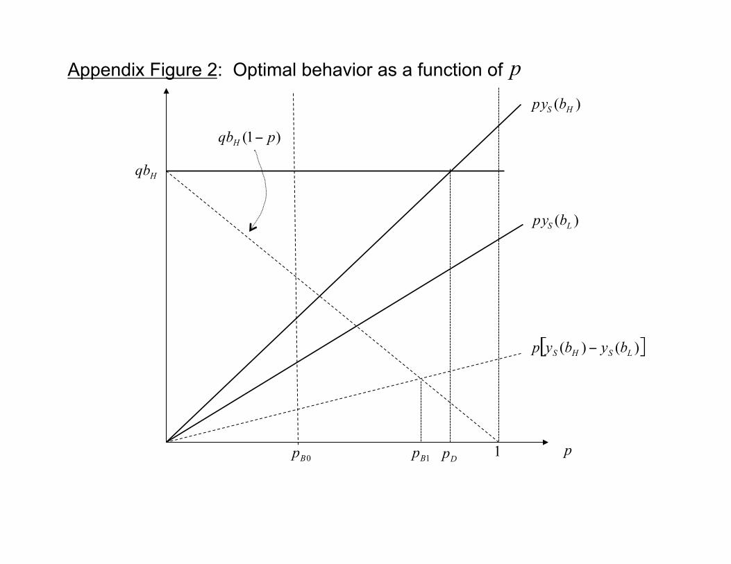
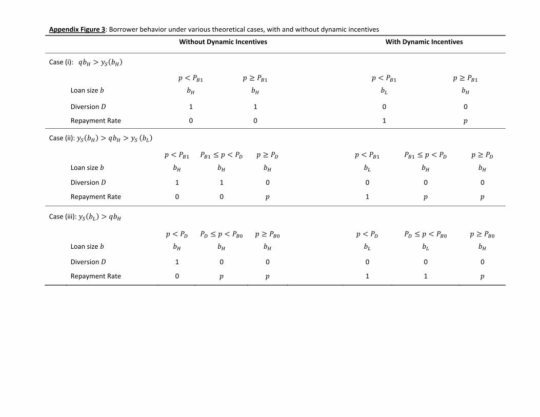
nd side of the equality in (3) above. F eg e (with and without dynam incentives), Appendix Figure 3 reports the

first period optimal choices of loan size and whether to divert as well as repayment rate as a function of the borrowers’ success probability.

or each

Interestingly, and as mentioned in the text, dynamic incentives have different effects on the optimal choices of borrowers depending on their probability of success. For example, borrowers with relatively low probability of success are most affected by the introduction of dynamic incentives. They choose the higher loan amount and to divert it all without dynamic incentives but borrow the lower amount and invest it in cash crop production when dynamic incentives are introduced. As a result, their repayment rate changes from zero to one once incentives are introduced.

Borrowers with relatively high probability of success are the least affected, since theynever divert inputs and always choose the higher loan amount, except for in Case (i) wherewould divert without incent

)( HS by )( HSDH bypqb = and expression (4). 11 To see this, divide inequalities in (ii) by and recall


Borrowers with an intermediate value of the probability of success will, upon introduction of dynamic incentives, change either the diversion or the loan size decisions depending on the parameter values and functional forms. In Case (ii) they always choose the higher duced. In

loan

]1,0[∈ is drawn from the density function )( pG , then R satisfies

loan amount but move from diversion to no diversion when incentives are introCase (iii), they never divert but incentives lead them to move from the higher to the loweramount. Discussion

If the lender sets gross interest rate R to break even, and the individual probability of success p

ib )]())|(1()|()][(1[ HFDDDH bfpppERbpppEpG ≥H −+≥−= , (5)

where i i posit rate and ∫=≥1

)|( D pdGpppE . s the de )( pDp

Notice that the bank breaks-even whenever 1<Dpo collect repayment. As a resu

re is an equilibrium.

, otherwise all borrowers would divert lt, there is no interest rate R such

that c i) considered befo

s uccess

and the bank would be unable t ase (

Depending on the parameters, a separating e rium may exist where the lender maximizes borrower welfare subject to breaking even by offering a menu of loan sizes and grosinterest rates. Borrowers with low probability of s

quilib

p may either borrow the large amount and def

break e

r

be

ike collateral. As in their model, the value of long el

).

centives can be used. As a result, overall borrowing could increase, althoug s

ault or borrow the lower amount and produce (again depending on the parameters), borrowers with intermediate probability of success will borrow the lower amount and produce and borrowers with high probability of success will borrow the large amount and produce.12

When dynamic incentives are introduced, the lender can follow a strategy similar to Stiglitz and Weiss (1983) or Boot and Thakor (1994). In words, the lender could lower the interest rate associated with the lower loan size Lb in the second period below the per period

ven interest rate (thereby making a loss) but raise it in the first period so as to satisfy the break even constraint intertemporally. This may be optimal because in the first period the borrower has the added incentive of the promise of a loan in the future, a loan that will be evemore attractive the lower is the interest rate charged.

If collateral was available, then a menu of interest rates and collateral could alwaysoffered in both periods (Bester, 1985). But as Boot and Thakor (1994) point out, dynamic incentives can be more efficient than static incentives l

-term contracting does not arise from the ability to learn the borrower type (in their modall agents are equal) nor from improved risk-sharing (in both models agents are risk neutralLong term relations are valuable because the lender has the ability to punish defaulters and to reward good borrowers.

Because repayment is higher with dynamic incentives, lenders could lower the interestrate and as a result borrowers might borrow more. The lender should also be willing to extend more credit if dynamic in

h borrowers with low probability of success may still borrow less to ensure future accesto loans. This increase in borrowing is also predicted by the more macro literature that tries to

12 The observation that only a unique (pooling) contract exists may be used to rule out parameter combinations where the separating equilibrium is optimal. Of course, other considerations outside the model may be responsible for only observing one contract, even if it is sub-optimal. For example, before the study MRFC gave only a few loans for paprika and so it may still be learning about the optimal contract.


explain the increase in personal bankruptcies over the last few decades as a result of improvements in information technology available to lenders for credit decisions (see for example Livshits, McGee and Tertilt, forthcoming and 2009; Narajabad, 2010 and Sanchez, 2009).

The source of heterogeneity in the model is the probability of success p . If there wheterogeneity in the discount rate, then dynamic incentives would only be relevant for agentsare patie

as that

nt (ie with low enough discount rate). In this alternative model, if borrowers prefer to divert i d

ts

t has no ince

n the absence of dynamic incentives, repayment would be low without gerprinting anwould only increase for agents with low discount rate when fingerprinting is introduced.

In many multi-period models of limited commitment and asymmetric information, agenare not allowed to save because they could borrow and default and subsequently live in autarky by reinvesting the savings (Bulow and Rogoff, 1989). In Boot and Thakor (1994), the agen

fin

ntive to save because the long-term contract provides better-than-market interest rates. In this model without dynamic incentives, agents with high probability of success will not find it profitable to default and save for period 2 either, even if a savings technology were available at rate i . But if the probability is low enough, in particular if p is such that

)()1(

LS

H

byqbi

p−

< ,

then agents would borrow the higher amiod 2 to earn

Boot and Thakor (1994) applies a

ount Hb in period one, divert and hence default and save it into per 1> . When dynamic incentives are allowed, then the same argument of

nd so agents would prefer to borrow again in the second period, i

even if savings technology were available. Appendix E: Checking for loan officer responses to fingerprinting

In this appendix section we describe in further detail the findings that loan officers do not mmarized in Section 5.A.

f the main text). Online Appendix Table 2 examines reports from all loan officers collected in August

percent.

ccuracy of fingerprinted clubs compared to non-fingerprinted ones. Borrow

clubs,

appear to have responded to whether or not a club was fingerprinted (suo

2008 as well as borrower responses in the August 2008 follow-up survey. Loan officers were first asked about the specific treatment status of five clubs randomly selected from the sample of clubs for which they were responsible. They were then asked whether they knew the secretary or president of the club and finally they were asked to estimate the number of loans given out in each club. The first row of the table shows that loan officers had very little knowledge about the actual treatment status of clubs. Only 54 percent of the fingerprinted clubs are reported correctly as being fingerprinted and an even lower 22 percent of non-fingerprintedclubs are reported correctly as such. Pure guesswork would yield an accuracy rate of 50 This evidence alone suggests that loan officers did not take into account treatment status in their interactions with the clubs.

Loan officers know club officers roughly half of the time, and on average misreport the number of loans disbursed to a club by 1.5 loans. More importantly, there are no statistical differences in the reporting a

er reports in the last three rows of the table paint a similar picture. Loan officers are no more likely to visit non-fingerprinted clubs to collect repayment compared to fingerprinted and as a result, members of non-fingerprinted clubs report talking the same number of times to


loan officers as do members of fingerprinted clubs. Finally, they all report finding it relatively easy to contact the loan officer.

The evidence in the table indicates that loan officers did not respond to the treatment. Therefore, we interpret impacts of the treatment as emerging solely from borrowers’ responses being fingerprinted.

to

onal robustness checks Appendix F: Additi

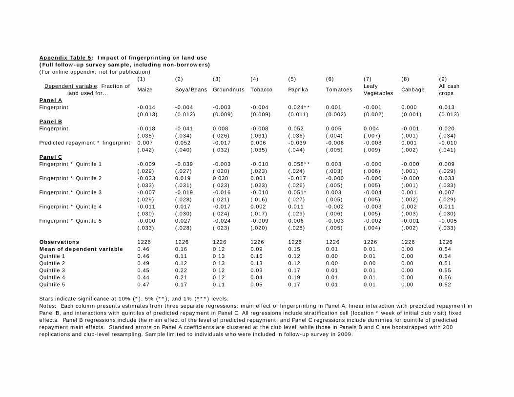
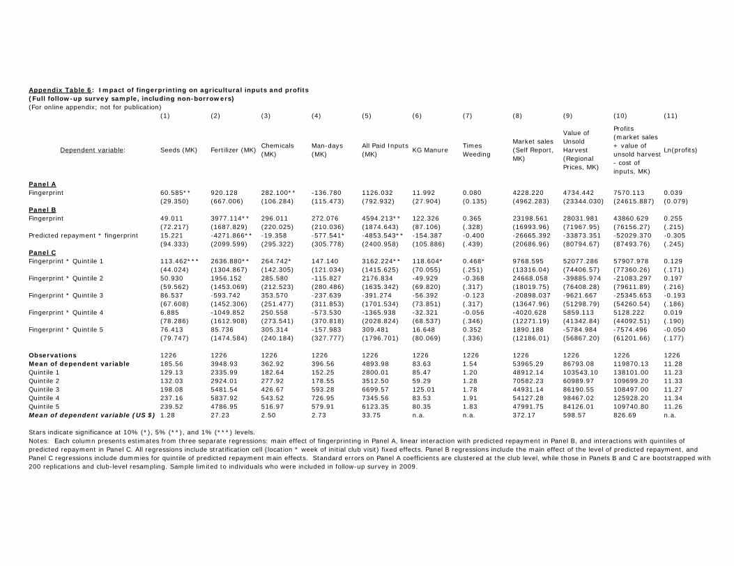
pact of fingerprinting in full sample without restricting the sample only to borrowers,

an help address concerns about selection bias. Appendix Tables 5 and 6 present results from 4 and 5, respectively, with the difference that the

regress

rom

ere significant before to remain statistically significant, but to be only around alf the

ighted

ing

ndix Table 6, Column

term is

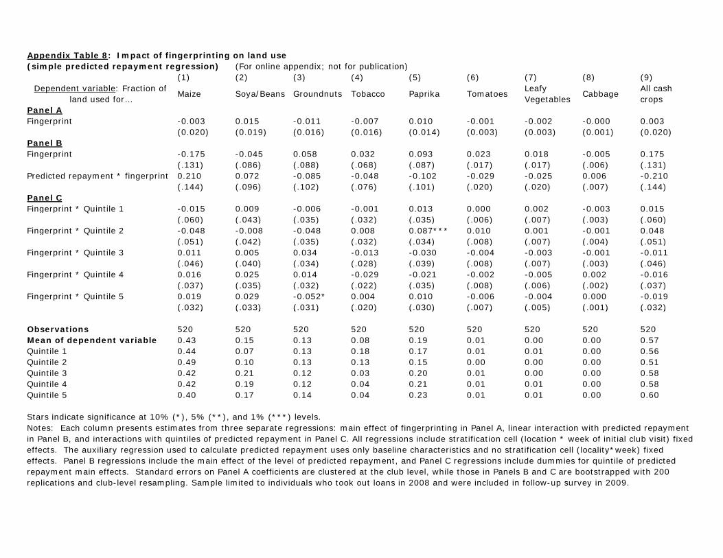
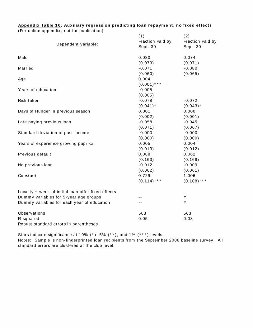
s of treatment effect heterogeneity results to constructing the ment variable when excluding the locality*(week of initial club visit) fixed

on used in the main results (column 3,

dix

ffect. Results from this exercise are presented in Appendix Tables 7 through 9, which should

tical significance in the

Im

Analyses of the full sample of farmers,cregressions analogous to the main Tables

ions include all 1,226 individuals interviewed in the follow-up survey (borrowers plus nonborrowers). Full-sample regression results in Appendix Tables 5 and 6 are very similar to those fthe borrower-only regressions. As discussed in the main text, the general pattern is for coefficients that wh magnitude of the coefficients in the borrowing sample regressions. This reduction in coefficient magnitude is consistent with effect sizes in the full sample representing a weaverage of no effects for nonborrowers and nonzero effects for borrowers.

To be specific, in the land-use full-sample regressions (Appendix Table 5), fingerprintleads farmers in quintile 1 of predicted repayment to devote 5.8 percentage points more of theirland to paprika (significant at the 5% level). In the inputs regressions (Appe

s 1-7), the interaction of fingerprinting with predicted repayment in Panel B is negative and significant at the 5% level in the regressions for fertilizer and all paid inputs, compared to significance at the 10% level in main Table 5. The fingerprinting * (quintile 1) interaction also positive and statistically significant at the 10% level or better for all input types in the table except for man-days. Results in the sales and profits regressions of Appendix Table 6, Columns 8-11 are similar to corresponding ones in main Table 5, but as before they are not statistically significantly different from zero. Results with “simple” predicted repayment regression We discuss here robustnespredicted repayeffects. Compared with the predicted repayment regressiTable 2), when (locality)*(week of initial club visit) fixed effects are dropped the R-squared of the regression falls from 0.48 to 0.08. These alternative specifications are reported in AppenTable 10.

This simpler regression is then used to predict repayment for the full sample, and the predicted repayment variable is interacted with treatment to examine heterogeneity in the treatment e

be compared (respectively) to the main Tables 3 through 5. Results are very similar when using this simpler index of predicted repayment. For

example, the coefficients on the interaction between linear predicted repayment and fingerprinting in Panel B remain large in magnitude and retain statis


repaym les of

ant sum, es on

cribes our approach to estimating predicted repayment using a partition f the control group separate from a partition used as a counterfactual for the treatment group in

st ndom

d t

able

11 corr ponds to

e,

inal coefficient is significant, all coefficients in the 95 percent confide

ent and inputs regressions (Appendix Table 7, Columns 4-9, and Appendix Table 9,Columns 1-7, respectively). In Panel C, where fingerprinting is interacted with quintipredicted repayment, a slight difference vis-à-vis previous results is that typically the significinteraction term is (fingerprinting)*(quintile 2) rather than the interaction with quintile 1. In the general pattern that fingerprinting has more substantial effects on repayment and activitithe farm for individuals with lower predicted repayment is robust to using this simpler predicted repayment regression. Results where predicted repayment coefficients obtained from partition of control group This section desothe main regressions. We conduct this exercise 1,000 times, where in each replication we firra ly select 50% of the control group for inclusion in the auxiliary regression to predict repayment. We then predict repayment for the other half of the control group and the full treatment group. Finally, we estimate the heterogeneous effects of treatment on repayment, lanuse, input use, and farm profits using equation (2) on a sample that includes the full treatmengroup and the half of the control group not randomly chosen for the auxiliary regression.

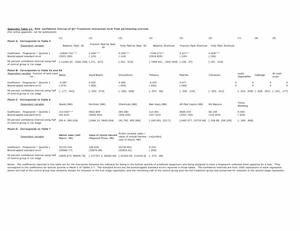
We report the 95 percent confidence interval for coefficients obtained from this procedure in Appendix Table 11. We focus on results for the interaction between the treatmentindicator and the indicator for quintile 1 of predicted repayment.13 Panel A of Appendix T

esponds to Table 3, Columns 4-9; Panel B corresponds to Table 4; Panel C corresTable 5, Columns 1-7, and Panel D corresponds to Table 5, Columns 8-11. The coefficient and standard error reported are the original estimates and bootstrap replications using the full samplas described previously.

In every case, the coefficient from the estimate using the full sample falls within the 95 percent confidence interval from the procedure using the partitioned sample. Furthermore, in every case where the orig

nce interval of the partitioning exercise have the same sign as the coefficient in the mainregressions of the paper, and the confidence interval never includes zero. Appendix G: Details of benefit-cost calculation

The benefit-cost calculation is presented in Appendix Table 13. The uppermost section of l fingerprinted. At the suggestion of MRFC,

e assume that all new loan applicants are fingerprinted, and that 50% of applicants are approv

balance

ted. osts

the table is the calculation of benefits per individuaw

ed for loans. Based on our experimental results we assume that the increase in repayment due to fingerprinting is confined to the first quintile (20% of borrowers), and that for this subgroup fingerprinting causes an increase in repayment amounting to 32.7% of the loan(from column 8 of Table 3). We assume that the total amount to be repaid is MK15,000 on average. Total benefit per individual fingerprinted is therefore MK490.50 (US$3.38). The next section of the table calculates cost per individual fingerprinted. There are three general types of costs. First, equipment costs need to be amortized across farmers fingerprinWe assume each equipment unit (a laptop computer and external fingerprint scanner) c

13 The confidence interval is the 2.5th to 97.5th percentile of coefficients from the 1,000 replications.



new

st of MK19.25 per ustom

which case the fingerprint database is stored on the firm’s server e firm

h fast ven a

MK101,500,14 and is amortized over three years, for annual cost of each equipment package of MK33,833. Twelve (12) of these equipment packages (two for each of six branches) will be required to fingerprint MRFC’s borrowers throughout the country. With an estimated 5,000 loan applicants per year, each of these equipment units will be used to fingerprint 417 farmers onaverage. The equipment cost per farmer fingerprinted is therefore MK81.20. The second type of cost is loan officer time. We estimate that it takes 5 minutes to fingerprint a customer and enter his or her personal information into the database. At a salary of MK40,000 per month and 173.2 work hours per month, this comes out to a coc er fingerprinted. The third type of cost is the transaction cost per fingerprint checked, MK108.75 (US$0.75). We assume here that MRFC hires a private firm to provide the fingerprint identification services, inoverseas and batches of fingerprints to be checked are sent electronically by MRFC to thduring loan processing season. Lists of identified defaulters are sent back to MRFC witturnaround. In consultation with a U.S. private firm that provides such services, we were girange of $0.03-$0.75 per fingerprint identification transaction. Per-fingerprint transaction costs are higher when the client has a relatively low number of transactions per year, and MRFC’s 5,000 transactions per year is considered low, so we conservatively assume the transaction cost per fingerprint at the higher end of this range, $0.75 (MK108.75). Summing up these three types of costs, total cost per individual fingerprinted is MK209.20. The net benefit per individual fingerprinted is therefore MK281.30 (US$1.94), and the benefit-cost ratio is an attractive 2.34. 15

14 This is the actual cost of each equipment unit we purchased for the project, which included a laptop computer ($480), an extra laptop battery ($120), a laptop carrying case ($20), and an external fingerprint scanner ($80). 15 An alternative is for a lending institution to purchase its own fingerprint matching software and do fingerprint identification in-house instead of subcontracting this function to an outside firm. This would eliminate the $0.75 (MK108.75) transaction cost per fingerprint checked. According to a U.S. fingerprint identification services firm we consulted, the initial fixed cost of installing an off-the-shelf fingerprint matching software system is in the range of $15,000 to $50,000 (depending on specifications), with an annual maintenance cost of 10-20% of the initial fixed cost. In addition, there would be personnel costs for staff to operate the system. Assuming an initial fixed cost of $15,000, maintenance cost of 10% of the original fixed cost, and an additional full-time staff member to run the system costing the same as a current MRFC loan officer, NPV is lower when fingerprint identification is done in-house than when this function is contracted out (which is why Appendix Table 13’s calculation assumes contracting out). But with a high enough annual volume of transactions (perhaps in the context of a credit bureau in which many or all of Malawi’s lenders participate), in-house fingerprint identification could make economic sense.

Appendix Figure 1: Experimental Timeline

July 2007

August 2007

Sep. 30, 2008

Clubs organized

Baseline survey and fingerprin@ng begin

November 2007

Loans disbursed

Loans due

April 2008

Input use survey

September 2007

Baseline survey and fingerprin@ng end

Output and profits survey

August 2008

Appendix Figure 2: Optimal behavior as a function of

Appendix Figure 3: Borrower behavior under various theoretical cases, with and without dynamic incentives

Without Dynamic Incentives With Dynamic Incentives

Case (i):

Loan size

Diversion 1 1 0 0

Repayment Rate 0 0 1

Case (ii):

Loan size

Diversion 1 1 0 0 0 0


Case (iii):

Loan size

Diversion 1 0 0 0 0 0


(For online appendix; not for publication)

Mean in control group

Difference in treatment (fingerprinted) group

Mean in control group

Difference in treatment (fingerprinted) group

Variable:

Male 0.81 -0.036 0.80 -0.066*(0.022) (0.037)

Married 0.92 -0.004 0.94 0.003(0.011) (0.016)

Age 39.50 0.019 39.96 -0.088(0.674) (1.171)

Years of education 5.27 -0.046 5.35 -0.124(0.175) (0.272)

Risk taker 0.57 -0.033 0.56 0.013(0.032) (0.051)

Days of hunger in previous season 6.41 -0.647 6.05 -0.292(0.832) (1.329)

Late paying previous loan 0.14 0.005 0.13 0.030(0.023) (0.032)

Standard deviation of past income 25110.62 1289.190 27568.34 -1158.511

Loan recipient sampleFull baseline sample

Appendix Table 1: Tests of balance in baseline characteristics between treatment and control group

(1756.184) (2730.939)

Years of experience growing paprika 2.10 0.096 2.22 0.299(0.142) (0.223)

Previous default 0.03 -0.002 0.02 0.008(0.010) (0.010)

No previous loan 0.74 -0.006 0.74 -0.020(0.027) (0.041)

P-value for test of joint significance 0.91 0.66Observations 3206 1147

Notes: Each row presents mean of a variable in the baseline (September 2008) survey in the control group, and the difference between the treatment group mean and the control group mean of that variable (standard error in parentheses). Differences and standard errors calculated via a regression of the baseline variable on the treatment group indicator; standard errors are clustered at the club level.

Stars indicate significance at 10% (*), 5% (**), and 1% (***) levels.


All Treatment Control

(1) (2) (3) (4) (5)

Loan officer reportsKnows treatment status of club (1=yes) 0.37 0.54 0.22 0.16 51

Knows identity of club officers (1=Yes) 0.47 0.46 0.48 0.88 51

Abs. diff. between actual and officer report of number of loans

1.6 1.3 1.9 0.47 50

Borrower reportsNumber of times loan officer visited club to request loan repayment

0.35 0.41 0.27 0.41 396

Number of times borrower spoke to loan officer since April 2008

2.62 2.57 2.68 0.74 450

Difficulty in locating loan officer (1=easy 2=moderate 3=difficult)

1.2 1.17 1.24 0.32 453

MeansP-value of T-

test of (2)=(3) Num. of obs.

Notes: The first three rows present loan officer reports about knowledge of clubs and treatment status collected in August 2008. The last three rows present borrower reports about interactions with the loan officer collected in the follow-up survey of August 2008.

Appendix Table 2: Impact of fingerprinting on loan officer knowledge and behavior


(1) (2)

Sample: All respondents Loan recipients

Panel AFingerprint -0.062* -0.092

(0.036) (0.069)Panel BFingerprint -0.046 -0.085

(.096) (.167)Predicted repayment * fingerprint -0.021 -0.008

(.118) (.192)Panel CFingerprint * Quintile 1 -0.032 -0.172

(.075) (.129)Fingerprint * Quintile 2 -0.074 0.015 (.073) (.107)Fingerprint * Quintile 3 -0.068 -0.094

(.070) (.107)Fingerprint * Quintile 4 -0.089 -0.089

(.078) (.124)Fingerprint * Quintile 5 -0.090 -0.137

Dependent variable: Indicator for attrition from September 2008 baseline survey to August 2009 survey

Appendix Table 3: Impact of fingerprinting on attrition from sample

Fingerprint Quintile 5 0.090 0.137 (.072) (.125)

Observations 3206 1147Mean of dependent variable 0.63 0.55Quintile 1 0.58 0.59Quintile 2 0.57 0.54Quintile 3 0.63 0.58Quintile 4 0.60 0.50Quintile 5 0.70 0.52

Notes: Each column presents estimates from three separate regressions: main effect of fingerprinting in Panel A, linear interaction with predicted repayment in Panel B, and interactions with quintiles of predicted repayment in Panel C. All regressions include stratification cell (location * week of initial club visit) fixed effects. Panel B regressions include the main effect of the level of predicted repayment, and Panel C regressions include dummies for quintile of predicted repayment main effects. Standard errors on Panel A coefficients are clustered at the club level, while those in Panels B and C are bootstrapped with 200 replications and club-level resampling.


Appendix Table 4: Impact of fingerprinting on loan repayment (Only borrowers responding to follow-up survey)

(1) (2) (3) (4) (5) (6)

Sample:

Loan recipients included in August 2009 survey






Dependent variable: Balance, Sept. 30

Fraction Paid by Sept. 30

Fully Paid by Sept. 30

Balance, Eventual

Fraction Paid, Eventual

Fully Paid, Eventual

Panel AFingerprint -1529.644* 0.063 0.079 -875.314 0.031 0.060

(884.322) (0.043) (0.069) (670.297) (0.032) (0.057)Panel BFingerprint -15727.893*** 0.713*** 0.794*** -8931.946* 0.362 0.390

(3782.488) (.196) (.213) (5162.708) (.237) (.257)Predicted repayment * fingerprint 17587.934*** -0.805*** -0.887*** 10046.221* -0.413* -0.411

(4018.014) (.206) (.240) (5446.717) (.250) (.284)Panel CFingerprint * Quintile 1 -12602.785*** 0.573*** 0.616*** -8016.543* 0.334* 0.373*

(3969.935) (.190) (.197) (4382.064) (.201) (.205)Fingerprint * Quintile 2 1538.937 -0.094 -0.069 1799.143 -0.104 -0.090 (2111.189) (.110) (.166) (1857.158) (.099) (.151)Fingerprint * Quintile 3 -364.091 0.021 0.046 -586.977 0.032 0.062

(891.085) (.051) (.101) (792.850) (.046) (.095)Fingerprint * Quintile 4 560.375 -0.038 -0.085 549.532 -0.033 -0.034


(762.879) (.044) (.103) (707.901) (.041) (.096)Fingerprint * Quintile 5 454.471 -0.022 0.002 289.061 -0.008 0.044 (814.791) (.046) (.104) (674.962) (.038) (.090)

Observations 520 520 520 520 520 520Mean of dependent variable 2071.21 0.89 0.79 1439.16 0.92 0.83Quintile 1 6955.67 0.62 0.52 3472.29 0.83 0.71Quintile 2 4024.05 0.77 0.63 2610.41 0.85 0.75Quintile 3 1571.44 0.92 0.83 476.63 0.97 0.91Quintile 4 877.80 0.95 0.85 661.79 0.96 0.86Quintile 5 1214.19 0.94 0.85 311.66 0.98 0.93

Stars indicate significance at 10% (*), 5% (**), and 1% (***) levelNotes: Each column presents estimates from three separate regressions: main effect of fingerprinting in Panel A, linear interaction with predicted repayment in Panel B, and interactions with quintiles of predicted repayment in Panel C. All regressions include stratification cell (location * week of initial club visit) fixed effects. Panel B regressions include the main effect of the level of predicted repayment, and Panel C regressions include dummies for quintile of predicted repayment main effects. Standard errors on Panel A coefficients are clustered at the club level, while those in Panels B and C are bootstrapped with 200 replications and club-level resampling. Sample limited to individuals who took out loans in 2008 and were included in follow-up survey in 2009.

(Full follow-up survey sample, including non-borrowers)

(1) (2) (3) (4) (5) (6) (7) (8) (9)Dependent variable: Fraction of

land used for…Maize Soya/Beans Groundnuts Tobacco Paprika Tomatoes

Leafy Vegetables

CabbageAll cash crops

Panel AFingerprint -0.014 -0.004 -0.003 -0.004 0.024** 0.001 -0.001 0.000 0.013

(0.013) (0.012) (0.009) (0.009) (0.011) (0.002) (0.002) (0.001) (0.013)Panel BFingerprint -0.018 -0.041 0.008 -0.008 0.052 0.005 0.004 -0.001 0.020

(.035) (.034) (.026) (.031) (.036) (.004) (.007) (.001) (.034)Predicted repayment * fingerprint 0.007 0.052 -0.017 0.006 -0.039 -0.006 -0.008 0.001 -0.010

(.042) (.040) (.032) (.035) (.044) (.005) (.009) (.002) (.041)Panel CFingerprint * Quintile 1 -0.009 -0.039 -0.003 -0.010 0.058** 0.003 -0.000 -0.000 0.009

(.029) (.027) (.020) (.023) (.024) (.003) (.006) (.001) (.029)Fingerprint * Quintile 2 -0.033 0.019 0.030 0.001 -0.017 -0.000 -0.000 -0.000 0.033 (.033) (.031) (.023) (.023) (.026) (.005) (.005) (.001) (.033)Fingerprint * Quintile 3 -0.007 -0.019 -0.016 -0.010 0.051* 0.003 -0.004 0.001 0.007

(.029) (.028) (.021) (.016) (.027) (.005) (.005) (.002) (.029)Fingerprint * Quintile 4 -0.011 0.017 -0.017 0.002 0.011 -0.002 -0.003 0.002 0.011

(.030) (.030) (.024) (.017) (.029) (.006) (.005) (.003) (.030)Fingerprint * Quintile 5 -0.000 0.027 -0.024 -0.009 0.006 -0.003 -0.002 -0.001 -0.005 (.033) (.028) (.023) (.020) (.028) (.005) (.004) (.002) (.033)

Appendix Table 5: Impact of fingerprinting on land use


Observations 1226 1226 1226 1226 1226 1226 1226 1226 1226Mean of dependent variable 0.46 0.16 0.12 0.09 0.15 0.01 0.01 0.00 0.54Quintile 1 0.46 0.11 0.13 0.16 0.12 0.00 0.01 0.00 0.54Quintile 2 0.49 0.12 0.13 0.13 0.12 0.00 0.00 0.00 0.51Quintile 3 0.45 0.22 0.12 0.03 0.17 0.01 0.01 0.00 0.55Quintile 4 0.44 0.21 0.12 0.04 0.19 0.01 0.01 0.00 0.56Quintile 5 0.47 0.17 0.11 0.05 0.17 0.01 0.01 0.00 0.52

Notes: Each column presents estimates from three separate regressions: main effect of fingerprinting in Panel A, linear interaction with predicted repayment in Panel B, and interactions with quintiles of predicted repayment in Panel C. All regressions include stratification cell (location * week of initial club visit) fixed effects. Panel B regressions include the main effect of the level of predicted repayment, and Panel C regressions include dummies for quintile of predicted repayment main effects. Standard errors on Panel A coefficients are clustered at the club level, while those in Panels B and C are bootstrapped with 200 replications and club-level resampling. Sample limited to individuals who were included in follow-up survey in 2009.


(Full follow-up survey sample, including non-borrowers)(For online appendix; not for publication)

(1) (2) (3) (4) (5) (6) (7) (8) (9) (10) (11)

Dependent variable: Seeds (MK) Fertilizer (MK)Chemicals (MK)

Man-days (MK)

All Paid Inputs (MK)

KG ManureTimes Weeding

Market sales (Self Report, MK)

Value of Unsold Harvest (Regional Prices, MK)

Profits (market sales + value of unsold harvest - cost of inputs, MK)

Ln(profits)

Panel AFingerprint 60.585** 920.128 282.100** -136.780 1126.032 11.992 0.080 4228.220 4734.442 7570.113 0.039

(29.350) (667.006) (106.284) (115.473) (792.932) (27.904) (0.135) (4962.283) (23344.030) (24615.887) (0.079)Panel BFingerprint 49.011 3977.114** 296.011 272.076 4594.213** 122.326 0.365 23198.561 28031.981 43860.629 0.255

(72.217) (1687.829) (220.025) (210.036) (1874.643) (87.106) (.328) (16993.96) (71967.95) (76156.27) (.215)Predicted repayment * fingerprint 15.221 -4271.866** -19.358 -577.541* -4853.543** -154.387 -0.400 -26665.392 -33873.351 -52029.370 -0.305

(94.333) (2099.599) (295.322) (305.778) (2400.958) (105.886) (.439) (20686.96) (80794.67) (87493.76) (.245)Panel CFingerprint * Quintile 1 113.462*** 2636.880** 264.742* 147.140 3162.224** 118.604* 0.468* 9768.595 52077.286 57907.978 0.129

(44.024) (1304.867) (142.305) (121.034) (1415.625) (70.055) (.251) (13316.04) (74406.57) (77360.26) (.171)Fingerprint * Quintile 2 50.930 1956.152 285.580 -115.827 2176.834 -49.929 -0.368 24668.058 -39885.974 -21083.297 0.197 (59.562) (1453.069) (212.523) (280.486) (1635.342) (69.820) (.317) (18019.75) (76408.28) (79611.89) (.216)Fingerprint * Quintile 3 86.537 -593.742 353.570 -237.639 -391.274 -56.392 -0.123 -20898.037 -9621.667 -25345.653 -0.193

(67.608) (1452.306) (251.477) (311.853) (1701.534) (73.851) (.317) (13647.96) (51298.79) (54260.54) (.186)Fi i t * Q i til 4 6 885 1049 852 250 558 573 530 1365 938 32 321 0 056 4020 628 5859 113 5128 222 0 019

Appendix Table 6: Impact of fingerprinting on agricultural inputs and profits

Fingerprint * Quintile 4 6.885 -1049.852 250.558 -573.530 -1365.938 -32.321 -0.056 -4020.628 5859.113 5128.222 0.019(78.286) (1612.908) (273.541) (370.818) (2028.824) (68.537) (.346) (12271.19) (41342.84) (44092.51) (.190)

Fingerprint * Quintile 5 76.413 85.736 305.314 -157.983 309.481 16.648 0.352 1890.188 -5784.984 -7574.496 -0.050 (79.747) (1474.584) (240.184) (327.777) (1796.701) (80.069) (.336) (12186.01) (56867.20) (61201.66) (.177)

Observations 1226 1226 1226 1226 1226 1226 1226 1226 1226 1226 1226Mean of dependent variable 185.56 3948.93 362.92 396.56 4893.98 83.63 1.54 53965.29 86793.08 119870.13 11.28Quintile 1 129.13 2335.99 182.64 152.25 2800.01 85.47 1.20 48912.14 103543.10 138101.00 11.23Quintile 2 132.03 2924.01 277.92 178.55 3512.50 59.29 1.28 70582.23 60989.97 109699.20 11.33Quintile 3 198.08 5481.54 426.67 593.28 6699.57 125.01 1.78 44931.14 86190.55 108497.00 11.27Quintile 4 237.16 5837.92 543.52 726.95 7345.56 83.53 1.91 54127.28 98467.02 125928.20 11.34Quintile 5 239.52 4786.95 516.97 579.91 6123.35 80.35 1.83 47991.75 84126.01 109740.80 11.26Mean of dependent variable (US $) 1.28 27.23 2.50 2.73 33.75 n.a. n.a. 372.17 598.57 826.69 n.a.

Notes: Each column presents estimates from three separate regressions: main effect of fingerprinting in Panel A, linear interaction with predicted repayment in Panel B, and interactions with quintiles of predicted repayment in Panel C. All regressions include stratification cell (location * week of initial club visit) fixed effects. Panel B regressions include the main effect of the level of predicted repayment, and Panel C regressions include dummies for quintile of predicted repayment main effects. Standard errors on Panel A coefficients are clustered at the club level, while those in Panels B and C are bootstrapped with 200 replications and club-level resampling. Sample limited to individuals who were included in follow-up survey in 2009.


(For online appendix; not for publication)(1) (2) (3) (4) (5) (6) (7) (8) (9)

Sample: All Respondents All Respondents Loan Recipients Loan recipients Loan recipients Loan recipients Loan recipients Loan recipientLoan recipients

Dependent variable: Approved Any Loan Total Borrowed (MK) Balance, Sept. 30 Fraction Paid by

Sept. 30Fully Paid by Sept. 30

Balance, Eventual



Panel AFingerprint 0.045 0.056 -692.743* -1489.945* 0.069* 0.088 -975.181 0.044 0.080

(0.054) (0.045) (381.745) (836.931) (0.041) (0.066) (762.090) (0.037) (0.061)Panel BFingerprint -0.064 0.012 -717.084 -11562.473*** 0.570*** 0.654*** -7303.437** 0.342** 0.423*

(.151) (.146) (2351.208) (3481.01) (.168) (.243) (3428.208) (.169) (.230)Predicted repayment * fingerprint 0.135 0.054 30.107 12415.234*** -0.618*** -0.698*** 7800.066** -0.367** -0.423*

(.171) (.176) (2656.956) (3947.51) (.185) (.261) (3817.025) (.185) (.246)Panel CFingerprint * Quintile 1 0.023 0.069 125.465 -2550.686* 0.138* 0.147 -1258.495 0.065 0.086

(.073) (.062) (837.873) (1494.379) (.076) (.101) (1454.586) (.074) (.097)Fingerprint * Quintile 2 0.036 0.041 -1193.165* -3306.017** 0.149** 0.204** -2516.761* 0.120* 0.178* (.070) (.063) (699.703) (1538.999) (.075) (.102) (1456.644) (.071) (.100)Fingerprint * Quintile 3 0.076 0.032 -1790.115*** -1819.843 0.060 0.110 -1190.697 0.026 0.112

(.070) (.068) (673.809) (1259.105) (.065) (.100) (1198.203) (.061) (.096)Fingerprint * Quintile 4 0.031 0.053 -311.359 -391.905 0.026 0.003 -423.401 0.028 0.039

(.070) (.063) (663.88) (1089.182) (.054) (.085) (969.012) (.048) (.075)Fingerprint * Quintile 5 0.054 0.085 -263.503 337.027 -0.013 -0.010 304.142 -0.006 -0.002 (.070) (.068) (590.087) (979.543) (.044) (.072) (893.653) (.040) (.068)

Appendix Table 7: Impact of fingerprinting on borrowing and repayment(simple predicted repayment regression)


Stars indicate significance at 10% (*), 5% (**), and 1% (***) levels.Notes: Each column presents estimates from three separate regressions: main effect of fingerprinting in Panel A, linear interaction with predicted repayment in Panel B, and interactions with quintiles of predicted repayment in Panel C. All regressions include stratification cell (location * week of initial club visit) fixed effects. The auxiliary regression used to calculate predicted repayment uses only baseline characteristics and no stratification cell (locality*week) fixed effects. Panel B regressions include the main effect of the level of predicted repayment, and Panel C regressions include dummies for quintile of predicted repayment main effects. Standard errors on Panel A coefficients are clustered at the club level, while those in Panels B and C are bootstrapped with 200 replications and club-level resampling.

(For online appendix; not for publication)(1) (2) (3) (4) (5) (6) (7) (8) (9)

Dependent variable: Fraction of land used for…

Maize Soya/Beans Groundnuts Tobacco Paprika TomatoesLeafy Vegetables

CabbageAll cash crops

Panel AFingerprint -0.003 0.015 -0.011 -0.007 0.010 -0.001 -0.002 -0.000 0.003

(0.020) (0.019) (0.016) (0.016) (0.014) (0.003) (0.003) (0.001) (0.020)Panel BFingerprint -0.175 -0.045 0.058 0.032 0.093 0.023 0.018 -0.005 0.175

(.131) (.086) (.088) (.068) (.087) (.017) (.017) (.006) (.131)Predicted repayment * fingerprint 0.210 0.072 -0.085 -0.048 -0.102 -0.029 -0.025 0.006 -0.210

(.144) (.096) (.102) (.076) (.101) (.020) (.020) (.007) (.144)Panel CFingerprint * Quintile 1 -0.015 0.009 -0.006 -0.001 0.013 0.000 0.002 -0.003 0.015

(.060) (.043) (.035) (.032) (.035) (.006) (.007) (.003) (.060)Fingerprint * Quintile 2 -0.048 -0.008 -0.048 0.008 0.087*** 0.010 0.001 -0.001 0.048 (.051) (.042) (.035) (.032) (.034) (.008) (.007) (.004) (.051)Fingerprint * Quintile 3 0.011 0.005 0.034 -0.013 -0.030 -0.004 -0.003 -0.001 -0.011

(.046) (.040) (.034) (.028) (.039) (.008) (.007) (.003) (.046)Fingerprint * Quintile 4 0.016 0.025 0.014 -0.029 -0.021 -0.002 -0.005 0.002 -0.016

(.037) (.035) (.032) (.022) (.035) (.008) (.006) (.002) (.037)Fingerprint * Quintile 5 0.019 0.029 -0.052* 0.004 0.010 -0.006 -0.004 0.000 -0.019 (.032) (.033) (.031) (.020) (.030) (.007) (.005) (.001) (.032)

Appendix Table 8: Impact of fingerprinting on land use(simple predicted repayment regression)

(.032) (.033) (.031) (.020) (.030) (.007) (.005) (.001) (.032)


Stars indicate significance at 10% (*), 5% (**), and 1% (***) levels.Notes: Each column presents estimates from three separate regressions: main effect of fingerprinting in Panel A, linear interaction with predicted repayment in Panel B, and interactions with quintiles of predicted repayment in Panel C. All regressions include stratification cell (location * week of initial club visit) fixed effects. The auxiliary regression used to calculate predicted repayment uses only baseline characteristics and no stratification cell (locality*week) fixed effects. Panel B regressions include the main effect of the level of predicted repayment, and Panel C regressions include dummies for quintile of predicted repayment main effects. Standard errors on Panel A coefficients are clustered at the club level, while those in Panels B and C are bootstrapped with 200 replications and club-level resampling. Sample limited to individuals who took out loans in 2008 and were included in follow-up survey in 2009.

(1) (2) (3) (4) (5) (6) (7) (8) (9) (10) (11)

Dependent variable: Seeds (MK) Fertilizer (MK) Chemicals (MK)

Man-days (MK)

All Paid Inputs (MK) KG Manure Times

Weeding

Market sales (Self Report, MK)


Profits (market sales + value of unsold harvest - cost of inputs, MK)

Ln(profits)

Panel AFingerprint 84.536 1037.378 357.103 -408.599** 1070.419 44.863 0.048 5808.270 3571.446 11457.127 0.043

(54.312) (1297.753) (219.533) (188.581) (1523.582) (37.258) (0.141) (9376.512) (10525.289) (14071.809) (0.094)Panel BFingerprint 282.642 14092.032** 800.605 391.334 15566.614** 101.494 0.421** 125502.791 -1179.320 96410.326 1.257**

(253.064) (5590.066) (940.826) (1444.871) (6469.535) (194.348) (.878) (62693.17) (147854.1) (168129.6) (.638)Predicted repayment * fingerprint -241.402 -15850.798** -537.673 -972.848 -17602.722** -68.915 -0.455** -145347.128 5848.375 -103103.149 -1.476**

(320.704) (6394.114) (1106.397) (1728.811) (7558.463) (231.059) (1.038) (68584.33) (176461.3) (199752.9) (.751)Panel CFingerprint * Quintile 1 205.670** 2417.000 644.153* -336.456 2930.366 -7.355 0.018 23135.413 -6510.534 11781.684 0.012

(90.561) (2457.178) (351.481) (449.350) (2788.066) (72.893) (.341) (24824.16) (41730.85) (51026.79) (.243)Fingerprint * Quintile 2 204.141** 6126.022** 446.949 -130.578 6646.533** 125.404 0.181 35330.984 -3565.416 22466.436 0.491* (103.150) (2513.384) (358.592) (557.157) (2844.721) (85.541) (.320) (23834.69) (48903.95) (55138.88) (.266)Fingerprint * Quintile 3 -80.495 631.003 350.814 -666.700 234.622 50.845 0.072 -6890.835 64018.007 67407.944 0.193

(108.814) (2508.503) (407.558) (591.505) (2912.471) (77.011) (.332) (22716.73) (55893.06) (61100.77) (.236)Fingerprint * Quintile 4 6.115 -1516.096 192.879 -316.185 -1633.287 19.131 0.053 -5737.961 -70057.413 -71136.598 -0.156

(102.324) (2285.521) (448.384) (539.082) (2722.922) (75.269) (.311) (17755.40) (66463.94) (70012.55) (.235)Fingerprint * Quintile 5 114.650 -644.719 306.239 -571.535 -795.364 26.469 -0.011 -8414.109 28216.613 25251.358 -0.215 (122.226) (2285.481) (407.954) (545.700) (2842.941) (80.906) (.299) (14952.61) (57408.41) (61067.75) (.208)

Observations 520 520 520 520 520 520 520 520 520 520 520Mean of dependent variable 247.06 7499.85 671.31 665.98 9084.19 90.84 1.94 65004.30 80296.97 117779.16 11.44Quintile 1 174 13 6721 24 401 30 143 48 7440 15 97 39 1 47 60662 57 82739 24 121222 50 11 36

Appendix Table 9: Impact of fingerprinting on agricultural inputs and profits(simple predicted repayment regression) (For online appendix; not for publication)

Quintile 1 174.13 6721.24 401.30 143.48 7440.15 97.39 1.47 60662.57 82739.24 121222.50 11.36Quintile 2 140.00 6080.46 620.67 238.94 7080.08 39.25 1.55 89028.25 29995.27 91652.71 11.55Quintile 3 269.90 8927.65 674.48 836.98 10709.00 105.73 2.05 57683.74 96247.91 123242.30 11.44Quintile 4 292.07 7649.51 715.08 936.29 9592.95 93.23 2.24 61088.27 104927.50 136467.50 11.45Quintile 5 340.18 8078.58 892.05 1065.18 10375.99 118.13 2.28 56593.43 85817.08 115172.50 11.39Mean of dependent variable (US $) n.a. n.a. n.a. n.a. n.a. n.a. n.a. 464.32 573.55 841.28 n.a.

Stars indicate significance at 10% (*), 5% (**), and 1% (***) levels.Notes: Each column presents estimates from three separate regressions: main effect of fingerprinting in Panel A, linear interaction with predicted repayment in Panel B, and interactions with quintiles of predicted repayment in Panel C. All regressions include stratification cell (location * week of initial club visit) fixed effects. The auxiliary regression used to calculate predicted repayment uses only baseline characteristics and no stratification cell (locality*week) fixed effects. Panel B regressions include the main effect of the level of predicted repayment, and Panel C regressions include dummies for quintile of predicted repayment main effects. Standard errors on Panel A coefficients are clustered at the club level, while those in Panels B and C are bootstrapped with 200 replications and club-level resampling. Sample limited to individuals who took out loans in 2008 and were included in follow-up survey in 2009.

(For online appendix; not for publication)(1) (2)

Dependent variable:Fraction Paid by Sept. 30


Male 0.080 0.074(0.073) (0.071)

Married -0.071 -0.080(0.060) (0.065)

Age 0.004(0.001)***

Years of education -0.005(0.005)

Risk taker -0.078 -0.072(0.041)* (0.043)*

Days of Hunger in previous season 0.001 0.000(0.002) (0.001)

Late paying previous loan -0.058 -0.045(0.071) (0.067)

Standard deviation of past income -0.000 -0.000(0.000) (0.000)

Years of experience growing paprika 0.005 0.004(0.013) (0.012)

Previous default 0.088 0.062(0.163) (0.169)

No previous loan -0.012 -0.009(0.062) (0.061)

Constant 0 729 1 006

Appendix Table 10: Auxiliary regression predicting loan repayment, no fixed effects

Constant 0.729 1.006(0.114)*** (0.108)***

Locality * week of initial loan offer fixed effects -- --Dummy variables for 5-year age groups -- YDummy variables for each year of education -- Y

Observations 563 563R-squared 0.05 0.08Robust standard errors in parentheses

Stars indicate significance at 10% (*), 5% (**), and 1% (***) levels.Notes: Sample is non-fingerprinted loan recipients from the September 2008 baseline survey. All standard errors are clustered at the club level.

Appendix Table 11: 95% confidence interval of Q1*Treatment interaction term from partitioning exercise(For online appendix; not for publication)

(1) (2) (3) (4) (5) (6) (7) (8) (9)Panel A: Corresponds to Table 4

Dependent variable: Balance, Sept. 30 Fraction Paid by Sept. 30

Fully Paid by Sept. 30 Balance, Eventual Fraction Paid, Eventual Fully Paid, Eventual

Coefficient: Fingerprint * Quintile 1 -10844.701*** 0.506*** 0.549*** -7249.271** 0.327** 0.408***Bootstrapped standard error (2622.283) (.125) (.144) (2918.825) (.135) (.156)

95 percent confidence interval using half of control group in 1st stage

[-11284.34, -5382.259] [.271, .527] [.301, .623] [-7999.921, -2937.949] [.138, .37] [.187, .519]

Panel B: Corresponds to Table 5a and 5bDependent variable: Fraction of land used

for…Maize Soya/Beans Groundnuts Tobacco Paprika Tomatoes Leafy

VegetablesCabbage All cash

crops

Coefficient: Fingerprint * Quintile 1 -0.087 0.002 0.005 -0.007 0.077 0 0 0 0Bootstrapped standard error (.074) (.058) (.050) (.050) (.049) 0 0 0 0


[-.177, .041] [-.043, .073] [-.056, .068] [-.097, .06] [-.002, .124] [-.003, .012] [-.015, .008] [-.008, .001] [-.041, .177]

Panel C: Corresponds to Table 6

Dependent variable: Seeds (MK) Fertilizer (MK) Chemicals (MK) Man-days (MK) All Paid Inputs (MK) KG Manure Times Weeding

Coefficient: Fingerprint * Quintile 1 214.555*** 5852.606 384.382 114.901 6566.444 56.139 0.406Bootstrapped standard error (82.610) (4058.444) (339.435) (207.522) (4262.700) (124.425) (.329)


[99.4, 288.319] [1066.13, 9849.334] [91.782, 955.366] [-160.601, 222.7] [1482.077, 10720.66] [-106.88, 158.155] [-.184, .848]

Panel D: Corresponds to Table 7

Market sales (Self Value of Unsold Harvest Profits (market sales +

Dependent variable: Market sales (Self Report, MK)


value of unsold harvest - cost of inputs, MK)

Ln(profits)

Coefficient: Fingerprint * Quintile 1 32123.244 168.559 25730.854 0.434Bootstrapped standard error (39966.77) (33675.88) (53903.61) (.359)


[3835.673, 96839.79] [-127201.3, 46065.56] [-91420.59, 112410.6] [-.072, .98]

Notes: The coefficients reported in this table are for the interaction between the indicator for being in the bottom quintile of predicted repayment and being assigned to have a fingerprint collected when applying for a loan. They correspond to the coefficients for bottom quintile in Panel C of Tables 3-7. The standard errors are the bootstrapped standard errors reported in those tables. The confidence intervals are from 1000 replications of each regression where one half of the control group was randomly chosen for inclusion in the first stage regression, and the remaining half of the control group plus the full treatment group was preserved for inclusion in the second stage regression.

(1) (2) (3) (4) (5) (6)

Dependent variable: Balance, Sept. 30


Fully Paid by Sept. 30

Balance, Eventual



Panel AFingerprint -266.318 0.010 0.001 201.469 -0.012 -0.003

(768.031) (0.040) (0.066) (559.701) (0.030) (0.052)Panel BFingerprint -9659.780* 0.422 0.412 -5190.059 0.198 0.207

(4698.647) (.237) (.298) (5140.761) (.237) (.280)Predicted repayment * fingerprint 11231.990** -0.493 -0.493 6443.577 -0.251 -0.252

(4903.271) (.246) (.326) (5378.012) (.247) (.308)Panel CFingerprint * Quintile 1 -8276.641* 0.372* 0.333 -5247.917 0.221 0.240

(4308.034) (.204) (.246) (4236.123) (.189) (.220)Fingerprint * Quintile 2 2691.144 -0.150 -0.159 2402.793 -0.135 -0.138 (2204.118) (.115) (.164) (1919.401) (.102) (.148)Fingerprint * Quintile 3 -410.867 0.031 0.042 -210.122 0.021 0.037

(1038.583) (.058) (.105) (910.565) (.052) (.096)Fingerprint * Quintile 4 432.743 -0.017 -0.073 650.240 -0.026 -0.067

(872.418) (.050) (0.104) (818.118) (.047) (.095)Fingerprint * Quintile 5 361.559 -0.012 -0.003 614.725 -0.021 0.015 (1004.290) (.055) (.115) (857.018) (.046) (.096)

Observations 520 520 520 520 520 520Mean of dependent variable 2071 21 0 89 0 79 1439 16 0 92 0 83

Appendix Table 12: Ex post moral hazard

Mean of dependent variable 2071.21 0.89 0.79 1439.16 0.92 0.83Quintile 1 6955.67 0.62 0.52 3472.29 0.83 0.71Quintile 2 4024.05 0.77 0.63 2610.41 0.85 0.75Quintile 3 1571.44 0.92 0.83 476.63 0.97 0.91Quintile 4 877.80 0.95 0.85 661.79 0.96 0.86Quintile 5 1214.19 0.94 0.85 311.66 0.98 0.93Comparison to Appendix Table 4Difference in Panel B interaction terms 6355.944** -0.312** -0.394* 4019.440 -0.197* -0.224

(2852.902) (.137) (.205) (2485.785) (.116) (.183)Difference in Quintile 1 interaction terms -4326.144** 0.201** 0.284** -2836.847 0.128 0.163

(2050.553) (.100) (.139) (1758.450) (.084) (.127)

Stars indicate significance at 10% (*), 5% (**), and 1% (***) levels.Notes: Each column presents estimates from three separate regressions: main effect of fingerprinting in Panel A, linear interaction with predicted repayment in Panel B, and interactions with quintiles of predicted repayment in Panel C. All regressions include stratification cell (location * week of initial club visit) fixed effects. Panel B regressions include the main effect of the level of predicted repayment, and Panel C regressions include dummies for quintile of predicted repayment main effects. Standard errors on Panel A coefficients are clustered at the club level, while those in Panels B and C are bootstrapped with 200 replications and club-level resampling. Sample limited to individuals who took out loans in 2008 and who were included in follow-up survey in 2009.

(a) Increase in repayment due to fingerprinting in Quintile 1 4,905.00 Malawi kwacha(b) Quintile 1 as share of all borrowers 20.0%(c) Borrowers as share of all fingerprinted 50%

(d) Total benefit per individual fingerprinted [ = (a)*(b)*(c)] 490.50 Malawi kwacha

(e) Cost per equipment unit 101,500 Malawi kwacha(f) Equipment amortization period 3 years(g) Annual equipment amortization [ = (e) / (f)] 33,833 (h) Fingerprinted individuals per equipment unit 417 individuals(i) Equipment cost per farmer [ = (g) / (h)] 81.20 Malawi kwacha(j) Loan officer time cost per farmer 19.25 Malawi kwacha(k) Transaction cost per fingerprint checked 108.75 Malawi kwacha

(l) Total cost per individual fingerprinted [ = (i) + (j) + (k)] 209.20 Malawi kwacha

281.30 Malawi kwacha2.34

145 MK/US$15 000 Malawi kwacha

Exchange rate:Loan size

Assumptions:

Appendix Table 13: Benefit-cost analysis

Benefit

Cost

(m) Net benefit per fingerprinted farmer [ = (d) - (l)](n) Benefit-cost ratio [ = (d) / (l)]

15,000 Malawi kwacha32.7%

700 USD12

5,000

5 minutes40,000 Malawi kwacha

173.2 hours

Fingerprinting time per individualMonthly salary of MRFC loan officerHours worked per month by MFRC loan officer

Loan sizeIncrease in share of loan repaid due to fingerprinting in Quint

Cost per equipment unit (laptop computer + fingerprint scannNumber of equipment unitsNew loan applicants fingerprinted per year

Documents

Online Appendix Evidence from Malawi Dean Yang Appendix A ...econweb.umd.edu/~goldberg/docs/gine_goldberg_yang... · Background on Cheetah Paprika (CP) Extension services provided