One system reliability assessment methOd fOr cnc grinder metOda

Eksploatacja i NiEzawodNosc – MaiNtENaNcE aNd REliability Vol.16, No. 1, 2014 97

Article citation info:

1. Introduction

CNC grinder is one machine tool which uses the grinding tools to grind or polish the parts’ surface and it is widely applied in the fields of mechanical manufacturing industry, such as aviation and space-flight, vehicles, ship, etc. Because CNC grinder is the last equipment in manufacturing process usually, its stability and reliability is very important. The critical of reliability enhancement of CNC grinder is design and manufacturing, which needs to evaluate current reliability level and find the weak link to redesign. The reliability assessment, estimation or prediction is the important reference to reliability design and the article aims at the reliability assessment method and algorithm for CNC grinder.

Some approaches for reliability assessment have been proposed and a few achievements have been gained. Young KS proposed one method of reliability prediction of engineering system which the sys-tem functionality and system performance are considered [19]. Mo-hammed TL presented one simple reliability-oriented method to cal-culate complex distribution system reliability, which is one simplified method [10]. Nathan G developed one method to predict the reliabil-ity of electronic packages by expert system [13]. Wei-jenn K proposed one reliability evaluation algorithm countering for imperfect nodes in distributed computing networks [8].

Copal C proposed one system reliability calculation algorithm il-lustrated through some well-known structures, such as series, paral-lel, k-out-of-n:G and a fire detector system. The algorithm has been programmed [3]. The difficulty of the algorithm is to solve the struc-ture function. Donald SJ proposed one method to estimate the field-reliability for field-replaceable unit [5]. The estimation model of the method has the merit that the effects of special causes are considered, in addition to the wear of components.

Zunino JL developed the reliability assessment program for MEMS which includes the reliability assessing models and test meth-odologies [20]. Reliability assessment program is described of aero-space electronic equipment by Condra L [4]. Although the program is standardized, the method is not uniform, instead, it is flexible.

Lu H proposed the reliability sensitivity analysis of mechanical parts with failure modes and Guo J proposed one reliability sensitivity analysis method to identify which variable has the highest contribu-tion to system reliability [11, 7].

The traditional estimation or prediction methods have some shortcomings as follows. 1) The fault distribution function principle of subsystems can not be explored and the distribution function of system is random. 2) Reliability estimation for new product needs to be assembled, which needs high cost and long period. 3) The fact that one product is composed of some universal subsystems whose distributions are known by accumulated reliability data was ignored. For the above, one subsystem distribution function fitting and sys-tem MTBF solution method was proposed and the reliability of CNC grinder was assessed by the method.

2. Subsystem distribution function

2.1. Fault data statistic

To find the subsystem’s fault time distribution regularity and then evaluate the subsystem’s reliability level, the reliability experiments and fault data acquisition are necessary, which are the basis of fault time distribution function fitting of subsystems. Enough fault data must be collected for confidence level and the usual method is time curtailed test. The test time is chosen as the maximal of subsystem’s

Liu Y, FAN J, Li Y. One system reliability assessment method for cnc grinder. Eksploatacja i Niezawodnosc – Maintenance and Reliability 2014; 16 (1): 97–104.

Yongjun LiuJinwei FANYun Li

One system reliability assessment methOd fOr cnc grinder

metOda Oceny nieZaWOdnOŚci systemUsZlifierKi cncThe reliability level of CNC (Computer Numerical Control) grinder is usually assessed by fault data counted in laboratory or in field, which needs the grinder to be assembled and it is one afterwards estimation method. To evaluate the reliability level of CNC grinder in design phrase, one system reliability assessment method and algorithm was put forward by subsystem’s reliability in this article, which needs subsystem classification, reliability test, distribution function fitting, parameters estimation and reliability as-sessment. The calculation result showed that the method was feasible and accurate compared with the traditional way. The method is one contribution to reliability design for CNC grinder and is one reference to other mechatronic products.

Keywords: system reliability, assessment method, MTBF, CNC grinder.

Poziom niezawodności szlifierki CNC (sterowanej numerycznie) zazwyczaj ocenia się na podstawie danych o uszkodzeniach liczo-nych w laboratorium lub w terenie, co wymaga zmontowania szlifierki i jest metodą oceny post-factum. Aby umożliwić ocenę po-ziomu niezawodności szlifierki CNC na etapie projektowania, w niniejszym artykule zaproponowano metodę oceny niezawodności systemu oraz odpowiedni algorytm wykorzystujące dane dotyczące niezawodności podsystemów. Model ten wymaga klasyfikacji podsystemów, badań niezawodności, dopasowania funkcji rozkładu, oceny parametrów oraz oceny niezawodności. Wyniki obliczeń wykazały, że omawiana metoda sprawdza się i jest dokładna w porównaniu z metodą tradycyjną. Przedstawiona metoda stanowi wkład do procesu projektowania niezawodności szlifierki CNC i znajduje odniesienie do innych produktów mechatronicznych.

Słowa kluczowe: niezawodność systemu, metoda oceny, MTBF, szlifierka CNC.

Eksploatacja i NiEzawodNosc – MaiNtENaNcE aNd REliability Vol.16, No. 1, 201498

sciENcE aNd tEchNology

MTBF (Mean Time Between Failures). Fault data acquisition should meet the conditions as follows [1].

Only the relevant fault should be counted and the fault caused 1) by experiment condition or human factor should be ignored.The faults caused by one relevant fault should be combined 2) into one fault with the relevant fault.The fault happened at intermitted period and end of experi-3) ment should be counted.

The fault data should be divided into groups by time and the number of groups should be not too big that the probability density will be anamorphic or too small that the calculation load will be heavy and the fitting will be difficult. The number of groups can be calcu-lated by Equation (1) [18].

ˆ 1 3.3ln )ik n= + ∑( (1)

The number of group k can be gained by rounding of k̂ and the fault data statistics table should be drawn as table 1. In table 1, Δti− is the left terminal, Δti+ is the right terminal and ∆ti is the middle of the time

group. ni is the fault number of the ith group and ttest is the test time.

2.2. Distribution type identification

After the fault numbers of every interval were counted, the ob-served value of fault probability density can be calculated by Equation (2). In Equation (2), Δt is the time of each group.

ˆ ( ) ii

i

nf tt n

=∑ÄΔt

(2)

The common probability distributions of mechatronic product are exponential, weibull, normal and logarithmic normal distribution as shown in Fig.1[15]. CNC grinder is one typical mechatronic prod-uct and the probability of its subsystem can be confirmed by plotting

the scatter points and identifying which distribution curve is the most similar.

2.3. Parameters estimation

2.3.1. Least square method [6, 14]

Least square method is the most common method for parameters estimation as its convenience and practicality. Supposing that there are n values {xi, yi}(i=1, 2, … , n), if the relation of x and y is linear and their relation can be fitted by one equation as shown in Equation (3). The parameters a and b can be estimated by Equation (4) using least square method:

ˆ ˆy ax b= + (3)

So, when using the least square method for parameters estima-tion, the linear equation should be created firstly and the parameters in probability density function can be solved by inverse-solving after a and b being calculated by Equation (3). The linear equation creation methods of common distributions are introduced as follows:

1 1

1 1 12

1 1

1

1 1

1

n ni i

i in n n

i i i ii i i

n ni i

i i

ba y xn n

x x y yn n

b

x xn

= =

= = =

= =

= −

− −

= −

∑ ∑

∑ ∑ ∑

∑ ∑

(4)

2.3.2. Normal distribution

Probability density function of normal distribution is shown in Equation (5) and it has two parameters μ and σ [12]:

f t t( ) exp ( )= −

−

12 2

2

2σ πµσ

(5)

The accumulative distribution function meets the relation as shown in Equation (6) if the function is converted to standard normal distribution. The value of F(ti) can be calculated by Equation (7):

F t t zii

i( ) = −

= ( )Φ Φ

µσ

(6)

0

( ) ( )i

i kk

F t f t=

= ∑ (7)

The linear equation can be constructed for normal distribution as shown in Equation (8):

t zi i= +σ µ (8)

In Equation (8), zi is the lower fractile of standard normal distri-bution and can be calculated by inverse function of standard normal distribution. If the sample data meet normal distribution, zi and ti are linear and the observed value of parameters μ and σ can be calculated by Equation (9).

Table 1. Fault data grouping

No. Δti− Δti+ ∆ti ni

1 0 ttest/k ttest/2k n1

2 ttest/k 2ttest/k 3ttest/2k n2

… … … … …

k (k-1)ttest/k ttest (2k-1)ttest/2k nk

Fig. 1. Common probability distribution



µσ==

ba

ˆˆ (9)

2.3.3. Logarithmic normal distribution

Probability density function of logarithmic normal distribution is shown in Equation (10) [2] and it has two parameters μ and σ. The ac-cumulative distribution function meets the relation as shown in Equa-tion (11) if the function is converted to standard normal distribution:

f tt

t( ) exp (ln )= −

−

12 2

2

2σ πµ

σ (10)

F t t zii

i(ln ) ln=

−

= ( )Φ Φ

µσ

(11)

The linear equation can be constructed for logarithmic normal dis-tribution as shown in Equation (12):

ln t zi i= +σ µ (12)

If the sample data meet logarithmic normal distribution, zi and lnti are linear and the observed value of parameters μ and σ can be calculated by Equation (13):

µσ==

ba

ˆˆ

(13)

2.3.4. Exponential distribution

Probability density function of exponential distribution is shown in Equation (14) and it has one parameter λ. The accumulative distribu-tion function of exponential distribution is shown in Equation (15):

f t e t( ) = −λ λ (14)

F t e ii

t( ) = − −1 λ (15)

Taking the logarithm on both sides of the Equation (15) and Equa-tion (16) can be gained. Supposing ln[1 ( )]iy F t= − and ix t= , the linear equation can be created as Equation (17):

ln[ ( )]1− = −F t ti iλ (16)

y x= −λ (17)

So, if the sample data meet exponential distribution, ti and ln[1 ( )]iF t− are linear and the observed value of parameters λ can be calculated by Equation (18).

λ = −aˆ (18)

2.3.5. Weibull distribution

Probability density function of weibull distribution is shown in Equation (19) [9] and it has three parameters m, η and γ. Normally,

it is considered that the product has the probability of fault when the product starts to run. So, parameter γ equals to zero. The accumulative distribution function of two-parameter weibull distribution is shown in Equation (20):

f t m t tm m( ) exp=

−

−

−

−

ηγ

ηγ

η

1

(19)

F t ti im( ) exp[ ( ) ]= − −1 η (20)

Taking the logarithm twice on both sides of the Equation (20) and

Equation (21) can be gained. Supposing 1ln ln1 ( )i

yF t

=−

and

ln ix t= , the linear equation can be created as Equation (22):

ln ln( )

ln ln11−

= −

F tm t m

ii η (21)

y mx m= − lnη (22)

If the sample data meet weibull distribution, 1ln ln1 ( )iF t−

and lnti

are linear and the observed value of parameters m and η can be calcu-lated by Equation (23):

µ

η

=

= −

bab

expˆ

ˆ (23)

2.4. Goodness of fit test

To find the difference of the fitted values and the real values, the fitting effect should be test after the parameters were estimated, and it is called goodness-of-fit test. The aim of goodness of fit test is to test the quality of fitting and it can be marked by R called goodness of fit coefficient which can be solved by Equation (24) [16]:

( )

( )

2

2 1

2

1ˆ

ni

in

ii

y yR

y y

=

=

−=

−

∑

∑ (24)

In Equation (24), yi is the fitted value, ˆiy is the observed value and y is the average of yi. The bigger R is, the better the goodness of fit is. Goodness of fit not only can evaluate the quality of fitting, but also can find the best distribution type when some distributions are meet one sample at the same time.

3. Algorithms

Reliability grade, failure rate and MTBF are the common index for reliability level and MTBF is the most universal. The system MTBF assessment method of CNC grinder was proposed as follow after the subsystem’s distribution functions were fitted.



3.1. Subsystem reliability assessment method

Supposing that the MTBF of exponential distribution, weibull distribution, normal distribution, logarithmic normal distribution are MTBFex, MTBFwb, MTBFnm, MTBFln. MTBF of different distribution can be calculated by its definition (Equation (25)) as shown in Equa-tion (26), Equation (27), Equation (28) and Equation (29). So, the subsystem’s MTBF of CNC grinder can be gained after its probability density function being fitted:

0

= ( )MTBF tf t dt∞∫ (25)

MTBFex =1λ

(26)

MTBFmwb = + +γ ηΓ( )1 1 (27)

MTBFnm = µ (28)

MTBF eln =+( )/µ σ2 2 (29)

3.2. System MTBF solution algorithm

Supposing that there are n subsystems of the CNC grinder and their reliability are signed as MT1, MT2, … , MTn. The system MTBF solution algorithm is proposed as follows.

Sort the subsystem’s 1) MTBF. Vector T is the sorted MTBF of subsystem as shown in Equation (30):

1 2sort( , , , )nMT MT MT=T (30)

Calculate the fault number during truncated time. The trun-2) cated time is the maximum MTBF of subsystem and ki is the rounding value of Tn /Ti as shown in Equation (31):

(1 )ni

i

Tk i nT

= ≤ ≤ (31)

Calculate summary of fault number. 3) θ is the summary of all subsystems’ fault number during truncated time as shown in Equation (32):

θ ==∑kii

n

1 (32)

Calculate the fault time points. 4) tb is the faults time points ma-trix (n×k1) and tbij is the jth fault time point of the ith subsys-tem as shown in Equation (33).

tb =

×

T T k TT T

T n k

1 1 1 1

2 2

22 0

0 01

n

(33)

Calculate system fault time points. System fault time points are 5) the combination of all subsystems’ fault time points. So, if tb tb tb tb= [ ]1 2 n

T (tbi is one row vector), the system

fault time points vector (ts) can be gained by Equation (34):

t tb tb tbs n= [ ]1 2 (34)

Combine all zeros to one. Many zeros exist in 6) ts. Combine all zeros to one and the pure fault time points vector can be got as shown in Equation (35):

tsp t= ≤ ≤[ ] ( )λ λ θ0 (35)

Sort 7) tsp. Sort the vector tsp and the vector t is got as shown in Equation (36) and some critical point can be gained as shown in Equation (37):

t = ≤ ≤ < +[ ] ( , )t m t tm m m0 1θ (36)

tt Tt Tn

0

1 1

0===

θ

(37)

Solve system 8) MTBF. System MTBF signed as MTBFs can be solved by Equation (38) based on its definition:

MTBF

t t

s

ii

i=

−+=∑ ( )1

0

θ

θ (38)

The flow chart of system MTBF solution is shown in Fig. 2 and the total solution can be programmed easily.

3.3. Considering maintenance time

The maintenance time is ignored of system MTBF solution algo-rithm proposed in section 3.2. If the maintenance time is very small compared to subsystem’s MTBF, the ignoring is feasible. Otherwise, the maintenance time must be considered [17]. Supposing that the average maintenance time of subsystem i is tri. Step 1) of section 3.2 should be modified by Equation (39) and the other steps are same:

T = + + +sort( , , , )MT t MT t MT tr r n rn1 1 2 2 (39)

3.4. Considering variety of subsystem’s MTBF

The subsystem’s MTBF variety is not considered in section 3.2. Actually, the subsystem’s MTBF will be decreased along with the in-

Fig. 2. Flow chart of system MTBF solution



creasing of fault number because of wear, deformation, aging and oth-er factors. If the distribution of subsystem is exponential distribution, its MTBF is constant and the subsystem’s MTBF of other distribution type will be varied after maintenance. In earlier time, the difference of MTBF between two maintenances is small and it will become bigger by the increasing of maintenance number. The subsystem’s MTBF is exponential to the number of maintenance. Supposing that the coef-ficient is α, the relation between MTij and MTi1 meets Equation (40):

MT MT eij ij= − − −

111( )( )α (40)

In Equation (40), MTij is the MTBF after j times maintenance of subsystem i. If the subsystem’s distribution is exponential, α is zero. The system MTBF solution method is as follows.

Calculate the fault number. The value of 1) MTij is one geometric progression when i is one fixed value and the fault number j can be solved by Equation (41). ki is the rounded of j:

MTBF j e jt Tij

ri n112 1( )( )− − + ≤− −α (41)

Calculate the faults time points. Considering the subsystem’s 2) MTBF variety and maintenance time, the faults time points matrix can be solved as shown in Equation (42).

tb =

+ + +

+ +

MT t MT t MT t

MT t MT t

MT

r r k r

r r

11 1 12 1 1 1

21 2 22 2

10

0 0

n1

×n k1

(42)

After tb is solved, other calculation steps are same as the above.

4. Reliability assessment

4.1. Subsystems Partition

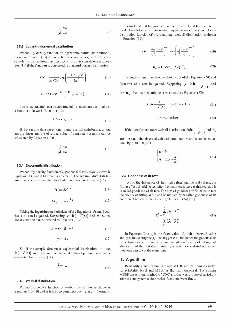
The first step of reliability assessment is subsystem partition. The schematic diagram of one type CNC grinder is illustrated in Fig. 3. The part is clamped between headstock and tail bracket. The part can be rotated around axis of headstock and the grinding wheel can be rotated around axis of spindle. The part’s surface can be grinded as re-

quired by the rectilinear motion and rotatory motion of the headstock and the reciprocating motion of the grinding wheel.

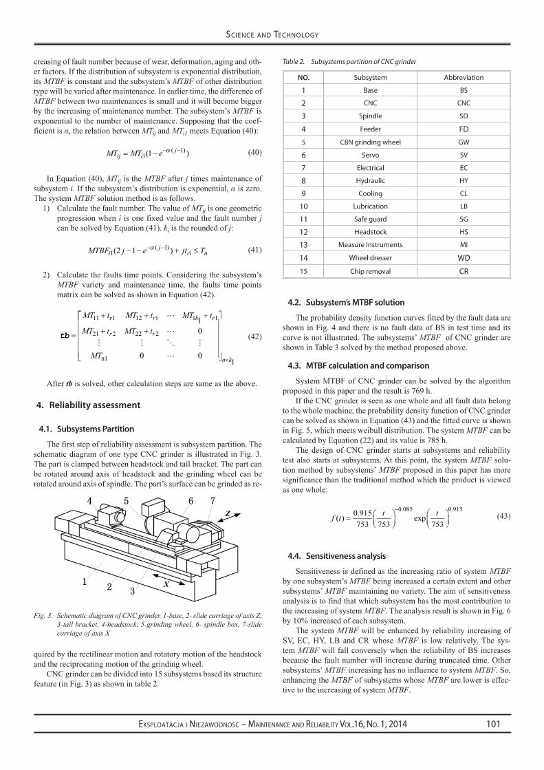
CNC grinder can be divided into 15 subsystems based its structure feature (in Fig. 3) as shown in table 2.

4.2. Subsystem’s MTBF solution

The probability density function curves fitted by the fault data are shown in Fig. 4 and there is no fault data of BS in test time and its curve is not illustrated. The subsystems’ MTBF of CNC grinder are shown in Table 3 solved by the method proposed above.

4.3. MTBF calculation and comparison

System MTBF of CNC grinder can be solved by the algorithm proposed in this paper and the result is 769 h.

If the CNC grinder is seen as one whole and all fault data belong to the whole machine, the probability density function of CNC grinder can be solved as shown in Equation (43) and the fitted curve is shown in Fig. 5, which meets weibull distribution. The system MTBF can be calculated by Equation (22) and its value is 785 h.

The design of CNC grinder starts at subsystems and reliability test also starts at subsystems. At this point, the system MTBF solu-tion method by subsystems’ MTBF proposed in this paper has more significance than the traditional method which the product is viewed as one whole:

0.085 0.9150.915( ) exp

753 753 753t tf t

− =

(43)

4.4. Sensitiveness analysis

Sensitiveness is defined as the increasing ratio of system MTBF by one subsystem’s MTBF being increased a certain extent and other subsystems’ MTBF maintaining no variety. The aim of sensitiveness analysis is to find that which subsystem has the most contribution to the increasing of system MTBF. The analysis result is shown in Fig. 6 by 10% increased of each subsystem.

The system MTBF will be enhanced by reliability increasing of SV, EC, HY, LB and CR whose MTBF is low relatively. The sys-tem MTBF will fall conversely when the reliability of BS increases because the fault number will increase during truncated time. Other subsystems’ MTBF increasing has no influence to system MTBF. So, enhancing the MTBF of subsystems whose MTBF are lower is effec-tive to the increasing of system MTBF.

Fig. 3. Schematic diagram of CNC grinder. 1-base, 2- slide carriage of axis Z, 3-tail bracket, 4-headstock, 5-grinding wheel, 6- spindle box, 7-slide carriage of axis X

Table 2. Subsystems partition of CNC grinder

NO. Subsystem Abbreviation

1 Base BS

2 CNC CNC

3 Spindle SD

4 Feeder FD

5 CBN grinding wheel GW

6 Servo SV

7 Electrical EC

8 Hydraulic HY

9 Cooling CL

10 Lubrication LB

11 Safe guard SG

12 Headstock HS

13 Measure instruments Mi

14 Wheel dresser WD

15 Chip removal CR



Fig. 4. Probability density function fitting



Table 3. Probability density function and MTBF solution of subsystem

NO. Subsystem Probability density function MTBFi(h)

1 CNC f t e t( ) = −λ λ ( λ = × −4 5968 10 5. ) 21754

2 SD f t t t( ) exp=

−

−βη η η

β β1

( β = 0 8166. ,η = ×7 7875 103. ) 8698

3 GW f t t t( ) exp=

−

−βη η η

β β1 ( β = 0 8373. ,η = ×1 1239 104. ) 12346

4 FD f t t t( ) exp=

−

−βη η η

β β1

( β = 0 7938. ,η = ×1 3174 104. ) 15010

5 SV f t e t( ) = −λ λ ( λ = × −6 7513 10 5. ) 14812

6 EC f t e t( ) = −λ λ ( λ = × −2 1604 10 4. ) 4628

7 HD f t t t( ) exp=

−

−βη η η

β β1

( β = 0 7849. ,η = ×4 4913 103. ) 5160

8 CL f t e t( ) = −λ λ ( λ = × −9 5243 10 4. ) 10499

9 LB f tt

t( ) exp (ln )= −

−

12 2

2

2σ πµ

σ ( µ = 9 0009. ,σ = 0 8282. ) 11429

10 SG λ = × −3 7371 10 5. ( λ = × −3 7371 10 5. ) 26759

11 HS f t t t( ) exp=

−

−βη η η

β β1 ( β = 0 7557. ,η = ×5 6728 103. ) 6712

12 Mi f t e t( ) = −λ λ ( λ = × −1 2916 10 4. ) 7742

13 WD f t t t( ) exp=

−

−βη η η

β β1 ( β = 0 8292. ,η = ×1 1830 104. ) 13077

14 CR f tt

t( ) exp (ln )= −

−

12 2

2

2σ πµ

σ ( µ = 9 2772. ,σ = 0 8165. ) 14921

Fig. 5. Curve of probability density function Fig. 6. Reliability sensitiveness analysis



5. Conclusion

Reliability assessment is one important link of product reliabil-ity design. The method of fault data processing and distribution type identifying were introduced and the linear equations were constructed for parameters estimation of common distribution. System MTBF solving method by subsystems’ MTBF was proposed for CNC grinder. The reliability sensitiveness analysis method was introduced.

The probability density function of each subsystem was fitted and the MTBF of each subsystem was calculated of CNC grinder. The

system MTBF of CNC grinder was solved by the subsystem’s MTBF. The reliability sensitivity of subsystem of CNC grinder was analyzed. The result showed that the system MTBF calculated by the method proposed in the paper is close to the result calculated by the traditional way. The system MTBF solution method is easy and effective and it can be extended for other products.

Acknowledgement: The research was sponsored by the National Science and Technology Major Project of China under grant no. 2013ZX04011013 and the National Natural Science Foundation of China under grant no. 51275014.

References

1. Batson RG, Jeong Y, Fonseca DJ. Control charts for monitoring field failure data. Quality and Reliability Engineering International 2006; 22: 733–755.

2. Bergmann RB, Bill A. On the origin of logarithmic-normal distributions: An analytical derivation, and its application to nucleation and growth processes. Journal of Crystal Growth 2008; 310: 3135–3138.

3. Chaudhuri G, Hu KL, Afshar N. A new approach to system reliability. IEEE Transactions on Reliability 2001; 50: 75–84.4. Condra L, Bosco C, Deppe R. Reliability assessment of aerospace electronic equipment. Quality and Reliability Engineering International

1999; 15: 253–260.5. Donald SJ, Himanshu P, Michael T. Improved reliability-prediction and field–reliability–data analysis for field-replaceable units. IEEE

Transactions on Reliability 2002; 51: 8–16.6. Giordano, Arthur A. Least square estimation with applications to digital signal processing, John-wiley, Hoboken, the United States of America, 1985.7. Guo J, Du XP. Reliability sensitivity analysis with random and interval variables. International Journal for Numerical Methods in Engineering

2009; 78: 1585–1617.8. Ke WJ, Wang SD. Reliability evaluation for distributed computing networks with imperfect nodes. IEEE Transactions on Reliability 1997;

46: 342–349.9. Khalili A, Kromp K. Statistical properties of weibull estimators. Journal of Materials Science 1991; 26: 6741–6752.10. Lazim MT, Zeidan M. Reliability evaluation of ring and triple-bus distribution systems – General solution for n-feeder configurations.

International Journal of Electrical Power & Energy Systems 2013; 47: 78–84.11. Lu H, Zhang YM, Lv H, “Reliability sensitivity analysis of mechanical parts with multiple failure modes,” International Conference on

Quality, Reliability, Risk, Maintenance and Safety Engineering (QR2MSE) 2012; 1175–1177.12. Morris HD, Mark JS. Probability and statistics. China Machine Press, Beijing, China, 2012.13. Nathan G, Anthony P, Srihari K. The reliability prediction of electronic packages – an expert systems approach. International Journal of

Advanced Manufacturing Technology 2005; 27: 381–391.14. Payette GS, Reddy JN. On the roles of minimization and linearization in least-squares finite element models of nonlinear boundary-value

problems. Journal of Computational Physics 2011; 230: 3589–3613.15. Schladitz K, Engelbert HJ. On probability density functions which are their own characteristic functions. Theory of Probability and Its

Applications 1996; 40: 577–581.16. Voinov V, Pya N, Shapakov N. Goodness-of-fit tests for the power-generalized weibull probability distribution. Communications in Statistics-

Simulation and Computation 2013; 42: 1003–1012.17. Wang ZM, Yu X. Log-linear process modeling for repairable systems with time trends and its applications in reliability assessment of numerically

controlled machine tools. Proceedings of the Institution of Mechanical Engineers Part O-Journal of Risk and Reliability 2013; 227: 55–65.18. Yang ZJ, Chen CH, Chen F. Reliability analysis of machining center based on the field data. Eksploatacja i Niezawodnosc – Maintaince and

Reliability 2013; 2: 147–155.19. Young KS. Reliability prediction of engineering systems with competing failure modes due to component degradation. Journal of Mechanical

Science and Technology 2011; 25: 1717–1725.20. Zunino JL, Skelton DR. MEMS reliability assessment program. Conference on Reliability, Packaging, Testing, and Characterization of

MEMS/MOEMS VI 2007; D4630–D4630.

yongjun liUJinwei fanyun liCollege of Mechanical Engineering and Applied Electronics TechnologyBeijing university of TechnologyJidian buliding, Room 304, Pingleyuan 100, Chaoyang district, 100124, Beijing, ChinaE-mails: [email protected]; [email protected]; [email protected]

Documents

One system reliability assessment methOd fOr cnc grinder metOda