Embed Size (px)
Citation preview

NASA/TPu2000-209892
One-Dimensional Coupled Ecosystem-CarbonFlux Model for the Simulation of BiogeochemicalParameters at Ocean Weather Station P
S. Signorini, C. McClain, J. Christian, and C.S. Wong
National Aeronautics and
Space Administration
Goddard Space Flight Center
Greenbelt, Maryland 20771
June 2000
https://ntrs.nasa.gov/search.jsp?R=20000070724 2018-08-17T18:53:30+00:00Z

The NASA STI Program Office ... in Profile
Since its founding, NASA has been dedicated to
the advancement of aeronautics and spacescience. The NASA Scientific and Technical
Information (STI) Program Office plays a key
part in helping NASA maintain this importantrole.
The NASA STI Program Office is operated by
Langley Research Center, the lead center forNASA's scientific and technical information. The
NASA STI Program Office provides access to
the NASA STI Database, the largest collection of
aeronautical and space science STI in the world.
The Program Office is also NASA's institutionalmechanism for disseminating the results of its
research and development activities. These
results are published by NASA in the NASA STI
Report Series, which includes the following
report types:
• TECHNICAL PUBLICATION. Reports of
completed research or a major significant
phase of research that present the results of
NASA programs and include extensive data ortheoretical analysis. Includes compilations of
significant scientific and technical data and
information deemed to be of continuing
reference value. NASA's counterpart of
peer-reviewed formal professional papers but
has less stringent limitations on manuscript
length and extent of graphic presentations.
• TECHNICAL MEMORANDUM. Scientific
and technical findings that are preliminary or
of specialized interest, e.g., quick releasereports, working papers, and bibliographiesthat contain minimal annotation. Does not
contain extensive analysis.
• CONTRACTOR REPORT. Scientific and
technical findings by NASA-sponsored
contractors and grantees.
• CONFERENCE PUBLICATION. Collected
papers from scientific and technical
conferences, symposia, seminars, or other
meetings sponsored or cosponsored by NASA.
• SPECIAL PUBLICATION. Scientific, techni-
cal, or historical information from NASA
programs, projects, and mission, often con-cerned with subjects having substantial publicinterest.
TECHNICAL TRANSLATION.
English-language translations of foreign scien-
tific and technical material pertinent to NASA'smission.
Specialized services that complement the STI
Program Office's diverse offerings include creat-
ing custom thesauri, building customized data-
bases, organizing and publishing research results...
even providing videos.
For more information about the NASA STI Pro-
gram Office, see the following:
• Access the NASA STI Program Home Page at
http://www.sti.nasa.gov/STI-homepage.html
• E-mail your question via the Internet to
• Fax your question to the NASA Access HelpDesk at (301) 621-0134
• Telephone the NASA Access Help Desk at(301) 621-0390
Write to"
NASA Access Help DeskNASA Center for AeroSpace Information7121 Standard Drive
Hanover, MD 21076-1320

NASA/TPm2000-209892
One-Dimensional Coupled Ecosystem-CarbonFlux Model for the Simulation of BiogeochemicalParameters at Ocean Weather Station P
Sergio R. Signorini, SAIC General Sciences Corporation, BeItsviIle, Maryland
Charles R. McClain, NASA Goddard Space Flight Center, Greenbelt, Maryland
James R. Christian, Universities Space Research Association, NASA GSFC, Greenbelt, Maryland
C.S. Wong, Centre for Ocean Climatic Chemistry, Institute of Ocean Sciences, Sidney, BC, Canada
National Aeronautics and
Space Administration
Goddard Space Flight CenterGreenbelt, Maryland 20771
June 2000

Acknowledgments
We acknowledge the support provided by NASA's Ocean Biogeochemistry Program (NASA RTOP
622-51-30). We are thankful to Dr. Paulette Murphy for enlightening discussions regarding the chemi-cal thermodynamics aspects of this work. We are also thankful to Dr. David Antoine for sharing his
carbon chemistry Fortran code with us. Finally, we would like to acknowledge Dr. Ina Tegen for the
atmospheric dust model results, Moss Landing Marine Labs for the iron data, and Dr. Ragu
Murtuggude for providing the simulated (OGCM) ocean currents.
Available from:
NASA Center for AeroSpace Information7121 Standard Drive
Hanover, MD 21076-1320Price Code: A17
National Technical Information Service
5285 Port Royal Road
Springfield, VA 22161Price Code: A10
PROLOGUE
The global oceans contain approximately 50 times as much CO 2 in dissolved forms as that in
the atmosphere, while the land biosphere including the biota and soil carbon contains about 3 times
as much carbon (as CO 2) as that in the atmosphere (Sundquist, 1985). Thus the spatial and temporal
variability of CO 2 fluxes over the ocean are crucial for projecting the future level of atmospheric
CO2.
One of the most important parameters of the oceanic CO 2 system is the partial pressure of
dissolved carbon dioxide, pCO 2, in the surface ocean (Takahashi et al., 1993; Wong and Chan,
1991). The difference between pCO 2 in surface seawater and in the overlying atmosphere defines the
source and sink areas of CO 2 over the global oceans. Since the high latitude waters are probably
undersaturated with respect to CO 2 in the summer (Keeling, 1968), these oceanic areas could play an
important role in climate-CO 2 feedback processes by removing large quantities of CO 2 from the
atmosphere (Wong and Chan, 1991). Temperate and polar oceans of both hemispheres are the major
sinks for atmospheric CO 2, whereas the equatorial oceans are the major sources for CO 2 (Takahashi
et al., 1997). Thus, the evaluation of the air-sea exchange of CO 2 is crucial to determine local and
global balances of carbon in the atmosphere-ocean system.
The evaluation of the atmosphere-ocean CO 2 exchange is regulated by the gradient ofpCO 2
across the air-sea interface, the gas transfer velocity (or piston velocity), and the solubility of CO 2 in
water. There are a few methods available for evaluating the transfer velocity of CO 2 air-sea ex-
change, which can be obtained by field measurements (Broecker and Peng, 1974) or in the labora-
tory (Liss, 1988). Field methods were applied using a variet); of data sets obtained from numerous
experiments, e.g., Barbados Oceanographic and Meteorological Experiment (BOMEX), Geochemi-
cal Ocean Sections Study (GEOSECS), and Transient Tracers in the Ocean (TTO) programs
(Broeclier and Peng, 1971; Peng et al., 1974; Peng et al., 1979; Smethie et al., 1985; Batrakov et al.,
1981). Laboratory methods using wind/wave tunnel experiments can be used to relate the wind
speeds with the measured transfer velocities (Liss and Merlivat, 1986). This was the approach
employed in the Programme Franqais Ocran-Climat en Atlantique Equatorial (FOCAL) described by
Andri_ et al. [1986], Oudot and Andri_ [1986], and Oudot et al. [1987]. In addition to the
GEOSECS and TTO programs, there are also some studies on the variability of the oceanic CO 2
system in the subarctic Atlantic Ocean (Takahashi et aI., 1983; Takahashi et aI., 1985), the tropical
Atlantic Ocean (Oudot and Andri_ 1989), the western Pacific Ocean (Fushimi, 1987; Inoue et aI.,
1987), the Southern Ocean (Inoue and Sugimura, 1988), and the subarctic North Pacific (Gordon et
al., 1971; 1973; Takahashi, 1989;Murphy et aI., 1998).
The seasonal and interannual variations of CO 2 in the surface oceans are not only affected by
the air-sea exchange physical processes but also by the photosynthetic uptake of CO 2 by phytoplank-
ton. For instance, spring phytoplankton blooms in the surface waters of the North Atlantic Ocean
can cause a precipitous reduction of surface water pCO 2, CO 2 and nutrients in a span of a couple of
weeks. The mechanisms that drive this large biogeochemical variability were modeled by previous
investigators (for example; Taylor et al., 1991). In contrast, seasonal changes in CO 2 and nutrients
are more gradual in the North Pacific and macro-nutrients are only partially consumed in the surface
waters of the subarctic North Pacific Ocean (Takahashi et aI., 1993).

In thisTM, wedescribethemodelfunctionalityandanalyzeits applicationto theseasonalandinterannualvariationsof phytoplankton,nutrients,pCO 2, and CO 2 concentrations in the eastern
subarctic Pacific at Ocean Weather Station P (OWS P, 50 ° N 145 ° W). We use a verified one-dimen-
sional ecosystem model (McClain et al., 1996), coupled with newly incorporated carbon flux and
carbon chemistry components, to simulate 22 years (1958-1980) ofpCO 2 and CO 2 variability at
Ocean Weather Station P (OWS P). This relatively long period of simulation verifies and extends the
findings of previous studies (Wong and Chan, 1991; Archer et al., 1993; Antoine and Morel, 1995a;
Antoine and Morel, 1995b) using an explicit approach for the biological component and realistic
coupling with the carbon flux dynamics. The slow currents and the horizontally homogeneous ocean
in the subarctic Pacific make OWS P one of the best available candidates for modeling the chemistry
of the upper ocean in one dimension. The chlorophyll and ocean currents composite for 1998 shown
in Figure 1 illustrates this premise. The chlorophyll concentration map was derived from SeaWiFS
data and the currents are from an OGCM simulation (R. Murtugudde, personal communication).
65°N
60"N
55*N
50°N
45°N
40"N170"W 160"W 150°W 140*W 130°W 120°W
0.0 0.2 0.4 0.6 0.8 1.0 1.2 1.4 1.6 1.8 2.0 20.0
Chl-a (mg/m 3)
Figure 1. Chlorophyll and ocean currents composite for 1998 based on SeaWiFS data and
OGCM simulations, respectively. The black dot denotes the location of OWS P.
TABLE OF CONTENTS
1.0 MODEL DESCRIPTION ............................................................................................................... 1
2.0 MODEL FORCING AND BOUNDARY CONDITIONS ............................................................. 5
3.0 OCEANIC pCO 2 FORMULATION ............................................................................................. 104.0 MODEL SKILL ASSESSMENT .................................................................................................. 12
4.1 Model Sensitivity to Forcing and Parameterization ............................................................. 12
4.2 Model-Data Comparison ....................................................................................................... 15
5.0 SEASONAL VARIABILITY ....................................................................................................... 20
6.0 INTERANNUAL VARIABILITY ............................................................................................... 26
7.0 CARBON FLUX BUDGET ......................................................................................................... 30
8.0 SUMMARY AND CONCLUSIONS ........................................................................................... 30
REFERENCES ................................................................................................................................... 33
iii

LIST OF FIGURES
Figure 1. Chlorophyll and ocean currents composite for 1998 based on SeaWiFS data and OGCM
simulations, respectively. The black dot denotes the location of OWS P ............................. ............. ii
Figure 2. Spectral light absorption coefficient for sea water (awOQ) and specific chlorophyll
absorption coefficient (a*p(_,)) adopted in the spectral downwelling irradiance model formulation. 2
Figure 3. Comparison between the climatological daily averaged cloudy sky surface solar irradiance
from Dobson and Smith [1988] and model simulation ....................................................................... 2
Figure 4. Flowchart showing the principal components of the ecosystem/carbon-flux one-dimen-
sional model ........................................................................................................................................ 3
Figure 5. Time series of precipitation rate and eolian iron flux for 1970-1980 ................................. 7
Figure 6. Time series of Mauna Loa and Cold Bay atmospheric pCO r The dashed line represents the
time series ofpCO 2 used to force the model ...................................................................................... 8
Figure 7. Comparison between sea-air CO 2 flux calculations using four different parameterizations
for the gas exchange coefficient ......................................................................................................... 8
Figure 8. Seasonal variability of sea-air ApCO 2 and surface flux predicted by the model using three
different gas exchange formulations ................................................................................................... 9
Figure 9. Seasonal variability surface flux, sea-air ApCO v and gas exchange coefficient predicted by
the model for two runs with a salinity difference of 0.5 psu .............................................................. 14
Figure 10. Comparison between model and observed seasonal temperature profiles
averaged over the period of 1958-1966 .............................................................................................. 15
Figure 11. Climatological profiles of light and nutrient limitation predicted by the model ............... 17
Figure 12. Model (solid line) versus observed (black circles and triangles) seasonal variability of sea
surface temperature and salinity, nitrate and chlorophyll averaged over the upper 80 meters, surface
total carbon dioxide, pCO 2 at in situ temperature, and pCO 2 normalized to 10 °C. The gas exchange
coefficient of Wanninkhof [1992] was used in this simulation ........................................................... 19
Figure 13. As in Figure 12, except that the gas exchange coefficient of Wanninkhofand McGillis
[1999] was used in this simulation .................................................................................................... 21
Figure 14. Comparison between model and observed pCO 2 (in situ and normalized to 10 °C) for the
period of 1973-1978. Results from two model runs are shown: (1) the dotted line shows the model
results using the gas exchange formulation of Wanninkhof [ 1992]; (2) the solid line shows the model
results using the gas exchange formulation of Wanninkhofand McGiIlis [1999]. The solid black
circles are the monthly averaged observed values ............................................................................. 22
iv

Figure 15. Seasonal variability of vertical velocity, vertical eddy diffusivity, temperature, and
downwelling irradiance simulated by the model ............................................................................... 23
Figure 16. Seasonal variability of nitrate, ammonium, zooplankton, and phytoplankton concentra-
tions simulated by the model ............................................................. :............................................... 24
Figure 17. Seasonal variability of temperature, total carbon dioxide, oxygen, and iron concentrations
simulated by the model ...................................................................................................................... 25
Figure 18. Seasonal variability of surface oxygen anomaly predicted by the model. Results from two
runs are presented, an abiotic run (dotted line) and a biotic run (solid line) ..................................... 26
Figure 19. Interannual variability of temperature, vertical eddy diffusivity, total carbon dioxide, and
oxygen simulated by the model ......................................................................................................... 27
Figure 20. Interannual variability of phytoplankton, iron, nitrate, and ammonium simulated by themodel ................................................................................................................................................. 28
Figure 21. Time series of simulated atmospheric pCO 2, ocean pCO 2, SST, mixed layer depth, totalcarbon dioxide, oxygen, iron, nitrate, and ammonium ...................................................................... 29
Figure 22. Yearly averaged time series of ocean temperature (0-100 m mean), air-sea carbon dioxide
flux, surface carbon dioxide partial pressure, and total carbon dioxide concentration temperature (0-
100 m mean) simulated by the model for the period of 1960-1980 .................................................. 31
Figure 23. Flow chart of simulated climatological carbon flux balance showing the principal carbon
exchange Compartments in the coupled ecosystem/carbon-flux model ............................................ 32
v

LIST OF TABLES
Table 1. Summary of model variables and input parameter definitions and values. Initial surface and
bottom concentrations are provided when appropriate ........................................................................ 6
Table 2. Oceanic properties of surface sea water from OWS P in early 1975 (Wong and Chan, 1991).
The measured (a) pC02 values are compared with those calculated (b) using equations (30) through
(43). The difference between measured and calculated values (_) is 2.1 patm ..................................... 11
Table 3. Summary of parameters used in the iron flux formulation and carbonate chemistry ......... 12
Table 4. Summary of model sensitivity to different parameterizations. The criteria for improvements
include agreement with data such as phytoplankton (P) concentration, primary productivity
(PP), and pCO 2.................................................................................................................................. 12
Table 5. Summary of sensitivity run based on a 0.5 psu salinity increase from Run 1 to Run 2.
The averages are based on years 1960'1980 ..................................................................................... 13
: _ = Z ; : ; ....
Table 6. Comparison between model and observed parameters., .... , ........................................ i........ 17
Table 7. Comparison between 7 different model runs. All values were obtained by averaging the
model-data overlapping years (1973-1978), except for the last run (K from Wanninkhofand _:
McGillis, 1999) where 21 years (1960-1980) were used for th e averages. The first 2 spin-up years
(1958-1959) were eliminated from the averages ............................................................................... 18
vi

1.0 MODEL DESCRIPTION
The model consists of a previously verified (McClain et al., 1996) four-component ecosystem
model, coupled with newly added carbon dioxide and oxygen components. The ecosystem model is
physically forced by sea surface temperature (SST) and mixed layer depth values originating from the
Garwood mixed layer model (Garwood, 1977). A description of the mixed layer model validation and
application to the forcing of the ecosystem model is given in McCIain et al. [1996] and is not repro-
duced here. The ecosystem model has some modifications which are explicitly defined in McClain et
aL [1998] and McClain et al. [1999]. In addition to these modifications, two new components, iron
(Fe) and dissolved organic carbon (DOC), were added to the model. Previous studies (Maldonado et
al., 1999; Boyd et aL, 1996; Martin et al., 1989) showed that the phytoplankton growth in the subarctic
Pacific is generally iron limited. We added the iron component to obtain more accurate simulations of
nitrate, phytoplankton and community production. The DOC component was added to more accurately
reproduce the seasonality of the net community production via the respiration of DOC by bacteria
during the fall-winter period. In addition, the light penetration model uses a different spectral set of
water absorption (aw) coefficients and phytoplankton specific absorption (a'p) coefficients. Figure 2shows the spectral variability of these coefficients. The clear sky irradiance is modified to account for
the observed cloud cover by applying a power law correction (McClain et al., 1996) tuned to yield the
observed climatological monthly mean surface irradiances (Dobson and Smith, 1988). The climato-
logical monthly irradiance, obtained by averaging the daily mean irradiance for each month and for the
entire period of simulation (1960-1980), is shown in Figure 3. The seasonal variability shown in Figure
3 agrees with the values given by Dobson and Smith [1988]. The coefficient for the cloud attenuation
formulation ofMcCIain et aL [1996], given by
Eo= E_,,o,[1-0.53CId °5] (1)
was changed from 0.53 to 0.45 to better match the climatological cloudy sky radiation (E) of Dobson
and Smith [ 1988]. This new coefficent also provided an improved match of the simulated SST with the
observed values. The cloud cover (Cld, in oktas) was obtained from OWS P observations.
The following system of coupled differential equations simulates the dynamics of phytoplankton
nitrogen (P), zooplankton nitrogen (Z), ammonium (N[-I4), nitrate (?COs), iron (Fe), dissolved organic
carbon (DOC), total carbon dioxide (C02), and oxygen (02) stocks within the upper ocean:
K _POP +w OP + _SP _ _ V__zl= GP_ mP_ rpP. iZ3-i- -Wz' (2)
OZ iOZ FK (1 -)')lZ-(g+hZ)Z- rzZ (3)
ONH 4 3NH 4 O[KvONH4]3t +w, Ot _z _z =
(apm+ rp-Zr1G) P+ [az (g+h z) + rz+Cpe z yI] Z -An+krcDOC --_ (4)
ONO 3 ONO 3 OIK, ON03 1_t +w_ _z " _-7 _z ='zc2GP+An (5)

1.0
0.9
0.8
,,_.,. 0.7
0.6
0.5
0.4
0.3
0.2
0.1
0.0
i , i , i , i , [ 0.030
aw()_ ) - Solid t 0.025
.-,<,.°o,o° //o,re j[ \
, 0.015
/ i- _, ,.,.. -' \ : :
",. ...... i : 0.005
0.000t
300 400 500 600 700
X(nm)
Figure 2. Spectral light absorption coefficient for sea water (aw(_)) and specific chlorophyll ab-
sorption coefficient (a*p(_)) adopted in the spectral downwelling irradiance model formulation.
250
20O
150
E
100
50
_ I l I I I t I I I I
Dobson and Smith, 1988 (dashed)
t l I I I I I I I I
1 2 3 4 5 6 7 8 9 10 11 12
Months
Figure 3. Comparison between the climatological daily averaged cloudy sky surface solarirradiance from Dobson and Smith [1988] and model simulation.
2

at _w"-aT" _- (6)
aDOC +w, aD-----OC a_.._.._K' aDOC']_ (a,pmP+a, z (g+hZ)z) C _ krcDOCat az "azl" " az ]- (7)
arC°eat+w<aTC°eaz"-aTLK,.-aTz"-Jar arCOel=a(z) FCOe_NpC + krcDOC (8)
at _W,az az _ rc ] c (9)
A flow chart of the coupled model, showing the interaction between its major components, is
shown in Figure 4. Table 1 summarizes the parameters used in Equations (2) through (9) and derived
quantities. The ratios ON, 02/C are the carbon-to-nitrogen and oxygen-to-carbon Redfield ratios (106:16,
138:106), respectively. The iron-to-nitrogen ratio is assumed to be 19.8 I.tmol/mol. The Kroenecker
delta (6[z=0]=l; 8[z>0]=0) is used to denote that the carbon dioxide and oxygen fluxes (FCO 2 and
FO 2, respectively) are applied at the air-sea interface only. Details of the Ekman upwelling (%) and
vertical diffusion (K) formulations, the numerical method to solve the coupled differential equations,
and the various parameters used by the ecosystem mode/components are given in McClain et al.
[1996]. The Ekman upwelling profile function was modified to account for depth attenuation below
the Ekman depth (D). The formulation for D (Pond and Pickard, 1978) as a function of wind speed W
and latitude f, the shape function R(z), and the vertical velocity are given by:
MODEL OF UPPER OCEAN pCO 2Frouin (PAR+NIR) McClain et al. (1996) + Newly Developed Components
Gregg and Carder (PAR)I I
PA_i S.n.:e ! PAR.mR / CO,.ndO, I ! w._.d_S..dI--:--====-4Irradlance I , ,-*1 Gas Exchange I, , | Air Je_p. |/ .o_e, ! LA I F:K._,CO,/ t 1""7 "" I
II-- IT Ic-.o..o..,s., ii t I oc-"I lI (cot rco, I II I ¢ | 1/ P :'r ' _ I[11 MIXEDLAYERMODEL| i
I--1 .,|,÷_.,_I WL-.I r,.,.,,.,.,,..,,K. I--i _ssT, sss_ MLI! I " ("')J I { (GIm(* i_l' 117g} { I ! I1 /L r _ ' ' l
:--v............:............:....... ....:; .........:-7=--;7-/ l[ ac , ac+..bbl"_ _7_ I E OLOG ALL -INDUCED CO SU TIO
I I J g'=_-'%" _L":_') / RELEASE--F---I c=e.z.m¢,._ _
I I , | Jrcc_=-NpxCIN+k=DOC
I I as . as+at_as_ L _.(,,--,NH,:z-,,_,-,,)c,u-_._ci__J _:'-_ _t'<_0 I,-- ,..:-..,<F.,_,/ /
Figure 4. Flowchart showing the principal components of the ecosystem/carbon-flux
one-dimensional model.
3

(10a)
4.3W
D,. [sin([O[)]o. , (10b)
/ z/71 ,rz<O,R(z)= -cos , _ (11)
z F ( z-D, _"7 F zc(z-D,)7n( jcosk25 ,)j, for z> D. (12)
w,=w_, R(z) (13)
Equation 10b (Pond and Pickard, 1978) produces nearly identical values of D as the standard
Ekman formula given in Equation 10a. The standard formula introduced numerical instabilities, so
Equation 10b was used. The-shape function R(z) is cons_cted based on McClain et aL[ 1996] for the
portion above D e -(equation 11). For z > D e, R(z) is formulated such that continuity at the inflection
points z=D and z=z,,_ is maintained, and that R(z) dec-reases t0 zero monotonically towards Z=zmo. =350
meters (equation 12).
The net community production. N. is defined as the summation of all sources and sinks of nitrate
and ammonium in equations (3) and (4):= , ]
Np = (apm+rp- G) P+ [az (g+hz)+rz+Cpe I yI] Z +krcDOC --_ (14)
The ratio N/C is 16:106 (Redfield ratio). The effective growth is a function of the maximum
growth (Go). light limitation (L_gm).and nutrient limitation (Art,,):
G=fl G o e (kgpT)
fl= Elim min(Nlim,Feli m)
(15)
(16)
E°
E. =l-exp- mhm [ Ikmax ] (17)
Fe
Felim = (Kt:+Fe) (18)
Nlim = NH4im+NOslim (19)
NO 3 (1-NH4)
NOslim- (KNo3+N03) (KNm +NH4)(20)
NH 4
NH41im = (KNm +NH 4)(21)

2.0 MODEL FORCING AND BOUNDARY CONDITIONS
The Neumann boundary condition, 3X/_z=0, is applied at both the surface and lower (350 m)
model domain boundaries for P and Z. Initial profiles of temperature and NO 3 were obtained from
winter and annual climatologies (Conkright, et al., 1994), respectively. Depth-independent initial con-
centrations of P and Z are 0.2 and 0.1 mmol N m -3, respectively. Observed fall profiles of NH 4 were
used as initial conditions (Frost, 1993). At the lower boundary, fixed values equal to 0.0 and 41.5 mmol
N m -3were applied to NH 4 and NO 3, respectively. The Neumann condition was applied at the surface.
For TCO 2 and 02, climatological values at the surface and at the bottom were used to construct
the initial linear profiles (surface TC02=2050 mmol m 3 and bottom C02=2100 mmol m3; surface
02=320 mmol m "3 and bottom 02=100 mmo] m3). A fixed value equal to the initial condition was
applied at the lower boundary. The following formulations for the CO 2 and 02 gas exchanges were
applied in the form of flux boundary conditions (FCO 2 and FO 2 in mmol m -2 d q) at the sea-air interface:
FCO2=KoaApCO 2
vo2=Ko[O2(sat)-o2]
a = exp[-60.2409+ 9345.17 +23.35851og []_) S(0.023517-0.023656T+0.0047036T) 2]+T
(22)
(23)
(24)
where, k is the gas exchange coefficient (piston velocity, in m/d) which is a function of water tempera-
ture and wind speed (Wanninkhof, 1992; Liss and Merlivat, 1986), ct is the CO 2 solubility in seawater
(in mmol m 3 gatm 1) which is a function of temperature and salinity (Weiss, 1974), ApCO 2 (in gatm) is
the difference between air and sea pCO 2, and 02(sat) is the oxygen saturation concentration (in mmol
m -3) in seawater which is a function of temperature and atmospheric pressure (Weiss, 1970).
The eolian iron flux, FFe, is given by:
FFe= Cd"s'SCeePr CveSFe (25)55.84
where, Cd,,, is the seasonal atmospheric dust concentration in ng/(kg of air) from Tegen and Fung
[1994], SCF= 1000 is the scavenging ratio (Duce, 1995), Pr is the daily National Centers for Environ-mental Prediction (NCEP) precipitation in kg/m2/d, CF =0.035 is the iron mass fraction in the dust, and
SF=O. 1 is the soluble iron fraction. The numerical factors are used to convert dust concentration to an
iron flux (FFe) in pmol/m2/d. The seasonal variability of precipitation and the iron flux for the period
of 1970-1980 is shown in Figure 5.

Table 1. Summary of model variables and input parameter definitions and values. Initial surface and
bottom concentrations are provided when appropriate
i
SymbolP
Value
0.2
{Z 0.1
NH4
:NO_Fe
0.1
Climatology
501400
10/0DOC
TCO 2 2050/2100
02 320/100
zcl
re2
KNo3 0.5
KNH4 0.1
KF_ 35I 1
Np
m
N
k_
1]
Ikmax
pk
S ITlax
Chl -a/N
0.05
0.5899
0.0633
0.02
0.0633
50 (<60m)
250 (>60m)5
g 0
0.35
_A
TH
!r_o
lap
a_
a'p
a'_
krg
AOm_ Y
Drrdn
KD
Cpel
Kvbot
4
0.8
5
0.3
0.019
0.15
0.2
0.2
0.1
0.!
0.01
2.0
0.0095
0.036
0.8
17.3
i • iii iii
Definition
Initial phytoplankton concentration (retool N/m 3)
Initial zooplankton concentration (retool N/m 3)
Initial ammonium concentration (mmol N/m 3)
Initial nitrate concentration (mmol N/m 3)
Initial iron concentration (pM)
Initial dissolved organic carbon (mmol C/m., 3)
Initial total CO z Concentration (mmol COJm 3)
Initial oxygen concentration (mmol 02/m 3)
Regenerated production fraction
New production fraction
Half saturation for NO_ uptake (mmol N/m 3)
Half saturation for NH 4 uptake (mrnol N/m 3)
Half saturation for Fe uptake (pM)
Maximum zooplankton grazing rate (d -_)
Net community production (mmol C/m3/d)
Phytoplankton death rate (d -_)
Phytoplankton growth rate at 0 °C (d -_)
Temperature sensitivity of algal growth (°C_)
Respiration coefficient
Temperature sensitivity of algal resp. (°C_)
Maximum photoacclimation param. (pEin/mVs)
Maximum photoacclimation param. (pEin/m2/s)
Ammonium inhibition of NO3 uptake
Maximum phytoplankton sinking Rate (m/d)
Chlorophyll to nitrogen ratio
Zooplankton death rate (d -_)
__Quadratic coefficient of zooplankton morality (mmo1-1 m 3 d_)
Maximum zooNankton zrazin_ rate (d l)
Ivlev const_ant_fm3/mmol N)
Maximum C threshold for Z _razin_ (m_ C/m 3)
Unassimilated zooplankton ingestion Ratio ....
Respiration rate for zooplankt9n at 0 °C (d -_) ._
Temperature sensitivity of Z respiration (d -1)
Fraction of dead P converted to NH4
Fraction of dead .Z,converted tO Nit4
Fraction of dead P converted to DOC
Fraction of dead Z converted to DOC
Respiration rate of DOC into C02 (d _)
Maximum rate of nitrification (mmol/d)
Minimum inhibition dosage for nitrification (W/m 2)
Half saturation dosage for nitrification photoinhibition (W/mVnm)
Fecal pellet,remineralization fraction
Minimum bottom eddy diffusion (mVd)
6

NCEP (50.5°N,144.4°W)
EE
v
t-O
.i
C).,.C.)
Q_
10
4
2
0
I I I I
I i I
,I 1Jt, / I +_ , ._ [
+ _ I i_ll .-' +i-. li _! t , ii +ii, 'II I l++41++ +++,j_ I;, I ii ii I, :_ +i , t i+_i+i!
--+iL lt-li +i!+'_+i_+ + i',
70 71 72 73 74 75 76 77 78 79 80
0.20
0.16v,,,-,
"b
0.12 F:::
0Et-
0.08 X
LL
0.04 I._
0.00
Figure 5.Time series of precipitation rate and eolian iron flux for 1970-1980.
The 30-yearpCO 2atmospheric time series used to force the model is based on a least-squares fit to
the 15 years (1978-1993) ofpCO 2 observations in Cold Bay, Alaska, the closest long-term monitoring
site at roughly the same latitude of OWS E The pCO,. time series is given by:
'+A.l+A..,inf +A+l (26)
where t is the time in months, A o = 280.8 gatm is the intercept, AI= 0.134 gatm mo -t is the slope, the
amplitudes (A 2, A<, Ar) are 6.61, 3.01, and 0.87 gatm, respectively. The phases (A s, Ae A7) are 0.77, -
15.2, and 0.15 radians, respectively. Figure 6 shows the time series of atmospheric pCO 2 at Cold Bay,
at Manna Loa, and the synthesized signal (dashed line) using the analytical formula (26). Note that the
long-term trend at Cold Bay and Mauna Loa are essentially identical, while there is a significant differ-
ence in the seasonal amplitudes. The fact that the trends are similar and the amplitudes are different can
be attributed to atmospheric mixing processes. Specifically, the atmospheric seasonal mixing is im-
parted preferentially along latitude lines by virtue of stronger zonal flows in the atmosphere, allowing
meridional gradients ofpCO 2 to be much stronger than the zonal gradients. Conversely, the long-term
trend in pCO 2 distribution is latitudinally more uniform because the meridional mixing time scale is
short when compared to the pCO 2trend due to antropogenic sources.
Sensitivity tests were conducted off-line using the air-sea flux formulation implemented in the
model. Four formulations were tested; Liss and Merlivat [ 1986], Tans et al. [1990], Wanninkhof [1992],
and McGillis and Wanninkhof[1999]. Monthly averaged (1973-1978) winds, SST, salinity, and ApCO 2
from Wong and Chan [1991] were used in these calculations. The Liss and MerIivat [1986] method
provides the smallest sea-air flux (-2.19 mmol CO 2 m-: d-_), whereas the methods of Tans et al. [1990]
and Wanninkhof [1992] provide very similar results (Figure 7). The largest sea-air flux (-31.8 mmol
CO 2 m -2 d -1) was provided by the McGillis and Wanninkof[ 1999] method since it is a cubic function of
the wind speed (IV):

360
E-_ 350
::L
OJ
0 3400Q.
330
I I I I I l I t I I
Cold Bay (SBON, thin line)
Mauna Loa (19.5°N, thick line) _ /_j
_ , L
I 1 1 I 1 I t t I I
0 12 24 36
T I I I
I I I 1
48 60 72 84 96 108 120 132 144 156 168 180
Months after January 1 ,!978
Figure 6. Time series of Mauna Loa and Cold Bay atmospheric pCO 2.
The dashed line represents the time series ofpCO 2 used to force the model.
Comparison of _as Exchange Coefficient Formulations
"_ -10
_C0_'15
CL<3 -20
-25
I I I I I I I I I [ I
1 2 3 4 5 6 7 8 9 10 11
Months
_pCO= from Wong and Chan, 1991 (l_atm) - Solid
Climatological Winds (1958-1980) - Dotted
14
10
bO
6
0
.E_ -20 -
0 •
E 40-E
_ -60-I1
"_ -80 -
-100
i _L = i w i _L__ r T
Months
1) Sea-Air Rux (-2.19 mmolCO_/m21d) from Liss and Medivat [1986]
2) Soa-Air Rux (-4.54 mmolCO2/m2/d) from Tans et al. [1990]
3) Sea-Air Rux (-4.76 mmotCO2/m=id) from Wan nlnkhof [1992]
4) Sea-Air Flux (-31.77 mmolCO_/m2/d) from Wanninkhof and McGlllls [1999]
Figure 7. Comparison between sea-air CO z flux calculations using four different
parameterizations for the gas exchange coefficient.

K=[ 1.09W-0.333W2+ 0.078W3] (6--_c0)u2
where Sc is the Schmidt number given as a function of temperature T as:
(27)
Sc = 2073. I- 125.62T+3.627T2-0.043219T 3 (28)
Equation (27) is used for the stand-alone flux calculations using climatological winds and various
formulations for K. For the actual model simulations we use the formula suggested by Wanninkhofand
McGiIlis [1999] for short-term (< 1 day) winds given by:
" Sc"II2Ko-00283w [ / 29)
We adopted the McGillis and Wanninkhof, [1999] method for this study. We conducted several
sensitivity runs using different methods to derive the gas exchange coefficient. Figure 8 shows the
ApCO 2 and air-sea flux seasonal plots simulated by the model for three different gas exchange coeffi-
cient methods. The surface CO 2 fluxes obtained with the Liss and Merlivat [ 1986], Wanninkhof[ 1992],
and Wanninkhof and McGillis [1999] are -6.8, -8.8, and - 10.5 mmol/m2/d, respectively. The negative
sign indicates that the flux is from the atmosphere to the ocean in all three cases. We discuss more
details of these results in section 4.
to 1 .7-"-_- / / \ ,\.-2o-_...... / / X _ "--.....-I-
../ \,,"_ -40 _ _ _ _ ""
-50 "_-60
1 2 3 4 5 6 7 8 9 10 11
Monks
20
_" 10
E_" -10
IT-20
-30
-4O
,, I I I I I I I _t-- I I I
i i t i i l i _ * i
2 3 4 5 6 7 8 9 10 _1
Months
1) Sea-Air Rux (-6.80 mmolCO=/mi/d) from Llss and Merlivat [19116]2) Sea-Air Flux (-6.75 mmolCO2/m2/d) from Wanninkhof [1992]3) Sea-Air Rux (-10.51 mmolCO2/m2RI) from Wanninkhof and McGillls [1999]
Figure 8. Seasonal variability of sea-air dpCO 2 and surface flux predicted by the model using
three different gas exchange formulations.
9

3.0 OCEANIC pCO z FORMULATION
To calculate the pCO 2 concentration in seawater we must first understand the thermodynamics of
the CO 2 system. The total CO 2 concentration in seawater, TCO v can be written as:
(30)
where all quantities in square brackets are stoichiometric concentrations; [C02] is the dissolved carbon
dioxide, [HCOj] is the bicarbonate ion, and [C032-] is the carbonate ion. Another quantity that influ-
ences the calculation ofpCO 2 is the total alkalinity, TA, which can be written as the sum of its major
terms:
where CA= [HCOj] +2[C07] is the carbonate alkalinity, [n(on)4 ] is the borate ion concentration, and
[OH] and [H ÷] are the products of 1120 dissociation. The partial pressure of dissolved CO 2 is defined
by the relationship:
[c°z] (32)pC02= a
where [CO 2] represents the carbon dioxide in solution and (x (mmol m -_ gatm -1) is the solubility of
carbon dioxide in seawater (Weiss, 1974). We can calculate [C02] from TCO 2 and TA (the values for the
hydrogen ion activity, H ÷, and the carbonate alkalinity, CA, are also computed). We follow the recur-
sive formulation of Antoine and Morel [ 1995] to estimate the dissolved [C02] concentration
FAKr-TCOzK,. - 4A+Z ][C02]=TCOz-A+[ 2(K,.-4)(33)
where A takes the value of TA initially. K is equal to K,/K v where K 1 and K 2 (mmol m -3) are the
dissociation constants of carbonic acid, which are a function of temperature and salinity (Goyet and
Poisson, 1989). The other quantities required to calculate [CO 2] are
Z = 4 (TCO2Kr) 2+ AKr(2TC02" A)(4-Kr) (34)
H+= ([C02]K|) + J ([CO2]K1)2+8A[ CO2]KIK22A 2A
(35)
CA=TA-BR Ks+H + H+ _-[-1+ (36)
K 1=IO'PX_,Kz=IO'PK2 (37)
812.27+ 3.356 - 0.00171 S log(T) + 0.000091 S z (38)
PKI= T
. 1450 87 ....pA2= _ + 4.t_u4 - 0.00385 S log(T) + 0.000182 S z
(39)
10

Kw= l O'P_:w (40)
'-- _ .
3441
T2.241 - 0.09415 S °s (41)
-8966.9 - 2890.53S °5- 77.942S+1.728S 1.5_0.09963S 2ln(Ks) = T
148.0248+ 137.1942S o.5+1.62142S+
(-24.4344-25.085S°-5-0.2474S)log(T)+0.053105TS °-5 (42)
where BR = 0.00042S/35.0 mmol m -3 is the borate concentration (Whi(ield and Turner, 1981), and K B
and K w are the dissociation constants for boric acid and sea water, respectively (Weiss, 1974).
The above equations are repeated, with the variable A taking the value of CA at the previous
iteration, until I CA - A[ < 10 8. The value ofpCO 2 is then estimated according to:
TCO 2
pC02= tX[l+ K1 + KIK2] (43)
(H+ W _ )
Table 2 shows a comparison between pCO 2 values measured at OWS P (Wong and Chan, 1991)
and those calculated using equations (33) through (44). The data were acquired during the winter of
1975 (17 January and 9 February). A very close agreement (less than 1%) is achieved between the
observed and calculated pCO 2 values.
Table 2. Oceanic properties of surface sea water from OWS P in early 1975 (Wong and Chan, 1991).
The measured (a)pC02 values are compared with those calculated (b) using equations (30) through
(43). The difference between measured and calculated values (e) is 2.1 _atm
Date SST SSS TA TC02 pCO1" pC02 b E17 Jan 5.8 32.656 2216 2039 312.6 310.5 -2.1
9Feb 5.8 32.678 2203 2030 317.4 315.3 -2.1
Data collected during 1973-1978 (Wong and Chan, 1991) were used to validate and formulate
model parameters. The salinity data is much sparser so that an analytical formulation must be obtained
to provide an uninterrupted sequence of values to force the model. A regression of salinity versus
temperature yields the linear relationship S = 32.8124 - 0.01719T. The total alkalinity can be expressed
as a linear function of salinity. For example, the linear formulation for TA of Clayton et al. [1995], with
an intercept adapted to reproduce the mean TA values at OWS E can be used to produce an hourly time
series of TA values to force the model (TA = 117.8 ÷ 64.232S). However, since the salinity at OWS P
does not change significantly (32.59 to 32.72 psu), the model results are not significantly different than
assuming a constant value for TA. Also, there is little information available on the seasonal variability
of TA at OWS P for model verification. Therefore, we used a constant value of 2215 lxeq/kg, which is
also the value used by Antoine andMorel [1995b], and calculated at OWS P in January 1975 by Wong
and Chart [1991]. Table 3 summarizes the parameters used in the geochemical portions of the model
(iron flux and carbonate chemistry).
11

Table 3. Summary of parameters used in the iron flux formulation and carbonate chemistry
Symbol
C_,_
Sc_
C_SF_
Sc
TA
[CO,I
pC02
CA
Ki, K:_KB, KwBR
+
Value
Climatological1000
0.035
0.1
Eqs. 27, 29
Eq. 282215
Eq. 33
Eqs. 32,43
Eq. 24
Eq. 36
Eq. 37
Eqs. 40,420.00042S/35
Eq. 35
Definition
Atmospheric dust concentration (p.g/kg of air)
Iron scavenging ratioIron mass fraction
Soluble iron fraction
Gas exchange coefficientSchmidt number
Total Alkalinity (geq/kg)
Carbon dioxide in solution (mm.,ol/kg)
Partial pressure of CO t in sea water (gatm)
COg solubilit)_ in sea water.(mmol/mVgatm)
Carbonate alkalinity (_teq/kg)Dissociation constants for carbonic acid
Dissociation constants for borate and water
Borate concentration (mmol/m s)
Hydrogen ion concentration
4.0 MODEL SKILL ASSESSMENT
4.1 Model Sensitivity to Forcing and Parameterization
Table 4 shows a summary of the model response to different forcing and parameterization. We
provide a comparison between the model results and available data sets from OWS P in the next sub-
section. An additional parameter test was performed to evaluate the sensitivity of the carbon dioxide
variables to changes in salinity. One of the objectives of this test is to evaluate the required sensitivity
and accuracy of salinity remote sensors so that measurements can be useful in the determination of the
surface carbon flux in the ocean.
Table 4. Summary of model sensitivity to different parameterizations. The criteria for improvements
include agreement with data such as phytoplankton (P) concentration, primary productivity
(PP), and pCO z
Parameter
R_
Fe, DOC
Gas exchange K,(W 2)
Ko(w3)
pCO 2calculation fromSST, S, TA and TCO 2
TCOg (350m)
CO_ flUX (FCO 2) forcing
Iron flux (FFe) forcing ..Carbon Production
Range3.0-5.0
Linear to quadratic
Added componentsFor OWS P and Warm Pool
Up to 14% adjustment1, 2, and 4xWanninkhof
Ko=(0.0283W_)(Sc/660) "°-_
Antoine and Morel (1995),
EMurphy (personal
communication), DOEConstant to seasonal
Top layer, distributedwithin mixed laver (ML)
SF,---0.05,0.1,0.2,0.3Cloern et al. (1995), Redfield Ratio
I
Result
4.0 for best P, PP
....g=0.35Z 2 for best E PPImproved PP seasonality
Values for OWS P were used
Improvement in SST
4x best pC02 variability
Best agreement with
.observed pC02All within less than 5%
TCO_=2100 best profileML approach required for
_tabilitv (large Ko only)Best P, PP with SF_---0.05Redfield Ratio more
internally' consistent "
12

We use the relationship of Millero et al. [1998], which depends on temperature (7) and salinity
(S), to calculate the total alkalinity (TA) at each model time step
NTA = 2300-7.00(T-20)-0.158(T-20) 2
STA=NTA 3--5
(44)
(45)
where NTA is the salinity normalized alkalinity. The salinity is calculated from the regression on tem-
perature based on the salinity and temperature data from OWS P
S=32.8124-0.01719T (46)
We conducted two runs, one using the salinity derived from equation (46), and another using the
salinity in equation (46) with a positive bias of 0.5 psu. We adopted the gas exchange coefficient of
WanninkhofandMcGiUis [1999] in both runs. The results are summarized in Table 5. The parameters
that are most sensitive to the salinity variability are the z_pCO 2, and, consequently, the air-sea CO 2 flux.
These are also the two variables with standard deviations larger than the mean. The dissolved CO 2does
not change much (< 1%). The 24.3% increase in CO 2 uptake from the atmosphere, due to the 0.5 psu
increase in salinity, is compensated by an approximately equivalent decrease in the CO 2 supply via thebottom flux.
Note that the climatological ApCO 2 mean is reduced with the increased salinity, but the surface
air-sea flux into the ocean actually increases despite the very small change in the gas exchange coeffi-
cient. This result seems counter-intuitive at first glance but becomes clear after inspection of the sea-
sonal variations of ApCO 2 and K. Figure 9 shows the seasonal variability of the surface CO 2 flux,
ApCO 2 and K. The solid and dashed lines represent results from runs 1 and 2, respectively. The K
values for the two runs are virtually identical. Figure 9 clearly shows that the ApCO z is largely positive
from May through September and negative during the rest of the year. However, K is largest during the
winter, spring and fall vigorous wind forcing, but significantly reduced during May through August
when the wind speeds subside at OWS P. This phase opposition of ApCO 2 and K explains why the
surface flux increases despite a climatological decrease in the ApCO 2 mean value. Note also that the
ApCO 2 from Run 2 is more negative during winter, spring and fall than the ApCO 2 from Run 1.
Table 5. Summary of sensitivity run based on a 0.5 psu salinity increase from Run 1 to Run 2.
The averages are based on years 1960-1980
Run 1I1
32.67Run 233.17S(psu)
TCO2(gmol/kg ) 2007.1 4- 22.7 2033.1 4- 22.6 1.3
pCO2(gatm) 315.6 4- 23.5 314.2 4- 24.4 0.5-42.4 4- 47.9 -52.7 4- 55.6 24.3
-25.1 4- 8.2 -15.8 4- 5.5 37.0
2201.24- 11.4 2234.9 4- 11.5 1.5
14,8 4- 0.9
47.13 4- 3.98
3.58 ±.26.77 ....
1.376 4- 2.752
FCO_(gC/m21yr)
Bottom C02 Flux (gC/m2/yr)
TA(geq&_)
C02(Ltmol/kg)
0ffmmol/kg/atm)
z_COzfuatm)
K(mrnol/mVd/l.mtm)
14.7 4- 0.9
47.0 4- 4.00
2.15 4- 27.7I
1.372 -4-2.744
Differencei ii
0.5
26.0
-1.4
-10.3
9.31
33.69
-0.11
-0.13
-[.43
-0.004
Percent1.5
0,7
0.3
39.9
0.3
13

2O
.--. 15-
E 50 O-E -5
C_
0 -10(.) -15Ii
-20
-25
I I I 1 I 1
' i i i LI _ I i
[_.........................................t........................._.................T................."............................. .......... T....................
• i } { ! i i _ _ i J
J_"- J i i _ /__ i i \.___d__ _J_
_ J .... /
! i i " i f ! ii I i t i t
0 1 2 3 4 5 6 7 8 9 10 11 12
Months
60
40
E._ 20::t.
0
-20_-40
-60
I I I I I I
i _ i }
................ , _ ! i' , ----- _' i
, , , I , ! ! ii I i t , ,
/ .................. t / J ! i k i i
! i i .,,_. i _ iX I i t
i i i i '............................_..................!......................._.................... _......... i...............
|, i i i i i i i ' i0 1 2 3 4 5 6 7 8 9 10 1 12
Months
2.5
E*-- 2.0:::L
"o 1.5-
E
o 1.0-EE 0.5
0.0
I I 1 I .
i ! i I /"_, _ _ _ / I ",_,_-.-'
.........__ ..........._...............i...................•................._- .... ÷..........._ ..........":...........i ! i-X! i _ _ /i i i
I " 1 !t i t i _ t fi i 1 \: _ , , , /i i i
.................... { ......... ._................. .'................ .k-...... ,_............. 4. .......... ,_.......... _........................ _ .................. *--4 ....................'_" , _ I ___q--i .....i I i k i _ / i ! i
......... I " _ _ .-. _-i! _ z ! 1 ___] ' ...... ......
i , ! j . i i' ; I.... I ' , t I I ,0 2 3 4 5 6 7 8 9 10 1 12
Months
Figure 9. Seasonal variability surface flux, sea-air z_pC02, and gas exchange coefficientpredicted by the model for two runs with a salinity difference of 0.5 psu.
14

4.2 Model-Data Comparison
Table 6 provides a comparison between model and observed (Wong and Chan, 1991) biogeochemi-
cal parameters. Both model and observed values are averaged over years 1973-1978. Primary produc-
tion, chlorophyll and nitrate are depth-averaged (0-80 m). This particular model run uses the gas ex-
change coefficient (K) from Wanninkhof[1992]. The model primary production is within 20% of the
observed value. Chlorophyll, nitrate, and SST are all within less than 5% of the observed values. The
salinity is obtained via a regression with SST; thus it is not independent of the observations and should
not be evaluated as a model parameter. A comparison between model (solid line) and observed (dotted
line) seasonal temperature profiles, averaged over the overlapping model-data years (1958-1966), is
shown in Figure 10. The agreement is quite good. The model profiles represent the seasonal variability
of the temperature stratification and SST at OWS P reasonably well. A very small warming trend
(0.001 °C/month not shown here) was identified below 175 meters (below the euphotic zone). We
removed the trend after the fact for display purposes only. These small discrepancies do not signifi-
cantly affect the model results.
Winter T(°C) Spring T(°C)2 3 4 5 6 7 8 9 1011 12 2 3 4 5 6 7 8 9 10 11 12
-i.---'--F--_-_--_J_...._........._..,-L_ }[ .....i...._.....i.....i...._.-L.-.÷.....;....._..-,+-
""_Z]::]:::]::_I_SZ::_I:I:_ ............ _._L-L.._...Z:]]:_Z:]::'-'Z:_ ._......-_.--.-_.-,_.., i • _ 4----*----i---.-_-.-_---.L-_.-_--..,;..,._....
__ _ _..._-..._-.÷-_..-._-_-_-._-_-!..--._....- 1 O0 ...:....L..._-..._.....L-L..':. _...._....._....;.-_.----_.._...-..-.'_...._...._.... *--,.}..-._..--_-'_--.*--_ _'--_'""i'---r-"'!--'!'_'-;.-'!-'-+-_-"!--+ -
-200 _' _-TT-_E'T"!'_:
._. $ ....... _.,..L.., $-,._,-L.._,.._._., ..J.-._ ....$..._....._...
: _ ' _ : = i = J. ! _..J-.:....L..._ ._... :Z::i::::_::::::::::::::::::::::::::::::::::::::::::::::::::::::::::::::::::::::::-250 ''' _-+: .'..: i; ', i i ! _ i ', i '
-300 ..............: .............,._L.,..._.i._-....,_.-=.....L.,..._....,..,. _::!_!!::_i...._-_.-.L-_--,-_-,.-!-t-r-! --_.-.._...-.!-._---
, : _ • , . : - • I _ ! _ _ i i i : _ = _ _ , i _ i i ;,. i I i !_-"f"';"T-350 _-_-+-"..--_-_÷-___,-i÷--ii-_''i ....
-50
-100
E -15ov
t'-
a_ -200
-250
-300
-350
Summer T(°C) Fall T(°C)2 3 4 5 6 7 8 9 1011 12 2 3 4 5 6 7 8 9 10 11 12
....i-i- I-LI i i .....
= ........ [
_.i...._ ..... _....,_.+----.._-_--_i--_+_"+'__i---+--i- i __.___'-'-r-_-_-t_-,r-t-L-__._-_--
Figure 10. Comparison between model and observed seasonal temperature profiles
averaged over the period of 1958-1966.
15

ThemodelTCO 2 is about 2% lower on average than the observed TCO 2. The mean atmospheric
pCO 2 is within 3% of the measured mean. The largest uncertainty lies in the calculation of the air-sea
CO 2 flux (FC02). The surface flux is the most elusive quantity in the oceanic CO 2 measurements and
modeling. It depends on accurate measurements of ApCO 2 and a robust formulation for the gas ex-
change coefficient (K), since direct measurements of the air-sea flux are not yet available. As we have
shown in section 2, there are multiple gas exchange coefficient formulations in the literature which
yield a wide range of values for a given wind speed. For example, as shown in TabIe 7, FCO 2 can
change significantly depending on which formulation for K is used. The value calculated from the
observed ApCO 2 and K from Liss and Merlivat [ 1986] is -8.3 gC/mVyr; if K from Wanninkhof [1992]
is used the flux increases to -19.1 gC/mVyr. Alternatively, the flux calculated by the model using K
from Wanninkhof and McGillis [1999] is -38.1 gC/mVyr. In view of this wide range of calculated
values, we decided to conduct a series of sensitivity runs with the model to assess the effects of differ-
ent formulations for K.0
We conducted 7 sensitivity runs:
(1) baseline run with the best parameter set for the biology components (shown in Table 4) and K
(2)(3)(4)(5)(6)(7)
from Wanninkhof [ 1992];
same run as m (1) except
same run as in
same run as in
same run as in
same run as in
same run as in
(1) except
(1) except
(4) except
(4) except
(I) except
for using K from Liss and Merlivat [1986];
for doubling K;
for quadrupling K;for no iron;
for removal of biological drawdown of CO 2 (abiotic); and,
for K from Wanninkhofand McGiIlis [1999].
The results are summarized in Table 7. A comparison between the sensitivity runs for K (runs 1, 2,
3, 4, and 7) reveals that, as K increases, ApCO 2decreases accordingly but FCO 2 increases much more
slowly. For example, the mean values for K, ApCO v and FCO 2 from run 1 are 0.34, -20.4, and -38.1.
Conversely, the mean values for K, ApCO 2, and FCO 2 from run 7 are 1.287, -2.3, and -45.6, respec-
tively. Thus, for run 7, K is about 4 times larger, ApCO 2 is 9 times smaller, but FCO 2 is only 20% larger.
This means that there is a dynamic negative feedback in the model that prevents the surface flux from
assuming unrealistically large values no matter how large the value of K is. Table 4 also shows that the
iron and the biological uptake affect the surface flux significantly. The run without iron limitation (run
5) provides a surface flux 30% larger, whereas the abiotic run (run 6) reverses the flux direction to
+15.8 gC/mVyr. The question that still remains is what formulation for K provides the most realistic
pCO 2 variability. The relative influence of light and nutrient limitation on the phytoplankton growth
simulated by the model is shown in the climatological vertical profiles of light limitation (L_im), nitrate
and ammonium limitation (Nlim), and iron limitation (Fenm) of Figure 11. Within the top 50 meters iron
is the limiting factor, while below 50 meters, and within the euphotic zone, light is the limiting factor.
Figure 12 shows the seasonal variations of SST, SSS, nitrate, chlorophyll, total carbon dioxide, in
situ pCO 2, and pCO 2 normalized to 10 °C obtained from the model simulation (solid lines) and from
observations (black circles and triangles). The chlorophyll data consist of two sources. The Wong and
Chan [ 1991 ] data for the period of 1973-1978 (triangles), and the National Oceanic Data Center (NOAA/
NODC) data set for the period of 1959-1980 (circles). All parameters simulated by the model are in
good agreement with observations, except for the pCO 2.
16
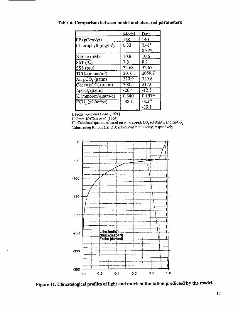
Table 6. Comparison between model and observed parameters
PP (gC/mVyr)
Chlorophyll (mg/m 3)
Nitrate (_tM)
SST (°C)
SSS (psu)
TCO 2 (mmol/m 3)
Air pCO 2 (_tatm)
Ocean pCOz (_tatm)
ApCO_ (_tatm)K (mmol/mV_tatm/d)'
FCO 2 (gC/m2/yr)
I. From Wong and Chan [1991]
II. From McClain et aI. [1996]
Model Data
168 140
0.33 0.411
0.32 _
10.8 10.6
7.8 8.2
32.68 32.67
2016.1 2059.7
320.9 329.8
300.5 317.0
-20.4 -12.8
0.340 0.137 m
-38.1 -8.3 m
-19.1
IT[. Calculated quantifies based on wind speed, CO 2solubility, and zSpCO 2.
Values using K from Liss & Merlivat and Wanninkhof, respectively.
-50
-100
-150
-200
-250
-300
-3500.0
}
T
i i _! |
....................._._.............i..............
r
; i i i" i, i =,
i i i---i : _ !......... _......... _......... ,...2 _,' ..... , ....,._......._ .............
.. ...........4............a . .
.... ........... ,t. ............ _._............. ]..
Li Felini_ldolted) [ _'!
.........................._ ........< ...... _.... _ ........._.......... _...........
• [ i __I
, i ' [ i !_]_ I
...... 1 _.2.........L ............. _.............._........--[---.-.--:-;............i
............. t-"....... _ .......... _ ........... "T'- .............. _...............i .... _
0.2 0.4 0.6 0.8 1.0
Figure 11. Climatological profiles of light and nutrient limitation predicted by the model.
17

Table 7. Comparison between 7 different model runs. All values were obtained by averaging the
model-data overlapping years (1973-1978), except for the last run (K from Wanninkhofand McGillis,
1999) where 21 years (1960-1980) were used for the averages. The first 2 spin-up years (1958-1959)
were eliminated from the averages
Run Type PP Chl-a NO 3 Ocean TCO 2 ApCO 2 K=KoO_
(gC/mVyr) (mg/m 3) (p.M) pCO 2(gatm_ (nm'lol/rn 3) (gatm) (mmoi/m 2/gatliffd)
0.340Baselinel
Baseline2
2xK o
4XKoNo iron
Abiotic
Ko(W_)
168
168
168
168
198
0
174
|ll, ml i
0.33 10.8 300.5 2016.1 -20.4
0.33 10.8 282.3 2005.4 -38.6
0.33 10.8 311.4 2022.5 -9.5
0.33 10.8 317.0 2025.0 -3.9
0.35 4.6 314.6 2023.8 -6.3
0 38.8 329.7 2028.3 7.7
0.33 10.8 318.6 2023.1 -2.3
0.156
0.679
1.358
FCO 2
(gC/mVyr)
-38.I
-29.6
1.358 -57.3
1.385 15.8
1.287 -45.6
18

1 I
SST (°C)
8
6 4_--- - •4 i i
SSS (psu)
I I
_.
8 NO3(ga)
4 = I
141210
33.0
32.8
32.6
16
12
216021202080204020001960
I I I I I I I I
I I I I I t I I
'_ _ _ T _ _ i,o 1,1
,,:f _ _ T _ _ 1,o 11
I t I I t I I t
o.6°"71 _ ? '_ _ _" -_ _ _ 1,o V 1l0.5 Chl-a (mg m -3) • •0.4 • A • • * _;__ • IL
0.2 I _ _ , J , t _ _ l _ ,
_ :P _ _ _ T _ _ 1,o 1,1I-CO= (llmol/kg) " • •
I I I I I I I I I I
360 I _ "? _ __'15 _ 17 I_ _) 110 111e_
340 pC02 (l_atm) 1l
320 • • • • - ,,,.e-'_ •
300280260 , i 0 , I _ i ,
440400360320280
:P f _ _ T _ _ 1,o 1,1 2
pC• 2 at 10°C (_atm) • •I I I I ' I l I I I
2 3 4 5 6 7 8 9 10 11 12Month
Figure 12. Model (solid line) versus observed (black circles and triangles) seasonal variability
of sea surface temperature and salinity, nitrate and chlorophyll averaged over the upper 80
meters, surface total carbon dioxide, pCO 2 at in situ temperature, and pCO 2 normalized to
10 °C. The gas exchange coefficient of Wanninkhof [1992] was used in this simulation.
19

The model pCO 2 is up to 40 gatm lower in the winter-spring months and about 20 gatm higher in
the summer. A significant improvement is achieved when the McGillis and Wanninkhof [ 1999] formu-
lation for K is used. Figure 13 shows the improved results. Note that the pCO 2 seasonal variability is
now much closer to the observed data. Figure 14 compares the model and observed pCO 2 interannual
variability for the period of 1973-1974. Predictions from run 1 (dotted line) and run 7 (solid line) are
shown together with the observed values (solid black circles). It is quite evident that more realistic
amplitude and phase of the seasonal cycle are achieved when the McGillis and Wanninkhof [1999]
formulation for K is used. Therefore we adopted this K formulation for our interannual run. The results
of the interannual run are discussed in the following sections.
5.0 SEASONAL VARIABILITY
Figures 15, 16, and 17 show the seasonal variability (from 1960-1980 monthly averages) of the
physical and biogeochemical model parameters. These are the vertical velocity, vertical eddy diffusivity,
temperature, photosynthetically available radiation (PAR), nitrate, ammonium, zooplankton, phytoplank-
ton, total carbon dioxide, oxygen, and iron. The vertical velocity is very weak in general (maximum of
3 crrgd) with upwelling peaks in the spring and fall when the wind cuff is largest. Maximum downwelling
occurs in December. The vertical advection effects are minimal when compared to vertical diffusion
(K). Maximum surface K values ranging from 900 to 1000 m2/d occur in late fall and winter. The
depth penetration of large K values follows the seasonal changes of the mixed layer depth; largest in
winter (120 m) and smallest in summer (20-40 m). Downwelling light intensity and penetration are
larger during April-August, peaking in May-June, The warmer temperatures are confined to the top 50
meters and the time period of May-October, with a peak in August-September. The seasonal variability
of phytoplankton, nitrate and iron are strongly correlated with top 50-meter peaks extending from May
through October. This is consistent with photosynthetic consumption of nutrients during the high growth
season. Total carbon dioxide and oxygen are strongly correlated with temperature due to the strong
dependence of solubility on temperature.
Oxygen anomalies relative to the temperature-determined saturation value (Figure 18) show that
there is a seasonal cycle of air-sea flux, with ingassing in winter and outgassing in summer. The oxygen
anomaly in the abiotic case is consistently less than in the full coupled model, suggesting that net
community production (Np) is positive at all times of the year. The biologically generated anomalies
contribute very little to the air-sea flux of oxygen. The difference between the biotic and abiotic cases
is greatest in summer, with a maximum of 3.3 gM in July, reflecting the seasonal cycle of Nj,. This
summer maximum in the NetCP was hypothesized by Wong and Chan [1991 ] to explain the absence of
a strong seasonal supersaturation ofpCO 2. The oxygen supersaturation in the summer months is 1.9-
2.8 times the value expected from thermal forcing alone. This is consistent with the oxygen supersatu-
rations determined by Emerson et al. [1993], which range from 1.4-2.6 times the values for argon (an
inert tracer of abiotic effects on oxygen), so rates of biological new production in the model are reason-
able and even on the high side.
20

141210
864
33.0
32.8
32.6
16
12
8
4
0.7
0.60.5
0.40.30.2
216021202080204020001960
36O340320300280
260
440400
360320280
I I
SST (oc)
IAv
I I
SSS (psu)
I I
l I I I I I I l
I I I I I I I !
4, _ _ T _ _ 1,o 11 1
II I I I ! _ 1 I
4, _ _ T _ _ 1,o 1,1 1
I I I I I I I I I I
_ ,4 ._ _ ( _ _ I,O 1,1 IA
Chl-a (mg m-3) • •
t • *----• = t,I I I I I I I I I I
_ 4, _ _ T _ _ 1,o 1,1 1
TCO 2 (gmol_g) _ • •
I I I I I I l I I I
_ _ _ _ T _ _ 1,o 1,1pCO 2 (gatm)
I I I I I I I I
A
J1
pCO 2 at 10°C (_atm)
I I I I I I I I
2 3 4 5 6 7 8 9Month
I I
i
10 11 12
Figure 13. As in Figure 12, except that the gas exchange coefficient of
Wanninkhofand McGillis [1999] was used in this simulation:
21

38O
Ocean pCO 2 in situ
I I I
360
E
00Q..
34O
32O
3OO
280
26O
240 _ , _ , ,
1973 1974 1975 1976 1977 1978 1979
Ocean pCO 2 at 10°C
,20t400
380
I I t I I
E 360
-t"-" 340
0_ 320
300
280
260
1973
I I t I I
1974 1975 1976 1977 1978 1979
Figure 14. Comparison between model and observed pCO 2 (in situ and normalized to 10 °C)
for the period of 1973-1978. Results from two model runs are shown: (1) the dotted line shows
the model results using the gas exchange formulation of Wanninkhof [1992];
(2) the solid line shows the model results using the gas exchange
formulation of Wanninkhofand McGiEis [1999]. The solid black
circles are the monthly averaged observed values.
22

0
5O
_-. 100E
"_" 150¢-
_- 200
a 250
300
350
0
..-.. IO0E
"" 150t-
200
13 250
_o.__
!w (crnct') -o
fill
Ill I
O. I _\\,
3OO
350
0
5O
.,-., 100E
"'" 150t"-
_- 200
a 250
3OO
35O
0
10
E-.....- 20t-Q..
30a
4O
50
Y D
5 5
4 4
T(°C)
2i__o_ _o
PAR (W m -2)
I I I t I i I I I I I
0 1 2 3 4 5 6 7 8 9 10 11 12
Time in Months
Figure 15. Seasonal variability of vertical velocity, vertical eddy diffusivity, temperature, and
downwelling irradiance simulated by the model.
23

0
5O
,,-.,, 100
E 150 "
" NOa(mmoi m -3) _ /_ 10 --...---__
_15 _" 15 ----------.---
" _ 20'
_- 200 20: _ 25 ---.-----.------ 25
250 -... 30 _ 30 .
300 -. - 35 _ 35 -
350 i 4n 40- :
50 o 1
150 .o5
D 250
3OO
350
0
5O
..--. 100E
150t"
Q.. 200
D 250
300
350
0
5O
..-.. 100E
150¢-
_- 200
250
30O
350
._15 /I 0_3 _..._____ \
o1_ -' o_°"
Zoo (mmoi N m -a)
I I I 1 1 I I
----'---..__j o,os_
I I 1 1
_
Phyto (mmol N m -3)I I I I 1 i I t 1 I I
0 1 2 3 4 5 6 7 8 9 10 11 12
Time in Months
Figure 16. Seasonal variability of nitrate, ammonium, zooplankton, and phytoplanktonconcentrations simulated by the model.
24

EV
..E:,.l..a
(Da
o
5o
lOO
15o
20o
25o
3oo
350
.:J T (°G )
o
5 5
4 4
50 TCO 2 (mmol m -3)
..-. 1oo _ 2030 _._,,.,,_.._
2040/ _ 2040
c, 200
250
300
350
2050
-2060
2070
2080
: 2090
-2050
2O60
2070
2080
2090
0
5O
100E
V
...E¢:)..
a
15o
2oo
25o
3oo
35o
_300--_._.
- -26028° _240_ 240 "---'-"-'----
-220 ., 220200 200180 180
Ev
t-
0 I_ I I I I I [ I I I
100160
1 50 160
200 t _------ 200 200
- 240 240
250 28o 280
300 320 320360 360
350 i i _ _ i t i t , I t0 1 2 3 4 5 6 7 8 9 10 11
Time in Months12
Figure 17. Seasonal variability of temperature, total carbon dioxide, oxygen, and iron
concentrations simulated by the model.
25

6.0 INTERANNUAL VARIABILITY
The interannual variability of the major parameters simulated by the model is illustrated in the
profile time series shown in Figures 19 and 20, and in the surface time series shown in Figure 21. The
temperature profile shows distinct warm and cold periods. Two warm periods occur on the series, one
during 1960-1965 and another during 1976-1980. The period during 1966-1975 exhibits colder (-1 °C)
temperatures in the top 150 meters. The oxygen profile series shows higher (-20 mmol/kg) concentra-
tions during the cold period due to increased solubility. The phytoplankton concentration in the upper
20 meters was higher (-0.1 mg/m 3) during the warmest temperature events (1961, 1963, and 1979).
0 2 Anomaly (O2-02 sat)
i ill I _ I I 1 ' !
I ' i :i . . I . i f _ !
6 _]___B,.at tc.i(s.olid)_ [ _-_ i !
_biotie (dotted) { , F i i/ I I ! / ',i I \ i _ !
4 ....... i I I -J- _I , [ ,
! I , l% i t _ ! I
____L_ i...... " i ....... _ !..;:,-"
. i i
"/ i , , i ...._...."_ / - .4 ............. i i t ! t I i i !
""=" i _ i I i i i/ i I _ _ i _ !/ I i i i ! iI i I i ,, i
-4 I i ....i I t i a I I i l
0 1 2 3 4 5 6 7 8 9 10 11 1
Months
Figure 18. Seasonal variability of surface oxygen anomaly predicted by the model.
Results from two runs are presented, an abiotic run (dotted line) and a biotic run (solid line).
The secular pCO 2 upward trend shown in the top tier of Figure 21 is manifested in the profile series of
total carbon dioxide concentration in Figure 19. The carbon dioxide increase of about 20 mmol/m 3 in
20 years, caused by the increased surface flux, is noticeable at depths of up to 250 meters. The highest
drawdown in the iron, nitrate, and carbon dioxide concentrations occurred during 1961-1963, a period
of warmest euphotic zone temperatures during which solubility was lowest and phytoplankton growth
was highest. Figure 22 shows the yearly and depth averaged (0-100 m) temperature and TCO 2 variabil-
ity, and the surface CO 2 flux and oceanic pCO 2 variability for the period of 1960-1980. The interannual
changes and trends are highlighted in this figure. Note the cooling trend in the temperature during the
1960s, followed by a warming trend during the mid to late 1970s. The air-sea CO 2 flux is always
negative, indicating that OWS P is a sink of atmospheric CO 2. The pCO 2 trends upward almost mono-
tonically showing an increase of about 30 l.tatm in 20 years. The TCO 2 follows the PC02 trend, show-
ing that the atmosphere and ocean are tightly coupled at OWS P.
26

0
50
.-. 100E
""" 150t-
O.. 200
D 250
300
350
0
50
100Ev 150...c:
200
a 250
300
35O
0
50
.-.. 100E
"-" 150(-.
t.-, 200O
O 250
3O0
350
0
5O
.-.. 100E
150t-
" 200
D 250
3OO
350
I1 , I , I I I I ....
T(°C)I | • I I I I I I [ 1 I I I I I
0_0_1_011_1_ I io 0
KvI I t I I t I I 1 I I I I I I
201 I I I I I I I I I l I l I I I I
i _ i i J 'o_'' 'llli ' -'-_11.' '_lo ' '
I I I I I I I I I t I I I I I 1 l I I I
60 62 64 66 68 70 72 74 76 78 80
YEAR
Figure 19. Interannual variability of temperature, vertical eddy diffusivity, total carbon
dioxide, and oxygen simulated by the model.
27

350 i , _ , J t , , _ _ _ , _ , I
0 I l I I I I I I I 1 ,,
2oo_2_._oo
300
350
0 ! I I T t 1 I I I | 1 I 115 I I I I .I I I I
350
,,E 150
.- 200250
300 NH 4 (gM)
350 , _ , _ , , t , , _ , _ r' i _ _ , _ ,60 62 64 66 68 70 72 74 76 78 80
YEAR
..-... 100E
"-" 150
200
250
.-. 100E
150t--
200O
250
100E
150t-
_- 200O
250
Figure 20. Interannual variability of phytoplankton, iron, nitrate, and ammonium
simulated by the model.
28

I I I I [ I I I I 1 I I I t I I t I I I
440 Air(solid), I
400 Ocean(dashed)'lOOC(dotted) __j A._, _t t'!,_tl i / ,' _; ", ', .'i t_r[{t .,it _! !t
260 ;__ V"_( V-_ }" v v, !:, ,., _r-_ v v v v1
240 I
, , , , , , , , , I , , , , , , , , , ,
' ' ' ' ' ' ' ' ' 'A'_' A'A'A'A'A'A' ' ' '_MLD(solid), SST(dotted) 1i_ /I. _l ,I >, li , 14
,_ 120 A l_ li II _ /i .h it _,N ,l 't 't, " 'i " ', .,I ,_ tl .ii 12 ...II' I tI ,t1 ,, ,'i "1 ]' ,_ i. , i / , i tl/ ttl_l ll li'_l ,_ l, ,,il I I f _ !i i It
,) t_,A_,l,l,t,_,I_l,ttl,/l'/:l//:i:,,l-_- 4
,o_JVtTVVVVt/'/', , , , , , , , , , , 20 I I I I I I I I I I I I t t t I I I 1 I
2060 - - - - z --I'rck2(ioliii,oi-(dltte_) i i
2040.,_i_ ,_,_,__ _/1 _ / 320
° o olVVVVVVVVV0 1980
1960 , _ _ _ i , i i lI , i i , i t i i i : ; ; ; ili ; i, il ; : 240
200 ] Fe(solid), NH4(dashed) t 0.5180t, ` NOa/50(dotted) 0.4_..-.. 160
80 _ 0.1 Z
60 0.0
60 62 64 66 68 70 72 74 76 78 80
YEAR
Figure 21. Time series of simulated atmospheric pC02, oceanpCO 2, SST, mixed layer depth,
total carbon dioxide, oxygen, iron, nitrate, and ammonium.
29

7.0 CARBON FLUX BUDGET
Figure 23 represents the climatological (1960-1980) ecosystem carbon flux balance. The main
compartments in this flow chart are the phytoplankton, zooplankton, respired DOC, and total CO 2
carbon stocks. The numbers indicate the carbon flux between ecosystem components in gC/m2/yr. The
ammonium and nitrate boxes were replaced by the net community production (76 gC/m2/yr), which
represents all sources and sinks of macronutrients combined (equation 14). Note that the air-sea (44
gC/mVyr) and bottom (23 gC/m2/yr) carbon fluxes are balanced by the POC+DOC export (60 gC/mV
yr) and fecal pellet loss (7 gC/m2/yr) through the bottom. The total gross production (uptake) is 174 gC/
m2/yr. Therefore, the total carbon required for photosynthesis is partitioned among the following sources:
44% (76 gC/m2/yr) originates from the TCO 2 pool - of these 44%, 5% comes from DOC respiration,
13% comes from the bottom flux, and 25% from the atmosphere (air-sea flux). The other 56% (98 gC/
m2/yr) of the required equivalent carbon comes from the recycling of zooplankton and phytoplankton
losses (death, respiration, and fecal pellet production).
8.0 SUMMARY AND CONCLUSIONS
A coupled ecosystem/carbon flux model was developed, validated, and used to simulate bio-
geochemical parameters at OWS P. A series of sensitivity runs revealed that the most significant
improvement in the simulation of the surfacepCO 2 is obtained by the use of a recently developed cubic
formulation for the gas exchange coefficient (Wanninkhofand McGillis, 1999). This result shows that
the ocean and atmosphere are much more closely coupled at high (> 10 m/s) wind speeds than indi-
cated by the previous wind-dependent formulations (Liss and Merlivat, 1986; Tans et al., 1990;
Wanninkhof, 1992).
All biogeochemical parameters, when averaged over the period of available concurrent observa-
tions (1973-1978), are within less than 5% of the observed values. The only exception is the sea-air
CO 2 flux which departs more significantly from previously reported values. We attribute this differ-
ence to the elusive nature of sea-air CO 2 estimates in the ocean and the variety of formulations used in
the literature to derive the gas exchange coefficient. For example, our lowest CO 2 flux estimate is -29.6
gC/m2/yr when we use the Liss and Merlivat [ 1986] gas exchange formulation. Wong and Chan [1991 ],
also using the Liss and Merlivat [ 1986] gas exchange formulation, report a value of -8.4 g C/m2/yr. Our
CO 2 flux value is even higher (-45.6 gC/m2/yr) when we use the Wanninkhofand McGillis [1999] gas
exchange formulation. However, the model estimates for the surface flux and those derived from ApCO 2
measurements are not entirely equivalent because the model provides a dynamically coupled flux esti-
mate, whereas the air-sea flux estimates from observed ApCO 2 are obtained from a relatively small
number of discrete data points. Therefore, global estimates of air-sea CO 2 flux derived using air-sea
flux models to extrapolate from observed pCO 2 may not be realistic. In the short term, fully prognostic
models may give the best estimates provided that they achieve sufficient agreement with other observ-
able quantities such as temperature, chlorophyll, and TCO 2.
3O
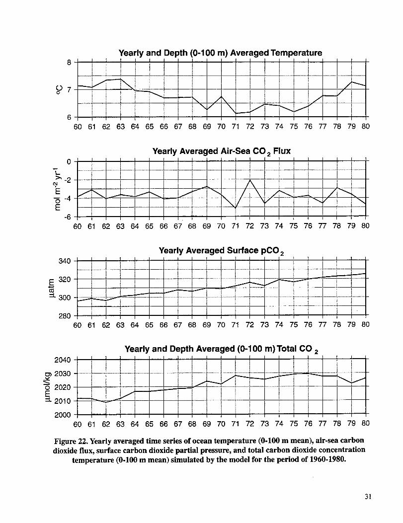
_
_
I
i!I
Yearly and Depth (0-100 m) Averaged TemperatureI I
B
tt !
I I
t ti it !
I i i 1 ! i t i ._i
I i.........i ,
J I
60 61 62 63 6'4 65 66 67 68 69 70 71 72 73 74 75 76 77 78 79 80
0
>'-2
E-6-4E
-6
Iii
! ii i .,
Yearly Averaged Air-Sea CO 2 Fluxi j , t i i I E ! i i I i
.............................. i ............................. ,
i I I 1 _I
Z
I ,i
i
i
!
t
60 61 62 63 64 65 66 67 68 69 70 71 72 73 74 75 76 77 78 79 80
340
E 32Ot_
:=L 300
280
Yearly Averaged Surface pCO 2J I I I ; I I I " I I I l 1 1 I I I! i i __ i __ ' ................1.......'....l...............1...............L_j .........l.....L__L_
........,..........l....... 7--7 .............. i ..............i ........ T l T.... i i / L_.--L I I ! ! I .... / / !_ _ t
i I , ! I i
I i I i I I ' tt i i i I_ ' _ i _ _ •i, l i _ ' I i t i i I I
60 61 62 63 64 65 66 67 68 69 70 71 72 73 74 75 76 77 78 79 80
2040
2030 ............
o 2020
_2010 _
2000 i
Yearly and Depth Averaged (0-100 m)Total CO 2
ii ,i i..........--_----e ..................................."
}
i I , I
! ,• i
60 61 62 63 64 65 66 67 68 69 70 71 72 73 74 75 76 77 78 79 80
Figure 22. Yearly averaged time series of ocean temperature (0-100 m mean), air-sea carbon
dioxide flux, surface carbon dioxide partial pressure, and total carbon dioxide concentration
temperature (0.100 m mean) simulated by the model for the period of 1960-1980.
31
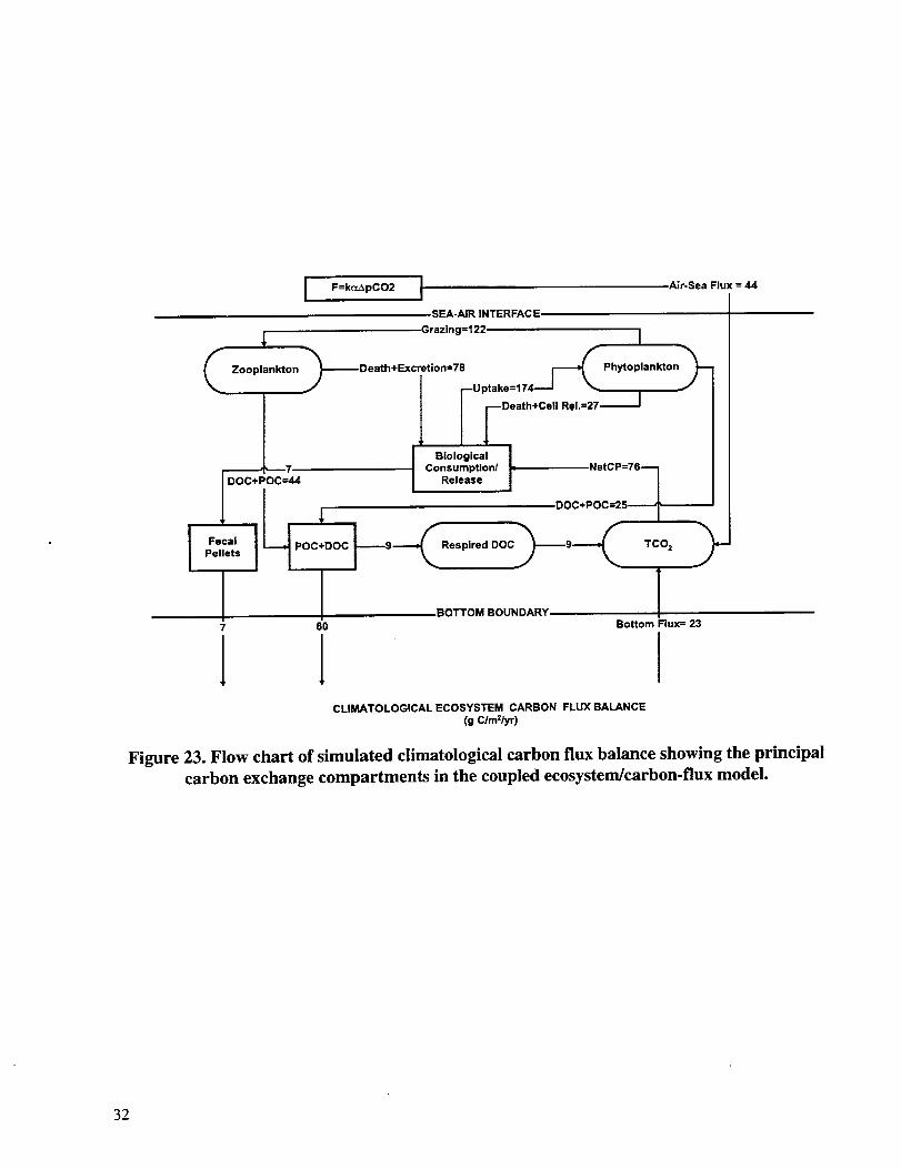
F=k_pCO2 I Air-Sea Flux = 44
SEA-AIR INTERFACE
_, Grazing=122 ' ' [
,IfBiological
7 Consumption/
J h DOC+POC=25--'--T_pF_/_l s POC+DOC J-_----9_ Respired DOC _9_
7 60
BOTTOM BOUNDARY
TCO z
1Bottom Flux= 23
CLIMATOLOGICAL ECOSYSTEM CARBON FLUX BALANCE
(g C/mZlyr)
Figure 23. Flow chart of simulated climatological carbon flux balance showing the principal
carbon exchange compartments in the coupled ecosystem/carbon-flux model.
32

REFERENCES
AndriC C., C. Oudot, C. Genthon, and L. Merlivat, CO 2 fluxes in the tropical Atlantic during FO-
CAL cruises, J. Geophys. Res., 91, 11,741-11,755, 1986.
Antoine, D., and A. Morel, Modelling the seasonal course of the upper ocean pC02: (I). Develop-
ment of a one-dimensional model, Tellus, 47B, 103-121, 1995.
Antoine, D., and A. Morel, Modelling the seasonal course of the upper ocean pC02:(II). Validation
of the model and sensitivity studies, TelIus, 47B, 122-144, 1995.
Archer, D., S. Emerson, T. Powell, and C. S. Wong, Numerical hindcasting of sea surface pCO 2 at
Weathership OWS P, Prog. Oceanogr., 32, 319-351, 1993.
Batrakov, G. F., A. A. Bezborodov, V. N. Yeremeyev, and A. D. Zemlyanoy, CO 2 exchange between
Indian Ocean waters and the atmosphere, Oceanology, 21, 39-43, 1981.
Boyd, P. W., D. L. Muggli, D. E. Varela, R. H. Goldblatt, R. Chretien, K. J. Orians, and P. J.
Harrison, In vitro iron enrichment experiments in the NE subarctic Pacific, Mar. Ecology Progr.
Ser., 136, 179-193, 1996.
Broecker, W. S., and T.-H. Peng, The vertical distribution of radon in the BOMEX area, Earth
Planet. Sci. Lett., 11, 99-108, 1971.
Broecker, W. S., and T.-H. Peng, Gas exchange rates between air and sea, Tellus, 26, 21-35, 1974.
Conkright, M., S. Levitus, and T. Boyer, NOAA Atlas NESDIS 1, World Ocean Atlas 1994, U. S.
Dep. of Comm., Washington D. C., 1994.
Dobson, F. W., and S. D. Smith, Bulk models of solar radiation at sea, Q. J. R. Meteorol. Soc., 114,
165-182, 1988.
Duce, R. A., Sources, distributions, and fluxes of mineral aerosols and their relationship to climate,
in Aerosol Forcing of Climate, R. J. Charlson and J. Heintzenberg, editors, John Wiley and Sons,
43-72, 1995.
Frost, B. W., A modelling study of processes regulating plankton standing stock and production in
the open subarctic Pacific Ocean, Prog. Oceanogr., 32, 17-56, 1993.
Fushimi, K., Variation of carbon dioxide partial pressure in the western North Pacific surface water
during the 1982-1983 El Nifio event, Tellus, Ser. B, 39, 214-227, 1987.
Emerson, S., P. Quay, and P. A. Wheeler, Biological productivity determined from oxygen mass
balance and incubation experiments, Deep Sea Res., 40, 2351-2358, 1993.
Goyet, C., and A. Poisson, New determination of carbonic acid dissociation constants in sea water as
a function of temperature and salinity, Deep Sea Res., 36, 1635-1654, 1989.
33
Gordon,L. I., P.K. Park,S.W. Hager,andT.R. Parsons,Carbondioxidepartialpressuresin northPacific surfacewaters- timevariations,J. Oceanogr. Soc. Japan, 27, 81-90, 1971.
Gordon, L. I., R K. Park, J. J. Kelley, and D. W. Hood, Carbon dioxide partial pressures in north
Pacific surface waters, 2. General late summer distributions, Mar. Chem., 1, 191-198, 1973.
Inoue, H., Y. Sugimura, and K. Fushimi, pC02 and 5_3C in the air and surface sea water in the
western North Pacific, Tellus 39 B, 228-242, 1987.
Inoue, H., and Y. Sugimura, Distributions and variations of oceanic carbon dioxide in the western
North Pacific, eastern Indian, Southern Ocean south of Australia, Tellus 40 B, 308-320, 1988.
Keeling, C. D., Carbon dioxide in surface ocean waters, 4, Global distribution, J. Geophys. Res., 73,
4543-4554, 1968.
Liss, P. S., Tracers of air-sea gas exchange, Phil. Trans. R. Soc. Lond., A 325, 93-103, 1988.
Liss, R S., and L. Merlivat, Air-sea exchange rates: Introduction and synthesis. In: The Role of Air-
Sea Exchange in Geochemical Cycling, R Buat-M6nard, editor, NATO ASI Series C: Mathemati-
cal and Physical Sciences, Vol. 185, pp. 113-128, 1986.
Maldonado, M. T., R W. Boyd, R J. Harrison, and N. M. Price, Co-limitation of phytoplankton
growth by light and Fe during winter in the NE subarctic Pacific Ocean, Deep-Sea Res. II, 46,
2475-2485, 1999.
Martin, J. H., S. E. Fitzwater, W. W. Broenkow, VERTEX: phytoplankton/iron studies in the Gulf of
Alaska, Deep-Sea Res., 36, 645-680, 1989.
McClain, C. R., K. Arrigo, K.-S. Tai, and D. Turk, Observations and simulations of physical and
biological processes at ocean weather Station P, 1951-1980, J. Geophys. Res., 101, 3697-3713,
1996.
McClain, C. R., S. R. Signorini, K.-S. Tai, K. Arrigo, and R. Murtugudde, An ecosystem model for
the simulation of physical and biological oceanic processes - IDAPAK User's guide and applica-
tions, NASA/TM-1998-206856, NASA Goddard Space Flight Center, Greenbelt, Maryland, April
1998.
Millero, F. J., K. Lee, and M. Roache, Distribution of alkalinity in the surface waters of the major
oceans, Mar. Chem., 60, 111-130, 1998.
Murphy, R R, D. E. Harrison, R. A. Feely, T. Takahashi, R. E Weiss, and R. H. Gammon, Variability
of zipCO 2 in the subarctic North Pacific. A comparison of results from four expeditions, Tellus,
50B, 185-204, 1998.
Oudot, C., and C. Andri6, Variabilit6 des pressions partielles de CO 2 oc6anique et atmosph6rique
dans l'Atlantique tropical, Oceanol. Acta 9, 169-177, 1986.
34

Oudot,C., andC. Andri6,Short-termchangesin thepartialpressureof CO 2 in eastern tropical
Atlantic surface seawater and in atmospheric CO 2 mole fraction, Tellus 41 B, 537-553, 1989.
Oudot, C., and C. Andri6, and Y. Montel, Evolution du CO 2 oc6anique et atmosph6rique sur la
p6riode 1982-1984 dans l'Atlantique tropical, Deep-Sea Res., 34, 1107-1137, 1987.
Peng, T.-H., T. Takahashi, and W. S. Broecker, Surface radon measurements in the North Pacific
Ocean OWS P, J. Geophys. Res., 79, 1772-1780, 1974.
Peng, T.-H., W. S. Broecker, G. C. Mathiew, and Y.-H. Li, Radon evasion rates in the Atlantic and
Pacific Oceans as determined during the Geosecs program, J. Geophys. Res., 84, 2471-2486,
1979.
Pond, S., and G. L. Pickard, Introductory Dynamic Oceanography, 241 pp., Pergamon, Tarrytown,
N. Y., 1978.
Smethie, W. M., Jr., T. Takahashi, D. W. Chipman, and J. R. Ledwell, Gas exchange flux in tropical
Atlantic Ocean determined from 2Z2Rn and pCO 2, J. Geophys. Res., 90, 7005-7022, 1985.
Sundquist, E. T., Geological perspectives on carbon dioxide and carbon cycle, in The Carbon Cycle
and Atmospheric C02: Natural Variations Archean to present, Geophys. Monogr. Ser., vol. 32,
edited by E. T. Sundquist and W. S. Broecker, pp 5-59, AGU, Washington, D. C., 1985.
Takahashi, T., D. Chipman, and T. Volk, Geographical, seasonal, and secular variations of the partial
pressure of CO 2 in surface waters of the North Atlantic TTO program, in Carbon Dioxide, Science
and Consensus (CONF-820970), Institute for Energy Analysis, Oak Ridge Associated Universi-
ties, Washington, D. C., 123-145, 1983.
Takahashi, T., J. Olafsson, J. G. Goddard, D. W. Chipman, and S. C. Sutherland, Seasonal variations
of CO 2 and nutrients in the high-latitude surface oceans: A comparative study, Global
Biogeochem. Cycles, 7, 843-878, 1993.
Takahashi, T., R. A. Feely, R. E Weiss, R. H. Wanninkhof, D. W. Chipman, S. C. Suthedand, and T.
T. Takahashi, Global air-sea flux of CO2: An estimate based on measurements of sea-air pCO 2
difference, Proc. Natl. Acad. Sci., vol. 94, pp. 8292-8299, 1997.
Taylor, A. H., A. J. Watson, M. Ainsworth, J. E. Robertson, and D. R. Turner, A modeling investiga-
tion of the role of phytoplankton in the balance of carbon at the surface of the North Atlantic,
Global Biogeochem. Cycles, 5, 151-171, 1991.
Tegen, I., and I. Fung, Modeling of mineral dust in the atmosphere: Sources, transport, and optical
thickness, J. Geophys. Res., 99, 22,897-22,914, 1994.
Weiss, R. E, The solubility of nitrogen, oxygen and argon in water and seawater, Deep Sea Res., 17,
721-735, 1970.
Weiss, R. E, Carbon dioxide in water and seawater: The solubility of a non-ideal gas, Mar. Chem., 2,
203-215, 1974.
35

Wanninkhof,R., andW.R. McGillis, A cubicrelationshipbetweenair-seaexchangeandwind speed,Geophys. Res. Lett., 26, 1889-1892, 1999.
Wanninkhof, R., Relationship between wind speed and gas exchange over the ocean, J. Geophys.
Res., 97, 7373-7382, 1992.
Wong, C. S., and Y.-H. Chan, Temporal variations in the partial pressure and flux of CO 2 at ocean
Station P in the subarctic northeast Pacific Ocean, Tellus, 43B, 206-223, 1991.
36


I Form ApprovedREPORT DOCUMENTATION PAGE OMBNo.0704-0188
Publi_ 'reportingburden for this collection of informationis estimated to average 1 hour per response, includingthe time for reviewinginstructions, searchingexistingdata sources,gathering and maintaining the data needed, and completing and reviewingthe collection of information. Send comments regarding this burden estimate or any other aspect of thiscollectionof information, including suggestionsfor reducing thisburden, to WashingtonHeadquarters Services, Directorate for Information Operations and Reports, 1215 JeffersonDavis Highway, Suite 1204, Arlington, VA 22202-4302, and to the Office of Management and Budget, Paperwork Reduction Project (0704-0188), Washington, OC 20503,
1. AGENCY USE ONLY (LeavebIank) 1_2_Rg_%ToDATE I 3"REP--OR_FTyPE_NDOATE_COVERED'IeChnlCa_J-_]bllCat]on
4. TITLE AND SUBTITLE 5. FUNDING NUMBERS
One-Dimensional Coupled Ecosystem-Carbon Flux Model for the
Simulation of BiogeochemicaI Parameters at Ocean Weather Station P 970.2
I
6. _UTHOR(S)..>. _lgnonm, C. McClain, J. Christian, C.S. Wong
7. PERFORMING ORGANIZATION NAME(S)'AND ADDRESS (ES)
Goddard Space Flight Center
Greenbelt, Maryland 20771
9. SPONSORING / MONITORING AGENCY NAME(S) AND ADDRESS (ES)
National Aeronautics and Space Administration
Washington, DC 20546-0001
8. PEFORMING ORGANIZATION
REPORT NUMBER
2000-01898-0
10. SPONSORING/MONITORING
AGENCY REPORTNUMBER
TP--2000-209892
15. NUMBER OF PAGES
3616. PRICE CODE
11 ._SU_PPLEMENTARY. N_T_S -_. _lgnonm; SAIC General Sciences Corporation; Beltsville, Maryland
J. Christian; Universities Space Research Assoc.; NASA/GSFC; Greenbelt, Maryland
C.S. Won_; Centre for Ocean Climatic Chemistry; Ins.titute of Ocean Studies; Sidney,, British Columbia ,i2a. DISTRIBUTION/AVAILABILITY STATEMENT 12b. DISTRIBUTION CODE
Unclassified-Unlimited
Subject Category: 42
Report available from the NASA Center for AeroSpace Information,
7121 Standard Drive, Hanover, MD 21076-1320. (301) 621-0390.m m[H[mI[
13. ABSTRACT (Maximum 200 words)
In this Technical Publication, we describe the model functionality and analyze its application to the
seasonal and interannual variations of phytoplankton, nutrients, pCO 2 and CO 2concentrations in the
eastern subarctic Pacific at Ocean Weather Station P (OWSP, 50 °N 145 °W). We use a verified one-
dimensional ecosystem model (McClain et al., 1996), coupled with newly incorporated carbon flux
and carbon chemistry components, to simulate 22 years (1958-1980) of pCO 2 and CO 2variability at
Ocean Weather Station P (OWS P). This relatively long period of simulation verifies and extends the
findings of previous studies (Wong and Chan, 1991; Archer et al., 1993; Antoine and Morel, 1995a;
Antoine and Morel, 1995b) using an explicit approach for the biological component and realistic
coupling with the carbon flux dynamics. The slow currents and the horizontally homogeneous oceanin the subarctic Pacific make OWS P one of the best available candidates for modeling the chemistry
of the upper ocean in one dimension. The chlorophyll and ocean currents composite for 1998 shown in
Figure 1 illustrates this premise. The chlorophyll concentration map was derived from SeaWiFS data
and the currents are from an OGCM simulation (from R. Murtugudde)....... iiiii I II
lrrr
14. SUBJECT TERMS
ecosystem dynamics, biogeochemistry, carbon flux
17. SECU RITY CLASSIFICATIONOF REPORT
Unclassified 18.SEC"R CGESlnCATIONIOF THIS PAGE
Unclassified
NSN 7540-01-280-5500
19. SECURITY CLASSIRCATION 28. LIMITATION OF ABSTRAC]
OF ABSTRACT
Unclassified UL
Standard Form 298 (Rev. 2-89)


![Impacts of atmospheric variability on a coupled upper-ocean//ecosystem …web.uvic.ca/~monahana/monahan_denman.pdf · 2004-06-16 · ocean/ecosystem model. [5] Section 2 of this paper](https://img.dokumen.tips/doc/110x75/5fa028888b7f711ce374a0ec/impacts-of-atmospheric-variability-on-a-coupled-upper-oceanecosystem-webuviccamonahanamonahan.jpg)


