Embed Size (px)
Citation preview

ON THE VALIDITY OF THE WAGNER HYPOTHESIS IN THIN-WALLED OPEN- PROFILE MEMBERS
by
Monica Kaeline Falgoust
BS in Civil Engineering, University of Pittsburgh, 2002
Submitted to the Graduate Faculty of
School of Engineering in partial fulfillment
of the requirements for the degree of
Master of Science in Civil Engineering
University of Pittsburgh
2004

UNIVERSITY OF PITTSBURGH
SCHOOL OF ENGINEERING
This thesis was presented
by
Monica Kaeline Falgoust
It was defended on
December 3, 2004
and approved by
Dr. Kent A. Harries, Assistant Professor, Department of Civil and Environmental Engineering
Dr. Jeen-Shang Lin, Associate Professor, Department of Civil and Environmental Engineering
Dr. John F. Oyler, Adjunct Professor, Department of Civil and Environmental Engineering
Dr. Christopher J. Earls, Chairman and Associate Professor, Department of Civil and Environmental Engineering
Thesis Director
ii

ON THE VALIDITY OF THE WAGNER HYPOTHESIS FOR THIN-WALLED OPEN-PROFILE MEMBERS
Monica K. Falgoust, MS
University of Pittsburgh, 2004
The Wagner Hypothesis states that when a thin-walled open-profile member is subjected
to an axial loading leading to global instability, the longitudinal stresses developing within the
fibers composing the cross-section become inclined to the normal plane; thus taking on a helical
shape with respect to the longitudinal axis of the member. It is assumed that the longitudinal
fiber stresses act as “follower-forces” and thus assume the same inclination as the cross-sectional
fibers and thus produce a torsional moment about the longitudinal axis of the member. Classical
second-order theories for calculating critical buckling loads based on the line of shear centers for
thin-walled open-profile members have been developed by Timoshenko and Vlasov, which
include the use of the Wagner effect. However, a competing theory has been developed by
Ojalvo that utilizes the line of cross-sectional centroids (rather than cross-sectional shear centers)
as a reference axis while at the same time rejecting the use of the Wagner Hypothesis. Ojalvo
proposes that the Wagner Hypothesis violates common statical principles as well as is deficient
for not identifying the free body with which torsional equilibrium is expressed.
The current study explored the validity of the second-order theories using nonlinear finite
element techniques to produce critical buckling loads for various thin-walled open-profile
members. Critical buckling loads obtained from this analysis were compared with numerical
results provided by each theory as well as experimental results. Not only did the present
research evaluate the behavior of various torsional members at their critical buckling loads, but it
iii

also explored the notion that the principal stresses take on a helical shape once torsion has
occurred (i.e. the stresses do indeed behave as “follower-forces”) using graphical representations
of the members created within the finite element software. Conclusions were made based on the
comparison of finite element results compared with theoretical results and experimental tests.
The current study found that the Wagner Hypothesis is valid due to positive agreement between
finite element results, numerical solutions, and experimental tests. Recommendations were made
concerning the possibility of further research regarding this topic.
iv

TABLE OF CONTENTS
1.0 INTRODUCTION .............................................................................................................. 1
1.1 LITERATURE REVIEW ............................................................................................... 4
1.2 OVERVIEW OF THESIS ORGANIZATION ............................................................. 24
2.0 FINITE ELEMENT METHOD ........................................................................................ 26
2.1 FINITE ELEMENT ANALYSIS PROCEDURE......................................................... 27
2.2 NONLINEAR FINITE ELEMENT ANALYSIS ......................................................... 28
2.2.1 Nonlinear Equilibrium Solution Methods............................................................. 30
2.3 ELEMENT TYPE......................................................................................................... 30
2.4 FINITE ELEMENT MESH .......................................................................................... 32
2.5 IMPERFECTION SEED .............................................................................................. 33
2.6 MATERIAL PROPERTY DEFINITIONS................................................................... 34
3.0 VERIFICATION STUDY ................................................................................................ 35
3.1 VERIFICATION STUDY RESULTS.......................................................................... 35
4.0 FINITE ELEMENT MODELS......................................................................................... 42
4.1 DOUBLY SYMMETRIC W-SECTION LOADED BY UNIFORM MOMENT........ 43
4.2 FLANGED CRUCIFORM COLUMN LOADED BY AXIAL FORCE...................... 46
4.3 TEE COLUMN LOADED BY ECCENTRIC AXIAL COMPRESSIVE FORCE...... 59
5.0 CONCLUSIONS AND RECOMMENDATIONS ........................................................... 73
APPENDIX A............................................................................................................................... 76
ELEVATION VIEWS OF COLUMN SECTIONS.................................................................. 76
APPENDIX A1......................................................................................................................... 77
v

APPENDIX A2......................................................................................................................... 78
APPENDIX B ............................................................................................................................... 80
ABAQUS INPUT FILES.......................................................................................................... 80
APPENDIX B1 ......................................................................................................................... 82
APPENDIX B2 ......................................................................................................................... 86
APPENDIX B3 ......................................................................................................................... 89
APPENDIX B4 ......................................................................................................................... 92
APPENDIX B5 ......................................................................................................................... 99
APPENDIX B6 ....................................................................................................................... 106
APPENDIX B7 ....................................................................................................................... 109
APPENDIX C ............................................................................................................................. 113
THEORETICAL RESULTS................................................................................................... 113
APPENDIX C1 ....................................................................................................................... 114
APPENDIX C2 ....................................................................................................................... 115
APPENDIX C3 ....................................................................................................................... 117
APPENDIX D............................................................................................................................. 120
PRINCIPAL STRESS CALCULATIONS............................................................................. 120
APPENDIX D1....................................................................................................................... 121
APPENDIX D2....................................................................................................................... 125
BIBLIOGRAPHY....................................................................................................................... 127
vi

LIST OF TABLES Table 1: Inclination of Principal Plane (Cruciform) ................................................................... 121
Table 2: Inclination of Principal Plane (Tee).............................................................................. 125
vii

LIST OF FIGURES
Figure 1: Translation and Rotation of Elastic Cross-Sectional Slice. (Galambos 1968)................ 7
Figure 2: Twist Due to Differential Warping of Two Adjacent Cross-sections. (Galambos 1968)8
Figure 3: Postbuckling of Perfect Column. (a) Stable (b) Unstable Curve. (Galambos 1998).... 12
Figure 4: Postbuckling Curves for Initially Imperfect Systems. (Galambos 1998)...................... 13
Figure 5: Cruciform Behaving as Tee Under Torsional Loading. (Ojalvo 1990) ........................ 21
Figure 6: S4R Element.................................................................................................................. 32
Figure 7: W12x50 Cross-section .................................................................................................. 36
Figure 8: Deformed Shape of a Simply Supported Beam under Eccentric Loading .................... 38
Figure 9: Variation of Angle of Twist and Derivatives Along Beam Length. (Galambos 1968). 39
Figure 10: Rotation about Longitudinal Axis of W-Section Compared to Galambos’ Plot......... 40
Figure 11: Cruciform Column Cross-sectional Dimensions......................................................... 47
Figure 12: Load vs. Rotation for Section having t = 0.1 .............................................................. 50
Figure 13: Mode 1 Deflected Shape of Cruciform Column Exhibiting Local Buckles................ 51
Figure 14: Mode 1 Buckled Shape of Cruciform Column with 0.25" Thickness......................... 52
Figure 15: Postbuckled Shape of Cruciform Column with Scale Factor of L/1000..................... 53
Figure 16: LPF vs. Rotation about Longitudinal Axis for Web Intersection at Mid-height......... 54
Figure 17: Maximum Principal Angle on Upper Half of Flange on Cruciform-Shaped Column 56
Figure 18: Principal Angle and Rotation about Z-Axis along Length of Cruciform.................... 58
Figure 19: a) Negative Eccentricity b) Positive Eccentricity........................................................ 60
Figure 20: Metric Dimensions of Tee Cross-section .................................................................... 61
Figure 21: English Dimensions of Tee Cross-section................................................................... 63
viii

Figure 22: Mode 1 Buckled Shape of Tee Model at Scale Factor L/1000 ................................... 65
Figure 23: Postbuckled Shape of Tee Model at L/1000 ............................................................... 66
Figure 24: Load vs. Rotation for Tee Section for Various Scale Factors ..................................... 67
Figure 25: Maximum Principal Angles on Tee Flange Section.................................................... 70
Figure 26: Principal Angles and Rotation about Z-Axis along Flange Length (1/4 of Pcr)........ 71
Figure 27: Elevation of Cruciform Model .................................................................................... 77
Figure 28: Elevation of Tee Model with Metric Dimensions ....................................................... 78
Figure 29: Elevation of Tee Model with English Dimensions ..................................................... 79
ix

NOTATION
a Distance between a point on the cross section and the shear center
Bx, By Bending Stiffness about the x and y axis
CT St. Venant Torsional Stiffness
CW Warping Stiffness
E Modulus of Elasticity
e(Ojalvo) ey - yo
ey Eccentricity
G Shear Modulus
Ix, Iy Moment of Inertia about x and y axis
Iω Warping Moment of Inertia
KT St. Venant Torsion Constant
k(Ojalvo) π/L
L Length of Member
m(Ojalvo) Couples
n Energy State
ro Radius of Gyration
T(Ojalvo) Internal Moment
V Shear Force
u, v Displacements
x, y Coordinates of any point on a cross section
xo, yo Coordinates of the Shear Center
x

βx Cross Sectional Constant Defined by Eqn. 1-3
φ Angle of Twist
xi

ACKNOWLEDGEMENTS I would like to thank my thesis advisor, Dr. Christopher Earls, for providing me with guidance,
insight, and his vast wisdom throughout my academic pursuits.
I would like to thank my family for their unending love and support; without their faith in me,
none of my dreams would be possible.
I would like to thank all of my friends, and especially those who resided on the 11th floor of
Benedum hall; sharing fun experiences with you allowed me to stay balanced throughout my
academic career.
I would like to thank Muharrem Aktas, Brandon Chavel, and Brian Kozy; their engineering
understanding has been an enormous aid in the completion of this project.
Last but certainly not least, I would like to thank my best friend, Jason O’Neil, for reminding me
to laugh, since that is one of the most important things in life.
xii

1.0 INTRODUCTION
The Wagner Hypothesis provides that when a thin-walled open-profile member is subjected to an
axial loading leading to global instability, the longitudinal stresses developing within the fibers
composing the cross-section become inclined to the normal plane and thus produce a torsional
moment about the longitudinal axis of the member. This theory relies on the assumption that a
bar is comprised of a bundle of filaments that act somewhat independently of one another; a
useful analog is a cross-section composed of bundle of straws. Before the bar becomes unstable
and begins to twist, the filaments have a compressive stress in them due to the axial loading.
Once the member begins to twist due to the activation of some global instability mode, the
filaments are no longer parallel to the longitudinal axis of the member. It is assumed that the
longitudinal fiber stresses act as “follower forces” and thus assume the same inclination as the
cross-sectional fibers. These inclined stresses then create a torsional moment about the
longitudinal axis as well as an axial force resultant (Goodier 1950). It is assumed that as the
section twists the stresses will begin to form a helical shape around a longitudinal axis formed by
the line of shear centers of all cross-sections occurring along the member length; this helix,
therefore, will follow the geometry of the deformed shape. The timeline under which the
hypothesis evolved began with the classical theory for lateral-torsional buckling of thin-walled
open-profile bars developed by Michell (1899) and Prandtl (1899). It was then extended further
by Timoshenko (1905) to I-shaped bars with two axes of symmetry in the same plane. Wagner
(1929) then applied these principles to the case of the shear center of thin-walled open-profile
bars of arbitrary cross-section. The classical theories based on the assumptions that Wagner
made have endured.
1

Second-order theories have been further developed based on the work of Timoshenko and
Wagner, more recently by Galambos (1968). These theories apply to various thin-walled open-
profile sections that are subjected to various loadings which cause some form of torsional failure.
Also recently, a competing theory has been developed by Ojalvo (1990), which is not based on
the shear center as the torsional axis and does not accept the Wagner Hypothesis. Ojalvo
proposes that the Wagner Hypothesis violates common statical principles as well as is deficient
for not identifying the free body with which torsional equilibrium is expressed (Ojalvo 1987).
Ojalvo develops his version of the second-order theories for thin-walled open-profile bars based
on the line of centroids in order to create a free body for use in formulating higher order
governing equations. Ojalvo states that using the line of shear centers to develop the critical
buckling load without employing the Wagner effect will lead to various problems, largely the
fact that a mono-symmetric I-beam loaded with a constant moment will buckle at the same
critical value regardless of whether the smaller or larger flange is in compression. While Ojalvo
seems to recognize that the current theories based on application of the lines of shear centers in
conjunction with a consideration of Wagner’s Hypothesis work, his contention is that the
Wagner hypothesis is an objectionable contrivance with no physical basis. In fact, Ojalvo
criticizes the Wagner hypothesis on the fundamental grounds that it is notionally inconsistent
with the hypothesis of Navier (i.e. the “plane section law”) which is also applied at the very same
cross-sections where filament distortion is considered to be occurring in the hypothesis of
Wagner.
Various experts have attempted to contradict Ojalvo’s new theory regarding buckling
loads, while supporting the classical theory which makes use of the Wagner Hypothesis. In an
attempt to further explore the validity of the second-order theory that Ojalvo has proposed, the
2

behavior of thin-walled open-profile members under axial loading is evaluated under the scope
of this project utilizing the second-order theories provided by Ojalvo and Galambos, finite
element analysis, and the results of past experimental tests. The finite element analysis software
ABAQUS 6.4 is used for each of the finite element projects. Thin-walled open-profile members
are used to first verify that ABAQUS is an appropriate tool for this project. Once the finite
element analysis software has been tested to confidence, models are built and tested, and the
results of those analyses are compared with the theories presented by both Galambos and Ojalvo.
It is known that one of the distinguishing features of a non-circular member subjected to
torsion is that sections that were originally plane prior to torsional loading will warp under
torsional loading. It is also known that thin-walled open-profile members are not very efficient
at resisting torsion, and thus, as a result of a lack of torsional rigidity, typically will fail in a
torsion mode. For singly symmetric sections, lateral-torsional buckling will commonly occur. It
is crucial to study the stability of each member while performing the finite element analysis
portion of the current research to ensure that the models are behaving as “real-life” members. A
load-displacement curve is developed for each model to do just that.
An in-depth review of the literature published by both Galambos and Ojalvo is presented
in the next section of this text. These works outline the derivations for the second-order theories
including the Wagner effect, as well as those neglecting its validity. In addition to these texts, a
short paper presented by Shao-Fan Chen is discussed within the context of identifying
experimental test results to be used as a basis for comparison with the theoretical results and
finite element analysis results. To provide conclusive results, it is important to find agreement
between the theoretical results, finite element analysis results, and the experimental testing
results. This is the main objective of the current study. Not only will the present research
3
evaluate the behavior of various thin-walled open-profile sections at their critical buckling load,
but it will also explore the notion that the principal stresses take on a helical shape once torsion is
induced (i.e. the stresses do indeed behave as “follower-forces”).
1.1 LITERATURE REVIEW
To verify the validity of Wagner’s Hypothesis, it is necessary to prove (or conversely
discount) that its validity. Theories of various experts are presented. Within the scope of this
project, a variety of thin-walled open-profile sections are loaded and tested to analyze the
torsional behavior of the member. There have been several experts within the field that have
dealt with the concept of Wagner’s Hypothesis. The subject has been worked on by V. Z.
Vlasov, S. P. Timoshenko, and T. V. Galambos (1968), who are each in agreement on the
validity of the theory; although Vlasov’s consideration of the Wagner hypothesis might be
characterized as somewhat intricate. There is also a competing theory presented by M. Ojalvo
(1990) wherein the Wagner Hypothesis is dismissed as erroneous.
In general, the analysis of a given structure for a specified loading is performed in two
steps: first the force distribution within the structural member is determined based on either
elastic or plastic theory; then the member is studied to determine whether it is able to support the
imposed loading. The second part of the analysis will also involve an examination of the overall
stability of the member (Galambos 1968). The present work deals strictly with the study of
metal structures, and more specifically steel structures.
4

Many times the behavior of structures can be represented by assuming elastic behavior;
meaning that when the loading is removed, the member will return to its original, pre-loaded
configuration. For the current study, members will be considered in their elastic state only. The
assumptions for the members under consideration are: the material is elastic; the members are
prismatic and inititally straight; the column or beam has an open-profile thin-walled cross-
section; plane sections will remain plane; the deformations of the member are relatively small;
shear deformations are neglected; and the shape of the cross-section will remain unchanged.
These assumptions are used to develop first-order theories associated with elastic members, and
as such are germane to the current work as the assumptions at the very heart of the fundamental
mechanical theories at issue herein. Due to the nature of the project, torsion will be the next
focus of the discussion. Torsional response considered extends beyond the elementary uniform,
or St. Venant’s torsion, as covered in elementary undergraduate curricula.
One of the principle distinguishing features of the response of members to non-uniform
torsion is that sections that were originally plane are no longer so after a twisting moment is
applied: the section will warp. Exceptions to this statement are solid or tubular circular sections
and thin-walled sections for which all elements intersect at a point, such as the cruciform, angle,
and tee-shaped cross-sections (Galambos 1968). While these cross-sections will not warp under
torsion, they are somewhat inefficient under torsional loading and are subject to lateral-torsional
buckling even when only an incidental torsional load is applied. It is also known that when the
section is free to warp, uniform or St.Venant torsion will occur in these non-circular sections,
and when the member is restrained against warping, non-uniform torsion will occur (except in
the case of a non-circular cross-section wherein the middle surfaces of all constituent plate
components intersect at the shear center). The shear center, S, of any section is defined as the
5

point in the plane of the cross-section where a shear force must act if no twisting of the section is
to take place. When a warping restraint is imposed anywhere along the member length,
longitudinal stresses and shear stresses will develop in addition to the St.Venant shear stresses
commonly associated with uniform torsion.
In direct opposition to the governing differential equations employed in a linear analysis,
the nonlinear differential equations developed for an elastic member formulated to consider
various global instabilities are developed using the deformed shape of the structural element as
the basis for formulating equilibrium requirements. Because the deformations and internal
forces are not independent of one another, they must be considered simultaneously. Thus, when
an initially straight and prismatic member is subject to a compressive axial force in addition to
bending moments applied at the ends of the section, the member will experience additional
lateral deflections due to so-called “P-Delta” effects. The section may also twist about the shear
center, S, through an angle of twist, φ. Within the span of the member the cross-sections will no
longer be in the original x-y-z coordinate system after the deformations have taken place
(Galambos 1968). The cross-section will rotate and translate as shown in the following:
6

Figure 1: Translation and Rotation of Elastic Cross-Sectional Slice. (Galambos 1968)
The principal centroidal axes will have potentially translated and rotated with respect to a
stationary global rectangular coordinate system and the original moments will be transformed as
projections onto these axes. In addition to the twist caused by the moments placed on the
section, there are other stresses that contribute to the torque once the section has deformed; one
is due to the fact that the axial load will retain its original direction and will cause a twisting
moment about the shear center. Another contribution to the moment is the fact that the two
resulting cross-sections will warp with respect to one another as in the following image
(intimately related to the Wagner Hypothesis):
7

Figure 2: Twist Due to Differential Warping of Two Adjacent Cross-sections. (Galambos 1968)
The final contribution to the twisting moment is due to the end shears on the member. Figure 2
shows the twist due to differential warping of two adjacent cross-sections. The value a on the
figure is the distance from the shear center out to the extreme fiber of the point in question. At
the top of the figure there are two forces applied to the section. The force shown in the
horizontal direction is the “Wagner Force”.
Beams are typically designed to resist loads that cause bending about the major principal
axis of the section. It has already been stated that open-sections do not possess significant
resistance to torsional deformations, and although in-plane bending does not produce torsion
directly, it does result from the initial imperfections in the beam geometry and the unintentional
small eccentricity of the loads. Another more important consideration would be how elastic
8
strain energy is stored in the beam. When in-plane bending occurs, the internal moments act
through the rotations of each plane section along the beam longitudinal axis to store significant
amounts of energy. At some critical value, it becomes slightly easier for the beam to deform
torsionally rather then in bending, and as a result, the slightest amount of perturbation of the
beam due to loading imperfections or geometry imperfections activates the torsional deformation
mode; a mode in which the beam is less efficient to resist external actions and thus a large
torsional displacement occurs. Lateral-torsional buckling occurs when out-of-plane
deformations in the transverse direction become magnified to the extent that they terminate the
usefulness of the beam (Galambos 1968). In each of the models studied within this project, the
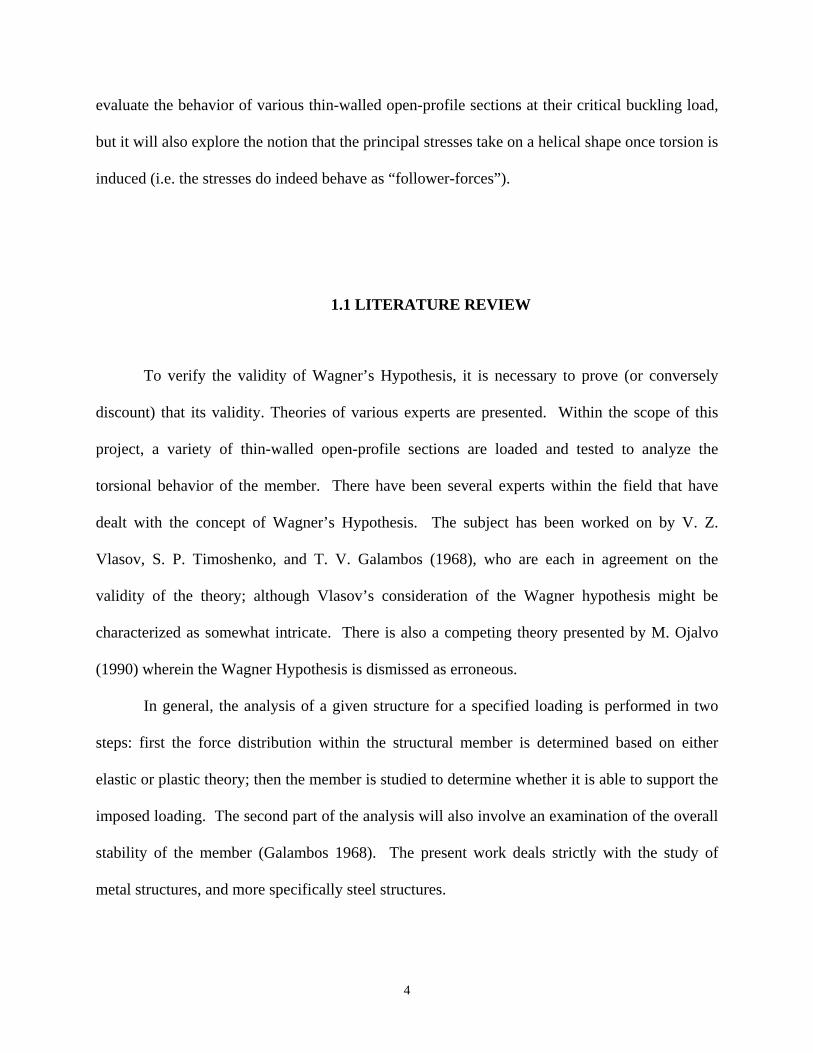
member is not subject to a torsional load, but will exhibit a torsional failure mode. Galambos
developed two differential equations for lateral-torsional buckling for any elastic beam subjected
to in-plane concentrated end moments:
0''2" =++ φφ xxiv
y MMuEI
Eqn. 1-1
0"''")( =+−+− uMMMGKEI xxxxxTiv φβφβφω
Eqn. 1-2
where,
9

0
22
2)(
yI
dAyxy
x
Ax −
+= ∫β
Eqn. 1-3
βx is a property of the cross-section. To apply these equations to a doubly symmetric, simply
supported cross-section, a few manipulations must be made. For a section with double symmetry
it can be shown that,
∫ ∫+
−
+
−=+= t
t
t
t
y
y
x
xx
x dxdyyxyI
0)(1 22β
Eqn. 1-4
and
0MM x =
Eqn. 1-5
0' =xM
Eqn. 1-6
The differential equations now become,
0"0 =+ φMuEI ivy
Eqn. 1-7
10

0"" 0 =+− uMGKEI Tiv φφω
Eqn. 1-8
Once these equations have been integrated, solved and manipulated, the critical moment for a
simply supported, doubly symmetric section is found to be equal to the following:
)1()( 2
22
0 LGKEIn
GKEILnM
TTycr
ωππ+=
Eqn. 1-9
The lowest energy state corresponds to n = 1. The use of this equation will allow for a
comparison with a moment arrived at using a finite element analysis for a simply supported I-
beam. Both the differential equations as well as the equation for critical moment developed in
the theory provided by Galambos employ the Wagner Hypothesis for thin-walled open-profile
sections, and more specifically beams.
The next section of the project deals with columns and their behavior relative to
Wagner’s Hypothesis. Within this study there were two columns modeled in a finite element
analysis and there are theoretical equations presented by both Galambos and Ojalvo. A column
is defined as a member subject to an axial compressive load applied through the centroid, or at
some very small eccentricity; for practical purposes columns typically stand on end. When
evaluating any column member, one of the main concerns is stability. A member loaded by an
axial force may tend to buckle. Within the scope of this study, only long, slender columns will be
considered, and typically this type of column will buckle while the material is still elastic. The
11

practical maximum load that can be carried by an elastic column is the load where the column
buckles (Galambos 1968).
Each of the sections chosen for the finite element analysis is found to be subject to a
buckling failure mode, and in each case the stability of the structure is to be scrutinized.
Instability is a condition wherein a compression member loses the ability to resist increasing
loads and exhibits instead a decrease in load-carrying capacity as deflections increase; therefore
instability occurs at the maximum point on a load-deflection curve (Galambos 1998). To ensure
that each of the finite element models analyzed are achieving accurate results, the stability of
each will be considered. It is known that the critical load of a member subject to compression
does not necessarily equal the load at which a real imperfect member will collapse. To evaluate
the point at which a real member will fail, it is necessary to consider the members’
imperfections. In determining the load carrying capacity of a structural member it is possible
that when subjected to increasing load, a member will initially deform in one mode, then reach a
critical loading, and then continue to deform in a different pattern. This is referred to as the
bifurcation of equilibrium. There are two types of bifurcation buckling for initially perfect
systems depicted in the following diagram:
Figure 3: Postbuckling of Perfect Column. (a) Stable (b) Unstable Curve. (Galambos 1998)
12
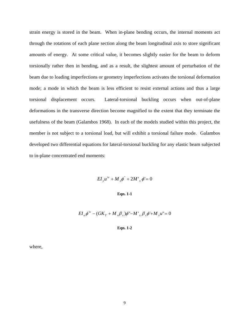
In each of the plots, the member initially deforms in one mode, the prebuckling deformation, and
then at the critical load, due to a branch in the load-deflection curve, the deformation suddenly
changes into a different pattern, the buckling mode. An example of this phenomenon is when an
axially loaded column initially shortens and then bends once it reaches the critical load. The
plots above represent the fact that a structure’s stiffness may increase or decrease at the onset of
buckling. The structure is said to have a stable postbuckling curve if it can support an increasing
load following the onset of buckling. On the other hand if the load decreases, the structure has
an unstable postbuckling curve (Galambos 1998).
The postbuckling curve of an initially perfect system does not by itself give sufficient
information to allow one to determine when failure takes place (Galambos 1998). There are
initial imperfections that exist in all members, and these characteristics of the real structure must
be considered. The load deflection curves for both stable and unstable systems with initial
imperfections are as follows:
Figure 4: Postbuckling Curves for Initially Imperfect Systems. (Galambos 1998)
13

It is obvious from the plots that for a system with a stable postbuckling curve, very small
imperfections have little effect on the behavior of the system. This type of structure is able to
resist increasing loads after the critical load is reached, and a failure will occur only once the
member has yielded. In contrast, for the system that has an unstable postbuckling curve the
initial imperfections have a greater effect on the system, and the member will typically fail at a
load less than the critical buckling load. It is evident that the behavior of real imperfect systems
can be predicted from the shape of the postbuckling curve for perfect systems (Galambos 1998).
Due to this fact, it is reasonable to evaluate the behavior of the columns analyzed using the finite
element method by considering the load deflection plots produced from the output. If the output
generates a plot similar to either stability curve, the user can be confident that the analysis is
giving accurate results. All models included in the present research are analyzed assuming
elastic behavior. When the member is elastic, it will return to its original undeflected position
after loading is removed.
In order to develop the critical moment equations for the final set of finite element
analysis runs, the behavior of elastic beam-columns must also be discussed. A beam-column is
defined as a member that can support both axial compressive loads as well as moment at either
end of the section. There are many practical applications for this type of member. A member is
also considered a beam-column when it is subject to an axial compressive load with some
amount of eccentricity, which produces a moment. The relationship between load and
deformations for beam-columns differs from the behavior seen individually in either beams or
columns. The axial load that is applied to a beam-column may be smaller than the maximum
load that an equivalent column could carry, and therefore there is some reserve of capacity for
moment that can be resisted (Galambos 1968). At the same time the moment that can be carried
14

is less than the full plastic moment that could be resisted by the beam if the axial load were equal
to zero. The system of coupled differential equations governing the elastic behavior of beam-
columns of arbitrary cross-section is (Galambos 1968):
)(])([" 0 xxxyyy BTBBTBx MMLzMPxMM
LzMPvvB +−=++−−+ φ
Eqn. 1-10
)(])([" 0 yyyxxx BTBBTBy MMLzMPyMM
LzMPuuB ++−=−+−−+ φ
Eqn. 1-11
0)(
)(])(['])(['')(''' 00
~
=+−
+−++−−+++−++−
xx
yyyyyxxx
BT
BTBTBTBBTw
MMLu
MMLvPxMM
LzMvPyMM
LzMuKCC φφ
Eqn. 1-12
where the bending stiffness about each principal axis is:
xx EIB =
Eqn. 1-13
and
yy EIB =
Eqn. 1-14
the St.Venant torsional stiffness is
TT GKC =
Eqn. 1-15
15

the warping stiffness is equal to
ωEICW =
Eqn. 1-16
and
∫=A
dAaK 2~ σ
Eqn. 1-17
These equations can be rewritten with the conditions that MBy = MTy = 0, MBx = -M0, and MTx =
kM0 as:
)]1(1[" 00 kLzMPxPvvBx −+−=−+ φ
Eqn. 1-18
0)]1(1[" 00 =+−−++ φφ PykLzMPuuBy
Eqn. 1-19
0)1('')]1(1['')(''' 0000
~=−+−+−−++− uk
LM
vPxuPykLzuMKCC Tw φφ
Eqn. 1-20
It should be noted that these three equations are not independent of one another and that the first
equation is not homogeneous. Lateral-torsional buckling is governed by the second and third
differential equations presented above. After some manipulation and substitution into these
equations, the buckling condition for a beam-column becomes:
16

200000
)())(( PyMMrPPrPP xzy +=+−− β
Eqn. 1-21
where Py and Pz are equal to:
2
2
LEI
P yy
π=
Eqn. 1-22
and
2
0
2
2
r
GKLEI
PT
z
+=
ωπ
Eqn. 1-23
This equilibrium equation can be used to find the critical combination of P and M0 for any beam-
column section (Galambos 1968). Within the scope of this study, this development is used to
compute the critical load for a column subjected to an axial load with a degree of eccentricity.
For beams, columns, and beam-columns, Galambos has developed theoretical equations set forth
by Vlasov and Timoshenko applying principles from the Wagner Hypothesis.
The competing theory presented by Ojalvo to discount the use of the Wagner
Hypothesis includes the development of a new second-order theory for structures subjected to
torsional failure. When developing the second-order theory, Ojalvo states that the line with
which a deformed bar is modeled is the line of centroids. He states that the centroid line is
17

important because the transverse displacement of the centroid of a profile is the average
transverse displacement of a profile and its longitudinal displacement corresponds to the average
longitudinal displacement of the points of a profile (Ojalvo 1990). This differs from the theories
developed by Galambos, which models deformations about the shear center of the section.
Galambos affirms that when the line of shear centers is utilized the Wagner effect must be
employed. The Wagner effect is redefined as the induced torsional moment in a normal plane
arising from longitudinal stresses and twist deformations, and Ojalvo states that he does not
support the use of this pheonmenon (Ojalvo 1990). The second-order theory that he develops is
in complete agreement with classical buckling theory, in that the critical load associated with a
member corresponds to the point where the member initially buckles. He derives equations
associated with the critical moment of a simply supported beam subject to a constant moment,
and the resulting equations presented are identical to the theory that Galambos puts forward.
Ojalvo begins his development of the equations that describe the nature of the buckling
load for the second-order theory with the following differential equations:
0'""'2'''']"2["]'2['''"'''' 0000 =−+++−−+−++−+ xcccycycxcy qvTvTvTqxTVxTPyMxTPuuEI θθθθ
Eqn. 1-24
0"]["][']["]*['''' 00002
000~ =−−+++++−+−+ zyxxyyx mvPxMuPyMxVyVGJrPxMyMEI θθθω
Eqn. 1-25
After some manipulation and substitution, Ojalvo develops an equation from which buckling
loads can be calculated:
18

0)()1()(~~
0
2 =++−−= PPPPPyePPF yy
Eqn. 1-26
where,
0
2~ )( ~
ey
GJEIkP
+= ω
Eqn. 1-27
These differential equations are used as the basis of other numerical solutions specific to the
columns that were used to model the finite element analysis portion of the current study.
Ojalvo plainly states that the notion of longitudinal stresses inducing torsional moment on
normal sections of a deformed bar is not valid (Ojalvo 1990). He therefore denies the possibility
of torsional buckling as an admissible global instability (he instead explains experimental
observations of such response as a by-product of local instabilities). He states that in general, the
equilibrium method derivations in which the Wagner effect terms appear are deficient for not
identifying the free body with which torsional equilibrium is expressed and for violating statical
principles (Ojalvo 1987) (e.g. Navier’s plane-section hypothesis). Ojalvo does not limit his
criticism to only strong form statements of the problem at hand, and he contends that derivations
based on variational methods (Bleich 1952) are just as incorrect, in that the theorem of stationary
potential energy is misused. In other words, the components of a finite strain tensor are used in
the strain energy expression when infinitesimal strain expressions are required (Ojalvo 1982,
1987). He also believes that adopting the line of shear centers without using the Wagner effect
19

leads to at least one major problem, which is that a mono-symmetric I-beam under uniform
moment buckles at the same value of moment regardless of whether the smaller or larger flange
is in compression (Ojalvo 1987). Another mono-symmetric column model will be studied within
the current study to examine this claim.
In the case of the cruciform-shaped column, Ojalvo defines several equations for the
torsional buckling load of the section. The buckling load presented by Ojalvo using the Wagner
effect is:
0"]['''' =−+ θθω GJAI
PEI o
Eqn. 1-28
where Io is the shear center polar moment of inertia of the profile area (Bleich 1952). When θ =
θ” = 0 at either end of the section the critical buckling load is equal to the following:
32
23
2
2
2716
916)( td
LE
dtG
LEIGJ
IAPo
ππωθ +=+=
Eqn. 1-29
The analogous solution that does not employ the Wagner effect is equal to:
32
23
2
22
2 43
49])}2{([4 Etd
LdtG
LdEIEIGJ
aP y
ππωθ +=++=
Eqn. 1-30
20
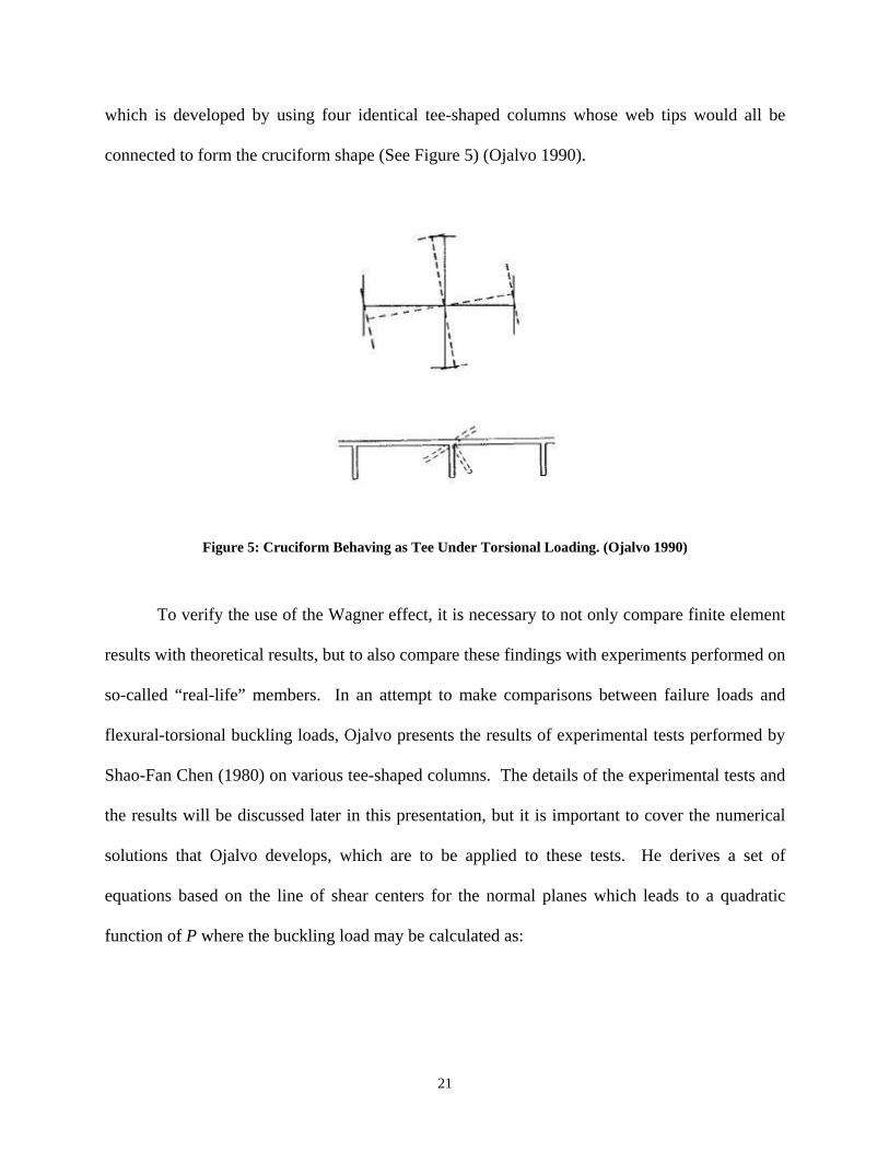
which is developed by using four identical tee-shaped columns whose web tips would all be
connected to form the cruciform shape (See Figure 5) (Ojalvo 1990).
Figure 5: Cruciform Behaving as Tee Under Torsional Loading. (Ojalvo 1990)
To verify the use of the Wagner effect, it is necessary to not only compare finite element
results with theoretical results, but to also compare these findings with experiments performed on
so-called “real-life” members. In an attempt to make comparisons between failure loads and
flexural-torsional buckling loads, Ojalvo presents the results of experimental tests performed by
Shao-Fan Chen (1980) on various tee-shaped columns. The details of the experimental tests and
the results will be discussed later in this presentation, but it is important to cover the numerical
solutions that Ojalvo develops, which are to be applied to these tests. He derives a set of
equations based on the line of shear centers for the normal planes which leads to a quadratic
function of P where the buckling load may be calculated as:
21

0)2()}{2( 220
2
2
=++⎥⎥⎦
⎤
⎢⎢⎣
⎡−−−+
⎥⎥⎦
⎤
⎢⎢⎣
⎡
yyxp
yyyxp
y PGJer
PPeyer
PP ββ
Eqn. 1-31
in which,
∫ −+=A
xx yydAyx
I 022 2)(12β
Eqn. 1-32
He also develops a quadratic function from which the buckling load can be calculated based on
the theory of the line of centroids defining the normal plane. It is developed from eqn. 1-25
presented previously in this discussion.
0}{}){( 000
2
=+⎟⎟⎠
⎞⎜⎜⎝
⎛+−
⎥⎥⎦
⎤
⎢⎢⎣
⎡−−
⎥⎥⎦
⎤
⎢⎢⎣
⎡
yyy
yyy
y PGJ
PGJeyy
PPeye
PP
Eqn. 1-33
In an effort to verify the development of this new theory, the steps that Ojalvo lists for derivation
of this equation were worked through, and it was not possible to achieve this final buckling
equation. Therefore, when calculating the critical load for the tee-shaped column, eqn. 1-25
from this discussion was utilized (i.e. an error was found in Ojalvo’s book indicating that eqn. 1-
32 does not emanate from eqn. 1-25).
In an attempt to prove conclusively that the Wagner effect does exist, it is necessary to
examine, firsthand, the paper of Shao-Fan Chen (1980) concerning the experimental tests
performed on various tee-shaped columns at the Xian Institute of Metallurgy and Construction
22

Engineering, which is located in Xian, Shaanxi, China. A tee is a mono-symmetric section, and
when acted on by an eccentric load, either a positive or negative eccentricity will exist. Chen
states that based on an analytic study, most cases where this type of member fails under a lateral-
torsional buckling mode, the resistance of the section will be smaller when there is the case of
negative eccentricity (Chen 1980). Chen tested 24 columns with 18 sections experiencing a
negative eccentrically placed axial compressive load. This current research makes use of what
was designated a “PD” section (by Chen), therefore only that section will be covered in this
discussion. This member is built-up using two plates welded together to form tee shapes with
width to thickness ratios of 15. Each classification was given three column lengths. The
members were also assigned an eccentricity ratio defined as:
weA=ε
Eqn. 1-34
where e is defined as the eccentricity, A is equal to the cross-sectional area, and w is the section
modulus. This ratio differs with the various specimens, and each “PD” section was given a
negative eccentricity ratio. The specimens are reported to be made of low carbon steel number 3,
and each “PD” member had a mark of AD3. The members were hinged at each end and were
supported by knife edges, where the center of the hinge was located at the load application point.
The knife-edge at the top of the column was fixed to the testing frame with bolts, while the
knife-edge at the bottom rested on the hydraulic jack. The loading during the test was stepped
according to an estimated ultimate load and was tested until failure.
23

Overall, the 24 specimens saw three different failure modes including local buckling, in-
plane stability, and lateral-torsional buckling. The PD3-1 was chosen for the finite element
model in the current study due to a lateral-torsional buckling failure mode reported in the results
from Chen’s tests. Chen concludes from the results of the experiments that the width to
thickness ratio for a tee-section should be limited by a slenderness ratio much like an I-section
(Chen 1980). He also discusses equations related to the critical buckling load of the tee-section,
but his formulation was not studied within the scope of this project; only his raw experimental
results were of interest.
Within the literature presented by each of the authors including Galambos (1968), Ojalvo
(1990), and Chen (1980), there are separate formulations for the critical buckling loads
associated with different types of structural members. Galambos further develops a second-order
theory based on the works of Vlasov and Timoshenko, which use the line of shear centers by
which to model their numerical solutions. These solutions include the use of the Wagner
Hypothesis. Ojalvo presents a competing theory where the Wagner effect is disregarded and the
line of centroids is used to develop a substitution for the classical second-order theory by which
to calculate the critical buckling loads for various members. Experimental tests performed by
Chen are used to verify both theories.
1.2 OVERVIEW OF THESIS ORGANIZATION
Chapter 2 discusses the finite element method as it applies to the current study. Section
2.1 covers the procedure for modeling a structure using the finite element method, analyzing the
24

structure, and interpreting the results. It outlines the importance of the element mesh as well as
mathematical models used to solve the models. Chapter 3 covers the finite element model used
to verify that ABAQUS 6.4 would be an adequate tool for analyzing the models related to the
problem at hand. Within the contents of Chapter 4, various models are analyzed in order to
compare the finite element results for beam and column behavior to theoretical results provided
by both Galambos and Ojalvo. Chapter 5 encompasses the results of the current study as well as
conclusions that can be drawn from those results.
25

2.0 FINITE ELEMENT METHOD
The objective of the current study is to determine the validity of the Wagner Hypothesis as it
relates to classical theories regarding lateral-torsional buckling of thin-walled open-profile
members. The Finite Element Method (FEM) is employed in this research to create analytical
models of thin-walled open-profile sections. In general, the finite element method is a numerical
method for solving engineering problems which have complicated geometries, loadings, and
material properties. It allows the user to solve complex problems without the requirement of the
direct solution of ordinary or partial differential equations. The FEM analysis will result in a
system of simultaneous algebraic equations for the solution, as opposed to a very complicated
and almost impossible solution of differential equations. The method assembles a finite number
of structural elements interconnected by a finite number of nodes. The analysis will provide an
approximate solution to the actual structure since the original continuum is divided into an
equivalent system of finite elements using one-, two- and three- dimensional structural elements.
The material properties for the system will be retained by the elements chosen as part of the
analysis. The commercial multipurpose finite element software package, ABAQUS 6.4, is
employed in this research to execute nonlinear finite element analysis studies. Only geometric
nonlinearity is considered herein.
26

2.1 FINITE ELEMENT ANALYSIS PROCEDURE
The process of modeling a body and analyzing that body under a particular loading
begins with the discretization of the body into an equivalent system of smaller units (finite
elements) interconnected at points common to two or more elements (nodes). An appropriate
element type is chosen to closely simulate the behavior of the original continuum. In general,
smaller elements are used to create a denser mesh which will produce better results from the
model. In theory, when the mesh size of correctly formulated elements is reduced, the solution
of the analysis will converge to the exact solution for the actual structure. The compatibility of
elements with adjacent elements is very important for the proper convergence of the analysis. If
the compatibility of the elements is not satisfied, gaps or overlaps within the model will occur,
and may result in a less predictable convergence characteristic.
The evaluation of the element properties for the model involves developing the stiffness
matrix for the given system which forms the relationship between the forces and displacements
in the model. The individual element equations will be superimposed using the direct stiffness
method to produce the global stiffness matrix, [K]. The following equation relates the forces, F,
to the displacements, d, for the system using the global stiffness matrix, [K]:
{ } [ ]{ }dKF =
Eqn. 2-1
Boundary conditions must be imposed in order for numerical singularity to be avoided, so that
the structure remains stationary during the analysis instead of moving as a rigid body.
27

Following the evaluation of the element properties, the actual analysis of the structural
model must be completed. In order for the analysis to run correctly, the equilibrium,
compatibility, and force-displacement relationships must be satisfied. The equations that result
from the force-displacement relationships may be solved using the force method approach or the
displacement method approach, both of which are appropriate for structural systems that are
elastic. The mathematical system may be solved using any number of solution algorithms
including elimination methods such as Gaussian elimination or iterative methods including the
Gauss-Seidel method. For a nonlinear analysis, these methods are not sufficient to directly arrive
at an equivalent approximate solution, and therefore the equilibrium path must be traced using
iterative and incremental methods.
2.2 NONLINEAR FINITE ELEMENT ANALYSIS
To evaluate a problem of linearly elastic nature a linear analysis of the structure is
performed, because it is assumed that the displacements of the members are infinitesimally
small. Nonlinearity in structures can be classified as either material or geometric nonlinearity.
Material nonlinearity results from changes in the material properties, such as plasticity, and
geometric nonlinearity can result from changes in the configuration of the model, such as large
deflections. A change in the geometry in the model may cause both the load distribution and
magnitude to be altered.
During a nonlinear analysis the solution cannot be calculated by solving a system of
linear algebraic equations directly. The solution is found by specifying the loading as a function
28

of time and incrementing the time intervals to obtain the nonlinear response (the term “time” is
used in a generic sense since all analysis considered herein are static and thus time is a “dummy”
variable used to connote incrementation of load). ABAQUS breaks the given analysis into a
predetermined set of time increments and calculates the approximate equilibrium configurations
at the end of each time period. ABAQUS assumes the response to be linear within each interval.
After each increment, the structure is reconfigured and a new ideal linearized structural response,
or tangent stiffness matrix, is calculated. For each increment, the linearized structural problem is
solved for displacements, and these displacements are added to those determined at the end of
the previous increment. ABAQUS uses the load proportionality factor as the load increment, and
the load proportionality factors will vary in size as a function of the effort required to achieve
convergence in the prior increment. After each converged increment is computed, the program
will compute a new tangent stiffness matrix using the internal loading and the deformation of the
structure at the beginning of the load increment. The tangent stiffness matrix, [kT], may be
denoted as:
[ ] [ ] [ ]poT kkk +=
Eqn. 2-2
where [kO] is the common linear stiffness matrix for the uncoupled bending and force behavior,
and the matrix [kP] is the initial stress matrix that is based on the force at the beginning of each
load increment.
29
2.2.1 Nonlinear Equilibrium Solution Methods
For the current research, incremental solution procedures are necessary to trace the
nonlinear equilibrium path of the model. ABAQUS utilizes either the Newton-Raphson
Algorithm or the modified Riks-Wempner Method (arc length method) (ABAQUS 2003); both
methods are powerful tools for determining the nonlinear response of a system. ABAQUS uses
the Newton-Raphson method as its default solution algorithm. This method is useful for cases
where there is mild nonlinear response. The Newton-Raphson method is advantageous because
of its quadratic convergence rate when the approximation at a given iteration is within the radius
of convergence (ABAQUS 2003). One drawback of this technique is its inability to traverse
limit points in the equilibrium path being traced as part of the nonlinear solution process. The
Riks-Wempner method does not suffer from this limitation and as such represents the solution
strategy of choice when tackling problems with large degrees of nonlinearity.
2.3 ELEMENT TYPE
Shell elements found in the ABAQUS element library are chosen for this study due to
their ability to economically model structures where one dimension, the thickness is much
smaller than the other dimensions of the structure. A three-dimensional shell element is able to
model either “thick” or “thin” shell problems. The nonlinear shell element chosen for various
modeling applications throughout this project is the S4R shell element (ABAQUS 2003). The
S4R element is defined by ABAQUS (2003) as a 4-node doubly curved general-purpose shell,
with reduced integration, hourglass control, and finite membrane strains.
30

There are five aspects of an element that characterize its behavior. They include:
1. Family
2. Degrees of Freedom
3. Number of Nodes
4. Formulation
5. Integration
The S4R belongs to the shell family, and it possesses 4 nodes. There are two types of shell
elements, thick and thin shells. Thick conventional shell elements are utilized in cases where
transverse shear flexibility is important and second-order interpolation is desired (ABAQUS
2003). Thin conventional shell elements are used for modeling cases where transverse shear
flexibility is negligible and the shell normal remains orthogonal to the shell reference surface.
The general purpose conventional shell elements used in this research allow transverse shear
deformation, and they use thick shell theory as the shell thickness increases and become discrete
Kirchoff thin shell elements as the thickness decreases (ABAQUS 2003). This is important for
this project because the shell thicknesses are changed for varying sized columns and beams. For
each of the four nodes on the element there are six active degrees of freedom, which include
displacements and rotations in each principal direction. The S4R element degrees of freedom are
defined as:
1, 2, 3, 4, 5, 6 (ux, uy, uz, φx, φy,φz,)
The S4R element uses reduced integration to form the element stiffness matrix, while the
mass matrix and distributed loadings are integrated exactly. Reduced integration usually
31

provides more accurate results (e.g. relieves shear locking, etc.), provided that the elements are
not distorted or loaded in in-plane bending, and it significantly reduces the running time for the
model resulting in a more economical choice for the user (ABAQUS 2003). The S4R is said to
be computationally inexpensive since the integration is performed at one Gauss point per
element.
Figure 6: S4R Element
2.4 FINITE ELEMENT MESH
The analytical models created for this study are built from a dense finite element mesh of
the ABAQUS S4R element described in the previous section. The mesh density is directly
related to the computational time and the modeling accuracy. These two factors must be
balanced in such a way that the model produces relatively accurate results while being analyzed
32

in an appropriate amount of time. The finer the mesh density is, the more accurate the results
will become, but the computational time will also increase.
The elements used in each of the models including the verification study have an aspect
ratio of one-to-one. In other words, all elements in each of the models have a square shape. The
mesh density employed herein was proven to provide accurate results at both the local and global
level, in the verification work provided by Earls and Shah (2001). The equally sized elements in
the flanges and webs of each model allow the components to be compatible. This means that the
mesh along the web segment can be integrated with the longitudinal mesh of the flange sets.
This allows the user to accurately tie the meshes of separate elements together to make a single
piece that performs as one.
2.5 IMPERFECTION SEED
In modeling studies where buckling is investigated, it is important that the evolution of
the modeling solution be carefully monitored so that any indication of bifurcation in the
equilibrium path is carefully assessed so as to guarantee that the equilibrium branch being
followed corresponds to the lowest energy state of the system (Earls and Shah 2001). To ensure
that the lowest energy path is followed, the current study uses an imperfection seed in the finite
element analysis with some initial displacement or rotation. This initial displacement is obtained
from a linearized-eigenvalue buckling analysis where an approximation of the buckling mode is
found. This analysis will indicate which mode should be used as well as the initial displacement.
This is then superimposed onto the finite element mesh in order to perform a postbuckling
33

analysis. The imperfection seed is scaled so that the maximum initial displacement is small
enough so as to not affect gross cross-sectional properties of the model (Earls and Shah 2001).
In order to find an accurate account of the critical loads achieved by the model, various scale
factors are used. Although the technique of seeding a finite element mesh with an initial
imperfection to ensure that the correct equilibrium path is followed is recognized to have
shortcomings, the technique is employed in this project due to the fact that the results obtained
from this method have agreed with experimental tests (Earls and Shah 2001). The imperfection
seed is superimposed on to the mesh by using the *IMPERFECTION command in the ABAQUS
finite element software.
2.6 MATERIAL PROPERTY DEFINITIONS
Steel is the material used for each of the models presented in this study, due to its
widespread practical use. The input file for the finite element analysis requires that the material
properties for each section of the model are defined appropriately. All analysis performed within
the scope of this project is purely elastic. A material name is coded into the input file with a
modulus of elasticity, E, and Poisson’s Ratio, ν, for the analysis. In each of the models used in
the current study, the modulus of the elasticity used is 29,000 ksi, and Poisson’s Ratio is 0.3; this
is typical for all grades of structural steel.
34

3.0 VERIFICATION STUDY
In order to create models using the finite element method, and to ensure that the analysis
produces reliable results, the modeling techniques must be verified using a reliable data set. For
the current project, a numerical model was selected from Galambos’ text (1968) to recreate the
variation of curvature, Φ, along the length of the beam. The model prescribed a W12x50 steel
shape, simply supported, with an eccentric load at the mid-span of the structure.
ABAQUS was used to model the beam using the geometry and material properties
described in the text. The beam was constructed by defining nodes, and then creating node sets
and elements between those nodes; the elements used for this model are shells designated S4R.
Each element corresponded to regions with separate material properties and shell thicknesses.
The accuracy of the finite element analysis is dependant on the density of the mesh for the
model. A dense mesh is used for all of the models throughout the project to obtain more
accurate results, and an aspect ratio of one-to-one is maintained for all elements in these models.
The element size is one square inch. For the verification study, the model generated includes
approximately 7,000 nodes and 6,800 elements.
3.1 VERIFICATION STUDY RESULTS
The objective of the verification study chosen is to replicate the rate of curvature versus
length curve presented by Galambos. Young’s Modulus is set to 29,500 ksi and Poisson’s Ratio
is 0.3 in the finite element model. The example uses a W12x50 wide flange section where the
35
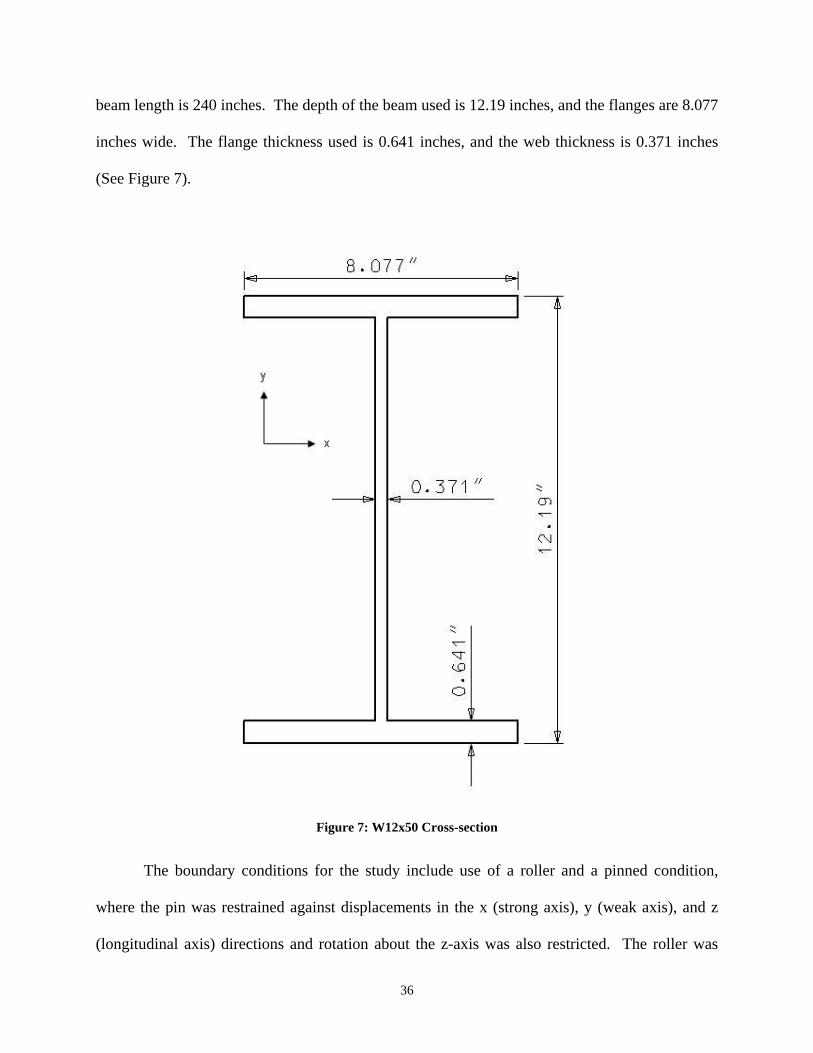
beam length is 240 inches. The depth of the beam used is 12.19 inches, and the flanges are 8.077
inches wide. The flange thickness used is 0.641 inches, and the web thickness is 0.371 inches
(See Figure 7).
Figure 7: W12x50 Cross-section
The boundary conditions for the study include use of a roller and a pinned condition,
where the pin was restrained against displacements in the x (strong axis), y (weak axis), and z
(longitudinal axis) directions and rotation about the z-axis was also restricted. The roller was
36

restrained against displacements in the x and y directions, and rotation about the z-axis was again
prohibited. The rotations were restrained so that the beam would not completely overturn while
being loaded. So that the beam would be permitted to twist at the mid-span, rigid beam elements
were employed at the support locations. These “rigid beam” elements were given an elastic
modulus, E, ten times greater than the elastic modulus of the steel, as well as cross-section
dimensions of five inches in length by five inches in width.
The load, Q, was applied with an eccentricity, e, to produce a twisting moment equivalent
to,
eQM z ∗=
Eqn. 3-3-1
about the shear center of the cross-section. In order to model the eccentricity of the load, a small
lever arm is attached to the beam at the mid-span of the beam at the center of the web. This arm
is comprised of rigid beam elements so that the arm itself would not deform when loaded. It is
not necessary that the arm see any portion of the load, and therefore the rigid beam elements
allow the load to be transferred totally to the beam. The actual load for the example was not
stated in the text; therefore, the end of the lever arm is loaded with a one kip load acting in the
downward y direction.
When viewing the deformed shape through the ABAQUS 6.4 CAE viewer, it is obvious
the beam is experiencing a lateral-torsional buckling mode of failure.
37

Figure 8: Deformed Shape of a Simply Supported Beam under Eccentric Loading
The plot developed by Galambos shows a curve of the location on the beam, z, divided by the
total length of the beam versus a non-dimensionalized unit of the variation of the curvature.
38

Figure 9: Variation of Angle of Twist and Derivatives Along Beam Length. (Galambos 1968)
Once the finite element model of the beam is built, it is important to duplicate this curve in order
to verify that ABAQUS is providing accurate results. The rotation of the beam about the
longitudinal, or z-axis, is exported from ABAQUS into Microsoft Excel. This rotation is
reported at the intersection of top flange and web. The rotation, φ, is then non-dimensionalized
in the same fashion as listed in the text. The rotation is multiplied by a unit-less factor of:
39

LMGK
z
T2
Eqn. 3-3-2
which for this case yields a value of 174.4. The plot derived from the finite element analysis
results is the following:
Rotation About the Longitudinal Axis
0.00E+00
5.00E-02
1.00E-01
1.50E-01
2.00E-01
2.50E-01
3.00E-01
3.50E-01
0 0.1 0.2 0.3 0.4 0.5 0.6 0.7
z/L
2GKt
φ/M
zL
Figure 10: Rotation about Longitudinal Axis of W-Section Compared to Galambos’ Plot
The maximum curvature achieved from the plot given in the text is approximately 0.30 radians.
This value has been scaled off of the plot which was reproduced from the text. The finite
element analysis results provide a maximum curvature of 0.319 radians. Therefore, the results of
the verification study are satisfactorily showing that the ABAQUS finite element analysis
software is a reasonable tool for producing models within an appropriate degree of accuracy for
this study. The research will make use of the software to evaluate torsional deformations for
40

beams and columns in relation to their failure modes. Also, the models will be evaluated
regarding the stresses relative to the theories presented.
41

4.0 FINITE ELEMENT MODELS
To support the existence of the Wagner Hypothesis, it is necessary to find compatibility between
the results of finite element analyses, theoretical solutions, and experimental test results relative
to the theory. A new second-order theory pertaining to thin-walled open-profile sections has
been developed by Ojalvo in opposition to the classical theory that states when a bar is subject to
an axial load and the section twists, the longitudinal stresses become inclined to the normal plane
and produce a torsional moment in that plane. So that the classical theory may be verified,
several different finite element models are created using the ABAQUS finite element analysis
software so as to produce modeling results to compare with both second-order theories as well as
experimental results. In making these comparisons, the validity of the competing theory
presented by Ojalvo can be tested. The first model is similar to the verification study presented
in the previous chapter. It is a doubly symmetric W-section that is loaded by a uniform moment
across the length. A linearized-eigenvalue buckling analysis is performed on the model to find
the critical buckling load; this value is then compared to the numerical solution applied to the W-
section, which was provided by Galambos (1968).
Subsequent models are created to compare the new theories derived by Ojalvo to the
classical theories further developed by Galambos. Along these lines, a second model is
developed; a cruciform-shaped column that is axially loaded through the section’s centroid. A
linearized-eigenvalue buckling analysis is performed to capture the buckling mode of the column
so that it can be utilized as an initial imperfection. This imperfection is then superimposed onto
the column so that a postbuckling analysis can be performed to determine the critical buckling
load of the structure. This value is compared to numerical solutions provided by both Galambos
42

and Ojalvo to determine whether the Wagner effect should be included in the second-order
theories. The third and final finite element analysis is performed on a tee-shaped column that is
loaded axially through a point of eccentricity. The consideration of these modeling results is
essential since the cross-section is a mono-symmetric shape and thus offers the opportunity for
important insights to be gained. The tee finite element analysis is performed in the same way
that the cruciform is analyzed with an initial imperfection and a postbuckling analysis to
determine the value of the critical buckling load. Not only are these results used for comparison
with numerical solutions derived by Galambos and Ojalvo, but since the model is an analog to an
actual experimental test specimen (Chen 1980); the results can be verified against the critical
loads provided by the test results. The comparisons made in this chapter will give a solid
indication as to whether the Wagner effect should be included in the second-order theories
developed relative to the torsional behavior of open-profile thin-walled sections.
4.1 DOUBLY SYMMETRIC W-SECTION LOADED BY UNIFORM MOMENT
The finite element model that is used to verify that ABAQUS could achieve accurate
results for this research is now modified to compare with theoretical equations provided by
Galambos (1968). The model consists of a simply supported W12x50 section, which is specified
as 240 inches in length. The cross-sectional shape has a flange width of 8.077 inches with a
0.641 inch thickness. The web depth is 11.5 inches with 0.371 inch thickness. The modulus of
elasticity is given as 30,000 ksi, and the shear modulus is 11,500 ksi. The moment of inertia
about the y-axis is 56.4 in4, while about the x-axis the moment of inertia for the section is 394.5
43

in4. The warping moment of inertia, Iw, is equal to 1,881 in6 and the St.Venant torsion constant,
KT, is 1.82 in4. The finite element model is built by defining node locations according to the
shape of the beam and then filling in those nodes with elements to create a mesh with an aspect
ratio of one-to-one. The element chosen for this model is an S4R shell element, and the element
size is one square inch. This particular element gives accurate results while keeping the
computational time of the models to a reasonable level. Along the outside middle lines of the
cross-sections occurring at the member ends, rigid beam elements are placed between all nodes
along the web to facilitate the imposition of idealized boundary conditions without producing
unwanted warping restraint. With the use of the rigid beam elements, a single boundary
condition can be placed at the mid-height of the section at either end of the beam. At one end the
model is restrained against displacement in the x (stong axis), y (weak axis), and z (longitudinal
axis) directions as well as rotation about the z-axis is prohibited. At the other end of the section,
displacements in the x and y directions are restrained as well as the rotation about the z-axis.
The rotation about the z-axis is restrained so that the model is able to twist at locations within the
span length, while no twist is permitted to occur at the ends. The model is loaded at the
boundary with a constant moment of 6000 kip-inches which grows according to the magnitude of
a load proportionality factor that is determined as part of the nonlinear solution process in
ABAQUS.
Owing to the fact that geometric or material nonlinearities may occur during the analysis
of the section, a command line is included in the ABAQUS input deck to indicate whether these
nonlinearities should be considered. For this analysis, the model uses 30 time increment steps
and the results will include geometric nonlinearities that may arise during the model’s execution;
material nonlinearity is not considered. A static analysis is the contextual basis for the modeling
44
(i.e. the loads are applied slowly), and the Modified Riks method (ABAQUS 2003) solution
technique is employed as part of the postbuckling analysis. The Modified Riks method is
typically used to predict unstable, geometrically nonlinear collapse of a structure (ABAQUS
2003). There is an indication that the beam has reached the critical buckling load once a
negative eigenvalue emerges in the numerical analysis (i.e. a negative eigenvalue is detected in
the global stiffness matrix of the entire model). The occurrence of this first negative eigenvalue
needs to also occur in the time step following the increment where it first appeared to ensure that
the buckling mode is persisting (i.e. not subsequently eliminated by a reduction of the load
proportionality factor). These eigenvalues are easily obtained from the message file produced by
the analysis. The message file will give information regarding the progress of the solution as
ABAQUS executes the file. It lists details including increment numbers, step times, equilibrium
iterations, the load proportionality factor associated with the Riks analysis, etc. The load
proportionality factor can be described as the fraction of the load that the model is seeing at a
particular point in time, with the point in time being a specific increment. For this model, the
first negative eigenvalue occurs at time increment nine, which corresponds to a load
proportionality factor of 0.5025, or about fifty percent of the total load. This results in a critical
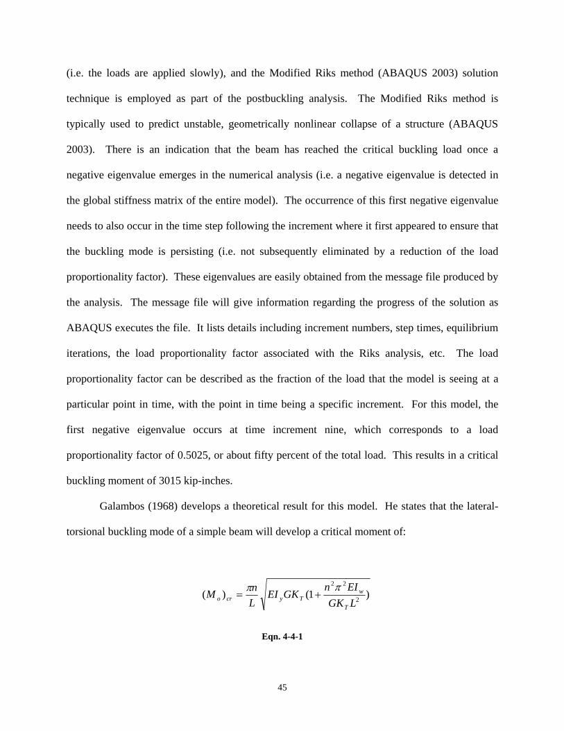
buckling moment of 3015 kip-inches.
Galambos (1968) develops a theoretical result for this model. He states that the lateral-
torsional buckling mode of a simple beam will develop a critical moment of:
)1()( 2
22
LGKEIn
GKEILnM
T
wTycro
ππ+=
Eqn. 4-4-1
45

Setting “n” equal to one, the critical moment is calculated as 2978.52 kip-inches. The difference
in the theoretical value and the result of the finite element analysis equals 1.2%, which proves
that the finite element analysis results for this case are in definite agreement with the use of the
Wagner Hypothesis.
4.2 FLANGED CRUCIFORM COLUMN LOADED BY AXIAL FORCE
A second finite element analysis is executed to further prove the validity of the Wagner
Hypothesis. A flanged cruciform model presented by Ojalvo is utilized as the subject of this
analysis. The column is a shape with length, L, and thickness, t; where t is very small when
compared with its other dimensions. The area of the section is defined as 12td, where d is the
length of a flange piece. The depth and width of the cross-section are defined as 4d. The polar
moment of inertia, J, is defined as 4t3d, and both Ix and Iy are equal to 13.5td3. The warping
torsion constant, Iω, is 4/3 td3. For the initial model, a trial thickness of t = 0.1 inches, a depth of
d = 6 inches, and a length of L = 240 inches is used because actual dimensions were not provided
by Ojalvo. Using these dimensions, the area of the section is 7.2 in2, the polar moment of inertia
is 0.024 in4, both moments of inertia are 291.6 in4, and the warping torsion constant is equal to
28.8 in4. A graphical depiction of the cross-section is shown below:
46

Figure 11: Cruciform Column Cross-sectional Dimensions
Because of the shape of the model, the two sections of the web and the four flanges are
generated separately and then meshed together for the finite element analysis. The outline of the
model is assigned nodes and then this outline is filled with nodes using the node generation
command. The element generation is based on the specified nodes using an aspect ratio of one-
to-one, with the element size being one square inch. The material properties for the cruciform
model are assigned a modulus of elasticity of 29,000 ksi and Poisson’s ratio of 0.3, which are
typical properties of steel. Along the middle lines of the constituent plate surfaces at each end of
the model, there are rigid beam elements placed between the nodes along the web members only
47

so that there is no warping restraint at the ends of the column. While it is that twisting of the
members’ ends is constrained, cross-sectional twisting within the span is unrestrained. These
“rigid beam” elements are given a modulus of elasticity of 290,000 ksi and Poisson’s ratio of 0.3.
Since the outside surfaces are very rigid, the boundary conditions can be placed at the
intersection of the two web sections at a single node location. At one end of the model, the
column is restrained against displacements in the x, y, and z directions, and it is prohibited from
twisting about the y-axis. At the other end of the column, the model is prevented from
displacing in the x and z directions, as well as being restrained against rotation about the
longitudinal y-axis. An axial compressive load of 100 kips was placed at the intersection of the
two web sections at the top of the column; this is subsequently scaled according to the load
proportionality factor. The model geometry required approximately 20,000 nodes and 18,000
elements. For comparison, this model is subject to a number of different analysis runs. The goal
of this phase of the analysis is to compare the finite element results to the second-order theories
provided by Ojalvo, as well as to provide plots of the load versus deflection so that the stability
of the model may be evaluated.
The finite element analysis makes use of an imperfection file to account for initial
imperfections in the model. Two analysis runs are performed: the first to arrive at the probable
collapse mode, and the second to perform the postbuckling analysis. In the first analysis run a
linearized-eigenvalue buckling analysis is executed on the perfect column to find the buckling
mode and to ensure that the mesh discretizes those modes correctly. These results are written to
a “node file” to subsequently be used as input into the postbuckling analysis as an initial
displacement field. The imperfection is superimposed into the code using a single scale factor
applied to the point of maximum displacement to define the maximum perturbation of the model,
48

and the amount of remaining imperfection inputted into the model is determined by relative
scaling of the user input maximum at other locations. This scale factor is adjusted and evaluated
to determine the structure’s sensitivity to the imperfection seed. During the linearized-
eigenvalue buckling analysis run, the model is set up to evaluate the first five buckling modes.
For the first set of models, a series of scale factors was used ranging from L/100 to L/5000. As
the scale factor becomes smaller, the imperfection also becomes smaller and the model parallels
practical conditions. To utilize the imperfection command, the buckling mode retrieved from the
linearized-eigenvalue buckling run must be inputted as well as the scale factor. The ABAQUS
CAE pre- / post-processing software is used to look at each of the five buckling modes from the
linearized-eigenvalue buckling analysis. Mode one corresponds to a twist about the longitudinal
axis, and thus is used with the imperfection command as the seed displacement.
When the postbuckling analysis is complete, the ABAQUS CAE module is used to export
the load proportionality factors as well as the rotation of the model about the y-axis (e.g. 2-axis
in Figure 13). An Excel plot of the load versus deflection is then created for the model; this plot
is used to study the torsional stability of the model. If the plot shows a smooth curve resembling
the stability curves for an imperfect system, then the results are usable. The node located at the
point of intersection of the two webs at the mid-height of the cruciform-shaped model is selected
to provide the output of the load proportionality factors and rotations. The load versus deflection
plot for this set of analysis runs shows various discontinuities in the rotation as the load
approaches a critical value. As can be seen in the Excel plot below (See Figure 12), the curve
does not resemble either of the stability plots that were discussed earlier in this text. Also note
that while the shape of the plot is chaotic, there is no significant amount of deformation about the
longitudinal axis. This discontinuity could be attributable to the fact the Modified Riks analysis
49

method is passing over the critical buckling load through its selection of load increments that are
too large for the present investigation. This occurs when the model has an easy time converging
during the solution process, and as a result permits the incremental load proportionality factors to
grow large. By invoking the direct analysis parameter, the user may specify a constant load
increment size and thus ensure that the critical load is not skipped. In addition, the ABAQUS
CAE viewer is used to analyze the change in deformations as the model was stepped through the
analysis.
Load vs Deflection 0.1" Thickness
0
0.5
1
1.5
2
2.5
3
3.5
4
4.5
5
-1.E-13 -5.E-14 0.E+00 5.E-14 1.E-13 2.E-13 2.E-13 3.E-13 3.E-13
Rotation of Centroidal Node (Radians)
Load
Pro
porti
oalit
y Fa
ctor
Figure 12: Load vs. Rotation for Section having t = 0.1
Through the use of ABAQUS CAE, it becomes obvious that the deformed shape exhibits
the presence of local buckles along the length of the model (See Figure 13). This would cause
50

the local rotation of a node to be in the opposite direction in comparison to the global rotation of
the model. At some locations along the length of the model, the local buckles caused the model
to see a negative value for the rotation about the y-axis.
Figure 13: Mode 1 Deflected Shape of Cruciform Column Exhibiting Local Buckles
Once it is established that the occurrence of local buckles is causing the global critical load to be
undetectable, it is necessary to re-evaluate the parameters of the model, and it is concluded that
the thickness of 0.1 inches is not adequate for the column under consideration, and therefore the
thickness of both the flange plates and web plates is increased to 0.25 inches. This increases the
51

area of the model to 18 in2, the polar moment of inertia to 0.375 in4, both moments of inertia to
729 in4, and the warping torsion constant to 72 in4.
When performing the finite element analysis on the cruciform-shaped column with the
new thickness of 0.25”, another linearized-eigenvalue buckling analysis is run to create the initial
imperfection for the new model. After considering the five buckled shapes provided by the
analysis, it is concluded that the mode 1 buckled shape should be used with a scale factor of
L/1000 (the maximum out-straightness permitted by current steel design specifications) in the
postbuckling analysis. The mode 1 buckled shape is shown below:
Figure 14: Mode 1 Buckled Shape of Cruciform Column with 0.25" Thickness
52

The image provided by the ABAQUS viewer shows the column experiencing a torsional
deformation; with the section twisting once along the length of the column (i.e. torsional mode
1). This imperfection is superimposed into the postbuckling analysis; subsequently leading to
the torsional buckling mode of failure seen in the following ABAQUS screen capture (from the
postbuckling analysis):
Figure 15: Postbuckled Shape of Cruciform Column with Scale Factor of L/1000
53

A plot of the load versus deflection verifies that the model is responding to the axial load as it
should (See Figure 16). It can be seen that as the load increases so does the rotation of the
model, which is consistent with intuition.
WEB UR2 vs. LPF
0.001.002.003.004.005.006.007.008.009.00
10.00
0.00 0.20 0.40 0.60 0.80 1.00
Rotation of Centroidal Node (Radians)
Load
Pro
porti
onal
ity F
acto
r
L/1000 L/500 L/2000
Figure 16: LPF vs. Rotation about Longitudinal Axis for Web Intersection at Mid-height
This plot also demonstrates the relative stability of the model; it can be stated that the model
follows a curve such that after the member reaches a critical load, the member continues to be
loaded and shows the capacity to resist additional load (i.e. stable postbuckling response). The
modeling results indicate that the cruciform-shaped model possesses a critical load of 206.75
kips. This is extracted from the Excel plot at the point where the graph begins to turn and
display a dramatic increase in the twisting deformation. These results are reasonable because the
54

deformed shape of the postbuckling analysis exhibits a purely torsional mode of failure (See
Figure 15).
The form of the classical second-order theory pertaining to the cruciform case appears as:
32
23
2
2
0 2716
916 td
LE
dtG
LEIGJ
IAP ππ
ωθ +=⎟⎟⎠
⎞⎜⎜⎝
⎛+=
Eqn. 4-4-2
Ojalvo, however, rejects the Wagner Hypothesis, as implied in the foregoing equation, and thus
states that buckling of a cruciform, that is purely torsional, is fictitious and thus not covered by
his new theory. He then assumes that the cruciform will behave in the same way that four tee-
columns buckling simultaneously would respond to an axial compressive loading. The critical
buckling load is then given as:
32
23
2
22
2 43
49})2{(4 Etd
LdtG
LdEIEIGJ
aP y
ππωθ +=⎥
⎦
⎤⎢⎣
⎡++=
Eqn. 4-4-3
When evaluating these two equations numerically, based on the dimensions of the model used
for the finite element analysis, the critical buckling load calculated using the classical theory is
equal to 210.65 kips; using the new second-order theory developed by Ojalvo the critical
buckling load for the cruciform-shaped column is equal to 266.60 kips. The calculations that
were performed to arrive at these results can be found in Appendix C2. It is obvious that when
comparing the critical load resulting from the finite element analysis, to the critical loads
55

calculated from both second-order theories that the numerical solution that takes Wagner’s effect
into account is in closer agreement with the finite element analysis results.
In order to address the notion of whether or not the principal stresses within a structural
member form a helix when the member is subject to a torsional failure mode, a graphical
representation is made in ABAQUS to show the inclination of the principal stresses.
Figure 17: Maximum Principal Angle on Upper Half of Flange on Cruciform-Shaped Column
The screen capture shown above gives a plot of the maximum principal stresses on one of the
flanges of the cruciform model. This plot shows elements from the top of the column to the mid-
height only. The screen capture exhibits the column in the final step of the analysis under a
maximum loading. It is obvious that the stresses are forming a helix type shape, yet it is
necessary to verify the graphical representation numerically. The finite element analysis is used
56

to extract both the normal and shear stress for each element along a strip of elements in the
flange to a data file. The flange used in this portion of the analysis lies in the 1-2 plane using the
coordinates specified by ABAQUS; or in other words the x-y plane. In addition, the rotation
about the 3 or z-axis for the same strip of elements is used. The normal and shear stresses are
used to calculate the inclination of the principal plane, and then this value is plotted in addition to
the rotation about the z-axis for the entire length of the column. The equation used to compute
the angle of inclination of the principal stress, θp, is the following:
2/)(2tan
yx
xyp σσ
τθ
−=
Eqn. 4-4-4
The calculations used for the following Excel plot are found in Appendix D1. The Excel plot
depicts the inclination of the principal angle of each element along the length of the column in
addition to the rotational deformation of each element in the same planar section.
57

Comparing UR3 with Principle Angle along Length for Flange 1
-0.3
-0.2
-0.1
0
0.1
0.2
0.3
0 0.2 0.4 0.6 0.8 1
X/L
Rot
atio
n of
Ele
men
t/Prin
. A
ngle
(Rad
ians
)
-0.015
-0.01
-0.005
0
0.005
0.01
0.015
Principle Angle Rotation
Figure 18: Principal Angle and Rotation about Z-Axis along Length of Cruciform
By examining the plots shown in Figure 18 it is concluded that the maximum principal angles are
in fact forming a helix that follows the deformed shape of the column. This agrees with the
graphical representation extracted from ABAQUS, and further verifies that the classical second-
order theories including Wagner’s effect are valid. Due to the fact that the plots do not match
exactly, it is possible that the results are somewhat at odds with the Wagner Hypothesis. It is
important to note that Wagner’s Hypothesis was developed based on the idea of fiber orientation.
Galambos’ development of the theory does not rely heavily on the concept of fibers, and
furthermore steel is a homogeneous material, which is not comprised of a bundle of fibers. This
may account for the difference in the plot shown in Figure 18. Wagner’s Hypothesis is valid
based on the fact that the results follow the trend of the theory. For the cruciform model, the use
of Wagner’s effect is credible based on agreement between numerical solutions and finite
58

element analysis results relative to the critical buckling load as well as the existence of the
helical pattern of the principal stresses shown in Figure 17.
4.3 TEE COLUMN LOADED BY ECCENTRIC AXIAL COMPRESSIVE FORCE
The final phase of modeling performed for this project involves a finite element analysis
of a column with a tee-shaped cross-section. The tee is also considered an open-profile thin-
walled shape, and was considered directly by Ojalvo in his alternate formulation. Ojalvo makes
reference to Shao-Fan Chen’s (1980) experimental testing (Ojalvo 1990) of 24 tee-shaped beam-
columns in order to make comparisons between failure loads and flexural-torsional buckling
loads. The tee section is a mono-symmetric shape and thus provides additional background for
comparison beyond the doubly symmetric cases already considered. The experimental tee
specimens were loaded eccentrically and thus the present discussion follows suit. This eccentric
loading condition represents a departure from the other finite element analyses that are used for
analysis within the scope of the current research in that they were loaded with a concentric load.
Within the text of “Lateral-Torsional Buckling of T-Section Steel Beam-Columns”, Chen (1980)
notes that when a tee section is acted on by an eccentric compressive load, there are two
locations where the section may be loaded: the section may be loaded with either a positive or
negative eccentricity. The positive eccentricity case is characterized as when the load is placed
on the flange-side of the centroid, and the negative eccentricity is when the load is placed axially
on the web-side; as shown below:
59

Figure 19: a) Negative Eccentricity b) Positive Eccentricity
The results presented for the 24 experimental specimens of different cross-sectional
dimensions and lengths are presented in the paper by Chen (1980). There are some columns that
fail due to local buckling, some that fail due to in-plane instability, and others that fail due to
lateral-torsional buckling. The section that is used for the finite element analysis was chosen
from the specimens that failed in a lateral-torsional mode: specimen PD3-1. The other cases
were not within the scope of the current study. The column selected is comprised of two steel
plates with flange dimensions of 102 millimeters in width by 7.7 millimeters thick. The web
plate measures 121 millimeters in depth and 7.7 millimeters in thickness. The total column
length is 2322 millimeters, and the area of the cross-section is listed as 1717 mm2. Chen (1980)
states that extreme care was taken to achieve the most accurate experimental results possible.
60

The specimen is made of low carbon steel, marked AD3 by the manufacturer, with a yield stress
reported by Chen (1980) as 2910 kg/cm2.
Figure 20: Metric Dimensions of Tee Cross-section
The experimental tests were performed in the Constructional Structure Laboratory of the
Xian Institute of Metallurgy and Construction Engineering in Xian, Shaanxi, China. The loading
installation consisted of a loading frame and hydraulic jack, and the test specimens were hinged
at both ends with double knife-edge bearings. The center of the hinge coincided with the load
61

application point, and the knife-edge of the upper end bearing was fixed to the frame girder with
bolts, while the lower bearing rested on the hydraulic jack (Chen 1980). The specimens were
initially aligned by the marks on the end plate and then the column was loaded to approximately
one-third of the failure load. At this stage, the column was further aligned so that two strain
gauges placed symmetrically on the flange would provide equal readings; the ratio between the
strain gauges placed on the flange and the web, in conformity with the eccentricity ratios
provided for the section, were also monitored. The eccentricity ratio is defined by Chen to be:
SAe *
=ε
Eqn. 4-4-5
where ε is the non-dimensional eccentricity ratio, e is the position of the eccentricity, A is equal
to the area of the section, and S is the elastic section modulus. Chen reports the eccentricity
ratios for the experimental specimens instead of the actual location of the eccentricity. The test
setup and experimental results provided by Chen (1980) were utilized in the construction of the
finite element models. The theoretical equations provided by Ojalvo and Galambos are used to
compare with the finite element analysis results in conjunction with the experimental results
from the paper by Chen (1980). This part of the finite element analysis provides for very reliable
conclusions due to the possibility of agreement between experimental results, finite element
analysis results, as well as numerical results based on theories including (and excluding)
Wagner’s hypothesis.
The finite element model built using ABAQUS was formed using English units; therefore
all of the dimensions were converted from metric to English. The flange plate measures 4.02”
62

wide by 0.303” thick, while the web plate measures 4.76” deep by 0.303” thick; the length of the
column is 91.42”.
Figure 21: English Dimensions of Tee Cross-section
The model is developed in the same fashion that the other models are built. Nodes are specified
to form the outline of the section, and the input file generates nodes and elements within that
outline to create the mesh. The aspect ratio used for the elements is one-to-one as defined
previously, and the element size is 0.9142 in. by 0.9142 in. The entire model uses approximately
1300 nodes and 1200 elements, with the element type being the S4R shell element from the
63
ABAQUS library. As with the other models analyzed for this project, rigid beam elements are
superimposed at either end of the model, along the flange and web faces, to facilitate imposition
of the boundary conditions without imposing warping restraint. The model is restrained against
St. Venant’s torsion at its ends.
The experimental tests were setup so that the load was placed at the point of eccentricity
as well as the boundary conditions. However, according to the theoretical modeling approaches
presented by Galambos and Ojalvo, the load must be placed at the point of eccentricity and the
boundary conditions should be located at the centroid of the finite element model so as to
facilitate a useful comparison. This applies to all open-profile shapes. In order to achieve results
that would closely parallel the theory, the model is analyzed with the load at the specified
eccentricity and the boundary conditions at the centroid of the section. Within the text of Chen’s
paper, the eccentricity was given in the form of the eccentricity ratio presented above (See Eqn.
4-5). The eccentricity ratio for the specimen of interest, PD3-1, was given as -1.55; this is a
unitless value. Using the area, A, of the section and the elastic section modulus, S, the
eccentricity of the model was found to be 2.52” from the shear center, which is located in the
center of the flange plate. For the finite element analysis, an arbitrary axial compressive load of
10 kips is placed at this point (the reader will recall that a load proportionality factor will be
applied to this reference load to suitably scale its magnitude during the nonlinear solution
process). The boundary conditions are positioned at the centroid of the model, with the bottom
of the model restrained against displacements in the x, y, and z-directions; with the rotation
about the longitudinal axis prevented at that point. At the top of the column, the model was
restrained against displacements in the x and z-directions in addition to the rotation about the y-
axis.
64

The analysis is run using the Modified Riks method of analysis using an imperfection
seed for the postbuckling analysis. An ABAQUS buckle file is run analyzing the first five
buckling modes to locate the appropriate buckling shape for superposition onto the column as an
initial imperfection. Using the CAE viewer, the buckling mode shapes could be evaluated and
mode 1 was chosen as the appropriate shape (See Figure 22).
Figure 22: Mode 1 Buckled Shape of Tee Model at Scale Factor L/1000
The postbuckling analysis is run using this mode with multiple scale factors ranging between
L/500 and L/5000. The message file produced by ABAQUS lists the eigenvalues for each
increment of the analysis. The first occurrence of a negative eigenvalue indicates the increment
where the critical load for the model is achieved. According to the message file, the critical load
65

occurs at increment 18, which corresponds to a load proportionality factor of 3.729, or a critical
buckling load of 37.29 kips. This is the load at which the column begins to buckle. When
looking at the shape in CAE, it is obvious that the tee shape is experiencing lateral-torsional
buckling (See Figure 23); this is in agreement with the results of the experimental test column.
Figure 23: Postbuckled Shape of Tee Model at L/1000
To verify that the critical buckling load is captured, a plot of the load proportionality factors
versus the rotation about the y-axis gives a critical load of approximately 37 kips shown below.
It is important to utilize a number of scale factors to ensure that as the scale factor becomes
smaller, the column parallels a perfect member. It is obvious from the plot that as the scale
factor is decreased towards L/5000, the load versus deflection becomes more flat. This behavior
66

is representative of the effect of smaller initial imperfections and approaches the behavior of a
“perfect” column.
Load vs Rotation
0
0.5
1
1.5
2
2.5
3
3.5
4
4.5
0 0.1 0.2 0.3 0.4 0.5 0.6 0.7 0.8 0.9 1
Rotation of Column (Radians)
Load
Pro
porti
onal
ity
Fact
or
L/500 L/1000 L/2000 L/5000
Figure 24: Load vs. Rotation for Tee Section for Various Scale Factors
Once it is established that the model is behaving as a column should according to stability
theories, there is confidence established in the analysis.
In order to determine whether Wagner’s Hypothesis is valid for the open-profile thin-
walled section, the critical load must be calculated using both theories and then compared to the
experimental results as well as the finite element analysis results. The equation provided by
Ojalvo does not make use of Wagner’s hypothesis and is equal to the following:
67

0)()1()(~~
0
2 =++−−= PPPPPyePPF yy
Eqn. 4-4-6
where,
0
2~ )( ~
ey
GJEIkP
+= ω
Eqn. 4-4-7
The critical load found utilizing this equation is equal to 44 kips. The calculations performed to
arrive at this result are included in Appendix C3. The equation provided by Galambos, which
does make use of the Wagner Hypothesis, is presented as the following:
2000
20
20 )*()***)(( yPMMrPPrPP xzy +=+−− β
Eqn. 4-4-8
where,
0
22
2)(
yI
dAyxy
x
Ax −
+=
∫β
Eqn. 4-4-9
2
2
LEI
P yy
π=
Eqn. 4-4-10
68

and
20r
GKPP Ty
z
+=
Eqn. 4-4-11
Calculating the critical load using these theoretical equations (Eqn 4-7), the buckling load is
found to be equal to 39 kips (See Appendix C3). When converting the critical load stated in the
results given in Chen’s paper, the load is equal to 37 kips. The finite element analysis gives a
result of 37.29 kips, and therefore it is shown that the finite element analysis is in good
agreement with the experimental results, which are both in agreement with the theoretical results
derived from Galambos’ equation for the critical load. This series of finite element models also
confirms that the Wagner effect should be included in the second-order theories used to compute
critical buckling loads of thin-walled open-profile sections.
It is important to note that Ojalvo had analyzed the tee results provided by Chen (1980)
(Ojalvo 1990). His results are not consistent with the results achieved from the finite element
analysis or the experimental results presented by Chen (1980). In an attempt to duplicate
Ojalvo’s derivation of the critical buckling load, the equations presented were worked and an
error in that derivation does exist. This possibly explains the inconsistent results that Ojalvo’s
second order theory provides when compared with the finite element results.
So as to further prove that the Wagner effect does exist for mono-symmetric cross-
sections, the direction of the principal stresses for the model need to be evaluated. As in the case
of the cruciform section, ABAQUS was used to look at a graphical representation of the
inclination of the maximum principal stresses (See Figure 25).
69

Figure 25: Maximum Principal Angles on Tee Flange Section
Note that the graphic shown in Figure 25 is the upper half of the flange section of the tee. By
interpreting the graphical representation, it is obvious that the direction of the principal stresses
follows the geometry of the deformation of the member. So that the reliability of the ABAQUS
interface could be verified, it was essential to use the normal and shear stresses on each element
to calculate the inclination of the principal plane in the same way that it was calculated for the
cruciform section. This would prove numerically that the graphics are accurate. To calculate the
inclination of the principal plane, it was coded into the input file that when the analysis was
executed, a list of the normal stresses would be printed to the data file produced by the
postbuckling analysis. Then using mechanics of materials principles, the angle is calculated
70

using the normal and shear stresses from each element (See Eqn. 4-4). These computations are
included in Appendix D2. An Excel plot was then created including the principal angles along a
strip of elements extracted from the flange of the tee, as well as the rotation about the z-axis for
the same strip of elements along the length of the column at approximately 25% of the load, or
increment 11 of the analysis (See Figure 26). This twist will correspond directly to the plane in
which the inclination of the principal angles exists and therefore a direct relationship can be
formed.
Principal Angle Compared with Rotation (Inc. 11)
-0.300
-0.200
-0.100
0.000
0.100
0.200
0.300
0.000 0.100 0.200 0.300 0.400 0.500 0.600 0.700 0.800 0.900 1.000
X/L
Prin
cipa
l Ang
le/R
otat
ion
(Rad
ians
)
-8.000E-04
-6.000E-04
-4.000E-04
-2.000E-04
0.000E+00
2.000E-04
4.000E-04
6.000E-04
8.000E-04
Principal Angle Rotation
Figure 26: Principal Angles and Rotation about Z-Axis along Flange Length (1/4 of Pcr)
By interpreting the plot shown above, it can be concluded that the tee section is producing helical
shaped principal angle inclinations as the model twists; these inclinations follow the geometric
71

deformation of the column. These plots do not match exactly, and therefore can be said to be in
disagreement with the Wagner Hypothesis. Wagner’s Hypothesis was developed based on the
concept of a cross section being comprised of a bundle of fibers. Galambos’ development of the
theory does not rely heavily on the concept of fibers, and furthermore steel is a homogeneous
material, which is not made of fibers. In fact, the plots do follow the same shape, and thus
conform to the theory. These results, in conjunction with the agreement of the experimental test
results, finite element analysis results, and numerical solutions further developed by Galambos
verify that for a mono-symmetric cross-section the Wagner Hypothesis is valid.
72

5.0 CONCLUSIONS AND RECOMMENDATIONS
The current study examines the Wagner Hypothesis as it applies to torsional problems of thin-
walled open-profile sections. Second-order theories have been developed based on the line of
shear centers to calculate critical buckling loads for beams, columns, and beam-columns. In
addition to the classical theory, considering a longitudinal axes defined by the line of shear
centers, that has been accepted and used for nearly a hundred years, a new opposing second-
order theory has been derived based on the line of centroids (Ojalvo 1990). This new theory
does not accept the use of the Wagner effect, while the classical theories do make use of the
hypothesis. The Wagner Hypothesis states that when a thin-walled open-profile member is
subjected to a loading that will cause a torsional failure mode, the longitudinal stresses become
inclined to the normal plane and produce a torsional moment in that plane. The principal stresses
along the length of the member will form a helical shape that follows the geometry of the
deformed member. Ojalvo does not trust that this phenomenon is possible, and therefore felt it
was necessary to develop a new theory excluding the Wagner effect.
Based on the results obtained from the current study, it can be concluded that the Wagner
Hypothesis is valid for thin-walled open-profile sections. There is close agreement between the
analytical solutions, developed by Timoshenko (1905) and reported by Galambos (1968) and the
finite element analysis results for a doubly symmetric beam section. In addition, there is similar
agreement for the case of a flanged cruciform section. It is necessary to perform a finite element
analysis on a mono-symmetric cross-section due to the question of the capacity calculated when
the Wagner effect is used. Ojalvo states that if the critical buckling load of a mono-symmetric I-
beam is calculated using theories that employ the Wagner effect, the same value will be achieved
73

regardless of whether the larger or smaller flange is in compression. A tee-shaped column
presented by Ojalvo was used to verify the behavior of a mono-symmetric section. This finite
element analysis is based on experimental tests performed by Chen with the results of those tests
presented by both Chen (1980) and Ojalvo (1990). Again, there is agreement of the critical
buckling loads achieved from the finite element analysis, the experimental test results, and the
numerical solutions developed by Timoshenko (i.e. the classical theory that includes Wagner’s
Hypothesis). The supporting calculations can be found in Appendix C. Due to the agreement
between finite element analysis results and classical theories related to the models, it is
reasonable to believe that the Wagner Hypothesis valid.
To further verify that the Wagner effect is valid, graphical representations of the
maximum principal stresses for the cruciform and tee-shaped columns are created. In both cases,
the stresses for each element follow the deformation of the model. These graphical
representations were verified numerically to ensure the accuracy of the picture. The calculations
found in Appendix D prove that the helical shape of principal stresses does exist, and there is
good basis for use of the Wagner effect in second-order theories. However, the inclination of the
principal plane for the elements does not match the deformations exactly, and the agreement of
the plots is therefore somewhat at odds with the Wagner Hypothesis. Wagner’s Hypothesis was
developed based on the concept of the cross-section being comprised of a bundle of fibers. The
helical plots are said to follow the deformation of those fibers. Galambos’ further development
of the classical second-order theories does not rely heavily on the idea of fiber orientations.
Steel is a homogeneous material that is not made from a bundle of fibers, and this may account
for the difference in the plot of the principal angles compared with the rotations of the elements.
Based on the fact that the plots follow the trend that the Hypothesis prescribes in addition to the
74

agreement between the finite element results and the classical second-order theories, the Wagner
Hypothesis is valid for thin-walled open-profile members.
Further research should be performed to confirm that Wagner’s effect is valid for all thin-
walled open-profile sections. The current study proves that the hypothesis is warranted based on
finite element results. To further discredit the opposing theory it would be effective to perform
experimental tests on mono-symmetric I-beams to determine the critical buckling load as well as
record the stresses for the specimen along its length at multiple stages of the loading. This would
ensure that ABAQUS is computing the principal stresses correctly. It is also important to further
explore the agreement between the principal angles and the deformations of each section. The
plots created during the current study exhibit the same helical shape; yet do not show exact
agreement. In addition to performing the experimental tests, a finite element analysis could be
executed on the mono-symmetric I-beam model to find agreement with the numerical solutions
as well as with the new experimental results.
75

APPENDIX A
ELEVATION VIEWS OF COLUMN SECTIONS
Appendix A includes elevation views of the column sections used for the finite element analyses
employed to verify the validity of the Wagner Hypothesis. Appendix A1 shows the elevation for
the cruciform model with the boundary conditions placed at the intersection of the two web
sections; the loading is also placed at this location. The length of the column is shown as L =
240”. Appendix A2 includes the elevation views of the tee section. The first set of views shows
the column with metric dimensions. It depicts the setup used by Chen for the experimental tests
as well as the column used for the finite element analysis with both the boundary conditions and
loadings shown. The second set of elevations is the same as the first with the exception that the
dimensions are shown in English units. The length of the tee column is equal to 2322
millimeters or 91.42 inches.
76

APPENDIX A1
Figure 27: Elevation of Cruciform Model
77

APPENDIX A2
Figure 28: Elevation of Tee Model with Metric Dimensions
78

Figure 29: Elevation of Tee Model with English Dimensions
79

APPENDIX B
ABAQUS INPUT FILES
Typical input files created in ABAQUS that were used to perform the finite element analysis
section of the study are presented in this appendix. There are files included for each segment of
the project. The first section, B1, includes the file used to complete the verification study which
analyzed a simply supported beam with an eccentric loading at the mid-span. The results from
this analysis were used to duplicate a plot presented by Galambos to verify that ABAQUS would
give accurate results for this project. Appendix B2 shows an input file used for a linearized-
eigenvalue buckling analysis performed on a simply supported I-beam with a uniform moment
loading. This model was used to aid in finding the critical moment. Appendix A3 is similar to
the input file shown in Appendix B2 with the exception of how the analysis is performed. The
model in B3 is analyzed using nonlinear geometry and Modified Riks computation. This model
is used to detect the critical moment in the section and compare it to the closed form solution.
Appendix B4 includes a linearized-eigenvalue buckling analysis for a cruciform-shaped
column with an axial compressive load applied. This analysis is used as an imperfection seed to
input the buckling mode shape into the postbuckling analysis for the same column. Appendix B5
is identical to B4 with the exception that there is an imperfection file used to account for initial
imperfections in the column. B5 is a postbuckling analysis of the cruciform column and is used
to compare the critical load at the point of bifurcation to the theoretical equations provided by
Ojalvo. The final input files for the study are included in Appendix B6 and Appendix B7.
Appendix B6 shows an input file for the linearized-eigenvalue buckling analysis of a tee-shaped
80

column. It is used as an imperfection seed for the postbuckling analysis of the same member.
The input files presented in Appendix B do not include all input files analyzed during this study,
but are representative of each type of structure that was considered.
81
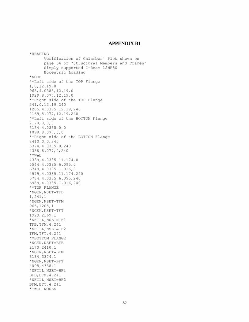
APPENDIX B1
*HEADING Verification of Galambos' Plot shown on page 64 of "Structural Members and Frames" Simply supported I-Beam 12WF50 Eccentric Loading *NODE **Left side of the TOP Flange 1,0,12.19,0 965,4.0385,12.19,0 1929,8.077,12.19,0 **Right side of the TOP Flange 241,0,12.19,240 1205,4.0385,12.19,240 2169,8.077,12.19,240 **Left side of the BOTTOM Flange 2170,0,0,0 3134,4.0385,0,0 4098,8.077,0,0 **Right side of the BOTTOM Flange 2410,0,0,240 3374,4.0385,0,240 4338,8.077,0,240 **Web 4339,4.0385,11.174,0 5544,4.0385,6.095,0 6749,4.0385,1.016,0 4579,4.0385,11.174,240 5784,4.0385,6.095,240 6989,4.0385,1.016,240 **TOP FLANGE *NGEN,NSET=TFB 1,241,1 *NGEN,NSET=TFM 965,1205,1 *NGEN,NSET=TFT 1929,2169,1 *NFILL,NSET=TF1 TFB,TFM,4,241 *NFILL,NSET=TF2 TFM,TFT,4,241 **BOTTOM FLANGE *NGEN,NSET=BFB 2170,2410,1 *NGEN,NSET=BFM 3134,3374,1 *NGEN,NSET=BFT 4098,4338,1 *NFILL,NSET=BF1 BFB,BFM,4,241 *NFILL,NSET=BF2 BFM,BFT,4,241 **WEB NODES
82

** *NGEN,NSET=WEBB 6749,6989,1 *NGEN,NSET=WEBM 5544,5784,1 *NGEN,NSET=WEBT 4339,4579,1 *NFILL,NSET=W1 WEBT,WEBM,5,241 *NFILL,NSET=W2 WEBM,WEBB,5,241 **NSET FOR BOUNDARY CONDITION *NSET,NSET=PINNED 5544 *NSET,NSET=ROLLER 5784 *NODE 6990,5.0385,6.095,120 ** **ELEMENT DEFINITIONS ** ** *ELEMENT,TYPE=S4R 1,1,2,243,242 *ELGEN,ELSET=TOPFLANGE 1,240,1,1,8,241,240 *ELEMENT,TYPE=S4R 1921,2170,2171,2412,2411 *ELGEN,ELSET=BOTTOMFLANGE 1921,240,1,1,8,241,240 *ELEMENT,TYPE=S4R 3841,965,966,4340,4339 *ELGEN,ELSET=WEBTOP 3841,240,1,1 *ELEMENT,TYPE=S4R 4081,4339,4340,4581,4580 *ELGEN,ELSET=WEBMIDDLE 4081,240,1,1,10,241,240 *ELEMENT,TYPE=S4R 6481,6749,6750,3135,3134 *ELGEN,ELSET=WEBBOTTOM 6481,240,1,1 **GROUPING ELEMENTS *ELSET,ELSET=WEB WEBTOP,WEBBOTTOM,WEBMIDDLE *ELEMENT,TYPE=B31,ELSET=LEVERARM 6722,5664,6990 *BEAM SECTION, SECTION=RECT, ELSET=LEVERARM, MATERIALS=RIGID 5.,5. *ELEMENT,TYPE=B31,ELSET=RIGIDBEAMTF 6723,121,362 6724,362,603 6725,603,844 6726,844,1085 6727,1085,1326
83

6728,1326,1567 6729,1567,1808 6730,1808,2049 *BEAM SECTION, SECTION=RECT,ELSET=RIGIDBEAMTF, MATERIALS=RIGID 5.,5. *ELEMENT,TYPE=B31,ELSET=RIGIDBEAMBF 6731,2290,2531 6732,2531,2772 6733,2772,3013 6734,3013,3254 6735,3254,3495 6736,3495,3736 6737,3736,3977 6738,3977,4218 *BEAM SECTION, SECTION=RECT,ELSET=RIGIDBEAMBF, MATERIALS=RIGID 5.,5. *ELEMENT,TYPE=B31,ELSET=RIGIDBEAMWEB 6739,1085,4459 6740,4459,4700 6741,4700,4941 6742,4941,5182 6743,5182,5423 6744,5423,5664 6745,5664,5905 6746,5905,6146 6747,6146,6387 6748,6387,6628 6749,6628,6869 6750,6869,3254 *ELEMENT, TYPE=B31,ELSET=RIGIDBEAMLEFT 6751,3374,6989 6752,6989,6748 6753,6748,6507 6754,6507,6266 6755,6266,6025 6756,6025,5784 6757,5784,5543 6758,5543,5302 6759,5302,5061 6760,5061,4820 6761,4820,4579 6762,4579,1205 *BEAM SECTION, SECTION=RECT,ELSET=RIGIDBEAMLEFT, MATERIALS=RIGID 5.,5. *ELEMENT,TYPE=B31,ELSET=RIGIDBEAMRIGHT 6763,3134,6749 6764,6749,6508 6765,6508,6267 6766,6267,6026 6767,6026,5785 6768,5785,5544 6769,5544,5303 6770,5303,5062 6771,5062,4821 6772,4821,4580 6773,4580,4339
84

6774,4339,965 *BEAM SECTION, SECTION=RECT,ELSET=RIGIDBEAMRIGHT, MATERIALS=RIGID 5.,5. *NSET, NSET=OUTPUT, GENERATE 965,1205,1 3134,3374,1 *BEAM SECTION, SECTION=RECT,ELSET=RIGIDBEAMWEB, MATERIALS=RIGID 5.,5. **MATERIAL PROPERTIES *SHELL SECTION,MATERIAL=STEEL,ELSET=TOPFLANGE 0.641 *SHELL SECTION,MATERIAL=STEEL,ELSET=BOTTOMFLANGE 0.641 *SHELL SECTION,MATERIAL=STEEL,ELSET=WEB 0.371 *MATERIAL,NAME=STEEL *ELASTIC 29500,0.3 *MATERIAL, NAME=RIGID *ELASTIC 295000,0.3 *BOUNDARY PINNED,1 PINNED,2 PINNED,3 PINNED,6 ROLLER,1 ROLLER,2 ROLLER,6 *STEP *STATIC *CLOAD 6990,2,-1 *ELPRINT,FREQUENCY=0 *NODE PRINT,FREQUENCY=1,NSET=OUTPUT U *END STEP
85

APPENDIX B2
*HEADING Linearized-eigenvalue Buckling Analysis Simply supported 12WF50 with Uniform Moment Applied *NODE **Left side of the TOP Flange 1,0,12.19,0 965,4.0385,12.19,0 1929,8.077,12.19,0 **Right side of the TOP Flange 241,0,12.19,240 1205,4.0385,12.19,240 2169,8.077,12.19,240 **Left side of the BOTTOM Flange 2170,0,0,0 3134,4.0385,0,0 4098,8.077,0,0 **Right side of the BOTTOM Flange 2410,0,0,240 3374,4.0385,0,240 4338,8.077,0,240 **Web 4339,4.0385,11.174,0 5544,4.0385,6.095,0 6749,4.0385,1.016,0 4579,4.0385,11.174,240 5784,4.0385,6.095,240 6989,4.0385,1.016,240 ** **TOP FLANGE ** *NGEN,NSET=TFB 1,241,1 *NGEN,NSET=TFM 965,1205,1 *NGEN,NSET=TFT 1929,2169,1 *NFILL,NSET=TF1 TFB,TFM,4,241 *NFILL,NSET=TF2 TFM,TFT,4,241 **BOTTOM FLANGE *NGEN,NSET=BFB 2170,2410,1 *NGEN,NSET=BFM 3134,3374,1 *NGEN,NSET=BFT 4098,4338,1 *NFILL,NSET=BF1 BFB,BFM,4,241 *NFILL,NSET=BF2 BFM,BFT,4,241
86

** **WEB NODES ** *NGEN,NSET=WEBB 6749,6989,1 *NGEN,NSET=WEBM 5544,5784,1 *NGEN,NSET=WEBT 4339,4579,1 *NFILL,NSET=W1 WEBT,WEBM,5,241 *NFILL,NSET=W2 WEBM,WEBB,5,241 **NSET FOR BOUNDARY CONDITION *NSET,NSET=PINNED 5544 *NSET,NSET=ROLLER 5784 ** **ELEMENT DEFINITIONS ** ** *ELEMENT,TYPE=S4R 1,1,2,243,242 *ELGEN,ELSET=TOPFLANGE 1,240,1,1,8,241,240 *ELEMENT,TYPE=S4R 1921,2170,2171,2412,2411 *ELGEN,ELSET=BOTTOMFLANGE 1921,240,1,1,8,241,240 *ELEMENT,TYPE=S4R 3841,965,966,4340,4339 *ELGEN,ELSET=WEBTOP 3841,240,1,1 *ELEMENT,TYPE=S4R 4081,4339,4340,4581,4580 *ELGEN,ELSET=WEBMIDDLE 4081,240,1,1,10,241,240 *ELEMENT,TYPE=S4R 6481,6749,6750,3135,3134 *ELGEN,ELSET=WEBBOTTOM 6481,240,1,1 **GROUPING ELEMENTS *ELSET,ELSET=WEB WEBTOP,WEBBOTTOM,WEBMIDDLE *ELEMENT, TYPE=B31,ELSET=RIGIDBEAMLEFT 6751,3374,6989 6752,6989,6748 6753,6748,6507 6754,6507,6266 6755,6266,6025 6756,6025,5784 6757,5784,5543 6758,5543,5302 6759,5302,5061 6760,5061,4820 6761,4820,4579
87
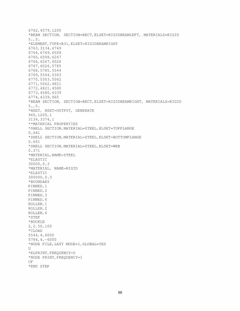
6762,4579,1205 *BEAM SECTION, SECTION=RECT,ELSET=RIGIDBEAMLEFT, MATERIALS=RIGID 5.,5. *ELEMENT,TYPE=B31,ELSET=RIGIDBEAMRIGHT 6763,3134,6749 6764,6749,6508 6765,6508,6267 6766,6267,6026 6767,6026,5785 6768,5785,5544 6769,5544,5303 6770,5303,5062 6771,5062,4821 6772,4821,4580 6773,4580,4339 6774,4339,965 *BEAM SECTION, SECTION=RECT,ELSET=RIGIDBEAMRIGHT, MATERIALS=RIGID 5.,5. *NSET, NSET=OUTPUT, GENERATE 965,1205,1 3134,3374,1 **MATERIAL PROPERTIES *SHELL SECTION,MATERIAL=STEEL,ELSET=TOPFLANGE 0.641 *SHELL SECTION,MATERIAL=STEEL,ELSET=BOTTOMFLANGE 0.641 *SHELL SECTION,MATERIAL=STEEL,ELSET=WEB 0.371 *MATERIAL,NAME=STEEL *ELASTIC 30000,0.3 *MATERIAL, NAME=RIGID *ELASTIC 300000,0.3 *BOUNDARY PINNED,1 PINNED,2 PINNED,3 PINNED,6 ROLLER,1 ROLLER,2 ROLLER,6 *STEP *BUCKLE 2,2,50,100 *CLOAD 5544,4,6000 5784,4,-6000 *NODE FILE,LAST MODE=1,GLOBAL=YES U *ELPRINT,FREQUENCY=0 *NODE PRINT,FREQUENCY=1 CF *END STEP
88

APPENDIX B3
*HEADING Simply supported 12WF50 with Uniform Moment applied to each end Compared to Eqn. 3.32 on Page 91 of "Structural Members and Frames" *NODE **Left side of the TOP Flange 1,0,12.19,0 965,4.0385,12.19,0 1929,8.077,12.19,0 **Right side of the TOP Flange 241,0,12.19,240 1205,4.0385,12.19,240 2169,8.077,12.19,240 **Left side of the BOTTOM Flange 2170,0,0,0 3134,4.0385,0,0 4098,8.077,0,0 **Right side of the BOTTOM Flange 2410,0,0,240 3374,4.0385,0,240 4338,8.077,0,240 **Web 4339,4.0385,11.174,0 5544,4.0385,6.095,0 6749,4.0385,1.016,0 4579,4.0385,11.174,240 5784,4.0385,6.095,240 6989,4.0385,1.016,240 ** **TOP FLANGE ** *NGEN,NSET=TFB 1,241,1 *NGEN,NSET=TFM 965,1205,1 *NGEN,NSET=TFT 1929,2169,1 *NFILL,NSET=TF1 TFB,TFM,4,241 *NFILL,NSET=TF2 TFM,TFT,4,241 **BOTTOM FLANGE *NGEN,NSET=BFB 2170,2410,1 *NGEN,NSET=BFM 3134,3374,1 *NGEN,NSET=BFT 4098,4338,1 *NFILL,NSET=BF1 BFB,BFM,4,241 *NFILL,NSET=BF2 BFM,BFT,4,241 **
89

**WEB NODES ** *NGEN,NSET=WEBB 6749,6989,1 *NGEN,NSET=WEBM 5544,5784,1 *NGEN,NSET=WEBT 4339,4579,1 *NFILL,NSET=W1 WEBT,WEBM,5,241 *NFILL,NSET=W2 WEBM,WEBB,5,241 **NSET FOR BOUNDARY CONDITION *NSET,NSET=PINNED 5544 *NSET,NSET=ROLLER 5784 ** **ELEMENT DEFINITIONS ** ** *ELEMENT,TYPE=S4R 1,1,2,243,242 *ELGEN,ELSET=TOPFLANGE 1,240,1,1,8,241,240 *ELEMENT,TYPE=S4R 1921,2170,2171,2412,2411 *ELGEN,ELSET=BOTTOMFLANGE 1921,240,1,1,8,241,240 *ELEMENT,TYPE=S4R 3841,965,966,4340,4339 *ELGEN,ELSET=WEBTOP 3841,240,1,1 *ELEMENT,TYPE=S4R 4081,4339,4340,4581,4580 *ELGEN,ELSET=WEBMIDDLE 4081,240,1,1,10,241,240 *ELEMENT,TYPE=S4R 6481,6749,6750,3135,3134 *ELGEN,ELSET=WEBBOTTOM 6481,240,1,1 **GROUPING ELEMENTS *ELSET,ELSET=WEB WEBTOP,WEBBOTTOM,WEBMIDDLE *ELEMENT, TYPE=B31,ELSET=RIGIDBEAMLEFT 6751,3374,6989 6752,6989,6748 6753,6748,6507 6754,6507,6266 6755,6266,6025 6756,6025,5784 6757,5784,5543 6758,5543,5302 6759,5302,5061 6760,5061,4820 6761,4820,4579 6762,4579,1205
90

*BEAM SECTION, SECTION=RECT,ELSET=RIGIDBEAMLEFT, MATERIALS=RIGID 5.,5. *ELEMENT,TYPE=B31,ELSET=RIGIDBEAMRIGHT 6763,3134,6749 6764,6749,6508 6765,6508,6267 6766,6267,6026 6767,6026,5785 6768,5785,5544 6769,5544,5303 6770,5303,5062 6771,5062,4821 6772,4821,4580 6773,4580,4339 6774,4339,965 *BEAM SECTION, SECTION=RECT,ELSET=RIGIDBEAMRIGHT, MATERIALS=RIGID 5.,5. *NSET, NSET=OUTPUT, GENERATE 965,1205,1 3134,3374,1 **MATERIAL PROPERTIES *SHELL SECTION,MATERIAL=STEEL,ELSET=TOPFLANGE 0.641 *SHELL SECTION,MATERIAL=STEEL,ELSET=BOTTOMFLANGE 0.641 *SHELL SECTION,MATERIAL=STEEL,ELSET=WEB 0.371 *MATERIAL,NAME=STEEL *ELASTIC 30000,0.3 *MATERIAL, NAME=RIGID *ELASTIC 300000,0.3 *BOUNDARY PINNED,1 PINNED,2 PINNED,3 PINNED,6 ROLLER,1 ROLLER,2 ROLLER,6 *STEP,NLGEOM,INC=30 *STATIC,RIKS 0.01,1.,0.0000000001 *CLOAD 5544,4,6000 5784,4,-6000 *ELPRINT,FREQUENCY=0 *NODE PRINT,FREQUENCY=1,NSET=OUTPUT U *END STEP
91

APPENDIX B4
*Heading Cruciform Cross-section Linearized-eigenvalue Buckling Analysis Axial Compressive Loading *NODE **BOTTOM 1ST FLANGE 1,9,0,0 724,12,0,0 1447,15,0,0 **TOP 1ST FLANGE 241,9,240,0 964,12,240,0 1687,15,240,0 **BOTTOM 2ND FLANGE 1688,0,0,9 2411,0,0,12 3134,0,0,15 **TOP 2ND FLANGE 1928,0,240,9 2651,0,240,12 3374,0,240,15 **BOTTOM 3RD FLANGE 3375,9,0,24 4098,12,0,24 4821,15,0,24 **TOP 3RD FLANGE 3615,9,240,24 4338,12,240,24 5061,15,240,24 **BOTTOM 4TH FLANGE 5062,24,0,9 5785,24,0,12 6508,24,0,15 **TOP 4TH FLANGE 5302,24,240,9 6025,24,240,12 6748,24,240,15 **WEB 1 6749,12,0,1 6869,12,120,1 6989,12,240,1 9400,12,0,12 9520,12,120,12 9640,12,240,12 12051,12,0,23 12171,12,120,23 12291,12,240,23 **WEB 2 12300,1,0,12 12540,1,240,12 14710,11,0,12 14950,11,240,12 16000,13,0,12
92

16240,13,240,12 18410,23,0,12 18650,23,240,12 ** **1ST FLANGE ** *NGEN,NSET=R1 1,241,1 *NGEN,NSET=M1 724,964,1 *NGEN,NSET=L1 1447,1687,1 *NFILL,NSET=O1 R1,M1,3,241 *NFILL,NSET=O2 M1,L1,3,241 ** **2ND FLANGE ** *NGEN,NSET=R2 1688,1928,1 *NGEN,NSET=M2 2411,2651,1 *NGEN,NSET=L2 3134,3374,1 *NFILL,NSET=T1 R2,M2,3,241 *NFILL,NSET=T2 M2,L2,3,241 ** **3RD FLANGE ** *NGEN,NSET=R3 3375,3615,1 *NGEN,NSET=M3 4098,4338,1 *NGEN,NSET=L3 4821,5061,1 *NFILL,NSET=TH1 R3,M3,3,241 *NFILL,NSET=TH2 M3,L3,3,241 ** **4TH FLANGE ** *NGEN,NSET=R4 5062,5302,1 *NGEN,NSET=M4 5785,6025,1 *NGEN,NSET=L4 6508,6748,1 *NFILL,NSET=F1 R4,M4,3,241 *NFILL,NSET=F2 M4,L4,3,241 **
93

**WEB 1 ** *NGEN,NSET=WEB1L 6749,6989,1 *NGEN,NSET=WEB1M 9400,9640,1 *NGEN,NSET=WEB1R 12051,12291,1 *NFILL,NSET=WEB11 WEB1L,WEB1M,11,241 *NFILL,NSET=WEB12 WEB1M,WEB1R,11,241 ** **WEB 2 ** *NGEN,NSET=WEB2R 12300,12540,1 *NGEN,NSET=WEB2M1 14710,14950,1 *NGEN,NSET=WEB2M2 16000,16240,1 *NGEN,NSET=WEB2L 18410,18650,1 *NFILL,NSET=WEB21 WEB2R,WEB2M1,10,241 *NFILL,NSET=WEB22 WEB2M2,WEB2L,10,241 ** **BOUNDARY CONDITIONS ** *NSET,NSET=PINNED 9400 *NSET,NSET=ROLLER 9640 ** **ELEMENT DEFINITIONS ** *ELEMENT,TYPE=S4R 1,1,2,243,242 *ELGEN,ELSET=FLANGE1 1,240,1,1,6,241,240 ** *ELEMENT,TYPE=S4R 1441,1688,1689,1930,1929 *ELGEN,ELSET=FLANGE2 1441,240,1,1,6,241,240 ** *ELEMENT,TYPE=S4R 2881,3375,3376,3617,3616 *ELGEN,ELSET=FLANGE3 2881,240,1,1,6,241,240 ** *ELEMENT,TYPE=S4R 4321,5062,5063,5304,5303 *ELGEN,ELSET=FLANGE4 4321,240,1,1,6,241,240 **
94

*ELEMENT,TYPE=S4R 5761,724,725,6750,6749 *ELGEN,ELSET=WEB111 5761,240,1,1 ** *ELEMENT,TYPE=S4R 6001,6749,6750,6991,6990 *ELGEN,ELSET=WEB112 6001,240,1,1,22,241,240 ** *ELEMENT,TYPE=S4R 11281,12051,12052,4099,4098 *ELGEN,ELSET=WEB113 11281,240,1,1 ** *ELSET,ELSET=WEB1 WEB111,WEB112,WEB113 ** *ELEMENT,TYPE=S4R 11600,2411,2412,12301,12300 *ELGEN,ELSET=WEB2R1 11600,240,1,1 ** *ELEMENT,TYPE=S4R 11841,12300,12301,12542,12541 *ELGEN,ELSET=WEB2R2 11841,240,1,1,10,241,240 ** *ELEMENT,TYPE=S4R 14241,14710,14711,9401,9400 *ELGEN,ELSET=WEB2M1 14241,240,1,1 ** *ELEMENT,TYPE=S4R 14481,9400,9401,16001,16000 *ELGEN,ELSET=WEB2M2 14481,240,1,1 ** *ELEMENT,TYPE=S4R 14721,16000,16001,16242,16241 *ELGEN,ELSET=WEB2L1 14721,240,1,1,10,241,240 ** *ELEMENT,TYPE=S4R 17121,18410,18411,5786,5785 *ELGEN,ELSET=WEB2L2 17121,240,1,1 ** *ELSET,ELSET=WEB2 WEB2R1,WEB2R2,WEB2M1,WEB2M2,WEB2L1,WEB2L2 ** ** *ELEMENT, TYPE=B31,ELSET=RIGIDTOP1 18000,964,6989 18001,6989,7230 18003,7230,7471 18004,7471,7712
95

18005,7712,7953 18006,7953,8194 18007,8194,8435 18008,8435,8676 18009,8676,8917 18010,8917,9158 18011,9158,9399 18012,9399,9640 18013,9640,9881 18014,9881,10122 18015,10122,10363 18016,10363,10604 18017,10604,10845 18018,10845,11086 18019,11086,11327 18020,11327,11568 18021,11568,11809 18022,11809,12050 18023,12050,12291 18024,12291,4338 *BEAM SECTION, SECTION=RECT,ELSET=RIGIDTOP1, MATERIALS=RIGID 5.,5. 0,-1,0 *ELEMENT,TYPE=B31,ELSET=RIGIDBOTTOM1 18025,724,6749 18026,6749,6990 18027,6990,7231 18028,7231,7472 18029,7472,7713 18030,7713,7954 18031,7954,8195 18032,8195,8436 18033,8436,8677 18034,8677,8918 18035,8918,9159 18036,9159,9400 18037,9400,9641 18038,9641,9882 18039,9882,10123 18040,10123,10364 18041,10364,10605 18042,10605,10846 18043,10846,11087 18044,11087,11328 18045,11328,11569 18046,11569,11810 18047,11810,12051 18048,12051,4098 *BEAM SECTION, SECTION=RECT,ELSET=RIGIDBOTTOM1, MATERIALS=RIGID 5.,5. 0,-1,0 *ELEMENT, TYPE=B31,ELSET=RIGIDTOP2 18049,2651,12540 18050,12540,12781 18051,12781,13022 18052,13022,13263 18053,13263,13504
96

18054,13504,13745 18055,13745,13986 18056,13986,14227 18057,14227,14468 18058,14468,14709 18059,14709,14950 18060,14950,9640 18061,9640,16240 18062,16240,16481 18063,16481,16722 18064,16722,16963 18065,16963,17204 18066,17204,17445 18067,17445,17686 18068,17686,17927 18069,17927,18168 18070,18168,18409 18071,18409,18650 18072,18650,6025 *BEAM SECTION, SECTION=RECT,ELSET=RIGIDTOP2, MATERIALS=RIGID 5.,5. 0,-1,0 *ELEMENT,TYPE=B31,ELSET=RIGIDBOTTOM2 18073,2411,12300 18074,12300,12541 18075,12541,12782 18076,12782,13023 18077,13023,13264 18078,13264,13505 18079,13505,13746 18080,13746,13987 18081,13987,14228 18082,14228,14469 18083,14469,14710 18084,14710,9400 18085,9400,16000 18086,16000,16241 18087,16241,16482 18088,16482,16723 18089,16723,16964 18090,16964,17205 18091,17205,17446 18092,17446,17687 18093,17687,17928 18094,17928,18169 18095,18169,18410 18096,18410,5785 *BEAM SECTION, SECTION=RECT,ELSET=RIGIDBOTTOM2, MATERIALS=RIGID 5.,5. 0,-1,0 ** ** **MATERIAL PROPERTIES ** *SHELL SECTION,MATERIAL=STEEL,ELSET=FLANGE1 0.25 *SHELL SECTION,MATERIAL=STEEL,ELSET=FLANGE2
97
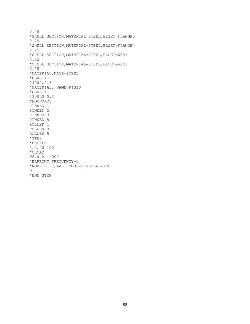
0.25 *SHELL SECTION,MATERIAL=STEEL,ELSET=FLANGE3 0.25 *SHELL SECTION,MATERIAL=STEEL,ELSET=FLANGE4 0.25 *SHELL SECTION,MATERIAL=STEEL,ELSET=WEB1 0.25 *SHELL SECTION,MATERIAL=STEEL,ELSET=WEB2 0.25 *MATERIAL,NAME=STEEL *ELASTIC 29000,0.3 *MATERIAL, NAME=RIGID *ELASTIC 290000,0.3 *BOUNDARY PINNED,1 PINNED,2 PINNED,3 PINNED,5 ROLLER,1 ROLLER,3 ROLLER,5 *STEP *BUCKLE 5,5,50,100 *CLOAD 9640,2,-1000 *ELPRINT,FREQUENCY=0 *NODE FILE,LAST MODE=1,GLOBAL=YES U *END STEP
98

APPENDIX B5
*Heading Postbuckling Analysis of Cruciform Column Axial Compressive Load Scale Factor=L/1000 *NODE **BOTTOM 1ST FLANGE 1,9,0,0 724,12,0,0 1447,15,0,0 **TOP 1ST FLANGE 241,9,240,0 964,12,240,0 1687,15,240,0 **BOTTOM 2ND FLANGE 1688,0,0,9 2411,0,0,12 3134,0,0,15 **TOP 2ND FLANGE 1928,0,240,9 2651,0,240,12 3374,0,240,15 **BOTTOM 3RD FLANGE 3375,9,0,24 4098,12,0,24 4821,15,0,24 **TOP 3RD FLANGE 3615,9,240,24 4338,12,240,24 5061,15,240,24 **BOTTOM 4TH FLANGE 5062,24,0,9 5785,24,0,12 6508,24,0,15 **TOP 4TH FLANGE 5302,24,240,9 6025,24,240,12 6748,24,240,15 **WEB 1 6749,12,0,1 6869,12,120,1 6989,12,240,1 9400,12,0,12 9520,12,120,12 9640,12,240,12 12051,12,0,23 12171,12,120,23 12291,12,240,23 **WEB 2 12300,1,0,12 12540,1,240,12 14710,11,0,12 14950,11,240,12 16000,13,0,12
99

16240,13,240,12 18410,23,0,12 18650,23,240,12 ** **1ST FLANGE ** *NGEN,NSET=R1 1,241,1 *NGEN,NSET=M1 724,964,1 *NGEN,NSET=L1 1447,1687,1 *NFILL,NSET=O1 R1,M1,3,241 *NFILL,NSET=O2 M1,L1,3,241 ** **2ND FLANGE ** *NGEN,NSET=R2 1688,1928,1 *NGEN,NSET=M2 2411,2651,1 *NGEN,NSET=L2 3134,3374,1 *NFILL,NSET=T1 R2,M2,3,241 *NFILL,NSET=T2 M2,L2,3,241 ** **3RD FLANGE ** *NGEN,NSET=R3 3375,3615,1 *NGEN,NSET=M3 4098,4338,1 *NGEN,NSET=L3 4821,5061,1 *NFILL,NSET=TH1 R3,M3,3,241 *NFILL,NSET=TH2 M3,L3,3,241 ** **4TH FLANGE ** *NGEN,NSET=R4 5062,5302,1 *NGEN,NSET=M4 5785,6025,1 *NGEN,NSET=L4 6508,6748,1 *NFILL,NSET=F1 R4,M4,3,241 *NFILL,NSET=F2 M4,L4,3,241 **
100

**WEB 1 ** *NGEN,NSET=WEB1L 6749,6989,1 *NGEN,NSET=WEB1M 9400,9640,1 *NGEN,NSET=WEB1R 12051,12291,1 *NFILL,NSET=WEB11 WEB1L,WEB1M,11,241 *NFILL,NSET=WEB12 WEB1M,WEB1R,11,241 ** **WEB 2 ** *NGEN,NSET=WEB2R 12300,12540,1 *NGEN,NSET=WEB2M1 14710,14950,1 *NGEN,NSET=WEB2M2 16000,16240,1 *NGEN,NSET=WEB2L 18410,18650,1 *NFILL,NSET=WEB21 WEB2R,WEB2M1,10,241 *NFILL,NSET=WEB22 WEB2M2,WEB2L,10,241 ** **BOUNDARY CONDITIONS ** *NSET,NSET=PINNED 9400 *NSET,NSET=ROLLER 9640 ** **ELEMENT DEFINITIONS ** *ELEMENT,TYPE=S4R 1,1,2,243,242 *ELGEN,ELSET=FLANGE1 1,240,1,1,6,241,240 ** *ELEMENT,TYPE=S4R 1441,1688,1689,1930,1929 *ELGEN,ELSET=FLANGE2 1441,240,1,1,6,241,240 ** *ELEMENT,TYPE=S4R 2881,3375,3376,3617,3616 *ELGEN,ELSET=FLANGE3 2881,240,1,1,6,241,240 ** *ELEMENT,TYPE=S4R 4321,5062,5063,5304,5303 *ELGEN,ELSET=FLANGE4 4321,240,1,1,6,241,240 **
101

*ELEMENT,TYPE=S4R 5761,724,725,6750,6749 *ELGEN,ELSET=WEB111 5761,240,1,1 ** *ELEMENT,TYPE=S4R 6001,6749,6750,6991,6990 *ELGEN,ELSET=WEB112 6001,240,1,1,22,241,240 ** *ELEMENT,TYPE=S4R 11281,12051,12052,4099,4098 *ELGEN,ELSET=WEB113 11281,240,1,1 ** *ELSET,ELSET=WEB1 WEB111,WEB112,WEB113 ** *ELEMENT,TYPE=S4R 11600,2411,2412,12301,12300 *ELGEN,ELSET=WEB2R1 11600,240,1,1 ** *ELEMENT,TYPE=S4R 11841,12300,12301,12542,12541 *ELGEN,ELSET=WEB2R2 11841,240,1,1,10,241,240 ** *ELEMENT,TYPE=S4R 14241,14710,14711,9401,9400 *ELGEN,ELSET=WEB2M1 14241,240,1,1 ** *ELEMENT,TYPE=S4R 14481,9400,9401,16001,16000 *ELGEN,ELSET=WEB2M2 14481,240,1,1 ** *ELEMENT,TYPE=S4R 14721,16000,16001,16242,16241 *ELGEN,ELSET=WEB2L1 14721,240,1,1,10,241,240 ** *ELEMENT,TYPE=S4R 17121,18410,18411,5786,5785 *ELGEN,ELSET=WEB2L2 17121,240,1,1 ** *ELSET,ELSET=WEB2 WEB2R1,WEB2R2,WEB2M1,WEB2M2,WEB2L1,WEB2L2 ** ** *ELEMENT, TYPE=B31,ELSET=RIGIDTOP1 18000,964,6989 18001,6989,7230 18003,7230,7471 18004,7471,7712
102

18005,7712,7953 18006,7953,8194 18007,8194,8435 18008,8435,8676 18009,8676,8917 18010,8917,9158 18011,9158,9399 18012,9399,9640 18013,9640,9881 18014,9881,10122 18015,10122,10363 18016,10363,10604 18017,10604,10845 18018,10845,11086 18019,11086,11327 18020,11327,11568 18021,11568,11809 18022,11809,12050 18023,12050,12291 18024,12291,4338 *BEAM SECTION, SECTION=RECT,ELSET=RIGIDTOP1, MATERIALS=RIGID 5.,5. 0,-1,0 *ELEMENT,TYPE=B31,ELSET=RIGIDBOTTOM1 18025,724,6749 18026,6749,6990 18027,6990,7231 18028,7231,7472 18029,7472,7713 18030,7713,7954 18031,7954,8195 18032,8195,8436 18033,8436,8677 18034,8677,8918 18035,8918,9159 18036,9159,9400 18037,9400,9641 18038,9641,9882 18039,9882,10123 18040,10123,10364 18041,10364,10605 18042,10605,10846 18043,10846,11087 18044,11087,11328 18045,11328,11569 18046,11569,11810 18047,11810,12051 18048,12051,4098 *BEAM SECTION, SECTION=RECT,ELSET=RIGIDBOTTOM1, MATERIALS=RIGID 5.,5. 0,-1,0 *ELEMENT, TYPE=B31,ELSET=RIGIDTOP2 18049,2651,12540 18050,12540,12781 18051,12781,13022 18052,13022,13263 18053,13263,13504
103

18054,13504,13745 18055,13745,13986 18056,13986,14227 18057,14227,14468 18058,14468,14709 18059,14709,14950 18060,14950,9640 18061,9640,16240 18062,16240,16481 18063,16481,16722 18064,16722,16963 18065,16963,17204 18066,17204,17445 18067,17445,17686 18068,17686,17927 18069,17927,18168 18070,18168,18409 18071,18409,18650 18072,18650,6025 *BEAM SECTION, SECTION=RECT,ELSET=RIGIDTOP2, MATERIALS=RIGID 5.,5. 0,-1,0 *ELEMENT,TYPE=B31,ELSET=RIGIDBOTTOM2 18073,2411,12300 18074,12300,12541 18075,12541,12782 18076,12782,13023 18077,13023,13264 18078,13264,13505 18079,13505,13746 18080,13746,13987 18081,13987,14228 18082,14228,14469 18083,14469,14710 18084,14710,9400 18085,9400,16000 18086,16000,16241 18087,16241,16482 18088,16482,16723 18089,16723,16964 18090,16964,17205 18091,17205,17446 18092,17446,17687 18093,17687,17928 18094,17928,18169 18095,18169,18410 18096,18410,5785 *BEAM SECTION, SECTION=RECT,ELSET=RIGIDBOTTOM2, MATERIALS=RIGID 5.,5. 0,-1,0 ** ** **MATERIAL PROPERTIES ** *SHELL SECTION,MATERIAL=STEEL,ELSET=FLANGE1 0.25 *SHELL SECTION,MATERIAL=STEEL,ELSET=FLANGE2
104
0.25 *SHELL SECTION,MATERIAL=STEEL,ELSET=FLANGE3 0.25 *SHELL SECTION,MATERIAL=STEEL,ELSET=FLANGE4 0.25 *SHELL SECTION,MATERIAL=STEEL,ELSET=WEB1 0.25 *SHELL SECTION,MATERIAL=STEEL,ELSET=WEB2 0.25 *MATERIAL,NAME=STEEL *ELASTIC 29000,0.3 *MATERIAL, NAME=RIGID *ELASTIC 290000,0.3 *IMPERFECTION, FILE=Cruc3LEBimp, STEP=1 1,0.24 *BOUNDARY PINNED,1 PINNED,2 PINNED,3 PINNED,5 ROLLER,1 ROLLER,3 ROLLER,5 *STEP,NLGEOM,INC=30 *STATIC,RIKS 0.01,1.,0.0000000001 *CLOAD 9640,2,-100 *EL PRINT,FREQUENCY=16,ELSET=FLANGE1 S *NODE PRINT,FREQUENCY=16 UR3 *END STEP
105

APPENDIX B6
*Heading Tee-shaped Column with Eccentric Loading Linearized-eigenvalue Buckling Analysis *NODE **BOTTOM OF FLANGE 1,0,0,0 280,2.01,0,0 559,4.02,0,0 **TOP OF FLANGE 93,0,91.42,0 372,2.01,91.42,0 651,4.02,91.42,0 **BOTTOM OF WEB 700,2.01,0,0.152 793,2.01,0,1.3705 886,2.01,0,2.52 1165,2.01,0,4.912 **TOP OF WEB 792,2.01,91.42,0.152 885,2.01,91.42,1.3705 978,2.01,91.42,2.52 1257,2.01,91.42,4.912 ** **NODE SETS ** **FLANGE ** *NGEN,NSET=FLL 1,93,1 *NGEN,NSET=FLM 280,372,1 *NGEN,NSET=FLR 559,651,1 *NFILL,NSET=FLANGE1 FLL,FLM,3,93 *NFILL,NSET=FLANGE2 FLM,FLR,3,93 ** **WEB ** *NGEN,NSET=WEB1 700,792,1 *NGEN,NSET=WEB2 886,978,1 *NFILL,NSET=WEB4 WEB1,WEB2,2,93 *NGEN,NSET=WEB3 1165,1257,1 *NFILL,NSET=WEB5 WEB2,WEB3,3,93 ** **BC'S
106

** *NSET,NSET=PINNED 793 *NSET,NSET=ROLLER 885 ** **ELEMENT DEFINITIONS ** *ELEMENT,TYPE=S4R 1,1,2,95,94 *ELGEN,ELSET=FLANGE1 1,92,1,1,3,93,92 *ELEMENT,TYPE=S4R 277,280,281,374,373 *ELGEN,ELSET=FLANGE2 277,92,1,1,3,93,92 ** *ELEMENT,TYPE=S4R 553,280,281,701,700 *ELGEN,ELSET=WEB1 553,92,1,1 ** *ELEMENT,TYPE=S4R 645,700,701,794,793 *ELGEN,ELSET=WEB2 645,92,1,1,2,93,92 ** *ELEMENT,TYPE=S4R 829,886,887,980,979 *ELGEN,ELSET=WEB3 829,92,1,1,3,93,92 ** *ELSET,ELSET=WEB WEB1,WEB2,WEB3 ** *ELEMENT, TYPE=B31,ELSET=RIGIDTOPFLANGE 1106,93,186 1107,186,279 1108,279,372 1109,372,465 1110,465,558 1111,558,651 *BEAM SECTION, SECTION=RECT,ELSET=RIGIDTOPFLANGE, MATERIALS=RIGID 5.,5. 0,-1,0 *ELEMENT, TYPE=B31,ELSET=RIGIDBOTTOMFLANGE 1112,1,94 1113,94,187 1114,187,280 1115,280,373 1116,373,466 1117,466,559 *BEAM SECTION, SECTION=RECT,ELSET=RIGIDBOTTOMFLANGE, MATERIALS=RIGID 5.,5. *ELEMENT, TYPE=B31,ELSET=RIGIDTOPWEB 1118,372,792 1119,792,885
107

1120,885,978 1121,978,1071 1122,1071,1164 1123,1164,1257 *BEAM SECTION, SECTION=RECT,ELSET=RIGIDTOPWEB, MATERIALS=RIGID 5.,5. 0,-1,0 ** *ELEMENT, TYPE=B31,ELSET=RIGIDBOTTOMWEB 1124,280,700 1125,700,793 1126,793,886 1127,886,979 1128,979,1072 1129,1072,1165 *BEAM SECTION, SECTION=RECT,ELSET=RIGIDBOTTOMWEB, MATERIALS=RIGID 5.,5. 0,-1,0 ** ** **MATERIAL PROPERTIES ** *SHELL SECTION,MATERIAL=STEEL,ELSET=FLANGE1 0.303 *SHELL SECTION,MATERIAL=STEEL,ELSET=FLANGE2 0.303 *SHELL SECTION,MATERIAL=STEEL,ELSET=WEB 0.303 *MATERIAL,NAME=STEEL *ELASTIC 29000,0.3 *MATERIAL, NAME=RIGID *ELASTIC 290000,0.3 *BOUNDARY PINNED,1 PINNED,2 PINNED,3 PINNED,5 ROLLER,1 ROLLER,3 ROLLER,5 *STEP *BUCKLE 5,5,50,100 *CLOAD 1164,2,-1 *NODE FILE,LAST MODE=1,GLOBAL=YES U *END STEP
108

APPENDIX B7
*Heading Tee-shaped Column with Eccentric Loading Postbuckling Analysis Scale Factor =L/1000 *NODE **BOTTOM OF FLANGE 1,0,0,0 280,2.01,0,0 559,4.02,0,0 **TOP OF FLANGE 93,0,91.42,0 372,2.01,91.42,0 651,4.02,91.42,0 **BOTTOM OF WEB 700,2.01,0,0.152 793,2.01,0,1.3705 886,2.01,0,2.52 1165,2.01,0,4.912 **TOP OF WEB 792,2.01,91.42,0.152 885,2.01,91.42,1.3705 978,2.01,91.42,2.52 1257,2.01,91.42,4.912 ** **NODE SETS ** **FLANGE ** *NGEN,NSET=FLL 1,93,1 *NGEN,NSET=FLM 280,372,1 *NGEN,NSET=FLR 559,651,1 *NFILL,NSET=FLANGE1 FLL,FLM,3,93 *NFILL,NSET=FLANGE2 FLM,FLR,3,93 ** **WEB ** *NGEN,NSET=WEB1 700,792,1 *NGEN,NSET=WEB2 886,978,1 *NFILL,NSET=WEB4 WEB1,WEB2,2,93 *NGEN,NSET=WEB3 1165,1257,1 *NFILL,NSET=WEB5 WEB2,WEB3,3,93 ** **BC'S
109

** *NSET,NSET=PINNED 793 *NSET,NSET=ROLLER 885 ** **ELEMENT DEFINITIONS ** *ELEMENT,TYPE=S4R 1,1,2,95,94 *ELGEN,ELSET=FLANGE1 1,92,1,1,3,93,92 *ELEMENT,TYPE=S4R 277,280,281,374,373 *ELGEN,ELSET=FLANGE2 277,92,1,1,3,93,92 ** *ELEMENT,TYPE=S4R 553,280,281,701,700 *ELGEN,ELSET=WEB1 553,92,1,1 ** *ELEMENT,TYPE=S4R 645,700,701,794,793 *ELGEN,ELSET=WEB2 645,92,1,1,2,93,92 ** *ELEMENT,TYPE=S4R 829,886,887,980,979 *ELGEN,ELSET=WEB3 829,92,1,1,3,93,92 ** *ELSET,ELSET=WEB WEB1,WEB2,WEB3 ** *ELEMENT, TYPE=B31,ELSET=RIGIDTOPFLANGE 1106,93,186 1107,186,279 1108,279,372 1109,372,465 1110,465,558 1111,558,651 *BEAM SECTION, SECTION=RECT,ELSET=RIGIDTOPFLANGE, MATERIALS=RIGID 5.,5. 0,-1,0 *ELEMENT, TYPE=B31,ELSET=RIGIDBOTTOMFLANGE 1112,1,94 1113,94,187 1114,187,280 1115,280,373 1116,373,466 1117,466,559 *BEAM SECTION, SECTION=RECT,ELSET=RIGIDBOTTOMFLANGE, MATERIALS=RIGID 5.,5. *ELEMENT, TYPE=B31,ELSET=RIGIDTOPWEB 1118,372,792
110

1119,792,885 1120,885,978 1121,978,1071 1122,1071,1164 1123,1164,1257 *BEAM SECTION, SECTION=RECT,ELSET=RIGIDTOPWEB, MATERIALS=RIGID 5.,5. 0,-1,0 ** *ELEMENT, TYPE=B31,ELSET=RIGIDBOTTOMWEB 1124,280,700 1125,700,793 1126,793,886 1127,886,979 1128,979,1072 1129,1072,1165 *BEAM SECTION, SECTION=RECT,ELSET=RIGIDBOTTOMWEB, MATERIALS=RIGID 5.,5. 0,-1,0 ** **MATERIAL PROPERTIES ** *SHELL SECTION,MATERIAL=STEEL,ELSET=FLANGE1 0.303 *SHELL SECTION,MATERIAL=STEEL,ELSET=FLANGE2 0.303 *SHELL SECTION,MATERIAL=STEEL,ELSET=WEB 0.303 *MATERIAL,NAME=STEEL *ELASTIC 29000,0.3 *MATERIAL, NAME=RIGID *ELASTIC 290000,0.3 *IMPERFECTION,FILE=TeeIMP2, STEP=1 1,0.09142 *BOUNDARY PINNED,1 PINNED,2 PINNED,3 PINNED,5 ROLLER,1 ROLLER,3 ROLLER,5 *STEP,NLGEOM,INC=30 *STATIC,RIKS 0.01,1.,0.0000000001 *CLOAD 978,2,-10 *CLOAD 886,2,10 *EL PRINT,FREQ=11,ELSET=FLANGE1 S *EL PRINT,FREQ=11,ELSET=FLANGE2 S *NODE PRINT,FREQ=11 UR3
111
*END STEP
112

APPENDIX C
THEORETICAL RESULTS
Appendix C includes all calculations performed to arrive at theoretical results for this study. The
computations are presented in a MathCAD worksheet with cross-sections of each member
included. The results provided by these computations are used to compare with the finite
element analysis in order to prove or discount the validity of the Wagner Hypothesis. Appendix
C1 shows the calculations related to the simply supported 12WF50 section with a uniform
moment applied to each end of the beam. Appendix C2 illustrates the theoretical results
associated with the cruciform-shaped column. For this member there were equations presented
by Ojalvo for both the critical buckling load including the Wagner effect and the critical load
calculated without the use of the Wagner effect.
Appendix C3 demonstrates the theoretical equations used for the tee-shaped column.
This member was used due to the fact that experimental tests were performed on various tee-
shaped columns at the Xian Institute of Metallurgy and Construction Engineering in the late
1970’s. In this case, the finite element results could be compared to both the theoretical results
presented in Appendix C3 as well as the finite element results found in the ABAQUS modeling.
The equations used in these computations are specified by both Galambos and Ojalvo.
113

APPENDIX C1
Doubly Symmetric I-Beam Closed Form Solution presented in "Structural Members and Frames" page 59
** All measurements are in inches and kips
t
w
d
b
L 240:= G 11500:= E 30000:= Iw 1881:= w 0.371:=
Kt 1.82:= Iy 56.4:= Ix 394.5:= Sx 64.7:= Sw 30.18:=
d 12.19:= b 8.077:= t 0.641:= wn 23.32:=
λG Kt⋅
E Iw⋅:=
λ2
3.709 10 4−×= λ L⋅ 4.622=
Critical Moment:
n 1:=
Moπ n⋅L
E Iy⋅ G⋅ Kt⋅ 1n2
π2
⋅ E⋅ Iw⋅
G Kt⋅ L2⋅
+⎛⎜⎜⎝
⎞
⎠⋅⋅:= (Eqn. 3.32 on page 91)
Mo 2.978 103×= kip in⋅
Summary: Galambos Mcr = 248.2 kips ABAQUS Mcr = (6000 kips * 0.5025) = 251.25 kips
Mo12
248.206= kip ft⋅
114

APPENDIX C2
Cruciform Cross-section with Flanges Closed Form Solution presented in "Thin-Walled Open-Profile Bars" pages 145 and 147
** All measurements are in inches and kips
2d 2d
t2d
t0.5d
0.5d
2d
0.5d 0.5d
d 6:= t 0.25:= L 240:= E 29000:= ν 0.3:=
GE
2 1 ν+( )⋅:=
Critical Moment (including Wagner's Hypothesis):
32
23
2
2
0 2716
916)( td
LE
dtG
LEIGJ
IAP ππ
ωθ +=+= (Eqn. 16 on page 145)
P169
G⋅t3
d⋅
⎛⎜⎝
⎞
⎠1627
E⋅π
2
L2⋅ t⋅ d3
⋅+:=
P 210.648= kips
115

Critical Moment (excluding Wagner's Hypothesis):
32
23
2
22
2 43
49)}2{(4 Etd
LdtG
LdEIEIGJ
aP y
ππωθ +=++= (Eqn. 19 on page 147)
P94
G⋅t3
d⋅
⎛⎜⎝
⎞
⎠34
π2
L2⋅ E⋅ t⋅ d3⋅+:=
P 266.602= kips
Summary: Including Wagner Pcr = 210.65 kips Without Using Wagner Pcr = 266.60 kips ABAQUS Pcr = 206.75 kips
116

APPENDIX C3
Calculation of the critical buckling load of Chen's experimental specimen PD3-1 (Corrected eccentricity):
d 5.067:= tf 0.303:= tw 0.303:= h d tf−:= bf 4:=
Af bf tf⋅:= Aw h tw⋅:= A Af Aw+:= D dtf2
−:=
y1A
Af tf⋅
2Aw tf
h2
+⎛⎜⎝
⎞⎠
⋅+⎡⎢⎣
⎤⎥⎦
⋅:= y 1.529= ybar ytf2
−⎛⎜⎝
⎞⎠
1−⋅:= ybar 1.377−=
Ixbf tf 3⋅ h3 tw⋅+
12Af y
tf2
−⎛⎜⎝
⎞⎠
2⋅+ Aw tf
h2
+ y−⎛⎜⎝
⎞⎠
2⋅+:= Ix 6.968=
Iybf 3 tf⋅ h tw3⋅+
12:= Iy 1.627= ro ybar2 Ix Iy+
A+:=
H 1ybarro
⎛⎜⎝
⎞⎠
2−:= J
bf tf 3⋅ D tw3
⋅+
3:=
117

βx1Ix
tw4
D y−( )4 y tf−( )4−⎡⎣ ⎤⎦⋅ bf tf⋅ y
tf2
−⎛⎜⎝
⎞⎠
⋅bf 2
12y
tf2
−⎛⎜⎝
⎞⎠
2+
⎡⎢⎣
⎤⎥⎦
⋅−⎡⎢⎣
⎤⎥⎦
⋅ 2 ybar⋅−:=
root Py P−( ) ro2 Pz⋅ 1.15 P⋅ βx⋅− P ro2⋅−( )⋅ P ybar⋅ 1.15 P⋅−( )2
− P,⎡⎣ ⎤⎦ 38.817=
Pcritical = 38.8kips
Apply AISC LRFD Appendix E Equation (A-E3-7):
rxIxA
:= ryIyA
:= Fexπ
2E⋅
Lrx
⎛⎜⎝
⎞⎠
2:= Fey
π2
E⋅
Lry
⎛⎜⎝
⎞⎠
2:=
FezG J⋅
A ro2⋅
:= F 30:=
root F Fex−( ) F Fey−( )⋅ F Fez−( )⋅ F2 F Fex−( )⋅ybarro
⎛⎜⎝
⎞⎠
2⋅− F,
⎡⎢⎣
⎤⎥⎦
18.407=
18.407A⋅ 48.88=
Pcritical = 49kips
Considering TVG's solution on p.249 of "Structural Members and Frames":
Assume that: E=29000ksi, G=0.385E, Mo=-1.15P, and Iw=0
E 29000:= G 0.385 E⋅:= L 91.5:=
Pyπ
2E⋅ Iy⋅
L2:= Pz
G J⋅
ro 2:=
Buckling Condition:
P 10:=
118

Ojalvo p. 113 eqn (3-33b) approach to computing Pcr:
e 2.52:= The sign for this is consistent with regard to Ojalvo's notation (see p.111 & T3.1)
ρG J⋅
e ybar⋅:= Py
π2
E⋅ Iy⋅
L2:=
P 20:=
root P2 1e
ybar−⎛⎜
⎝⎞⎠
⋅ P Py ρ+( )⋅− Py ρ⋅+ P,⎡⎢⎣
⎤⎥⎦
44.131=
Thus according to Ojalvo's theory, Pcr = 44kips
Summary: Chen's Experiment Pcr = 37 kips Galambos Pcr = 39 kips Ojalvo Pcr = 44 kips ABAQUS Pcr = 38 kips
119
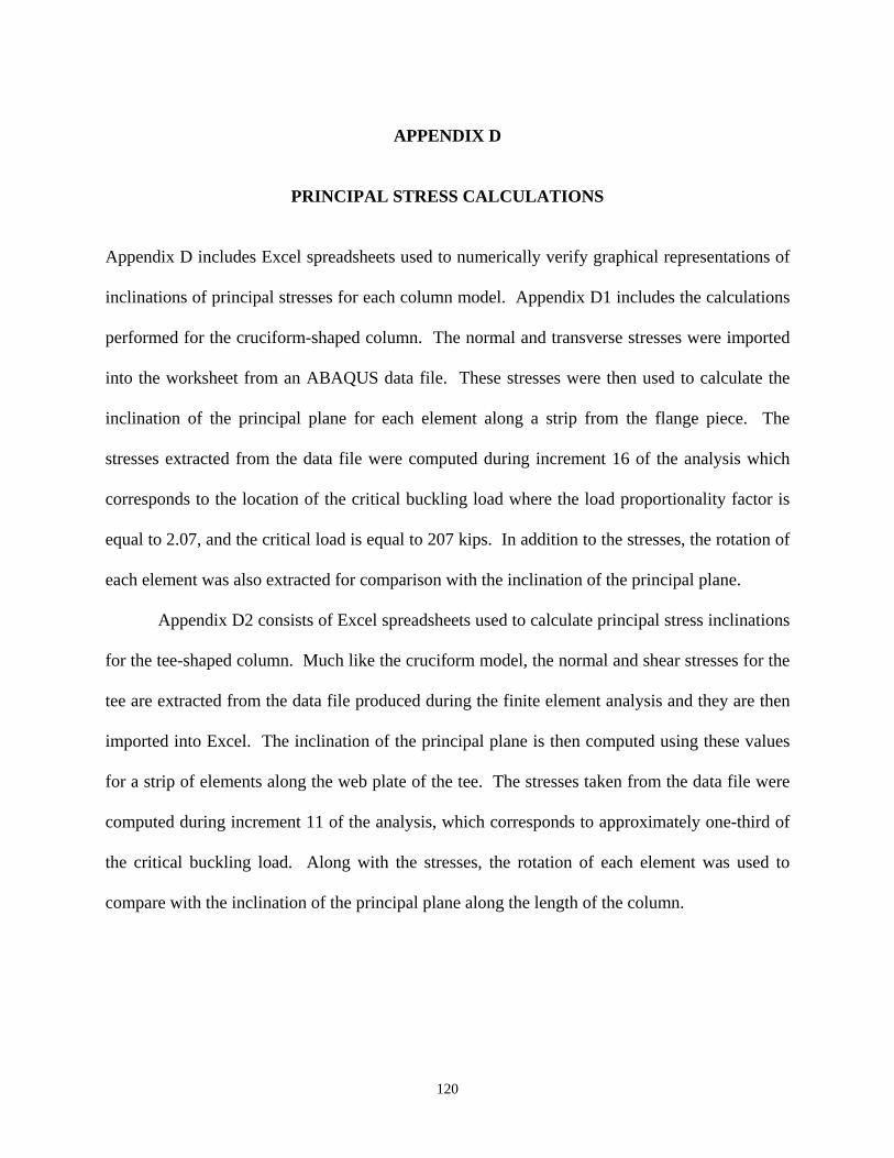
APPENDIX D
PRINCIPAL STRESS CALCULATIONS
Appendix D includes Excel spreadsheets used to numerically verify graphical representations of
inclinations of principal stresses for each column model. Appendix D1 includes the calculations
performed for the cruciform-shaped column. The normal and transverse stresses were imported
into the worksheet from an ABAQUS data file. These stresses were then used to calculate the
inclination of the principal plane for each element along a strip from the flange piece. The
stresses extracted from the data file were computed during increment 16 of the analysis which
corresponds to the location of the critical buckling load where the load proportionality factor is
equal to 2.07, and the critical load is equal to 207 kips. In addition to the stresses, the rotation of
each element was also extracted for comparison with the inclination of the principal plane.
Appendix D2 consists of Excel spreadsheets used to calculate principal stress inclinations
for the tee-shaped column. Much like the cruciform model, the normal and shear stresses for the
tee are extracted from the data file produced during the finite element analysis and they are then
imported into Excel. The inclination of the principal plane is then computed using these values
for a strip of elements along the web plate of the tee. The stresses taken from the data file were
computed during increment 11 of the analysis, which corresponds to approximately one-third of
the critical buckling load. Along with the stresses, the rotation of each element was used to
compare with the inclination of the principal plane along the length of the column.
120

APPENDIX D1
Flange 1 of Cruciform Column (Increment 16)
Table 1: Inclination of Principal Plane (Cruciform) Node UR3 Element S11 S22 S12 θ X X/L 965 0.011343 961 1.691 0.8719 0.1118 -0.1332448 0 0 966 0.011343 962 1.252 -1.681 0.7754 -0.2431879 1 0.0041667 967 0.011617 963 -1.581 -6.525 1.369 -0.252879 2 0.0083333 968 0.011771 964 2.28 -6.378 -0.3057 0.03524987 3 0.0125 969 0.011743 965 -0.1013 -5.942 -0.020382 0.00348959 4 0.0166667 970 0.011833 966 0.7916 -6.85 -0.9435 0.12104727 5 0.0208333 971 0.011828 967 -0.0020969 -6.942 -1.015 0.14228617 6 0.025 972 0.011859 968 0.396 -7.399 -1.265 0.15692012 7 0.0291667 973 0.011863 969 0.02462 -7.695 -1.354 0.16869121 8 0.0333333 974 0.01188 970 0.314 -7.982 -1.476 0.17093139 9 0.0375 975 0.011882 971 0.064465 -8.277 -1.555 0.17843614 10 0.0416667 976 0.011893 972 0.2761 -8.525 -1.652 0.17956399 11 0.0458333 977 0.011891 973 0.085374 -8.795 -1.736 0.18635083 12 0.05 978 0.011896 974 0.2343 -9.028 -1.814 0.18666339 13 0.0541667 979 0.01189 975 0.086475 -9.275 -1.899 0.19270752 14 0.0583333 980 0.011888 976 0.1876 -9.495 -1.96 0.19234018 15 0.0625 981 0.011879 977 0.075715 -9.722 -2.037 0.19703101 16 0.0666667 982 0.011871 978 0.1416 -9.927 -2.085 0.1963262 17 0.0708333 983 0.011857 979 0.059593 -10.13 -2.149 0.19957979 18 0.075 984 0.011844 980 0.1005 -10.33 -2.185 0.19837334 19 0.0791667 985 0.011826 981 0.042234 -10.52 -2.235 0.20017503 20 0.0833333 986 0.011808 982 0.066377 -10.69 -2.263 0.19914273 21 0.0875 987 0.011785 983 0.02592 -10.87 -2.3 0.19973829 22 0.0916667 988 0.011761 984 0.039296 -11.03 -2.32 0.19846432 23 0.0958333 989 0.011734 985 0.01164 -11.2 -2.346 0.19817341 24 0.1 990 0.011705 986 0.018388 -11.35 -2.359 0.19668954 25 0.1041667 991 0.011673 987 -0.0004121 -11.51 -2.377 0.19585145 26 0.1083333 992 0.011638 988 0.0024024 -11.65 -2.385 0.1942736 27 0.1125 993 0.011602 989 -0.010444 -11.8 -2.395 0.19295928 28 0.1166667 994 0.011563 990 -0.0098799 -11.94 -2.399 0.19119013 29 0.1208333 995 0.011521 991 -0.018803 -12.07 -2.404 0.1898067 30 0.125 996 0.011477 992 -0.019472 -12.21 -2.404 0.18783672 31 0.1291667 997 0.01143 993 -0.025836 -12.34 -2.404 0.186121 32 0.1333333 998 0.011381 994 -0.02714 -12.47 -2.401 0.18415672 33 0.1375 999 0.01133 995 -0.031837 -12.6 -2.398 0.18227181 34 0.1416667
1000 0.011276 996 -0.033428 -12.73 -2.392 0.18017155 35 0.1458333 1001 0.01122 997 -0.037028 -12.85 -2.385 0.17819149 36 0.15 1002 0.011162 998 -0.038711 -12.97 -2.377 0.17614924 37 0.1541667 1003 0.011101 999 -0.041573 -13.1 -2.368 0.17396201 38 0.1583333 1004 0.011038 1000 -0.043241 -13.22 -2.358 0.17184891 39 0.1625 1005 0.010972 1001 -0.045593 -13.34 -2.346 0.1696415 40 0.1666667 1006 0.010904 1002 -0.04719 -13.46 -2.334 0.16745736 41 0.1708333 1007 0.010834 1003 -0.049175 -13.58 -2.321 0.16524324 42 0.175 1008 0.010761 1004 -0.050675 -13.7 -2.306 0.16292394 43 0.1791667 1009 0.010687 1005 -0.052389 -13.81 -2.292 0.1608141 44 0.1833333 1010 0.010609 1006 -0.053784 -13.93 -2.276 0.15849101 45 0.1875 1011 0.01053 1007 -0.055289 -14.04 -2.259 0.15624133 46 0.1916667 1012 0.010449 1008 -0.056578 -14.16 -2.242 0.15391524 47 0.1958333 1013 0.010365 1009 -0.057918 -14.27 -2.224 0.15165793 48 0.2 1014 0.010279 1010 -0.059109 -14.39 -2.206 0.14932899 49 0.2041667 1015 0.01019 1011 -0.060315 -14.5 -2.187 0.14706457 50 0.2083333 1016 0.0101 1012 -0.061415 -14.61 -2.167 0.1447638 51 0.2125 1017 0.010007 1013 -0.062511 -14.73 -2.147 0.14239902 52 0.2166667 1018 0.0099128 1014 -0.063529 -14.84 -2.126 0.14009256 53 0.2208333
121

1019 0.0098159 1015 -0.064534 -14.95 -2.104 0.13775156 54 0.225 1020 0.0097169 1016 -0.065479 -15.06 -2.082 0.13543799 55 0.2291667 1021 0.0096159 1017 -0.066405 -15.17 -2.06 0.13315184 56 0.2333333 1022 0.0095127 1018 -0.067285 -15.28 -2.037 0.13083116 57 0.2375 1023 0.0094076 1019 -0.068144 -15.38 -2.014 0.12861801 58 0.2416667 1024 0.0093003 1020 -0.068966 -15.49 -1.99 0.12628864 59 0.2458333 1025 0.0091911 1021 -0.069767 -15.6 -1.965 0.12392585 60 0.25 1026 0.0090799 1022 -0.070537 -15.7 -1.94 0.12166504 61 0.2541667 1027 0.0089667 1023 -0.071286 -15.8 -1.915 0.11942761 62 0.2583333 1028 0.0088515 1024 -0.072009 -15.91 -1.89 0.11714193 63 0.2625 1029 0.0087345 1025 -0.072712 -16.01 -1.864 0.11489262 64 0.2666667 1030 0.0086155 1026 -0.073392 -16.11 -1.837 0.11260711 65 0.2708333 1031 0.0084946 1027 -0.074054 -16.21 -1.81 0.1103449 66 0.275 1032 0.0083719 1028 -0.074694 -16.31 -1.783 0.10810572 67 0.2791667 1033 0.0082474 1029 -0.075318 -16.41 -1.755 0.10583083 68 0.2833333 1034 0.0081211 1030 -0.075922 -16.5 -1.727 0.10364023 69 0.2875 1035 0.0079929 1031 -0.07651 -16.6 -1.699 0.10140953 70 0.2916667 1036 0.0078631 1032 -0.077081 -16.69 -1.67 0.09920169 71 0.2958333 1037 0.0077315 1033 -0.077635 -16.79 -1.641 0.09695693 72 0.3 1038 0.0075982 1034 -0.078174 -16.88 -1.612 0.09478979 73 0.3041667 1039 0.0074632 1035 -0.078697 -16.97 -1.582 0.09258477 74 0.3083333 1040 0.0073265 1036 -0.079205 -17.06 -1.552 0.09039932 75 0.3125 1041 0.0071883 1037 -0.079699 -17.15 -1.522 0.08823327 76 0.3166667 1042 0.0070485 1038 -0.080178 -17.23 -1.491 0.08607906 77 0.3208333 1043 0.0069071 1039 -0.080643 -17.32 -1.46 0.08389369 78 0.325 1044 0.0067641 1040 -0.081094 -17.4 -1.429 0.081774 79 0.3291667 1045 0.0066197 1041 -0.081532 -17.48 -1.398 0.07967071 80 0.3333333 1046 0.0064738 1042 -0.081956 -17.56 -1.366 0.07752785 81 0.3375 1047 0.0063264 1043 -0.082368 -17.64 -1.334 0.07540152 82 0.3416667 1048 0.0061777 1044 -0.082766 -17.72 -1.301 0.07323613 83 0.3458333 1049 0.0060276 1045 -0.083151 -17.8 -1.269 0.07114271 84 0.35 1050 0.0058761 1046 -0.083524 -17.87 -1.236 0.06904869 85 0.3541667 1051 0.0057233 1047 -0.083885 -17.94 -1.203 0.06696853 86 0.3583333 1052 0.0055692 1048 -0.084233 -18.01 -1.169 0.06484733 87 0.3625 1053 0.0054139 1049 -0.084569 -18.08 -1.136 0.06279489 88 0.3666667 1054 0.0052574 1050 -0.084893 -18.15 -1.102 0.06070159 89 0.3708333 1055 0.0050996 1051 -0.085206 -18.21 -1.068 0.05865427 90 0.375 1056 0.0049408 1052 -0.085507 -18.28 -1.034 0.05658754 91 0.3791667 1057 0.0047808 1053 -0.085796 -18.34 -0.9993 0.05452637 92 0.3833333 1058 0.0046198 1054 -0.086074 -18.4 -0.9647 0.05248217 93 0.3875 1059 0.0044577 1055 -0.08634 -18.45 -0.9298 0.05046059 94 0.3916667 1060 0.0042946 1056 -0.086596 -18.51 -0.8948 0.04841676 95 0.3958333 1061 0.0041305 1057 -0.08684 -18.56 -0.8597 0.0464041 96 0.4 1062 0.0039655 1058 -0.087073 -18.61 -0.8243 0.04438465 97 0.4041667 1063 0.0037996 1059 -0.087296 -18.66 -0.7888 0.04236923 98 0.4083333 1064 0.0036329 1060 -0.087508 -18.71 -0.7531 0.04035251 99 0.4125 1065 0.0034653 1061 -0.087709 -18.75 -0.7173 0.03836035 100 0.4166667 1066 0.0032969 1062 -0.087899 -18.8 -0.6814 0.03635076 101 0.4208333 1067 0.0031278 1063 -0.088079 -18.84 -0.6453 0.03435829 102 0.425 1068 0.002958 1064 -0.088248 -18.88 -0.6091 0.03236787 103 0.4291667 1069 0.0027875 1065 -0.088408 -18.91 -0.5728 0.03039563 104 0.4333333 1070 0.0026163 1066 -0.088556 -18.95 -0.5363 0.02840307 105 0.4375 1071 0.0024446 1067 -0.088695 -18.98 -0.4998 0.02643197 106 0.4416667 1072 0.0022723 1068 -0.088823 -19.01 -0.4632 0.02446097 107 0.4458333 1073 0.0020995 1069 -0.088942 -19.04 -0.4264 0.02248489 108 0.45 1074 0.0019263 1070 -0.08905 -19.06 -0.3896 0.02052513 109 0.4541667 1075 0.0017526 1071 -0.089148 -19.09 -0.3528 0.01855906 110 0.4583333 1076 0.0015784 1072 -0.089237 -19.11 -0.3158 0.01659681 111 0.4625 1077 0.001404 1073 -0.089315 -19.12 -0.2788 0.01464583 112 0.4666667 1078 0.0012292 1074 -0.089384 -19.14 -0.2417 0.01268453 113 0.4708333 1079 0.0010541 1075 -0.089442 -19.15 -0.2046 0.01073256 114 0.475 1080 0.0008788 1076 -0.089491 -19.17 -0.1675 0.00877769 115 0.4791667 1081 0.0007033 1077 -0.08953 -19.18 -0.1303 0.00682497 116 0.4833333 1082 0.0005276 1078 -0.08956 -19.18 -0.093083 0.00487574 117 0.4875 1083 0.0003518 1079 -0.089579 -19.19 -0.055857 0.00292435 118 0.4916667
122

1084 0.0001759 1080 -0.089589 -19.19 -0.01862 0.00097485 119 0.4958333 1085 5.242E-14 1081 -0.089589 -19.19 0.01862 -0.0009748 120 0.5 1086 -0.0001759 1082 -0.089579 -19.19 0.055857 -0.0029244 121 0.5041667 1087 -0.0003518 1083 -0.08956 -19.18 0.093083 -0.0048757 122 0.5083333 1088 -0.0005276 1084 -0.08953 -19.18 0.1303 -0.006825 123 0.5125 1089 -0.0007033 1085 -0.089491 -19.17 0.1675 -0.0087777 124 0.5166667 1090 -0.0008788 1086 -0.089442 -19.15 0.2046 -0.0107326 125 0.5208333 1091 -0.0010541 1087 -0.089384 -19.14 0.2417 -0.0126845 126 0.525 1092 -0.0012292 1088 -0.089315 -19.12 0.2788 -0.0146458 127 0.5291667 1093 -0.001404 1089 -0.089237 -19.11 0.3158 -0.0165968 128 0.5333333 1094 -0.0015784 1090 -0.089148 -19.09 0.3528 -0.0185591 129 0.5375 1095 -0.0017526 1091 -0.08905 -19.06 0.3896 -0.0205251 130 0.5416667 1096 -0.0019263 1092 -0.088942 -19.04 0.4264 -0.0224849 131 0.5458333 1097 -0.0020995 1093 -0.088823 -19.01 0.4632 -0.024461 132 0.55 1098 -0.0022723 1094 -0.088695 -18.98 0.4998 -0.026432 133 0.5541667 1099 -0.0024446 1095 -0.088556 -18.95 0.5363 -0.0284031 134 0.5583333 1100 -0.0026163 1096 -0.088408 -18.91 0.5728 -0.0303956 135 0.5625 1101 -0.0027875 1097 -0.088248 -18.88 0.6091 -0.0323679 136 0.5666667 1102 -0.002958 1098 -0.088079 -18.84 0.6453 -0.0343583 137 0.5708333 1103 -0.0031278 1099 -0.087899 -18.8 0.6814 -0.0363508 138 0.575 1104 -0.0032969 1100 -0.087709 -18.75 0.7173 -0.0383604 139 0.5791667 1105 -0.0034653 1101 -0.087508 -18.71 0.7531 -0.0403525 140 0.5833333 1106 -0.0036329 1102 -0.087296 -18.66 0.7888 -0.0423692 141 0.5875 1107 -0.0037996 1103 -0.087073 -18.61 0.8243 -0.0443847 142 0.5916667 1108 -0.0039655 1104 -0.08684 -18.56 0.8597 -0.0464041 143 0.5958333 1109 -0.0041305 1105 -0.086596 -18.51 0.8948 -0.0484168 144 0.6 1110 -0.0042946 1106 -0.08634 -18.45 0.9298 -0.0504606 145 0.6041667 1111 -0.0044577 1107 -0.086074 -18.4 0.9647 -0.0524822 146 0.6083333 1112 -0.0046198 1108 -0.085796 -18.34 0.9993 -0.0545264 147 0.6125 1113 -0.0047808 1109 -0.085507 -18.28 1.034 -0.0565875 148 0.6166667 1114 -0.0049408 1110 -0.085206 -18.21 1.068 -0.0586543 149 0.6208333 1115 -0.0050996 1111 -0.084893 -18.15 1.102 -0.0607016 150 0.625 1116 -0.0052574 1112 -0.084569 -18.08 1.136 -0.0627949 151 0.6291667 1117 -0.0054139 1113 -0.084233 -18.01 1.169 -0.0648473 152 0.6333333 1118 -0.0055692 1114 -0.083885 -17.94 1.203 -0.0669685 153 0.6375 1119 -0.0057233 1115 -0.083524 -17.87 1.236 -0.0690487 154 0.6416667 1120 -0.0058761 1116 -0.083151 -17.8 1.269 -0.0711427 155 0.6458333 1121 -0.0060276 1117 -0.082766 -17.72 1.301 -0.0732361 156 0.65 1122 -0.0061777 1118 -0.082368 -17.64 1.334 -0.0754015 157 0.6541667 1123 -0.0063264 1119 -0.081956 -17.56 1.366 -0.0775278 158 0.6583333 1124 -0.0064738 1120 -0.081532 -17.48 1.398 -0.0796707 159 0.6625 1125 -0.0066197 1121 -0.081094 -17.4 1.429 -0.081774 160 0.6666667 1126 -0.0067641 1122 -0.080643 -17.32 1.46 -0.0838937 161 0.6708333 1127 -0.0069071 1123 -0.080178 -17.23 1.491 -0.0860791 162 0.675 1128 -0.0070485 1124 -0.079699 -17.15 1.522 -0.0882333 163 0.6791667 1129 -0.0071883 1125 -0.079205 -17.06 1.552 -0.0903993 164 0.6833333 1130 -0.0073265 1126 -0.078697 -16.97 1.582 -0.0925848 165 0.6875 1131 -0.0074632 1127 -0.078174 -16.88 1.612 -0.0947898 166 0.6916667 1132 -0.0075982 1128 -0.077635 -16.79 1.641 -0.0969569 167 0.6958333 1133 -0.0077315 1129 -0.077081 -16.69 1.67 -0.0992017 168 0.7 1134 -0.0078631 1130 -0.07651 -16.6 1.699 -0.1014095 169 0.7041667 1135 -0.0079929 1131 -0.075922 -16.5 1.727 -0.1036402 170 0.7083333 1136 -0.0081211 1132 -0.075318 -16.41 1.755 -0.1058308 171 0.7125 1137 -0.0082474 1133 -0.074694 -16.31 1.783 -0.1081057 172 0.7166667 1138 -0.0083719 1134 -0.074054 -16.21 1.81 -0.1103449 173 0.7208333 1139 -0.0084946 1135 -0.073392 -16.11 1.837 -0.1126071 174 0.725 1140 -0.0086155 1136 -0.072712 -16.01 1.864 -0.1148926 175 0.7291667 1141 -0.0087345 1137 -0.072009 -15.91 1.89 -0.1171419 176 0.7333333 1142 -0.0088515 1138 -0.071286 -15.8 1.915 -0.1194276 177 0.7375 1143 -0.0089667 1139 -0.070537 -15.7 1.94 -0.121665 178 0.7416667 1144 -0.0090799 1140 -0.069767 -15.6 1.965 -0.1239258 179 0.7458333 1145 -0.0091911 1141 -0.068966 -15.49 1.99 -0.1262886 180 0.75 1146 -0.0093003 1142 -0.068144 -15.38 2.014 -0.128618 181 0.7541667 1147 -0.0094076 1143 -0.067285 -15.28 2.037 -0.1308312 182 0.7583333 1148 -0.0095127 1144 -0.066405 -15.17 2.06 -0.1331518 183 0.7625
123

1149 -0.0096159 1145 -0.065479 -15.06 2.082 -0.135438 184 0.7666667 1150 -0.0097169 1146 -0.064534 -14.95 2.104 -0.1377516 185 0.7708333 1151 -0.0098159 1147 -0.063529 -14.84 2.126 -0.1400926 186 0.775 1152 -0.0099128 1148 -0.062511 -14.73 2.147 -0.142399 187 0.7791667 1153 -0.010007 1149 -0.061415 -14.61 2.167 -0.1447638 188 0.7833333 1154 -0.0101 1150 -0.060315 -14.5 2.187 -0.1470646 189 0.7875 1155 -0.01019 1151 -0.059109 -14.39 2.206 -0.149329 190 0.7916667 1156 -0.010279 1152 -0.057918 -14.27 2.224 -0.1516579 191 0.7958333 1157 -0.010365 1153 -0.056578 -14.16 2.242 -0.1539152 192 0.8 1158 -0.010449 1154 -0.055289 -14.04 2.259 -0.1562413 193 0.8041667 1159 -0.01053 1155 -0.053784 -13.93 2.276 -0.158491 194 0.8083333 1160 -0.010609 1156 -0.052389 -13.81 2.292 -0.1608141 195 0.8125 1161 -0.010687 1157 -0.050675 -13.7 2.306 -0.1629239 196 0.8166667 1162 -0.010761 1158 -0.049175 -13.58 2.321 -0.1652432 197 0.8208333 1163 -0.010834 1159 -0.04719 -13.46 2.334 -0.1674574 198 0.825 1164 -0.010904 1160 -0.045593 -13.34 2.346 -0.1696415 199 0.8291667 1165 -0.010972 1161 -0.043241 -13.22 2.358 -0.1718489 200 0.8333333 1166 -0.011038 1162 -0.041573 -13.1 2.368 -0.173962 201 0.8375 1167 -0.011101 1163 -0.038711 -12.97 2.377 -0.1761492 202 0.8416667 1168 -0.011162 1164 -0.037028 -12.85 2.385 -0.1781915 203 0.8458333 1169 -0.01122 1165 -0.033428 -12.73 2.392 -0.1801716 204 0.85 1170 -0.011276 1166 -0.031837 -12.6 2.398 -0.1822718 205 0.8541667 1171 -0.01133 1167 -0.02714 -12.47 2.401 -0.1841567 206 0.8583333 1172 -0.011381 1168 -0.025836 -12.34 2.404 -0.186121 207 0.8625 1173 -0.01143 1169 -0.019472 -12.21 2.404 -0.1878367 208 0.8666667 1174 -0.011477 1170 -0.018803 -12.07 2.404 -0.1898067 209 0.8708333 1175 -0.011521 1171 -0.0098799 -11.94 2.399 -0.1911901 210 0.875 1176 -0.011563 1172 -0.010444 -11.8 2.395 -0.1929593 211 0.8791667 1177 -0.011602 1173 0.0024024 -11.65 2.385 -0.1942736 212 0.8833333 1178 -0.011638 1174 -0.0004121 -11.51 2.377 -0.1958514 213 0.8875 1179 -0.011673 1175 0.018388 -11.35 2.359 -0.1966895 214 0.8916667 1180 -0.011705 1176 0.01164 -11.2 2.346 -0.1981734 215 0.8958333 1181 -0.011734 1177 0.039296 -11.03 2.32 -0.1984643 216 0.9 1182 -0.011761 1178 0.02592 -10.87 2.3 -0.1997383 217 0.9041667 1183 -0.011785 1179 0.066377 -10.69 2.263 -0.1991427 218 0.9083333 1184 -0.011808 1180 0.042234 -10.52 2.235 -0.200175 219 0.9125 1185 -0.011826 1181 0.1005 -10.33 2.185 -0.1983733 220 0.9166667 1186 -0.011844 1182 0.059593 -10.13 2.149 -0.1995798 221 0.9208333 1187 -0.011857 1183 0.1416 -9.927 2.085 -0.1963262 222 0.925 1188 -0.011871 1184 0.075715 -9.722 2.037 -0.197031 223 0.9291667 1189 -0.011879 1185 0.1876 -9.495 1.96 -0.1923402 224 0.9333333 1190 -0.011888 1186 0.086475 -9.275 1.899 -0.1927075 225 0.9375 1191 -0.01189 1187 0.2343 -9.028 1.814 -0.1866634 226 0.9416667 1192 -0.011896 1188 0.085374 -8.795 1.736 -0.1863508 227 0.9458333 1193 -0.011891 1189 0.2761 -8.525 1.652 -0.179564 228 0.95 1194 -0.011893 1190 0.064465 -8.277 1.555 -0.1784361 229 0.9541667 1195 -0.011882 1191 0.314 -7.982 1.476 -0.1709314 230 0.9583333 1196 -0.01188 1192 0.02462 -7.695 1.354 -0.1686912 231 0.9625 1197 -0.011863 1193 0.396 -7.399 1.265 -0.1569201 232 0.9666667 1198 -0.011859 1194 -0.0020969 -6.942 1.015 -0.1422862 233 0.9708333 1199 -0.011828 1195 0.7916 -6.85 0.9435 -0.1210473 234 0.975 1200 -0.011833 1196 -0.1013 -5.942 0.020382 -0.0034896 235 0.9791667 1201 -0.011743 1197 2.28 -6.378 0.3057 -0.0352499 236 0.9833333 1202 -0.011771 1198 -1.581 -6.525 -1.369 0.25287899 237 0.9875 1203 -0.011617 1199 1.252 -1.681 -0.7754 0.24318794 238 0.9916667 1204 -0.011343 1200 1.691 0.8719 -0.1118 0.13324482 239 0.9958333 1205 -0.011343 240 1
124

APPENDIX D2
Flange Plate of Tee Column (Increment 11)
Table 2: Inclination of Principal Plane (Tee) Node UR3 Element S11 S22 S12 X/L θ559 -0.000597 461 -0.08194 -1.215 -0.21800 0.000 -0.184560 -0.000612 462 0.06172 -1.493 -0.15520 0.011 -0.099561 -0.000595 463 -0.00896 -1.711 -0.26130 0.022 -0.149562 -0.000595 464 -0.00306 -1.668 -0.27190 0.033 -0.158563 -0.000592 465 -0.00083 -1.592 -0.25730 0.044 -0.156564 -0.000590 466 0.01092 -1.556 -0.26120 0.055 -0.161565 -0.000587 467 0.00351 -1.524 -0.27050 0.066 -0.170566 -0.000583 468 0.00734 -1.499 -0.27540 0.077 -0.175567 -0.000578 469 0.00265 -1.472 -0.28340 0.088 -0.183568 -0.000573 470 0.00283 -1.442 -0.28540 0.099 -0.188569 -0.000568 471 0.00101 -1.411 -0.28780 0.110 -0.194570 -0.000561 472 0.00075 -1.378 -0.28730 0.121 -0.197571 -0.000554 473 -0.00026 -1.345 -0.28660 0.132 -0.201572 -0.000546 474 -0.00024 -1.312 -0.28460 0.143 -0.205573 -0.000538 475 -0.00118 -1.278 -0.28230 0.154 -0.208574 -0.000529 476 -0.00087 -1.245 -0.27940 0.165 -0.211575 -0.000520 477 -0.00184 -1.213 -0.27600 0.176 -0.214576 -0.000510 478 -0.00142 -1.181 -0.27230 0.187 -0.216577 -0.000499 479 -0.00235 -1.149 -0.26810 0.198 -0.219578 -0.000488 480 -0.00194 -1.118 -0.26370 0.209 -0.221579 -0.000476 481 -0.00279 -1.088 -0.25900 0.220 -0.223580 -0.000464 482 -0.00246 -1.058 -0.25390 0.231 -0.224581 -0.000451 483 -0.00320 -1.029 -0.24850 0.242 -0.226582 -0.000437 484 -0.00298 -1.001 -0.24280 0.253 -0.226583 -0.000423 485 -0.00360 -0.974 -0.23690 0.264 -0.227584 -0.000409 486 -0.00349 -0.947 -0.23060 0.275 -0.227585 -0.000394 487 -0.00401 -0.921 -0.22410 0.286 -0.227586 -0.000378 488 -0.00399 -0.896 -0.21720 0.297 -0.227587 -0.000362 489 -0.00443 -0.872 -0.21010 0.308 -0.226588 -0.000346 490 -0.00447 -0.849 -0.20260 0.319 -0.224589 -0.000329 491 -0.00485 -0.827 -0.19490 0.330 -0.221590 -0.000312 492 -0.00494 -0.805 -0.18690 0.341 -0.218591 -0.000294 493 -0.00526 -0.785 -0.17860 0.352 -0.215592 -0.000276 494 -0.00539 -0.766 -0.17000 0.363 -0.210593 -0.000258 495 -0.00567 -0.748 -0.16120 0.374 -0.205594 -0.000239 496 -0.00582 -0.731 -0.15210 0.385 -0.199595 -0.000220 497 -0.00607 -0.715 -0.14270 0.396 -0.191596 -0.000201 498 -0.00622 -0.700 -0.13310 0.407 -0.183597 -0.000181 499 -0.00645 -0.686 -0.12320 0.418 -0.174598 -0.000161 500 -0.00661 -0.674 -0.11310 0.429 -0.163599 -0.000141 501 -0.00681 -0.663 -0.10270 0.440 -0.152600 -0.000121 502 -0.00696 -0.653 -0.09206 0.451 -0.139601 -0.000100 503 -0.00714 -0.644 -0.08122 0.462 -0.125602 -0.000079 504 -0.00729 -0.636 -0.07016 0.473 -0.110603 -0.000059 505 -0.00745 -0.630 -0.05889 0.484 -0.093604 -0.000038 506 -0.00758 -0.625 -0.04742 0.495 -0.076605 -0.000016 507 -0.00772 -0.622 -0.03576 0.505 -0.058606 0.000005 508 -0.00784 -0.620 -0.02391 0.516 -0.039607 0.000026 509 -0.00794 -0.619 -0.01190 0.527 -0.019608 0.000047 510 -0.00806 -0.619 0.00028 0.538 0.000609 0.000068 511 -0.00813 -0.621 0.01260 0.549 0.021610 0.000090 512 -0.00823 -0.625 0.02506 0.560 0.041611 0.000111 513 -0.00827 -0.629 0.03764 0.571 0.060612 0.000132 514 -0.00835 -0.635 0.05033 0.582 0.080613 0.000153 515 -0.00836 -0.643 0.06311 0.593 0.098
125

614 0.000174 516 -0.00843 -0.652 0.07597 0.604 0.116615 0.000195 517 -0.00840 -0.662 0.08890 0.615 0.133616 0.000215 518 -0.00846 -0.674 0.10190 0.626 0.149617 0.000235 519 -0.00837 -0.687 0.11490 0.637 0.163618 0.000256 520 -0.00843 -0.702 0.12790 0.648 0.177619 0.000275 521 -0.00829 -0.718 0.14090 0.659 0.189620 0.000295 522 -0.00836 -0.736 0.15390 0.670 0.200621 0.000314 523 -0.00813 -0.755 0.16690 0.681 0.210622 0.000333 524 -0.00822 -0.775 0.17980 0.692 0.219623 0.000351 525 -0.00791 -0.797 0.19270 0.703 0.227624 0.000370 526 -0.00804 -0.820 0.20540 0.714 0.234625 0.000387 527 -0.00761 -0.844 0.21800 0.725 0.240626 0.000405 528 -0.00780 -0.870 0.23050 0.736 0.245627 0.000421 529 -0.00724 -0.897 0.24280 0.747 0.250628 0.000438 530 -0.00750 -0.926 0.25500 0.758 0.253629 0.000453 531 -0.00679 -0.956 0.26690 0.769 0.256630 0.000468 532 -0.00711 -0.987 0.27860 0.780 0.259631 0.000483 533 -0.00625 -1.019 0.29000 0.791 0.260632 0.000497 534 -0.00659 -1.052 0.30100 0.802 0.261633 0.000511 535 -0.00557 -1.086 0.31170 0.813 0.262634 0.000523 536 -0.00583 -1.122 0.32180 0.824 0.262635 0.000536 537 -0.00470 -1.158 0.33130 0.835 0.261636 0.000547 538 -0.00470 -1.195 0.34010 0.846 0.260637 0.000558 539 -0.00347 -1.233 0.34790 0.857 0.257638 0.000568 540 -0.00298 -1.270 0.35480 0.868 0.255639 0.000577 541 -0.00152 -1.308 0.35970 0.879 0.252640 0.000585 542 -0.00045 -1.345 0.36340 0.890 0.248641 0.000593 543 0.00195 -1.381 0.36330 0.901 0.242642 0.000600 544 0.00295 -1.415 0.36220 0.912 0.236643 0.000607 545 0.00819 -1.447 0.35390 0.923 0.226644 0.000612 546 0.00590 -1.475 0.34700 0.934 0.219645 0.000617 547 0.01339 -1.511 0.33460 0.945 0.207646 0.000621 548 0.00348 -1.551 0.32600 0.956 0.199647 0.000623 549 -0.00006 -1.631 0.33550 0.967 0.195648 0.000626 550 -0.00287 -1.674 0.31750 0.978 0.182649 0.000627 551 0.06473 -1.446 0.20220 0.989 0.131650 0.000644 552 -0.06446 -1.115 0.23800 1.000 0.213651 0.000628 1.011
126

BIBLIOGRAPHY
1. ABAQUS, (2003) ABAQUS Standard User’s Manual, Version 6.4, Volumes 1 to 3, Hibbit, Karlsson & Sorensen, Inc., Pawtucket, Rhode Island, USA.
2. ABAQUS, (2003) ABAQUS Theory Manual, Version 6.4, Hibbit, Karlsson & Sorensen, Inc., Pawtucket, Rhode Island, USA.
3. Bleich, F., (1952) Buckling Strength of Metal Structures, McGraw-Hill, New York, USA.
4. Chen, S.F., (1980) “Lateral-Torsional Buckling of T-Section Steel Beam-Columns”, Structural Stability Research Council Meeting translated from Journal of Xian Institute of Metallurgy and Construction Engineering, No. 3, 1978, Xian, Shaanxi, China.
5. Earls, C.J., Shah, B.J., (2002) “High Performance Steel Bridge Girder Compactness”, Journal of Constructional Steel Research, Elsevier Science Ltd., Great Britain, Vol. 58, pp. 859-880.
6. Galambos, T.V., (1998) Guide to Stability Design Criteria for Metal Structures, Fifth Edition, John Wiley & Sons, Inc., New York, New York, USA.
7. Galambos, T.V., (1968) Structural Members and Frames, Prentice-Hall, Englewood Cliffs, New Jersey, USA.
8. Goodier, J.N., (1950) “Elastic Torsion in the Presence of Initial Axial Stress”, American Society of Mechanical Engineers Journal of Applied Mechanics, USA.
9. Michell, A.G.M., (1899) “Elastic Stability of Long Beams Under Transverse Forces”, Phil. Mag., Vol. 48.
10. Ojalvo, M., (1982) “Discussion of “Lateral-Torsional Buckling of Tapered I-beams”, Journal of the Structural Division, ASCE, Vol. 108, No.2, USA.
11. Ojalvo, M., (1987) “Discussion of “Buckling of Mono-symmetric I-beams Under Moment Gradient”, Journal of the Engineering Mechanics Division, ASCE, Vol. 109, No.3, USA.
12. Ojalvo, M., (1990) Thin-Walled Bars with Open Profiles, The Olive Press, Columbus, Ohio, USA.
13. Prandtl, L., (1899) “Kipperscheinungen”, Thesis, Munich.
14. Timoshenko, S.P., (1905) Lateral Buckling of Beams, Bulletin Polytechnical Institute, Vol. 4(5), Saint Petersburg.
127

15. Vlasov, V.Z., (1961) Thin-Walled Elastic Beams, 2d ed. rev. and augm. Translated from Russian [by Y. Schectman], Jerusalem, Published for the National Science Foundation, Washington, D.C., by the Israel Program for Scientific Translations.
16. Wagner, H., (1929) “Verdrehung Und Knickung Von Offenen Profilen”, 25th Anniversary Publication, Technische Hochscule, Danzig, Translated in NACA Tech. Mem. 807, 1936.
128