Embed Size (px)
Citation preview

On the Use of Conformal Maps for the Acceleration ofConvergence of the Trapezoidal Rule and Sinc
Numerical Methods
Richard Mikael Slevinsky† andSheehan Olver‡
†Mathematical Institute, University of Oxford
‡School of Mathematics and Statistics, TheUniversity of Sydney
Numerical Analysis Seminar, The Universityof Tokyo
August 6, 2015
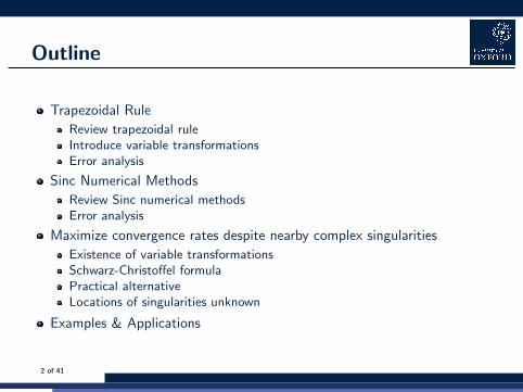
Outline
Trapezoidal Rule
Review trapezoidal ruleIntroduce variable transformationsError analysis
Sinc Numerical Methods
Review Sinc numerical methodsError analysis
Maximize convergence rates despite nearby complex singularities
Existence of variable transformationsSchwarz-Christoffel formulaPractical alternativeLocations of singularities unknown
Examples & Applications
2 of 41

Trapezoidal Rule
The trapezoidal rule
∫ b
a
f (x)dx ≈ (b − a)
[f (a) + f (b)
2
].
The composite version T (h) = hn−1∑k=1
f (xk−1) + f (xk)
2, where h =
b − a
n
and xk = a + k h.
Euler-Maclaurin summation formula T (h)−∫ b
a
f (x)dx ∼∞∑l=1
h2l B2l
(2l)!
(f (2l−1)(b)− f (2l−1)(a)
), as h→ 0.
If f (n)(·)→ 0 at endpoints, the convergence is faster than any power of h[Trefethen and Weidemann 2015].
Variable transformations φ : R→ (a, b) with exponential decay [Stenger1970] and [Takahasi and Mori 1974].
3 of 41

Preview of Optimization
Consider the integral for ε > 0:
∫ 1
−1
ε2
x2 + ε2dx = ε tan−1(ε−1).
Variable transformations which induce endpoint decay are:
x = φSE (t) = tanh(t/2), x = φDE (t) = tanh(π/2 sinh(t)).
φ′SE (t) = sech2(t/2)/2, φ′DE (t) = sech2(π/2 sinh(t))π/2 cosh(t).
��
����
�
���
�
����
�� ���� � ��� �
�
����
����
�
���
���
����
�� �� � � �
�
����
��
����
�
���
�
���
����
�� �� � � �
�
Integrand ε = 1 SE transformation DE transformation
4 of 41
Preview of Optimization
��
��
����
���
���
���
���
�
����������������������
� �� ��� ��� ��� ���
�������
��
��
����
���
���
���
���
�
����������������������
� �� ��� ��� ��� ���
�������
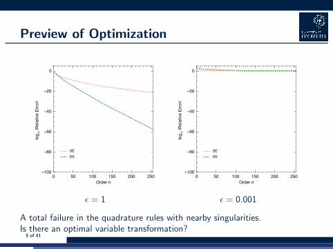
ε = 1 ε = 0.001
A total failure in the quadrature rules with nearby singularities.Is there an optimal variable transformation?
5 of 41

Preview of Optimization
��
��
������������
����
���
���
���
���
�
����������������������
� �� ��� ��� ��� ���
�������
��
��
������������
����
���
���
���
���
�
����������������������
� �� ��� ��� ��� ���
�������
ε = 1 ε = 0.001
x = φDEopt(t) = tanh(tan−1(ε) sinh(t)),
φ′DEopt(t) = sech2(tan−1(ε) sinh(t)) tan−1(ε) cosh(t).6 of 41
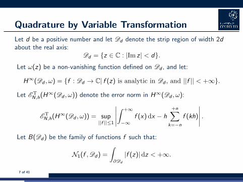
Quadrature by Variable Transformation
Let d be a positive number and let Dd denote the strip region of width 2dabout the real axis:
Dd = {z ∈ C : |Im z | < d}.
Let ω(z) be a non-vanishing function defined on Dd , and let:
H∞(Dd , ω) = {f : Dd → C| f (z) is analytic in Dd , and ||f || < +∞}.
Let E TN,h(H∞(Dd , ω)) denote the error norm in H∞(Dd , ω):
E TN,h(H∞(Dd , ω)) = sup
||f ||≤1
∣∣∣∣∣∫ +∞
−∞f (x)dx − h
+n∑k=−n
f (kh)
∣∣∣∣∣ .Let B(Dd) be the family of functions f such that:
N1(f ,Dd) =
∫∂Dd
|f (z)|dz < +∞.
7 of 41

Quadrature by Variable Transformation
Theorem [Sugihara 1997] Suppose:
1 ω(z) ∈ B(Dd);
2 ω(z) does not vanish at any point in Dd and takes real values on the realaxis;
3 α1 exp (−(β|x |ρ)) ≤ |ω(x)| ≤ α2 exp (−(β|x |ρ)) , x ∈ R,where α1, α2, β > 0 and ρ ≥ 1.
Then:E TN,h(H∞(Dd , ω)) ≤ Cd,ω exp
(−(πdβN)
ρρ+1
),
where N = 2n + 1, the mesh size h is chosen optimally as:
h = (2πd)1
ρ+1 (βn)−ρ
ρ+1 ,
and Cd,ω is a constant depending on d and ω.
8 of 41
Quadrature by Variable Transformation
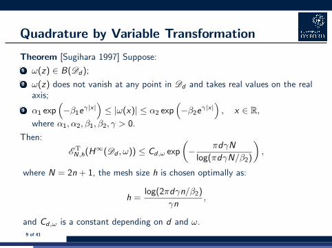
Theorem [Sugihara 1997] Suppose:
1 ω(z) ∈ B(Dd);
2 ω(z) does not vanish at any point in Dd and takes real values on the realaxis;
3 α1 exp(−β1e
γ|x|)≤ |ω(x)| ≤ α2 exp
(−β2e
γ|x|), x ∈ R,
where α1, α2, β1, β2, γ > 0.
Then:
E TN,h(H∞(Dd , ω)) ≤ Cd,ω exp
(− πdγN
log(πdγN/β2)
),
where N = 2n + 1, the mesh size h is chosen optimally as:
h =log(2πdγn/β2)
γn,
and Cd,ω is a constant depending on d and ω.9 of 41

Sinc Numerical Methods
Let us consider the N(= 2n + 1)-point Sinc approximation of a function onthe real line:
f (x) ≈+n∑
j=−n
f (j h)S(j , h)(x),
where S(j , h)(x) is the so-called Sinc function:
S(j , h)(x) =sin[π(x/h − j)]
π(x/h − j),
and where the step size h is suitably chosen for a given positive integer n.Let E Sinc
N,h (H∞(Dd , ω)) denote the error norm in H∞(Dd , ω):
E SincN,h (H∞(Dd , ω)) = sup
||f ||≤1
supx∈R
∣∣∣∣∣∣f (x)−+n∑
j=−n
f (j h)S(j , h)(x)
∣∣∣∣∣∣ .
10 of 41

Sinc Numerical Methods
Theorem [Sugihara 2003] Suppose:
1 ω(z) ∈ B(Dd);
2 ω(z) does not vanish at any point in Dd and takes real values on the realaxis;
3 α1 exp (−(β|x |ρ)) ≤ |ω(x)| ≤ α2 exp (−(β|x |ρ)) , x ∈ R,where α1, α2, β > 0 and ρ ≥ 1.
Then:
E SincN,h (H∞(Dd , ω)) ≤ Cd,ωN
1ρ+1 exp
(−(πdβN
2
) ρρ+1
),
where N = 2n + 1, the mesh size h is chosen optimally as:
h = (πd)1
ρ+1 (βn)−ρ
ρ+1 ,
and Cd,ω is a constant depending on d and ω.11 of 41

Sinc Numerical Methods
Theorem [Sugihara 2003] Suppose:
1 ω(z) ∈ B(Dd);
2 ω(z) does not vanish at any point in Dd and takes real values on the realaxis;
3 α1 exp(−β1e
γ|x|)≤ |ω(x)| ≤ α2 exp
(−β2e
γ|x|), x ∈ R,
where α1, α2, β1, β2, γ > 0.
Then:
E SincN,h (H∞(Dd , ω)) ≤ Cd,ω exp
(− πdγN
2 log(πdγN/(2β2))
),
where N = 2n + 1, the mesh size h is chosen optimally as:
h =log(πdγn/β2)
γn,
and Cd,ω is a constant depending on d and ω.12 of 41

An Upper Bound
Nonexistence Theorem [Sugihara 1997] There exists no function ω(z) thatsatisfies at once:
1 ω(z) ∈ B(Dd);
2 ω(z) does not vanish at any point in Dd and takes real values on the realaxis;
3 ω(x) = O(exp(−βeγ|x|)
)as |x | → ∞, where β > 0, and dγ > π/2.
Conclusion:
Based essentially on the celebrated Pragmen-Lindelof principle, Sugiharaexcludes utility of further decay.
Optimality of the DE transformation for the trapezoidal rule and Sincnumerical methods.
13 of 41

Maximizing the Convergence Rates
Problem: How can we maximize the convergence rate of the trapezoidal ruleor the Sinc approximation:∫ ∞
−∞f (φ(t))φ′(t)dt ≈ h
+n∑k=−n
f (φ(k h))φ′(k h),
f (x) ≈+n∑
j=−n
f (φ(j h))S(j , h)(φ−1(x)),
despite the singularities of f ∈ C? Let
Φad =
φ : f (φ(t))φ′(t) ∈ H∞(Dd , ω) for some d > 0,and for some ω such that:
1. ω(z) ∈ B(Dd );2. ω(z) does not vanish at any point in Dd
and takes real values on the real axis;
3. α1 exp(−β1e
γ|x|)≤ |ω(x)| ≤ α2 exp
(−β2e
γ|x|),
x ∈ R, where α1, α2, β1, β2, γ > 0.
14 of 41

Maximizing the Convergence Rates
Then we wish to find φ ∈ Φad such that the convergence rates aremaximized:
argmaxφ∈Φad
(πdγN
log(πdγN/β2)
)︸ ︷︷ ︸
Trapezoidal Convergence Theorem
subject to dγ ≤ π
2︸ ︷︷ ︸Nonexistence Theorem
argmaxφ∈Φad
(πdγN
2 log(πdγN/(2β2))
)︸ ︷︷ ︸
Sinc Convergence Theorem
subject to dγ ≤ π
2︸ ︷︷ ︸Nonexistence Theorem
Result: an infinite-dimensional optimization problem for φ.
15 of 41

Maximizing the Convergence Rates
Consider the asymptotic problems as N →∞:
πdγN
log(πdγN/β2)=
πdγN
logN + log(πdγ/β2),
∼ πdγN
logN, as N →∞,
πdγN
2 log(πdγN/(2β2))=
πdγN
2 logN + 2 log(πdγ/(2β2)),
∼ πdγN
2 logN, as N →∞.
Then, the linearity of dγ leads directly to the following result. We maximizethe convergence rates when dγ = π/2.
16 of 41
Maximizing the Convergence Rates
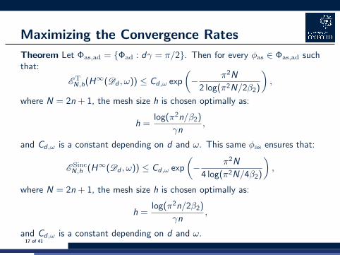
Theorem Let Φas,ad = {Φad : dγ = π/2}. Then for every φas ∈ Φas,ad suchthat:
E TN,h(H∞(Dd , ω)) ≤ Cd,ω exp
(− π2N
2 log(π2N/2β2)
),
where N = 2n + 1, the mesh size h is chosen optimally as:
h =log(π2n/β2)
γn,
and Cd,ω is a constant depending on d and ω. This same φas ensures that:
E SincN,h (H∞(Dd , ω)) ≤ Cd,ω exp
(− π2N
4 log(π2N/4β2)
),
where N = 2n + 1, the mesh size h is chosen optimally as:
h =log(π2n/2β2)
γn,
and Cd,ω is a constant depending on d and ω.17 of 41

Practical Application
Interval Single Exponential Double Exponential
[−1, 1] tanh(t/2) tanh(π2 sinh t)(−∞,+∞) sinh(t) sinh(π2 sinh t)[0,+∞) log(exp(t) + 1) log(exp(π2 sinh t) + 1)[0,+∞) exp(t) exp(π2 sinh t)
The four maps can be written as compositions:
ψ(z) = tanh(z), ψ−1(z) = tanh−1(z),
ψ(z) = sinh(z), ψ−1(z) = sinh−1(z),
ψ(z) = log(ez + 1), ψ−1(z) = log(ez − 1),
ψ(z) = exp(z), ψ−1(z) = log(z).
with the π2 sinh function. Let f have singularities at the points
{δk ± iεk}nk=1. Let {δk ± iεk}nk=1 = {ψ−1(δk ± iεk)}nk=1.18 of 41

Schwarz-Christoffel Formula
sinh maps Dπ2→ C with two branches at ±i.
Let g map the strip Dπ2
to the polygonally bounded region P having
vertices {wk}nk=1 = {δ1 + iε1, . . . , δn + iεn} and interior angles{παk}nk=1. Let also π
2α± be the divergence angles at the left and rightends of the strip Dπ
2. Then the function:
g(z) = A + C
∫ z
e(α−−α+)ζn∏
k=1
[sinh(ζ − zk)]αk−1dζ,
where zk = g(wk) and for some A and C maps the interior of the tophalf of the strip Dπ
2to the interior of the polygon P.
[Hale and Tee 2008] use the Schwarz-Christoffel formula from the unitcircle to maximize convergence rate of Chebyshev methods.
19 of 41
Practical Alternative
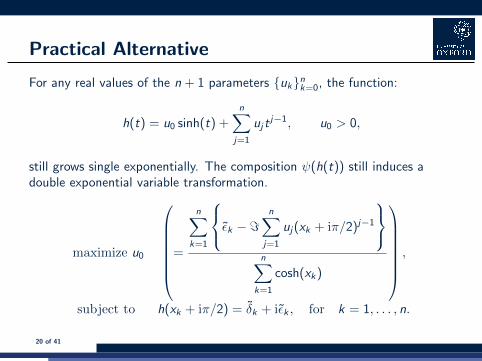
For any real values of the n + 1 parameters {uk}nk=0, the function:
h(t) = u0 sinh(t) +n∑
j=1
uj tj−1, u0 > 0,
still grows single exponentially. The composition ψ(h(t)) still induces adouble exponential variable transformation.
maximize u0
=
n∑k=1
εk −=n∑
j=1
uj(xk + iπ/2)j−1
n∑
k=1
cosh(xk)
,
subject to h(xk + iπ/2) = δk + iεk , for k = 1, . . . , n.
20 of 41

Example: Endpoint and Complex Singularities
∫ 1
−1
exp((ε2
1 + (x − δ1)2)−1)
log(1− x)
(ε22 + (x − δ2)2)
√1 + x
dx = −2.04645 . . . ,
for the values δ1 + iε1 = −1/2 + i and δ2 + iε2 = 1/2 + i/2. This integralhas two different endpoint singularities and two pairs of complex conjugatesingularities of different types near the integration axis.
Single Double Optimized Doubleφ(t) tanh(t/2) tanh
(π2 sinh(t)
)tanh(h(t))
ρ or γ 1 1 1β or β2 1/2 π/4 0.06956
d 1.10715 0.34695 π/2
The optimized transformation is given by:
h(t) ≈ 0.13912 sinh(t) + 0.19081 + 0.21938 t.
21 of 41

Example: Endpoint and Complex Singularities
����
��
����
�
���
�
���
��
�� �� � � �
�
��
��
�
�
�
��
�� ���� � ��� �
�
Dπ2
tanh( 12Dπ
2)
����
��
����
�
���
�
���
��
�� �� � � �
�
����
��
����
�
���
�
���
��
���� ���� ���� ���� � ��� ��� ��� ���
�
��
��
�
�
�
��
�� ���� � ��� �
�
Dπ2
π2
sinh(Dπ2
) tanh(π2
sinh(Dπ2
))
22 of 41

Example: Endpoint and Complex Singularities
����
��
����
�
���
�
���
��
�� �� � � �
�
����
��
����
�
���
�
���
��
���� ���� ���� ���� � ��� ��� ��� ���
�
��
��
�
�
�
��
�� ���� � ��� �
�
Dπ2
g(Dπ2
) tanh(g(Dπ2
))
����
��
����
�
���
�
���
��
�� �� � � �
�
����
��
����
�
���
�
���
��
���� ���� ���� ���� � ��� ��� ��� ���
�
��
��
�
�
�
��
�� ���� � ��� �
�
Dπ2
h(Dπ2
) tanh(h(Dπ2
))
23 of 41

Example: Endpoint and Complex Singularities
���
��
�
�
��
����
�� ���� � ��� �
�
��
��
������������
����
���
���
���
���
�
����������������������
� �� ��� ��� ��� ���
�������
Integrand Error
24 of 41

Obtaining an Initial Guess
Let ε be the smallest of {εk}nk=1 and δ be the δk of the same index. Thenthe nonlinear program with singularities {δ + iεk}nk=1 is exactly solved by:
h(t) = ε sinh t + δ.
A homotopy H (t) is then constructed between {δ + iεk}nk=1 at t = 0 and
{δk + iεk}nk=1 at t = 1.
����
����
����
����
�
���
���
���
���
��
�� �� �� � � � �
�
����
����
����
����
�
���
���
���
���
��
�� �� �� � � � �
�
����
����
����
����
�
���
���
���
���
��
�� �� �� � � � �
�
H (0) H (1/2) H (1)25 of 41

Singularities Unknown
Definition Let xk = kh be the Sinc points and let f (xk) be the N(= 2n + 1)Sinc sampling of f . Then for r + s ≤ 2n, the Sinc-Pade approximants{r/s}f (x) are given by:
{r/s}f (x) =
r∑i=0
pi xi
1 +s∑
j=1
qj xj
,
where the r + s + 1 coefficients solve the system:
r∑i=0
pi xik − f (xk)
s∑j=1
qj xjk = f (xk),
for k = −b r+s2 c, . . . , d
r+s2 e.
26 of 41

Singularities Unknown
Our adaptive algorithm is based on the following principles:
1 Sinc-Pade approximants are useful only when the Sinc approximationobtains some degree of accuracy,
2 Sinc-Pade approximants are useful for r , s = O(log n) as n→∞.
AlgorithmSet n = 1;while |RelativeError| ≥ 10−3 do
Double n and naıvely compute the nth double exponentialapproximation;
end;while |RelativeError| ≥ ε do
Compute the poles of the Sinc-Pade approximant;Solve the nonlinear program for h(t);Double n and compute the nth adapted optimizedapproximation;
end.27 of 41

Adaptive Optimization via Sinc-Pade
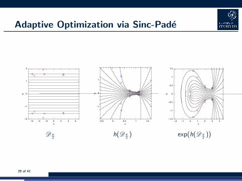
∫ ∞0
x dx√ε2
1 + (x − δ1)2(ε22 + (x − δ2)2)(ε2
3 + (x − δ3)2),
for the values δ1 + iε1 = 1 + i, δ2 + iε2 = 2 + i/2, and δ3 + iε3 = 3 + i/3.
���������
����
�
�
�
�
�
��
����
� � � � �
�
��
��
������������
���������������������
����
���
���
���
���
�
����������������������
� �� ��� ��� ��� ���
�������
28 of 41
Adaptive Optimization via Sinc-Pade
��
��
�
�
�
��
�� �� �� � � � �
�
��
�
�
��
���� � ��� � ���
�
����
��
����
�
���
�
���
��
�� �� � � � � �
�
Dπ2
h(Dπ2
) exp(h(Dπ2
))
29 of 41

Molecular Integrals
Many molecular properties are based on the electronic density.
Molecular structure ⇒ ability to interact with other molecules.
Applications in pharmaceutical industry, efficiency of combustion engines.
The N atom and n electron Schrodinger equation:
Hψ = Eψ,
where:
H =n∑
i=1
−∇2i
2+
N∑A=1
ZA
riA+
n∑i<j
1
rij
.
includes kinetic energy, nuclear attraction, and electron repulsion.
The Born-Oppenheimer approximation ⇒ atoms do not move.
The Pauli exclusion principle ⇒ Slater determinant for wavefunction.
30 of 41

Molecular Integrals
Using a LCAO-MO (Rayleigh-Ritz) approach:
Ψi =∞∑k=1
ckiϕk , i = 1, 2, . . . , n.
We obtain an infinite system of linear equations, whose generalizedeigenvalues approximate the eigenvalues of the i th electron’s Hamiltonian: 〈ϕ1|He |ϕ1〉 〈ϕ1|He |ϕ2〉 · · ·
〈ϕ2|He |ϕ1〉 〈ϕ2|He |ϕ2〉 · · ·...
.... . .
c1i
c2i
...
= Ei
〈ϕ1|ϕ1〉 〈ϕ1|ϕ2〉 · · ·〈ϕ2|ϕ1〉 〈ϕ2|ϕ2〉 · · ·
......
. . .
.
31 of 41

Molecular Integrals
The B functions of [Filter and Steinborn 1978]:
Bmn,l(ζ, ~r) =
(ζr)l
2n+l(n + l)!kn− 1
2(ζr)Ym
l (θ~r , φ~r ),
where n, l , and m are the quantum numbers. Linear combination ofSlater-type orbitals with compact Fourier transform.The three-center nuclear attraction integrals:
In2,l2,m2
n1,l1,m1=
∫ [Bm1
n1,l1(ζ1, ~r)
]∗ 1
|~r − ~R1|Bm2
n2,l2(ζ2, ~r − ~R2)d3~r ,
The four-center two-electron Coulomb integrals:
J n2,l2,m2,n4,l4,m4
n1,l1,m1,n3,l3,m3=
∫ [Bm1
n1,l1(ζ1, ~r)Bm3
n3,l3(ζ3, ~r
′ − ~R34)]∗
1
|~r − ~r ′ − ~R41|Bm2
n2,l2(ζ2, ~r − ~R21)Bm4
n4,l4(ζ4, ~r
′)d3~r d3~r ′,
32 of 41
Molecular Integrals
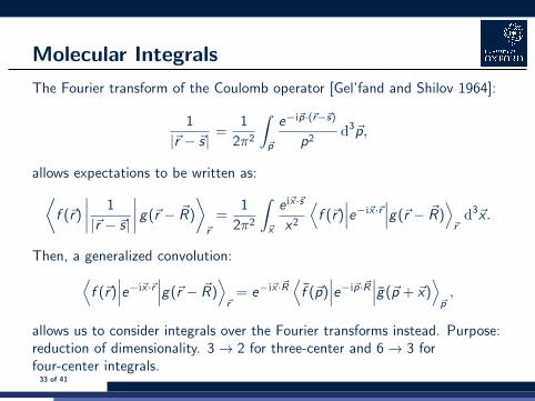
The Fourier transform of the Coulomb operator [Gel’fand and Shilov 1964]:
1
|~r − ~s|=
1
2π2
∫~p
e−i~p·(~r−~s)
p2d3~p,
allows expectations to be written as:⟨f (~r)
∣∣∣∣ 1
|~r − ~s|
∣∣∣∣ g(~r − ~R)
⟩~r
=1
2π2
∫~x
ei~x·~s
x2
⟨f (~r)
∣∣∣e−i~x·~r ∣∣∣g(~r − ~R)⟩~rd3~x .
Then, a generalized convolution:⟨f (~r)
∣∣∣e−i~x·~r ∣∣∣g(~r − ~R)⟩~r
= e−i~x·~R⟨f (~p)
∣∣∣e−i~p·~R ∣∣∣g(~p + ~x)⟩~p,
allows us to consider integrals over the Fourier transforms instead. Purpose:reduction of dimensionality. 3→ 2 for three-center and 6→ 3 forfour-center integrals.
33 of 41
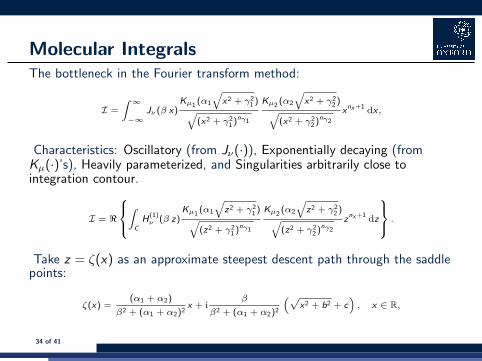
Molecular IntegralsThe bottleneck in the Fourier transform method:
I =
∫ ∞−∞
Jν(β x)Kµ1
(α1
√x2 + γ2
1 )√(x2 + γ2
1 )nγ1
Kµ2(α2
√x2 + γ2
2 )√(x2 + γ2
2 )nγ2
xnx +1dx,
Characteristics: Oscillatory (from Jν(·)), Exponentially decaying (fromKµ(·)’s), Heavily parameterized, and Singularities arbitrarily close tointegration contour.
I = <
∫C
H(1)ν (β z)
Kµ1(α1
√z2 + γ2
1 )√(z2 + γ2
1 )nγ1
Kµ2(α2
√z2 + γ2
2 )√(z2 + γ2
2 )nγ2
znx +1dz
.
Take z = ζ(x) as an approximate steepest descent path through the saddlepoints:
ζ(x) =(α1 + α2)
β2 + (α1 + α2)2x + i
β
β2 + (α1 + α2)2
(√x2 + b2 + c
), x ∈ R,
34 of 41
Molecular Integrals
35 of 41

Molecular Integrals
36 of 41

Molecular Integrals
Consider the integral:∫ +∞
−∞
ei b z−a1
√z2+c2
1−a2
√z2+c2
2
(z2 + c21 )µ1 (z2 + c2
2 )µ2dz ,
for positive real parameter values. To remove oscillations, we deform theintegration contour to a path of steepest descent. We use an asymptoticpath of steepest descent parameterized by:
ζ(x) = λ1x + i
(√λ2
2x2 + λ2
3 + λ4
),
for some values of the parameters λ. From horizontal and vertical symmetry,we can use:
h(t) = u0 sinh(t) + u2 t.
37 of 41

Molecular Integrals
20 runs with randomized values for the parameters distributed uniformly:
a1 ∼ U(0, 1), a2 ∼ U(0, 1), b ∼ U(0, 20),c1 ∼ U(0, 1), c2 ∼ U(0, 2), µ1 ∼ U(0, 1), µ2 ∼ U(0, 1).
��
���
���
���
���
���
�
����������������������
� �� �� �� �� ��� ���
�������
��
���
���
���
���
���
�
����������������������
� �� �� �� �� ��� ���
�������
������������
���
���
���
���
���
�
����������������������
� �� �� �� �� ��� ���
�������
SE DE Optimized DE
38 of 41

Conclusions & Outlook
Conformal maps maximize the convergence rates of trapezoidal rule andSinc numerical methods (subject to their very existence!)
Practical & general solution as a polynomial adjustment to sinh map
Sinc-Pade approximants for unknown singularities
Free & open-source implementation available in the Julia softwarepackage DEQuadrature.jl
Will polynomial adjustments (in the monomial basis) to the sinh map standthe test of time? There is lots to explore:
sinh +polynomial in a Chebyshev basis
sinh + rational approximant
Potential-theoretic approach to interpolatory nodes and weights on thewhole real line
shortest enclosing walks to find optimal contours for Cauchy integrals[Bornemann and Wechslberger 2012]
39 of 41

Acknowledgements
Special thanks to:
Hassan Safouhi (PhD supervisor)
Sheehan Olver (host supervisor at The University of Sydney)
Tomoaki Okayama (invitation to UTNAS)
Norikazu Saito (organizer of UTNAS)
Financial support:
The Natural Sciences and Engineering Research Council ofCanada (NSERC)
Alexander Graham Bell Canada Graduate Scholarship 2011 – 2014Michael Smith Foreign Study Scholarship 2014Postdoctoral Fellowship 2014 – 2016
The University of Alberta’s Faculty of Graduate Studies & Research
Thank you all very much for your time!
40 of 41

References
1 F. Bornemann and G. Wechslberger. IMA J. Numer. Anal., online, 2012.
2 E. Filter and E.O. Steinborn. Phys. Rev. A., 18:1–11, 1978.
3 I. M. Gel’fand and G. E. Shilov. Academic Press, New York, 1964.
4 N. Hale and T. W. Tee. SIAM J. Sci. Comput., 31:3195–3215, 2009.
5 M. Mori. RIMS, 41:897–935, 2005.
6 H. Safouhi. J. Phys. A: Math. Gen., 34:2801–2818, 2001.
7 H. Safouhi. J. Comp. Phys., 176:1–19, 2002.
8 F. Stenger. J. Inst. Math. Appl., 12:103–114, 1973.
9 M. Sugihara. Numerische Mathematik, 75:379–395, 1997.
10 M. Sugihara. Math. Comp., 72:767–786, 2003.
11 H. Takahasi and M. Mori. RIMS, 9:721–741, 1974.
12 L. N. Trefethen and J. A. C. Weideman, SIAM Rev., 56:385–458, 2014.
41 of 41

![Computing Harmonic Maps and Conformal Maps on Point …...There is an extensive literature on computing conformal maps for triangle meshes. Gu-Yau [24][25] developed the method of](https://img.dokumen.tips/doc/110x75/6026bd2bacadd15b9b79a662/computing-harmonic-maps-and-conformal-maps-on-point-there-is-an-extensive-literature.jpg)