On the tree-transformation power of XSLT

Wim Janssen Alexandr Korlyukov� Jan Van den Bussche∗

Abstract

XSLT is a standard rule-based programming language for express-ing transformations of XML data. The language is currently in tran-sition from version 1.0 to 2.0. In order to understand the computa-tional consequences of this transition, we restrict XSLT to its puretree-transformation capabilities. Under this focus, we observe thatXSLT 1.0 was not yet a computationally complete tree-transformationlanguage: every 1.0 program can be implemented in exponential time.A crucial new feature of version 2.0, however, which allows node setsover temporary trees, yields completeness. We provide a formal opera-tional semantics for XSLT programs, and establish confluence for thissemantics.

1 Introduction

XSLT is a powerful rule-based programming language, relatively widelyused, for expressing transformations of XML data, and is developed by theW3C (World Wide Web Consortium) [2, 8, 17]. An XSLT program is runon an XML document as input, and produces another XML document asoutput. (XSLT programs are actually called “stylesheets”, as one of theirmain uses is to produce stylised renderings of the input data, but we willcontinue to call them programs here.)

The language is actually in a transition period: the current standard,version 1.0, is being replaced by version 2.0. It is important to understandwhat the new features of 2.0 really add. In the present paper, we focus onthe tree-transformation capabilities of XSLT. Indeed, XML documents areessentially ordered, node-labeled trees.

∗Wim Janssen and Jan Van den Bussche are with the University of Hasselt, Belgium.Alexandr Korlyukov, who was with Grodno State University, Belarus, sadly passed

away shortly after we agreed to write a joint paper.

1

From the perspective of tree-transformation capabilities, the most im-portant new feature is that of “node sets over temporary trees”. We willshow that this feature turns XSLT into a computationally complete tree-transformation language. Indeed, as we will also show, XSLT 1.0 was notyet complete in this sense. Specifically, any 1.0 program can be implementedwithin exponential time in the worst case. Some programs actually expressPSPACE-complete problems, because we will show that any linear-spaceturing machine can be simulated by an XSLT 1.0 program.

To put our results in context, we note that the designers of XSLT willmost probably regard the incompleteness of their language as a feature,rather than a defect. Indeed, in the requirements document for 2.0, turningXSLT into a general-purpose programming language is explicitly stated as a“non-goal” [3]. In that respect, our result on the completeness of 2.0 exposes(albeit in a narrow sense) a failure to meet the requirements!

At this point we should be a little clearer on what we mean by “focusingon the tree-transformation capabilities of XSLT”. As already mentioned,XML documents are essentially trees where the nodes are labeled by ar-bitrary strings. We make abstraction of this string content by regardingthe node labels as coming from some finite alphabet. Accordingly, we stripXSLT of its string-manipulation functions, and restrict its arithmetic toarbitrary polynomial-time functions on counters, i.e., integers in the range{1, 2, . . . , n} with n the number of nodes in the input tree. It is, incidentally,quite easy to see that XSLT 1.0 without these restrictions can express allcomputable functions on strings (or integers). Indeed, rules in XSLT can becalled recursively, and we all know that arbitrary recursion over the stringsor the integers gives us completeness.

We will provide a formal operational semantics for the substantial frag-ment of XSLT discussed in this paper. A formal semantics has not beenavailable, although the W3C specifications represent a fine effort in definingit informally. Of course we have tried to make our formalisation faithful tothose specifications. Our semantics does not impose an order on operationswhen there is no need to, and as a result the resulting transition relationis non-deterministic. We establish, however, a confluence property, so thatany two terminating runs on the same input yield the same final result.Confluence was not yet proven rigorously for XSLT, and can help in pro-viding a formal justification for alternative processing strategies that XSLTimplementations may follow for the sake of optimisation.

2

a

b c

a b

c

Figure 1: A data tree.

2 Data model

2.1 Data trees

Let Σ be a finite alphabet, including the special label doc. By a data treewe simply mean a finite ordered tree, in which the nodes are labeled byelements of Σ. Up to isomorphism, we can describe a data tree t by a stringstring(t) over the alphabet Σ extended with the two symbols { and }: if theroot of t is labeled a and its sequence of top-level subtrees is t1, . . . , tk, then

string(t) = a{string(t1) . . . string(tk)}

Thus, for the data tree shown in Figure 1, the string representation equals

a{b{}c{a{}b{}}c{}}.

A data forest is a finite sequence of data trees. Forests arise naturallyin XSLT, and for uniformity reasons we need to be able to present them asdata trees. This can easily be done as follows:

Definition 1 (maketree). Let F be a data forest. Then maketree(F ) isthe data tree obtained by affixing a root node on top of F , and labeling thisroot node with doc.1

2.2 Stores and values

Let T be a supply of tree variables, including the special tree variable Input.We define:

1The root node added by maketree models what is called the “document root” in theXPath data model [6], although we do not model it entirely faithfully, as we do not formallydistinguish “document nodes” from “element nodes”. This is only for simplicity; it is noproblem to incorporate this distinction in our formalism, and our technical results do notdepend on our simplification.

3

Definition 2. A store is a finite set S of pairs of the form (x, t), wherex ∈ T and t is a data tree, such that (1) Input occurs in S; (2) no treevariable occurs twice in S; and (3) all data trees occurring in S have disjointsets of nodes.

The tree assigned to Input is called the input tree; the other trees arecalled the temporary trees.

Definition 3. A value over S is a finite sequence consisting of nodes fromtrees in S, and counters over S. Here, a counter over S is an integer in therange {1, 2, . . . , n}, where n is the total number of nodes in S.

Values as defined above formalise the kind of values that can be returnedby XPath expressions. XPath [1, 5] is a language that is used as a sublan-guage in XSLT for the purpose of selecting nodes from trees. But XPathexpressions can also return numbers, which is useful as an aid in makingnode selections (e.g., the i-th child of a node, or the i-th node of the tree inpreorder). We limit these numbers to counters, in order to concentrate onpure tree transformations.

3 XPath abstraction

Since the language XPath is already well understood [27, 13, 7, 14], andits study in itself is not our focus, we will work with an abstraction ofXPath, which we denote by X . For our purposes it will suffice to divide theX -expressions in only two different types, which we denote by nodes andmixed. A value is of type nodes if it consists exclusively of nodes; otherwiseit is of type mixed.

In order to define the semantics of X , we need some definitions, whichreflect those from the XPath specification. Let V be a supply of valuevariables, disjoint from T .

Definition 4. An environment over S is a finite set E of pairs of the form(x, v), where x ∈ V and v is a value over S, such that no value variableoccurs twice in E.

Definition 5. A context triple over S is a triple (z, i, k) where z is a nodefrom S or a counter over S, and i and k are counters over S such that i � k.We call z the context item, i the context position, and k the context size.

Definition 6. A context is a triple (S,E, c) where S is a store, E is anenvironment over S, and c is a context triple over S.

4

If we denote the universe of all possible contexts by Contexts, the se-mantics of X is now given by a partial function eval on X ×Contexts , suchthat whenever defined, eval(e,C) is a value over C’s store, and this valuehas the same type as e.

Remark 3.1. A static type system, based on XML Schema [4, 25], can beput on contexts to ensure definedness of expressions [7], but we omit thatas safety is not the focus of the present paper.

In general we do not assume much from X , except for the availability ofthe following basic expressions, also present in real XPath:

• An expression ‘/*’, such that eval(/*, C) equals the root node of theinput tree in C’s store.

• An expression ‘child::*’, such that eval(child::*, C) is defined when-ever C’s context item is a node n, and then equals the list of childrenof n.

4 Syntax

In this section, we define the syntax of a sizeable fragment of XSLT 2.0. Thereader familiar with XSLT will notice that we have simplified and cleanedup the language in a few places. These modifications are only for the sakeof simplicity of exposition, and our technical results do not depend on them.We discuss our deviations from the real language further in Section 5.5.

Also, the concrete syntax of real XSLT is XML-based and rather un-wieldy. For the sake of presentation, we therefore give a syntax of our own,which is non-XML, but otherwise follows the same lines as the real syntax.

The grammar is shown in Figure 2. The only typing condition we needis that in an apply-statement or in a vcopy-statement, expr must be of typenodes. Also, no two different rules can have the same name, and the namein a call-statement must be the name of some rule.

We will often identify a template M with its syntax tree. This tree con-sists of all occurrences of statements in M and represents how they followeach other and how they are nested in each other; we omit the formal defi-nition. Observe that only cons-, foreach-, tree-, and if-statements can havechildren. Note also that, since a template is a sequence of statements, thesyntax “tree” is actually a forest, i.e., a sequence of trees, but we will stillcall it a tree.

5

Program → Rule*Rule → template name match expr (mode name)? { Template }Template → Statement*Statement → cons label { Template }

| apply expr (mode name)?| call name| foreach expr { Template }| val value variable expr| tree tree variable { Template }| vcopy expr| tcopy tree variable| if expr { Template } else { Template }

Figure 2: Our syntax. The terminal symbol expr stands for an X -expression; label stands for an element of our alphabet Σ; value variableand tree variable stand for elements of V and T , respectively; and nameis self-explanatory. As usual we use * to denote repetition, ? to denoteoptionality, and use ( and ) for lexical grouping.

Variable definitions happen through val- and tree-statements. We willneed the notion of a statement being in the scope of some variable definition;this is defined in the standard way as follows.

Definition 7. Let M be a template, and let S1 and S2 be two statementsoccurring in M . We say that S2 is in the scope of S1 if S2 is a right siblingof S1 in the syntax tree of M , or a descendant of such a right sibling. Anillustration is in Figure 3.

One final definition:

Definition 8. Template M ′ is called a subtemplate of template M if M ′

consists of a sequence of consecutive sibling statements occurring in M .

5 Operational semantics

Fix a program P and a data tree t. We will describe the semantics of P oninput t as a rewrite relation ⇒ among configurations.

Definition 9. A configuration consists of a template M together with apartial function that assigns a context to some of the statements of M (more

6

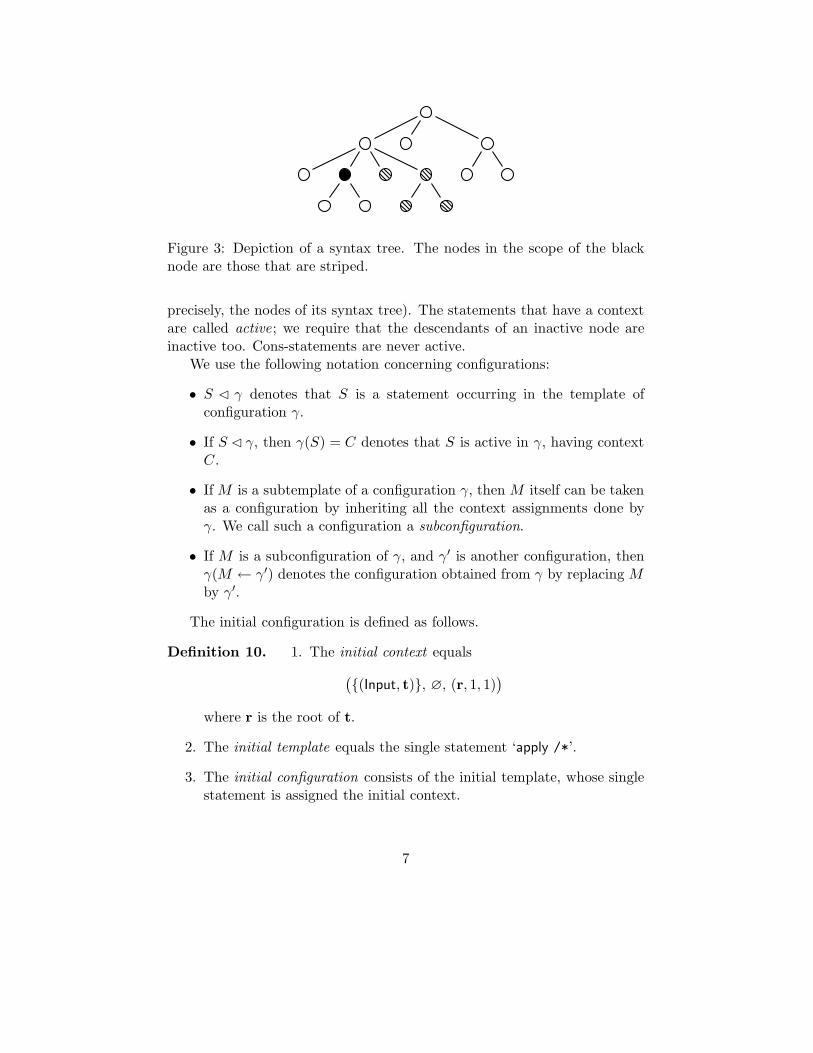
Figure 3: Depiction of a syntax tree. The nodes in the scope of the blacknode are those that are striped.

precisely, the nodes of its syntax tree). The statements that have a contextare called active; we require that the descendants of an inactive node areinactive too. Cons-statements are never active.

We use the following notation concerning configurations:

• S � γ denotes that S is a statement occurring in the template ofconfiguration γ.

• If S � γ, then γ(S) = C denotes that S is active in γ, having contextC.

• If M is a subtemplate of a configuration γ, then M itself can be takenas a configuration by inheriting all the context assignments done byγ. We call such a configuration a subconfiguration.

• If M is a subconfiguration of γ, and γ′ is another configuration, thenγ(M ← γ′) denotes the configuration obtained from γ by replacing Mby γ′.

The initial configuration is defined as follows.

Definition 10. 1. The initial context equals({(Input, t)}, ∅, (r, 1, 1)

)

where r is the root of t.

2. The initial template equals the single statement ‘apply /*’.

3. The initial configuration consists of the initial template, whose singlestatement is assigned the initial context.

7

• S = if e { Mtrue } else { Mfalse } � γγ(S) = Ceval(e,C) �= ∅

γif⇒ γ(S ← Mtrue)

• S = if e { Mtrue } else { Mfalse } � γγ(S) = Ceval(e,C) = ∅

γif⇒ γ(S ← Mfalse)

Figure 4: Semantics of if-statements; ∅ denotes the empty sequence.

The goal will be to rewrite the initial configuration into a terminal tem-plate; this is a configuration consisting exclusively of cons-statements. Ob-serve that terminal templates can be viewed as data forests; indeed, simplyby removing the cons’s from a terminal template, we obtain the string rep-resentation of a data forest.

For the rewrite relation ⇒ we are going to define, terminal configurationswill be normal forms, i.e., cannot be rewritten further. If, for two configura-tions γ0 and γ1, we have γ0 ⇒ · · · ⇒ γ1 and γ1 is a normal form, we denotethat by γ0 ⇒! γ1. The relation ⇒ will be defined in such a way that if γ0 isthe initial configuration and γ0 ⇒! γ1, then γ1 will be terminal. Moreover,we will prove in Theorem 1 that each configuration γ0 has at most one suchnormal form γ1. We thus define:

Definition 11. Given P and t, let γ0 be the initial configuration and letγ0 ⇒! γ1. Then the final result tree of applying P to t is defined to bemaketree(γ1).

In the above definition, we can indeed apply maketree , defined on dataforests (Definition 1), to γ1, since γ1 is terminal and we just observed thatterminal templates describe forests. Note that the final result tree is onlydetermined up to isomorphism.

5.1 If-statements

If-statements are the only ones that generate control flow, so we treat themby a separate rewrite relation if⇒, defined by the semantic rules shown inFigure 4.

8

It is not difficult to show that if⇒ is terminating and locally confluent,whence confluent, so that every configuration has a unique normal formw.r.t. if⇒ [26]. This normal form no longer contains any active if-statements.(Quite obviously, the most efficient way to get to this normal form is to workout the if-statements top-down.) We write γ

if⇒ ! γ′ to denote that γ′ is thenormal form of γ w.r.t. if⇒.

Remark 5.1. Our main rewrite relation ⇒ is not terminating in general.The reason why we treat if-statements separately is to avoid nonsensicalrewritings such as where we execute a non-terminating statement in theelse-branch of an if-statement whose test evaluates to true.

5.2 Apply-, call-, and foreach-statements

For the semantics of apply-statements, we need the following definitions.

Definition 12 (ruletoapply). Let C be a context, let n be a node, and letm be a name. Then ruletoapply(C,n) (respectively, ruletoapply(C,n,m))equals the template belonging to the first rule in P (respectively, with modename equal to m) whose expr satisfies n ∈ eval(expr, C).

If no such rule exists, both ruletoapply(C,n) and ruletoapply(C,n,m)default to the single-statement template ‘apply child::*’.

Definition 13 (init). Let M be a template, and let C be a context. Theninit(M,C) equals the configuration obtained from M by assigning contextC to every statement in M , except for all statements in the scope of anyvariable definition, and all statements that are below a foreach-statement;all those statements remain inactive.

We are now ready for the semantic rule for apply-statements, shown inFigure 5. We omit the rule for an apply-statement with a mode m: the onlydifference with the rule shown is that we use ruletoapply(ni, C,m).

The semantic rule for foreach-statements is very similar to that for apply-statements, and is also shown in Figure 5.

For call-statements, we need the following definition.

Definition 14 (rulewithname). For any name, let rulewithname(name)denote the template of the rule in P with that name.

The semantic rule for a call-statement is then again shown in Figure 5.

9

• S = apply e � γγ(S) = C = (S,E, c)eval(e,C) = (n1, . . . ,nk)ruletoapply(ni, C) = Mi for i = 1, . . . , kinit(Mi, (S,E, (ni, i, k))) = γi for i = 1, . . . , k

γ(S ← γ1 . . . γk)if⇒ ! γ′

γ ⇒ γ′

• S = foreach e { M } � γγ(S) = C = (S,E, c)eval(e,C) = (z1, . . . , zk)init(M, (S,E, (zi, i, k))) = γi for i = 1, . . . , k

γ(S ← γ1 . . . γk)if⇒ ! γ′

γ ⇒ γ′

• S = call name � γγ(S) = Crulewithname(name) = Minit(M,C) = γ1

γ(S ← γ1)if⇒ ! γ′

γ ⇒ γ′

Figure 5: Semantics of apply-, call-, and foreach-statements.

10

• S = val x e � γγ(S) = CC(x : eval(e,C)) = C ′

updateset(γ, S) = Minit(M,C ′) = γ1

γ(SM ← γ1)if⇒ ! γ′

γ ⇒ γ′

• S = tree y { M } � γM is terminalγ(S) = CC(y : maketree(M)) = C ′

updateset(γ, S) = M ′

init(M ′, C ′) = γ3

γ(SM ′ ← γ3)if⇒ ! γ′

γ ⇒ γ′

Figure 6: Semantics of variable definitions.

5.3 Variable definitions

For a context C = (S,E, c), a value variable x, a value v, a tree variable y,and a data tree t, we denote by

• C(x : v) the context obtained from C by updating E with the pair(x, v); and by

• C(y : t) the context obtained from C by updating S with the pair(y, t).

We also define:

Definition 15 (updateset). Let γ be a configuration and let S � γ. LetM be the template underlying γ. Let S1, . . . , Sk be the right siblings of Sin M , in that order. Let j be the smallest index for which Sj is active inγ; if all the Si are inactive, put j = k + 1. Then the template S1 . . . Sj−1 isdenoted by updateset(γ, S). If j = 1 then this is the empty template.

We are now ready for the semantic rules for variable definitions, shownin Figure 6.

11

a

b n1 c n2

a n3 b

c

c n4

a b

ttemp(forest((n4,n1,n2,n3,n1),S)

)= cons c { cons a {} cons b {} }

cons b {}cons c { cons a {} cons b {} }cons a {}cons b {}

Figure 7: Illustration of Definitions 16 and 17.

5.4 Copy-statements

The following definitions are illustrated in Figure 7.

Definition 16 (forest). Let S be a store, and let (n1, . . . ,nk) be a sequenceof nodes from S. For i = 1, . . . , k, let ti be the data subtree rooted at ni.Then forest((n1, . . . ,nk),S) equals the data forest (t1, . . . , tn).

Definition 17 (ttemp). Let F be a data forest. Then ttemp(F ) equalsthe terminal template describing F .

We also need:

Definition 18 (choproot). Let t be a data tree with top-level subtreest1, . . . , tk, in that order. Then choproot (t) equals the data forest (t1, . . . , tk).

The semantic rules for copy-statements are now shown in Figure 8.

5.5 Discussion

The final result of applying P to t (Definition 11) may be undefined for twovery different reasons. The first, fundamental, reason is that the rewritingmay be nonterminating. The second reason is that the rewriting may abortbecause the evaluation of an X -expression is undefined, or the tree variable ina tcopy-statement is not defined in the store. This second reason can easilybe avoided by a type system on X , as already mentioned in Remark 3.1,together with scoping rules to keep track of which variables are visible inthe XSLT program and which variables are used in the X -expressions. Such

12

• S = vcopy e � γγ(S) = C = (S,E, c)eval(e,C) = (n1, . . . ,nk)ttemp

(forest((n1, . . . ,nk),S)

)= M

γ ⇒ γ(S ← M)

• S = tcopy y � γγ(S) = (S,E, c)(y, t) ∈ Sttemp(choproot (t)) = M

γ ⇒ γ(S ← M)

Figure 8: Semantics of copy-statements.

scoping rules are entirely standard, and indeed are implemented in the XSLTprocessor SAXON [16].

In the same vein, we have simplified the parameter passing mechanismof XSLT, and have omitted the feature of global variables. On the otherhand, our mechanism for choosing the rule to apply (Definition 12) is morepowerful than the one provided by XSLT, as ours is context-dependent. Itis actually easier to define that way. As already mentioned at the beginningof Section 4, none of our technical results depend on the modifications wehave made.

Finally, we note that the XSLT processor SAXON evaluates variabledefinitions lazily, whereas we simply evaluate them eagerly. Again, lazyevaluation could have been easily incorporated in our formalism. Someprograms may terminate on some inputs lazily, while they do not terminateeagerly, but for programs that use all the variables they define there is nodifference.

5.6 Confluence

Recall that we call a rewrite relation confluent if, whenever we can rewritea configuration γ1 to γ2 as well as to γ3, then there exists γ4 such thatwe can further rewrite both γ2 and γ3 into γ4. Confluence guarantees thatall terminating runs from a common configuration also end in a commonconfiguration [26]. Since, for our rewrite relation ⇒, either all runs on someinput are nonterminating, or none is, the following theorem implies that thesame final result of a program P on an input t, if defined at all, will be

13

obtained regardless of the order in which we process active statements.

Theorem 1. Our rewrite relation ⇒ is confluent.

Proof. The proof is a very easy application of a basic theorem of Rosenabout subtree replacement systems [24]. A subtree replacement system Ris a (typically infinite) set of pairs of the form φ → ψ, where φ and ψare descriptions up to isomorphism of ordered, node-labeled trees, wherethe node labels come from some (again typically infinite) set V . Let usrefer to such trees as V -trees. Such a system R naturally induces a rewritesystem ⇒R on V -trees: we have t ⇒R t′ if there exists a node n of tand a pair φ → ψ in R such that the subtree t/n is isomorphic to φ, andt′ = t(n ← ψ). Here, we use the notation t/n for the subtree of t rooted atn, and the notation t(n ← ψ) for the tree obtained from t by replacing t/nby a fresh copy of ψ. Rosen’s theorem states that if R is “unequivocal” and“closed”, then ⇒R is confluent.

“Unequivocal” means that for each φ there is at most one ψ such thatφ → ψ is in R. The definition of R being “closed” is a bit more complicated.To state it, we need the notion of a residue map from φ to ψ. This is amapping r from the nonroot nodes of φ to sets of nonroot nodes of ψ, suchthat for m ∈ r(n) the subtrees φ/n and ψ/m are isomorphic. Moreover, ifn1 and n2 are independent (no descendants of each other), then all nodes inr(n1) must also be independent of all nodes in r(n2).

Now R being closed means that we can assign a residue map r[φ,ψ]to every φ → ψ in R in such a way that for any φ0 → ψ0 in R, andany node n of φ0, if there exists a pair φ0/n → ψ in R, then the pairφ0(n ← ψ) → ψ0(r[φ0, ψ0](n) ← ψ) is also in R. Denoting the latter pair byφ1 → ψ1, we must moreover have for each node p of φ0 that is independentof n, that r[φ1, ψ1](p) = r[φ0, ψ0](p).

To apply Rosen’s theorem, we view configurations (Definition 9) as V -trees, where V = Statements ∪ (Statements × Contexts). Here, Statementsis the set of all possible syntactic forms of statements. So, given a configu-ration, we take the syntax tree of the underlying template, and label everyinactive node by its corresponding statement, and every active node by itscorresponding statement and its context in the configuration. (Since tem-plates are sequences, we actually get V -forests rather than V -trees, but thatis a minor fuss.)

Now consider the subtree replacement system R consisting of all pairsγ → γ′ for which γ ⇒ γ′ as defined by our semantics, where γ consistsof a single statement S0, and the active statement being processed to getγ′ is a direct child of S0. Since our semantics always substitutes siblings

14

for siblings, it is clear that ⇒R then coincides with our rewrite relation ⇒.Since the processing of every individual statement is always deterministic(up to isomorphism of trees), R as just defined is clearly unequivocal.

We want to show that R is closed. Thereto, we define residue mapsr[γ, γ′] as follows.

The case where γ → γ′ is the processing of an apply- or call-statement,is depicted in Figure 9 (top). The node being processed is shown in black.The subtemplates to the left and right are left untouched. Referring to thenotation used in Figure 5, the newly substituted subtemplate γnew is suchthat γ1 . . . γk

if⇒ ! γnew (for apply) or γ1if⇒ ! γnew (for call). Indeed, since we

apply if⇒ ! at the end of every processing step, γ itself does not contain anyactive if-statements. We define r = r[γ, γ′] as follows:

• For nodes n in γleft or γright, we put r(n) := {n′}, where n′ is thecorresponding node in γ′.

• For the black node b, we put r(b) := ∅.

The main condition for closedness is clearly satisfied, because statementscan be processed independently. Note that the black node has no children,let alone active children, which allows us to put r(b) = ∅. The condition onp’s is also satisfied, because both r[φ0, ψ0] and r[φ1, ψ1] will set r(p) to {p′}.

The case where γ → γ′ is the processing of a foreach-statement is de-picted in Figure 9 (middle). This case is analogous to the previous one.The only difference is that the black node now has descendants (M in thefigure). Because the init function (Definition 13) always leaves descendantsof a foreach node inactive, however, the nodes in M are inactive at this time,and we can put r(n) := ∅ for all of them.

The case where γ → γ′ is the processing of a val-statement is depictedin Figure 9 (bottom). Since all nodes in the update set are inactive bydefinition (Definition 15), we can again put r(n) := ∅ for all nodes in theupdate set. The case of a tree-statement is similar; now the black nodeagain has descendants, but again these are all inactive (they are all cons-statements). The case where γ → γ′ is the processing of a copy-statement,finally, is again analogous.

6 Computational completeness

As defined in Definition 11, an XSLT program P expresses a partial functionfrom data trees to data forests, where the output forest is represented by a

15

γ

γleft

apply/call

γright

→γ′

γleft γnew γright

γ

γleft foreach

M

γright

→γ′

γleft γnew γright

γ

γleft

val

updateset γright

→γ′

γleft γnew γright

Figure 9: Illustration to the proof of Theorem 1.

tree by affixing a root node labeled doc on top (Definition 1). The outputis defined up to isomorphism only, and P does not distinguish betweenisomorphic inputs. This leads us to the following definition:

Definition 19. A tree transformation is a partial function from data treesto data trees with root labeled doc, mapping isomorphic trees to isomorphictrees.

Using the string representation of data trees defined in Section 2.1, wefurther define:

Definition 20. A tree transformation f is called computable if the stringfunction f : string(t) �→ string(f(t)) is computable in the classical sense.

Up to now, we have assumed from our XPath abstraction X only theavailability of the expressions ‘/*’ and ‘child::*’. For our proof of thefollowing theorem, we need to assume the availability of a few more verysimple expressions, also present in real XPath:

• y/*, for any tree variable y, evaluates to the root of the tree assignedto y.

16

• //* evaluates to the sequence of all nodes in the store (it does notmatter in which order).

• child::*[1] evaluates to the first child of the context item (whichshould be a node).

• following-sibling::*[1] evaluates to the immediate right siblingof the context node, or the empty sequence if the context node has noright siblings.

• Increment, decrement, and test on counters: the constant expression‘1’, and the expressions ‘x+1’, ‘x-1’, and ‘x=1’ for any value variable x,which should consist of a single counter. If x has the maximal countervalue, then x+1 need not be defined, and if x has value 1, then x-1need not be defined. The test x=1 yields any nonempty sequence fortrue and the empty sequence for false.

• name()=’a’, for any a ∈ Σ, returning any nonempty sequence if thelabel of the context node is a, and the empty sequence otherwise.

• () evaluates to the empty sequence.

We establish:

Theorem 2. Every computable tree transformation f can be realised by aprogram.

Proof. We can naturally represent any string s over some finite alphabet as aflat data tree over the same alphabet. We denote this flat tree by flattree(s).Its root is labeled doc, and has k children, where k is the length of s, suchthat the labels of the children spell out the string s. There are no othernodes.

The proof now consists of three parts:

1. Program the transformation t �→ flattree(string(t)).

2. Show that every turing machine (working on strings) can be simulatedby some program working on the flattree representation of strings.

3. Program the transformation flattree(string(t)) �→ t.

The theorem then follows by composing these three steps, where we simu-late a turing machine for f in step 2. Note that the composition of threeprograms can be written as a single program, using a temporary tree to

17

template tree2string match (//*){

cons a { }cons lbrace { }apply (child::*)cons rbrace { }

}

Figure 10: From t to flattree(string(t)).

pass the intermediate results, and using modes to keep the rules from thedifferent programs separate.

The programs for steps 1 and 3 are shown in Figures 10 and 11. Forsimplicity, they are for an alphabet consisting of a single letter a, but it isobvious how to generalise the programs. The real XSLT versions are given inthe Appendix. We point out that these programs are actually 1.0 programs,so it is only for step 2 of the proof that we need XSLT 2.0.

For step 2, we can represent a configuration of a turing machine A by twotemporary trees left and right. At each step, variable right holds (as aflat tree) the content of the tape starting at the head position and ending inthe last tape cell; variable left holds the reverse of the tape portion left ofthe head position. To keep track of the current state of the machine, we usevalue variables q for each state q of A, such that at each step precisely oneof these is nonempty. (This is why we need the X -expression ().) Changingthe symbol under the head to an a amounts to assigning a new contentto right by putting in cons a {}, followed by copies of the nodes in thecurrent content of right, where we skip the first one. Moving the head acell to the right amounts to assigning a new content to left by putting in anode labeled with the current symbol, followed by copies of the nodes in thecurrent content of left. We also assign a new content to right in the nowobvious way; if we were at the end of the tape we add a new node labeledblank. Moving the head a cell to the left is simulated analogously. The onlyX -expressions we need here are the ones we have assumed to be available.

The simulation thus consists of repeatedly calling a big if-then-else thattests for the transition to be performed, and performs that transition. Wemay assume A is programmed in such a way that the final output is producedstarting from a designated state. In this way we can build up the final outputstring in a fresh temporary tree and pass it to step 3.

18

template doc match (/*){

apply (child::*[1])}

template string2tree match (//*){

cons a{ apply (following-sibling::*[1]) mode dochildren }val counter (1)call searchnextsibling

}

template dochildren match (//*) mode dochildren{

if name()=’lbrace’{ apply (following-sibling::*[1]) mode dochildren }else {

if name()=’a’{ call string2tree }else { }

}}

template searchnextsibling match (//*) mode search{

if name()=’lbrace’ {val counter (counter + 1)apply (following-sibling::*[1]) mode search

}else {

if name()=’a’{ apply (following-sibling::*[1]) mode search }else {

val counter (counter - 1)if counter = 1{ apply (following-sibling::*[1])

mode dochildren }else{ apply (following-sibling::*[1]) mode search }

}}

}

Figure 11: From flattree(string(t)) to t.

19

7 XSLT 1.0

In this section we will show that every XSLT 1.0 program can be imple-mented in exponential time, in sharp contrast to the computational com-pleteness result of the previous section.

A fundamental difference between XSLT 1.0 and 2.0 is that in 1.0, X -expressions are “input-only”, defined as follows.

Definition 21. 1. Let C = (S,E, (z, i, k)) be a context. Let the inputtree in S be t. Then we call C input-only if every value appearing inE is already a value over the store {(Input, t)}, and also (z, i, k) is likethat.

2. By C, we mean the context ({(Input, t)},E, (z, i, k)). So, C equals Cwhere we have removed all temporary trees.

3. Now an X -expression e is called input-only if for any input-only contextC for which eval(e,C) is defined, we have eval(e,C) = eval(e, C), andthis must be a value over C’s input tree only.

In other words, input-only expressions are oblivious to the temporarytrees in the store; they only see the input tree.

We further define:

Definition 22. An input-only X -expression e is called polynomial if foreach input-only context C, the computation of eval(e,C) can be done intime polynomial in the size of C’s input tree.

We now define:

Definition 23. A program is called 1.0 if it only uses input-only, polynomialX -expressions.

Essentially, 1.0 programs cannot do anything with temporary trees ex-cept copy them using tcopy statements. We note that real XPath 1.0 ex-pressions are indeed input-only and polynomial; actually, real XPath 1.0is much more restricted than that, but for our purpose we do not need toassume anything more.

In order to establish an exponential upper bound on the time-complexityof 1.0 programs, we cannot use an explicit representation of the output tree.Indeed, 1.0 programs can produce result trees of size doubly exponentialin the size of the input tree. For example, using subsets of input nodes,ordered lexicographically, as depth counters, we can produce a full binary

20

a

a

b b

a

b b

a

c b

a

c b

b

Figure 12: Left, a data tree, and right, a DAG representation of it.

tree of depth 2n from an input tree with n nodes. Obviously a doublyexponentially long output could never be computed in singly exponentialtime.

We therefore use a DAG representation of trees: an old and well-knowntrick [22] that is also used in tree transduction [18], and that has recentlyfound new applications in XML [10]. Formally, a DAG representation is acollection G of trees, where trees in G can have special leafs which are notlabeled, and from which a pointer departs to the root of another tree inG. On condition that the resulting pointer graph is acyclic, starting froma designated “root tree” in G we can naturally obtain a tree by unfoldingalong the pointers. An illustration is shown in Figure 12.

We establish:

Theorem 3. Let P be an 1.0 program. Then the following problem is solv-able in exponential, i.e., 2nO(1)

time:

Input: a data tree t

Output: a DAG representation of the final result tree of applying P to t,or a message signaling non-termination if P does not terminate on t.

Proof. We will generate a DAG representation G by applying modified ver-sions of the semantic rules from Section 5. We initialise G with all thesubtrees of t. These trees have no pointers. Each tree that will be addedto G will be a configuration, which still has to be developed further into afinal data tree with pointers, using the same modified rules. Because wewill have to point to the newly added configurations later, we identify each

21

added configuration by a pair (name , C) where name is the name of a tem-plate rule in P and C is a context. In the description below, whenever wesay that we “add” a configuration to G, identified by some pair (name , C),we really mean that we add it unless a configuration identified by that samepair already exists in G.

The modifications are now the following.

1. When executing an apply-statement, we do not directly insert copiesof the templates belonging to the rules that must be applied (the γi’sin Figure 5). Rather, we add, for i = 1, . . . , k, the configuration γ′

i to

G, where γiif⇒ ! γ′

i. We identify γ′i by the pair (name i, Ci), with name i

the name of the rule γi comes from, and Ci = (S,E, (ni, i, k)) usingthe notation of Figure 5. Moreover, in place of the apply-statementwe insert a sequence of k pointer nodes pointing to (name1, C1), . . . ,(namek, Ck), respectively.

2. When executing a call-statement call name under context C, we againdo not insert γ1 (compare Figure 5), but add the configuration γ′

1 to

G, where γ1if⇒ ! γ′

1, and identify it by the pair (name , C). We thenreplace the statement by a pointer node pointing to that pair.

3. By making template rules from the bodies of all foreach-statements inP , we may assume without loss of generality that the body of everyforeach-statement is a single call-statement. A foreach-statement isthen processed analogously to apply- and call-statements.

4. As we did with foreach-statements, we may assume that the body ofeach tree-statement is a single call-statement. When executing a tree-statement, we may assume that the call-statement has already beenturned into a pointer to some pair (name0, C0). We then assign thatpair directly to y in the new context C ′ (compare Figure 6); we nolonger apply maketree .

So, in the modified kind of store we use, we assign name–context pairs,rather than fully specified temporary trees, to tree variables.

5. Correspondingly, when executing a statement tcopy y, we now directlyturn it into a pointer to the pair assigned to y.

6. Finally, when executing a vcopy-statement, we do not insert the wholeforest generated by (n1, . . . ,nk) in the configuration (compare Fig-ure 8), but merely insert a sequence of k pointers to the input subtreesrooted at n1, . . . , nk, respectively.

22

We initiate the generation of G by starting with the initial configurationas always. Processing that configuration will add the first tree to G, whichserves as the root tree of the DAG representation. When all trees in Ghave been fully developed into data trees with pointer nodes, the algorithmterminates. In case P does not terminate on t, however, that will neverhappen, and we need a way to detect nontermination.

Thereto, recall that every context consists of an environment E and acontext triple c on the one hand, and a store S on the other hand. Sinceall X -expressions used are input-only, and thus oblivious to the store-partof a context (except for the input tree, which does not change), we arein an infinite loop from the moment that there is a cycle in G’s pointergraph where we ignore the store-part of the contexts. More precisely, thishappens when from a pointer node in a tree identified by (name , C1) wecan follow pointers and reach a pointer to a pair (name , C2) with the samename and where C1 and C2 are equal in their (E, c)-parts. As soon as wedetect such a cycle, we terminate the algorithm and signal nontermination.Note that thus the algorithm always terminates. Indeed, since only input-only X -expressions are used, all contexts that appear in the computationare input-only, and there are only a finite number of possible (E, c)-parts ofinput-only configuration over a fixed input tree.

Let us analyse the complexity of this algorithm. Since all X -expressionsused are polynomial, there is a natural number K such that each value thatappears in a context is at most nK long, where n equals the number of nodesin t. Each element of such a length-nK sequence is a node or a counter over t,so there are at most (2n)n

Kdifferent values. There are a constant c1 number

of different value variables in P , so there are at most ((2n)nK

)c1 differentenvironments. Likewise, the number of different context triples is (2n)3,so, ignoring the stores, there are in total at most (2n)3 · (2n)c1nK � 2nK′

different contexts, for some natural number K ′ � K. With a constant c2

number of different template names in P , we get a maximal number ofc22nK′

different configurations that can be added to G before the algorithmwill surely terminate.

It remains to see how long it takes to fully rewrite each of those configu-rations into a data tree with pointers. A configuration initially consists of atmost a constant c3 number of statements. The evaluation of X -expressions,which are polynomial, takes at most c3n

K time in total. Processing anapply- or a foreach-statement takes at most c3n

K modifications to the con-figuration and to G; for the other statements this takes at most c3 suchoperations. Each such operation, however, involves the handling of con-

23

texts, whose stores can become quite large if treated naively. Indeed, tree-statements assign a context to a tree variable, yielding a new context whichmay then again be assigned to a tree variable, and so on. To keep thisunder control, we do not copy the contexts literally, but number them con-secutively in the order they are introduced in G. A map data structure keepstrack of this numbering. The stores then consist of an at most constant c4

number of assignments of pairs (name, context number) to tree variables.As there are at most 2nK′

different contexts, each number is at most nK ′

bits long. Looking up whether a given context is already in G, and if so,finding its number, takes O(log 2nK′

) = O(nK ′) time using a suitable map

data structure.We conclude that the processing of G takes a total time of c22nK′

·O(nK ′

) = 2nO(1), as had to be proven.

A legitimate question is whether the complexity bound given by Theo-rem 3 can still be improved. In this respect we can show that, even withinthe limits of real XSLT 1.0, any linear-space turing machine can be simu-lated by a 1.0 program. Note that some PSPACE-complete problems, suchas QBF-SAT [21], are solvable in linear space. This shows that the timecomplexity upper bound of Theorem 3 cannot be improved without showingthat PSPACE is properly included in EXPTIME (a famous open problem).

The simulation gets as input a flat tree representing an input string, anduses the n child nodes to simulate the n tape cells. For each letter a of thetape alphabet, a value variable cella holds the nodes representing the tapecells that have an a. A value variable head holds the node representing thecell seen by the machine’s head. The machine’s state is kept by additionalvalue variables stateq for each state q, such that stateq is nonempty iff themachine is in state q. Writing a letter in a cell, moving the head left or right,or changing state, are accomplished by easy updates on the value-variables,which can be expressed by real XPath 1.0 expressions. Choosing the righttransition is done by a big if-then-else statement. Successive transitionsare performed by recursively applying the simulating template rule until ahalting state is reached.

Remark 7.1. A final remark is that our results imply that XSLT 1.0 is notclosed under composition. Indeed, building up a tree of doubly exponen-tial size (as we already remarked is possible in XSLT 1.0), followed by thebuilding up of a tree of exponential size, amounts to building up a tree oftriply exponential size. If that would be possible by a single program, thena DAG representation of a triply exponentially large tree would be com-

24

putable in singly exponential time. It is well known, however, that a DAGrepresentation cannot be more than singly exponentially smaller than thetree it represents. Closure under composition is another sharp contrast be-tween XSLT 1.0 and 2.0, as the latter is indeed closed under composition asalready noted in the proof of Theorem 2.

8 Conclusions

W3C recommendations such as the XSLT specifications are no Holy scrip-tures. Theoretical scrutinising of W3C work, which is what we have donehere, can help in better understanding the possibilities and limitations ofvarious newly proposed programming languages related to the Web, even-tually leading to better proposals.

A formalisation of the full XSLT 2.0 language, with all the dirty detailsboth concerning the language itself as concerning the XPath 2.0 data model,is probably something that should be done. We believe our work gives a cleardirection how this could be done.

Note also that XSLT contains a lot of redundancies. For example,foreach-statements are eliminable, as are call-statements, and the matchattribute of template rules. A formalisation such as ours can provide arigorous foundation to prove such redundancies, or to prove correct variousprocessing strategies or optimisation techniques XSLT implementations mayuse.

A formal tree transformation model denoted by TL, in part inspired byXSLT, but still omitting many of its features, has already been studied byManeth and his collaborators [9, 19]. The TL model can be compiled intothe earlier formalism of “macro tree transducers” [12, 23]. It is certainlyan interesting topic for further research to similarly translate our XSLT for-malisation (even partially) into macro tree transducers, so that techniquesalready developed for these transducers can be applied. For example, un-der regular expression types [15] (known much earlier under the name of“recognisable tree languages”), exact automated typechecking is possiblefor compositions of macro tree transducers, using the method of “inversetype inference” [20]. This method has various other applications, such asdeciding termination on all possible inputs [19]. Being able to apply thismethod to our XSLT 1.0 formalism would improve the analysis techniquesof Dong and Bailey [11], which are not complete.

25

Acknowledgment

We are indebted to Frank Neven for his initial participation in this research.

References

[1] XML path language (XPath) version 1.0. W3C Recommendation,November 1999.

[2] XSL transformations (XSLT) version 1.0. W3C Recommendation,November 1999.

[3] XSLT requirements version 2.0. W3C Working Draft, February 2001.

[4] XML schema. W3C Recommendation, October 2004.

[5] XML path language (XPath) version 2.0. W3C Working Draft, April2005.

[6] XQuery 1.0 and XPath 2.0 data model. W3C Working Draft, April2005.

[7] XQuery 1.0 and XPath 2.0 formal semantics. W3C Working Draft,June 2005.

[8] XSL transformations (XSLT) version 2.0. W3C Working Draft, April2005.

[9] G.J. Bex, S. Maneth, and F. Neven. A formal model for an expressivefragment of XSLT. Information Systems, 27(1):21–39, 2002.

[10] P. Buneman, M. Grohe, and C. Koch. Path queries on compressedXML. In J.C. Freytag, P.C. Lockemann, et al., editors, Proceedings29th International Conference on Very Large Data Bases, pages 141–152. Morgan Kaufmann, 2003.

[11] C. Dong and J. Bailey. Static analysis of XSLT programs. In K.D.Schewe and H.E. Williams, editors, Database technologies—ProceedingsADC 2004, pages 151–160. Australian Computer Society, 2004.

[12] J. Engelfriet and H. Vogler. Macro tree transducers. Journal of Com-puter and System Sciences, 31(1):71–146, 1985.

26

[13] G. Gottlob, C. Koch, and R. Pichler. XPath processing in a nutshell.SIGMOD Record, 32(2):21–27, 2003.

[14] J. Hidders, J. Paredaens, R. Vercammen, et al. A light but formalintroduction to XQuery. In Z. Bellahsene, T. Milo, M. Rys, et al.,editors, Database and XML Technologies—Proceedings XSym, volume3186 of Lecture Notes in Computer Science, pages 5–20. Springer, 2004.

[15] H. Hosoya and B.C. Pierce. XDuce: A statically typed XML processinglanguage. ACM Transactions on Internet Technology, 3(2):117–148,2003.

[16] M. Kay. SAXON: The XSLT and XQuery processor.http://saxon.sourceforge.net.

[17] M. Kay. XSLT 2.0 Programmer’s Reference. Wrox, 3rd edition, 2004.

[18] S. Maneth. The complexity of compositions of deterministic tree trans-ducers. In M. Agrawal and A. Seth, editors, FST TCS 2002 Proceed-ings, volume 2556 of Lecture Notes in Computer Science, pages 265–276.Springer, 2002.

[19] S. Maneth, A. Berlea, T. Perst, and H. Seidl. XML type checkingwith macro tree transducers. In Proceedings 24th ACM Symposium onPrinciples of Database Systems, pages 283–294. ACM Press, 2005.

[20] T. Milo, D. Suciu, and V. Vianu. Typechecking for XML transformers.Journal of Computer and System Sciences, 66(1):66–97, 2003.

[21] C.H. Papadimitriou. Computational Complexity. Addison-Wesley, 1994.

[22] M.S. Paterson and M.N. Wegman. Linear unification. Journal of Com-puter and System Sciences, 16(2):158–167, 1978.

[23] T. Perst and H. Seidl. Macro forest transducers. Information ProcessingLetters, 89(3):141–149, 2004.

[24] B.K. Rosen. Tree-manipulating systems and Church-Rosser theorems.Journal of the ACM, 20(1):160–187, 1973.

[25] J. Simeon and P. Wadler. The essence of XML. In Proceedings 30thACM Symposium on Principles of Programming Languages, pages 1–13.ACM Press, 2003.

[26] Terese. Term Rewriting Systems. Cambridge University Press, 2003.

27

[27] P. Wadler. A formal semantics of patterns in XSLT and XPath. MarkupLanguages: Theory and Practice, 2(2):183–202, 2000.

28

A Real XSLT programs

A.1 Figure 10 in real XSLT

<xsl:transformxmlns:xsl="http://www.w3.org/1999/XSL/Transform"version="1.0">

<xsl:template name="tree2string" match="//*"><a/><lbrace/><xsl:apply-templates select="child::*"/><rbrace/>

</xsl:template>

</xsl:transform>

A.2 Figure 11 in real XSLT

<xsl:transformxmlns:xsl="http://www.w3.org/1999/XSL/Transform"version="1.0">

<xsl:template match="/doc"><xsl:apply-templates select="child::*[1]"/>

</xsl:template>

<xsl:template name="string2tree" match="/doc//*"><a><xsl:apply-templates select="following-sibling::*[1]" mode="dochildren"/>

</a><xsl:call-template name="searchnextsibling"><xsl:with-param name="counter" select="1"/>

</xsl:call-template></xsl:template>

<xsl:template match="//*" mode="dochildren">

29

<xsl:if test="name()=’lbrace’"><xsl:apply-templates select="following-sibling::*[1]" mode="dochildren"/>

</xsl:if><xsl:if test="name()=’a’"><xsl:call-template name="string2tree"/>

</xsl:if></xsl:template>

<xsl:template name="searchnextsibling" match="//*" mode="search"><xsl:param name="counter"/><xsl:if test="name()=’lbrace’"><xsl:apply-templates select="following-sibling::*[1]" mode="search">

<xsl:with-param name="counter" select="$counter + 1"/></xsl:apply-templates>

</xsl:if><xsl:if test="name()=’a’"><xsl:apply-templates select="following-sibling::*[1]" mode="search">

<xsl:with-param name="counter" select="$counter"/></xsl:apply-templates>

</xsl:if><xsl:if test="name()=’rbrace’"><xsl:if test="$counter=2">

<xsl:apply-templates select="following-sibling::*[1]" mode="dochildren"/></xsl:if><xsl:if test="$counter>2">

<xsl:apply-templates select="following-sibling::*[1]" mode="search"><xsl:with-param name="counter" select="$counter - 1"/>

</xsl:apply-templates></xsl:if>

</xsl:if></xsl:template>

</xsl:transform>

30