The Astrophysical Journal, 766:126 (19pp), 2013 April 1 doi:10.1088/0004-637X/766/2/126C© 2013. The American Astronomical Society. All rights reserved. Printed in the U.S.A.

ON THE SUPPORT OF SOLAR PROMINENCE MATERIAL BY THE DIPS OF A CORONAL FLUX TUBE

Andrew Hillier1 and Adriaan van Ballegooijen21 Kwasan and Hida Observatories, Kyoto University, Kyoto, Japan

2 Harvard-Smithsonian Center for Astrophysics, Cambridge, MA 02138, USAReceived 2012 September 1; accepted 2013 February 15; published 2013 March 15

ABSTRACT

The dense prominence material is believed to be supported against gravity through the magnetic tension of dippedcoronal magnetic field. For quiescent prominences, which exhibit many gravity-driven flows, hydrodynamic forcesare likely to play an important role in the determination of both the large- and small-scale magnetic field distributions.In this study, we present the first steps toward creating a three-dimensional magneto-hydrostatic prominence modelwhere the prominence is formed in the dips of a coronal flux tube. Here 2.5D equilibria are created by addingmass to an initially force-free magnetic field, then performing a secondary magnetohydrodynamic relaxation. Twoinverse polarity magnetic field configurations are studied in detail, a simple o-point configuration with a ratio ofthe horizontal field (Bx) to the axial field (By) of 1:2 and a more complex model that also has an x-point with aratio of 1:11. The models show that support against gravity is either by total pressure or tension, with only tensionsupport resembling observed quiescent prominences. The o-point of the coronal flux tube was pulled down by theprominence material, leading to compression of the magnetic field at the base of the prominence. Therefore, tensionsupport comes from the small curvature of the compressed magnetic field at the bottom and the larger curvatureof the stretched magnetic field at the top of the prominence. It was found that this method does not guaranteeconvergence to a prominence-like equilibrium in the case where an x-point exists below the prominence flux tube.The results imply that a plasma β of ∼0.1 is necessary to support prominences through magnetic tension.

Key words: methods: numerical – Sun: filaments, prominences

Online-only material: color figures

1. INTRODUCTION

Quiescent prominences/filaments are large structures madeof relatively cool plasma, which exist in quiet-Sun regions of thecorona. Prominences, observed in chromospheric lines, have atemperature of approximately 104 K (Tandberg-Hanssen 1995)and number density (3–6)×1011 cm−3 (Hirayama 1986), whichgives a density of ∼10−13 g cm−3 giving a decrease and increaseof approximately two orders of magnitude, respectively, fromthe surrounding corona. The pressure scale height of a promi-nence (Λ) can be calculated to be Λ ∼ 300 km, which is abouttwo orders of magnitude less than the characteristic height ofobserved quiescent prominences (∼25–50 Mm). Using a char-acteristic gas pressure of 0.6 dyn cm−2 (Hirayama 1986) andmagnetic field of 3–30 G (Leroy 1989) the plasma β (ratio ofgas pressure to magnetic pressure) of a quiescent prominencecan be estimated as β ∼ 0.01–1. For reviews of our current un-derstanding of solar prominences see reviews by, e.g., Labrosseet al. (2010) and Mackay et al. (2010).

Globally, quiescent prominences are incredibly stable andoften exist in the corona for weeks. On smaller scales, how-ever, the prominence/filament system displays many localizedinstabilities and flows. Observations of quiescent prominenceshave shown downflows (Engvold 1981), plumes (Stellmacher& Wiehr 1973), vortices of approximately 105 km ×105 kmin size (Liggett & Zirin 1984), and rising bubbles (de Tomaet al. 2008) with velocities of 10–30 km s−1. The launch ofthe Hinode satellite revealed lots of flows orientated along thedirection of gravity as well as many vertical prominence threads(Berger et al. 2008, 2010; Chae 2010; van Ballegooijen &Cranmer 2010; Hillier et al. 2011b), which implies that gravitymust be an important force in the quiescent prominence system.

It has long been hypothesized that the support of prominencematerial against gravity is by the magnetic tension of a curved

magnetic field (Kippenhahn & Schluter 1957; Kuperus & Raadu1974). In this way, it is possible to maintain a prominencethat is significantly taller than the pressure scale height. TheKippenhahn–Schluter model is one such prominence model,where Lorentz force, which results from the curvature of themagnetic field, gives sufficient magnetic tension to balance thegravitational force of the dense plasma. This model describesthe local structure of the prominence and, as a result, has no tran-sition to a hot corona and is infinite in extent in the vertical direc-tion. This model has been shown to be both linearly and nonlin-early stable to ideal Lagrangian magnetohydrodynamic (MHD)perturbations (Kippenhahn & Schluter 1957; Anzer 1969;Zweibel 1982; Galindo-Trejo & Schindler 1984; Aly 2011).

There have been a number of recent developments in terms ofthe development of prominence models on larger scales. Com-plex 2.5D equilibria that include a large-scale magnetic field andcorona have been studied by Hood & Anzer (1990), Petrie et al.(2007), and Blokland & Keppens (2011a). These studies havemanaged to reproduce many observed prominence features, in-cluding the formation of double layered prominences. Recentstudies on coronal condensation have shown that this is a verypromising mechanism to form prominences self-consistently ina magnetized corona (Luna et al. 2012; Xia et al. 2012).

The most common approach for modeling observedprominences/filaments is that of directly modeling the mag-netic field of prominence/filament systems using observationsof the photospheric magnetic field (e.g., Aulanier & Demoulin2003; Dudık et al. 2008; Su & van Ballegooijen 2012). How-ever, straight extrapolations of the photospheric magnetic fieldusing either potential or nonlinear force-free field (NLFFF) ex-trapolations often fail to create the dips in the magnetic field thatare necessary to support plasma. To circumnavigate this issue,the most common method is to artificially insert a flux rope intothe coronal magnetic field and calculate a new equilibrium.

1

The Astrophysical Journal, 766:126 (19pp), 2013 April 1 Hillier & van Ballegooijen

Aulanier & Demoulin (2003) presented models using pho-tospheric magnetic field measurements to calculate the coronalmagnetic field around observed filaments. To these magneticfield extrapolations, flux tubes were added, and the positionsof the dips in the flux tubes were compared with the filament/prominence structure. The results showed that the average fieldstrength in the quiescent prominence modeled was approxi-mately 3 G. It was also found that the positions of the dipsreproduced the global structure of the prominence/filament rea-sonably well.

In an attempt to match the observations of the verticalthread structure of quiescent prominences with theoreticalexpectations, van Ballegooijen & Cranmer (2010) proposeda model in which the threads are supported by a tangledmagnetic field. As in classic prominence models, the Lorentzforce from dips in the magnetic field supports the plasma againstgravity. The vertical threads are hypothesized to form as a resultof magnetic Rayleigh–Taylor instability in the tangled field.However, it is not clear whether such tangled fields indeed existin prominences, and if so, how the tangled field is formed.Therefore, in the present paper we return to a more standardscenario in which the prominence plasma is located at the dipsof a large-scale magnetic flux rope (Kuperus & Raadu 1974;Pneuman 1983; Priest et al. 1989; Rust & Kumar 1994; Low& Hundhausen 1995; Aulanier et al. 1998; Gibson et al. 2006;Dudık et al. 2008; Su & van Ballegooijen 2012).

In this paper, we perform 2.5D numerical simulations toinvestigate the prominence structure obtained by inserting massinto a flux tube in the solar corona. The aim of this work is tounderstand how the addition of prominence material alters thestructure of the coronal magnetic field and to investigate theequilibrium formed.

2. NUMERICAL METHOD AND INITIAL SETTING

In this section, the basic assumptions of the prominencemodeling are described. A quiescent prominence and its localenvironment are considered. For simplicity, we use a Cartesianreference frame (x, y, z), where x is the horizontal coordinateperpendicular to the prominence axis, y is the coordinate alongthe long axis of the prominence, and z is the height abovethe photosphere. The coordinates are expressed in units of thepressure scale height Λ of the coronal plasma (Λ ≈ 55 Mm fora 1 MK corona). The x-coordinate is in the range −L � x � L,where L is the half-width of the computational domain (L =2.5Λ). The magnetic field and plasma parameters are assumedto be independent of the y-coordinate, so the models are 2.5D.

The construction of the models proceeds in two steps. First,an appropriate magnetic field able to support the prominenceplasma is constructed. These initial fields are assumed to beNLFFFs containing dips in the magnetic field lines. Then theprominence plasma is inserted into the models at the dips, andthe system is evolved using a time-dependent MHD code untilan equilibrium is reached. The typical height of a quiescentprominence (50 Mm) is comparable to the pressure scale heightΛ of the corona plasma, so the modeling must take into accountthe effects of gravity, not only in the prominence but alsoin the surrounding corona. In the following, we first describethe construction of the NLFFF models, and then discuss thenumerical methods used in the MHD simulations.

Solar prominences can be classified as “normal” or “inverse”polarity depending on the direction of magnetic field at theprominence when compared to the potential field. A normalpolarity prominence model was recently developed by Xia et al.

(2012). In this model, the prominence is formed by evaporationof plasma from the chromosphere and condensation at thetop of a sheared arcade. The configuration is assumed to besymmetrical with respect to the mid-plane of the arcade. Wesuggest that the stability of the prominence may be stronglyaffected by the symmetry of the configuration. If the magneticfield and/or plasma flows were asymmetric, the prominencewould be pushed to one side of the arcade, as has been found inone-dimensional asymmetric loop models (e.g., see Figure 11in Xia et al. 2011). Also, the prominence may be subject toa gravitational instability that distorts the magnetic field lines,causing the prominence to fall down along one side. It has notyet been demonstrated that normal polarity prominences can bestable to such perturbations. Therefore, in the present paper wefocus on inverse polarity prominences containing flux ropes,which are believed to be more stable to such gravity-driveninstabilities.

2.1. Construction of Nonlinear Force-free Field

The initial configuration is assumed to be an NLFFF con-taining a twisted magnetic flux rope. The axis of the rope lieshorizontally above the polarity inversion line in the photosphere(i.e., the line x = z = 0). The flux rope is held down by anoverlying coronal arcade that is anchored in the photosphere onthe side of the prominence. The invariance of the magnetic fieldB with respect to y implies

Bx = −∂A

∂z, Bz = ∂A

∂x, (1)

where A(x, z) is the magnetic flux function. Note that thecontours of A(x, z) are the projections of field lines onto thex–z plane. Inserting the above expression into the force-freecondition, (∇ × B) × B = 0, we find that By is a function ofA, which we write as By(x, z) ≡ B[A(x, z)]. Also, A(x, z) mustsatisfy the following partial differential equation:

∇2⊥A + B

dB

dA= 0, (2)

where ∇⊥ is the derivative in the x–z plane. Using Ampere’s law,we see that the first term is closely related to the y-componentof the electric current density, jy:

−∇2⊥A = (∇ × B)y = 4π

cjy(x, z), (3)

where c is the speed of light. At the top and side boundaries ofthe computational domain, we use A = 0.

Two different NLFFF models are considered. The flux dis-tributions on the photosphere are different for the two models:

A(x, 0) = A0 cos(

12πx/L

)for model 1, (4)

A(x, 0) = A0/[1 + (x/x0)4] for model 2, (5)

where A0 is a constant (we use A0 = 100Λ), and x0 is the half-width of the flux distribution for case 2 (x0 = 0.5Λ). The fluxdistribution Bz(x, 0) can be obtained by taking the derivativeof A(x, 0) with respect to x. The axial magnetic fields are alsodifferent for the two models:

B(A) = C0A0

Λ

[1 − exp

(A

2A0

)]2

for model 1, (6)

2

The Astrophysical Journal, 766:126 (19pp), 2013 April 1 Hillier & van Ballegooijen

-2 -1 0 1 2X/Λ

0

1

2

3

4

5

Z/Λ

(a)

-2 -1 0 1 2X/Λ

0

1

2

3

4

5

Z/Λ

(b)

Figure 1. Initial distribution of the magnetic field for (a) model 1 and (b) model 2. Contours show the magnetic vector potential.

B(A) = C0A0

Λ

{1 − exp

[−

(A

0.6A0

)3]}

for model 2, (7)

where C0 is a measure of the deviation from the potential field.If C0 is sufficiently large, the solution A(x, z) of Equation (2)will contain a local maximum, which corresponds to the axis ofa twisted flux rope. Expression (6) increases monotonically withA, while Equation (7) saturates for large A values. This leads tosignificant differences in the distribution of electric currents inand around the flux rope. Model 1 was designed such that theflux rope rests on the photosphere, while in model 2 there is anX-line between the photosphere and the flux rope.

Together with the boundary conditions, Equation (2) repre-sents a nonlinear boundary-value problem that must be solvedby iteration. Let Ak(x, z) be the flux function for iteration k, thenwe can compute Bk = B(Ak) and ∇2

⊥Ak+1 ≈ −BkdBk/dAk ≡−Ck(x, z). The field Ak+1(x, z) is written as a sum of po-tential and non-potential components, Ak+1 = Apot + δAk+1.The potential field satisfies ∇2

⊥Apot = 0 and is uniquely de-termined from the boundary conditions at the photosphere(see Equations (4) and (5)). The non-potential field satisfies∇2

⊥(δAk+1) = −Ck(x, z) with boundary conditions δAk+1 = 0at all four boundaries of the computational domain. This equa-tion can be solved using a Fourier method.

First, the domain size is quadrupled by mirroring Ck(x, z)with respect to both the upper and right boundaries, andreversing the sign of Ck. The functions Ck(x, z) and δAk+1(x, z)are written as Fourier series on this enlarged domain. Thenthe mode amplitudes of δAk+1 are given by A(kx, kz) =C(kx, kz)/(k2

x + k2z ), where kx and kz are wavenumbers and

C(kx, kz) are mode amplitudes of Ck(x, z). This yields the nextapproximation of the flux function, Ak+1(x, z). The parameter C0is updated in each iteration such that the system has a prescribedtotal electric current, Jy ≡ ∫ ∫

jy(x, z)dxdz, integrated over thewhole domain. We note that the topology of the magnetic fieldis not conserved, therefore, X-points may appear and disappearduring this iteration process. Since the total current Jy is fixed,the iteration always converges to a solution (generally in a fewhundred iterations or less). The final NLFFF solution dependson the assumed value of the total current. Expressed in unitsof A0c/(4π ), Jy equals 837.8 and 544.5 for cases 1 and 2,respectively. The two models are shown in Figure 1. It should benoted that the 2.5D flux ropes considered in this work inherentlydo not consider the anchoring of the flux tube ends in thephotosphere.

Blokland & Keppens (2011a) obtained prominence modelsby solving the magnetostatic problem for cylindrical flux ropesunder the assumption that either the temperature, density, orentropy is a flux function. A similar approach could havebeen used here. However, we find that when the weight of theprominence plasma is large compared to the field strength anequilibrium solution may not exist. Our chosen approach ofinserting mass into a 2.5D model of the prominence is moreflexible in dealing with such non-equilibrium cases. Also, infuture we intend to apply our methods to full three-dimensionalprominence simulations, in which case the iterative method forfinding magnetostatic equilibria cannot be used.

2.2. Numerical Method for Simulations

In this study, we use the ideal MHD equations. Constant grav-itational acceleration is assumed, but viscosity, heat conduction,and radiative cooling terms are neglected. The equations are ex-pressed as follows:

∂ρ

∂t+ ∇ · (ρv) = Sρ (8)

∂ρv∂t

+ ∇ ·(

ρvv + pI − BB4π

+B2

8πI)

= ρg + SMom (9)

∂B∂t

= ∇ × (v × B) (10)

∂

∂t

(ε +

B2

8π

)+ ∇ ·

[(ε + p)v +

c

4πE × B

]= ρg · v + SEn

(11)

E = −1

cv × B (12)

ε = 1

2ρv2 +

p

γ − 1, (13)

where U is the internal energy per unit mass, I is the unittensor, g = (0, 0,−g) is the gravitational acceleration, γ isthe specific heat ratio, and the other symbols have their usualmeaning. We assume the medium to be an ideal gas. The Sterms are source terms in the equations to give the changesin density, momentum, and energy of the system due to theaddition of mass. The method for mass addition is explained inSection 2.4. It should be noted that the energy equation does

3

The Astrophysical Journal, 766:126 (19pp), 2013 April 1 Hillier & van Ballegooijen

0 1 2 3 4 5Z/Λ

10-1

100

101

102

103

104

105

Nor

mal

ized

qua

ntiti

esPressureρ

Temperature

Figure 2. Initial distribution of the hydrodynamic variables.

not consider the energy balance properly, as thermal conductionand radiative heating and cooling are neglected. These terms areimportant for formation of prominences by creating evaporationand condensation of plasma (e.g., Xia et al. 2012; Luna et al.2012), but for the purposes of understanding the response of themagnetic field to high density material, the equation we use issufficient for our purposes.

A two-step Lax–Wendroff scheme based on the schemepresented in Ugai (2008) is used. We take γ = 1.6. Dampingterms are applied to the momentum terms to allow a relaxation toa new equilibrium. The simulations are carried out on a 500×500grid with uniform grid spacing of dx = dz = 0.01Λ.

2.3. Initial Setting and Boundary Conditions for the Models

The model applied here is an idealized solar atmosphere withhot 1 MK isothermal corona above a 40,000 K isothermalphotosphere that extends for 10 photosphere pressure scaleheights (0.4Λ) from the bottom of the calculation domain(see Figure 2). Using this model, the equations are non-dimentionalized using the sound speed (Cs = 107 cm s−1),the pressure scale height (Λ = Cs/(γg) = RgT/(μg) =5.5 × 109 cm) and take the density at the base of the coronaabove the transition region (ρN = 10−15 g cm−3). We define thecharacteristic timescale (τ ) as the sound crossing time over onecoronal pressure scale height giving τ = Λ/Cs = 550 s.

The plasma β for both models is defined at the respectiveo-point. As each model has a different ratio of poloidal to axialfield strength, the plasma β is set so that the By (axial) componentof the field is approximately equivalent in each model. To give aquantification of the strength of the horizontal (Bx) componentof the magnetic field, for the region between the transitionregion and the o-point (x-point and o-point for model 2), theratio |Max(By)/Max(Bx)| is ∼2.0 for model 1 and ∼11.2 formodel 2.

The boundary conditions used are the same as those forthe NLFFF calculation for the top boundary and the twoside boundaries, i.e., a symmetric boundary which cannot bepenetrated by the magnetic field. The bottom boundary used isa symmetric boundary that can be penetrated by the magneticfield to reduce numerical issues in this region. The magneticfield is changed by altering the vector potential over the bottomfive grid points. To remove the Lorentz force that this wouldcreate, a forcing term is added that is the equal and oppositeof this force. Also, this region is in a dense, high β regime,therefore it cannot significantly affect the formation of the newequilibria.

2.4. Method for Addition of Mass

Mass is added with a characteristic timescale of t = 2τ , i.e.,in the region where mass is being added the density of each gridpoint should increase by one times the coronal mass in t = 2τ .In this study, we will look at density increases (ρ ′) of factors 10and 25 from the coronal density, therefore the input time for themass addition is tinput = 20τ and 50τ , respectively; after thistime the source term Sρ in Equation (8) is set to 0. To define theheight range over which the mass is added, we use the distancebetween the flux tube o-point (H2

n) and the highest of eitherthe height of the transition region or the x-point (H1

n), wherethe distance between these two points is defined as ΔHn (thesuperscript n shows the values at the nth time step). Mass is inputover the height range ∈ H1+[0.1ΔH, 0.8ΔH ]. The characteristicwidth associated with the mass addition is Wp = 0.16Λ for mostcases presented in this paper. The equation defining the sourceterm for the mass addition for time step n + 1 (Sρ(tn+1)) is asfollows:

Sρ(tn+1) = 0.1

τ

ρN

4cosh(x/0.5Wp)

×[

tanh

(z − H1

n + 0.8ΔHn

0.07ΔHn

)+ 1

]

×[

1 − tanh

(z − H1

n + 0.1ΔHn

0.07ΔHn

)]. (14)

Once the new mass has been added at each new time step n+1(during the addition of mass period), the conservative variablesare recalculated. This means that the addition of mass changesthe momentum and energy of the system. The addition of massis not performed in a way that the temperature stays constant,as we aim to create cool dense regions in the corona.

2.5. Conditions for Determining an Equilibrium

With the MHD relaxation, conditions need to be imposedto determine when an equilibrium has been reached and whenthe time-marching scheme can be stopped. To determine thatan equilibrium has been reached (in fact it is a state that isapproximately an equilibrium, but with small finite velocity),a maximum condition for the kinetic energy (KE) is used. Forany time t such that t > tinput, if MAX(KE)/SE < 5 × 10−5

then the relaxation is determined to have reached equilibrium.Here SE denotes the initial energy at the o-point given bySE = p(o-point)/(γ −1)+B(o-point)2/8π . An upper time limitfor the relaxation was also imposed as MAX(trelax) = tstop(β),where tstop(β = 0.4) = 200τ , tstop(β = 0.1) = 150τ , tstop(β =0.04) = 100τ , and tstop(β = 0.01) = 100τ . This difference intime is used to reflect the higher speed at which informationcan travel through the calculation domain in the cases withlower plasma β. If the condition MAX(KE)/SE < 5 × 10−5

is not satisfied during this time period, it is determined that noequilibrium is reached.

3. PROMINENCE EQUILIBRIUM

3.1. Equilibrium of Model 1

Here the magneto-hydrostatic equilibrium that results fromthe addition of mass to an initially force-free magnetic field ina model solar atmosphere is described. The mass was added tothe system following the method described in Section 2.4. Theatmosphere was then allowed to relax to a new equilibrium and

4

The Astrophysical Journal, 766:126 (19pp), 2013 April 1 Hillier & van Ballegooijen

-2 -1 0 1 2X/Λ

0

1

2

3

4

5

Z/Λ

-2 -1 0 1 2X/Λ

0

1

2

3

4

5

Z/Λ

-2 -1 0 1 2X/Λ

0

1

2

3

4

5

Z/Λ

-2 -1 0 1 2X/Λ

0

1

2

3

4

5

Z/Λ

-2 -1 0 1 2X/Λ

0

1

2

3

4

5

Z/Λ

-2 -1 0 1 2X/Λ

0

1

2

3

4

5

Z/Λ

)b()a(

)d()c(

)f()e(

35.00

20.00

5.00

Figure 3. Change in density distribution and magnetic field distribution (contours show magnetic vector potential) for model 1 in the six different cases. Going fromleft to right shows the increase in mass added and from top to bottom shows the decrease in plasma β. The global magnetic arcade does not show any significantchange, but there is a drop in the height of the o-point and a stretching of the magnetic field of the prominence.

(A color version of this figure is available in the online journal.)

this equilibrium was investigated. Six different cases were usedin this investigation. These are case a (β = 0.4 and ρ ′ = 10),case b (β = 0.4 and ρ ′ = 25), case c (β = 0.1 and ρ ′ = 10),case d (β = 0.1 and ρ ′ = 25), case e (β = 0.04 and ρ ′ =10), and case f (β = 0.04 and ρ ′ = 25). In this subsection andin Section 3.4, for all figures, the cases are marked with theirappropriate letter.

Figure 3 shows the magnetic field distribution and the changein density from the initial distribution (ρ ′) for the six differentparameter sets. A few trends are obvious from this figure.The width of the prominence becomes larger and the heightsmaller for a greater density; the same trend can be seen forthe plasma β. For the overlying field lines, there is no greatdifference irrespective of the plasma β or ρ ′. However, there arenoticeable changes to the magnetic field structure for the regionof the magnetic field that supports the prominence material.The height of the o-point falls, with a greater fall for a largerρ ′ and β, as well as stretching of the magnetic field below theo-point and the compression of the magnetic field near the baseof the prominence. It should be noted that the density increases

that are visible at the bottom of the simulation domain, thoughcomparable to the density increase in the prominence, onlyrepresent an increase of approximately 0.01% of the surroundingdensity in the photosphere.

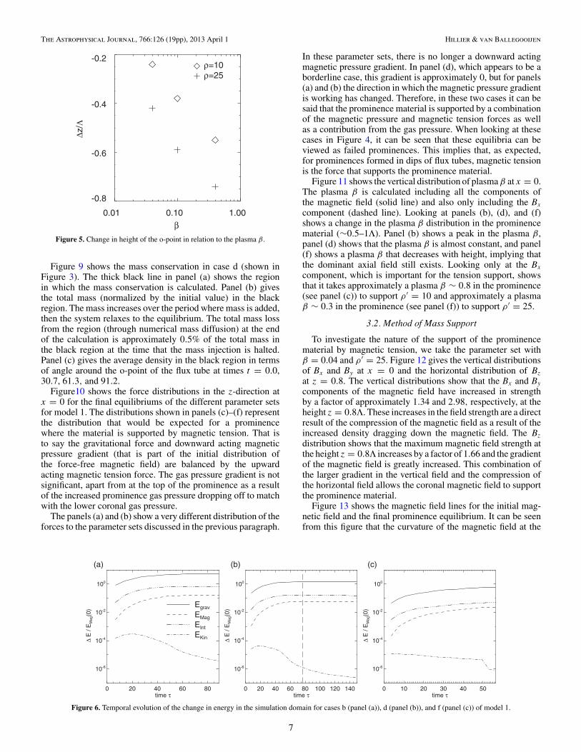
An expanded view of the prominence density distribution andthe magnetic field of the prominence is shown in Figure 4. Thisclearly shows the structure described previously. As with theglobal field, the field lines plotted in the figure that are furthestfrom the o-point do not change greatly, whereas those field linesthat are closer to the o-point undergo more stretching to supportthe prominence material. The compression of the magnetic fieldcan be seen. Case f, with the ρ ′ = 25 and β = 0.04, has astructure that represents that of the expected structure of thequiescent prominence that is supported by magnetic tension.The drop in o-point with height is given in Figure 5. The changein height from the original o-point is plotted against the plasmaβ. It can be seen that the change in height is strongly related tothe change in plasma β.

Figure 6 shows the evolution of the magnetic, kinetic, grav-itational potential, and internal energies with time for cases b,

5

The Astrophysical Journal, 766:126 (19pp), 2013 April 1 Hillier & van Ballegooijen

-1.0 -0.5 0.0 0.5 1.0X/Λ

0.0

0.5

1.0

1.5

2.0

2.5

Z/Λ

-1.0 -0.5 0.0 0.5 1.0X/Λ

0.0

0.5

1.0

1.5

2.0

2.5

Z/Λ

-1.0 -0.5 0.0 0.5 1.0X/Λ

0.0

0.5

1.0

1.5

2.0

2.5

Z/Λ

-1.0 -0.5 0.0 0.5 1.0X/Λ

0.0

0.5

1.0

1.5

2.0

2.5

Z/Λ

-1.0 -0.5 0.0 0.5 1.0X/Λ

0.0

0.5

1.0

1.5

2.0

2.5

Z/Λ

-1.0 -0.5 0.0 0.5 1.0X/Λ

0.0

0.5

1.0

1.5

2.0

2.5

Z/Λ

)b()a(

)d()c(

)f()e(

35.00

20.00

5.00

Figure 4. Local change in density distribution and magnetic field distribution (contours show magnetic vector potential) for model 1 in the six different cases lookingonly at the prominence region. Going from left to right shows the increase in mass added and from top to bottom shows the decrease in plasma β. The drop in theheight of the o-point and stretching of the magnetic field are clearly visible, especially for the high β cases.

(A color version of this figure is available in the online journal.)

d, and f. The plots in each simulation show the change in en-ergy from the initial state, with the values shown normalized bythe initial magnetic energy (IME) of the respective simulation.These figures show that after the mass has been added to theflux rope, the system relaxes with a steady decrease in total ki-netic energy (TKE) until the TKE/IME < 10−6 and the otherenergies have reached constant values. The vertical dashed linein panel (b) shows the approximate time at which the condi-tions for equilibrium are satisfied, with the continued evolutionshown for reference.

Next, the horizontal and vertical distributions of the hydro-dynamic variables are given. The horizontal distributions at z =0.8Λ are shown in Figure 7. For the models where a prominenceis supported by magnetic tension showing a thin, high density

prominence region, the horizontal pressure distribution showsthat the pressure at the center of the prominence has increasedby a factor of two when compared to the background pressure.

Figure 8 gives the vertical distributions of the hydrodynamicvariables at x = 0. The two extreme cases, which implytwo different mechanisms of support, are shown in panels (b)and (f). The density distributions shown are very different.The distribution shown in panel (b) decreases exponentially,implying that the material is supported by a pressure gradient(either gas or magnetic). The distribution shown in panel (f)has a density distribution that is almost constant with height inthe prominence, as well as a pressure distribution that is alsoalmost constant with height. In this case, the dense material issupported by magnetic tension.

6

The Astrophysical Journal, 766:126 (19pp), 2013 April 1 Hillier & van Ballegooijen

0.01 0.10 1.00β

-0.8

-0.6

-0.4

-0.2

Δz/Λ

ρ=10ρ=25

Figure 5. Change in height of the o-point in relation to the plasma β.

Figure 9 shows the mass conservation in case d (shown inFigure 3). The thick black line in panel (a) shows the regionin which the mass conservation is calculated. Panel (b) givesthe total mass (normalized by the initial value) in the blackregion. The mass increases over the period where mass is added,then the system relaxes to the equilibrium. The total mass lossfrom the region (through numerical mass diffusion) at the endof the calculation is approximately 0.5% of the total mass inthe black region at the time that the mass injection is halted.Panel (c) gives the average density in the black region in termsof angle around the o-point of the flux tube at times t = 0.0,30.7, 61.3, and 91.2.

Figure10 shows the force distributions in the z-direction atx = 0 for the final equilibriums of the different parameter setsfor model 1. The distributions shown in panels (c)–(f) representthe distribution that would be expected for a prominencewhere the material is supported by magnetic tension. That isto say the gravitational force and downward acting magneticpressure gradient (that is part of the initial distribution ofthe force-free magnetic field) are balanced by the upwardacting magnetic tension force. The gas pressure gradient is notsignificant, apart from at the top of the prominence as a resultof the increased prominence gas pressure dropping off to matchwith the lower coronal gas pressure.

The panels (a) and (b) show a very different distribution of theforces to the parameter sets discussed in the previous paragraph.

In these parameter sets, there is no longer a downward actingmagnetic pressure gradient. In panel (d), which appears to be aborderline case, this gradient is approximately 0, but for panels(a) and (b) the direction in which the magnetic pressure gradientis working has changed. Therefore, in these two cases it can besaid that the prominence material is supported by a combinationof the magnetic pressure and magnetic tension forces as wellas a contribution from the gas pressure. When looking at thesecases in Figure 4, it can be seen that these equilibria can beviewed as failed prominences. This implies that, as expected,for prominences formed in dips of flux tubes, magnetic tensionis the force that supports the prominence material.

Figure 11 shows the vertical distribution of plasma β at x = 0.The plasma β is calculated including all the components ofthe magnetic field (solid line) and also only including the Bxcomponent (dashed line). Looking at panels (b), (d), and (f)shows a change in the plasma β distribution in the prominencematerial (∼0.5–1Λ). Panel (b) shows a peak in the plasma β,panel (d) shows that the plasma β is almost constant, and panel(f) shows a plasma β that decreases with height, implying thatthe dominant axial field still exists. Looking only at the Bxcomponent, which is important for the tension support, showsthat it takes approximately a plasma β ∼ 0.8 in the prominence(see panel (c)) to support ρ ′ = 10 and approximately a plasmaβ ∼ 0.3 in the prominence (see panel (f)) to support ρ ′ = 25.

3.2. Method of Mass Support

To investigate the nature of the support of the prominencematerial by magnetic tension, we take the parameter set withβ = 0.04 and ρ ′ = 25. Figure 12 gives the vertical distributionsof Bx and By at x = 0 and the horizontal distribution of Bz

at z = 0.8. The vertical distributions show that the Bx and Bycomponents of the magnetic field have increased in strengthby a factor of approximately 1.34 and 2.98, respectively, at theheight z = 0.8Λ. These increases in the field strength are a directresult of the compression of the magnetic field as a result of theincreased density dragging down the magnetic field. The Bz

distribution shows that the maximum magnetic field strength atthe height z = 0.8Λ increases by a factor of 1.66 and the gradientof the magnetic field is greatly increased. This combination ofthe larger gradient in the vertical field and the compression ofthe horizontal field allows the coronal magnetic field to supportthe prominence material.

Figure 13 shows the magnetic field lines for the initial mag-netic field and the final prominence equilibrium. It can be seenfrom this figure that the curvature of the magnetic field at the

0 20 40 60 80time τ

10-6

10-4

10-2

100

Δ E

/ E

Mag

(0)

0 20 40 60 80 100 120 140time τ

10-6

10-4

10-2

100

Δ E

/ E

Mag

(0)

0 10 20 30 40 50time τ

10-6

10-4

10-2

100

Δ E

/ E

Mag

(0)

Egrav

EMag

EInt

EKin

(a) (b) (c)

Figure 6. Temporal evolution of the change in energy in the simulation domain for cases b (panel (a)), d (panel (b)), and f (panel (c)) of model 1.

7

The Astrophysical Journal, 766:126 (19pp), 2013 April 1 Hillier & van Ballegooijen

-2 -1 0 1 2X/Λ

0.1

1.0

10.0

Nor

mal

ized

qua

ntiti

es

-2 -1 0 1 2X/Λ

0.1

1.0

10.0

Nor

mal

ized

qua

ntiti

es-2 -1 0 1 2

X/Λ

0.1

1.0

10.0

Nor

mal

ized

qua

ntiti

es

-2 -1 0 1 2X/Λ

0.1

1.0

10.0

Nor

mal

ized

qua

ntiti

es

-2 -1 0 1 2X/Λ

0.1

1.0

10.0

Nor

mal

ized

qua

ntiti

es

-2 -1 0 1 2X/Λ

0.1

1.0

10.0

Nor

mal

ized

qua

ntiti

es

Pressureρ

Temperature )b()a(

)d()c(

)f()e(

Figure 7. Horizontal distribution of the hydrodynamic variables for the six different parameter sets for model 1. The distribution is taken at the height z = 0.8Λ.

base of the prominence is not significantly changed by the addi-tion of mass, but that the magnetic field lines have accumulated.The curvature of the magnetic field, however, increases withheight, which follows the decrease in the horizontal componentof the magnetic field. This implies that in our model the supportfor the prominence material happens in the following way.

1. The dense material falls due to gravity, pulling the magneticfield with it, stretching the magnetic field.

2. The stretched magnetic field exerts a tension force on thewhole of the flux tube, which then is pulled downward.

3. As the flux tube drops, the magnetic field in the prominencecompresses especially at the base of the prominence,meaning that a reduced curvature can produce a strongertension force.

4. This tension force, where the curvature of the magneticfield changes significantly with height, can now support theprominence.

3.3. Varying Mass Input Width

Here, we investigate the change in the prominence structurethat results from the change in the width over which mass isinput. The parameter set used to investigate this is β = 0.04and ρ ′ = 25. To look at the difference in width, the mass isadded with widths of Wp = 0.16Λ, 0.32Λ, and 0.48Λ used inEquation (14).

Figure 14 shows the global and local magnetic field anddensity distribution for, from top to bottom, widths of Wp =0.16Λ, 0.32Λ, and 0.48Λ. It can be seen that the mass inputwith greater width results in a lower o-point and a higher centraldensity. This higher density comes because, even though theo-point drops, this does not significantly change the curvatureof the magnetic field. As there is a component of gravity thatworks along the direction of the magnetic field, the prominencewill contract until the pressure gradient in the prominence isgreat enough to balance the gravitational force. Therefore, for

8

The Astrophysical Journal, 766:126 (19pp), 2013 April 1 Hillier & van Ballegooijen

0 1 2 3 4 5Z/Λ

10-1

100

101

102

103

104

105

Nor

mal

ized

qua

ntiti

es

0 1 2 3 4 5Z/Λ

10-1

100

101

102

103

104

105

Nor

mal

ized

qua

ntiti

es

0 1 2 3 4 5Z/Λ

10-1

100

101

102

103

104

105

Nor

mal

ized

qua

ntiti

es

0 1 2 3 4 5Z/Λ

10-1

100

101

102

103

104

105

Nor

mal

ized

qua

ntiti

es

0 1 2 3 4 5Z/Λ

10-1

100

101

102

103

104

105

Nor

mal

ized

qua

ntiti

es

0 1 2 3 4 5Z/Λ

10-1

100

101

102

103

104

105

Nor

mal

ized

qua

ntiti

es

Pressureρ

Temperature )b()a(

)d()c(

)f()e(

Figure 8. Vertical distribution of temperature, pressure, and density for the six parameter sets of model 1. The distributions are taken at the horizontal position x = 0Λ.

Figure 9. Figure showing the evolution of the total mass of a ring section of the flux rope. Panel (a) shows the flux tube with the prominence, with the thick blackline showing the region where the mass evolution is calculated. Panel (b) shows the evolution of mass with time. Panel (c) shows the density by position (as angle θ

around the o-point) at time t = 0.0, 30.7, 61.3, and 91.2.

(A color version of this figure is available in the online journal.)

9

The Astrophysical Journal, 766:126 (19pp), 2013 April 1 Hillier & van Ballegooijen

0 1 2 3 4 5Z/Λ

-40

-20

0

20

40

Nor

mal

ized

forc

e

0 1 2 3 4 5Z/Λ

-40

-20

0

20

40

Nor

mal

ized

forc

e

0 1 2 3 4 5Z/Λ

-40

-20

0

20

40

Nor

mal

ized

forc

e

0 1 2 3 4 5Z/Λ

-40

-20

0

20

40

Nor

mal

ized

forc

e

0 1 2 3 4 5Z/Λ

-40

-20

0

20

40

Nor

mal

ized

forc

e

0 1 2 3 4 5Z/Λ

-40

-20

0

20

40

Nor

mal

ized

forc

e

TensionGravity

Pressure GradientMag. Pressure Gradient

Total

)b()a(

)d()c(

)f()e(

Figure 10. Force distribution for the six different parameter sets for model 1. The distributions are taken at the horizontal position x = 0Λ.

greater widths for adding the prominence material, the finalprominence density becomes higher.

To analyze the width of the prominence and how it changeswith the input width, the prominence density, and pressuredistributions at the height z = 0.6Λ is fitted with a Gaussiandistribution and the FWHM of this fitted Gaussian distribution isthen taken as the width of the prominence. For the three models,the FWHMs of the fitted Gaussian distributions are 0.1Λ, 0.18Λ,and 0.26Λ for the density and 0.1Λ, 0.20Λ, and 0.26Λ for thepressure. Therefore, the width of the prominence can be seento have contracted by a factor of 1.5–2. This implies that, evenwith the drop in o-point height, which can reduce the curvatureof the magnetic field, the accretion of mass through contractionof the prominence along the direction of the magnetic field issufficient to pull in the prominence material.

Looking at the vertical force balance, see Figure 15, it is clearthat the input width of Wp = 0.48Λ is approaching being a failedprominence due to the larger support from pressure gradients.

Therefore, it is unlikely that β = 0.04 is sufficient to supportprominences with higher mass.

3.4. Investigation of More Complex Magnetic Field Model

Here, we will present the results from the mass addition for adifferent magnetic field model shown in Figure 1(b). This modelis called model 2. This model differs from the model used forthe previous results in three key areas:

1. The o-point is initially higher by approximately 0.5Λ.2. The ratio of By to Bx is ∼11.3. There is an x-point below the o-point.

With these differences, there is a significant change in how thesystem behaves. In fact, for the simulated parameters, the modeldoes not reach an equilibrium. It should be noted here that theplasma β values investigated here are β = 0.1, 0.04, and 0.01 togive a stronger Bx component of the magnetic field to increasethe ability of the field to support the plasma.

10

The Astrophysical Journal, 766:126 (19pp), 2013 April 1 Hillier & van Ballegooijen

0 1 2 3 4 5Z/Λ

0.1

1.0

10.0

Pla

sma

Bet

a

0 1 2 3 4 5Z/Λ

0.1

1.0

10.0

Pla

sma

Bet

a

0 1 2 3 4 5Z/Λ

0.01

0.10

1.00

10.00

Pla

sma

Bet

a

0 1 2 3 4 5Z/Λ

0.01

0.10

1.00

10.00

Pla

sma

Bet

a

0 1 2 3 4 5Z/Λ

0.01

0.10

1.00

10.00

Pla

sma

Bet

a

0 1 2 3 4 5Z/Λ

0.01

0.10

1.00

10.00

Pla

sma

Bet

a

)b()a(

)d()c(

)f()e(

Plasma beta for only Bx

Total plasma beta

Figure 11. Plasma β distribution with height for the six different parameter sets for model 1 taken at x = 0. The solid line shows the plasma β for all magnetic fieldcomponents, and the dashed line shows the plasma β for the Bx component, which is related to the amount of tension the magnetic field can exert.

0 1 2 3 4 5Z/Λ

-3

-2

-1

0

1

2

Bx

0 1 2 3 4 5Z/Λ

0

1

2

3

4

By

-2 -1 0 1 2X/Λ

-2

-1

0

1

2

Bz

InitialEquilibrium

(a) (b) (c)

Figure 12. Magnetic field distribution for model 1 parameter set f. The Bx and By distributions are taken at x = 0 and the Bz distribution is taken at z = 0.8Λ.

11

The Astrophysical Journal, 766:126 (19pp), 2013 April 1 Hillier & van Ballegooijen

-0.2-0.10.0 0.1 0.2X/Λ

0.6

0.8

1.0

1.2

1.4

Z/Λ

-0.2-0.10.0 0.1 0.2X/Λ

0.6

0.8

1.0

1.2

1.4

Z/Λ

(b)(a)

Figure 13. Magnetic field distribution of the parameter set β = 0.04 andρ′ = 25 both (a) before the mass addition and (b) once the magneto-hydrostaticequilibrium has formed. Lines show the distribution of Ay (x, z), where the samevalues of Ay (x, z) are used to draw the contours for each plot.

The reason for the significant change from the previous modelcan be seen in Figure 16 which shows the local distributionof the magnetic field and the density change. As with theprevious model, for the global field the overlying arcade remainsreasonably unchanged, but it can be seen in Figure 16 thata long, vertical current sheet develops in the prominencemagnetic field and with reconnection occurring at the x-point.The change in topology that this implies means that there isdissipation of the horizontal field component that is needed tosupport the prominence material. Therefore, while reconnectionis occurring it is not possible for the prominence material toform a steady state. It can also be seen that for the β = 0.1simulations, a long thin current that forms as the magnetic fieldis stretched by the falling plasma.

The temporal evolution of the energies for cases b(panel (a)), d (panel (b)), and f (panel (c)) is displayed inFigure 17. In all three cases, the maximum KE has not fallenbelow the set threshold and for case b it can be seen that theTKE is increasing as the simulation progresses. The reasonwhy the maximum KE does not fall below the set criteria ispresented in Figure 18, which shows the temporal evolution

-2 -1 0 1 2X/Λ

0

1

2

3

4

5

Z/Λ

-1.0 -0.5 0.0 0.5 1.0X/Λ

0.0

0.5

1.0

1.5

2.0

2.5

Z/Λ

-2 -1 0 1 2X/Λ

0

1

2

3

4

5

Z/Λ

-1.0 -0.5 0.0 0.5 1.0X/Λ

0.0

0.5

1.0

1.5

2.0

2.5

Z/Λ

-2 -1 0 1 2X/Λ

0

1

2

3

4

5

Z/Λ

-1.0 -0.5 0.0 0.5 1.0X/Λ

0.0

0.5

1.0

1.5

2.0

2.5

Z/Λ

)b()a(

)d()c(

)f()e(

45.00

30.00

15.00

Figure 14. Global and local change of the magnetic field and density distributions for the models with different input widths for the mass.

(A color version of this figure is available in the online journal.)

12

The Astrophysical Journal, 766:126 (19pp), 2013 April 1 Hillier & van Ballegooijen

Figure 15. Force distribution for the three different input widths for model 1. The distributions are taken at the horizontal position x = 0Λ.

-1.0 -0.5 0.0 0.5 1.0X/Λ

0.0

0.5

1.0

1.5

2.0

2.5

Z/Λ

-1.0 -0.5 0.0 0.5 1.0X/Λ

0.0

0.5

1.0

1.5

2.0

2.5

Z/Λ

-1.0 -0.5 0.0 0.5 1.0X/Λ

0.0

0.5

1.0

1.5

2.0

2.5

Z/Λ

-1.0 -0.5 0.0 0.5 1.0X/Λ

0.0

0.5

1.0

1.5

2.0

2.5

Z/Λ

-1.0 -0.5 0.0 0.5 1.0X/Λ

0.0

0.5

1.0

1.5

2.0

2.5

Z/Λ

-1.0 -0.5 0.0 0.5 1.0X/Λ

0.0

0.5

1.0

1.5

2.0

2.5

Z/Λ

)b()a(

)d()c(

)f()e(

25.00

15.00

5.00

Figure 16. Local change of the magnetic field and density distributions for model 2.

(A color version of this figure is available in the online journal.)

of the vertical velocity at x = 0 for case f. Peaks in the ve-locity can be found at the position of the x-point, highlight-ing this region’s importance for the continued evolution of thesystem.

The relation between the drop in the o-point and howdistended the magnetic field becomes for this model is verydifferent from the previous model. This is because, as mentionedpreviously, a long, vertical current sheet develops above the

13

The Astrophysical Journal, 766:126 (19pp), 2013 April 1 Hillier & van Ballegooijen

0 50 100 150 200time τ

10-7

10-6

10-5

10-4

10-3

10-2

10-1

100

Δ E

/ E

Mag

(0)

0 20 40 60 80 100 120 140time τ

10-7

10-6

10-5

10-4

10-3

10-2

10-1

Δ E

/ E

Mag

(0)

0 20 40 60 80 100 120 140time τ

10-7

10-6

10-5

10-4

10-3

10-2

10-1

Δ E

/ E

Mag

(0)

Egrav

EMag

EInt

EKin

(a) (b) (c)

Figure 17. Temporal evolution of the change in energy in the simulation domain for cases b (panel (a)), d (panel (b)), and f (panel (c)) of model 2.

0 1 2 3 4 5Z/Λ

-0.005

0.000

0.005

0.010

0.015

0.020

W/C

s

t=126τt=158τt=93τ

t=190τ

Figure 18. Temporal evolution of the vertical velocity (w) at x = 0Λ. Thishighlights that even though the velocities in the prominence are small, a sharpjump in velocity (showing a converging flow) exists at the x-point.

prominence where only a small component of the horizontalfield remains. Where, in the previous case, the o-point would fallwith the material, here the o-point is stretched into a line wherethere is no Bx component of the magnetic field (this is discussedlater). In this respect, it can be seen that the movement of theo-point is determined by the amount of tension that is neededby the magnetic field to support the mass and the strength of themagnetic pressure at the o-point. The change in the height ofthe o-point is shown in Figure 19.

The vertical distribution (at x = 0Λ) is shown in Figure 20.This shows, apart from panel (e), similar distributions ofthe prominence density to the failed prominences shown inSection 3.1. Only in panel (e) does the dense material appearto be supported to some extent by magnetic tension. This is notsurprising given the significantly weaker horizontal magneticfield distribution.

Another point of note is the drop of density between theprominence and the region below. This is a result of the x-point,which creates a thin region with coronal density beneath theprominence; this can be seen in Figure 16. This region maybe unstable to the magnetic Rayleigh–Taylor instability, asobserved in prominences by Berger et al. (2008, 2010) andstudied numerically by Hillier et al. (2012a, 2011a).

It should be noted again that this model does not reach anequilibrium. This can be seen by the vertical forces in theprominence, shown in Figure 21, that shows a small net forcein the prominence that peaks around the position of the x-point.

0.001 0.010 0.100 1.000β

-1.0

-0.8

-0.6

-0.4

-0.2

Δ z/Λ

ρ=10ρ=25

Figure 19. Change in o-point height for model 2. This also includes results fromthe case where β = 0.4.

The main difference between this model and the previous modelshown in Section 3.1 is that the main upward oriented force inthe prominence region is gas pressure; this is especially clearin panel b of Figure 21. Therefore, these prominences are onlyusing the magnetic field to collimate the material and are usinggas pressure to support the material. This implies that the fieldstrength of the horizontal field is not sufficient and so lowerplasma β values are necessary for this 2.5D model. For theβ = 0.01 case the force distributions are beginning to approachthose of the tension support models, i.e., panel f of Figure 9, butclearly smaller β values are necessary for tension support to bepossible.

Figure 22 shows the plasma β for this model. Again both theplasma β calculated using all the magnetic field components(solid line) and only the Bx component are shown. Though theplasma β values are very small, looking at the Bx componentshows that the horizontal field is not strong enough to support thematerial through magnetic tension. Only in the case presented inpanel (e) has the horizontal field become close to strong enoughto support the added mass.

Figure 23 gives the vertical distributions of the Bx and Bycomponents of the magnetic field at x = 0 and the horizontaldistribution of Bz at z = 1Λ. The distribution of Bx (panel (a))shows, as mentioned previously, that the o-point is no longera point, but a vertical line with little or no Bx component ofthe magnetic field. As is known from the studies of the tearinginstability (Furth et al. 1963), when this line reaches a criticallength, the system is unstable to the formation of magnetic

14

The Astrophysical Journal, 766:126 (19pp), 2013 April 1 Hillier & van Ballegooijen

0 1 2 3 4 5Z/Λ

10-1

100

101

102

103

104

105

Nor

mal

ized

qua

ntiti

es0 1 2 3 4 5

Z/Λ

10-1

100

101

102

103

104

105

Nor

mal

ized

qua

ntiti

es

0 1 2 3 4 5Z/Λ

10-1

100

101

102

103

104

105

Nor

mal

ized

qua

ntiti

es

0 1 2 3 4 5Z/Λ

10-1

100

101

102

103

104

105

Nor

mal

ized

qua

ntiti

es

0 1 2 3 4 5Z/Λ

10-1

100

101

102

103

104

105

Nor

mal

ized

qua

ntiti

es

0 1 2 3 4 5Z/Λ

10-1

100

101

102

103

104

105

Nor

mal

ized

qua

ntiti

es

Pressureρ

Temperature )b()a(

)d()c(

)f()e(

Figure 20. Vertical distribution of the hydrodynamic variables for model 2. The distributions are taken at the horizontal position x = 0Λ.

islands. The distribution of Bz which results in the currentsheet in this |Bx | 1 region is shown in panel (c). This willresult in reconnection which separates the prominence magneticfield into a separate flux tube embedded in the initial coronalflux tube. Above the prominence region, the By distribution ofthe magnetic field does not show any significant change, butthere is an accumulation of the axial field at the base of theprominence.

Comparing the results from this case with the results fromcase 1, it is clear that there is a difference in the way the magneticfield evolves toward a magneto-hydrostatic equilibrium. Forthe case presented in this subsection, the o-point is stretchedresulting in the bottom of this region giving the large drop inthe o-point in some cases shown in Figure 19; this stretchingof the o-point into a line over which there is little to no Bxcomponent of the magnetic field, especially for the parametercase b as this has a weaker magnetic field, gives a long, thincurrent sheet. The step-like current sheet can be clearly seen forthe Bz distribution in this parameter set. For parameter set f,where the magnetic field is stronger, this is not so pronounced,but the weak horizontal field is still noticeable. This stretching ofthe o-point results from a divergence of the velocity field in thez-direction, which has its peak at the o-point. This divergencewould advect the horizontal field away from the o-point, creatinga long, thin region where the horizontal field is either 0 or closeto zero (see Figure 23, panel (a)).

For model 1, two different support mechanisms were found:pressure support and tension support. For model 2 neither isfound to be effective. The tension support would not be ableto work because the horizontal field is insufficiently strong tosupport the magnetic field through magnetic tension. Thereis, however, a very large By component, especially in theβ = 0.01 model, so it could be expected that pressure supportmay be possible. This mechanism does not work in this modelbecause of the reconnection at the x-point, which means thatplasma trapped inside dips and supported by magnetic pressurecan escape from the system. Figure 24 shows the change in themass in the flux tube (normalized so the initial mass is 1). Asreconnection is occurring, it should be noted that the size ofthe flux tube is decreasing in time. From the peak in the mass,28% of the mass is lost over a time of ∼100τ ; over the sameperiod only a maximum of 2% of the total mass loss can beattributed to cross-field diffusion of mass out of the flux ropedue to numerical diffusion. Therefore, the reconnection allowsthe mass to escape the prominence.

4. SUMMARY AND DISCUSSION

In this study, we have looked at the support of mass againstgravity by the Lorentz force of a coronal flux rope. It was foundthat for the case where the support of the mass has a largecontribution from pressure gradients, the structure of the formed

15

The Astrophysical Journal, 766:126 (19pp), 2013 April 1 Hillier & van Ballegooijen

Figure 21. Force distribution for the six different parameter sets for model 2. The distributions are taken at the horizontal position x = 0Λ.

prominence was very different from observed prominences,therefore this case can be seen as a failed prominence. However,when magnetic tension is the main force for the support of thedense material, then a prominence-like structure is formed.

The mechanism for the tension support results from two keyprocesses. The upper region of the prominence is supportedby the stretching of the magnetic field, which results in highertension. However, at the base of the prominence, the supportcomes from the curvature of compressed magnetic field. As themagnetic field is compressed, it does not need a strong radius ofcurvature to produce the same tension as the magnetic field at thetop of the prominence. The compression of the magnetic field isa direct result of the added mass, which pulls down the o-pointso magnetic field accumulates at the base of the prominence.

Comparison between the two models showed that the drop inthe o-point, and how much the magnetic field was stretched,depended heavily on the ratio of the axial field (By) to thehorizontal field (Bx). It appears that when this ratio is large,the height of the o-point becomes more stable and there is

greater stretching of the magnetic field, whereas when the ratiois small then there is a greater drop in the o-point height withless stretching of the magnetic field. However, due to the weakhorizontal field and, in some part, to numerical reconnectionin these models (both at the x-point and in the prominencecurrent sheet), it has not been possible to achieve the magneto-hydrostatic equilibrium for the second model, therefore it isdifficult to give these results with greater accuracy.

The reconnection found in model 2 was a result of the nu-merical dissipation of the magnetic field. Therefore, it can beexpected that the use of more grid points, or a numerical schemethat is less dissipative, would slow down the rate of the recon-nection. Assuming Sweet–Parker reconnection, where the re-connection rate is given by vin/vAS−1/2 with vin as the inflowvelocity, vA as the Alfven velocity, and S as the Lundquist num-ber, reduction in the numerical diffusion will slow down therate at which magnetic field reconnects. However, only in thetheoretical limit of 0 error can it be expected that numerical re-connection would not occur allowing a true equilibrium to form.

16

The Astrophysical Journal, 766:126 (19pp), 2013 April 1 Hillier & van Ballegooijen

0 1 2 3 4 5Z/Λ

0.01

0.10

1.00

10.00

Pla

sma

Bet

a

0 1 2 3 4 5Z/Λ

0.01

0.10

1.00

10.00

Pla

sma

Bet

a0 1 2 3 4 5

Z/Λ

0.001

0.010

0.100

1.000

10.000

Pla

sma

Bet

a

0 1 2 3 4 5Z/Λ

0.001

0.010

0.100

1.000

10.000

Pla

sma

Bet

a

0 1 2 3 4 5Z/Λ

0.001

0.010

0.100

1.000

10.000

Pla

sma

Bet

a

0 1 2 3 4 5Z/Λ

0.001

0.010

0.100

1.000

10.000

Pla

sma

Bet

a

)b()a(

)d()c(

)f()e(

Figure 22. Vertical distribution of plasma β for model 2. The solid line shows the plasma β for all magnetic field components, and the dashed line shows the plasmaβ for the Bx component, which is related to the amount of tension the magnetic field can exert.

Looking at the plasma β as shown in Figure 11, only whenthe plasma β of the magnetic field supporting the dense materialis less than 0.3 is it possible to support the prominence materialin the ρ ′ = 25 case. If we extrapolate to greater prominencedensities, then for support of the material to be possible, it wouldbe necessary that plasma β < 0.1. For a prominence with gaspressure of p = 0.3 dyn, the required magnetic field strengthwould be B >

√p8π/0.1 ∼ 8 G, which is consistent with

the average polar crown prominence magnetic field strengthof ∼5 G (Anzer & Heinzel 2007). The relationship betweenthe magnetic field strength and the drop in the height of the fluxtube o-point was theoretically analyzed by Blokland & Keppens(2011a), given in Equation (25) of that paper. However, applyingthis equation to the results of model 1, it was found that thedrop in o-point was grossly overestimated for β = 0.4 andunderestimated for β = 0.04. Therefore, the assumption thatgravity can be studied as a small perturbation to the system,as used in Blokland & Keppens (2011a), does not apply to theprominences studied in this work.

The mass support we study is 2.5D, therefore the tensionterm By∂Bz/∂y cannot be invoked to help support the material.For model 2, it was not possible to support the dense materialdue to the large ratio of axial field to horizontal field, withBy/Bx ∼ 11. If variations along the axis of the prominencewere allowed, then this axial field could be used for the support.Therefore, it should be expected that in three dimensions,support of material should be possible for plasma β that arecloser to unity than the values found in this study. This wouldcancel out the factor of four reduction in prominence densityfor the prominences studied here. It would be an interestingresearch topic to extend these simulations to three dimensions.It would also be interesting to then extend this work to includeCowling resistivity (Braginskii 1965; Cowling 1957), as it hasbeen shown to alter the prominence magnetic field over thetimescale of the Cowling resistivity (Hillier et al. 2010).

In this paper, a 2.5D model for a prominence is considered.Therefore, the prominence flux rope is not tied to the photo-sphere at its ends, and will always be unstable to internal kink

17

The Astrophysical Journal, 766:126 (19pp), 2013 April 1 Hillier & van Ballegooijen

0 1 2 3 4 5Z/Λ

-1.0

-0.5

0.0

0.5

1.0

1.5

2.0

Bx

0 1 2 3 4 5Z/Λ

0.0

0.5

1.0

1.5

2.0

2.5

By

-2 -1 0 1 2X/Λ

-1.5

-1.0

-0.5

0.0

0.5

1.0

1.5

Bz

InitialFinal

)c()b()a(

0 1 2 3 4 5Z/Λ

-2

0

2

4

6

Bx

0 1 2 3 4 5Z/Λ

0

1

2

3

4

5

6

By

-2 -1 0 1 2X/Λ

-4

-2

0

2

4

Bz

InitialFinal

)f()e()d(

Figure 23. Distribution of the individual components of the magnetic field for model 2 parameter set b (top row) and parameter set f (bottom row). The Bx and Bydistributions are taken at x = 0 and the Bz distribution is taken at z = 1Λ.

0 50 100 150t/τ

0

2

4

6

8

tota

l[ρ]/t

otal

[ρ(t

=0)

]

Figure 24. Temporal evolution of normalized mass in the flux tube for case fof model 2. This figure highlights the drain in mass from the flux tube due toreconnection at the x-point.

modes. Real-world prominences have finite length, and kink in-stabilities can be suppressed by line-tying effects. To gauge thestability of the systems considered here, let us assume thatthe modeled flux ropes have a length Ly = 10Λ ≈ 550 Mm.The stability depends on the so-called safety factor, which isdefined by q(A) = B(A)/Ly

∮ds/|∇⊥A|, where the integral

is over a closed contour A(x, z) = constant. We find that formodel 1 the safety factor increases from about 0.15 at the outeredge of the flux rope to 0.28 on its axis, while for model 2 thesafety factor is much larger and nearly constant, q ≈ 2.4. Kinkinstability is predicted to occur when q < 1, so model 1 is likelyto be unstable, but model 2 is stable.

The parameters for model 1 were chosen to make the heightof the flux rope axis as large as possible and comparable tothe height of observed prominences, zaxis ≈ 1.5Λ ≈ 83 Mm,because the axis determines the height of the dips. We found thatthis observational constraint can be satisfied only for relativelyhigh values of the total current Jy. This leads to highly twistedfields that tend to be kink unstable. We do not believe thatreal prominences are necessarily so highly twisted. However,with the present size of the computational domain and usingEquations (4) and (6) we were unable to obtain a weakly twistedflux rope with its axis at sufficiently large height. The issueof kink instability is not so important for the present workbecause we are mainly interested in the magnetic support ofthe prominence plasma. However, in future modeling otherexpressions for the photospheric flux distribution A(x, 0) and/or the axial field B(A) should be explored.

Blokland & Keppens (2011b) presented the condition for theonset of the continuum convective instability in prominences.A sufficient condition for the stability of the system is if theBrunt–Vaisala frequency projected onto a flux surface,

N2BV,pol = −

[Bθ · ∇p

ρB

] [Bθ · ∇S

ρBS

], (15)

is greater than or equal to 0 (N2BV,pol � 0) throughout the

plasma. The models investigated in this paper do not satisfythis condition, with the frequency in the dense prominencematerial N2

BV,pol = 0 but N2BV,pol < 0 in the regions where the

density transitions from the high prominence density to the lowcoronal density. As the models studied here relax to 2.5D MHDequilibria, we know that the systems under study are likely to

18

The Astrophysical Journal, 766:126 (19pp), 2013 April 1 Hillier & van Ballegooijen

be stable to ky = 0 modes of this instability. However, it is stillpossible that the instability could grow for ky �= 0 modes.

As investigated in Figure 8 of Blokland & Keppens (2011b),with larger density or weaker magnetic field, gravitationaleffects modify the growth rate of the continuum convectiveinstability. Therefore, this instability could be occurring inobserved prominences resulting in the flows of the prominencematerial that have been observed (e.g., Kubota & Uesugi 1986;Chae 2010). It would be very interesting to investigate thisinstability in terms of the conditions for its onset and thenonlinear evolution of the instability in a prominence geometryas this may provide a different explanation to the other modelsin the literature so far based on reconnection (e.g., Petrie &Low 2005; Chae 2010; Hillier et al. 2012b) or condensationformation (e.g., Haerendel & Berger 2011; Low et al. 2012a,2012b).

It must be noted that the free energy of the magnetic fieldsstudied here is rather high, a few times larger than the energyof the potential magnetic field. It has been shown that coronalmagnetic fields with such large free energies would erupt (Mooreet al. 2012). Here, we keep the magnetic field pinned down byusing a symmetric boundary at the top of the calculation domain,which allows a stable force-free field to form. In terms of thestudy presented here, where the formation of a prominence inmagnetic dips is studied, it does not present a large problem,but it may be difficult to apply these models to analyze theglobal stability of the system. It should be noted that Su & vanBallegooijen (2012) developed a global NLFFF model of anobserved quiescent prominence and found that the model fluxrope was stable but close to the limit of stability. Therefore, itappears to be possible to construct stable magnetic equilibria ofthe type studied in this paper. Extending the method presentedin this paper to study prominences where the magnetic fieldis based on observed photospheric magnetic field would be aninteresting research topic.

The authors thank the staff and students of Kwasan and Hidaobservatories for their support and comments. The authors thankthe referee for comments and suggestions that helped to improvethe presentation of this work. This work was supported in partby the Grant-in-Aid for the Global COE program “The NextGeneration of Physics, Spun from Universality and Emergence”from the Ministry of Education, Culture, Sports, Science andTechnology (MEXT) of Japan. This work was supported bythe Hinode/XRT project under NASA grant NNM07AB07C.Hinode is a Japanese mission developed and launched by ISAS/JAXA, with NAOJ as domestic partner and NASA and STFC(UK) as international partners. It is operated by these agenciesin cooperation with ESA and the NSC (Norway). The MHDrelaxations presented in this paper were carried out on theSIMSV cluster at Kwasan observatory.

REFERENCES

Aly, J.-J. 2011, ApJ, 746, 52Anzer, U. 1969, SoPh, 8, 37Anzer, U., & Heinzel, P. 2007, A&A, 467, 1285Aulanier, G., & Demoulin, P. 2003, A&A, 402, 769Aulanier, G., Demoulin, P., van Driel-Gesztelyi, L., Mein, P., & Deforest, C.

1998, A&A, 335, 309Berger, T. E., Shine, R. A., Slater, G. L., et al. 2008, ApJL,

676, L89Berger, T. E., Slater, G., Hurlburt, N., et al. 2010, ApJ, 716, 1288Blokland, J. W. S., & Keppens, R. 2011a, A&A, 532, A93Blokland, J. W. S., & Keppens, R. 2011b, A&A, 532, A94Braginskii, S. I. 1965, RvPP, 1, 205Chae, J. 2010, ApJ, 714, 618Cowling, T. G. 1957, Magnetohydrodynamics, Monographs on Astronomical

Subjects (New York: Interscience)de Toma, G., Casini, R., Burkepile, J. T., & Low, B. C. 2008, ApJL,

687, L123Dudık, J., Aulanier, G., Schmieder, B., Bommier, V., & Roudier, T. 2008, SoPh,

248, 29Engvold, O. 1981, SoPh, 70, 315Furth, H. P., Killeen, J., & Rosenbluth, M. N. 1963, PhFl, 6, 459Galindo-Trejo, J., & Schindler, K. 1984, ApJ, 277, 422Gibson, S. E., Foster, D., Burkepile, J., de Toma, G., & Stanger, A. 2006, ApJ,

641, 590Haerendel, G., & Berger, T. 2011, ApJ, 731, 82Hillier, A., Berger, T., Isobe, H., & Shibata, K. 2012a, ApJ, 746, 120Hillier, A., Isobe, H., Shibata, K., & Berger, T. 2011a, ApJL, 736, L1Hillier, A., Isobe, H., Shibata, K., & Berger, T. 2012b, ApJ, 756, 110Hillier, A., Isobe, H., & Watanabe, H. 2011b, PASJ, 63, L19Hillier, A., Shibata, K., & Isobe, H. 2010, PASJ, 62, 1231Hirayama, T. 1986, NASA Conference Publication, 2442, 149Hood, A. W., & Anzer, U. 1990, SoPh, 126, 117Kippenhahn, R., & Schluter, A. 1957, ZA, 43, 36Kubota, J., & Uesugi, A. 1986, PASJ, 38, 903Kuperus, M., & Raadu, M. A. 1974, A&A, 31, 189Labrosse, N., Heinzel, P., Vial, J.-C., et al. 2010, SSRv, 151, 243Leroy, J. L. 1989, in Proc. Workshop, Dynamics and Structure of Quiescent

Solar Prominences, Vol. 150, ed. E. R. Priest (Dordrecht: Kluwer), 77Liggett, M., & Zirin, H. 1984, SoPh, 91, 259Low, B. C., Berger, T., Casini, R., & Liu, W. 2012a, ApJ, 755, 34Low, B. C., & Hundhausen, J. R. 1995, ApJ, 443, 818Low, B. C., Liu, W., Berger, T., & Casini, R. 2012b, ApJ, 757, 21Luna, M., Karpen, J. T., & DeVore, C. R. 2012, ApJ, 746, 30Mackay, D. H., Karpen, J. T., Ballester, J. L., Schmieder, B., & Aulanier, G.

2010, SSRv, 151, 333Moore, R. L., Falconer, D. A., & Sterling, A. C. 2012, ApJ, 750, 24Petrie, G. J. D., Blokland, J. W. S., & Keppens, R. 2007, ApJ, 665, 830Petrie, G. J. D., & Low, B. C. 2005, ApJS, 159, 288Pneuman, G. W. 1983, SoPh, 88, 219Priest, E. R., Hood, A. W., & Anzer, U. 1989, ApJ, 344, 1010Rust, D. M., & Kumar, A. 1994, SoPh, 155, 69Stellmacher, G., & Wiehr, E. 1973, A&A, 24, 321Su, Y., & van Ballegooijen, A. 2012, ApJ, 757, 168Tandberg-Hanssen, E. 1995, Astrophysics and Space Science Library, Vol. 199

(Dordrecht: Kluwer)Ugai, M. 2008, PhPl, 15, 082306van Ballegooijen, A. A., & Cranmer, S. R. 2010, ApJ, 711, 164Xia, C., Chen, P. F., & Keppens, R. 2012, ApJL, 748, L26Xia, C., Chen, P. F., Keppens, R., & van Marle, A. J. 2011, ApJ, 737, 27Zweibel, E. G. 1982, ApJL, 258, L53

19