Embed Size (px)
Citation preview

On the Shortest Path Problemwith Pair Constraints
Master’s thesis
by
Michael Bruckner
Michael BrucknerMatrikelnr.: 4366915Ringstraße 1614979 Groß[email protected]
Submission date:February 25th 2015
Referees:Prof. Dr. Ralf Borndorfer
Dr. Nam Dung Hoang


Abstract
This thesis investigates the shortest path problem with pair constraints or the pairconstraint problem (PCP) for short. We consider two types of pair constraints,namely forbidden pairs and binding pairs consisting of two distinct vertices each.A path respects a forbidden pair if it uses at most one of the two vertices and itrespects a binding pair (x, y) if it uses also y, if x is used.
Within this thesis, we bring together and compare several formulations andvariants of the pair constraint problem and their complexities. We also col-lect existing recursive algorithms and present their running times. Most of thepresented contributions only consider forbidden pairs. We introduce a new recur-sive algorithm also handling binding pairs and prove its theoretical complexityof O(n4). We implemented the algorithm and tested it on real-world instancesprovided by Lufthansa Systems AG. Therefore we needed to develop a heuristictranslating the real-world data into an instance of the shortest path problem withpair constraints. This heuristic is presented as well as all computational results.
In Chapter 4, we start investigating the associated polytope of an integer pro-gram formulation of the shortest path problem with pair constraints. For thecase of one forbidden or binding pair, we find a complete linear description of theassociated polytope. We prove that the number of facets grows exponentially in|V | even in these simple cases. However, separation is still possible in polynomialtime. The complete linear description can be extended to the case of contiguouslydisjoint pairs.


Eigenstandigkeitserklarung
Hiermit erklare ich, nachstehende Masterarbeit eigenstandig und ohne Hilfe Drit-ter angefertigt zu haben. Alle Ubernahmen aus der Literatur sind als solchegekennzeichnet und im Literaturverzeichnis auf Seite 74 aufgelistet.
Hereby I confirm that I developed the following Master’s thesis entirely on myown without help of third parties. All adoptions from the literature are taggedas such and listed in the references section on Page 74.
Berlin, February 25, 2015
Michael Bruckner
Acknowledgements
This thesis arose from the project Flight Trajectory Optimization on AirwayNetworks at the Zuse-Institute Berlin, where I worked as a student researcher. Iwould like to express my gratitude to the project team, namely Prof. Dr. RalfBorndorfer, Marco Blanco, Dr. Nam Dung Hoang and Dr. Thomas Schlechte.They offered me the opportunity to work in their team and supervised me duringmy research and writing of this thesis. I want to emphasize the helpful assistanceof Marco, who essentially promoted many of the results presented in this workand was always available for all the time-consuming problems and questions. Ialso want to thank my family and friends, who supported me writing this thesis.
Thanks to the Federal Ministry of Education and Research in Germany andthe Lufthansa Systems AG, who supported this thesis.
v


Contents
1 Introduction 11.1 Motivation . . . . . . . . . . . . . . . . . . . . . . . . . . . . . . . 11.2 Literature Survey . . . . . . . . . . . . . . . . . . . . . . . . . . . . 31.3 Outline . . . . . . . . . . . . . . . . . . . . . . . . . . . . . . . . . 5
2 The Shortest Path Problem with Pair Constraints (PCP) 72.1 Preliminaries . . . . . . . . . . . . . . . . . . . . . . . . . . . . . . 72.2 Problem Statement . . . . . . . . . . . . . . . . . . . . . . . . . . . 11
2.2.1 Complexity . . . . . . . . . . . . . . . . . . . . . . . . . . . 142.2.2 Problem Variants . . . . . . . . . . . . . . . . . . . . . . . . 212.2.3 Structural Conditions . . . . . . . . . . . . . . . . . . . . . 23
3 Recursive Algorithms for the PCP 293.1 Existing Algorithms for PAFP . . . . . . . . . . . . . . . . . . . . 29
3.1.1 A Dynamic Programming Approach by Kovac . . . . . . . 293.1.2 Graph Contraction by Kolman and Pangrac . . . . . . . . . 323.1.3 A Contraction Variant for Arcs by Tan . . . . . . . . . . . 33
3.2 The Pair Constraint Reduction Algorithm . . . . . . . . . . . . . . 35
4 A Polyhedral Study of the PCP 394.1 A Complete Description for one Pair . . . . . . . . . . . . . . . . . 39
4.1.1 One Forbidden Pair . . . . . . . . . . . . . . . . . . . . . . 394.1.2 One Binding Pair . . . . . . . . . . . . . . . . . . . . . . . . 434.1.3 Separation and the Number of Facets . . . . . . . . . . . . 45
4.2 Contiguously Disjoint Pair Constraints . . . . . . . . . . . . . . . . 54
5 Computational Results 575.1 Implementation . . . . . . . . . . . . . . . . . . . . . . . . . . . . . 575.2 Extension to Obligatory Pairs . . . . . . . . . . . . . . . . . . . . . 585.3 A Translation Heuristic for Traffic Flow Restrictions . . . . . . . . 595.4 Test Instances . . . . . . . . . . . . . . . . . . . . . . . . . . . . . . 625.5 Results . . . . . . . . . . . . . . . . . . . . . . . . . . . . . . . . . . 63
6 Concluding Remarks 67
7 Appendix 697.1 Running Time Tables . . . . . . . . . . . . . . . . . . . . . . . . . 69
vii

Contents
7.2 List of Figures . . . . . . . . . . . . . . . . . . . . . . . . . . . . . 727.3 List of Tables . . . . . . . . . . . . . . . . . . . . . . . . . . . . . . 737.4 List of Algorithms . . . . . . . . . . . . . . . . . . . . . . . . . . . 737.5 References . . . . . . . . . . . . . . . . . . . . . . . . . . . . . . . . 74
viii

1 Introduction
1.1 Motivation
Air traffic is one of the most important means of transport, especially in Europe.There are over 120.000 commercial flights a month only in Germany [7], which ismore than 4.000 a day. Moreover, the air traffic increases every year by around5% [1]. Air traffic is connected with very high costs such as fuel, personnel orfees e.g. for overflying a country.
Before the year 2000, flight planning was very static. This means, for examplein Germany there were fixed routes for every pair of airports that could be lookedup in a document containing the standard routes. Beginning around the year2000, the philosophy came up that every trajectory is allowed. Since many airlinestended to optimize their flight routes, there were regions of very high trafficdensity. This was quite hard to handle for all the airlines and especially theagencies managing, regulating and controlling the air traffic. The solution wasto distribute the traffic over the sky and to separate different traffic flows basedon their direction, height or speed.
Mainly over Europe, this is achieved by settling a bunch of rules and restrictionsto be respected during planning of the flight routes. The rules base on manydifferent aspects of a flight, such as its departure or arrival, daytime, the season,the flight height or the usage of a concrete airspace or waypoint. Once a month,the European air traffic regulating organisation Eurocontrol publishes the so-called Route Availability Document (RAD) [11] of around 700 pages containingonly these rules. Figure 1.1 shows how the page number of the RAD has grownin recent years.
Most of the current flight trajectory optimization software was developed be-fore these rules are made. At this time, there were only a very few rules, whichthen could be involved manually or by simple methods. During the last years, thenumber of restrictions grew essentially to over 10.000. Whereas the previouslymentioned rules are a good way distributing the air traffic over the sky, math-ematically, they are very hard to involve in the optimization process of flighttrajectories. It is already a hard problem to find just any route respecting allrules not to mention computing the optimal one. For this reason, computing themost cost-efficient flight trajectory is a mathematical problem of great intererest.
The project “Flight Trajectory Optimization on Airway Networks” is a researchproject funded by the Federal Ministry of Education and Research in collabora-tion with the Lufthansa Systems AG. It focuses on developing algorithms that
1

1 Introduction
Figure 1.1: Average number of pages in the RAD per year. Source: LufthansaSystems AG
compute optimal flight trajectories for passenger or cargo airplanes through anairway network, which is a discrete and finite graph spanned over the wholeworld. It contains around 90,000 points and around 400,000 directed connectionsbetween the points.
The project belongs to the joint project “E-Motion – energy-efficient mobility”.In contrast to the computations in this airway network graph, another sub-projectof E-Motion is located for instance at the Helmut-Schmidt-University in Ham-burg. It is concerned with the same route optimization, but instead of a discretegraph, it deals with free flight. Whereas the airway network optimization is re-stricted to this network, free flight means that only origin and destination of theroute are given; every trajectory connecting these two is allowed. The free flightsystem is used mostly over the oceans, whereas the restriction to the graph isusually used over mainland.
The optimal trajectory in both optimization ways is highly depending on sev-eral factors such as the weather conditions. Since there is no connection to theground, airplane motion is not measured relatively to the ground, but to thesurrounding air. Thus, wind has an essential effect on the actual “length” of atrajectory and hence on its costs. A similar influence holds for instance for thetemperature and pressure of the air, but also for many other conditions. Be-side weather conditions, there are many governmental restrictions influencing theprice of flight trajectories as well. There are overflight fees for most countries,which have to be respected. These fees are calculated by different methods andnot all of them are computationally easy to include in the complete optimizationmethod.
Also relevant for the optimization of the trajectory are properties of the air-
2

1.2 Literature Survey
craft itself, for instance the initial weight, the airplane type or the speed mode.The performance of aircrafts is given as tables determining how fast an airplanerises or how much fuel it uses depending on the mentioned weather conditionsand its current weight. The conversion of these tables into usable data for theoptimization algorithm is a non trivial mathematical problem for itself, see [25].
This thesis is concerned with the rules of the RAD document. These rules areof various formats and types and parsing them is highly not trivial. This is whywe decided to focus on two particular cases, called forbidden pair constraints andbinding pair constraints. Together, they are called pair constraints and they arethe main mathematical concept of this thesis.
The problem of this thesis is the shortest path problem with pair constraints.We are given a directed graph D = (V,A), a source node s ∈ V , a destinationnode t ∈ V and two sets F ⊆ V × V and B ⊆ V × V of forbidden and bindingpairs, respectively. The problem is to find the shortest path P through thegraph connecting s and t and respecting all pair constraints. A forbidden pair(f1, f2) ∈ F is respected if the path either uses f1 or f2 or none of them, butnot both. The path respects a binding pair (b1, b2) ∈ B, if it also uses b2 if b1is visited. Section 2.2 on page 11 states the problem formally. The next sectionillustrates the importance of this problem also for other disciplines than findingthe shortest route in an airway network. Section 1.3 explains the golden threadof this thesis.
1.2 Literature Survey
The shortest path problem with pair constraints has a background in severalfields of mathematics. Its origin seems to be the area of software testing, but aswe will see, the problem became interesting for several other research areas. Thetechnical contents of several of the following papers are presented in Section 2.2.3on page 23. Table 1.1 summarizes the papers introduced here.
Krause, Smith and Goodwin [15] seem to be the first stating the problem offinding a shortest path avoiding forbidden pairs. We did not suffice to find theirpublication. According to Gabow, they formulated the forbidden pairs as arcpair constraints and called them impossible pairs. The problem had the shortcutIPP for the impossible pairs problem.
In 1976, Gabow, Maheshwari and Osterweil [12] showed the NP-completenessof IPP for vertex pair constraints by reduction of 3-SAT to IPP. Their purposewas automatic software testing. For a given software, they searched for a set ofinput parameter combinations in a manner that every part of the source codewill be executed at least once by running the software for each of the chosencombinations. To keep this set small, they took architectural information of thesource code into account. They built a directed graph from the source code:Every set of consecutive statements gets a vertex in the graph and if one of themexecutes the other, a directed arc is inserted. The impossible pairs modelled pairs
3

1 Introduction
Year Author Origin Contribution
1973 Krause et al. [15] – Formally introduced theproblem
1976 Gabow et al. [12] Software Testing Proved NP-hardness
1979 Ntafos et al. [23] Software Testing Introduced Binding pairsNP-hardnes for B
1997 Yinnone [27] Skew symmetric graphsPolynomial complexity
2001 Chen et al. [8] Comp. Biology Uses PCP for PeptideSequencing
2009 Kolman et al. [18] halving, hierarchicalstructurePolynomial Complexity
2009 Kovac [21] Bioinformatics Gene Prediction usingRP-PCR
2013 Kovac [20] Bioinformatics Several ConstraintStructures and theirComplexity
Table 1.1: Survey on the shortest path problem with pair constraints.
of code statements, which can’t be executed within one software run. A typicalexample are if and else pairs.
Again coming from software industry, binding pairs are first introduced byNtafos and Hakimi in 1979 [23]. They called them must pairs and the problem ofdetermining whether there is a path respecting the binding pairs had the shortcutMUSTPR. MUSTPR is NP-complete as well; they gave a proof by reduction ofthe 3-SAT problem similar to the one of Gabow et al..
The first seemingly pure academical interest in the shortest path problem withvertex pair constraints came from Yinnone in 1997 [27]. Yinnone was the firstfinding a restriction of the problem making it solvable whithin polynomial time.During the paper, a skew symmetry condition was introduced. Further details tothis condition can be found in Definition 2.19.
In 2001, Chen [8] extended the area of application of the shortest path problemwith pair constraints to computational biology. They were studying the de novopeptide sequencing problem, whose goal is to reconstruct the peptide sequencefrom the result data of a tandem mass spectrometry. There are several ions in thesequence, for which it has to be determined whether they are so called N-terminalor C-terminal ions. The technique they published constructs a graph from theresult data and with forbidden pairs, they assure that no ion is determined as
4

1.3 Outline
both N- and C-terminal.The problem seems to have awaked academical interest in the past few years; in
2009, Kolman and Pangrac began subdividing the problem according to structuralspecialities of the constraint set F . They distinguished two particular structures,namely halving and hierarchical structure. The problem remains NP-complete ifF is halving, but in the hierarchical case they found a “surprisingly simple” poly-nomial algorithm, as they say. The algorithm will be presented in Section 3.1.2.
At the same time, the shortest path problem with pair constraints found an-other application in bioinformatics, namely gene prediction using RP-PCR tests.RP-PCR is a combination of biochemical methods, which is used to detect orquantify several DNA molecules. Kovac [21] investigated, how these RP-PCRresults can be used for gene prediction, whose aim the finding of special genesis. Kovac constructed a graph and reduced the biochemics to an instance ofthe path-avoiding-forbidden-pairs problem (called PAFP). The following years,Kovac used for intensive studies on the PAFP problem, a systematical distinc-tion of several cases of structures of the constraint set F and their hardnesses.These results are published in [20] and form the most valuable work on the PAFPproblem.
1.3 Outline
The following chapter introduces the pair constraint problem. We start with somemathematical preliminaries followed by the formal statemant of the problem. Wepresent results to the complexity as well as variants and structural conditions tothe problem.
To the already known problem of paths avoiding forbidden pairs, there areplenty of combinatorial and recursive approaches, which will be presented fromthe literature in Chapter 3. The last algorithm we present is a new algorithm toalso handle binding pairs (Section 3.2 on page 35).
Our second approach to solve the PCP concentrates on the integer programformulation of the problem. The problem can be easily formulated as an integerprogram. We tried to re-gain the linear relaxation by investigating the convex hullof all feasible solutions to the integer program. We present several new completelinear descriptions of small special cases of the problem in Chapter 4 on page 39.
The last aspect contains some computational results. We implemented thecontraction algorithm we presented in Section 3.2 and tested it on real-worldproblem instances provided by Lufthansa Systems. The conversion of real-worlddata to instances of the PCP was highly non trivial. The chapter also explains thecomplexity of these data sets and how we managed it to convert them into prob-lem instances of the shortest path problem with pair constraints. This chapterpresents all computational results we gained by our implementation.
5


2 The Shortest Path Problem with PairConstraints (PCP)
2.1 Preliminaries
This section captures some graph theoretical basics and lays the foundation ofthe notation used in the following pages. For the understanding of this the-sis, we recommend basic knowledge in discrete mathematics and combinatorialoptimization. The chosen notation follows mostly [22].
Definition 2.1 (Directed graph). A directed graph D is a tuple D = (V,A) witha finite vertex set V and a set of arcs A ⊆ V × V . If it is not totally clear, whichgraph is meant, we clearify this using the notation V (D) and A(D) for the setsof vertices and arcs of a graph D. Usually we will use n := |V | and m := |A|.
An arc (v1, v2) represents a directed edge from v1 to v2. We assume all graphs tobe simple, i.e., there are no duplicate arcs and no loops (starting in and pointingto the same vertex). For an easy access to vertices and their neighbors, we definethe following for each vertex and arc.
Definition 2.2 (δ+ and δ−, a− and a+). Let D = (V,A) be a directed graph andv ∈ V a vertex. Then let δ−(v) := (V ×{v})∩A and δ+(v) := ({v}×V )∩A. Forevery arc a ∈ A, let a− refer to its tail and a+ to its head, such that a = (a−, a+)holds trivially.
The set δ−(v) contains all incoming arcs of vertex v ∈ V and δ+(v) all outgoingones. For the search after shortest paths in our graphs, we need a certain criterionfor measuring length of paths. This measurement is typically called weight anddefined as follows.
Definition 2.3 (Weight function). Let D be a directed graph. The map w :A→ R+ is called a weight function on D.
A weight function w gives every arc a length, which makes it possible to com-pare different paths by the sum of their arc lengths. Let us define this formally:
Definition 2.4 (Path). Let D be a directed graph and s, t ∈ V two vertices. Apath connecting s and t is a set P ⊆ A with
P := {a1, . . . , ak} = {(s, v1), (v1, v2), . . . , (vk−1, t)}.
7

2 The Shortest Path Problem with Pair Constraints (PCP)
We also call P an s-t-path. Let Pv ⊆ V denote the set of vertices, P visits, i.e.,
Pv = {s, v1, . . . , vk−1, t}
Consequently, a path has the weight
w(P) :=∑a∈P
w(a).
Using the notion of paths, we can formalize when a vertex is reachable fromanother.
Definition 2.5 (Reachability of vertices). Let D be a directed graph. Let ≺:V × V → {0, 1} be a relation on V , such that x ≺ y holds if there exists a pathfrom x to y.
If D contains no cycles, we call it acyclic. Let us for short assume, D is acyclic.In acyclic graphs, the situation x ≺ y and y ≺ x for two vertices x, y ∈ V canonly occur in the case x = y. This property is called antisymmetry. Under thiscondition, ≺ is called a partial ordering on V . Partial means in this case that notevery two vertices are comparable in at least any of the two directions. Besidesantisymmetry, a partial ordering has to be reflexive and transitive. Reflexivemeans x ≺ x, which holds trivially for all vertices in our purpose. Transitivitymeans
a ≺ b ∧ b ≺ c⇒ a ≺ c
for every three vertices a, b, c ∈ V . This can be achieved by concatenating ana-b-path with an b-c-path, which shall both exist. This is an a-c-path verifyingthe transitivity of ≺. From set theory we know that we can extend every partiallyordered set to a totally ordered set. In terms of graph theory, this extension ofthe reachability relation ≺ is called a topological sorting.
Definition 2.6 (Topological Sorting). Let D be a directed graph. A total order< on the vertex set V is called a topological sorting if for all arcs (u, v) ∈ A holdsu < v. Let us call vertices u and v neighbours concerning < if either x < u orv < x holds for all vertices x ∈ V \ {u, v}.
Topological sortings are in general not unique if the graph contains no pathtraversing all vertices. The set theoretical argument about partial and totalorderings can be reformulated in graph theoretical terms as follows.
Lemma 2.1 (Knuth et al. [16]). A topological sorting on a directed graph D =(V,A) exists if and only if it is acyclic.
The proof of this lemma is of constructive nature; it gives an algorithm com-puting a topological sorting from a directed acyclic graph. This algorithm isrelevant for this thesis at two points, namely for the proof of Proposition 2.2 and
8
2.1 Preliminaries
for our own implementation, which is presented in section 5.1 on page 57. Adetailed explanation of partial orderings and the proof can be found in [16] orin [24] (in German).
In Chapter 4, we often need to work with arc sets, which guarantee to intersectcertain paths in a graph. This is why we define an arc cut.
Definition 2.7 (Arc cut). Let D = (V,A) be a directed graph and C ⊆ A a setof arcs. C is called an arc cut of D if it disconnects D. Or in other words, iffor every source s and every sink t in D and every s-t-path P ⊆ A there holdsP ∩ C 6= ∅.
With these graph notations, we are now able to state one of the most commoncombinatorial problems, the Shortest Path Problem.
Problem 2.1 (Shortest Path Problem). Let D be a directed graph and s, t ∈ Vtwo different vertices in D. Let w : A → R+ be a weight function on all arcs inD. The shortest path problem is to find a path P = {a1, . . . , ak} from s to t suchthat w(P) is minimal among all s-t-paths.
The shortest path problem has been studied widely during the past seventyyears. In 2005, the Center for discrete mathematics and theoretical computerscience (called DIMACS) in New Jersey sponsored an implementation challengeconcerning the shortest path problem. Afterwards, they published the book “TheShortest Path Problem” [10]. The first pages include a paper of Santos, whichgives a great overview over the development of shortest path algorithms and othertechniques for solving the problem. This is why we omit a detailed survey hereand refer to this paper for further information.
The following integer program is a formulation of the shortest path problem.
Algorithm 1 Procedure topSort sorts a directed acyclic graph topologically.
Input: Graph D = (V,A)Output: List S of topologically sorted vertices
procedure topSort(D)List S := ∅while |V | > 0 do
Choose x ∈ V with δ−(x) = ∅Add x to SD := D − x
return S
9

2 The Shortest Path Problem with Pair Constraints (PCP)
maximize z =∑a∈A
waxa
subject to∑
a∈δ+(i)
xa −∑
a∈δ−(i)
xa =
1 i = s
−1 i = t
0 otherwise
∀i ∈ V (2.1)
xa ∈ {0, 1} ∀a ∈ A
Equation (2.1) ensures that in every vertex the same amount of paths is incom-ing, as it leaves the vertex. For this reason, these are called the flow conservationconstraints. Let the feasible set of this problem be denoted by P . Define
x(C) :=∑a∈C
xa
for a subset C ⊆ A. To get an overview of how hard linear and integer pro-grams actually are, let us consider some basics to the topic. Therefore we followNemhauser and Wolsey [22], a great introduction into the basics and advancedresults of integer and combinatorial optimization. Another good overview withpronounciation on integer optimization can be found in [6]. All definitions, whichwe do not provide here can be found in these two books.
Definition 2.8 (Solution Set). Let P = {x ∈ Rn+ | Ax ≤ b} be the solution setof a linear system
Ax ≤ b. (2.2)
P is called the associated polytope of (2.2) or the feasible region of (2.2). Let Pnow be nonempty. Then, P is called integral if all of its nonempty faces intersectZ|A|.
For a detailed introduction to polytopes and faces, see [28, 22].
Definition 2.9 (Total Unimodularity). Let A ∈ Rm×n be a matrix. A is calledtotally unimodular if the determinant of every square submatrix of A equals −1,0 or 1.
Proving that a matrix is not totally unimodular can be done by simply givinga square matrix with determinant not in {−1, 0, 1}. But showing that a matrix istotally unimodular is quite hard, since the number of square submatrices growsexponentially in the size of the matrix. This is why the problem of determiningwhether a matrix is totally modular is Co-NP.
Lemma 2.2 (Nemhauser et al. [22]). Let A ∈ Rm×n be a matrix and P (b) ={x ∈ Rn+ | Ax ≤ b} be the associated polytope depending on b. If A is totallyunimodular, then P (b) is integral for every b ∈ Zm if it is not empty.
10

2.2 Problem Statement
This has an immense meaning to integer programming. Consider an integerprogram
zIP = max{cx | Ax ≤ b x ∈ Z|A|≥0} (2.3)
with a totally unimodular matrix A. By the last lemma, independently of b and c,if zIP is finite, there is always an optimal integral solution x∗ ∈ Zn+ with cx∗ = zIP
as long as b is integral. There is no known algorithm solving an integer programin polynomial time. In contrast to that, this is the case for linear programs by forexample the ellipsoid method. This means, if the matrix of our integer programis totally unimodular, we can solve the problem in polynomial time by relaxingthe integrality condition and solving the corresponding linear programm. Thislinear program is called the LP-relaxation of the integer program (2.3).
Letmin
{wx | Ax ≤ b x ∈ Z|A|≥0
}be the integer program formulation of the shortest path problem as stated in(2.1). Then, A is the incidence matrix of the graph D and b has a 1 in the row ofs, a −1 in the row of t and 0 everywhere else. The following lemma now comeswithout surprise:
Lemma 2.3 (Bertsimas et al. [6]). The incidence matrix A of a directed acyclicgraph is totally unimodular.
2.2 Problem Statement
From now on, let all graphs considered in this thesis be acyclic. Let us nowconsider several types of constraints for a shortest path problem.
Definition 2.10 (Forbidden Pair). A forbidden pair (`, r) ∈ V × V is a pair oftwo vertices. A path P respects the forbidden pair (`, r) if
` /∈ Pv ∨ r /∈ Pv
holds. This means, P uses at most one of the two vertices ` and r.
Definition 2.11 (Binding Pair). A binding pair (`, r) ∈ V ×V is again a pair oftwo vertices and a path P respects the binding pair (`, r) if
` ∈ Pv ⇒ r ∈ Pv
is satisfied. In other words, it also visits r if ` is used.
Definition 2.12 (Obligatory Pair). An obligatory pair (`, r) ∈ V ×V is respectedby a path P if
` ∈ Pv ∨ r ∈ Pv
holds. Thus, at least one of the two vertices ` or r is used by P.
11

2 The Shortest Path Problem with Pair Constraints (PCP)
Although obligatory pairs are mentioned here, we only consider forbidden andbinding pairs during this thesis, see Section 5.2 on page 58 for detailed reasons.From now on, F ,B ⊆ V × V shall denote the sets of forbidden and bindingpairs. C is always the union of those, C := F ∪ B. For better access to theindividual constraints, let us denote C = {(`1, r1), . . . , (`k, rk)} and for individualconstraints the set Ci := {(`i, ri)}. Let the same notation also hold for F and B:Fi := {(`i, ri)} denotes the i-th forbidden pair and Bi := {(`i, ri)} the i-th bindingpair. As stated here, all three constraint types are vertex pairs. Section 2.2.2 onpage 21 is concerned with an analogous formulation using arc pairs. All technicalissues concerning the choice of vertex or arc pairs can be found there. Thefollowing definition is picked from [27].
Definition 2.13 (Yinnone [27]). Let C be a constraint set on any graph D. Weassume that every vertex is contained in at most one constraint in C. Then wedefine v′ for every vertex v ∈ V as follows:
1. v′ = v if v is not contained in any constraint in C or2. v′ = w if (v, w) ∈ C or (w, v) ∈ C.
We call v′ the mate of v if v′ 6= v. Otherwise we call v isolated with respect to C.
The combination of the previously mentioned shortest path problem and thesenew constraints is the key problem in this thesis.
Problem 2.2 (Shortest path problem with pair constraints). Let D = (V,A)a directed acyclic graph and let s, t ∈ V be a source and a sink. Let furtherF ⊆ V × V be a set of forbidden pairs and B ⊆ V × V a set of binding pairs.The shortest path problem with pair constraints is to find a shortest path P ={a1, . . . , al} such that
` /∈ Pv ∨ r /∈ Pv
holds for all (`, r) ∈ F and
` ∈ Pv =⇒ r ∈ Pv
holds for all (`, r) ∈ B. Let Pair constraint Problem be a shorter name for theshortest path problem with pair constraints and accordingly PCP be the abbrevi-ation for it.
We assume that s and t do not belong to any forbidden or binding pair. Other-wise, we could easily get rid of such a pair by altering the graph. If for example sis contained in a forbidden pair, s′ can never be on a feasible s-t-path and hence,we can remove s′ from D as well as the forbidden pair (s, s′) from F . This prob-lem can be formulated as an integer program simply by extending the existingformulation of the basic shortest path problem.
12

2.2 Problem Statement
Problem 2.3. The shortest path problem with pair constraints can be modelledby the following integer program:
maximize z =∑a∈A
waxa
subject to∑
a∈δ+(i)
xa −∑
a∈δ−(i)
xa =
1 i = s
−1 i = t
0 otherwise
∀i ∈ V
∑a∈δ+(i)
xa +∑
a∈δ+(j)
xa ≤ 1 ∀(i, j) ∈ F
∑a∈δ+(i)
xa −∑
a∈δ+(j)
xa ≤ 0 ∀(i, j) ∈ B
xa ≥ 0 ∀a ∈ A.
Let the feasible set of this problem be denoted by P (C), whereas P is the feasibleset of the underlying unconstrained shortest path problem.
Note that the integer program formulation of the shortest path problem hadas matrix the incidence matrix of the underlying graph. This was why the uni-modularity of the incidence matrix directly made the problem easy to solve. Totake the forbidden and binding pairs into account, we need additional constraintsto the feasible set of the integer program. This leads to additional rows in thematrix of the integer program. The price for this purpose is the loss of the totalunimodularity. The following example shows a counterexample.
Example 2.1. Let V = {s, u, v, t} and A = {a1, a2, a3} = {(s, u), (u, v), (v, t)}.With D = (V,A) and F = {(u, v)}, we have a pair constraint problem (let B = ∅here). The matrix of the pair constraint problem integer program formulation is:
A =
a1 a2 a3
s −1 0 0u 1 -1 0v 0 1 −1t 0 0 0(u, v) 1 1 0
.
The four highlighted entries form a 2 × 2 submatrix with determinant 2. Thus,this matrix is not totally unimodular.
After the insights concerning the integer program formulation of the PCP, thereare several ways to approach the problem. The pair constraints intuitively relateto the logical or, since all constraints can be modelled as an or condition:
• A forbidden pair (f1, f2) ∈ F is respected if either f1 is not used or f2 isnot used.
13

2 The Shortest Path Problem with Pair Constraints (PCP)
• A binding pair (b1, b2) ∈ B is respected if either b2 is used or b1 is not used.• An obligatory pair (o1, o2) ∈ O is respected if either o1 is used or o2 is used.
Generally, all constraints in the theory of linear programming are combinedwith an and. This motivates the usage of disjunctive programming [3], a techniqueenabling the usage of logical or between constraints of a linear program. Thisgives now rise to several formulations of problems using and and or. In thefollowing, we will use the symbols ∨ for the logical or and ∧ for the logicaland. There are two normal forms called conjunctive normal form (CNF) anddisjunctive normal form (DNF). A disjunctive program in CNF has the feasibleset
Fc =⋂i∈I
⋃j∈Ii
{x ∈ Rn | ajx ≤ bj}
,
where for each Ii, at least one of the constraints ajx ≤ bj with j ∈ Ii has to befulfilled. In general, ∩ and ∪ are the set theoretic equivalents to ∧ and ∨. Incontrast to that, the feasible set of a DNF looks as follows:
Fd =⋃i∈I{x ∈ Rn | Aix ≤ bi}
In this case, for at least one i ∈ I, all of the constraints Aix ≤ bi have to besatisfied. Note that this contains a hidden ∧, which leads to the desired symmetrybetween CNF and DNF.
The shortest path problem with vertex pair constraints clearly relates to a con-junctive normal form, since every pair constraint has to be satisfied individually(∧), but internally, there are two possibilities to achieve that (∨). Unfortunately,Balas [4] needs a disjunctive program in DNF for the conversion into a linearprogram. If we reformulate our problem to a DNF, the outer disjunction wouldcombine a set of 2|C| linear programs. Each of these linear programs representsone possibility, how to satisfy all the constraints in C. This is comparable with abrute-force approach to find a path satisfying C. Since all the general constraintsof the pure shortest path problem have to be copied in all these linear programs,the resulting linear program will grow into immense dimensions. This is why weavoided the disjunctive programming approach.
2.2.1 Complexity
There are two main complexity results. Both results concern the path-avoiding-forbidden-pairs problem, called PAFP. These results and their proofs easily ex-tend to the PCP problem due to the following observation. We will restate theboth results from the literature and then conclude for PCP.
Observation 2.1. An instance x of the PAFP problem can be reduced to aninstance y of shortest path problem with pair constraints. The size of y is poly-nomial in the size of x.
14

2.2 Problem Statement
This can be easily achieved by setting y exactly as x with B = ∅. Gabow etal. [12] gained in 1976 the following result concerning the PAFP. The results ofGabow base on forbidden vertex pairs F ⊆ V × V . For a detailed introductionto complexity theory, see [2]. Especially Sections 1.2 and 1.3 focus on NP andNP-completeness.
Theorem 2.1 (Gabow et al. [12]). The PAFP problem is NP-Complete.
Proof. Let us first show that PAFP can be solved by a nondeterministic turingmachine and hence lies in NP. Consider the following procedure 2 detPath. Themethod is a kind of brute-force. It chooses a set J of forbidden pairs. All vertices` of a forbidden pair (`, r) ∈ J are removed from D in D′. This ensures thatfrom these forbidden pairs, only r is used if any. For the remaining pairs, ris removed. Thus, the graph D′ allows per forbidden pair only one of the twovertices ` or r, depending on J and hence, it only returns true if a feasible pathexists. Conversely, if there is a feasible path P, then it uses at most one vertex perforbidden pair. Hence, there is at least one set J , for which P is fully containedin D′. Hence, detPath will finds a path if it exists.
Algorithm 2 Procedure detPath finds a path respecting all forbidden pairs. [12]
Input: Graph D = (V,A), forbidden pairs FOutput: Boolean value, wether a feasible path exists
procedure detPath(D, F)for all subsets J ⊆ F do
S := {l | (l, r) ∈ J} ∪ {r | (l, r) ∈ F \ J} ⊆ VD′ := D − Sif ∃ s-t-path in D′ then return true
end forreturn false
The detPath routine uses O(|E| · 2|F|) asymptotic time. The 2|F| term arisesby the iteration over all subsets of F . Once, the correct choice for J is found,the procedure needs O(|E|) asymptotic time in the second step to find a path.This can be achieved for example via depth-first-search. If we see detPath asa nondeterministic procedure (i.e., it cleverly guesses instantly a proper J), therunning time reduces to O(|E|), which is polynomial and hence PAFP is in NP.
Now, we need to prove that PAFP is NP-hard (i.e., belongs to the hardestproblems in NP). We do this by reduction of an NP-hard hard problem, 3-SAT,to PAFP.
Problem 2.4 (3-SAT). The 3-Satisfiability problem is to determine whether aBoolean expression B in 3-conjunctive normal form is satisfiable. Let B be of theform
B :=
m∧i=1
(pr1 ∨ pr2 ∨ pr3).
15

2 The Shortest Path Problem with Pair Constraints (PCP)
s
v11
v12
v13
v11
v12
v13
v11
v12
v13
t
Figure 2.1: The graph constructed from a Boolean expression with m = 3 [12]
Each literal pij represents either a Boolean variable xk or its negation xk. B isnow satisfiable if there is an assignment of Boolean values to the variables xk,such that B evaluates to true.
We now find a reduction of 3-SAT to PAFP, which makes it possible to solvean instance of 3-SAT by constructing a PAFP instance, solving this and thenconcluding back to the solution of the initial 3-SAT instance. Let G be theconstructed graph. The vertex set V constists of source and sink vertices s andt and vertices vij for all literals pij in B. The arc set A is defined as
A := {(s, v1j) | 1 ≤ j ≤ 3}∪ {(vij , vi+1,k | 1 ≤ i < m, 1 ≤ j, k ≤ 3}∪ {(vmj , t) | 1 ≤ j ≤ 3}.
See Figure 2.1 for an illustration with m = 3. A shortest s-t-path P in thisgraph shall choose one of the literals in each clause evaluating to true. To preventP from taking two contradicting literals of the same variable, we define all thosepairs as forbidden. That is,
F := {(vij , vkl) | pij = pkl}.
Consider now an s-t-path P respecting F . Let P traverse the following vertices:
s, v1l1 , v2l2 , . . . , vmlm , t
We now set the variables xk in a way that all the literals pili are true. Because Prespects F , this is possible without any conflicts. Hence, B is satisfiable if such apath P exists. Analogously, if there is no path P , B is not satisfiable. This canbe seen via contraposition.
We now saw that 3-SAT can be solved using PAFP. If PAFP is polynomiallysolvable, then 3-SAT also will be polynomially solvable and therefore not be NP-hard, because the reduction from 3-SAT to PAFP was also polynomially. Thisis not the case and hence PAFP is NP-hard. Together with the previous resultthat PAFP is in NP, we have that PAFP is NP-complete.
16

2.2 Problem Statement
Corollary 2.1. PCP is NP-complete.
Proof. Since PAFP is trivially reducable to PCP, the only point left for provingis that PCP actually lies in NP. Take a procedure enumerating all s-t-pathsand then checking them for validity. The validity check runs in linear time in|C| · |V |, since it only runs through the vertices used by the path and checks theindividual conditions of forbidden and binding pairs. Hence, this procedure isnondeterministically polynomial and therefore PCP lies in NP.
The second part of this section deals with a completely different set of com-plexity classes. The previous considerations all dealed with algorithms exactlysolving a problem. A similar classification for the complexity of algorithms ex-ists depending on how good can optimal solutions be approximated. [2] gives agood introduction to plenty of approximative algorthms as well as their complex-ity classes. We will shortly explain the necessary terms and thereby follow thementioned book.
Definition 2.14 (Performance Ratio [2]). Let P be an optimization problem, xan instance of P. We define the performance ratio of a feasible solution y of x as
R(x, y) = max
(m(x, y)
m∗(x),m∗(x)
m(x, y)
),
where m∗(x) denotes the value of an optimal solution of x and m(x, y) the valueof solution y to problem instance x.
By this definition, a performance ratio of r for solution y means in fact
m(x, y) ∈[
1
rm∗(x), r ·m∗(x)
],
since r is a value not smaller than 1.
Definition 2.15 (Ausiello [2]). Let P be an optimization problem and A anapproximation algorithm solving P. Let r ∈ R+ be a bound, such that
R(x,A(x)) ≤ r
for all instances x. Then we call A an r-approximate algorithm.
Using this classification of optimization problems, we can now define the com-plexity class APX.
Definition 2.16. The complexity class of all problems P, for which there is anr ≥ 1 and an r-approximate algorithm, is called APX.
17

2 The Shortest Path Problem with Pair Constraints (PCP)
P FPTAS PTAS APX NP
PCPPAFP
3-SAT
Figure 2.2: The complexity classes for approximating algorithms.
Figure 2.2 illustrates that APX is the largest class of approximatively solvableproblems. Thus, not belonging to APX means beeing one of the hardest problemsto solve approximatively. See [2] for definitions of FPTAS and PTAS.
Let us now consider the following problem MAX-REP. Its first occurence wasin 1999 in [19]. This paper of Kortsarz was about finding k-spanners of a graph.A k-spanner is a subgraph G′ of G = (V,E) with vertex set V and a subset of theedges E, where the distance between any two vertices u and v in G′ is not largerthan k times the distance between u and v in G. The paper shows that findingk spanners with a number of edges close to the optimum is at least as hard asapproximating the set cover problem.
Problem 2.5. Let A1, . . . , Ak and B1, . . . , Bk all pairwise disjoint sets of verticesand let
V1 :=
k⋃i=1
Ai and V2 :=
k⋃i=1
Bi.
The sets Ai and Bi all have size n. Let further G = (V1, V2, E) be an undirectedbipartite graph. We now construct a super-graph H = (VH, EH) with VH ={A1, . . . , Ak, B1, . . . , Bk}. Two vertices Ai and Bj in VH are adjacent if there isan edge in G between any two vertices a ∈ Ai and b ∈ Bj. Since G is bipartite,H is bipartite as well.
The problem MAX-REP is about of finding exactly one representative ai ∈ Aiand bj ∈ Bj. A super-edge (Ai, Bj) is said to be covered if the representatives aiand bj have an edge in G, i.e. (ai, bj) ∈ E. The problem is to find representativesmaximizing the number of covered super-edges in H.
Figure 2.3 contains an example instance with n = 3 and k = 2. The reddiamonds are a possible choice of representatives solving the MAX-REP instance.In this case, all super-edges
{(A1, B2), (A2, B1), (A2, B2)}
are covered. The crux of this problem is that MAX-REP is not in APX. The proofof this goes by reduction of SAT to MAX-REP. It is published in 2001 [14]. To
18

2.2 Problem Statement
A1
A2
B1
B2
Figure 2.3: An instance of the MAX-REP problem. The red diamonds cover allsuper-edges.
avoid getting of the track, we omit the proof here and focus on the next theoremand its proof. At this point, we need to mention that the following results areconcerned with a variant of the PAFP problem, namely the minimization of thenumber of violated forbidden pairs PAFP’.
Theorem 2.2 (Hajiaghayi [13]). PAFP’ is not in APX.
The proof of this theorem goes by reduction as well, this time we reduce MAX-REP to PAFP’. The proof was originally published in [13].
Proof. Let G, Ai, Bj and H be a given instance of the MAX-REP problem. LetX1, . . . , X2k be an arbitrary enumeration of the vertices of H, i.e. the sets Ai andBj . We now create the directed acyclic graph D = (V,A) with vertex set
V := {s} ∪
(2k⋃i=1
Xi
)∪ {t}.
In fact, except for s and t, this are exactly the vertices of G. This definition shallpronounce the ordering of the vertices according to the sets Xi as illustrated inFigure 2.4. The red diamonds are the same as in the previous Figure 2.3. Thearc set of D is
A := {(s, x) | x ∈ X1} ∪2k−1⋃i=1
{(x, y) | x ∈ Xi, y ∈ Xi+1} ∪ {(x, t) | x ∈ X2k},
which consists of a complete bipartite graph between consecutive super-verticesXi and Xi+1 and connections to s and t. The last point are now the forbiddenpairs
F := {(f1, f2) | f1 ∈ Ai, f2 ∈ Bj , (f1, f2) /∈ E, (Ai, Bj) ∈ EH}.
19

2 The Shortest Path Problem with Pair Constraints (PCP)
s t
A1 A2 B1 B2
Figure 2.4: Transformation of the MAX-REP instance (Figure 2.3) to PAFP’.
By this definition, forbidden pairs correspond to pairs of vertices which are notadjacent in G, but there super-vertices are in H. The size of this new PAFP’instance is polynomially in the size of the given MAX-REP instance.
Clearly, there is a one-to-one correspondence between a set of representativesfor the MAX-REP instance and a path through the graph of the PAFP’ instance,since they use the same vertices. Let now R ⊂ V (G) be a choice of representativesin G and P be the corresponding path in D. We now prove that if P violates tforbidden pairs, then R covers h−t super-edges, where h = e(H) is the number ofsuper-edges in H. In other words, minimizing the number of violated forbiddenpairs is equivalent to maximizing the number of covered super-edges and hencean optimal solution of PAFP’ relates to an optimal solution of MAX-REP andvice-versa.
In fact, a violated forbidden pair (ai, bj) occurs in P if ai and bi are not con-nected in G, but Ai and Bj are connected in H and thus {Ai, Bj} is a violatedsuper-edge. Conversely, if a super-edge {Ai, Bj} is not covered in H, then Pchooses two vertices a ∈ Ai, b ∈ Bj which are not adjacent in G and hence (a, b)is a forbidden pair violated by P.
We saw that MAX-REP can be reduced to PAFP’ and the solution of PAFP’returns information to the solution of MAX-REP. This means PAFP’ is compu-tationally harder than MAX-REP and since MAX-REP is not in APX, PAFP’ isalso not.
We can now conclude to the variant PCP’ of the pair constraint problem, whichminimizes the number of violated pair constraints.
Corollary 2.2. The PCP’ does not lie in APX as well.
We have now seen two results concerning the complexity of the shortest pathproblem with pair constraints. The first one states that it is NP-complete andhence belongs to the hardest problems to solve exactly. The second one is abouthow good the optimal solution can be approximated and we saw that even inthis case, we are in the hardest possible complexity. Thus, the pair constraintproblem counts to the hardest problems.
20

2.2 Problem Statement
2.2.2 Problem Variants
Most of the literature we studied decided to define the pair constraints B andF as vertex pair constraints. This is why we followed them and did it as well.Nevertheless, there are arc pair formulations as well in the literature. This sectionaddresses these two variants.
Theorem 2.3. An instance of the shortest path problem with vertex pair con-straints can be transformed into an instance of the shortest path problem with arcpair constraints. Thereby the instance grows by at most 2k vertices and at most2k arcs, where k = |C| is the number of constraints in the instance. The sameholds conversely.
Proof. We restrict the proof to the transformation of vertex pairs into arc pairs.The opposite direction works similar. The core of the transformation is theoperation splitVertex, which is given in pseudo code in Algorithm 3. The twofor loops in the code reorganize the incoming and outgoing arcs of v. Afterwards,the incoming arcs point to v− and the outgoing arcs start in v+. v is nowisolated and can be removed. The procedure alters the graph; this means foran implementation that the graph should be called by reference or as a pointer.Figure 2.5 illustrates it with an example. The figure also shows for the oppositedirection, how an arc can be divided into two arcs separated by a vertex.
We now apply the method splitVertex to every vertex contained in a vertexpair constraint. Then, we define the new arc pair constraints with the arcssplitVertex returns. Clearly, the method adds exactly one new vertex andone new arc for every splitted vertex, which explains the increase of at most2k vertices and arcs, since every vertex pair constraint consists of two distinctvertices.
Algorithm 3 Procedure splitVertex replaces a vertex by an arc.
Input: Graph D = (V,A), vertex vOutput: The arc, in which v was splitted.
procedure splitVertex(D, v)Add new vertices v− and v+ to Dfor (x, v) ∈ A do
Change arc to (x, v−) in D
for (v, y) ∈ A doChange arc to (v+, y) in D
Add new arc (v−, v+) to DRemove v from Dreturn (v−, v+)
This allows the conclusion that for problem instances with |C| ∈ o(|V |), we canconsider the both description variants with vertex pairs and respectively with arc
21

2 The Shortest Path Problem with Pair Constraints (PCP)
v
...... −→
v−
...a
v+
...
...a ... −→
...a−
v
a+ ...
Figure 2.5: Splitting a vertex to an arc (above) and vice-versa (below).
pairs as almost equally hard. But the similarity of the two goes a step further. Aswe will see in Section 2.2.3, reachability plays an important role for the relationsbetween the pair constraints. We already defined vertex reachability; here is thearc equivalent.
Definition 2.17 (Reachability of arcs [26]). Let D be a directed acyclic graph.Let ≺A: A × A → {0, 1} be a relation on A, such that a1 ≺A a2 holds if thereexists a path using first a1 and later a2.
Note that both operations increase the size of the instance and concatenatingthem will not result in the original instance, although they can be identified bysimple preprocessing techniques. The following proposition ensures that bothoperations do not change reachability among the pair constraints.
Proposition 2.1. Let D be a directed acyclic graph and C ⊆ V × V a pairconstraint set. Let D′ and C′ ⊆ A×A be the instance obtained by splitVertex.Then, we have
x ≺ y ⇔ (x−, x+) ≺A (y−, y+)
for all vertices x, y ∈ V beeing contained in any forbidden pair.
Proof. For the direction “⇒”, let x ≺ y hold for any two properly chosen vertices.Let Pv = {x = p1, . . . , ps = y} be the vertex set of a path connecting x and y.By the operation, a new vertex x+ is generated and with it a new arc (x+, p2),since (x, p2) is an arc in D. The same holds for y− and the new arc (ps−1, y
−).Thus, P ′ = {x−, x+, p2, . . . , ps−1, y
−, y+} is a valid path in D′, since also thearcs (x−, x+) and (y−, y+) are inserted. The existence of this path is exactly thedefinition of (x−, x+) ≺A (y−, y+).
For the opposite direction, we can analogousy take a path and reconstruct theoriginal path from it.
22

2.2 Problem Statement
Figure 2.6: Two disjoint pairs, two halving pairs and two nested pairs. The linesshall denote membership to the same pair constraint.
The proposition including its proof can be easily altered to match the case oftransforming arc pair constraints to vertex pair constraints. The similarity ofthese to propblem types will become important in Chapter 4.
2.2.3 Structural Conditions
This section introduces some conditions on vertex pair constraints, as they occurin the literature. The most comprehensive distinction of structural cases wascontributed by Kovac in 2013 [20]. He defined three relations in which twoforbidden pairs can be related to each other and results in a distinction of intotal seven different structures, which will be shortly explained now. Afterwards,we will encounter other structural definitions and try to relate them between eachother.
Kovac used a fixed topological sorting < on the graph D, which allowed anexplicit relation of any two pairs.
Definition 2.18 (Kovac [20]). Let G = (V,A) be a directed, acyclic graph andF ⊆ V × V a set of forbidden pairs. Let further < be a fixed topological sortingon V . Two forbidden pairs (f1, f2), (g1, g2) ∈ F are called• disjoint if f1 < f2 < g1 < g2 or g1 < g2 < f1 < f2 holds,• halving if f1 < g1 < f2 < g2 or g1 < f1 < g2 < f2 holds or• nested if f1 < g1 < g2 < f2 or g1 < f1 < f2 < g2 holds.
Figure 2.6 shows examples to the three definitions.
Observe that every two forbidden pairs have exactly one of these three struc-tures. By allowing only a subset of them, we gain seven possibilities to restrictthe set of forbidden pairs. The general problem allows all three relations. If onlydisjoint pairs are prohibited, Kovac calls the constraints overlapping if nested isavoided, they are ordered and well-paranthesized if there are no halving pairs.By these definitions, Kovac gave an overview with Table 2.1. The table alsocontains complexities for all these cases. Most of them are found and proven inthe mentioned paper of Kovac.
In 1997, Yinnone [27] investigated the shortest path problem with forbiddenpairs under a skew symmetry condition.
Definition 2.19 (Yinnone [27]). Let D = (V,A) be a directed graph, s, t ∈ Vthe unique source and sink and F ⊆ V × V a set of forbidden pairs. The graphD is called skew symmetric if
(u, v) ∈ A⇒ (v′, u′) ∈ A
23

2 The Shortest Path Problem with Pair Constraints (PCP)
Name disjoint halving nested Complexity
general X X X NP-hardoverlapping × X X NP-hard
ordered X X × NP-hardwell-paranthesized X × X O(nω)
disjoint X × × O(n+m)halving × X × O(nω+1)nested × × X O(nω)
Table 2.1: Overview over structures of forbidden pair sets. This table is takenfrom Kovac [20].
holds for all u, v ∈ V \ {s, t}.
Note that Yinnone allows circles in his graphs. Nevertheless, the problem offinding a feasible s-t-path in D (called SFP within the paper) remains polyno-mial. The given proof shows that the problem is polynomially equivalent to theaugmenting path problem [5, 27].
If we restrict a skew symmetric graph to be acyclic, we are able to relate thisdefinition to the already seen ones of Kovac.
Proposition 2.2. Let D be a skew symmetric directed graph with the set F offorbidden pairs. Let D be acyclic. Then, there is a topological sorting concern-ing which F has nested structure. Furthermore, all vertices not contained in aforbidden pair can be sorted into the center of the nested pairs.
Algorithm 1 in Section 2.1 provided a topological sorting of a directed acyclicgraph. We are going to change this algorithm a little bit using the skew sym-metry. The pseudo code can be found in Algorithm 4. Whereas the originalprocedure topSort works from a source vertex to a sink, the altered methodtopSortSkewSymmetric sorts the vertices simultaneously from the source and thesink side. This way we guarantee that the result sorting has a nested structure.List S denotes the beginning of the topological sorting, whereas T is concurrentlyfilled from the sink side of D. Lines 2 to 5 do the first step manually: Source sand sink t are removed from the graph and stored in the appropriate lists. Thewhile loop in line 6 then procedes with the removal of all forbidden pairs. Tofacilitate the proof of this proposition, let us proof the next lemma first.
Lemma 2.4. Let D be the graph obtained after an iteration of the while loopin Line 6 of Algorithm 4. If there are vertices left in the graph which belong toa forbidden pair, then there is always a vertex v belonging to a forbidden pairwith δ−(v) = ∅ and its mate v′ has δ+(v′) = ∅.
24

2.2 Problem Statement
Proof. For the first part, assume for contradiction, the claim does not hold. Ar-bitrarily choose any vertex v ∈ V contained in a forbidden pair. Since it is nosource, we now iteratively switch over to one of v’s predecessors searching for asource. Since the graph is acyclic and finite, this clearly terminates after somesteps. To contradict the claim, the only possibility is, we end up in a vertex notcontained in a forbidden pair. If we now add some cleverness to the choice of thepredecessor, the claim immediately follows. We always choose a vertex belongingto a forbidden pair and only take one without forbidden pair if there is no otherpossibility. Assume, we went from v to an vertex x (with x′ = x), then the skewsymmetry tells us that x has v′ as a predecessor and we can proceed to v′. Thus,this search procedure cannot end up in a vertex with x′ = x, which contradictsthe assumption. The second part of the claim trivially follows by the definitionof skew symmetry.
Now, the proof of Proposition 2.2 follows.
Proof. of Proposition 2.2. By Lemma 2.4, we know that after the while loop inline 6, only the vertices are left, which aren’t contained in any forbidden pair.They will now be sorted using the existing method topSort in line 12. Finally,the three lists are concatenated and returned. The topological sorting inducedby R nests the forbidden pairs around the isolated vertices, which proves theexistence of such a sorting.
Algorithm 4 Procedure topSortSkewSymmetric sorts a skew symmetric graphtopologically.
Input: Graph D = (V,A)Output: List R with nested structure
procedure topSortSkewSymmetric(D)Vertex s := the unique source of DVertex t := the unique sink of DList S := {s}, T := {t}D := D − {s, t}while |F| > 0 do
Choose x ∈ V with δ−(x) = ∅ and x′ 6= xAdd x to SAdd x′ as first element to TRemove (x, x′) from FD := D − {x, x′}
List M := topsort(D)List R := S ∪M ∪ Treturn R
25

2 The Shortest Path Problem with Pair Constraints (PCP)
s
1
2
3
4 4
3
2
1
t
Figure 2.7: An example for a skew-symmetric graph. The topological sorting isgiven by the x coordinates of all vertices. The numbers denote thememberships to the four forbidden pairs.
The advanced structure of the isolated vertices inbetween all forbidden pairsemphasizes the symmetry of the graph. Figure 2.7 shows an example for a skew-symmetric graph. Two vertices labeled with the same number belong to the sameforbidden pair. There is no condition to arcs starting in s or ending in t. Amongthe vertices not belonging to a forbidden pair, there is no arc allowed, becauseotherwise the backwards arc is also contained by the skew-symmetry. This wouldlead to a cycle. Hence, the skew-symmetric graphs are indeed a very restrictedclass of graphs.
In the same year Kovac first published his structural distinctions of multipleforbidden pairs, also Kolman and Pangrac worked on the problem. They wentin a similar direction, but took an approach not based on a topological sorting.Instead, they based their definition on the reachability of vertices, which wementioned in Definition 2.5.
Definition 2.20 (Kolman, Pangrac [18]). Let G = (V,A) be a directed, acyclicgraph and F ⊆ V ×V a set of forbidden pairs. If no two pairs (f1, f2), (g1, g2) ∈ Ffulfill• f1 ≺ g1 ≺ f2 ≺ g2, the set F has hierarchical structure and• f2 ≺ g1 or f2 = g1, the set F has halving structure.
Let us compare these two definitions with the well-paranthesized and halvingstructure introduced by Kovac. Since halving is ambiguous now, we will alwaysrefer to the appropriate definition of halving, so there is no danger of confusion.
Lemma 2.5. If a set of vertex pairs is well-paranthesized, then it is also hierar-chical. The converse is not true in general.
Proof. First, let D be a directed acyclic graph and F forbidden pairs on it withwell-paranthesized structure. We show that it is hierarchical. In a topological
26

2.2 Problem Statement
ordering, xk 6< xl always implies xk 6≺ xl. Let now (u, v) and (x, y) be pairs inF . Since they are not halving (in the Kovac-sense), one of the three relationsof u < x < v < y has to be violated and by the previous observation also thecorresponding ≺-relation of those vertices. This implies that the two pairs cannothalve each other (in the Kolman and Pangrac sense). Thus, the instance is ofhierarchical structure.
As a counterexample for the opposite direction, consider the graph in Fig-ure 2.8. The forbidden pairs shall be discernible by the indices of the vertices.The next lines only refer to the halving definition for two forbidden pairs of Kovac,since we need to see that there is halving in any possible topological sorting. Weneed to find a topological sorting <, such that no two constraints halve eachother. Clearly, the bottom path {s, a1, a2, a3, b2, t} is fixed for any topologicalsorting and hence, only the two upper vertices b3 and b1 need to be sorted intothis enumeration. Because of the two arcs (s, b3) and (b1, b2), they both need tobe located between s and b2. Now, consider the few remaining possibilities interms of halving. To avoid halving of the pairs 2 and 3, the vertex b3 needs tobe put after a2. But the pairs 1 and 2 halve if b1 is set after a2. These bothconditions contradict each other because of the arc (b3, b1).
s a1 a2 a3 b2 t
b3 b1
Figure 2.8: A hierarchical constraint set, which can not be well-paranthesized.
The first and according to our investigation only one considering structuralconstraints to an arc equivalent of the pair constraint problem is Xing Tan in hisdissertation in 2012 [26].
Definition 2.21 (Tan [26]). Let D be a directed acyclic graph. Let FA ⊆ A×Abe a set of forbidden arc pairs. FA is called arc hierarchical if no two pairs(a1, a2), (a3, a4) ∈ FA halve each other, i.e.,
a1 ≺A a3 ≺A a2 ≺A a4.
Note that Tan called his arc set E instead of A and calls them edges instead ofarcs. However, he is also concerned with directed acyclic graphs. We decided tochange the notation here to be consistent with the rest of this thesis.
In Section 2.2.2 we found two ways passing over from vertex pair constraintsto arc pair constraints and conversely. As seen, these two methods preservedreachability among the vertex reachability and arc reachability relations of the
27

2 The Shortest Path Problem with Pair Constraints (PCP)
members of the according pair constraint sets. Thus, the arc hierarchical caseof Tan classifies as hierarchical in the sence of Kolman and Pangrac, which weobserved already.
28

3 Recursive Algorithms for the PCP
Over the last years, there have been several approaches to solve especially theshortest path problem with forbidden vertex pairs. This chapter collects thecombinatorial and recursive approaches to several variants or special cases of theshortest path problem with pair constraints.
This chapter is divided into two parts. The first part contains algorithmssolving the PAFP problem. These algorithms are presented in the literature andcollected here including their running times. The second part is Section 3.2, werewe present a new algorithm. Our algorithm also contracts the given graph, butit is able to handle also binding pairs.
3.1 Existing Algorithms for PAFP
3.1.1 A Dynamic Programming Approach by Kovac
After the distinction into several structures, Kovac observed every case in moredetail in his paper. For the well-parenthesized case, he gave a dynamic program-ming approach, which we will present here. The next paragraphs will shortlyexplain the basics of recursion and then extend to the idea of dynamic program-ming. Afterwards, Kovac’s approach is explained.
Solving combinatorial problems often leads to sub problems, which have exactlythe same structure as the given problem instance, but are of lower size. An easyexample is the factorial n! of an integer n, which can be defined explicitly by
n! :=n∏i=1
i.
The same factorial can also be defined as n! := n · (n − 1)!. For this definition,we need to explicitly define 1! := 1. Whereas the first definition allows you toexplicitly compute n! without knowing any lower factorials, the second approachforces you to recursively compute all factorials lower than n. Of course, in thiseasy example, the actual calculation to be done is the same in both cases, butthis may change for larger or more complex problems.
Sometimes, a recursive definition needs to call itself more than once. Considerfor example the Fibonacci numbers 1, 1, 2, 3, 5, 8, 13 and so on. The n-thFibonacci number is defined as fn := fn−2 + fn−1 and the explicit beginningf0 = 1 and f1 = 1. To compute the Fibonacci number fn for some n � 1, youneed to compute fn−2. Once this is done, your recursion will compute fn−1, which
29

3 Recursive Algorithms for the PCP
. . .u q a b v
. . .
Figure 3.1: Two forbidden pairs (q, v) and (a, b). The black path is feasible andits first arc jumps over q. Thus, J [u, v] = true.
itself is defined as fn−1 := fn−3 + fn−2. At this point, your method computesfn−2 the second time. Again, the Fibonacci numbers are an easy example, butfor problems of huge size and complexity, this can become highly inefficient.
At this point, dynamic programming comes into play. The basic idea of dy-namic programming is, to store the results of recursively computed solutions.If the same recursion needs to be calculated again, the program can look-up ifthe solution is already computed and then either return the computed one orcompute it, save it and then return it. This guarantees that no sub results arecomputed twice. In the example of the Fibonacci numbers, this basically resultsin a calculation of all Fibonacci numbers from 0 to n. The only thing to becareful about is that there are no cyclic dependencies between the elements ofthe recursion and that the recursion is guaranteed to terminate.
Kovac presents an approach for the shortest path problem using dynamic pro-gramming. Therefore he defines the following two labels P and J on each pair ofvertices. For all vertices u, v ∈ V , let
• P [u, v] be true if a feasible u-v-path exists and• J [u, v] be true if v is part of a forbidden pair (q, v) with u ≺ q ≺ v and
there is a feasible u-v-path such that its first arc jumps over q concerningthe topological sorting <. See Figure 3.1 for an example.
Note that Kovac allows the labels to have beside the values true and false
also the value undefined and null. Null is the initial value of all entries of Pand J and signals only that they have not been computed yet. The labels aredefined as
J [u, v] =
{∨(u,w)∈A,q≺w P [w, v] u ≺ q, (q, v) ∈ F
undefined otherwise
and
P [u, v] =
true u = v
false (u, v) ∈ F∨u�w≺v,(w,v)∈A P [u,w] v � v′ ∨ v′ ≺ u∨u�w≺v(P [u,w] ∧ J [w, v]) ∃(q, v) ∈ F : u ≺ q ≺ v.
To solve the problem, we just compute P [s, t] now. Kovac defined the problemas finding a shortest feasible path, but this algorithm just finds out, whether
30

3.1 Existing Algorithms for PAFP
there is a path or not. We will now explain the given recursions and sketch theircorrectness.
Let us first check the label J . Label J [u, v] shall only contain a value (true orfalse) if there is a forbidden pair (q, v) ending in v. Kovac assumes x < y for aforbidden pair (x, y), so this includes already that q is before v. Thus, only in thecorrect case, the recursion starts computing anything. In this case, we considerall arcs (u,w) starting in u and jumping over q. If any of their endpoints w hasa feasible path to v, the label P [w, v] will be true and hence, this is a correctrecursion for J [u, v].
Consider now P [u, v]. The first case u = v is trivially true, and if (u, v) is aforbidden pair, there cannot be any feasible path. The third case is, that eitherv has no forbidden pair or its mate v′ is “outside of [u, v]”. The recursion nowconsiders all arcs (w, v) ending in v. If there is a feasible path to any of those w’s,then the path can be extended by (w, v) to a path from u to v. The last case nowconsiders a forbidden pair (q, v) at v with q “inside [u, v]”. Here, the search for afeasible path is a bit more complicated. For all vertices w “in [u, v]”, we check ifthere is a feasible path from u to w and a feasible w-v-path whose first arc jumpsover q. In fact, this searches for the last vertex w of the u-v-path before q. Thisconstruction is a bit complicated. Its purpose is to guarantee, that there are nocyclic calculation dependencies between the entries of J or P .
Proposition 3.1. There are no cyclic dependencies between the recursive defi-nitions of J and P .
This proposition is not contained in [20], but we state it here for clarification.
Proof. The entries of the tables J and P can be imagined as vertices of a directedgraph, where an arc points from an entry [u, v] to all other entries, which areneeded for the computation of the entry [u, v]. Then, we would have to show,that this graph is acyclic. We achieve this by finding a general “direction”, whichall arcs follow.
All calls in a recursion at the entry [u1, v1] (in any of the two labels) pointeither to another entry [u2, v2], where v2 < v1 or where the distance concerningthe topological sorting1 is smaller than between u1 and v1. Calls to the sameentry [u1, v1] only point from P to J , namely in the fourth case of P , where wcan be also u.
This sketches, why there cannot be any cycles in this graph and hence in thedependencies of the entries of P and J .
The proposition ensures, that the algorithm always terminates and the consid-erations beforehand save the correctness of both labels. The running time of thisrecursion is obviously O(n3), since there are 2n2 entries to be computed and thecomputation of every entry is at most O(n).
1This shall sloppily denote the number of vertices strictly between the two mentioned ones.
31

3 Recursive Algorithms for the PCP
x−→
Figure 3.2: Contraction of the vertex x.
Kovac advanced his algorithm by a fast Boolean matrix multiplication tech-nique. With some auxiliary properties, he gains a running time of less thanO(n2.5). This points away from our graph theoretic problems, wherefore we leavethis off here.
3.1.2 Graph Contraction by Kolman and Pangrac
Kolman and Pangrac were the first introducing a method contracting a graphto solve the shortest path problem with vertex pair constraints. They definedthree rules, each contracting either vertices, arcs or forbidden pairs. Within thissection, we assume that every vertex is contained in at most one forbidden pair.
• Rule R1 (Contraction of a vertex). For every vertex x ∈ V with x′ = x dothe following: For every pair of arcs (u, x), (x, v) ∈ A, add a new arc (u, v)with weight w(u, v) := w(u, x) + w(x, v) to A. In the case that (u, v) isalready contained in the graph, only keep the shorter one according to w.Then, remove x from V and all arcs containing x from A. Figure 3.2 givesan example.
• Rule R2 (Removal of an arc). Remove all arcs a ∈ A ∩ F from A.
• Rule R3 (Removal of a forbidden pair). For every pair (x, y) ∈ F withx 6≺ y, remove (x, y) from F .
The power of these rules is revealed by the following lemma.
Lemma 3.1 (Kolman et al. [18]). Let D and F be an instance of the shortestpath problem with pair constraints. Then, at least one of the rules R1, R2 or R3
is applicable to D and F , unless V 6= {s, t}, where s and t are the desired sourceand destination.
Proof. We assume for contradiction, that none of the rules are applicable, butthe graph has more than two vertices. Consider a vertex x ∈ V \ {s, t}. x mustbe contained in a forbidden pair, because otherwise rule R1 is applicable. Sincethere is a forbidden pair left, consider a forbidden pair (x, y) ∈ F such that thereis no other nested forbidden pair (u, v) ∈ F with x ≺ u ≺ v ≺ y. Because of the
32
3.1 Existing Algorithms for PAFP
finiteness, this clearly exists. R3 is not applicable and hence there is a path fromx to y. And due to the inapplicability of R2, this consists of at least two arcscombined by an internal vertex, say u. Again, since R1 is not possible, there hasto be a forbidden pair (u, v) ∈ F or (v, u) ∈ F . But by the hierarchical structureof the graph we know, that v also lies on the shortest path between x and y. Thiscontradicts the choice of the pair (x, y).
This lemma states, that the algorithm terminates only if the graph consists ofonly s and t. Since all rules remove anything from the graph, it gets smaller inevery loop and hence, the algorithm cannot hang in endless loops. These twofacts combined give the guarantee of a finite and correct termination. The finalprocedure contractGraphKP of Kolman and Pangrac is located in algorithm 5.In this state, the algorithm only determines the existence of a feasible s-t-path inD. Kolman and Pangrac proposed arc labels which hold the information duringthe contraction method. In the beginning, all labels are set to (u,v) for the arc(u, v) ∈ A. The rule R1 concatenates the labels of the deleted arcs and sets thatas the label for the newly inserted arc. Finally, the arc (s, t) contains the wholeshortest path as its label if it exists.
Lemma 3.2 (Kolman et. al. [18]). Simply implemented, this algorithm takesO(mn2) time.
Proof. The graph shrinks in every application of one of the rules. Thus, the whileloop in Line 2, has at most n iterations, since by Lemma 3.1 the application ofR2 and R3 guarantee a removable vertex. Let us now bound the three rules.The contraction of vertices connects in the worst-case all predecessors with allsuccessors. Thus, contraction of a vertex needs O(n2) time. Removal of an arc isconstant once it is found and hence O(1) for R2. The most expensive part is thedetection of redundant forbidden pairs. Usual graph traversal algorithms suchas depth-first-search or breadth-first-search are bound by O(m). The number offorbidden pairs is bounded by O(n), because we assumed every vertex to containto at most one forbidden pair. Thus, we have O(mn) for R3. We can also demandD to be connected, since otherwise we simply remove components different fromthe one holding s and t. This means n ∈ O(m). Altogether, we have O(mn2),becauseO(n2) ⊆ O(mn) by the last argument and the n iterations of the loop.
3.1.3 A Contraction Variant for Arcs by Tan
Tan was concerned with an arc variant of Kolman and Pangrac’s problem. Hegave a polynomiality proof by altering the algorithm of Kolman and Pangrac toan arc equivalent. He defined his three rules, called steps, in the following way.
• Step S1. Search for an arc a1 = (x, y) ∈ A not contained in a forbiddenpair. Add a new vertex u to D and change all arcs pointing to either x or
33

3 Recursive Algorithms for the PCP
Algorithm 5 Procedure contractGraphKP contracts a graph until only s and tsurvive.
Input: Graph D = (V,A)Output: true if a feasible path in D exists
procedure contractGraphKP(D, F)while |V | > 2 do
apply R1
apply R2
apply R3
if |A| = 0 thenreturn false
elsereturn true
y, such that they now point to u. Analogously change all arcs starting in xor y. Finally, remove x and y from D.
• Step S2 (Removal of an incident forbidden pair). Find a forbidden pair((x, y), (y, z)) ∈ F of two contiguous arcs. For all arcs (y, u) ∈ A with u 6= z,add a new arc (x, u). Now, add a new forbidden pair for all forbidden pairsusing (x, y) and all newly added arcs (x, u), whereby (x, y) is replaced by(x, u) in the new forbidden pair. Finally, (x, y) is removed from A and allforbidden pairs using (x, y) from F . See Algorithm 6 on the facing page fora description in pseudo code.
• Step S3. For every pair (x, y) ∈ F with x 6≺A y, remove (x, y) from F .
Note, that steps S1 and S2 only do one operation, whereas step S3 (and therules of Kolman and Pangrac as well) remove all matching forbidden pairs. Thefollowing observation of Tan directly resembles those of Kolman and Pangrac.
Lemma 3.3 (Tan [26]). Let D and F ⊆ A × A be an instance of the shortestpath problem with vertex pair constraints. Then, at least on of the steps S1, S2or S3 is applicable to D and F , unless V 6= {s, t}.
Proof. We assume, that the assumption does not hold. This can be simply con-tradicted following the proof of lemma 3.1.
Lemma 3.4 (Tan [26]). This algorithm takes O(m4) running time.
Proof. Clearly, the number of forbidden (arc) pairs is bounded by m2. Let usnow check the complexities of the 3 subroutines.
• Step S1 requires O(m) time iterating through the arcs searching for a freeone. Finding all arcs to the vertices x and y takes O(n) time and hence,step S1 is bounded by O(m).
34

3.2 The Pair Constraint Reduction Algorithm
Algorithm 6 Step 2 of Tan’s contraction method.
Input: Graph D = (V,A), forbidden pairs FOutput: nothing (the graph D is altered)
procedure tanStep2(D, F)find ((x, y), (y, z)) ∈ Fif No such pair found then return
for (y, u) ∈ δ+(y) \ {(y, z)} do5: Add (x, u) to A
for (a1, a2) ∈ {(a1, a2) ∈ F | a1 = (x, y) ∨ a2 = (x, y)} doForbidden pair f = (c, d)if a1 = (x, y) then
c = (x, u)10: d = a2
elsec = a1
d = (x, u)
Add f to F15: Remove (x, y) from A
• Step S2 searches for a connected forbidden pair. By brute force, thistakes O(m2) possibilities. The insertion of new forbidden pairs and arcsis bounded by O(n). Thus, step S2 is bounded by O(m2).
• Step S3 Needs a reachability check for ≤ m2 forbidden pairs. Reachabilitycan be checked by a depth-first-search or breadth-first-search in O(m) time,which leads to a bound for step S3 of O(m3).
Step S1 reduces the number of vertices in D by one and the other two stepsdon’t change it. If S2 can be applied, it leaves the arc (y, z) without forbiddenpair. If S3 can be applied, there are two more arcs free. Thus, if any of the twois applicable, there is work to do for S1 in the next iteration. And if both are notapplicable, S1 must be applicable because of Lemma 3.3. Thus, the number ofiterations is bounded by n and hence the running time is bounded by O(m4).
3.2 The Pair Constraint Reduction Algorithm
The previous algorithms deal with forbidden pairs. In this section, we introducea new algorithm similar to the contraction method of Kolman and Pangrac. Ourmethod contractGraph solves instances D = (V,A) with a set F of forbiddenpairs and B of binding pairs if their union C := F ∪ B has well-parenthesizedstructure according to the definition of Kovac given in section 2.2.3 on page 23.This requires a topological sorting < given on the vertices V .
35

3 Recursive Algorithms for the PCP
For our method, we need only two contraction rules, which are then iterativelyapplied.
• Rule B1 (Contraction of a vertex). This is exactly the same as in sec-tion 3.1.2 on page 32. For every vertex x ∈ V with x′ = x do the following:For every pair of arcs (u, x), (x, v) ∈ A, add a new arc (u, v) with weightw(u, v) := w(u, x)+w(x, v) to A. In the case that (u, v) is already containedin the graph, only keep the shorter one according to w. Then, remove xfrom V and all arcs containing x from A.
• Rule B2 (Removal of a pair constraint). For every vertex pair constraint(u, v) ∈ C, for which u and v are neighbors concerning <:
1. If (u, v) ∈ F , remove (u, v) from A (if contained) and then remove theforbidden pair (u, v) from F .
2. If (u, v) ∈ B, there are two cases. If u < v, remove all incoming arcs(x, v) ∈ A except for (u, v). Otherwise (if v < u), remove all outgoingarcs (u, x) ∈ A except for (v, u). In both cases, remove the bindingpair (u, v) from B.
This leads to an altered version of contractGraphKP. The only difference arethe names of the applied rules. We call this algorithm contractGraph and forcompleteness, it is stated here again.
Algorithm 7 Procedure contractGraph reduces a graph respecting forbiddenand binding pairs.
Input: Graph D = (V,A), vertex pair constraints COutput: true if a feasible path exists in D
procedure contractGraph(D, C)while |V | > 2 do
apply B1
apply B2
if |A| = 0 thenreturn false
elsereturn true
We need to verify, that this method only terminates if V = {s, t}.
Lemma 3.5. Let D = (V,A) be a directed acyclic graph and F and B theforbidden and binding pairs, which have well-parenthesized structure. Let furtherD be the graph obtained after application of rule R1. Then, there is at least onepair (x, y) ∈ B ∪ F of vertices, which are neighbors in the topological sorting.
Proof. Assume for contradiction, the lemma does not hold. Take any vertex pairconstraint (u, v) ∈ B ∪ F . Since the lemma does not hold, there is at least one
36

3.2 The Pair Constraint Reduction Algorithm
vertex x between the vertices u and v. Rule R1 was applied and hence, x belongsto a constraint (x, y) (or (y, x)). The two pairs (u, v) and (x, y) (resp. (y, x)) donot halve, wherefore y also has to lie between u and v. Now, x and y have to beneighbours and the same reflection hols for x and y again. This contradicts thefiniteness of the vertex set V and the constraint sets F and B.
The lemma says, that after each application of B1, there is work to do for B2.And it can easily be seen, that in the opposite direction, B2 leaves work for B1.Thus, the algorithm only stops if the condition of the while loop is not satisfied.
Our method seems to be the first algorithm finding a shortest path in a di-rected graph, which respects forbidden pairs and binding pairs. Unfortunately,we are loosing a bit generality compared to Kolman and Pangrac, since we areusing well-parenthesized constraints instead of hierarchical ones. We now inves-tigate the running time complexity of contractGraph. Section 5.2 explains, howthis method can be extended to obligatory pairs and Chapter 5 presents ourimplementation of the method including running times on various instances.
Theorem 3.1. Let D = (V,A) be a directed, acyclic graph and B and F pairconstraints with well-parenthesized structure. Let n = |V |, m = |A| and k =|B ∪F|. Then, the algorithm contractGraph solves this instance in O(n4) time.
Proof. As usual for running time proofs of these contraction algorithms, we firstcheck the complexity of the individual contraction rules.
• Rule B1 iterates over all vertices. This takes O(n) time and then, all in-coming and outgoing arcs are combined to a new arc. Since the numberof incoming arcs as well as the number of outgoing arcs is bounded by n,we have at most n2 new arcs here. This leads to the total running time ofO(n3).
• Rule B2 visits all forbidden pairs and checks, whether the two vertices areneighbors. This is O(n), since every vertex is contained in at most oneforbidden pair. Once a forbidden pair is found, the possibly existing arcbetween the vertices is removed. This is O(n), since the arc has to be foundin the unordered list of outgoing arcs. For a binding pair, all other arcs haveto be deleted, which is O(n) as well. Hence, we have O(n2) here.
We already saw, that the two rules guarantee the applicability of each other.Thus, in each iteration, at least one vertex is removed and hence, we have atmost n iterations. This leads to the overall running time of O(n4).
37


4 A Polyhedral Study of the PCP
In the previous chapter, we concentrated on combinatorial and recursive algo-rithms for solving the PCP. In this chapter, we are interested in deriving a goodIP formulation for the problem. We already saw that the constraint matrix of theinteger program formulation of the pair constraint problem given in Section 2.2is not totally unimodular. Geometrically, this means that the given inequalitiesdescribe a polytope, which is not necessarily integral. Thus, the solution of theLP-relaxation is in general not a point corresponding to the shortest feasible path.
This problem can be solved by a obtaining complete linear description of thepolytope P (C). A complete linear description is precisely the convex hull of theinteger points in P (C) given as a system of linear inequalities. For the majorityof well-known optimization problems that can be formulated as IPs, a completelinear description is unknown or contains an exponential number of inequalities.
In this chapter, we derive a complete linear description for the polytope P (C)for some special cases of the shortest path problem with pair constraints. Forease of notation, in this chapter we consider arc pair constraints instead of vertexpair constraints. As we saw in Section 2.2.2, the problems are equivalent. Someparts of this chapter will be published in the proceedings of the Latin-AmericanAlgorithms, Graphs and Optimization Symposium (LAGOS) 2015.
To the best of our knowledge, we are the first to carry out polyhedral analysisof the PCP. In Section 4.1, we examine P (C) for the case of exactly one forbiddenor binding pair. Already in this simple case, the number of additional inequalitiescan be exponential in |V |. In Section 4.2, we extend these results to a contiguouslydisjoint structure of pair constraints.
4.1 A Complete Description for one Pair
For first little insights, we start by considering instances of the pair constraintproblem with only one forbidden pair and one binding pair, respectively. For both,we give a complete linear description of the associated polytope. Afterwards, weexamine the the number of inequalities needed for the linear description in thecase of a forbidden pair. Although the number can be exponentially large in |V |,they can be separated in polynomial time.
4.1.1 One Forbidden Pair
During this section, we work on a given instance of the pair constraint problem.Let therefore the network D = (V,A) and F ⊆ A × A be fixed. As the title
39
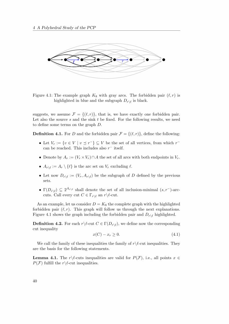
4 A Polyhedral Study of the PCP
` r`
Figure 4.1: The example graph K8 with gray arcs. The forbidden pair (`, r) ishighlighted in blue and the subgraph Dr\` is black.
suggests, we assume F = {(`, r)}, that is, we have exactly one forbidden pair.Let also the source s and the sink t be fixed. For the following results, we needto define some terms on the graph D.
Definition 4.1. For D and the forbidden pair F = {(`, r)}, define the following:
• Let Vr := {v ∈ V | v � r−} ⊆ V be the set of all vertices, from which r−
can be reached. This includes also r− itself.
• Denote by Ar := (Vr×Vr)∩A the set of all arcs with both endpoints in Vr.
• Ar\` := Ar \ {`} is the arc set on Vr excluding `.
• Let now Dr\` := (Vr, Ar\`) be the subgraph of D defined by the previoussets.
• Γ(Dr\`) ⊆ 2Ar\` shall denote the set of all inclusion-minimal (s, r−)-arc-cuts. Call every cut C ∈ Γr\` an r\`-cut.
As an example, let us consider D = K8 the complete graph with the highlightedforbidden pair (`, r). This graph will follow us through the next explanations.Figure 4.1 shows the graph including the forbidden pair and Dr\` highlighted.
Definition 4.2. For each r\`-cut C ∈ Γ(Dr\`), we define now the correspondingcut inequality
x(C)− xr ≥ 0. (4.1)
We call the family of these inequalities the family of r\`-cut inequalities. Theyare the basis for the following statements.
Lemma 4.1. The r\`-cuts inequalities are valid for P (F), i.e., all points x ∈P (F) fulfill the r\`-cut inequalities.
40

4.1 A Complete Description for one Pair
Proof. Let P be a feasible s-t-path in D and xP its characteristic vector. Theinequalities are trivially satisfied if P avoids r. Hence, let us assume r ∈ P. Inthis case P avoids `, since it is feasible. Thus, its s-r−-subpath lies completelyin Dr\` and hence intersects all r\`-cuts C ∈ Γ(Dr\`). For this reason, x(C) ≥ 1for all C ∈ Γ(Dr\`). Thus, all r\`-cut inequalities are satisfied with equality.
The next lemma is a bit more tricky. These two lemmata form the basis forthe following main theorem of this section.
Lemma 4.2. The forbidden pair inequality xl + xr ≤ 1 is implied by an r\`-cutinequality.
Proof. Recall the flow conservation Equalities (2.1) of the shortest path problemformulation for all vertices v ∈ V :
∑a∈δ+(v)
xa −∑
b∈δ−(v)
xb =
1 v = s
−1 v = t
0 otherwise
Let us now sum up the equalities for all the vertices S := {s, . . . , `−}1. Sincet /∈ S, the right side is clearly 1. All arcs appearing in the second sum are alsostarting in the set S as well and hence vanish because of the first sum. Thus,the remaining arcs are those jumping over or starting in `−. Let us give a nameto this set: T := {(a, b) | a � `− ≺ b}. Note that ` ∈ T . Of course, T is an arccut of D and hence T ′ := T ∩ Ar\` is an arc cut in Γ(Dr\`). This results in theredundant equality
x(T ) = 1. (4.2)
Consider the cut inequality of T ′, x(T ′) − xr ≥ 0. If we subtract (4.2) from it,we get
x(T ′)− x(T )− xr ≥ −1.
We know, that ` ∈ T , but ` /∈ T ′. Thus, we can summarize this to
−x` − xr − x(T \ (T ′ ∪ {`})) ≥ −1.
We see already the forbidden pair inequality appearing. Consider the negative ofthis equation
x` + xr + x(T \ (T ′ ∪ {`})) ≤ 1
and by x(T \(T ′∪{`})), this implies the forbidden pair inequality x`+xr ≤ 1.
The following theorem states the main result of this section.
1The enumeration shall be according to the topological sorting < on the graph D.
41

4 A Polyhedral Study of the PCP
` r
Figure 4.2: K8 in gray, the subgraph Dr in black.
Theorem 4.1. For one forbidden pair,
P (F) = {x ∈ P | x(C)− xr ≥ 0 ∀C ∈ Γr\`} =: Q
holds, where P denoted the solution set of the unconstrained shortest path problem.
Proof. By Lemma 4.1, we have P (F) ⊆ Q. Lemma 4.2 states, that all infeasiblepaths are excluded. Together, we have conv(Q ∩ Z|A|) = P (F). It only remainsto prove the integrality of Q.
Let therefore x∗ be a fractional vertex of Q, whose existence we have to con-tradict. Note that x∗ corresponds to a flow in D. Let us now create a new graphDr by removing ` from D as well as all arcs not lying on any s-t-path throughr. In other words, no arcs on a r+-t-path are removed and on s-r−-paths, ` isthe only arc removed. Figure 4.2 shows the graph Dr for the example K8. Thegraph Dr can be seen as an extension of the graph Dr\` to the complete vertexset V . Conversely, if we restrict Dr to the vertex set Vr, we get Dr\` again.
We now define a maximum flow problem on Dr by defining arc capacitiesca := x∗a for all arcs in A(Dr). Let xr be a maximum flow in Dr. Clearly, xr
avoids ` completely and hence can be decomposed into valid paths. The classicalmax-flow-min-cut theorem states that the value v(xr) is upper bounded by x∗r ,since {r} is an inclusion-minimal arc cut of Dr. If we can now show that v(xr)actually is x∗r , we know that the remaining flow x∗ − xr avoids r. Thus, let usfind lower bounds for v(xr).
We use the max-flow-min-cut theorem again and choose an arbitrary inclusion-minimal s-t-cut C ∈ Γ(Dr). We need to show that this cut has at least capacityx∗r . By the construction of Dr, we can distinguish three cases concerning thelocation of C.
Case 1 C disconnects s and r−. Since C is inclusion-minimal, we have C ∈Γ(Dr\`). By the cut inequality of C, we get
x∗r ≤ x∗(C) = c(C).
42

4.1 A Complete Description for one Pair
Case 2 C disconnects r+ and t. x∗ is itself a feasible flow sending a value of atleast x∗r through r+. Since this subflow also reaches t, we get
x∗r ≤ x∗(C) = c(C),
because it needs to intersect C.
Case 3 C disconnects r− and r+. C is inclusion-minimal and hence C = {r}.Of course, x∗r ≤ c(C).
This shows, that v(xr) is indeed x∗r . Thus, x` := x∗ − xr avoids r completelyand with x` and xr we found a decomposition into two feasible subflows, x`, xr ∈P (F). Since x∗ = (1−x∗r)x` +x∗rx
r is a convex combination, x∗ is also containedin P (F), which is the desired contradiction.
By this theorem we get that the forbidden pair inequalities (4.1) form a com-plete linear description of the forbidden pair polytope with a single pair, togetherwith the flow conservation constraints (2.1) and x ≥ 0.
4.1.2 One Binding Pair
The same argument flow can be translated to the problem of one binding pairB = {(`, r)} ⊆ A× A on the graph D = (V,A). Let us fix this problem instanceagain. The additional inequalities for the binding pair problem arise from arccuts as well, but we need to define a different graph before.
Definition 4.3. For D and the binding pair B = {(`, r)}, define:
1. Let V b`,r := {v ∈ V | `+ � v � r−} be the set of all vertices between the two
binding pair arcs.
2. Db`,r := (V b
`,r, (Vb`,r × V b
`,r) ∩A) The connection graph of ` and r.
3. Γ(Db`,r) shall denote the set of all inclusion-minimal (`+, r−)-arc-cuts.
Figure 4.3 shows the graph Db`,r for the example K8 again. In this example,
there are two possible minimal cuts in Γ(Db`,r), namely the two arcs starting in
`+ or the two ending in r−. Introduce the following inequalities for all cuts C inΓ(Db):
x(C)− x` ≥ 0 (4.3)
These inequalities look quite similar to the ones used for one forbidden pair,but due to the different graph construction, they fulfill our needs, as we will seeshortly. In addition to these cut inequalities, we need the binding pair inequality
xr − x` ≥ 0 (4.4)
to describe the polytope P (B). This section goes alike the last one and the proofsdiffer only slightly.
43

4 A Polyhedral Study of the PCP
` r
Figure 4.3: K8 in gray, the subgraph Db`,r in black.
Proposition 4.1. The inequalities (4.3) and (4.4) are valid for P (B) and allinfeasible paths violate the binding pair inequality (4.4).
Proof. Take any feasible path P and its characteristic vector xP . If it avoids `then the inequalities are trivially satisfied. So let us assume xP` = 1. Since P isfeasible, it also uses r and the binding pair inequality is valid again. And sinceboth ` and r are used, the path needs to go from `+ to r−, which is clearly inDb`,r. Here, it intersects all cuts and thus the cut inequalities are also valid.Let P be infeasible now. The binding pair (`, r) can only be violated if P uses
`, but not r. In this case, xPr = 0 and xP` = 1, which obviously violates thebinding pair inequality.
With these two results we are in the same situation as before and now able tostate the theorem.
Theorem 4.2. For D = (V,A) and B = {(`, r)},
P (B) = {x ∈ P | (4.3), (4.4)} =: Q
holds.
Proof. The proposition tells us P (B) ⊆ Q and no additional integral points belongto Q. Thus, the only possibility is an additional fractional vertex x∗ of Q whoseexistence we have to contradict: Let Db be a new subgraph of D on the samevertex set. A(Db) shall be the union of all s-t-paths using both ` and r. Db
restricted to [`+, r−] is precisely the graph Db`,r. Note, that both {`} and {r} are
arc cuts in Db. Figure 4.4 illustrates Db.On this graph, we are now interested in maximum flows. The capacities on the
arcs shall be ca := x∗a and let x be a maximum flow in Db. Of course, x uses both` and r, since they are cuts. x∗ was a point in Q and hence it satisfies xr ≥ x`.x∗` is again an upper bound for v(x). We will now show, that x∗` = v(x) using themax-flow-min-cut theorem. Let C be any inclusion-minimal cut in Γ(Db). Wecan distinguish several cases regarding the allocation of C on Db.
44

4.1 A Complete Description for one Pair
` r
Figure 4.4: K8 in gray, the subgraph Db in black.
Case 1 C disconnects s and `− or r+ and t. Since x∗ is a feasible flow andno arcs between s and `− (respectively r+ and t) are removed, it must bepossible to send an amount of x∗` through C (respectively, the same holdsdue to the binding pair inequality (4.4) for the case C disconnects r+ andt). Thus, x∗` ≤ x∗r ≤ c(C).
Case 2 C disconnects `+ and r−. Then, C ∈ Γ(Db`,r) and the corresponding cut
inequality holds for x∗. Thus,
x∗` ≤ x∗(C) = c(C)
Case 3 C ∈ {{`}, {r}}. In this case, c(C) = x∗` or c(C) = x∗r . By the bindingpair inequality we get again x∗` ≤ c(C).
This shows that the subflow x of x∗ uses the whole of x∗ on ` and the remainingflow x′ := x∗ − x avoids ` completely. In addition, the whole flow x uses r andhence, the both subflows x and x′ are feasible concerning B and since x∗ =(1− x∗` )x′ + x∗`x is a convex combination, all the three points x, x′ and x∗ are inP (B). This contradicts the assumption, that x∗ is a fractional vertex of P (B).
This is the same result as for a forbidden pair: The inequalities (4.3) and (4.4)form a complete linear description of the polytope associated with the shortestpath problem with pair constraints for the case of one binding pair (`, r).
4.1.3 Separation and the Number of Facets
As the complete linear descriptions derived in the previous sections suggest, thenumber of inequalities needed to describe the polytope can be very large. We arenow going to show, that it can actually grow exponentially large. We show thisfor the special case of a complete graph D = (V,A) and one forbidden pair (`, r).
Definition 4.4. Define the following:
45

4 A Polyhedral Study of the PCP
• Let Π be the set of infeasible paths in D using both ` and r.
• For I ∈ Π, let
CI,`,r := {(u, v) ∈ Ar\` | `+ � v � r−, u /∈ Iv, v ∈ Iv}
be the cut associated to this infeasible path. Note that CI,`,r ∈ Γ(Dr\`)for all I ∈ Π. This cut can be seen as all the arcs “entering” the path Ibetween `+ and r−.
• Let [u, v] := {x ∈ V | u � x � v} be the set of all vertices between u and vand P[u, v] the subpath of a path P between u and v.
• Let P and Q be two inner vertex-disjoint u-w-paths. We call the unionP ∪Q a (u,w)-split. For two s-t-paths, let s(P,Q) be the number of splitsin P ∪Q for which Q has at least one inner vertex.
With these definitions, we can now formulate the following theorem.
Theorem 4.3. Let I ∈ Π. Then, the r\`-inequality associated to CI,`,r, i.e.,
xr ≤ x(CI,`,r) (4.5)
defines a facet f(P) ⊆ P (F). Furthermore, two different paths I1, I2 ∈ Π definedifferent facets of P (F), f(I1) 6= f(I2).
For an infeasible path I ∈ Π, let ΠI be the set of feasible s-t-paths in D whichare tight for xr ≤ x(CI,`,r). The proof of this theorem gets quite technical. Forthis reason, let us outsource a useful claim. Recall, that Pv denotes the set ofvertices of a path P.
Lemma 4.3. Let I ∈ Π. A feasible path Q satisfies the inequality xr ≤ x(CI,`,r)with an equality if and only if one of the following holds:
(I) Q avoids both ` and r and Iv ∩Qv ∩ [`+, r−] = ∅.(II) Q contains either ` or r and s(I,Q) = 0.
Proof. Let us prove the lemma separately for the cases of whether arcs ` and rare used by Q. Let therefore I ∈ Π be fixed and take Q a feasible path whichavoids ` and r. Assume, Q satisfies the inequality with equality. Since xQr = 0,we need to contradict the existence of a vertex in Iv ∩Qv ∩ [`+, r−]. Assume thisvertex w exists. Since Q avoids `, but meets I in w, there needs to be an enteringarc, Q uses to meet I. Let this arc be (u, v). Possibly, but not for sure, we havev = w here. Since Q avoids r, there cannot be an equation in the cut equality,which is the desired contradiction. The opposite direction works similar: If thereis no vertex v ∈ Iv ∩ Qv ∩ [`+, r−], Q cannot visit any arc in CI,`,r and hencex(CI,`,r) = 0.
Let Q now visit ` and fulfill the r\`-cut inequality with equality. Q is feasibleand hence avoids r. Thus, we need to show, that there is no (u,w)-split (with
46

4.1 A Complete Description for one Pair
an inner vertex on Q \ I) in I ∪ Q with u,w ∈ [`+, r−]. Assume, there is such a(u,w)-split. Let v be the largest vertex on Q before w. As assumed, u ≺ v ≺ wand hence v ∈ Q \ I. Thus, (v, w) ∈ CI,`,r and we are ready. For the backwardsdirection, let Q have s(I,Q) = 0. Assume there is an arc (v, w) ∈ CI,`,r visitedby Q. Let u be the largest vertex before v that I and Q share. Since Q visits `,`+ ≤ u and hence I[u,w] ∪ Q[u,w] is a (u,w)-split in [`+, r−], which has to becounted in s(I,Q), a contradiction.
As the last case, let Q visit r with an equality in the cut inequality. Assumeagain the existence of an (u,w)-split in I ∪ Q with u,w ∈ [`+, r−]. Let (v, w) bethe arc of Q ending in w. This arc is of course contained in CI,`,r. But sinceQ avoids `, there have to be at least two arcs in CI,`,r, which uses Q. This isthe desired contradiction. Let now g be the smallest vertex I and Q share with`+ ≤ g. Since Q avoids `, the arc (f, g) (with the proper vertex f) of Q is alsocontained in CI,`,r. Thus, the sum of Q over this cut is at least two, which isa contradiction. Finally, let there be no split between I and Q in [`+, r−]. Inthis case, the both paths meet only once between `+ and r− and hence there isonly one entering arc (u,w) ∈ CI`,r used by Q, which leads us to the desiredequality.
Since the dimension of the polytope P (F) is completely unknown to us, we arenot able to say anything about the co dimension of a face of it. This is why weapply a non-standard proof technique here. We show that
P (F) ⊆ aff({xQ} ∪ f(I)) (4.6)
holds for every infeasible path I ∈ Π and every feasible path Q, which is nottight for the inequality associated to I. This is possible by the following lemma.
Lemma 4.4. Let I ∈ Π be an infeasible path and Q ∈ P (F) \ f(I) a feasiblepath not tight for the inequality of I. Then, we can find the following affinecombination
xI = λQxQ +
∑P∈ΠI
λPxP
of xI with λQ+∑P∈ΠI
λP = 1. In particular, if Q belongs to case I of Lemma 4.3
then λQ = − 1s(I,Q) , while for case II λQ = − 1
s(I,Q)+1 holds.
This lemma is quite complicated. After its proof, the proof of Theorem 4.3finally follows. There is explained, how we can use this unexpected affine combi-nation for proving (4.6).
Proof. For this proof, fix the infeasible path I ∈ Π. Since for every path Q, thenumber s(I,Q) is constant, we do an induction over this number. In other words,we find the desired affine combination with Q using other affine combinations ofpaths with a lower split number.
47

4 A Polyhedral Study of the PCP
u` rI I
Q Q
Figure 4.5: The infeasible path I uses both ` and r, whereas Q avoids both. Thetwo paths meet in their only common point u.
Let us begin the induction with the cases s(I,Q) = 0. Take a path Q, which isnot tight for the cut inequality associated to I, see Figure 4.5. By Lemma 4.3, Qavoids both ` and r. The lemma further tells us, that there is a common vertexu of the paths I and Q. The affine combination is
xI = (xI[s,u] + xQ[u,t])
+ (xQ[s,u] + xI[u,t])
− x(Q).
The two new paths are rearrangements of I and Q at u. Obviously, both arefeasible. It remains to check, that they are tight for the considered inequality.This can – in this case and in the plenty following ones – be easily checked bylemma 4.3.
To facilitate the induction step, we also give the induction start for the cases(I,Q) = 1 and start the induction with at least two splits. We need to distin-guish three cases for Q. Let S be the given (u,w)-split and let v be a node in(Q \ I) ∩ S.
1. Q contains neither ` nor r.
xI =1
2(xI[s,u] + xQ[u,v] + x(v,t))
+1
2(x(s,v) + xQ[v,w] + xI[w,t])
− 1
2(x(s,v) + x(v,t))
+1
2(xQ[s,u] + xI[u,t])
+1
2(xI[s,w] + xQ[w,t])
− 1
2xQ
48

4.1 A Complete Description for one Pair
2. Q contains ` but not r.
xI = (xQ[s,w] + x(v,t))
+ (x(s,v) + xQ[v,w] + xI[w,t])
+ xI[s,w] + xQ[w,t])
− (x(s,v) + x(v,t))
− xQ
3. Q contains r but not `.
xI = (xQ[s,u] + xQ[u,t])
+ (xI[s,w] + xQ[u,v] + x(v,t))
+ (x(s,v) + xQ[v,t])
− (x(s,v) + x(v,t))
− xQ
Here, the new paths are similarly to the ones of s(P,Q) = 0 generated. Fig-ure 4.6 illustrates the three situations. At this point we need that D is thecomplete graph, which guarantees us the existence of the arcs (0, v) and (v, n).
The induction step uses the same argument of rearranging the paths. We againneed to distinguish the same cases as above, which will be as similar as the aboveones. For this reason, we will completely prove the first one. For the other two,we only show the differences in the construction of the new paths.
As induction hypothesis, assume that the claim holds for all paths Q′ withs(I,Q′) ≤ k − 1. Let therefore Q be a feasible path, which is not tight for thecut inequality of CI,`,r and with s(I,Q) = k. Let for all cases the vertices u andw define the smallest (u,w)-split of I ∪Q and let v be an inner vertex on Q \ I.
Case 1: Q avoids both ` and r
We can reformulate xQ as
xQ = (x(s,v) + xQ[u,t]) =: Q1
+ (xQ[s,u] + x(v,t)) =: Q2
− (x(s,v) + x(v,t)). =: Q3
Table 4.1 on page 51 lists some properties of the paths Q1, Q2 and Q3, which caneasily be verified in Figure 4.7. The table shows that for Q1 and Q2 the inductionhypothesis holds, which leads us to the following two affine combinations for xI .
xI = −1
kxQ1 +
∑P∈ΠI
λ1PxP (4.7)
49

4 A Polyhedral Study of the PCP
u
v
w` rI I
Q
I
QQ Q
(s, v) (v, t)
u
v
w` rI I
Q
I
Q
Q
Q
(s, v) (v, t)
u
v
w` rI I
Q
I
QQQ
(s, v) (v, t)
Figure 4.6: The three cases for s(I,Q) = 1.
xI = −xQ2 +∑P∈ΠI
λ2PxP (4.8)
With ∑P∈ΠI
λ1P = 1 +
1
kand
∑P∈ΠI
λ2P = 2. (4.9)
Let us now compute the equation [k · (4.7) + (4.8)].
(k + 1)xI = −xQ1 + k ·∑P∈ΠI
λ1PxP − xQ2 +
∑P∈ΠI
λ2PxP
From the construction of the paths Qi we know xQ = xQ1 + xQ2 − xQ3 . Let usreplace −xQ1 − xQ2 in the last equation by −xQ − xQ3 and divide it by (k + 1)
50

4.1 A Complete Description for one Pair
u
v
w`r
Q
I
Q
I
Q Q
I· · ·
Q
I
Q
I
(s, v)
(v, t)
Figure 4.7: Q avoids both ` and r and s(I,Q) = k.
Path Tight for I Number of Splits Case (Lemma 4.3)
Q1 not tight s(I,Q1) = k − 1 Case IQ2 not tight s(I,Q2) = 0 Case IQ3 tight s(I,Q3) = 0 Case I
Table 4.1: Properties of the three new paths Q1, Q2 and Q3 for Q avoiding both` and r.
to get
xI = − 1
k + 1· xQ − 1
k + 1· xQ3 +
k
k + 1·∑P∈ΠI
λ1PxP +
1
k + 1·∑P∈ΠI
λ2PxP
= − 1
k + 1· xQ − 1
k + 1· xQ3 +
∑P∈ΠI
(k · λ1
P + λ2P
k + 1· xP
). (4.10)
Obviously we approach an affine combination of xI with xQ and the vertices inf(I). By Table 4.1 we know that Q3 is tight for the inequality to CI,`,r and henceappears as a path P ∈ ΠI in the sum. This gives rise to a definition of the newaffine combination coefficients λP . Define for P ∈ ΠI the coefficient
λP :=
{k·λ1P+λ2Pk+1 P 6= Q3
k·λ1P+λ2P−1k+1 P = Q3.
It is easy to see, that the affine combination (4.10) transforms into
xI = − 1
k + 1· xQ +
∑P∈ΠI
λPxP
51

4 A Polyhedral Study of the PCP
Path Tight for I Number of Splits Case (Lemma 4.3)
Q1 not tight s(I,Q1) = k − 1 Case IIQ2 not tight s(I,Q2) = 0 Case IQ3 tight s(I,Q3) = 0 Case I
Table 4.2: Properties of the three new paths Q1, Q2 and Q3 for Q using ` butnot r.
using the new coefficients λP . This is precisely the combination we wanted toachieve. The last point to verify is now, that this is actually an affine combina-tion, i.e., ∑
P∈ΠI
λP =k + 2
k + 1.
This is achieved in the following calculation. The equality (∗) uses, that the twoformulations using Q1 and Q2 were affine combinations as well. Formally, thiswas stated in (4.9).
∑P∈ΠI
λP =∑P∈ΠI
k · λ1P + λ2
Pk + 1
+1
k + 1=
1
k + 1·
k · ∑P∈ΠI
λ1P +
∑P∈ΠI
λ1P − 1
∗=
1
k + 1·[k(1 +
1
k) + 2− 1
]=k + 2
k + 1
Case 2: Q uses either ` or r
The computations for this case go quite similar to the last one. Mainly theexact formulation of the coefficients λP differs. This is why we omit the repeatedcalculation. Instead we just give an explanation, how we rearrange the paths andwhich properties they have.
At first, let Q visit ` and not r. We do the same construction as before:
xQ = (x(s,v) + xQ[u,t]) =: Q1
+ (xQ[s,u] + x(v,t)) =: Q2
− (x(s,v) + x(v,t)). =: Q3
Table 4.2 lists the properties of the three paths Q1, Q2 and Q3. Note, that Q1
is in this case of type II concerning Lemma 4.3. For type II, the coefficient of Qhas to be − 1
s(I,Q) instead of − 1s(I,Q)+1 for type I.
The last case, that Q uses r looks similar, but here Q2 is of type II. The lattertwo are visualized in Figure 4.8. All three cases together prove the induction andhence the lemma.
52

4.1 A Complete Description for one Pair
u
v
w`r
QI
Q
I
Q Q
I· · ·
Q
I
Q
I
(s, v)
(v, t)
u
v
w`r
Q
I
Q
I
Q Q
I· · ·
Q
I I, Q
(s, v)
(v, t)
Figure 4.8: Q meets ` above and r below. In both cases, we have s(I,Q) = k.
With this lemma, we can now prove the theorem.
Proof of theorem 4.3. Actually, Lemma 4.4 tells us xI ∈ aff({xQ}∪ f(I)), whichis the same as
xQ ∈ aff({xI} ∪ f(I)).
This can be achieved by a taking an affine combination of xI and solving theequation for xQ. It can be easily seen that the result is again an affine com-bination. Since this holds for every feasible path Q, we can use two of theseexpressions
xI ∈ aff({xQ1 } ∪ f(I)) (4.11)
xQ2 ∈ aff({xI} ∪ f(I)) (4.12)
for different paths Q1 and Q2 to get the final expression
xQ2 ∈ aff({xQ1} ∪ f(I))
we originally searched for. This is easy to verify by taking an affine combinationof xI from (4.11) and plugging it into one of xQ2 of (4.12). The result is clearlyan affine combination of xQ2 in aff({xQ1} ∪ f(I)). Since the latter holds for allQ2 with a fixed path Q1, we can conclude
P (F) ⊆ aff({xQ1} ∪ f(I)).
53

4 A Polyhedral Study of the PCP
The theorem allows a direct corollary, since there are exponentially many sub-paths between `+ and r−.
Corollary 4.1. The number of facets of P (F) is exponential in the number ofvertices |V |.
We have now seen, that the description of the convex hull of P (C) can growexponentially large. But this is not a hard problem because of the followingresult.
Proposition 4.2. The system of inequalities
{x ∈ R|A| | (4.1), (2.1), x ≥ 0}
in the case of one forbidden pair or
{x ∈ R|A| | (4.3), (4.4), (2.1), x ≥ 0}
for a binding pair can be separated in polynomial time.
Proof. Let x∗ ∈ R|A| be the point to be separated. Since (2.1) together withx ≥ 0 describe a flow problem and the number of these constraints is polynomial,we can assume that x∗ ∈ P , that is, x∗ defines an (s, t)-flow of value 1. Otherwise,we can easily find the violated constraint.
Consider the case of one forbidden pair. Create the graph Dr according to theproof of Theorem 4.1 and use x∗ as capacities for the arcs. Let x′ be a maximum(s, t)-flow over Dr satisfying these capacities. Assume the value v(x′) is equalto x∗r . That means by the max-flow-min-cut theorem that the capacity of every(s, t)-cut in Dr is at least x∗r . As all cuts in Cr\` are fully contained in Dr, allr\`-cut-constraints (4.1) are satisfied. Contrarily, if the value of x′ is strictlysmaller than x∗r , then there must exist a bottleneck corresponding to a cut withcapacity smaller than x∗r . Clearly, this cut belongs to Cr\`. And the correspondinginequality (4.1) is violated in this case.
The case of a binding pair can be proven by the same idea. In this case, thegraph construction of the binding pair section is needed here. By this method wecan separate the given inequality system in polynomial time.
Obviously, the same result holds also for problem instances with exactly onebinding pair.
4.2 Contiguously Disjoint Pair Constraints
This section extends our results to a first simple case of multiple constraints.
54

4.2 Contiguously Disjoint Pair Constraints
Definition 4.5. The set C is called contiguously disjoint if the following conditionis satisfied:
s � `−1 ≺ `+1 � r
−1 ≺ r
+1 � . . . � `
−k ≺ `
+k � r
−k ≺ r
+k � t
In this case, for the complete linear description, there are no more inequali-ties needed than the ones we got by each pair constraint for itself presented inSection 4.1.
Theorem 4.4. Let C be a set of contiguously disjoint pair constraints. Then thefollowing holds:
P (C) =
k⋂i=1
P (Ci).
In this proof, we need to be careful, whether the considered constraint is aforbidden pair or a binding pair.
Proof. A great advantage of the proof in Section 4.1.1 for a forbidden pair is thatLemma 4.1 and Lemma 4.2 can be easily extended to the more general case ofmultiple pair constraints: They guarantee that all path vertices respecting theappropriate forbidden pair are kept in the new polytope P (C) and that all invalidones are eliminated by the r\`-inequalities. An analogous argument holds for abinding pair with Proposition 4.1. This is independent of other constraints in C.So again, the only point left to prove is the following lemma.
Lemma 4.5. The polytope⋂ki=1 P (Ci) is integral.
Proof. Our proof takes an inductive approach over the number of considered pairconstraints. Let C≤i :=
⋃ij=1 Ci. The induction hypothesis is: P (C≤i−1)∩P (Ci) =
P (C≤i) and P (C≤i) is integral. The induction start is already given in Section 4.1.1for a forbidden pair and in Section 4.1.2 for a binding pair. Let us now solve theinduction step.
The direction P (C≤i−1)∩P (Ci) ⊇ P (C≤i) directly follows by the definition. Forthe converse, let us take a fractional vertex x∗ in P (C≤i−1)∩P (Ci) and contradictits existence. We are going to see that x∗ is contained in P (C≤i) by expressing itas a convex combination of points in P (C≤i).
By using the split method from Sections 4.1.1 or 4.1.2, we can split the flowx∗ into two flows x∗ = x1 + x2. For a forbidden pair, let x1 = x` and x2 = xr.For a binding pair, let x1 = x and x2 = x′. In both cases, x1 and x2 are flowsrespecting Ci.
Consider now the set C := {(u, v) ∈ A | u � `−i ≺ v}. Clearly, this set is anarc cut of D and since every arc in C is either jumping over `−i or starting in`−i , no path can intersect C twice. Let us consider now path decompositions ofthe three points x, x1, x2 and call them M , M1 and M2, respectively. Clearly,M1∪M2 is a path decomposition of x as well, but in general a different one thanM .
55

4 A Polyhedral Study of the PCP
Let us now take a closer look at C. This cut separates the first i− 1 forbiddenpairs from the i-th one, because C was contiguously disjoint. M is a path decom-position, where all paths respect the first i − 1 forbidden pairs, and M1 ∪M2
a path decomposition respecting the i-th one. And clearly, both decompositionsuse C in the same amounts per arc. Since all the decompositions are clearlyfinite, we can compute a new decomposition of x by mixing the left part of Mwith the right part of M1 ∪M2: For every arc a ∈ C, consider all paths in M(and M1∪M2) using a. By arranging new paths out of the 0-a−-subpaths of thepaths in M , the arc a itself and the a+-n-subpaths contained in M1∪M2, we getour new decomposition, called M∗. The paths in M∗ respect all pair constraintsin C≤i and hence, x∗ is a convex combination of these valid paths. That is, x∗ iscontained in P (C≤i). Since x∗ was fractional, M contained at least 2 paths andhence, x∗ is no vertex, which is our desired contradiction.
56

5 Computational Results
This chapter presents our algorithm introduced in chapter 3 on page 29 in apractical way. We implemented the method contractGraph and tested it onseveral instances. The following section gives a short introduction to the code ofour software and the workaround that comes with it. Then, we explain, why wedecided not to consider obligatory pairs. Sections 5.3 and 5.4 explain the real-world data, how we transformed them into instances of the shortest path problemwith pair constraints and which test instances we chose. Finally, Section 5.5harvests some pictures of flight trajectories and evaluates the calculation timesand some more details to the calculation in a practical view.
5.1 Implementation
We decided to implement an environment for the pair constraint contractionalgorithm in the programming language C++. In 9 files with a total of 3222 lines,we implemented 15 classes. The environment consists of several components,which we will present in the following paragraphs.
The first isolated part is a priority queue supporting a decreaseKey operation.The built-in priority queue of C++ does not provide a decreaseKey operation. Apriority queue is a data structure supporting easy access to the first – or smallest– element. Each element has an integer key, which is used to compare them todetermine the smallest element. The method decreaseKey resorts the queue,after the key of one element decreased. This is required for Dijkstra’s Algorithm.Our PriorityQueue<Item> class is implemented as a binary heap, which is itselfstored in a vector object. A good introduction to the priority queue and itsimplementation based on an array can be found in [9, 17].
We implemented an environment handling directed graphs. This consists ofclasses for vertices, arcs and directed graphs as well as an own class representing adistance label for Dijkstra’s Algorithm. Of course, this algorithm is implementedin this environment as well as Algorithm 1 for a topological sorting. Our graphis stored in a doubly connected edge list (DCEL). This means, that every vertexstores one incoming and one outgoing arc. Every arc then stores a link to the nextoutgoing arc or to the next incoming arc. This structure allows easy navigationin the graph, especially for rule R2’.
To handle the vertex pair constraints, we built a second couple of classes ex-tending the previously mentioned ones. These classes now support forbidden andbinding pairs and the contractGraph algorithm presented in Chapter 3.
57

5 Computational Results
This setting is surrounded by a management software, which allows the easycreation, preparation, and deletion of problem instances. This part also runsthe contractGraph method and measures its result as well as some parametersdescribing the performance. This will be explained further in section 5.5.
Every vertex gets a unique id of type unsigned short integer needing only twobyte rather than four compared to normal integers. Unsigned short integers havea range of {0, . . . , 216 = 65536}. As we will see, we need to treat around 48.000vertices and hence this range is perfect for vertex ids. The basic contractGraph
algorithm only determines whether there is a feasible path respecting all pairconstraints or not. To actually find such a path, we need a slight modificationof the graph. Every arc gets a label consisting of a list of vertex ids (unsignedshorts). By default, every label of arc (x, y) begins with the id of x followed bythe id of y. The new arc (x, z), which arises from the contraction of y by the arcs(x, y) and (y, z) gets the concatenation of their two labels as new label1. By thisway, we keep the information, which arcs and vertices this new arc represents.By iterating this, we always keep track of the shortest path in the original graphD connecting the two vertices x and z. Thus, the final label of the potential arc(s, t) explains the shortest trajectory respecting C.
Summarized, our data structure for an arc (x, y) contains the following infor-mation:
• Pointers to the two vertices.• A pointer to the next outgoing arc of x.• A pointer to the next incoming arc of y.• The arc weight (its length).• The arc label.
The four pointers use 32 bit each as well as the weight, which is stored as aninteger. The label contains all the vertices this arc shall connect stored as a listof ids. This leads to a bare minimum of 56 byte per arc, which is found by thesizeof command of C++. This is aggravated by the ids contained in the labelof (x, y). The label sizes of course increase during the process of the algorithm.Typical arc label sizes are around 200 near the end of a run of contractGraph.
5.2 Extension to Obligatory Pairs
To get the method contractGraph to handle also obligatory pairs, the rule B2
has to be altered to handle the new case of an obligatory pair. To force a paththrough at least one of two contiguous vertices in a topological sorted graph, weneed to remove all arcs jumping over both a and b, see Figure 5.1. To achievethat in a DCEL, we needed to modify our connection structure in a manner, thatnot only incoming and outgoing arcs are saved at each vertex, but also jumping
1Acually, in this case, every vertex id is stored twice in the list, because the first arc label endswith the id of y and the second label begins with it. But this can clearly be avoided bysimply removing this repeated id
58

5.3 A Translation Heuristic for Traffic Flow Restrictions
a b
Figure 5.1: The two black arcs need to be deleted to enforce a feasible path touse at least one of the two vertices of the obligatory pair (a, b).
arcs. Since this jumping is only defined using a topological sorting in contrast tooutgoing and incoming arcs, this caused problems to us. This is why we omittedobligatory pairs in this thesis.
5.3 A Translation Heuristic for Traffic Flow Restrictions
As already mentioned in the beginning, the RAD document contains tons of rulesto be respected by passenger airplanes flying through the airway network graph.Table 5.1 on the next page shows a little excerpt of the RAD document. Thereare some columns dropped for the example and some of the arount 10.000 rowschosen to give an example. Within this context, vertices are called waypoints andarcs are called segments.
Waypoints in the airway network graph always have a name consisting of fiveuppercase letters. Airports have possibly shorter names. Every line in the RADdocument table stands for one specific rule and every rule always has to be appliedfor every single flight itself. Every rule consists of three parts, namely the scope,the condition and an order. The first column “from – to” contains the scope, inthis case a segment. There are also other scopes. The rule dictates somethingconcerning this scope. The second column contains the condition and the order.The condition makes clear, whether this rule is active for the current flight or not.Usually, it is beginning in the second line. The first line contains the order. It tellsus, what actually holds for the scope if the condition is satisfied. For the order,there are three types used in the document: Compulsory, not available and onlyavailable. Compulsory rules force us to use the scope if the condition is satisfied.Contrarily, not available rules forbid the scope in this case and in only availablerules, we are not allowed to use the scope if the condition is not fulfilled. Thescope mostly contains a single waypoint or a single segment. Sometimes, there isa height condition given to the scope as well or a complete airway consisting ofmultiple contiguous segmentss.
The difficult part is the condition. As seen in the examples, a condition is aboolean expression containing various types of properties a trajectory can have.Let us call these types literals for now. The literals are in general:
59

5 Computational Results
From – to Restriction Id No.
RANUX – VALEK Not available for trafficARR EDDF/FEVia BETEXAbove FL245
LF2935
EPOLO – DIVKO Only available and compulsory for trafficDEP LFMNVia MAMES/NILDU/VATIRWith RFL above FL195
LF2756
NINTU – MEBAK Only available for traffic
1. Via OLRAK2. Via TIS
a) DEP Geneva Areab) DEP EDDM, LFSB
With ARR Bordeaux Groupc) DEP ED**, LS**, LO**
With ARR NAT3. ARR Clermont Ferrand Group,
Limoges Group, Poitiers Group
LF2313
Table 5.1: Some example rules taken from [11].
• Arrival or departure (DEP, ARR)• Using a waypoint (VIA)• Using an airspace (VIA)• Using a waypoint starting with a certain prefix• Using an airway containing given contiguous segments• Using an airplane of a certain type• Equipment properties• Flight in a certain range of altitudes• Flying in a certain time interval of the day
Of course, some of these types are constant once we chose an instance tocompute. This holds e.g. for arrival, departure, equipment or the airplane type.The airplane type distincts for example between propellor maschines or jet planes.Other types are dynamicly depending on the chosen trajectory, such as the VIAconditions for example. The last two, namely the height or time intervals, alwayspoint only to a certain part of the trajectory such as a waypoint or an airspace.
The literals are combined to a Boolean expression by typical operators such
60

5.3 A Translation Heuristic for Traffic Flow Restrictions
Oder
AND
SAND
ALGHeight
0 - 9500 FF
ARR
EDJA
MILKA
Figure 5.2: Example of a Boolean expression tree scope or condition.
as and, or and not. For the two intervals, there was a new operator invented:sand. sand connects a height or time interval with one of the other literals andthis shall evaluate to true if the interval is respected at the specified literal.
The same operators are allowed for the scope as well. Thus, a rule consistsof two Boolean expressions scope and condition and an order. Currently, theyare implemented as a binary tree, see Figure 5.2 for an example tree. If a rulein the RAD document consists of two orders, it can be split into two rules withone order each. This is for example the case in the third rule in Table 5.1. Thismodel is the state of the art of the development at Zuse-Institute Berlin for theoptimization software for flight trajectories.
The three order types are directly related to forbidden and binding pairs. Acompulsory rule is clearly a binding pair, a not available rule is a forbidden pair.And an only available rule can also be seen as a binding pair. If we want touse the scope, we need to satisfy the condition. Thus, to reduce these rules toour model of forbidden and binding pairs, the crucial point is the extraction ofconcrete waypoints from a condition or scope tree.
We solved this problem just by a heuristic. Thus, we have no guarantee, thatall forbidden and binding pairs represent the rules in a good manner. It turnsout that about 75% of the rules depend on the departure or arrival. This is thefirst step our heuristic checks. Then, our heuristic simply collects all waypointids of via nodes or airway nodes, which are contained in the Boolean expressions.Often, they contain multiple waypoints (e.g. the second rule in Table 5.1) andhence, the reduction to a vertex pair constraint is abiguous. To keep the heuristiceasy, it searches for the very first pair of distinct ids from scope and condition.
61

5 Computational Results
The following numbers belong to the instance Sydney to Peking, but the num-bers differ only very slightly between the remaining instances. From 8404 re-strictions currently loaded in the software, there are 809 binding pairs and 646forbidden pairs parsed. 6162 restrictions depend on an origin different from Syd-ney or on a destination different from Peking and hence are not active for thisinstance. 755 rules are not concerned with explicit graph elements, but with hugeairspaces or other conditions. Hence, they can not be modelled as dynamic ruleson the graph on the level of segments and waypoints. The last 32 restrictionsare concerned with explicit waypoints, but combining it with a height condition,e.g. “If you use waypoint x, use it above flight level 265”. These are modelled ascompulsory restrictions. Their condition only contains waypoint x, but the scopehas “x sand above flight level 265”.
This heuristic lets one point open. Of course, these restrictions have a pri-ori none of the structure properties presented in section 2.2.3. To achieve this,we formulated an auxiliary integer program. Once the graph is topologicallysorted, we can construct a conflict graph G, where the vertices are the vertexpair constraints and an edge is inserted if two pairs halve each other. Considerthe following integer program:
maximize z =∑c∈C
xc
subject to xc1 + xc2 ≤ 1 ∀(c1, c2) halving
xc ∈ {0, 1} ∀c ∈ C
Our software solves this integer program using the integer program solver SCIP.The solution corresponds to a maximal independent set in G, which itself is awell-paranthesized subset of C. Now, our instance is ready to be solved as ashortest path problem with vertex pair constraints.
5.4 Test Instances
For our test purposes, we picked eight airports worldwide and considered all 56possible flights between them. The airports are:
1. Atlanta (ATL)2. Paris (CDG)3. Dubai (DXB)4. Frankfurt (FRA)5. Los Angeles (LAX)6. London (LHR)7. Peking (PEK)8. Sydney (SYD)We wanted to spread them over the whole world and that we have various
different distances between them. The restrictions in the RAD document are
62

5.5 Results
0 5 10 15 20 25 300
500
1000
1500
Million Inserted Arcs
Ru
nn
ing
Tim
ein
Sec
ond
s
Figure 5.3: The running times depending on the number of inserted arcs.
mostly based in Europe. This is why we tried to have several distances includingEurope and others avoiding Europe.
5.5 Results
We started the computations on a DELL Precision 650 machine with 32 ker-nels having 2.7 GHz each. The machine has 64 Gigabyte RAM internal mem-ory running Ubuntu Linux 14.04. For each of the 56 instances, we started thecontractGraph tool. For comparison, we also started SCIP with the initial IPformulation of the shortest path problem with pair constraints. The result tablescan be found in Section 7.1. Table 7.1 lists all running times as well as the sizeand length of the result trajectories and the instance sizes. In all 56 instances,the trajectories found by contractGraph and SCIP for the same problem instancewere identical.
Unfortunately, the scip computations are essentially faster than the ones ofour method contractGraph. An interesting result is the column of inserted arcs.This value counts the number of arcs inserted by the application of rule B2.Figure 5.3 shows the dependency of the running time to the number of insertedarcs. The chart suggests that there is a more than linear dependency of therunning time by the number of inserted arcs. The instances are of almost equal
63

5 Computational Results
Figure 5.4: Snippet of the trajectories From Paris to Dubai. The right one isunconstrained, the left one respects C. The black boxes mark theresponsible binding pair. The picture is made using SkyVector.
size in all of the three data types vertices V , arcs A and constraints C. However,the newly inserted arcs range from 2 millions to over 30 millions. As seen, an arccosts at the very least 56 byte and hence we have more than a Gigabyte mainmemory usage here. The final trajectories contain up to over hundred verticesand hence all the arc labels have sizes in this scale. This justifies the exorbitantmemory usage of contractGraph of around 10 Gigabytes or more.
An interesting fact concerns the instance Atlanta to Los Angeles and its back-wards direction. The result trajectory here uses only 4 or 5 vertices, but coversa distance of over 3.000 kilometers. The reason for this is, that there are twotypes of arcs used in the graph. The first one are the normal arcs between thewaypoints, ususally in a certain height. The second type are so-called terminalprocedures, which connect the airports to several vertices in the graph. Thesearcs shall represent diffenrent landing or starting routes. Some of these arcs arereally long and in this concrete case, the found trajectory only consists of terminal
64

5.5 Results
Figure 5.5: The trajectories From Peking to Frankfurt. The lower one is un-constrained, the upper one respects C. The picture is made usingSkyVector.
procedures.We compared the result trajectories to the unconstrained shortest path through
the airway network. Figure 5.4 shows a typical result. We see here the local natureof the pair constraints. The snippet is taken from the result trajectories from Paristo Dubai and shows the Persian Gulf. The right trajectory is just the shortestpath not respecting any pair constraint. The black squares mark a binding pair.At the black square, the trajectory needs to turn left to Khark Island transformingit into a detour. For this reason, the feasible shortest trajectory avoids the bothsquares. Sometimes, the influence of the pair constraints is a bit more global, seefor example Figure 5.5. In this case, the constrained trajectory (the upper one)takes a completely different route than the unconstrained one. Reason for thisis just one forbidden pair shortly before they meet above Leipzig. A surprisingfact is that these two trajectories differ by only 10 kilometers which is less than0.2% of the trajectory length. The second table in Section 7.1 compares allresult trajectories with the shortest path through the airway network. For mostinstances, the length difference is negligible, but sometimes, the values differ upto over 100 kilometers for example from Atlanta to Peking.
65


6 Concluding Remarks
In this thesis, we tried to approach the shortest path problem with pair con-straints. We collected literature to the problem and found a formalism, whichallows to formulate both the problems already considered in the literature and theconcrete problem, we were concerned in our research. This includes behaviours ofthe problem under particular restrictions and the connections between these re-strictions as well as hardness results for each of them. Furthermore, we presentedand observed the combinatorial and recursive algorithms to solve the problem.We extended one of them to our new problem.
To gain further results, we implemented this algorithm and tried to find theadvantages of this combinatorial approach against general problem solvers. Un-fortunately, the results are not as good as expected. This has two reasons. Thefirst and of course main one is missing expertise in C++ especially concerningmemory management and data structures. The algorithm inserts millions ofarcs, which lets the memory needs explode. This leads to a second conclusion.Although this algorithm is of great theoretical interest, since it shows polynomi-ality to certain instances, its practicability is rather low in comparison to integerprogram solving methods.
But this even motivates the last aspect of this thesis. We investigated thepolytope associated to the integer program formulation we chose. Here we foundseveral complete linear descriptions for the polytopes associated to very simplyrestricted problem instances. This may even boost the solvability of the shortestpath problem with pair constraints using integer programming. Hopefully, ourresults lay the foundation for new and more advanced observations and propertiesof polytopes of the shortest path problem with vertex pair constraints.
Finally, we want to spend some words on possibilities for further improvementof the presented results. Our first idea is about the transformation of the real-world data to instances of the pair constraint problem. The current parsing ofthe restrictions from the RAD document, namely just picking two numbers fromscope and condition, is a very rough approach. This can be strongly improvedby allowing alterations of the graph. For Considered Airways for example, therecould be added an artifical vertex representing the airway. This vertex is con-nected to the beginning and ending of the airway. The arc labels then containthe vertex ids of the airway. With forbidden or binding pairs, we are now able toaccess this airway by taking the inserted vertex instead. Once this is contracted,there is no difference between this vertex or the original airway, because the labelswould contract to the same sequence of ids.
Another point is the huge loss of constraints by choosing the well-paranthesized
67

6 Concluding Remarks
subset. This may be improved by involving the topological sorting into thischoice. Currently, we just sort the graph topologically. But since topologicalsortings are highly not unique, there are maybe much better sortings, which allowlarger constraint sets to be well-paranthesized. Maybe, there is a possibility tocombine these two steps of the conversion for better constraint sets.
As seen especially in the results section, the number of arcs inserted in thegraph during the contraction seems to have no dependence to the key data of aninstance. Since this number has a large influence on our computational results,we may be interested in getting this number low. This insertion number seems topurely depend on the structure of the graph or the pair constraints. So perhapsit is possible to find the causes of those high numbers.
68

7 Appendix
7.1 Running Time Tables
The following table prints all calculation results. To save one column, we organ-ised the data in a hierarchical way: The instances are grouped by there origin.The column C++ contains the running time of our program contractGraph.In New Arcs is counted, how many arcs were inserted by the program. Thetrajectory length w(P) is given in km.
Time in s Trajectory InstanceTo C++ Scip New Arcs |P| w(P) |V | |A| |C|
From: Atlanta (ATL)CDG 92, 62 44, 15 2.301.727 23 7.138 48.097 174.166 350
DXB 116, 08 75, 31 3.399.631 80 12.366 48.074 174.065 352FRA 65, 61 26, 99 2.160.461 32 7.531 48.080 174.042 366LAX 939, 13 29, 49 18.034.559 5 3.126 48.040 174.562 342LHR 92, 68 50, 34 2.377.814 22 6.873 48.119 174.092 356PEK 331, 49 47, 07 9.152.943 62 11.917 48.156 174.182 350SYD 444, 60 62, 41 11.678.129 42 15.151 48.128 174.073 362
From: Paris (CDG)ATL 1753, 24 46, 93 32.291.826 31 7.158 48.081 174.908 378DXB 1570, 04 23, 17 25.723.711 44 5.282 48.089 174.958 370FRA 330.39 21, 18 13.789.088 12 475 48.108 175.277 346LAX 1337.22 49, 66 31.222.097 38 9.154 48.011 175.158 380LHR 1732, 23 19, 34 28.659.428 6 357 48.071 173.968 388PEK 1736, 23 52, 98 28.228.764 57 8.303 48.099 175.382 372SYD 1319.61 77, 57 26.289.263 88 17.066 48.082 174.929 380
From: Dubai (DXB)ATL 1209, 19 53, 63 22.746.296 64 12.325 48.129 174.691 356CDG 496, 56 22, 87 9.815.480 35 5.309 48.083 173.595 352FRA 422, 00 17, 20 8.993.525 35 4.885 48.074 173.465 374LAX 1292, 93 90, 00 23.457.378 89 13.625 48.142 175.013 360LHR 509, 42 26, 50 9.545.688 35 5.540 48.099 173.616 348PEK 1512, 01 19, 24 31.243.638 38 5.970 48.189 174.129 360
Continuation . . .
Table 7.1: Computational Results.
69

7 Appendix
. . . Continuation
Time in s Trajectory InstanceTo C++ Scip New Arcs |P| w(P) |V | |A| |C|
SYD 1416, 13 49, 82 24.693.857 48 12.075 48.146 174.600 350
From: Frankfurt (FRA)ATL 1472, 67 39, 47 30.700.840 39 7.560 48.129 174.925 366CDG 973, 78 24, 57 21.009.877 11 459 48.117 173.487 374DXB 1178, 60 43, 51 24.452.745 43 4.888 48.128 174.981 356LAX 1596, 00 45, 59 29.632.553 28 9.370 48.070 175.252 366LHR 1426, 12 18, 72 25.842.350 17 683 48.149 173.852 374PEK 1188, 78 31, 64 26.845.858 55 7.906 48.145 175.435 360SYD 1450, 69 132, 32 25.215.980 98 16.621 48.128 174.972 364
From: Los Angeles (LAX)ATL 625, 02 23, 15 12.291.208 4 3.127 48.205 174.639 360CDG 78, 75 54, 03 2.041.704 35 9.137 48.148 173.840 362DXB 76, 44 53, 22 3.165.033 77 13.659 48.066 173.667 368FRA 77, 90 56, 91 2.086.444 31 9.365 48.127 173.639 370LHR 62, 18 33, 50 2.129.078 38 8.794 48.170 173.858 352PEK 308, 66 65, 38 6.865.417 51 10.172 48.173 173.867 354SYD 496, 50 103, 14 10.528.883 25 12.072 48.102 173.697 350
From: London (LHR)ATL 982, 13 22, 78 29.834.410 26 6.878 48.061 174.744 328CDG 371, 70 12, 95 8.230.523 9 354 48.158 174.665 338DXB 1398, 40 43, 30 23.501.647 49 5.546 48.066 174.699 330FRA 478, 55 15, 76 10.313.985 14 666 48.064 174.674 352LAX 979, 84 28, 42 28.824.565 35 8.804 47.988 174.902 324PEK 948, 00 38, 83 26.138.014 58 8.287 48.072 175.086 332SYD 992, 24 77, 22 24.398.355 79 17.148 48.059 174.655 346
From: Peking (PEK)ATL 643, 20 61, 73 18.274.964 57 11.802 48.111 174.651 388CDG 118, 09 25, 41 3.979.062 61 8.280 48.050 173.248 366DXB 94, 83 33, 08 4.800.026 30 5.995 48.023 174.183 376FRA 92, 78 45, 40 3.567.470 71 7.910 48.032 173.088 346LAX 778, 59 45, 20 22.781.757 44 10.265 48.091 174.890 342LHR 132, 51 27, 26 4.577.116 71 8.265 48.076 173.306 336SYD 818, 61 33, 87 20.572.401 55 9.395 48.066 174.344 346
From: Sydney (SYD)ATL 630, 56 41, 39 16.937.011 45 15.161 48.131 174.690 370CDG 45, 55 86, 42 2.326.094 111 17.095 48.094 173.631 354
Continuation . . .
Table 7.1: Computational Results.
70

7.1 Running Time Tables
. . . Continuation
Time in s Trajectory InstanceTo C++ Scip New Arcs |P| w(P) |V | |A| |C|
DXG 61, 82 22, 75 3.517.430 49 12.067 48.058 173.642 366FRA 45, 84 117, 64 2.304.678 108 16.658 48.080 173.481 340LAX 789, 43 49, 56 19.225.051 24 12.072 48.141 174.990 374LHR 50, 33 51, 78 2.555.777 95 17.156 48.110 173.667 362PEK 567, 02 28, 77 9.488.945 43 9.475 48.210 173.975 360
Table 7.1: Computational Results.
The next table compares two trajectories: The first one respects all pair con-straints in C, the second one is just the shortest (unconstrained) connection be-tween them. The length w(P) is again given in km.
C C = ∅ C C = ∅To |P| w(P) |P| w(P) To |P| w(P) |P| w(P)
From: Atlanta (ATL) From: Los Angeles (LAX)CDG 23 7.138 23 7.138 ATL 4 3.127 4 3.127DXB 80 12.366 68 12.338 CDG 35 9.137 35 9.137FRA 32 7.531 32 7.531 DXB 77 13.659 76 13.633LAX 5 3.126 5 3.126 FRA 31 9.365 31 9.365LHR 22 6.873 22 6.873 LHR 38 8.794 39 8.794PEK 62 11.917 63 11.805 PEK 51 10.172 51 10.172SYD 42 15.151 42 15.151 SYD 25 12.072 25 12.072
From: Paris (CDG) From: London (LHR)ATL 31 7.158 33 7.147 ATL 26 6.878 26 6.878DXB 44 5.282 40 5.268 CDG 9 354 10 354FRA 12 475 10 461 DXB 49 5.546 42 5.526LAX 38 9.154 37 9.149 FRA 14 666 13 660LHR 6 357 8 353 LAX 35 8.804 35 8.804PEK 57 8.303 57 8.303 PEK 58 8.287 58 8.287SYD 88 17.066 115 17.058 SYD 79 17.148 99 17.147
From: Dubai (DXB) From: Peking (PEK)ATL 64 12.325 64 12.325 ATL 57 11.802 57 11.802CDG 35 5.309 35 5.309 CDG 61 8.280 61 8.280FRA 35 4.885 35 4.885 DXB 30 5.995 29 5.970LAX 89 13.625 90 13.625 FRA 71 7.910 68 7.900LHR 35 5.540 35 5.540 LAX 44 10.265 44 10.213PEK 38 5.970 39 5.970 LHR 71 8.265 71 8.265
Continuation . . .
Table 7.2: Comparison of the trajectories respecting C and the shortest path.
71

7 Appendix
. . . Continuation
C C = ∅ C C = ∅To |P| w(P) |P| w(P) To |P| w(P) |P| w(P)
SYD 48 12.075 48 12.075 SYD 55 9.395 55 9.395
From: Frankfurt (FRA) From: Sydney (SYD)ATL 39 7.560 39 7.560 ATL 45 15.161 45 15.161CDG 11 459 11 459 CDG 111 17.095 121 17.092DXB 43 4.888 37 4.874 DXB 49 12.067 49 12.067LAX 28 9.370 28 9.362 FRA 108 16.658 110 16.647LHR 17 683 17 683 LAX 24 12.072 24 12.072PEK 55 7.906 55 7.906 LHR 95 17.156 94 17.156SYD 98 16.621 113 16.606 PEK 43 9.475 48 9.430
Table 7.2: Comparison of the trajectories respecting C and the shortest path.
7.2 List of Figures
1.1 Average number of pages in the RAD per year. Source: LufthansaSystems AG . . . . . . . . . . . . . . . . . . . . . . . . . . . . . . . 2
2.1 The graph constructed from a Boolean expression with m = 3 [12] 16
2.2 The complexity classes for approximating algorithms. . . . . . . . . 18
2.3 An instance of the MAX-REP problem. The red diamonds coverall super-edges. . . . . . . . . . . . . . . . . . . . . . . . . . . . . . 19
2.4 Transformation of the MAX-REP instance (Figure 2.3) to PAFP’. 20
2.5 Splitting a vertex to an arc (above) and vice-versa (below). . . . . 22
2.6 Two disjoint pairs, two halving pairs and two nested pairs. Thelines shall denote membership to the same pair constraint. . . . . . 23
2.7 An example for a skew-symmetric graph. The topological sortingis given by the x coordinates of all vertices. The numbers denotethe memberships to the four forbidden pairs. . . . . . . . . . . . . 26
2.8 A hierarchical constraint set, which can not be well-paranthesized. 27
3.1 Two forbidden pairs (q, v) and (a, b). The black path is feasibleand its first arc jumps over q. Thus, J [u, v] = true. . . . . . . . . 30
3.2 Contraction of the vertex x. . . . . . . . . . . . . . . . . . . . . . . 32
4.1 The example graph K8 with gray arcs. The forbidden pair (`, r) ishighlighted in blue and the subgraph Dr\` is black. . . . . . . . . . 40
4.2 K8 in gray, the subgraph Dr in black. . . . . . . . . . . . . . . . . 42
4.3 K8 in gray, the subgraph Db`,r in black. . . . . . . . . . . . . . . . . 44
4.4 K8 in gray, the subgraph Db in black. . . . . . . . . . . . . . . . . 45
72

7.3 List of Tables
4.5 The infeasible path I uses both ` and r, whereas Q avoids both.The two paths meet in their only common point u. . . . . . . . . . 48
4.6 The three cases for s(I,Q) = 1. . . . . . . . . . . . . . . . . . . . . 504.7 Q avoids both ` and r and s(I,Q) = k. . . . . . . . . . . . . . . . 514.8 Q meets ` above and r below. In both cases, we have s(I,Q) = k. 53
5.1 The two black arcs need to be deleted to enforce a feasible path touse at least one of the two vertices of the obligatory pair (a, b). . . 59
5.2 Example of a Boolean expression tree scope or condition. . . . . . . 615.3 The running times depending on the number of inserted arcs. . . . 635.4 Snippet of the trajectories From Paris to Dubai. The right one is
unconstrained, the left one respects C. The black boxes mark theresponsible binding pair. The picture is made using SkyVector. . . 64
5.5 The trajectories From Peking to Frankfurt. The lower one is un-constrained, the upper one respects C. The picture is made usingSkyVector. . . . . . . . . . . . . . . . . . . . . . . . . . . . . . . . . 65
7.3 List of Tables
1.1 Survey on the shortest path problem with pair constraints. . . . . 4
2.1 Overview over structures of forbidden pair sets. This table is takenfrom Kovac [20]. . . . . . . . . . . . . . . . . . . . . . . . . . . . . 24
4.1 Properties of the three new paths Q1, Q2 and Q3 for Q avoidingboth ` and r. . . . . . . . . . . . . . . . . . . . . . . . . . . . . . . 51
4.2 Properties of the three new paths Q1, Q2 and Q3 for Q using `but not r. . . . . . . . . . . . . . . . . . . . . . . . . . . . . . . . . 52
5.1 Some example rules taken from [11]. . . . . . . . . . . . . . . . . . 60
7.1 Computational Results. . . . . . . . . . . . . . . . . . . . . . . . . 697.2 Comparison of the trajectories respecting C and the shortest path. 71
7.4 List of Algorithms
1 Procedure topSort sorts a directed acyclic graph topologically. . . 92 Procedure detPath finds a path respecting all forbidden pairs. [12] 153 Procedure splitVertex replaces a vertex by an arc. . . . . . . . . 214 Procedure topSortSkewSymmetric sorts a skew symmetric graph
topologically. . . . . . . . . . . . . . . . . . . . . . . . . . . . . . . 25
5 Procedure contractGraphKP contracts a graph until only s and tsurvive. . . . . . . . . . . . . . . . . . . . . . . . . . . . . . . . . . 34
73

List of Algorithms
6 Step 2 of Tan’s contraction method. . . . . . . . . . . . . . . . . . 357 Procedure contractGraph reduces a graph respecting forbidden
and binding pairs. . . . . . . . . . . . . . . . . . . . . . . . . . . . 36
7.5 References
[1] European Environment Agency. “EEA Briefing 3 / 2004 – Verkehr undUmwelt in Europa”. In: Kopenhagen (2004).
[2] G. Ausiello. Complexity and Approximation: Combinatorial OptimizationProblems and Their Approximability Properties. Springer-electronic-Media.U.S. Government Printing Office, 1999. isbn: 9783540654315. url: https://books.google.de/books?id=Yxxw90d9AuMC.
[3] Egon Balas. “Disjunctive programming”. In: Annals of Discrete Mathemat-ics 5 (1979), pp. 3–51.
[4] Egon Balas. “Disjunctive programming: Properties of the convex hull offeasible points”. In: Discrete Applied Mathematics 89.1 (1998), pp. 3–44.
[5] Claude Berge. “Two theorems in graph theory”. In: Proceedings of the Na-tional Academy of Sciences of the United States of America 43.9 (1957),p. 842.
[6] D. Bertsimas and R. Weismantel. Optimization Over Integers. DynamicIdeas, 2005. isbn: 9780975914625. url: https : / / books . google . de /
books?id=De2nQAAACAAJ.
[7] Statistisches Bundesamt. “Luftverkehr – Fachserie 8 Reihe 6 – Dezember2014”. In: (2014).
[8] Ting Chen et al. “A dynamic programming approach to de novo peptidesequencing via tandem mass spectrometry”. In: Journal of ComputationalBiology 8.3 (2001), pp. 325–337.
[9] T.H. Cormen et al. Introduction To Algorithms. MIT Press, 2001. url:https://books.google.de/books?id=NLngYyWFl\_YC.
[10] C. Demetrescu, A.V. Goldberg, and D.S. Johnson. The Shortest Path Prob-lem: Ninth DIMACS Implementation Challenge. DIMACS series in discretemathematics and theoretical computer science. American MathematicalSoc., 2009. isbn: 9780821885864. url: https://books.google.de/books?id=Vz0Syt3VqAcC.
[11] Eurocontrol. Route Availability Document. Eurocontrol. url: http://www.nm.eurocontrol.int/RAD/index.html.
[12] Harold N. Gabow, Shachindra N Maheshwari, and Leon J. Osterweil. “OnTwo Problems in the Generation of Program Test Paths”. In: SoftwareEngineering, IEEE Transactions on 2.3 (1976), pp. 227–231. doi: http://doi.ieeecomputersociety.org/10.1109/TSE.1976.233819.
74

7.5 References
[13] MohammadTaghi Hajiaghayi et al. “The checkpoint problem”. In: Approx-imation, Randomization, and Combinatorial Optimization. Algorithms andTechniques. Springer, 2010, pp. 219–231.
[14] Johan Hastad. “Some optimal inapproximability results”. In: Journal of theACM (JACM) 48.4 (2001), pp. 798–859.
[15] R. W. Smith K. A. Krause and M. A. Goodwin. “Optimal Software testplanning through automated network analysis”. In: Proc. 1973 IEEE Symp.Computer Software Reliability (1973), pp. 18–22.
[16] D.E. Knuth. The art of computer programming: Fundamental algorithms.Vol. 1. Addison-Wesley, 2008. isbn: 9780201485417. url: https://books.google.de/books?id=0XFitQAACAAJ.
[17] D.E. Knuth. The Art of Computer Programming: Volume 3, The: Sortingand Searching. Pearson Education, 1998. isbn: 9780321635785. url: https://books.google.de/books?id=cYULBAAAQBAJ.
[18] Petr Kolman and Ondrej Pangrac. “On the complexity of paths avoidingforbidden pairs”. In: Discrete Applied Mathematics 157.13 (2009), pp. 2871–2876.
[19] Guy Kortsarz. “On the hardness of approximating spanners”. In: Algorith-mica 30.3 (2001), pp. 432–450.
[20] Jakub Kovac. “Complexity of the path avoiding forbidden pairs problemrevisited”. In: Discrete Applied Mathematics 161.10 (2013), pp. 1506–1512.
[21] Jakub Kovac, Tomas Vinar, and Brona Brejova. “Predicting Gene Struc-tures from Multiple RT-PCR Tests”. English. In: Algorithms in Bioinfor-matics. Vol. 5724. Lecture Notes in Computer Science. Springer Berlin Hei-delberg, 2009, pp. 181–193. isbn: 978-3-642-04240-9. doi: 10.1007/978-3-642-04241-6_16.
[22] G.L. Nemhauser and L.A. Wolsey. Integer and combinatorial optimization.Wiley-Interscience series in discrete mathematics and optimization. Wiley,1988. isbn: 9780471828198. url: https://books.google.de/books?id=uG4PAQAAMAAJ.
[23] S.C. Ntafos and S.L. Hakimi. “On Path Cover Problems in Digraphs andApplications to Program Testing”. In: Software Engineering, IEEE Trans-actions on SE-5.5 (Sept. 1979), pp. 520–529. issn: 0098-5589. doi: 10.
1109/TSE.1979.234213.
[24] T. Ottmann and P. Widmayer. Algorithmen und Datenstrukturen. Spek-trum Akademischer Verlag GmbH, 1996. isbn: 3-8274-0110-0. url: https://books.google.de/books?id=wLkkBAAAQBAJ.
[25] Christoph Spiegel. “Approximating Primitive Integrals and Aircraft Per-formance”. MA thesis. Freie Universitat Berlin, 2015.
75

List of Algorithms
[26] Xing Tan. “The Application of Ontologies to Reasoning with Process Mod-eling Formalisms”. PhD thesis. University of Toronto, 2012.
[27] Hananya Yinnone. “On paths avoiding forbidden pairs of vertices in agraph”. In: Discrete applied mathematics 74.1 (1997), pp. 85–92.
[28] G.M. Ziegler. Lectures on Polytopes. Graduate Texts in Mathematics. Sprin-ger New York, 1995. isbn: 9780387943657.
76


![Shortest-pathg rocerys hoppingjustinppearson.com/pages/shortest-path-grocery-shopping/shortest-path-grocery-shopping.pdfGraphPlot[meshGraph, ImageSize→ Full] Getthegraphvertices](https://img.dokumen.tips/doc/110x75/5ec9717fc18133726b4d56ff/shortest-pathg-rocerys-h-graphplotmeshgraph-imagesizea-full-getthegraphvertices.jpg)