On the Role of Arbitrageurs in Rational Markets∗

Suleyman BasakLondon Business School and CEPRInstitute of Finance and Accounting

Regent’s ParkLondon NW1 4SAUnited Kingdom

Tel: (44) 20 7706 6847Fax: (44) 20 7724 3317

sbasak@london.edu

Benjamin CroitoruMcGill University

Faculty of Management1001 Sherbrooke Street WestMontreal, Quebec H3A 1G5

CanadaTel: (514) 398 3237Fax: (514) 398 3876

benjamin.croitoru@mcgill.ca

January 2003

∗We are grateful to seminar participants at McGill University and the University of Wisconsin-Madison fortheir helpful comments. Financial support from FQRSC, IFM2 and SSHRC is gratefully acknowledged. All errorsare solely our responsibility.

On the Role of Arbitrageurs in Rational Markets

Abstract

Price discrepancies, although at odds with mainstream finance, are persistent phenomena infinancial markets. These apparent mispricings lead to the presence of “arbitrageurs,” who aimto exploit the resulting profit opportunities, but whose role remains controversial. This articleinvestigates the impact of the presence of arbitrageurs in rational financial markets. Arbitrageopportunities between redundant risky assets arise endogenously in an economy populated byrational, heterogeneous investors subject to position limits. An arbitrageur, indulging in costless,riskless arbitrage is shown to alleviate the effects of position limits and improve the transfer ofrisk amongst investors. When the arbitrageur lacks market power, he always takes on the largestarbitrage position possible. When the arbitrageur behaves non-competitively, in that he takesinto account the price impact of his trades, he optimally limits the size of his positions due to hisdecreasing marginal profits. In the case when the arbitrageur is subject to margin requirementsand is endowed with capital from outside investors, the size of the arbitrageur’s trades and thecapital needed to implement these trades are endogenously solved for in equilibrium.

JEL classification numbers: C60, D50, D90, G11, G12.

Keywords: arbitrage, asset pricing, margin requirements, non-competitive markets, risk-sharing.

1. Introduction

The presence of apparent inconsistencies in asset prices has long been well-documented. Over theyears, various types of securities such as primes and scores, stock index futures, closed end fundshave been found to consistently deviate from their no-arbitrage values. Recent examples includethe paradoxical behavior of prices in some equity carve-outs (Lamont and Thaler (2000))1 andthe deviations from put-call parity in options markets (Ofek, Richardson and Whitelaw (2002)).Such mispricings clearly lead to arbitrage opportunities that are, in theory, riskless and costless.Not surprisingly, there is ample evidence of market participants engaging in trades designed toreap these arbitrage profits, and considerable anecdotal evidence of some investors specializingin such trades. As Shleifer (2000, Chapter 4) puts it, “commonly, arbitrage is conducted byrelatively few, highly specialized investors.” A key example of such specialized players is that ofhedge funds, many of which specialize in arbitrage strategies (Lhabitant (2002)). Their economicrole, however, is highly controversial (especially after the infamous collapse of the Long TermCapital Management hedge fund in 1998), underscoring the importance of a rigorous study ofthe impact of arbitrage.

There is a growing, recent academic literature attempting to study these phenomena. Theavenue pursued by much of this literature (see Shleifer (2000) for a survey) has been to postulatethe presence of irrational noise traders whose erratic behavior pushes prices out of line andgenerates mispricings. In such work, an “arbitrageur” is typically synonymous for a rationaltrader (as opposed to irrational noise traders).

In this paper, we employ a different approach, little explored in the literature so far. Wepresent an equilibrium in which all market participants are rational. Instead of resorting toirrational noise traders to generate arbitrage opportunities, in our model these arise endogenouslyin equilibrium, following from the presence of heterogeneous rational investors subject to positionlimits.2 Irrespective of whether or not noise traders are present in actual financial markets,our viewpoint is that there may exist different categories of rational market participants (e.g.,long term pension funds and short term hedge funds) whose interaction is sufficiently rich inimplications. Our arbitrageurs are specialized traders who only take on riskless, costless arbitragepositions. Our goal is to study the equilibrium impact of the presence of these arbitrageurs. Morespecifically, we consider an economy with two heterogeneous, rational, risk-taking investors andexamine how the presence of an arbitrageur affects the way in which risk is traded between theinvestors, as well as the ensuing equilibrium prices and allocations. Our setup is comparableto the main workhorse models in asset pricing (Lucas (1978), Cox, Ingersoll and Ross (1985)),

1For example, in the case of 3Com and Palm in March 2000, the market value of 3Com, net of its holdings ofPalm, became negative on Palm’s first day of trading.

2Recent empirical and theoretical work (e.g., Duffie, Garleanu and Pedersen (2002), Ofek, Richardson andWhitelaw (2002)) points to impediments to short-selling comparable to our position limits as a possible cause forthe presence of arbitrage opportunities. The restrictions on short-selling in Duffie, Garleanu and Pedersen (2002)can be thought of as stochastic position limits that could be incorporated into our work without considerablyaffecting our main message.

1

which provides the added benefit of having well-understood benchmarks for our results.

Since our main message is not dependent on the particular modeling setup employed, we firstconvey our insights in the simplest possible framework: a single period, finite state economyin which Arrow-Debreu securities are traded, and redundant securities are available in at leastone state. In this setting, “mispricing” means that redundant securities (here, Arrow-Debreuclaims paying-off in the same state) trade at different prices. Without making any particularassumptions on the investors, save the fact that their holdings of risky securities are constrained,we show that the presence of an arbitrageur extends the space of trades that are possible forthe investors. The larger the arbitrageur’s trades, the more he relieves the effects of the positionlimits. The arbitrageur acts a financial intermediary and an innovator who issues a fictitious,additional zero net supply security that is purchased from the investor who desires the lowestexposure to risk and resold, at a higher price, to the other investor. Thus, even though he doesnot take on any risk, the arbitrageur facilitates risk-sharing amongst investors. The differencebetween the arbitrageur’s “ask” and “bid” prices is the mispricing and generates his arbitrageprofit.

To further explore the implications of the arbitrageur’s presence, for the remainder of thepaper we consider a richer continuous time setup, where investment opportunities include: a riskyproduction technology; a risky, zero net supply “derivative” financial security; and a riskless bond.In this setup, “mispricing” refers to any discrepancy in the market prices of risk offered by therisky investment opportunities (technology and derivative), which generates a riskless arbitrageopportunity. For tractability, our investors are assumed to have logarithmic utility preferences.To generate heterogeneity and trade, we assume that the investors have heterogeneous beliefson the mean return on production. Mispricing is shown to occur when investors are sufficientlyheterogeneous in their beliefs.

Our intuition on the arbitrageur’s role from the single-period example extends readily tothe continuous time case. Under mispricing, by taking advantage of the resulting arbitrageopportunity, the arbitrageur allows the investors to trade more risk, effectively relieving theirposition limits. Accordingly, the equilibrium prices and distribution of wealth among investorsare affected by the arbitrageur, revealing that the arbitrageur’s presence alleviates the effect ofthe binding constraints, in addition to making these less likely to bind. The greater the size ofhis trades, the greater this effect; in particular, the size of the mispricing is decreasing in thatof the arbitrageur’s position. We further demonstrate that the arbitrageur plays a specific role,different from that of an additional investor: while the arbitrageur always improves risk-sharingamong investors, a third investor could either improve or impair it, depending on his beliefs.

For the bulk of the analysis, we assume that the arbitrageur behaves competitively and issubject to an exogenously specified position limit. Then, under mispricing he always takes onthe largest position allowed by his position limit. Hence, the size of his position is exogenous.To be able to endogenize the arbitrageur’s position size, we provide some extensions of our basicmodel. First, we consider the case where the arbitrageur is non-competitive, in that he takes into

2

account the impact of his trades on equilibrium prices so as to maximize his profit. In additionto generating much richer arbitrageur behavior, the non-competitive assumption may be morerealistic in the case of arbitrageurs that, in real-life, are typically large, few in number, specializedand sophisticated. Due to his decreasing marginal profit, the non-competitive arbitrageur findsit optimal to limit the size of his trades. This makes the occurrence of mispricing more likely,because the non-competitive arbitrageur will never trade enough so as to fully “arbitrage away”the mispricing, making it disappear (and driving his profits to zero). Our main intuition on therole of the arbitrageur, however, is still valid. But the extent to which the arbitrageur alleviatesthe investors’ constraints may be smaller than in the competitive case.

Finally, we consider a case where the (competitive) arbitrageur is endowed with capital andsubject to margin requirements that limit the size of his position in proportion to the total amountof his capital. His capital is owned and traded by the investors. This variation appears morerealistic than our basic model, and is also richer in implications. Because the investors may nowinvest in arbitrage capital, in equilibrium the return on arbitrage must be consistent with otherinvestment opportunities; this allows us to explicitly solve for the unique amount of arbitragecapital that is consistent with equilibrium. Our approach is consistent with recent empiricalwork on the profitability of arbitrage activity (e.g., Mitchell, Pulvino and Stafford (2002)), whichsuggests that market imperfections severely limit the return on arbitrage, and may drive it to alevel that does not dominate other investment opportunities.

The setup of this paper builds on the work of Detemple and Murthy (1997,1999), who solvefor equilibrium in the presence of heterogeneous agents, with and without portfolio constraints,but not with redundant derivative securities. Basak and Croitoru (2000) go one step furtherby endogenizing the arbitrage opportunity and show that in the presence of heterogeneous con-strained investors such as ours, the mispricing and arbitrage opportunity will be present under abroad range of circumstances. None of these papers, however, includes a specialized arbitrageur.

To our knowledge, little work exists that examines the impact of specialized arbitrage in anequilibrium where all agents are rational. Related to our work is Gromb and Vayanos (2002).These authors’ goals are somewhat different from ours, in that they focus on the issue of a com-petitive arbitrageur’s welfare impact. In order to be able to do this, they examine a particularform of constraints, that of a segmented market for the risky assets (where different investorshold different risky assets). Our model is somewhat less specialized (and thus easier to relateto observable economic variables or well-understood benchmarks), which prevents us from un-dertaking an explicit welfare analysis. Gromb and Vayanos’ main findings are consistent withour results, in that the arbitrageur’s presence benefits all investors (albeit not necessarily in aPareto-optimal way). Loewenstein and Willard (2000) provide an example of equilibrium wherean arbitrageur (interpreted as a hedge fund) plays a similar role when investors are subject tonot portfolio constraints, but to an uncertain timing for their consumption. Unlike in our model,arbitrage trades in Loewenstein and Willard are long-lived.

Somewhat related are papers that are devoted to a constrained arbitrageur’s optimal policy,

3

given that the arbitrage opportunity is present. Examples include Brennan and Schwartz (1990)and Liu and Longstaff (2001). Finally, our analysis complements an important and growingstrand of the finance literature, that is often known as the study of “limits on arbitrage.” Thisapproach, inaugurated by De Long, Shleifer and Vishny (1990), is thoroughly surveyed in Shleifer(2000). In these papers, arbitrage opportunities are generated by the presence of irrational noisetraders, and are allowed to subsist in equilibrium due to various market imperfections (e.g.,portfolio constraints, transaction costs, short-termism, model risk). Papers in this area that areparticularly related to our work include Xiong (2000), who studies the impact of arbitrageurs(called “convergence traders”) on volatility when, in addition to the noise traders, long-terminvestors behave suboptimally. Kyle and Xiong (2001) extend his model to the study of contagioneffects between the markets for two risky assets, one of which only is subject to noise trader risk.Attari and Mello (2002) focus on the effect of trading constraints on the arbitrageur’s impactand conclude (as we do) that these may have radical effects. Unlike the bulk of the literature,they assume that arbitrageurs take into account how their own trades affect prices, as we do inpart of our analysis.

The rest of the paper is organized as follows. Section 2 provides our single period, finitestate example on the role of the arbitrageur. Section 3 introduces our continuous time setup,and Section 4 describes the equilibrium with a competitive arbitrageur. Section 5 and 6 aredevoted to extensions to the case of a non-competitive arbitrageur, and that of an arbitrageurendowed with capital and subject to margin requirements, respectively. Section 7 concludes, andthe Appendix provides all proofs.

2. The Role of the Arbitrageur: an Example

To convey our main intuition on the role of the arbitrageur and show that our main point does notdepend on the modeling setup employed, we start with an example in a finite-state, one-periodframework. Portfolio decisions are made at time 0 and the uncertainty is resolved and securitiespay-off at time 1. We first consider an economy with two heterogeneous investors i = 1, 2 and noarbitrageur. Consider two Arrow-Debreu securities, S and P , with time-zero prices also denotedby S and P , and with identical payoffs of one unit if state ω occurs, zero otherwise. The onlydifference between S and P are their net supplies, s and p shares respectively, and how tradingin S and P is constrained. Denoting by αi

j investor i’s investment in security j (where j = S, P ),measured in number of shares, we assume that both investors’ holdings are constrained as follows:

αiS ≤ β, αi

P ≥ −γ, i = 1, 2. (2.1)

For simplicity, we assume that S and P are the only two available securities paying-off in state ω.Then, investor i’s payoff if state ω occurs is given by Ai = αi

S +αiP . The constraints in (2.1) alone

do not place any restrictions on the choice of Ai, because there is no lower bound on holdingsof S and no upper bound on P . Nonetheless, only a limited set of payoffs are available to the

4

investors in equilibrium. For example, if P is in zero net supply (p = 0), no agent can hold (long)more than γ shares thereof, because the other investor cannot provide a counterparty withoutviolating his lower bound on holdings in P . Hence, no investor can receive a state ω-payoffgreater than γ + β.

More generally, combining the market clearing conditions (α1S +α2

S = s, α1P +α2

P = p) and theportfolio constraints (2.1) reveals that, in equilibrium, both agents’ state ω-payoffs must satisfythe following constraint:

s − β − γ ≤ Ai ≤ p + β + γ, i = 1, 2. (2.2)

We now examine how the set of feasible trades (those that are such that (2.2) holds) ismodified in the presence of a third agent, an arbitrageur . The arbitrageur is assumed to onlytake on riskless, costless arbitrage positions to take advantage of any difference in price betweenS and P . Whenever P 6= S, securities having identical pay-offs trade at different prices, hencea riskless arbitrage opportunity. For example, when P > S, an arbitrage position consisting ofholding one share (long) of S and short-selling one share of P provides a time 0-profit equal toP − S > 0 without any future cash-flows and hence no risk. Basak and Croitoru (2000) showhow such price discrepancies arise in equilibrium, in the presence of constrained heterogeneousagents. In our subsequent analysis, we provide equilibria in which such mispricings also ariseendogenously. For now, we take the presence of mispricing (P > S)3 as given and address theissue of the economic role of an arbitrageur who exploits the mispricing. We take the size of thearbitrageur’s position (α3

S > 0 shares of S, α3P = −α3

S shares of P ) as given.4 Market clearingconditions are then: α1

S +α2S +α3

S = s, α1P +α2

P −α3S = p. Substituting these into the constraints

(2.1) and using the definition of Ai leads to the analogue of (2.2): to be compatible with bothmarket clearing and the portfolio constraints, investors 1 and 2’s state ω-payoffs must satisfy

s − β − γ − α3S ≤ Ai ≤ p + β + γ + α3

S , i = 1, 2. (2.3)

Equation (2.3) reveals that the presence of the arbitrageur enlarges the set of feasible trades.This is because the arbitrageur provides an additional counterparty to each “normal” investor,over and above what the other investor can provide without violating his portfolio constraints(2.1). The arbitrageur effectively plays the role of a financial intermediary, issuing an additional,zero-net supply security, holdings of which are bounded by the size of his position (α3

S). Eventhough he does not take risk of his own, the arbitrageur thus allows investors 1 and 2 to trademore risk. The larger the arbitrageur’s position, the greater the alleviation of the constraints heenables.

3It is straightforward to check that, with the constraints that we assume for the “normal” investors 1 and 2, theother direction of mispricing (S > P ) cannot arise in equilibrium, as agents who then add an unbounded arbitrageposition to their portfolio and so there would be no solution to their optimization problems.

4In the absence of any constraint, a competitive arbitrageur would optimally choose to hold an unboundedarbitrage position and so equilibrium would be impossible. To avoid this, later sections either assume that thearbitrageur is constrained or that he is non-price-taking.

5

It should be pointed that the role of the arbitrageur is specific: adding a third “normal”investor, instead of an arbitrageur, to the economy can either worsen or relieve the constraint in(2.2). In the presence of mispricing, the third investor will always bind on one of his constraints(2.1); which one he binds on depends on his desired cash-flow. If this third investor (indexedby 3∗) binds on his upper constraint on S, the constraint on investor i ∈ 1, 2’s state ω-cash-flowbecomes

s − 2β − γ ≤ Ai ≤ p + β + γ − α3∗P .

While the lower bound is lower than in (2.3), showing an alleviation of the lower constraint, theupper bound can be either lower or higher, and the constraint accordingly either more or lessstringent. A similar point can be made when agent 3∗ binds on his constraint on P . The effectof a third normal investor is thus ambiguous, highlighting the specific role of an arbitrageur, whoalways improves risk-sharing.

While this section deals with a simplistic economic setup, in Section 4 we show how the exactsame points can be made within a much more general, continuous time modeling framework. Itshould also be noted that the analysis in this section is robust to changes in a large number ofassumptions: the preferences, beliefs and endowments of investors 1 and 2, the type of portfolioconstraints (position limits or constraints on portfolio weights; whether they are one- or two-sided, homogeneous or heterogeneous across agents). Because no assumptions have been madeon the net supplies of the securities, our analysis also is equally valid in production and exchangeeconomies. All that is really needed is the presence of redundant securities, portfolio constraintsand heterogeneity within investors.

3. The Economic Setting

This section describes the basic economic setting, which is a variation on the Cox, Ingersoll andRoss (1985) production economy. The economy is populated by two investors, who trade so asto maximize the cumulated lifetime expected utility of consumption in a standard fashion, andan arbitrageur , who is constrained to hold only riskless arbitrage positions. The description ofthe arbitrageur is relegated to later sections, as assumptions made thereon will be different ineach section.

3.1. Investment Opportunities

We consider a finite-horizon production economy. The production opportunities are representedby a single stochastic linear technology whose only input is the consumption good (the numeraire).The instantaneous return on the technology is given by

dS(t)S(t)

= µSdt + σSdw(t),

6

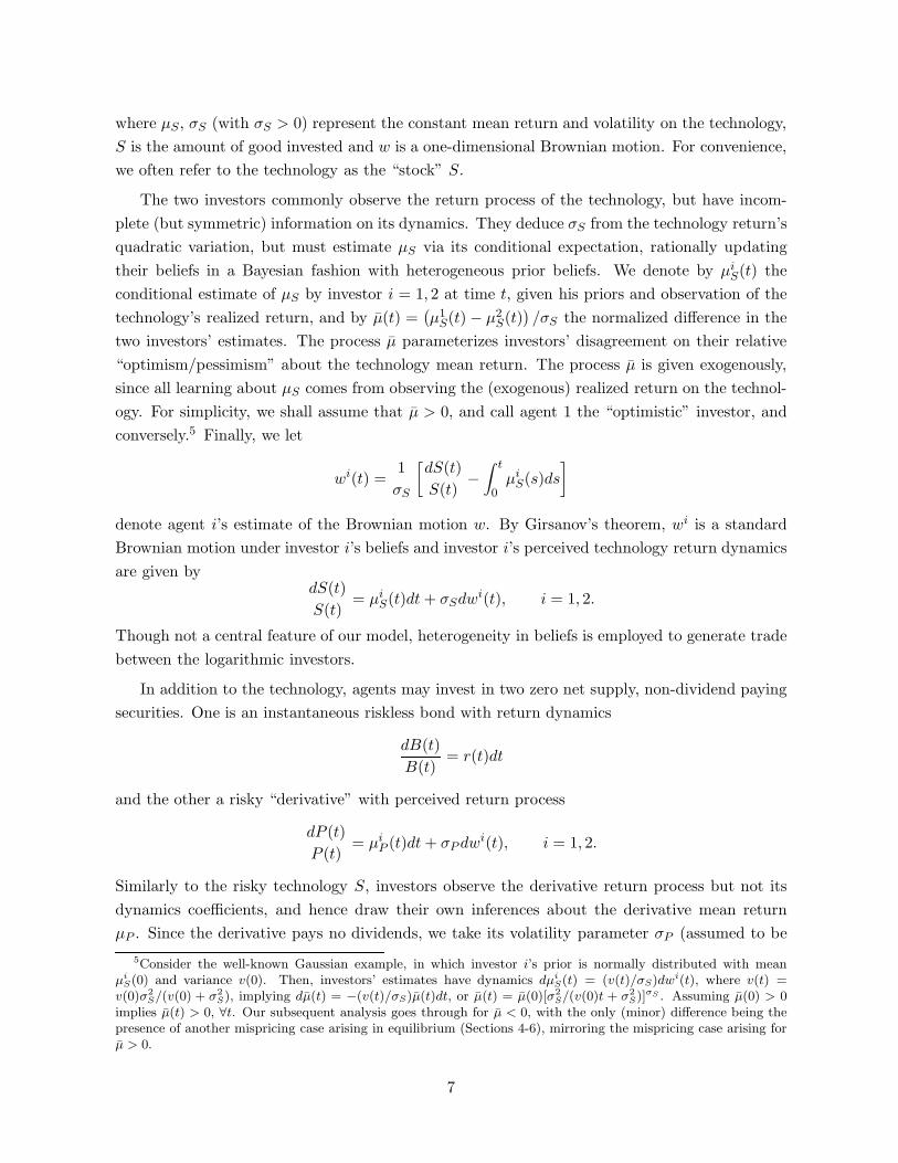
where µS, σS (with σS > 0) represent the constant mean return and volatility on the technology,S is the amount of good invested and w is a one-dimensional Brownian motion. For convenience,we often refer to the technology as the “stock” S.

The two investors commonly observe the return process of the technology, but have incom-plete (but symmetric) information on its dynamics. They deduce σS from the technology return’squadratic variation, but must estimate µS via its conditional expectation, rationally updatingtheir beliefs in a Bayesian fashion with heterogeneous prior beliefs. We denote by µi

S(t) theconditional estimate of µS by investor i = 1, 2 at time t, given his priors and observation of thetechnology’s realized return, and by µ(t) =

(µ1

S(t) − µ2S(t)

)/σS the normalized difference in the

two investors’ estimates. The process µ parameterizes investors’ disagreement on their relative“optimism/pessimism” about the technology mean return. The process µ is given exogenously,since all learning about µS comes from observing the (exogenous) realized return on the technol-ogy. For simplicity, we shall assume that µ > 0, and call agent 1 the “optimistic” investor, andconversely.5 Finally, we let

wi(t) =1σS

[dS(t)S(t)

−∫ t

0µi

S(s)ds

]

denote agent i’s estimate of the Brownian motion w. By Girsanov’s theorem, wi is a standardBrownian motion under investor i’s beliefs and investor i’s perceived technology return dynamicsare given by

dS(t)S(t)

= µiS(t)dt + σSdwi(t), i = 1, 2.

Though not a central feature of our model, heterogeneity in beliefs is employed to generate tradebetween the logarithmic investors.

In addition to the technology, agents may invest in two zero net supply, non-dividend payingsecurities. One is an instantaneous riskless bond with return dynamics

dB(t)B(t)

= r(t)dt

and the other a risky “derivative” with perceived return process

dP (t)P (t)

= µiP (t)dt + σP dwi(t), i = 1, 2.

Similarly to the risky technology S, investors observe the derivative return process but not itsdynamics coefficients, and hence draw their own inferences about the derivative mean returnµP . Since the derivative pays no dividends, we take its volatility parameter σP (assumed to be

5Consider the well-known Gaussian example, in which investor i’s prior is normally distributed with meanµi

S(0) and variance v(0). Then, investors’ estimates have dynamics dµiS(t) = (v(t)/σS)dwi(t), where v(t) =

v(0)σ2S/(v(0) + σ2

S), implying dµ(t) = −(v(t)/σS)µ(t)dt, or µ(t) = µ(0)[σ2S/(v(0)t + σ2

S)]σS . Assuming µ(0) > 0implies µ(t) > 0, ∀t. Our subsequent analysis goes through for µ < 0, with the only (minor) difference being thepresence of another mispricing case arising in equilibrium (Sections 4-6), mirroring the mispricing case arising forµ > 0.

7

positive for simplicity) to define the derivative contract P , as is standard in the literature (e.g.,Karatzas and Shreve (1998)). Any security whose price is continuously resettled (e.g., a futurescontract) is an example of this derivative.6 The other security return parameters, the interestrate r and the perceived mean returns µi

P , are to be determined endogenously in equilibrium.

3.2. Investors’ Optimization problems

With all the uncertainty generated by a one-dimensional Brownian motion, the technology andderivative returns are perfectly correlated, and so the derivative is redundant. However, positionlimits on investors’ risky investments generate an economic role for the derivative. Lettingθi ≡

(θiB, θi

S , θiP

), with θi

B = W i(t)−θiS(t)−θi

P (t), denote the amounts of investor i’s wealth, W i,invested in B, S and P respectively, we assume that, in addition to short sales being prohibited,investments in the technology are bounded from above, and that investments in the derivativeare bounded from below at all times:

0 ≤ θiS(t) ≤ βW i(t), θi

P (t) ≥ −γW i(t), (3.1)

where β ≥ 1, γ > 0.7

Absent position limits, with one factor of risk no-arbitrage would enforce identical marketprices of risk across the risky assets. This motivates our definition of mispricing between thetechnology and derivative under an investor i’s beliefs as the difference between their marketprices of risk:

∆iS,P (t) ≡ µi

S(t) − r(t)σS

− µiP (t) − r(t)

σP.

We note that the observed return agreement across investors enforces agreement on the mispric-ing: ∆1

S,P (t) = ∆2S,P (t) ≡ ∆S,P (t). We say that S is favorable if ∆S,P (t) > 0, and conversely.

The investor i is endowed with initial wealth W i(0). He then chooses a consumption policyci and investment strategy θi so as to maximize his expected lifetime logarithmic utility subjectto the dynamic budget constraint and position limits, that is to solve the problem:

maxci,θi Ei[∫ T

0 log(ci(t)

)dt

]

s. t. dW i(t) =[W i(t)r(t) − ci(t)

]dt +

{θiS(t)

[µi

S(t) − r(t)]+ θi

P (t)[µi

P (t) − r(t)]}

dt

+[θiS(t)σS + θi

P (t)σP]dwi(t)

and (3.1)

This differs from the standard frictionless investor’s dynamic optimization problem due to theposition limits, potential redundancy and mispricing between the risky assets S and P . The

6Defining P by its dividend process δP would not entail major changes to our analysis. All of the expressions inthe paper would remain valid, but σP would be endogenously determined, via a present value formula. Our mainpoints and intuition would be unaffected.

7Assuming more constraints for the investors (for example, a lower bound on holdings of the derivative) wouldonly complicate the model without substantially affecting our analysis, with extra equilibrium cases where noarbitrage activity takes place.

8

solution of the investor i’s problem is reported in Proposition 3.1. Those cases where P isfavorable are ignored, as they cannot arise in equilibrium.

Proposition 3.1. Investor i’s optimal consumption and investments in the technology S andderivative P are given by:

ci(t) =W i(t)T − t

;

when there is no mispricing,

θiS(t)

W i(t)=

∈[0, β

],

0,

θiP (t)

W i(t)=

≥ −γσP , s.t. σSθiS(t)

W i(t)+ σP

θiP (t)

W i(t)= µi

S(t)−r(t)σS

, (a)

if µiS(t)−r(t)

σS= µi

P (t)−r(t)σP

≥ −γσP ,

−γ if µiS(t)−r(t)

σS= µi

P (t)−r(t)σP

< −γσP , (b)

and when there is mispricing with S being more favorable,

θiS(t)

W i(t)=

β if µiS(t)−r(t)

σS>

µiP (t)−r(t)

σP≥ −γσP + βσS , (c)

β if µiS(t)−r(t)

σS> −γσP + βσS >

µiP (t)−r(t)

σP, (d)

µiS(t)−r(t)

σ2S

+ γ σPσS

if − γσP + βσS ≥ µiS(t)−r(t)

σS

{≥ −γσP ,

>µi

P (t)−r(t)σP

,(e)

0 if − γσP >µi

S(t)−r(t)σS

>µi

P (t)−r(t)σP

. (f)

θiP (t)

W i(t)=

µiP (t)−r(t)

σ2P

− β σSσP

if (c)

−γ if (d)

−γ if (e)

−γ if (f)

An investor can be in one of six possible scenarios, (a)-(f), depending on the economic envi-ronment and whether there is mispricing (cases (c)-(f)) or not (cases (a)-(b)). When there is nomispricing and the perceived market price of risk is low enough, the investor binds on his lowerposition limit of both risky assets (case (b)), otherwise he is indifferent between the same riskyassets provided his position is feasible (case (a)).

Under mispricing, the investor takes on as much of a riskless, costless arbitrage position asallowed by the position limits, hence uniquely determining the allocation between the derivativeand the technology. When the risky technology is favorably mispriced and the investor is rela-tively optimistic about both S and P (case (c)), he desires a high risk exposure, wishing to golong in both risky assets, and so ends up binding on the upper position limit of S. Otherwise, hisrelative pessimism about the derivative drives him to his position limit on P ; when additionallypessimistic about S, he desires a low risk exposure and so does not invest in the technology (case(f)), otherwise he goes long in the technology (cases (d)-(e)). As will be demonstrated in Section4.2, mispricing cases (c) and (e) may occur in equilibrium (with or without an arbitrageur).Cases (d) and (f) do not.

9

4. Equilibrium with a Competitive Arbitrageur

4.1. The Arbitrageur

We assume that, in addition to the two investors i = 1, 2, the economy is populated by anarbitrageur indexed by i = 3. The arbitrageur is assumed to take on only riskless, costlessarbitrage positions, and to maximize his expected cumulated profits under a limit on the sizeof his positions. Denoting his (dollar) investments by θ3 ≡

(θ3B, θ3

S , θ3P

), his problem can be

expressed as follows:

maxθ3

E3

[∫ T

0Ψ3(t)dt

]

s.t. Ψ3(t)dt ={θ3S(t)µ3

S(t) + θ3P (t)µ3

P (t) + θ3B(t)r(t)

}dt

+[θ3S(t)σS + θ3

P (t)σP ]dw3(t)

θ3S(t) + θ3

P (t) + θ3B(t) = 0 (4.1)

θ3S(t)σS + θ3

P (t)σP = 0 (4.2)

0 ≤ θ3S(t) ≤ M (4.3)

Conditions (4.1)-(4.2) imply:

θ3P (t) = −σS

σPθ3S(t), θ3

B(t) =(

σS

σP− 1

)θ3S(t), (4.4)

so that the arbitrageur’s holdings in all securities are pinned down by his stock investment.Therefore, the constraint on holdings of the stock (4.3) also limits the arbitrageur’s holdings ofthe other securities.

In the absence of mispricing (∆S,P = 0), it is straightforward to verify that the arbitrageur isindifferent between all portfolio holdings that satisfy (4.3)-(4.4), since they all provide him withzero cash-flows (and he can do no better than this). In the presence of mispricing (∆S,P > 0),however, as long as θ3

S > 0 the arbitrageur receives a profit that is proportional to θ3S. The

optimal policy is then to choose the maximal possible value for θ3S , namely M . From (4.4), the

other holdings are given by θ3P (t) = −MσS/σP and θ3

B(t) = M (σS/σP − 1), and the arbitrageur’sinstantaneous profit rate by:

Ψ3(t) = θ3S(t)µ3

S(t) + θ3P (t)µ3

P (t) + θ3B(t)r(t) = MσS∆S,P (t).

It should be pointed that the (price-taking) arbitrageur’s solution (as well as the value of hisprofits) is independent of his beliefs and preferences. Due to his constraints, (4.1)-(4.2), thearbitrageur consumes his profits as they are made (c3 = Ψ3) and hold no net wealth, so thathe can be assumed to be risk-neutral, without any time-preference, without loss of generality.Any increasing utility function for the arbitrageur would lead to the same behavior as for therisk-neutral arbitrageur, in this Section as well as Sections 5 and 6.

10

4.2. Analysis of Equilibrium

Definition 4.1 (Competitive Equilibrium). An equilibrium is a price system (r, µ1P , µ2

P ) andconsumption-portfolio processes (ci, θi) such that: (i) agents choose their optimal consumption-portfolio strategies given their beliefs; (ii) security markets clear, i.e.,

θ1P (t) + θ2

P (t) + θ3P (t) = 0, θ1

B(t) + θ2B(t) + θ3

B(t) = 0. (4.5)

We now proceed to the characterization of equilibrium. Quantities of interest will be expressedas a function of two (endogenous) state variables: the aggregate wealth W ≡ W 1+W 2 (coinciding,in equilibrium, with the total amount invested in the production technology), and the proportionof aggregate wealth held by investor 1, λ ≡ W 1/W . Several cases are possible in equilibrium,depending on investor 1 and 2’s binding constraints. We denote each one by the optimizationcase in which each of investors 1 and 2 is. For example, in equilibrium (a,a) each investor is incase a, in equilibrium (a,b) investor 1 is in case a and investor 2 in case b, etc..

Proposition 4.1 reports the possible equilibrium cases, the conditions for their occurrence,and characterizes economic quantities (prices and consumptions) in each case.

Proposition 4.1. If equilibrium exists, the investors’ optimization cases, equilibrium mispricingand interest rate, and distribution of wealth dynamics are as follows.

When µ(t) ≤γσP

λ(t)+ σS min

{1

λ(t),

11 − λ(t)

[(β − 1

)+

M

λ(t)W (t)

]},

agents are in (a,a) and

∆S,P (t) = 0 and r(t) = λ(t)µ1S(t) + (1 − λ(t))µ2

S(t) − σ2S ,

dλ(t) = λ(t)(1 − λ(t))2 (µ(t))2 dt + λ(t)(1 − λ(t))µ(t)dw1(t). (4.6)

When µ(t) >γσP + σS

λ(t)and λ(t) ≥ 1

β

(1 − M

W (t)

),

agents are in (a,b) and

∆S,P (t) = 0 and r(t) = µ1S(t) − σ2

S −(

1λ(t)

− 1)

σS (σS + γσP ) ,

dλ(t) =(1 − λ(t))2

λ(t)

(σS + γσP

)dt + (1 − λ(t))

(σS + γσP

)dw1(t).

When µ(t) >γσP

λ(t)+

σS

1 − λ(t)

[(β − 1

)+

M

λ(t)W (t)

]and λ(t) <

1β

(1 − M

W (t)

)(4.7)

agents are in (c,e) and

∆S,P (t) = µ(t) −σS

(β − 1

)

1 − λ(t)−

γσP

λ(t)− σSM

λ(t)(1 − λ(t))W (t)> 0,

11

r(t) = µ2S(t) − σ2

S + γσSσP + σ2S

[(β − 1

) λ(t)1 − λ(t)

+M

(1 − λ(t))W (t)

],

dλ(t) = λ(t){

σS∆S,P (t)[(

β − 1)

+M

W (t)

]+ [(1 − λ(t)) (µ(t) − ∆S,P (t))]2

}dt

+λ(t)(1 − λ(t)) (µ(t) − ∆S,P (t)) dw1(t). (4.8)

In all cases, the aggregate wealth dynamics follow

dW (t) =[W (t)

(µ1

S(t) − 1T − t

)− MσS∆S,P (t)

]dt + W (t)σSdw1(t) (4.9)

and investors 1 and 2’s consumption and the arbitrageur’s profit are given by:

c1(t) =λ(t)W (t)

T − t, c2(t) =

(1 − λ(t))W (t)T − t

, Ψ3(t) = MσS∆S,P (t).

Three cases are possible in equilibrium: (a,a) and (a,b) where there is no mispricing andthe arbitrageur makes no profits, and (c,e) where mispricing occurs. In (a,a), there is onlymoderate divergence in beliefs across investors and so no constraints are binding. Heterogeneityis not sufficient for the investors to deviate very much from the no-trade case (where both ofthem would invest all of their wealth in the technology) and hit the constraints. Accordingly,the economic quantities are as in an unconstrained economy. When heterogeneity in beliefs ishigh enough, investors find it optimal to trade more, and some constraints are binding (regions(a,b) and (c,e)). The equilibrium with mispricing (c,e) occurs when the more optimistic investor(1) is insufficiently wealthy relative to the pessimistic investor (2) (low λ). Then, absent themispricing the pessimistic investor would only invest a small amount in the technology and, dueto his upper bound on investments in the technology, the optimistic investor would be unable toinvest enough for market clearing to obtain (which requires that the whole aggregate wealth beinvested in the technology: combining both clearing conditions in the definition of equilibrium((4.5)) yields: θ1

S + θ2S = W ). The mispricing, with S being favorably mispriced, increases

investor 2’s demand therein and so allows for market clearing. The intuition for the occurrenceof mispricing is elaborated on further in Basak and Croitoru (2000). When, in contrast, agent 1is sufficiently wealthy, it is possible for him to invest enough in the technology without violatinghis upper bound, and so it is not necessary to increase agent 2’s investment, and equilibrium(a,b) (without mispricing) obtains.

We henceforth concentrate on region (c,e), where the arbitrageur has an economic impact andso affects the characterization of economic quantities. In region (a,a), the equilibrium is as in anunconstrained economy as analyzed by Detemple and Murthy (1994), and in region (a,b), theequilibrium is similar to a constrained economy without a derivative as in Detemple and Murthy(1997). In both of these cases, there is no arbitrage available. It is straightforward to check thatregion (c,e) does occur for plausible parameter values: for example, according to (4.7), if γ = 0.5,β = 1.5, σS = σP = 0.1, M/W (t) = 0.1, λ(t) = 0.5, region (c,e) occurs whenever investor 1’sestimate of the mean instantaneous return of the technology exceeds investor 2’s estimate by

12

at least 2.4% per year. In our analysis of economic quantities, we focus on the terms reflectingthe effects of the arbitrageur’s presence and the size of his position (measured by M). All ofour analyses and comparisons are valid only for given aggregate wealth (W ) and distribution ofwealth (λ). For comparison with our economy, we introduce the following benchmarks:

Economy I : no constraints, no derivative, otherwise as our economy;

Economy II : no arbitrageur, otherwise as our economy.In Economy I, all equilibrium quantities are as in our region (a,a), while in Economy II, they areas in our economy, for the particular case where M = 0.

The value of the mispricing can be interpreted as the amount of heterogeneity (in beliefs) thatinvestors cannot trade on, due to the binding constraints. On moving from region (a,a) to region(c,e), the mispricing starts at a value of zero and then increases linearly with heterogeneity (µ)while inter-agent transfers remain stuck due to the constraints. The mispricing is decreased by thepresence of the arbitrageur, and decreases further as the size of his position increases; comparingwith our benchmarks, we have: ∆I

S,P = 0 < ∆S,P < ∆IIS,P . Keeping in mind our interpretation of

the mispricing as the amount of un-traded heterogeneity, this suggests an improvement in risk-sharing due to the arbitrageur’s presence. The size of the arbitrageur’s position only matters viaits ratio to aggregate wealth, because what matters is the size of the counterparty he can offer tothe investors, relative to their own wealths. This generates a dependence of the mispricing withrespect to aggregate wealth: the higher aggregate wealth is, the less important the arbitrageur isrelative to the other agents and so the less valuable the improvement in risk-sharing he generates.This increases the value of the mispricing and the arbitrageur’s profits, which are thus shown tobe procyclical.

The value of the interest rate is increased by the presence of the arbitrageur; we have: rI >

r > rII . This is also indirect evidence of an improvement in risk-sharing between investors dueto the arbitrageur’s presence: improved risk-sharing decreases investors’ precautionary savings.For the bond market to clear in spite of this, it is necessary for the interest rate to rise, thusbecoming closer to its value in an unconstrained economy.

In short, the impact of the arbitrageur on all price dynamics parameters is to make them closerto their values in an unconstrained economy; the larger his position, the closer the equilibriumto an unconstrained one. The conditions for region (c,e) to occur (and the constraints to bind)are also affected. From (4.7), it is clear that the larger the arbitrageur’s position, the less likelyregion (c,e) is to occur and the constraints are to bind, perturbing risk-sharing between investors.In all cases, the effect of increasing the size of the arbitrageur’s position (M) on the expressionsis tantamount to an increase in β or γ (i.e., an alleviation of the constraints.)

All of this suggests that the arbitrageur alleviates the effect of the portfolio constraints. Theeffect of his presence on the investors’ welfare is ambiguous, however, because his profits reducethe growth of the investors’ aggregate wealth ((4.9)).

13

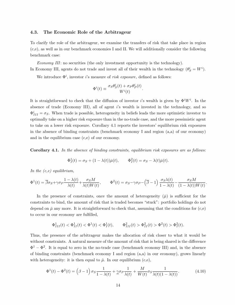
4.3. The Economic Role of the Arbitrageur

To clarify the role of the arbitrageur, we examine the transfers of risk that take place in region(c,e), as well as in our benchmark economies I and II. We will additionally consider the followingbenchmark case:

Economy III : no securities (the only investment opportunity is the technology).In Economy III, agents do not trade and invest all of their wealth in the technology (θi

S = W i).

We introduce Φi, investor i’s measure of risk exposure, defined as follows:

Φi(t) ≡ σSθiS(t) + σP θi

P (t)W i(t)

.

It is straightforward to check that the diffusion of investor i’s wealth is given by ΦiW i. In theabsence of trade (Economy III), all of agent i’s wealth is invested in the technology, and soΦi

III = σS . When trade is possible, heterogeneity in beliefs leads the more optimistic investor tooptimally take on a higher risk exposure than in the no-trade case, and the more pessimistic agentto take on a lower risk exposure. Corollary 4.1 reports the investors’ equilibrium risk exposuresin the absence of binding constraints (benchmark economy I and region (a,a) of our economy)and in the equilibrium case (c,e) of our economy.

Corollary 4.1. In the absence of binding constraints, equilibrium risk exposures are as follows:

Φ1I(t) = σS + (1 − λ(t))µ(t), Φ2

I(t) = σS − λ(t)µ(t).

In the (c,e) equilibrium,

Φ1(t) = βσS+γσP1 − λ(t)

λ(t)+

σSM

λ(t)W (t), Φ2(t) = σS−γσP−

(β − 1

) σSλ(t)1 − λ(t)

− σSM

(1 − λ(t))W (t).

In the presence of constraints, once the amount of heterogeneity (µ) is sufficient for theconstraints to bind, the amount of risk that is traded becomes “stuck”: portfolio holdings do notdepend on µ any more. It is straightforward to check that, assuming that the conditions for (c,e)to occur in our economy are fulfilled,

Φ1III(t) < Φ1

II(t) < Φ1(t) < Φ1I(t), Φ2

III(t) > Φ2II(t) > Φ2(t) > Φ2

I(t).

Thus, the presence of the arbitrageur makes the allocation of risk closer to what it would bewithout constraints. A natural measure of the amount of risk that is being shared is the differenceΦ1 − Φ2. It is equal to zero in the no-trade case (benchmark economy III) and, in the absenceof binding constraints (benchmark economy I and region (a,a) in our economy), grows linearlywith heterogeneity: it is then equal to µ. In our equilibrium (c,e),

Φ1(t) − Φ2(t) =(β − 1

)σS

11 − λ(t)

+ γσP1

λ(t)+

M

W (t)σS

1λ(t)(1 − λ(t))

. (4.10)

14

revealing how the amount of risk that is shared between the investors grows with the size ofthe arbitrageur’s position. The mechanism through which the arbitrageur facilitates risk-sharingbetween the investors is the one already described in Section 2: the arbitrageur effectively acts asa financial intermediary who provides an additional counterparty to the investors. The analysisin Section 2 can be repeated with only insubstantial changes, provided one replaces investors’state-ω cash-flows (Ai’s) in Section 2 with their risk exposures (Φi’s). In the absence of thearbitrageur (benchmark economy II), investors’ risk exposures are:

Φ1II(t) = βσS + γσP

1 − λ(t)λ(t)

, Φ2II(t) = σS − γσP −

(β − 1

)σS

λ(t)1 − λ(t)

.

Even though the optimistic investor 1 would optimally increase his risk exposure (to Φ1I) by

increasing his holding of the derivative (since he already is binding on the technology), this isimpossible because investor 2 would then, due to his lower constraint on P , not be able to providea counterparty. By shorting the derivative, the arbitrageur provides an extra counterparty, whichallows for an increase in Φ1 (by σSM/λW ) that is proportional to the arbitrageur’s position limitM . Similarly, it is impossible for the pessimistic investor 2 to invest as little in the stock as heoptimally would, because then clearing in the bond market (which requires θ1

S + θ2S = W ) would

not obtain. By investing in the stock, the arbitrageur makes it possible for the pessimistic investorto hold less of it and so reduce his risk exposure (by σSM/[(1 − λ)W ]). The introduction of thearbitrageur in the economy is equivalent to that of an extra, zero-net supply security, in whichboth investors face a position limit proportional to M . This security is being purchased from thepessimistic investor by the innovator, the arbitrageur, and resold to the optimistic investor at ahigher price. The difference (the mispricing) generates the arbitrageur’s profit.

Our understanding of the role of the arbitrageur allows us to provide additional insight onsome of the characterizations in Proposition 4.1. The distribution of wealth (λ) dynamics isaffected by the presence of the arbitrageur. When no constraints are binding, the volatility ofinvestor 1’s share of aggregate wealth is given by λ(1 − λ)µ (from equation (4.6)): the moreoptimistic investor 1 is (i.e., the higher µ), the more positively his wealth covaries with thetechnology return. In region (c,e) of our constrained economy, due to the binding constraintsinvestors cannot trade as much risk as in the unconstrained case and accordingly the volatility ofλ is reduced to λ(1 − λ) (µ − ∆S,P ) (from (4.8)). In the presence of an arbitrageur, the value ofthe mispricing is reduced; this increases the covariance of investor 1’s wealth with the technologyreturn, thanks to improved risk-sharing.

Finally, we note that much of the above analysis is not dependent on the logarithmic utilityassumption. The investors’ portfolio holdings in region (c,e) follow directly from the bindingposition limits and the market clearing conditions. Thus, whenever mispricing occurs, theseholdings obtain for arbitrary investor preferences or beliefs, and our analysis of the arbitrageur’scontribution to improved risk-sharing is equally valid. Only the occurrence of mispricing is neededfor this. Basak and Croitoru (2000, Proposition 5) show how and when mispricing may arise inequilibrium under very general assumptions, demonstrating the robustness of our analysis.

15

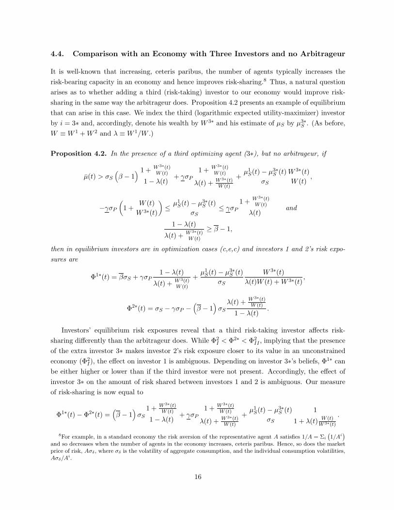
4.4. Comparison with an Economy with Three Investors and no Arbitrageur

It is well-known that increasing, ceteris paribus, the number of agents typically increases therisk-bearing capacity in an economy and hence improves risk-sharing.8 Thus, a natural questionarises as to whether adding a third (risk-taking) investor to our economy would improve risk-sharing in the same way the arbitrageur does. Proposition 4.2 presents an example of equilibriumthat can arise in this case. We index the third (logarithmic expected utility-maximizer) investorby i = 3∗ and, accordingly, denote his wealth by W 3∗ and his estimate of µS by µ3∗

S . (As before,W ≡ W 1 + W 2 and λ ≡ W 1/W .)

Proposition 4.2. In the presence of a third optimizing agent (3∗), but no arbitrageur, if

µ(t) > σS

(β − 1

) 1 + W 3∗(t)W (t)

1 − λ(t)+ γσP

1 + W 3∗(t)W (t)

λ(t) + W 3∗(t)W (t)

+µ1

S(t) − µ3∗S (t)

σS

W 3∗(t)W (t)

,

−γσP

(1 +

W (t)W 3∗(t)

)≤ µ1

S(t) − µ3∗S (t)

σS≤ γσP

1 + W 3∗(t)W (t)

λ(t)and

1 − λ(t)

λ(t) + W 3∗(t)W (t)

≥ β − 1,

then in equilibrium investors are in optimization cases (c,e,c) and investors 1 and 2’s risk expo-sures are

Φ1∗(t) = βσS + γσP1 − λ(t)

λ(t) + W 3(t)W (t)

+µ1

S(t) − µ3∗S (t)

σS

W 3∗(t)λ(t)W (t) + W 3∗(t)

,

Φ2∗(t) = σS − γσP −(β − 1

)σS

λ(t) + W 3∗(t)W (t)

1 − λ(t).

Investors’ equilibrium risk exposures reveal that a third risk-taking investor affects risk-sharing differently than the arbitrageur does. While Φ2

I < Φ2∗ < Φ2II , implying that the presence

of the extra investor 3∗ makes investor 2’s risk exposure closer to its value in an unconstrainedeconomy (Φ2

I), the effect on investor 1 is ambiguous. Depending on investor 3∗’s beliefs, Φ1∗ canbe either higher or lower than if the third investor were not present. Accordingly, the effect ofinvestor 3∗ on the amount of risk shared between investors 1 and 2 is ambiguous. Our measureof risk-sharing is now equal to

Φ1∗(t) − Φ2∗(t) =(β − 1

)σS

1 + W 3∗(t)W (t)

1 − λ(t)+ γσP

1 + W 3∗(t)W (t)

λ(t) + W 3∗(t)W (t)

+µ1

S(t) − µ3∗S (t)

σS

1

1 + λ(t) W (t)W 3∗(t)

.

8For example, in a standard economy the risk aversion of the representative agent A satisfies 1/A = Σi

(1/Ai

)and so decreases when the number of agents in the economy increases, ceteris paribus. Hence, so does the marketprice of risk, Aσδ, where σδ is the volatility of aggregate consumption, and the individual consumption volatilities,Aσδ/A

i.

16

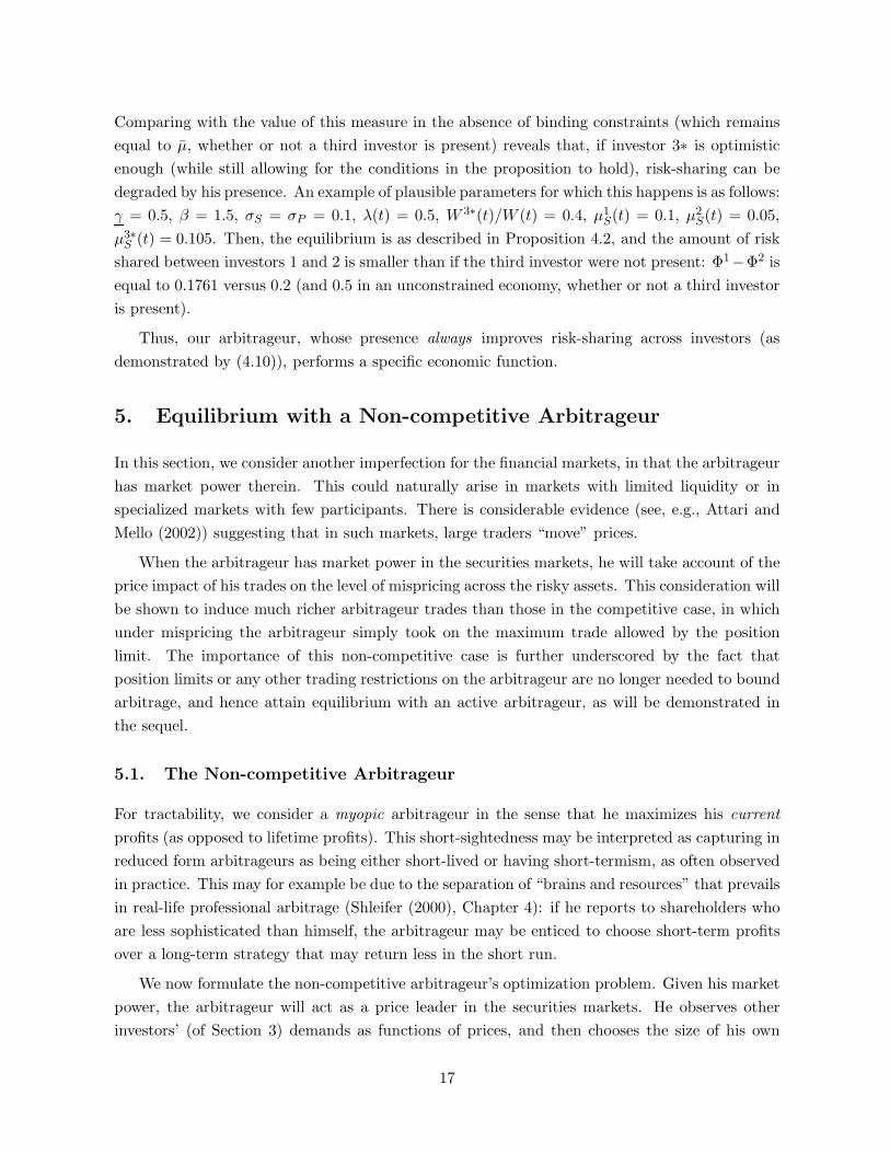
Comparing with the value of this measure in the absence of binding constraints (which remainsequal to µ, whether or not a third investor is present) reveals that, if investor 3∗ is optimisticenough (while still allowing for the conditions in the proposition to hold), risk-sharing can bedegraded by his presence. An example of plausible parameters for which this happens is as follows:γ = 0.5, β = 1.5, σS = σP = 0.1, λ(t) = 0.5, W 3∗(t)/W (t) = 0.4, µ1

S(t) = 0.1, µ2S(t) = 0.05,

µ3∗S (t) = 0.105. Then, the equilibrium is as described in Proposition 4.2, and the amount of risk

shared between investors 1 and 2 is smaller than if the third investor were not present: Φ1−Φ2 isequal to 0.1761 versus 0.2 (and 0.5 in an unconstrained economy, whether or not a third investoris present).

Thus, our arbitrageur, whose presence always improves risk-sharing across investors (asdemonstrated by (4.10)), performs a specific economic function.

5. Equilibrium with a Non-competitive Arbitrageur

In this section, we consider another imperfection for the financial markets, in that the arbitrageurhas market power therein. This could naturally arise in markets with limited liquidity or inspecialized markets with few participants. There is considerable evidence (see, e.g., Attari andMello (2002)) suggesting that in such markets, large traders “move” prices.

When the arbitrageur has market power in the securities markets, he will take account of theprice impact of his trades on the level of mispricing across the risky assets. This consideration willbe shown to induce much richer arbitrageur trades than those in the competitive case, in whichunder mispricing the arbitrageur simply took on the maximum trade allowed by the positionlimit. The importance of this non-competitive case is further underscored by the fact thatposition limits or any other trading restrictions on the arbitrageur are no longer needed to boundarbitrage, and hence attain equilibrium with an active arbitrageur, as will be demonstrated inthe sequel.

5.1. The Non-competitive Arbitrageur

For tractability, we consider a myopic arbitrageur in the sense that he maximizes his currentprofits (as opposed to lifetime profits). This short-sightedness may be interpreted as capturing inreduced form arbitrageurs as being either short-lived or having short-termism, as often observedin practice. This may for example be due to the separation of “brains and resources” that prevailsin real-life professional arbitrage (Shleifer (2000), Chapter 4): if he reports to shareholders whoare less sophisticated than himself, the arbitrageur may be enticed to choose short-term profitsover a long-term strategy that may return less in the short run.

We now formulate the non-competitive arbitrageur’s optimization problem. Given his marketpower, the arbitrageur will act as a price leader in the securities markets. He observes otherinvestors’ (of Section 3) demands as functions of prices, and then chooses the size of his own

17

trades so as to maximize his concurrent profits subject to the condition that the security marketsclear. Of course, he will only be active when there is mispricing and hence positive profits;otherwise his profits are zero. Accordingly, given the investors’ optimal investments (Proposition3.1), clearing in the security markets implies the following when mispricing (case (c,e)) occurs:

∆S,P (t) = µ(t) −σS

(β − 1

)

1 − λ(t)−

γσP

λ(t)− σSθ3

S(t)λ(t)(1 − λ(t))W (t)

. (5.1)

Hence, the arbitrageur’s influence on security prices manifests itself, via (5.1), as the size of hisstock position affecting mispricing, The larger his position is, the lower the mispricing – in asense, the prices move against him: the value of his marginal profit (the mispricing) is reducedby his trades.

The non-competitive arbitrageur solves the following optimization problem at time t:

maxθ3S(t),∆S,P (t)

Ψ3(t) = θ3S(t)σS∆S,P (t) (5.2)

s.t. θ3S(t) + θ3

P (t) + θ3B(t) = 0, θ3

S(t)σS + θ3P (t)σP = 0, ((4.1)-(4.2))

and ∆S,P (t) satisfies (5.1).

As for the competitive arbitrageur, the costless-riskless arbitrage conditions, (4.1)-(4.2), uniquelydetermine the non-competitive arbitrageur’s holdings in financial securities in terms of his stockinvestment. Finally, we note that the maximization problem (5.2) is a simple concave quadraticproblem.

5.2. Analysis of Equilibrium

Definition 5.1 (Non-competitive Equilibrium). Equilibrium in an economy with two risk-averse investors and one non-competitive arbitrageur is a price system (r, µ1

P , µ2P ) and consumption-

portfolio policies (ci, θi) such that: (i) investors choose their optimal policies given the price sys-tem (r, µ1

P , µ2P ) and their beliefs; (ii) the arbitrageur chooses his optimal trades in (5.2) taking

into account that the mispricing responds to clear the security markets; (iii) the price system issuch that all the security markets clear.

According to the definition of a non-competitive equilibrium, the non-competitive arbitrageursimultaneously solves for the optimal size of his arbitrage trades and the equilibrium mispricing.Proposition 5.1 reports the possible equilibrium cases and the characterization for each case.

18

Proposition 5.1. If equilibrium exists, equilibrium with a non-competitive arbitrageur is as fol-lows.

When µ(t) ≤ γσP

λ(t) + σS min{

1λ(t) ,

β−11−λ(t)

}, agents are in (a,a), and when µ(t) >

γσP +σS

λ(t) andλ(t) ≥ 1

β, agents are in (a,b). In both cases, ∆S,P (t), r(t) and λ(t) are as in the competitive

arbitrageur equilibrium described in Proposition 4.1.

When µ(t) >γσP

λ(t) +σS(β−1)1−λ(t) and λ(t) < 1

β, investors are in (c,e) and the arbitrageur’s equilibrium

stock investment and profit are given by

θ3S(t) =

λ(t)(1 − λ(t))W (t)2σS

µ(t) −

σS

(β − 1

)

1 − λ(t)− γσP

λ(t)

, (5.3)

Ψ3(t) =λ(t)(1 − λ(t))W (t)

4

µ(t) −

σS

(β − 1

)

1 − λ(t)− γσP

λ(t)

2

,

and the equilibrium mispricing, interest rate and distribution of wealth dynamics are given by

∆S,P (t) =12

µ(t) −

σS

(β − 1

)

1 − λ(t)−

γσP

λ(t)

,

r(t) = µ2S(t) − σ2

S + σSµ(t)λ(t)2

+12γσSσP +

12

λ(t)1 − λ(t)

σ2S

(β − 1

),

dλ(t) = λ(t)

{σS∆S,P (t)

[(β − 1

)+

θ3S(t)

W (t)

]+ [(1 − λ(t)) (µ(t) − ∆S,P (t))]2

}dt

+λ(t)(1 − λ(t)) (µ(t) − ∆S,P (t)) dw1(t).

In all cases, the aggregate wealth dynamics follow

dW (t) =[W (t)

(µ1

S(t) − 1T − t

)− θ3

S(t)σS∆S,P (t)]dt + W (t)σSdw1(t).

As in the competitive case, three cases are possible in equilibrium, with case (c,e) being themispricing case. Comparison with the competitive equilibrium of Proposition 4.1 reveals thatthe region of mispricing is larger in the non-competitive equilibrium. Hence, the presence ofthe non-competitive arbitrageur makes mispricing more likely to occur in equilibrium. This isintuitive: in the presence of mispricing, the competitive arbitrageur always trades to the fullextent that is allowed by the position limit, and so is more likely to fully “arbitrage away” themispricing, making it disappear. In the non-competitive case, in contrast, he limits his tradesso as to make the mispricing (and positive arbitrage profits) subsist under a broader range ofconditions.9 As a result, unlike in the competitive case, the conditions for regions (c,e) are as ifthe arbitrageur were not present.

9It is impossible for the arbitrageur to make the mispricing case more likely because, whenever he trades, heimproves risk-sharing across investors and reduces the mispricing.

19

As compared with the no-arbitrageur economy (Economy II, Proposition 4.1 with M = 0),we see that the equilibrium mispricing is reduced by a half, ∆S,P (t) = 1

2∆IIS,P (t). That is, instead

of providing a perfect counterparty to the two investors (which would eliminate the mispricing),when the arbitrageur is a non-price-taker, he provides only one half of that counterparty. This isalso easy to understand: the arbitrageur’s profit is proportional to the product of the mispricingand the size of his position. The mispricing is affine in θ3

S so the profit is a quadratic function ofthe arbitrageur’s position. Therefore, it is maximized at a position equidistant from zero (whichwould lead to zero profit) and a perfect counterparty to the investors (which would lead to zeromispricing, and hence zero profit).

In contrast to the constant competitive case, the non-competitive arbitrageur’s stock positionis stochastic, driven by the investors’ difference of opinion µ and the state variables W , λ. Forsufficiently low investor heterogeneity, the non-competitive arbitrageur’s stock position is lowerthan in the competitive case (θ3

S(t) < M), and higher for high investor heterogeneity. Hence,for low investor heterogeneity, the non-competitive equilibrium mispricing is higher than thecompetitive one. Consequently, the economic role of the arbitrageur (as discussed in Section 4), interms of alleviating the effect of portfolio constraints and facilitating the transfer of risk amongstinvestors, is reduced. The opposite holds when there is high heterogeneity amongst investors:the economic role of the non-competitive arbitrageur is more pronounced. Nonetheless, ourdiscussion of the economic role of the arbitrageur in Section 4 remains valid, when the exogenousposition limit M is replaced with the endogenous θ3

S . Finally, in contrast to the linear competitivecase, the non-competitive arbitrageur’s profits are convex in the extent of heterogeneity amongstinvestors.

6. Equilibrium with an Arbitrageur subject to Margin Require-ments

We now return to a competitive market, and assume that the arbitrageur is subject to marginrequirements. He then needs to be endowed with some capital, which we assume to be held (asan investment) by the investors. In addition to being more realistic, this modification of ourmodel allows us to endogenize the amount of capital that is allocated to arbitrage activity andthe size of the arbitrage positions.

6.1. The Arbitrageur under Margin Requirements

The economic setup introduced in Sections 3 and 4 is modified as follows. Riskless, costlessstorage, henceforth referred to as cash, is available to the agents in addition to the technology,derivative and bond. Assuming that r(t) > 0, the investors would never find it optimal to investin cash. However, the arbitrageur may be forced to hold cash due to his margin requirements, thatare as follows: letting θ3

C and W 3 denote the arbitrageur’s cash holding and capital, respectively,

20

his holdings must obey:

W 3(t) ≥ η max{−θ3

P (t), 0}

+ η(θS(t) + max

{θ3P (t), 0

}), (6.1)

θ3C(t) ≥

(1 + εη max

{−θ3

P (t), 0})

, (6.2)

where η, η, ε ∈ [0, 1] and θ3S(t) ≥ 0 (hence there is no need to account for short positions in S in

(6.1)-(6.2)). While equation (6.1) limits the size of the arbitrageur’s position in proportion to hiscapital, equation (6.2) states that the arbitrageur does not get the use of proceeds from his shortposition in the derivative; rather, these must be kept in cash as a deposit. In addition, a fractionε of the margin on the short sale must also be met with cash. For clarity, we will refer below to(6.1) as the “margin constraint” and to (6.2) as the “cash constraint”. Our modeling of marginrequirements is standard (see, e.g., Cuoco and Liu (2000)).10 For simplicity, we assume thatthere is no difference between initial and maintenance margin. Denoting θ3 ≡

(θ3B, θ3

S , θ3P , θ3

C

),

the arbitrageur’s problem is as follows:

maxθ3

E3

[∫ T

0Ψ3(t)dt

]

s.t. Ψ3(t)dt ={θ3S(t)µ3

S(t) + θ3P (t)µ3

P (t) + θ3B(t)r(t)

}dt

+[θ3S(t)σS + θ3

P (t)σP ]dw3(t),

θ3S(t) + θ3

P (t) + θ3B(t) + θ3

C(t) = W 3(t), (6.3)

θ3S(t)σS + θ3

P (t)σP = 0 (6.4)

and (6.1)-(6.2) hold.

Both the amount of arbitrage capital (W 3) and its time t-instantaneous return ((Ψ3(t)/W 3(t)

)dt)

are to be determined endogenously in equilibrium. Restrictions (6.3), (6.4) and equality in (6.2)(which always holds because cash is dominated by the bond) yield all holdings as a function ofθ3P (t):

θ3S(t) = −σP

σSθ3P (t), θ3

B(t) =(

σP

σS− 1

)θ3P (t) −

(1 + εη

)max

{−θ3

P (t), 0}

, (6.5)

θ3C(t) =

(1 + εη

)max

{−θ3

P (t), 0}

. (6.6)

When there is no mispricing (∆S,P (t) = 0), the arbitrageur is indifferent between all portfoliossatisfying (6.1), (6.5)-(6.6) and θ3

P (t) ≥ 0; the last inequality holds because (6.2) penalizes shortsales (the arbitrageur loses the interest on his cash deposit). As before, all feasible portfolioholdings yield zero profit. In the presence of mispricing (∆S,P (t) > 0), it is optimal for the

10Our modeling of margin requirements could easily be amended without affecting our main intuition. All thatis really needed is the presence of a constraint that limits the size of the arbitrageur’s position in proportion to hiscapital, and that of costly short sales.

21

arbitrageur to take on as large a profitable arbitrage position (long in the favorably mispricedstock, and short in the unfavorable derivative) as feasible; hence, (6.1) holds with equality:

ηθ3S(t) − ηθ3

P (t) = W 3(t),

uniquely determining the arbitrageur’s holdings as a function of his capital:

θ3P (t) = − W 3(t)

η + η σPσS

< 0, θ3S(t) =

W 3(t)η σS

σP+ η

> 0, (6.7)

θ3B(t) = W 3(t)

[1 −

εη + σPσS

η + η σPσS

], θ3

C(t) =

(1 + εη

)W 3(t)

η + η σPσS

. (6.8)

Thus, the instantaneous return on the arbitrageur’s capital is as follows:

Ψ3(t)W 3(t)

= r(t) +[σP ∆S,P (t) − r(t)

(1 + εη

)] 1η + η σP

σS

. (6.9)

6.2. Analysis of Equilibrium

The arbitrageur, in this economic setting, is interpreted as an arbitrage firm, whose stock is heldby the investors. In other words, arbitrage is another investment opportunity. Denoting by θi

A

investor i’s (dollar) investment in the arbitrage firm, his dynamic budget constraint is now:

dW i(t) =[W i(t)r(t) − ci(t)

]dt +

{θiS(t)

[µi

S(t) − r(t)]+ θi

P (t)[µi

P (t) − r(t)]}

dt

+[θiS(t)σS + θi

P (t)σP

]dwi(t) + θi

A(t)Ψ3(t)W 3(t)

dt,

while the following condition is added to the clearing conditions in the definition of equilibrium(4.5):

θ1A(t) + θ2

A(t) = W 3(t).

For simplicity, the investors’ holdings of the arbitrage firm are assumed to be unconstrained.Our assumptions from Sections 3 and 4 are otherwise unaffected. In particular, the arbitrageuris assumed to be competitive, and as before we denote W ≡ W 1 + W 2 and λ ≡ W 1/W .

In an equilibrium with mispricing, the return on arbitrage (6.9) must be consistent with thereturns on the other investment opportunities, leading to the equilibrium described by Proposi-tion 6.1.

22

Proposition 6.1. Assume that

µ(t) >γσP

λ(t)+

(β − 1

)σS

1 − λ(t)+

σSW 3(t)λ(t)(1 − λ(t))W (t)

λ(t)(1 + εη

)σS + σP

ησS + ησP

and 0 ≤ W 3(t) ≤ λ(t)W (t)

ησP + ησS

σP +(1 + εη

)σS

[1 − λ(t)

1 − λ(t)

(β − 1

)],

where

W 3(t) =σP µ(t) −

(1 + εη

)µ2

S(t) − σP σS(β−1)1−λ(t) − γσ2

P

λ(t) −(1 + εη

)σS

[σS

(1 +

λ(t)(β−1)1−λ(t)

)+ σP

]

σSησP +ησS

[(1+ε η)σS

(1−λ(t))W (t)

(2σP +

(1 + εη

)σS

)+ σ2

Pλ(t)(1−λ(t))W (t)

] .

(6.10)Then, an equilibrium where investors 1 and 2 are in cases (c,e) results, the aggregate amount ofcapital invested in arbitrage is as in equation (6.10), and the mispricing, interest rate, distributionof wealth dynamics and aggregate wealth dynamics are as follows:

∆S,P (t) = µ(t) −σS

(β − 1

)

1 − λ(t)−

γσP

λ(t)− σSW 3(t)

λ(t)(1 − λ(t))W (t)

λ(t)(1 + εη

)σS + σP

ησS + ησP

> 0, (6.11)

r(t) = µ2S(t) − σ2

S + γσSσP + σ2S

(β − 1

)λ(t)

1 − λ(t)+

W 3(t)(1 − λ(t))W (t)

σP +(1 + εη

)σS

ησP + ησS

, (6.12)

dλ(t) ={σS∆S,P (t)

(β − λ(t)

)+ (σS + σλ(t)) [σS(1 − 2λ(t)) + σλ(t)] + λ(t)σ2

S

}dt + λ(t)σλ(t)dw1(t),

where σλ(t) = (1 − λ(t)) (µ(t) − ∆S,P (t)) −W 3(t)

(1 + εη

)σ2

S

W (t)(ησS + ησP

) ,

dW (t) =

{W (t) −

(1 + εη

) [γ(1 − λ(t))W (t) +

W 3(t)η + η σP

σS

]} (µ1

S(t)dt + σSdw1(t))− W (t)

T − tdt.

Because arbitrage is riskless, equilibrium is only possible if the rate of return on arbitragecapital is equal to the riskless interest rate; otherwise, investors would face an unbounded arbi-trage opportunity and equilibrium would not obtain. From (6.9), this implies that σP ∆S,P (t) =r(t)

(1 + εη

), which leads (using (6.11) and (6.12)), to an equation affine in W 3(t), whose solu-

tion is given by (6.10). The endogenous amount of arbitrage capital W 3 is provided by equation(6.10)). Interestingly, the main factor that drives the equilibrium amount of arbitrage activityis similar to the non-competitive case of Section 5: the mispricing that would prevail withoutan arbitrageur, ∆II

S,P = µ − σS(β − 1)/(1 − λ) − γσP /λ, i.e., the amount of heterogeneity thatcannot be traded by the investors due to their constraints. This is intuitive: the higher this“un-traded” heterogeneity, the higher the profit opportunities for the arbitrageur/financial inter-mediary. As a result, the amount of arbitrage profits is convex in investor heterogeneity, as in thenon-competitive case. In addition, the amount of arbitrage capital is increasing in the severity of

23

the margin constraint (6.1) (as measured by ησP + ησS): the more stringent the constraint, thehigher the amount of capital needed to achieve a similar result. In contrast, W 3 is decreasing inthe severity of the cash constraint (6.2) (i.e., in (1 + εη)). The rationale for this will be clarifiedby our discussion on the respective impact of these two constraints on risk-sharing.

The structure of equilibrium closely resembles that of Section 4, with the exogenous positionsize M being replaced by the endogenous arbitrageur’s stock investment θ3

S = σP W 3/(ησS + ησP

).

Nonetheless, risk-sharing between investors is further impacted by the cash constraint. This isevidenced by the diffusion of the wealth distribution dynamics, σλ, which exhibits an additionalterm proportional to (1 + εη). So do the expressions for the interest rate and the mispricing,suggesting that the more severe the cash constraint, the better risk-sharing between investors.

To investigate risk-sharing among investors, we examine the investors’ risk exposures, asprovided in Proposition 6.2. We note that the expressions in the proposition are not dependentof our assumption of logarithmic utility for the investors, as they follow from the investors’binding constraints, the arbitrageur’s policy ((6.7)-(6.8)) and market clearing. (They would alsohold in a pure exchange economy.)

Proposition 6.2. In the mispriced equilibrium with an arbitrageur subject to the margin require-ment (6.1)-(6.2), the investors’ risk exposures are as follows:

Φ1(t) = βσS + γσP1 − λ(t)

λ(t)+

σSσP W 3(t)

λ(t)W (t)(ησP + ησS

) ,

Φ2(t) = σS − γσP −(β − 1

) σSλ(t)1 − λ(t)

−σS

(σP + σS

(1 + εη

))W 3(t)

(1 − λ(t))W (t)(ησP + ησS

) . (6.13)

Equation (6.13) reveals that the pessimistic investor’s equilibrium risk exposure is decreasedby the severity of the cash constraint (measured by ε), hence an improvement in risk-sharing dueto the cash constraint. This is because the cash deposit is taken out of the aggregate amountof good to be invested in production. Hence, market clearing requires θ1

S + θ2S + θ3

S = W 3 − θ3C .

Thus, the higher the arbitrageur’s cash holding, the less the pessimistic investor has to investin the stock for markets to clear. (Investor 2’s investment has to adjust to clear the markets,because investor 1’s constraint on stock investments is binding.) This makes it possible for himto have a lower risk exposure, closer to the value it would have in an unconstrained equilibrium.Investor 1’s risk exposure is unaffected by the arbitrageur’s cash constraint, leading to a highervalue for our measure of risk-sharing (Φ1 −Φ2). Thus, the cash constraint mitigates the effect ofthe margin constraint, albeit in an indirect way. From (6.13), the effect of the cash constraint oninvestor 2’s risk exposure is equivalent to a percent increase in the amount of arbitrage activityby σS(1 + εη)/σP . The effect of the margin constraint (6.1), on the other hand, is as would beexpected: it is similar to that of the position limit in Section 4, and the intuition therein goesthrough. In fact, in the absence of any cash requirement (1 + εη = 0), the expressions from themispriced equilibrium in Section 4 go through, once M is replaced with the endogenous θ3

S .

24

The model of equilibrium arbitrage activity in this section is admittedly simplistic in manyrespects. In particular, our implication that the return on arbitrage capital equals the risklessinterest rate is undoubtedly unrealistic. Nonetheless, we believe that the general approach ofthis section is consistent with the nature of arbitrage in contemporary financial markets, withspecialized agents engaging in arbitrage, such as hedge funds, whose capital is held by outsideinvestors, and could be extended to a more realistic setup. Finally, we demonstrate the differentways in which the constraints imposed on the arbitrageur can affect risk-sharing.

7. Conclusion

In this article, we attempt to shed some light on the potential role of arbitrageurs in rationalfinancial markets. Towards that end, we develop an economic setting with two heterogeneousrisk-averse investors subject to position limits, and an arbitrageur engaging in costless, risklessarbitrage trades. In the presence of arbitrage opportunities, the arbitrageur is shown to improverisk-sharing amongst investors and acts as a financial intermediary, who can be interpreted asan innovator synthesizing a derivative security specifically designed to relieve investors’ positionlimits. The improved transfer of risk due to the arbitrageur is shown to be equally valid when thearbitrageur behaves non-competitively, or is subject to margin requirements and needs capitalto implement his arbitrage trades. Although we make simplifying assumptions on the primitivesof the economy (preferences, investment opportunities, investors’ position limits) for tractability,our insights can readily be extended to more general primitives and to a pure exchange economy.

Our framework is amenable to the study of further related issues. For example, the analysisof the arbitrageur under margin requirements could be extended to make arbitrage activity riskyby allowing for the possibility of volatility jumps in a discretized version of the model. Then, therisk and return tradeoff of arbitrage capital being consistent with asset prices would pin downthe endogenous amount of arbitrage capital.

25

Appendix: Proofs

Proof of Proposition 3.1: The investors’ optimization problem is non-standard in severalrespects: (i) the portfolio constraints; (ii) the redundancy in the risky investment opportunities(technology and derivative); (iii) the mispricing. The solution technique, developed by Basakand Croitoru (2000), involves using investors’ non-satiation (implying that, in the presence ofmispricing, the position limits always bind) to convert the original problem with two risky invest-ment opportunities into one with a single, fictitious risky asset with a nonlinear drift. Techniquesof optimization in nonlinear markets (Cvitanic and Karatzas (1992), Cuoco and Cvitanic (1998))can then be applied. Q.E.D.

Proof of Proposition 4.1: Combining the agents’ optimal policies (Proposition 3.1 and Sec-tion 4.1) and the market clearing conditions (4.5), and noting that both investors facing the sameprice process for the derivative P implies:

µ1P (t) − µ2

P (t)σP

dt = dw2(t) − dw1(t) =µ1

S(t) − µ2S(t)

σSdt, hence

µ1P (t) − µ2

P (t)σP

= µ(t),

leads to the equilibrium expressions for r and ∆S,P in each case. Substituting these equilibriumprices in the conditions for the investors’ optimization cases leads to the conditions for theequilibrium case (c,e) and the first condition for (a,b). The conditions for (a,a) and the secondcondition for (a,b) are those under which it is possible to find portfolio holdings that, among allthose between which agents are indifferent, clear markets.

To verify the conditions for the (a,a) case, observe that, if the economy is in (a,a), each ofthe three agents is indifferent between all the portfolio holdings that satisfy, respectively:

σSθ1S(t)

W 1(t)+ σP

θ1P (t)

W 1(t)=

µ1S(t) − r(t)

σS= σS + µ(t)(1 − λ(t)), (A.1)

σSθ2S(t)

W 2(t)+ σP

θ2P (t)

W 2(t)=

µ2S(t) − r(t)

σS= σS − µ(t)λ(t), (A.2)

θ3P (t) = −σS

σPθ3S(t), θ3

B(t) =(

σS

σP− 1

)θ3S(t), (A.3)

where the equilibrium value for the interest rate has been substituted into the investors’ portfoliodemands. In addition, agents’ portfolio holdings must satisfy the clearing conditions, that areequivalent to:

θ1S(t) + θ2

S(t) + θ3S(t) = W 1(t) + W 2(t), θ1

P (t) + θ2P (t) + θ3

P (t) = 0. (A.4)

There exist an infinity of solutions to the system formed by equations (A.1)-(A.4). The conditionsfor case (a,a) provided in the Proposition ensure that there exists a solution that satisfy theagents’ position limits ((3.1) and (4.3)). To check this, express the solutions of the system asa function of two free parameters (say, θ1

P (t) and θ3S(t)), since there are two degrees of freedom

26

in the system, and substitute these expressions into the position limits. This results in eightinequalities that θ1

P (t) and θ3S(t) must obey. The conditions for case (a,a) ensure that there is no

contradiction among these, so that there exist portfolio holdings that satisfy all the requirementsfor the unconstrained equilibrium ((a,a)). The second condition for case (a,b) can be obtainedin a similar fashion.

It is easy to check that no other cases are possible in equilibrium (the only other casescompatible with market clearing, (b,a) and (e,c), are impossible given that investor 1 is moreoptimistic). Substituting the prices and optimal policies into the investors’ dynamic budgetconstraints and using Ito’s lemma leads to the dynamics of λ and W , while the expressions forthe investors’ consumptions follow from Proposition 3.1. Q.E.D.

Proof of Corollary 4.1: The expressions follow from the definition of Φi, the optimal policiesin Proposition 3.1, and the equilibrium prices of Proposition 4.1. Q.E.D.

Proof of Proposition 4.2: The expressions follow from the optimal policies in Proposition 3.1and market clearing. Substituting the equilibrium prices into the conditions for the optimalitycases leads to the conditions for the (c,e,c) equilibrium. Details are omitted for brevity. Q.E.D.

Proof of Proposition 5.1: In the presence of an active arbitrageur, market clearing andagents’ optimal policies lead to the expressions for the equilibrium mispricing as a function ofthe arbitrageur’s position ((5.1)). Substitution into the arbitrageur’s optimization problem (5.2)leads to a quadratic problem whose solution is provided by (5.3). Substitution into the problem’sobjective function leads to the optimal value of Ψ3(t). Given the arbitrageur’s position, theequilibrium values of the mispricing, interest rate, distribution of wealth dynamics and aggregatewealth dynamics are deduced in a fashion similar to the competitive case (Proposition 4.1). Theconditions for the equilibrium are those under which there exists a solution to the arbitrageur’soptimization such that he makes a positive profit, and the investors are optimally in case (c,e).Q.E.D.

Proof of Proposition 6.1: The interest rate and mispricing, as a function of W 3, follow fromthe arbitrageur’s holdings in (6.7)-(6.8), the investors’ demands (Proposition 3.1) and marketclearing, in a fashion similar to Proposition 4.1. To pin down the amount of arbitrage capitalW 3, observe that there only exists a solution to the investors’ optimization if the (riskless) returnon arbitrage (6.9) equals the riskless rate r; otherwise they would face an unbounded arbitrageopportunity. By substituting the interest rate and mispricing into the expression for the returnon arbitrage capital (6.9), we obtain (6.10), the only amount of arbitrage capital such that thisrestriction holds. The conditions in the Proposition ensure that the aggregate amount investedin arbitrage activity is nonnegative, and that the investors, given the trades of the arbitrageur,are in cases c and e. Q.E.D.

27

Proof of Proposition 6.2: The investors’ portfolio holdings can be deduced from their bindingconstraints, the arbitrageur’s holdings ((6.7)-(6.8)) and market clearing. Applying the definitionof Φi then yields the expressions in the Proposition. Q.E.D.

28

References

Attari, M. and A. Mello, 2002, “Financially Constrained Arbitrage in Illiquid Markets,” workingpaper, University of Wisconsin-Madison.

Basak, S. and B. Croitoru, 2000, “Equilibrium Mispricing in a Capital Market with PortfolioConstraints,” Review of Financial Studies, 13, 715-748.

Cox, J., J. Ingersoll and S. Ross, 1985, “An Intertemporal General Equilibrium Model of AssetPrices,” Econometrica, 53, 363-384.

Cuoco, D. and J. Cvitanic, 1998, “Optimal Consumption Choices for a ‘Large’ Investor,” Journalof Economic Dynamics and Control, 22, 401-436.

Cuoco, D. and H. Liu, 2000, “A Martingale Characterization of Consumption Choices andHedging Costs with Margin Requirements,” Mathematical Finance, 10, 355-385.

Cvitanic, J. and I. Karatzas, 1992, “Convex Duality in Constrained Portfolio Optimization,”Annals of Applied Probability, 2, 767-818.

De Long, B., A. Shleifer, L. Summers and R. Waldmann, 1990, “Noise Trader Risk in FinancialMarkets,” Journal of Political Economy, 98, 703-738.

Detemple, J. and S. Murthy, 1994, “Intertemporal Asset Pricing with Heterogeneous Beliefs,”Journal of Economic Theory, 62, 294-320.

Detemple, J. and S. Murthy, 1997, “Equilibrium Asset Prices and No-Arbitrage with PortfolioConstraints,” Review of Financial Studies, 10, 1133-1174.

Duffie, D., N. Garleanu and L. Pedersen, 2002, “Securities Lending, Shorting and Pricing,”Journal of Financial Economics, 66, 307-339.

Gromb, D. and D. Vayanos, 2002, “Equilibrium and Welfare in Markets with Financially Con-strained Arbitrageurs,” Journal of Financial Economics, 66, 361-407.

Karatzas, I. and S. Shreve, 1998, Methods of Mathematical Finance, Springer.

Lamont, O. and R. Thaler, 2000, “Can the Market Add and Subtract? Mispricing in Tech StockCarve-outs,” working paper, University of Chicago.

Lhabitant, S., 2002, Hedge Funds, Wiley.

Liu, J. and F. Longstaff, 2001, “Losing Money on Arbitrages: Optimal Dynamic Portfolio Choicein Markets with Arbitrage Opportunities,” working paper, University of California at LosAngeles.

29

Loewenstein, and G. Willard, 2000, “Convergence Trades and Liquidity: A Model of HedgeFunds,” working paper, Boston University.

Lucas, R., 1978, “Asset Prices in an Exchange Economy,” Econometrica, 46, 1429-1446.

Mitchell, M., T. Pulvino and E. Stafford, 2002, “Limited Arbitrage in Equity Markets,” Journalof Finance, 57, 551-584.

Ofek, E., M. Richardson and R. Whitelaw, 2002, “Limited Arbitrage and Short Sales Restric-tions: Evidence from the Options Markets,” working paper, New York University.

Shleifer, A., 2000, Inefficient Markets, Oxford University Press.

Xiong, W., 2001, “Convergence Trading with Wealth Effects: An Amplification Mechanism inFinancial Markets,” Journal of Financial Economics, 62, 247-292.

Xiong, W. and A. Kyle, 2001, “Contagion as a Wealth Effect,” Journal of Finance, 56, 1401-1440.

30