On the Rigid Rotation Conceptin n-Dimensional Spaces∗

Daniele Mortari†

Department of Aerospace Engineering,Texas A&M University, College Station, TX 77843-3141

Dedicated to the memory of Carlo Arduini

Abstract

A general mathematical formulation of the n × n proper Orthogonal matrix, that cor-responds to a rigid rotation in n-dimensional real Euclidean space, is given here. It isshown that a rigid rotation depends on an angle (principal angle) and on a set of (n−2)principal axes. The latter, however, can be more conveniently replaced by only 2 Or-thogonal directions that identify the plane of rotation. The inverse problem, that is, howto compute these principal rotation parameters from the rotation matrix, is also treated.In this paper, the Euler Theorem is extended to rotations in n-dimensional spaces by aconstructive proof that establishes the relationship between orientation of the displacedOrthogonal axes in n dimensions and a minimum sequence of rigid rotations. Thisfundamental relationship, which introduces a new decomposition for proper Orthogonalmatrices (those identifying an orientation), can be expressed either by a product or a sumof the same rotation matrices. A similar decomposition in terms of the Skew-Symmetricmatrices is also given. The extension of the rigid rotation formulation to n-dimensionalcomplex Euclidean spaces, is also provided. Finally, we introduce the Ortho-Skew realmatrices, which are simultaneously proper Orthogonal and Skew-Symmetric and whichexist in even dimensional spaces only, and the Ortho-Skew-Hermitian complex matri-ces which are Orthogonal and Skew-Hermitian. The Ortho-Skew and the Ortho-Skew-Hermitian matrices represent the extension of the scalar imaginary to the matrix field.

∗Work previously presented in part at the Second International Conference on Non Linear Prob-lems in Aeronautics and Astronautics, “ICNPAA-2000”, Daytona Beach, FL, May 10-12, 2000. Worksupported by the Italian Space Agency.

†Visiting Associate Professor, Department of Aerospace Engineering, Texas A&M University, CollegeStation, TX 77843-3141, mortari@aero.tamu.edu, and Assistant Professor, Centro di Ricerca ProgettoSan Marco, Universita degli Studi “La Sapienza” di Roma, Via Salaria, 851 - 00138 Roma (Italy),mortari@psm.uniroma1.it, Member AAS.

1

Introduction

The position of a point in the n-dimensional (n-D) space is defined by an n-long vectorwhose elements are the coordinates of the point with respect to a reference system ofcoordinates. Rigid translation is, therefore, simply described by means of a differencebetween two positions, because rigid translation is a phenomenon which is linear withthe position.

The orientation in the n-D space is defined in a non-singular fashion by an n × nproper Orthogonal matrix C (orientation matrix) containing, as row vectors, the unit-vectors ci (i = 1, . . . , n) identifying the directions of the reference frame axes. Rigidrotation, however, cannot be described by means of a difference between two orientationmatrices, because rigid rotation is not a phenomenon which is linear with the orientation.Orientation, however, can also be described by Skew-Symmetric matrix Q [1] and theSymmetric Cayley Transforms [2, 3] that relate C to Q.

Prior to the detailed developments, let us introduce a heuristic discussion to providesome qualitative insight and motivation for the mathematical discussions that follow.Imagine a 1-D being, living in a 1-D universe, clearly, the rotation concept has nomeaning. This being would probably think “Things can go forward or backward only!What does rotation mean?”. Therefore, in a hypothetical discussion with a 2-D being,living in a 2-D universe, the latter would probably say “You cannot understand therotation concept because you need at least two dimensions ... your universe is too smallto see that rotation can be performed about a point!”. “Rotation about a point?” mayask a 3-D human being living in our 3-D universe, “Rigid rotations are performed aboutan axis! You live in a too small universe to understand this and, therefore, you can’tsee that your point of rotation is only the intersection of your flat universe with an axisperpendicular to it, namely the rotation axis!”.

Thus, moving from an n-D to an (n + 1)-D space, not only are new kind of motionsintroduced, but also the same physical phenomenon may appear as being ruled by dif-ferent laws. This short story has the purpose to warn us that, if we proceed with therigid rotation concept in a four (or higher) dimensional spaces, most likely, we shouldbe prepared for the truth, the rigid rotational motion is not accomplished by rotatingabout a single axis in higher dimensional spaces. As we establish in this paper, the rigidrotation being performed about a single axis is limited only to the 3-D space. In fact,when n = 2 the rotation figure is a point, a 0-D figure; when n = 3 the figure becomes a1-D figure (an axis). Therefore, this qualitative thinking suggests that in the n-D space,if the hypothesis of a linear rule holds (linear hypothesis), then the figure of rotationwould be (n− 2)-dimensional. This would mean that in the 4-D space, for instance, therigid rotation is such that a point would rotate by describing a cone about a plane ...an infinite plane! What does this mean? Is it possible that a point in a four dimensionalspace can move such that it describes a cone about any axis that lies on a plane?

This paper, not only demonstrates that the answer to this question is “yes”, but alsoprovides the general mathematical operator that accomplishes such rigid rotations in anydimensional space. In the course of these developments, we introduce the mathematical

2

relationship between orientation and rigid rotation concepts, two concepts that coincidein 2-D and 3-D spaces, only. The general relationship, is nothing but the completeextension to the n-D space of Euler’s Theorem. Reference [4] contains the originalEulerian formulation as the n = 3 special case. The generalization is mathematicallyestablished by introducing three new matrix decompositions: two for proper Orthogonalmatrices and one for Skew-Symmetric matrices. Finally, this paper investigates thecommon edge between Orthogonal and Skew-Symmetric matrices, and further introducesthe set of the Ortho-Skew and the Ortho-Skew-Hermitian matrices, =e and =o, whichrepresent the analogous extension to the matrix field of the imaginary unit i =

√−1. Itis shown, for example, that they satisfy the Euler and the Moivre formulae.

Several important studies have been carried out to analyze dynamics in spaces ofdimension higher than three. These developments are motivated by practical needs ofnuclear and sub-nuclear physics, as well as cosmology. However, all these dynamical the-ories, such as the restricted relativity (4-D space, which uses the Lorentz transformationsto rotate [5]), the projective relativity (5-D space, [6]), and the conformal relativity (6-Dspace, [7]), all include a corresponding mathematical tool to describe the time-varyingorientation in n-D.

From a mathematical point of view, a fundamental aspect of the orientation is describedby the Cayley Trasforms, and several new insights that came out later, as embeddedin the Group Theories [5, 8, 9, 10] especially the Orthogonal Special Group SO(n) andthe Lie Group. Other physics studies (as in [11, 12, 13]) have contributed closed formexpressions for orientation useful in modern relativity theories. Finally, even in recentresearch, as for instance in [14, 15], attention is still focused on orientation and noton rigid rotation. Due to the Euler Theorem, which for the n = 3 case establishesthe equivalence of orientation and rotation, a natural confusion has resulted, and manyindividuals do not appreciate the distinct nature of Orientation (General Rotation inthe Group Theory) and Rotation concepts. For these reasons, the terminology adoptedin this study does not follow that of the Group Theory. Moreover, the references toGrassmann Algebra is here minimized in order to be directly understood even by readerswho do not have any knowledge of Exterior Algebra and Differential Forms [9, 10].

Since the rigid rotation concept is strictly related to the concept of the n-D vectorcross-product, as presented and used in [17], the first-and-next section re-introduces itsdefinition and emphasizes some of its properties that will be extensively used in thispaper.

n-Dimensional Vector Cross-Product

Reference [16] has presented a new technique to estimate optimally the spacecraft at-titude. This led the development of a new nonsingular and general method [17] tocompute the eigenvectors of any matrix. This is accomplished by extending the 3 × 3

3

Skew-Symmetric matrix v ‡

v =

0 −v(3) +v(2)+v(3) 0 −v(1)−v(2) +v(1) 0

(1)

which performs the vector cross product in 3-D space, to any n-D space. The n × nSkew-Symmetric matrix V , which generalizes v in the n-D space, is built using (n− 2)vectors vk, k = 1, . . . , (n− 2), that can be arranged to form the n× (n− 2) matrix

V = [v1... v2

... · · · ... vn−2].

The elements of the Skew-Symmetric matrix V are computed as follows{

V (i, j) = (−1)i+jdet[V (ij)] = −V (j, i) for 1 ≤ i < j ≤ n

V (i, i) = 0 for 1 ≤ i ≤ n(2)

where the (n − 2) × (n − 2) square matrix V (ij) is the matrix obtained by deleting theith and the jth rows from the matrix V . Let vn−1 be any n-long non-zero vector suchthat V Tvn−1 6= 0(n−2),n, then matrix V is such that the product V vn−1 = vn, whichrepresents the extension to n-D space of the vector cross product, outputs a vectorvn which is a null vector of matrix V T and Orthogonal to the vector vn−1, that is,

[V... vn−1]

Tvn = 0(n−1),n, where [V... vn−1] denotes the n× (n− 1) matrix formed with

V and vn−1.

Note that the formulation provided by equation (2) can also be seen as an exteriorproduct (see [9, 10] for its definition in the Grassman algebra) which uses the Levi-Civitatensor εk1,k2,···, kn . In an Orthogonal n-D space the components of the Levi-Civita tensorare zero if at least two indices are equal and ±1 if all the n indices are distinct. Inparticular εk1,k2,...,kn = +1 if the index sequence (k1, k2, . . . , kn) is an even permutationof (1, 2, . . . , n), and εk1,k2,...,kn = −1, otherwise. For instance, in an 4-D space and intensor notation, we write the following three exterior products§

Gi,j = εi,j,k,` vk v` (matrix that coincides with our V )Gi = εi,j,k,` vj vk v` (vector called the vector product)G = εi,j,k,` vi vj vk v` (scalar called the mixed product or determinant)

(3)

Let us examine some of the properties of the n × n Skew-Symmetric matrix given byequation (2), when the (n − 2) vectors vi are unit vectors and mutually Orthogonal.

Let C = [ c1... c2

... · · · ... cn ] be an n × n proper Orthogonal matrix [CTC = In, anddet(C) = +1] which we decompose as

C = [ A... P ] where:

A = [ a1... a2

... · · · ... an−2 ] ≡ [ c1... c2

... · · · ... cn−2 ]

P = [ p1... p2 ] ≡ [ cn−1

... cn ](4)

‡In some texts, as in [15], v is indicated by [v×] or −[[v]].

§Where sums are performed over repeated indices.

4

Hence ATA = In−2, P TP = I2, and ATP = 0(n−2),2. From this equations and CCT = In

it follows thatAAT + PP T = In (5)

We construct the n×n Skew-Symmetric matrix A from A according to equation (2). Itfollows that AA = 0n,(n−2) and the relationship

A P = A [p1... p2] = [p2

... − p1] = P J2, (6)

where J2 =

[0 −11 0

]is the 2 × 2 symplectic matrix (J2J

T2 = I2, J2J2 = −I2).

Premultiplying equation (6) by A and postmultiplying by P T we obtain AAPP T =APJ2P

T = PJ2J2PT = −PP T that, together equation (5), implies (AA + In)PP T =

(AA + In)(In − AAT) = 0n, which, finally, leads to the relationship

AA + In = AAT, (7)

that will be used later.

The n×n Skew-Symmetric matrix A and the Symmetric matrix AAT are both invariantwith respect to the Orthogonal transformation

B = AH (8)

where H is an (n − 2) × (n − 2) Orthogonal matrix (HHT = In−2). The matrix Htransforms the (n− 2) mutually Orthogonal unit vectors a1, a2, . . . , an−2, into anotherset of (n − 2) Orthogonal unit vectors spanning the same subspace. Therefore, theSymmetric matrix

AAT = BBT

depends only on the subspace spanned by these (n−2) vectors and, not on the choice oforthonormal basis spanning that space. We note also from equation (5) that AAT candepend only on an−1 and an, which are the columns of P . This implies that matrix AAT

can be built using any set of (n− 2) unit-vectors Orthogonal to the plane identified bythe two directions, p1 and p2, of matrix P . If AAT = BBT, then equation (7) implies

AA = BB (9)

Therefore, AA is also independent of Orthogonal transformations performed in the nullspace of matrix P and defined by equation (8). Equation (7) allows us to write AAA =−A while equation (9) allows us to write BAA = BBB = −B. Subtracting these twoequations we obtain (A − B)(AA + In) = (A − B)AAT = 0n that must hold for any Aand B matrices. This implies that

A = B (10)

which completes the demonstration of the independence of A from the Orthogonal trans-formations defined in equation (8).

5

Equations (5) and (7) imply AA = −PP T which demonstrates that the matrix A couldbe constructed using P instead of A and, therefore, using 2 vectors instead of (n − 2).Without demonstration, this is accomplished by the relationship

{A(i, j) = det[P(ji)] = −A(j, i) for 1 ≤ i < j ≤ n

A(i, i) = 0 for 1 ≤ i ≤ n(11)

where the 2 × 2 matrix P(ji) is the matrix obtained by taking only the jth and the ith

rows from the n × 2 matrix P . We highlight here that the matrix A, constructed byequation (11) implies the evaluation of n(n−1)/2 determinants of 2×2 matrices, while,using equation (2), the computation of n(n − 1)/2 determinants of (n − 2) × (n − 2)matrices, is required. Therefore, A can be built more conveniently using equation (11)instead of equation (2), when n > 4, while for n = 4, equations (2) and (11) require thesame computational loads. Finally, note that in equation (11) the sign terms (−1)i+j,which appear in equation (2) and which represent the elements of the Levi-Civita tensor,disappear.

However, the use of the equation (2) or equation (11) can be completely avoided sinceequation (6) can be written in the important simple expression

A = P J2 P T (12)

Equation (12) can be demonstrated by post-mupltiplying equation (6) by P T and usingthe property AAT + PP T = In, obtaining APP T = A (In − AAT) = A = P J2 P T. Note

that equation (6) states that the complex unit vectors

√2

2(p1± ip2) are the eigenvectors

of A associated with the eigenvalues λ = ∓i. Since AA = 0n,(n−2), then the other (n−2)eigenvectors are the columns of A, all associated with λ = 0.

Equation (12) also represents the matrix expression of the “2-form” (see [9, 10]), orthe exterior product of two vectors (1-form) which, with the notation of GrassmannAlgebra, can be writen as

A = [ p1 ∧ p2 ] = P J2 P T (13)

Rotation Matrix in the n-D space

Let us accept the “linear hypothesis”, that is, the fact that in the n-D space, the rigidrotation is performed about an (n−2)-D subspace. This implies that the rotation matrixR has to satisfy the (n− 2) relationships

R ak = ak (14)

(k = 1, ..., n − 2) associated with (n − 2) Orthogonal eigenvectors ak,¶ all associated

with the eigenvalue λ = +1. In analogy with the well known 3-D case, the remainingtwo eigenvalues are complex and they identify the plane of rotation, while the associatedeigenvalues identify the angle of rotation. Therefore, we can write

R

√2

2(p1 ± ip2) = (cos Φ∓ i sin Φ)

√2

2(p1 ± ip2) (15)

¶Which identify the (n− 2)-D subspace of rotation.

6

Matrix R can be expressed in terms of eigenvalues and eigenvectors as R =n∑

k=1

λkwkw†k,

therefore

R =n−2∑

k=1

akaT

k +1

2(cos Φ− i sin Φ)(p1 + ip2)(p

T

1 − ipT

2 ) +

+1

2(cos Φ + i sin Φ)(p1 − ip2)(p

T

1 + ipT

2 )

(16)

which can be written as (A = [ a1... a2

... · · · ... an−2 ])

R = AAT + (p1pT1 + p2p

T2 ) cos Φ + (p2p

T1 − p1p

T2 ) sin Φ =

= AAT + PP T cos Φ + PJ2PT sin Φ

(17)

and, using equation (5), finally we obtain the searched expression

R(P, Φ) = In + (cos Φ− 1)PP T + PJ2PT sin Φ (18)

which represents, as it will demonstrated in the next section, the closed form expressionof the n×n Orthogonal matrix performing the rigid rotation in the n-D space. Equation(12) allows us to write

R(P, Φ) = In + PP T (cos Φ− 1) + A(P ) sin Φ (19)

and, using equation (7) and equation (9), R(P, Φ) can also be given as R(A, Φ), by thefollowing two expressions

{R(A, Φ) = In + AA(1− cos Φ) + A sin Φ

R(A, Φ) = In cos Φ + AAT(1− cos Φ) + A sin Φ(20)

where the first equation explicitly shows the close connection between the n-D vectorcross-product and the rigid rotation matrices, while the second form is the most familiarwith the known formula for the 3-D space.

The proof that R(P, Φ) performs a rigid rotation in n-D is given in the next section.

Proof That R(A, Φ) Performs a Rigid Rotation

Considering the properties ATA = In−2, AA = 0n,(n−2), and equation (7), the demon-stration that the R matrix is Orthogonal, that is, RRT = In, is immediate.

The demonstration that R performs a rigid rotation is accomplished by the two fol-lowing steps: first, it is demonstrated the rotation, that is, that any vector v describesa cone about the subspace identified by the (n − 2) principal axes ak, and second, itis demonstrated the rigidity of the motion, that is, that the distance between any twovectors v and w, does not change during the rotation.

The rotation is mathematically described by the equation aTkv = aT

kRv, which can bewritten as aT

k(In −R)v = 0, that must hold for any of the (n− 2) directions ak and forany value of Φ. Substituting the first expression for R given in equation (20), and using

7

the property aTkA = 01,n, the rotation (about any of the ak and for any value of Φ) is

demonstrated. This allows us to write(

n−2∑

k=1

ckaT

k

)v =

(n−2∑

k=1

ckaT

k

)Rv =

(n−2∑

k=1

ckaT

k

)v(Φ) (21)

where the ck coefficients can take any values, which completes the demonstration. Equa-tion (21) implies a vector v coning about an (n−2)-D subspace. For example, this resulttells us that in the 4-D space the matrix R is such that any vector v describes a coneabout the plane, the infinite plane, identified by the two principal axes a1 and a2. In then-D space, the vector v describes (n− 2) arcs of cones about (n− 2) Orthogonal direc-tions and, based on equation (21), about any other direction belonging to the subspacedefined by these directions.

The rigidity is easily demonstrated since any Orthogonal transformation preserves thelengths, vTw = vTRTRw = vTw. Thus the distance between v and w does not changeduring rotation. This completes the demonstration that R performs a rigid rotation.

Finally, the invariance of matrix A, from the Orthogonal transformations B = AH[see equation (8)], also demonstrates that R(A, Φ) = R(B, Φ). Therefore, the rotationmatrix R does not change if the principal axes are re-oriented in the subspace definedby the principal axes themselves. This results comes out because the null space of Acoincides with the null space of B and, this null space is nothing else that the planeof rotation, identified by the n × 2 matrix P . Therefore, this plane of rotation is whatcharacterize the rigid rotation. In fact, we rotate on a plane in any dimensional space.Hence, the plane of rotation is the invariant with respect to the dimensional space, whichdemonstrates that the rigid rotation is planar in nature.

Inverse Problem

The inverse problem, that is, how to compute the (n− 2) principal axes ak defined by A(or the principal plane defined by P ) and the principal angle Φ associated with a givenrotation matrix R(A, Φ) = R(P, Φ) can completely be solved by the eigenanalysis of thematrix R by using equation (14) and equation (15). However, when only the principalangle Φ is required, the complete eigenanalysis of R is unnecessary. In fact, since themathematical operator trace is an invariant with respect to similarity transformations,

it is possible to write that tr[R] =n∑

i=1

λi = (n− 2) + 2 cos Φ and, therefore,

cos Φ =tr[R] + 2− n

2(22)

which allows the computation of the principal angle Φ directly from the matrix R.

Properties of Orthogonal Rotations

Let Rk(Pk, Φk) be a set of m matrices (k = 1, . . . ,m), built with m Orthogonal principalplanes of rotation Pk. In the 3-D space two Orthogonal planes passing through the origin

8

will always share a line, while in higher dimensional spaces it is possible that they shareonly the point of the origin of the coordinates. For instance, in a 4-D space defined bythe coordinates x, y, z, and w, the planes (x = 0, y = 0) and (z = 0, w = 0) have onlythe origin in common. We use here the word Orthogonal with this meaning. Associatedwith any two Orthogonal principal planes of rotation, Pi and Pj

P T

i Pj = 02,

and using the expression for the rotation matrix provided by equation (18), it is easy tosee that (Ri − In)(Rj − In) = 0n, (i, j = 1, . . . , m, and i 6= j), which implies

RiRj = Ri + Rj − In. (23)

which demonstrates that the set of the matrices built with Orthogonal planes of rotationconstitutes an Abelian Group, since RiRj = RjRi.

The Orthogonal property of equation (23) can easily be generalized to the product ofm matrices Rk(Pk, Φk) built with Orthogonal planes of rotation Pk to obtain

m∏

k=1

Rk(Pk, Φk) =m∑

k=1

Rk(Pk, Φk)− (m− 1) In (24)

This equation contains the very unusual property that the product among a set of mOrthogonal rotation matrices can be expressed by their sum! As a consequence of this,then the order of the matrix product is not important! It is unusual, in fact, to see thatsubsequent rotations, which is described by the product of rotation matrices - a typicallynon linear phenomenon - becomes here linear!

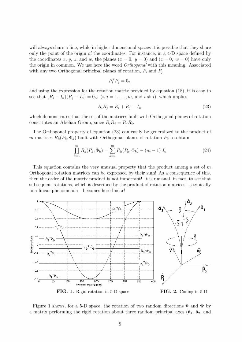
FIG. 1. Rigid rotation in 5-D space FIG. 2. Coning in 5-D

Figure 1 shows, for a 5-D space, the rotation of two random directions v and w bya matrix performing the rigid rotation about three random principal axes (a1, a2, and

9

a3) and by a principal angle varying from 0 to 360◦. This figure shows that the distancevTw, as well as the distances vTak and wTak (k = 1, 2, 3), are all constant during therotation. This means, as stated before, that the directions v and w describe a cone

about the (n − 2)-D subspace defined by A = [a1... a2

... a3] or, equivalently, about the

null space of P = [p1... p2]. The angle between the initial positions, v0 and w0, with the

positions associated with the angle Φ, that is, vΦ = Rv0 and wΦ = Rw0 has a cone-typetypical behavior.

By bending the axes, Figure 2 artistically provides a “way to see” the geometry ofconing about the subspace identified by the three Orthogonal axes a1, a2, and a3.

Orientation Matrices

An orientation matrix C is an n × n proper [det(C)=+1] Orthogonal (CCT = In) ma-trix. The rows of C describe the directions (the axes) of the oriented frame with respectto another frame of reference whose orientation is described by the unity matrix In.In general, an orientation matrix has np complex conjugate eigenvalue pairs λ

(∓)k =

cos Φk ∓ i sin Φk, (k = 1, . . . , np), and na = n− 2np eigenvalues λk = 1, (k = 1, . . . , na).

Associated with the np complex eigenvalues there are np eigenvectors

[√2

2(p

(k)1 ± ip

(k)2 )

]

which identify np proper planes Pk = [p(k)1

... p(k)2 ], while associated with the na real

eigenvalues there are na eigenvectors ak describing na proper axes. Therefore, the eige-nanalysis of an orientation matrix can be expressed as

C

√2

2(p

(k)1 ± ip

(k)2 ) = (cos Φk ± i sin Φk)

√2

2(p

(k)1 ± ip

(k)2 ) (k = 1, . . . , np)

C ak = ak (k = 1, . . . , na)(25)

As it is well known, the orientation can be expressed by a Skew-Symmetric matrix Q,associated to C by the Cayley Transforms‖ (Cayley Conformal Mapping), which consistof the relationships

C =

{= (In −Q)(In + Q)−1

= (In + Q)−1(In −Q)and Q =

{= (In − C)(In + C)−1

= (In + C)−1(In − C)(26)

called forward and inverse transformations, respectively. The matrices C and Q, satis-fying equation (26), have the same eigenvector matrix. In fact, let W be the eigenvectormatrix of C, and ΛC and ΛQ the eigenvalue matrices of C and Q, respectively. SinceC is Orthogonal then W is Orthogonal too, then WW † = In and C = WΛW †. Now,applying the inverse transformation we have

Q = (In − C)(In + C)−1 = (WInW† −WΛCW †)(WInW

† + WΛCW †)−1 == [W (In − ΛC)W †][W (In + ΛC)W †]−1 = W (In − ΛC)(In + ΛC)−1W † = WΛQW †

‖The sign adopted here is such that in 3-D the orientation matrix C coincide with a matrix performingthe rigid rotation about the principal axis by the principal angle, while usually, the coincidence withthe transpose is adopted.

10

which demonstrates that: 1) C and Q have the same eigenvector matrix, and 2) thattheir eigenvalues are related by the bilinear transformation

λ(C) =1− λ(Q)

1 + λ(Q)⇐⇒ λ(Q) =

1− λ(C)

1 + λ(C)

These equations imply the eigenvalue associations

λ(C) = cos Φ± i sin Φ ⇐⇒ λ(Q) = ∓i tan(

Φ

2

)

Actually, Cayley Transforms are nothing else than a bilinear transformation betweenreal matrices.

The eigenanalysis of the Skew-Symmetric orientation matrix Q can, therefore, be writ-ten as

Q

√2

2(p

(k)1 ± ip

(k)2 ) = ∓i tan

(Φk

2

) √2

2(p

(k)1 ± ip

(k)2 ) (k = 1, . . . , np)

Q ak = 0 (k = 1, . . . , na)(27)

The important difference between C and Q consists in the fact that Q may become

singular, which occurs when one (or more) of its eigenvalues λ(Q)k = ∓i tan

(Φk

2

)becomes

infinite.

The eigenanalysis of equations (25) and (27) allows us to provide an expression of Cand Q in terms of their eigenvalues and eigenvectors

C =n∑

k=1

λ(C)k wkw

†k =

na∑

k=1

akaT

k +np∑

k=1

Pk(I2 cos Φk + J2 sin Φk) P T

k

Q =n∑

k=1

λ(Q)k wkw

†k =

np∑

k=1

PkJ2PT

k tan(

Φk

2

)=

np∑

k=1

Ak(Pk) tan(

Φk

2

) (28)

Equation (18) allows us to writenp∑

k=1

Pk(I2 cos Φk + J2 sin Φk) P T

k =np∑

k=1

Rk(Pk, Φk) −

np In +np∑

k=1

PkPT

k and, sincenp∑

k=1

PkPT

k +na∑

k=1

akaT

k = In, we obtain

C =np∑

k=1

Rk(Pk, Φk)− (np − 1) In

Q =np∑

k=1

Sk(Pk, Φk)

(29)

where the matrices

Rk(Pk, Φk) = In + (cos Φk − 1)PkPTk + PkJ2P

Tk sin Φk

Sk(Pk, Φk) = PkJ2PTk tan

(Φk

2

) (30)

11

represents the n × n Skew-Symmetric rotation matrix associated with the Orthogonalrotation matrix Rk(Pk, Φk). Matrices Sk(Pk, Φk) have one pure imaginary eigenvalue pair

λ(Q)k = ∓i tan

(Φk

2

)and a set of (n− 2) eigenvalues λ = 0. Equation (29) demonstrates

that the general rotation, as the planar rotation, depends on the parameters associatedwith its complex eigenvalues/eigenvectors only. Finally, equation (29) allows us to extendthe Euler’s Theorem to any n-D space.

The relationships between Rk(Pk, Φk) and Sk(Pk, Φk) are the classic Cayley Transforms

Rk =

{= (In − Sk)(In + Sk)

−1

= (In + Sk)−1(In − Sk)

Sk =

{= (In −Rk)(In + Rk)

−1

= (In + Rk)−1(In −Rk)

(31)

which remember that C stands to Q (for general rotation) as Rk stands to Sk (for planarrotation), and the exponential relationships

Rk = e[Φk/ tan(Φk/2)] Sk ⇐⇒ Sk =tan(Φk/2)

Φk

ln(Rk) (32)

Extension to the n-D Spaces of the Euler’s Theorem

Equation (29) tells us that the Euler’s Theorem (any orientation can be achieved by onlyone rigid rotation∗∗) is a property that holds in the 2-D and 3-D spaces, only, becausenp = 1. However, this coincidence between geometrical displacement (orientation) andrigid rotation operator (matrix) has also caused the use of orientation and rigid rotationexpressions, without any distinction. These two concepts start differing from one anotherin dimensional spaces greater than three.

Several publications exist which claim to extend the Euler’s Theorem to n-D spaces(see, for instance, [14]), however, most of them actually generalize the dynamics inthe n-D spaces by providing the expression of the angular velocity. Unfortunately, thedynamics problem deal with the orientation of a proper reference frame as a function oftime. On the contrary, Euler’s Theorem is a geometrical property and, therefore, it canbe considered as a static problem. Even in Group Theory, the so called rotation groupactually identify the orientation group of which the set of the rigid rotation matrices isonly a subset. For all these reasons, the confusion between the concepts of orientationand rigid rotation still holds.

As already stated, the n-D rigid rotation is performed about an (n − 2)-D figureidentified by the space spanned by the A matrix. This figure has two perpendicularOrthogonal directions which identify the plane of rotation (matrix P ). Therefore, anydirection belonging to the space spanned by A is not affected by the rotation itself. Thisimplies that only two Orthogonal directions (axes of the reference frame) can be taken

∗∗In Ref. [4], the original latin presentation states that “Quomodocunque sphaera circa centrumsuum conuertatur, semper assignari potest diameter, cuius directio in situ translato conueniat cum situinitiali.”

12

to the final orientation at each subsequent rotation. Therefore, in the most commoncase that there is no axis already at its final position, a number of

⌊n

2

⌋=

{= (n− 1)/2 if n is odd= n/2 if n is even

(33)

rigid rotations are needed in order to reach a given orientation, where the functionbxc rounds x to the nearest integer towards zero. This result can also be derived byanalyzing the eigenvalues of the orientation and the rigid rotation matrices. In fact, inthe n-D space the orientation is identified by a matrix which has, in the most generalcase, n/2 complex conjugate eigenvalue pairs if n is even, or (n−1)/2 complex conjugateeigenvalue pairs and the eigenvalue λ = 1 if n is odd. An n-D rotation matrix has onecomplex conjugate eigenvalue pair (λ(R) = cos Φ ∓ i sin Φ) associated with the planeof rotation (matrix P ), and (n − 2) eigenvalues λ = 1, associated with the principalaxes (matrix A). Now, a multiplication between two n-D rotation matrices (subsequentrotations) outputs a matrix which has, in general, two complex conjugate eigenvaluepairs and (n − 4) eigenvalues λ = 1. This implies that, in order to fill the eigenvaluematrix with complex conjugate eigenvalue pairs, bn/2c subsequent rotations are needed.

Equation (29) and the property given in equation (24) demonstrate that the n × norientation matrix C can be decomposed by a set of np Orthogonal rigid rotation matricesRk(Pk, Φk), whose expression is given in equation (18), that is, by the relationship

C =np∏

k=1

Rk(Pk, Φk) =np∑

k=1

Rk(Pk, Φk)− (np − 1) In (34)

This equation implies that the orientation C can be described by np! different sequencesof Orthogonal rotations, where the Orthogonality is expressed by (i, j = 1, . . . , np, i 6= j)

(Ri − In) (Rj − In) = 0n =⇒ Ri Rj = Ri + Rj − In (35)

The second of equation (29) shows how to decompose the orientation expressed byQ by the sum of a set of np Skew-Symmetric matrices Sk(Pk, Φk). In this case theOrthogonality property is

Si(Pi, Φi) Sj(Pj, Φj) = 0n (36)

Equation (34) is, therefore, nothing else that the mathematical expression of the gener-alized Euler’s Theorem to the n-D spaces. This Theorem can be expressed as follows:

THE GENERALIZED EULER’S THEOREM: Regardless of the way a coordi-nate system is re-oriented from its original orientation, in the n-dimensional space, it isalways possible to find a minimum sequence of np ≤ bn/2c rigid rotations, where np isthe number of complex eigenvalue pairs of the re-orientation matrix, performed on a setof np Orthogonal planes, which ends the initial orientation to the final orientation.

The expression for C given in equation (34) and the expression for Q given in thesecond of equation (29), represent also two new matrix decompositions of the properOrthogonal and of the Skew-Symmetric matrices, respectively. In particular, equation(34) highlights the important fact that subsequent rigid rotations, typically a non linear

13

phenomenon, becomes linear when the rotations matrices constitute an Orthogonal set.In fact, in this case subsequent rigid Orthogonal rotations can be expressed by the suminstead of the product!

For sake of clarity, an example in 4-D space of the decomposition introduced by equa-tion (34), is given in the following.

Numerical Example of Orientation Decomposition

Consider the proper Orthogonal orientation matrix

C =

0.1003 0.2496 −0.8894 −0.36970.9593 −0.0238 −0.0153 0.2810

−0.1172 −0.8638 −0.3828 0.3059−0.2366 0.4370 −0.2495 0.8311

(37)

the eigenanalysis of C yields the eigenvalues (cos Φk ∓ i sin Φk) and the eigenvectors√2

2(p

(k)1 ± ip

(k)2 ) where

{cos Φ1 = −0.7123sin Φ1 = +0.7019

√2

2(p

(1)1 ± ip

(1)2 ) =

0.2923−0.5417−0.2923

0.1888

± i

−0.41680.0499

−0.5629−0.0832

{cos Φ2 = +0.9747sin Φ2 = +0.2235

√2

2(p

(2)1 ± ip

(2)2 ) =

−0.4368−0.4462

0.3036−0.1339

± i

−0.22370.07040.07390.6630

(38)

Associated with the eigenvalues, the principal angles{

Φ1 = ATAN2(sin Φ1, cos Φ1) = 2.3635Φ2 = ATAN2(sin Φ2, cos Φ2) = 0.2254

(39)

are introduced, and associated with the eigenvectors, the principal (rotation) planes

P1 = [p(1)1

... p(1)2 ] and P2 = [p

(2)1

... p(2)2 ], are given

P1 =

0.4134 −0.5894−0.7661 0.0706−0.4134 −0.7961

0.2669 −0.1177

and P2 =

−0.6177 −0.3164−0.6310 0.0995

0.4294 0.1045−0.1893 0.9376

(40)

Now, using equation (18), the rigid rotation matrices

R1(P1, Φ1) =

0.1125 0.3170 −0.9128 −0.23140.9100 −0.0135 0.0024 0.4144

−0.1088 −0.8947 −0.3779 0.2119−0.3840 0.3143 −0.1547 0.8543

(41)

14

and

R2(P2, Φ2) =

0.9878 −0.0674 0.0235 −0.13830.0493 0.9897 −0.0177 −0.1334

−0.0084 0.0309 0.9951 0.09400.1474 0.1226 −0.0948 0.9769

(42)

are obtained. It is easy to see that C = R1R2 = R2R1 = R1 + R2 − I4.

The General Exponential Relationship with Orientation

The Generalized Euler Theorem also allows us to extend the exponential relationship,given in equation (32) and which holds for rigid rotations only, to orientations in n-Dspaces. In fact, equation (32) states that a constant scalar αk, such that Rk = e(αk Sk),exists for rigid rotation, where

αk =Φk

tan(Φk/2)(43)

it is easy to see that it not possible to find a constant scalar α such that C = eα Q.However, the Generalized Euler Theorem provides us a tool to find the closed-formexpression of a general exponential relationship associated with an orientation matrixC. In fact, for general rotation identified by the matrix C, which has eigenvector matrixW , we can write that

C = WΛCW † =np∏

k=1

Rk =np∏

k=1

e(αkSk) = e (∑

kαkSk ) = eWΛEW †

= eE (44)

whereE = WΛEW † (45)

is the Skew-Symmetric exponential matrix which has the same eigenvector matrix of Cand Q, and which has an eigenvalue matrix ΛE with elements ±iΦk. For the sake ofclarity, in the following equation the involved eigenvalues are summarized

ΛC → λ(C)k =

{= cos Φk ± i sin Φk

= 1(np for C, 1 for Rk)(na for C, (n− 2) for Rk)

ΛQ → λQk=

{= ±i tan(Φk/2)= 0

(np for Q, 1 for Sk)(na for Q, (n− 2) for Sk)

ΛE → λEk=

{= ±iΦk

= 0(np for E)(na for E)

(46)

Multiple Rigid Rotations Matrices

The rotation matrix has one complex eigenvalue pair and the remaining (n − 2) areall ones. The product of g ≤ bn/2c Orthogonal rotation matrices output a matrixwhich has, in general, g complex eigenvalue pairs (n ≥ g > 1) while the remaining(n− 2g) eigenvalues are all ones. These matrices perform multiple rigid rotations aboutan (n− 2g)-D subspace.

15

Let us to see an interesting property of these matrices, by analyzing the projection on

the kth plane (Pk) of a rotated point v =

[ g∏

i=1

Ri

]v0, where v0 identifies any position

P T

k v = P T

k

[ g∑

i=1

Ri − (g − 1)In

]v0 = P T

k Rkv0 = (I2 cos Φk + J2 sin Φk)PT

k v0 (47)

which demonstrates that the projected point belong to a circle. Now, varying the anglesΦi, (i = 1, . . . , g), the vertex of the vector v0 describes an g-D surface. The projectionsof this surface on the g Orthogonal planes of rotations are still circles.

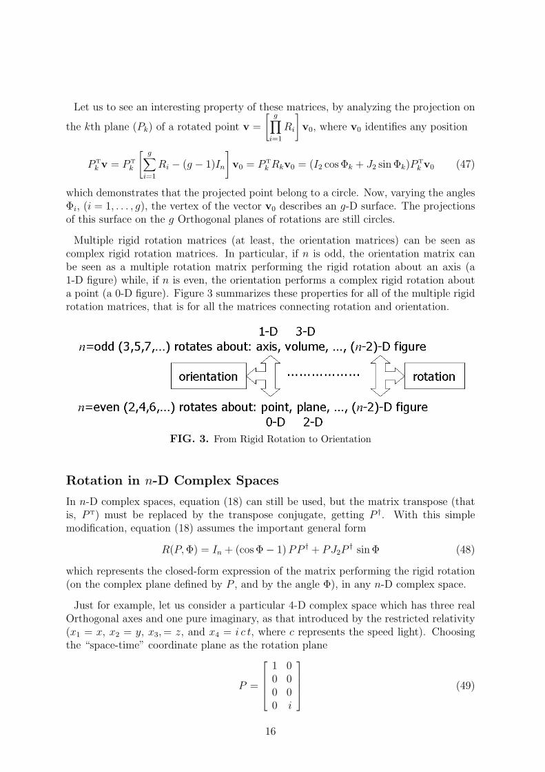
Multiple rigid rotation matrices (at least, the orientation matrices) can be seen ascomplex rigid rotation matrices. In particular, if n is odd, the orientation matrix canbe seen as a multiple rotation matrix performing the rigid rotation about an axis (a1-D figure) while, if n is even, the orientation performs a complex rigid rotation abouta point (a 0-D figure). Figure 3 summarizes these properties for all of the multiple rigidrotation matrices, that is for all the matrices connecting rotation and orientation.

FIG. 3. From Rigid Rotation to Orientation

Rotation in n-D Complex Spaces

In n-D complex spaces, equation (18) can still be used, but the matrix transpose (thatis, P T) must be replaced by the transpose conjugate, getting P †. With this simplemodification, equation (18) assumes the important general form

R(P, Φ) = In + (cos Φ− 1) PP † + PJ2P† sin Φ (48)

which represents the closed-form expression of the matrix performing the rigid rotation(on the complex plane defined by P , and by the angle Φ), in any n-D complex space.

Just for example, let us consider a particular 4-D complex space which has three realOrthogonal axes and one pure imaginary, as that introduced by the restricted relativity(x1 = x, x2 = y, x3, = z, and x4 = i c t, where c represents the speed light). Choosingthe “space-time” coordinate plane as the rotation plane

P =

1 00 00 00 i

(49)

16

then, the rigid rotation matrix can be simply obtained using equation (48)

R =

cos Φ 0 0 −i sin Φ0 1 0 00 0 1 0

−i sin Φ 0 0 cos Φ

(50)

In the complex space, the n× n Skew-Symmetric rotation matrix S(P, Φ), associatedwith the rotation matrix R(P, Φ), becomes Skew-Hermitian

S(P, Φ) = P J2 P † tan(

Φ

2

)(51)

Analogously, the decompositions provided for n-D real spaces, by means of equation (34)for C, and by the second of equation (29) for Q, still hold for n-D complex spaces, butR(P, Φ) and S(P, Φ) must be evaluated by using equations (48) and (51), respectively.

The Ortho-Skew and the Ortho-Skew-Hermitian Matrices

It is known that a proper Orthogonal matrix C has the eigenvalues, λ(∓)k = cos Φk ∓

i sin Φk, which all belong to the unit-radius circle. The eigenvalues of the associatedSkew-Symmetric matrix Q consists of pure imaginary pairs λ

(∓)k = ∓i tan(Φk/2). In

particular, for Symmetricity, when the dimensional space is odd, then C has one eigen-value λ = 1, while the Q matrix has one eigenvalue λ = 0.

FIG. 4. Eigenvalue existence field of the Ortho-Skew-Hermitian matrices

The intersection between the unit-radius circle with the imaginary axis (see Fig. 4)represents, therefore, the field of existence of a set of matrices which are both Orthogonal

17

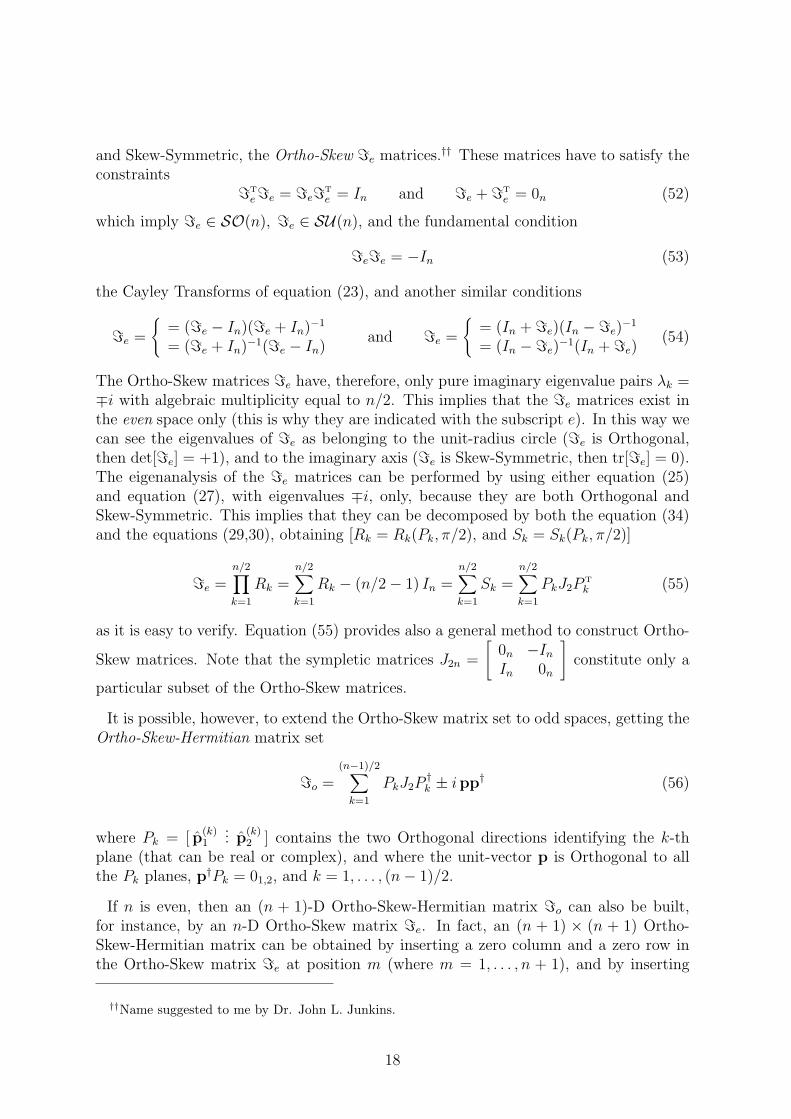
and Skew-Symmetric, the Ortho-Skew =e matrices.†† These matrices have to satisfy theconstraints

=T

e=e = =e=T

e = In and =e + =T

e = 0n (52)

which imply =e ∈ SO(n), =e ∈ SU(n), and the fundamental condition

=e=e = −In (53)

the Cayley Transforms of equation (23), and another similar conditions

=e =

{= (=e − In)(=e + In)−1

= (=e + In)−1(=e − In)and =e =

{= (In + =e)(In −=e)

−1

= (In −=e)−1(In + =e)

(54)

The Ortho-Skew matrices =e have, therefore, only pure imaginary eigenvalue pairs λk =∓i with algebraic multiplicity equal to n/2. This implies that the =e matrices exist inthe even space only (this is why they are indicated with the subscript e). In this way wecan see the eigenvalues of =e as belonging to the unit-radius circle (=e is Orthogonal,then det[=e] = +1), and to the imaginary axis (=e is Skew-Symmetric, then tr[=e] = 0).The eigenanalysis of the =e matrices can be performed by using either equation (25)and equation (27), with eigenvalues ∓i, only, because they are both Orthogonal andSkew-Symmetric. This implies that they can be decomposed by both the equation (34)and the equations (29,30), obtaining [Rk = Rk(Pk, π/2), and Sk = Sk(Pk, π/2)]

=e =n/2∏

k=1

Rk =n/2∑

k=1

Rk − (n/2− 1) In =n/2∑

k=1

Sk =n/2∑

k=1

PkJ2PT

k (55)

as it is easy to verify. Equation (55) provides also a general method to construct Ortho-

Skew matrices. Note that the sympletic matrices J2n =

[0n −In

In 0n

]constitute only a

particular subset of the Ortho-Skew matrices.

It is possible, however, to extend the Ortho-Skew matrix set to odd spaces, getting theOrtho-Skew-Hermitian matrix set

=o =(n−1)/2∑

k=1

PkJ2P†k ± ipp† (56)

where Pk = [ p(k)1

... p(k)2 ] contains the two Orthogonal directions identifying the k-th

plane (that can be real or complex), and where the unit-vector p is Orthogonal to allthe Pk planes, p†Pk = 01,2, and k = 1, . . . , (n− 1)/2.

If n is even, then an (n + 1)-D Ortho-Skew-Hermitian matrix =o can also be built,for instance, by an n-D Ortho-Skew matrix =e. In fact, an (n + 1) × (n + 1) Ortho-Skew-Hermitian matrix can be obtained by inserting a zero column and a zero row inthe Ortho-Skew matrix =e at position m (where m = 1, . . . , n + 1), and by inserting

††Name suggested to me by Dr. John L. Junkins.

18

the imaginary unit ±i in the position =o(m, m). For instance, for m = n, =o can beobtained as

=o =

[=e 0n,1

01,n ± i

](57)

where 0n,1 and 01,n are a column and a row zero vectors with n elements, respectively.Matrix =o is no more either real and Skew-Symmetric, but it is Orthogonal and Skew-Hermitian, since it satisfies the conditions

=†o=o = =o=†o = In and =o + =†o = 0n (58)

and the fundamental condition of (52) still holds as

=o=o = −In (59)

.

Extension of the Imaginary Unit to the Matrix Field

The Ortho-Skew matrices =e are real. This matrix set, together with the Ortho-Skew-Hermitian matrix set =o, can be considered the extension to the matrix field of theimaginary number i =

√−1. In fact, these matrices, since now identified by = (that is,either =e and =o), satisfy most of the known complex identities. They are:

(1) First of all, subsequent powers of i and = follow an identical structure

i k =

+i (for k = 1 + 4m)−1 (for k = 2 + 4m)−i (for k = 3 + 4m)+1 (for k = 4m)

=⇒ = k =

+= (for k = 1 + 4m)−In (for k = 2 + 4m)−= (for k = 3 + 4m)+In (for k = 4m)

(60)

where m can be any integer number.

(2) The = matrices satisfy the Euler’s formula (where eInϑ = Ineϑ)

eϑ+i ϕ = eϑ (cos ϕ + i sin ϕ) =⇒ eInϑ+=ϕ = eInϑ (In cos ϕ + = sin ϕ) (61)

(3) In particular, when ϑ = 0, equation (61) implies a similarity associated with thetrigonometric functions

{2 cos ϕ = ei ϕ + e−i ϕ

2 i sin ϕ = ei ϕ − e−i ϕ =⇒{

2 In cos ϕ = e=ϕ + e−=ϕ

2= sin ϕ = e=ϕ − e−=ϕ (62)

(4) The polar expression of the complex number z = a + i b is

z = ξ (cos ϕ + i sin ϕ) where:

ξ =√

a2 + b2

a = ξ cos ϕb = ξ sin ϕ

(63)

and, analogously, the polar expression of the real matrix Z = In a + = b is

Z = Ξ (In cos ϕ + = sin ϕ) where:

Ξ = In ϑ + =ϕϑ = a cos b + b sin bϕ = −a sin b + b cos b

(64)

19

(5) The similarity for polar expression implies a similarity for the Moivre Formula

zk/j = ξk/j

[cos

(kϕ

j

)+ i sin

(kϕ

j

)](65)

where k and j can be any integer number, to a real matrix form, getting

Zk/j = Ξk/j

[In cos

(kϕ

j

)+ = sin

(kϕ

j

) ](66)

where Z = In a + = b. Note that, for k = 1, and j > k, the Moivre formulacomputes the roots of z while, for j = 1, and k > j, the Moivre formula computesthe powers of z.

Based on the above, it is possible to complete this study by outlining that

i =√−1 is the 1× 1 Ortho-Skew-Hermitian matrix.

Conclusions

This paper presents the general mathematical formulation of the rigid rotation matrix forany n-dimensional real or complex space, and which demonstrates that the rigid rotationis planar in nature. The rigid rotation is shown to depend on an angle (principal angle),which identify the amplitude of the rotation, and on a set of 2 principal axes, identifyingthe plane of rotation, that is, its spatial orientation. This fact suggests us to replace thecommon sentence of rotation about an axis (which holds true in 3-D space only) withthe sentence rotation on a plane, because the plane of rotation is, in fact, an invariantwith respect to the dimensional space. The inverse problem, that is, how to computethese principal rotation parameters from the rotation matrix, is also treated.

Then, Euler’s Theorem is extended to the n-D spaces, by expressing the orientationas a product of a minimum set of rigid rotations. This relationship, which shows thatthe concepts of rigid rotation and orientation become distinct starting from a 4-D space,consists of a new decomposition for proper Orthogonal matrices that can be canonicallyexpressed by either a product or a sum of the same rotation matrix set. A numericalexample of this decomposition for 4-D space is given. Skew-Symmetric matrices, asrepresenting orientation, can also be similarly decomposed by a sum of a set of Skew-Symmetric matrices describing rigid rotations on Orthogonal planes. Then the multiplerigid rotations matrices, which represent the connection path between rigid rotation andorientation, are introduced and the Skew-Symmetric matrix representing the generalexponential relationship with orientation, is also presented.

Finally, the Ortho-Skew real matrices, which are both Orthogonal and Skew-Symmetricand which exist in the even dimensional spaces, and the Ortho-Skew-Hermitian matrices,which are both Orthogonal and Skew-Hermitian and which exist in the odd dimensionalspaces, are introduced. These matrices, which satisfy most of the known complex iden-tities, represent a striking analogy to the imaginary unit for the matrix field.

20

Acknowledgments

This work is dedicated to the memory of Carlo Arduini, deeply missed scientist, teacher,and friend. Carlo, thank you.

The author offers heartfelt thanks to my wife Andreea for her indiscriminate love, tothe poet Silvano Agosti for his freedom of tough, and to John L. Junkins, to whom nothanks can ever be adeguate. I feel indebted also to many important researchers such asF. Landis Markley, Malcolm D. Shuster, and Beny Neta, for many discussions containingdirectly or indirectly contributing to this work.

The author is grateful to the Italian Space Agency for its continued support.

References

[1] RODRIGUEZ, M.O. “Des Lois Geometriques Qui Regissent les Deplacement d’unSysteme Solide dans L’espace, et de la Variation des Coordonnees Provenant de cesDeplacements Consideres Independamment des Causes qui Peuvent les Produire,”Journal de Mathematique Pures et Appliquees (Liouville), 5 (1840), pp. 380-440.

[2] CAYLEY, A. “On the Motion of Rotation of a Solid Body,” Cambridge Mathe-matical Journal, III (1843), pp. 224-232. Also in The Collected Mathematical Pa-pers of Arthur Cayley, I . Cambridge, MA: The Cambridge University Press, 1889.Reprinted by Johnson Reprint Corp., New York, 1963, pp. 28-35.

[3] CAYLEY, A. “On Certain Results Relating to Quaternions,” Cambridge Mathe-matical Journal, III (1843), pp. 131-145. Also in The Collected Mathematical Pa-pers of Arthur Cayley, I . Cambridge, MA: The Cambridge University Press, 1889.Reprinted by Johnson Reprint Corp., New York, 1963, pp. 123-126.

[4] EULER, L. “Formulae Generales pro Trandlatione Quacunque Corporum Rigido-rum,” Novi Acad. Sci. Petrop., 20 (1775), pp. 189-207.

[5] ARCIDIACONO, G. “Relativita e Cosmologia,” Vol. I: Le Teorie Relativistiche diEinstein, Libreria Eredi Virgilio Veschi, Roma, 1979, pp. 24-43, and pp. 54-59.

[6] FANTAPPIE, L. “Su una Nuova Teoria di Relativita Finale,” Rend. Acc. Lincei,ser 8, Vol. 17, fasc. 5 (1954).

[7] CARTAN, E. “Lecons sur la Theorie des Spineurs,” Vol. I, Actualite Scientifiques,n. 643, Paris, Hermann, 1938.

[8] ARCIDIACONO, G. “Relativita e Cosmologia,” Vol. II: Teoria dei Gruppi e Modellidi Universo, Libreria Eredi Virgilio Veschi, Roma, 1979, pp. 11-21.

[9] ABRAHAM, R., MARSDEN, J.E., and RATIU, T. “Manifolds, Tensor Analysis,and Applications,” Springer Verlag, Applied Math Sciences No. 75., 1983, AddisonWesley.

21

[10] LOVELOCK, D., and RUND, H. “Tensors, Differential Forms, and VariationalPrinciples,” Dover Publications, pp. 131-136, 1989.

[11] ARCIDIACONO, G. “Sui Gruppi Ortogonali negli Spazi a Tre, Quattro, CinqueDimensioni,” Portugaliae Mathematica, Vol. 14, fasc. 2, 1955.

[12] ARCIDIACONO, G. “Sulle Trasformazioni Finite dei Gruppi delle Rotazioni,” Coll.Math. XV, 1963, pp. 259-271.

[13] FANTAPPIE, L. “Sulle Funzioni di una Matrice,” Anais da Academia Brasileira deCiencias, n. 1, 26 (1954).

[14] BAR-ITZHACK, I.Y. “Extension of Euler’s Theorem to n-Dimensional Spaces,”IEEE Transactions on Aerospace and Electronic Systems, T-AES/25/6//30692, Vol.25, No. 6, November 1989, pp. 439-517.

[15] SHUSTER, M.D. “A Survey of Attitude Representations,” Journal of the Astro-nautical Sciences, Vol. 41, No. 4, October-December 1993, pp. 439-517.

[16] MORTARI, D. “ESOQ: A Closed-Form Solution to the Wahba Problem,” Journalof the Astronautical Sciences, Vol. 45, No. 2, April-June 1997, pp. 195-204.

[17] MORTARI, D. “n-Dimensional Cross Product and Its Application to Matrix Eige-nanalysis,” Journal of Guidance, Control, and Dynamics, Vol. 20, No. 3, May-June1997, pp. 509-515.

22