On the Representativeness of Norming Samples for … · Therefore, to be useful, the norming sample must be fully representative of the target reference population group on any demographic

4825 Mark Center Drive • Alexandria, Virginia 22311-1850

CAB D0007188.A2/FinalDecember 2003

On the Representativenessof Norming Samples forAptitude Tests

William H. Sims • Catherine M. Hiatt

CNA’s annotated briefings are either condensed presentations of the results of formal CNA studies that have been further documented elsewhere or stand-alone presentations of research reviewed and endorsed by CNA. These briefings repre-sent the best opinion of CNA at the time of issue. They do not necessarily represent the opinion of the Department of the Navy.

Approved for Public Release; Distribution Unlimited. Specific authority: N00014-00-D-0700.For copies of this document call: CNA Document Control and Distribution Section (703) 824-2123.

Copyright 2003 The CNA Corporation

Approved for distribution: December 2003

Henry S. Griffis, DirectorWorkforce, Education and Training TeamResource Analysis Division

1

CNA

On the Representativeness of Norming Samples for Aptitude Tests

31 December 2003

CNA

William H. Sims and Catherine M. Hiatt

This paper discusses the extent to which a sample intended for use in norming aptitude scores must be representative of the underlying population.

This document is part of CNA’s support to the Defense Manpower Data Center (DMDC) on the National Longitudinal Survey of Youth (NLSY97).

2

Summary and conclusions

• A norming sample for the ASVAB (and for similar tests) must be representative of the target reference population with respect to:

• Age, race/ethnicity, and gender• Respondent’s education• Mother’s education

• If the sample is representative with respect to these five variables, it is not necessary that it also be representative with respect to:

• Number of respondents / siblings in household• Degree of urbanization• Census region

Based on the results described in following slides, we conclude that:

• A norming sample for the Armed Services Vocational Aptitude Battery (ASVAB) (and similar tests) must be representative of the targetpopulation with respect to age, race/ethnicity, gender, respondent’s education, and mother’s education.

• It is not necessary that the sample be representative with respect to number of siblings in the household, degree of urbanization, or census region. Although these factors may be correlated to aptitude test scores, if the five other variables are representative, these factors need not be representative.

3

Issue to be addressed

• What demographic variables must be representative of the population in order to have a satisfactory norming sample for aptitude tests?

We address the general question of what variables must be representative of the population in order to have a satisfactory sample of test scores that can be used to norm a test.

Norms for a test describe how a target reference population performs on the test. Therefore, to be useful, the norming sample must be fully representative of the target reference population group on any demographic variable that makes a unique contribution to the variance of test scores.

4

Why are representative test norms important?

• If the norming sample is not representative, then:– Persons selected on the basis of the test

scores may not really have been qualified– Persons denied selection on the basis of

the test scores may really have been qualified

• Defense community plans to use data from NLSY97 to norm ASVAB

Representative test norms are important to any user of test score information. Users might include schools, employers, government, and the military services.

If the norming sample is not representative of the population of interest, persons selected on the basis of test scores may not really have been qualified. Conversely, persons denied selection on the basis of test scores may really have been qualified.

This issue is of particular importance to the defense community given current plans to use aptitude scores collected during the National Survey of Youth (NLSY97) [1] to produce new norms for ASVAB.

5

Approach

• Regression analysis of a nationally representative sample of test scores and demographic information– Determine those demographic

variables that make unique contributions to test score variance

Our approach is to conduct a regression analysis of a nationally representative sample of test scores and demographic information. We will determine those demographic variables that make unique contributions to test score variance.

We stress the phrase “make unique contributions” because it is important to distinguish between the rather large number of variables that are correlated with test scores and that smaller group that uniquely contributes to test score variance. One cannot specify the sample (or develop population weights) on the basis of a very large number of variables because the cell sizes for each combination would be so small that estimates would have large errors.

This work is an extension of our earlier work on the subject [2, 3]. In these earlier reports, we show evidence that age, race, gender, respondent’s education, and mother’s education are important predictors of test scores. However, these reports were very wide ranging and did not focus on the issue ofrepresentativeness of reference or norming populations. In this report, we narrow the focus to the issue of representativeness. We also include additional explanatory variables and develop results for various age and educational subgroups.

6

Data

• We will use PAY80 data– Persons who were part of NLSY79

who tested on ASVAB in 1980 as part of joint DOD/DOL effort

– 11,914 cases– Will focus on AFQT scores as a

measure of general aptitude

We will explore the issue by identifying demographic variables that are correlated with a measure of general aptitude.

We consider the best available sample of nationally representative general aptitude scores to be that collected as part of the Profile of American Youth (PAY) 1980 [4].

The PAY80 sample consists of persons who had participated in the NLSY79 and who agreed to be tested on ASVAB in 1980 as part of a joint effort of the Department of Defense (DOD) and the Department of Labor (DOL). A total of 11,914 persons were tested.

ASVAB contains a measure of general aptitude, known as the Armed Forces Qualification Test (AFQT), along with other tests that measure specific aptitudes.

This analysis will focus on the relationship of AFQT scores to demographic variables. We will assume that variables that correlate with AFQT in 1980 are likely to also correlate in later years.

7

Sample/subsample sizeSize

4,061,0131,2561,27711th grade

3,397,7101,1921,21612th grade

2,169,0726677422-yr college

4,990,2061,4281,5124-yr college

25,585,1727,8019,173Age 18-23

31,452,44410,41911,878PAY80

Case weightedAll variables presentTotal tested1Sample/subsample

1. Excludes 36 cases tested under non-standard conditions.

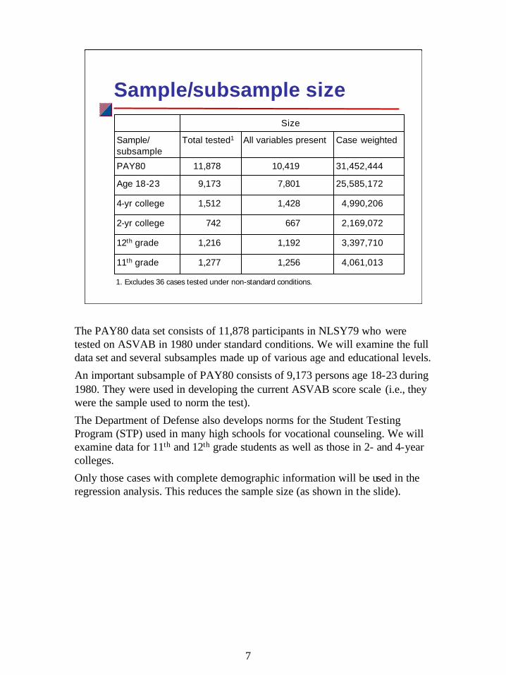
The PAY80 data set consists of 11,878 participants in NLSY79 who were tested on ASVAB in 1980 under standard conditions. We will examine the full data set and several subsamples made up of various age and educational levels.

An important subsample of PAY80 consists of 9,173 persons age 18-23 during 1980. They were used in developing the current ASVAB score scale (i.e., they were the sample used to norm the test).

The Department of Defense also develops norms for the Student Testing Program (STP) used in many high schools for vocational counseling. We will examine data for 11th and 12th grade students as well as those in 2- and 4-year colleges.

Only those cases with complete demographic information will be used in the regression analysis. This reduces the sample size (as shown in the slide).

8

Statistical considerations

• Scale case weights by the design effect to approximate a simple random sample– Allows interpretation of standard regression

statistics

Standard statistical packages produce statistics under the assumption that the data are from a simple random sample (SRS). Neither the 11,914 raw cases or the case weighted sample (approximately 30,000,000) for the PAY80 sample represent the number of cases in an SRS.

Clustering and oversampling both reduce sampling efficiency, but stratification increases sampling efficiency. All three procedures were used in PAY80 and are routinely used in other large sampling efforts.

The design effect is a factor that expresses the inefficiency ofa sample relative to a simple random sample. A sample with a design effect of 1.0 is equivalent to an SRS. A sample with a design effect of 2.0 requires twice as many cases as an SRS to be statistically equivalent to an SRS.

We will scale the sample case weights by the design effect to approximate the size of an equivalent simple random sample. This procedure allows us to interpret the standard regression statistics.

9

Scaling case weights

• Design effect = 1.441+ (.0005056)*(sample size)1

• Effective sample size = sample size/design effect

• Scaled case weight = (case weight/sum of case weights)*

(effective sample size)

1. Relationship developed for the PAY80 data set. See [3].

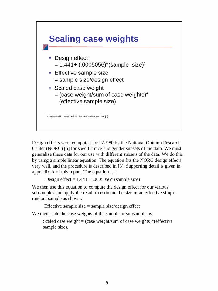
Design effects were computed for PAY80 by the National Opinion Research Center (NORC) [5] for specific race and gender subsets of the data. We must generalize these data for our use with different subsets of the data. We do this by using a simple linear equation. The equation fits the NORC design effects very well, and the procedure is described in [3]. Supporting detail is given in appendix A of this report. The equation is:

Design effect = 1.441 + .0005056* (sample size)

We then use this equation to compute the design effect for our various subsamples and apply the result to estimate the size of an effective simple random sample as shown:

Effective sample size = sample size/design effect

We then scale the case weights of the sample or subsample as:

Scaled case weight = (case weight/sum of case weights)*(effectivesample size).

10

Calculation of SRS sample size

6052.07604,061,0131,25611th grade

5832.04373,397,7101,19212th grade

3751.77822,169,0726672-yr colleges

6602.16304,990,2061,4284-yr colleges

1,4495.385225,585,1727,801Age 18-23

1,5536.708831,452,44410,419PAY80

SRS size3Design effect2

Sum of case weights

Cases1Sample/subsample

1. Cases with complete set of regression variables 2. Design effect = 1.441 + .0005056 (cases) 3. Equivalent simple random sample (SRS) size = cases/design effect

In this slide, we show the calculation of the design effect and equivalent simple random sample size for our sample and various subsamples. We used the equations described on the previous slide.

Note that the design effect ranges from 1.7782 to 6.7088 and that SRS sizes are rather modest in comparison to the raw number of cases. We specifically draw the reader’s attention to the fact that the 10,419 PAY80 cases (with a complete set of regression variables) are statistically equivalent to an SRS of only 1,553 cases.

11

Mean AFQT by age, gender, and race/ethnicity: age 18-23

Age

232221201918

Mea

n A

FQ

T

60

58

56

54

52

50

48

46

44

Gender

Male

Female

Age

232221201918

Mea

n A

FQ

T

70

60

50

40

30

20

Race/ethnicity

White

Hispanic

Black

In the next few slides, we examine mean AFQT by various demographic slices in order to better formulate a regression equation. We focus on the age 18-23 subsample because this is the group of most interest to our sponsor. However, the insights gained will also apply to other subsamples in our study.

The left panel shows mean AFQT by age and by race/ethnicity. The data appear to be linear with age and race/ethnicity.

The right panel shows mean AFQT by age and by gender. There is some indication that the slope of AFQT by age may vary with gender. This result suggests that a cross product of age by gender may be appropriate to include in the regression equation.

12

Mean AFQT by respondent’s education, gender, and race/ethnicity: age 18-23

Respondent's education level

161412111098

Mea

n A

FQ

T

100

80

60

40

20

0

Race/ethnicity

White

Hispanic

Black

Respondent's education level

161412111098

Mea

n A

FQ

T

100

80

60

40

20

0

Gender

Male

Female

The left panel shows mean AFQT by respondent’s education level and race/ethnicity. The data are generally linear with respect to age, respondent’s education, and race/ethnicity. However, there is some indication that the slope of the line may differ for some race/ethnicity groups. This suggests that a race/ethnicity cross product with respondent’s education may be appropriate.

The right panel shows mean AFQT by respondent’s education and gender. The data appear to be linear with respect to respondent’s education and gender.

13

Mean AFQT by mother’s education, gender, and race/ethnicity: age 18-23

Mother's education level

161412111098

Mea

n A

FQ

T

80

70

60

50

40

30

20

Gender

Male

Female

Mother's education level

161412111098

Me

an

AF

QT

80

70

60

50

40

30

20

10

Race/ethnicity

White

Hispanic

Black

The left panel shows mean AFQT by mother’s education level and race/ethnicity. The relationship appears to be generally linear.

The right panel shows mean AFQT by mother’s education and gender. The relationship appears to be generally linear.

14

Regression equation

• AFQT = A + B*(age)+ C*(Black)+ D*(Hispanic)+ E*(male)+ F*(respondent’s edu)+ G*(mother’s edu)+ H*(number of respondent youth in HH)+ I*(urban / rural)+ J*(census region)

NOTE: 1. Several alternative measures were used to capture urban/rural and the number of youth in household (HH).2. Cross terms between race/ethnicity groups, gender, and other variables were also examined in appendix A.

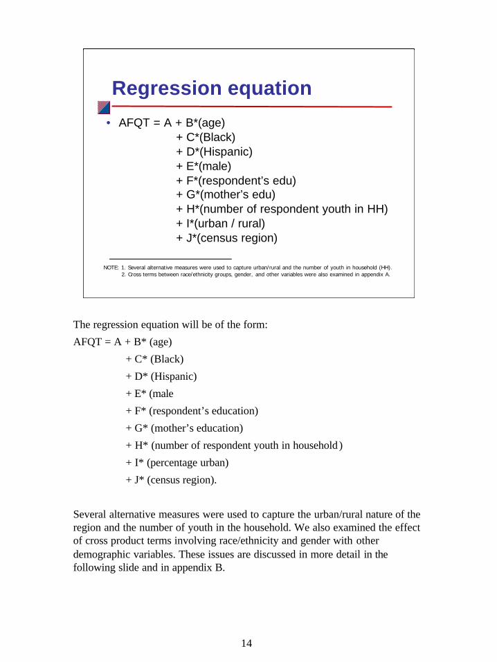
The regression equation will be of the form:

AFQT = A + B* (age)

+ C* (Black)

+ D* (Hispanic)

+ E* (male

+ F* (respondent’s education)

+ G* (mother’s education)

+ H* (number of respondent youth in household )

+ I* (percentage urban)

+ J* (census region).

Several alternative measures were used to capture the urban/rural nature of the region and the number of youth in the household. We also examined the effect of cross product terms involving race/ethnicity and gender with other demographic variables. These issues are discussed in more detail in the following slide and in appendix B.

15

Minor issues

• Alternative definitions:– Urban nature of area

• We used percent urban– Number of respondents / siblings

• We used number of respondents in household

• Census regions• New England region was statistically significant

but of no practical significance

• Race/ethnicity and gender cross products• None were statistically significant

In this slide, we discuss and dismiss a number of minor issues. Appendix B contains details of our findings.

We examined several alternative definitions of the urban nature of the residence and the number of siblings.

We chose to use percent urban rather than SMSA categories because it gave a slightly higher r2 contribution in the regression.

We chose to use number of respondents in the household rather than number of siblings because the r2 contributions were very similar and the number of respondents was much more straightforward to calculate.

We included census region as an explanatory variable in all regressions. Only the New England region showed statistical significance. It was of no practical significance, however, as the contribution to r2 was negligible.

Race/ethnicity cross products with other demographics were also included in the regressions. None were found to be statistically significant.

16

AFQT regression: PAY80 sample

.440

.440

.438

.384

.183

Cum r2

.000

.002

.054

.201

.183

Delta r2

.0931.72.3Urban area

.007-2.7-1.6Youth in household

.00012.03.3Mother’s edu.

.00018.27.9Respondent’s edu.

.0122.52.8Male

.000-4.9-11.7Hispanic

.000-15.1-25.0Black

.000-7.7-2.6Age

.000-4.6-26.0Constant

Signif.T-stat.CoefficientVariable

NOTE: All r2 are adjusted r2 and variables statistically significant at the .05 level are in bold type

This slide summarizes the regression results for the full PAY80 sample. The sample includes persons age 16 to 23 in 1980. These persons were age 15 to 22 in 1979 when the original NLSY79 survey data were collected.

The slide shows the regression coefficients, T-statistics, significance, cumulative adjusted r2, and incremental change in adjusted r2 as the variable, or groups of variables, were entered into the regression.

Age, race/ethnicity, and gender were entered as a group. They are all statistically significant and contribute 0.183 to the r2. Respondent’s education is statistically significant and adds 0.201 to the r2, increasing it to 0.384. Mother’s education is statistically significant and adds anothe r 0.054 to the r2, increasing it to 0.438. The number of youth in the household is also statistically significant but only adds a negligible 0.002 to the r2. Percentage urban is not statistically significant.

The slide does not include any discussion of census regions or race/ethnicity cross products because they are either not statistically significant or they have a negligible effect on r2. See appendix B for more detail on these issues.

17

AFQT regression: Age 18-23 subsample

.464

.464

.461

.442

.174

Cum r2

.000

.003

.039

.248

.174

Delta r2




.00020.08.3Respondent’s edu.

.0003.53.9Male

.000-5.0-12.4Hispanic

.000-14.9-25.4Black

.000-5.2-1.9Age

.000-5.5-40.3Constant


This slide summarizes the regression results for the age 18-23 subsample. These individuals were age 18-23 when they were tested on ASVAB in 1980.

We see that age, race/ethnicity, gender, respondent’s education, and mother’s education are all statistically significant and make meaningful incremental contributions to r2. The number of youth in the household is statistically significant but does not make a meaningful contribution to r2.

18

AFQT regression: 4-year college subsample

.294

.295

.297

NA

.252

Cum r2

-.001

-.002

.045

NA

.252

Delta r2

.815-0.2-0.4Urban area



NANANARespondent’s edu.

.0004.05.6Male

.001-3.3-12.9Hispanic

.000-12.8-29.4Black

.3950.90.4Age

.0003.640.4Constant


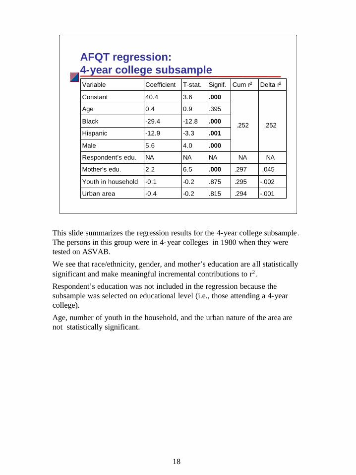
This slide summarizes the regression results for the 4-year college subsample. The persons in this group were in 4-year colleges in 1980 when they were tested on ASVAB.

We see that race/ethnicity, gender, and mother’s education are all statistically significant and make meaningful incremental contributions to r2.

Respondent’s education was not included in the regression because the subsample was selected on educational level (i.e., those attending a 4-year college).

Age, number of youth in the household, and the urban nature of the area are not statistically significant.

19

AFQT regression: 2-year college subsample

.286

.270

.271

NA

.248

Cum r2

.015

-.001

.023

NA

.248

Delta r2


.8490.20.2Youth in household



.0023.16.9Male

.000-4.2-19.0Hispanic

.000-9.2-32.4Black

.0182.41.9Age

.682-0.4-7.5Constant


This slide summarizes the regression results for the 2-year college subsample. The persons in this group were in 2-year colleges in 1980 when they were tested on ASVAB or had been in 2-year colleges the previous year.

We see that age, race/ethnicity, gender, and mother’s education are all statistically significant and make meaningful incremental contributions to r2.

Respondent’s education was not included in the regression because the subsample was selected on educational level (i.e., those attending a 2-year college).

The number of youth in the household is not statistically significant. Urban area is statistically significant. It contributes 0.015 to r2.

20

AFQT regression: 12th grade subsample

.304

.304

.305

NA

.245

Cum r2

.000

.001

.060

NA

.245

Delta r2





.0442.03.8Male

.016-2.4-9.7Hispanic

.000-9.4-25.9Black

.000-6.2-7.1Age

.0006.5128.9Constant


This slide summarizes the regression results for the 12th grade subsample. The persons in this group were expected to enter the 12th grade in the fall of 1980, having been tested on ASVAB during the summer of 1980.

We see that age, race/ethnicity, gender, and mother’s education are all statistically significant and make meaningful incremental contributions to r2.

Respondent’s education was not included in the regression because the subsample was selected on a specific educational level (i.e., those expected to be in the 12th grade in the fall of 1980).

Number of youth in the household and the urban nature of the area are not statistically significant.

21

AFQT regression: 11th grade subsample

.313

.309

.307

NA

.183

Cum r2

.004

.002

.124

NA

.183

Delta r2





.409-0.8-1.5Male

.005-2.8-11.2Hispanic

.000-9.8-26.3Black

.020-2.3-6.6Age

.0352.197.9Constant


This slide summarizes the regression results for the 11th grade subsample. The persons in this group were expected to enter the 11th grade in the fall of 1980, having been tested on ASVAB during the summer of 1980.

We see that age, race/ethnicity, and mother’s education are all statistically significant and make meaningful incremental contributions to r2.

Respondent’s education was not included in the regression because the subsample was selected on a specific educational level (i.e., those expected to be in the 12th grade in the fall of 1980).

Number of youth in the household is not statistically significant. Urban area is statistically significant but contributes a negligible amount to r2.

Interestingly, gender is not statistically significant for 11th grade, although it was for 12th grade. This result suggests that strong gender effects begin toemerge late in high school.

22

Summary of regression coefficients

4.5NS4.7NANS-11.2-26.3-6.611th grade

NSNS3.1NA3.8-9.7-25.9-7.112th grade

10.1NS1.7NA6.9-19.0-32.41.92-yr col

NSNS2.2NA5.6-12.9-29.4NS4-yr col

NS-1.62.98.33.9-12.4-25.4-1.9Age 18-23

NS-1.63.37.92.8-11.7-25.0-2.6PAY80

UrbanYouth/HH

Mom’s edu

Resp.edu

MaleHispBlackAgeSample/ subsample

NOTE: NS = not statistically significant at the .05 level, NA = not applicable

Here, we draw together the coefficients from regressions on all samples. For example, one additional year of mother’s education is associated with an increase in AFQT of 4.7 percentile points for 11th grade youth. The results are generally consistent, and the trends that emerge appear reasonable.

The coefficient on age is generally negative. This finding is reasonable to expect when respondent’s educational level is held constant either by regression (as in the PAY80 sample and age 18-23 subsample) or by selection (as in the other subsamples). Presumably, the older persons in a particular educational group are more likely to have been held back for lack of performance and, hence, would be expected to have lower AFQT scores. The reason for the positive age coefficient for the 2-year college sample is unclear but it does represent persons in the first and second year of college.

Coefficients for race and ethnicity are generally constant over all samples. Males do better than females except for the 11th grade subsample. This finding is consistent with an onset of strong gender differences late in the high school.

Respondent’s education is consistently important where applicable. Mother’s education is always a factor but seems to be most important in the high school subsamples, particularly in the 11th grade.

The number of youth respondents in the household is statistically significant only for the entire PAY80 sample and for the age 18-23 subsample.

Urban area is statistically significant for 2-year colleges and 11th grade. The lack of consistency over subsamples makes this result somewhat suspect.

23

Summary of explained variance (r2)

.313.004.002.124NA.18311th grade

.304.000.001.060NA.24512th grade

.286.015-.001.023NA.2482-yr col

.294-.001-.002.045NA.2524-yr col

.464.000.003.039.248.174Age 18-23

.440.000.002.054.201.183PAY80

TotalUrbanYouth/HH

Mom’s edu

Resp. edu

Age, gender and race/ethnicity

Sample/subsample

Increment to r2 by indicated variable

On this slide, we draw together the contribution to explained variance for the sample and subsamples. Again, the results are generally consistent across groups:

1. The combination of age, gender, and race/ethnicity consistently contributes about 0.2 to the r2.

2. Respondent’s education contributes another 0.2 to r2.

3. Mother’s education contribution to r2 ranges from a low of 0.023 for 2-year college students to 0.124 for 11th grade students. This variable appears to be more important for high school students than for others.

4. The contribution to r2 by number of respondents per household is consistently negligible.

5. The urban nature of the area makes a negligible contribution to r2 except for 2-year college students. The lack of consistency in this result suggests that it should be viewed with some skepticism.

24

Conclusion

• An AFQT norming sample must be representative of the population with respect to:

• Age, race/ethnicity, and gender• Respondent’s education• Mother’s education

• If that is true, it is not necessary that it also be representative by:

• Number of respondents / siblings in household• Degree of urbanization• Census region

Based on the results described above, we conclude the following.

An AFQT norming sample must be representative of the target population with respect to age, race, gender, respondent’s education, and mother’s education. Mother’s education is particularly important for high school norms.

If the sample is representative on the five variables noted above, it is not necessary that it also be representative by number of respondents, degree of urbanization, or census region.

25

Appendix A: Design effect

In this appendix, we include details on the estimation of design effects for the various subsamples. NORC computed the design effect for the PAY80 sample and for several race and gender subsamples. However, for our analysis, we needed to generalize the design effect to other subsamples.

26

What is the design effect?

• It is a factor that expresses the inefficiency of a sample relative to a simple random sample:– Clustering reduces sampling efficiency– Oversampling reduces sampling efficiency– Stratification increases sampling efficiency

• Effective sample size is estimated as:– Actual sample size /design effect

• Why do we need to know it?– We need it to estimate statistical errors in PAY80

The design effect is a factor that expresses the inefficiency ofa sample relative to a simple random sample (SRS). A sample with a design effect of 1.0 is equivalent to an SRS. A sample with a design effect of 2.0 requires twice as many cases as an SRS to be statistically equivalent to an SRS.

Both clustering and oversampling reduce sampling efficiency, butstratification increases sampling efficiency. All three procedures were used in PAY80 and are routinely used in other large sampling efforts.

Effective sample size (i.e., size of an equivalent simple random sample) is the actual sample size divided by the design effect.

The PAY80 data set is based on about 12,000 cases and weighted by case weights to approximate the total youth population of about 30,000,000. Neither the raw number of cases nor the weighted number of cases is appropriate for use in statistical tests because neither represents an SRS (which is assumed by most common statistical packages). For this reason, we must use the design effect to estimate new scaled case weights that will approximate an SRS.

27

Design effect for mean AFQT in PAY80a

7.4373

4.5057

2.2091

2.1147

2.9946

4.6307

2.1018

1.8253

3.2164

Design effect

11,914

5,945

935

1,511

3,499

5,969

908

1,517

3,544

Number of cases

Total

Subtotal

Hispanic

Black

WhiteFemale

Subtotal

Hispanic

Black

WhiteMale

Race/ethnicityGender

a. NORC, Profile of American Youth, User’s Guide and Codebook , March 1982

This slide shows the design effects calculated by NORC [5] for major race and gender subsamples within the PAY80 sample.

28

Design effect and sample size: PAY80

Number of cases

14000120001000080006000400020000

Des

ign

effe

ct

8

7

6

5

4

3

2

1

0

BMBF

HMHF

WMWF

MF

Total

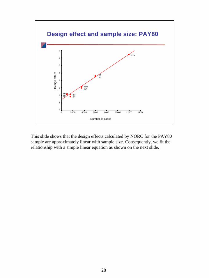
This slide shows that the design effects calculated by NORC for the PAY80 sample are approximately linear with sample size. Consequently, we fit the relationship with a simple linear equation as shown on the next slide.

29

Regression on PAY80 design effect

.00022.430.000.0005056Number of cases

.00012.275.1171.441Constant

SignificanceT-statisticStandard error

CoefficientVariable

NOTE: The r2 for the fit was .99 and the standard error of estimate was 0.23

This slide shows the details of the regression on design effect in PAY80. Based on these results, we will use the following equation to estimate design effects for the various subsamples in our analysis:

Design effect = 1.441 + 0.0005056 (number of cases) .

30

31

Appendix B: Statistical detail

This appendix contains backup slides with additional statistical detail.

32

Means for main variables: PAY80 sample and subsamples

.75.77.88.84.79.78Urban

1.891.931.901.931.891.89Youth/hh

11.8312.0012.4313.0711.8011.79Mom’s edu

NANANANA11.9711.28Resp. edu.

.51.51.43.51.49.50Male

.06.06.07.03.06.06Hisp.

.14.14.11.10.13.13Black

16.0616.4720.5220.7920.2319.17Age

42.7347.1260.5176.6951.0848.83AFQT

11th grade12th grade2-yr. col.4-yr. col.Age 18-23PAY80Variables

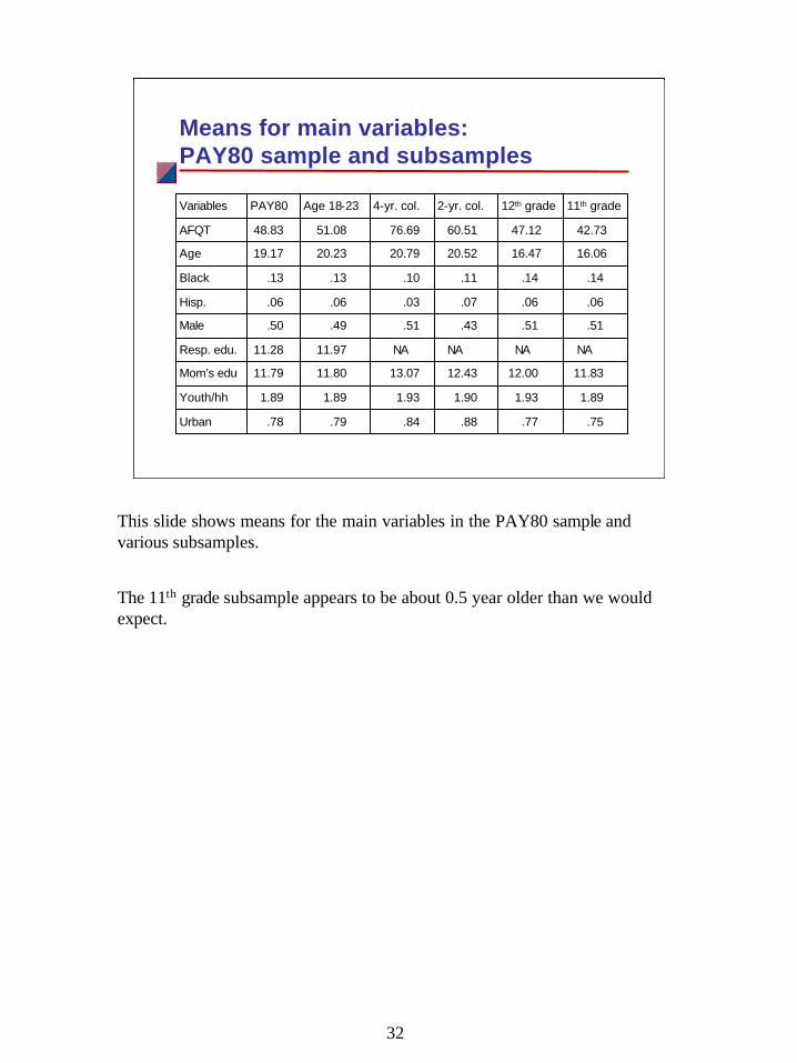
This slide shows means for the main variables in the PAY80 sample and various subsamples.

The 11th grade subsample appears to be about 0.5 year older than we would expect.

33

Standard deviations for main variables: PAY80 sample and subsamples

.43.42.33.37.41.41Urban

.92.94.91.92.94.94Youth/hh

2.092.202.092.112.192.19Mom’s edu

NANANANA1.661.91Resp. edu.

.50.50.50.50.50.50Male

.24.25.25.18.24.24Hisp.

.35.35.31.31.34.34Black

0.330.841.371.401.772.39Age

27.1226.8224.5821.0628.9528.87AFQT

11th grade12th grade2-yr. col.4-yr. col.Age 18-23PAY80Variables

This slide shows the standard deviations of the main variables in the PAY80 sample and subsamples.

Note that the standard deviation for the 11th grade sample is 0.3. This small standard deviation, coupled with the higher than expected mean age shown on the previous slide, suggests that the youngest of the 11th grade youth may be missing.

34

Correlation matrix for main variables: age 18-23 subsample

1.00.05.00.02.04.02.08-.11-.06Youth/hh

.051.00.09.11-.00.09.06.03.06Urban

.00.091.00.35-.05-.10-.08.46.53Resp. edu.

.02.11.351.00.03-.23-.12.00.45Mom’s edu.

.04-.00-.05.031.00.00-.01-.02.05Male

.02.09-.10-.23.001.00-.10-.01-.17Hisp.

.08.06-.08-.12-.01-.101.00-.03-.35Black

-.11.03.46.00-.02-.01-.031.00.12Age

-.06.06.53.45.05-.17-.35.121.00AFQT

Youth/ hh

UrbanResp. edu.

Mom’s edu.

MaleHisp.BlackAgeAFQT

NOTE: correlations significant at the .05 level are shown in bold type.

This slide shows the correlation matrix for the main variables in the age 18-23 subsample. We focus on the age 18-23 group in this and the following slides because it is of most interest to our sponsor. The data for other subsamples are similar.

Those correlations that are significant at the .05 level are shown in bold type.

Mother’s education and respondent’s education are both strongly correlated with AFQT. Respondent’s education is strongly correlated with respondent’s age and mother’s education. Mother’s education is strongly correlated with respondent’s education but not with respondent’s age. Race/ethnicity also correlates strongly with AFQT.

35

r2 by various definitions of urban and siblings:age 18-23 subsample

.477 (NS)

.476 (NS)

.477 (NS)

.479 (NS)

.478(NS)

.479 (NS)

Above + urban

.475.475.475.478.477.478Above + # youth/hh

.472.472.472.474.474.474Above + mom’s edu

.432.432.432.435.435.435Above + resp. edu

.188.188.188.189.189.189Gender, race, age

Youth = # resp. 18-23

Youth = # resp.

Youth = # sibs

Youth = # resp.18-23

Youth = # resp.

Youth = # sibs

Variables

Urban = SMSA groupsUrban = % urban

Denotes results for variable definitions used in this analysis. Sample sizes are slightly different from those in the main analy sis.

We estimated the regression equation:

AFQT = A + Σi (Bi Xi) ,where A and Bi are constants and Xi are independent variables.

Regression results are shown for six combinations of measures of numbers of respondent youth and urban nature of the region. For number of youth, we use the total number of siblings of all ages, the total number of respondent youth in the survey, and the total number of respondent youth age 18-23. For urban nature, we use the urban / rural designation as well as the four SMSA groups. The four SMSA groups are as follows: not SMSA, SMSA not center city, SMSA center city, and SMSA unknown center city. All combinations gave essentially the same results.

The slide shows cumulative percentage of variance explained (r2) as different variables are added to the regression. At the first stage we include the basic variables of gender, race, and age. We then add respondent’s education, then mother’s education, then a measure of the number of youth in the household, and finally a measure of the urban nature of the region. All variables were statistically significant at the .05 level except for measures of the urban nature of the region.

We decided to use percentage urban as the measure of urbanization because it is simple to use and gave a slightly larger r2. We decided to use the number of respondent youth in the household as a measure of siblings because it is easiest to calculate.

36

Regression results for census regions:age 18-23 subsample

.084-1.7-3.8CR Pacific

.507-0.7-1.9CR Mountain

.828-0.2-0.5CR West South Central

.162-1.4-3.9CR East South Central

.150-1.4-2.8CR South Atlantic

.4560.71.9CR West North Central

.699-0.4-0.7CR East North Central

.0282.26.2CR New England

.003.467

.5630.69.9CR Other

.464.464NANANAOthers1

Delta r2Cum r2Signif.T-Stat.CoefficientVariable

1. Age, race/ethnicity, gender, respondent’s edu, mom’s edu, youth/HH, urban

This slide summarizes the effect of adding dummy variables to represent census regions. Census region Mid Atlantic is subsumed in the constant.

The first row shows the cumulative r2 for the main variables of age, race/ethnicity, gender, respondent’s education, mother’s education, number of respondent youth per household, and percent urban. Other rows show the effect of adding the census region dummy variables.

Only the variable for census region New England was statistically significant. However, all of the census region variables together added only 0.003 to the r2. We consider that effect to be negligible. Census region variable s were not included in the final regressions shown in the main text.

37

Race/ethnicity and gender cross terms:age 18-23 subsample

.7680.30.2Male x age

.6890.40.9Hisp x youth/HH

.727-0.3-3.4Hisp x urban

.9090.10.1Hisp x mom’s education

.354-0.9-1.4Hisp x respondent’s education

.8450.20.9Hisp x male

.6570.40.7Hisp x age

.489-0.7-1.1Black x youth/HH

.548-0.6-2.8Black x urban

.179-1.3-1.2Black x mom’s education

.051-2.0-2.3Black x respondent’s. education

.636-0.5-1.6Black x male

.000.467

.7110.40.4Black x age

.467.467NANANAAll other variables

Delta r2Cum. r2Signif.T-Stat.Coeff.Variables

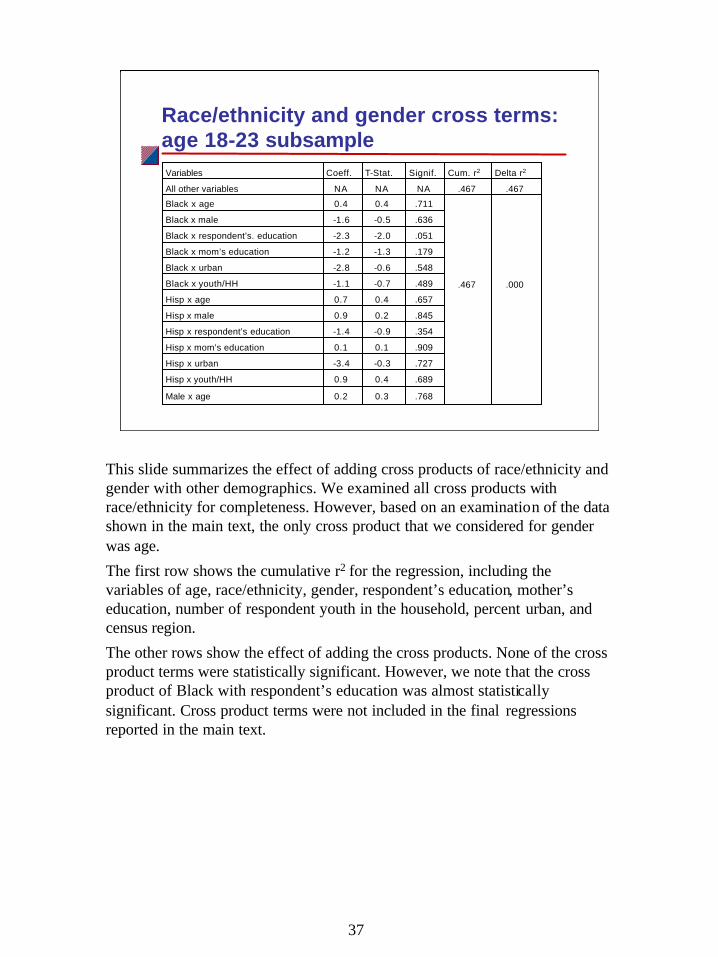
This slide summarizes the effect of adding cross products of race/ethnicity and gender with other demographics. We examined all cross products with race/ethnicity for completeness. However, based on an examination of the data shown in the main text, the only cross product that we considered for gender was age.

The first row shows the cumulative r2 for the regression, including the variables of age, race/ethnicity, gender, respondent’s education, mother’s education, number of respondent youth in the household, percent urban, and census region.

The other rows show the effect of adding the cross products. None of the cross product terms were statistically significant. However, we note that the cross product of Black with respondent’s education was almost statistically significant. Cross product terms were not included in the final regressions reported in the main text.

38

39

References

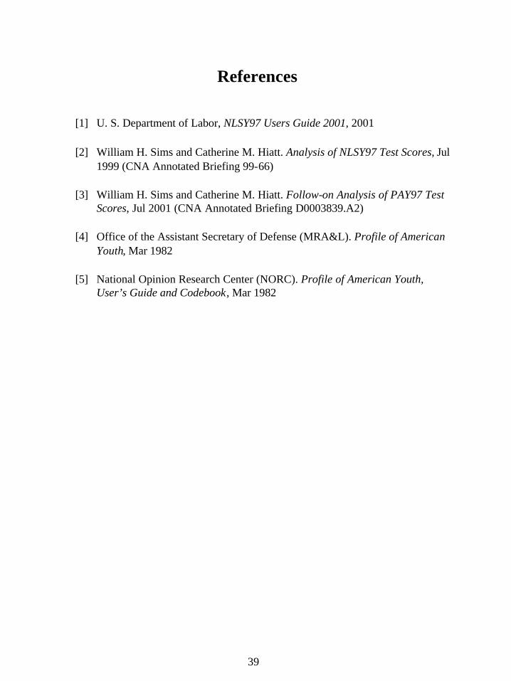
[1] U. S. Department of Labor, NLSY97 Users Guide 2001, 2001

[2] William H. Sims and Catherine M. Hiatt. Analysis of NLSY97 Test Scores, Jul 1999 (CNA Annotated Briefing 99-66)

[3] William H. Sims and Catherine M. Hiatt. Follow-on Analysis of PAY97 Test Scores, Jul 2001 (CNA Annotated Briefing D0003839.A2)

[4] Office of the Assistant Secretary of Defense (MRA&L). Profile of American Youth, Mar 1982

[5] National Opinion Research Center (NORC). Profile of American Youth, User’s Guide and Codebook, Mar 1982

40

CA

B D

0007

188

.A2

/Fin

al

Documents

On the Representativeness of Norming Samples for … · Therefore, to be useful, the norming sample must be fully representative of the target reference population group on any demographic