On the Power of Randomization in Big Data Analytics including nearest neighbor search, outlier detection and classifica-tion. Theseconceptsarealsobasicdataanalysisproblemsthatthethesisaims

On the Power of Randomization

in Big Data Analytics

Phạm Đăng Ninh

Theoretical Computer Science Section

IT University of Copenhagen, Denmark

A thesis submitted for the degree of

Doctor of Philosophy

31/08/2014

ii

Acknowledgements

No guide, no realization.

First of all I am deeply grateful to Rasmus Pagh, a very conscientiousadvisor that I could ever ask or even hope for. He is patient enough totake the time to listen to my ideas, good as well as bad, and to sharehis thoughts, basic as well as advanced. He is open-minded enoughto guide me to find such a good balance between computational al-gorithms and data analysis, which inspired the principle of the thesiscontribution. Rasmus is not only a superb teacher but also a greatcolleague.

A special thank you goes to Hoàng Thanh Lâm, a very enthusiasticfriend, who provided me constant support and encouragement, fromcomments on finding the PhD scholarship and preparing specific re-search background - to discussions about data mining challenges andadvices on how to grow scientific research network. Without his helpmy PhD would have remained incomplete.

I also thank to my colleagues, Thore Husfeldt, Jesper Larsson, Kon-stantin Kutzkov, Nina Sofia Taslaman, Andrea Campagna, MortenStockel, Troels Bjerre Sørensen, Francesco Silvestri, Tobias LybeckerChristiani. It is my pleasure to discuss with you about both researchtopics and life experience.

A big thank you goes to my co-author Michael Mitzenmacher forletting me work with him and learn from him.

I gratefully acknowledge IT University of Copenhagen, which pro-vided me a very nice working environment and the Danish NationalResearch Foundation, which gave me the financial support.

I am also grateful to John Langford for his hospitality during myvisit at NYC Microsoft research. I also thank the Center for UrbanScience and Progress (CUSP) for being my host at New York Cityand receiving me so well.

I would like to express my gratitude to my close friends, Lê QuangLộc, Nguyễn Quốc Việt Hùng, Mai Thái Sơn for sharing their PhD

experience, and my Vietnamese friends from Technical University ofDenmark, University of Copenhagen, and Liễu Quán temple, whomade my PhD journey pleasant and memorable.

I would like to thank Aristides Gionis and Ira Assent for acceptingto be the external members of my assessment committee and DanWitzner Hansen for chairing the committee.

Last, but not least, I would like to thank my parents, Phạm Sỹ Hỷ andLê Thị Thanh Hà, with their great upbringing and support throughoutmy life.

Ninh Pham,Copenhagen, July 3, 2014

Abstract

We are experiencing a big data deluge, a result of not only the in-ternetization and computerization of our society, but also the fastdevelopment of affordable and powerful data collection and storagedevices. The explosively growing data, in both size and form, hasposed a fundamental challenge for big data analytics. That is howto efficiently handle and analyze such big data in order to bridge thegap between data and information.

In a wide range of application domains, data are represented as high-dimensional vectors in the Euclidean space in order to benefit fromcomputationally advanced techniques from numerical linear algebra.The computational efficiency and scalability of such techniques havebeen growing demands for not only novel platform system architec-tures, but also efficient and effective algorithms to address the fast-paced big data needs.

In the thesis we will tackle the challenges of big data analytics inthe algorithmic aspects. Our solutions have leveraged simple but fastrandomized numerical linear algebra techniques to approximate fun-damental data relationships, such as data norm, pairwise Euclideandistances and dot products, etc. Such relevant and useful approxima-tion properties will be used to solve fundamental data analysis tasks,including outlier detection, classification and similarity search.

The main contribution of the PhD dissertation is the demonstrationof the power of randomization in big data analytics. We illustrate ahappy marriage between randomized algorithms and large-scale dataanalysis in data mining, machine learning and information retrieval.In particular,

• We introduced FastVOA, a near-linear time algorithm to ap-proximate the variance of angles between pairs of data points, arobust outlier score to detect high-dimensional outlier patterns.

• We proposed Tensor Sketching, a fast random feature mappingfor approximating non-linear kernels and accelerating the train-ing kernel machines for large-scale classification problems.

• We presented Odd Sketch, a space-efficient probabilistic datastructure for estimating high Jaccard similarities between sets, acentral problem in information retrieval applications.

The proposed randomized algorithms are not only simple and easy toprogram, but also well suited to massively parallel computing envi-ronments so that we can exploit distributed parallel architectures forbig data. In future we hope to exploit the power of randomizationnot only on the algorithmic aspects but also on the platform systemarchitectures for big data analytics.

Contents

1 Introduction 1

2 Background 5

2.1 High-dimensional Vectors in the Euclidean Space . . . . . . . . . 6

2.2 Fundamental Concepts in Data Analysis . . . . . . . . . . . . . . 6

2.2.1 Nearest Neighbor Search . . . . . . . . . . . . . . . . . . . 7

2.2.2 Outlier Detection . . . . . . . . . . . . . . . . . . . . . . . 8

2.2.3 Classification . . . . . . . . . . . . . . . . . . . . . . . . . 9

2.3 Core Randomized Techniques . . . . . . . . . . . . . . . . . . . . 11

2.3.1 Tools from Probability Theory . . . . . . . . . . . . . . . . 11

2.3.2 Random Projection . . . . . . . . . . . . . . . . . . . . . . 11

2.3.3 Hashing . . . . . . . . . . . . . . . . . . . . . . . . . . . . 13

3 Angle-based Outlier Detection 19

3.1 Introduction . . . . . . . . . . . . . . . . . . . . . . . . . . . . . . 20

3.2 Related Work . . . . . . . . . . . . . . . . . . . . . . . . . . . . . 21

3.3 Angle-based Outlier Detection (ABOD) . . . . . . . . . . . . . . . 23

3.4 Algorithm Overview and Preliminaries . . . . . . . . . . . . . . . 25

3.4.1 Algorithm Overview . . . . . . . . . . . . . . . . . . . . . 25

3.4.2 Preliminaries . . . . . . . . . . . . . . . . . . . . . . . . . 26

3.5 Algorithm Description . . . . . . . . . . . . . . . . . . . . . . . . 28

3.5.1 First Moment Estimator . . . . . . . . . . . . . . . . . . . 28

3.5.2 Second Moment Estimator . . . . . . . . . . . . . . . . . . 29

3.5.3 FastVOA - A Near-linear Time Algorithm for ABOD . . . 31

v

CONTENTS

3.5.4 Computational Complexity and Parallelization . . . . . . . 32

3.6 Error Analysis . . . . . . . . . . . . . . . . . . . . . . . . . . . . . 33

3.6.1 First Moment Estimator . . . . . . . . . . . . . . . . . . . 34

3.6.2 Second Moment Estimator . . . . . . . . . . . . . . . . . . 35

3.6.3 Variance Estimator . . . . . . . . . . . . . . . . . . . . . . 36

3.7 Experiments . . . . . . . . . . . . . . . . . . . . . . . . . . . . . . 37

3.7.1 Data Sets . . . . . . . . . . . . . . . . . . . . . . . . . . . 37

3.7.2 Accuracy of Estimation . . . . . . . . . . . . . . . . . . . . 38

3.7.3 Effectiveness . . . . . . . . . . . . . . . . . . . . . . . . . . 40

3.7.4 Efficiency . . . . . . . . . . . . . . . . . . . . . . . . . . . 42

3.8 Conclusion . . . . . . . . . . . . . . . . . . . . . . . . . . . . . . . 44

4 Large-scale SVM Classification 45

4.1 Introduction . . . . . . . . . . . . . . . . . . . . . . . . . . . . . . 46

4.2 Related Work . . . . . . . . . . . . . . . . . . . . . . . . . . . . . 48

4.3 Background and Preliminaries . . . . . . . . . . . . . . . . . . . . 49

4.3.1 Count Sketch . . . . . . . . . . . . . . . . . . . . . . . . . 49

4.3.2 Tensor Product . . . . . . . . . . . . . . . . . . . . . . . . 51

4.4 Tensor Sketching Approach . . . . . . . . . . . . . . . . . . . . . 52

4.4.1 The Convolution of Count Sketches . . . . . . . . . . . . . 52

4.4.2 Tensor Sketching Approach . . . . . . . . . . . . . . . . . 54

4.5 Error Analysis . . . . . . . . . . . . . . . . . . . . . . . . . . . . . 55

4.5.1 Relative Error Bound . . . . . . . . . . . . . . . . . . . . . 55

4.5.2 Absolute Error Bound . . . . . . . . . . . . . . . . . . . . 57

4.5.3 Normalization . . . . . . . . . . . . . . . . . . . . . . . . . 57

4.6 Experimental Results . . . . . . . . . . . . . . . . . . . . . . . . . 58


4.6.2 Efficiency . . . . . . . . . . . . . . . . . . . . . . . . . . . 59

4.6.3 Scalability . . . . . . . . . . . . . . . . . . . . . . . . . . . 61

4.6.4 Comparison with Heuristic H0/1 . . . . . . . . . . . . . . 67

4.7 Conclusion . . . . . . . . . . . . . . . . . . . . . . . . . . . . . . . 68

vi

CONTENTS

5 High Similarity Estimation 69

5.1 Introduction . . . . . . . . . . . . . . . . . . . . . . . . . . . . . . 70

5.1.1 Minwise Hashing Schemes . . . . . . . . . . . . . . . . . . 71

5.1.2 Our Contribution . . . . . . . . . . . . . . . . . . . . . . . 73

5.2 Odd Sketches . . . . . . . . . . . . . . . . . . . . . . . . . . . . . 75

5.2.1 Construction . . . . . . . . . . . . . . . . . . . . . . . . . 75

5.2.2 Estimation . . . . . . . . . . . . . . . . . . . . . . . . . . . 76

5.2.3 Analysis . . . . . . . . . . . . . . . . . . . . . . . . . . . . 79

5.2.4 Weighted Similarity . . . . . . . . . . . . . . . . . . . . . . 83

5.3 Experimental Results . . . . . . . . . . . . . . . . . . . . . . . . . 84

5.3.1 Parameter Setting . . . . . . . . . . . . . . . . . . . . . . 84


5.3.3 Association Rule Learning . . . . . . . . . . . . . . . . . . 89

5.3.4 Web Duplicate Detection . . . . . . . . . . . . . . . . . . . 91

5.4 Conclusion . . . . . . . . . . . . . . . . . . . . . . . . . . . . . . . 93

6 Conclusions 95

A CW Trick 97

B Count Sketch-based estimator 99

Bibliography 101

vii

CONTENTS

viii

Chapter 1

Introduction

We are experiencing a big data deluge, a result of not only the internetization and

computerization of our society, but also the fast development of affordable and

powerful data collection and storage devices. Recently e-commerce companies

worldwide generate petabytes of data and handle millions of operations every

day. Google search engine has indexed trillions of websites, and received billions

of queries per month. Developed economies make increasing use of data-intensive

technologies and applications. From now on there are more than 2 billion of

Internet users, and the global backbone networks need to carry tens of petabytes

of data traffic each day.

The explosively growing data, in both size and form, has posed a fundamental

challenge of how to handle and analyze such tremendous amounts of data, and

to transform them into useful information and organized knowledge. Big data

analytics to bridge the gap between data and information has become a major

research topic in recent years due to its benefits in both business and society.

With more information, businesses can efficiently allocate credit and labor, ro-

bustly combat fraud, and significantly improve the profit. Large-scale analysis

of geospatial data has been used for urban planning, predicting natural disaster,

and optimizing energy consumption, benefiting society as a whole.

Finding elements that meet a specified criterion and modeling data for use-

ful information discovery are the most fundamental operations employed in big

1

1. INTRODUCTION

data analytics. Scanning and evaluating the entire massive data sets to find ap-

propriate elements or to learn predictive models are obviously infeasible due to

the high cost of I/O and CPU. In addition, such big data can only be accessed

sequentially or in a small number of times using limited computation and storage

capabilities in many applications, such as intrusion detection in network traffic,

Internet search and advertising, etc. Therefore the efficiency and scalability of

big data analytics have been growing demands for not only novel platform sys-

tem architectures but also computational algorithms to address the fast-paced

big data needs.

In this thesis we will tackle the challenges of big data analytics in the algo-

rithmic aspects. We design and evaluate scalable and efficient algorithms that

are able to handle complex data analysis tasks, involving big data sets without

excessive use of computational resources. In wide range of application domains,

data are represented as high-dimensional vectors in the Euclidean space in order

to benefit from computationally advanced techniques from numerical linear alge-

bra. Our solutions have leveraged simple but fast randomized numerical linear

algebra techniques to approximate fundamental properties of data, such as data

norm, pairwise Euclidean distances and dot products. These relevant and useful

approximation properties will be used to solve fundamental data analysis tasks

in data mining, machine learning and information retrieval.

The proposed randomized algorithms are very simple and easy to program.

They are also well suited to massively parallel computing environments so that we

can exploit distributed parallel architectures for big data. This means that we can

trade a small loss of accuracy of results in order to achieve substantial parallel and

sequential speedups. Although the found patterns or learned models may have

some probability of being incorrect, if the probability of error is sufficiently small

then the dramatic improvement in both CPU and I/O performance may well be

worthwhile. In addition, such results can help to accelerate interacting with the

domain experts to evaluate or adjust new found patterns or learned models.

The thesis consists of two parts. The first one will present fundamental back-

ground of high-dimensional vector in the Euclidean space, and core randomized

techniques. The second part contains three chapters corresponding to the three

contributions of the PhD dissertation. It illustrates the power of randomization in

2

wide range applications of big data analytics. We show how advanced randomized

techniques, e.g. sampling and sketching, can be applied to solve fundamental data

analysis tasks, including outlier detection, classification, and similarity search. In

particular,

• In Chapter 3, we show how to efficiently approximate angle relationships

in high-dimensional space by the combination between random hyperplane

projection and sketching techniques. These relationships will be used as the

outlier scores to detect outlier patterns in very large high-dimensional data

sets.

• Chapter 4 represents how advanced randomized summarization techniques

can speed up Support Vector Machine algorithm for massive classification

tasks. We introduced Tensor Sketching, a fast and scalable sketching ap-

proach to approximate the pairwise dot products in the kernel space for

accelerating the training of kernel machines.

• Chapter 5 demonstrates how advanced sampling technique can improve the

efficiency of the large-scale web applications. We introduce Odd Sketch,

a space-efficient probabilistic data structure to represent text documents

so that their pairwise Jaccard similarity are preserved and fast computed.

We evaluated the efficiency of the novel data structure on association rule

learning and web duplicate detection tasks.

Besides the basic background presented in the first part, each chapter of the

second part requires more advances in randomized techniques which will be pro-

vided correspondingly in each chapter.

3

1. INTRODUCTION

4

Chapter 2

Background

This section presents basic definitions of high-dimensional vectors in the Eu-

clidean space, and fundamental concepts widely used in data analysis applications.

These concepts, including nearest neighbor search, outlier detection and classifica-

tion, are challenging problems in data analysis that the thesis aims at solving. We

then introduce core randomized techniques including random projection, sampling

and sketching via hashing mechanism. These randomized techniques are used as

powerful algorithmic tools to tackle the data analysis problems presented in the

thesis.

5

2. BACKGROUND

2.1 High-dimensional Vectors in the Euclidean

Space

In a wide range of application domains, object data are represented as high-

dimensional points (vectors) where each dimension corresponds to each feature

of the objects of interest. For example, genetic data sets consist of thousands

of dimensions corresponding to experimental conditions. Credit card data sets

contain hundreds of features of customer transaction records. A data set S con-

sisting of n points of d features can be viewed as n d-dimensional vectors in the

Euclidean space Rd. We often represent S as the matrix A ∈ Rn×d in order

to explore innumerable powerful techniques from numerical linear algebra. As

the standard Euclidean structure, the data relationships are expressed by the

Euclidean distance between points or the angle between lines. Such relation-

ships are dominantly used in fundamental concepts in data analysis, and briefly

described as follows.

Definition 2.1. Given any two points x = x1, · · · , xd, y = y1, · · · , yd ∈ S ⊂Rd, the Euclidean norm and pairwise relationships including Euclidean distance,

dot product, angle are defined as follows:

• Euclidean norm: ‖x‖ =√∑d

i=1 x2i .

• Euclidean distance: d(x, y) = ‖x− y‖ =√∑d

i=1 (xi − yi)2.

• Dot product (or inner product): x · y = 〈x, y〉 =∑d

i=1 xiyi.

• Angle: θxy = arccos(〈x,y〉‖x‖‖y‖

), where 0 ≤ θxy ≤ π.

2.2 Fundamental Concepts in Data Analysis

This section describes some fundamental concepts widely used in data analysis

applications, including nearest neighbor search, outlier detection and classifica-

tion. These concepts are also basic data analysis problems that the thesis aims

at solving. We discuss challenges and solutions corresponding to each concept.

6


q

p

Figure 2.1: An illustration of the NNS. Given the query point q in red color, weretrieve the point p in blue color as the 1-NN of q, and the green points togetherthe blue point as the 5-NN points of q.

2.2.1 Nearest Neighbor Search

Nearest neighbor search (NNS) or similarity search is an optimization problem

for finding the closest point in a point set given a query point and a similarity

measure. Mathematically, given a point set S in the Euclidean space Rd, a query

point q ∈ Rd, and a similarity measure (e.g. Euclidean distance) d(. , .), we would

like to find the closest point p ∈ S such that d(p, q) has the smallest value. A

generalization of NNS is the k-NN search, where we need to find the top-k closest

points, as illustrated in Figure 2.1

When the data dimensionality increases, the data become sparse due to the

exponential increase of the space volume. This phenomenon, called “curse of

dimensionality”, affects a broad range of data distributions. The sparsity in high-

dimensional space is problematic for concepts like distance or nearest neighbor

due to the poor discrimination between the nearest and farthest neighbors [9, 35].

The problem worsens for data containing irrelevant dimensions (e.g. noise) which

might obscure the influence of relevant ones.

The effects of “curse of dimensionality” prevent many approaches to find ex-

act nearest neighbor from being efficient. That is because the performance of

convex indexing structures in high-dimensional space degenerates into scanning

the whole data set. To avoid this problem, one can resort to approximate search.

7

2. BACKGROUND

This is due to the fact that the choice of dimensions and the use of a similarity

measure are often mathematical approximations of users in many data mining

applications [37]. Thus a fast determining approximate NNS will suffice and ben-

efit for most practical problems. This approach turns out to be the prominent

solution for alleviating the effects of the “curse of dimensionality”.

Chapter 5 continues the line of research on approximate similarity search. The

chapter introduces Odd Sketch, a compact binary sketch for efficiently estimating

the Jaccard similarity of two sets, which is one of the key research challenge in

many information retrieval applications.

2.2.2 Outlier Detection

Detecting outliers is to identify the objects that considerably deviate from the

general distribution of the data. Such the objects may be seen as suspicious ob-

jects due to the different mechanism of generation. A conventional unsupervised

approach is to assign to each object a outlier score as the outlierness degree, and

retrieve the top-k objects which have the highest outlier scores as outliers. Such

outlier scores (e.g. distance-based [42], density-based [11]) are frequently based

the Euclidean distance to the k-nearest neighbors in order to label objects of in-

terest as outliers or non-outliers. Figure 2.2 shows an illustration of non-outliers

(inner points and border points) and outliers.

Due to the aforementioned “curse of dimensionality”, detecting outlier pat-

terns in high-dimensional space poses a huge challenge. As the dimensionality

increases, the Euclidean distance between objects are heavily dominated by noise.

Conventional approaches which use implicit or explicit assessments on differ-

ences in Euclidean distance between objects are deteriorated in high-dimensional

data [43].

An alternative solution is to develop new heuristic models for outlier detection

that can alleviate the effects of the “curse of dimensionality”. Such new models

should not have many input parameters (ideally free-parameter) and are scalable

so that incorrect settings of parameters or the high computational complexity

cannot cause the algorithm to fail in finding outlier patterns in large-scale high-

dimensional data sets.

8


Border points

Inner points

Outlier

Outlier

Figure 2.2: An illustration of different types of points: inner points in black color,border points in blue color and outliers in red color.

Chapter 3 considers a recent approach named angle-based outlier detection [43]

for detecting outlier patterns in high-dimensional space. Due to the high com-

putational complexity of this approach (e.g. cubic time), the chapter proposes

FastVOA, a near-linear time algorithm for estimating the variance of angle, an

angle-based outlier score for outlier detection in high-dimensional space.

2.2.3 Classification

Classification is the process of learning a predictive model given a set of training

samples with categories so that the predictive model can accurately assign any

new sample into one category. Such model often represents samples as high-

dimensional vectors and learns a mathematical function as a classifier such that

it is able to separate well samples in each category by a wide gap. New samples

will be assigned into a category based on which side of the gap they belong to.

It often happens that the classifier in the data space is non-linear, which is

very difficult to learn. The ubiquitous technique called Support Vector Machine

(SVM) [62] performs a non-linear classification using the so-called kernel trick.

Kernel trick is an implicit non-linear data mapping from original data space into

9

2. BACKGROUND

Input Space Feature Space

Figure 2.3: A schematic illustration of Support Vector Machine for classification.Often, the classifier in the data space (left picture) is a non-linear function anddifficult to learn. By mapping data into the feature space (right picture), we caneasily learn a linear function as a classifier.

high-dimensional feature space, where each coordinate corresponds to one feature

of the data points. In that space, one can perform well-known data analysis

algorithms without ever interacting with the coordinates of the data, but rather

by simply computing their pairwise dot products. This operation can not only

avoid the cost of explicit computation of the coordinates in feature space, but

also handle general types of data (such as numeric data, symbolic data). The

basic idea of SVM classification is depicted in Figure 2.3.

Although SVM methods have been used successfully in a variety of data anal-

ysis tasks, their scalability is a bottleneck. Kernel-based learning algorithms

usually scale poorly with the number of the training samples (cubic running time

and quadratic storage for direct methods). In order to apply kernel methods to

large-scale data sets, recent approaches [60, 76] have been proposed for quickly

approximating the kernel functions by explicitly mapping data into a relatively

low-dimensional random feature space. Such techniques then apply existing fast

linear learning algorithms [27, 39] to find nonlinear data relations in that random

feature space.

Chapter 4 continues the line of research on approximating the kernel functions.

The chapter introduces Tensor Sketching, a fast random feature mapping for

10

2.3 Core Randomized Techniques

approximating polynomial kernels and accelerating the training kernel machines

for large-scale classification problems.


2.3.1 Tools from Probability Theory

The randomized algorithms described in the thesis are approximate and proba-

bilistic. They need two parameter, ε > 0 and 0 < δ < 1 to control the probability

of error of result. Often, we need to bound the probability δ that the result ex-

ceeds its expectation by a certain amount ε or within a factor of ε. The basic

tools from probability theory, Chebyshev’s inequality and Chernoff bound, are

used to analyze the randomized algorithms throughout the thesis.

Lemma 2.1 (Chebyshev’s inequality). Let X be a random random variable

with expectation E[X] and variance Var[X]. For any ε > 0,

Pr[|X − E[X]| ≥ ε] ≤ Var[X]

ε2.

Lemma 2.2 (Chernoff bound). Let X =∑t

i=1Xi be a sum of independent

random variables Xi with values in [0, 1]. For any ε > 0,

Pr[|X − E[X]| ≥ ε] ≤ 2e−2ε2/t .

2.3.2 Random Projection

Random projection has recently emerged as a powerful technique for dimensional-

ity reduction to achieve theoretical and applied results in high-dimensional data

analysis. This technique simply projects data in high-dimensional space onto

random lower-dimensional space but still preserves fundamental properties of the

original data, such as pairwise Euclidean distances and dot products. So, instead

of performing our analysis on the original data, we work on low-dimensional ap-

11

2. BACKGROUND

proximate data. That reduces significantly the computational time and yet yields

good approximation results.

Let A ∈ Rn×d be the original data matrix and a random projection matrix

R ∈ Rd×k (k << d), containing independent and identically distributed (i.i.d.)

normal distribution N(0, 1) entries. We obtain a projected data matrix:

B =1√kAR ∈ Rn×k .

The much smaller matrix B preserves all pairwise Euclidean distances of A

within an arbitrarily small factor with high probability according to Johnson-

Lindenstrauss lemma [23, 40].

Lemma 2.3 (Johnson-Lindenstrauss). Given a point set S of n points in Rd,

a real number 0 < ε < 1, and a positive integer k ≤ O(ε−2 log n). There is a

linear map f : Rd → Rk such that for all x, y ∈ S,

(1− ε) ‖x− y‖2 ≤ ‖f(x)− f(y)‖2 ≤ (1 + ε) ‖x− y‖2 .

The choice of the random matrix R is one of the key points of interest because

it affects to the computational time complexity. A sparse or well-structured

R [1, 3] can speed up the process of computing matrix vector product. In addition

to the preservation of all pairwise Euclidean distances, the pairwise dot product,

x · y, and angle, θxy, between two points x and y are also retained well under

random projections [16, 69]. The following lemmas will justify the statement.

Lemma 2.4 (Dot product preservation). Given any two points x, y ∈ Rd, a

positive integer k ≤ O(ε−2 log n). Let f = 1√kRu where R is a k×d matrix, where

each entry is sampled i.i.d. from a normal distribution N(0, 1). Then,

Pr[|x · y − f(x) · f(y)| ≥ ε] ≤ 4e−(ε2−ε3)k/4 .

Lemma 2.5 (SimHash). Let θxy be the angle between two points x, y ∈ Rd, and

sign(.) be the sign function. Given a random vector r ∈ Rd, where each entry is

12


sampled i.i.d. from a normal distribution N(0, 1), then,

Pr[sign(r · u) = sign(r · v)] = 1− θxyπ

.

In general, random projection can preserve essential characteristics of data in

the Euclidean space. Therefore, it is beneficial in applications to dimensionality

reduction on high-dimensional data where answers rely on the assessments on

concepts like Euclidean distance, dot product, and angle between points.

Chapter 3 leverages the angle preservation of random projections to estimate

the angle relationships among data points. Such angle relationships will be used

to estimate the angle-based outlier factor for outlier detection in high-dimensional

space.

2.3.3 Hashing

Hashing is a technique using hash functions with certain properties for performing

insertions, deletions, and lookups in constant average time (i.e. O(1)). A hash

function maps data of arbitrary size to data of fixed size. The values returned by

the hash function are called hash values. Depending on the certain properties of

hash functions, we can use hashing techniques to differentiate between data or to

approximate basic properties of data. Typically we use a family of k-wise inde-

pendent hash functions because it provides a good average case performance in

randomized algorithms [72]. The mathematical definition of k-wise independent

family of hash functions is as follows:

Definition 2.2. A family of hash functions F = f : [Ω] → [d] is k-wise

independent if for any k distinct hash keys (x1, · · · , xk) ∈ [Ω]k and k hash values

(not necessarily distinct) (y1, · · · , yk) ∈ [d]k, we have:

Prf∈F [f(x1) = y1 ∧ · · · ∧ f(xk) = yk] = d−k .

A practical implementation of k-wise independent hash function f : [Ω]→ [d]

is the so-called CW-trick [66, 72], proposed by Carter and Wegman by using only

13

2. BACKGROUND

shifts and bit-wise Boolean operations. Refer to Appendix A for a pseudo-code

of 4-wise independent hash function generation.

In the thesis we primarily use hashing techniques with k-wise independent

hash functions (small k) for summarizing data in high-dimensional space such

that the summary can approximate well data fundamentals, including frequency

moments, pairwise distances and dot products. We now describe how to use

hashing techniques for advanced randomized algorithms, including sketching and

min-wise hashing to summarize high-dimensional data.

Sketching

Over the past few years there has been significant research on developing compact

probabilistic data structures capable of representing a high-dimensional vector (or

a data stream). A family of such data structures is the so-called sketches which

can make a pass over the whole data to approximate fundamental properties of

data. Typically sketches maintain the linear projections of a vector with the

number of random vectors defined implicitly by simple independent hash func-

tions. Based on these random projection values, we are able to estimate data

fundamentals, such as frequency moments, pairwise Euclidean distances and dot

products, etc. In addition, sketches can easily process inserting or deleting in

the form of additions or subtractions to dimensions of the vectors because of the

property of linearity.

AMS Sketch Alon et al. [4] described and analyzed AMS Sketches to estimate

the frequency moments of a data stream by using 4-wise independent hash func-

tions. Viewing a high-dimensional data as a stream, we can apply AMS Sketches

to approximate the second frequency moments (i.e. the squared norm) of such

data.

Definition 2.3 (AMS Sketch). Given a high-dimensional vector x = x1, · · · , xd,take a 4-wise independent hash function s : [d]→ +1,−1. The AMS Sketch of

x is the value Z =∑d

i=1 s(i)xi.

14


Lemma 2.6. Let Z be the AMS Sketch of x = x1, · · · , xd, and define Y = Z2,

then,

E[Y] =d∑i=1

x2i , and Var[Y] ≤ 2 (E[Y])2 .

We usually use themedian trick, a technique relying on Chebyshev’s inequality

and Chernoff bound in order to boost the success probability of Y as argued in [4].

That is, we output the median of s2 random variables Y1, · · · , Ys2 as the estimator,

where each Yi is the mean of s1 i.i.d. random variables Yij : 1 ≤ j ≤ s1.

In Chapter 3 we leverage this property of AMS Sketches together with angle

preservation of random projections for fast approximating the variance of angle

between pairs of data points. Such value will be used as outlier score to detect

outliers in high-dimensional data.

Count Sketch Charikar et al. [17] introduced Count Sketch to find frequent

items in data streams by using 2-wise independent hash functions. Again, con-

sider a high-dimensional data as a stream data, we view Count Sketch as a specific

random projection technique because it maintains linear projections of a vector

with the number of random vectors defined implicitly by simple independent hash

functions.

Definition 2.4 (Count Sketch). Given two 2-wise independent hash functions

h : [d]→ [k] and s : [d]→ +1,−1. Count Sketch of a point x = x1, · · · , xd ∈Rd is denoted by Cx = (Cx)1, · · · , (Cx)k ∈ Rk where (Cx)j =

∑i:h(i)=j s(i)xi.

The following lemma shows that the pairwise dot product is well preserved

with Count Sketches.

Lemma 2.7. Given two points x, y ∈ Rd, we denote by Cx,Cy ∈ Rk their re-

spective Count Sketches using the same hash functions h, s.

E[〈Cx,Cy〉] = 〈x, y〉 .

It is worth noting that Count Sketch might provide low distortion on sparse

vectors. This is due to the fact that non-zero elements are retained after sketching

15

2. BACKGROUND

with high probability. In addition, Count Sketch requires O(nd) operations for

n points in d-dimensional space. Therefore, Count Sketch might provide better

performance than traditional random projections in applications dealing with

sparse vectors.

In Chapter 4 we exploit the fast computation of Count Sketches on tensor

domains to introduce Tensor Sketching, an efficient algorithm for approximating

polynomial kernels, accelerating the training kernel machines.

MinHash

MinHash (or minwise hashing) is a powerful algorithmic technique to estimate

Jaccard similarities of two sets, originally proposed by Broder et al. [12, 13]. It

uses the min-wise independent permutation to pick up one element in a set such

that all the elements of the set have the same probability to be the minimum

element after permuting the set. A min-wise independent family of permutations

is defined as follows:

Definition 2.5. Given a set S ⊂ [n], a set element x ∈ S, and a minwise inde-

pendent permutation π : [n]→ [n] such that

Pr[min(π(S)) = π(x)] =1

|S|.

Apply such independent random permutations, we can estimate the Jaccard

similarity between two sets S1 and S2 by the following lemma

Lemma 2.8 (MinHash). Given any two sets S1,S2 ⊂ [n], and a minwise inde-

pendent permutation π : [n]→ [n], then

Pr[min(π(S1)) = min(π(S2))] =|S1 ∩ S2||S1 ∪ S2|

= J(S1,S2) .

16


Typically we get an estimator for J by considering a sequence of permutations

π1, . . . , πk and storing the annotated minimum values (called “minhashes”).

S1 = (i,min(πi(S1))) | i = 1, . . . , k,

S2 = (i,min(πi(S2))) | i = 1, . . . , k.

We estimate J by the fraction J = |S1 ∩ S2|/k. This estimator is unbiased, and

by independence of the permutations it can be shown that Var[J ] = J(1−J)k

.

In Chapter 5 we combine the minwise hashing technique with a hash table to

introduce Odd Sketch, a highly space-efficient data structure for estimating set

similarities, a central problem in many information retrieval applications.

17

2. BACKGROUND

18

Chapter 3

Angle-based Outlier Detection

Outlier mining in d-dimensional point sets is a fundamental and well studied data

mining task due to its variety of applications. Most such applications arise in

high-dimensional domains. A bottleneck of existing approaches is that implicit or

explicit assessments on concepts of distance or nearest neighbor are deteriorated

in high-dimensional data. Following up on the work of Kriegel et al. (KDD’08),

we investigate the use of angle-based outlier factor in mining high-dimensional

outliers. While their algorithm runs in cubic time (with a quadratic time heuris-

tic), we propose a novel random projection-based technique that is able to estimate

the angle-based outlier factor for all data points in time near-linear in the size of

the data. Also, our approach is suitable to be performed in parallel environment

to achieve a parallel speedup. We introduce a theoretical analysis of the quality

of approximation to guarantee the reliability of our estimation algorithm. The

empirical experiments on synthetic and real world data sets demonstrate that our

approach is efficient and scalable to very large high-dimensional data sets.

This work was published as an article, “A near-linear time approxima-

tion algorithm for angle-based outlier detection in high-dimensional

data” in Proceedings of 18th ACM SIGKDD Conference on Knowledge Discovery

and Data Mining (KDD), 2012.

19

3. ANGLE-BASED OUTLIER DETECTION

3.1 Introduction

Outlier mining is a fundamental and well studied data mining task due to the

variety of domain applications, such as fraud detection for credit cards, intrusion

detection in network traffic, and anomaly motion detection in surveillance video,

etc. Detecting outliers is to identify the objects that considerably deviate from

the general distribution of the data. Such the objects may be seen as suspicious

objects due to the different mechanism of generation. For example, consider the

problem of fraud detection for credit cards and the data set containing the card

owners’ transactions. The transaction records consist of usage profiles of each

customer corresponding the purchasing behavior. The purchasing behavior of

customer usually changes when the credit card is stolen. The abnormal purchas-

ing patterns may be reflected in transaction records that contain high payments,

high rate of purchase or the orders comprising large numbers of duplicate items,

etc.

Most such applications arise in very high-dimensional domains. For instance,

the credit card data set contains transaction records described by over 100 at-

tributes [74]. To detect anomalous motion trajectories in surveillance videos, we

have to deal with very high representational dimensionality of pixel features of

sequential video frames [50]. Because of the notorious “curse of dimensional-

ity”, most proposed approaches so far which are explicitly or implicitly based

on the assessment of differences in Euclidean distance metric between objects in

full-dimensional space do not work efficiently. Traditional algorithms to detect

distance-based outliers [42, 61] or density-based outliers [11, 58] suffer from the

high computational complexity for high-dimensional nearest neighbor search. In

addition, the higher the dimensionality is, the poorer the discrimination between

the nearest and the farthest neighbor becomes [9, 35]. That leads to a situation

where most of the objects in the data set appear likely to be outliers if the evalu-

ation relies on the neighborhood using concepts like distance or nearest neighbor

in high-dimensional space.

In KDD 2008, Kriegel et al. [43] proposed a novel outlier ranking approach

based on the variance of the angles between an object and all other pairs of

objects. This approach, named Angle-based Outlier Detection (ABOD), evaluates

20

3.2 Related Work

the degree of outlierness of each object on the assessment of the broadness of its

angle spectrum. The smaller the angle spectrum of a object to other pairs of

objects is, the more likely it is an outlier. Because “angles are more stable than

distances in high-dimensional space” [44], this approach does not substantially

deteriorate in high-dimensional data. In spite of many advantages of alleviating

the effects of the “curse of dimensionality” and being a parameter-free measure,

the time complexity taken to compute ABOD is significant with O(dn3) for a

data set of n objects in d-dimensional space. To avoid the cubic time complexity,

the authors also proposed heuristic approximation variants of ABOD for efficient

computations. These approximations, however, still rely on nearest neighbors and

require high computational complexity with O(dn2) used in sequential search for

neighbors. Moreover, there is no analysis to guarantee the accuracy of these

approximations.

In this chapter we introduce a near-linear time algorithm to approximate

the variance of angle for all data points. Our proposed approach works in

O(n log n(d+ log n)) time for a data set of size n in d-dimensional space, and out-

puts an unbiased estimator of variance of angles for each object. The main tech-

nical insight is the combination between random hyperplane projections [16, 31]

and AMS Sketches on product domains [10, 36], which enables us to reduce the

computational complexity from cubic time complexity in the naıve approach to

near-linear time complexity in the approximation solution. Another advantage of

our algorithm is the suitability for parallel processing. We can achieve a nearly

linear (in the number of processors used) parallel speedup of running time. We

also give a theoretical analysis of the quality of approximation to guarantee the

reliability of our estimation algorithm. The empirical experiments on real world

and synthetic data sets demonstrate that our approach is efficient and scalable

to very large high-dimensional data.

3.2 Related Work

A good outlier measure is the key aspect for achieving effectiveness and efficiency

when managing the outlier mining tasks. A great number of outlier measures have

21


been proposed, including global and local outlier models. Global outlier models

typically take the complete database into account while local outlier models only

consider a restricted surrounding neighborhood of each data object.

Knorr and Ng [42] proposed a simple and intuitive distance-based definition

of outlier as an earliest global outlier model in the context of databases. The

outliers with respect to parameter k and λ are the objects that have less than k

neighbors within distance λ. A variant of the distance-based notion is proposed

in [61]. This approach takes the distance of a object to its kth nearest neighbor

as its outlier score and retrieve the top m objects having the highest outlier

scores as the top m outliers. The distance-based approaches are based on the

assumption, that the lower density region that the data object is in, the more

likely it is an outlier. The basic algorithm to detect such distance-based outliers

is the nested loop algorithm [61] that simply computes the distance between each

object and its kth nearest neighbor and retrieve top m objects with the maximum

kth nearest neighbor distances. To avoid the quadratic worst case complexity of

nested loop algorithm, several key optimizations are proposed in the literature.

Such optimizations can be classified based on the different pruning strategies, such

as the approximate nearest neighbor search [61], data partitioning strategies [61]

and data ranking strategies [7, 30, 71]. Although these optimizations may improve

performance, they scale poorly and are therefore inefficient as the dimensionality

or the data size increases, and objects become increasingly sparse [2].

While global models take the complete database into account and detect out-

liers based on the distances to their neighbors, local density-based models eval-

uate the degree of outlierness of each object based on the local density of its

neighborhood. In many applications, local outlier models give many advantages

such as the ability to detect both global and local outliers with different densities

and providing the boundary between normal and abnormal behaviors [11]. The

approaches in this category assign to each object a local outlier factor as the

outlierness degree based on the local density of its k-nearest neighbors [11] or the

multi-granularity deviation of its ε-neighborhood [58]. In fact, these approaches

implicitly rely on finding nearest neighbors for every object and typically use

indexing data structures to improve the performance. Therefore, they are unsuit-

able for the requirements in mining high-dimensional outliers.

22

3.3 Angle-based Outlier Detection (ABOD)

Due to the fact that the measures like distance or nearest neighbor may not

be qualitatively meaningful in high-dimensional space, recent approaches focus

on subspace projections for outlier ranking [2, 55]. In other words, these ap-

proaches take a subset of attributes of objects as subspaces into account. However,

these approaches suffer from the difficulty of choosing meaningful subspaces [2]

or the exponential time complexity in the data dimensionality [55]. As men-

tioned above, Kriegel at al. [43] proposed a robust angle-based measure to detect

high-dimensional outliers. This approach evaluates the degree of outlierness of

each data object on the assessment of the variance of angles between itself and

other pairs of objects. The smaller the variance of angles between a object to

the residual objects is, the more likely it is outlier. Because the angle spectrum

between objects is more stable than distances as the dimensionality increases [44],

this measure does not substantially deteriorate in high-dimensional data. How-

ever, the naıve and approximation approaches suffer from the high computational

complexity with cubic time and quadratic time, respectively.

3.3 Angle-based Outlier Detection (ABOD)

As elaborated above, using concepts like distance or nearest neighbor for mining

outlier patterns in high-dimensional data is unsuitable. A novel approach based

on the variance of angles between pairs of data points is proposed to alleviate

the effects of “curse of dimensionality” [43]. Figure 3.1 shows an intuition of

angle-based outlier detection, where points have small angle spectrum are likely

outliers. Figure 3.2 depicts the angle-based outlier factor, the variance of angles

for three kinds of points.

The figures show that the border and inner points of a cluster have very large

variance of angles whereas this value is much smaller for the outliers. That is,

the smaller the angle variance of a point to the residual points is, the more likely

it is an outlier. This is because the points inside the cluster are surrounded

by other points in all possible directions while the points outside the cluster

are positioned in particular directions. Therefore, we use the variance of angles

(VOA) as an outlier factor to evaluate the degree of outlierness of each point

23


Border point

Inner point

Outlier

Figure 3.1: An intuition of angle-based outlier detection.

0 20 40 60 80 100 120 140−2

−1.5

−1

−0.5

0

0.5

1

1.5

Outlier Border point Inner point

Figure 3.2: Variance of angles of outlier, border point, and inner point.

of the data set. The proposed approaches in [43] do not deal directly with the

variance of angles but variance of cosine of angles weighted by the corresponding

distances of the points instead. We argue that the weighting factors are less and

less meaningful in high-dimensional data due to the “curse of dimensionality”.

We expect the outlier rankings based on the variance of cosine spectrum with or

24

3.4 Algorithm Overview and Preliminaries

without weighting factors and the variance of angle spectrum are likely similar

in high-dimensional data. We therefore formulate the angle-based outlier factor

using the variance of angles as follows:

Definition 3.1. Given a point set S ⊆ Rd, |S| = n and a point p ∈ S. For a

random pair of different points a, b ∈ S\ p, let Θapb denote the angle between

the difference vectors a− p and b− p. The angle-based outlier factor VOA(p) is

the variance of Θapb:

V OA(p) = Var[Θapb] = MOA2(p)− (MOA1(p))2 ,

where MOA2 and MOA1 are defined as follows:

MOA2(p) =

∑a,b∈S\p

a6=bΘ2apb

12

(n−1)(n−2); MOA1(p) =

∑a,b∈S\p

a6=bΘapb

12

(n−1)(n−2).

It is obvious that the VOA measure is entirely free of parameters and there-

fore is suitable for unsupervised outlier detection methods. The naıve ABOD

algorithm computes the VOA for each point of the data set and return the top m

points having the smallest VOA as top m outliers. However, the time complexity

of the naıve algorithm is in O(dn3). The cubic computational complexity means

that it will be very difficult to mine outliers in very large data sets.


3.4.1 Algorithm Overview

The general idea of our approach is to efficiently compute an unbiased estimator

of the variance of the angles for each point of the data set. In other words, the

expected value of our estimate is equal to the variance of angles, and we show

that it is concentrated around its expected value. These estimated values are

then used to rank the points. The top m points having the smallest variances of

angles are retrieved as top m outliers of the data set.

25


In order to estimate the variance of angles between a point and all other

pairs of points, we first project the data set on the hyperplanes orthogonal to

random vectors whose coordinates are i.i.d. chosen from the standard normal

distribution N(0, 1). Based on the partitions of the data set after projection, we

are able to estimate the unbiased mean of angles for each point (i.e. MOA1).

We then approximate the second moment (i.e. MOA2) and derive its variance

(i.e. V OA) by applying the AMS Sketches to summarize the frequency moments

of the points projected on the random hyperplanes. The combination between

random hyperplane projections and AMS Sketches on product domains enables

us to reduce the computational complexity to O(n log n(d+ log n)) time. In the

following we start with some basic notions of random hyperplane projection and

AMS Sketch, then propose our approach to estimate the variance of angles for

each point of the data set.

3.4.2 Preliminaries

Random Hyperplane Projection

As elaborated in Chapter 2, the angle between two points are preserved under

random projection, see Lemma 2.5. We now apply this technique for the angle

between a triple of points and show that this value is also well retained. Taking

t random vectors r1,..., rt ∈ Rd such that each coordinate is i.i.d. chosen from

the standard normal distribution N(0, 1), for i = 1, . . . , t and any triple of points

a, b, p ∈ S, we consider the independent random variables

X(i)apb =

1 if a · ri < p · ri < b · ri0 otherwise

For a vector ri we see that X(i)apb = 1 only if the vectors a− p and b− p are on

different sides of the hyperplane orthogonal to ri, and in addition (a− p) · ri < 0.

The probability that this happens is proportional to Θapb, as exploited in the

seminal papers of Goemans and Williamson [31] and Charikar [16]. More precisely

we have:

26


apbΘ

ir

ir

( )ipL ( )i

pR

( ) ( ) ( )1,1,1,1,1,0,0,0,0 , ( )i i ilu AMS u s u= = ⋅

( ) ( ) ( )0,0,0,0,0,1,1,1,1 , ( )i i irv AMS v s v= = ⋅

Figure 3.3: An illustration of FastVOA for the point p using one random projec-tion ri. We project all points into the hyperplane orthogonal to ri and sort them bytheir dot products. We present each partition L

(i)p ,R

(i)p as binary vectors u(i), v(i),

respectively. Applying AMS Sketches on product domains of these vectors, we canapproximate

∥∥u(i) ⊗ v(i)∥∥F, which is then used to estimate V OA(p).

Lemma 3.1. For all a, b, p, i, Pr[X(i)apb = 1] = Θapb/(2π).

Note that we also have Pr[X(i)bpa = 1] = Θapb/(2π) due to symmetry [31]. By

using t random vectors ri, we are able to boost the accuracy of the estimator of

Θapb. In particular, we have Θapb = 2πt

∑ti=1X

(i)apb. The analysis of accuracy for

random projections will be presented in Section 3.6.

AMS Sketch on Product Domains

As mentioned in Chapter 2, AMS Sketch can be used to estimate the second

frequency moments of a high-dimensional vector by considering such vector as a

stream. In this work we use AMS Sketch on product domains, which are recently

analyzed by Indyk and McGregor [36] and Braverman et al. [10]. That is, given

two vectors u = u1, · · · , ud, v = v1, · · · , vd, we view an outer product matrix

(uv) = u⊗v, where by definition (uv)ij = uivj as a vector of matrix elements. We

apply AMS Sketches with two different 4-wise independent vectors for the outer

product (uv) in order to estimate its squared Frobenius norm. The following

lemma justifies the statement.

Lemma 3.2. Given two different 4-wise independent vectors r, s ∈ ±1d. The

AMS Sketch of an outer product (uv) ∈ Rd×d, where by definition (uv)ij = uivj,

27


is:

Z =∑

(i,j)∈[d]×[d]

risj(uv)ij =

(d∑i=1

riui

)(d∑j=1

sjvj

).

Define Y = Z2 then E[Y] =∑

ij (uivj)2 or squared Frobenius norm of the outer

product (uv) and Var[Y] ≤ 8 (E[Y])2.

That is, the AMS sketch of the outer product is simply the product of the AMS

sketches of the two vectors (using different 4-wise independent random vectors).

This means that we can estimate the Frobenius norm of an outer product matrix

without ever interacting with matrix elements. In addition, we can use themedian

trick to boost the success probability of the estimator.

3.5 Algorithm Description

To avoid the cubic time complexity, we propose a near-linear time algorithm

named FastVOA to estimate the variance of angles for each data point based on

random hyperplane projections. Figure 3.3 shows the high level illustration of

FastVOA using one random projection.

3.5.1 First Moment Estimator

Given a random vector ri and a point p ∈ S, we estimate MOA1(p) using

Lemma 3.1 as follows:

F1(p) = 2(n−1)(n−2)

2π∑

a,b∈S\pa6=b

E[X(i)apb]

= 2

(n−1)(n−2)

∑a,b∈S\pa6=b

π(E[X

(i)apb] + E[X

(i)bpa])(due to the symmetry)

= 2π(n−1)(n−2)

|L(i)p ||R(i)

p | ,

28


where the sets L(i)p = x ∈ S\p | x · ri < p · ri and R

(i)p = x ∈ S\p | x · ri >

p · ri consist of the points on each side of p under the random projection.

Note that this value is an unbiased estimator of mean of angles between the

point p and the other pairs of points. We boost the accuracy of the estimation

by using t random projections, and obtain a more accurate unbiased estimator of

MOA1(p) as follows:

F1(p) = 2πt(n−1)(n−2)

t∑i=1

|L(i)p ||R(i)

p | . (3.1)

3.5.2 Second Moment Estimator

Since estimation of the second moment is more complicated, we first present

the general idea by considering a less efficient approach and then propose an

efficient algorithm to compute the unbiased second moment estimator. Focus on

a single point p, suppose that we fix an arbitrary ordering of the set S\p as

x1, x2, · · · , xn−1. For each projection using the random vector ri, we take the two

vectors u(i), v(i) ∈ 0, 1n−1 such that their kth coordinate corresponds to the kth

point of the set S\p. The kth coordinate of u(i) (or v(i)) is 1 if the kth point

of the set locates on the left (or right) partition, and 0, otherwise. As shown in

Figure 3.3, u(i) = 1, 1, 1, 1, 1, 0, 0, 0, 0 corresponds to the left partition L(i)p and

v(i) = 0, 0, 0, 0, 0, 1, 1, 1, 1 corresponds to the right partition R(i)p .

We now consider the matrix P =∑t

i=1 u(i) ⊗ v(i) where u(i) ⊗ v(i) is the

outer product between u(i) and v(i). Note that all diagonal elements of P are 0.

Consider any pair of points a, b ∈ S\p where a = xk and b = xl, we observe

that Pkl is the number of times that a locates on the left side and b locates on

the right side after t projections. We can therefore estimate Θ2apb, the squared

29


angle between p and a, b based on the element Pkl of the matrix P.

P2kl =

(t∑i=1

X(i)apb

)2

=t∑i=1

(X

(i)apb

)2

+ 2t∑

i,j=1

i 6=j

X(i)apbX

(j)apb

E[P2kl] =

t∑i=1

E

[(X

(i)apb

)2]

+ 2t∑

i,j=1

i 6=j

E[X(i)apb]E[X

(j)apb]

= tΘapb2π

+ t(t− 1)(

Θapb2π

)2

.

So we have an unbiased estimator:

Θ2apb = (2π)2

t(t−1)

(E[P2

kl]− t2π

Θapb

). (3.2)

Now we can compute MOA2(p) based on all elements of P as follows:

MOA2(p) = 2(n−1)(n−2)

∑a,b∈S\pa6=b

Θ2apb

= 1(n−1)(n−2)

∑a,b∈S\pa6=b

(Θ2apb + Θ2

bpa

)(due to the symmetry)

= 4π2

t(t−1)(n−1)(n−2)

n−1∑k,l=1

E[P2kl]− t

2π

∑a,b∈S\pa6=b

(Θapb + Θbpa)

(based on 3.2)

= 4π2

t(t−1)(n−1)(n−2)

(E[‖P‖2

F ]− t(n−1)(n−2)2π

MOA1(p))

= 4π2

t(t−1)(n−1)(n−2)E[‖P‖2

F ]− 2πt−1MOA1(p) .

From the equation above, we can estimate MOA2(p):

F ′2(p) = 4π2

t(t−1)(n−1)(n−2)‖P‖2

F −2πt−1F1(p) . (3.3)

However, the squared Frobenius norm ‖P‖2F will not be computed exactly, since

30


we do not know how to achieve this in less than quadratic time. Instead, it

will be estimated using AMS Sketches on product domains. Let AMS(L(i)p ) and

AMS(R(i)p ) be the AMS Sketches of the vectors u(i) and v(i) (using different 4-

wise independent random vectors), respectively. Due to linearity the sketch of

sum of distributions is equal to the sum of sketches of the distributions, so:

‖P‖2F =

∥∥∥∥∥t∑i=1

u(i) ⊗ v(i)

∥∥∥∥∥2

F

= E

( t∑i=1

AMS(L(i)p )AMS(R(i)

p )

)2 .

We therefore estimate the second moment estimator F2(p) as:

F2(p) =4π2

(∑ti=1 AMS(L

(i)p )AMS(R

(i)p ))2

t(t−1)(n−1)(n−2)− 2πF1(p)

t−1. (3.4)

3.5.3 FastVOA - A Near-linear Time Algorithm for ABOD

Based on the estimators of MOA1(p) and MOA2(p) for any point p described

above, we now present FastVOA, a near-linear time algorithm to estimate the

variance of angles for all points of the data set. The pseudo-code in Algorithm 1

shows how FastVOA works.

At first, we project the data set S on the hyperplanes orthogonal to random

projection vectors (Algorithm 2). RandomProjection() returns a data structure

L containing the information of the partitions of S under t random projections.

Using L, we are able to compute the values |L(i)p | and |R(i)

p | corresponding to

each point p and ri. The pseudo-code in Algorithm 3 computes the first moment

estimator for each point. Similarly, we also make use of L to compute the Frobe-

nius norm ‖P‖F for each point p in Algorithm 4. To boost the accuracy of AMS

Sketch, we need to use the median trick. That is, we repeat the computation of

FrobeniusNorm() s1s2 times, and output Fnorm as the median of s2 random vari-

ables Y1, · · · ,Ys2 , each being the average of s1 values (lines 3 - 6). After that,

the second moment estimator and variance estimator for each point are computed

in lines 9 - 10.

31


Algorithm 1 FastVOA(S, t, s1, s2)

Ensure: Return the variance estimator for all points1: V AR← [0]n, F2 ← [0]n

2: L ← RandomProjection(S, t)3: F1 ← FirstMomentEstimator(L, t, n)4: for i = 1→ s2 do5: Yi ←

∑s1j=1 (FrobeniusNorm(L, t, n))2 /s1

6: end for7: Fnorm ← median Y1, · · · ,Ys28: for j = 1→ n do9: F2[j] = 4π2

t(t−1)(n−1)(n−2)Fnorm[j]− 2πF1[j]

t−1

10: V AR[j] = F2[j]− (F1[j])2

11: end for12: return V AR

Algorithm 2 RandomProjection(S, t)

Ensure: Return a list L = L1L2 · · ·Lt where Li is a list of point IDs ordered bytheir dot product with ri

1: L ← ∅2: for i = 1→ t do3: Generate a random vector ri whose coordinates are independently chosen

from N(0, 1)4: Li ← ∅5: for j = 1→ n do6: Insert (xj, xj · ri) into the list Li7: end for8: Sort Li based on the dot product order9: Insert Li into L

10: end for11: return L

3.5.4 Computational Complexity and Parallelization

It is clear that the computational complexity of FastVOA depends on Algo-

rithms 2 - 4. We note that Algorithm 2 takes O(tn(d+ log n)) time in computing

dot products and sorting for all points while both Algorithm 3 and 4 run in O(tn)

time. Since we have to repeat the Algorithm 4 in s1s2 times, the total running

time is O(tn(d+log n+s1s2)). To guarantee the accuracy of FastVOA, we have to

32

3.6 Error Analysis

Algorithm 3 FirstMomentEstimator(L, t, n)Ensure: Return the first moment estimator for all points1: F1 ← [0]n

2: for i = 1→ t do3: Cl ← [0]n, Cr ← [0]n

4: Li ← L[i]5: for j = 1→ n do6: idx = Li[j].pointID7: Cl[idx] = j − 18: Cr[idx] = n− 1− Cl[idx]9: end for

10: for j = 1→ n do11: F1[j] = F1[j] + Cl[j]Cr[j]12: end for13: end for14: return 2π

t(n−1)(n−2)F1

choose t = O(log n) and s1s2 sufficiently large to boost the accuracy of estimation

as analyzed later in Section 3.6. In the experiment the running time is usually

dominated by the AMS Sketch computational time. That means FastVOA runs

in O(s1s2n log n) time.

It is worth noting that Algorithms 2 - 4 use the for loop with t random

vectors that performs the same independent operations for each random vector.

Therefore, we can simply parallelize this loop in those three algorithms to achieve

a nearly linear (in the number of processors used) speedup.

3.6 Error Analysis

It has already been argued that our estimators are unbiased, i.e., produce the right

first and second moments in expectation: E[F1(p)] = MOA1(p) and E[F2(p)] =

MOA2(p). In this section we analyze the precision, showing bounds on the num-

ber of random projections and AMS sketches needed to achieve a given precision

ε. This will imply that the variance is estimated within an additive error of O(ε2).

ForMOA1(p) we get this directly with high probability, whereas forMOA2(p)

the basic success probability of the estimator F2(p) is only 8/9 where s1 = O(ε−2)

33


Algorithm 4 FrobeniusNorm(L, t, n)Ensure: Return an estimator of ‖P‖F for each point p1: Fnorm ← [0]n

2: Initialize 4-wise independent vectors Sl[n], Sr[n] whose entries are in ±1with equal probability

3: for i = 1→ t do4: AMSl ← [0]n, AMSr ← [0]n

5: Li ← L[i]6: for j = 2→ n do7: idx1 = Li[j − 1].pointID8: idx2 = Li[j].pointID9: AMSl[idx2] = AMSl[idx1] + Sl[idx1]

10: end for11: for j = n− 1→ 1 do12: idx1 = Li[j].pointID13: idx2 = Li[j + 1].pointID14: AMSr[idx1] = AMSr[idx2] + Sr[idx2]15: end for16: for j = 1→ n do17: Fnorm[j] = Fnorm[j] + AMSl[j]AMSr[j]18: end for19: end for20: return Fnorm

as justified later. By repeating the second moment estimation procedure s2 =

O(log(1/δ)) times and taking the median value for each point, the success prob-

ability can be magnified to 1− δ, for any δ > 0 as argued in [4]. We will use tools

from probability theory described in Chapter 2 to justify these statements.

3.6.1 First Moment Estimator

Consider the probability (over choice of vectors r1, · · · , rt) that F1(p) deviates

from MOA1(p) by more than ε. We splitting the sum F1(p)tπ

into t terms, each of

which is Y (i) = F1(p)π

= 2(n−1)(n−2)

|L(i)p ||R(i)

p |, and 0 ≤ Y (i) ≤ 1. We apply Chernoff

34

3.6 Error Analysis

bound (Lemma 2.2) with the deviation error εt/π,

Pr[|F1(p)t

π− MOA1(p)t

π| ≥ εt

π] ≤ 2e−2( εtπ )

2/t

Pr[|F1(p)−MOA1(p)| ≥ ε] ≤ 2e−2ε2t/π2

If we choose t > ε−2π2 ln(n) the probability that F1(p) deviates from MOA1(p)

by more than ε is at most 2/n2. So the probability that all of n first moment

estimators have error at most ε is 1−O(1/n).

3.6.2 Second Moment Estimator

Recall that the second moment estimator bases on the two estimate from equa-

tion (3.3) and equation (3.4),

F ′2(p) = 4π2

t(t−1)(n−1)(n−2)‖P‖2

F −2πt−1F1(p) ,

F2(p) =4π2

(∑ti=1 AMS(L

(i)p )AMS(R

(i)p ))2

t(t−1)(n−1)(n−2)− 2πF1(p)

t−1.

We will show error bounds on the first estimator F ′2(p) over choice of random

vectors r1, . . . , rt, and on the second estimator F2(p) over choice of random hash

functions of AMS Sketches. Note that the expectation of F ′2(p) over choice of

random vectors is MOA2(p) where the expectation of F2(p) over the choice of

random hash functions of AMS Sketches is F ′2(p).

Now, consider the probability (again over choice of vectors r1, . . . , rt) that the

first version of the second moment estimator, F ′2(p), deviates from its expectation

by more than ε, given that F1(p) deviates by at most ε from its expectation. We

can see that this happens when ||P||2F deviates from its expectation by at least(n−1

2

)(t2

)ε/π2 because the error caused by 2π

t−1F1(p) is smaller than o(1). Thus, it

suffices to show that each squared entry P2kl deviates by at most 1

4εt2/π2 from its

expectation with high probability because P has 2(n−1

2

)non-zero entries. Recall

that Pkl =∑t

i=1X(i)apb, a sum of independent indicator random variables, which

35


means that we can apply Chernoff bound again,

Pr[|Pkl − E[Pkl]| ≥1

4εt/π2] ≤ 2e−ε

2t/8π4

.

For t > 8ε−2π4 ln(n) we get that Pkl deviates from its expectation by at most14εt/π2 with probability 1−O(1/n2). Since Pkl ≤ t this implies that P2

kl deviates

by at most 14εt2/π2, as desired. The total error for F ′2(p), accounting for all 2

(n−1

2

)entries of P, is therefore bounded by ε with probability 1−O(1/n2).

Finally, we should account for the error caused by the use of AMS Sketches

in the second estimator F2(p). Note that the error caused by the second term of

F ′2(p), 2πt−1F1(p), is smaller than o(1). Therefore it suffices to consider only the

error caused by the first term of F ′2(p), which is estimated by AMS Sketch. By

Lemma 3.2 we have Var[F2(p)] is bounded by 8F ′2(p)2. Taking the average of

s1 sketches the variance is reduced to at most8F ′2(p)2

s1. By applying Chebyshev’s

inequality (Lemma 2.1), we have

Pr[|F2(p)− F ′2(p)| ≥ εF ′2(p)] ≤ Var[F2(p)]

ε2F ′2(p)2

≤ 8F ′2(p)2

s1ε2F ′2(p)2=

8

s1ε2.

For s1 > 72ε−2 the probability that F2(p) deviates by εF ′2(p) from its expectation

is less than 1/9. As stated above, by repeating the estimation s2 = O(log(1/δ))

times and taking the median value, the success probability can be magnified to

1− δ, where δ < 1.

3.6.3 Variance Estimator

From aforementioned bounds on errors caused by the first moment and second

moment estimations, we can conclude the error analysis by the following lemma.

Lemma 3.3. Given 0 < δ < 1 and ε > 0, using t = O(ε−2 log(n)) random vec-

tors and the AMS Sketch size s1 = O(ε−2) and s2 = O(log(1/δ)), the probability

36

3.7 Experiments

that an unbiased estimator of VOA of a point deviates from its expectation by at

most O(ε2) is at most 1−O(n−2).

3.7 Experiments

We implemented all algorithms in C++ and conducted experiments in a 2.67

GHz core i7 Windows platform with 3GB of RAM on both synthetic and real

world data sets. All results are over 5 runs of the algorithms.

3.7.1 Data Sets

For the sake of fair comparison, we made use of the same synthetic data generation

process as the ABOD approach [43]. We generated a Gaussian mixture including

5 equally weighted clusters having random means and variances as normal points

and employed a uniform distribution as the outliers. All points were generated

in full-dimensional space. For each synthetic data set, we generated 10 outliers

which are independent on the Gaussian mixture. We evaluated the performance

of all algorithms on synthetic data sets with varying sizes and dimensions.

For the real world high-dimensional data sets, we picked three data sets (Isolet,

Multiple Features and Optical Digits) designed for classification and machine

learning tasks from UCI machine learning repository [29]. Isolet contains the

pronunciation data of 26 letters of the alphabet while Multiple Features and

Optical Digits consist of the data of handwritten numerals (‘0’ - ‘9’). For each

data set, we picked all data points from some classes having common behaviors as

normal points and 10 data points from another class as outliers. For instance, we

picked points of classes C, D, and E of Isolet that share the “e” sound as normal

points and 10 points from class Y as outliers. Similarly, we picked points of classes

6 and 9 of Multiple Features, classes 3 and 9 of Optical Digits as normal points

because of the similar shapes and 10 points of class 0 as outliers. It is worth

noting that there are some outliers that probably locate on the region covered

by the normal points. This means that we are not able to isolate exactly all

outliers. Instead, we expect our algorithms to rank all outliers into sufficiently

high positions.

37


3.7.2 Accuracy of Estimation

200 400 600 800 10000.02

0.03

0.04

0.05

0.06

0.07

0.08

Number of random projections (t)

(a) First moment estimator

Dev

iatio

n er

ror

(ε)

with

δ =

0.1

IsoletMfeatDigitSyn50Syn100

200 400 600 800 10000.04

0.06

0.08

0.1

0.12

0.14

0.16


(b) Second moment estimator

Dev

iatio

n er

ror

(ε)

with

δ =

0.1


200 400 600 800 10000

0.005

0.01

0.015

0.02

0.025

0.03

0.035

0.04


(c) Variance estimator

Dev

iatio

n er

ror

(ε)

with

δ =

0.1


Figure 3.4: Deviation error of random projection based estimators on 5 data sets.

This subsection presents the accuracy experiments to evaluate the reliability

of our estimation algorithm. As analysis in the Section 3.6, the estimators F1(p),

F ′2(p), and F2(p) for any point p of the data set can deviate from their expectations

by more than ε with probability at most δ by using a sufficiently large number of

random projections and AMS Sketch sizes. Note that F2(p) is the second moment

estimator using AMS Sketch while F ′2(p) is based on only random projections.

At first, we carried out experiments to measure the accuracy of estimators

based on only random projections. We measured the deviation error ε of F1(p)

and F ′2(p) from their expectations with probability δ = 0.1. That is, we considered

90% data points and computed the error between the estimators and the true

values. We took t in ranges [100, 1000] and conducted experiments on 2 synthetic

data sets having 1000 points on 50 and 100 dimensions, namely Syn50 and Syn100,

as well as the three real world data sets, namely Isolet, Mfeat and Digit.

Figures 3.4.a and 3.4.b display the deviation errors (ε) from expectation of the

estimators F1(p) and F ′2(p) with probability δ = 0.1. Using these two estimators,

we derived the variance estimator and measured its deviation from expectation,

as shown in Figure 3.4.c. Although the theoretical analysis requires a sufficiently

large number of random projections t to achieve the small ε, the results on 5

data sets surprisingly show that with a rather small t, we are able to estimate

exactly the variance of angles for all points. With t = 600, 90% number of

points of 5 data sets have the first moment, the second moment and the derived

38

3.7 Experiments

variance estimators deviating from their expectations at most 0.035, 0.08 and

0.015 respectively. When t increases to 1000, 90% of points of 5 data sets have

the variance estimator deviate from its expectation by at most 0.01. Therefore,

for such data sets having large difference between VOA of outliers and VOA of

border points, the use of random projections to estimate VOA can achieve good

performance on detecting outliers.

To quantify the relative error of estimate and the quality of outlier ranking, we

measured the error probability δ of the variance estimator using AMS Sketches

with parameter settings t = 1000, s1 = 7200, s2 = 50, ε = 0.1 on all data sets.

Concretely, we computed the number of points p of the data set such that its

variance estimator by using AMS Sketch deviates by more than εV OA(p) from

its expectation V OA(p). Table 3.1 presents the error probability of variance

estimators on 5 data sets.

Table 3.1: Error probability of variance estimator using AMS Sketch on 5 datasets

Isolet Mfeat Digit Syn50 Syn1000.75 0.19 0.35 0.04 0.03

It is clear that the two synthetic data sets obtain very small errors while the

real world data sets take rather large errors, especially on Isolet. This is be-

cause the variance estimator of all points of the data set may be underestimated

or overestimated by using AMS Sketch. To guarantee the capability of our ap-

proximation approach on detecting outliers, we analyzed the accuracy of outlier

ranking between the brute force algorithm called SimpleVOA and the approx-

imate algorithm FastVOA. The accuracy of outlier ranking is defined as |A∩B|m

where A and B are the top m positions retrieved by SimpleVOA and FastVOA

algorithms, respectively. Figure 3.5 shows the accuracy of outlier ranking between

SimpleVOA and FastVOA where m is in ranges 10 - 100.

The results of outlier ranking indicate that FastVOA provided a rather high

accurate ranking on all data sets. While the two synthetic data sets and the

Multiple Feature dataset show a highly accurate ranking for all ranges of top

positions, the other data sets offered a medium accurate ranking when m < 30

but more accurate when m > 40. Although the use of AMS Sketch may lead to

39


10 20 30 40 50 60 70 80 90 1000.2

0.3

0.4

0.5

0.6

0.7

0.8

0.9

1

Number of top positions (m)

Acc

urac

y of

Ran

king

Syn50Syn100IsoletMfeatDigit

Figure 3.5: The accuracy of outlier ranking between SimpleVOA and FastVOAon 5 data sets.

underestimate or overestimate of the variance estimator, FastVOA still introduces

good performance on ranking data points based on VOA.

3.7.3 Effectiveness

It is obvious that our approaches are dealing directly with the variance of an-

gles (VOA) while the approaches in [43] compute the variance of cosine of angles

weighted by distances (ABOF). This subsection demonstrates experiments to

measure the effectiveness of both measures on detecting outliers. For each mea-

sure, we compared the quality of outlier ranking provided by brute force (Sim-

pleVOA and ABOD) and approximation algorithms (FastVOA and FastABOD).

For the sake of fair comparison, we used the precision-recall graph to evaluate the

capability of each algorithm to retrieve the most likely outliers. The precision is

the number of retrieved points that are indeed outliers. For each precision level,

we measured the recall as the percentage of the number of outliers in the retrieved

set.

For synthetic data sets, we generated 4 data sets with varying sizes of 1000 and

5000 points and dimensions of 50 and 100. We observed that the differences of

VOA between outliers and border points on synthetic data sets become large when

40

3.7 Experiments

0.1 0.2 0.3 0.4 0.5 0.6 0.7 0.8 0.9 10

0.1

0.2

0.3

0.4

0.5

0.6

0.7

0.8

0.9

1

Precision

(a) 50 dimensional synthetic datasets

Rec

all

SimpleVOASyn1k

FastVOASyn1k

SimpleVOASyn5k

FastVOASyn5k

0.1 0.2 0.3 0.4 0.5 0.6 0.7 0.8 0.9 10

0.1

0.2

0.3

0.4

0.5

0.6

0.7

0.8

0.9

1

Precision

(b) 100 dimensional synthetic datasetsR

ecal

l

SimpleVOASyn1k

FastVOASyn1k

SimpleVOASyn5k

FastVOASyn5k

Figure 3.6: Precision-Recall Graph for 4 synthetic data sets. Each graph describesthe behavior on 1000 and 5000 points.

the size increases. Therefore we adjusted the parameter settings for FastVOA on

synthetic data sets of size 5000 points to reduce the time complexity. In particular,

we determined t = 100, s1 = 1600, s2 = 10. We kept the same parameter setting

as Section 3.7.2 for the other data sets. The sample size of FastABOD was chosen

as 0.1n as [43]. Let us note that both ABOD and FastABOD offered perfect

results on 4 synthetic data sets. That means all 10 outliers were ranked into the

top 10 positions. So we did not show the results of ABOD and FastABOD on

synthetic data sets.

Figure 3.6 depicts the precision-recall graph for synthetic data sets. Fig-

ure 3.6.a shows the results of brute force (SimpleVOASyn1k and SimpleVOASyn5k)

and approximation algorithms (FastVOASyn1k and FastVOASyn5k) on the 2 data

sets of 50 dimensions and varying sizes of 1000 and 5000 points. For the medium

dimensionality of 50, VOA did not work well in the small data set size but achieved

almost perfect performance in the large data set by ranking all 10 outliers between

top 11 retrieved points. It is clear that the better performance of SimpleVOA

leads to the better performance of FastVOA. Results of 2 synthetic data sets

with 100 dimensions are displayed in Figure 3.6.b. Since the effect of weighting

factors in ABOF is not meaningful in high-dimensional data, SimpleVOA shows

competitive results with ABOD with almost perfect performance. FastVOA on

41


0.1 0.2 0.3 0.4 0.5 0.6 0.7 0.8 0.9 10

0.1

0.2

0.3

0.4

0.5

0.6

0.7

0.8

0.9

1

Precision

(a) Isolet

Rec

all

SimpleVOAFastVOAABODFastABOD

0.1 0.2 0.3 0.4 0.5 0.6 0.7 0.8 0.9 10

0.1

0.2

0.3

0.4

0.5

0.6

0.7

Precision

(b) Multiple Features

Rec

all


0.1 0.2 0.3 0.4 0.5 0.6 0.7 0.8 0.9 10

0.1

0.2

0.3

0.4

0.5

0.6

0.7

0.8

0.9

1

Precision

(c) Optical Digits

Rec

all


Figure 3.7: Precision-Recall Graph for 3 real world data sets.

the data set Syn1k achieves better performance than that of Syn5k. This is due

to the fact that we use the different parameter settings, which is t = 100 for

Syn5k and t = 1000 for Syn1k.

Figure 3.7 shows the observed precision-recall graphs for the 3 real world

data sets. On the Isolet dataset, SimpleVOA and ABOD obtained high accuracy

by ranking 10 outliers in top 10 and top 16 positions, respectively. FastABOD

provided better outlier ranking than FastVOA on detecting 7 outliers in top 10

positions. However, on ranking all 10 outliers, both of them did not work well and

required large recall levels. Both SimpleVOA and FastVOA performed rather well

on the Multiple Features dataset by ranking all outliers on the top 16 positions

while both ABOD and FastABOD suffered from low accuracy. All approaches

had difficulties to detect outliers on the Optical Digits dataset although the VOA-

based approaches clearly offered better results than the ABOF-based ones.

3.7.4 Efficiency

This section compares the running time of 3 algorithms, namely FastVOA, LB_ABOD [43]

and FastABOD [43] on the large high-dimensional data sets. In fact, there are

very few large real world data sets where the outliers are identified exactly in

advance. Therefore we decided to evaluate the efficiency of these 3 approaches

on synthetic data sets. We carried out experiments measuring the CPU time

of each approach on data sets with varying both size and dimensions in ranges

10,000 - 100,000 points and 100 - 1000 respectively.

42

3.7 Experiments

20K 40K 60K 80K 100K 20K 40K 60K 80K 100K0

2

4

6

8

10

12

14x 10

6

The dataset size (n)

(a) 100 dimensional synthetic datasets

CP

U T

ime

(ms)

FastVOAFastABODLB_ABOD

200 400 600 800 10000

0.5

1

1.5

2

2.5

3

3.5

4

4.5

5x 10

6

The number of dimensions (d)

(b) Datasets of 20,000 points

CP

U T

ime

(ms)

FastVOAFastABODLB_ABOD

Figure 3.8: Comparison of CPU time of FastVOA, FastABOD and LB_ABOD.

Note that both LB_ABOD and FastABOD run in O(dn2) time while the

running time of FastVOA depends on the parameters t, s1, s2. As mentioned in

Subsection 3.7.3, we can use rather small parameter settings for FastVOA in

very large high-dimensional synthetic data sets without reducing the accuracy.

Therefore we set t = 100, s1 = 1600, s2 = 10 for FastVOA and the sample size of

FastABOD was chosen as 0.1n. It is worth noting that the value 0.1n for ABOD-

based approaches becomes rather large when the data set size increases while

FastVOA still needs rather small number of random projections and the AMS

Sketch sizes. As analysis in the Section 3.6, the total running time of FastVOA is

O(tn(d+ log n+ s1s2)). With the choice of parameters above, the total running

time of FastVOA is still dominated by the computational time of AMS Sketches,

which is in O(ts1s2n) time.

Figure 3.8.a shows the CPU time in (ms) of FastVOA, LB_ABOD and Fast-

ABOD for data sets having 100 dimensions and sizes of 10,000 - 100,000 points

while Figure 3.8.b displays the CPU time in (ms) for data sets having size of

20,000 points and dimensions of 100 - 1000. It is clear that the running time

of FastVOA is linear time in the size of data set and independent on number of

dimensions. In contrast, both LB_ABOD and FastABOD run in quadratic time

43


in the size of data set and linear time in the number of dimensions.

We conclude the efficiency evaluation of FastVOA by illustrating its suitability

for parallel processing. We made use of Open Multi-Processing API (OpenMP)

supporting multi-platform shared memory multiprocessing programming in C++

to parallelize the for loop of random projection vectors in Algorithms 2 - 4 of

Subsection 3.5.3. We measured the parallel speedup when running on 4 processors

of Core i7 machine. Table 3.2 illustrates a nearly linear parallel speedup of

FastVOA (in the number of processors used) on synthetic data sets with size of

10,000 points on 100 dimensions.

Table 3.2: Parallel speedup of FastVOA

Number of processors 1 2 4Speedup 1 2.3 3.7

3.8 Conclusion

In this chapter we introduced a random projection-based algorithm to approxi-

mate the variance of angles between pairs of points of the data set, a robust outlier

score to detect high-dimensional outlier patterns. By combining random projec-

tions and AMS Sketches on product domains, our approximation algorithm runs

in near-linear time in the size of data set and is suited for parallel processing. We

presented a theoretical analysis of the quality of approximation to guarantee the

reliability of our estimation algorithm. The empirical experiments on synthetic

and real world data sets demonstrate the scalability, effectiveness and efficiency

of our approach on detecting outliers in very large high-dimensional data sets.

In future, we plan to deploy MapReduce framework [24] to exploit the parallel

capability of the proposed approach for very large-scale high-dimensional data

sets.

44

Chapter 4

Large-scale SVM Classification

Approximation of non-linear kernels using random feature mapping has been suc-

cessfully employed in large-scale data analysis applications, accelerating the train-

ing of kernel machines. While previous random feature mappings run in O(ndD)

time for n training samples in d-dimensional space and D random feature maps,

we propose a novel randomized tensor product technique, called Tensor Sketch-

ing, for approximating any polynomial kernel in O(n(d+D logD)) time. Also,

we introduce both absolute and relative error bounds for our approximation to

guarantee the reliability of our estimation algorithm. Empirically, Tensor Sketch-

ing achieves higher accuracy and often runs orders of magnitude faster than the

state-of-the-art approach for large-scale real-world datasets.

This work was published as an article, “Fast and Scalable Polynomial

Kernels via Explicit Feature Maps” in Proceedings of 19th ACM SIGKDD

Conference on Knowledge Discovery and Data Mining (KDD), 2013.

45

4. LARGE-SCALE SVM CLASSIFICATION

4.1 Introduction

Kernel machines such as Support Vector Machines (SVMs) have recently emerged

as powerful approaches for many machine learning and data mining tasks. One of

the key properties of kernel methods is the capability to efficiently find non-linear

structure of data by the use of kernels. A kernel can be viewed as an implicit

non-linear data mapping from original data space into high-dimensional feature

space, where each coordinate corresponds to one feature of the data points. In

that space, one can perform well-known data analysis algorithms without ever

interacting with the coordinates of the data, but rather by simply computing

their pairwise dot products. This operation can not only avoid the cost of explicit

computation of the coordinates in feature space, but also handle general types of

data (such as numeric data, symbolic data).

While kernel methods have been used successfully in a variety of data analysis

tasks, their scalability is a bottleneck. Kernel-based learning algorithms usually

scale poorly with the number of the training samples (a cubic running time and

quadratic storage for direct methods). This drawback is becoming more crucial

with the rise of big data applications [19, 51]. Recently, Joachims [39] proposed

an efficient training algorithm for linear SVMs that runs in time linear in the

number of training examples. Since one can view non-linear SVMs as linear

SVMs operating in an appropriate feature space, Rahimi and Recht [60] first pro-

posed a random feature mapping to approximate shift-invariant kernels in order

to combine the advantages of both linear and non-linear SVM approaches. This

approach approximates kernels by an explicit data mapping into relatively low-

dimensional random feature space. In this random feature space, the kernel of

any two points is well approximated by their dot product. Therefore, one can

apply existing fast linear learning algorithms to find data relations correspond-

ing to non-linear kernel methods in the random feature space. That leads to a

substantial reduction in training time while obtaining similar testing error.

Following up this line of work, many randomized approaches to approximate

kernels are proposed for accelerating the training of kernel machines [41, 51,

68, 70]. While the training algorithm is linear, existing kernel approximation

mappings require time proportional to the product of the number of dimensions

46

4.1 Introduction

d and the number of random features D. This means that the mapping itself is

a bottleneck whenever dD is not small. In this work we address this bottleneck,

and present a near-linear time mapping for approximating any polynomial kernel.

Particularly, given any two points of a dataset S of n points, x = x1, · · · , xd,y = y1, · · · , yd ∈ S ⊂ Rd and an implicit feature space mapping φ : Rd → F , thedot product between these points in the feature space F can be quickly computed

as 〈φ(x), φ(y)〉 = κ(x, y) where κ() is an easily computable kernel. An explicit

random feature mapping f : Rd → RD can efficiently approximate a kernel κ() if

it satisfies:

E [〈f(x), f(y)〉] = 〈φ(x), φ(y)〉 = κ(x, y) .

So we can transform data from the original data space into a low-dimensional

explicit random feature space and use any linear learning algorithm to find non-

linear data relations.

Rahimi and Recht [60] introduced a random projection-based algorithm to ap-

proximate shift-invariant kernels (e.g. the Gaussian kernel κ(x, y) = exp(−‖x−y‖2

2σ2

),

for σ > 0). Vempati et al. [70] extended this work to approximate general-

ized radial-basic function (RBF) kernels (e.g. the exponential-χ2 kernel κ(x, y) =

exp(−χ2(x, y)/2σ2), where σ > 0 and χ2 is the Chi-squared distance measure).

Recently, Kar and Karnick [41] made use of the Maclaurin series expansion to ap-

proximate dot product kernels (e.g. the polynomial kernel κ(x, y) = (〈x, y〉+ c)p,

for c ≥ 0 and an integer p).

These approaches have to maintain D random vectors ω1, · · ·ωD ∈ Rd in

O(dD) space and needO(ndD) operations for computingD random feature maps.

That incurs significant (quadratic) computational and storage costs when D =

O(d) and d is rather large. When the decision boundary of the problem is rather

smooth, the computational cost of random mapping might dominate the training

cost. In addition, the absolute error bounds of previous approaches are not tight.

Particularly, the Maclaurin expansion based approach [41] suffers from large error

because it approximates the homogeneous polynomial kernel κ(x, y) = 〈x, y〉p by∏pi=1 〈ωi, x〉

∏pi=1 〈ωi, y〉 where ωi ∈ +1,−1d. Our experiments show that large

estimation error results in either accuracy degradation or negligible reduction in

training time.

47


In this work we consider the problem of approximating the commonly used

polynomial kernel κ(x, y) = (〈x, y〉 + c)p to accelerate the training of kernel

machines. We develop a fast and scalable randomized tensor product tech-

nique, named Tensor Sketching, to estimate the polynomial kernel of any pair

of points of the dataset. Our proposed approach works in O(np(d+D logD))

time and requires O(pd logD) space for random vectors. The main technical

insight is the connection between tensor product and fast convolution of Count

Sketches [17, 57], which enables us to reduce the computational complexity and

space usage. We introduce both absolute and relative error bounds for our approx-

imation to guarantee the reliability of our estimation algorithm. The empirical

experiments on real-world datasets demonstrate that Tensor Sketching achieves

higher accuracy and often runs orders of magnitude faster than the state-of-the-

art approach for large-scale datasets.

4.2 Related Work

Traditional approaches for solving non-linear SVMs on large datasets are decom-

position methods [15, 56]. These methods divide the training set into two sets,

named working set and fixed set; and iteratively solve the optimization problem

with respect to the working set while freezing the fixed set. In other words,

they iteratively update a subset of kernel methods’ coefficients by performing

coordinate ascent on subsets of the training set until KKT conditions have been

satisfied to within a certain tolerance. Although such approaches can handle the

memory restrictions involving the dense kernel matrix, they still involve numer-

ical solutions of optimization subproblems and therefore can be problematic for

large-scale datasets.

In order to apply kernel methods to large-scale datasets, many approaches

have been proposed for quickly approximating the kernel matrix, including the

Nystrom methods [25, 75], sparse greedy approximation [65] and low-rank kernel

approximation [28]. These approximation schemes can reduce the computational

and storage costs of operating on a kernel matrix while preserving the quality of

results. An assumption of these approaches is that the kernel matrix has many

48

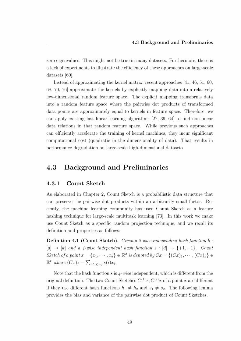
4.3 Background and Preliminaries

zero eigenvalues. This might not be true in many datasets. Furthermore, there is

a lack of experiments to illustrate the efficiency of these approaches on large-scale

datasets [60].

Instead of approximating the kernel matrix, recent approaches [41, 46, 51, 60,

68, 70, 76] approximate the kernels by explicitly mapping data into a relatively

low-dimensional random feature space. The explicit mapping transforms data

into a random feature space where the pairwise dot products of transformed

data points are approximately equal to kernels in feature space. Therefore, we

can apply existing fast linear learning algorithms [27, 39, 64] to find non-linear

data relations in that random feature space. While previous such approaches

can efficiently accelerate the training of kernel machines, they incur significant

computational cost (quadratic in the dimensionality of data). That results in

performance degradation on large-scale high-dimensional datasets.


4.3.1 Count Sketch

As elaborated in Chapter 2, Count Sketch is a probabilistic data structure that

can preserve the pairwise dot products within an arbitrarily small factor. Re-

cently, the machine learning community has used Count Sketch as a feature

hashing technique for large-scale multitask learning [73]. In this work we make

use Count Sketch as a specific random projection technique, and we recall its

definition and properties as follows:

Definition 4.1 (Count Sketch). Given a 2-wise independent hash function h :

[d] → [k] and a 4-wise independent hash function s : [d] → +1,−1. Count

Sketch of a point x = x1, · · · , xd ∈ Rd is denoted by Cx = (Cx)1, · · · , (Cx)k ∈Rk where (Cx)j =

∑i:h(i)=j s(i)xi.

Note that the hash function s is 4-wise independent, which is different from the

original definition. The two Count Sketches C(1)x,C(2)x of a point x are different

if they use different hash functions h1 6= h2 and s1 6= s2. The following lemma

provides the bias and variance of the pairwise dot product of Count Sketches.

49


Lemma 4.1. Given two points x, y ∈ Rd, we denote by Cx,Cy ∈ Rk the respec-

tive Count Sketches of x, y on the hash functions h : [d] → [k] and s : [d] →+1,−1, we have

E[〈Cx,Cy〉] = 〈x, y〉 ,

Var[〈Cx,Cy〉] =1

k

(∑i 6=j

x2i y

2j +

∑i 6=j

xiyixjyj

).

Proof. See Appendix B.

We derive an upper bound of variance of any pairwise dot product of Count

Sketches as follows:

Lemma 4.2. Given two points x, y ∈ Rd, we denote by Cx,Cy ∈ Rk the respec-

tive Count Sketches of x, y on the same hash functions h, s.

Var[〈Cx,Cy〉] ≤ 1

k

(〈x, y〉2 + ‖x‖2 ‖y‖2) .

Proof. Given any two points x = x1, · · · , xd , y = y1, · · · , yd, we have:

‖x‖2‖y‖2 =∑i

x2i y

2i +

∑i 6=j

x2i y

2j ,

〈x, y〉2 =∑i

x2i y

2i +

∑i 6=j

xiyixjyj .

By Lemma 4.1, we have:

Var[〈Cx,Cy〉] =1

k

(∑i 6=j

x2i y

2j +

∑i 6=j

xiyixjyj

)

=1

k

(〈x, y〉2 + ‖x‖2 ‖y‖2)− 2

k

∑i

x2i y

2i

≤ 1

k

(〈x, y〉2 + ‖x‖2 ‖y‖2) .

50


It is worth noting that Count Sketch might provide low distortion on sparse

vectors. This is due to the fact that non-zero elements will always be hashed into

a cell of Count Sketch. In other words, they are retained after sketching with high

probability. In addition, Count Sketch requires O(nd) operations for n points in

d-dimensional space. Therefore, Count Sketch might provide better performance

than traditional random projections in applications dealing with sparse vectors.

4.3.2 Tensor Product

Given a vector x = x1, · · · , xd ∈ Rd, the 2-level tensor product or outer product

x(2) = x⊗ x is defined as follows:

x(2) = x⊗ x =

x1x1 x1x2 · · · x1xd

x2x1 x2x2 · · · x2xd...

.... . .

...

xdx1 xdx2 · · · xdxd

∈ Rd2 .

Given an integer p, we consider a p-level tensor product Ωp : Rd → Rdp given by

x→ x(p) = x⊗ · · ·⊗︸︷︷︸p times

x .

The following lemma justifies that tensor product is an explicit feature map-

ping for the homogeneous polynomial kernel.

Lemma 4.3. Given any pair of points x, y and an integer p, we have:

⟨x(p), y(p)

⟩= 〈x, y〉p .

Proof. See [62, Proposition 2.1].

By taking y = x on Lemma 4.3, we have:

51


Lemma 4.4. Given any point x and an integer p, we have:

‖x(p)‖2 = ‖x‖2p .

It is obvious that the tensor product requires dp dimensions to comprise the

polynomial feature space. Therefore, it fails for realistically sized applications.

4.4 Tensor Sketching Approach

As elaborated above, it is infeasible to directly perform any learning algorithm

in the polynomial feature space. In this section, we introduce an efficient ap-

proach to randomly project the images of data without ever computing their

coordinates in that polynomial feature space. The proposed approach runs in

O(np(d+D logD)) time for n training examples in d-dimensional space and D

random projections, and outputs unbiased estimators of the degree-p polynomial

kernel of any pair of data points.

4.4.1 The Convolution of Count Sketches

Recently, Pagh [57] has introduced a fast algorithm to compute Count Sketch of an

outer product of two vectors. Instead of directly computing the outer product, the

approach compresses these vectors into their Count Sketches and then computes

the Count Sketch of their outer product by those sketches. Due to the fact that

the outer product of two different Count Sketches can be efficiently computed by

the polynomial multiplication (using FFT), we can compute the Count Sketch of

an outer product of any two vectors in time near-linear in the dimensionality of

the sketches.

More precisely, given a vector x ∈ Rd, we denote by C(1)x,C(2)x ∈ RD its two

different Count Sketches using 2-wise independent hash functions h1, h2 : [d] →[D] and 4-wise independent hash functions s1, s2 : [d] → +1,−1. We consider

the outer product x⊗x ∈ Rd2 and its Count Sketch Cx(2) ∈ RD using independent

and decomposable hash functions H : [d2] → [D] and S : [d2] → +1,−1. We

52

4.4 Tensor Sketching Approach

decompose H and S as follows:

H(i, j) = h1(i) + h2(j) mod D and S(i, j) = s1(i)s2(j).

We note that the hash functions H and S are 2-wise and 4-wise independent,

respectively [59]. We then represent a Count Sketch in D-dimensional space as

a polynomial of degree D − 1 where each coordinate corresponds to one term

of the polynomial. For example, we consider two degree-(D − 1) polynomials

representing for C(1)x,C(2)x:

P (1)x (ω) =

d∑i=1

s1(i)xiωh1(i) and P (2)

x (ω) =d∑j=1

s2(j)xjωh2(j).

We can fast compute the degree-(D−1) polynomial for Cx(2) using hash functions

H and S:

Px(2)(ω) =d∑

i,j=1

S(i, j)xixjωH(i,j)

= FFT−1(FFT(P (1)x ) ∗ FFT(P (2)

x )),

where (∗) is the component-wise product operator and FFT uses D interpolation

points. In other words, the Count Sketch Cx(2) of x⊗x can be efficiently computed

by Count Sketches C(1)x,C(2)x in O(d+D logD) time.

Inspired by the fast convolution of Count Sketches, we are able to efficiently

compute the polynomial Px(p)(ω) for the Count Sketch in D-dimensional space,

Cx(p), of the tensor product x(p) of any point x ∈ Rd by using independent and

decomposable hash functions H : [dp] → [D] and S : [dp] → +1,−1. We

decompose H and S as follows:

H(i1, · · · , ip) =

p∑k=1

hk(ik) mod D,

S(i1, · · · , ip) =

p∏k=1

sk(ik),

53


Algorithm 5 Tensor Sketching(S, p,D)

Require: A dataset S of size n, the number of random features D and the degreeof polynomial kernel p

Ensure: Return Count Sketches of the point set S as a random feature mappingf for the polynomial kernel κ(x, y) = 〈x, y〉p

1: f(S)← ∅2: Pick p independent hash functions h1, · · · , hp : [d]→ [D], each from a 2-wise

independent family3: Pick p independent hash functions s1, · · · , sp : [d] → +1,−1, each from a

4-wise independent family4: for each data point x ∈ S do5: Create p different Count Sketches: C(1)x, · · · , C(p)x6: (C(1)x, · · · , C(p)x)← FFT(C(1)x, · · · , C(p)x)7: Obtain f(x) in frequency domain by the component-wise multiplication

C(1)x ∗ · · · ∗ C(p)x8: f(x)← FFT−1(f(x))9: Insert f(x) into f(S)

10: end for11: return Return f(S)

where h1, · · · , hp : [d]→ [D] and s1, · · · , sp : [d]→ +1,−1 are chosen indepen-

dently from 2-wise and 4-wise independent family, respectively.

The proposed approach works in O(p(d+D logD)) time by using 2p different

and independent hash functions as elaborated above. This idea motivates the

intuition for Tensor Sketching approach to approximate polynomial kernels.

4.4.2 Tensor Sketching Approach

We exploit the fast computation of Count Sketches on tensor domains to in-

troduce an efficient algorithm for approximating the polynomial kernel κ(x, y) =

(〈x, y〉 + c)p, for an integer p and c ≥ 0. It is obvious that we can avoid the

constant c by adding an extra dimension of value√c to all data points. So, for

simplicity, we solely consider the homogeneous polynomial kernel κ(x, y) = 〈x, y〉p

for the proposed algorithm and theoretical analysis.

For each point x ∈ S ⊂ Rd, Tensor Sketching returns the Count Sketch of size

D of the tensor product x(p) as random feature maps in RD for the polynomial

54

4.5 Error Analysis

kernel. The pseudo-code in Algorithm 5 shows how Tensor Sketching works. We

maintain 2p independent hash functions h1, · · · , hp and s1, · · · , sp (lines 2 - 3).

For each point x, we create p different Count Sketches of size D using these 2p

different and independent hash functions (line 5). We then compute the Count

Sketch of x(p) by the usage of polynomial multiplication (using FFT) (lines 6-

8). As a result, we have obtained a random feature mapping f which provides

unbiased estimators for the polynomial kernel.

Now, we analyze the complexity of Tensor Sketching. It requires O(pd logD)

space usage to store 2p hash functions. For each point, the running time of

computing the Count Sketch of its p-level tensor product is O(pd+ pD logD)

due to applying FFT. Therefore, the total running time of Tensor Sketching is

O(np(d+D logD)). To increase the accuracy of estimates, we choose D = O(d);

therefore, we need O(npd log d) operations compared to O(nd2) of the previous

approaches [41, 60].

4.5 Error Analysis

In this section we analyze the precision of estimate of the kernel κ(x, y) = 〈x, y〉p,where x, y ∈ Rd and p is an integer, showing bounds on the number of random

features (D) to achieve a given absolute or relative precision ε. It is worth noting

that the previous approaches [41, 51, 60, 68] only introduced bounds of an absolute

error estimate. Often, however, the kernel has small value and a good absolute

error approximation is typically a poor relative error estimate. Large errors of

estimate might result in either performance degradation or negligible reduction

in computational cost.

4.5.1 Relative Error Bound

In contrast to the previous techniques, our approach can be viewed as a specific

random projection technique applied to images of data in the explicit polynomial

feature space. In fact, Tensor Sketching maintains random projections of images

of data in the feature space via independent hash functions of Count Sketches.

Therefore, its estimators are unbiased and have tight error bounds.

55


Given two points x, y ∈ Rd, we denote by Cx(p), Cy(p) ∈ RD the Count

Sketches of x(p), y(p) ∈ Rdp , respectively. Lemma 4.3 and 4.4 guarantee that

⟨x(p), y(p)

⟩= 〈x, y〉p , ‖x(p)‖ = ‖x‖p, ‖y(p)‖ = ‖y‖p .

So applying Lemma 4.1 and 4.2, we have:

Lemma 4.5.

E[⟨Cx(p), Cy(p)

⟩]= 〈x, y〉p ,

Var[⟨Cx(p), Cy(p)

⟩]≤ 1

D

(〈x, y〉2p + ‖x‖2p ‖y‖2p) .

While previous works on random feature mappings do not provide bounds

on the variance of estimates, the variance of our estimate can be bounded. We

make use Chebyshev’s inequality to bound the relative error, which depends on

the cosine of the angle θxy between x and y.

Lemma 4.6.

P[∣∣⟨Cx(p), Cy(p)

⟩− 〈x, y〉p

∣∣ ≥ ε 〈x, y〉p]≤ 2

Dε2

(1

cos θxy

)2p

.

Proof. Consider the random variable X =⟨Cx(p), Cy(p)

⟩, Chebyshev’s inequality

guarantees that:

P[|X − E[X]| ≥ εE[X]] ≤ Var[X]

ε2E[X]2

≤ 1

Dε2

〈x, y〉2p + ‖x‖2p ‖y‖2p

〈x, y〉2p

=1

Dε2

(1

(cos θxy)2p + 1

)≤ 2

Dε2

(1

cos θxy

)2p

.

It is obvious that we need more random features to approximate polynomial

kernels of large degree p. In addition, the relative error depends on the pairwise

angles of data points. So we have to use large D for almost orthogonal data

points to achieve a good approximation.

56

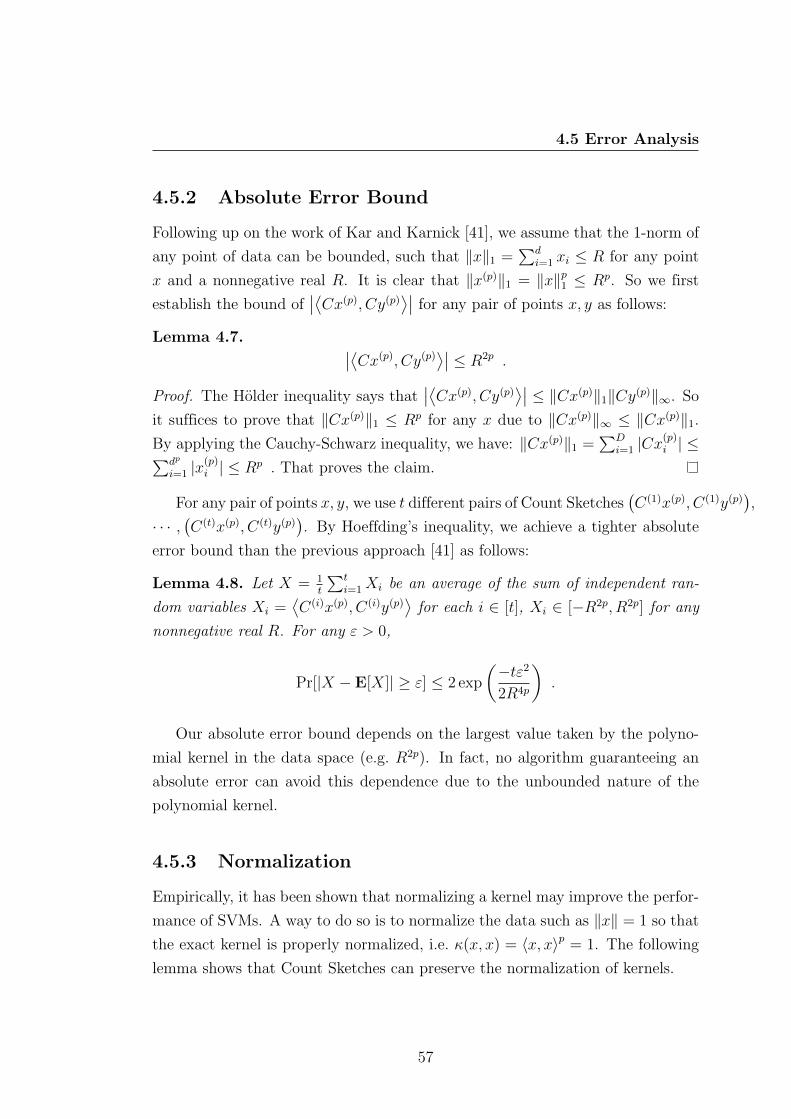
4.5 Error Analysis

4.5.2 Absolute Error Bound

Following up on the work of Kar and Karnick [41], we assume that the 1-norm of

any point of data can be bounded, such that ‖x‖1 =∑d

i=1 xi ≤ R for any point

x and a nonnegative real R. It is clear that ‖x(p)‖1 = ‖x‖p1 ≤ Rp. So we first

establish the bound of∣∣⟨Cx(p), Cy(p)

⟩∣∣ for any pair of points x, y as follows:

Lemma 4.7. ∣∣⟨Cx(p), Cy(p)⟩∣∣ ≤ R2p .

Proof. The Holder inequality says that∣∣⟨Cx(p), Cy(p)

⟩∣∣ ≤ ‖Cx(p)‖1‖Cy(p)‖∞. Soit suffices to prove that ‖Cx(p)‖1 ≤ Rp for any x due to ‖Cx(p)‖∞ ≤ ‖Cx(p)‖1.

By applying the Cauchy-Schwarz inequality, we have: ‖Cx(p)‖1 =∑D

i=1 |Cx(p)i | ≤∑dp

i=1 |x(p)i | ≤ Rp . That proves the claim.

For any pair of points x, y, we use t different pairs of Count Sketches(C(1)x(p), C(1)y(p)

),

· · · ,(C(t)x(p), C(t)y(p)

). By Hoeffding’s inequality, we achieve a tighter absolute

error bound than the previous approach [41] as follows:

Lemma 4.8. Let X = 1t

∑ti=1Xi be an average of the sum of independent ran-

dom variables Xi =⟨C(i)x(p), C(i)y(p)

⟩for each i ∈ [t], Xi ∈ [−R2p, R2p] for any

nonnegative real R. For any ε > 0,

Pr[|X − E[X]| ≥ ε] ≤ 2 exp

(−tε2

2R4p

).

Our absolute error bound depends on the largest value taken by the polyno-

mial kernel in the data space (e.g. R2p). In fact, no algorithm guaranteeing an

absolute error can avoid this dependence due to the unbounded nature of the

polynomial kernel.

4.5.3 Normalization

Empirically, it has been shown that normalizing a kernel may improve the perfor-

mance of SVMs. A way to do so is to normalize the data such as ‖x‖ = 1 so that

the exact kernel is properly normalized, i.e. κ(x, x) = 〈x, x〉p = 1. The following

lemma shows that Count Sketches can preserve the normalization of kernels.

57


Lemma 4.9. Given fixed constants ε, δ < 1 and a point x such that ‖x‖ = 1, we

denote by Cx(p) ∈ RD the Count Sketch of x(p). If ‖x(p)‖∞ ≤ ε

18√

log (1/δ) log (D/δ)

and D ≥ 72 log (1/δ)/ε2, we have that

Pr[∣∣⟨Cx(p), Cx(p)

⟩− 1∣∣ ≥ ε

]≤ 2δ.

Proof. See [73, Appendix B].

It is obvious that our kernel approximation can maintain the normalization of

kernels within an arbitrarily small factor. In contrast, the Maclaurin expansion

based approach [41] does not satisfy this property.

4.6 Experimental Results

We implemented random feature mappings in Matlab-7.11.0 and conducted ex-

periments in a 2.67 GHz core i7 Windows platform with 3GB of RAM. We com-

pared the performance of random feature mappings, including Tensor Sketching

(TS) and Random Maclaurin (RM) [41] with non-linear SVMs on 4 real world

datasets: Adult [29], Mnist [47], Gisette [15], and Covertype1 [29]. We used

LIBSVM-3.14 [15] for non-linear kernels and LIBLINEAR-1.92 [27] for random

feature mappings for classification task. All averages and standard deviations are

over 5 runs of the algorithms.


This subsection presents the accuracy experiments to evaluate the reliability of

our estimation algorithm. We carried out experiments to compare the accuracy

of estimators based on the number of random features (D) on two random feature

mappings: Tensor Sketching (TS) and Random Maclaurin (RM). We measured

the relative error of the approximation of the homogeneous and inhomogeneous

polynomial kernels of degree p = 2, 3, 4. We took D in ranges [500, 3000] and

1We sample 100,000 points for Covertype datasets due to the limit of RAM

58


500 1000 1500 2000 2500 30000.1

0.2

0.3

0.4

0.5

0.6

0.7

0.8

0.9

Number of random features (D)

Rel

ativ

e er

ror

(ε)

TS, κ = <x,y>2

TS, κ = (1 + <x,y>)2

RM, κ = <x,y>2

RM, κ = (1 + <x,y>)2

500 1000 1500 2000 2500 30000

1

2

3

4

5

Number of random features (D)R

elat

ive

erro

r (ε

)

TS, κ = <x,y>3

TS, κ = (1 + <x,y>)3

RM, κ = <x,y>3

RM, κ = (1 + <x,y>)3

500 1000 1500 2000 2500 30000

2

4

6

8

10

12


Rel

ativ

e er

ror

(ε)

TS, κ = <x,y>4

TS, κ = (1 + <x,y>)4

RM, κ = <x,y>4

RM, κ = (1 + <x,y>)4

Figure 4.1: Comparison of relative errors between Tensor Sketching (TS) andRandom Maclaurin (RM) estimators on the Adult dataset (n = 48,842, d = 123)using different polynomial kernels. (Figures best viewed in color.)

conducted experiments on Adult dataset with size n = 48, 842 and dimensionality

d = 123. Figure 4.1 displays the relative error (ε) from expectation of the two

approaches on different polynomial kernels.

It is obvious that TS provides a smaller error than the RM approach on

those polynomial kernels. The difference is most dramatic on the homogeneous

kernels because of the use of Rademacher vectors ωi ∈ +1,−1d in RM. In fact,

it estimates 〈x, y〉p as∏p

i=1 〈ωi, x〉∏p

i=1 〈ωi, y〉, which incurs very large variance,

especially for large p. Due to the fact that we have to normalize data before

applying any kernel method, RM gives small error on inhomogeneous kernels. In

this case, the value of Maclaurin expansion concentrates on some low order terms

that have small variance of estimate. When the accuracy of kernel machines

depends on higher order terms, RM either suffers from low accuracy or needs

large D due to large variance of estimate. In contrast, TS is a specific random

projection in the polynomial feature space. So it greatly outperforms RM and

does not require a large number of random features to achieve a small error. For

example, on the inhomogeneous kernels, TS only needs D = 500 to achieve ε < 1

while RM requires more than 3000 random features.

4.6.2 Efficiency

This subsection compares the random feature construction time of the two ap-

proaches, TS and RM, on two large high-dimensional datasets: Adult (d = 123)

59


0 500 1000 1500 2000 2500 3000 3500 40000

5

10

15

20

25

30

35


(a) CPU Time (s) on Adult and Mnist datasets

Tim

e (s

)

TS, Adult (d = 123)TS, Mnist (d = 780)RM, Adult (d = 123)RM, Mnist (d = 780)

0 500 1000 1500 2000 2500 3000 3500 4000 4500 50000

10

20

30

40

50

60

70


(b) CPU Time (s) on synthetic dataset

Tim

e (s

)

TS, Synthetic (d = D)RM, Synthetic (d = D)

Figure 4.2: Comparison of CPU time (s) between Tensor Sketching (TS) andRandom Maclaurin (RM) approaches on 3 datasets: (a) Adult (d = 123) andMnist (d = 780); (b) Synthetic (d = D) using κ = (1 + 〈x, y〉)4. (Figures bestviewed in color.)

and Mnist (d = 780). As analyzed above, TS requires O(np(d+D logD)) time

while RM demands O(ndD) time and much randomness. It is obvious that the

running time of TS is faster and less dependent on the original dimensionality of

data, a very desirable property since random feature mapping often contributes a

significant computational cost in training large-scale high-dimensional datasets.

Figure 4.2.a shows the CPU time requirements in seconds of the two ap-

proaches on the kernel κ = (1 + 〈x, y〉)4 when varying the number of random fea-

tures D in ranges [0, 4000] and fixing the number of training samples n = 10, 000.

It is clear that the running time of TS approach is almost independent from the

dimensionality of data d when using large D. On both Adult (d = 123) and

Mnist (d = 779) datasets, TS approach scales well when increasing D compared

to RM on Adult dataset. In contrast, RM shows a linear dependence with d,

as depicted on Mnist dataset (d = 780). When the dataset (e.g. Mnist) has a

smooth decision boundary, RM feature construction time dominates the training

time. This property might limit the use of RM.

When the dimensionality of data d increases, we need to increase the number

of random features D = O(d) to boost the accuracy. Figure 4.2.b demonstrates a

quadratic running time of RM in terms of dimensionality of data on the synthetic

60


dataset with setting d = D and n = 10, 000. This means that RM will be a

bottleneck of kernel machines on high-dimensional datasets. The next section

will show a significant domination of RM feature mapping when training on the

Gisette dataset (d = 5000).

4.6.3 Scalability

In this experiment, we compare the performance of random feature mappings

(TS, RM) along with LIBLINEAR [27] and non-linear kernel mapping along with

LIBSVM [15] for classification tasks on 4 large-scale datasets. We measured the

training accuracy and time of these approaches on a variety of polynomial kernels.

We note that training time of random feature mapping approaches include time

for feature construction and linear SVMs training.

Figure 4.3 and 4.4 demonstrate a comparison of accuracy between TS, RM and

non-linear SVMs on degree-2 polynomial kernels. The results impressively show

that TS provides higher accuracy than RM on 4 datasets. The most dramatic

difference is on the homogeneous kernels due to large error of estimate of RM.

Moreover, the accuracy of TS converges faster than RM to that of non-linear

kernels when increasing the number of random features D. RM even decreases

the accuracy on Gisette dataset because it requires a significantly large number

of random features for approximating higher order terms of Maclaurin expansion

well.

Figure 4.5 shows the CPU time requirements in seconds of the two approaches

in training linear SVMs using LIB-LINEAR on the kernel κ = (1 + 〈x, y〉)2. It is

obvious that TS provides performance benefits on high-dimensional datasets, such

as Mnist and Gisette. On Covertype and Adult datasets, RM is slightly faster

than TS. This is because RM generates more features for the low order terms of

Maclaurin expansion which do not require high computational cost. When p is

large, TS significantly outperforms RM, as illustrated in Table 4.1 and 4.2.

It is obvious that RM performs quite poorly on homogeneous kernels on the 4

datasets. Due to the large error of estimate in homogeneous kernels, RM provides

low accuracy on 4 datasets, especially in the kernel κ = 〈x, y〉4. In fact, the large

error of estimate produces meaningless results of training linear SVMs (e.g. 41.45

61


100 200 300 400 50055

60

65

70

75

80


(a) Covertype

Acc

urac

y (%

)

κ + LIBSVMTS + LIBLINEARRM + LIBLINEAR

100 200 300 400 50070

75

80

85


(b) Adult

Acc

urac

y (%

)


600 700 800 900 100070

75

80

85

90

95

100


(c) Mnist

Acc

urac

y (%

)


1000 2000 3000 4000 500080

85

90

95

100


(d) Gisette

Acc

urac

y (%

)


Figure 4.3: Comparison of accuracy of Tensor Sketching (TS), Random Maclaurin(RM) with LIBLINEAR and non-linear kernels with LIBSVM on 4 datasets withthe homogeneous kernel κ = 〈x, y〉2. (Figures best viewed in color.)

% of accuracy on the Mnist dataset). In contrast, TS shows stronger results

than both RM and non-linear SVMs because it requires rather small time for

feature construction and linear SVMs training while obtaining similar accuracy.

TS performs exceptionally well on datasets of non-smooth decision boundaries,

including Covertype and Adult, where it can achieve speed-ups of 50 and 1600

times, respectively, compared to non-linear SVMs on the kernel κ = (1 + 〈x, y〉)4.

62


100 200 300 400 50060

65

70

75

80


(a) Covertype

Acc

urac

y (%

)


100 200 300 400 50070

75

80

85


(b) AdultA

ccur

acy

(%)


600 700 800 900 100080

85

90

95

100


(c) Mnist

Acc

urac

y (%

)


1000 2000 3000 4000 500080

85

90

95

100


(d) Gisette

Acc

urac

y (%

)


Figure 4.4: Comparison of accuracy of Tensor Sketching (TS), Random Maclaurin(RM) with LIBLINEAR and non-linear kernels with LIBSVM on 4 datasets withthe inhomogeneous kernel κ = (1 + 〈x, y〉)2. (Figures best viewed in color.)

RM works better on inhomogeneous polynomial kernels because the value of

Maclaurin expansion concentrates on some low order terms. However it suffers

from large computational cost of random mapping in high-dimensional datasets

(e.g. Gisette and Mnist). Because these datasets have smooth decision bound-

aries, their training time is dominated by the random feature construction time.

So RM gives similar performance to non-linear SVMs on the Gisette dataset.

63


100 200 300 400 5000

20

40

60

80

100

120


(a) Covertype

Tim

e (s

)

TS + LIBLINEARRM + LIBLINEAR

100 200 300 400 500 100 200 300 4001

2

3

4

5

6

7

8

9


(b) Adult

Tim

e (s

)


600 700 800 900 100040

60

80

100

120

140

160

180


(c) Mnist

Tim

e (s

)


1000 2000 3000 4000 50000

10

20

30

40

50

60

70


(d) Gisette

Tim

e (s

)


Figure 4.5: Comparison of training time between Tensor Sketching (TS) andRandom Maclaurin (RM) with LIBLINEAR on 4 datasets with the inhomogeneouspolynomial kernel κ = (1 + 〈x, y〉)2. (Figures best viewed in color.)

When RM suffers from large error of estimate, it can influence the smoothness of

decision boundaries of linear SVMs algorithm and therefore require more train-

ing time. This explains the inefficiency of RM compared to non-linear SVMs on

Mnist dataset on the kernel κ = (1 + 〈x, y〉)4.

In contrast, the TS approach gives more stable and better performance than

RM and non-linear SVMs approaches on 4 datasets. In particular, it has a slightly

lower accuracy but runs much faster than non-linear SVMs. It not only achieves

higher accuracy (up to 7%), but also runs faster (up to 13 times) than RM on

the Mnist and Gisette datasets. Table 4.3 shows the speedup of TS compared to

64


Table 4.1: Comparison of Tensor Sketching (TS), Random Maclaurin (RM)feature mappings with LIBLINEAR and non-linear kernels with LIBSVM on 2datasets (Covertype and Mnist) on many polynomial kernels.

(a) Covertype (n = 100,000, d = 54, D = 500)

Kernel κ+libsvm TS+LIBLINEAR RM+LIBLINEAR

〈x, y〉2 79.73% 78.87±0.06% 72.58±1.46%11.3 mins 1.6 mins 3.7 secs

(1 + 〈x, y〉)2 79.73% 78.90±0.12% 75.96±0.45%11.5 mins 1.7 mins 0.8 mins

〈x, y〉4 84.01% 79.39±0.13% 58.55±2.75%1 hour 1.6 mins 3.3 secs

(1 + 〈x, y〉)4 84.20% 79.36±0.19% 76.76±0.42%1.5 hours 1.8 mins 1.6 mins

(b) Mnist (n = 60,000, d = 780, D = 1000)


〈x, y〉2 97.92% 95.81±0.08% 86.00±1.12%4.7 mins 1.3 mins 0.5 mins

(1 + 〈x, y〉)2 97.93% 95.84±0.10% 92.76±0.08%4.7 mins 1.3 mins 2.7 mins

〈x, y〉4 97.17% 92.49±0.22% 41.45±4.81%5 mins 2.1 mins 0.5 mins

(1 + 〈x, y〉)4 97.31% 92.44±0.04% 90.07±0.65%5 mins 2.1 mins 17.2 mins

RM and non-linear SVMs on 4 datasets on the kernel κ = (1 + 〈x, y〉)4.

The TS random mapping does not show any speedup on low-dimensional

datasets (e.g. Covertype, Adult) compared to RM, except for achieving smaller

error. However, TS runs 8 times faster than RM in training the Adult dataset

due to smaller estimation error. For high-dimensional datasets (e.g. Mnist and

Gisette), TS shows speedup on both random mapping and training time. Com-

pared to non-linear kernels, TS achieves significant speedup on Adult and Cover-

type which have non-smooth decision boundaries.

65


Table 4.2: Comparison of Tensor Sketching (TS), Random Maclaurin (RM)feature mappings with LIBLINEAR and non-linear kernels with LIBSVM on 2datasets (Adult and Gisette) on many polynomial kernels.

(a) Adult (n = 48,842, d = 123, D = 200)


〈x, y〉2 84.33% 84.33±0.12% 77.85±1.32%0.5 hours 3.6 secs < 1 sec

(1 + 〈x, y〉)2 84.34% 84.51±0.07% 84.42±0.10%0.5 hours 3.8 secs 3.4 secs

〈x, y〉4 79.34% 81.09±0.63% 58.04±2.37%2 hours 4.3 secs < 1 sec

(1 + 〈x, y〉)4 79.31% 81.89±0.24% 84.04±0.46%2 hours 4.5 secs 14.8 secs

(b) Gisette (n = 7000, d = 5000, D = 5000)


〈x, y〉2 97.54% 96.46±0.17% 90.40±0.79%1.4 mins 10.6 secs 1 min

(1 + 〈x, y〉)2 97.54% 96.23±0.14% 90.38±0.56%1.4 mins 10.6 secs 1.1 mins

〈x, y〉4 97.91% 95.11±0.15% 78.89±0.68%1.8 mins 13.6 secs 1.5 mins

(1 + 〈x, y〉)4 97.91% 95.21±0.33% 88.86±0.57%1.8 mins 13.5 secs 2.9 mins

Table 4.3: Speedup of Tensor Sketching compared to Random Maclaurin andnon-linear SVMs on κ = (1 + 〈x, y〉)4.

DatasetsRandom Maclaurin

κ + libsvmMapping Training

Adult (D = 200) __ 8× 1600×Covertype (D = 500) __ __ 50×Mnist (D = 1000) 2× 9× 2×Gisette (D = 5000) 9× 25× 8×

66


Table 4.4: Comparison of Tensor Sketching and Random Maclaurin with H0/1on κ = (1 + 〈x, y〉)4.

Datasets Tensor SketchingRandom Maclaurin

with H0/1Adult 81.89±0.24% 84.79±0.09%

D = 200 4.5 secs 5.7 secsCovertype 79.36±0.19% 78.88±0.12%D = 500 1.8 mins 2.2 minsMnist 92.44±0.04% 89.19±0.74%

D = 1000 2.1 mins 7.8 mins

4.6.4 Comparison with Heuristic H0/1

In the previous work, the authors [41] introduce a heuristic named H0/1 for

fast training. Due to the fact that we have to normalize data before apply-

ing any SVM-based learning algorithms, the value of Maclaurin expansion often

concentrates on the low order terms. Therefore, we can precompute the first

and second terms of the Maclaurin expansion to achieve higher accuracy. For

example, consider a Maclaurin expansion of a degree-4 polynomial kernel as fol-

lows: κ = (1 + 〈x, y〉)4 = 1 + 4 〈x, y〉 + 6 〈x, y〉2 + 4 〈x, y〉3 + 〈x, y〉4 . We can

easily compute 1 + 4 〈x, y〉 in advance and use D′ random features to estimate

6 〈x, y〉2 +4 〈x, y〉3 +〈x, y〉4. This means that H0/1 needs D = d+D′ random fea-

tures and is able to achieve higher accuracy due to the use of D′ random features

for approximating higher order terms.

However, H0/1 shows some disadvantages: (1) it cannot be used for homoge-

neous kernels; (2) it is not a dimensionality reduction technique because of using

d + D′ random features and (3) H0/1 requires longer feature construction times

due to the use of more randomness. When d is large, the feature construction

time is even larger and often dominates the training time. Table 4.4 shows the

comparison between Tensor Sketching and Random Maclaurin with H0/1. Note

that we do not use H0/1 on the Gisette dataset because of the large computational

cost of random feature construction.

Although RM with H0/1 can offer better accuracy than plain RM, its accuracy

is still lower than TS, except on the Adult dataset. In fact, the Adult dataset

67


works well and achieves higher accuracy (84.92%) on the kernel κ = 1 + 4 〈x, y〉than with κ = (1 + 〈x, y〉)4 (79.31%). That explains why the accuracy of RM

with H0/1 is exceptionally high. Due to the use of more randomness, the feature

construction time of RM with H0/1 is much longer than TS on 3 datasets. In

general, H0/1 is only suitable for low-dimensional datasets and works well when

the value of polynomial kernel highly concentrates on the first and second terms

of Maclaurin expansion.

4.7 Conclusion

In this chapter we have introduced a fast and scalable randomized tensor prod-

uct technique for approximating polynomial kernels, accelerating the training

of kernel machines. By exploiting the connection between tensor product and

fast convolution of Count Sketches, our approximation algorithm works in time

O(n(d+D logD)) for n training samples in d-dimensional space and D random

features. We present a theoretical analysis of the quality of approximation to

gua-rantee the reliability of our estimation algorithm. We show empirically that

our approach achieves higher accuracy and often runs orders of magnitude faster

than the state-of-the-art approach on large-scale real-world datasets.

An interesting research direction is analyzing and evaluating Tensor Sketching

on other learning tasks, such as clustering [20] and multitask learning [73] on

large-scale datasets. We also intend to apply Tensor Sketching on other kernels

(e.g. Gaussian kernel, sigmoid kernel) by exploiting Taylor-series approximations

of these kernels. By applying Tensor Sketching on Taylor-series approximations,

we might achieve a substantial speedup in training these kernel machines.

68

Chapter 5

High Similarity Estimation

Estimating set similarity is a central problem in many computer applications. In

this chapter we introduce the Odd Sketch, a compact binary sketch for estimat-

ing the Jaccard similarity of two sets. The exclusive-or of two sketches equals the

sketch of the symmetric difference of the two sets. This means that Odd Sketches

provide a highly space-efficient estimator for sets of high similarity, which is rel-

evant in applications such as web duplicate detection, collaborative filtering, and

association rule learning. The method extends to weighted Jaccard similarity,

relevant e.g. for TF-IDF vector comparison.

We present a theoretical analysis of the quality of estimation to guarantee the

reliability of Odd Sketch-based estimators. Our experiments confirm this effi-

ciency, and demonstrate the efficiency of Odd Sketches in comparison with b-bit

minwise hashing schemes on association rule learning and web duplicate detection

tasks.

This work was published as an article, “Efficient Estimation for High

Similarities using Odd Sketches” in Proceedings of 23rd International World

Wide Web Conference (WWW), 2014.

69

5. HIGH SIMILARITY ESTIMATION

5.1 Introduction

Estimating set similarities is a fundamental problem in databases, machine learn-

ing, and information retrieval. Given the two sets, S1 and S2, where S1, S2 ⊆ Ω =

0, 1, . . . , D − 1, a challenge is how to quickly compute their Jaccard similarity

coefficient J , a normalized measure of set similarity:

J(S1,S2) =|S1 ∩ S2||S1 ∪ S2|

.

One can view large datasets of Web documents as collections of sets where

sets and set elements correspond to documents and document words/shingles,

respectively. Other examples are datasets encountered in recommender systems,

where users and items can be viewed as sets and set elements. Hence, set simi-

larity estimation is one of the key research challenges in many application areas,

such as web duplicate detection [12, 14, 34, 53], collaborate filtering [5, 22], and

association rule learning [21].

Many applications of set similarity arise in large-scale datasets. For instance,

a search engine needs to crawl and index billions of web-pages. Collaborative

filtering engines from sites such as Amazon or NetFlix have to deal with tens of

millions of users’ data. Performing similarity search over such large-scale datasets

is very time-consuming. If we are willing to accept an estimate of J it turns out

that it is possible to get by with much less computation and storage. But how

much better can it get? In this work we address the following question:

If each set S is summarized in a data structure D(S) of n bits, how precise an

estimate of J(S1, S2) is it possible to make based on D(S1) and D(S2)?

Our main finding is that existing solutions, while highly efficient in general, are

not optimal when J is close to 1. We present a novel solution, the Odd Sketch,

that yields improved precision in the high similarity regime.

Although the setting where J is close to 1 has not often been the primary focus

when studying similarity measures, there are many applications where this regime

is important. Consider a setting where the goal is not just to find a similar item,

but to provide a short list and ranking of the most similar items. For example, in

70

5.1 Introduction

the setting of document similarity, in a sufficiently rich environment there may be

hundreds of documents quite similar to another document, and the user wants to

see the top ten. For such applications, we require methods that are very accurate

for high similarity values J .

5.1.1 Minwise Hashing Schemes

Because minwise hashing is a building block of our approach, and because b-bit

minwise hashing is our primary alternative for comparison, we review both briefly.

Minwise Hashing

Minwise hashing is a powerful algorithmic technique to estimate set similari-

ties, originally proposed by Broder et al. [12, 13]. It was used to detect and

cluster similar documents in the early AltaVista search engine [14]. Since then,

the scheme has been applied successfully in a variety of applications, including

similarity search [12, 13, 14], association rule learning [21], compressing social net-

works [18], advertising diversification [33], tracking Web spam [67], web duplicate

detection [48], large-scale learning [49], and more [5, 8, 45].

We now briefly review Broder’s minwise hashing scheme. Given a random

permutation π : Ω 7→ Ω, the Jaccard similarity of S1 and S2 is

J(S1,S2) = Pr[min(π(S1)) = min(π(S2))].

Therefore we get an estimator for J by considering a sequence of permutations

π1, . . . , πk and storing the annotated minimum values (called “minhashes”).

S1 = (i,min(πi(S1))) | i = 1, . . . , k,

S2 = (i,min(πi(S2))) | i = 1, . . . , k.

We estimate J by the fraction J = |S1 ∩ S2|/k. This estimator is unbiased, and

by independence of the permutations it can be shown that Var[J ] = J(1−J)k

.

71


xxxxxxxxxxxxxxxxxxxxxxxxxxxxxxxxxxxxxxxxxxxxxxxxxxxxxxxxxxxxxxxxxxxxxxxxxxxxxxxxxxxxxxxxxxxxxxxxxxxxxxxxxxxxxxxxxxxxxxxxxxxxxxxxxxxxxxxxxxxxxxxxxxxxxxxxxxxxxxxxxxxxxxxxxxxxxxxxxxxxxx

Jn bits

b-bit(S1)

S1

xxxxxxxxxxxxxxxxxxxxxxxxxxxxxxxxxxxxxxxxxxxxxxxxxxxxxxxxxxxxxxxxxxxxxxxxxxxxxxxxxxxxxxxxxxxxxxxxxxxxxxxxxxxxxxxxxxxxxxxxxxxxxxxxxxxxxxxxxxxxxxxxxxxxxxxxxxxxxxxx

xxxxx

xxxxxxxxxxxxxxxx

xxxxxxxxxxxxxxxxxxxxxxxxxxxx

xx

S2

xxxxxxxxxxxxxxxxxxxxxxxxxxxxxxxxxxxxxxxxxxxxxxxxxxxxxxxxxxxxxxxxxxxxxxxxxxxxxxxxxxxxxxxxxxxxxxxxxxxxxxxxxxxxxxxxxxxxxxxxxxxxxxxxxxxxxxxxxxxxxxxxxxxxxxxxxxxxxxxxxxxxxxxxxxxxxxx

b-bit(S2)

(1-J)n bits

xxxxxxxxxxx xxxxxxxxxxxxxxxxxxxxxxxx

Different independent hash values

Same independent hash valuesxxxxxxxx

Figure 5.1: Illustration of the b-bit minwise hashing construction. Given a highJaccard similarity J and two minhashes S1, S2, we expect that |S1∩S2| = Jn (filledspace) and |S1∆S2| = 2(1− J)n (white space). Due to the same independent hashvalues in the filled space, the error of the b-bit scheme corresponds to the error ofthe estimate of |S1∆S2|. Inaccuracy in just a few bit positions in the white spacewill yield a large relative error of the estimate of J .

Observe that a minhash can be stored as an array of length k containing the

minimum for each i = 1, . . . , k. The hash value min(π(S)) in the minhash is

stored as an integer of typically 32 or 64 bits. That means that Broder’s scheme

might use 32k or 64k bits of memory to store k hash values for any set S.

b-bit Minwise Hashing

AtWWW’10 Li and Konig [48] proposed b-bit minwise hashing as a space-efficient

variant of Broder’s minwise hashing scheme. Instead of storing b = 32 or b = 64

bits for each permutation, this approach suggested using the lowest b bits. It

is based on the intuition that the same hash values give the same lowest b bits

whereas the different hash values give different lowest b bits with probability

1− 1/2b. Figure 5.1 shows how to construct b-bit minwise sketches.

Let minb(π(S)) denote the lowest b bits of the hash value min(π(S)). Then

72

5.1 Introduction

the b-bit minhash Sb1 is obtained from the standard minhash S1 by replacing min

by minb, reducing space usage to kb. An unbiased estimator J b for J(S1, S2) and

its variance can be computed as follows:

J b =|Sb1 ∩ Sb2|/k − 1/2b

1− 1/2b, Var[J b] =

1− Jk

(J +

1

2b − 1

).

However, when the Jaccard similarity is high it seems that the b-bit scheme

offers less information than it might be able to. As an extreme example, suppose

that we get the estimate J b = 1, i.e., all the bits of the two summaries are

identical. How confident can we be that J is indeed close to 1? For example,

even if we actually have J = 1− 2kit is quite likely that the two summaries will be

identical. Somehow, since the two summaries are so highly correlated, differences

of just a few bit positions will lead to very different conclusions on how close J

is to 1. Thus we might ask: Is it possible to do better, avoiding the limits on

accuracy that comes when summaries are highly correlated?

5.1.2 Our Contribution

In this work, we introduce the Odd Sketch, a compact binary sketch for estimating

the Jaccard similarity of two sets. This binary sketch is similar to a Bloom filter

with one hash function [26], constructed on the original minhashes with the “odd”

feature that the usual disjunction is replaced by an exclusive-or operation. That

is, we hash each element of the minhash into a bit-array data structure. (We

will refer to the hash function used for this as the “sketch hash function”.) Now,

instead of setting a bit to 1, we flip a bit according to the sketch hash value of

each element in the minhash. We apply the Odd Sketches to minhashes, which

means that the Odd Sketch records for each hash value whether it is mapped

to by an odd number of elements in the minhash. Figure 5.2 shows a high level

illustration of the construction of Odd Sketches.

A key feature of the Odd Sketch is that when we compute the exclusive-or of

two Odd Sketches, the result will be equal to the Odd Sketch of the symmetric

difference of the minhashes, i.e., the set of elements in one minhash but not the

other. This is because the contribution of all identical elements in the minhashes

73


n bits

odd(S1)

S1

xxxxxxxxxxxxxxxxxxxxxxxxxxxxxxxxxxxxxxxxxxxxxxxxxxxxxxxxxxxxxxxxxxxxxxxxxxxxxxxxxxxxxxxxxxxxxxxxxxxxxxxxxxxxxxxxxxxxxxxxxxxxxxxxxxxxxxxxxxxxxxxxxxxxxxxxxxxxxxxx

xxxx

S2

odd(S2)

xxxxxxxxxxxxxxxxxxxxxxxxxxxxxxxxxxx

x

1

xxxx

1

xxxx

h(x)h(x)

x'x''

1

h(x')

xxx

1

h(x'')

Different independent hash values

Same independent hash values

Figure 5.2: Illustration of the Odd Sketch construction. Odd Sketch starts witha 0s bit-vector of size n. We flip a bit according to each element of the minhashesS1 and S2. The contributions of elements in S1 ∩ S2 cancel out in the exclusive-orodd(S1)⊕ odd(S2), so Odd Sketches use all of the n bits to estimate the symmetricdifference size |S1∆S2|. This reduces the variance when J is close to 1.

cancel out. In turn, this means that we are able to base Odd Sketches of size

n on minhashes of size significantly above n whenever J is close to 1 and there

are many identical values in the minhashes, so that the variance induced by the

minhash step is reduced.

The technical difficulty is to provide a good estimator for the size of a set

based on its Odd Sketch. We provide a surprisingly simple, asymptotically pre-

cise expression for the expected fraction of 1s in an Odd Sketch, and show via

concentration around this expectation that the resulting estimator has good pre-

cision as long as the fraction of 1s is bounded away from 1/2.

We note that a similar approach has previously been used to estimate the

number of distinct elements in a stream, where the usual disjunction was used

instead of an exclusive-or operation [6]. One of our contributions is showing

that tracking the parity of the number of items that hash to a bucket is a useful

technique in the context of estimating the size of set differences (rather than the

74

5.2 Odd Sketches

size of sets).

5.2 Odd Sketches

5.2.1 Construction

The Odd Sketch is a simple, linear sketch of the indicator vector of a set S.

Concretely, the sketch consists of an array s of n > 2 bits. Let h : Ω 7→ [n] be a

hash function, which we assume here is fully random. In the Odd Sketch, which

we denote by odd(S), the ith bit is given by

si = ⊕x∈S

1h(x)=i ,

where 0 ≤ i < n. That is, si is the parity of the number of set items that hash

to the ith location.

To compute the sketch, we start with the zero bit vector of size n. Then we

evaluate h on each x ∈ S, and flip the bit sh(x) of the sketch, as shown in the

pseudo-code in Algorithm 6.

Algorithm 6 Odd Sketch(S, n)

Require: A set S ⊂ Ω and the size of sketch in bits n1: s← [0]n

2: Pick a random hash function h : Ω 7→ [n]3: for each set element x ∈ S do4: sh(x) = sh(x) ⊕ 15: end for6: return s

Because odd(S) records the parity of the number of elements that hash to a

location, it follows that the Odd Sketch of the symmetric set difference S1∆S2 is

the exclusive-or of the Odd Sketches odd(S1) and odd(S2).

Lemma 5.1. odd(S1)⊕ odd(S2) = odd(S1∆S2).

75


In the following section, we show how to estimate the size of a set from the

number of 1s in its Odd Sketch. By Lemma 5.1 we can use this to estimate

|S1∆S2| from the Odd Sketches of S1 and S2. If sets S1 and S2 are minhashes of

S1 and S2, then we can estimate the Jaccard similarity of original two sets from

the Odd Sketches of S1 and S2.

5.2.2 Estimation

Estimating a Set’s Size from Its Odd Sketch

Let m and n denote the size of set S and the size of odd(S) in bits, respectively.

Because our hash functions are fully random, we can think about the process of

constructing odd(S) as that of independently throwing m balls into n bins, and

storing as si the parity of the number of balls in bin i. We are interested in

generating an estimate m for m based on the observation of the number of odd

bins in odd(S). In the following we present two estimation approaches for the

estimate m. The first one is based on the Markov chain model and the second

one relies on the standard Poisson approximation to the balls and bins setting.

Both approaches yield the same estimate when n is sufficiently large.

Consider the parity of number of balls landing in any specific bin (say the first)

as a simple two-state Markov chain model. The first/second state corresponds

to the even/odd parity. The probability of changing states is 1/n. Let pi be the

probability that any specific bin has an odd number of balls after i balls have

been thrown. A simple induction based on Markov chains yields

pi =1− (1− 2/n)i

2.

It helps to now introduce some notation. Let Xi be a 0-1 random variable

corresponding to the parity of the number of balls that land in the ith bin after

throwing m balls, and let X =∑

iXi. We have shown that

E[X] = n1− (1− 2/n)m

2.

76

5.2 Odd Sketches

Hence, a seemingly reasonable approximation for m if we see z odd bins in the

sketch is to assume that z ≈ E[X], in which case

z ≈ n1− (1− 2/n)m

2,

and solving we obtain an estimate m by

m =ln (1− 2z/n)

ln (1− 2/n). (5.1)

This approximation is reasonable if X is sharply concentrated around its expec-

tation, which we show later.

The second estimation approach leverages the standard Poisson approxima-

tion to the balls and bins setting and provides a pratical estimate. That is, when

m balls are thrown into n bins, this is very approximately the same as indepen-

dently giving each bin a number of balls that is Poisson distributed with mean

µ = m/n. (We discuss this further below; also, see [54, Section 5.4].) Lemma 5.2

provides the relationship between the Poisson distribution with mean µ and the

parity of the distribution.

Lemma 5.2. (Schuster and Philippou [63]) Let Q be a random variable that has

Poisson distribution with mean µ. The probability p that Q is odd is (1−e−2µ)/2.

Proof. The probability that Q is odd is given by

p =∑

i odd

e−µµi

i!= e−µ

∑i odd

µi

i!

= e−µeµ − e−µ

2=

1− e−2µ

2.

Let Yi be the parity of the number of balls that land in the ith bin in the

setting where the number of balls are independently Poisson distributed with

mean µ = m/n in each bin, and let Y =∑

i Yi be the number of bins with an

77


odd number of balls. Then

E[Y ] = np = n1− e−2m/n

2.

Hence, a seemingly reasonable approximation for m if we see z odd bins in the

sketch is to assume that z ≈ E[Y ], in which case we obtain an estimate m as

m = −n2

ln (1− 2z/n) . (5.2)

Since the Yi are independent and identically distributed, standard Chernoff

bounds provide that z ≈ E[Y ] with high probability, as we clarify further below.

We note that when n is sufficiently large in practice, we have ln (1− 2/n) ≈ −2/n.

In this case, the estimate is approximately the estimate derived from equation 5.1.

Estimating Jaccard Similarity from Odd Sketches

Suppose we construct Odd Sketches odd(S1), odd(S2) from the minhashes S1 and

S2 derived from S1 and S2. Recall that, when we construct sets S1 and S2, if we

think of the sets as random variables before instantiating them, we have

E[|S1∆S2|] = 2k(1− J),

where k is the number of independent permutations and J is the Jaccard sim-

ilarity of S1 and S2. Moreover, |S1∆S2| should be closely concentrated around

its expectation, since each permutation independently gives a match with prob-

ability J . Once we have instantiated S1 and S2, given odd(S1) and odd(S2),

we can estimate |S1∆S2| for the S1 and S2 we derived, using equation 5.2. For

notational convenience we will think of odd(S1) and odd(S2) as the sets of bit

positions containing 1, which means that their exclusive-or corresponds exactly

to the symmetric difference. If we use ˆ|S1∆S2| to denote our estimate of |S1∆S2|,then

ˆ|S1∆S2| = −n

2ln(1− 2 |odd(S1)∆odd(S2)|/n).

78

5.2 Odd Sketches

Here |odd(S1)∆odd(S2)| refers to the number of 1s in the structure. Using ˆ|S1∆S2|as a proxy for E[|S1∆S2|], the Jaccard similarity can be estimated as follows:

Jodd = 1−ˆ|S1∆S2|2k

= 1 +n

4kln

(1− 2 |odd(S1)∆odd(S2)|

n

).

Both Odd Sketches and b-bit minwise hashing can be viewed as variations of

the original minwise hashing scheme that reduce the number of bits used. The

quality of their estimators is dependent on the quality of the original minwise

estimators. In practice, both Odd Sketches and b-bit minwise hashing need to

use more permutations but less storage space than the original minwise hashing

scheme.

5.2.3 Analysis

In the previous section, we assumed that the number of odd bins in our data

structure was closely concentrated around its expectation to justify various ap-

proximations. Here we justify this assumption. This is straightforward in the

Poisson setting where bin parities are independent; we show how to handle the

dependencies that exist in the balls-and-bins model. We also directly calculate

the variance of the number of odd bins for both the Poisson and balls-and-bins

setting.

Concentration

Recall our notation: we throw m = µn balls into n bins, so that the average

number of balls per bin is µ. We let Xi be the parity of the number of balls that

land in the ith bin and X =∑

iXi be the number of odd bins. Similarly, let Yi

be the parity of the number of balls that land in the ith bin in the setting where

the number of balls are independently Poisson-distributed, and let Y =∑

i Yi.

We show that X and Y are closely concentrated around their means.

79


We use the standard approach of passing to the setting where each bin obtains

independently a Poisson distributed number of balls with mean µ. This is justified

by, for example, [54, Corollary 5.9] where the following is shown:

Lemma 5.3. [Corollary 5.9 of [54]] Any event that takes placed with probability

p when each bin obtains an independently distributed Poisson number of balls with

mean µ takes place with probability at most pe√m when m = µn balls are thrown

into n bins.

Since Y is the sum of independent 0-1 random variables, applying a Chernoff

bound [54, Exercise 4.13] to Y yields

Pr(|Y − E[Y ]| ≥ εn) ≤ 2e−2nε2 .

Hence, from Lemma 5.3 we have

Pr(|X − E[Y ]| ≥ εn) ≤ (2e√m)e−2nε2 .

Denote by X = 1nX the fraction of bins with an odd number of balls. We find

Pr(|X − 1

nE[Y ]| ≥ ε) ≤ (2e

√m)e−2nε2 ,

Pr(|X − p| ≥ ε) ≤ (2e√m)e−2nε2 ,

where p =(1− e−2m/n

)/2. The true expected fraction of odd bins is E[X]/n =

1−(1−2/n)m

2, which differs from p by an o(1) amount.

Since m corresponds to the symmetric difference between two minhashes,

we have m ≤ 2k. Hence, by choosing n > cε−2 log k for some constant c, our

estimator closely concentrates around its mean with probability 1− k−ω(1).

Variance Bound

We note that the variance on the number of odd bins for the Poisson setting is

trivial to calculate, since the bins are independent. Letting p =(1− e−2m/n

)/2,

80

5.2 Odd Sketches

the standard result (on variance of biased coin flips) gives that the variance is

np(1− p).

For the balls and bins case there are dependencies among the bin loads that

make the variance calculation more difficult. Recall that pi is the probability that

any specific bin has an odd number of balls after i balls have been thrown, and

pi =1− (1− 2/n)i

2,

so each Xi = 1 with probability (1 − (1 − 2/n)m)/2. To calculate the variance,

we first calculate E[X2]; the standard expansion gives

E[X2] = E[(∑i

Xi)2]

=∑i

E[X2i ] + 2

∑i<j

E[XiXj]

=∑i

E[Xi] + 2∑i<j

E[XiXj].

where we have used the fact that (Xi)2 = Xi since Xi only takes on the values

0-1. The first summation is just E[X].

To calculate the second summation, by symmetry it suffices to consider a

specific pair of variables, say X1 and X2. We consider the total number of balls

that land in the combination of bins 1 and 2. If this number is odd, then clearly

X1X2 = 0. If this number is 0, then clearly X1X2 = 0. If this number is even, but

more than 0, then X1X2 = 1 with probability exactly 1/2. To see this, consider

the last ball that lands in either bin 1 or bin 2. One of these bins must have an

odd number of balls. If the new ball lands in the other bin, then both have an

odd number of balls; this happens with probability 1/2. It follows that E[X1X2]

is half the probability that bins 1 and 2 considered together obtain an even and

positive number of balls. As with the calculation for pi, a simple induction based

on the two-state Markov chain model shows that after i balls have been thrown,

the probability qi that the first two bins have an even number of balls greater

81


than 0 is

qi =1 + (1− 4/n)i − 2(1− 2/n)i

2.

Hence the second sum is(n

2

)1 + (1− 4/n)m − 2(1− 2/n)m

2.

The variance is then E[X2]− E[X]2, or

(n

2

)1 + (1− 4/n)m − 2(1− 2/n)m

2

+n(1− (1− 2/n)m)

2−(n(1− (1− 2/n)m)

2

)2

.

Simplifying, this is

n2 (1− 4/n)m − (1− 2/n)2m

4+ n

1− (1− 4/n)m

4.

While this is easily seen to be O(n2), the coefficient

(1− 4/n)m − (1− 2/n)2m

4

of the n2 term above is in fact O(1/n2) whenm = µn. (Note that both expressions

in the numerator converge to and are approximately e−4m/n. By examining the

asymptotics carefully one can show the coefficient isO(1/n2).) Hence the variance

here is also O(n). Indeed, the second term is

n1− (1− 4/n)m

4≈ n

1− e−4m/n

4= np(1− p),

which is the variance for the Poisson setting, and the first term is negative. Again,

by considering the asymptotic expansions carefully one obtains that the variance

in the Poisson case is larger than in the case where there are exactly m balls

thrown for large enough n, as one might naturally expect.

82

5.2 Odd Sketches

Accuracy of the Estimator

In the previous sections we bounded the variance and gave strong tail bounds

for the fraction z/n of 1s in an Odd Sketch. Recall that its expected value is

pm = 1−(1−2/n)m

2derived from the Markov chain and its practical estimate is

p = 1−e−2m/n

2derived from the Poisson approximation. What remains is to bound

the error resulting from applying the estimator from equation (5.2), repeated here

for convenience:

m = −n2

ln (1− 2z/n) .

Defining the function f(x) = −n2

ln(1− 2x), we have m = f(z/n). There are

two sources of inaccuracy: The first is that the estimator has a bias since the

expected number of 1s, npm = n1−(1−2/n)m

2, differs from the practical estimate

np = n1−e−2m/n

2. However, it can be confirmed by an easy computation that the

difference can be at most 1, so this is not significant.

The second, and more significant, source of error is that when z/n deviates

from its expectation pm, f(z/n) will deviate from f(pm). Informally, an if z/n

deviates from its expectation by ε, this will give an error of roughly f ′(z/n) ·ε, aslong as ε is small enough, where f ′(x) = n

1−2xis the derivative of f . It is clear that

a small error can be magnified significantly if z/n is close to 1/2, since f ′(x) goes

to infinity as x→ 1/2. Therefore we choose parameters such that p, the practical

estimate of z/n, is bounded away from 1/2 (p ≈ 0.3 gives the best results, as

we see when we discuss our experiments). By the results in section 5.2.3 this

means that with high probability (wrt. n) we will have z/n < 0.4 (say). As long

as this is the case, since f ′ is monotonely increasing, we have that the error is

bounded by f ′(0.4)|z/n − pm| = 5n. This bound is pessimistic, but shows that

the estimation error is (with high probability) proportional to the error in the

estimate of pm. In turn, this implies that the variance of the estimator is O(n).

5.2.4 Weighted Similarity

Odd Sketches work with any notion of similarity that can be transformed to Ham-

ming distance of two vectors. In particular, it works with any similarity measure

that can be captured using the probability that two minhashes are identical. For

83


example, the Jaccard similarity of two vectors v, w ∈ Rd with nonnegative entries

can be defined as:

J(v, w) =

∑i min(vi, wi)∑i max(vi, wi)

,

generalizing standard Jaccard similarity which corresponds to 0-1 vectors. Hash

functions that result in minhash equality with probability J(v, w) can be found

in [32, 38, 52].


We implemented b-bit minwise hashing and Odd Sketch in Matlab, and con-

ducted experiments on a 2.67 GHz Core i7 Windows machine with 3GB of RAM.

We compared the performance of b-bit minwise hashing and Odd Sketch on as-

sociation rule learning and web duplication detection tasks. All results are the

averages of 10 runs of the algorithms.

5.3.1 Parameter Setting

It is obvious that the performance of both b-bit minwise and Odd Sketch depends

on the number of independent permutations used in the original minwise hashing

scheme. The b-bit minwise scheme uses kb = n/b permutations where the storage

space is n bits and b ≥ 1 is the number of bits per permutation. Since larger kb

provides higher accuracy, setting b = 1 turns out to achieve the smallest variance,

as will be clear from our empirical evaluation.

In the Odd Sketch setting, the number of independent permutations kodd is

dependent on the sketch size n and the user-defined similarity threshold J0. Typ-

ically, we are interested in retrieving pairs of sets such that J > J0 (and perhaps

subject these pairs to additional filtering). Moreover, we want to choose kodd

as large as possible to reduce the error from the original minwise hashing step.

It seems difficult to mathematically establish the optimal way of choosing kodd,

but we conducted experiments that indicate that the smallest variance is achieved

when the exclusive-or of two odd sketches with similarity J0 contains around 30%

1s.

84


0.25 0.28 0.33 0.4 0.5 0.670.075

0.08

0.085

0.09

0.095

0.1

0.105

Ratio (α)

(a) J = 0.9, n = 500 − 1000

Ave

rage

MS

E

0.25 0.28 0.33 0.4 0.5 0.670.032

0.033

0.034

0.035

0.036

0.037

0.038

0.039

0.04

0.041

0.042

Ratio (α)

(b) n = 800, J = 0.75 − 0.95

Ave

rage

MS

E

Figure 5.3: Comparison of the average MSE on different ratios α on the syntheticdataset: (a) Fix J = 0.9 and change n = 500− 1000 bits; (b) Fix n = 800 bits andchange J = 0.75− 0.95.

Our estimator needs the fraction of 1s in odd(S1∆S2) to be smaller than 1/2.

If a fraction of more than 1/2 is observed this is (with high probability) a sign of

very low Jaccard similarity, so we may estimate J = 0. Recall that the process

of constructing odd(S1∆S2) corresponds to throwing |S1∆S2| balls into n bins.

It turns out that if we choose kodd such that |S1∆S2| ≈ n/2 we get the most

accurate estimate when similarity is around J . In other words, we choose the

parameter kodd such that the ratio α = 2kodd(1−J0)n

≈ 12.

We conducted experiments to evaluate this choice of ratio α. We compared the

mean square error (MSE, incorporating both variance and bias) of our estimator

Jodd for different ratios of α = 2kodd(1−J0)n

in [0.25, 1], and for different sketch sizes

n ∈ [500, 1000] bits. For each choice we found that α = 1/2 gave the smallest

observed MSE. Figure 5.3 displays the average MSE of Jodd, averaged over variety

of values of J and n. It illustrates that Odd Sketch achieves the highest accuracy

when using the ratio α = 0.5. So we can choose kodd = n4(1−J0)

given a threshold

J0. When we are interested in J0 ≥ 0.75, we can set kodd > n. This means

that Odd Sketch can use more independent permutations than b-bit schemes.

85


0.70 0.75 0.80 0.85 0.90 0.95 0.996

7

8

9

10

11

12

13

14

The Jaccard similarity (J)

(a) n = 512

−lo

g(M

SE

)

Oddb = 1b = 2b = 4

0.70 0.75 0.80 0.85 0.90 0.95 0.996

7

8

9

10

11

12

13

14


(b) n = 1024

−lo

g(M

SE

)

Oddb = 1b = 2b = 4

Figure 5.4: Comparison of the negative log of mean square error (MSE) of OddSketch and b-bit minwise hashing for different Jaccard similarity. In these exper-iments Odd Sketch used kodd = n

4(1−J) permutations, and b-bit minwise hashingused kb = n

b .

In fact, even for the inferior choice of kodd = n, Odd Sketch can achieve better

performance than 1-bit minwise hashing when J0 > 0.75.


This subsection shows experiments to further evaluate the accuracy of our esti-

mation algorithm. We carried out experiments to compare the accuracy of b-bit

minwise hashing and Odd Sketch. In the b-bit schemes, we set kb = n/b to achieve

a space usage of n bits. For the Odd Sketch, we set kodd = n4(1−J)

. We again mea-

sured the mean square error (MSE) of estimators of both approaches. We varied

n in 512, 1024 bits and conducted experiments on synthetic datasets. (But

note that since we apply hashing the outcome is independent of the particular set

elements, and we expect the same result on any real-life dataset.) This dataset

is very high-dimensional (D = 10, 000) and highly sparse (sparsity > 99.9%).

Figure 5.4 shows the negative log of MSE (− log (MSE)) of estimators of the

86


0.70 0.75 0.80 0.85 0.90 0.95 0.996

6.5

7

7.5

8

8.5

9

9.5

10

10.5

11

11.5


(a) n = 512

−lo

g(M

SE

)

Oddb = 1b = 2b = 4

0.70 0.75 0.80 0.85 0.90 0.95 0.996

6.5

7

7.5

8

8.5

9

9.5

10

10.5

11

11.5


(b) n = 1024

−lo

g(M

SE

)

Oddb = 1b = 2b = 4

Figure 5.5: Comparison of the negative log of mean square error (MSE) of OddSketch and b-bit minwise hashing for different Jaccard similarities. Here, OddSketch uses kodd = n, and b-bit minwise hashing uses kb = n

b permutations.

two approaches for different values J . We note that the MSE is always smaller

than 1 in our experiments, so larger − log (MSE) is better. For high Jaccard

similarities J ≥ 0.8, Odd Sketch provides a smaller error than the b-bit minwise

approach. The difference is more dramatic when J is very high because Odd

Sketch makes use of a larger number of independent permutations than the b-

bit minwise schemes. This figure also shows that the 1-bit scheme has superior

performance compared to the b-bit schemes for b > 1. We note that b-bit schemes

for b > 1 require additional bit-manipulation to pack b bits of hash values into

64-bit (or 32-bit) words. In contrast, both Odd Sketch and 1-bit schemes only

need the XOR and bit-counting operations to compare two summaries.

One might argue that Odd Sketch requires a more expensive preprocessing

step than b-bit minwise hashing due to the use of larger number of permutations

in the minwise hashing step. But even with kodd = n, where the hashing cost

is identical to that of 1-bit minwise hashing, Odd Sketch still provides better

accuracy when J > 0.75, as shown in Figure 5.5.

87


0.75 0.80 0.85 0.90 0.95 0.997

8

9

10

11

12

13

14


(a) Different k setting

−lo

g(M

SE

)

Oddb = 1/2

0.75 0.80 0.85 0.90 0.95 0.996

7

8

9

10

11

12

13


(b) Same k setting

−lo

g(M

SE

)

Oddb = 1/2

Figure 5.6: Comparison of the negative log of mean square error (MSE) of OddSketch and 1

2 -bit minwise hashing for different Jaccard similarities: (a) Differentnumber of permutations: kodd = n

4(1−J) and k 12

= 2n; (b) Same number of permu-tations: kodd = k 1

2= 2n.

When the target similarity is very high, the authors of b-bit minwise hashing

also discussed the idea of combining any 2 bits of a 1-bit minhash by XOR

operations to increase the amount of information in each bit. This approach is

called 12-bit minwise hashing, and similar to Odd Sketch has a nonlinear estimator.

The 12-bit scheme uses k 1

2= 2n permutations.

We carried out experiments to compare the mean square errors of estimators

of Odd Sketch and 12-bit minwise hashing, as shown in Figure 5.6. The figure

shows that Odd Sketch achieves a considerably smaller error than 12-bit minwise

hashing when J > 0.85 for both choices of k. It also shows that Odd Sketch with

the best choice of kodd provides higher accuracy than for kodd = 2n.

We conclude the accuracy evaluation of Odd Sketch by depicting the empir-

ical cumulative distribution function (cdf) of estimators. Figure 5.7 shows the

empirical cdfs of Odd Sketch, 1-bit scheme and 12-bit scheme on 10,000 estima-

88


0.85 0.86 0.87 0.88 0.89 0.9 0.91 0.92 0.93 0.94 0.950

0.1

0.2

0.3

0.4

0.5

0.6

0.7

0.8

0.9

1

Estimator of J

Cum

mul

ativ

e P

roba

bilit

y

Oddb = 1/2b = 1

Figure 5.7: Comparison of the empirical cumulative distribution function (cdf)of estimators based on Odd Sketch, 1-bit scheme, and 1

2 -bit scheme with J = 0.9.

tors of the Jaccard similarity J = 0.9. The slope of cdf of Odd Sketch is steeper

than that of 12-bit scheme and significantly steeper than that of 1-bit scheme.

This means that Odd Sketch provides superior performance compared to b-bit

minwise hashing when the target similarity is high.

5.3.3 Association Rule Learning

Cohen et al. [21] used minwise hashing to generate the candidate sets of high Jac-

card similarity in the context of learning pairwise associations. This subsection

compares the performance of Odd Sketch and b-bit schemes in this setting. Since

b = 1 provides the highest accuracy among b ≥ 1, we only used the 1-bit scheme

in our experiment. For a more clear comparison, we used the same number of per-

mutations for the two approaches. We measured the precision-recall ratio of both

approaches on detecting the pairwise items that have Jaccard similarity larger

89


100 200 300 400 5000.5

0.6

0.7

0.8

0.9

1

The size of sketch in bits (n)

(a) J0 = 0.9

Pre

cisi

on

Oddb = 1

100 200 300 400 5000.5

0.6

0.7

0.8

0.9

1


(b) J0 = 0.9

Rec

all

Oddb = 1

100 200 300 400 5000.5

0.6

0.7

0.8

0.9

1


(c) J0 = 0.8

Pre

cisi

on

Oddb = 1

100 200 300 400 5000.4

0.5

0.6

0.7

0.8

0.9

1


(d) J0 = 0.8

Rec

all

Oddb = 1

Figure 5.8: Comparison of the precision-recall ratio between Odd Sketches and1-bit scheme on the mushroom dataset.

than a threshold J0. We conducted experiments on the large public datasets1:

mushroom (N = 8124;D = 119) and connect (N = 67, 557;D = 127). Due to

the similar results on both datasets, we only report the representative results of

mushroom dataset here.

Figure 5.8 shows the precision-recall ratio of the Odd Sketch and the 1-bit

scheme. For the high target threshold J0 = 0.9, the Odd Sketch provides signif-

icantly higher precision and recall ratio (up to 10% better) than 1-bit minwise

hashing. For J0 = 0.8, the Odd Sketch is still better in precision but slightly

1http://fimi.ua.ac.be/data/

90


100 200 300 400 5000.5

0.55

0.6

0.65

0.7

0.75

0.8

0.85

0.9

0.95

1


(a) J0 = 0.9

Pre

cisi

on

Oddb = 1/2

100 200 300 400 5000.5

0.55

0.6

0.65

0.7

0.75

0.8

0.85

0.9

0.95

1


(b) J0 = 0.9

Rec

all

Oddb = 1/2

Figure 5.9: Comparison of the precision-recall ratio between Odd Sketches and12 -bit scheme on the mushroom dataset with J0 = 0.9.

worse in recall.

Figure 5.9 demonstrates the superiority of Odd Sketch compared to 12-bit

minwise hashing with respect to precision. The Odd Sketch achieved up to 20%

higher precision while providing similar recall.

5.3.4 Web Duplicate Detection

In this experiment, we compare the performance of the two approaches on web du-

plicate detection tasks on the bag of words dataset1. We picked three datasets, in-

cluding KOS blog entires (D = 6906;N = 3430), Enron Emails (D = 28, 102;N =

39, 861), and NYTimes articles (D = 102, 660;N = 300, 000). We computed all

pairwise Jaccard similarities among documents, and retrieved every pair with

J > J0. For the sake of comparison, we used the same number of permutations

and considered the thresholds J0 = 0.85 and J0 = 0.90. We again used the

precision-recall ratio as our standard measure.

1http://archive.ics.uci.edu/ml/datasets/Bag+of+Words

91


100 200 300 400 5000.75

0.8

0.85

0.9

0.95


(a) KOS blog entries

Pre

cisi

on

Oddb = 1

100 200 300 400 5000.75

0.8

0.85

0.9

0.95

1


(b) Enron Emails

Pre

cisi

on

Oddb = 1

100 200 300 400 5000.75

0.8

0.85

0.9

0.95

1


(c) NY Times articles

Pre

cisi

on

Oddb = 1

100 200 300 400 5000.4

0.5

0.6

0.7

0.8

0.9


(d) KOS blog entries

Rec

all

Oddb = 1

100 200 300 400 5000.75

0.8

0.85

0.9

0.95


(e) Enron Emails

Rec

all

Oddb = 1

100 200 300 400 5000.98

0.985

0.99

0.995

1


(f) NY Times articles

Rec

all

Oddb = 1

Figure 5.10: Comparison of the precision-recall ratio between Odd Sketches and1-bit minwise hashing with J0 = 0.85 on the three datasets: KOS blog entries,Enron Emails and NYTimes articles.

Figures 5.10 and 5.11 show the precision-recall ratio for the Odd Sketch and

1-bit minwise hashing on three datasets with J0 = 0.85 and J0 = 0.9, respectively.

The Odd Sketch obtains higher relative precision ratio or at least is comparable

to 1-bit scheme when J0 = 0.85. It achieves up to 7% and 1% higher than the

1-bit scheme on KOS blog entries and Enron Emails, respectively. For J0 =

0.9, the precision ratios are almost the same on three datasets. However, Odd

Sketch greatly outperforms in the recall ratio. The Odd Sketch’s relative recall is

approximately 15% higher than the 1-bit scheme on the KOS blog entries when

J0 = 0.85 and J0 = 0.9. The difference in relative recall is not significant on the

other datasets. These relative gaps are around 5% and less 1% on Enron Emails

and NYTimes articles, respectively.

Figure 5.12 shows the observed precision-recall graphs of the Odd Sketch and

the 12-bit scheme. We again set kodd = k1 = 2n for the sake of fair comparison.

Both approaches achieve very high precision (higher than 90%) on the three

datasets. The Odd Sketch still obtains higher precision than the 12-bit scheme

although the difference is not dramatic. The gap of both schemes in the recall

92

5.4 Conclusion

100 200 300 400 5000.75

0.8

0.85

0.9

0.95



Pre

cisi

on

Oddb = 1

100 200 300 400 5000.75

0.8

0.85

0.9

0.95

1


(b) Enron EmailsP

reci

sion

Oddb = 1

100 200 300 400 5000.75

0.8

0.85

0.9

0.95

1



Pre

cisi

on

Oddb = 1

100 200 300 400 5000.3

0.4

0.5

0.6

0.7

0.8

0.9



Rec

all

Oddb = 1

100 200 300 400 5000.75

0.8

0.85

0.9

0.95


(e) Enron Emails

Rec

all

Oddb = 1

100 200 300 400 5000.98

0.985

0.99

0.995

1



Rec

all

Oddb = 1

Figure 5.11: Comparison of the precision-recall ratio between Odd Sketches and1-bit minwise hashing with J0 = 0.9 on the three datasets: KOS blog entries, EnronEmails and NYTimes articles.

ratio is considerable on KOS blog entries and Enron Emails. The most dramatic

difference is around 4% when n = 200. On the NYTimes articles dataset, the

ratio curves of both schemes are overlapping when n ≥ 200.

5.4 Conclusion

In this chapter, we proposed the Odd Sketch, a compact binary sketch for esti-

mating the Jaccard similarity of two sets. By combining the minwise hashing

technique with a hash table where only the parity of the number of items hashed

to bucket is stored, Odd Sketches can be combined with just an exclusive-or op-

eration to allow a simple estimation of the Jaccard similarity that provides a

highly space-efficient solution, particularly for the high similarity regime. We

presented a theoretical analysis of the quality of estimate. Our experiments on

synthetic and real world datasets demonstrate the efficiency of Odd Sketches in

comparison with b-bit minwise hashing schemes on association rule learning and

93


100 200 300 400 5000.75

0.8

0.85

0.9

0.95



Pre

cisi

on

Oddb = 1/2

100 200 300 400 5000.85

0.9

0.95

1


(b) Enron Emails

Pre

cisi

on

Oddb = 1/2

100 200 300 400 5000.98

0.985

0.99

0.995

1



Pre

cisi

on

Oddb = 1/2

100 200 300 400 5000.5

0.6

0.7

0.8

0.9

1



Rec

all

Oddb = 1/2

100 200 300 400 5000.7

0.75

0.8

0.85

0.9

0.95

1


(e) Enron Emails

Rec

all

Oddb = 1/2

100 200 300 400 5000.9

0.92

0.94

0.96

0.98

1



Rec

all

Oddb = 1/2

Figure 5.12: Comparison of the precision-recall ratio between Odd Sketches and12 -bit minwise hashing with J0 = 0.9 on the three datasets: KOS blog entries,Enron Emails and NYTimes articles.

web duplicate detection tasks. We expect that there are many other additional

applications where Odd Sketches can be similarly applied.

94

Chapter 6

Conclusions

Big data analytics have been growing demands for not only novel platform sys-

tem architectures but also computational algorithms to address the fast-paced big

data needs. Designing and evaluating scalable and efficient algorithms that are

able to handle complex big data analysis tasks without excessive use of compu-

tational resources have become a major research topic in computer science fields,

such as data mining, machine learning, information retrieval, etc. Not surpris-

ingly, in a wide range of data-intensive applications, randomized algorithms are

substantially more efficient than the best known deterministic solutions. The use

of randomization often leads to simpler and faster algorithms with little or no loss

in performance. In addition, in most cases, the randomized algorithms can be or-

ganized to exploit parallel computing environments where existing deterministic

algorithms fail to run at all.

In the thesis, we continued the line of research on exploiting randomization

in big data analytics. We investigated the fundamental data analysis problems

including angle-based outlier detection, large-scale SVM classification and high

similarity estimation. We showed how to apply advanced randomized techniques,

e.g. sampling and sketching, to solve these fundamental tasks. By taking advan-

tage of benefits of randomized techniques, our proposed randomized algorithms

are very scalable, compact and fast solutions. The experiments on large-scale real

world data sets demonstrated the efficiency and scalability of our approaches on

95

6. CONCLUSIONS

such problems in large-scale data analysis. In short, the thesis is an exhibition of

the power of randomization in big data analytics.

In future we hope to exploit the power of randomization not only on the

algorithmic aspects but also on the platform system architectures for big data

analytics. That means that the designed randomized algorithms should fit well

into the MapReduce paradigm for massive scalability across hundreds or thou-

sands of servers in a Hadoop cluster. Therefore we can achieve significant parallel

and sequential speedups.

In closing, randomization not only plays an important role in algorithm design,

but also provides a powerful framework to address a wide range of data-intensive

applications in modern massive data set analysis.

96

Appendix A

CW Trick

We describe the pseudo-code of CW-trick to generate 4-wise independent random

variables. This trick will use the Mersenne prime PRIME = 231 − 1 to generate

4-wise independent random variable.

Algorithm 7 CW-trick(x, a, b, c, d, e)

Ensure: Return a 4-wise independent random variable1: h = hash31(hash31(hash31(hash31(x, a, b), x, c), x, d), x, e)2: h = h&PRIME3: return h

Algorithm 8 hash31(x, a, b)

Ensure: Return a 2-wise independent random variable1: h = a ∗ x+ b2: h = h+ h >> 313: return h&PRIME

97

A. CW TRICK

98

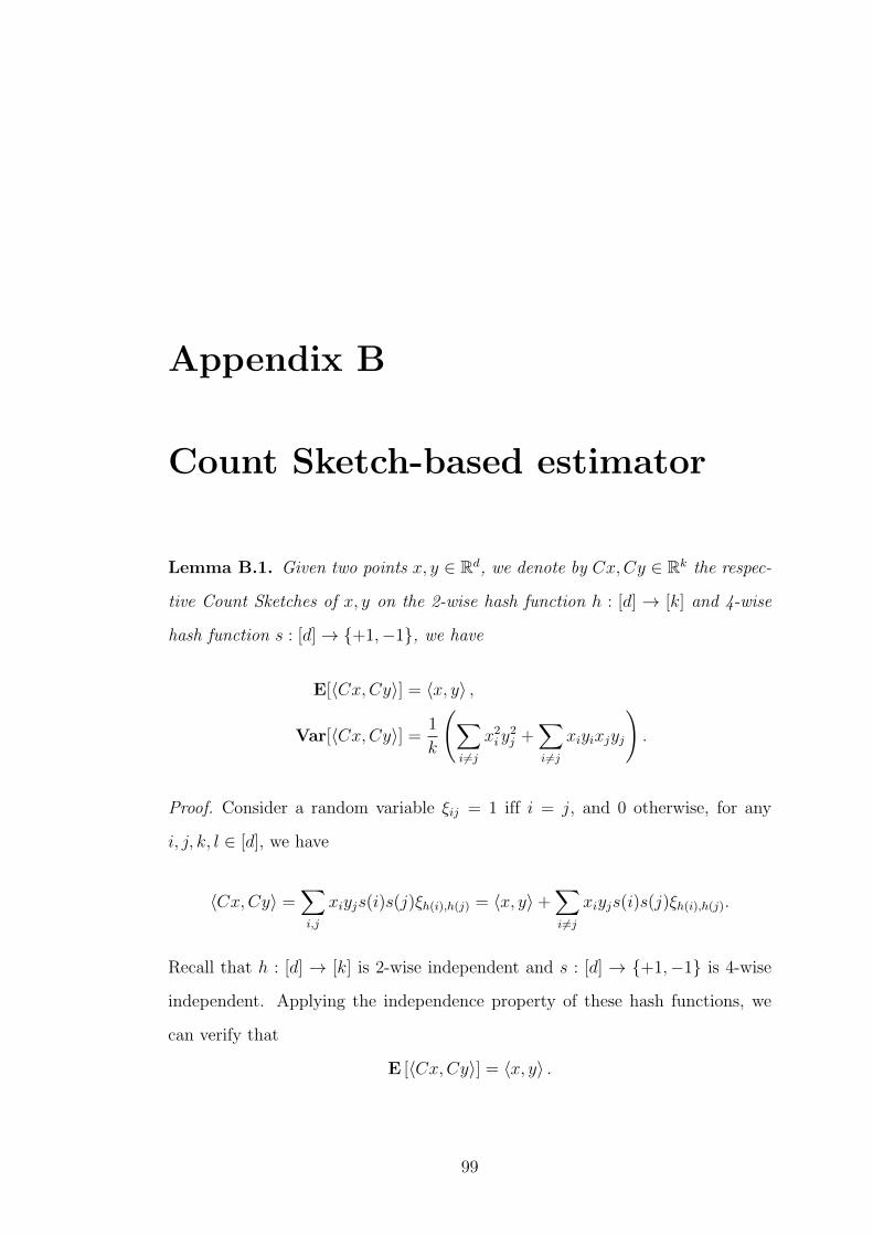
Appendix B

Count Sketch-based estimator

Lemma B.1. Given two points x, y ∈ Rd, we denote by Cx,Cy ∈ Rk the respec-

tive Count Sketches of x, y on the 2-wise hash function h : [d] → [k] and 4-wise

hash function s : [d]→ +1,−1, we have

E[〈Cx,Cy〉] = 〈x, y〉 ,

Var[〈Cx,Cy〉] =1

k

(∑i 6=j

x2i y

2j +

∑i 6=j

xiyixjyj

).

Proof. Consider a random variable ξij = 1 iff i = j, and 0 otherwise, for any

i, j, k, l ∈ [d], we have

〈Cx,Cy〉 =∑i,j

xiyjs(i)s(j)ξh(i),h(j) = 〈x, y〉+∑i 6=j

xiyjs(i)s(j)ξh(i),h(j).

Recall that h : [d] → [k] is 2-wise independent and s : [d] → +1,−1 is 4-wise

independent. Applying the independence property of these hash functions, we

can verify that

E [〈Cx,Cy〉] = 〈x, y〉 .

99

B. COUNT SKETCH-BASED ESTIMATOR

For the variance, we compute E[〈Cx,Cy〉2

]by expanding 〈Cx,Cy〉2 as follows:

〈Cx,Cy〉2 =

(〈x, y〉+

∑i 6=j

xiyjs(i)s(j)ξh(i),h(j)

)(〈x, y〉+

∑k 6=l

xkyls(k)s(l)ξh(k),h(l)

)

= 〈x, y〉2 + 〈x, y〉

(∑i 6=j

xiyjs(i)s(j)ξh(i),h(j) +∑k 6=l


)

+

(∑i 6=j

xiyjs(i)s(j)ξh(i),h(j)

)(∑k 6=l


)

= 〈x, y〉2 + 〈x, y〉

(∑i 6=j

xiyjs(i)s(j)ξh(i),h(j) +∑k 6=l


)

+∑i 6=j,k 6=li=k,j=l

x2i y

2j ξ

2h(i),h(j) +

∑i6=j,k 6=li=l,j=k

xixjyiyjξ2h(i),h(j)

+∑i 6=j,k 6=li=k,j 6=l

x2i yjyls(j)s(l)ξh(i),h(j)ξh(i),h(l) +

∑i 6=j,k 6=li=l,j 6=k

xixkyiyjs(j)s(k)ξh(i),h(j)ξh(k),h(i)

+∑i 6=j,k 6=li 6=k,j=l

xixky2j s(i)s(k)ξh(i),h(j)ξh(k),h(j) +

∑i 6=j,k 6=li 6=l,j=k

xixjyjyls(i)s(l)ξh(i),h(j)ξh(j),h(l)

+∑

i 6=j 6=k 6=l

xiyjxkyls(i)s(j)s(k)s(l)ξh(i),h(j)ξh(k),h(l).

Applying the independence property of hash functions again, we get

E[〈Cx,Cy〉2] = 〈x, y〉2 +1

k

(∑i 6=j

x2i y

2j +

∑i 6=j

xiyixjyj

).

Using the fact that Var[X] = E[X2]− E[X]2 proves the claim of variance.

100

Bibliography

[1] D. Achlioptas. Database-friendly random projections. In Proceedings of

PODS’01, pages 274–281, 2001.

[2] C. C. Aggarwal and P. S. Yu. Outlier detection for high dimensional data.

In Proceedings of SIGMOD’01, pages 37–46, 2001.

[3] N. Ailon and B. Chazelle. Approximate nearest neighbors and the fast

johnson-lindenstrauss transform. In Proceedings of STOC’06, pages 557–

563, 2006.

[4] N. Alon, Y. Matias, and M. Szegedy. The space complexity of approximating

the frequency moments. In Proceedings of STOC’96, pages 20–29, 1996.

[5] Y. Bachrach, E. Porat, and J. S. Rosenschein. Sketching techniques for

collaborative filtering. In Proceedings of IJCAI’09, pages 2016–2021, 2009.

[6] Z. Bar-Yossef, T. Jayram, R. Kumar, D. Sivakumar, and L. Trevisan. Count-

ing distinct elements in a data stream. In RANDOM, pages 1–10. Springer,

2002.

[7] S. D. Bay and M. Schwabacher. Mining distance-based outliers in near lin-

ear time with randomization and a simple pruning rule. In Proceedings of

KDD’03, pages 29–38, 2003.

[8] M. Bendersky and W. B. Croft. Finding text reuse on the web. In Proceedings

of WSDM’09, pages 262–271, 2009.

101

BIBLIOGRAPHY

[9] K. S. Beyer, J. Goldstein, R. Ramakrishnan, and U. Shaft. When is “nearest

neighbor” meaningful? In Proceedings of ICDT’99, pages 217–235, 1999.

[10] V. Braverman, K.-M. Chung, Z. Liu, M. Mitzenmacher, and R. Ostrovsky.

AMS without 4-wise independence on product domains. In Proceedings of

STACS’10, pages 119–130, 2008.

[11] M. M. Breunig, H.-P. Kriegel, R. T. Ng, and J. Sander. LOF: Identifying

density-based local outliers. In Proceedings of SIGMOD’00, pages 93–104,

2000.

[12] A. Z. Broder. On the resemblance and containment of documents. Se-

quences’97, pages 21–29, 1997.

[13] A. Z. Broder, M. Charikar, A. M. Frieze, and M. Mitzenmacher. Min-wise

independent permutations (extended abstract). In Proceedings of STOC’98,

pages 327–336, 1998.

[14] A. Z. Broder, S. C. Glassman, M. S. Manasse, and G. Zweig. Syntactic

clustering of the web. Computer Networks, 29(8-13):1157–1166, 1997.

[15] C.-C. Chang and C.-J. Lin. LIBSVM: A library for support vector ma-

chines. ACM Transactions on Intelligent Systems and Technology, 2:27:1–

27:27, 2011.

[16] M. Charikar. Similarity estimation techniques from rounding algorithms. In

Proceedings of STOC’02, pages 380–388, 2002.

[17] M. Charikar, K. Chen, and M. Farach-Colton. Finding frequent items in

data streams. In Proceedings of ICALP’02, pages 693–703, 2002.

[18] F. Chierichetti, R. Kumar, S. Lattanzi, M. Mitzenmacher, A. Panconesi, and

P. Raghavan. On compressing social networks. In Proceedings of KDD’09,

pages 219–228, 2009.

[19] R. Chitta, R. Jin, T. C. Havens, and A. K. Jain. Approximate kernel k-

means: solution to large scale kernel clustering. In Proceedings of KDD’11,

pages 895–903, 2011.

102

BIBLIOGRAPHY

[20] R. Chitta, R. Jin, and A. K. Jain. Efficient kernel clustering using random

fourier features. In Proceedings of ICDM’12, pages 161–170, 2012.

[21] E. Cohen, M. Datar, S. Fujiwara, A. Gionis, P. Indyk, R. Motwani, J. D. Ull-

man, and C. Yang. Finding interesting associations without support pruning.

IEEE Trans. Knowl. Data Eng., 13(1):64–78, 2001.

[22] A. Das, M. Datar, A. Garg, and S. Rajaram. Google news personalization:

scalable online collaborative filtering. In Proceedings of WWW’07, pages

271–280, 2007.

[23] S. Dasgupta and A. Gupta. An elementary proof of the Johnson-

Lindenstrauss lemma. Technical report, International Computer Science

Institute, Berkeley, US, 1999.

[24] J. Dean and S. Ghemawat. MapReduce: Simplified data processing on large

clusters. In Proceedings of OSDI’04, pages 137–150, 2004.

[25] P. Drineas and M. W. Mahoney. On the Nystrom method for approximat-

ing a gram matrix for improved kernel-based learning. Journal of Machine

Learning Research, 6:2153–2175, 2005.

[26] D. Eppstein, M. T. Goodrich, F. Uyeda, and G. Varghese. What’s the

difference?: efficient set reconciliation without prior context. In Proceedings

of SIGCOMM’11, pages 218–229, 2011.

[27] R.-E. Fan, K.-W. Chang, C.-J. Hsieh, X.-R. Wang, and C.-J. Lin. LIBLIN-

EAR: A library for large linear classification. Journal of Machine Learning

Research, 9:1871–1874, 2008.

[28] S. Fine and K. Scheinberg. Efficient SVM training using low-rank kernel

representations. Journal of Machine Learning Research, 2:243–264, 2001.

[29] A. Frank and A. Asuncion. UCI machine learning repository, 2010.

[30] A. Ghoting, S. Parthasarathy, and M. E. Otey. Fast mining of distance-

based outliers in high-dimensional datasets. Data Mining and Knowledge

Discovery, 16(3):349–364, 2008.

103

BIBLIOGRAPHY

[31] M. X. Goemans and D. P. Williamson. Improved approximation algorithms

for maximum cut and satisfiability problems using semidefinite program-

ming. Journal of the ACM, 42(6):1115–1145, 1995.

[32] S. Gollapudi and R. Panigrahy. Exploiting asymmetry in hierarchical topic

extraction. In Proceedings of CIKM’06, pages 475–482, 2006.

[33] S. Gollapudi and A. Sharma. An axiomatic approach for result diversifica-

tion. In Proceedings of WWW’09, pages 381–390, 2009.

[34] M. R. Henzinger. Finding near-duplicate web pages: a large-scale evaluation

of algorithms. In Proceedings of SIGIR’06, pages 284–291, 2006.

[35] A. Hinneburg, C. C. Aggarwal, and D. A. Keim. What is the nearest neighbor

in high dimensional spaces? In Proceedings of VLDB’00, pages 506–515,

2000.

[36] P. Indyk and A. McGregor. Declaring independence via the sketching of

sketches. In Proceedings of SODA’08, pages 737–745, 2008.

[37] P. Indyk and R. Motwani. Approximate nearest neighbors: Towards remov-

ing the curse of dimensionality. In Proceedings of STOC’98, pages 604–613,

1998.

[38] S. Ioffe. Improved consistent sampling, weighted minhash and l1 sketching.

In Proceedings of ICDM’10, pages 246–255, 2010.

[39] T. Joachims. Training linear SVMs in linear time. In Proceedings of KDD’06,

pages 217–226, 2006.

[40] W. B. Johnson and J. Lindenstrauss. Extensions of Lipschitz mappings into

a Hilbert space. Contemporary mathematics, 26(189-206):1, 1984.

[41] P. Kar and H. Karnick. Random feature maps for dot product kernels. In

Proceedings of AISTATS’12, pages 583–591, 2012.

[42] E. M. Knorr and R. T. Ng. Algorithms for mining distance-based outliers in

large datasets. In Proceedings of VLDB’98, pages 392–403, 1998.

104

BIBLIOGRAPHY

[43] H.-P. Kriegel, M. Schubert, and A. Zimek. Angle-based outlier detection in

high-dimensional data. In Proceedings of KDD’08, pages 444–452, 2008.

[44] H.-P. Kriegel, M. Schubert, and A. Zimek. Outlier detection techniques. In

Tutorial at KDD’10, 2010.

[45] K. Kutzkov, A. Bifet, F. Bonchi, and A. Gionis. STRIP: stream learning of

influence probabilities. In Proceedings of KDD’13, pages 275–283, 2013.

[46] Q. V. Le, T. Sarlós, and A. J. Smola. Fastfood - computing hilbert space

expansions in loglinear time. In Proceedings of ICML’13, pages 244–252,

2013.

[47] Y. LeCun, L. Bottou, Y. Bengio, and P. Haffner. Gradient-based learning

applied to document recognition. Proceedings of the IEEE, 86:2278–2324,

1998.

[48] P. Li and A. C. Konig. b-bit minwise hashing. In Proceedings of WWW’10,

pages 671–680, 2010.

[49] P. Li, A. Shrivastava, J. L. Moore, and A. C. Konig. Hashing algorithms for

large-scale learning. In Advances in NIPS’11, pages 2672–2680, 2011.

[50] V. Mahadevan, W. Li, V. Bhalodia, and N. Vasconcelos. Anomaly detection

in crowded scenes. In Proceedings of CVPR’10, pages 1975–1981, 2010.

[51] S. Maji and A. C. Berg. Max-margin additive classifiers for detection. In

Proceedings of ICCV’09, pages 40–47, 2009.

[52] M. Manasse, F. McSherry, and K. Talwar. Consistent weighted sampling.

MSR-TR-2010-73 technical report, 2010.

[53] G. S. Manku, A. Jain, and A. D. Sarma. Detecting near-duplicates for web

crawling. In Proceedings of WWW’07, pages 141–150, 2007.

[54] M. Mitzenmacher and E. Upfal. Probability and Computing: Randomized

Algorithms and Probabilistic Analysis. Cambridge University Press, 2005.

105

BIBLIOGRAPHY

[55] E. Muller, M. Schiffer, and T. Seidl. Statistical selection of relevant subspace

projections for outlier ranking. In Proceedings of ICDE’11, pages 434–445,

2011.

[56] E. Osuna, R. Freund, and F. Girosi. An improved training algorithm for

support vector machines. In Proceedings of NNSP’97, pages 276–285, 1997.

[57] R. Pagh. Compressed matrix multiplication. In Proceedings of ICTS’12,

pages 442–451, 2012.

[58] S. Papadimitriou, H. Kitagawa, P. B. Gibbons, and C. Faloutsos. LOCI:

Fast outlier detection using the local correlation integral. In Proceedings of

ICDE’03, pages 315–326, 2003.

[59] M. Patrascu and M. Thorup. The power of simple tabulation hashing. In

Proceedings of STOC’11, pages 1–10, 2011.

[60] A. Rahimi and B. Recht. Random features for large-scale kernel machines.

In Advances in NIPS’07, pages 1177–1184, 2007.

[61] S. Ramaswamy, R. Rastogi, and K. Shim. Efficient algorithms for mining

outliers from large data sets. In Proceedings of SIGMOD’00, pages 427–438,

2000.

[62] B. Schokopf and A. J. Smola. Learning with kernels: Support vector ma-

chines, regularization, Optimization, and Beyond. MIT Press, 2001.

[63] E. F. Schuster and A. N. Philippou. The odds in some odd-even games. The

American Mathematical Monthly, 82:646–648, 1975.

[64] S. Shalev-Shwartz, Y. Singer, and N. Srebro. Pegasos: Primal estimated

sub-gradient solver for SVM. In Proceedings of ICML’07, pages 807–814,

2007.

[65] A. J. Smola and B. Schokopf. Sparse greedy matrix approximation for ma-

chine learning. In Proceedings of ICML’00, pages 911–918, 2000.

106

BIBLIOGRAPHY

[66] M. Thorup and Y. Zhang. Tabulation-based 5-independent hashing with

applications to linear probing and second moment estimation. SIAM J.

Comput., 41(2):293–331, 2012.

[67] T. Urvoy, E. Chauveau, P. Filoche, and T. Lavergne. Tracking web spam

with html style similarities. TWEB, 2(1), 2008.

[68] A. Vedaldi and A. Zisserman. Efficient additive kernels via explicit feature

maps. In Proceedings of CVPR’10, pages 3539–3546, 2010.

[69] S. S. Vempala. The Random Projection Method. American Mathematical

Society, 2003.

[70] S. Vempati, A. Vedaldi, A. Zisserman, and C. V. Jawahar. Generalized RBF

feature maps for efficient detection. In Proceedings of BMVC’10, pages 1–11,

2010.

[71] Y. Wang, S. Parthasarathy, and S. Tatikonda. Locality sensitive outlier

detection: A ranking driven approach. In Proceedings of ICDE’11, pages

410–421, 2011.

[72] M. N. Wegman and L. Carter. New hash functions and their use in au-

thentication and set equality. Journal of Computer and System Sciences,

22(3):265–279, 1981.

[73] K. Q. Weinberger, A. Dasgupta, J. Langford, A. J. Smola, and J. Atten-

berg. Feature hashing for large scale multitask learning. In Proceedings of

ICML’09, pages 1113–1120, 2009.

[74] R. Wheeler and J. S. Aitken. Multiple algorithms for fraud detection. Knowl-

edge Based Systems, 13(2-3):93–99, 2000.

[75] C. K. I. Williams and M. Seeger. Using the Nystrom method to speed up

kernel machines. In Advances in NIPS’01, pages 682–688, 2001.

[76] T. Yang, Y.-F. Li, M. Mahdavi, R. Jin, and Z.-H. Zhou. Nystrom method

vs random fourier features: A theoretical and empirical comparison. In

Advances in NIPS’12, pages 485–493, 2012.

107

Documents

On the Power of Randomization in Big Data Analytics including nearest neighbor search, outlier detection and classifica-tion. Theseconceptsarealsobasicdataanalysisproblemsthatthethesisaims