On the Numerical Radius and Its Applications* · Department of Applied Mathematics California Institute of Technology Pasadena, California 91125 Submitted by M. Newman ABSTRACT We

On the Numerical Radius and Its Applications*

Moshe Goldberg’

Department of Mathematics Technion-Israel Institute of Technology Haifa, Israel and Znstitute for the interdisciplinary Applications of Algebra and Combinatorics University of Califmia Santa Barbara, Califmia 93106

and

Eitan Tadmor

Department of Applied Mathematics California Institute of Technology Pasadena, California 91125

Submitted by M. Newman

ABSTRACT

We give a brief account of the numerical radius of a linear bounded operator on a Hilbert space and some of its better-known properties. Both finite- and infinite- dimensional aspects are discussed, as well as applications to stability theory of finite-difference approximations for hyperbolic initial-value problems.

1. DEFINITION, BOUNDS, AND EVALUATION

Let H be a Hilbert space over the complex field C with inner product

(x,y) and norm llxll=(x,x) ‘/’ Let C&(H) denote the algebra of bounded linear . operators on H. Then, for any A in %3(H) we define the numerical radius of

*Notes solicited by Professor Morris Newman, following a series of lectures delivered by the first author at the Institute for the Interdisciplinary Applications of Algebra and Combinatorics,

University of California, Santa Barbara, California, Summer 1980. ‘Research sponsored in part by the Air Force Office of Scientific Research, Air Force System

Command, United States Air Force Grant Nos. AFSOR-763046 and AFSOR-799127.

LINEAR ALGEBRA ANDITSAPPLZCATZONS42:263-284 (1982) 263

0 Elsevier Science Publishing Co., Inc., 1982

52 Vanderbilt Ave., New York, NY 10017 0024-3795/82/010263 + 22$02.75

264

A.

MOSHE GOLDBERG AND EITAN TADMOR

r(A)=sup{~(Ar,r)~:~~~~~=l}.

Three of the most obvious properties of r are:

r(A)>@

r(oA)=]a]r(A) V’aEC;

r(A+B)+A)+r(B) VA, BE%(H).

(1.1)

(1.2)

(1.3)

In this section we discuss further bounds for r as well as ways to evaluate it.

THEOREM 1.1 (e.g. [ll], [18]). Let p(A) be the spectral radiu.s ofA. Then

p(A) -(A). (1.4)

Proof. Denoting the spectrum of A by A( A) and its numerical range by

W(A)= {(Ax,x):Ilxll=l},

we shall show that

Since

A(A)c W(A).

r(A)=sup{]z]:zEW(A)}, (1.5)

this will imply the desired result. In the finite-dimensional case the proof is simple: if A is an eigenvalue of A

with a corresponding unit eigenvector x, then

so

ON THE NUMERICAL RADIUS

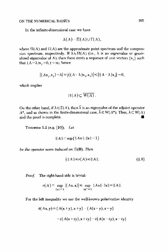
In the infinite-dimensional case we have

A(A)=II(A)UI’(A),

265

where II(A) and lY( A) are the approximate point spectrum and the compres- sion spectrum, respectively. If X EII(A) (i.e., A is an eigenvalue or gener- alized eigenvalue of A), then there exists a sequence of unit vectors {xi} such that (A--A)xi-+O, j-cc; hence

which implies

WA& W(A).

On the other hand, if h E I( A), then x is an eigenvalue of the adjoint operator A*, and as shown in the finite-dimensional case, i E W( A*). Thus, X E W(A)

and the proof is complete. n

THEOREM 1.2 (e.g. [lo]). Let

II A II =sup{ II Ad: llxll= l}

be the operator rwrm induced on 3(H). Then

Proof. The right-hand side is trivial:

r(A) = ,,yl Ikkx)I s sup II Axll . Ml = II A II. x IIXII = 1

For the left inequality we use the well-known polarization identity

4(Ax,y) = (A(x+y),x+y) - (A+y),x-y)

(1.6)

+i(A(x+iy),x+iy) -i(A(x-iy),x-iy)

266 MOSHE GOLDBERG AND EITAN TADMOR

and the parallelogram law

which are easily obtained by expanding their right- and left-hand sides, respectively. We find that

hence

~u~{~(Ax,y)~:Ilxll=llyll=1}~2r(A). (1.7)

In particular, if y is a unit vector in the direction of Ax, then 1 (Ax,y)] = 1) AxI], and substituting in (1.7) the theorem follows. n

By (1.4) and (1.6) we have

p(A)+4)~IIAIl VA E%(H). (1.8)

Since if A is normal then p(A)= I] A ]I (e.g. [ZO]), we conclude that

~(A)=r(A)=llAll forrwrmulA. 0.9)

Following Halmos [ 111, we say that A is spectral if

By (1.9), therefore, normal operators are spectral. The converse, however, is false, as shown in Example 2.1 below; the class of normal operators is a proper subclass of the spectral ones.

Characterizations of spectral operators were given by Furuta and Takeda [4]; Goldberg, Tadmor, and Zwas [8]; and Goldberg [5]. Wintner [22] (see also [ll]) has shown that operators satisfying r(A)= ]I A ]I are spectral as well.

Having (1.9), we should perhaps mention a shorter proof of the left-hand side of (1.6): We write A as a sum of normal operators,

A=;(A+A*)+i(A-A*),

ON THE NUMERICAL RADIUS 267

and observe that

r(A)=r(A*);

so by (1.3)

IIAII+IIA+A*ll+$lA-A*II=$r(A+A*)+&r(A-A*)

which gives the desired result. Two additional results, often useful in evaluating r(A), are given in the

following theorem.

THEOREM 1.3.

(i) The numerical radius is invariant under unitary similurities, i.e., for any unitary operator U,

r(U*AU)=r(A). (1.10)

(ii) ZfH=H,@H, is a direct sum and A, E%(H,), As ~?h(Hs), then

r(A1~A2)=max{r(A,),r(A2)}. (1.11)

Proof. For (i) we have

For (ii), we write A=A,@A, and let W(A,), j= 1,2, be the numerical range of Aj. Evidently, W(A,) c W(A); thus

(conv for convex huh). (1.12)

Conversely, for any unit vector x we write x=xl+xz, where x,EH,, x,EH,, and llxr II2 + llxe II2 = l/x/l 2 = 1. Setting unit vectors yr =xl/JIxl )I E


H,, y2 =x2/llx2 II EH2, we have

so

W(A)=conv{ W(A,),W(A,)}. (1.13)

By (1.12), (1.13), therefore,

and (1.5) implies (1.11). n

2. THE FINITE-DIMENSIONAL CASE

We come now to discuss concrete computations of r(A) in the finite- dimensional case where we may of course restrict attention to H=C”, the space of complex n-tuples with some inner product, and to %(H)=C,,,, the algebra of complex nXn matrices.

Indeed, let (x,y) be an inner product on C”; let e,, . . . ,e, be the standard basis of C”; and set pii =(ei,ei), l~i, 1 ‘< n. Then the matrix P =( pii) is Hermitian, and for any two vectors

x= X1’...,X”)” ( y=(Y1,...,Yn)‘EC”

(prime denoting the transpose), we have

Since (x,x)>0 for x#O, we obtain the known result that (x, y) is an inner product on C” if and only if it is of the form

(x,y) = (x,y)p=y*px (2.1)

So we see that in the finite-dimensional case it suffices to study numerical radius

269 ON THE NUMERICAL RADIUS

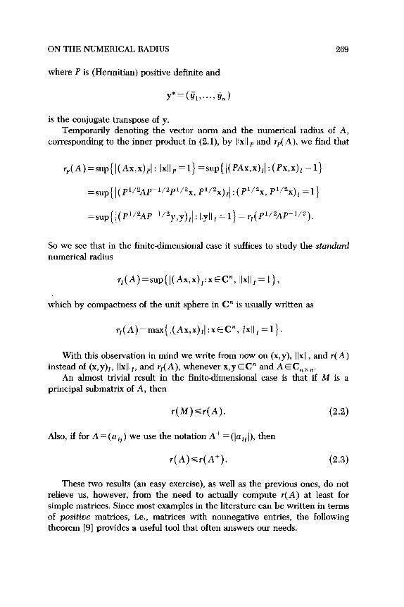
where P is (Hermitian) positive definite and

y*=(&...&)

is the conjugate transpose of y. Temporarily denoting the vector norm and the numerical radius of A,

corresponding to the inner product in (2.1), by llxll p and rp(A), we find that

r,(A)=sup{~(Ax,x),~:llxll~=1}=sup{~(~Ax,x),~:(Px,x)~=1}

=sup{ I(P’/‘AP- l/2Pl/2x, P1/2x)II : (P”2X, P”2x)I = l}

=s~p{~(P~~~AP-~~~y,y),~:~~y~l~=l}=r~(P~’~AP-~’~’

the standard

T~(A)=suP{I(Ax,x)~:xEC”, IlxllI=l},

which by compactness of the unit sphere in C” is usually written as

With this observation in mind we write from now on (x,y), Ilxll, and r(A) instead of (~,y)~, llxll I9 and r,(A), whenever x,y~C” and AEC,,,.

An almost trivial result in the finite-dimensional case is that if M is a principal submatrix of A, then

r(M)+A).

Also, if for A=(aii) we use the notation A+=(laiil), then

(2.2)

r(A)<r(A+). (2.3)

These two results (an easy exercise), as well as the previous ones, do not relieve us, however, from the need to actually compute r(A) at least for simple matrices. Since most examples in the literature can be written in terms of positive matrices, i.e., matrices with nonnegative entries, the following theorem [9] provides a useful tool that often answers our needs.


THEOREM 2.1.

(i) Let A be a positive matrix. Then

r(A)=p(ReA) [ReA=&(A+A’)].

(ii) Consider the real symmetric matrix

If

S(a)=al-ReA, UER.

D=diag(ar,...,a.)

is a diagonal matrix congruent to S(a), then r(A) = u if and only if the a i are nonnegative and at least one of them does not vanish.

Proof Since

r(A)=max{l(Ax,x)l:xEC”, (x,x)=1},

then there exists a unit vector x0 = (x1, . . . , x, )’ E C” such that r(A)=I(Ax,,x,)]. Since A is a positive matrix and y=(Ixll,...,Ixnl)’ is a positive unit vector, it follows that

so

r(A)=max{(Ax,x):xERn, (x,x)=1}.

Similarly, since Re A is positive, then

r(ReA)=max{(ReAx,x):xER”, (x,x)=1}.

Now, since it is not hard to see that (ReAx,x) = (Ax,x) for all x ER”, then r(A)= r(ReA), and (1.9) implies (i).

For part (ii) we mention again that

r(A)=max{(ReAx,x):xER”,(x,x)=l}.


Hence, r(A)= (I for some (I >O, if and only if (ReAx,x)G a(x,x) for all xER” with equality for some x,ER”. That is, r(A)= u only if the real symmetric matrix S(u) = OZ - Re A is positive semidefinite but not positive definite, or in other words, if the eigenvalues of S(u) are nonnegative and at least one of them vanishes. Thus, part (ii) is now an immediate consequence of Sylvester’s law of inertia, and the proof is complete. n

EXAMPLE 2.1. Often in examples we encounter 2 X 2 positive matrices of

the form

A=( :’ i2) [or A=( 1’ ~a)].

By Theorem 2.1(i), therefore,

(2.4a)

r(A)=p(ReA)=j(a,+a,)+~J(a,-a,)2+b2. (2.4b)

This result also follows from the known fact that if a,, u2, and b in (2.4a) are any complex numbers, then the numerical range, W(A), is the (possibly degenerate) elliptic disc &(a,, u2, lbl) with foci at a,, a2 and minor axis Ibl. As Halmos puts it, however, the proof of this assertion (e.g. Mumaghan [15], Donoghue [3]) is analytic geometry at its worst; hence our direct computation of r(A) in (2.4b) is indeed much shorter.

We can now easily answer a question raised in Section 1: Using (1.11) and (2.4), we find that the nXn nonnormal matrix

satisfies r(A)=p( A)= 1, showing how far from normal a spectral operator can be.

We note that since any matrix is unitarily similar to a triangular matrix and since both the numerical radius and the spectrum are invariant under unitary similarities, then it is easy to see that a 2X2 matrix is spectral if and only if it is normal.

EXAMPLE 2.2. Consider the nilpotent matrix

0 100’ 0 0 101


and let us compute r(A*), m= 1,2,3. Starting with the easiest case, we interchange the first and third rows and columns of A3 to find that A3 is unitarily similar to the matrix

hence by (1.11) and (2.4),

r(A3)=+.

Similarly, interchanging the second and third rows and columns of A2, we obtain

r(A2)=&.

To find r(A), we may employ Theorem 2.1(i) to verify that

r(A)=p(ReA)=(1+$)/4.

This value of r(A) may be conveniently obtained by alternately operating on the columns and rows of the matrix S = aZ- Re A with elementary operations, to eliminate its off-diagonal entries s~,~, s2,r, s~,~, s~,~, s~,~, s~,~ (in that order) and to find that S is congruent to

D=diag(a,,a,,a,,a,)

with

or=u, q=(J--‘a71 4 1-l’ j=2,3,4.

Hence a,~u,>,u,~u,=0 if and only if 0=(1+6)/4, and Theorem 2.l(ii) yields the above result.

3. SOME NORM PROPERTIES

As usual, we calf a mapping A +IV( A) a semirwrm on %3(H) if for alI A, BE%(H) and CXEC,

N(A)aO, (3.la)

N(aA)=l+‘(A), (3.lb)

N(A+B)GV(A)+N(B). (3.lc)


If in addition N satisfies

N(A)>0 for AZO, (3.ld)

then N is a norm on a(H), which may or may not be related to the given operator norm.

Having the above definitions, the relations (l.l)-(1.3) imply that r is a seminorm on %3(H). In fact we can easily show more:

THEOREM 3.1. The numerical radius is a rwrm on a(H).

Proof. We have to check (3.ld), or alternatively to show that r(A)=0 implies A=O. But then, by (1.6), IIAIIG2r(A)=O; so IIAIl=O and our claim follows. n

Theorems 1.2 and 3.1 indicate that r and the operator norm on 93(H) are certainly related. There is, however, one important feature, namely (sub-) multiplicativity, which separates the two. More precisely, while

II AB II d II A II . II B II VA, BE%(H),

the inequality

r(AB)Gr(A)r(B) (3.2)

is disappointingly false. To demonstrate this, take the matrices,

By (2.4), r( A)=r( B)= i, r( AB)= 1, and so much for multiplicativity. In fact, Brown and Shields [ 161 have considered the 4 X 4 matrix in Example 2.2, for which

So in general (2.2) may fail even when A and B commute, or worse yet, when A and B are powers of the same operator.


What is true with respect to multiplicativity, however, is the following remarkable result, conjectured by Halmos and first proved by Berger [l].

THEOREM 3.2. For any A E’@H),

r(Am)W’(A), m=1,2,3,...; (3.3)

OT equivalently,

r(A)<1 implies r(A”)~l, m=1,2,3 ,... . (3.4)

Proof Clearly, (3.3) implies (3.4). Conversely, suppose (3.4) holds. If A = 0 then there is nothing to prove, so assume A #O, and consider the operator B=A/r(A). By (1.2), r(B)= 1; hence, r(P)6 1. It follows that r(A’“/r”‘(A))< 1, and by (1.2) again, we obtain (3.3). Consequently, (3.3) and (3.4) are equivalent and it suffices to prove (3.4).

For this purpose let m be a positive integer; let

oi =pii/m, i=l,...,m,

be the mth roots of unity, and consider the polynomial identities

(3.5)

which obviously hold when z is replaced by any operator B E%(H). Now, for an arbitrary unit vector x E H define the vectors

j=l,...,m,


and use (3.5), (3.6) to find that

In particular, setting

(3.7) yields

B=Ae”, 9ER,

(3.7)

-$1\1xi112[l-~,eie( $,&)]=l-eime(A”‘x,x). I

Since by hypothesis r(A) G 1, the real part of the expression in the brackets above is nonnegative. So for any unit vector x and real 8,

Re[ 1 -eime( A”‘x,x)] 20;

thus

j(Amx,x)l~l, llxll = 1,

and (3.4) follows.


The above proof is due to Pearcy [16]. We note that the rather interesting evolution of Berger’s theorem is described in [2] and [5].

It might be useful to remark that by (1.6) and (3.3),

so we have

COROLLARY 3.1. Zf r( A)< 1, then the operator rwrm on C%(H) satisfies

II A”’ II s2, m=1,2,3 ,... .

Although the numerical radius is nonmultiplicative, a simple multiplica- tion by a scalar may correct this situation, as shown in our next result [6].

THEOREM 3.3. Let v>O befixed, and consider thefunction r,(A)- VT(A). Then:

(i) r, is a rwrm on ‘%3(H). (ii) r, is multiplicative on %3(H) if and only if ~24.

Proof. The statement in (i) is trivial and holds for NV -vN, N being any norm on a(H).

To prove (ii), fix some ~24. Then for ail A, BE’%(H), (1.6) implies

i.e., r, is multiplicative. Conversely, to show that v = 4 is the least factor for which r, is multiplica-

tive, consider the matrices

A=(; ;), Z3=(‘: 8).

By (2.4), r(A)= r(B)=+, r(AB)= 1. Hence for these matrices r, satisfies

if and only if ~24, and the theorem follows.


It is worth noting that if N is an arbitrary norm on a finite-dimensional algebra, then multiplicativity factors, i.e. constants v>O for which NV G vN is multiplicative, always exist [6]. This, however, is not always true in the infinite-dimensional case [7].

4. APPLICATIONS: STABLE LAX-WENDROFF SCHEMES

Consider the first-order, linear, 2space-dimensional hyperbolic system of partial differential equations

u, =Au, +Bu,, -WcO(x~W, -wocycw, t20, (4.la)

where u=(u,(x, y, t) ,..., u,(x, y, t))’ is an unknown vector; A and B fixed n X n Hermitian coefficient matrices; and u x, u y, and u t the partial deriva- tives of u with respect to the independent variables x, y, and t. It is well known (e.g. [17]) that the solution of (4.la) is uniquely determined and well posed in L2( - co, co), if proper initial values

u(x, y,o) =f(x, y) EL2( - 00, co), -cooo(x~Qo, -cocy<w,

(4.lb)

are prescribed. In order to solve (4.1) by finite-difference approximations we introduce

increments Ax>O, Ay>O, At>0 with fixed ratios X=At/Ax, p=At/Ay; grid points

(xi,yk,tm)=(iAx,kAy,mAt), i,k=O,*l,-t2 ,..., m=0,1,2 ,...;

and the notation

Then a Taylor expansion of a sufficiently smooth solution of (4.la) about (xi, y,, t,) can be written as

u;+l =u; +At(u,);+i(At)2(u,,);+O(At3). (4.2)

278

Since by (1.4a),

MOSHE GOLDBERG AND EITAN TADMOR

utt = (Au,+Bu,)~=Au,,+Bu,,

=A(Au, +Bu,)~+B(Au, +Bu~)~=A~u,, +B2u,, +(AB+BA)u.,,

then (4.2) yields

so using the standard difference formulas

+O(Ax)+O(Ay)+O(Ax2,‘Ay)+O(Ay2/Ax)

and the relations

Ax=A At, Ay=p At (h, p constants),

we find that

u~+‘=u~+&XA(u~+l,k-~~-l,k)+~~B(~~k+l-~;fk_l)

+ ~h2A2(~7+l,k-2~;+~7--l,k) + ;~L~B~(u~~+,-~u;+u~~_~)

+~h~(AB+~A)(u~+‘,,,k+l-u;1+1,k--l-u~-l,k+l+u~---1,k--l)+O(At3)


Thus, dropping 0(At3) terms and replacing u by an approximation vector v, we finally obtain the celebrated Lax-Wendroff difference scheme for (l.l), [13]:

(4.3a)

which may be solved, time step after time step, if initial values

v$=f+ff(rj,&), j,k=O,*1,*2 ,..., (4.3b)

are set. The main question concerning the scheme (4.3) is whether it is conoer-

gent; that is, keeping the ratios h and p fixed and letting At-O, we ask if the numerical solution v of (4.3) tends to that of (4.1).

In order to answer this question we introduce the amplification matrix

+QAp(AB+BA)(e i(E+?) -ei(~-~) -ei(S-E) +e-i(E+~)), (4.4)

which is the Fourier transform of the difference operator associated with our scheme, formally obtained by taking the right-hand side of (4.3a) with vi”+,, k+q replaced by the Fourier component ei(Pf+9’r). We say that the scheme (4.3) is stable if G is power bounded, i.e., if for some norm N on CnXn and a fixed constant K>O,

@&~J,P)*]~~ Vm=1,2,3 ,,.., -~<.$<a, --n<q<a.

(4.5)

Traditionally (e.g. [17]) this definition is stated with the spectral norm rather than an arbitrary IV. However, since all norms on C,,, are equivalent, it makes no difference with respect to which norm the estimate in (4.5) is taken, and in particular we may use the numerical radius.


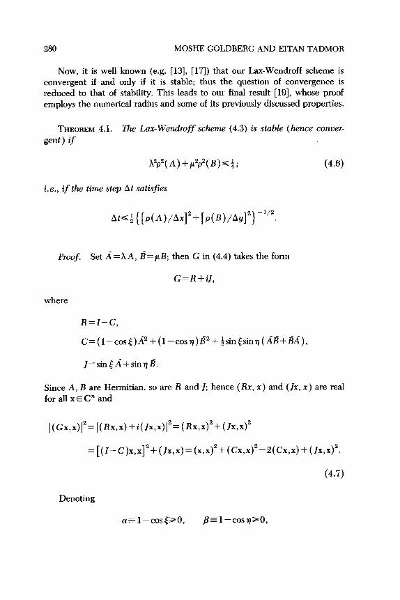
Now, it is well known (e.g. [13], [17]) that our Lax-Wendroff scheme is convergent if and only if it is stable; thus the question of convergence is reduced to that of stability. This leads to our final result [19], whose proof employs the numerical radius and some of its previously discussed properties.

THEOREM 4.1. The Lax-We&off scheme (4.3) is stable (hence conver-

gent) if

&“(A)+p2p2(B)+; (4.6)

i.e., if the time step At satisfies

Proof. Set A=hA, B=pLB; then G in (4.4) takes the form

G=R+iJ,

where

R=Z-C,

C=(l-cost)A2+(1-cosn)B2+~sin[sinq(dB+BA),

J=sin[d+sinrjB.

Since A, B are Hermitian, so are R and J; hence (Rx, x) and (Jr, x) are real for all x EC” and

Denoting


we easily verify that

c=&((u%2+p%2+J2).

Thus,

2(cx,x)=(Y2(d2x,x)+p~(B2x,x)+(J2x,x)

=a2(Ax, Ax)+p2(Bx, Bx)+(Jx, Jx)

+(u211dx112+~211Bxl12+llJXl12. (4.8)

Since also

( lx,x)2s II Jxll 2 Ml 2 = II 1x11 2, llxll = 1, (4.9)

then (4.7)-(4.9) yield

((Gx,x)~~~~+(CX,X)~-~~II~~~~~-~~~~~X~~~, llxll= 1. (4.10)

Next, we write

SO

I(c”,“>I”“((~2x~x)I+PI( B2x,x)~+~~sin~sin~((AB+Bd)x,x)~.

(4.11)

We have

(isin[sinv((AB+BA)x,x)l


Therefore (4.11) gives

~(Cx,x)~~2a!IIAxll~+2~IIBxll~,

and by the Cauchy-Schwarz inequality,

(CX,X)2=~(CX,X)~2~4(c-llAxl12+~IIBxl12)2

~4(a211Axl12+~211Bx112)(lIAxl12+lIBxl12). (4.12)

Since A, I? are Hermitian, then by (1.9),

ll~xll~ll~lIMl=II~Il=p(~)=Xp(A), llxll = 1,

and similarly

IIBxll~pp(B), Ml = 1.

Thus, by (4.12) and the hypothesis (4.6),

(Cx,x)2 ~a2IIAxll2+P2IIBxll2,

and (4.10) implies

](Gx,x)(~<~, I]xl]=l.

Consequently, r(G)< 1; so by Theorem 3.2,

r(G”)<l, m=1,2,3 ,...,

and the proof is complete. n

In their original paper, Lax and Wendroff [13] were the first to utilize numerical-radius techniques for stability purposes, proving that the scheme (4.3) is stable if

(4.13)


Evidently, the condition (4.6)-allowing a larger time step-is an improve- ment over (4.13) unless hp(A)= pp(B), in which case the two conditions coincide.

It is a straightforward matter to follow the construction in (4.2)-(4.5) and obtain a scheme, analogous to (4.3), for the d-dimensional hyperbolic system

d

ut= I: Aju,jt -mooxi~oo, t 20, (4.14) j=l

where as before, the Ai are fixed n X n Hermitian matrices. It is not hard to see that for this multidimensional Lax-Wendroff scheme, the conditions (4.6) and (4.13) become

5 +Z(A,)<$ (Ai=At,‘Axi) i=l

and

(4.15)

(4.16)

respectively. Thus as in the 2dimensional case, the advantage of (4.15) over (4.16) is evident, unless the h,p(A,) are all equal.

In case A and B in (4.6) are real and symmetric, Turkel[21] has improved (4.6), showing that the scheme (4.3) is stable if

which again coincides with (4.6) and (4.13) when Xp(A)= pp(B). It seems, however, that Turkel’s interesting result for (4.3) does not go over to the general &dimensional case.

We remark that Livne [14] and Iusim [12] have used similar techniques to successfully investigate the stability of other difference schemes for hyperbolic systems of type (4.1) and (4.14) with d ~3.

REFERENCES

1 C. A. Berger, On the numerical range of powers of an operator, Abstract No. 625-152, Notices Amer. Math. Sot. 12:5QO (1965).


2 C. A. Berger and J. G. Stampfli, Mapping theorems for the numerican range, Amer. J. Math. 89:1047-1055 (1967).

3 W. F. Donoghue, On the numerical range of a bounded operator, Michigan Math. J. 4:261-263 (1957).

4 T. Furuta and Z. Takeda, A characterization of spectraloid operators and its generalizations, Proc. Japan Acad. 43:599-604 (1967).

5 M. Goldberg, On certain finite dimensional numerical ranges and numerical radii, Linear and Multilinear Algebra 7:329-342 (1979).

6 M. Goldberg and E. G. Straus, Norm properties of C-numerical radii, Linear Algebra Appl. 24:113-131 (1979).

7 M. Goldberg and E. G. Straus, Operator norms, multiplicativity factors, and C-numerical radii, Linear Algebra Appl., to appear.

8 M. Goldberg, E. Tadmor, and G. Zwas, The numerical radius and spectral matrices, Linear and Mu&linear Algebra 2:317-326 (1975).

9 M. Goldberg, E. Tadmor, and G. Zwas, Numerical radius of positive matrices, Linear Algebra Appl. 12:209-214 (1975).

10 P. R. Halmos, introduction to Hilbert Space and the Theory of Spectral Multiplic- ity, Chelsea, New York, 1951.

11 P. R. Halmos, A Hilbert Space Problem Book, Van Nostrand, New York, 1967. 12 R. Iusim, An explicit method for solving three dimensional symmetric hyperbolic

equations, M.Sc. Thesis, Dept. of Math., Technion-Israel Inst. of Technology, 1979.

13 P. D. Lax and B. Wendroff, Difference schemes for hyperbolic equations with high order of accuracy, &mm. Pure Appl. Math. 17:381-391 (1964).

14 A. Livne, Seven point difference schemes for hyperbolic equations, Math. Camp. 29:425-433 (1975).

15 F. D. Murnaghan, On the field of values of a square matrix, Proc. Nut. Acad. Sci. U.S.A. 18:246-248 (1932).

16 C. Pearcy, An elementary proof of the power inequality for the numerical radius, Michigan Math. J. 13:289-291 (1960).

17 R. D. Richtmyer and K. W. Morton, Difference Methods for Initial-Value Problems, 2nd ed., Interscience, Wiley, New York, 1967.

18 M. H. Stone, Linear Transfmations in Hilbert Space and their Applications to Analysis, Amer. Math. Sot. Colloquium Publications, Vol. 15, New York, 1932.

19 E. Tadmor, The numerical radius and power boundedness, M.Sc. Thesis, Dept. of Math. Sci., Tel Aviv Univ., 1975.

20 A. E. Taylor and D. C. Lay, Introduction to Functional Analysis, 2nd ed., Wiley, New York, 1980.

21 E. Turkel, Symmetric hyperbolic difference schemes and matrix problems, Linear Algebra A&. 16:109-129 (1977).

22 A. Wintner, Zur Theorie der beschrdten Bilinearformen, Math. Z. 39:228-282 (1932).

Receioed 27 May 1981; revised 4 Iune 1981

Documents

On the Numerical Radius and Its Applications* · Department of Applied Mathematics California Institute of Technology Pasadena, California 91125 Submitted by M. Newman ABSTRACT We