ON THE INSTABILITY OF SOLITONS IN

SHEAR HYDRODYNAMIC FLOWS

Sergey K. Zhdanov

Plasma Physics Department,

Moscow Engineering Physics Institute,

Kashirskoe sh. 31, Moscow, 115409, Russia

Denis G. Gaidashev

Physics Department,

University of Texas at Austin,

C1600, Austin, Texas, 78712

tel: (512) 453 1779,

e-mail: gaidash@math.utexas.edu

August 16, 2002

1

Abstract

The paper presents a stability analysis of plane solitons in hydro-

dynamic shear flows obeying a (2+1) analogue of the Benjamin-Ono

equation. The analysis is carried out for the Fourier transformed

linearized (2+1) Benjamin-Ono equation. The instability region and

the short-wave instability threshold for plane solitons are found nu-

merically. The numerical value of the perturbation wave number at

this threshold turns out to be constant for various angles of prop-

agation of the solitons with respect to the main shear flow. The

maximum of the growth rate decreases with the increasing angle and

becomes equal to zero for the perpendicular propagation. Finally, the

dependency of the growth rate on the propagation angle in the long-

wave limit is determined and the existence of a critical angle which

separates two types of behavior of the growth rate is demonstrated.

2

Keywords:

Benjamin-Ono equation; Stability of solitons; Stratified flows; Self-focusing

instability; Two-dimensional long-wave models.

3

1 INTRODUCTION

Stability of non-linear waves in various hydrodynamic models, in particular,

stability of solitons, has been historically of much interest. Solitons were

shown to be typical of many non-linear evolution equations, extensive the-

oretical and experimental study of these objects undertaken by the present

time has revealed the unique features of these waves.

An interesting case of solitary waves existing in hydrodynamic flows is

solitons propagating in a stationary shear flow. Stability of these waves is

the focus of the present paper. It has been shown [1], [2] that the propa-

gation of solitons in shear flows of ideal deep fluid in the one-dimensional

case is described by the well-known Benjamin-Ono equation

ut + 6uux + ∂2xH[u] = 0 (1.1)

here, u is the perturbation of the horizontal velocity of the main flow and

H[u] =1

π

+∞∫−∞

u(x′)x − x′dx′ (1.2)

is the Hilbert transform of u. The factor in front of the non-linear term can

be chosen to be an arbitrary constant by a simple rescaling. The most often

used factors are 2 and 6.

Periodic solutions of the Benjamin-Ono equation can be obtained by

Hirota’s direct method [4], [5] and appear as follows

u =1

3

k1 · tanh φ1

1 + cos ξ1cosh φ1

(1.3)

ξ1 = k1(x − c1t) + ξ(0)1 , c1 = k1 coth φ1

here ξ(0)1 is a constant phase shift; parameters k1 and φ1 are positive con-

stants, the first being the wave number, the second - the non-linearity pa-

4

rameter. The case of the last parameter φ1 → ∞ leads to a harmonic wave

of the small amplitude, while the case of φ1 → 0 and k1 → 0 keeping the

ratio k1

φ1bounded gives a plane ”algebraic” soliton (in this paper by “plane

soliton” we shall mean the standard 1 − D soliton, “carpet roll” extending

to infinities in the direction perpendicular to the direction of propagation)

of the form

u =2

3

S

1 + (Sξ1 − Ωt)2, S =

k1

φ1, Ω = S2 (1.4)

Bi-soliton solutions and multi-soliton solutions could be obtained by

Hirota’s method (see [5]) introducing more parameters ki, φi, ci and variables

ξi in a similar way.

The two-dimensional waves in a stratified hydrodynamic flow were first

considered in [3]. Starting from the Euler equations with the standard

“solid” surface and bottom conditions the author has obtained the well-

known Rayleigh equation for the amplitude of the vertical velocity of lin-

ear plane waves W (z) exp[i(kx−ωt)] (here, z is the vertical coordinate,

x=(x, y))

(U(z) − c)(W ′′(z) − k2W (z)) − U ′′(z)W (z) = 0 (1.5)

where U(z) is the main flow assumed to be dependent on z only. Solutions

(modes) of (1.4) are known to be stable in the limit k → 0 for the flow

profiles without points of inflection. It has been shown in [3] that in long-

wave approximation ( kh << 1, h - the typical vertical scale of the flow)

the linear analysis yields a localized mode

W (z) = (U − c) exp[−k |z|]

5

with the dispersion

c = U(0) + k

[U2

U ′

]z=0

(1.6)

Further, as shown in [3], the standard technique of the expansion in

a small parameter gives a non-linear integro-differential equation for the

amplitude of a small perturbation of the horizontal velocity of the main

flow, A(x,t)

At + νAx + sAAx − rG[Ax] = 0 (1.7)

G[A(x, t)] =∫ ∫

k′A(x′,t) exp[ik′(x−x′)]∂x′∂k′

ν = U(0), s = [U ′(z)]z=0 , r =

[U2

U ′

]z=0

here x=(x, y) and k=(kx, ky). We shall call (1.7) the Shrira equation after

the author of [3]. It should be noted that this equation is a two-dimensional

analogue of the Benjamin-Ono equation and coincides with the latter in

reduction A(x, y, t) = A(x, t).

The theoretical analysis of the transverse instability of the Benjamin-

Ono solitons in the two-dimensional case is given in [6]. The authors show

that such solitons should have self-focusing instability which results in a

collapse at later stages. Such collapsing objects were simulated in [7]. The

transverse instability was also studied in [8]: analytically for long-wave

transverse perturbations of the amplitude and numerically in general case.

It is worth noting that numerical analysis in [8] based upon the method

suggested in [7] gives the untypical dependence of the instability growth

rate on the perturbation wave number. For large inclination angles of soli-

tons this dependence becomes oscillating, eventually, for angles close to π2

there appear many regions of instability with the growth rate intermittently

6

increasing to a positive maximum and dropping back to zero as the pertur-

bation wave number increases.

2 (2+1) BENJAMIN-ONO EQUATION AS

A MODEL EQUATION FOR SHEAR FLOWS

Before we proceed to the stability analysis of Benjamin-Ono solitons in

one- and two-dimensional cases we want to briefly illustrate the derivation

of (1.6) on a plasma-related system (unlike in the original paper [3]). We

will present the general guidelines leaving the detailed calculations to the

interested reader.

We consider a very popular magneto-hydrodynamic (MHD) system in

plasma physics - a flow of electrons with a velocity profile sheared in one

direction (by our convention - vertical direction). Linear perturbations

of the vertical component of the velocity of a cold electron shear flow,

w = W (z) exp[i(kxx − ωt)], are described by the following equation (see,

for example [10])

∂

∂z

1

ε

∂

∂z(ωεW ) − k2

xωW = 0 (2.1)

ε = 1 − ω2p

ω2, ω = ω − kxU(z)

where ω, kx are frequency and wave number of the transverse perturba-

tions; ωp is the electron plasma frequency; U(z) is the unperturbed profile

of the initial non-uniform flow along the x-axis, U(z) = U(z)x. Low fre-

quency perturbation (ω2p >> (ω − kxU(z))2) gives us the standard Rayleigh

equation (1.5).

7

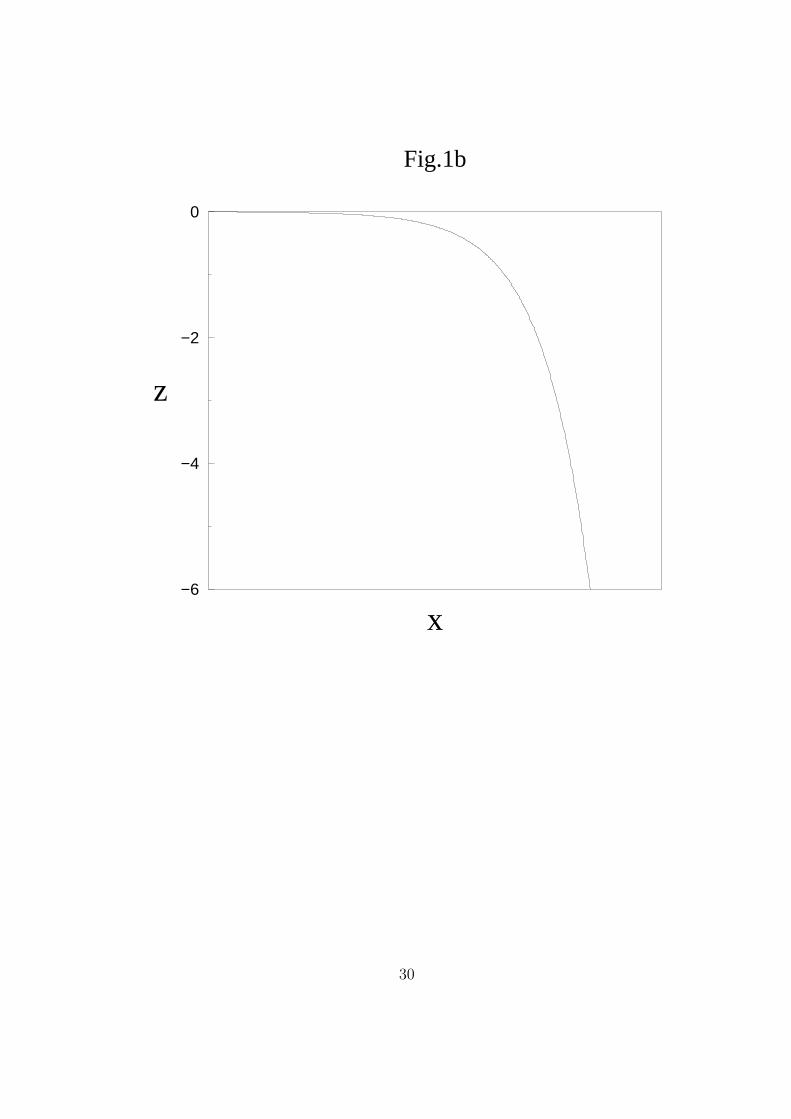
In what follows we consider the main flow with two different flow profiles

(Fig.1). The following standard (derivation can be found, for ex. in [10])

system of MHD equations holds for such flow

ut + (U+u)∇(U+u) =e

m∇φ (2.2a)

nt + n0∇u+∇(n(U+u)) = 0 (2.2b)

∆φ = 4πn (2.2c)

with the boundary condition at the “solid” edges of the electron flow (beam):

w(0) = 0 and w(−h) = 0, with h being the width of the beam. In (2.2) U is

the unperturbed flow velocity, and n0 is the unperturbed plasma concentra-

tion treated as a constant value; u=(u, v, w), n and φ are perturbations of

the velocity, electric potential and concentration ; e and m are the absolute

value of electron charge and mass.

Applying the multiple scale expansion proposed in [9] and used in [3] to

obtain equation (1.7) we introduce the following scaling of variables

u′ = u, v′ = v, w′ =w

ε, φ′ = φ, ξ = εz, µ = εy, θ = ε(x−Ut), τ = ε2t (2.3)

where the small parameter, ε = kh << 1, should be considered as an

expansion parameter. System (2.2) written up to the first order in ε is

nothing but the linearized version of (2.2), the same system written in the

second order of ε suggests the following ansatz for the velocity x-component

u = A(θ, µ, ξ, τ)U ′(z) (2.4)

We notice that this expression contains two disparate scales along z.

Amplitude A obeys one of the two equations corresponding to the flow

8

profiles pictured in Fig.1a and Fig.1b respectively.

Aτ + U ′AAθ − U2

U ′ G[Aθ] = 0 (2.5a)

Aτ + U ′AAθ +U2

U ′ G[Aθ] = 0 (2.5b)

where G is the integral operator

G[A(x,t)] =∫ ∫

k′ coth[k′h]A(x′,t) exp[ik′(x−x′)]∂x′∂k′

In the limiting case of a very thick electron beam (very deep layer of

fluid), h → ∞, G coincides with the operator in equation (1.7). By

a simple rescaling and nondimensionalization of the variables these two

equations can be written in the standard Benjamin-Ono form

Aτ + 6AAθ ± G[Aθ] = 0 (2.6)

The above equation (for any choice of sign) describes waves propagating

downstream slower then the main flow (upstream in the frame fixed on

the main flow). Physically, solitons of these equations are depressions in

the flow profile of the amplitude (“depth” of depressions) decreasing in the

z-direction. The direction of propagation (in the frame of reference fixed

on the main flow) coincides with the direction of the linear waves for the

surface flow in Fig.1a (minus sign) and is opposite to the direction of the

linear waves for the boundary flow in Fig.1b (plus sign).

The example of the electron flow considered above ( although of some-

what sketchy character) demonstrates the possibility of extending the ap-

plication of Shrira equation. Solitons of this equation have not been dis-

cussed in plasma applications, but taking into consideration the fact that

non-uniform flows are typical for plasmas, one could expect that algebraic

solitons might appear in such systems.

9

3 SOME REMARKS ABOUT THE STA-

BILITY OF SOLITONS WITH RESPECT

TO LONGITUDINAL PERTURBATIONS

In this section we want to briefly comment on the problem of stability of

the solitons of the (1+1) Benjamin-Ono equation. We shall consider the

Benjamin-Ono equation in the form

ut + 6uux + ∂2xH[u] = 0 (3.1)

which has the following well-known ”algebraic” soliton solution

u0 =2

3

S

1 + (Sx − Ωt)2, Ω = S2 (3.2)

where S is an arbitrary parameter defining velocity or amplitude of a soliton.

Let us consider the stability of the Benjamin-Ono solitons under the lon-

gitudinal perturbations. We proceed to linearize the Benjamin-Ono equa-

tion for

u = u0 + u(x − St, t) (3.3)

here u0 is the Benjamin-Ono soliton (3.2) and u - perturbation of a small

amplitude. Translational invariance necessitates that the gradient of the

soliton solution be an eigenfunction of the linearized problem.

The equation for the Fourier transform φ(q, ω) of the potential function

φ(x, t) (φ(x, t)x = u(x, t)) in the linearized problem can be shown to be

(∂2q − σ2)(−ωφ +

q

σφ + q |q| φ) + 4σ2qφ = 0 (3.5)

10

where σ = 1S. Equivalently, this equation could be written for function χ

satisfying φ = χqq − σ2χ

χqq −σ2 +

4σ1σ

+ |q| − ωq

χ = 0 (3.6)

Localized solution of this equation for perturbations with the stationary

amplitude (ω = 0) could be presented as

χ(q) = const · q(1 + σ |q|) exp[−σ |q|] (3.7)

which, in accordance with our above remark about translational invariance,

predictably gives a solution in the form of a soliton (3.2) after the inverse

Fourier transformation. In a more general case of the time-dependent per-

turbations we found a particular solution of (3.6) directly; it can be pre-

sented in the form

φ(x, t) = A(−iχ(k) +1 + 2χ(k)σ

θ − iσ) exp[−i(ωt + kx)] (3.8)

where A is an arbitrary constant amplitude of the perturbation.

Stability of the Benjamin-Ono solitons with respect to longitudinal per-

turbations is a well-known fact. Perturbation (3.8) does not destroy a

Benjamin-Ono soliton as a whole. It is worth noting that this perturbation

is not localized and contains a remote wave spreading to or from the soliton

(thus, probably, being not of much interest, but rather a mere curiousity).

However, we want to draw the reader’s attention to the way equation (3.6)

has been obtained. We shall use the same idea in the study of the (2 + 1)

analogue of the Benjamin-Ono equation.

11

4 TRANSVERSE INSTABILITY OF THE

SOLITONS OF (2+1) BENJAMIN-ONO

(SHRIRA) EQUATION

4.1 Solitons of the Shrira Equation

Equation

ut + cux + 6uux + G[ux] = 0 (4.1)

or its version in the frame fixed on the main flow

ut + 6uux + G[ux] = 0

clearly has plane solitons

u0 =2

3

S

1 + (Sx − Ωt)2(4.2)

as one of its solutions - as we mentioned before, on a restricted class of

functions, independent of y, the Shrira equation reduces to the Benjamin-

Ono equation. In what follows we want to consider a more general class of

solutions of (1.7) - solitons propagating at an arbitrary angle α to the main

flow

u0 =2

3

S

1 + (Sx − Ωt)2, Ω = S2 cos α (4.3)

The above dispersion relation contains cos α as a parameter which can

be included either into the expression for the velocity of wave propagation or

into the one for the amplitude. This allows us to consider the solitary wave

(4.3) either as a wave with a constant amplitude S travelling at a speed

S cos α or as a wave with a constant speed V = ΩS

having an amplitude

S = Vcos α

and a ”width” ∆ = cos αV

.

12

4.2 Transverse perturbations of the Shrira equation

We have mentioned that the Benjamin-Ono solitons (as well as Shrira soli-

tons propagating at a certain angle) are stable against the longitudinal

perturbations. However, the situation changes dramatically when we con-

sider the transverse perturbations. In this case, as we are about to show,

the solitons are unstable.

We shall find the equation which allows us to analyze instability. We

consider the perturbation u(ξ, η, t) = θ(ξ) exp[i(ωt + kηη)], with θ(ξ) being

a function with compact support, in the coordinate frame, oriented with

the soliton

ξ

η

=

cos α sin a

− sin α cos α

· x − ct

y

with c being the (rescaled) velocity of the main flow (at a fixed depth),

and linearize (4.1) obtaining an equation for θ (here θ, ξ, η should not be

confused with (2.3))

iωθ(ξ) = ∂x[cθ(ξ) − 6u0θ(ξ) − 1

2π(k2

η − ∂2ξ )×

×∫ 1[

(k′ξ)

2 + k2η

]1/2exp[ik′

ξ(ξ − ξ′)]θ(ξ′)∂k′ξ∂ξ′] (4.4)

∂x = cos α · ∂ξ − sin α · ikη

To cast this equation in a tractable form we perform the transformation

of Section 3, φ(q) =∫

θ(q′) exp[−σ |q − q′|]∂q′ where θ(q) is the Fourier

transform of θ(ξ). The new equation reads

φqq + [−σ2 − U ]φ = 0 (4.5)

13

U = − 4σ2

1 + σ[q2 + k2

η

]1/2 − Ωq−kη ·tan α

, Ω =σω

cos α, σ =

1

c

It is very interesting that this equation presents a Sturm-Liouville prob-

lem with the boundary conditions φ(±∞) = 0. Potential U is complex in

general (if spectral parameter Ω is complex).

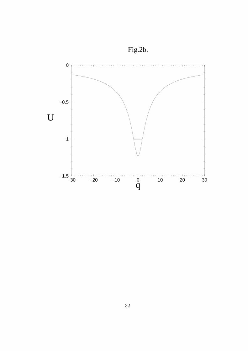
Some further analysis shows that there is an interesting connection be-

tween the structure of the levels in potential U and the instability of solitons.

This potential is real on the long-wave and short wave instability thresh-

olds, when the imaginary part of ω becomes equal to zero, and complex

in-between. A good illustration of the dynamics of the levels in such a po-

tential could be presented for zero angles of propagation. In this case the

potential consists of an even real part and an odd imaginary (see section 4.4

for more details). This means that the real part of an eigenfunction of (4.5)

is strictly even and the imaginary part is strictly odd, or vise versa. Thus,

the perturbation wave number being equal to 0 at the long-wave threshold,

the odd one-node eigenfunction of (4.5) is either strictly real or strictly imag-

inary and the energy E = −σ2 corresponds to the first energy level in the

potential. Further, as k increases the wave function becomes complex, but

turns even and either imaginary or real at the short-wave threshold where

the potential is more shallow (E = −σ2 is kept fixed) than at the long-wave

threshold. This is the wave function of the ground state (see Fig.2.). At

greater k the potential U has no level with E = −σ2, thus rendering the

instability impossible.

It should be noted that equation (4.4) was also obtained in [8]. Using the

asymptotic representation of the integrand in (4.4) the problem was restated

as an eigenvalue problem for small wave numbers and solved via Hirota’s

14

method. Thus obtained growth rate for the quasi-periodic non-linear wave

is given by γ2 = c2k2y −k2[(K −kx)

2 +k2y] where K is expressed through the

non-linearity parameter φ, K · σ = tanφ. This shows that the instability

region increases with the increasing non-linearity of the wave (decreasing

K · σ).

4.3 Transverse perturbations of Shrira solitons in long-

wave approximation. The critical angle

In this section we apply the small parameter expansion method to obtain

the growth rate of the ”inclined” solitons in the long-wave limit. For this we

expand the potential in equation (4.5) for small k (to simplify the notation

we put σ = 1)

U =−4

1 + |q|

1 +

− k2η

2|q| + Ωq

+ Ωkη tan αq2

1 + |q| +Ω2

q2

(1 + |q|)2

(4.6)

Equation (4.5) is reduced to the form

L[φ] ≡ (∂2q −1+

4

1 + |q|)φ =

4k2η

2|q| − 4Ωq− 4Ωkη tan α

q2

(1 + |q|)2−

4Ω2

q2

(1 + |q|)3

φ (4.7)

Further, we are looking for the complex frequency and the eigenfunction

as a series in a small parameter

Ω = εΩ1 + ε2Ω2 + ε3Ω3...

kη = εk1η + ε2k2

η + ε3k3η...

15

φ = φ0 + εφ1 + ε2φ2...

This will allow us to isolate consecutive orders in equation (4.7). Equat-

ing terms of different orders we get

L[φ0] = 0 (4.8a)

L[φ1] = − 4Ω1φ0

q(1 + |q|)2(4.8b)

L[φ2] = − 4Ω1φ1

q(1 + |q|)2− 4Ω2φ0

q(1 + |q|)2− 4Ω1k

1η tan α φ0

q2(1 + |q|)2+

+2(k1

η

)2φ0

|q| (1 + |q|)2− 4Ω2

1φ0

q2(1 + |q|)3(4.8c)

The first and the second of these equations can be easily solved to get

φ0 = q (1 + |q|) exp [− |q|]

φ1 = −Ω1 (exp [− |q|] + 2q(1 + q)η(q) exp [−q])

with η(q) being the step function.

We notice that because of equation (4.8a) and the self-adjoint property

of L the following condition should necessarily hold for all orders of φ

∫φ0L[φi]∂q = 0 (4.9)

Now, this condition for φ1 is satisfied as can be easily checked. The same

condition in the next order gives a non-trivial equation

∫φ0L[φ2]∂q = 0 =

(k1

η

)2

2+ Ω2

1 − 2k1η · tanα · Ω1 (4.10)

16

from which we obtain the dispersion relation in the long-wave limit (we drop

the ordering subscripts).

Ω = kη sin α ± i cos α

(k2

η

2− k2

η tan2 α

) 12

(4.11)

Of the special importance is the fact that this dispersion brings about the

existence of a critical angle. Two different scenarios for the growth rate are

separated by angle αc = arctan[

1√2

]. The growth rate itself is given by

γ = cos α · kη

21/2

(1 − 2 tan2 α

) 12 (4.12)

and for α > αcr it follows the tendency γkη

→ 0 as kη → 0. For α < αcr,

γkη

→ const.

It is worth noting that the case of α = 0 yeilds ω = 0 and γ = kη√2. This

result has been previously obtained in [6].

The above analysis shows that in the long-wave approximation the decay

rate grows linearly with the perturbation wave number.

4.4 Numerical Analysis of the Instability

The main result of this paper is the dependence of the instability growth

rate and the real frequency on the perturbation wave number for several

angles of propagation. To this end we procede to analyze equation (4.5)

numerically.

To limit the range of the independent variable in (4.5) we used the

following substitution

x =2

πarctan(q) (4.10)

Taking into account the fact that in the most general case of an arbitrary

angle of propagation the potential in (4.5) is complex, substitution (4.10)

17

transforms the Sturm-Liouville equation (4.5) into an equation for a complex

eigenfunction φ(x)

4 cos4(πx2

)

π2φ′′ − 4 cos4(πx

2) tan(πx

2)

πφ′ +

(−σ2 − U(x)

)φ = 0 (4.11)

U(x) =−4σ2

1 + σ[tan(πx

2)2 + k2

η

]1/2 − Ωtan(πx

2)−kη ·tan α

We discretize this equation using the standard two-point approxima-

tion for the first derivative and three-point approximation for the second

derivative, obtaining a linear problem for the vector of point-values of the

complex eigenfunction. This problem, of the form Ae = 0 with zero bound-

ary conditions at x = 1 and x = −1, has a non-trivial solution iff complex

det(A)(ω, γ, k) = 0 with ω = <[Ω] and γ = =[Ω]. We solve this equation

for each value of k using the standard 2 − D globally convergent Newton

method with line search and backtracking [12].

To test the viability of the method we try it on the Sturm-Liouville

problem with the soliton-like complex potential

U(x) = −ω sech2(tan

(πx

2

))− iγ sech2

(tan

(πx

2

))

The real part of this potential is the famous attracting KDV-soliton

appearing in the direct problem for the KDV equation. It is a well-known

fact that the Sturm-Liouville problem with such complex potential and zero-

boundary conditions posses eigenvalue λ = −1 for ω = n(n + 1), γ = 0.

These values of ω and λ correspond to the (n − 1)st energy level in the

soliton well (see, for ex., [13]).

We ran our root-finding procedure for several discretizations of the in-

terval (−1, 1). Here we include the results of convergence of ω and γ to

18

the required values for two initial approximation: ω = 0.5, γ = 1.0 and

ω = 31.0, γ = 2.0. We expect the first set of data converge to ω = 2.0,

γ = 0.0 (n = 1) and the second to ω = 30.0, γ = 0.0 (n = 5) . The values

of ω, γ (rounded up to 3 significant figures) and the number of iterations

in Newton root-finding are summarized in Tables 1 and 2. For this test the

convergence criterion on the function value in Newton procedure was kept

at 1.0E − 14, the step convergence criterion at 1.0E − 16 and criterion of

convergence on a spurious minimum at 1.0E − 15. For all discretizations

Newton root-finding was terminated by step converegnce.

As a further demonstration of the method we include the convergence

results of our algorithm for various discretizations of the Sturm-Liouville

problem with potential (4.11). The results for for angle α = π6

and per-

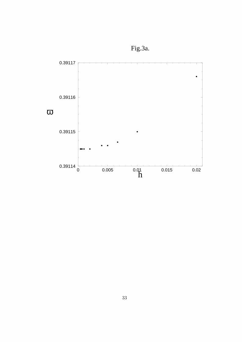
turbation wave number k = 1.0 are given in Table 3 and Fig.3. The first

column is the value of the step used in the discretization of the equation,

the second and the fourth columns are the obtained values of ω and γ, the

third and the fifth columns show the difference of ω and γ values for two

consecutive discretizations. All differences are rounded up to 3 significant

figures. The convergence is obviously superlinear and probably quadratic

as it should be expected for a second-order scheme.

Thus tested algorithm was used to compute the dispersion curves of the

perturbed Shrira equation. The obtained dependencies are pictured in Fig.4.

These curves do show the expected behavior: solitons propagating along the

flow are the most unstable, instability decreases with the increasing angle

of propagation eventually disappearing for perpendicular solitons.

It should be noted that the obtained instability growth rate dependence

on the transverse perturbation wave number is quite similar to those typical

19

of many well-known classical non-linear wave models such as KdV, KP and

NSE. If a soliton described by this model is unstable against the transverse

perturbation then, at the long-wave end of the instability range, growth

rate increases with increasing wave number, further, for shorter waves the

dynamics is stabilized when the wave-length is of the order of characteristic

length defined by dispersion.

In contrast to the earlier obtained results [8], there are no multiple zones

of instability within the instability range, rather, there exists a single uni-

versal zone of instability, and the short wave threshold turns out constant

for all angles of soliton inclination.

In an attempt to justify our predictions of Section 4.3 for the long-wave

growth rate behavior we used our numerical scheme for small k and for

two angles, above and below the predicted critical angle. Results, shown in

Fig.5, do confirm the existence of a critical angle, separating two types of

behavior. A remark, however, is in order: we were not able to implement the

algorithm all the way to k = 0. For very small k and Ω the potential becomes

very irregular and our numerical scheme produces (spurious) oscilations in

the dispersion curves. Despite of this, tendencies of γk

for angles above and

below critical are obviously in accord with predictions of Section 4.3.

4.5 Stability of Solitons Propagating Perpendicular to

the Main Flow

Let us consider ”perpendicular” solitons - solitons moving at angle π2

to the

main flow. In accordance with two approaches to a solitary wave outlined

in Section 4.1, these ”perpendicular” waves could be viewed as waves with

20

either amplitude or velocity independent of the angle. The former are the

waves with the phase velocity V = ΩS

= S cos α = S cos π2

= 0

u0 =2

3

S

1 + (Sξ)2(4.12)

the latter are the δ-waves with the amplitude S = Vcos α

→ ∞ for α → π2,

that is

u0 =2

3πδ(ξ − V t) (4.13)

We limit our consideration to the long-wave case when equation (4.5)

could be rewritten as

φqq + [−1 − U(q, α)]φ = 0 (4.14)

U = − 4

1 + |q| − ν, ν =

[Ω cos α

kη

]kη→0

where we have put for simplicity σ = 1 which is equivalent to the change

σ · q → q. Matching relatively self-suggesting solutions of (4.14) and their

derivatives for negative and positive values of q we could find two even

solutions

φ0 = (ν0 + |q|) · (1 + ν0 + |q|) exp[− |q|], ν0 =1 +

√5

2(4.15a)

φ2 = (ν2 + |q|) · (1 + ν2 + |q|) exp[− |q|], ν2 =1 −√

5

2(4.15b)

and two odd

φ1 = q · (1 + |q|) exp[− |q|], ν1 = 0 (4.15c)

φ3 = q · (1 − |q|) exp[− |q|], ν3 = −1 (4.15d)

It can be seen that the spectral parameter ν0 corresponds to an eigen-

function without zeros, that is an eigenfunction of the ground state (level)

21

of the potential U ; parameter ν1 corresponds to the one-node function of

the first state; parameter ν2 corresponds to the eigenfunction of the second

state with two nodes; and parameter ν3 - to the eigenfunction of the third

level with three nodes. The depth of the potential is different for these

parameter values, while the energy of the corresponding state is constant

and equal to −1. Of the special importance is the fact that all parameter

values are real. This means that for the solitons (4.12)

[kηνi]kη→0 = [Ω cos α]α→π2

= ω (4.16)

the perturbation frequency is real and the four perturbation modes (4.15)

are stable . This is in line with (4.12) since the instability growth rate should

go to zero faster than kη for angle larger than the critical, and π2

is certainly

larger than αcr.

If we think of the ” perpendicular” solitons as the δ-solitons we get

νi

[kη

cos α

]kη→0,α→π

2

= ω

The δ-solitons are also stable with respect to the transverse perturba-

tions. This perturbation is not stationary in the limiting case of[

kη

cos α

]kη→0,α→π

2

→const. We want to note, however, that the consideration of solitons with

a vary large (in the limit, infinitely large) amplitude within the framework

of the model is somewhat awkward. The appearance of the δ-solitons is an

artifact of our two-sided approach to incorporating cos α into the dispersion

relation (Section 4.1); thus thinking of the ”inclined” solitons as waves with

the amplitude independent of the angle and varying velocity should be more

natural.

22

5 CONCLUSION

We have considered stable and unstable dynamics of solitons in boundary

and surface layers of shear hydrodynamic flows. Several aforementioned

results are worth emphasizing.

First, the value of the short-wave threshold of the longitudinal pertur-

bation of the solitons turned out to be constant and independent of the

angle of propagation of the soliton with respect to the main shear flow. We

determined this value numerically to be kth

c= 2.2625 ± 0.0005 where c is

the velocity of the main flow.

Second, using numerical methods we found the dependence of the insta-

bility growth rate and the real frequency on the perturbation wave number

for several angles of propagation. Numerical calculations show that the

maximum of the growth rate decreases with the growth of the propagation

angle and becomes equal zero for π2. For a fixed angle both the growth

rate and the real frequency monotonously grow with the perturbation wave

number to a certain maximum, then monotonously decrease and become

equal zero at the short-wave threshold.

Third, solitons propagating at a right angle to the main flow are known

to be stable. We have found four stable transverse perturbation modes for

such waves.

Lastly, analytic considerations allow us to predict the character of the

growth rate dependency on the propagation angle for long waves. We have

shown that there should exist a critical angle of propagation in the long-

wave limit which serves as a border between two different behaviors of the

growth rate: γkη

→ 0 for α > αcr and γkη

→ const for α < αcr.

23

6 REFERENCES

References

[1] T. B. Benjamin. Internal waves of permanent form in fluids of great

depth, J. Fluid Mech., 1967, vol. 29, #3, p. 559.

[2] H. Ono. Algebraic solitary waves in stratified fluids, J. Phys. Soc. Jap.,

1975, vol. 39, #4, p. 1082.

[3] V. I. Shrira. On surface waves in the upper quasi-uniform ocean layer.

Dokl. Akad. Nauk SSSR, 1989, vol. 308, #3, p. 732.

[4] R. Hirota. Lecture Notes in Physics, 1976, vol. 515.

[5] J. Satsuma and Y. Ishimori. Periodic wave and rational soliton solutions

of the Benjamin-Ono equation, J. Phys. Soc. Jap., 1979, vol. 46, #2, p.

681.

[6] A. N. Dyachenko and E. A. Kuznetsov. Instability and self-focusing of

solitons in the boundary layer, JETPh Letters, 1994, vol. 59, #2, p.

108.

[7] L. A. Abramyan, Yu. A. Stepanyants, V. I. Shrira. Multidimensional

solitons in shear flows of the boundary-layer type, Sov. Phys. Dokl.,

1992, vol. 37, #12, p. 575.

[8] D. A. Pelinovsky, Yu. A. Stepanyants. Self-focusing instability of soli-

tons in shear flows. JETPh, 1994, vol. 78, #6, p. 883.

24

[9] Y. Serizawa, T. Wantanabe, M. B. Chaudhry, and K. Nishikawa. J. A

numerical method for eigenvalue problems of integral equations, J. Phys.

Soc. Jap., 1983, vol 52, #1, p. 28.

[10] A. B. Mikhailovskii. Theory of Plasma Instabilities, New York, 1975.

[11] V. I. Petviashvili. Solitary Waves in Plasmas and in the Atmosphere,

Philadelphia, 1992.

[12] W. H. Press et al. Numerical Recipes in Fortran. The Art of Scientific

Computing, Cambridge, 1992.

[13] G. L. Lamb Elements of Soliton Theory, New York: Wiley, 1980.

25

7 List of figure captions

1. Fig.1a. Example of a free surface flow profile. Fig.1b. Example of a

boundary flow profile.

2. Fig.2a. Energy levels at the long-wave instability threshold: the ground

state (solid line) and the first ”excited” state (dashed line). Fig.2b. Energy

levels at the short-wave instability threshold: the ground state (solid line).

3. Fig.3a. ω as a function of discretization step. α = π6, k = 1.0. Fig.3b. γ

as a function of discretization step. α = π6, k = 1.0.

4. Fig.4a. Dependence of the real frequency, ω, on wave number, k, for

several angles of propagation (in radians, top to bottom): π4, 0.62, 0.60, π

6, π

8,

π16

, π24

. (Remark : frequency curve for angle 0 coincides with the horizontal

axis). Fig.4b. Dependence of the growth rate, γ, on wave number, k, for

several angles of propogation (in radians, top to bottom): 0, π24

, π16

, π8, π

6,

0.60, 0.62, π4.

5. Fig.5. Dependence of the growth rate divided by the wave number, Γ,

on the wave number, k, for two angles of propagation, above and below

critical, π6

(upper curve) and π4

(lower curve).

26

8 Tables

number of points ω − n(n + 1) γ number of iterations

100 −8.07E − 04 −8.90E − 07 11

500 −3.36E − 05 −7.50E − 07 10

1000 −9.37E − 06 −7.51E − 07 12

2000 −3.31E − 06 −7.46E − 07 11

3000 −2.20E − 06 −7.51E − 07 15

4000 −1.81E − 06 −7.54E − 07 16

Tab.1. Values of ω and γ for initial data ω = 0.5 and γ = 1.0

number of points ω − n(n + 1) γ number of iterations

100 2.76 −7.63E − 07 7

500 −1.21E − 02 4.86E − 07 7

1000 −3.05E − 03 4.72E − 07 8

2000 −7.77E − 04 4.39E − 07 7

3000 −3.56E − 04 4.32E − 07 7

4000 −2.08E − 04 4.30E − 07 8

Tab.2. Values of ω and γ for initial data ω = 31.0 and γ = 2.0

27

hi ωi ωi − ωi−1 γi γi − γi−1

2.0E − 02 0.391165562 0.338741227

4.0E − 03 0.391145659 −1.99E − 5 0.339520253 7.79E − 4

2.0E − 03 0.391144974 −6.85E − 7 0.339544804 2.45E − 5

1.0E − 03 0.391144802 −1.72E − 7 0.339550943 6.12E − 6

6.6(6)E − 04 0.391144769 −3.3E − 8 0.339552079 1.14E − 6

5.0E − 04 0.391144758 −1.1E − 8 0.339552477 3.98E − 7

4.0E − 04 0.391144753 −5.0E − 9 0.339552661 1.84E − 7

3.51E − 04 0.39114475 −3.0E − 9 0.339552737 7.6E − 8

Tab.3. Convergence of the real frequency and the growth rate for several

discretizations of (4.11).

28

0 0.2 0.4 0.6 0.8 1 1.2x

−6

−4

−2

0

z

Fig.1a

29

−8 −6 −4 −2 0x

−6

−4

−2

0

z

Fig.1b

30

−30 −20 −10 0 10 20 30q

−4.5

−3.5

−2.5

−1.5

−0.5

U

Fig.2a.

31

−30 −20 −10 0 10 20 30q

−1.5

−1

−0.5

0

U

Fig.2b.

32

0 0.005 0.01 0.015 0.02h

0.39114

0.39115

0.39116

0.39117

ω

Fig.3a.

33

0 0.005 0.01 0.015 0.02h

0.3385

0.3387

0.3389

0.3391

0.3393

0.3395

0.3397

0.3399

γ

Fig.3b.

34

0 0.5 1 1.5 2k

0

0.1

0.2

0.3

0.4

0.5

0.6

0.7

0.8

ω

Fig.4a.

35

0 0.5 1 1.5 2k

0

0.1

0.2

0.3

0.4

0.5

γ

Fig.4b.

36

0 0.1 0.2 0.3k

0

0.1

0.2

0.3

0.4

Γ

Fig. 5.

37