On the importance of initialization and momentum …hinton/absps/momentum.pdfOn the importance of initialization and momentum in deep learning certain situations. In particular, for

On the importance of initialization and momentum in deep learning

Ilya Sutskever1 [email protected] Martens [email protected] Dahl [email protected] Hinton [email protected]

Abstract

Deep and recurrent neural networks (DNNsand RNNs respectively) are powerful mod-els that were considered to be almost impos-sible to train using stochastic gradient de-scent with momentum. In this paper, weshow that when stochastic gradient descentwith momentum uses a well-designed randominitialization and a particular type of slowlyincreasing schedule for the momentum pa-rameter, it can train both DNNs and RNNs(on datasets with long-term dependencies) tolevels of performance that were previouslyachievable only with Hessian-Free optimiza-tion. We find that both the initializationand the momentum are crucial since poorlyinitialized networks cannot be trained withmomentum and well-initialized networks per-form markedly worse when the momentum isabsent or poorly tuned.

Our success training these models suggeststhat previous attempts to train deep and re-current neural networks from random initial-izations have likely failed due to poor ini-tialization schemes. Furthermore, carefullytuned momentum methods suffice for dealingwith the curvature issues in deep and recur-rent network training objectives without theneed for sophisticated second-order methods.

1. Introduction

Deep and recurrent neural networks (DNNs andRNNs, respectively) are powerful models that achievehigh performance on difficult pattern recognition prob-lems in vision, and speech (Krizhevsky et al., 2012;Hinton et al., 2012; Dahl et al., 2012; Graves, 2012).

Although their representational power is appealing,the difficulty of training DNNs has prevented their

Proceedings of the 30 th International Conference on Ma-chine Learning, Atlanta, Georgia, USA, 2013. JMLR:W&CP volume 28. Copyright 2013 by the author(s).

widepread use until fairly recently. DNNs becamethe subject of renewed attention following the workof Hinton et al. (2006) who introduced the idea ofgreedy layerwise pre-training. This approach has sincebranched into a family of methods (Bengio et al.,2007), all of which train the layers of the DNN in asequence using an auxiliary objective and then “fine-tune” the entire network with standard optimizationmethods such as stochastic gradient descent (SGD).More recently, Martens (2010) attracted considerableattention by showing that a type of truncated-Newtonmethod called Hessian-free Optimization (HF) is capa-ble of training DNNs from certain random initializa-tions without the use of pre-training, and can achievelower errors for the various auto-encoding tasks con-sidered by Hinton & Salakhutdinov (2006).

Recurrent neural networks (RNNs), the temporal ana-logue of DNNs, are highly expressive sequence mod-els that can model complex sequence relationships.They can be viewed as very deep neural networksthat have a “layer” for each time-step with parame-ter sharing across the layers and, for this reason, theyare considered to be even harder to train than DNNs.Recently, Martens & Sutskever (2011) showed thatthe HF method of Martens (2010) could effectivelytrain RNNs on artificial problems that exhibit verylong-range dependencies (Hochreiter & Schmidhuber,1997). Without resorting to special types of memoryunits, these problems were considered to be impossi-bly difficult for first-order optimization methods dueto the well known vanishing gradient problem (Bengioet al., 1994). Sutskever et al. (2011) and later Mikolovet al. (2012) then applied HF to train RNNs to per-form character-level language modeling and achievedexcellent results.

Recently, several results have appeared to challengethe commonly held belief that simpler first-ordermethods are incapable of learning deep models fromrandom initializations. The work of Glorot & Ben-gio (2010), Mohamed et al. (2012), and Krizhevskyet al. (2012) reported little difficulty training neuralnetworks with depths up to 8 from certain well-chosen

1Work was done while the author was at the Universityof Toronto.


random initializations. Notably, Chapelle & Erhan(2011) used the random initialization of Glorot & Ben-gio (2010) and SGD to train the 11-layer autoencoderof Hinton & Salakhutdinov (2006), and were able tosurpass the results reported by Hinton & Salakhutdi-nov (2006). While these results still fall short of thosereported in Martens (2010) for the same tasks, theyindicate that learning deep networks is not nearly ashard as was previously believed.

The first contribution of this paper is a much morethorough investigation of the difficulty of training deepand temporal networks than has been previously done.In particular, we study the effectiveness of SGD whencombined with well-chosen initialization schemes andvarious forms of momentum-based acceleration. Weshow that while a definite performance gap seems toexist between plain SGD and HF on certain deep andtemporal learning problems, this gap can be elimi-nated or nearly eliminated (depending on the prob-lem) by careful use of classical momentum methodsor Nesterov’s accelerated gradient. In particular, weshow how certain carefully designed schedules for theconstant of momentum µ, which are inspired by var-ious theoretical convergence-rate theorems (Nesterov,1983; 2003), produce results that even surpass those re-ported by Martens (2010) on certain deep-autencodertraining tasks. For the long-term dependency RNNtasks examined in Martens & Sutskever (2011), whichfirst appeared in Hochreiter & Schmidhuber (1997),we obtain results that fall just short of those reportedin that work, where a considerably more complex ap-proach was used.

Our results are particularly surprising given that mo-mentum and its use within neural network optimiza-tion has been studied extensively before, such as in thework of Orr (1996), and it was never found to have suchan important role in deep learning. One explanation isthat previous theoretical analyses and practical bench-marking focused on local convergence in the stochasticsetting, which is more of an estimation problem thanan optimization one (Bottou & LeCun, 2004). In deeplearning problems this final phase of learning is notnearly as long or important as the initial “transientphase” (Darken & Moody, 1993), where a better ar-gument can be made for the beneficial effects of mo-mentum.

In addition to the inappropriate focus on purely localconvergence rates, we believe that the use of poorly de-signed standard random initializations, such as thosein Hinton & Salakhutdinov (2006), and suboptimalmeta-parameter schedules (for the momentum con-stant in particular) has hampered the discovery of thetrue effectiveness of first-order momentum methods indeep learning. We carefully avoid both of these pit-falls in our experiments and provide a simple to under-stand and easy to use framework for deep learning that

is surprisingly effective and can be naturally combinedwith techniques such as those in Raiko et al. (2011).

We will also discuss the links between classical mo-mentum and Nesterov’s accelerated gradient method(which has been the subject of much recent study inconvex optimization theory), arguing that the lattercan be viewed as a simple modification of the formerwhich increases stability, and can sometimes provide adistinct improvement in performance we demonstratedin our experiments. We perform a theoretical analysiswhich makes clear the precise difference in local be-havior of these two algorithms. Additionally, we showhow HF employs what can be viewed as a type of “mo-mentum” through its use of special initializations toconjugate gradient that are computed from the up-date at the previous time-step. We use this propertyto develop a more momentum-like version of HF whichcombines some of the advantages of both methods tofurther improve on the results of Martens (2010).

2. Momentum and Nesterov’sAccelerated Gradient

The momentum method (Polyak, 1964), which we referto as classical momentum (CM), is a technique for ac-celerating gradient descent that accumulates a velocityvector in directions of persistent reduction in the ob-jective across iterations. Given an objective functionf(θ) to be minimized, classical momentum is given by:

vt+1 = µvt − ε∇f(θt) (1)

θt+1 = θt + vt+1 (2)

where ε > 0 is the learning rate, µ ∈ [0, 1] is the mo-mentum coefficient, and ∇f(θt) is the gradient at θt.

Since directions d of low-curvature have, by defini-tion, slower local change in their rate of reduction (i.e.,d>∇f), they will tend to persist across iterations andbe amplified by CM. Second-order methods also am-plify steps in low-curvature directions, but instead ofaccumulating changes they reweight the update alongeach eigen-direction of the curvature matrix by the in-verse of the associated curvature. And just as second-order methods enjoy improved local convergence rates,Polyak (1964) showed that CM can considerably accel-

erate convergence to a local minimum, requiring√R-

times fewer iterations than steepest descent to reachthe same level of accuracy, where R is the conditionnumber of the curvature at the minimum and µ is setto (√R− 1)/(

√R+ 1).

Nesterov’s Accelerated Gradient (abbrv. NAG; Nes-terov, 1983) has been the subject of much recent at-tention by the convex optimization community (e.g.,Cotter et al., 2011; Lan, 2010). Like momentum,NAG is a first-order optimization method with betterconvergence rate guarantee than gradient descent in


certain situations. In particular, for general smooth(non-strongly) convex functions and a deterministicgradient, NAG achieves a global convergence rate ofO(1/T 2) (versus the O(1/T ) of gradient descent), withconstant proportional to the Lipschitz coefficient of thederivative and the squared Euclidean distance to thesolution. While NAG is not typically thought of as atype of momentum, it indeed turns out to be closely re-lated to classical momentum, differing only in the pre-cise update of the velocity vector v, the significance ofwhich we will discuss in the next sub-section. Specifi-cally, as shown in the appendix, the NAG update maybe rewritten as:

vt+1 = µvt − ε∇f(θt + µvt) (3)

θt+1 = θt + vt+1 (4)

While the classical convergence theories for both meth-ods rely on noiseless gradient estimates (i.e., notstochastic), with some care in practice they are bothapplicable to the stochastic setting. However, the the-ory predicts that any advantages in terms of asymp-totic local rate of convergence will be lost (Orr, 1996;Wiegerinck et al., 1999), a result also confirmed in ex-periments (LeCun et al., 1998). For these reasons,interest in momentum methods diminished after theyhad received substantial attention in the 90’s. And be-cause of this apparent incompatibility with stochasticoptimization, some authors even discourage using mo-mentum or downplay its potential advantages (LeCunet al., 1998).

However, while local convergence is all that mattersin terms of asymptotic convergence rates (and on cer-tain very simple/shallow neural network optimizationproblems it may even dominate the total learningtime), in practice, the “transient phase” of convergence(Darken & Moody, 1993), which occurs before fine lo-cal convergence sets in, seems to matter a lot morefor optimizing deep neural networks. In this transientphase of learning, directions of reduction in the ob-jective tend to persist across many successive gradientestimates and are not completely swamped by noise.

Although the transient phase of learning is most no-ticeable in training deep learning models, it is still no-ticeable in convex objectives. The convergence rateof stochastic gradient descent on smooth convex func-tions is given by O(L/T + σ/

√T ), where σ is the

variance in the gradient estimate and L is the Lip-shits coefficient of ∇f . In contrast, the convergencerate of an accelerated gradient method of Lan (2010)(which is related to but different from NAG, in thatit combines Nesterov style momentum with dual aver-aging) is O(L/T 2 + σ/

√T ). Thus, for convex objec-

tives, momentum-based methods will outperform SGDin the early or transient stages of the optimizationwhere L/T is the dominant term. However, the twomethods will be equally effective during the final stages

Figure 1. (Top) Classical Momentum (Bottom) Nes-terov Accelerated Gradient

of the optimization where σ/√T is the dominant term

(i.e., when the optimization problem resembles an es-timation one).

2.1. The Relationship between CM and NAG

From Eqs. 1-4 we see that both CM and NAG computethe new velocity by applying a gradient-based correc-tion to the previous velocity vector (which is decayed),and then add the velocity to θt. But while CM com-putes the gradient update from the current positionθt, NAG first performs a partial update to θt, comput-ing θt + µvt, which is similar to θt+1, but missing theas yet unknown correction. This benign-looking dif-ference seems to allow NAG to change v in a quickerand more responsive way, letting it behave more sta-bly than CM in many situations, especially for highervalues of µ.

Indeed, consider the situation where the addition ofµvt results in an immediate undesirable increase inthe objective f . The gradient correction to the ve-locity vt is computed at position θt + µvt and if µvtis indeed a poor update, then ∇f(θt + µvt) will pointback towards θt more strongly than ∇f(θt) does, thusproviding a larger and more timely correction to vtthan CM. See fig. 1 for a diagram which illustratesthis phenomenon geometrically. While each iterationof NAG may only be slightly more effective than CMat correcting a large and inappropriate velocity, thisdifference in effectiveness may compound as the al-gorithms iterate. To demonstrate this compounding,we applied both NAG and CM to a two-dimensionaloblong quadratic objective, both with the same mo-mentum and learning rate constants (see fig. 2 in theappendix). While the optimization path taken by CMexhibits large oscillations along the high-curvature ver-tical direction, NAG is able to avoid these oscillationsalmost entirely, confirming the intuition that it is muchmore effective than CM at decelerating over the courseof multiple iterations, thus making NAG more tolerantof large values of µ compared to CM.

In order to make these intuitions more rigorous and


help quantify precisely the way in which CM andNAG differ, we analyzed the behavior of each methodwhen applied to a positive definite quadratic objectiveq(x) = x>Ax/2 + b>x. We can think of CM and NAGas operating independently over the different eigendi-rections of A. NAG operates along any one of thesedirections equivalently to CM, except with an effectivevalue of µ that is given by µ(1 − λε), where λ is theassociated eigenvalue/curvature.

The first step of this argument is to reparameterizeq(x) in terms of the coefficients of x under the basisof eigenvectors of A. Note that since A = U>DU fora diagonal D and orthonormal U (as A is symmetric),we can reparameterize q(x) by the matrix transformU and optimize y = Ux using the objective p(y) ≡q(x) = q(U>y) = y>U

(U>DU

)U>y/2 + b>U>y =

y>Dy/2 + c>y, where c = Ub. We can further rewritep as p(y) =

∑ni=1[p]i([y]i), where [p]i(t) = λit

2/2+[c]itand λi > 0 are the diagonal entries of D (and thusthe eigenvalues of A) and correspond to the curva-ture along the associated eigenvector directions. Asshown in the appendix (Proposition 6.1), both CMand NAG, being first-order methods, are “invariant”to these kinds of reparameterizations by orthonormaltransformations such as U . Thus when analyzing thebehavior of either algorithm applied to q(x), we can in-stead apply them to p(y), and transform the resultingsequence of iterates back to the default parameteriza-tion (via multiplication by U−1 = U>).

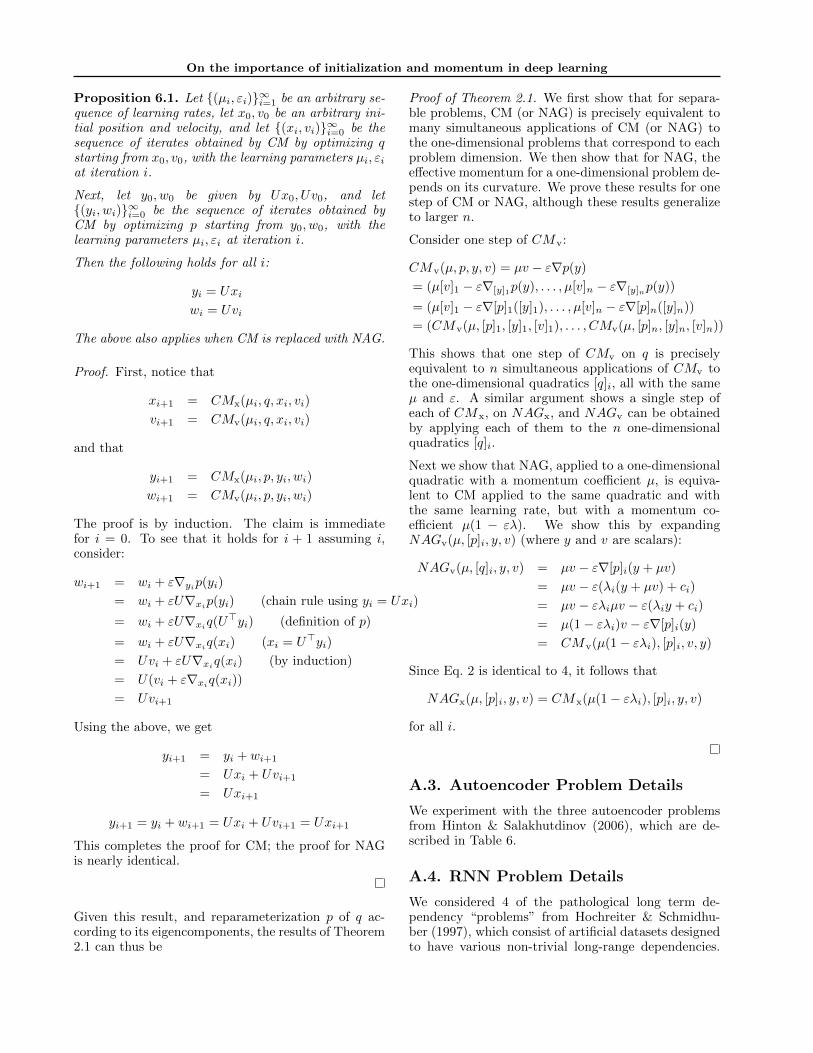
Theorem 2.1. Let p(y) =∑n

i=1[p]i([y]i) such that[p]i(t) = λit

2/2 + cit. Let ε be arbitrary and fixed.Denote by CMx(µ, p, y, v) and CMv(µ, p, y, v) the pa-rameter vector and the velocity vector respectively, ob-tained by applying one step of CM (i.e., Eq. 1 and thenEq. 2) to the function p at point y, with velocity v,momentum coefficient µ, and learning rate ε. DefineNAGx and NAGv analogously. Then the followingholds for z ∈ {x, v}:

CM z(µ, p, y, v) =

CM z(µ, [p]1, [y]1, [v]1)...

CM z(µ, [p]n, [y]n, [v]n)

NAGz(µ, p, y, v) =

CM z(µ(1− λ1ε), [p]1, [y]1, [v]1)...

CM z(µ(1− λnε), [p]n, [y]n, [v]n)

Proof. See the appendix.

The theorem has several implications. First, CM andNAG become equivalent when ε is small (when ελ� 1for every eigenvalue λ of A), so NAG and CM aredistinct only when ε is reasonably large. When ε isrelatively large, NAG uses smaller effective momentumfor the high-curvature eigen-directions, which prevents

oscillations (or divergence) and thus allows the use ofa larger µ than is possible with CM for a given ε.

3. Deep Autoencoders

The aim of our experiments is three-fold. First, toinvestigate the attainable performance of stochasticmomentum methods on deep autoencoders startingfrom well-designed random initializations; second, toexplore the importance and effect of the schedule forthe momentum parameter µ assuming an optimal fixedchoice of the learning rate ε; and third, to compare theperformance of NAG versus CM.

For our experiments with feed-forward nets, we fo-cused on training the three deep autoencoder prob-lems described in Hinton & Salakhutdinov (2006) (seesec. A.2 for details). The task of the neural net-work autoencoder is to reconstruct its own input sub-ject to the constraint that one of its hidden layers isof low-dimension. This “bottleneck” layer acts as alow-dimensional code for the original input, similar toother dimensionality reduction techniques like Princi-ple Component Analysis (PCA). These autoencodersare some of the deepest neural networks with pub-lished results, ranging between 7 and 11 layers, andhave become a standard benchmarking problem (e.g.,Martens, 2010; Glorot & Bengio, 2010; Chapelle & Er-han, 2011; Raiko et al., 2011). See the appendix formore details.

Because the focus of this study is on optimization, weonly report training errors in our experiments. Testerror depends strongly on the amount of overfitting inthese problems, which in turn depends on the type andamount of regularization used during training. Whileregularization is an issue of vital importance when de-signing systems of practical utility, it is outside thescope of our discussion. And while it could be ob-jected that the gains achieved using better optimiza-tion methods are only due to more exact fitting of thetraining set in a manner that does not generalize, thisis simply not the case in these problems, where under-trained solutions are known to perform poorly on boththe training and test sets (underfitting).

The networks we trained used the standard sigmoidnonlinearity and were initialized using the “sparse ini-tialization” technique (SI) of Martens (2010) that isdescribed in sec. 3.1. Each trial consists of 750,000parameter updates on minibatches of size 200. No reg-ularization is used. The schedule for µ was given bythe following formula:

µt = min(1− 2−1−log2(bt/250c+1), µmax ) (5)

where µmax was chosen from{0.999, 0.995, 0.99, 0.9, 0}. This schedule was mo-tivated by Nesterov (1983) who advocates using whatamounts to µt = 1−3/(t+5) after some manipulation


task 0(SGD) 0.9N 0.99N 0.995N 0.999N 0.9M 0.99M 0.995M 0.999M SGDC HF† HF∗

Curves 0.48 0.16 0.096 0.091 0.074 0.15 0.10 0.10 0.10 0.16 0.058 0.11Mnist 2.1 1.0 0.73 0.75 0.80 1.0 0.77 0.84 0.90 0.9 0.69 1.40Faces 36.4 14.2 8.5 7.8 7.7 15.3 8.7 8.3 9.3 NA 7.5 12.0

Table 1. The table reports the squared errors on the problems for each combination of µmax and a momentum type(NAG, CM). When µmax is 0 the choice of NAG vs CM is of no consequence so the training errors are presented in asingle column. For each choice of µmax , the highest-performing learning rate is used. The column SGDC lists the results ofChapelle & Erhan (2011) who used 1.7M SGD steps and tanh networks. The column HF† lists the results of HF withoutL2 regularization, as described in sec. 5; and the column HF∗ lists the results of Martens (2010).

problem before afterCurves 0.096 0.074Mnist 1.20 0.73Faces 10.83 7.7

Table 2. The effect of low-momentum finetuning for NAG.The table shows the training squared errors before andafter the momentum coefficient is reduced. During the pri-mary (“transient”) phase of learning we used the optimalmomentum and learning rates.

(see appendix), and by Nesterov (2003) who advocatesa constant µt that depends on (essentially) the con-dition number. The constant µt achieves exponentialconvergence on strongly convex functions, while the1−3/(t+5) schedule is appropriate when the functionis not strongly convex. The schedule of Eq. 5 blendsthese proposals. For each choice of µmax , we reportthe learning rate that achieved the best training error.Given the schedule for µ, the learning rate ε waschosen from {0.05, 0.01, 0.005, 0.001, 0.0005, 0.0001}in order to achieve the lowest final error training errorafter our fixed number of updates.

Table 1 summarizes the results of these experiments.It shows that NAG achieves the lowest publishedresults on this set of problems, including those ofMartens (2010). It also shows that larger values ofµmax tend to achieve better performance and thatNAG usually outperforms CM, especially when µmax

is 0.995 and 0.999. Most surprising and importantly,the results demonstrate that NAG can achieve resultsthat are comparable with some of the best HF resultsfor training deep autoencoders. Note that the previ-ously published results on HF used L2 regularization,so they cannot be directly compared. However, thetable also includes experiments we performed with animproved version of HF (see sec. 2.1) where weightdecay was removed towards the end of training.

We found it beneficial to reduce µ to 0.9 (unless µis 0, in which case it is unchanged) during the final1000 parameter updates of the optimization withoutreducing the learning rate, as shown in Table 2. Itappears that reducing the momentum coefficient al-lows for finer convergence to take place whereas oth-erwise the overly aggressive nature of CM or NAG

would prevent this. This phase shift between opti-mization that favors fast accelerated motion along theerror surface (the “transient phase”) followed by morecareful optimization-as-estimation phase seems consis-tent with the picture presented by Darken & Moody(1993). However, while asymptotically it is the secondphase which must eventually dominate computationtime, in practice it seems that for deeper networks inparticular, the first phase dominates overall computa-tion time as long as the second phase is cut off beforethe remaining potential gains become either insignifi-cant or entirely dominated by overfitting (or both).

It may be tempting then to use lower values of µ fromthe outset, or to reduce it immediately when progressin reducing the error appears to slow down. However,in our experiments we found that doing this was detri-mental in terms of the final errors we could achieve,and that despite appearing to not make much progress,or even becoming significantly non-monotonic, the op-timizers were doing something apparently useful overthese extended periods of time at higher values of µ.

A speculative explanation as to why we see this be-havior is as follows. While a large value of µ allowsthe momentum methods to make useful progress alongslowly-changing directions of low-curvature, this maynot immediately result in a significant reduction in er-ror, due to the failure of these methods to converge inthe more turbulent high-curvature directions (whichis especially hard when µ is large). Nevertheless, thisprogress in low-curvature directions takes the optimiz-ers to new regions of the parameter space that arecharacterized by closer proximity to the optimum (inthe case of a convex objective), or just higher-qualitylocal minimia (in the case of non-convex optimiza-tion). Thus, while it is important to adopt a morecareful scheme that allows fine convergence to takeplace along the high-curvature directions, this must bedone with care. Reducing µ and moving to this fineconvergence regime too early may make it difficult forthe optimization to make significant progress along thelow-curvature directions, since without the benefit ofmomentum-based acceleration, first-order methods arenotoriously bad at this (which is what motivated theuse of second-order methods like HF for deep learn-ing).


SI scale multiplier 0.25 0.5 1 2 4error 16 16 0.074 0.083 0.35

Table 3. The table reports the training squared error thatis attained by changing the scale of the initialization.

3.1. Random Initializations

The results in the previous section were obtained withstandard logistic sigmoid neural networks that wereinitialized with the sparse initialization technique (SI)described in Martens (2010). In this scheme, each ran-dom unit is connected to 15 randomly chosen units inthe previous layer, whose weights are drawn from aunit Gaussian, and the biases are set to zero. The in-tuitive justification is that the total amount of inputto each unit will not depend on the size of the previ-ous layer and hence they will not as easily saturate.Meanwhile, because the inputs to each unit are not allrandomly weighted blends of the outputs of many 100sor 1000s of units in the previous layer, they will tendto be qualitatively more “diverse” in their responseto inputs. When using tanh units, we transform theweights to simulate sigmoid units by setting the biasesto 0.5 and rescaling the weights by 0.25.

We investigated the performance of the optimizationas a function of the scale constant used in SI (whichdefaults to 1 for sigmoid units). We found that SIworks reasonably well if it is rescaled by a factor of2, but leads to noticeable (but not severe) slow downwhen scaled by a factor of 3. When we used the factor1/2 or 5 we did not achieve sensible results.

4. Recurrent Neural Networks

Echo-State Networks (ESNs) is a family of RNNs withan unusually simple training method: their hidden-to-output connections are learned from data, but their re-current connections are fixed to a random draw froma specific distribution and are not learned. Despitetheir simplicity, ESNs with many hidden units (orwith units with explicit temporal integration, like theLSTM) have achieved high performance on tasks withlong range dependencies (?). In this section, we inves-tigate the effectiveness of momentum-based methodswith ESN-inspired initialization at training RNNs withconventional size and standard (i.e., non-integrating)neurons. We find that momentum-accelerated SGDcan successfully train such RNNs on various artificialdatasets exhibiting considerable long-range temporaldependencies. This is unexpected because RNNs werebelieved to be almost impossible to successfully trainon such datasets with first-order methods, due to var-ious difficulties such as vanishing/exploding gradients(Bengio et al., 1994). While we found that the useof momentum significantly improved performance androbustness, we obtained nontrivial results even withstandard SGD, provided that the learning rate wasset low enough.

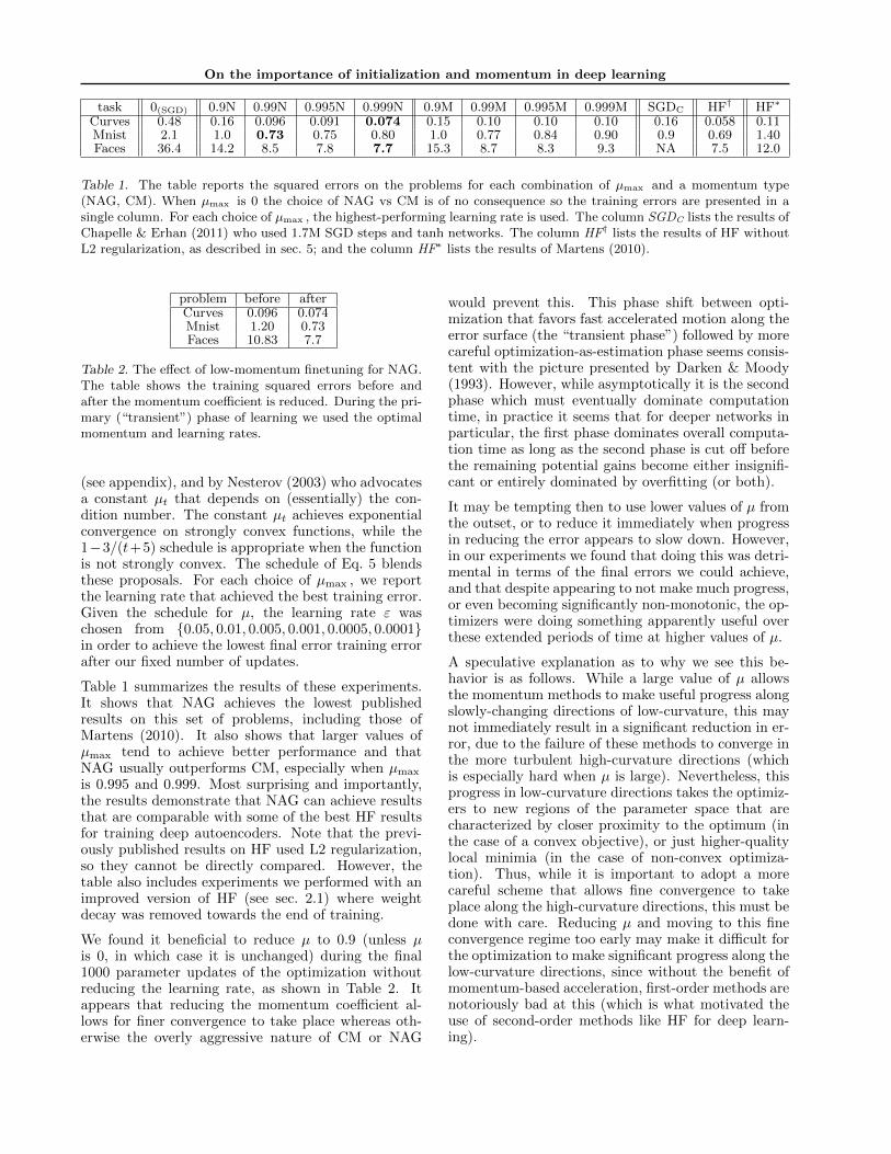
connection type sparsity scalein-to-hid (add,mul) dense 0.001·N(0, 1)

in-to-hid (mem) dense 0.1·N(0, 1)hid-to-hid 15 fan-in spectral radius of 1.1hid-to-out dense 0.1·N(0, 1)hid-bias dense 0out-bias dense average of outputs

Table 4. The RNN initialization used in the experiments.The scale of the vis-hid connections is problem dependent.

Each task involved optimizing the parameters of a ran-domly initialized RNN with 100 standard tanh hiddenunits (the same model used by Martens & Sutskever(2011)). The tasks were designed by Hochreiter &Schmidhuber (1997), and are referred to as training“problems”. See sec. A.3 of the appendix for details.

4.1. ESN-based Initialization

As argued by Jaeger & Haas (2004), the spectral ra-dius of the hidden-to-hidden matrix has a profoundeffect on the dynamics of the RNN’s hidden state(with a tanh nonlinearity). When it is smaller than1, the dynamics will have a tendency to quickly “for-get” whatever input signal they may have been ex-posed to. When it is much larger than 1, the dy-namics become oscillatory and chaotic, allowing it togenerate responses that are varied for different inputhistories. While this allows information to be retainedover many time steps, it can also lead to severe explod-ing gradients that make gradient-based learning muchmore difficult. However, when the spectral radius isonly slightly greater than 1, the dynamics remain os-cillatory and chaotic while the gradient are no longerexploding (and if they do explode, then only “slightlyso”), so learning may be possible with a spectral ra-dius of this order. This suggests that a spectral radiusof around 1.1 may be effective.

To achieve robust results, we also found it is essentialto carefully set the initial scale of the input-to-hiddenconnections. When training RNNs to solve those tasksthat possess many random and irrelevant distractor in-puts, we found that having the scale of these connec-tions set too high at the start led to relevant informa-tion in the hidden state being too easily “overwritten”by the many irrelevant signals, which ultimately ledthe optimizer to converge towards an extremely poorlocal minimum where useful information was never re-layed over long distances. Conversely, we found that ifthis scale was set too low, it led to significantly slowerlearning. Having experimented with multiple scales wefound that a Gaussian draw with a standard deviationof 0.001 achieved a good balance between these con-cerns. However, unlike the value of 1.1 for the spectralradius of the dynamics matrix, which worked well onall tasks, we found that good choices for initial scaleof the input-to-hidden weights depended a lot on theparticular characteristics of the particular task (such


as its dimensionality or the input variance). Indeed,for tasks that do not have many irrelevant inputs, alarger scale of the input-to-hidden weights (namely,0.1) worked better, because the aforementioned dis-advantage of large input-to-hidden weights does notapply. See table 4 for a summary of the initializationsused in the experiments. Finally, we found centering(mean subtraction) of both the inputs and the outputsto be important to reliably solve all of the trainingproblems. See the appendix for more details.

4.2. Experimental Results

We conducted experiments to determine the effi-cacy of our initializations, the effect of momentum,and to compare NAG with CM. Every learning trialused the aforementioned initialization, 50,000 param-eter updates and on minibatches of 100 sequences,and the following schedule for the momentum co-efficient µ: µ = 0.9 for the first 1000 parameter,after which µ = µ0, where µ0 can take the fol-lowing values {0, 0.9, 0.98, 0.995}. For each µ0, weuse the empirically best learning rate chosen from{10−3, 10−4, 10−5, 10−6}.

The results are presented in Table 5, which are the av-erage loss over 4 different random seeds. Instead of re-porting the loss being minimized (which is the squarederror or cross entropy), we use a more interpretablezero-one loss, as is standard practice with these prob-lems. For the bit memorization, we report the frac-tion of timesteps that are computed incorrectly. Andfor the addition and the multiplication problems, wereport the fraction of cases where the RNN the errorin the final output prediction exceeded 0.04.

Our results show that despite the considerable long-range dependencies present in training data for theseproblems, RNNs can be successfully and robustlytrained to solve them, through the use of the initial-ization discussed in sec. 4.1, momentum of the NAGtype, a large µ0, and a particularly small learning rate(as compared with feedforward networks). Our resultsalso suggest that with larger values of µ0 achieve bet-ter results with NAG but not with CM, possibly due toNAG’s tolerance of larger µ0’s (as discussed in sec. 2).

Although we were able to achieve surprisingly goodtraining performance on these problems using a suf-ficiently strong momentum, the results of Martens &Sutskever (2011) appear to be moderately better andmore robust. They achieved lower error rates and theirinitialization was chosen with less care, although theinitializations are in many ways similar to ours. No-tably, Martens & Sutskever (2011) were able to solvethese problems without centering, while we had touse centering to solve the multiplication problem (theother problems are already centered). This suggeststhat the initialization proposed here, together with themethod of Martens & Sutskever (2011), could achieve

even better performance. But the main achievementof these results is a demonstration of the ability ofmomentum methods to cope with long-range tempo-ral dependency training tasks to a level which seemssufficient for most practical purposes. Moreover, ourapproach seems to be more tolerant of smaller mini-batches, and is considerably simpler than the partic-ular version of HF proposed in Martens & Sutskever(2011), which used a specialized update damping tech-nique whose benefits seemed mostly limited to trainingRNNs to solve these kinds of extreme temporal depen-dency problems.

5. Momentum and HF

Truncated Newton methods, that include the HFmethod of Martens (2010) as a particular example,work by optimizing a local quadratic model of theobjective via the linear conjugate gradient algorithm(CG), which is a first-order method. While HF, likeall truncated-Newton methods, takes steps computedusing partially converged calls to CG, it is naturallyaccelerated along at least some directions of lower cur-vature compared to the gradient. It can even be shown(Martens & Sutskever, 2012) that CG will tend to fa-vor convergence to the exact solution to the quadraticsub-problem first along higher curvature directions(with a bias towards those which are more clusteredtogether in their curvature-scalars/eigenvalues).

While CG accumulates information as it iterates whichallows it to be optimal in a much stronger sense thanany other first-order method (like NAG), once it isterminated, this information is lost. Thus, standardtruncated Newton methods can be thought of as per-sisting information which accelerates convergence (ofthe current quadratic) only over the number of itera-tions CG performs. By contrast, momentum methodspersist information that can inform new updates acrossan arbitrary number of iterations.

One key difference between standard truncated New-ton methods and HF is the use of “hot-started” calls toCG, which use as their initial solution the one found atthe previous call to CG. While this solution was com-puted using old gradient and curvature informationfrom a previous point in parameter space and possi-bly a different set of training data, it may be well-converged along certain eigen-directions of the newquadratic, despite being very poorly converged alongothers (perhaps worse than the default initial solution

of ~0). However, to the extent to which the new localquadratic model resembles the old one, and in partic-ular in the more difficult to optimize directions of low-curvature (which will arguably be more likely to per-sist across nearby locations in parameter space), theprevious solution will be a preferable starting point to0, and may even allow for gradually increasing levelsof convergence along certain directions which persist


problem biases 0 0.9N 0.98N 0.995N 0.9M 0.98M 0.995Madd T = 80 0.82 0.39 0.02 0.21 0.00025 0.43 0.62 0.036mul T = 80 0.84 0.48 0.36 0.22 0.0013 0.029 0.025 0.37

mem-5 T = 200 2.5 1.27 1.02 0.96 0.63 1.12 1.09 0.92mem-20 T = 80 8.0 5.37 2.77 0.0144 0.00005 1.75 0.0017 0.053

Table 5. Each column reports the errors (zero-one losses; sec. 4.2) on different problems for each combination of µ0 andmomentum type (NAG, CM), averaged over 4 different random seeds. The “biases” column lists the error attainable bylearning the output biases and ignoring the hidden state. This is the error of an RNN that failed to “establish communi-cation” between its inputs and targets. For each µ0, we used the fixed learning rate that gave the best performance.

in the local quadratic models across many updates.

The connection between HF and momentum methodscan be made more concrete by noticing that a singlestep of CG is effectively a gradient update taken fromthe current point, plus the previous update reapplied,just as with NAG, and that if CG terminated after just1 step, HF becomes equivalent to NAG, except that ituses a special formula based on the curvature matrixfor the learning rate instead of a fixed constant. Themost effective implementations of HF even employ a“decay” constant (Martens & Sutskever, 2012) whichacts analogously to the momentum constant µ. Thus,in this sense, the CG initializations used by HF allowus to view it as a hybrid of NAG and an exact second-order method, with the number of CG iterations usedto compute each update effectively acting as a dialbetween the two extremes.

Inspired by the surprising success of momentum-basedmethods for deep learning problems, we experimentedwith making HF behave even more like NAG than it al-ready does. The resulting approach performed surpris-ingly well (see Table 1). For a more detailed accountof these experiments, see sec. A.6 of the appendix.

If viewed on the basis of each CG step (instead ofeach update to parameters θ), HF can be thought ofas a peculiar type of first-order method which approx-imates the objective as a series of quadratics only sothat it can make use of the powerful first-order CGmethod. So apart from any potential benefit to globalconvergence from its tendency to prefer certain direc-tions of movement in parameter space over others, per-haps the main theoretical benefit to using HF over afirst-order method like NAG is its use of CG, which,while itself a first-order method, is well known to havestrongly optimal convergence properties for quadrat-ics, and can take advantage of clustered eigenvaluesto accelerate convergence (see Martens & Sutskever(2012) for a detailed account of this well-known phe-nomenon). However, it is known that in the worstcase that CG, when run in batch mode, will convergeasymptotically no faster than NAG (also run in batchmode) for certain specially designed quadratics withvery evenly distributed eigenvalues/curvatures. Thusit is worth asking whether the quadratics which ariseduring the optimization of neural networks by HF aresuch that CG has a distinct advantage in optimizing

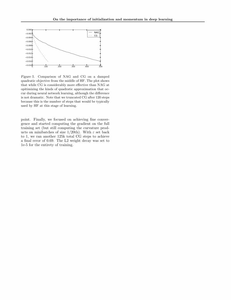
them over NAG, or if they are closer to the aforemen-tioned worst-case examples. To examine this questionwe took a quadratic generated during the middle of atypical run of HF on the curves dataset and comparedthe convergence rate of CG, initialized from zero, toNAG (also initialized from zero). Figure 5 in the ap-pendix presents the results of this experiment. Whilethis experiment indicates some potential advantages toHF, the closeness of the performance of NAG and HFsuggests that these results might be explained by thesolutions leaving the area of trust in the quadratics be-fore any extra speed kicks in, or more subtly, that thefaithfulness of approximation goes down just enoughas CG iterates to offset the benefit of the accelerationit provides.

6. Discussion

Martens (2010) and Martens & Sutskever (2011)demonstrated the effectiveness of the HF method asa tool for performing optimizations for which previ-ous attempts to apply simpler first-order methods hadfailed. While some recent work (Chapelle & Erhan,2011; Glorot & Bengio, 2010) suggested that first-ordermethods can actually achieve some success on thesekinds of problems when used in conjunction with goodinitializations, their results still fell short of those re-ported for HF. In this paper we have completed thispicture and demonstrated conclusively that a largepart of the remaining performance gap that is notaddressed by using a well-designed random initializa-tion is in fact addressed by careful use of momentum-based acceleration (possibly of the Nesterov type). Weshowed that careful attention must be paid to the mo-mentum constant µ, as predicted by the theory forlocal and convex optimization.

Momentum-accelerated SGD, despite being a first-order approach, is capable of accelerating directionsof low-curvature just like an approximate Newtonmethod such as HF. Our experiments support the ideathat this is important, as we observed that the use ofstronger momentum (as determined by µ) had a dra-matic effect on optimization performance, particularlyfor the RNNs. Moreover, we showed that HF can beviewed as a first-order method, and as a generalizationof NAG in particular, and that it already derives someof its benefits through a momentum-like mechanism.


References

Bengio, Y., Simard, P., and Frasconi, P. Learninglong-term dependencies with gradient descent is diffi-cult. IEEE Transactions on Neural Networks, 5:157–166,1994.

Bengio, Y., Lamblin, P, Popovici, D., and Larochelle, H.Greedy layer-wise training of deep networks. In In NIPS.MIT Press, 2007.

Bottou, L. and LeCun, Y. Large scale online learning. InAdvances in Neural Information Processing Systems 16:Proceedings of the 2003 Conference, volume 16, pp. 217.MIT Press, 2004.

Chapelle, O. and Erhan, D. Improved Preconditioner forHessian Free Optimization. In NIPS Workshop on DeepLearning and Unsupervised Feature Learning, 2011.

Cotter, A., Shamir, O., Srebro, N., and Sridharan, K. Bet-ter mini-batch algorithms via accelerated gradient meth-ods. arXiv preprint arXiv:1106.4574, 2011.

Dahl, G.E., Yu, D., Deng, L., and Acero, A. Context-dependent pre-trained deep neural networks for large-vocabulary speech recognition. Audio, Speech, and Lan-guage Processing, IEEE Transactions on, 20(1):30–42,2012.

Darken, C. and Moody, J. Towards faster stochastic gra-dient search. Advances in neural information processingsystems, pp. 1009–1009, 1993.

Glorot, X. and Bengio, Y. Understanding the difficultyof training deep feedforward neural networks. In Pro-ceedings of AISTATS 2010, volume 9, pp. 249–256, may2010.

Graves, A. Sequence transduction with recurrent neuralnetworks. arXiv preprint arXiv:1211.3711, 2012.

Hinton, G and Salakhutdinov, R. Reducing the dimension-ality of data with neural networks. Science, 313:504–507,2006.

Hinton, G., Deng, L., Yu, D., Dahl, G., Mohamed, A.,Jaitly, N., Senior, A., Vanhoucke, V., Nguyen, P.,Sainath, T., et al. Deep neural networks for acousticmodeling in speech recognition. IEEE Signal ProcessingMagazine, 2012.

Hinton, G.E., Osindero, S., and Teh, Y.W. A fast learningalgorithm for deep belief nets. Neural computation, 18(7):1527–1554, 2006.

Hochreiter, S. and Schmidhuber, J. Long short-term mem-ory. Neural computation, 9(8):1735–1780, 1997.

Jaeger, H. personal communication, 2012.

Jaeger, H. and Haas, H. Harnessing nonlinearity: Pre-dicting chaotic systems and saving energy in wirelesscommunication. Science, 304:78–80, 2004.

Krizhevsky, A., Sutskever, I., and Hinton, G. Imagenetclassification with deep convolutional neural networks.In Advances in Neural Information Processing Systems25, pp. 1106–1114, 2012.

Lan, G. An optimal method for stochastic composite op-timization. Mathematical Programming, pp. 1–33, 2010.

LeCun, Y., Bottou, L., Orr, G., and Muller, K. Efficientbackprop. Neural networks: Tricks of the trade, pp. 546–546, 1998.

Martens, J. Deep learning via Hessian-free optimization.In Proceedings of the 27th International Conference onMachine Learning (ICML), 2010.

Martens, J. and Sutskever, I. Learning recurrent neuralnetworks with hessian-free optimization. In Proceedingsof the 28th International Conference on Machine Learn-ing (ICML), pp. 1033–1040, 2011.

Martens, J. and Sutskever, I. Training deep and recurrentnetworks with hessian-free optimization. Neural Net-works: Tricks of the Trade, pp. 479–535, 2012.

Mikolov, Tomas, Sutskever, Ilya, Deoras, Anoop, Le,Hai-Son, Kombrink, Stefan, and Cernocky, J. Sub-word language modeling with neural networks. preprint(http://www. fit. vutbr. cz/imikolov/rnnlm/char. pdf),2012.

Mohamed, A., Dahl, G.E., and Hinton, G. Acoustic mod-eling using deep belief networks. Audio, Speech, andLanguage Processing, IEEE Transactions on, 20(1):14–22, Jan. 2012.

Nesterov, Y. A method of solving a convex program-ming problem with convergence rate O(1/sqr(k)). SovietMathematics Doklady, 27:372–376, 1983.

Nesterov, Y. Introductory lectures on convex optimization:A basic course, volume 87. Springer, 2003.

Orr, G.B. Dynamics and algorithms for stochastic search.1996.

Polyak, B.T. Some methods of speeding up the convergenceof iteration methods. USSR Computational Mathematicsand Mathematical Physics, 4(5):1–17, 1964.

Raiko, Tapani, Valpola, Harri, and LeCun, Yann. Deeplearning made easier by linear transformations in percep-trons. In NIPS 2011 Workshop on Deep Learning andUnsupervised Feature Learning, Sierra Nevada, Spain,2011.

Sutskever, I., Martens, J., and Hinton, G. Generatingtext with recurrent neural networks. In Proceedings ofthe 28th International Conference on Machine Learning,ICML ’11, pp. 1017–1024, June 2011.

Wiegerinck, W., Komoda, A., and Heskes, T. Stochas-tic dynamics of learning with momentum in neural net-works. Journal of Physics A: Mathematical and General,27(13):4425, 1999.


40 30 20 10 0 10 20 3040

30

20

10

0

10

20

30

Figure 2. The trajectories of CM, NAG, and SGD areshown. Although the value of the momentum is identi-cal for both experiments, CM exhibits oscillations alongthe high-curvature directions, while NAG exhibits no suchoscillations. The global minimizer of the objective is at(0,0). The red curve shows gradient descent with the samelearning rate as NAG and CM, the blue curve shows NAG,and the green curve shows CM. See section 2 of the paper.

Appendix

A.1 Derivation of Nesterov’sAccelerated Gradient as a MomentumMethod

Nesterov’s accelerated gradient is an iterative algo-rithm that was originally derived for non-stochasticgradients. It is initialized by setting k = 0, a0 = 1,θ−1 = y0, y0 to an arbitrary parameter setting, zto an arbitrary parameter setting, and ε−1 = ‖y0 −z‖/‖∇f(y0)−∇f(z)‖. It then repeatedly updates itsparameters with the following equations:

εt = 2−iεt−1 (6)

(here i is the smallest positive integer for which

f(yt)− f(yt − 2−iεt−1∇f(yt)) ≥ 2−iεt−1‖∇f(yt)‖2

2)

θt = yt − εt∇f(yt) (7)

at+1 =

(1 +

√4a2t + 1

)/2 (8)

yt+1 = θt + (at − 1)(θt − θt−1)/at+1 (9)

The above presentation is relatively opaque and couldbe difficult to understand, so we will rewrite theseequations in a more intuitive manner.

The learning rate εt is adapted to always be smallerthan the reciprocal of the “observed” Lipshitz coeffi-cient of ∇f around the trajectory of the optimization.Alternatively, if the Lipshitz coefficient of the deriva-tive is known to be equal to L, then setting εt = 1/L

for all t is sufficient to obtain the same theoreticalguarantees. This method for choosing the learningrate assumes that f is not noisy, and will result intoo-large learning rates if the objective is stochastic.

To understand the sequence at, we note that thefunction x →

(1 +√

4x2 + 1)/2 quickly approaches

x → x + 0.5 from below as x → ∞, so at ≈ (t + 4)/2for large t, and thus (at−1)/at+1 (from eq. 9) behaveslike 1− 3/(t+ 5).

Finally, if we define

vt ≡ θt − θt−1 (10)

µt ≡ (at − 1)/at+1 (11)

then the combination of eqs. 9 and 11 implies:

yt = θt−1 + µt−1vt−1

which can be used to rewrite eq. 7 as follows:

θt = θt−1 + µt−1vt−1 − εt−1∇f(θt−1 + µt−1vt−1)(12)

vt = µt−1vt−1 − εt−1∇f(θt−1 + µt−1vt−1) (13)

where eq. 13 is a consequence of eq. 10. Alternatively:

vt = µt−1vt−1 − εt−1∇f(θt−1 + µt−1vt−1) (14)

θt = θt−1 + vt (15)

where µt ≈ 1− 3/(t+ 5). (Nesterov, 1983) shows thatif f is a convex function with an L-Lipshitz contin-uous derivative, then the above method satisfies thefollowing:

f(θt)− f(θ∗) ≤ 4L‖θ−1 − θ∗‖2

(t+ 2)2(16)

To understand the quadratic speedup obtained by themomentum, consider applying momentum to a linearfunction. In this case, the i-th step of the momentummethod will be of distance proportional to i; thereforeN steps could traverse a quadratically longer distance:1 + 2 + · · ·+N = O(N2).

A.2 Details for Theorem 2.1

We will first formulate and prove a result which es-tablishes the well known fact that first-order meth-ods such CM and NAG are invariant to orthonormaltransformations (i.e. rotations) such as U . In partic-ular, we will will show that the sequence of iteratesobtained by applying NAG and CM to the reparam-eterized quadratic p, is given by U times sequence ofiterates obtained by applying NAG and CM to theoriginal quadratic q. Note that the only fact we useabout U at this stage is that it is orthonormal/unitary,not that it diagonalizes q.


Proposition 6.1. Let {(µi, εi)}∞i=1 be an arbitrary se-quence of learning rates, let x0, v0 be an arbitrary ini-tial position and velocity, and let {(xi, vi)}∞i=0 be thesequence of iterates obtained by CM by optimizing qstarting from x0, v0, with the learning parameters µi, εiat iteration i.

Next, let y0, w0 be given by Ux0, Uv0, and let{(yi, wi)}∞i=0 be the sequence of iterates obtained byCM by optimizing p starting from y0, w0, with thelearning parameters µi, εi at iteration i.

Then the following holds for all i:

yi = Uxi

wi = Uvi

The above also applies when CM is replaced with NAG.

Proof. First, notice that

xi+1 = CMx(µi, q, xi, vi)

vi+1 = CMv(µi, q, xi, vi)

and that

yi+1 = CMx(µi, p, yi, wi)

wi+1 = CMv(µi, p, yi, wi)

The proof is by induction. The claim is immediatefor i = 0. To see that it holds for i + 1 assuming i,consider:

wi+1 = wi + ε∇yip(yi)

= wi + εU∇xip(yi) (chain rule using yi = Uxi)

= wi + εU∇xiq(U>yi) (definition of p)

= wi + εU∇xiq(xi) (xi = U>yi)

= Uvi + εU∇xiq(xi) (by induction)

= U(vi + ε∇xiq(xi))

= Uvi+1

Using the above, we get

yi+1 = yi + wi+1

= Uxi + Uvi+1

= Uxi+1

yi+1 = yi + wi+1 = Uxi + Uvi+1 = Uxi+1

This completes the proof for CM; the proof for NAGis nearly identical.

Given this result, and reparameterization p of q ac-cording to its eigencomponents, the results of Theorem2.1 can thus be

Proof of Theorem 2.1. We first show that for separa-ble problems, CM (or NAG) is precisely equivalent tomany simultaneous applications of CM (or NAG) tothe one-dimensional problems that correspond to eachproblem dimension. We then show that for NAG, theeffective momentum for a one-dimensional problem de-pends on its curvature. We prove these results for onestep of CM or NAG, although these results generalizeto larger n.

Consider one step of CMv:

CMv(µ, p, y, v) = µv − ε∇p(y)

= (µ[v]1 − ε∇[y]1p(y), . . . , µ[v]n − ε∇[y]np(y))

= (µ[v]1 − ε∇[p]1([y]1), . . . , µ[v]n − ε∇[p]n([y]n))

= (CMv(µ, [p]1, [y]1, [v]1), . . . , CMv(µ, [p]n, [y]n, [v]n))

This shows that one step of CMv on q is preciselyequivalent to n simultaneous applications of CMv tothe one-dimensional quadratics [q]i, all with the sameµ and ε. A similar argument shows a single step ofeach of CMx, on NAGx, and NAGv can be obtainedby applying each of them to the n one-dimensionalquadratics [q]i.

Next we show that NAG, applied to a one-dimensionalquadratic with a momentum coefficient µ, is equiva-lent to CM applied to the same quadratic and withthe same learning rate, but with a momentum co-efficient µ(1 − ελ). We show this by expandingNAGv(µ, [p]i, y, v) (where y and v are scalars):

NAGv(µ, [q]i, y, v) = µv − ε∇[p]i(y + µv)

= µv − ε(λi(y + µv) + ci)

= µv − ελiµv − ε(λiy + ci)

= µ(1− ελi)v − ε∇[p]i(y)

= CMv(µ(1− ελi), [p]i, v, y)

Since Eq. 2 is identical to 4, it follows that

NAGx(µ, [p]i, y, v) = CMx(µ(1− ελi), [p]i, y, v)

for all i.

A.3. Autoencoder Problem Details

We experiment with the three autoencoder problemsfrom Hinton & Salakhutdinov (2006), which are de-scribed in Table 6.

A.4. RNN Problem Details

We considered 4 of the pathological long term de-pendency “problems” from Hochreiter & Schmidhu-ber (1997), which consist of artificial datasets designedto have various non-trivial long-range dependencies.


0 20 40 60 80

0

20

40

60

80

100

0 20 40 60 80

0

20

40

60

80

100

0 20 40 60 80

0

20

40

60

80

100

Figure 3. In each figure, the vertical axis is time, and the horizontal axis are units. The leftmost figure shows the hiddenstate sequences of an RNN on the addition problem with the aforementioned parameter initialization. Note the “gentle”oscillations of the hidden states. The middle figure shows the hidden state sequence of the same RNN after 1000 parameterupdates. The hidden state sequence is almost indistinguishable, differing by approximately 10−4 for each pixel, so despitethe little progress that has been made, the oscillations are preserved, and thus the parameter setting still have a chance ofsolving the problem. The rightmost figure shows an RNN with the same initialization after 1000 parameter updates, wherethe output biases were initialized to zero. Notice how the hidden state sequence has many fewer oscillations, althoughboth parameter settings fail to establish communication between the inputs and the target.

name dim size architectureCurves 784 20,000 784-400-200-100-50-25-6Mnist 784 60,000 784-1000-500-250-30Faces 625 103,500 625-2000-1000-500-30

Table 6. The networks’ architectures and the sizes of thedatasets.

These were the 5-bit memorization task, the 20-bitmemorization task, the addition problem, and the mul-tiplication problem. These artificial problems wereeach designed to be impossible to learn with regularRNNs using standard optimization methods, owing tothe presence of long-range temporal dependencies ofthe target outputs on the early inputs. And in partic-ular, despite the results of ?, they cannot be learnedwith ESNs that have 100 conventional hidden units(Jaeger, 2012)1.

In the 5-bit memorization problem, the input sequenceconsists of 5 bits that are followed by a large numberof blank symbols. The target sequence consists of thesame 5 bits occurring at the end of the sequence, pre-ceded by blanks. The 20-bit memorization problem issimilar to the 5-bit memorization problem, but the 5-bits are replaced with ten 5-ary symbols, so that eachsequence contains slightly more than 20 bits of infor-

1Small ESNs that use leaky integration can achieve verylow training errors on these problems, but the leaky inte-gration is well-suited for the addition and the multiplica-tion but not the memorization problems.

Figure 4. The memorization and the addition problems.The goal of the memorization problem is to output theinput bits in the correct order. The goal of the additionand the multiplication problem is to output the sum (orthe product) of the two marked inputs.

mation. In the addition problem, the input sequenceconsists of pairs (x, y) of real numbers presented in se-quence, where each x is a drawn from U [0, 1] and eachy is a binary “marker” in {0, 1}. The final entry of thetarget output sequence is determined as the sum ofthe x component for the two pairs whose y componentis 1. The multiplication problem is analogous, and wefollow the precise format used by Martens & Sutskever(2011). To achieve low error on each of these tasks theRNN must learn to memorize and transform some in-formation contained at the beginning of the sequence


within its hidden state, retaining it all of the way to theend. This is made especially difficult because there areno easier-to-learn short or medium-term dependenciesthat can act as hints to help the learning see the long-term ones, and because of the noise in the additionand the multiplication problems.

A.5 The effect of bias centering

In our experiments, we observed that the hidden stateoscillations, which are likely important for relaying in-formation across long distances, had a tendency to dis-appear after the early stages of learning (see fig. 3),causing the optimization to converge to a poor localoptimum. We surmised that this tendency was dueto fact that the smallest modification to the parame-ters (as measured in the standard norm - the quantitywhich steepest descent can be thought of as minimiz-ing) that allowed the output units to predict the av-erage target output, involved making the outputs con-stant by way of making the hidden state constant. Bycentering the target outputs, the initial bias is correctby default, and thus the optimizer is not forced intomaking this “poor early choice” that dooms it lateron.

Similarly, we found it necessary to center the inputsto reliably solve the multiplication problem; the mo-mentum methods were unable to solve this problemwithout input centering. We speculate that the reasonfor this is that the inputs associated with the multipli-cation problem are positive, causing the hidden stateto drift in the direction of the input-to-hidden vector,which in turn leads to saturation of the hidden state.When the inputs are centered, the net input to the hid-den units will initial be closer to zero when averagedover a reasonable window of time, thus preventing thisissue.

Figure 3 shows how the hidden state sequence evolveswhen the output units are not centered. While theoscillations of the RNN’s hidden state are preservedif the output bias is initialized to be the mean of thetargets, they disappear if the output bias is set to zero(in this example, the mean of the targets is 0.5). Thisis a consequence of the isotropic nature of stochasticgradient descent which causes it to minimize the L2

distance of its optimization paths, and of the fact thatthe L2-closest parameter setting that outputs the av-erage of the targets is obtained by slightly adjustingboth the biases and making the hidden states constant,to utilize the hidden-to-output weights.

A.6 Hybrid HF-Momentum approach

Our hybrid HF-momentum algorithm, is characterizedby the following changes to the original approach out-lined by Martens (2010): we disposed of the line search

and used a fixed learning rate of 1 which, after somepoint chosen by hand, we gradually decayed to zero us-ing a simple schedule; we gradually increased the valueof the decay constant (similarly to how we increasedµ); and we used smaller minibatches, while computingthe gradient only on the current minibatch (as opposedto the full dataset - as is commonly done with HF).Analogously to our experiments with momentum, weadjusted the settings near the end of optimization (af-ter the transient phase) to improve fine-grained localconvergence/stochastic estimation. In particular, weswitched back to using a more traditional version ofHF along the lines of the one described by Martens(2010), which involved using much larger minibatches,or just computing the gradient on more data/the entiretraining set, raising the learning rate back to 1 (or ashigh as the larger minibatches permit), etc., and alsodecreasing the L2 weight decay to squeeze out someextra performance.

The results of these experiments were encouraging, al-though preliminary, and we report them in Table 1,noting that they are not directly comparable to theexperiments performed with CM and NAG due to theof use incomparable amounts of computation (feweriterations, but with large minibatches).

For each autoencoder training task we ran we hand-designed a schedule for the learning rate (ε), decayconstant (µ), and minibatch size (s), after a smallamount of trial and error. The details for CURVESand MNIST are given below.

For CURVES, we first ran HF iterations with 50 CGsteps each, for a total of 250k CG steps, using ε = 1.0,µ = 0.95 and with gradient and curvature productscomputed on minibatches consisting of 1/16th of thetraining set. Next, we increased µ to 0.999 and an-nealed ε according to the schedule 500/(t − 4000).The error reach 0.0094 by this point, and from herewe tuned the method to achieve fine local conver-gence, which we achieved primarily through runningthe method in full batch mode. We first ran HF for100k total CG steps with the number of CG steps perupdate increased to 200, µ lowered to 0.995, and εraised back to 1 (which was stable because we wererunning in batch mode) . The error reach 0.087 bythis point. Finally, we lowered the L2 weight decayfrom 2e-5 (which was used in (Martens, 2010)) to nearzero and ran 500k total steps more, to arrive at anerror of 0.058.

For MNIST, we first ran HF iterations with 50 CGsteps each, for a total of 25k CG steps, using ε = 1.0,µ = 0.95 and with gradient and curvature productscomputed on minibatches consisting of 1/20th of thetraining set. Next, we increased µ to 0.995, ε was an-nealed according to 250/t, and the method was run foranother 225k CG steps. The error reach 0.81 by this


0 100 200 300 400 500−0.018

−0.016

−0.014

−0.012

−0.010

−0.008

−0.006

−0.004

−0.002

0.000

NAGCG

Figure 5. Comparison of NAG and CG on a dampedquadratic objective from the middle of HF. The plot showsthat while CG is considerably more effective than NAG atopitimizing the kinds of quadratic approximation that oc-cur during neural network learning, although the differenceis not dramatic. Note that we truncated CG after 120 stepsbecause this is the number of steps that would be typicallyused by HF at this stage of learning.

point. Finally, we focused on achieving fine conver-gence and started computing the gradient on the fulltraining set (but still computing the curvature prod-ucts on minibatches of size 1/20th). With ε set backto 1, we ran another 125k total CG steps to achievea final error of 0.69. The L2 weight decay was set to1e-5 for the entirety of training.

Documents

On the importance of initialization and momentum …hinton/absps/momentum.pdfOn the importance of initialization and momentum in deep learning certain situations. In particular, for