BMeteorol. Z. (Contrib. Atm. Sci.), Vol. 30, No. 3, 271–278 (published online March 26, 2021) Boundary-Layer Meteorology© 2021 The authors

On the importance of a viscous surface layer to describe thelower boundary condition for temperatureGünter Gross∗

Institut für Meteorologie und Klimatologie, Leibniz Universität Hannover, Germany

(Manuscript received January 9, 2021; in revised form February 27, 2021; accepted March 1, 2021)

AbstractA viscous sublayer was introduced into a PBL model in order to specify the lower boundary condition fortemperature. The simulated results have been compared against available observations. However, for such acomparison, some of the variables and parameters that are necessary are not known but can be deduced fromobserved data. In this way, surface temperature and thermal diffusivity of the soil, representative for the four-day period studied here, have been estimated from measured data. An optimized relation for the thickness ofthe viscous sublayer δ was found that includes the diurnal variation of the properties of the air flow. Includingthis approach in the model, simulated temperatures in the ground at different levels as well as temperature inthe atmosphere agree very well with the observations. The applicability for a wider range of wind speeds wasdemonstrated by calculating daily maximum temperatures Tmax. An analysis of long-term observations forthe summer season at different operational weather stations consistently show a distinct maximum of Tmaxfor a 10-m wind between 2–3 m/s, which can be explained by the interaction between the molecular transportof heat within the viscous sublayer of thickness δ and the turbulent heat flux.

Keywords: Boundary layer model, surface temperature, viscous sublayer

1 Introduction

To describe atmospheric processes by a numericalmodel, the lower boundary conditions for the meteoro-logical variables in particular need to be specified. Basedon many research papers on the planetary boundarylayer (PBL), it is well established that the vertical pro-files of the variables follow a logarithmic law. Since thislog-function is not defined at height z = 0, a small lengthscale zo is introduced where the lower boundary condi-tions are defined. The roughness length zo can be esti-mated from surface features (Garratt, 1992) and thisconcept can be applied with great success for momen-tum with the wind speed equal to zero at z = zo. How-ever, temperature at this height is not known; instead,it is usually very close to the ground temperature. In-formation about the surface radiation (or skin) tempera-ture To is available. To may be observed or calculated bya surface energy balance equation. To formulate a lowerboundary condition, Deardorff (1974) gives an expres-sion to relate this surface temperature to the temperatureat height z = zo (see Eq. (2.9)).

The near surface temperature is an essential param-eter to estimate the sensible surface heat flux close tothe ground and therefore the energy transfer from thesurface into the boundary layer. However, using the ra-diation temperature instead of the aerodynamic surfacetemperature at a roughness height (T1) may result in sig-nificant errors in calculating the sensible heat flux. Eval-

∗Corresponding author: Günter Gross, Institut für Meteorologie und Klima-tologie, Leibniz Universität Hannover, Herrenhäuser Str. 2, 30419 Hannover,Germany, e-mail: gross@muk.uni-hannover.de

uating Cabauw data, Beljaars and Holtslag (1991)found temperature differences between To and T1 of upto ±6 K for different thermal stratifications. Such largetemperature gradients occur in a very thin layer with athickness on the order of millimeters adjacent to the sur-face. Inside this viscous sublayer, molecular processesare primarily responsible for heat and moisture transferup to a height where turbulence takes over the transport(Garratt, 1992; Sun et al., 1995). The effects of such aviscous sublayer in general have been incorporated intonumerical models and it was shown that this inclusioncan improve model results through a better representa-tion of the sensible heat flux (Liu et al., 1979; Janjic,1994; Chen et al., 1997).

One approach to describe and to calculate sensibleheat flux in the lower part of the atmosphere is the in-troduction of a thermal roughness length for temper-ature zoT , which differs from the zo for momentum(Mahrt, 1996; Zeng and Dickinson, 1998). A reason-able justification to distinguish between these two dif-ferent roughness lengths derives in particular from thefact that the transfer of heat and momentum from theground into the adjacent air is controlled by differentphysical mechanisms. While form drag determines mo-mentum flux, heat flux is due nearly completely to heatconduction.

Although the idea to use different roughness lengthsfor heat and for momentum is supported by observations(Chen et al., 1997), general guidance on how to esti-mate zoT is not available (Zeng and Dickinson, 1998).

A common finding is that the thermal roughnesslength is usually smaller than the roughness length for

© 2021 The authorsDOI 10.1127/metz/2021/1073 Gebrüder Borntraeger Science Publishers, Stuttgart, www.borntraeger-cramer.com

272 G. Gross: Importance of a viscous surface layer to describe the boundary condition for temperature Meteorol. Z. (Contrib. Atm. Sci.)30, 2021

momentum and a simple approach is to describe zoT asa fixed fraction of zo. Garratt (1992) gives an approxi-mation for the roughness length relation of zoT ≈ zo/10,while Beljaars and Holtslag (1991) reported a muchsmaller value of zoT . However, it is reasonable to assumethat a fixed ratio does not cover the broad range of atmo-spheric situations. As a practical approach, Zilitinke-vich (1995) published a relation for zoT /zo that includesthe properties of the air flow. This relation was appliedby Chen et al. (1997), and in comparisons with observa-tions, they found better results for the surface heat fluxand radiation temperature simulations.

As an alternative approach, Janjic (1994, 2019) in-troduced the thickness of the viscous sublayer δ into aweather prediction model to define a lower boundarycondition for temperature for the turbulent atmosphereabove. This value, T1, is expressed as a weighted meanof temperatures at the surface and the lower atmosphere,observed or modelled. The idea of using δ has earlierbeen used by Liu et al. (1979) to estimate the air-sea ex-change of heat.

In this paper, it is shown that the concept of a viscoussublayer, introduced into a high resolution PBL model,is an important link between the surface and the atmo-sphere close to the ground, and in particular, it is im-portant to formulate the lower boundary condition fortemperature by taking into account the thickness δ.

2 Theoretical aspects

2.1 Heat energy budget and viscous sublayer

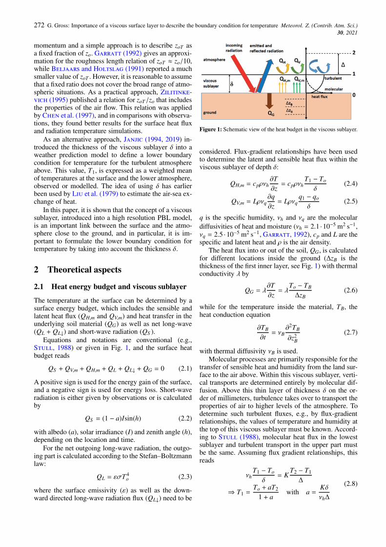
The temperature at the surface can be determined by asurface energy budget, which includes the sensible andlatent heat flux (QH,m and QV,m) and heat transfer in theunderlying soil material (QG) as well as net long-wave(QL + QL↓) and short-wave radiation (QS ).

Equations and notations are conventional (e.g.,Stull, 1988) or given in Fig. 1, and the surface heatbudget reads

QS + QV,m + QH,m + QL + QL↓ + QG = 0 (2.1)

A positive sign is used for the energy gain of the surface,and a negative sign is used for energy loss. Short-waveradiation is either given by observations or is calculatedby

QS = (1 − a)Isin(h) (2.2)

with albedo (a), solar irradiance (I) and zenith angle (h),depending on the location and time.

For the net outgoing long-wave radiation, the outgo-ing part is calculated according to the Stefan–Boltzmannlaw:

QL = εσT 4o (2.3)

where the surface emissivity (ε) as well as the down-ward directed long-wave radiation flux (QL↓) need to be

Figure 1: Schematic view of the heat budget in the viscous sublayer.

considered. Flux-gradient relationships have been usedto determine the latent and sensible heat flux within theviscous sublayer of depth δ:

QH,m = cpρνh∂T∂z

= cpρνhT1 − To

δ(2.4)

QV,m = Lρνq∂q∂z

= Lρνqq1 − qo

δ(2.5)

q is the specific humidity, νh and νq are the moleculardiffusivities of heat and moisture (νh = 2.1 ·10−5 m2 s−1,νq = 2.5 ·10−5 m2 s−1, Garratt, 1992), cp and L are thespecific and latent heat and ρ is the air density.

The heat flux into or out of the soil, QG, is calculatedfor different locations inside the ground (ΔzB is thethickness of the first inner layer, see Fig. 1) with thermalconductivity λ by

QG = λ∂T∂z

= λTo − TB

ΔzB(2.6)

while for the temperature inside the material, TB, theheat conduction equation

∂TB

∂t= νB

∂2TB

∂z2B

(2.7)

with thermal diffusivity νB is used.Molecular processes are primarily responsible for the

transfer of sensible heat and humidity from the land sur-face to the air above. Within this viscous sublayer, verti-cal transports are determined entirely by molecular dif-fusion. Above this thin layer of thickness δ on the or-der of millimeters, turbulence takes over to transport theproperties of air to higher levels of the atmosphere. Todetermine such turbulent fluxes, e.g., by flux-gradientrelationships, the values of temperature and humidity atthe top of this viscous sublayer must be known. Accord-ing to Stull (1988), molecular heat flux in the lowestsublayer and turbulent transport in the upper part mustbe the same. Assuming flux gradient relationships, thisreads

νhT1 − To

δ= K

T2 − T1

Δ

⇒ T1 =To + aT2

1 + awith a =

KδνhΔ

(2.8)

Meteorol. Z. (Contrib. Atm. Sci.)30, 2021

G. Gross: Importance of a viscous surface layer to describe the boundary condition for temperature 273

Table 1: Selected values of the parameter A from literature.

Author assumptions A

Schlichting and Gersten (1997) 5Garratt (1992) A = 5–30Chriss and Caldwell (1984) A = 9–25Gross see below A = 19.2Janjic (1994) M = 10, zo = 0.01 m, u∗ = 0.1 m/s A = 10

M = 30, zo = 0.03 m, u∗ = 0.3 m/s A = 51Deardorff (1974) zo = 0.01 m, u∗ = 0.1 m/s A = 0.8

zo = 0.03 m, u∗ = 0.3 m/s A = 2.1

with eddy diffusivity K and Δ is the thickness of the firstlayer in the atmosphere (see Fig. 1).

The lower boundary condition for temperature in theturbulent layer, T1, is expressed as a weighted meanof the values at the surface (To) and the observationlevel or the lowest level of a model (T2). A similartype of equation can be derived when the estimates ofDeardorff (1974) or Pielke (2002) are used.

T1 = To − 0.74w′ϑ′

κu∗0.13(u∗zo

ν

)0.45

T1 = To + 0.0481(u∗zo

ν

)0.45(T2 − T1)

⇒ T1 =To + bT2

1 + bwith b = 0.0481

(u∗zo

ν

)0.45

(2.9)

In the equation above with Karman constant κ = 0.4,ν is kinematic viscosity (ν = 1.5 · 10−5 m2s−1), rough-ness length zo and friction velocity u∗, the temperatureflux w′ϑ′ is approximated by a flux-gradient relationshipwith K = u∗κΔ/2. For humidity, the same procedure isadopted by replacing temperature with specific humid-ity. It should be noted that T1 from Equation (2.8) is thetemperature at the top of the viscous sublayer at z = δ,while the Deardorff relation results in a temperature atheight z = zo.

The thickness of the viscous sublayer δ determineshow effective and how fast the information is transferredfrom the surface to the turbulent part of the atmosphere.According to Schlichting and Gersten (1997), thedepth of the viscous sublayer is given by

δ = Aν

u∗(2.10)

with a large range of numerical values for A found in theliterature (Table 1).

The parameter A for the Deardorff relation given inTable 1 was obtained by Equations (2.8)–(2.10):

a = b ⇒KδνhΔ

= 0.0481(u∗zo

ν

)0.45

⇒ δ =0.0481κ

(u∗zo

ν

)0.45 νh

u∗

(2.11)

The effects of this wide scatter of the parameter A to es-timate the temperature at the top of the viscous layer, T1,will be studied by using a boundary layer model andcomparing the results against observations.

2.2 The boundary layer model

The studies presented here are restricted to an ideal-ized homogeneous flat terrain and it is justifiable touse a simple PBL model to calculate the distribution ofmeteorological variables in time and height. The PBLmodel consists of prognostic equations for horizontalwind components, temperature including longwave radi-ation fluxes, humidity and turbulence kinetic energy. Allturbulent fluxes are parameterized using K-theory. For amore detailed explanation, see Gross (2012, 2019).

At the upper boundary at a height of 3,000 m, anundisturbed situation is assumed, with prescribed val-ues of 5 m/s for wind, 303 K for potential temperature,0.006 kg/kg for specific humidity and zero turbulencekinetic energy. At the lower boundary at the height ofthe viscous sublayer, the wind is zero, the turbulence ki-netic energy is proportional to the local friction velocitysquared, temperature is determined by a surface energybudget and the specific humidity is according to Gross(1993).

Within the ground, temperature and soil water arecalculated at different levels at depths of 2, 5, 10, 20, 50and 100 cm as described by Maronga et al. (2020). Inthe atmosphere, a grid interval of 2 m up to 10 m heightand an expanded grid above up to 3,000 m is used.

3 Results

To verify the results of this study, additional informa-tion, such as the surface temperature To and the thermaldiffusivity νB of the soil, need to be derived from obser-vations in a first step, followed by a sensitivity study onthe effect of parameter A on obtaining the depth of theviscous surface layer. A final application and compari-son demonstrate the great importance of δ on the dailymaximum temperature, depending on the wind speed.

274 G. Gross: Importance of a viscous surface layer to describe the boundary condition for temperature Meteorol. Z. (Contrib. Atm. Sci.)30, 2021

Figure 2: Observations at the DWD station Braunschweig. Selectedfour-day period is highlighted by the dotted box.

3.1 Observations

Observations at the synoptic station Braunschweig (sta-tion ID 662) of the German Meteorological Service(DWD, 2020) are used for further studies and compar-isons. This station has been selected because a widerange of parameters are available, which are neces-sary if the heat budget of the surface (Eq. (2.1)) isintended to be used. Besides 2-m temperature and10-m wind, global radiation and atmospheric longwaveradiation, soil temperatures as well as soil moisture(Böske, 2020) at different levels (5 cm, 10 cm, 20 cm,50 cm and 100 cm) within the ground are available onan hourly basis. A four-day period, 5–9 August 2020,has been selected for this study (Fig. 2). During thistime, an undisturbed incoming radiation heats up theground and maximum 2-m temperatures increase con-tinuously from 27 °C to 34 °C. In general, the windspeed is low, with higher values around 3 m/s during theday and lower nighttime values (≈ 1 m/s). Observed tem-peratures in the ground are given in Fig. 3. On 8 August,the soil temperature at 5 cm depth is above 39 °C.

3.2 Surface temperature

Besides the calculation of the temperature at the sur-face (To) with a surface energy budget, selected observa-tions in combination with the heat conduction equation(Eq. (2.7)) can be used as an alternative approach. If ob-served temperatures within the soil at various depths are

Figure 3: Observed and simulated soil temperatures at differentdepths.

available, then the discretized Equation (2.7) for the firstlevel in the ground reads (Liebethal and Foken, 2007)

T t+Δt5 cm − T t

5 cm

Δt= νB

T to − 2 T t

5 cm + T t10 cm

Δz2B

→ T to = 2 T t

5 cm − T t10 cm +

T t+Δt5 cm − T t

5 cm

Δt

Δz2B

νB

(3.1)

where ΔzB is the distance of the observations within thesoil (here, 5 cm), Δt is a time step and νB is the ther-mal diffusivity. However, νB is not known for this spe-cific period, but it may also be determined with the dis-cretized heat conduction equation when using observedsoil temperatures at three different depths and rearrang-ing Equation (3.1). For every hour of the period, νB wascalculated in this way and these values are used to deter-mine a 24-hour mean. However, in order to restrict thecalculated values within a realistic range, only thermaldiffusivities 0.04 · 10−6 < νB < 4 · 10−6 m2/s are consid-ered (Table 2).

The larger values of νB in deeper layers are causedby the composition of the soil and different soil mois-ture levels. The last rain before the period consideredhere was on 2 August. While the moisture content of theupper layer was strongly reduced day by day by evapo-transpiration, the deeper part of the soil remains nearlyunchanged, with values of around 10 % by volume.

For simplification and for practical use, a represen-tative value of νB for the four-day period was calcu-lated as a weighted mean for layers 1 and 2, resultingin νB = 0.62 · 10−6 m2/s. This value is on the orderof realistic values known from literature (Hillel, 1998,Zmarsly et al., 2002).

Using this representative value of νB in Equa-tion (3.1), the surface temperature To is calculated witha time step of Δt = 60 s. Finally, the success of the pre-sented approach will be tested by solving the heat con-duction equation with the prescribed To (calculated as

Meteorol. Z. (Contrib. Atm. Sci.)30, 2021

G. Gross: Importance of a viscous surface layer to describe the boundary condition for temperature 275

Table 2: Calculated daily mean of νB (10−6 m2/s) for different soil layers. Number of values to estimate the daily mean are given in brackets.

layers depths used August 5 August 6 August 7 August 8 4-day mean

1 5-10-20 cm 0.33 (21) 0.34 (21) 0.34 (21) 0.35 (20) 0.342 10-20-50 cm 0.70 (22) 0.71 (21) 0.76 (21) 0.71 (20) 0.723 20-50-100 cm 0.79 (20) 0.93 (18) 0.96 (19) 1.04 (17) 0.93

described above) and T−100 cm (observed). The simulatedtemperature distribution within the soil layer at differentlevels is presented in Fig. 3. The calculated diurnal tem-perature variation in all depths is close to the observedvariation, with mean absolute errors for the four-day pe-riod of 0.26 K (5 cm), 0.60 K (10 cm), 0.64 K (20 cm)and 0.24 K (50 cm). Based on these encouraging resultsit can be assumed that, in particular, the estimated sur-face temperature To is in a realistic and credible range.

3.3 Temperature at the top of the viscoussublayer

With the surface temperature To, estimated as describedabove, and the observed 2-m temperature T2, Equa-tion (2.8) can be used to calculate the temperature at thetop of the viscous sublayer T1 for different values of Afrom Table 1. For the Deardorff relation, zo = 0.03 m isused and the friction velocity u∗ is determined from thelogarithmic wind profile with the observed 10-m wind.In order to avoid dividing by zero when calculating δ,a minimum friction velocity of u∗ = 0.01 m/s is used.Results are presented in Fig. 4 for the four-day periodconsidered in this study. Although the diurnal variationis very similar for all calculations, T1 during the day-time becomes lower for larger values of A. An increas-ing value of A means an increasing depth of the viscoussublayer, where molecular transport is of particular im-portance for the transport of heat and moisture. Conse-quently, for larger values of δ, the temperature gradientclose to the ground becomes larger. The effects of Aon T1 are demonstrated by calculating the temperaturedifferences from a reference, for which the result forA = 19.2 is adopted. For values of A smaller than 5, day-time maximum temperatures are around 4 K higher thanfor the reference case. For increasing values of A aboveA = 10, the differences become significantly smaller.The results for the Deardorff relation with a small A(Dd = 0.0481) can be improved by dropping the factorof 0.74 in Equation (2.9) (Dd = 0.065) as suggested byZeng and Dickinson (1998), but this still results inmaximum temperature differences of about 3 K. Duringthe night, the results are very similar because the fric-tion velocity is small, resulting in a larger depth of theviscous sublayer in general.

As described by Foken (2002) the depth of the vis-cous sublayer consists of a laminar layer and a bufferzone above. In this paper, no distinction is made betweenthese two different internal layers. This might explainthe larger values of A to achieve more realistic resultscompared to smaller values (e.g. A = 5, Schlichtingand Gersten, 1997).

Figure 4: Calculated temperatures T1 for different values of A(above) and temperature difference to the results of a reference runwith A = 19.2 (below).

3.4 Soil-atmosphere simulation

In order to stay close to the observations, the PBL modelintroduced above is used to simulate the four-day periodwith specified hourly values of observed global radia-tion and downward longwave radiation. Between thesehourly values, a linear interpolation is used. In order tofind a suitable value for A to estimate the depth of theviscous sublayer and to calculate an appropriate lowerboundary condition for temperature and humidity, nu-merous numerical simulations have been performed fordifferent values of A. The range of parameter A was be-tween 1 and 30 with an increment of 0.1. As a measure toevaluate the results and to quantify the errors, the meanabsolute error between the observed and simulated 2-mtemperatures as well as for soil temperatures at 5 cm inthe ground have been calculated. The results given inFig. 5 show a distinct minimum for both values, withthe smallest error for a value of A around 19.2.

The simulated results with the coupled soil-atmo-sphere PBL model using a viscous sublayer depth ofδ = 19.2ν/u∗ are presented in Fig. 6. Within the ground,temperatures at all depths follow the observations rea-sonably well. Only for the first and the last day ofthe four-day period does the simulated surface tempera-ture To differ shortly after noon from the observed valueby 2–4 K. These differences propagate into the soil, re-sulting in a warmer upper soil layer during the first dayand a slightly cooler layer around the end of the simu-lation period. However, this mismatch has only a smallimpact on the 2-m temperature in the atmosphere. Whilesimulated temperatures on the fourth day follow nearlyperfectly the diurnal course of the observations, larger

276 G. Gross: Importance of a viscous surface layer to describe the boundary condition for temperature Meteorol. Z. (Contrib. Atm. Sci.)30, 2021

Figure 5: Mean absolute error between observed and simulated 2-mtemperatures and for soil temperatures at 5 cm in the ground fordifferent values of the parameter A.

Figure 6: Diurnal variation of simulated temperatures in the lowestatmosphere (above), within the soil (middle) and for δ and κB−1

(below).

daytime differences around noon are obvious for theother days.

A diurnal variation of the thickness of the viscoussublayer is obvious from this figure. During the day,δ is eroded from above by enhanced turbulence, whileovernight, a sublayer depth of around 2 mm is simulated.δ is the height, where the lower boundary conditionfor temperature is defined and therefore comparable tothe thermal roughness length zoT . For a comparison ofthe available observations with regard to zo and zoT , aquantity B−1 is introduced with

κB−1 = lnzo

zoT. (3.2)

Garratt and Hicks (1973) summarized the findingsconcerning B−1 depending on the roughness Reynoldsnumber Re∗ = u∗zo/ν. For the range 10 < Re∗ < 200,they evaluated a typical value of κB−1 ≈ 2. For themeteorological situation adopted here, Re∗ is between50 and 150 and the calculated values 1.5 < κB−1 < 2.3are very comparable to the values given in Garratt andHicks (1973), Kanda et al. (2007) and Li et al. (2017).

3.5 Effects of near surface wind on dailymaximum temperatures

Nighttime minimum temperatures are not very sensitiveto a specific value of the parameter A in Equation (2.9)because a small value of the friction velocity, which istypical for the night, is sufficient to cause a larger depthof the viscous sublayer. However, during the daytimehours with an unstable stratification near the ground, thefriction velocity is large and small differences in u∗ mayresult in significant variations in T1, the lower boundarycondition for atmospheric temperature. In order to findout whether the relation δ = 19.2ν/u∗ is also valid fora wider range of near surface winds, a sensitivity studywas conducted to find a relationship between wind speedand daily maximum 2-m temperature Tmax. For this nu-merical experiment, all parameters were fixed except thesuperimposed wind speed. The meteorological situationrepresents a clear summer day with strong solar radi-ation and therefore simulated maximum temperaturesare, in general, above 30 °C (Fig. 7). The most obviousfeature is a maximum of Tmax for a 10-m wind aroundu = 2.5 m/s. For smaller values of u as well as for largervalues, the maximum temperature at the 2-m level is sig-nificantly lower. This result is compared to observationsat four DWD-stations in the northern part of Germanyalong a west-east running line from Meppen in the westto Lindenberg in the east (DWD, 2020). At these sta-tions, daily maximum temperatures during the summermonths JJA for the period 1990–2019 are evaluated to-gether with the associated wind. The 99-percentile valuefor each wind speed class of 0.5 m/s was adopted as themaximum temperature and plotted in Fig. 7. For all ob-servations of the four selected stations, there also existsa maximum of Tmax for a wind speed around 2–3 m/s.

Meteorol. Z. (Contrib. Atm. Sci.)30, 2021

G. Gross: Importance of a viscous surface layer to describe the boundary condition for temperature 277

Figure 7: Top: Depth of the viscous sublayer δ and turbulent heatflux QH for different wind speeds for the time when Tmax is sim-ulated. Bottom: Daily maximum temperatures depending on windspeed. Observations: thin lines – original data, thick lines – runningmean.

For a better visual comparison, a constant value of 2 K isadded to the simulated temperatures presented in Fig. 7.

This specific relation between daily maximum tem-perature and wind speed can be explained by the twodifferent processes that are responsible for transportingthe surface heat up to the 2-m observation level. At thetime when Tmax is simulated and for low wind condi-tions, δ is relatively large and molecular transport is notvery efficient, resulting in a large temperature gradientwithin the viscous sublayer, with high values of To andsmall values of T1 at the lower boundary of the turbulentlayer (Fig. 7 top). For increasing wind speed, the turbu-lent sensible heat flux QH becomes dominant, resultingin an effective transport of heat into the higher levelsof the atmospheric boundary layer. This turbulent mix-ing of near surface warm air with a larger volume of airabove then prevents higher values of Tmax. Simulationswith a constant value of δ = 1 mm, which correspondsroughly to zo/zoT ≈ 10, cannot reproduce the observa-tions with the same quality. Especially for a smaller fric-tion velocity, larger values of Tmax are calculated withthe assumption δ = const.

4 Conclusions

A one-dimensional boundary layer model was used tostudy the effects and the importance of the viscoussurface layer, especially on the temperature near the

ground. While at the lower boundary the condition forwind can be well specified at a roughness height, thisheight is not appropriate for temperature as well. A rea-sonable explanation for this fact is caused by the differ-ent physical mechanisms for heat and momentum trans-fer very close to the ground. While the heat flux ismainly controlled by heat conduction, the form drag de-termines the momentum flux.

Questions remain on whether an appropriate lowerboundary condition for temperature in the turbulentboundary layer can be determined using available in-formation, such as surface radiation temperature, andthe observed or simulated data, e.g., at 2 m height inthe atmosphere. Usually, the required temperature is ex-pressed as a weighted mean of these two values. Oneweighting factor is the depth of the viscous surfacelayer δ, which determines the effectiveness of molecu-lar heat transfer from the ground up to the height whereturbulence takes over the heat flux into the atmosphere.

It is known that δ depends on friction velocity, molec-ular thermal diffusivity and an empirical factor for whicha wider range of values are published in the literature.In this paper, an optimized empirical factor A is calcu-lated in such a way that temperatures in the atmosphereas well as in the ground can be reproduced with highaccuracy. It is also demonstrated that the variables andparameters that are necessary for such an estimation canbe deduced from observations as well.

The results of a numerical simulation for a four-day period with an optimized A show very good agree-ment with the observed temperatures at 2 m height inthe atmosphere as well as at different depths inside theground. This is largely due to the calculation of a realis-tic surface temperature, which in turn depends on the di-urnal variation of the depths of the viscous surface layer.During the night, δ is on the order of 2 mm, while a day-time value of around 1 mm is calculated.

The great importance of the viscous sublayer depths,depending on the time of the day, becomes particularlyapparent in a final test, where the daily maximum tem-perature Tmax is calculated for different wind speeds.Long term observations at various DWD stations showa pronounced maximum of Tmax for an observed 10-mwind between 2–3 m/s, with a strong decrease for alower wind speed and a weaker decrease towards largervalues. This correlation of Tmax and wind speed, andtherefore friction velocity u∗, can be directly attributedto the thickness of the viscous sublayer. For low valuesof u∗ the thickness is large and heat transfer by molecu-lar diffusion from the ground up to a height where turbu-lence is effective is small. Consequently, the 2-m max-imum temperature benefits to a lesser degree from thehigh surface temperature. For increasing friction veloc-ity, δ decreases and the turbulent sensible heat flux be-comes very efficient at transporting warm air from theground into the atmosphere. This process reduces thesurface temperature and, due to an effective mixing withthe air in the PBL, also reduces Tmax. With a constantvalue of δ, which can be compared to a thermal rough-

278 G. Gross: Importance of a viscous surface layer to describe the boundary condition for temperature Meteorol. Z. (Contrib. Atm. Sci.)30, 2021

ness length, the observations with regard to Tmax cannotbe reproduced with a similar quality.

Based on the results presented in this paper the au-thor recommends to consider a time-dependent viscoussurface layer of variable depth in high resolution PBLmodels (e.g. PALM-4U, Maronga et al., 2020) for a so-phisticated formulation of especially the lower boundarycondition for temperature.

Acknowledgements

The publication of this article was funded by the OpenAccess Fund of Leibniz University Hannover.

References

Beljaars, A.C.M., A.A.M. Holtslag, 1991: Flux parameteri-zation over land surfaces for atmospheric models. – J. Appl.Meteor. 30, 327–341.

Böske, L., 2020: personal communication. – DWD Braun-schweig.

Chen, F., Z. Janjic, K. Mitchell, 1997: Impact of atmo-spheric surface-layer parameterizations in the new land-surface scheme of the NCEP mesoscale eta model. – Bound.-Layer Meteor. 85, 391–421.

Chriss, T.M., D.R. Caldwell, 1984: Universal similarity andthe thickness of the viscous sublayer at the ocean floor. –J. Geophys. Res. 89, 6403–6414.

Deardorff, J.W., 1974: Three-dimensional numerical study ofthe height and mean structure of a heated planetary boundarylayer. – Bound.-Layer Meteor. 7, 81–106.

DWD, 2020: open data. – https://opendata.dwd.de/climate_environment/CDC/observations_germany/climate/hourly/solar/

Foken, Th., 2002: Some aspects of the viscous sublayer – Me-teorol. Z. 11, 267–272.

Garratt, J.R., 1992: The atmospheric boundary layer. – Cam-bridge University Press, 316 pp.

Garratt, J.R., B.B. Hicks, 1973: Momentum, heat and watervapour transfer to and from natural and artificial surfaces. –Quart. J. Roy. Meteor. Soc. 99, 680–687.

Gross, G., 1993: Numerical simulation of canopy flows. –Springer Verlag Berlin, 167 pp.

Gross, G., 2012: Numerical simulation of greening effects foridealised roofs with regional climate forcing. – Meteorol. Z.21, 173–181.

Gross, G., 2019: On the self-ventilation of an urban heat island. –Meteorol. Z. 28, 87–92.

Hillel, D., 1998: Environmental soil physics. – AcademicPress, New York, 771 pp.

Janjic, Z.I., 1994: The step-mountain eta coordinate model:Further developments of the convection, viscous sublayer, andturbulence closure scheme. – Mon. Wea. Rev. 122, 927–945.

Janjic, Z.I., 2019: The surface layer parameterization in theNMM models. – Office note 497, DOI:10.25923/9qej-k604,NOAA Maryland.

Kanda, M., M. Kanega, T. Kawai, R. Moriwaki, H. Sug-awara, 2007: Roughness lengths for momentum and heat de-rived from outdoor urban scale models. J. Appl. Meteor. Cli-matol. 46, 1067–1079.

Li, D., A. Rigden, G. Salvucci, H. Liu, 2017: Reconciling theReynolds number dependence of scalar roughness length andlaminar resistance. – Geophys. Res. Lett. 44, 3193–3200.

Liebethal, C., Th. Foken, 2007: Evaluation of six parameter-ization approaches for the ground heat flux. – Theor. Appl.Climatol. 88, 43–56.

Liu, W.T., K.B. Katsaros, J.A. Businger, 1979: Bulk parame-terization of air-sea exchange of heat and water vapor includ-ing the molecular constraints at the interface. – J. Atmos. Sci.36, 1722–1735.

Mahrt, L., 1996: The bulk aerodynamic formulation over het-erogeneous surfaces. – Bound.-Layer Meteor. 78, 87–119.

Maronga, B., S. Banzhaf, C. Burmeister, T. Esch,R. Forkel, D. Fröhlich, V. Fuka, K.F. Gehrke, J. Geletic,S. Giersch, T. Gronemeier, G. Gross, W. Heldens,A. Hellsten, F. Hoffmann, A. Inagaki, E. Kadasch,F. Kanani-Sühring, K. Ketelsen, B.A. Khan, C. Knigge,H. Knoop, P. Krc, M. Kurppa, H. Maamari, A. Matzer-akis, M. Mauder, M. Pallasch, D. Pavlik, J. Pfafferott,J. Resler, S. Rissmann, E. Russo, M. Salim, M. Schrempf,J. Schwenkel, G. Seckmeyer, S. Schubert, M. Sühring,R. von Tils, L. Vollmer, S. Ward, B. Witha, H. Wurps,J. Zeidler, S. Raasch, 2020: Overview of the PALM modelsystem 6.0. – Geosci. Model Dev. 13, 1335–1372.

Pielke, R.A., 2002: Mesoscale meteorological modeling. – Aca-demic Press, San Diego, 676 pp.

Schlichting, H., K. Gersten, 1997: Grenzschicht-Theorie. –Springer Verlag Berlin, 851 pp.

Stull, R.B., 1988: An introduction to boundary layer meteorol-ogy. Kluwer Academic, 666 pp.

Sun, J., S.K. Esbensen, L. Mahrt, 1995: Estimation of surfaceheat flux. – J. Atmos. Sci. 52, 3162–3171.

Zeng, X., R.E. Dickinson, 1998: Effect of surface sublayer onsurface skin temperature and fluxes. – J. Climate. 11, 537–550.

Zilitinkevich, S.S., 1995: Non-local turbulent transport: Pol-lution dispersion of coherent structure of convective flows. –In: H. Power, N. Moussiopoulos, C.A. Brebbia (Eds.): Airpollution III – Volume I. Air pollution theory and simula-tion. – Computational Mechanics Publications, Southampton,Boston, 53–60.

Zmarsly, E., W. Kuttler, H. Pethe, 2002: Meteorologisch-klimatologisches Grundwissen. – Ulmer Verlag, 176 pp.