Embed Size (px)
Citation preview
SCHOOL OF ECONOMICS AND FINANCE
Discussion Paper 2013-11
On the Impact of the Global Financial Crisis on the Euro Area
Xiaoli He, Jan P.A.M. Jacobs, Gerard H. Kuper and Jenny E. Ligthart
ISSN 1443-8593 ISBN 978-1-86295-919-4
On the Impact of the Global Financial Crisison the Euro Area
Xiaoli HeUniversity of Groningen
Jan P.A.M. Jacobs1
University of Groningen, UTAS, CAMA and CIRANO
Gerard H. KuperUniversity of Groningen
Jenny E. Ligthart2
Tilburg University, University of Groningen, CAMA and CESifo
September 2013
1Send correspondence to: J.P.A.M. Jacobs, Faculty of Economics and Business, University ofGroningen, P.O. Box 800, 9700 AV Groningen, [email protected]
2A few days after this paper was presented at the Workshop on Business Fluctuations andInternational Transmission of Shocks, Kobe University, Kobe, Japan, November 2012, our col-league, co-author and dear friend Jenny Ligthart passed away. This paper could never have beenwritten without her, and the final result would definitely have been better with her input. Wethank Adrian Pagan and participants of the Workshop, in particular Tsutomu Miyagawa, forhelpful comments.
Abstract
This paper analyses the impact of the Global Financial Crisis on the Euro area utilizing asimple dynamic macroeconomic model with interaction between monetary policy and fiscalpolicy. The model consists of an IS curve, a Phillips curve, a term structure relation, a debtaccumulation equation and a Taylor monetary policy rule supplemented with a Zero LowerBound, and a fiscal policy rule. The model is calibrated/estimated for EU-16 countriesfor the period 1980Q1–2009Q4. The impact of the Global Financial Crisis is studied bymeans of impulse responses following a combined, prolonged aggregate demand and publicdebt shock. The simulation mimicking the GFC turns out to work fairly well. However,the required size of the shock is quite large.
Keywords: Global Financial Crisis, euro area, monetary policy, fiscal policy, New Neoclas-sical Synthesis model, Zero Lower Bound
JEL-code: C51, C52, E63
1 Introduction
The Global Financial Crisis (GFC) in 2007–2008 has had an huge impact on the euro area,
and until now the recovery is still not under way. Even worse, the European sovereign debt
crisis triggered by the GFC resulted in large difficulties for several Euro area countries to
refinance their government debt. Starting in late 2009, the Greek government began having
problems to meet its debt obligations, and in April 2010 Greece government bonds were
downgraded to the status of junk bonds, which led to panic in European and even global
financial markets. Despite the fact euro area member states and the IMF provided one
hundred and ten billion euro bail-out loans to Greece in May 2010, the debt crisis did not
stop and even spread to other euro area countries such as Ireland, Portugal and Spain.
Since the Maastricht Treaty was signed by the member countries of the European Union
(EU), individual euro area countries design independent macroeconomic (fiscal) policies.
This makes dealing with the current economic condition in the Euro area quite complicated.
This paper focuses on the impact of the Global Financial Crisis on the euro area. We
utilize a simple dynamic macroeconomic model, which is heavily inspired by Kirsanova,
Stehn and Vines (2005; henceforth KSV), who focus on the interaction between monetary
and fiscal policy of a single economy against shocks in a dynamic setting. They set up a five-
equation model consisting of a dynamic and linearized IS equation with Blanchard-Yaari
consumers (Yaari, 1965; Blanchard, 1985), a Phillips curve (Bean, 1998), a linearized debt
accumulation equation and two policy rules, a Taylor-like monetary policy rule (Taylor,
1995) and a fiscal policy rule. Both monetary and fiscal policy makers are benevolent;
monetary policy makers will make monetary policy do nearly all of the stabilization.
One of the features of the model is the interaction of monetary and fiscal policy. Al-
most all existing models concerning the interaction between monetary and fiscal policy
only include the short-term interest rate and basic macro-founded household consumption
1
structure. However, the long-term interest rate is the relevant interest rate for financing
government debt, and microeconomic elements such as real estate values, stock returns
and living expectation can also considerably influence household consumption behaviour.
Therefore, Jacobs, Kuper and Ligthart (2010; henceforth JKL) add a term structure to
the macro model KSV to link the long-term interest rate to the short-term interest rate.
JKL claim that including a term structure equation in the model can improve the
estimates of fluctuations of macro variables, which is supported by several studies. For
instance, Estrella and Mishkin (1997) state that a yield curve can serve as a efficient
method to guide monetary policy making in Euro area, which is supported by Camarero,
Ordonez and Tamarit (2005). Furthermore, Bekaert, Cho and Moreno (2010) show that
the inclusion of a term structure can improve the effectiveness of generating large and
significant estimates of the Phillips curve and real interest rate response parameters. On
the other hand, Rudebusch, Sack and Swanson (2007) argue that the model does not
improve by incorporating the term structure, but Berardi (2009) showes that the ability of
structural models with a term structure to forecast movements of macroeconomic variables
does not deteriorate. Rudebusch and Wu (2008) combine the finance literature of the term
structure with a macroeconomic description of the yield curve to allow for a bidirectional
feedback between factors that describe the term structure and macroeconomic variables.
To model the impact of the Global Financial Crisis, Lane and Milesi-Ferretti (2010)
focus on the changes in values of macro variables before and after the crisis. It turns out
that after the crisis, there is a considerable decrease in domestic demand and the growth
rate, and an increase in public debt. Moreover, financial topics related to the crisis are
also frequently analysed. For example, Shahrokhi (2011) emphasises the cause of the crisis
and the future of capitalism, while Bracke and Fidora (2012) focus on the macro-financial
environment of the global economy after the crisis. Also, Moshirian (2011) shows that
since the global financial framework is not perfectly integrated, cross border regulatory
2

arbitrage still exists even after the Global Financial Crises. In our paper, we model the
Global Financial Crisis through a combination of shocks, and study the responses.
We introduce a Zero-Lower-Bound (ZLB) in the monetary policy rule. When confronted
with a financial crisis, the most common reaction of developed countries’ central banks is to
cut nominal short-term interest rates considerably. Belke and Klose (2012) show that both
the US Federal Reserve (Fed) and the European Central Bank (ECB) employ this method
in reaction to the GFC. However, nominal interest rates cannot become negative, and ZLB
frequently serves as a binding constraint on monetary policy with low inflation targets.
Reifschneider and Williams (2000) indicate that with a 2% inflation rate, ZLB works as a
binding constraint about 10% of the time in the simulations of the Fed Board’s FRB/US
model. Also, Williams (2010) shows that after the GFC the ZLB has become a binding
constraint on monetary policy in most industrial countries with monetary policy rates
below 1%. As a result, with already low nominal short-term interest rate, the room left
for the ECB to further cut short-term interest rates is limited, and conventional monetary
policies are no longer effective (Belke and Klose 2012, Gerlach and Lewis 2010).
The paper is structured as follows. Section 2 introduces the basic analytical framework
used in this paper. Section 3 presents the econometric model, data, calibration of the
parameters and stability analysis. Section 4 shows single shock simulations in Section 4.1
and the outcomes of the combined shock, the GFC scenario, in Section 4.2. Section 5
concludes.
2 The Model
This section first provides the design of our model, which extends the macro model of KSV
with a term structure relationship. The model is a simple dynamic macroeconomic model
3

of a closed economy with Blanchard-Yaari consumers, rule of thumb price setting firms,
and a government.
2.1 Households
Household consumption C in period t is defined as:
Ct = (1− τ)(α1Yt + α2Yt−1)− α3(1 + rL,t−1) + α4At, αi > 0, (1)
where τ is a proportional income tax rate, Yt is real GDP in period t, rL,t−1 denotes the
real long-term interest rate in period t− 1, and At is the real household wealth in period
t. Therefore, Equation (1) is a behaviour consumption equation, which indicates that
households’ consumption depends on current and past disposable income and financial
wealth. Even if a utility function is not explicitly postulated in the paper, Equation (1)
can easily be derived from optimizing behaviour of finitely lived consumers (e.g., a Yaari-
Blanchard specification), who maximize utility subject to a budget constraint. The lagged
output term represents ‘habit formation’ in consumption. A larger long-term real rate
of interest induces households to save more. The asset households hold in their wealth
portfolio is only government bonds Bt, which means At = Bt.
2.2 Firms
Backward-looking firms set the price Pt according to:
Pt = P ∗t−1 Πt−1
(Yt−1
Y ∗
)χ, χ > 0, (2)
where Y ∗t is trend GDP in period t, Πt−1 ≡ Pt−1/Pt−2 is the inflation rate in period t− 1,
and χ is the relative weight of output in the rule of thumb.
4

2.3 The Government
The government charges taxes τYt and issues bonds to support its spendings in period t,
which consist of goods consumption Gt and debt-service payments rL,tBt. The govern-
ment’s budget identity is given by:
Bt = (1 + rL,t−1)Bt−1 +Gt−1 − τYt−1, (3)
where rL,t−1 is the long-term real rate of interest in period t−1, which is the return rate of
long-term government bonds. In fact, government spending serves as the policy instrument
of the government, while the tax rate is kept constant.
The government’s fiscal policy rule is
Gt = −φYt−1 − µBt−1, φ > 0, µ > 0. (4)
Fiscal policy reacts with a lag of one period to a demand shock and a debt shock. Increasing
φ implies that the government assigns a greater weight on stabilizing output than on
curtailing debt.
The Taylor (1995) rule links the short-run nominal rate of interest to the inflation gap
and the output gap:
iS,t = (θΠ + 1)(ln Πt − ln Π∗) + θY (lnYt − lnY ∗t ), θΠ > 0, θY > 0, (5)
where Π∗ is the long-term desired rate of inflation, θΠ is the weight given by the central
bank to deviations from inflation, and θY is the weight assigned to deviations from output.
The lag structure of the monetary policy rule implies that monetary authorities react
immediately to shocks to output and inflation. Moreover, a Zero Lower Bound has been
added following Fukunaga et al. (2011), which set the lowest possible nominal short-term
5

interest rate to zero
iS,t = max{(θΠ + 1)(ln Πt − ln Π∗) + θY (lnYt − lnY ∗t ), 0}. (6)
Note that we make the strong assumption here that the introduction of the ZLB does not
affect the values of the structural parameters in the Taylor rule and in the other equations
of the model.
2.4 Arbitrage Conditions
The term structure of interest rates follows from a modified version of the expectations
theory:
iL,t = ϕ0 + ϕ1Ξ + βiS,t + εi,t, β ≥ 1, (7)
where ϕ0 is the intercept and Ξ is a vector of other variables that can affect interest rates,
which εi,t represents the possible shock in period t. For simplification, we drop the vector
of other variables, so the term structure we employed in our analysis is defined as
iL,t = ϕ0 + βiS,t + εi,t, β ≥ 1. (8)
Meanwhile, with β ≥ 1 and positive intercept the term structure ensures the nominal
long-term interest to be positive.
2.5 Goods Market Equilibrium
Combining Equation (1) with the goods market equilibrium Yt = Ct +Gt yields:
Yt = κYt−1 − σ(1 + rS,t−1) + ψBt + δGt, (9)
6

where the coefficients are:
κ ≡ (1− τ)α2
1− (1− τ)α1
> 0, σ ≡ α3
1− (1− τ)α1
> 0, (10)
ψ ≡ α4
1− (1− τ)α1
> 0, δ ≡ 1
1− (1− τ)α1
> 0. (11)
2.6 The Log-Linearized System
The model is log-linearized around an initial steady state with B0 > 0 and converted into
nominal terms. The log-linearized model consists of six equations:
yt = κyt−1 − σ(iL,t−1 + π) + ψbt + δgt + εy,t, (12)
πt = πt−1 + χyt−1 + επ,t, (13)
iS,t = max{(θΠ + 1)(ln Πt − ln Π∗) + θY (lnYt − lnY ∗t ), 0} (14)
iL,t = βiS,t, (15)
bt = (1 + rL,0) bt−1 + (iL,t−1 + π)b0 + gt−1 − τyt−1 + εb,t, (16)
gt = −φyt−1 − µbt−1, (17)
where the output gap yt is defined as the difference between the logarithm of real quarterly
GDP (lnYt) and its HP trend (lnY ∗t ); the quarterly rate of inflation as πt = Pt/Pt−1 − 1;
the real short-term (long-term) interest rate rS,t (rLt) as the nominal short-term (long-
term) interest iS,t (iL,t) minus inflation πt, both annualized, i.e. rS,t ≡ iS,t − 400× πt and
rL,t ≡ iL,t− 400× πt; bt and gt as debt and government expenditures (as a share of GDP);
and εi,t, i = y, π, b as shocks, or structural innovations.
Equation (12) serves as an IS curve, and it illustrates that the nominal long-term interest
rate influences the output gap with one lag, and government indeed sets its expenditure
to affect the output gap. In addition, as stated by Yaari (1965) and Blanchard (1985),
7

both government expenditure and public debt affect the IS curve when consumers have
finite lives. The increase of government expenditure will not only directly raise aggregate
demand, but also increase public debt, which will strengthen the increase of aggregate
demand. Therefore, in line with KSV, it has been assumed that government expenditure
decision needs to be made one period before its actual implementation, which can also
been observed in Equation (17), the government expenditures equation. Equation (13) is
a standard acceleration Phillips curve; both fiscal and monetary policy can only indirectly
influence the inflation rate through the lagged output gap. Equation (14) and Equation
(15) is a Taylor-like monetary policy rule and the term structure equation. Equation (16)
is a debt accumulation equation, which is affected by the initial level of real debt, the real
debt in the last period, government expenditure and tax revenues.
3 Empirical Methodology
This section describes the econometric model, the data, parameter calibration, and stability
analysis of the model that is used in the simulation analysis below.
3.1 The Econometric Model
The model is solved by calculating the implied long-run values for the endogenous variables.
Writing the structural model as:
ΓYt = B(L)Yt + c + et, (18)
where Yt = [yt, πt, iS,t, iL,t, bt, gt]′ denotes the vector of endogenous variables, Γ is
the matrix of coefficients of contemporaneous endogenous variables, B(L) is the matrix
of coefficients of lagged endogenous variables, L is the lag operator, c is the vector of
8

intercepts, and et is the vector of structural innovations. The reduced-form model becomes:
Yt = B∗(L)Yt + Γ−1c + ut, (19)
with B∗(L) ≡ Γ−1B(L) and ut ≡ Γ−1et is the vector of reduced form innovations with
variance-covariance Σu = Γ−1ΣeΓ−1′ , where Σe is the variance-covariance matrix of struc-
tural innovations and Σu is the variance-covariance matrix of the reduced-form errors.
The moving average representation expresses Yt as a function of current and past
reduced-form innovations ut:
Yt = C(L)Γ−1c + C(L)Γ−1et, (20)
with C(L) ≡ [I−B∗(L)]−1.
The maximum lag length is set to be unity (i.e., L = 1), implying that:
Γ ≡
1 0 0 0 −ψ −δ
0 1 0 0 0 0
−θY −1− θΠ 1 0 0 0
0 0 −β 1 0 0
0 0 0 0 1 0
0 0 0 0 0 1
, B(1) ≡
κ σ 0 −σ 0 0
χ 1 0 0 0 0
0 0 0 0 0 0
0 0 0 0 0 0
−τ −b0 0 b0 1 + rL,0 1
−φ 0 0 0 −µ 0
,
and the vector of intercepts is
c ≡ [cy, cπ, cs, cl, cb, cg]′ .
3.2 Data
The raw data are provided by the European Central Bank in two databases. The first
combines the previous version with updates from the newest version of the Area-Wide
9

Model (AWM) database (2001). The AWM database gives the data for monetary variables
and for some fiscal variables. The second database is from the ECB working paper of
Paredes et al. (2009), which provides the fiscal dataset. The fiscal data is retrieved from
the AWM database for the period 1970Q1 till 1998Q4, and from the working paper of
Paredes et al. (2009) for 1999Q1 till the end. Since the AWM dataset uses the same
methodology to build the data for fiscal variables as Paredes et al. (2009), the fiscal
variables’ data collected from these two databases can be easily combined.
[Table 1 about here.]
For the analysis six quarterly data series are collected, real GDP, the government expendi-
ture/GDP ratio, the public debt/GDP ratio, overall HICP, and the nominal short-term and
long-term interest rates. After transformation, they are used for the six endogenous vari-
ables in our model: output gap, inflation rate, real short-term and long-term interest rate,
public debt and government expenditure. The database covers the period from 1970Q1 till
2009Q4, but for several series the data between 1970 and 1980 is missing. Consequently,
in all analysis of this paper the data series start from 1980Q1. Table 1 shows the variables
and their corresponding data series.
[Figure 1 about here.]
Figure 1 shows the time series of the six variables in our model. The general tendency
in both the short-term and the long-term interest rate is downwards, with several distinct
peaks and troughs. Both reach a peak in 2008, and then start to drop. Government
expenditures gradually increase in the beginning of the sample and then decrease over
time. After a dramatic drop in 1994, it begins fluctuating swiftly, and after reaching
its trough in 2008 government expenditures increase towards the end of that year. In
contrast, public debt mainly has a upward slope, but it decreases around 1995 and then
10

approximately staying the same with small fluctuations between 2000-2007, followed by
a sudden increase from 2008 onwards. Inflation kept on dropping until 1986, and then
started fluctuating between 0 to 1.5 percent. The volatility of inflation rate increased since
2000 and reaches its trough at the end of 2008. After that, it rises quickly in 2008-2009.
Finally, the output gap fluctuates around zero, and unsurprisingly falls considerably and
hits its lowest point at the end of the sample.
3.3 Parameters
In this paper, the macroeconomic model is supplemented with generally accepted parameter
values taken from KSV: κ = 0.5, σ = 1.0, ψ = 0.01, δ = 1.1, χ = 0.1, θπ = 1.1, θy = 0.6,
and τ = 0.3. Parameter β is estimated from the data, and set at 2.24. The initial values
of long-term interest and public debt are set at rL,0 = 0.015 (quarterly) and b0 = 0.6.
Parameters φ and µ take the values φ = 0 and µ = 0.03, which indicates that fiscal
authorities aim at stabilizing debt. For a sensitivity analysis of the parameters of the fiscal
policy rule see JKL.
KSV originally set the sum of α1 and α2 in Equation (1) equal to 0.7 (with α1 = 0.5),
which is the same with the labour share in GDP, and they also set α3 = 0.8. The tax
rate is 30 percent. For Blanchard-Yaari consumers they choose the possibility of death of
1 percent, which corresponds to the average working life of 25 years, so α4 = 0.015. With
these parameters, other parameters in the model can be simply calculated.
Estimating our system (12)–(17) with given parameters introduced above, the vector
of intercepts becomes c ≡ [−0.5407,−0.0002,−0.0031, 0.0021,−0.5066, 0.5139]′. Moreover,
by applying the econometric model and the estimated intercept, the long-run values of the
endogenous variables can be calculated as: Y ≡ [0.002, 0.0069, 0.0085, 0.0127, 0.5111, 0.4986]′.
In the long run, the output gap will be 0.002, which is almost equal to zero, and the annual
inflation is about 2.76 percent. The nominal short-term interest rate is about 3.4 percent,
11

which implies the real short-term interest is 0.64 percent, and the real long-term interest
rate is about 1.7 percent higher than the real short-term interest rate. Finally, the equilib-
rium public debt ratio is around 51 percent, and the government expenditure is about 49
percent of GDP. It can be seen that these results fit reality well, suggesting that parameter
values do make sense.
The stability analysis is based on the eigenvalues of B∗(L). The six eigenvalues are
λ1 = 0, λ2 = −0.61, λ3 = 0.79, λ4 = 0.95, λ5 = 0, and λ6 = 0.03. Consequently, the model
is stable and has cyclical dynamics with short cycles, because of the small imaginary parts
of the complex-values eigenvalues.
4 Impulse Responses
This section analyses the transitional dynamics of the six variables of the model to the
Global Financial Crisis. First, a baseline simulation is calculated, which is a simulation
without shocks. Then simulations are shown in which individual shocks are applied in
one period only to aggregate demand, inflation and public debt. Finally, a simulation is
presented that mimics the impact of the Global Financial Crisis through a combination of
an aggregate demand shock and a public debt shock. Both the individual shocks and the
combined shock show responses relative to the baseline simulation. The impulses consist of
one-unit (i.e. one percentage point) shock on the residuals of εi,t in system (12)–(17), with
either positive or negative signs based on Lane and Milesi-Ferretti (2010). A drawback
of our procedure to calculate impulse responses is that we cannot compute confidence
intervals. Hence our impulse response figures only show point estimates.
As the Global Financial Crisis occurred only about four years ago, the length of data
series is not long enough to provide sufficient information about how the crisis evolved,
so we extend the data series to 2040Q4 with zeros for the extended part. Note that this
12
choice does not affect the simulations, which show deviations from the baseline, since the
model is linear. It is assumed that the shock occurs in 2008Q4, and since our focus in this
section is on the Global Financial Crisis, the graphs display responses from 2008Q4 up to
and including 2040Q4.
4.1 Individual Shock Simulations
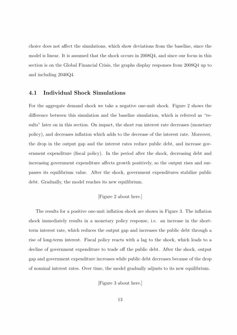
For the aggregate demand shock we take a negative one-unit shock. Figure 2 shows the
difference between this simulation and the baseline simulation, which is referred as “re-
sults” later on in this section. On impact, the short run interest rate decreases (monetary
policy), and decreases inflation which adds to the decrease of the interest rate. Moreover,
the drop in the output gap and the interest rates reduce public debt, and increase gov-
ernment expenditure (fiscal policy). In the period after the shock, decreasing debt and
increasing government expenditure affects growth positively, so the output rises and sur-
passes its equilibrium value. After the shock, government expenditures stabilize public
debt. Gradually, the model reaches its new equilibrium.
[Figure 2 about here.]
The results for a positive one-unit inflation shock are shown in Figure 3. The inflation
shock immediately results in a monetary policy response, i.e. an increase in the short-
term interest rate, which reduces the output gap and increases the public debt through a
rise of long-term interest. Fiscal policy reacts with a lag to the shock, which leads to a
decline of government expenditure to trade off the public debt. After the shock, output
gap and government expenditure increases while public debt decreases because of the drop
of nominal interest rates. Over time, the model gradually adjusts to its new equilibrium.
[Figure 3 about here.]
13

For the public debt shock, a positive one-unit shock is applied, and Figure 4 summarizes
the results. The immediate effect is an increase of the output gap since debt is treated as
net wealth. Monetary policy jumps in by raising both the nominal long-term and short-
term interest rate, while fiscal policy results in a reduction of government expenditure.
In the impulse period, the output gap falls after the instantaneous increase because of
the jump of nominal interest rates and the decreasing government expenditure. After the
shock, with low interest rates, the output gap and government expenditure start rising,
while the public debt falls. Both policies are relaxed over time and the model gradually
reaches a new equilibrium.
[Figure 4 about here.]
4.2 The Global Financial Crisis
To mimic the Global Financial Crisis we employ a combined shock. An aggregate demand
shock and a public debt shock are combined with different weights. In reality, the GFC
does not stop shortly after its occurrence, and its direct influence last more than a year.
Therefore, different from the single shock simulations that have only one shock in 2008Q4,
the shock period is prolonged to the 2008Q4–2009Q4 period.
Figure 1 in Section 3.2 shows that the government expenditures and public debt start
increasing from the end of 2008 onwards, whereas the output gap falls substantially during
the same period. Our simulations match these stylized facts. After some experimentation,
we set the weight of the aggregate demand shock to 1.5 and the weight of the public debt
shock to 3. The size of this combined shock is huge, possibly invoking the Lucas critique.
We make the strong assumption that the linear character of the model and the ‘deep,
structural’ parameters underlying the economy are not affected by the shock.
[Figure 5 about here.]
14
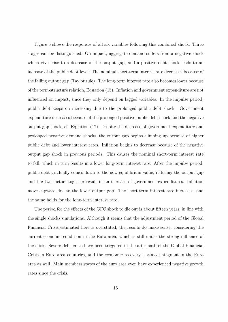
Figure 5 shows the responses of all six variables following this combined shock. Three
stages can be distinguished. On impact, aggregate demand suffers from a negative shock
which gives rise to a decrease of the output gap, and a positive debt shock leads to an
increase of the public debt level. The nominal short-term interest rate decreases because of
the falling output gap (Taylor rule). The long-term interest rate also becomes lower because
of the term-structure relation, Equation (15). Inflation and government expenditure are not
influenced on impact, since they only depend on lagged variables. In the impulse period,
public debt keeps on increasing due to the prolonged public debt shock. Government
expenditure decreases because of the prolonged positive public debt shock and the negative
output gap shock, cf. Equation (17). Despite the decrease of government expenditure and
prolonged negative demand shocks, the output gap begins climbing up because of higher
public debt and lower interest rates. Inflation begins to decrease because of the negative
output gap shock in previous periods. This causes the nominal short-term interest rate
to fall, which in turn results in a lower long-term interest rate. After the impulse period,
public debt gradually comes down to the new equilibrium value, reducing the output gap
and the two factors together result in an increase of government expenditures. Inflation
moves upward due to the lower output gap. The short-term interest rate increases, and
the same holds for the long-term interest rate.
The period for the effects of the GFC shock to die out is about fifteen years, in line with
the single shocks simulations. Although it seems that the adjustment period of the Global
Financial Crisis estimated here is overstated, the results do make sense, considering the
current economic condition in the Euro area, which is still under the strong influence of
the crisis. Severe debt crisis have been triggered in the aftermath of the Global Financial
Crisis in Euro area countries, and the economic recovery is almost stagnant in the Euro
area as well. Main members states of the euro area even have experienced negative growth
rates since the crisis.
15
[Figure 6 about here.]
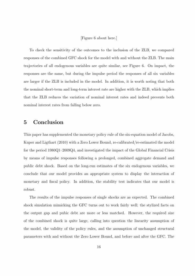
To check the sensitivity of the outcomes to the inclusion of the ZLB, we compared
responses of the combined GFC shock for the model with and without the ZLB. The main
trajectories of all endogenous variables are quite similar, see Figure 6. On impact, the
responses are the same, but during the impulse period the responses of all six variables
are larger if the ZLB is included in the model. In addition, it is worth noting that both
the nominal short-term and long-term interest rate are higher with the ZLB, which implies
that the ZLB reduces the variation of nominal interest rates and indeed prevents both
nominal interest rates from falling below zero.
5 Conclusion
This paper has supplemented the monetary policy rule of the six-equation model of Jacobs,
Kuper and Ligthart (2010) with a Zero Lower Bound, re-calibrated/re-estimated the model
for the period 1980Q1–2009Q4, and investigated the impact of the Global Financial Crisis
by means of impulse responses following a prolonged, combined aggregate demand and
public debt shock. Based on the long-run estimates of the six endogenous variables, we
conclude that our model provides an appropriate system to display the interaction of
monetary and fiscal policy. In addition, the stability test indicates that our model is
robust.
The results of the impulse responses of single shocks are as expected. The combined
shock simulation mimicking the GFC turns out to work fairly well; the stylized facts on
the output gap and pubic debt are more or less matched. However, the required size
of the combined shock is quite large, calling into question the linearity assumption of
the model, the validity of the policy rules, and the assumption of unchanged structural
parameters with and without the Zero Lower Bound, and before and after the GFC. The
16
average adjustment period to the new equilibrium is about fifteen to twenty years for all
six variables. This may seem long, but it does make sense given the current condition of
economic recovery in the euro area. The GFC will haunt the Euro area for some time!
17
References
[1] Bean, C. (1998), “The new UK monetary arrangement: A view from the literature”,
Economic Journal, 108, 1795–1809.
[2] Bekaert, G., S. Cho and A. Moreno (2006), “New-keynesian macroeconomics and the
term structure”, CEPR Discussion Papers 5956, Centre for Economic Policy Research,
London, UK.
[3] Belke, A. and J. Klose (2012), “Modifying Taylor Reaction Functions in Presence of
the Zero-Lower-Bound – Evidence for the ECB and the Fed”, German Institute for
Economic Research Discussion Paper No. 1218.
[4] Berardi, A. (2007), “Term structure, inflation and real activity”, unpublished
manuscript.
[5] Blanchard, O.J. (1985), “Debt, deficits, and finite horizons”, The Journal of Political
Economy, 93, 233–247.
[6] Bracke, T. and M. Fidora (2012), “The macro-financial factors behind the crisis:
Global liquidity glut or global savings glut?”, The North American Journal of Eco-
nomics and Finance, 23, 185–202.
[7] Camarero, M., J. Ordonez and C.R. Tamarit (2005), “The information content
of the euro-area spread: Empirical results using aggregate variables”, unpublished
manuscript.
[8] Estrella, A. and F.S. Mishkin (1997), “The predictive power of the term structure of
interest rates in Europe and the united states: Implications for the European central
bank”, European Economic Review, 41, 1375–1401.
18

[9] Fagan, G., J. Henry and R. Mestre (2005), “An Area Wide Model (AWM) for the
euro area”, Economic Modelling, 22, 39–59.
[10] Gerlach, S. and J. Lewis (2010), “The Zero Lower Bound, ECB Interest Rate Policy
and the Financial Crisis”, DNB Working Paper No. 254.
[11] Fukunaga Ichiro, Naoko Hara, Satoko Kojima, Yoichi Ueno and Shunichi Yoneyama
(2011), “The Quarterly Japanese Economic Model (Q-JEM): 2011 Version”, Bank of
Japan Working Paper No. 11-E-11.
[12] Jacobs, J.P.A.M., G.H. Kuper and J.E. Ligthart (2010), “The dynamic macroeco-
nomic effect of monetary and fiscal policy interaction”, mimeo, University of Gronin-
gen.
[13] Kirsanova, T., S. J. Stehn and D. Vines (2005), “The interaction between fiscal policy
and monetary policy”, Oxford Review of Economic Policy, 21, 532–564.
[14] Lane, P.R. and G.M. Milesi-Ferretti (2010), “The cross-country incidence of the global
crisis”, IMF Working Paper: WP/10/171, Washington, DC USA.
[15] Moshirian, F. (2011), “The global financial crisis and the evolution of markets, insti-
tutions and regulation”, Journal of Banking & Finance, 35, 502–511.
[16] Paredes, J., D.J. Pedregal and J.J Perez (2009), “A quarterly fiscal database for the
euro area based on intra-annual fiscal information”, European Central Bank (ECB)
working paper No. 1132.
[17] Reifschneider, D. and J.C. Williams (2000). “Three lessons for monetary policy in a
low-inflation era”, Conference Series ; [Proceedings], Federal Reserve Bank of Boston,
936–978.
19

[18] Rudebusch, G.D., B.P. Sack, and E.T. Swanson (2007), “Macroeconomic implications
of changes in the term premium”, The Federal Reserve Bank of St. Louis Review, 89,
241–269.
[19] Rudebusch, G.D. and T. Wu (2008), “A macro-finance model of the term structure,
monetary policy and the economy”, The Economic Journal, 118, 906–926.
[20] Shahrokhi, M. (2011), “The global financial crises of 2007-2010 and the future of
capitalism”, Global Finance Journal, 22, 193–210.
[21] Taylor, J. (1995), “The monetary transmission mechanism: An empirical framework”,
Journal of Economic Perspectives, 9, 11–26.
[22] Williams, J. C. (2010), “The Zero Lower Bound: Lessons from the past decade”,
in Lucrezia Reichlin and Kenneth West, editors, NBER International Seminar on
Macroeconomics 2009, University of Chicago Press, Chicago, 367-375.
[23] Yaari, M. (1965), “Uncertain life time, life insurance and the theory of the consumer”,
Review of Economic Studies, 132, p.137–150.
20
Figure 1: Time series of endogenous variables (1980-2009)
21
Figure 2: Aggregate Demand Shock Simulation (2008-2040)
22

Figure 3: Inflation Shock Simulation (2008-2040)
23
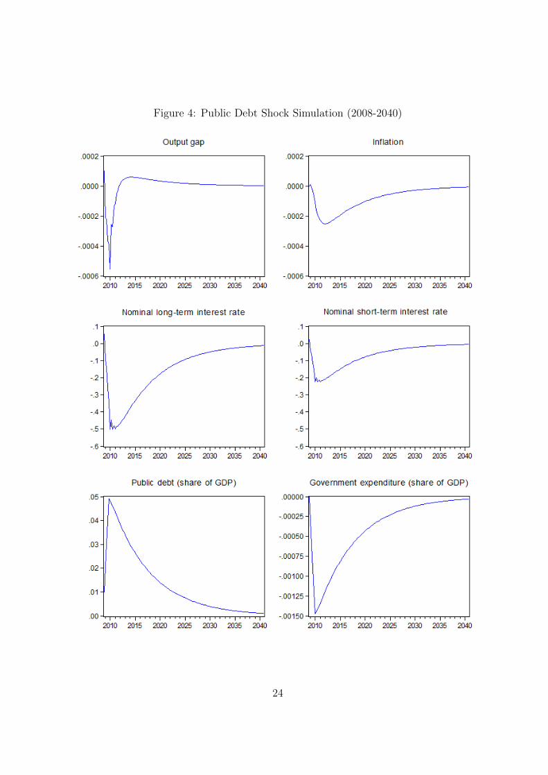
Figure 4: Public Debt Shock Simulation (2008-2040)
24

Figure 5: Combined GFC shock
25
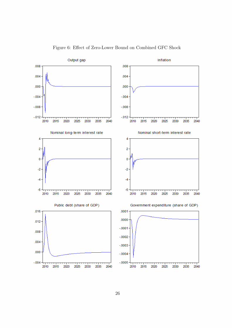
Figure 6: Effect of Zero-Lower Bound on Combined GFC Shock
26
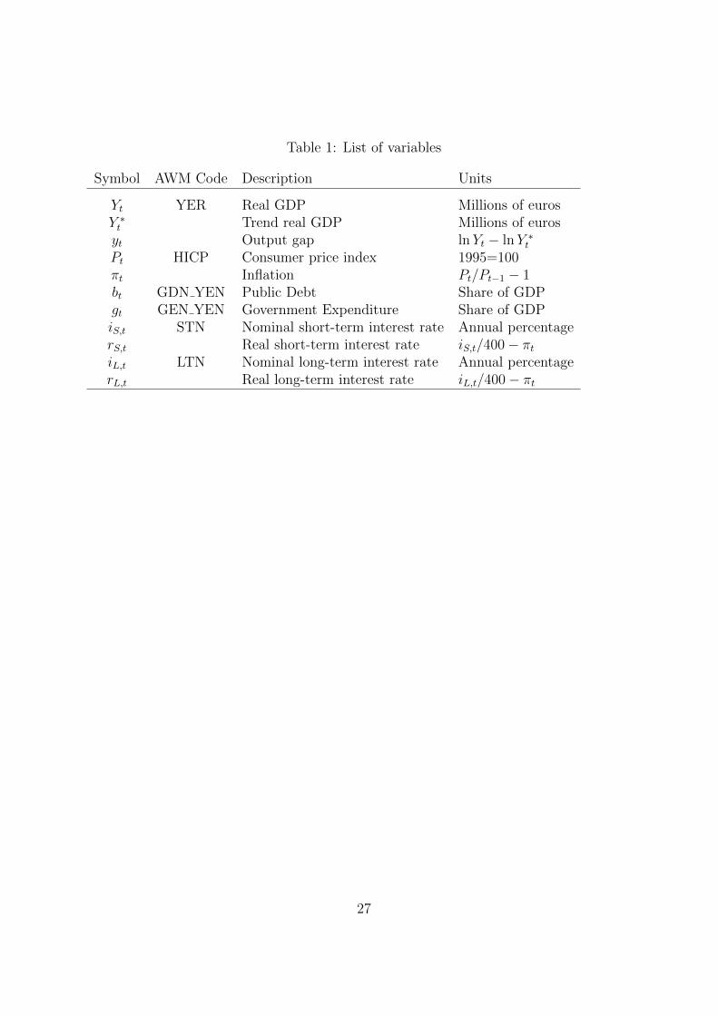
Table 1: List of variables
Symbol AWM Code Description Units
Yt YER Real GDP Millions of eurosY ∗t Trend real GDP Millions of eurosyt Output gap lnYt − lnY ∗tPt HICP Consumer price index 1995=100πt Inflation Pt/Pt−1 − 1bt GDN YEN Public Debt Share of GDPgt GEN YEN Government Expenditure Share of GDPiS,t STN Nominal short-term interest rate Annual percentagerS,t Real short-term interest rate iS,t/400− πtiL,t LTN Nominal long-term interest rate Annual percentagerL,t Real long-term interest rate iL,t/400− πt
27

School of Economics and Finance Discussion Papers
2013-15 Equity market Contagion during the Global Financial Crisis: Evidence from the World’s Eight Largest Economies, Mardi Dungey and Dinesh Gajurel
2013-14 A Survey of Research into Broker Identity and Limit Order Book, Thu Phuong Pham and P Joakim Westerholm
2013-13 Broker ID Transparency and Price Impact of Trades: Evidence from the Korean Exchange, Thu Phuong Pham
2013-12 An International Trend in Market Design: Endogenous Effects of Limit Order Book Transparency on Volatility, Spreads, depth and Volume, Thu Phuong Pham and P Joakim Westerholm
2013-11 On the Impact of the Global Financial Crisis on the Euro Area, Xiaoli He, Jan PAM Jacobs, Gerald H Kuper and Jenny E Ligthart
2013-10 International Transmissions to Australia: The Roles of the US and Euro Area, Mardi Dungey, Denise Osborn and Mala Raghavan
2013-09 Are Per Capita CO2 Emissions Increasing Among OECD Countries? A Test of Trends and Breaks, Satoshi Yamazaki, Jing Tian and Firmin Doko Tchatoka
2013-08 Commodity Prices and BRIC and G3 Liquidity: A SFAVEC Approach, Ronald A Ratti and Joaquin L Vespignani
2013-07 Chinese Resource Demand and the Natural Resource Supplier Mardi Dungy, Renée Fry-McKibbin and Verity Linehan
2013-06 Not All International Monetary Shocks are Alike for the Japanese Economy, Joaquin L Vespignani and Ronald A Ratti
2013-05 On Bootstrap Validity for Specification Tests with Weak Instruments, Firmin Doko Tchatoka
2013-04 Chinese Monetary Expansion and the US Economy, Joaquin L Vespignani and Ronald A Ratti
2013-03 International Monetary Transmission to the Euro Area: Evidence from the US, Japan and China,
Joaquin L Vespignani and Ronald A Ratti
2013-02 The impact of jumps and thin trading on realized hedge ratios? Mardi Dungey, Olan T. Henry, Lyudmyla Hvozdyk
2013-01 Why crude oil prices are high when global activity is weak?, Ronald A Rattia and Joaquin L Vespignani
Copies of the above mentioned papers and a list of previous years’ papers are available from our home site at http://www.utas.edu.au/economics‐finance/research/