,

, ' I

1 ' 1

I

I

'I

NASA Technical Memorandum 102036 ICOMP-89- 1 1

On the Equivalence of a Class of Inverse Decomposition Algorithms for Solving Systems of Linear Equations

Nai-kuan Tsao Wayne State University Detroit, Michigan

and Institute for Computational Mechanics in Propulsion Lewis Research Center Cleveland, Ohio

(I!4ASA-TM-102036) O B THE EQUIVALENCE OP A CLASS OF INVERSE DECOHPOSXTION ALGORITHdS FOB SOLVING SYSTEBS OF L I N E A R EQUATIONS

(NASA. L e v i s Besearch Center) 28 pCSCL 12A Unclas

N89 - 2 48 65

G3/64 0210306 I May 1989

1 ;

LEWIS RESEARCH CENTER

! '

https://ntrs.nasa.gov/search.jsp?R=19890015494 2018-05-17T16:24:01+00:00Z

On the Equivalence of a Class of Inverse Decomposition Algorithms for Solving Systems of Linear Equations

Nai-kuan Tsao* Wayne State University

Detroit, Michigan

and Institute for Computational Mechanics in Propulsion Lewis Research Center

Cleveland, Ohio 44 135

Summaq

A class of direct inverse decomposition algorithms for solving system of linear equations is

prcscntcd. Their behavior in the presence of round-off errors is analyzed. It is shown that undcr

S O I T K mild rcstrictions on their implementation, the class of direct inverse decomposition algorithms

prcxritcd arc equivalent in terms of our crror complcxity measures.

'This work was supported in part by the Space Act Agreement C99066G while the author was visiting ICOMP. NASA Lewis Research Center.

1

1. Introduction

Given a system of linear equations

A x = b,

ivhere

the solution vector x can he found as

x = .4-'b

providcd A is non-sinbwlar. Using direct methods the A-I is usually decomposed as a product of

elementary matrices which reduces the original A to an identity matrix. This is true whether the

method selected is of the Gaussian Elimination type which triangularize A or the Gauss-Jordan type

in which diagonalization of A takes place. In actual computation the decomposed A - l is of course

only an approximation to the exact one due to round-off errors incurred during the execution of

the computational steps of the speciiic method chosen. Since there are many variations in this class

of decomposition methods, one wonders whether one variation is "better" than the other in terms

of accuracy of the computed solution.

In this papcr we show, under mild restrictions on the implcmcntation of some algorithms,

that all decomposition methods are "equivalent" in terms of our error complexity measurus. Some

prcliminary rcsults are presented in Section 2. The classification and analysis of decomposition

methods are given in Section 3.

2. Some Preliminary Results

Given a normalized floating-point system with a t-digit base p mantissa, the foUoiving

cqucitinns can be assumed to facilitate the error analysis of general arithmatic exprcssions using only

+, -, t , or / operations[ 11:

2

whcre

- /? - for rounded operations

/?I-' for chopped operations I A I _ < l + u , US{ '

and x and y are given machine floating-point numbers and J(.) is used to denote the computed

lloating-point result of the given arbmment. We shall call A the unit A -factor.

In gcneral one can apply (2.1) repeatedly to a sequence of arithmetic steps, and the computcd

result z can be expressed as

(2.2)

j= 1

whcrc each z,,, or zd, is an exact product of error-free data, and Ak stands for the product of k pos-

sibly different A-factors. We should emphasize that all common factors between the numerator and

denominator should have bccn factored out before z can be expressed in its final rational form of

(2.2). Following [2], we shall henceforth call such an exact product of error-free data a basic tcrm,

or simply a term. Thus A(zJ or A(z,) is then the total number of such terms whose sum constitutes

z, or z,, respectivcly, and u(z,) or u(zd,) gives the possible number of round-off occurrences during

thc computational process. As an example, consider the solution of two linear equations in two

variables as follows:

Q X ~ + bx2 c

d x , +ex2 = f

The exact solution x, can be found as

The computed x, is the result of the following expression:

3

dc A3 afA - dcA3

e A - 7 db aeA - dbA3 - - f A - 7

x2 =

which is of the form of (2.2). We defme the following two measures: I

i maximum error complexity:

I cumulative error complexity:

(2.3) i= 1 j = 1

Different algorithms used to compute the same z can then be compared using the above error

complexity mcasures and the number of basic terms created by each algorithm.

For convenience we will use Fd and Z, to represent the 3-tuples (A(zd), a(z,), s(zd)} and

{2(z,,), a(z,,), ~(z,,)} , respectively, so that the computed z of (2.2) is fully characterized by

In division-free computations any computed z will have only the numerator part 2,. The

I follo\ving lemma is useful in dealing with intermediate computed results:

4

Proof. The results can be obtained easily by expressing x and y as

i= 1 j = 1

and applying (2.3j, (2.4) and the definition of A(zJ to find Z,. Q.E.D.

71ic unit A-factor is then defined as

- ( 2 . h ) A { l,l,l}.

One can obtain casily using Lemma 2.1 to get

-i (2.5b) A = { l,i,g.

For general floating-point computations, we have the following lcmma:

5

Proof. First we apply (2.1) to each case and obtain

‘Thc rcsults can then be obtained easily by using (2.3) and (2.4). Q.E.11.

Often oxie needs to add up an extended sum given by

(2.6)

The order of summation certainly has to be specified. One would like to select an order to mini-

mize the incurred additional error complexities of the final computed z. We consider the following

four strategies.

I f the items are added recursively in parallel by divide-and- conquer, then the strateg is called

left-heavy if

fk/21 A

= xi, z2 =

i= rw21 +I c i= 1

Similarly the strategy is called right-heavy if

If the items are summed up in sequential order, then we have the common stratcgies of l ~ , f t -

to-right or right-to-left. We have the following useful lemma:

6

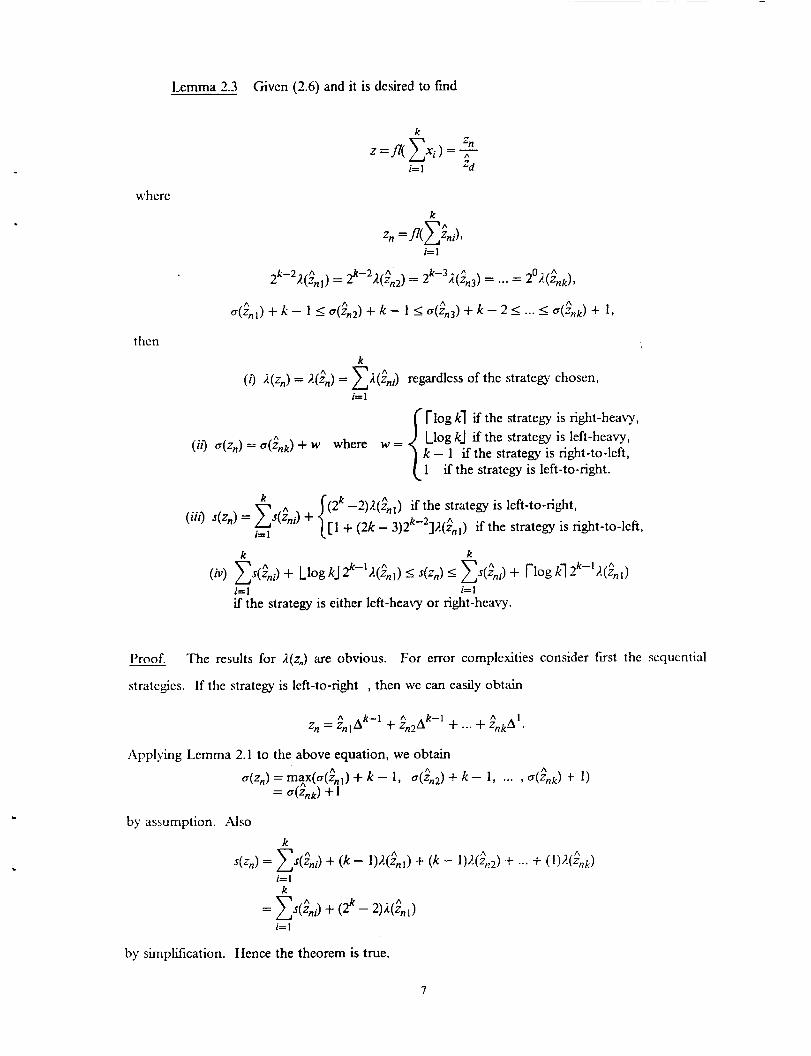
Imnma 2.3 Civen (2.6) and it is desired to find

k &n

i= 1 "d z =fl( E X i ) = ;

where

tlicn k

( i ) 2(zn) = A ( i n ) = EA(̂ z,J regardless of the strategy chosen, i= 1

( rlog kl if the strateby is right-heavy, Llog kJ if the strategy is left-heavy, k - 1 if the strategy is right-to-left,

(ii) u(zn) = u(Snk) + w where w =

(1 if the strategy is left-to-right.

(2k -2)A(;nl) if the strategy is left-to-right, [l + (2k - 3)2k-2]A($n,) if the strategy is right-to-left,

k k-1 A

k

(iii) s(zn) = + i= 1

k

(iv) E.&) + Llog kJ f - l A ( $ n l ) I s(zn) 5 + flog k'l2 3.(znl) i= 1 i= I if the strategy is either left-heavy or right-heavy.

Proof.

stratcgics. If the strategy is left-to-right , then we can easily obtain

The results for A(z,,) are obvious. For error complexities consider first the scqucntial

Applying Lcmrna 2.1 to the above equation, we obtain

by assumption. N s o

i= 1

by simplifcation. Ilence the theorem is true.

7

By rcpeated application of Lemma 2.1 we have certainly

.(z,) = a($n&) + k - 1.

Also

\vhich can also be simplified to the desired form. Hence the theorem is true in this case. For the

parallel strategies, the computed z,, can be expressed as

A ' A ' A . Z, = znlAJ' + zn2AJ2 + ... + ZnkAJk

ivhere

j , = rlog k1 rjz 2 ... 2 j k = Llog kJ if the strategy is left-heavy,

j , = Llog kJ sj2 I ... sjk = rlog kl if the stratcgy is right-heavy,

Now if the strategy is right-heavy, it is obvious that

= + nos ki.

If the strategy is left-heavy, then by assumption we have

+ Llog kJ 2 a(.&) + Llog kJ + k - i 2 + rlog k1 for i -= k Hence

o(z,,) = 0 ( 2 ~ k ) + Lbg kJ .

The cumulative error complexity results are obvious. This complctes our proof. Q.E.D.

Now from the results of Lemma 2.3 we see obviously that u(z,,) will be minimal if the strategy

is Icft-to-right. For s(zJ we see that

2& -2 I rlog k1 2k-' I [ 1 + (2k - 3)2k-2], for k > 3 or k = 2.

Furthermore for k = 3 then we have

2 A 2 A i n 1 A + zn2A + zn3A if the strategy is left-heavy, $,,]A + &A2 + 2n3A2 if the strategy is right-heavy.

Hence

8

( f in( .$ , ) if the strategy is left-heavy,

I .

7R(;,,,) if the strategy is right-heavy, 6R(in1) if the strategy is left-to-right, 4%) = & I ) + 4 2 ) + 4 4 3 ) f

(7R($n1) if the strategy is right-to-left.

Thus the left-to-right strategy gives us, in all cases, the minimal cumulative error complexity also

in thc computed rcsult. We conclude with the following theorem:

'Ihcorem 2.1 If (2.6) is to be computed 'and the conditions specified in Lzmma 2.3 are sat-

isfied, then one should choose the strategy left-to-right in order to mlllimize both the maximum

and cumulative error complexity of the computed extended sum.

3. Inverse Decomposition Methods

'To find the inverse decomposition, onc applies a sequence of clementary trasformations to

the matrix A so that zeroes are creatcd in the lower and upper parts of thc matrix. The final reduced

matrix is of course the identity matrix sa that an implicit A-I can be obtained as a product of the

scqucnce of elementary matrices which can then be applied to b to obtain the desired solution

x = A-Ib . In general a large collection of methods can be classified as the usual triangular de-

composition of A into a product of lower and upper triangular matrices followed by explicitly or

implicitly inverting the calculated triangular matrices. To see this consider the diagonalization of

an ,1' x 1V matrix. The Gauss-Jordan mcthod

would crcate a sequence of matrices C,, C,, ... and C, such that

We shall assume that pivoting is not necessary.

N T CN ... C , C , A = D , C i = I N - 1 cjejei

j = 1 , j#i

wherc IN and e: represent the N x N identity matrix and the transpose of the i-th column of the

identity matrix , respectively. The matrix C, is chosen such that the transformed matrix

C,C, .,... C,A will have all its off-diagonal elements of the first i columns zeroed. It is also obvious

that the matrix C, depends on the previously generated c-l, C,-2, ..., C, and A . Kow C, can be ex-

pressed as

9

N i- I T 7' C.=I- ( I .= I dl . 1,I.l. , L - 1 - ,v - C cjicjei , [li = 1, - z c j i q r i

j=i+ 1 j = 1

whcre U, and L, represent, respectively, the upper and lower part of C,. Furthcrmore we can easily

show by induction that

Hence

U - I L - I A = D ,

Since the steps in L-lA describe the elimination stage of the Gaussian Elimination mcthod in COII-

vcrting A to an upper triangular form and the subsequent U-'(L-'A) is the result of a fonvxd

elimination process to crcatc zeroes in the uppcr triangylar L-lA by columns, the Gauss-Jordan

mcthod is therefore numerically equivalent to the elimination stage of Gaussian Elimination

method followed by a forward-elimination process to diagonalize the intermediate upper triangular

form. More precisely, the Gaussian Elimination method explicitly finds a matrix L whose inverse

L-l, in implicit produd form, is used to reduce the matrix A to an upper triangular matrix U such

that

A = L U , L - ' A = LI

The Gauss-Jordan mcthod creates the same L and an explicit unit-diagonal upper triangular matrix

%I such that

ML-' A = D.

llcnccforth we shall restrict our attention to the class of methods by which the matrix .4 is

decomposed frst into a product of lower and upper triangular matrix in one of the following two

forms:

(3. la) A = L U

10

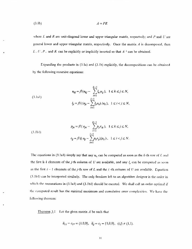
(3.1 b) A = P R

ishere f and R are unit-diagonal lower and upper triangular matrix, rcspectvcly; and f' arid L! are

gcncral lower and uppcr triangular matrix, respcctively. Once the matrix A is dccomposcd, then

I, , [,! , P and R can be explicitly or implicitly inverted so that ,4-' can be obtained.

Expanding the products in (3. laj and (3.1 bj explicitly, thc dccompositions can be obtained

by the following rccursive equations:

(3.1 a 1 )

(3.lbl)

k- 1

u k j = j l ( a k j - ~ I k l u o ) , l S k l j l N ,

$i =fl( (aji - ~ $ p l i ) /ui i ) , 1 I ic j I N ,

I= 1 i- 1

I= 1

The equations in (3.lal) simply say that any uk, can bc computed as soon as the k-th row of L and

the f i n t k-1 clcmcnts of the j-th column of U arc available, and any $, can be computed as soon

as the first i - 1 clements of the j-th row of L and the i -th column of LI arc available. Equatinn

(3. lhl) can be interpreted similarly. The only freedom left to an algorithm designer is the ordcr in

u hich the summations in (3.lal) and (3.lbl) should hc excutcd. Wc shall call ;m ordcr optimal if

thc coniputcd result has the minimal maximum md cumulative error complcsitics. \\'e have the

follo\i.ing theorem:

Thcorcm 3.1 Let the given matrix A be such that

- - a l l =cl~={l,O,O}, ug=cl ={l,O,O}, ( i j ] f ( l , l ) .

1 1

'Ihc optimal ordcr to compute the summations in (3.lal) and (3. lbl) is the left-to-right strategy for

thcir evaluation using the explicit expressions given by

and the computed ukJ I 4, lpJk and rl, satisfy

where

Proof. See Appendix I.

Dy Theorem 3.1 we see that all variations of the class of methods for decomposing A into

LU or PR are equivalent among those methods of their respective class in terms of our complexity

mcasurcs as long as the left-to-right strategy is adhercd to in the evaluation of (3.la2) or (3.lb2).

Two variations each for the decompositon of A into forms given by (3.la) and (3.lb) are listed

bclour :

Algorithm G {Gaussian elimination for A = L U }

for i = 1 to N - 1 do f o r j = i + 1 to N d o

=fl ( ' J l / ' U )

f o r k = i + 1 t o N d o ' J k =fl( ' J k - 4, 'tk

for k = 1 to N do f o r j = k t o N d o

' k j = ' k ]

12

Algorithm 111, { Doolittlc mcthod for A = L L ' }

for j = 1 to A' do f o r i = 1 t o j - 1 do

for k = j to N d{?l

, - I

4, =f7 ( ( - I/Auki ) / t c i ,

J - 1

yk =/7 ( ' J k - E{k!?tk ,= I

I . Illgorithm Cil (Gaussian 1:limination for A = P R }

f o r i = 1 to N - 1 do for k = i + 1 to A' do

' i k =fl( atk/at, for j = i + 1 to ,V d o

' J k =fl( ' J k - ',t ' r k ) for k = 1 to N do

fo r i = k to N do P j k = a,k

Nporithm CR

for k = 1 to N do

(Crout method for A = PR}

f o r j = 1 to k do J-1

P & ) = f 7 ( ' k J - ~ P k m ' m J )

for j = k + I to xi0 1-1

' k j =fl( ( ' k j - C P k m ' m , ) / P k k m=l

\Vc are now rcsdy to find the inverses of L, U, P, R either implicitly or explicitly. Givcn f/ ,

thc product form of L-I can be obtained without additional computation as

(3.2a)

( 3 . 3 )

On the othcr hand, onc can also obtain explicitly a lowcr unit-diagonal matrix hl such that

\tf, = I, and

(3 .2)

13

Note that (3.2a), (3.2b), ( 3 . 2 ~ ) ~ and (3.2d) can be regarded as methods creating zeroes in the given

L by column-wise foward , row-wise forward, column-wise backward, and row-wise backward

elimination, respectively.

Solving for hfL = I, wc fmd that

k- 1

mi+kj =fl( 4 + k j - cr?$+kj+j'i+jj ), 1 I k I N - 1 , 1 I i I N- k. j = I

In other words, mi+,j depends on those elements of the (i+ k) -th row of M to its right, as well as

( + k , r and thosc above it in the i-th column of L. A proper algorithm is the following:

A 4 ~ o r i i h m M

for k = 1 to N - 1 do f o r i = 1 to A ' - k do

j = i + k m,, =fl( I,, - m,d-l$-l,, - ... - m,.,+,l+~,~ 1

We have the following thcorcm:

,_ I heorcm 3.2a Given L whose error complexities satisfy Theorem 3.1, then the optimal or-

der to f i d h4 using Algorithm M is again thc left-to-right strategy for the summations. The com-

puted ,I! has error complexities given as

j= 1 j= 1

Proof. See Appendix 11.

14

.

Since L is applied t o ,4 and I,-I,4 = CI, the smie operations need to be ripplicd to the right

hand side vector h in solving Ax = h so that thc reduced system I'x =/c:rn lw \olLcd I.itcr \\ hcrc

f= L-'6. One natural question is whcthcr (3 .2a) through (3.2d) are equivalent in the scnse that the

computed fusing any of them will have the same error complesities. For (3 .21) and (3.2b) this is

true as wc can simply augment A with b as its (iV + 1)-st column and a decomposition of A = L L J

can be perfonncd with U being a trapezoidal matrix hairing f as its last column. For (3 .2~) and

(3.2d) the results of Theorem 3.2a can be applied and we can easily obtain the following thcorcm

by induction:

Theorem 3 . 3 If the given right hand side vector b is such that h, = { I,O,O}, then the com-

putcd

using any one of (3.2a) through (3.2d) is such that

- A=U,.N, I < i < N

provided the summations used to evaluateJ in (3.2b) and (3.24 are carried out using the left-to-

right strategy in the following expressions:

(3 .Y 1) ~ = J ( b j - n i i , i - l b j - I -mi , i -2b i -2 - . . . - rn i lb l ) , I S i < N - - 1.

TO find P-1 the situation is similar. Two different forms of P-I can be found without addi-

tional cffort:

( J .?>3)

(3.3b)

15

( 3 . k )

i- 1 T

I J

j = 1

T T D, = I , - qei + 4iqei , p1;l = I , - pjiejei , P;' = I , ~ - ..e eT . j=i+ 1

L'sing an additional O(N2) divisions one can also obtain the following two forms easily:

Sotc the above are fonvard type of algorithms. In (3.3a) and (3.3b) P is gradually reduced

to an idcntity matrix, whcrcas in (3 .3~) and (3.3d) it is reduced first to a diagonal matrix. If we

prc-multiply P first by D-', then the new matrix becomes a unit-diagonal lower triangular matrix

and four ncu. forms similar to ( 3 . 2 ) through (3.2d) can be dcrived. By Thcorem 3.2b wc know that

thcy arc cquivalcnt among thcmsclves. We shall only give one of thcm in detail:

N

( 3 . k ) i

1 ~ i i ; J l y P can also be reduccd first to diagonal matrix by backward type of algorithms. \\'e

h S V C

(3.3f)

16

I

1 -

I -

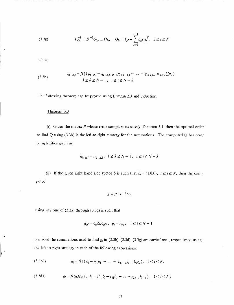
(3.3g)

where

The following theorem c.m be proved using Lxmma 2.3 and induction:

Theorem 3.3

(i) Given the matrix P whose error complexities satisfy Theorem 3.1, then the optimal order

to find Q using (3.3h) is the left-to-right strategy for the summations. The computed Q has crror

complcxitics 5 vcn as

(ii) If the given right hand side vector b is such that b, = { 1,0,0}, 1 I is A’, then the coni-

p t c d

using a n y one of (3.3a) through (3.3g) is such that

- - - 51\1=cNA/cN*, g i = r i N , I l i l N - 1

pro\.idcd the summations used to find g, in (3.3b), (3.3d), (3.3g) arc carried out , respectively, using

the left-to-riglit strategy in each of the following expressions:

(3.3hI) g i = f l ( ( b i - P i , g l - ... - Pi,i-lgi-1)lpii)! 1<is!+’,

17

Methods for finding R-' and U-' arc similar to those for finding L-' and PI, respectively.

We shall simply list them and give the resulting theorems without proofs.

(3.44 KF; = M', ... M', = I N - j = 1

where M' is a unit-diagonal upper triangular matrix computed by the follouing formula:

m'i,i+k =fl( "j+k - m'i,i+lri+,,i+k - ... - m'. i , r+k- l~+k-I , i+k) . 9 (3.34 l < k S N - 1 , 1 <is ,+ ' -k .

'l'hcorcm 3.4

( i ) Given R whose error complexities satisfy Theorem 3.1, thcn the optimal order to evaluate

( 3 . 4 ~ ) is thc left-to-ri&t strategy. The computed M' is such that

(ij) given g \.{,hose error complexities satisfy Theorem 3.3, thcn the computcd

18

using .any onc of (3.4:;) through (3.4d) is such that

provided the summations used to evaluate x, in (3.4b) and (3.4d) are carried out hi optknal order

of thc Icft-to-right strategy , rcspcctively, using the following cxpressions:

(3.3b1) xN=gh:r - 1 y. = j j ' (g. I - r. r,,~xN - ... - r . . 1 , 1 + 1 x . I + l ) , 1 I i I 12: - 1,

(3.3d I ) x . =j l (g . - In'. I,I+lgi+l . - ... - m'iNg,,l) , 1 5 i s N .

\lethods for U-':

(3. Sa)

( 3 . 3 ) )

i- 1 N T

Ir N -- C uijeicj . U, = I , - eiei + uiieiei , U ~ ; = I,,, - Ci$icyi , ~ 1 - l = I j= 1 j=i+ 1

T T 1 T

( 3 . k )

\v h c rc

19

t l j i = j7 ( uij/3, ) , D , = diag [uii , ... , u,$rN].

(3.59

(3.5s)

\r.hcrc Q' is a unit-diagonal upper triangular matrix computed by the follo\ving formula:

Thcorem 3.5

(i) Given the matrix U whosc error complexities satisfy Theorem 3.1, then the optimal ordcr

to fmd Q' using (3.5h) is the lcft-to-right strategy for the summations. ?he computed Q' has crror

complcxitics given as

(ii) Given /\\hose error comp1c;uities satisfy Theorem 3.2b, then the computed

using any one of (3.5a) through (3.5g) is such that

20

pro\ided the summations used to evaluate x', in (3.Sb), (3.5d), (3.5g) arc carried out, rcspcctivclp,

using the left-to-right strategy in each of the following expressions:

(3.Sbl) x'[=/I( ( A - 11. IN. Y" - ... - ui,i+]x'i+l ) / U i i ) , 1 I i < N ,

(3.53 1) xri = f 7 0 , , . / ~ ~ ~ ) , yi = / l ( f i ' - d i d N - ... - zli,i+lyi+l ) , 1 I i I N ,

By Theorem 3.5 wc conclude that the class of invcrse decomposition methods bawd on

finding the tri;mgulcir factors of the matrix A followed by cxplicitly or implicitly invcrting thc tn-

angwlar factors are cquivalcnt among thcmselves in terms of our error complexity measures.

.

21

References

[ I ] J . € I . Wilkinson, Rounding Errors in Algebraic Processes, Englewond Cliffs, NJ: Prenticc

rm, 1963.

[2]

metic expressions, SIAhI J. Computing, 8( 1979), pp, 60-72.

V.B. Aggawal and J.W. Burgneier, A round-off error model with applications to arith-

22

Appendix 1. Proof of 'T'hcorem 3.1

I lcnce

and thc thcorcm is true. Assume the theorem is true for k = i = r - 1. For k = i = r we assume

that in thc computation of uk, the given /k, and ut, for 1 I t I k - 1 are calculated by the optllnsl

nrdci and so u,, can be considered as the computed result of

;Tow by assumption

I lcrice

Sow if cxact additions wcre possible, then

. k 1 z = - c z n i

zd I= 1

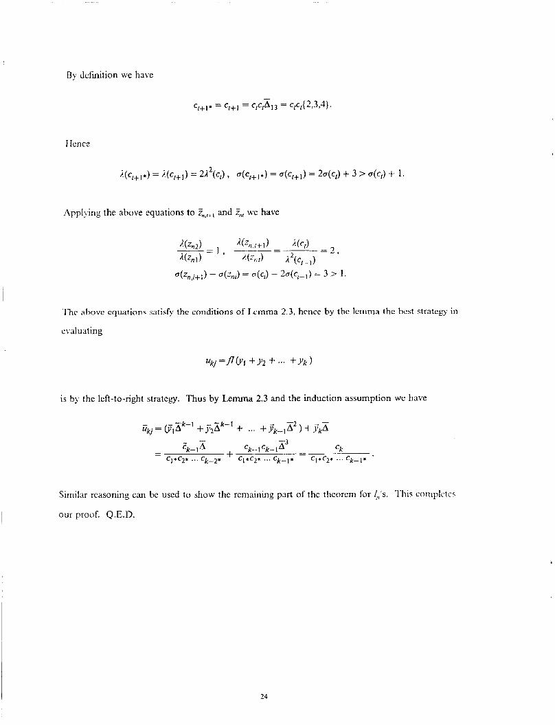
By Jcfiition we have

I lonce

2 i.(C,+1*) = R ( C , + l ) = 22 (CJ , b(cf+l*) = a(cr+l) = 2a(c,) + 3 > a(c,) + 1.

/\pplying the above equations to Z,,,,, and T,,, we have

T h c above cquations satisfy thc conditions of I rmma 2.3, hcncc by the .:nima the hcst stratem in

evaluating

is by the Icft-to-right strategy. Thus by Lmnrna 2.3 and the induction assumption we have

Similar rcasoriing can be used to show thc rcrnaining part of the thcorcni lor 4,’s. l’his cornplctcs

our proof. Q.E.D.

24

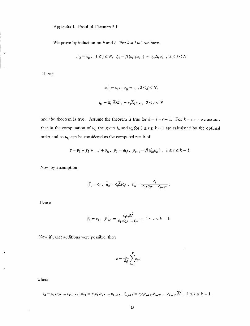
Appendix 1. Proof of 'T'hcorcm 3.1

We prove by induction on k and i. For k = i = 1 we have

ul j = uii, 1 I j 2 h'; l,, =J7(ut l /u l ) = q l A / o l , 2 5 i 5 A'.

I Jence

ill = Z I l ~ / Z l l = CI;I/CI* , 2 I t I :I'

and thc thcorcm is true. A4ssume the theorem is true for k = i = r - 1. For k = i = r we assume

that in the computation of uk, the given /kf and uf, for 1 I t I k - 1 are calculated by the optimal

nrdcr and so ukj can be considered as the computed result of

Xow by assumption

I Icnce

- - C,CI.2 .VI = C] 9 y,+1 = cI*cz* .., 9 1 I t 5 k - 1.

Sow if cxact additions were possible, then

k

I= 1

By dcfmition we have

I lcnce

2 j.(cf+lg) = >.(cl+l) = 21 (c,) , U ( C ~ + ~ * ) = a(cf+l) = 2 4 4 + 3 > c(cf ) + 1.

Applying the above equations to Zn,,+, and Z,, we have

U(zn,i+l) - “(Zni) = “(CJ - 2 O ( C i _ ] ) = 3 > 1

T h e above cquations satisfy the conditions of Lxmma 2.3, hcncc by the Icmma the best stratcEy in

evaluating

is by the left-to-right strategy. Thus by L x m a 2.3 and the induction assumption we have

Similar rcasoriing can be uscd to show the remaining part of the thcorcni for 4,’s. l’his coinplctcs

our proof. Q.E.D.

,

24

2. Government Accession No. NASA TM-102036 1. Report No.

ICOMP-89- 1 1 -

5. Report Date 4. Title and Subtitle

3. Recipient's Catalog No.

On the Equivalence of a Class of Inverse Decomposition Algorithms for Solving Systems of Linear Equations

May 1989

i I

' 9 Performing Organization Name and Address

1 Lewis Research Center , Cleveland, Ohio 44135-3191

1

National Aeronautics and Space Administration

I 8. Performing Organization Report No.

11. Contract or Grant No.

-. 13. Type of Report and Period Covered

' Nai-kuan Tsao I

i

17 Key Words (Suggested by Author@))

Gaussian elimination, Gauss-Jordan method; Triangular decomposition; Error complexity; Doolittle method;

1

I Crout method

E-4785

18. Distribution Statement

Unclassified -Unlimited Subject Category 64

1

Agency Name and Address I

-

Technical Memorandum

I Unclassified Unclassified

I i j Washington, D.C. 20546-0001 I

National Aeronautics and Space Administration 14. Sponsoring Agency Code

I 15 Supplementary Notes

Nai-kuan Tsao, Wayne State University, Detroit, Michigan 48202 and Institute for Computational Mechanics in

Space Act Monitor: Louis A. Povinelli. I 1 I

Propulsion, Lewis Research Center (work funded under Space Act Agreement C99066G). ~

I - 16 Abstract I

I

I A class of direct inverse decomposition algorithms for solving systems of linear equations is presented. Their ' behavior in the presence of round-off errors is analyzed. It is shown that under some mild restrictions on their implementation, the class of direct inverse decomposition algorithms presented are equivalent in terms of our

~

I

error complexity measures. 1

~

I

.

~ ~~ ~

'For sale by the National Technical Information Service, Springfield, Virginia 221 61 NASA FORM 1626 OCT 86