Embed Size (px)
Citation preview

DISCRETE AND CONTINUOUS doi:10.3934/dcdsb.2013.18.2331DYNAMICAL SYSTEMS SERIES BVolume 18, Number 9, November 2013 pp. 2331–2353
ON THE DYNAMICS OF TWO-CONSUMERS-ONE-RESOURCE
COMPETING SYSTEMS WITH BEDDINGTON-DEANGELIS
FUNCTIONAL RESPONSE
Sze-Bi Hsu
Department of Mathematicsand The National Center for Theoretical Science
National Tsing-Hua University
Hsinchu 30013, Taiwan
Shigui Ruan
Department of Mathematics
University of Miami
Coral Gables, FL 33124-4250, USA
Ting-Hui Yang
Department of Mathematics
Tamkang UniversityNew Taipei City 25137, Taiwan
(Communicated by Yuan Lou)
Abstract. In this paper we study a two-consumers-one-resource competing
system with Beddington-DeAngelis functional response. The two consumerscompeting for a renewable resource have intraspecific competition among their
own populations. Firstly we investigate the extinction and uniform persistenceof the predators, local and global stability of the equilibria, and existence of
Hopf bifurcation at the positive equilibrium. Then we compare the dynamic
behavior of the system with and without interference effects. Analyticallywe study the competition of two identically species with different interference
effects. We also study the relaxation oscillation in the case of interference
effects. Finally we present extensive numerical simulations to understand theinterference effects on the competition outcomes.
1. Introduction. In this paper we study a two-consumers-one-resource systemwith Beddington-DeAngelis functional response. The two consumers (predators)competing for a renewable resource (prey) have interference competition amongtheir own populations. The mathematical model takes the following system of
2010 Mathematics Subject Classification. Primary: 37N25, 92D25, 92D40.Key words and phrases. Predator-prey system, Beddington-DeAngelis, extinction, uniform per-
sistence, Lyapunov function, global stability, relaxation oscillations.The research of Sze-Bi Hsu and Ting-Hui Yang are partially supported by National Council of
Science and the National Center for Theoretical Sciences, Taiwan, Republic of China.
The research of Shigui Ruan is partially supported by National Science Foundation (DMS-1022728).
2331
2332 SZE-BI HSU, SHIGUI RUAN AND TING-HUI YANG
three nonlinear ordinary differential equations Beddington [2], DeAngelis et al. [8],Huisman and De Boer [15]:
dx
dt= rx(1− x
K)− m1x
a1 + x+ b1y1y1 −
m2x
a2 + x+ b2y2y2,
dy1
dt= (
e1m1x
a1 + x+ b1y1− d1)y1, (1)
dy2
dt= (
e2m2x
a2 + x+ b2y2− d2)y2
with initial values x(0) = x0 > 0, y1(0) = y10 > 0, y2(0) = y20 > 0.In (1) x(t), y1(t), and y2(t) represent the population density of prey and two
predators respectively at time t. In the absence of predation, the prey grows lo-gistically with intrinsic growth rate r and carrying capacity K. The i-th preda-tor consumes the prey according to the Beddington-DeAngelis functional responsemixyi
ai+x+biyiand its growth rate is eimixyi
ai+x+biyi, where ei is the conversion efficiency coef-
ficient ; mi is the maximal consumption rate; ai is the half-satuation constant andbi measures the intraspecific interference among the population of i-th predator; diis the death rate.
Note that if b1 = b2 = 0 then system (1) is reduced to a system with Hollingtype II functional responses:
dx
dt= rx(1− x
K)− m1x
a1 + xy1 −
m2x
a2 + xy2,
dy1
dt= (
e1m1x
a1 + x− d1)y1, (2)
dy2
dt= (
e2m2x
a2 + x− d2)y2.
Hsu, Hubbel and Waltman [13, 14], Butler and Waltman [5], Keener [18], Muratriand Rinaldi [20], Smith [21], Liu, Xiao and Yi [19], among others, have showedthat system (2) exhibits coexistence in the sense of Armstrong and McGehee [1],that is, for appropriate parameter values and suitable initial population densities(x(0), y(0), z(0)), the model does predicts coexistence of the two predators via alocally attracting periodic orbit. However, system (1.2) cannot be uniformly per-sistent. The case when b1 = 0 and b2 6= 0 was studied in Catrell, Cosner and Ruan[7].
This paper is organized as follows. In Section 2, we study existence and stabilityof equilibria in system (1), including the semi-trivial equilibria( i.e., with survivalof only one predator species ) and the positive equilibrium ( with the coexistence ofboth competing predators). Sufficient conditions for the uniform persistence of thesystem are obtained. In Section 3, we construct a Lyapunov function to establish theglobal stability of the positive equilibrium. We also have similar extinction resultsas those in [14]. In Section 4, we consider the competition of two identical predatorswith different interference effects. In Section 5, we study relaxation oscillations tosystem (1) with r � 1 and bi = O(ε1+µi) where ε = 1/r and µi > 0, i = 1, 2.Numerical simulations are presented to explain the obtained results.
2. Local analysis.
2.1. Subsystems. Consider the following predator-prey system which is a subsys-tem of (1):

TWO-CONSUMERS-ONE-RESOURCE COMPETING SYSTEMS 2333
dx
dt= rx(1− x
K)− mx
a+ x+ byy,
dy
dt= (
emx
a+ x+ by− d)y,
x(0) > 0, y(0) > 0.
(3)
With the scaling:t→ rt, x→ x/K, y → by/K (4)
the system (3) becomes dx
dt= x(1− x)− sxy
x+ y +A,
dy
dt= δy(−D +
x
x+ y +A),
(5)
where
s =m
br, δ =
me
r, D =
d
me, A =
a
K.
From the analysis in Cantrell and Cosner [6] and Hwang [16, 17], we have thefollowing results about the asymptotic behavior of the solutions of (5). The firstresult is about the extinction of predator.
Proposition 1. If em ≤ d or K ≤ λ = a( me
d )−1 , then the equilibrium (1, 0) of
system (5) is globally asymptotically stable, or equivalently the equilibrium (K, 0) ofsystem (3) is globally asymptotically stable.
Now we assume that
(H1): K > λ > 0.
Under the assumption (H1), there exist three equilibria (0, 0), (1, 0) and (x∗, y∗),where x∗ and y∗ are positive and satisfy
1− x∗ −sy∗
x∗ + y∗ +A= 0,
x∗x∗ + y∗ +A
= D.(6)
Obviously, we have
s >sy∗
x∗ + y∗ +A= 1− x∗
and from (6) it follows that y∗ =(1− x∗)(x∗ +A)
x∗ + s− 1,
x2∗ + (s− 1−Ds)x∗ −DAs = 0.
(7)
From the second equation of (7), we have
x∗ + s− 1 > x∗ + s− 1−Ds =DAs
x∗, y∗ > 0 .
The variational matrix of system (5) is given by
J(x, y) =
[1− 2x− sy
x+y+A + sxy(x+y+A)2
−sxx+y+A + sxy
(x+y+A)2
δy(y+A)(x+y+A)2
δxx+y+A −
δxy(x+y+A)2 −Dδ
]. (8)
From Hwang [16, 17], we have the following result.
2334 SZE-BI HSU, SHIGUI RUAN AND TING-HUI YANG
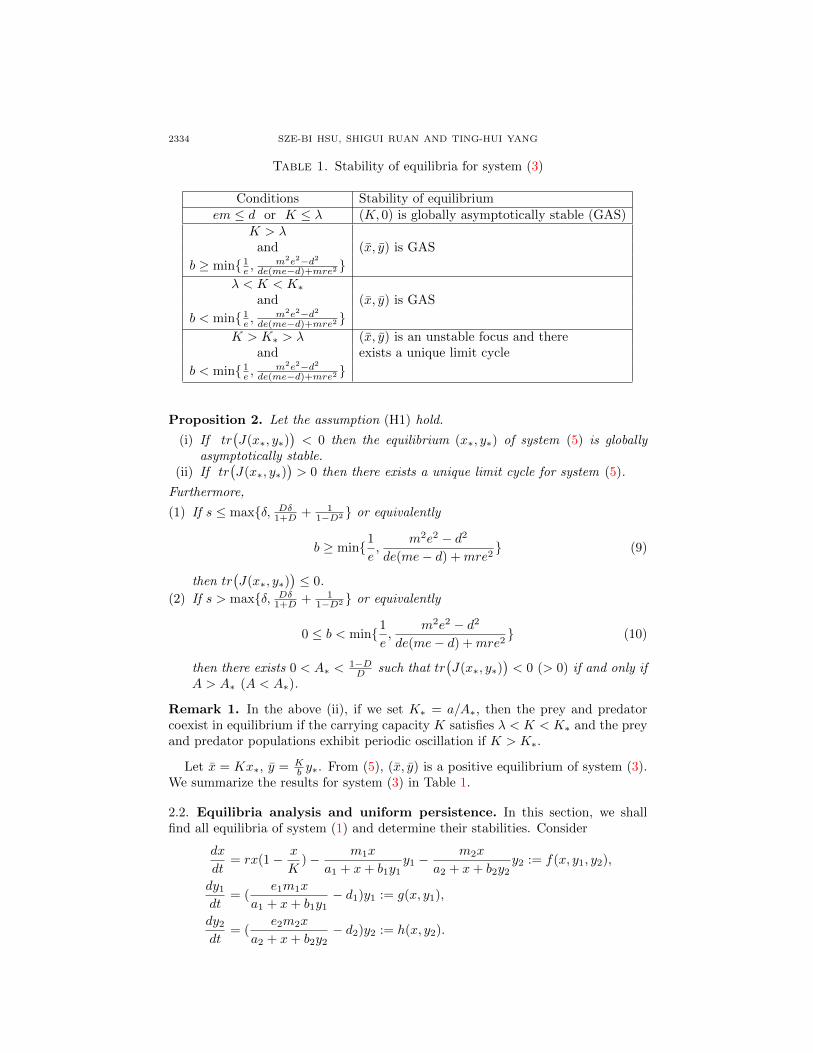
Table 1. Stability of equilibria for system (3)
Conditions Stability of equilibriumem ≤ d or K ≤ λ (K, 0) is globally asymptotically stable (GAS)
K > λ(x, y) is GASand
b ≥ min{ 1e ,
m2e2−d2de(me−d)+mre2 }
λ < K < K∗(x, y) is GASand
b < min{ 1e ,
m2e2−d2de(me−d)+mre2 }
K > K∗ > λ (x, y) is an unstable focus and thereand exists a unique limit cycle
b < min{ 1e ,
m2e2−d2de(me−d)+mre2 }
Proposition 2. Let the assumption (H1) hold.
(i) If tr(J(x∗, y∗)
)< 0 then the equilibrium (x∗, y∗) of system (5) is globally
asymptotically stable.(ii) If tr
(J(x∗, y∗)
)> 0 then there exists a unique limit cycle for system (5).
Furthermore,
(1) If s ≤ max{δ, Dδ1+D + 1
1−D2 } or equivalently
b ≥ min{1
e,
m2e2 − d2
de(me− d) +mre2} (9)
then tr(J(x∗, y∗)
)≤ 0.
(2) If s > max{δ, Dδ1+D + 1
1−D2 } or equivalently
0 ≤ b < min{1
e,
m2e2 − d2
de(me− d) +mre2} (10)
then there exists 0 < A∗ <1−DD such that tr
(J(x∗, y∗)
)< 0 (> 0) if and only if
A > A∗ (A < A∗).
Remark 1. In the above (ii), if we set K∗ = a/A∗, then the prey and predatorcoexist in equilibrium if the carrying capacity K satisfies λ < K < K∗ and the preyand predator populations exhibit periodic oscillation if K > K∗.
Let x = Kx∗, y = Kb y∗. From (5), (x, y) is a positive equilibrium of system (3).
We summarize the results for system (3) in Table 1.
2.2. Equilibria analysis and uniform persistence. In this section, we shallfind all equilibria of system (1) and determine their stabilities. Consider
dx
dt= rx(1− x
K)− m1x
a1 + x+ b1y1y1 −
m2x
a2 + x+ b2y2y2 := f(x, y1, y2),
dy1
dt= (
e1m1x
a1 + x+ b1y1− d1)y1 := g(x, y1),
dy2
dt= (
e2m2x
a2 + x+ b2y2− d2)y2 := h(x, y2).

TWO-CONSUMERS-ONE-RESOURCE COMPETING SYSTEMS 2335
Then the Jacobian matrix of system (1) takes the form
J(x, y1, y2) =
fx fy1 fy2gx gy1 0hx 0 hy2
(11)
where
fx = r(1− x
K)− m1y1
a1 + x+ b1y1− m2y2
a2 + x+ b2y2+
x(− r
K+
m1y1
(a1 + x+ b1y1)2+
m2y2
(a2 + x+ b2y2)2),
fy1 = − m1x(a1 + x)
(a1 + x+ b1y1)2,
fy2 = − m2x(a2 + x)
(a2 + x+ b2y2)2,
gx =e1m1y1(a1 + b1y1)
(a1 + x+ b1y1)2,
gy1 =e1m1x
a1 + x+ b1y1− d1 −
b1e1m1xy1
(a1 + x+ b1y1)2=
e1m1x(a1 + x)
(a1 + x+ b1y1)2− d1,
hx =e2m2y2(a2 + b2y2)
(a2 + x+ b2y2)2,
hy2 =e2m2x
a2 + x+ b2y2− d2 −
b2e2m2xy2
(a2 + x+ b2y2)2=
e2m2x(a2 + x)
(a2 + x+ b2y2)2− d2.
We now consider the equilibria and periodic solutions on the boundary.(a) E0 = (0, 0, 0). The trivial equilibrium E0 always exists and is a saddle witha two-dimensional stable manifold {(x, y, z) : x = 0, y1 > 0, y2 > 0} and a one-dimensional unstable manifold {(x, y, z) : y1 = 0, y2 = 0}.(b) EK = (K, 0, 0). The semi-trivial equilibrium EK always exists. The Jacobianmatrix at EK is given by
J(EK) =
−r ∗ ∗0 e1m1K
a1+K − d1 0
0 0 e2m2Ka2+K − d2
.Then EK is asymptotically stable if
e1m1K
a1 +K− d1 < 0 and
e2m2K
a2 +K− d2 < 0 .
We note that eimiKai+K
− di < 0 if and only if
eimi ≤ di or K < λi =ai
( eimi
di)− 1
,
where λi is the break-even density for the i-th predator where there is no intraspe-cific competition within the population of the i-th predator. If K > λ1 and K > λ2
then EK is a saddle with a one-dimensional stable manifold {(x, y1, y2) : x > 0, y1 =y2 = 0}.
Actually, we can verify the global asymptotical stability of EK under a weakercondition in the following lemma.
Lemma 2.1. If eimi ≤ di then lim supt→∞ yi(t) = 0 for i = 1, 2.

2336 SZE-BI HSU, SHIGUI RUAN AND TING-HUI YANG
Proof. We only prove the case of i = 1. By the first equation of (1), we know thatlim supt→∞ x(t) ≤ K. So we assume x(t) ≤ K for t large enough. It is easy to seethat
e1m1K ≤ d1K < d1(a1 +K).
Let µ = d1− e1m1Ka1+K > 0. According to the monotonicity of the function e1m1x
a+x withrespect to x, we have
y1
y1=
e1m1x
a1 + x+ by1− d1 <
e1m1x
a1 + x− d1 ≤
e1m1K
a1 +K− d1 = −µ.
This implies that lim supt→∞ y1(t) = 0. We complete the proof.
From now on we always assume that
(H2): e1m1 > d1 and e2m2 > d2.
Hence eimiKai+K
− di < 0 if and only if K < λi if (H2) holds.
(c) E1 = (x1, y1, 0). The semi-trivial equilibrium E1 is a boundary equilibrium onthe (x, y1)-plane, where x1, y1 are obtained by restricting to the system of the firstpredator y1 and the prey x. The Jacobian matrix at E1 is given by
J(E1) =
x1(− rK + m1y1
(a1+x1+b1y1)2 ) − m1x1(a1+x1)(a1+x1+b1y1)2 − m2x1
a2+x1e1m1y1(a1+b1y1)(a1+x1+b1y1)2 − b1e1m1x1y1
(a1+x1+b1y1)2 0
0 0 e2m2x1
a2+x1− d2
.We note that the top left 2 × 2 submatrix is exactly the Jacobian matrix J in (8)for the subsystem (3) at the equilibrium (x∗, y∗), where a, b, e, m, d are replaced bya1, b1, e1, m1, d1 (The conditions are presented in Table 1). And e2m2x1
a2+x1− d2 < 0
if and only if x1 < λ2 under the assumption (H2). There are four cases for thestability of E1.
Case A1:: The equilibrium E1 is asymptotically stable in R3 if (x1, y1) is anasymptotically stable equilibrium for system (3) with a, b, e, m, d replaced bya1, b1, e1, m1, d1 (The conditions are presented in Table 1) and e2m2x1
a2+x1−d2 <
0.Case A2:: If (x1, y1) is an asymptotically stable equilibrium for system (3) andx1 > λ2, then E1 is a saddle with a one-dimensional unstable manifold Wu
1
and a two-dimensional stable manifold on the (x, y1) plane.Case A3:: If (x1, y1) is an unstable focus for system (3) and x1 < λ2, then E1 is
a saddle with a one-dimensional stable manifold W s1 and a unique limit cycle
Γ1 on the (x, y1) plane.Case A4:: If (x1, y1) is an unstable focus for system (3) and x1 > λ2, then E1
is a repeller.
We summarize the results on local stability of the boundary equilibrium E1 forsystem (1) in Table 2.(d) E2 = (x2, 0, y2). Similar to the above case (c), the Jacobian matrix at E2 isgiven by
J(E1) =
x2(− rK + m2y2
(a2+x2+b2y2)2 ) − m1x2
a1+x2− m2x2(a2+x2)
(a2+x2+b2y2)2
0 e1m1x2
a1+x2− d1 0
e2m2y2(a2+b2y2)(a2+x2+b2y2)2 0 − b2e2m2x2y2
(a2+x2+b2y2)2
.We note that the 2 × 2 submatrix gotten by deleting the second row and secondcolumn of above matrix is exactly the Jacobian matrix J in (8) for the subsystem

TWO-CONSUMERS-ONE-RESOURCE COMPETING SYSTEMS 2337
Table 2. Stability of equilibrium E1 for system (1)
Conditions Stability of equilibrium E1
K > λ1
and x1 < λ2 E1 is GAS
b1 ≥ min{ 1e1,
m21e
21−d
21
d1e1(m1e1−d1)+m1re21} (x1 > λ2) (E1 is a saddle with a one-dimen-
λ1 < K < K∗ sional unstable manifold Wu1 and
and a two-dimensional stable manifold
b1 < min{ 1e1,
m21e
21−d
21
d1e1(m1e1−d1)+m1re21} on the (x, y1) plane.)
K > K∗ > λ1 x1 < λ2 E1 is an unstable focus and there
and exists a unique limit cycle
b1 < min{ 1e1,
m21e
21−d
21
d1e1(m1e1−d1)+m1re21} (x1 > λ2) (E1 is a repeller)
Table 3. Stability of equilibrium E2 for system (1)
Conditions Stability of equilibrium E2
K > λ2
and x2 < λ1 E2 is GAS
b2 ≥ min{ 1e2,
m22e
22−d
22
d2e2(m2e2−d2)+m2re22} (x2 > λ1) (E2 is a saddle with a one-dimen-
λ2 < K < K∗ sional unstable manifold Wu2 and
and a two-dimensional stable manifold
b2 < min{ 1e2,
m22e
22−d
22
d2e2(m2e2−d2)+m2re22} on the (x, y2) plane.)
K > K∗ > λ2 x2 < λ1 E2 is an unstable focus and there
and exists a unique limit cycle
b1 < min{ 1e1,
m21e
21−d
21
d1e1(m1e1−d1)+m1re21} (x2 > λ1) (E2 is a repeller)
(3) at the equilibrium (x∗, y∗) where a, b, e, m, d are replaced by a2, b2, e2, m2, d2.We have four cases:
Case B1:: The equilibrium E2 is asymptotically stable in R3 if (x2, y2) is anasymptotically stable equilibrium for system (3) with a, b, e, m, d replacedby a2, b2, e2, m2, d2 and x2 < λ1.
Case B2:: If (x2, y2) is an asymptotically stable equilibrium for system (3) andx2 > λ1, then E2 is a saddle with a one-dimensional unstable manifold Wu
2
and a two-dimensional stable manifold on the (x, y2) planeCase B3:: If (x2, y2) is an unstable focus for the system (3) and x2 < λ1, thenE2 is a saddle with a one-dimensional stable manifold W s
2 and a unique limitcycle Γ2 on the (x, y2) plane.
Case B4:: If (x2, y2) is an unstable focus for system (3) and x2 > λ1, then E2
is a repeller.
Similarly, we summarize the results on local stability of the boundary equilibriumE2 for system (1) in Table 3.(e) EΓ1
= (φ1, ψ1, 0). If the condition in Proposition 2 (ii) is satisfied, then theequilibrium E = (x1, y1) on the (x, y1) plane is unstable and there is a uniquestable limit cycle Γ1 on the (x, y1) plane, denoted by (φ1(t), ψ1(t)). Consequently,EΓ1 = (φ1, ψ1, 0) is a boundary periodic solution for system (1). Since EΓ1 is stable

2338 SZE-BI HSU, SHIGUI RUAN AND TING-HUI YANG
restricted to the (x, y1) plane, we only need to discuss its stability in the y2-axisdirection.
The stability of EΓ1is determined by the Floquet multipliers of the variational
system
Φ(t) = J(φ1, ψ1, 0)Φ(t), Φ(0) = I (12)
where J(x, y1, y2) is defined in (11) and I is the 3×3 identity matrix. Let ω1 be theperiod of the periodic solution (φ1, ψ1). Then the Floquet multiplier correspondingto the y2-direction is given by
exp[1
ω1
∫ ω1
0
(m2e2φ1(t)
a2 + φ1(t)− d2) dt].
Thus EΓ1 is stable if
d2 >
∫ ω1
0
m2e2φ1(t)
a2 + φ1(t)dt (13)
and unstable if
d2 <
∫ ω1
0
m2e2φ1(t)
a2 + φ1(t)dt . (14)
(f) Similarly, if the boundary periodic solution EΓ2= (φ2(t), 0, ψ2(t)) with period
ω2 exists then it is stable if
d1 >
∫ ω2
0
m1e1φ2(t)
a1 + φ2(t)dt (15)
and unstable if
d1 <
∫ ω2
0
m1e1φ2(t)
a1 + φ2(t)dt . (16)
We now have the following results on the uniform persistence of system (1). (Bulteret. al [4], Butler and Waltman [3], Freedman et. al [9], Smith and Thieme [22]).
Theorem 2.2. Assume one of the following cases holds:
(i) Let Case A2 and Case B2 holds, i.e., E1 and E2 are unstable in the y2-axisand the y1-axis direction, respectively.
(ii) Let Case A2, Case B4 and (16) hold, i.e., E1 and EΓ2are unstable in the
y2-axis and the y1-axis direction, respectively.(iii) Let Case B2, Case A4 and (14) hold, i.e., E2 and EΓ1 are unstable in the
y1-axis and the y2-axis direction, respectively.(iv) Let Case A4, (14), Case B4 and (16) hold, i.e., EΓ1
and EΓ2are unstable
in the y2-axis and the y1-axis direction, respectively.
Then system (1) is uniformly persistent.
(g) Ec = (xc, y1c, y2c). From the 2nd and 3rd equations of (1), xc, y1c, y2c satisfy
eimix
ai + x+ biyi= di (17)
for i = 1, 2 or
y1c = M1(xc − λ1) > 0, y2c = M2(xc − λ2) > 0 (18)
where we use the notations M1 = e1m1−d1d1b1
and M2 = e2m2−d2d2b2
for simplifying.Assume that
(H3): 0 < λ1 < λ2 < K.

TWO-CONSUMERS-ONE-RESOURCE COMPETING SYSTEMS 2339
From the first equation of (1), xc satisfies the equation
rx(1− x
K)− d1
e1M1(x− λ1)− d2
e2M2(x− λ2) = 0.
Let
F (x) = rx(1− x
K)− d1
e1M1(x− λ1)− d2
e2M2(x− λ2).
Then F (K) < 0, F (0) > 0, F (λ1) > 0, and
F (λ2) = rλ2(1− λ2
K)− d1
e1M1(λ2 − λ1).
Hence if
F (λ2) > 0 (19)
then Ec = (xc, y1c, y2c) exists and is unique. If
F (λ2) < 0 (20)
then Ec does not exist. Rewrite
F (x) = (− r
K)x2 + x
(r − d1
e1M1 −
d2
e2M2
)+(d1
e1M1λ1 +
d2
e2M2λ2
).
Then xc is the unique positive root of F (x) = 0,
xc =K(B +
√B2 + 4rC/K)
2r(21)
where B = r − d1e1M1 − d2
e2M2 and C = d1
e1M1λ1 + d2
e2M2λ2. The condition (19) for
the existence of Ec is equivalent to
K > λ2
(1− d1
re1λ2M1(λ2 − λ1)
)−1= K > 0 (22)
or xc > λ2. We note that in (22) we need
r >d1
e1M1(1− λ1
λ2) (23)
The Jacobian matrix of the system (1) at Ec takes the form
J(Ec) =
f∗x f∗y1 f∗y2g∗x g∗y1 0h∗x 0 h∗y2
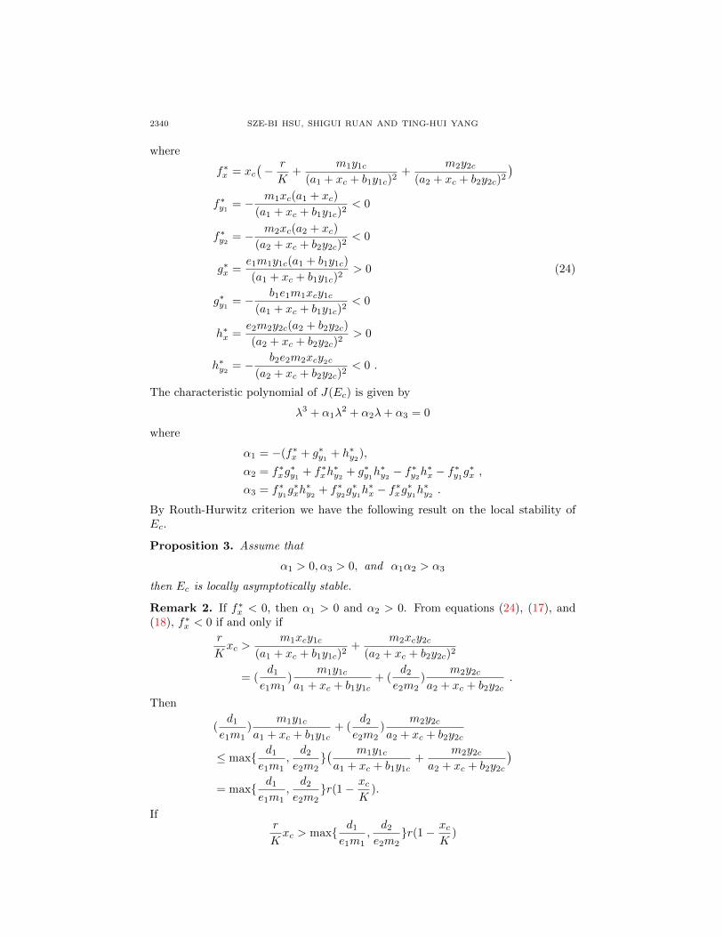
2340 SZE-BI HSU, SHIGUI RUAN AND TING-HUI YANG
where
f∗x = xc(− r
K+
m1y1c
(a1 + xc + b1y1c)2+
m2y2c
(a2 + xc + b2y2c)2
)f∗y1 = − m1xc(a1 + xc)
(a1 + xc + b1y1c)2< 0
f∗y2 = − m2xc(a2 + xc)
(a2 + xc + b2y2c)2< 0
g∗x =e1m1y1c(a1 + b1y1c)
(a1 + xc + b1y1c)2> 0 (24)
g∗y1 = − b1e1m1xcy1c
(a1 + xc + b1y1c)2< 0
h∗x =e2m2y2c(a2 + b2y2c)
(a2 + xc + b2y2c)2> 0
h∗y2 = − b2e2m2xcy2c
(a2 + xc + b2y2c)2< 0 .
The characteristic polynomial of J(Ec) is given by
λ3 + α1λ2 + α2λ+ α3 = 0
where
α1 = −(f∗x + g∗y1 + h∗y2),
α2 = f∗xg∗y1 + f∗xh
∗y2 + g∗y1h
∗y2 − f
∗y2h∗x − f∗y1g
∗x ,
α3 = f∗y1g∗xh∗y2 + f∗y2g
∗y1h∗x − f∗xg∗y1h
∗y2 .
By Routh-Hurwitz criterion we have the following result on the local stability ofEc.
Proposition 3. Assume that
α1 > 0, α3 > 0, and α1α2 > α3
then Ec is locally asymptotically stable.
Remark 2. If f∗x < 0, then α1 > 0 and α2 > 0. From equations (24), (17), and(18), f∗x < 0 if and only if
r
Kxc >
m1xcy1c
(a1 + xc + b1y1c)2+
m2xcy2c
(a2 + xc + b2y2c)2
= (d1
e1m1)
m1y1c
a1 + xc + b1y1c+ (
d2
e2m2)
m2y2c
a2 + xc + b2y2c.
Then
(d1
e1m1)
m1y1c
a1 + xc + b1y1c+ (
d2
e2m2)
m2y2c
a2 + xc + b2y2c
≤ max{ d1
e1m1,d2
e2m2}( m1y1c
a1 + xc + b1y1c+
m2y2c
a2 + xc + b2y2c
)= max{ d1
e1m1,d2
e2m2}r(1− xc
K).
Ifr
Kxc > max{ d1
e1m1,d2
e2m2}r(1− xc
K)

TWO-CONSUMERS-ONE-RESOURCE COMPETING SYSTEMS 2341
or equivalentM
1 + MK < xc < K,
where M = max{ d1e1m1
, d2e2m2}, then f∗x < 0.
2.3. Hopf bifurcation. In this section, we will verify that the Hopf bifurcationindeed occurs. It is obvious that if b1e1 ≥ 1 and b2e2 ≥ 1, then α1 and α3 arepositive for all K > 0 from the expressions of α1 and α3
α1 = −(f∗x + g∗y1 + h∗y2),
=rxcK− m1 xc y1c
(b1 y1c + xc + a1)2 −
m2 xc y2c
(b2 y2c + xc + a2)2 +
b1 e1m1 xc y1c
(b1 y1c + xc + a1)2 +
b2 e2m2 xc y2c
(b2 y2c + xc + a2)2 ,
α3 = f∗y1g∗xh∗y2 + f∗y2g
∗y1h∗x − f∗xg∗y1h
∗y2
=b2 e1 e2m1
2m2 xc2 (xc + a1) y1c (b1 y1c + a1) y2c
(b1 y1c + xc + a1)4
(b2 y2c + xc + a2)2 +
b1 e1 e2m1m22 xc
2 (xc + a2) y1c y2c (b2 y2c + a2)
(b1 y1c + xc + a1)2
(b2 y2c + xc + a2)4 +
b1b2e1e2m1m2xc2y1cy2c
(r xc
K −m2 xc y2c
(b2 y2c+xc+a2)2− m1 xc y1c
(b1 y1c+xc+a1)2
)(b1 y1c + xc + a1)
2(b2 y2c + xc + a2)
2
=a1b2 e1 e2m1
2m2 xc2 y1c y2c
(b1 y1c + xc + a1)3
(b2 y2c + xc + a2)2 +
a2b1 e1 e2m1m22 xc
2 y1c y2c
(b1 y1c + xc + a1)2
(b2 y2c + xc + a2)3
+rb1b2e1e2m1m2xc
3y1cy2c
K (b1 y1c + xc + a1)2
(b2 y2c + xc + a2)2 > 0 .
Hence, by Proposition 3, the positive equilibrium Ec will lose its stability if α1α2−α3 ≤ 0. We take K as the bifurcation parameter. It is easy to see that xc, y1c, andy2c are functions of K by the equations (21) and (18). The expression of α1α2−α3
has the form,
α1α2 − α3 = −(f∗x + g∗y1 + h∗y2)(f∗xg∗y1 + f∗xh
∗y2 + g∗y1h
∗y2 − f
∗y2h∗x − f∗y1g
∗x)−
(f∗y1g∗xh∗y2 + f∗y2g
∗y1h∗x − f∗xg∗y1h
∗y2)
= −(f∗x)2gy1 − (f∗x)2hy2 − (g∗y1)2hy2 + f∗y1g∗xg∗y1 − g
∗y1(h∗y2)2 + f∗y2h
∗xh∗y2+
f∗x(f∗y2h
∗x + f∗y1g
∗x − (g∗y1)2 − 2g∗y1h
∗y2 − (h∗y2)2
).
In the last formula, we have two classes
−(f∗x)2gy1 − (f∗x)2hy2 − (g∗y1)2hy2 + f∗y1g∗xg∗y1 − g
∗y1(h∗y2)2 + f∗y2h
∗xh∗y2
andf∗x(f∗y2h
∗x + f∗y1g
∗x − (g∗y1)2 − 2g∗y1h
∗y2 − (h∗y2)2
).
All terms of the first class are positive and all term of another one are negativeexcept for the function f∗x . So we should clarify the behavior of f∗x as a function ofK.
By the representation of xc, (21), it is easy to see that if B = r − d1e1M1 −
d2e2M2 > 0 then limK→0+ xc(K) = 0, limK→0+ xc(K)/K > 0, limK→∞ xc(K) =∞,
and limK→∞ xc(K)/K = B/r > 0. These implies limK→0+ f∗x(K) < 0. But
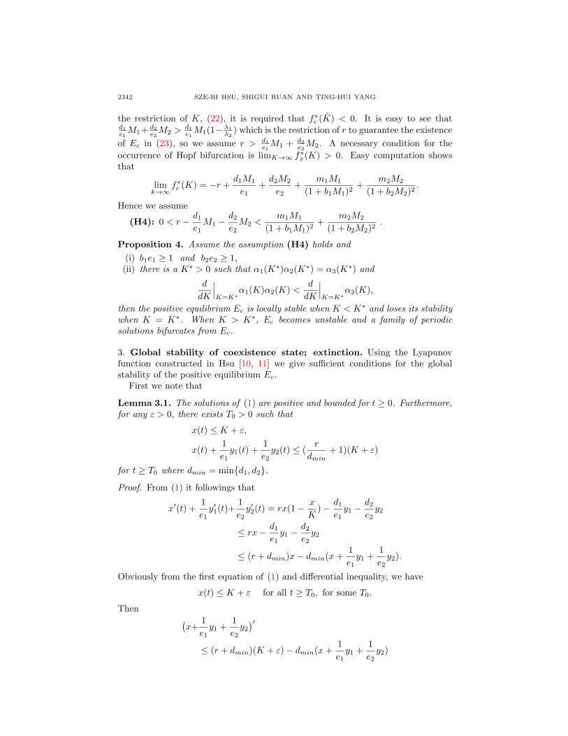
2342 SZE-BI HSU, SHIGUI RUAN AND TING-HUI YANG
the restriction of K, (22), it is required that f∗c (K) < 0. It is easy to see thatd1e1M1+ d2
e2M2 >
d1e1M1(1− λ1
λ2) which is the restriction of r to guarantee the existence
of Ec in (23), so we assume r > d1e1M1 + d2
e2M2. A necessary condition for the
occurrence of Hopf bifurcation is limK→∞ f∗x(K) > 0. Easy computation showsthat
limk→∞
f∗c (K) = −r +d1M1
e1+d2M2
e2+
m1M1
(1 + b1M1)2+
m2M2
(1 + b2M2)2.
Hence we assume
(H4): 0 < r − d1
e1M1 −
d2
e2M2 <
m1M1
(1 + b1M1)2+
m2M2
(1 + b2M2)2.
Proposition 4. Assume the assumption (H4) holds and
(i) b1e1 ≥ 1 and b2e2 ≥ 1,(ii) there is a K∗ > 0 such that α1(K∗)α2(K∗) = α3(K∗) and
d
dK
∣∣∣K=K∗
α1(K)α2(K) <d
dK
∣∣∣K=K∗
α3(K),
then the positive equilibrium Ec is locally stable when K < K∗ and loses its stabilitywhen K = K∗. When K > K∗, Ec becomes unstable and a family of periodicsolutions bifurcates from Ec.
3. Global stability of coexistence state; extinction. Using the Lyapunovfunction constructed in Hsu [10, 11] we give sufficient conditions for the globalstability of the positive equilibrium Ec.
First we note that
Lemma 3.1. The solutions of (1) are positive and bounded for t ≥ 0. Furthermore,for any ε > 0, there exists T0 > 0 such that
x(t) ≤ K + ε,
x(t) +1
e1y1(t) +
1
e2y2(t) ≤ (
r
dmin+ 1)(K + ε)
for t ≥ T0 where dmin = min{d1, d2}.
Proof. From (1) it followings that
x′(t) +1
e1y′1(t)+
1
e2y′2(t) = rx(1− x
K)− d1
e1y1 −
d2
e2y2
≤ rx− d1
e1y1 −
d2
e2y2
≤ (r + dmin)x− dmin(x+1
e1y1 +
1
e2y2).
Obviously from the first equation of (1) and differential inequality, we have
x(t) ≤ K + ε for all t ≥ T0, for some T0.
Then (x+
1
e1y1 +
1
e2y2
)′≤ (r + dmin)(K + ε)− dmin(x+
1
e1y1 +
1
e2y2)
TWO-CONSUMERS-ONE-RESOURCE COMPETING SYSTEMS 2343
Then we have
x(t)+1
e1y1(t) +
1
e2y2(t) ≤ (
r
dmin+ 1)(K + ε) for t ≥ T0.
Theorem 3.2. Let the assumption (H3) hold. Assume Ec exists, i.e., (22) and(23) hold. If
K <1
max{1/a1, 1/a2}+ xc (25)
then the positive equilibrium Ec is globally stable.
Proof. Choose a Lyapunov function as follows
V (x, y1, y2) =
∫ x
xc
ξ − xcξ
dξ + α
∫ y1
y1c
ξ − y1c
ξdξ + β
∫ y2
y2c
ξ − y2c
ξdξ ,
where α and β are positive constants to be determined. Along the trajectories ofthe system (1) we have
dV
dt= (x− xc)
(r(1− x
K)− m1y1
a1 + x+ b1y1− m2y2
a2 + x+ b2y2
)+ α(y1 − y1c)
( m1e1x
a1 + x+ b1y1− d1
)+ β(y2 − y2c)
( m2e2x
a2 + x+ b2y2− d2
)= (x− xc)
{− r
K(x− xc)−
( m1y1
a1 + x+ b1y1− m1y1c
a1 + xc + b1y1c
)−( m2y2
a2 + x+ b2y2− m2y2c
a2 + xc + b2y2c
)}+ α(y1 − y1c)
( m1e1x
a1 + x+ b1y1− m1e1xca1 + xc + b1y1c
)+ β(y2 − y2c)
( m2e2x
a2 + x+ b2y2− m2e2xca2 + xc + b2y2c
)= (x− xc)
{− r
K(x− xc)−
m1
((a1 + xc)(y1 − y1c)− y1c(x− xc)
)(a1 + x+ b1y1)(a1 + xc + b1y1c)
−m2
((a2 + xc)(y2 − y2c)− y2c(x− xc)
)(a2 + x+ b2y2)(a2 + xc + b2y2c)
}+ α(y1 − y1c)
m1e1
((a1 + b1y1c)(x− xc)− b1xc(y1 − y1c)
)(a1 + x+ b1y1)(a1 + xc + b1y1c)
+ β(y2 − y2c)m2e2
((a2 + b2y2c)(x− xc)− b2xc(y2 − y2c)
)(a2 + x+ b2y2)(a2 + xc + b2y2c)
.
Choose α = a1+xc
e1(a1+b1y1c) and β = a2+xc
e2(a2+b2y2c) . Therefore,
dV
dt= (x− xc)2
{− r
K+
m1y1c
(a1 + x+ b1y1)(a1 + xc + b1y1c)
+m2y2c
(a2 + x+ b2y1)(a2 + xc + b2y2c)
}− αb1xc(y1 − y1c)
2
(a1 + x+ b1y1)(a1 + xc + b1y1c)− βb2xc(y2 − y2c)
2
(a2 + x+ b2y2)(a2 + xc + b2y2c).

2344 SZE-BI HSU, SHIGUI RUAN AND TING-HUI YANG
The coefficients of (y1−y1c)2 and (y2−y2c)
2 are negative. The coefficient of (x−xc)2
is
− r
K+
m1y1c
(a1 + x+ b1y1)(a1 + xc + b1y1c)+
m2y2c
(a2 + x+ b2y1)(a2 + xc + b2y2c)
≤ − r
K+
m1y1c
a1(a1 + xc + b1y1c)+
m2y2c
a2(a2 + xc + b2y2c)
≤ − r
K+ max{ 1
a1,
1
a2}r(1− xc
K)
= − r
K
(1−max{ 1
a1,
1
a2}(K − xc)
).
If (25) is satisfied, then dV/dt ≤ 0 and dV/dt = 0 if and only if x = xc, y1 = y1c,and y2 = y2c. The largest invariant set of {dV/dt = 0} is {(xc, y1c, y2c)}. There-fore, Lemma 3.1 and LaSalle’s Invariant Principle imply that Ec = (xc, y1c, y2c) isglobally stable. Thus we complete the proof.
Remark 3. Under the assumption (H2) and (22), (23), Ec exists and xc > λ2. Let
K = λ2(1− 1reλ2
me1−d1b1
(λ2 − λ1))−1. If r is sufficient large then
K <1
max{1/a1, 1/a2}+ λ2 <
1
max{1/a1, 1/a2}+ xc .
Thus the condition (25) is feasible when r is sufficiently large.
The following extinction result for system (1) is similar to Lemma 4.3 [12] andTheorem 3.6 [14] of Hsu, Hubbell and Waltman for system (2).
Theorem 3.3. Let the assumption (H3) hold.
(i) If a1 ≥ a2 or(ii) if a1 < a2 but δ1 ≥ δ2 where δi = miei/di, i = 1, 2 or
(iii) if a1 < a2, δ1 < δ2 but K < a2δ1−a1δ2δ2−δ1
then limt→∞ y2(t) = 0 for any b1 > 0 and b2 > 0 sufficiently small.
Proof. Let ξ > 0. Then
ξy′2(t)
y2(t)− y′1(t)
y1(t)= ξ[
e1m1x
a1 + x+ b1y1− d1]− [
e2m2x
a2 + x+ b2y2− d2]
≤ ξ[e1m1x
a1 + x− d1]− [
e2m2x
a2 + x− d2] + [
e2m2x
a2 + x− e2m2x
a2 + x+ b2y2] (26)
Let
Pξ(x) =ξ[e1m1x
a1 + x− d1]− [
e2m2x
a2 + x− d2]
=ξ(e1m1 − d1)(x− λ1)
a1 + x− (e2m2 − d2)
x− λ2
a2 + x.
Under the assumption (H3) and (i) or (ii), from Lemma 4.3 [12], we can chooseξ∗ > 0 such that
Pξ∗(x) ≤ −ζ < 0 for all 0 ≤ x ≤ K + ε, for some ζ > 0.

TWO-CONSUMERS-ONE-RESOURCE COMPETING SYSTEMS 2345
Consider the third term in (26)
0 <e2m2x
a2 + x− e2m2x
a2 + x+ b2y2
=e2m2xb2y2
(a2 + x)(a2 + x+ b2y2)
=b2e2m2x
a2 + x
y2
a2 + x+ b2y2
<b2e2m2(K + ε)
a2 + (K + ε)· 1
a2(y2)max < b2∆
where ∆ =e22m2(K+ε)2
a2(a2+K+ε) ( rdmin
+ 1). We note that from the bound in Lemma 3.1 ∆
is independent of b2. Hence for b2 > 0 sufficiently small satisfying b2∆− ζ < 0, wehave
ξ∗y′2(t)
y2(t)− y′1(t)
y1(t)≤ b2∆− ζ < 0.
Then y2(t)→ 0 as t→∞.If (H3) and (iii) hold then
y′2(t)
d2y2(t)− y′1(t)
d1y1(t)=
δ1x
a1 + x+ b1y1− δ2x
a2 + x+ b2y2
≤ δ1x
a1 + x− δ2x
a2 + x+( δ2x
a2 + x− δ2x
a2 + x+ b2y2
).
Let P (x) = δ1xa1+x −
δ2xa2+x . Then from (iii) and the proof of Theorem 3.6 in [14],
P (x) ≤ −ζ < 0, for all 0 ≤ x ≤ K + ε for some ζ > 0.
Similarly,
0 <δ2x
a2 + x− δ2x
a2 + x+ b2y2< b2∆
where ∆ = δ2e2(K+ε)2
a2(a2+K+ε)
(r
dmin+ 1). Then the similar arguments as above yields
limt→∞
y2(t) = 0.
This completes the proof.
4. Competition of two identical species with different interference effects.In this section we consider two identical predators competing for a shared prey withdifference in predator interference effects b1 6= b2. The equations are the following:
x′ = rx(1− x
K)− mxy1
a+ x+ b1y1− mxy2
a+ x+ b2y2,
y1′ = (
emx
a+ x+ b1y1− d)y1 , (27)
y2′ = (
emx
a+ x+ b2y2− d)y2 ,
with initial conditions x(0) > 0, y1(0) > 0, y2(0) > 0. Let
K > λ1 = λ2 = a/(em
d− 1). (28)

2346 SZE-BI HSU, SHIGUI RUAN AND TING-HUI YANG
Assume b2 > b1. Then
y1′ = (
emx
a+ x+ b1y1− d)y1
> (emx
a+ x+ b2y1− d)y1 .
Thus, if y1(0) ≥ y2(0) then y1(t) > y2(t) for all t ≥ 0. If y1(0) < y2(0) then eitherthere exists t0 > 0 such that y1(t0) = y2(t0) or y1(t) < y2(t) for all t ≥ 0. Ify1(t0) = y2(t0) then
y1(t) > y2(t) for all t ≥ t0. (29)
If y1(t) < y2(t) for all t ≥ 0 then
y1′
y1=
emx
a+ x+ b1y1− d > emx
a+ x+ b2y2− d =
y2′
y2.
We have
y1(t)
y1(0)>y2(t)
y2(0). (30)
Thus, we have either y1(t0) > y2(t0) for some t0 > 0 or y2(0)y1(t) > y1(0)y2(t) forall t ≥ 0. If y1(t) → 0 as t → ∞ then y2(t) → 0 as t → ∞. Hence we obtain acontradiction to the assumption (28). Hence
lim supt→∞
y1(t) > 0. (31)
On the other hand, assume y2(t) → 0 as t → ∞. Let Case A1 hold. Thenx(t)→ x1 and y1(t)→ y1 as t→∞ and emx1
a+x1+b1y1= d. Thus
emx1
a+ x1− d > 0 . (32)
Let Case A3 hold. Then (x(t), y1(t))→ (φ1(t), ψ1(t)) as t→∞ and∫ ω1
0
( emφ1(t)
a+ φ1(t) + b1ψ1(t)− d)dt = 0.
Hence ∫ ω1
0
( emφ1(t)
a+ φ1(t)− d)dt > 0 . (33)
However, (32) and (33) imply that E1 and EΓ1are unstable in the y2-axis direction
respectively. Thus the assumption y2(t) → 0 as t → ∞ leads to a contradiction.Hence we have the following results.
Theorem 4.1. For system (27), if (28) holds then lim supt→∞ y1(t) > 0 andlim supt→∞ y2(t) > 0.
5. Relaxation oscillations. Consider system (1) with a large prey intrinsic growthrate, i.e., r � 1. Let ε = 1/r. Then 0 < ε� 1, With the scaling:
x→ x/K, a1 → a1/K, a2 → a2/K, y1 = y1/(Kr), y2 = y2/(Kr),
TWO-CONSUMERS-ONE-RESOURCE COMPETING SYSTEMS 2347
system (1) becomes
εx′ = x(1− x)− m1xy1
a1 + x+ ( b1ε )y1
− m2xy2
a2 + x+ ( b2ε )y2
y1′ = (
e1m1x
a1 + x+ ( b1ε )y1
− d1)y1 (34)
y2′ = (
e2m2x
a2 + x+ ( b2ε )y2
− d2)y2
Assume b1 = b1(ε), b2 = b2(ε) such that
bi(ε) = O(ε1+µi) as ε→ 0 (35)
for some µi > 0, i = 1, 2. Under the assumption (35) we apply the geometricsingular perturbation method as in Liu, Xiao, and Yi [19] to prove the existence ofperiodic solutions.
Setting ε = 0 in (34) results in the so-called limiting slow system
xF (x, y1, y2) = x(1− x− m1y1
a1 + x− m2y2
a2 + x
),
y1′ = (
e1m1x
a1 + x− d1)y1, (36)
y2′ = (
e2m2x
a2 + x− d2)y2,
which is generally defined on the slow manifold S0 = {(x, y1, y2) : xF (x, y1, y2) =0, x ≥ 0, y1 ≥ 0, y2 ≥ 0}. Orbits or parts of orbits of the system (36) on S0 arecalled the slow orbits of system (34) and the variables y1, y2 are called slow variables.For system (36), the slow manifold S0 consists of two portions S1 and S2, whereS1 = {(x, y, z) ∈ S0 : x = 0}, S2 = {(x, y1, y2) : F (x, y1, y2) = 0}.
In term of the fast time scale τ = t/ε, system (34) becomes
dy1
dτ= εy1(
e1m1x
a1 + x+ ( b1ε )y1
− d1),
dy2
dτ= εy2(
e2m2x
a2 + x+ ( b2ε )y2
− d2), (37)
dx
dτ= x
(1− x− m1y1
a1 + x+ ( b1ε )y1
− m2y2
a2 + x+ ( b2ε )y2
).
The system (38) is referred to as the fast system. Its limit, the limiting fast system,is obtained by setting ε = 0:
dy1
dτ= 0,
dy2
dτ= 0,
dx
dτ= xF (x, y1, y2). (38)
The orbits of system (38) are parallel to the x-axis and their directions are charac-terized by the sign of xF (x, y1, y2). We refer to these orbits as fast orbits of system(34) and the variable x is the fast variable.
A continuous and piecewise smooth curve is said to be a limiting orbit of system(34) if it is the union of a finitely many fast and slow orbits with compatible ori-entations. A limiting orbit is called a limiting periodic orbit if it is a simple closedcurve and contains no equilibrium of system (34). A periodic orbit of system (34)is called a relaxation oscillation if its limiting as ε → 0 is a limiting periodic orbitconsisting of both fast and slow orbits.

2348 SZE-BI HSU, SHIGUI RUAN AND TING-HUI YANG
Table 4. Parameter Values in the General Case.
r = 2.0 a1 = 3 b1 = 0.6 d1 = 0.4 e1 = 0.6 m1 = 1.5K = ∗ a2 = 6 b2 = 2.0 d2 = 0.45 e2 = 0.7 m2 = 1.5
Table 5. Parameter Values for the Case with Interference.
r = 20 · ln 2 a1 = 200 d1 = ln 2/2 e1 = 0.1 m1 = 10 · ln 2K = 1100 a2 = 500 d2 = ln 2 e2 = 1.4 m2 = 2 · ln 2
.
In the following theorem, we first prove that under the assumption (35) there isno positive equilibrium for system (34). Then following the methods in Liu, Xiao,and Yi [19] we construct a limiting periodic orbit consisting of both fast and sloworbits. By the theorem of geometric singular perturbation method, there exists astable relaxation oscillation.
Theorem 5.1. Let (H3) and (35) hold. Assume that the relaxation cycle Γε1 on the(x, y1)-plane is unstable in the y2-axis direction and the relaxation cycle Γε2 on the(x, y2)-plane is unstable in the y1-axis direction. Then there is at least one stablerelaxation oscillation in the positive octant of R3.
Proof. If Eεc = (xεc, yε1c, y
ε2c) exists then from (18) and (35), yε1c → ∞ as ε → 0.
Thus the equilibrium Eεc is not on the surface S0 and the limiting periodic orbitdoes not contain Eεc . From Theorem 3.4 in [19], there exists a stable relaxationoscillation in the positive octant of R3. We complete the proof.
6. Numerical simulations. Choose the values of parameters as in Table 4 andcalculate the values λ1 = a1d1
e1m1−d1 = 2.4 and λ2 = a2d2e2m2−d2 = 4.5. Now, using K
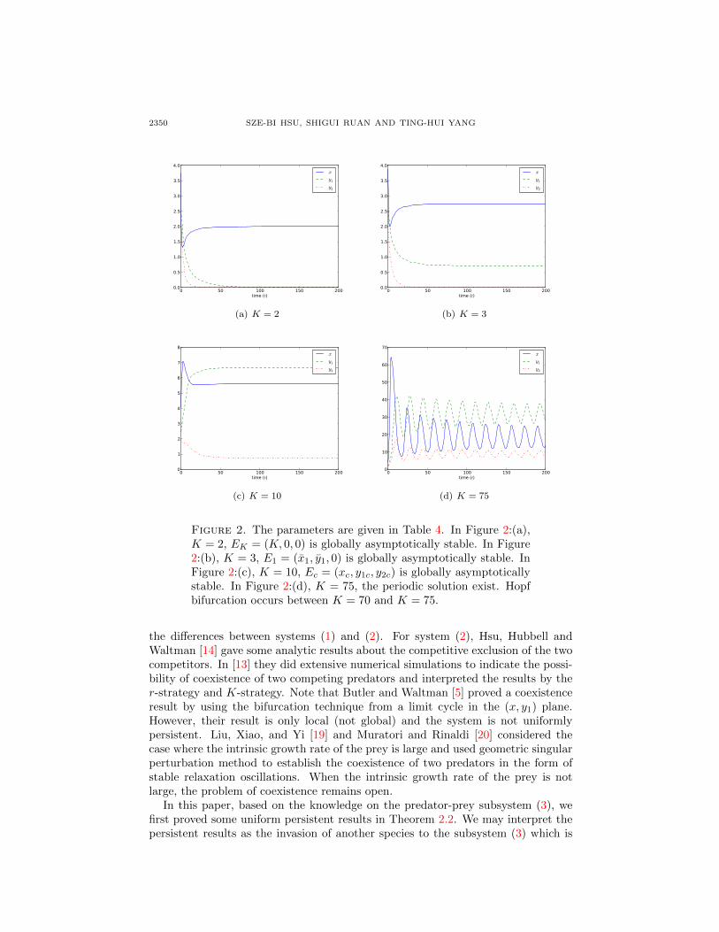
(the carrying capacity of the resource) as a bifurcation parameter, increase K from4.5 to 80 and calculate f∗x(K) as a function of K in (24). We can see that f∗x ismonotonically increasing from negative to positive (see the first graph of Figure 1).The values of functions α1, α3, and α1α2−α3 are also calculated (see the 2nd - 4thgraphs of Figure 1). The dynamics of solutions with respect to the capacity K areillustrated in Figure 2:(a)-(d).
(i) 0 < K = 2 < λ1. The semi-trivial equilibrium EK is globally asymptoticallystable, (see Figure 2:(a))
(ii) λ1 < K = 3 < λ2. The semi-trivial equilibrium E1 is globally asymptoticallystable, (see Figure 2:(b))
(iii) λ2 < K = 10. The solution converges to the positive equilibrium Ec as t→∞.We can see that the positive equilibrium is asymptotically stable, (see Figure2:(c))
(iv) K = 75. The positive equilibrium Ec loses its stability and a periodic solutionbifurcates from it. (see Figure 2:(d))
Next, we do some numerical simulations of system (1) with interference effects,i.e., b1 6= 0 and b2 6= 0. In order to compare the differences of solutions of system(1) with or without interference effects, we choose the same parameters as thosein Fig. 3 of [13] in Table 5. We plot limit cycles of the population of predator 1against that of predator 2 in Figure 3. Figure 3:(a) is for b1 = 0, b2 = 0, (b) is forb1 = 0, b2 = 1, and (c) is for b1 = 1, b2 = 0. All above three limit cycles are plottedin a graph showed in (d). With the same parameters, we compute the numerical

TWO-CONSUMERS-ONE-RESOURCE COMPETING SYSTEMS 2349
0 10 20 30 40 50 60 70 80−1.5
−1.0
−0.5
0.0
0.5f∗ x
0 10 20 30 40 50 60 70 800.00.20.40.60.81.0
α1
0 10 20 30 40 50 60 70 80−0.02−0.010.000.010.020.030.04
α3
0 10 20 30 40 50 60 70 80K
−0.050.000.050.100.150.200.250.30
α1α2−α
3
Figure 1. The graphs of f∗x(K), α1(K), α3(K) andα1(K)α2(K) − α3(K) in terms of K as K increases from4.5 to 80.
solutions of (1) with various parameters b1 and b2. Figure 3:(e) shows the numericalresults where b1, b2 are varied from 0 to 1 with step-size 0.01 in (e). The whiteregion represents that the solutions are periodic and the black region means thatthe solutions approach a positive equilibrium.
7. Discussion. In this paper we have studied the competition system (1) of twopredators competing for a renewable resource (the prey) with functional responsesof Beddington-DeAngelis Type. In the governing equations (1) the parameters bi(i = 1, 2), measuring the effect of interference, is the intra-specific competitioncoefficient among the population of the ith predator. The purpose of this paperis to determine the outcome of competition for system (1), namely, under whatconditions the competitive exclusion holds and under what conditions coexistenceof two competing species occurs.
In [16, 17], Hwang gave a complete classification for the behavior of the solutionsof the predator-prey system with Beddington-DeAngelis functional response (3).The trajectory of the solution of (3) either converges to a positive equilibrium orapproaches a unique limit cycle (see Table 1). We note that (3) is a subsystem of(1). A complete understanding of the predator-prey system (3) will help us to studythe behavior of the solutions of the competition system (1).
Without the interference effects, that is, bi = 0, i = 1, 2, system (1) reduces tosystem (2), the classical model of two competing predators for a renewable resourcewith Holling-type II functional responses [13, 14]. In this paper we want to explore
2350 SZE-BI HSU, SHIGUI RUAN AND TING-HUI YANG
0 50 100 150 200time (t)
0.0
0.5
1.0
1.5
2.0
2.5
3.0
3.5
4.0x
y1
y2
(a) K = 2
0 50 100 150 200time (t)
0.0
0.5
1.0
1.5
2.0
2.5
3.0
3.5
4.0x
y1
y2
(b) K = 3
0 50 100 150 200time (t)
0
1
2
3
4
5
6
7
8x
y1
y2
(c) K = 10
0 50 100 150 200time (t)
0
10
20
30
40
50
60
70x
y1
y2
(d) K = 75
Figure 2. The parameters are given in Table 4. In Figure 2:(a),K = 2, EK = (K, 0, 0) is globally asymptotically stable. In Figure2:(b), K = 3, E1 = (x1, y1, 0) is globally asymptotically stable. InFigure 2:(c), K = 10, Ec = (xc, y1c, y2c) is globally asymptoticallystable. In Figure 2:(d), K = 75, the periodic solution exist. Hopfbifurcation occurs between K = 70 and K = 75.
the differences between systems (1) and (2). For system (2), Hsu, Hubbell andWaltman [14] gave some analytic results about the competitive exclusion of the twocompetitors. In [13] they did extensive numerical simulations to indicate the possi-bility of coexistence of two competing predators and interpreted the results by ther-strategy and K-strategy. Note that Butler and Waltman [5] proved a coexistenceresult by using the bifurcation technique from a limit cycle in the (x, y1) plane.However, their result is only local (not global) and the system is not uniformlypersistent. Liu, Xiao, and Yi [19] and Muratori and Rinaldi [20] considered thecase where the intrinsic growth rate of the prey is large and used geometric singularperturbation method to establish the coexistence of two predators in the form ofstable relaxation oscillations. When the intrinsic growth rate of the prey is notlarge, the problem of coexistence remains open.
In this paper, based on the knowledge on the predator-prey subsystem (3), wefirst proved some uniform persistent results in Theorem 2.2. We may interpret thepersistent results as the invasion of another species to the subsystem (3) which is

TWO-CONSUMERS-ONE-RESOURCE COMPETING SYSTEMS 2351
in the form of equilibrium or limit cycle. In order to compare systems (1) and (2),our basic assumption is (H3) which states the species 1 has a smaller break-evenpopulation density. The major difference between systems (1) and (2) is that system(2) has no interior equilibrium while system (1) may or may not have an interiorequilibrium. A necessary and sufficient condition is given in (22) for the existenceand uniqueness of the interior equilibrium Ec for system (1). The condition (22)holds when the carrying capacity K is sufficient large and the intrinsic growthrate r is sufficient large (see (23)). When the interior equilibrium Ec exists, inProposition 4 we proved that under some condition (H4) Hopf bifurcation occursat some carrying capacity K∗ and a family of periodic solutions bifurcates fromEc. This indicates the possibility of coexistence. In Theorem 3.2, under condition(25) , we presented a result for the global stability of Ec. The condition (25) holdswhen the intrinsic growth rate r is sufficient large. In Theorem 3.3, we presentedan extinction result for system (1), which is a generalization of the extinction resultin [14] for system (2). The result states that under assumption (H3), if species 2has larger half saturation constant then for any interference measure b2 > 0 andfor sufficient small b1 > 0, species 2 becomes extinct as time goes to infinity. InSection 4 we proposed a question: if two predators are identical except havingdifferent interference effects, what do we anticipate for the competition outcomes?In Theorem 4.1 we proved that two species must coexist. Assume species 2 haslarger interference effect among its population, i.e. b2 > b1. Intuitively species 1is a better competitor. However species 2 is identical to species 1 in every aspect,thus species 2 is able to invade the subsystem of predator 1 and prey. Hence it isimpossible for species to become extinct and we have coexistence.
The above discussion explores the difference between system (1) and (2). Whensystem (1) has no interior equilibrium, we conjecture that system (1) should besimilar to system (2). In Section 5, we proved that if the interference effects b1 andb2 are smaller in comparison with the inverse of intrinsic growth rate r which isvery large (see condition (35)), then species 1 and 2 coexist in the form of stablerelaxation oscillations. In Section 6 we presented some numerical results. Our firstnumerical results (Figure 2) showed that Hopf bifurcation occurs at some carryingcapacity K∗. If K < K∗ the interior equilibrium is global asymptotically stable.When K > K∗, the two species coexists in the form of periodic oscillations. Inthe second numerical study we assumed that the two species coexist when thereis no interference effects, i.e. b1 = b2 = 0. Then we considered the effect ofthe interference. The study shows that solutions converge either to an interiorequilibrium or to a periodic orbit. Therefore, interference effects seem not to changethe outcome of competition.
Acknowledgments. Research of this paper was partially performed when the sec-ond author (S. Ruan) was visiting the National Center for Theoretical Sciences(NCTS), Hsinchu, the kind hospitality and professional assistance of the staff andmembers of NCTS is greatly appreciated.
REFERENCES
[1] R. A. Armstrong and R. McGehee, Competitive exclusion, The American Naturalist, 115
(1980), 151–170.[2] J. R. Beddington, Mutual interference between parasites or predators and its effect on search-
ing efficiency, Journal of Animal Ecology, 44 (1975), 331–340.
2352 SZE-BI HSU, SHIGUI RUAN AND TING-HUI YANG
[3] G. J. Butler and P. Waltman, Persistence in dynamical systems, Journal of Differential Equa-tions, 63 (1986), 255–263.
[4] G. J. Butler, H. I. Freedman and P. Waltman, Uniformly persistent systems, Proceedings of
the American Mathematical Society, 96 (1986), 425–430.[5] G. J. Butler and P. Waltman, Bifurcation from a limit cycle in a two predator-one prey
ecosystem modeled on a chemostat , Journal of Mathematical Biology, 12 (1981), 295–310.[6] R. S. Cantrell and C. Cosner, On the dynamics of predator-prey models with the Beddington-
DeAngelis functional response, Journal of Mathematical Analysis and Applications, 257
(2001), 206–222.[7] R. S. Cantrell, C. Cosner and S. Ruan, Intraspecific interference and consumer-resource
dynamics, Discrete and Continuous Dynamical Systems - B, 4 (2004), 527–546.
[8] D. L. DeAngelis, R. A. Goldstein and R. V. O’Neill, A model for trophic interaction, Ecology,56 (1975), 881–892.
[9] H. I. Freedman, S. Ruan and M. Tang, Uniform persistence and flows near a closed positively
invariant set , Journal of Dynamics and Differential Equations, 6 (1994), 583–600.[10] S. B. Hsu, Limiting behavior for competing species, SIAM Journal on Applied Mathematics,
34 (1978), 760–763.
[11] S. B. Hsu, A survey of constructing Lyapunov functions for mathematical models in popula-tion biology, Taiwanese Journal of Mathematics, 9 (2005), 151–173.
[12] S. B. Hsu, S. Hubbell, and P. Waltman, A mathematical theory for single-nutrient competi-tion in continuous cultures of micro-organisms, SIAM Journal on Applied Mathematics, 32
(1977), 366–383.
[13] S. B. Hsu, S. P. Hubbell and P. Waltman, A contribution to the theory of competing predators,Ecological Monographs, 48 (1978), 337–349.
[14] S. B. Hsu, S. P. Hubbell and P. Waltman, Competing predators, SIAM Journal on Applied
Mathematics, 35 (1978), 617–625.[15] G. Huisman and R. J. De Boer, A formal derivation of the “Beddington” functional response,
Journal of Theoretical Biology, 185 (1997), 389–400.
[16] T.-W. Hwang, Global analysis of the predator-prey system with Beddington-DeAngelis func-tional response, Journal of Mathematical Analysis and Applications, 281 (2003), 395–401.
[17] T.-W. Hwang, Uniqueness of limit cycles of the predator-prey system with Beddington-
DeAngelis functional response, Journal of Mathematical Analysis and Applications, 290(2004), 113–122.
[18] J. P. Keener, Oscillatory coexistence in the chemostat: A codimension two unfolding, SIAMJournal on Applied Mathematics, 43 (1983), 1005–1018.
[19] W. Liu, D. Xiao and Y. Yi, Relaxation oscillations in a class of predator-prey systems,
Journal of Differential Equations, 188 (2003), 306–331.[20] S. Muratori and S. Rinaldi, Remarks on competitive coexistence, SIAM Journal on Applied
Mathematics, 49 (1989), 1462–1472.[21] H. L. Smith, The interaction of steady state and Hopf bifurcations in a two-predator-one-prey
competition model , SIAM Journal on Applied Mathematics, 42 (1982), 27–43.
[22] H. L. Smith and H. R. Thieme, “Dynamical Systems and Population Persistence,” Vol. 118
of Graduate Studies in Mathematics, American Mathematical Society, Providence, RI, 2011.
Received June 2013; revised August 2013.
E-mail address: [email protected]
E-mail address: [email protected]
E-mail address: [email protected]

TWO-CONSUMERS-ONE-RESOURCE COMPETING SYSTEMS 2353
180 200 220 240 260 280 300 320 340 360y1
500
1000
1500
2000
2500
3000
3500
4000y 2
(a) b1 = b2 = 0
100 200 300 400 500 600 700 800 900y1
0
50
100
150
200
250
y 2
(b) b1 = 0, b2 = 1
62 64 66 68 70y1
4200
4400
4600
4800
5000
5200
5400
5600
5800
6000
y 2
(c) b1 = 1, b2 = 0
0 100 200 300 400 500 600 700 800 900y1
0
1000
2000
3000
4000
5000
6000
y 2
b1 =0, b2 =0b1 =0, b2 =1b1 =1, b2 =0
(d)
b2
b1
0.2
(e)
Figure 3. The parameters are given in Table 5. The graphs of(a), (b), (c) are the limit cycle solutions of system (1) projected in(y1, y2)-plane with b1 = b2 = 0 in (a), b1 = 0, b2 = 1 in (b), b1 = 1,b2 = 0 in (c), respectively. We put (a), (b), (c) in the same graphin (d). In (e), with the b1-b2 parameter region 0 ≤ b1, b2 ≤ 1, thewhite region represents that the numerical solutions are periodicand the gray region represents that the numerical solutions areequilibrium solutions.