On the dynamics of molecular conformationIgor Mezic*

Department of Mechanical Engineering, University of California, Santa Barbara, CA 93106

Edited by Francisco de la Cruz, Centro Atomico Bariloche, Rio Negro, Argentina, and approved March 31, 2006 (received for review October 14, 2005)

Understanding the mechanism of fast transitions between con-formed states of large biomolecules is central to reconciling thedichotomy between the relatively high speed of metabolic pro-cesses and slow (random-walk based) estimates on the speed ofbiomolecular processes. Here we use the dynamical systems ap-proach to suggest that the reduced time of transition betweendifferent conformations is due to features of the dynamics ofmolecules that are a consequence of their structural features.Long-range and local effects both play a role. Long-range molec-ular forces account for the robustness of final states and nonlin-ear processes that channel localized, bounded disturbances intocollective, modal motions. Local interconnections provide fasttransition dynamics. These properties are shared by a class ofnetworked systems with strong local interconnections and long-range nonlinear forces that thus exhibit flexibility and robustnessat the same time.

coupled oscillator model � resonance � dynamics of biomolecules

B iomolecules typically have a large number of degrees of free-dom. This fact would imply that the dynamics of such a

biomolecule is chaotic (1) and in turn that transition times betweendifferent states can be estimated by using the random-walk modeland are thus enormously long (2). However, many biomoleculeshave the ability to move rapidly and coherently between differentconformations (3, 4). There are a number of approaches to thisproblem that take into account the large-scale vibrational dynamicsof biomolecules, e.g., the normal mode analysis (NMA; or elasticnetwork models) (4–7) and the protein quake concept described byAnsari et al. (8). Although dynamical systems theory contributed tothe understanding of various aspects of molecular and chemicalmotion (9–13), it has not been used to provide a coherent math-ematical explanation that encompasses all of the phenomenaobserved in refs. 4–8. Taking the phase–space perspective ofdynamical systems theory, we suggest here that several well char-acterized dynamical processes govern fast transitions between con-formed states.

ModelConsider a simple model of a class of macromolecules that exhibita strong circular backbone structure. Attached to the backbone areside chains that are represented as a single mass on a pendulumattached to the backbone (see Fig. 1). These side chains are able tointeract with other molecules or other side chains of the samemolecule by forming hydrogen bonds. The model that we study isa simplified representation of a macromolecule, where only tor-sional degrees of freedom (those degrees that contribute to rota-tions around the backbone) are taken into account. Such modelshave been used, for example, for modeling of the coarse-graineddynamics of the DNA molecule (11, 14) and minimalist models ofprotein folding (15, 16). Consider a situation in which there are twobackbones with side chains facing each other (see Fig. 1 for agraphical description), but one of the strands with its side chains isheld immobilized, a choice sometimes made in molecular dynamicssimulations. The other strand’s backbone is also immobilized, butits side chains are allowed to move in the plane orthogonal to thebackbone and feel force due to the Morse potential interaction withthe side chains of the other strand. The side chains are coupled tonearest neighbors by torsional spring forces. The attractive–

repulsive force is derived from the Morse potential, and it does notdepend on the position of the side chain with respect to its nearestneighbors. In this sense, the effect of the attractive–repulsive forcesand the effect of dihedral angle dynamics are clearly distinguishedin this model.

Equations of MotionThe equations of motion for the kth side chain of the top strand,describing changes in angle � around the backbone, read

mh2�k � Db�exp(�ad�h�1 � cos(�k�� � x0�) � 1)

�exp(�ad�h�1 � cos(�k�� � x0))sin(�k)

� S��k�1 � 2�k � �k�1� , [1]

where k � 1, . . . , N, �N�1 � �1, �0 � �N (we assume the backboneis circular), m is the mass of the side chain, h is the pendulum (sidechain) length, x0 is the equilibrium distance for hydrogen bonds, ad

is the decay coefficient for the hydrogen bond force, and Db is theMorse potential amplitude. Changing the dihedral angle potentialfrom harmonic to various other forms used in the literature doesnot affect the qualitative nature of the results.

By introducing the new time scale � � �(mh2t)�S and keepingthe same ‘‘double dot’’ notation for the second derivative withrespect to �, we get

Conflict of interest statement: No conflicts declared.

This paper was submitted directly (Track II) to the PNAS office.

*E-mail: mezic@engineering.ucsb.edu.

© 2006 by The National Academy of Sciences of the USA

Fig. 1. A schematic representation of the example system. It consists of twobackbones with side chains facing each other. One of the strands with its sidechains is held immobilized. The neighboring side chains interact with a tor-sional potential. The top side chain interacts with the bottom (immobilized)side chain through the attractive–repulsive Morse potential. Note that in thesimulations, the ends of the backbone are connected, making it circular.

7542–7547 � PNAS � May 16, 2006 � vol. 103 � no. 20 www.pnas.org�cgi�doi�10.1073�pnas.0509028103

Dow

nloa

ded

by g

uest

on

Dec

embe

r 24

, 202

1

�k �1

L2 �exp(�ad�h�1 � cos(�k�� � x0�) � 1)

�exp(�ad�h�1 � cos(�k�� � x0))sin(�k)

� ��k�1 � 2�k � �k�1� . [2]

The number L defined by

L � �S�Db

measures the ratio between the strength of nearest-neighbor inter-actions and local (Morse potential) dynamics of side chains. If thisnumber is large, the nearest-neighbor interaction is much strongerthan local dynamics. However, we note that if all of the elements ofthe lattice are in the same state, then it is the repulsive–attractiveterm that determines the motion. The Hamiltonian for the abovesystem reads

H � �k�1

N�k

2

2�

12L2adh

�exp(�ad�h�1 � cos(�k�� � x0�) � 1)2

�12

��k�1 � �k�2. [3]

All of the simulations in the paper are done with N � 30, L � 10,h � 10, ad � 0.7, and x0 � 3, except for the contour plot of thesingle-component Hamiltonian, described next. All of the simula-tions were done with a MATLAB (MathWorks, Natick, MA) Runge-Kutta routine, which conserved energy very well for the time scaleof simulation presented here.

Behavior of the ModelThe system described above has two global energy minima. In fact,the phase space of a single component of the system, when a sidechain is isolated from its neighbors on the same strand, is shown inFig. 2 in the form of the contour plot of its Hamiltonian

K ��2

2�

12L2adh

�exp(�ad�h�1 � cos(�))�x0�� � 1�2.

[4]

In Fig. 2, ad � 0.3 for clearer presentation (contours of theHamiltonian get very dense in the repulsive region for larger decaycoefficients ad). This phase space, which is parameterized by theangle �, and the associated angular velocity v, has two stableequilibria, positioned symmetrically with respect to � � 0. There arealso two unstable equilibria, at � � 0 and � � �. Upon coupling ofN such components, the state that occurs when all of them residein the left equilibrium state is one of the two global energy minima,the other one occurring when all of the side chains reside in the rightequilibrium state. We will call these equilibria ‘‘exact conformedstates.’’

A remarkable feature of this model system is its capability ofconverting localized disturbances into large-scale coherent motion.Consider the sequence of snapshots in Fig. 3 obtained by simulatingthe system of 30 side chains.

At the initial time (Fig. 3a), one of the free side chains is forcedinto the repulsive region of the Morse potential. The energy soacquired first gets distributed to other side chains sequentially onboth sides of the localized perturbation (Fig. 3 b–d). However, whenthe number of side chains in motion is large enough (Fig. 3e), theyself-organize and perform synchronized rotational motion around

Fig. 2. The phase space of a single degree of freedom oscillator with theMorse potential, whose Hamiltonian is shown in Eq. 4. In this figure, ad � 0.3for clearer presentation. This phase space, which is parameterized by theangle � and the associated angular velocity v, has two stable equilibria,positioned symmetrically with respect to � � 0. There are also two unstableequilibria, at � � 0 and � � �. Each of the stable equilibria is surrounded by afamily of periodic orbits. We call these two zones ‘‘conformational sacks.’’There is another, high-energy family of periodic orbits surrounding the con-formational sacks and separated from them by the separatrices that connectthe fixed point at � to itself.

Fig. 3. Sequence of system configurations in transition between the twoglobal energy minima obtained by simulation of the equations of motion (2).(a) At the initial time, one of the free side chains is forced into the repulsiveregion of the hydrogen bond. (b–d) The energy so acquired first gets distrib-uted to other side chains sequentially on both sides of the localized pertur-bation. (e–h) However, when the number of side chains in motion is largeenough (e), they self-organize and perform a synchronized rotational motionaround the backbone of the strand ( f). Finally, they perform a flip to the otherside of the strand (g), changing the molecule’s conformation. They thenoscillate in the potential well on the other side of the strand (h) until anothersufficiently strong disturbance induces a new change of conformation.

Mezic PNAS � May 16, 2006 � vol. 103 � no. 20 � 7543

APP

LIED

MA

THEM

ATI

CS

Dow

nloa

ded

by g

uest

on

Dec

embe

r 24

, 202

1

the backbone of the strand (Fig. 3f). Finally, they perform a flip tothe other side of the strand (Fig. 3g), thus changing the molecule’sconformation. They then oscillate in the potential well on the otherside of the strand (Fig. 3h) until another sufficiently strong distur-bance induces a new change of conformation. In some cases it takesa couple of back-and-forth motions between the two conformedregions before the system is ‘‘captured’’ to stay in one of them. Theinitial disturbance needs to exceed an energy threshold for thetransition to occur (see details in the next section). The addition ofsmall dissipation and noise terms (Langevin dynamics) does notchange the qualitative nature of the phenomenon, only the energythreshold of the initial perturbation needed for transition. Usingsymplectic integrators does not qualitatively change the resultseither, and quantitative differences are small.

It is worth pointing out several features of the phenomenonpresented in Fig. 3. (i) If the neighbor-to-neighbor torsional cou-pling is not present, the synchronized motion does not occur. In thatcase, the side chains execute dynamics corresponding to the Morsepotential interaction with the side chain of the other, immobilizedstrand and move along the contours shown in the phase–spaceportrait in Fig. 2. (ii) For pure torsional coupling, when no Morsepotential interaction with the other strand is included, the synchro-nized motion also does not occur, except only for a special set ofinitial conditions that are already ‘‘synchronized’’: setting all of theside chains to the same angular position initially, and giving themthe same initial velocity leads to spin of the molecule around thebackbone. Thus, both the dihedral angle dynamics and Morsepotential interactions are needed for the observed transition fromone state to another. The essentials of the mechanism of transitioncan be understood by using the dynamical systems theory of motion

close to internal resonance (17). In particular, consider the averageangle of the system defined by

� �1N �

k�1

N

�k. [5]

We denote the average angular velocity of the side chains by v. Itcan be shown that, provided at time 0 all of the angles and velocitiesof the individual side chains are the same, the angles and velocitiesof side chains remain synchronized (i.e., the same) for all time. Infact, every energy surface of the system has at least one suchsynchronized trajectory. These trajectories execute the averageangle and average velocity dynamics that is the same as thatrepresented in the single-component phase portrait shown in Fig.2. Given this ‘‘synchronized by initial conditions’’ picture, it isinstructive to compare that single side-chain phase space with thetrajectory of the whole system starting from the ‘‘nonsynchronized’’initial condition shown in Fig. 3a projected onto the (�, v) planeshown in Fig. 4. The system shows very interesting behavior in thisprojection. It essentially follows the contours of the constantHamiltonian around the global energy minima, with small ‘‘kicks’’taking it off one of the contours onto another.

These kicks happen in the so-called resonance zone (17), close tothe surface v � 0 in the phase space. There are two essentiallydifferent parts of the phase space depicted in Fig. 2: the resonancezone that includes trajectories close to the each of the two exactconformed state and the high-energy zone, outside of the resonancezone. When the system is in one of the exact conformed states anda localized perturbation, shown in Fig. 3a, is added, it startsoscillating around the exact conformed states and performs almost

Fig. 4. A trajectory of the whole system starting from initial conditions depicted in Fig. 3a, projected onto the (�, v) plane. The system essentially follows thecontours of the constant Hamiltonian around the global energy minima, with small kicks taking it off one of the contours onto another. These kicks happen inthe so-called resonance zone, close to the surface v � 0 in the phase space. Once the system exits one of the conformational sacks, it follows the trajectory ofconstant v and uniform �, until it enters the other conformational sack.

7544 � www.pnas.org�cgi�doi�10.1073�pnas.0509028103 Mezic

Dow

nloa

ded

by g

uest

on

Dec

embe

r 24

, 202

1

integrable dynamics within the resonance zone. This almost-integrable dynamics along the contours of the projected Hamilto-nian is interrupted by kicks that happen during passage through thethin zone in which the Morse potential force is close to zero, andlinear torsional coupling dominates. At a certain moment, releasefrom resonance happens, and the molecule transitions by crossing

the separatrix indicated in Fig. 2 to the collective dynamics modedescribed previously. In this collective dynamics mode, the systemfollows a trajectory whose mean is one of the synchronized trajec-tories in which all of the angles and velocities are equal. Note thatthis mode of motion is essentially a rigid mode. This finding linksthe theory described here with the theory of normal mode analysis

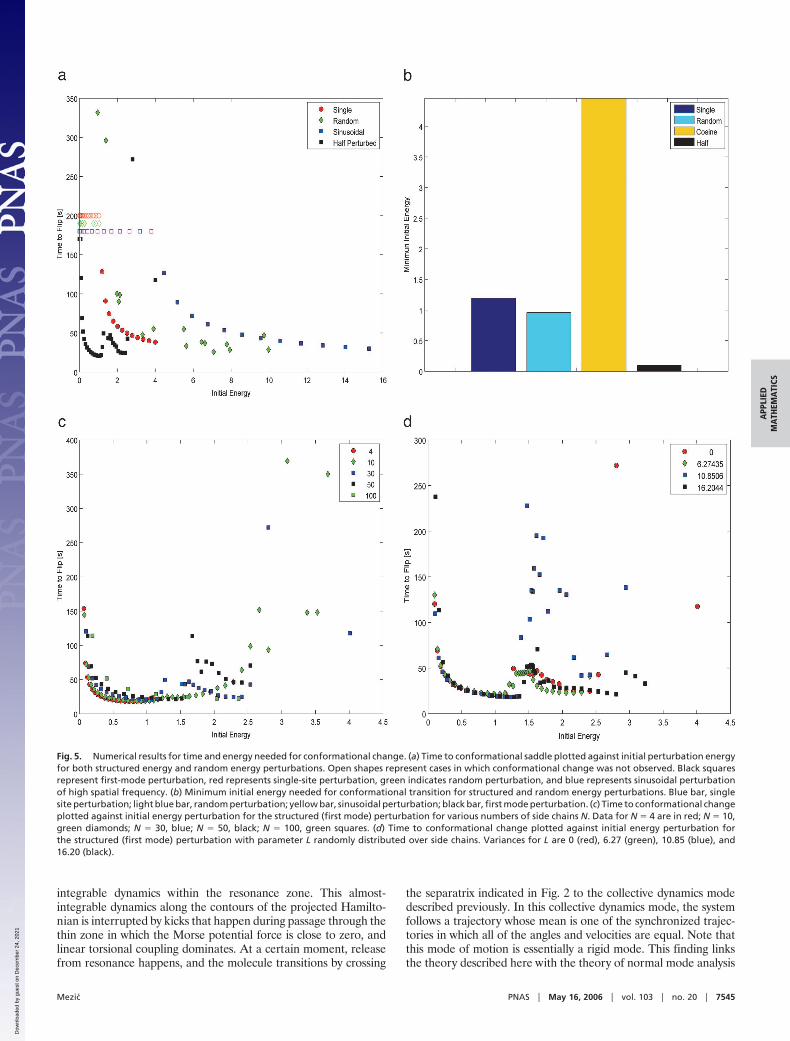
Fig. 5. Numerical results for time and energy needed for conformational change. (a) Time to conformational saddle plotted against initial perturbation energyfor both structured energy and random energy perturbations. Open shapes represent cases in which conformational change was not observed. Black squaresrepresent first-mode perturbation, red represents single-site perturbation, green indicates random perturbation, and blue represents sinusoidal perturbationof high spatial frequency. (b) Minimum initial energy needed for conformational transition for structured and random energy perturbations. Blue bar, singlesite perturbation; light blue bar, random perturbation; yellow bar, sinusoidal perturbation; black bar, first mode perturbation. (c) Time to conformational changeplotted against initial energy perturbation for the structured (first mode) perturbation for various numbers of side chains N. Data for N � 4 are in red; N � 10,green diamonds; N � 30, blue; N � 50, black; N � 100, green squares. (d) Time to conformational change plotted against initial energy perturbation forthe structured (first mode) perturbation with parameter L randomly distributed over side chains. Variances for L are 0 (red), 6.27 (green), 10.85 (blue), and16.20 (black).

Mezic PNAS � May 16, 2006 � vol. 103 � no. 20 � 7545

APP

LIED

MA

THEM

ATI

CS

Dow

nloa

ded

by g

uest

on

Dec

embe

r 24

, 202

1

(NMA; or elastic network models) (4–7) in the sense of theobservation of Delarue and Sanejouand (4) that ‘‘biologicallyrelevant large amplitude motions are essentially rigid body motionsof such domains.’’ The added ingredients introduced here are thenecessity of repulsive–attractive interactions for the transformationof the localized initial disturbances to collective modes and thenecessity of pathways in the phase space that correspond tocollective modes of NMA and connect the conformation zones.These collective modes serve as ‘‘conformational superhighways’’of molecular dynamics.

The last phase in the process of transition is that of the moleculegetting entrained in the resonance zone, around the other exactconformed state. We could say that the whole transition process isin fact ‘‘resonance-enabled.’’

Remarkably, the synchronization described here occurs becauseof a resonance phenomenon in a conservative, locally coupledsystem and does not depend on the dissipativity of the dynamics(18) or global coupling in conservative systems (19). In interestingstudies of Morita and Kaneko (20, 21) of relaxation processes inboth globally and locally coupled conservative systems, collectivebehavior (in the sense of energy accumulation in a particular mode)was observed, leading to large departures from equilibrium beforethe final relaxation process. The phenomena that we describe herealso exhibit collective motion before relaxation. The class of Ham-iltonians that exhibits the particular relaxation process describedhere is different, however, with the requirement of strong localinteractions and weaker global interactions leading to the specificphenomenon that we describe.

Quantitative Analysis of the ModelWe performed a suite of numerical simulations to better under-stand properties of the conformational transition described in theprevious section. In Fig. 5, we show results of an investigation intothe amount of initial energy necessary for conformational changeand its dependence on the structure of the perturbations and thenumber of side chains involved in motion. Note that the energy levelof the saddle located at � � � in the case of 30 side chains is 0.0214.In Fig. 5a we plot time to reach that saddle vs. initial perturbationenergy, which indicates the amount of time it takes to transitionbetween the two conformational equilibria. All of the data areobtained with N � 30 side chains. Four different initial configu-rations are considered. In all of them, initial velocity of all sidechains is zero. Open shapes indicate cases in which transition wasnot achieved. Black squares are data for initial perturbation forwhich half of the side chains are displaced from the equilibrium onthe repulsive side of the potential, and half are in equilibriumposition, corresponding roughly to the first mode of oscillation ofthe linear part of the system. Among all of the nonuniformperturbations studied here, this initial perturbation requires theleast initial energy to perform conformational transition. Thisenergy is an order of magnitude smaller than that of a randomperturbation, the data for which are in green diamonds on the sameplot. This feature is easily seen from Fig. 5b where minimum initialenergy levels for various perturbations are shown. The black barcorresponds to the first-mode perturbation, the light blue to ran-dom energy perturbation. It is interesting to note that even dis-placing a single side chain with all of the others in equilibrium (thedata for which are given in red circles in Fig. 5a and the dynamicsof which was shown in Fig. 3) does better, at the same initial energy,than the random perturbation in terms of how much time it takesto reach the saddle point. The initial energy necessary to induceconformational transition with a single side chain perturbed isshown as a dark blue bar in Fig. 5b and is close to that required bya random perturbation. It is also interesting that structured per-turbations that do not correspond to low oscillation modes of thelinear part of the system do not do very well in terms of minimuminitial energy for conformational flip: the data for time-to-saddle vs.initial energy for a sinusoidal perturbation of the shortest spatial

wavelength around the left conformed state are shown in Fig. 5a inblue squares, and its minimum initial energy is shown as a yellowbar in Fig. 5b. These results are quite robust over a range of N: inFig. 5c we show time-to-saddle vs. initial energy for N � 4, 10, 30,50, and 100 for the first-mode initial condition described above, andwe see that the behavior is qualitatively very similar.

The observed conformational behavior is quite robust to changesin parameter L. We varied individual values Li, i � 1, . . . , N, for N �30 of L for side chains to obtain time-to-saddle vs. initial energydata shown in Fig. 5d for variance in L being 0 (red circles), 6.27(green diamonds), 10.85 (blue squares), and 16.20 (black squares).It is seen that the observed times-to-saddle begin deviating only atthe large variance or �16 where the standard deviation is 40% ofthe mean value of L � 10.

The results described in this section show both that structuredperturbations are better at inducing conformational dynamics in thepresent model than random perturbations are and that such aconclusion holds robustly for a range of side-chain numbers N anddistributions of parameter values Li, i � 1, . . . , N.

GeneralizationThere are three elements of this conformational transition picturethat we consider universal. (i) The first is the existence of exactconformed states in the phase space and relatively stable zones ofintegrable motion around them, that we call conformational sacks.These sacks are governed by effects of attractive�repulsive molec-ular forces and can be detected by using dynamical systems tech-

Fig. 6. Schematic representation of conformational dynamics in phasespace. Areas I and II are conformational sacks. The transition pathway be-tween them is determined by the elastic normal modes of the molecule. Exitsand entrances into conformational sacks are controlled by the resonancedynamics. The transition is initiated by an external, local perturbation at a hotbutton site on the molecule.

7546 � www.pnas.org�cgi�doi�10.1073�pnas.0509028103 Mezic

Dow

nloa

ded

by g

uest

on

Dec

embe

r 24

, 202

1

niques such as the methods for detection of almost-invariant sets(10, 12). (ii) Next is the existence of rapid collective motionsbetween conformational sacks provided by the elastic normalmodes of the molecule. Because these types of motion are preferredby the molecule, the volume of the phase space explored by abiomolecule is minute compared with the total available volume,thus showing that the assumption of equal phase–space probabil-ities that is at the heart of Levinthal argument (2) is not correct. (iii)Targeted localized perturbations can bring about conformationaltransition, by pushing the two adjacent side chains or sets of sidechains into the repulsive domain of their interaction, thus supplyingpotential energy that ultimately gets converted, through the processdescribed above, to kinetic energy of collective-mode-mediatedtransition. This result leads to the conclusion that biological mac-romolecules have ‘‘hot buttons,’’ sites that, when acted on in theright way, lead to global conformational change by means of themechanism of resonance, that involves transition across separatingmanifolds in phase space. This finding is closely related andprovides a mathematical description of the phenomenon of ‘‘pro-tein quakes’’ described by Ansari et al. (8). The schematic of theoverall process is shown in Fig. 6.

There is a large set of N degree-of-freedom Hamiltonians thatare currently used in studies of protein dynamics that satisfy therequirements for the conformational transition that we have de-scribed here. Specifically, these Hamiltonians are of the followingform:

H�q, p� � N�q, p� � L�q, p�,

where p, q are the generalized momentum vector p � (p1, . . . , pN)and generalized position vector q � (q1, . . . , qN). The term N is thenonlinear term coming from nonlocal van der Waals interactionswhereas L(q, p) is the bonded interaction term that contains linearand Fourier terms (see, e.g., ref. 22). In addition to the modelpresented above, we have studied a variety of models of this formthat exhibit similar phenomena to the one presented here. Forexample, a linear model with local harmonic interaction andnonlocal Lennard–Jones interaction that has many conformedequilibria but exhibits transition between an equilibrium in whichthe distances between all of the side chains are the same and large(denatured) to the equilibrium in which all of the distances are thesame and small (conformed). The reason for this transition is theexistence of a normal mode in L that supports it in the waydescribed above. This type of system can serve as a rudimentarymodel of an �-helix secondary structure (22), and its detailed studywill be presented elsewhere.

It is interesting to note that the possibility of using the mechanismof resonance for achieving large changes in dynamical systems usingsmall perturbations has been discussed (23), and it was argued thatexistence of internal resonances of the type described above is a

necessary condition for inducing large changes with small pertur-bations. Methods for computing rates of transition across separatri-ces in high-dimensional Hamiltonian systems have been developedrecently (13) and could be used to further elucidate the motionacross separating manifolds.

ConclusionWe argue here that there are specific structural features of biolog-ical macromolecules that lead to their ability to quickly switchbetween different conformations. The picture that arises is that ofa structure with a reduced number of degrees of freedom, withviable conformations being only those that are accessible throughfast collective motions of the molecule. These fast collective mo-tions are enabled by the local structure, which favors certain modesof motion. The dynamical systems mechanism that allows forefficient use of such motions is that of resonance. The conforma-tions are decided by long-range effects of attractive and repulsiveforces. The switch between two different conformations can beinduced by local perturbations at a specific site in the molecule.Another intriguing related fact is that the dynamics of the moleculeis not chaotic (ergodic) but in fact is piecewise integrable (integrablewithin the resonance zone and with integrable average outside of it;chaotic in the transition). In the case when certain modes ofoscillation are overdamped, it is only the underdamped modes thatcan provide the conformational transition mechanism presentedhere.

Biological macromolecules are oscillator networks with a largenumber of degrees of freedom. They are designed to have func-tionality that is robust to a wide variety of perturbations but also toeasily transform between different configurations when necessary.The essential structural features that allow for this capability arestrong local interconnections (neighbor to neighbor) and globalinterconnections that are weak compared with the local ones,except in the special ‘‘resonance zones.’’ Note that the systemdescribed here acts as a ‘‘switch’’: if we denote the left equilibriumpoint by L and the right equilibrium point by R, the fast transitionbetween the state LLL . . . LLL and RRR . . . RRR is achieved withthe energy input much smaller than expended by moving everysingle L to R individually, thus offering a new advantage formolecular computation (24). The main dynamical feature is thatstrong local interconnections provide fast pathways between zonesin the phase space in which long-range forces dominate. Thus, wecontend that we can learn a lot about designing robust flexiblenetworks by studying design of biological macromolecules.

I thank Bryan Eisenhower for providing some of the numerical simu-lations and Andrzej Banaszuk, Jerry Marsden, and Philip de Toit foruseful comments. This work was supported in part by grants from theDefense Advanced Research Projects Agency and the Air Force Officeof Scientific Research.

1. Komatsuzaki, T. & Berry, R. S. (2002) J. Phys. Chem. A 106, 10945–10950.2. Levinthal, C. (1969) in Mossbauer Spectroscopy in Biological Systems: Proceed-

ings of a Meeting Held at Allerton House, Monticello, Illinois, eds. Debrunner, P.,Tsibris, J. & Munck, E. (Univ. of Illinois Press, Urbana–Champaign), pp. 22–24.

3. Mayor, U., Guydosh, N. R., Johnson, C. M., Grossmann, J. G., Sato, S., Jas,G. S., Freund, S. M. V., Alonso, D. O. V., Daggett, V. & Fersht, A. R. (2003)Nature 421, 863–867.

4. Delarue, M. & Sanejouand, Y.-H. (2002) J. Mol. Biol. 320, 1011–1024.5. Go, O., Noguti, T. & Nishikawa, T. (1983) Proc. Natl. Acad. Sci. USA 80,

3696–3700.6. Bahar, I., Atligan, A. R. & Erman, B.-B. (1997) Folding Des. 2, 13034–13039.7. Hinsen, K. (1998) Proteins Struct. Funct. Genet. 33, 417–429.8. Ansari, A., Berendzen, J., Bowne, S. F., Frauenfelder, H., Iben, I. E. T., Sauke,

T. B., Shyamsunder, E. & Young, R. D. (1985) Proc. Natl. Acad. Sci. USA 82,5000–5004.

9. Peyrard, M. & Bishop, A. R. (1989) Phys. Rev. Lett. 62, 2755–2758.10. Dellnitz, M. & Junge, O. (2002) in Handbook of Dynamical Systems II: Towards

Applications, eds. Fiedler, B., Iooss, G. & Kopell, N. (World Scientific, NewYork), pp. 221–264.

11. Peyrard, M. (2004) Nonlinearity 17, R1–R40.12. Deuflhard, P. & Schutte, C. (2004) in Applied Mathematics: Entering the 21st

Century, Proceedings in Applied Mathematics, eds. Hill, J. M. & Moore, R.(Soc. for Industrial and Appl. Math., Philadelphia), Vol. 116, pp. 91–119.

13. Gabern, F., Koon, W. S. & Marsden, J. E. (2005) Physica D 212, 271–304.14. Englander, S., Kallenbach, N., Heeger, A. J., Krumshansl, J. & Litwin S. (1980)

Proc. Natl. Acad. Sci. USA 77, 7222–7226.15. Honeycutt, J. D. & Thirumalai, D. (1992) Biopolymers 32, 659–709.16. Brown, S., Fawzi, N. J. & Head-Gordon, T. (2003) Proc. Natl. Acad. Sci. USA

100, 10712–10717.17. Neishtadt, A. (1997) Celestial Mech. Dyn. Astron. 111, 1–20.18. Mirollo, R. E. & Strogatz, S. H. (1990) SIAM J. Appl. Math. 50, 1645–1662.19. Smereka, P. (1998) Physica D 124, 104–125.20. Morita, H. & Kaneko, K. (2004) Europhys. Lett. 66, 198–204.21. Morita, H. & Kaneko, K. (2005) Phys. Rev. Lett. 94, 087203-1–087203-4.22. Schlick, T. (2002) Molecular Modelling and Simulation, Interdisciplinary Ap-

plied Mathematics (Springer, Heidelberg, Germany), Vol. 21.23. Vainchtein, D. & Mezic, I. (2004) Phys. Rev. Lett. 93, 084301-1–084301-4.24. Adleman, L. M. (1994) Science 266, 1021–1024.

Mezic PNAS � May 16, 2006 � vol. 103 � no. 20 � 7547

APP

LIED

MA

THEM

ATI

CS

Dow

nloa

ded

by g

uest

on

Dec

embe

r 24

, 202

1