On the Distributions of Infinite Server Queues withBatch Arrivals

Andrew DawSchool of Operations Research and Information Engineering

Cornell University257 Rhodes Hall, Ithaca, NY 14853

amd399@cornell.edu

Jamol PenderSchool of Operations Research and Information Engineering

Cornell University228 Rhodes Hall, Ithaca, NY 14853

jjp274@cornell.edu

February 5, 2019

Abstract

Queues that feature multiple entities arriving simultaneously are among the oldestmodels in queueing theory, and are often referred to as “batch” (or, in some cases,“bulk”) arrival queueing systems. In this work we study the affect of batch arrivalson infinite server queues. We assume that the arrival epochs occur according to aPoisson process, with treatment of both stationary and non-stationary arrival rates.We consider both exponentially and generally distributed service durations and weanalyze both fixed and random arrival batch sizes. In addition to deriving the transientmean, variance, and moment generating function for time-varying arrival rates, wealso find that the steady-state distribution of the queue is equivalent to the sum ofscaled Poisson random variables with rates proportional to the order statistics of itsservice distribution. We do so through viewing the batch arrival system as a collectionof correlated sub-queues. Furthermore, we investigate the limiting behavior of theprocess through a batch scaling of the queue and through fluid and diffusion limits ofthe arrival rate. In the course of our analysis, we make important connections betweenour model and the harmonic numbers, generalized Hermite distributions, and truncatedpolylogarithms.

1 Introduction

Queueing systems with batch arrivals have enjoyed a long and rich history of study,at least on the time scale of queueing theory. Researchers have been exploring models

1

arX

iv:1

805.

0211

7v3

[m

ath.

PR]

2 F

eb 2

019

of this sort for no less than six decades, based on the April 1958 submission date ofMiller Jr [26]. Given this stretch of time, a wide variety of systems and settings havebeen considered under the banner of batch arrivals. Much of the earliest work focuseson single server models, including Miller Jr [26], Lucantoni [22], Masuyama and Takine[25], Liu and Templeton [20] and Foster [12], although infinite server models followedsoon after, such as work by Shanbhag [36] and Brown and Ross [2]. Later work hasexpanded the concept into a variety of related models, such as for priority queues [37]and for handling server vacations [19]. Additionally, there is some work that provesheavy traffic limit theorems for queues with batch arrivals. Examples of this includeChiamsiri and Leonard [3], Pang and Whitt [28], Pender [29]. These papers show thatone can approximate the queue length process with Brownian motion and Ornstein-Uhlenbeck processes and also show that one can exploit the approximations even inmulti-server and non-Markovian settings.

In this paper we consider queues with arrivals occurring at times following a Poissonprocess, with consideration given to both non-stationary and stationary rates. Weanalyze both both general and exponential service as conducted by infinitely manyservers. Additionally, this work addresses both fixed and random batch sizes. Ouranalysis starts with the fixed batch size case. We begin by analyzing the transientbehavior of the queue with Markovian service and time-varying arrival rates, providingexplicit forms for the moment generating function, mean, and variance. Then, weshow that if the arrival rate is stationary the resulting steady-state distribution canbe written as a sum of independent, non-identical, scaled Poisson random variables.This leads us to uncover connections to the harmonic numbers and generalizations ofthe Hermite distribution. By viewing the batch arrival queue as a collection of infiniteserver sub-queues that receive solitary arrivals simultaneously, we are able to extendthis Poisson sum construction to general service distributions. This perspective alsoprovides an avenue for us to extend to random batch sizes. We also give fluid anddiffusion scalings of the queue in the case of random batch sizes, as well as extendingmany of the results we found for fixed batch sizes.

One can note that the batch arrival queue may not always be given the name“batch,” as many authors choose to use the term “bulk” instead. Predominantly, thisreflects two leading strands of applications, where “bulk” often gives a connotation oftransportation settings whereas “batch” frequently implies applications in communica-tions. Just as practical by any other name, this family of models has also been studiedin a wide variety of applications beyond these two. Perhaps one most distinct fromother types of queueing models is particle splitting in DNA caused by radiation, asdiscussed in Sachs et al. [35]. In this application, primary particles arrive at a cell nu-cleus and cause DNA double-strand breaks. These double-strand breaks occur in nearsimultaneity and are thus modeled as arriving in batches of random size, as it is possi-ble that any number double-strand breaks will be induced. After they are induced, thedouble-strand breaks are then processed by cellular enzymes, corresponding to servicein the queueing model. Another interesting and modern application of these modelsis in cloud-based data processing. In this case, the batches arriving to the system arecollections of jobs submitted simultaneously. These jobs are then served by each beingprocessed individually and returned. For more discussion, detailed models, and spe-cific analysis for this setting, see works such as Lu et al. [21], Pender and Phung-Duc[31], Xie et al. [38], Yekkehkhany et al. [39] and references therein.

2

1.1 Main Contributions of Paper

Our contributions in this work can be summarized as follows:

i) We show that an infinite server queue with batch arrivals at Poisson processepochs is equivalent in steady state distribution to a sum of scaled independentPoisson random variables, including for generally distributed service and ran-domly distributed batch sizes. For exponential service, this reveals a connectionto the harmonic numbers and generalized Hermite distributions.

ii) We derive a limit of the process in which the batch size grows infinitely large andthe number of entities in the system is scaled inverse proportionally, yielding anovel distribution characterized by the exponential integral functions. For distri-butions that meet a divisibility condition, we find that this also holds for randombatch sizes.

iii) In the case of time-varying arrival rates we give a transient moment generatingfunction for fixed batch sizes as well as means and variance for both fixed andrandomly sized batches.

iv) We give fluid and diffusion limits of the queue for stationary arrival rates forbatches of random size.

1.2 Organization of Paper

The body of the remainder of this paper is organized in two main sections: Sections 2and 3. In Section 2 we consider systems in which the size of the batches is fixed.Similarly, we devote Section 3 to the case of randomly distributed batch sizes. Atthe beginning of each section we give a detailed overview of the contents within andprovide context for the analysis in term of this project’s scope. After these sections weconclude in Section 4.

2 Batches of Deterministic Size

In this section we will consider infinite server queues with arrivals occurring in batchesof a fixed size. We will assume that the arrival epochs occur according to a Poissonprocess, including both stationary and non-stationary models. We also will investigateboth exponentially and generally distributed service.

This section starts with studying the case of Markovian arrivals and service intransient state in Subsection 2.1. For a time-varying arrival rate, we give the mean,variance, and moment generating function. We then use this in Subsection 2.2 to findthe steady-state distribution of the queue. Upon observing that this can be representedas a sum of scaled Poisson random variables, we establish connections to generalizedHermite distributions and to the harmonic numbers. Taking motivation from this, wederive the distribution of the limit of the scaled system as the batch size grows infinitelylarge. Finally, in Subsection 2.3, we examine the batch queue as a collection of infiniteserver sub-queues that simultaneously receive solitary arrivals. In doing so we extendour understanding of the steady-state distribution to the case of general service.

3

2.1 Transient Analysis of the Markovian Setting

We begin our analysis with the case of non-stationary Poisson arrival epochs andMarkovian service. In Kendall notation, this is the Mn

t /M/∞ queue. We let Qtrepresent the number of entities present in the queueing system at time t ≥ 0, whichwe often refer to as the “number in system.” We will use this notation throughoutthe remainder of this work, where the precise setting of the queue will be implied bycontext. In this fully Markovian setting, we can use Dynkin’s infinitesimal generatortheorem to support our analysis. Specifically, we can note that for a sufficiently regularfunction f : N→ R, we have

d

dtE [f(Qt)] = E [λ(t) (f(Qt + n)− f(Qt)) + µQt (f(Qt − 1)− f(Qt))], (2.1)

for a batch arrival queue with arrival intensity λ(t) > 0. We will see in this subsectionthat this infinitesimal generator approach gives us a potent toolkit for exploring thismodel. Moreover, the insights we find in Markovian settings now and in Subsection 2.2will provide intuition that will guide our investigation of this system when the Markovproperty does not hold. To begin, we now derive the moment generating function ofthe number in system. We do so for a system with a non-stationary arrival rate givenby a Fourier series, allowing these results to hold for all periodic arrival patterns.

Proposition 2.1. For θ ∈ R, letM(θ, t) = E[eθQt

]be the moment generating function

of the number in system of an infinite server queue with periodic arrival rate λ +∑∞k=1 ak cos(kt) + bk sin(kt) > 0, arrival batch size n ∈ Z+, and exponential service

rate µ > 0. Then, M(θ, t) is given by

M(θ, t) =(e−µt(eθ − 1) + 1

)Q0

e∑nj=1 (nj)(eθ−1)j

(λjµ(1−e−jµt)+

∑∞k=1

(akjµ−bkk)k2+j2µ2

(cos(kt)−e−jµt))

· e∑nj=1 (nj)(eθ−1)j

∑∞k=1

(akk+bkjµ) sin(kt)

k2+j2µ2 (2.2)

for all time t ≥ 0, where Q0 is the initial number in system.

Proof. From Equation 2.1, the MGF is given by the solution to the partial differentialequation

∂

∂tM(θ, t) =

(λ+

∞∑k=1

ak cos(kt) + bk sin(kt)

)(enθ − 1

)M(θ, t) + µ

(e−θ − 1

) ∂

∂θM(θ, t)

with initial solution M(θ, 0) = eθQ0 . Because d log(f(x))dx = 1

f(x)df(x)

dx , we can observe

that the partial differential equation for the cumulant generating function G(θ, t) =log(E[eθQt

])is

µ(1− e−θ)∂G(θ, t)

∂θ+∂G(θ, t)

∂t=

(λ+

∞∑k=1

ak cos(kt) + bk sin(kt)

)(enθ − 1),

with the initial condition G(θ, 0) = log(E[eθQ0

])= θQ0. We will now solve this PDE

by the method of characteristics. We begin by establishing the characteristic ODE’s

4

and corresponding initial solutions as follows:

dθ

ds(r, s) = µ(1− e−θ), θ(r, 0) = r,

dt

ds(r, s) = 1, t(r, 0) = 0,

dg

ds(r, s) =

(λ+

∞∑k=1

ak cos(kt) + bk sin(kt)

)(enθ − 1), g(r, 0) = rQ0.

The first two of these initial value problems yield the following solutions.

θ(r, s) = log(ec1(r)+µs + 1) → θ(r, s) = log ((er − 1)eµs + 1)

t(r, s) = s+ c2(r) → t(r, s) = s

Therefore we can simplify the remaining characteristic ODE to

dg

ds(r, s) =

(λ+

∞∑k=1

ak cos(ks) + bk sin(ks)

)(((er − 1)eµs + 1)n − 1)

=

(λ+

∞∑k=1

ak cos(ks) + bk sin(ks)

)n∑j=1

(n

j

)(er − 1)jejµs,

and this produces the general solution of

g(r, s) = c3(r) +

n∑j=1

(n

j

)(er − 1)j

(λ

jµ+

∞∑k=1

(akjµ− bkk) cos(ks)

k2 + j2µ2+

(akk + bkjµ) sin(ks)

k2 + j2µ2

)ejµs.

This now equates to

g(r, s) = rQ0 +n∑j=1

(n

j

)(er − 1)j

(λ

jµ

(ejµs − 1

)+∞∑k=1

(akjµ− bkk)

k2 + j2µ2

(cos(ks)ejµs − 1

)+∞∑k=1

(akk + bkjµ) sin(ks)

k2 + j2µ2ejµs

)

as the solution to the initial value problem. We now find the solution to the originalPDE by solving for each characteristic variable in terms of t and θ and then substitutingthese expression into g(r, s). That is, for s = t and r = log

(e−µt(eθ − 1) + 1

), we have

that

G(θ, t) = g(

log(e−µt(eθ − 1) + 1

), t)

= log(e−µt(eθ − 1) + 1

)Q0 +

n∑j=1

(n

j

)(eθ − 1)j

(λ

jµ

(1− e−jµt

)+

∞∑k=1

(akjµ− bkk)

k2 + j2µ2

·(cos(kt)− e−jµt

)+

∞∑k=1

(akk + bkjµ)

k2 + j2µ2sin(kt)

).

To conclude the proof, we note that M(θ, t) = eG(θ,t).

5

We now extend this analysis through two following corollaries. First, for systemswith a stationary arrival rate, say λ > 0, we can further specify the moment generatingfunction explicitly in Corollary 2.2. This will be of use when we explore the distributionof the queue in steady-state, which we begin in Subsection 2.2. As with Proposition 2.1,the uniqueness of moment generating functions will aid us in later exploration of thedistributions within this model and within generalizations of it.

Corollary 2.2. For θ ∈ R, let M(θ, t) = E[eθQt

]be the moment generating function

of the number in system of an infinite server queue with stationary arrival rate λ > 0,arrival batch size n ∈ Z+, and exponential service rate µ > 0. Then, M(θ, t) is givenby

M(θ, t) =(e−µt(eθ − 1) + 1

)Q0

eλ∑nj=1 (nj)

(eθ−1)j

jµ (1−e−jµt) (2.3)

for all time t ≥ 0, where Q0 is the initial number in system.

For the second direct result of Proposition 2.1, we can also give explicit expres-sions for the transient mean and variance of the queue. We derive these equationsfrom the first and second derivatives, respectively, of the cumulant generating functionlog(E

[eQt]).

Corollary 2.3. Let Qt be an infinite server queue with periodic arrival rate λ +∑∞k=1 ak cos(kt) + bk sin(kt) > 0, arrival batch size n ∈ Z+, and exponential service

rate µ > 0. Then, the mean and variance of the queue are given by

E [Qt] = Q0e−µt +

nλ

µ

(1− e−µt

)+

∞∑k=1

n(akµ− bkk)

k2 + µ2

(cos(kt)− e−µt

)+

∞∑k=1

n(akk + bkµ)

k2 + µ2sin(kt) (2.4)

Var (Qt) = Q0

(e−µt − e−2µt

)+nλ

µ

(1− e−µt

)+

∞∑k=1

n(akµ− bkk)

k2 + µ2

(cos(kt)− e−µt

)+∞∑k=1

n(akk + bkµ)

k2 + µ2sin(kt) +

n(n− 1)λ

2µ

(1− e−2µt

)+∞∑k=1

n(n− 1)(2akµ− bkk)

k2 + 4µ2

·(cos(kt)− e−2µt

)+∞∑k=1

n(n− 1)(akk + 2bkµ)

k2 + 4µ2sin(kt) (2.5)

for all time t ≥ 0, where Q0 is the initial number in system.

In the remainder of this work we will explore various modifications of this model,including general service and randomized batch sizes. The results of this subsectionwill serve as cornerstone throughout much of this upcoming analysis, both supportingthe underlying derivation techniques and providing the intuition for new perspectives.

2.2 The Markovian System with Stationary Arrival Rates

Our first departure from our initial model will be modest: instead of studying the fullyMarkovian, non-stationary, fixed batch size system in transient time we will now move

6

to addressing the stationary case, with much of our analysis focused on the system insteady-state. This simplified setting will allow us to extract greater intuition from ourprior findings, which in turn will support generalization of the service distribution andrandomization of the batch sizes. To begin, we find a representation of the steady-state distribution of the queue length in terms of a sum of independent, scaled Poissonrandom variables.

Proposition 2.4. In steady-state the distribution of the number in system of an in-finite server queue with stationary arrival rate λ > 0, arrival batch size n ∈ Z+, andexponential service rate µ > 0 is

Q∞(n)D=

n∑j=1

jYj (2.6)

where Yj ∼ Pois(λjµ

)are independent.

Proof. From Proposition 2.1, we have that the steady-state moment generating func-tion of the queue is given by

limt→∞M(θ, t) = e

λ∑nk=1 (nk)

(eθ−1)k

kµ .

To satisfy our stated Poisson form, we are now left to show that∑n

k=1

(nk

) (eθ−1)k

k =∑nk=1

ekθ−1k for all n ∈ Z+. We proceed by induction. In the base case of n = 1

we have eθ − 1 = eθ − 1 and so we are left to show the inductive step. We now

assume∑n

k=1

(nk

) (eθ−1)k

k =∑n

k=1ekθ−1k holds at n. Then, by the Pascal triangle identity(

nk

)=(n+1k

)−(nk−1

)and our inductive hypothesis we can observe

n∑k=1

ekθ − 1

k=

n∑k=1

(n

k

)(eθ − 1)k

k=

n∑k=1

((n+ 1

k

)−(

n

k − 1

))(eθ − 1)k

k.

Now, by applying the identity(nk−1

)= k

n+1

(n+1k

)and distributing the summation we

can further note thatn∑k=1

((n+ 1

k

)−(

n

k − 1

))(eθ − 1)k

k=

n∑k=1

((n+ 1

k

)− k

n+ 1

(n+ 1

k

))(eθ − 1)k

k

=n∑k=1

(n+ 1

k

)(eθ − 1)k

k−∑n

k=1

(n+1k

)(eθ − 1)k

n+ 1.

Now, we can use the binomial theorem to see that

n∑k=1

(n+ 1

k

)(eθ − 1)k = (eθ − 1 + 1)n+1 − 1− (eθ − 1)n+1 = e(n+1)θ − 1− (eθ − 1)n+1,

and so we can now simplify and find

n∑k=1

(n+ 1

k

)(eθ − 1)k

k−∑n

k=1

(n+1k

)(eθ − 1)k

n+ 1=

n∑k=1

(n+ 1

k

)(eθ − 1)k

k+

(eθ − 1)n+1

n+ 1

− e(n+1)θ − 1

n+ 1.

7

Hence, in conjunction with our initial equation, we have that

n∑k=1

ekθ − 1

k=

n∑k=1

(n+ 1

k

)(eθ − 1)k

k+

(eθ − 1)n+1

n+ 1− e(n+1)θ − 1

n+ 1,

and by rearranging terms we now complete the inductive approach:

n+1∑k=1

ekθ − 1

k=

n+1∑k=1

(n+ 1

k

)(eθ − 1)k

k.

We can now observe that we have a moment generating function that is a productof moment generating functions of scaled Poisson random variables, which yields thestated result.

While we will continue to explore the stationary arrival rate setting throughout thissubsection, we note that this Poisson sum representation will be a leading inspirationin the sequel. Specifically, in Subsection 2.3 we will find intuition for this result byviewing the batch arrival queue as a collection of sub-systems.

Remark. In addition to this Poisson sum representation, we can also express the steady-state MGF in terms of the truncated polylogarithm function and harmonic numbers.From the MGF of the queue length in steady state for θ < 0, we can observe that

limt→∞M(θ, t) = e

λµ

∑nk=1

ekθ−1k = e

λµ

(Li(eθ,n,1)−Hn)

where we have Hn as the nth harmonic number, given by∑n

k=11k , and where the

truncated polylogarithm function Li(z, n, s) is defined as

Li(z, n, s) =n∑k=1

zk

ks.

This decomposition into Poisson random variables can be quite useful from a com-putational standpoint. It allows us to simulate the steady state quite easily since weonly need to simulate n Poisson random variables instead of simulating an actual queue,which could be quite expensive. We can now observe that this construction also yieldsan interesting connection to both the harmonic number and Hermite distributions, assuggested in the remark above. To motivate our following analysis, suppose that n = 2.Then, steady-state queue length has steady-state moment generating function given by

Mn(θ,∞) = eλµ(eθ−1)+ λ

2µ(e2θ−1).

We can now observe that this MGF corresponds to a Hermite distribution with pa-rameters λ

µ and λ2µ . This implies that the steady-state CDF of the queue at n = 2

is

P (Q∞(2) ≤ k) = e− 3λ

2µ

bkc∑i=0

bi/2c∑j=0

(λµ

)i−2j (λ2µ

)j(i− 2j)!j!

= e− 3λ

2µ

bkc∑i=0

bi/2c∑j=0

(λµ

)i−j2−j

(i− 2j)!j!.

8

Furthermore, the steady-state PMF of the queue length is given by

P (Q∞(2) = i) = e− 3λ

2µ

bi/2c∑j=0

(λµ

)i−j2−j

(i− 2j)!j!.

This observation prompts us to ponder generalizations for n ≥ 3. The term “generalizedHermite distribution” has taken on slightly varying (yet always interesting) definitionsfor different authors. For readers interested in the Hermite distribution and populargeneralizations of it, we suggest Kemp and Kemp [16], Gupta and Jain [14], and Milneand Westcott [27]. In our setting we note that the coefficients of λµ in the MGF for batch

size n will be 1, 12 , 1

3 , . . . , 1n . For this reason, we think of this particular generalization of

Hermite distributions to be the harmonic Hermite distribution. We can now note thatbecause of this harmonic structure we can instead fully characterize the distributionsimply by n and λ

µ . In the following proposition we find a useful recursion for the

probability mass function of this distribution at all n ∈ Z+.

Proposition 2.5. Let Qt(n) be an infinite server batch arrivals queue with arrival rateλ > 0, batch size n ∈ Z+, and service rate µ > 0. Then, the steady-state distributionof the queue is given by the recursion

P(Q∞(n) = j) = pj =n∑i=1

ipj−iλ

ijµ=

n∑i=1

pj−iλ

jµ, (2.7)

where p0 = e−λµHn for Hn as the nth harmonic number and pk = 0 for all k < 0. Thus,

we say that Q∞(n) follows the “harmonic Hermite distribution” with parameter n.

Proof. We know from our Poisson representation of the steady state queue length thatthe steady-state moment generating function is

M(θ) =∞∑j=0

P(Q∞(n) = j)θj =∞∑j=0

pjθj = exp

(n∑i=1

λ

iµ

(θi − 1

)).

If we take the logarithm of both sides we see that we have

log

∞∑j=0

pjθj

=n∑i=1

λ

iµ

(θi − 1

).

Now we take the derivative of both sides with respect to the parameter θ and thisyields the following expression∑∞

j=1 jpjθj−1∑∞

j=0 pjθj

=

n∑i=1

λ

µθi−1.

By moving the denominator to the righthand side, we have that

∞∑j=1

jpjθj−1 =

∞∑j=0

pjθj

( n∑i=1

λ

µθi−1

).

Finally, by matching similar powers of θ on the left and right sides, we complete theproof.

9

From the above result, we see that for the steady state queue length Q∞(n) we canderive the specific probabilities,

p0 = e−λµHn ,

p1 =λ

µp0 =

λ

µe−λµHn ,

p2 =λ

2µ(p0 + p1) =

λ

2µe−λµHn +

λ2

2µ2e−λµHn .

We can repeat this process as needed for any desired probability. From Proposition 2.4,we can observe that the mean number in system grows linearly with the batch size,meaning that the mean of the nth harmonic Hermite distribution is

E [Q∞(n)] =n∑j=1

jE [Yj ] =nλ

µ. (2.8)

We can observe further that the second moment and variance are quadratic functionsof n:

E[Q∞(n)2

]= E

n∑j=1

jYj

2 =n(n+ 1)λ

2µ+ n2λ

2

µ2,

Var[Q∞(n)] = E[Q∞(n)2

]− E [Q∞(n)]2 =

n(n+ 1)λ

2µ.

We note that from Proposition 2.4 and the following remark, the moment generatingfunction of this distribution is given by

limt→∞M(θ, t) = e

λµ

∑nk=1

ekθ−1k = e

λµ

(Li(eθ,n,1)−Hn). (2.9)

If one is to consider this system as the batch size grows infinitely large we can see fromEquations 2.8 and 2.9 that the number in system will grow proportionally, tending toinfinity as n does. This leads us to ponder the limiting object of the scaled number insystem Qt(n)

n as the batch size grows.

We begin by using Equation 2.9 with θ replaced by θn to see that the steady-state

moment generating function of this scaled queue length is

limt→∞M(θ, t) = e

λµ

∑nk=1

ekn θ−1k . (2.10)

Furthermore, by replacing θ with θn and Q0(n) with Q0(n)

n in Proposition 2.1, we cannote that the transient moment generating function for this scaled system with constantarrival rate is given by

E[eθ·

Qt(n)n

]≡Mn(θ, t) =

(e−µt(e

θn − 1) + 1

)Q0neλ∑nk=1 (nk)

(eθ/n−1)k

kµ (1−e−kµt).

Additionally, we can also observe that the steady-state distribution of the scaled queuecan also be interpreted as a sum of Poisson random variables through direction ap-plication of Proposition 2.4 or by inspection of Equation 2.10. This representation

10

is

Q∞(n)

n

D=

n∑j=1

j

nYj , (2.11)

where again Yj ∼ Pois(λjµ

).

We now consider the limit as n → ∞, in which we are both sending the size ofbatches of arrivals to infinity while also scaling the size of the queue inversely. We canuse this construction to move beyond just the mean and variance and instead explicitlystate every cumulant of the scaled queue. In Proposition 2.6 we give exact expressionsof all steady-state cumulants of the scaled queue as functions of the Bernoulli numbers.Further, we find a convenient form of every cumulant of the scaled queue as the batchsize grows to infinity.

Proposition 2.6. Let λ > 0 be the arrival rate of batches of size n ∈ Z+ to an infiniteserver queue with exponential service rate µ > 0. Then, the kth steady-state cumulant

of the scaled queue Ck[Q∞(n)n

]is given by

Ck[Q∞(n)

n

]=

nk

k + 12n

k−1 +∑k−1

j=2Bjj! (k − 1)j−1n

k−j

nk. (2.12)

where (n)i = n!(n−i)! is the ith falling factorial of n and Bi is the ith Bernoulli number,

which is defined as

Bi =i∑

k=0

k∑j=0

(−1)j(k

j

)(j + 1)i

k + 1.

Moreover, we have that limn→∞ Ck[Q∞(n)n

]= λ

kµ .

Proof. From our prior observation that Q∞(n)n

D=∑n

j=1jnYj where Yj ∼ Pois

(λjµ

), we

have that

Ck[Q∞(n)

n

]= Ck

n∑j=1

j

nYj

=n∑j=1

Ck[j

nYj

]=

n∑j=1

jk

nkCk [Yj ] =

λ

µnk

n∑j=1

jk−1,

from the independence of these Poisson distributions. Now, by using Faulhaber’s for-mula as given in Knuth [17], we achieve the stated result.

Just as we built from inherited expressions for the mean and variance to specifyevery cumulant in Proposition 2.6, we can also find the limit of the transient-statemoment generating function for the scaled queue given in Equation 2.9.

Proposition 2.7. Let Qt be an infinite server queue with arrival rate λ > 0, arrivalbatch size n ∈ Z+, and exponential service rate µ > 0. For θ ∈ R, let

M∞(θ, t) = limn→∞

E[eθQt(n)n

].

11

Then, M∞(θ, t) is given by

M∞(θ, t) =

eλµ(Ei(θ)−Ei(θe−µt)−µt) if θ > 0,

eλµ(E1(−θe−µt)−E1(−θ)−µt) if θ < 0,

1 if θ = 0,

(2.13)

for all time t ≥ 0, where the exponential integral functions Ei(x) and E1(x) are defined

Ei(x) = −∫ ∞−x

e−s

sds, E1(x) =

∫ ∞x

e−s

sds,

and are real-valued for x > 0.

Proof. While conventions may vary by application area, in this work we use the defi-nition of exponential integral function given by

Ei(x) = −∫ ∞−x

e−s

sds.

By taking the limit of the MGF of the scaled queue, we have that

∂

∂tM∞(θ, t) = λ

(eθ − 1

)M∞(θ, t)− µθ ∂

∂θM∞(θ, t)

with initial solution M∞(θ, 0) = limn→∞ eθQ0n = 1. In the same manner as the proof

of Theorem 2.1, we solve the PDE of the cumulant generating function through use ofthe method of characteristics. We start by establishing the characteristic ODE’s:

dθ

ds(r, s) = µθ, θ(r, 0) = r,

dt

ds(r, s) = 1, t(r, 0) = 0,

dg

ds(r, s) = λ(eθ − 1), g(r, 0) = 0.

We now solve the first two initial value problems and find

θ(r, s) = c1(r)eµs → θ(r, s) = reµs,

t(r, s) = s+ c2(r) → t(r, s) = s.

This allows us to simplify the third characteristic equation to

dg

ds(r, s) = λ(ere

µs − 1).

Because θ = reµs, we can note that r and θ will match in sign: r > 0 if and only ifθ > 0. If θ > 0, the general solution to this ODE is

g(r, s) = c3(r) +λ

µ(Ei(reµs)− µs) ,

whereas if θ < 0, the solution is instead

g(r, s) = c3(r)− λ

µ(E1(−reµs) + µs) .

12

This follows from the fact that for x > 0 the exponential integral functions are suchthat Ei(x) = −E1(−x)− iπ; that is, the real parts of E1(−x) and −Ei(x) are the same.Moreover, for x > 0 one can consider Ei(x) as the real part of −E1(−x). Additionally,E1(x) is real for all x > 0. Hence, we use each definition of the exponential integralfunction when appropriate. As an alternative, we could replace each of these functionswith real(−E1(−x)) to have a single expression for both positive and negative x. Fora collection of facts regarding the exponential integral functions, see Pages 228-237 ofAbramowitz and Stegun [1].

Now, using this we have that the corresponding solutions to the initial value prob-lems will be

g(r, s) =

{λµ (Ei(reµs)− Ei(r)− µs) if r > 0,λµ (E1(−r)− E1(−reµs)− µs) if r < 0.

Hence, for s = t and r = θe−µt, this yields

G(θ, t) = g(θe−µt, t

)=

{λµ

(Ei(θ)− Ei(θe−µt)− µt

)if θ > 0,

λµ

(E1(−θe−µt)− E1(−θ)− µt

)if θ < 0.

By M∞(θ, t) = eG∞(θ,t), we complete the proof.

By consequence, we can also give the moment generating function in steady-state.

Corollary 2.8. The moment generating function of the scaled number in system insteady-state as n→∞ is given by

M∞(θ) =

θ−λµ e

λµ

(Ei(θ)−γ)if θ > 0,

(−θ)−λµ e−λµ

(E1(−θ)+γ)if θ < 0,

1 if θ = 0,

(2.14)

where γ is the Euler-Mascheroni constant.

Proof. From Abramowitz and Stegun [1], for x > 0 we can expand the exponentialintegral functions as

Ei(x) = γ + log(x) +

∞∑k=1

xk

kk!, E1(x) = −γ − log(x)−

∞∑k=1

(−x)k

kk!, (2.15)

where γ is the Euler-Mascheroni constant. By expanding Ei(θe−µt) and E1(−θe−µt)in the respective cases of positive and negative θ and taking the limit as t → ∞, weachieve the stated result.

As a demonstration of the convergence of the steady-state moment generating func-tions of the batch scaled queues to the expression given in Corollary 2.8, we plot thefirst four cases in comparison to the limiting scenario in Figure 2.1.

While it can be argued that even in steady-state the form of this moment generatingfunction is unfamiliar, we can still observe interesting characteristics of it. In particular,for θ < 0 we can uncover a connection back to the harmonic numbers. We now discussthis in the following remark.

13

Figure 2.1: Steady-state MGF of the scaled queue for increasing batch size where λµ

= 1.

Remark. Using Equation 2.15, we can note that for θ < 0 the steady-state momentgenerating function of limit of the scaled queue can be expressed

M(θ) = (−θ)−λµ e−λµ

(E1(−θ)+γ)= e−λµ

(E1(−θ)+γ+log(−θ))= e−λµ

(−∑∞k=1

θk

kk!

).

From Dattoli and Srivastava [4], we have that −ex∑∞

k=1(−x)k

kk! is an exponential gen-erating function for the harmonic numbers. That is,

−ex∞∑k=1

(−x)k

kk!=

∞∑n=1

xn

n!Hn

where Hn is the nth harmonic number. Thus, for θ < 0 the steady-state momentgenerating function of this limiting object can be further simplified to

M(θ) = e−λµ

(−∑∞k=1

θk

kk!

)= e−λµ

∑∞n=1Hne

θ (−θ)nn! = e

−λµ

E[HN ],

where N ∼ Pois(−θ).In addition to this remark’s connection of the moment generating function and the

harmonic numbers, we can also gain insight into this limiting object through MonteCarlo methods. Using Equation 2.11, we have a simple and efficient approximate sim-ulation method for this process through summing scaled Poisson random numbers.Furthermore, this approximation of course becomes increasingly precise as n grows.As an example of this, we give the simulated steady-state densities across differentrelationships of λ and µ in Figures 2.2. In addition to the interesting shapes of thedensities across the different settings, one can see the limiting form of the relationshipsgiven by the recursion in Proposition 2.5 in these plots. We can note that one could also

14

calculate these through a numerical inverse Laplace transform of the steady-state mo-ment generating function in Corollary 2.8, although this may likely incur significantlymore computational costs than the simulation procedure.

Figure 2.2: Approximate steady-state density of the scaled queue limit for size where λµ

= 12

(top), λµ

= 1 (left), and λµ

= 2 (right), using 1,000,000 simulation replications and n = 2, 000.

So far we have only considered exponentially distributed service. In the next subsec-tion we will address this and extend this Poisson sum representation of the steady-statedistribution to hold for general service. We do this through viewing the n-batch-sizesystem as being composed of n sub-systems that experience single arrivals simultane-ously.

2.3 Generalizing through Sub-System Perspectives

Because of the infinite server construction of this model, we can also interpret thissystem as being a network of sub-systems that also feature infinitely many servers.However, this network’s mutuality is not in its services but rather in its arrivals. Specif-ically, in this subsection we will think of infinite server queues with batch arrivals of sizen as being n infinite server queues that all receive individual arrivals simultaneously.

15

From this perspective, one can quickly observe that marginally each subsystem will bedistributed as a standard infinite server queue.

For example, if the batch system is the Mnt /M/∞ that we first considered in Sub-

section 2.1, then each of these sub-queues are Mt/M/∞ systems. These sub-systemsare coupled through the coincidence of their arrival times but otherwise operate in-dependently from one another. To quantify the relationship between these systems,in Proposition 2.9 we derive the transient covariance between two sub-systems for ageneral time-varying arrival rate.

Proposition 2.9. Let the batch arrival queue Qt with batch size n ∈ Z+ be representedas a superposition of n infinite server single arrival queues {Qt,i | 1 ≤ i ≤ n} thatall receive arrivals simultaneously and each have independent exponentially distributedservice, as described above. Let λ(t) > 0 be the non-stationary rate of simultaneousarrivals and let µ > 0 be the rate of service. Then, for distinct i, j ∈ {1, . . . , n}, thecovariance between Qt,i and Qt,j is given by

Cov[Qt,i, Qt,j ] = e−2µt

∫ t

0λ(s)e2µsds (2.16)

for all t ≥ 0.

Proof. From Equation 2.1, we can solve for the product moment of the two sub-systemsthrough the ODE

d

dtE [Qt,iQt,j ] = λ(t) (E [Qt,i] + E [Qt,j ] + 1)− 2µE [Qt,iQt,j ].

The solution to this differential equation is given by

E [Qt,iQt,j ] = Q0,iQ0,je−2µt + e−2µt

∫ t

0λ(s)

(E [Qs,i]e

2µs + E [Qs,j ]e2µs + e2µs

)ds.

By substituting the corresponding forms of E [Qs,k] = Q0,ke−µs + e−µs

∫ s0 λ(u)eµudu in

for each of the two means, we have

E [Qt,iQt,j ] = Q0,iQ0,je−2µt + e−2µt

∫ t

0λ(s)

(e2µs +

(Q0,i +

∫ s

0λ(u)eµudu

)eµs

+

(Q0,j +

∫ s

0λ(u)eµudu

)eµs)

ds,

and this simplifies to the following

E [Qt,iQt,j ] = Q0,iQ0,je−2µt + e−2µt

∫ t

0λ(s)e2µsds+ (Q0,i +Q0,j) e

−2µt

∫ t

0λ(s)eµsds

+ 2e−2µt

∫ t

0λ(s)eµs

∫ s

0λ(u)eµududs.

16

We can now use the fact that for a function F : R+ → R defined such that F (t) =∫ t0 f(s)ds for a given f(·), integration by parts implies∫ t

0f(s)F (s)ds = F (t)2 −

∫ t

0F (s)f(s)ds,

and so∫ t

0 f(s)F (s)ds = F (t)2

2 . This allows us to simplify to

E [Qt,iQt,j ] = Q0,iQ0,je−2µt + e−2µt

∫ t

0λ(s)e2µsds+ (Q0,i +Q0,j) e

−2µt

∫ t

0λ(s)eµsds

+ e−2µt

(∫ t

0λ(s)eµsds

)2

,

and now we turn our focus to the product of the means. Here we distribute themultiplication to find that

E [Qt,i]E [Qt,j ] =

(Q0,ie

−µt + e−µt∫ t

0λ(s)eµsds

)(Q0,je

−µt + e−µt∫ t

0λ(s)eµsds

)= Q0,iQ0,je

−2µt + (Q0,i +Q0,j)e−2µt

∫ t

0λ(s)eµsds+ e−2µt

(∫ t

0λ(s)eµsds

)2

and by subtracting this expression from that of the product moment, we complete theproof.

As a consequence of this, we can specify the covariance between sub-systems inthe non-stationary and stationary arrival settings we have considered thus far in thisreport. Further, for stationary arrival rates we capitalize on simplified expressions toalso give an explicit expression for the correlation coefficient between two sub-systems.

Corollary 2.10. Let Qt be an infinite server queue with arrival batch size n ∈ Z+ andexponential service rate µ > 0. Further, let Qt,k for k ∈ {1, . . . , n} be infinite serverqueues with solitary arrivals and exponential service rate µ > 0, so that

∑nk=1Qt,k = Qt

for all t ≥ 0. Let i, j ∈ {1, . . . , n} be distinct. Then, if the arrival rate is given byλ+

∑∞k=1 ak cos(kt) + bk sin(kt) > 0, the covariance between Qt,i and Qt,j is

Cov[Qt,i, Qt,j ] =λ

2µ

(1− e−2µt

)+

∞∑k=1

akk2 + 4µ2

(2µ cos(kt) + k sin(kt)− 2µe−2µt

)+∞∑k=1

bkk2 + 4µ2

(2µ sin(kt)− k cos(kt) + ke−2µt

), (2.17)

and if the arrival rate is given by λ > 0, the covariance between Qt,i and Qt,j is

Cov[Qt,i, Qt,j ] =λ

2µ

(1− e−2µt

), (2.18)

where all t ≥ 0. Finally, the correlation between two sub-systems in the stationarysetting can be calculated as

Corr[Qt,i, Qt,j ] =

λ2µ

(1− e−2µt

)√(Q0,i (e−µt − e−2µt) + λ

µ (1− e−µt))(

Q0,j (e−µt − e−2µt) + λµ (1− e−µt)

) ,hence for stationary arrival rates, Corr[Qt,i, Qt,j ]→ 1

2 as t→∞.

17

Thus, we find that for a fully Markovian batch arrival queue with stationary arrivalrate the correlation among any two sub-systems in steady-state is 1

2 , regardless of thearrival or service parameters. In some sense this seems to capture a balance betweenthe effect of arrivals and of services on an infinite server system, with the latter beingindependent between these systems and the former being perfectly correlated.

Now, we can pause to note that we have actually made an implicit modeling choiceby separating the batch into n identical sub-systems. In this set-up we have decidedto route all customers within one batch equivalently, but we are free to make otherrouting decisions and still maintain the n sub-systems construction. With that in mind,it seems natural to wonder if we can uncover distributional structure of the full systemif we choose our routing procedure carefully. We will now find that not only is thistrue, but we in fact already have already seen a suggestion on what type of routing toconsider.

From Proposition 2.4, we have seen that the steady-state distribution of theMn/M/∞system is equivalent to that of

∑nj=1 jYj where Yj ∼ Pois( λjµ) are independent. We can

also note that just as the minimum of the independent sample S1, . . . , Sn ∼ Exp(µ)will be exponentially distributed with rate nµ, for S(i) as the ith ordered statistic ofthe n-sample we have that S(i) − S(i−1) ∼ Exp((n − i + 1)µ). Of course, the sum of

these differences will telescope so that∑i

j=1 S(j) − S(j−1) = S(i).Taking this as inspiration, we will now assume that upon the arrival of a batch we

can now know the duration of each customer’s service. We then take the sub-queues tobe such that the first sub-system always receives the service with the shortest duration,the second sub-system receives the second shortest service, and so on. Thus, we willroute each batch of customers according to the order statistics within each batch. Forreference, we visualize this sub-system construction in Figure 2.3.

S1

S2

Sn

Sn−1

...

S(1)

S(2)

...

S(n−1)

S(n)

Q1

Q2

Qn−1

Qn

λ...

Servicesfor Batch

OrderStatistics

OrderedQueues

Figure 2.3: Queueing diagram for the batch arrival queue with infinite servers, in which thearriving entities are routed according to the ordering of their service durations.

We can note that while the covariance structure we explored in Proposition 2.9

18

and Corollary 2.10 do not apply for this new routing, the sub-systems are certainlystill correlated. Due to the order-statistics structuring of the service in each queue,we can note that now both the arrival processes and the service distributions will bedependent. However, we can in fact use our understanding of this dependence to notonly understand how these systems relate to one another, but also to interpret howthey form the structure of the full batch system as a whole. In this way, we willnow consider a Mn/G/∞ system. As follows in Theorem 2.11, we will find that theorder-statistics-routing inspiration we have used from Proposition 2.4 leads us to ageneralized Poisson sum result for general service distributions.

Theorem 2.11. Let Qt(n) be an Mn/G/∞ queue. That is, let Qt(n) be an infiniteserver queue with stationary arrival rate λ > 0, arrival batch size n ∈ Z+, and generalservice distribution G. Then, the steady-state distribution of the number in systemQ∞(n) is

Q∞(n)D=

n∑j=1

(n− j + 1)Yj (2.19)

where Yj ∼ Pois(λE[S(j) − S(j−1)

])are independent, with S(1) ≤ · · · ≤ S(n) as order

statistics of the distribution G and with S(0) = 0.

Proof. As we have discussed in the paragraphs preceding this statement, we will con-sider the full queueing system as being composed of n infinite server sub-systems towhich we route the arriving customers in each batch. That is, let Q1, . . . , Qn be infiniteserver queues of which we will consider the steady-state behavior. Upon the arrival ofa batch, we order the customers according to the duration of their service. Then, wesend the customer with the earliest service completion to Q1, the customer with thesecond earliest to Q2, and so on.

When viewing each sub-system on its own, we see that Qj is an infinite server queuewith single arrivals according to a Poisson process with rate λ and service distributionmatching that of S(j), the jth order statistics of G. Thus, we can see that in steady-stateQj ∼ Pois

(λE[S(j)

])through the literature for M/G/∞ queues, such as in [9]. While

we can further observe that Q∞(n) =∑n

j=1Qj , we must take care in re-assemblingthe sub-queues. In particular, we can note that S(j) shares a similar structure withS(j−1). Each order statistic can be viewed as a construction of the gaps between thelower ordered quantities:

S(j) =

j∑k=1

S(k) − S(k−1).

Thus, from the thinning property of the Poisson distribution and the linearity of ex-pectation, we can write the distribution of Qj as a sum of independent Poisson RV’s,as given by

Qj ∼j∑

k=1

Pois(λE[S(k) − S(k−1)

]).

We can note further that j − 1 of the Poisson components of Qj are the exact com-ponents of Qj−1, with j − 2 of these components also shared with Qj−2, j − 3 withQj−3, and so on. Then, we see that the Poisson component Pois

(λE[S(j) − S(j−1)

])is

repeated n − j + 1 times across this sub-system construction of Q∞(n), as it appears

19

in each of the Poisson sum expressions of Qj , Qj+1, . . . , Qn−1, and Qn. AssemblingQ∞(n) in this way, we complete the proof.

One can also note that this order statistic sub-system structure also provides somemotivation for the occurrence of the harmonic numbers that we observed in Subsec-tion 2.2 when viewing the largest order statistic, which we discuss now in the followingremark.

Remark. For Si ∼ Exp(µ), one can see through the telescoping construction of theorder statistics that

E[S(n)

]=

n∑i=1

E[S(i) − S(i−1)

]=

n∑i=1

1

(n− i+ 1)µ=

1

µHn.

Now, throughout this section we have operated on the assumption that the batchsize is a known, fixed constant. While this may be applicable in some settings there arecertainly many settings where the batch size is unknown and varies between arrivals.Thus, we address this in Section 3 and find that many of the results we have shownthus far can be replicated for models with random batch size.

3 Random Batch Sizes

We will now consider systems in which the size of an arriving batch is drawn from anindependent and identically distributed sequence of random variables. We will treatthe distribution of the batch size as general throughout this work. As in Section 2, weassume that the times of arrivals are given by a Poisson process, with considerationgiven to both stationary and non-stationary rates, and we will again analyze bothexponential and general service distributions.

We start by giving the mean and variance of the system for time-varying arrivalrates with exponential service in Subsection 3.1. Then, in Subsection 3.2 we give threelimiting results for the stationary arrivals model: a batch scaling, a fluid limit, and adiffusion limit. Finally in Subsection 3.3 we extend the Poisson sum construction ofthe steady-state distribution to hold for random batch sizes.

One can note that many of these results are generalizations or extensions of findingsfrom Section 2, thus implying them as a special case and perhaps even building a casefor them to be omitted. Rather, these findings are critical to the narrative of thisreport. As we will see, the results for fixed batch size provide the analytic foundationsand conceptual inspirations from which we derive much of the analysis in this section.

3.1 Mean and Variance for Time-Varying, Markovian Case

To begin our exploration into random batch size systems, we’ll start simple: we’ll lookat a fully Markovian (albeit time-varying) system and find the mean and variance,using conditional probability and our results from Section 2. Specifically, in this sub-section we will consider the MN

t /M/∞ queue. That is, take an infinite server queuewith a general non-stationary arrival rate. We suppose that arrivals occur in batches ofrandom size from a sequence of independent and identically distributed random vari-ables. Furthermore, we suppose that service is exponentially distributed. We now givethe mean and variance of this system in Proposition 3.1.

20

Proposition 3.1. Let Qt be an infinite server queue with finite, time-varying arrivalrate λ(t) > 0, exponential service rate µ > 0, and random batch size with finite mean,E [N ]. Then, the mean number in system is given by

E [Qt] = Q0e−µt + e−µtE [N ]

∫ t

0λ(s)eµsds, (3.1)

for all t ≥ 0. Then, if the batch size distribution has finite second moment E[N2], the

variance of the number in system is given by

Var (Qt) = Q0

(e−µt − e−2µt

)+ e−2µt

(E[N2]− E [N ]

) ∫ t

0λ(s)e2µsds

+ e−µtE [N ]

∫ t

0λ(s)eµsds, (3.2)

again for all t ≥ 0.

Proof. Using the infinitesimal generator method, we have that the first and secondmoments of this system are given by the solutions to

d

dtE [Qt] = λ(t)E [N1]− µE [Qt],

d

dtE[Q2t

]= λ(t)

(2E [Qt]E [N1] + E

[N2

1

])− 2µE

[Q2t

]+ µE [Qt],

where {Ni | i ∈ Z+} are the i.i.d. batch sizes that are also independent of the queue.Through noting that

d

dtVar (Qt) =

d

dtE[Q2t

]− 2E [Qt]

d

dtE [Qt] = λ(t)E

[N2

1

]+ µE [Qt]− 2µVar (Qt),

we can solve for the stated results.

In addition to providing a direct comparison to the fixed batch size case in conjunc-tion with Corollary 2.3, Proposition 3.1 also provides a building block for the remainderof this section. In particular, in the following subsection we will develop a series oflimiting results for this queueing system, including fluid and diffusion limits. In thosecases, we will use this result for added interpretation. To expedite comparison in casesof stationary arrival rates, we now give the mean and variance for such systems inCorollary 3.2. Additionally, to also facilitate comparison to Corollary 2.3, we provideexpressions for periodic arrival rates in Corollary 3.3.

Corollary 3.2. Let Qt be an infinite server queue with stationary arrival rate λ > 0,exponential service rate µ > 0, and random batch size with mean E [N ]. Then, themean number in system is given by

E [Qt] = Q0e−µt +

λE [N ]

µ

(1− e−µt

), (3.3)

for all t ≥ 0. Then, if the batch size distribution has finite second moment E[N2], the

variance of the number in system is given by

Var (Qt) = Q0

(e−µt − e−2µt

)+λE [N ]

µ

(1− e−µt

)+

λ

2µ

(E[N2]− E [N ]

) (1− e−2µt

),

(3.4)

again for all t ≥ 0.

21

Corollary 3.3. Let Qt be an infinite server queue with periodic arrival rate λ +∑∞k=1 ak cos(kt) + bk sin(kt) > 0, exponential service rate µ > 0, and random batch

size with finite mean, E [N ]. Then, the mean number in system is given by

E [Qt] = Q0e−µt +

λE [N ]

µ

(1− e−µt

)+∞∑k=1

E [N ](akµ− bkk)

k2 + µ2

(cos(kt)− e−µt

)+

∞∑k=1

E [N ](akk + bkµ)

k2 + µ2sin(kt), (3.5)

for all t ≥ 0. Then, if the batch size distribution has finite second moment E[N2], the

variance of the number in system is given by

Var (Qt) = Q0

(e−µt − e−2µt

)+λE [N ]

µ

(1− e−µt

)+∞∑k=1

EN(akµ− bkk)

k2 + µ2

(cos(kt)− e−µt

)+∞∑k=1

E [N ](akk + bkµ)

k2 + µ2sin(kt) +

λ

2µ

(E[N2]− E [N ]

) (1− e−2µt

)+(E[N2]− E [N ]

)( ∞∑k=1

2akµ− bkkk2 + 4µ2

(cos(kt)− e−2µt

)+∞∑k=1

akk + 2bkµ

k2 + 4µ2sin(kt)

),

(3.6)

again for all t ≥ 0.

3.2 Limiting Results for Stationary Arrival Rates

We will now focus on systems with stationary arrival rates throughout the analysisin this subsection. In doing so, we derive limit theorems for various scalings of thisprocess. To begin, we show a brief technical lemma for the limit of non-negative randomvariables that can be represented as sums of independent and identically distributedrandom variables.

Lemma 3.4. Let X(n) be any random variable that X(n) =∑n

k=1 Yk where Yk arei.i.d. non-negative, discrete random variables. Then, the moment generating functionof X(n) is such that

E[eθX(n)n

]→ eE[Y1]θ

as n→∞.

Proof. By the strong law of large numbers, we have that

limn→∞

X(n)

n= lim

n→∞

1

n

n∑k=1

Yka.s.= E [Y1],

and this implies convergence in distribution, which is equivalent to convergence ofmoment generating functions.

22

We can note that this condition is a weaker form of infinite divisibility. Thus, inaddition to holding for any infinitely divisible and non-negative random variables suchas the Poisson, and negative binomial distributions, Lemma 3.4 also holds for somedistributions that are not infinitely divisible, such as the binomial. Using this lemmawe can now find our first limit theorem for random batch sizes, a batch scaling resultakin to Proposition 2.7.

Theorem 3.5. For n ∈ Z+, let Qt(n) be an infinite server queue with batch arrivalswhere the batch size is drawn from the i.i.d. sequence {Ni(n) | i ∈ Z+}. Let λ > 0 bethe arrival rate and let µ > 0 be the rate of exponentially distributed service. Then,suppose that for any i and n there is a sequence of i.i.d. non-negative, discrete randomvariables {Bk | k ∈ Z+} such that Ni(n) =

∑nk=1Bk. Then, the limiting moment

generating function of the batch scaled object

limn→∞

E[eθnQt(n)

]=

eλµ(Ei(θE[B1])−Ei(θE[B1]e−µt)−µt) if θ > 0,

eλµ(E1(−θE[B1]e−µt)−E1(−θE[B1])−µt) if θ < 0,

1 if θ = 0,

(3.7)

for all t ≥ 0.

Proof. Because this system is Markovian, we can calculate the time derivative of themoment generating function for a given n as

d

dtE[eθnQt(n)

]= E

[λ(eθnN1(n) − 1

)eθnQt(n) + µQt(n)

(e−

θn − 1

)eθnQt(n)

]= λ

(E[eθnN1(n)

]− 1)

E[eθnQt(n)

]+ nµ

(e−

θn − 1

)E

[Qt(n)

neθnQt(n)

].

This can then be re-expressed in partial differential equation form as

∂Mn(θ, t)

∂t= λ

(E[eθnN1(n)

]− 1)Mn(θ, t) + nµ

(e−

θn − 1

) ∂Mn(θ, t)

∂θ,

where Mn(θ, t) = E[eθnQt(n)

]. Now, through Lemma 3.4, we see that the limit of this

partial differential equation is given by

∂M∞(θ, t)

∂t= λ

(eθE[B1] − 1

)M∞(θ, t)− µθ∂M

∞(θ, t)

∂θ.

We achieve the stated result through a straightforward update of the method of char-acteristics approach in Proposition 2.7.

We can note that a similar batch scaling of infinite server queues is discussed inde Graaf et al. [7], in which the authors show that the limiting process can be inter-preted as a shot noise process. However, that work considers a different class of batchsize distributions, as the authors define their batch size distribution in terms of thedistribution of the marks through use of a ceiling rounding function. In this way, thatpaper is more oriented around the distribution of the marks in the shot noise processrather than the size of the batches.

From this result, we can identify a relationship between the moment generatingfunctions of the deterministic and random batch size queues under batch scalings. Let

23

M∞n (θ, t) be the limiting moment generating function of the fixed batch size queue asgiven in Proposition 2.7 and letM∞N (θ, t) be the same for the random batch size queueas we have now seen in Theorem 3.5. Then, we can observe that

M∞N (θ, t) =M∞n (θE [B1], t),

whenever the distribution of the random batch sizes meets the “finite divisibility”condition as described in Lemma 3.4. The relationship between these limiting objectsprovides a direct comparison between the two different batch types.

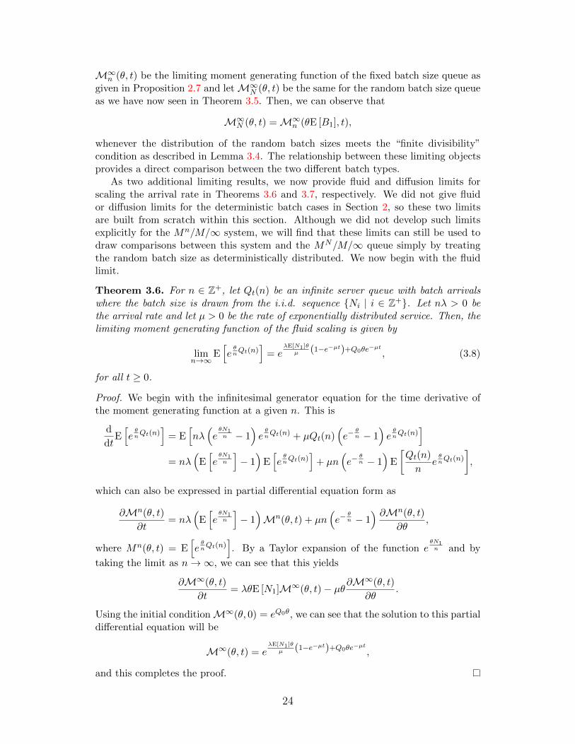
As two additional limiting results, we now provide fluid and diffusion limits forscaling the arrival rate in Theorems 3.6 and 3.7, respectively. We did not give fluidor diffusion limits for the deterministic batch cases in Section 2, so these two limitsare built from scratch within this section. Although we did not develop such limitsexplicitly for the Mn/M/∞ system, we will find that these limits can still be used todraw comparisons between this system and the MN/M/∞ queue simply by treatingthe random batch size as deterministically distributed. We now begin with the fluidlimit.

Theorem 3.6. For n ∈ Z+, let Qt(n) be an infinite server queue with batch arrivalswhere the batch size is drawn from the i.i.d. sequence {Ni | i ∈ Z+}. Let nλ > 0 bethe arrival rate and let µ > 0 be the rate of exponentially distributed service. Then, thelimiting moment generating function of the fluid scaling is given by

limn→∞

E[eθnQt(n)

]= e

λE[N1]θµ (1−e−µt)+Q0θe−µt , (3.8)

for all t ≥ 0.

Proof. We begin with the infinitesimal generator equation for the time derivative ofthe moment generating function at a given n. This is

d

dtE[eθnQt(n)

]= E

[nλ(eθN1n − 1

)eθnQt(n) + µQt(n)

(e−

θn − 1

)eθnQt(n)

]= nλ

(E[eθN1n

]− 1)

E[eθnQt(n)

]+ µn

(e−

θn − 1

)E

[Qt(n)

neθnQt(n)

],

which can also be expressed in partial differential equation form as

∂Mn(θ, t)

∂t= nλ

(E[eθN1n

]− 1)Mn(θ, t) + µn

(e−

θn − 1

) ∂Mn(θ, t)

∂θ,

where Mn(θ, t) = E[eθnQt(n)

]. By a Taylor expansion of the function e

θN1n and by

taking the limit as n→∞, we can see that this yields

∂M∞(θ, t)

∂t= λθE [N1]M∞(θ, t)− µθ∂M

∞(θ, t)

∂θ.

Using the initial conditionM∞(θ, 0) = eQ0θ, we can see that the solution to this partialdifferential equation will be

M∞(θ, t) = eλE[N1]θ

µ (1−e−µt)+Q0θe−µt ,

and this completes the proof.

24

From Corollary 3.2, we see that the mean number in system for the MN/M/∞queue is λE[N1]

µ

(1− e−µt

)+Q0e

−µt. Thus, this fluid limit moment generating function

is equivalent to eθE[Qt] for all t ≥ 0 and all θ, showing that the fluid limit convergesto the mean. We now find a connection to both the mean and the variance through adiffusion limit in Theorem 3.7.

Theorem 3.7. For n ∈ Z+, let Qt(n) be an infinite server queue with batch arrivalswhere the batch size is drawn from the i.i.d. sequence {Ni | i ∈ Z+}. Let nλ > 0 bethe arrival rate and let µ > 0 be the rate of exponentially distributed service. Then, thelimiting moment generating function of the diffusion scaling is given by

limn→∞

E

[eθ√n

(Qt(n)−nλE[N1]

µ

)]= e

λθ2

4µ (E[N1]+E[N21 ])(1−e−µt)+θQ0e−µt (3.9)

which gives a steady-state approximation of X ∼ Norm(λE[N1]µ , λ2µ

(E [N1] + E

[N2

1

])).

Proof. Through use of the infinitesimal generator, we have that the time derivative ofthe moment generating function for a given n can be expressed

d

dtE

[eθ√n

(Qt(n)−nλE[N1]

µ

)]= E

[nλ

(eθN1√n − 1

)eθ√n

(Qt(n)−nλE[N1]

µ

)+ µQt(n)

(e− θ√

n − 1)eθ√n

(Qt(n)−nλE[N1]

µ

)]= E

[√nλ

(θN1 +

θ2N21

2√n

+ O

(θ3N3

1

6n

))eθ√n

(Qt(n)−nλE[N1]

µ

)]+ E

[µ√n

(Qt(n)√

n− nλE [N1]√

nµ+nλE [N1]√

nµ

)(e− θ√

n − 1)eθ√n

(Qt(n)−nλE[N1]

µ

)],

where here we have used a Taylor expansion of the function eθN1√n . Now, forMn(θ, t) =

E

[eθ√n

(Qt(n)−nλE[N1]

µ

)], this equation can be written as a partial differential equation

as follows:

∂Mn(θ, t)

∂t= λθ

√nE [N1]Mn(θ, t) +

λθ2

2E[N2

1

]Mn(θ, t) +

√nλE

[O

(θ3N3

1

6n

)eθ√n

(Qt(n)−nλE[N1]

µ

)]+√nµ(e− θ√

n − 1) ∂Mn(θ, t)

∂θ+ nλE [N1]

(e− θ√

n − 1)Mn(θ, t).

As we take n→∞ this PDE becomes

∂M∞(θ, t)

∂t=λθ2

2E [N1]M∞(θ, t) +

λθ2

2E[N2

1

]M∞(θ, t)− µθ∂M

∞(θ, t)

∂θ,

and this yields a solution of

M∞(θ, t) = eλθ2

4µ (E[N1]+E[N21 ])(1−e−µt)+θQ0e−µt .

To observe the steady-state distribution, we take the limit as t→∞ and observe thatthis produces the moment generating function for a Gaussian.

By comparison to the limits of the expresions in Corollary 3.2 as t → ∞, we cannow observe that this steady-state approximation is equal in mean and variance to thesteady-state queue.

25

3.3 Extending the Order Statistics Sub-Systems

In Subsection 2.3 we found that the steady-state distribution of infinite server queueswith fixed batch size and general service can be written as a sum of scaled Poissonrandom variables, providing a succinct interpretation of the process and an efficientsimulation procedure for approximate calculations. The underlying observation thatsupported this approach was that we can think of an infinite server queue with batcharrivals as a collection of infinite server queues with solitary arrivals that occur simul-taneously. Using the thinning property of Poisson processes, we now extend this resultto queues with random batch sizes and general service.

Theorem 3.8. Let Qt be a MN/G/∞ queue. That is, let Qt an infinite server queuewith stationary arrival rate λ > 0, arrival batch of random size according to the i.i.d. se-quence of non-negative integer valued random variables {Ni | i ∈ Z+}, and generalservice distribution G. Then, the steady-state distribution of the number in system Q∞is

Q∞D=

∞∑n=1

n∑j=1

(n− j + 1)Yj,n (3.10)

where Yj,n ∼ Pois(λpnE

[S(j,n) − S(j−1,n)

])are independent, with S(1,n) ≤ · · · ≤ S(n,n)

as order statistics of the distribution G when Ni = n, where S(0,n) = 0 for all n andpn = P (N1 = n).

Proof. To begin, we suppose that there is somem ∈ Z+ such that P (Ni ∈ {0, . . . ,m}) =1. Then, using the thinning property of Poisson processes, we separate the arrival pro-cess into m arrival streams where the nth arrival rate is λpn. Then, by Theorem 2.11the steady-state distribution of the number in system from the nth stream is

n∑j=1

(n− j + 1)Pois(λpnE

[S(j,n) − S(j−1,n)

]).

Then, since the m thinned Poisson streams are independent, we have that the fullcombined system will be distributed as

m∑n=1

n∑j=1

(n− j + 1)Pois(λpnE

[S(j,n) − S(j−1,n)

]).

Through taking the limit as m→∞, we achieve the stated result.

We can note that Theorem 3.8 also provides a method for approximate empiricalcalculation through simulation. This representation can also be simplified if moreinformation is known about the distribution of the batch size or of the service, or both.As an example, we give the distribution for the fully Markovian system in the followingcorollary.

Corollary 3.9. Let Qt be a MN/M/∞ queue. That is, let Qt an infinite serverqueue with stationary arrival rate λ > 0, arrival batch of random size according tothe i.i.d. sequence of non-negative integer valued random variables {Ni | i ∈ Z+}, and

26

exponentially distributed service at rate µ > 0. Then, the steady-state distribution ofthe number in system Q∞ is

Q∞D=

∞∑j=1

jYj (3.11)

where Yj ∼ Pois(λjµ F̄N (j)

)are independent, where F̄N (j) = P (N1 ≥ j).

One can note that the moment generating function for this system in steady-stateis

E[eθQ∞

]= e

∑∞j=1

λjµF̄N (j)(ejθ−1),

and that this also admits a connection to the generalized Hermite distributions wediscussed in Subsection 2.2. In particular, this generalized Hermite distribution can becharacterized by λ

µ , which is again the mean of the distribution, and the complementarycumulative distribution function of the batch size distribution, which dictates the coef-ficients at each j. For this reason, it may be possible that the steady-state distributionof the queue may be simplified even further for particular batch size distributions.

Because Theorem 3.8 is again built upon an order statistics sub-queue perspective,it is natural to wonder how the distribution of the batch size would affect those sub-systems. In particular, we now consider the following scenario: suppose that the batchsize is bounded by some constant, say k, and that we have k sub-systems. For eacharriving batch, the customer with the shortest service duration will go to the first sub-system, the second shortest to the second sub-system, and so on, but only up to thenumber that have just arrived: if this batch is of size k− 1, the kth sub-queue will notreceive an arrival. In this way, the ith sub-queue represents the number in system thatwere the ith smallest in their batch. In the following proposition we find the conditionson the batch size distribution under which the distributions of the sub-queues will beequivalent.

Proposition 3.10. Consider a MB/G/∞ queueing system in which the distributionof B has support on {1, . . . , k}. Let φ ∈ [0, 1]k−1 be such that φi = P (B = i), yieldingP (B = k) = 1−

∑k−1i=1 φi. Let S(i,j) be the ith order statistics in a sample of size j from

the service distribution. Furthermore, let Qi be steady-state number in system of aninfinite server sub-queue to which the customer with the ith smallest service durationin an arriving batch will be routed whenever there are at least i customers in the batch.Let M ∈ Rk−1×k−1 be an upper triangular matrix such that

Mi,j =E[S(i,j)

]E[S(k,k)

]− E

[S(i,k)

] ,for i ≤ j and Mi,j = 0 otherwise. For v ∈ Rk−1 as the all-ones column vector, if φ issuch that

v =(M + vvT

)φ,

then QiD= Qj for all sub-queues i and j. Moreover, if 1 + vTM−1v 6= 0, then the

distributions of the sub-queues are equivalent if and only if φ = (M + vvT)−1v.

27

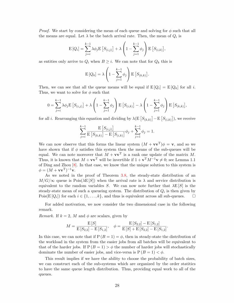
Proof. We start by considering the mean of each queue and solving for φ such that allthe means are equal. Let λ be the batch arrival rate. Then, the mean of Qi is

E [Qi] =

k−1∑j=i

λφjE[S(i,j)

]+ λ

1−k−1∑j=1

φj

E[S(i,k)

],

as entities only arrive to Qi when B ≥ i. We can note that for Qk this is

E [Qk] = λ

1−k−1∑j=1

φj

E[S(k,k)

].

Then, we can see that all the queue means will be equal if E [Qi] = E [Qk] for all i.Thus, we want to solve for φ such that

0 =k−1∑j=i

λφjE[S(i,j)

]+ λ

1−k−1∑j=1

φj

E[S(i,k)

]− λ

1−k−1∑j=1

φj

E[S(k,k)

],

for all i. Rearranging this equation and dividing by λ(E[S(k,k)

]−E

[S(i,k)

]), we receive

k−1∑j=i

E[S(i,j)

]E[S(k,k)

]− E

[S(i,k)

]φj +

k−1∑j=1

φj = 1.

We can now observe that this forms the linear system (M + vvT)φ = v, and so wehave shown that if φ satisfies this system then the means of the sub-queues will beequal. We can note moreover that M + vvT is a rank one update of the matrix M .Thus, it is known that M + vvT will be invertible if 1 + vTM−1v 6= 0; see Lemma 1.1of Ding and Zhou [8]. In that case, we know that the unique solution to this system isφ = (M + vvT)−1v.

As we noted in the proof of Theorem 3.8, the steady-state distribution of anM/G/∞ queue is Pois(λE [S]) when the arrival rate is λ and service distribution isequivalent to the random variables S. We can now note further that λE [S] is thesteady-state mean of such a queueing system. The distribution of Qi is then given byPois(E [Qi]) for each i ∈ {1, . . . , k}, and thus is equivalent across all sub-queues.

For added motivation, we now consider the two dimensional case in the followingremark.

Remark. If k = 2, M and φ are scalars, given by

M =E [S]

E [S2,2]− E [S1,2], φ =

E [S2,2]− E [S1,2]

E [S] + E [S2,2]− E [S1,2].

In this case, we can note that if P (B = 1) = φ, then in steady-state the distribution ofthe workload in the system from the easier jobs from all batches will be equivalent tothat of the harder jobs. If P (B = 1) > φ the number of harder jobs will stochasticallydominate the number of easier jobs, and vice-versa is P (B = 1) < φ.

This result implies if we have the ability to choose the probability of batch sizes,we can construct each of the sub-systems which are organized by the order statiticsto have the same queue length distribution. Thus, providing equal work to all of thequeues.

28

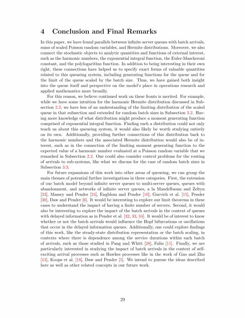
4 Conclusion and Final Remarks

In this paper, we have found parallels between infinite server queues with batch arrivals,sums of scaled Poisson random variables, and Hermite distributions. Moreover, we alsoconnect the stochastic objects to analytic quantities and functions of external interest,such as the harmonic numbers, the exponential integral function, the Euler-Mascheroniconstant, and the polylogarithm function. In addition to being interesting in their ownright, these connections have helped us to specify exact forms of valuable quantitiesrelated to this queueing system, including generating functions for the queue and forthe limit of the queue scaled by the batch size. Thus, we have gained both insightinto the queue itself and perspective on the model’s place in operations research andapplied mathematics more broadly.

For this reason, we believe continued work on these fronts is merited. For example,while we have some intuition for the harmonic Hermite distribution discussed in Sub-section 2.2, we have less of an understanding of the limiting distribution of the scaledqueue in that subsection and extended for random batch sizes in Subsection 3.2. Hav-ing more knowledge of what distribution might produce a moment generating functioncomprised of exponential integral function. Finding such a distribution could not onlyteach us about this queueing system, it would also likely be worth studying entirelyon its own. Additionally, providing further connections of this distribution back tothe harmonic numbers and the associated Hermite distribution would also be of in-terest, such as in the connection of the limiting moment generating function to theexpected value of a harmonic number evaluated at a Poisson random variable that weremarked in Subsection 2.2. One could also consider control problems for the routingof arrivals to sub-systems, like what we discuss for the case of random batch sizes inSubsection 3.3.

For future expansions of this work into other areas of queueing, we can group themain themes of potential further investigations in three categories. First, the extensionof our batch model beyond infinite server queues to multi-server queues, queues withabandonment, and networks of infinite server queues, a la Mandelbaum and Zeltyn[23], Massey and Pender [24], Engblom and Pender [10], Gurvich et al. [15], Pender[30], Daw and Pender [6]. It would be interesting to explore our limit theorems in thesecases to understand the impact of having a finite number of servers. Second, it wouldalso be interesting to explore the impact of the batch arrivals in the context of queueswith delayed information as in Pender et al. [32, 33, 34]. It would be of interest to knowwhether or not the batch arrivals would influence the Hopf bifurcations or oscillationsthat occur in the delayed information queues. Additionally, one could explore findingsof this work, like the steady-state distribution representation or the batch scaling, incontexts where there is dependence among the service durations within each batchof arrivals, such as those studied in Pang and Whitt [28], Falin [11]. Finally, we areparticularly interested in studying the impact of batch arrivals in the context of self-exciting arrival processes such as Hawkes processes like in the work of Gao and Zhu[13], Koops et al. [18], Daw and Pender [5]. We intend to pursue the ideas describedhere as well as other related concepts in our future work.

29

Acknowledgements

We acknowledge the generous support of the National Science Foundation (NSF) forJamol Pender’s Career Award CMMI # 1751975 and Andrew Daw’s NSF GraduateResearch Fellowship under grant DGE-1650441.

References

[1] Milton Abramowitz and Irene A Stegun. Handbook of mathematical functions:with formulas, graphs, and mathematical tables, volume 55. Courier Corporation,1965.

[2] Mark Brown and Sheldon M Ross. Some results for infinite server Poisson queues.Journal of Applied Probability, 6(3):604–611, 1969.

[3] Singha Chiamsiri and Michael S Leonard. A diffusion approximation for bulkqueues. Management Science, 27(10):1188–1199, 1981.

[4] Giuseppe Dattoli and HM Srivastava. A note on harmonic numbers, umbral calcu-lus and generating functions. Applied Mathematics Letters, 21(7):686–693, 2008.

[5] Andrew Daw and Jamol Pender. Queues driven by Hawkes processes. StochasticSystems, 8(3):192–229, 2018.

[6] Andrew Daw and Jamol Pender. New perspectives on the Erlang-A queue. Ad-vances in Applied Probability, 51(1), 2019.

[7] WF de Graaf, Willem RW Scheinhardt, and RJ Boucherie. Shot-noise fluid queuesand infinite-server systems with batch arrivals. Performance evaluation, 116:143–155, 2017.

[8] Jiu Ding and Aihui Zhou. Eigenvalues of rank-one updated matrices with someapplications. Applied Mathematics Letters, 20(12):1223–1226, 2007.

[9] Stephen G Eick, William A Massey, and Ward Whitt. The physics of the mt/g/∞queue. Operations Research, 41(4):731–742, 1993.

[10] Stefan Engblom and Jamol Pender. Approximations for the moments of nonsta-tionary and state dependent birth-death queues. arXiv preprint arXiv:1406.6164,2014.

[11] Gennadi Falin. The Mk/G/∞ batch arrival queue by heterogeneous dependentdemands. Journal of Applied Probability, 31(3):841–846, 1994.

[12] FG Foster. Batched queuing processes. Operations Research, 12(3):441–449, 1964.

[13] Xuefeng Gao and Lingjiong Zhu. Functional central limit theorems for stationaryHawkes processes and application to infinite-server queues. Queueing Systems,pages 1–46, 2018.

30

[14] RP Gupta and GC Jain. A generalized Hermite distribution and its properties.SIAM Journal on Applied Mathematics, 27(2):359–363, 1974.

[15] Itai Gurvich, Junfei Huang, and Avishai Mandelbaum. Excursion-based universalapproximations for the Erlang-A queue in steady-state. Mathematics of OperationsResearch, 39(2):325–373, 2013.

[16] CD Kemp and Adrienne W Kemp. Some properties of the ‘Hermite’ distribution.Biometrika, 52(3-4):381–394, 1965.

[17] Donald E Knuth. Johann Faulhaber and sums of powers. Mathematics of Com-putation, 61(203):277–294, 1993.

[18] DT Koops, M Saxena, OJ Boxma, and M Mandjes. Infinite-server queues withHawkes input. Journal of Applied Probability, 55(3):920–943, 2018.

[19] Soon Seok Lee, Ho Woo Lee, Seung Hyun Yoon, and Kyung C Chae. Batch arrivalqueue with N-policy and single vacation. Computers & Operations Research, 22(2):173–189, 1995.

[20] Liming Liu and James GC Templeton. Autocorrelations in infinite server batcharrival queues. Queueing Systems, 14(3-4):313–337, 1993.

[21] Yi Lu, Qiaomin Xie, Gabriel Kliot, Alan Geller, James R Larus, and AlbertGreenberg. Join-idle-queue: A novel load balancing algorithm for dynamicallyscalable web services. Performance Evaluation, 68(11):1056–1071, 2011.

[22] David M Lucantoni. New results on the single server queue with a batch Markovianarrival process. Communications in Statistics. Stochastic Models, 7(1):1–46, 1991.

[23] Avishai Mandelbaum and Sergey Zeltyn. Service engineering in action: thePalm/Erlang-A queue, with applications to call centers. In Advances in servicesinnovations, pages 17–45. Springer, 2007.

[24] William A Massey and Jamol Pender. Gaussian skewness approximation for dy-namic rate multi-server queues with abandonment. Queueing Systems, 75(2-4):243–277, 2013.

[25] Hiroyuki Masuyama and Tetsuya Takine. Analysis of an infinite-server queue withbatch Markovian arrival streams. Queueing Systems, 42(3):269–296, 2002.

[26] Rupert G Miller Jr. A contribution to the theory of bulk queues. Journal of theRoyal Statistical Society. Series B (Methodological), pages 320–337, 1959.

[27] Robin Kingsley Milne and Mark Westcott. Generalized multivariate Hermite dis-tributions and related point processes. Annals of the Institute of Statistical Math-ematics, 45(2):367–381, 1993.

[28] Guodong Pang and Ward Whitt. Infinite-server queues with batch arrivals and de-pendent service times. Probability in the Engineering and Informational Sciences,26(2):197–220, 2012.

31

[29] Jamol Pender. Poisson and Gaussian approximations for multi-server queues withbatch arrivals and batch abandonment. 2013.

[30] Jamol Pender. Gram Charlier expansion for time varying multiserver queues withabandonment. SIAM Journal on Applied Mathematics, 74(4):1238–1265, 2014.

[31] Jamol Pender and Tuan Phung-Duc. A law of large numbers for M/M/c/delayoff-setup queues with nonstationary arrivals. In International Conference on Analyti-cal and Stochastic Modeling Techniques and Applications, pages 253–268. Springer,2016.

[32] Jamol Pender, Richard H Rand, and Elizabeth Wesson. Queues with choice viadelay differential equations. International Journal of Bifurcation and Chaos, 27(04):1730016, 2017.

[33] Jamol Pender, Richard H Rand, and Elizabeth Wesson. Strong approximationsfor queues with customer choice and constant delays. 2017.

[34] Jamol Pender, Richard H Rand, and Elizabeth Wesson. An analysis of queueswith delayed information and time-varying arrival rates. Nonlinear Dynamics, 91(4):2411–2427, 2018.

[35] Rainer K Sachs, Pei-Li Chen, Philip J Hahnfeldt, and Lynn R Hlatky. DNAdamage caused by ionizing radiation. Mathematical biosciences, 112(2):271–303,1992.

[36] DN Shanbhag. On infinite server queues with batch arrivals. Journal of AppliedProbability, 3(1):274–279, 1966.

[37] Hideaki Takagi and Yoshitaka Takahashi. Priority queues with batch Poissonarrivals. Operations Research Letters, 10(4):225–232, 1991.

[38] Qiaomin Xie, Mayank Pundir, Yi Lu, Cristina L Abad, and Roy H Camp-bell. Pandas: Robust locality-aware scheduling with stochastic delay optimality.IEEE/ACM Transactions on Networking (TON), 25(2):662–675, 2017.

[39] Ali Yekkehkhany, Avesta Hojjati, and Mohammad H Hajiesmaili. GB-PANDAS::Throughput and heavy-traffic optimality analysis for affinity scheduling. ACMSIGMETRICS Performance Evaluation Review, 45(2):2–14, 2018.

32