Lappeenrannan teknillinen yliopisto Lappeenranta University of Technology

Tuomo Lindh

ON THE CONDITION MONITORING OF INDUCTION MACHINES

Thesis for the degree of Doctor of Sci-ence (Technology) to be presented with due permission for public exami-nation and criticism in the auditorium 1382 at Lappeenranta University of Technology, Lappeenranta, Finland on the 13th of December, 2003, at noon.

Acta Universitatis Lappeenrantaensis 174

ISBN 951-764--841-3 ISBN 951-764--843-X (PDF)

ISSN 1456-4491

Lappeenrannan teknillinen yliopisto Digipaino 2003

Abstract Tuomo Lindh Lappeenranta University of Technology Acta Universitatis Lappeenrantaensis 174 On the Condition Monitoring of Induction machines Lappeenranta 2003 ISBN 951-764-841-3, ISSN 1456-4491 ISBN 951-764--843-X (PDF) The research of condition monitoring of electric motors has been wide for several decades. The research and development at universities and in industry has provided means for the predictive condition monitoring. Many different devices and systems are developed and are widely used in industry, transportation and in civil engineering. In addition, many methods are developed and reported in scientific arenas in order to improve existing methods for the automatic analysis of faults. The methods, however, are not widely used as a part of condition monitoring systems. The main reasons are, firstly, that many methods are presented in scientific papers but their performance in different conditions is not evaluated, secondly, the methods include parameters that are so case specific that the implementation of a system using such methods would be far from straightforward. In this thesis, some of these methods are evaluated theoretically and tested with simulations and with a drive in a laboratory. A new automatic analysis method for the bearing fault detection is introduced. In the first part of this work the generation of the bearing fault originating signal is explained and its influence into the stator current is concerned with qualitative and quantitative estimation. The verification of the feasibility of the stator current measurement as a bearing fault indicator is experimentally tested with the running 15 kW induction motor.

The second part of this work concentrates on the bearing fault analysis using the vibration measurement signal. The performance of the micromachined silicon accelerometer chip in con-junction with the envelope spectrum analysis of the cyclic bearing fault is experimentally tested. Furthermore, different methods for the creation of feature extractors for the bearing fault classi-fication are researched and an automatic fault classifier using multivariate statistical discrimination and fuzzy logic is introduced. It is often important that the on-line condition monitoring system is integrated with the industrial communications infrastructure. Two types of a sensor solutions are tested in the thesis: the first one is a sensor with calculation capacity for example for the production of the envelope spectra; the other one can collect the measurement data in memory and another device can read the data via field bus. The data communications requirements highly depend on the type of the sensor solution selected. If the data is already analysed in the sensor the data communications are needed only for the results but in the other case, all measurement data need to be transferred. The complexity of the classification method can be great if the data is analysed at the management level computer, but if the analysis is made in sensor itself, the analyses must be simple due to the restricted calculation and memory capacity. Keywords: condition monitoring, electric motor, fault classification, bearing fault, bearing damage UDC 004.7 : 658.588.1 : 621.313.33

Acknowledgements This research work has been carried out during years 2000-2003 in the laboratory of Electric Power Systems in Lappeenranta University of Technology. The work has been done under a technology program Tesla (1998-2002) and a its sub-project “Management of Electrical Sys-tems in Industrial Plants”. The research has been mainly financed by the Technology Development Centre Tekes and ABB Oy. I would like to thank all the people that are participated in the preparation of this thesis. Espe-cially, I wish to thank the supervisor of this thesis, professor Jarmo Partanen, for giving me the opportunity to carry out this thesis and for his interest in my research work. I would also like to thank my colleague M. Sc. Jero Ahola for a good co-operation and for his valuable ideas that have helped me greatly during the research. Additionally, I wish to thank the whole research group Petr Spatenka, Anna-Lena Rautiainen, Risto Tiainen and Ville Särkimäki as well as D. Sc. Joni-Kristian Kämäräinen and D. Sc. Ville Kyrki for the valuable co-operation. I wish to thank professor Juha Pyrhönen for his comments and help in measurements. I also thank D. Sc. Markku Niemelä for his comments, suggestions and helping me several times in practical arrangements concerning electric motors and electrical drives. I wish also thank D. Sc. Janne Nerg for FEM-computation. I would like to thank the pre-examiners of this doctoral thesis, professor Tapani Jokinen and professor Jan Rusek for their valuable comments and corrections. Financial support by Suomen kulttuurirahaston Etelä-Karjalan rahasto and Lahja ja Lauri Hoti-sen rahasto is greatly appreciated. Lappeenranta, November the 15th, 2003 Tuomo Lindh

CONTENTS

Abstract

Acknowledgement

Contents

Abbreviations and Symbols

1. INTRODUCTION......................................................................................................................15

1.1 Background and motivation.........................................................................................15

1.2 Objectives of the study.................................................................................................17

1.3 The structure of the thesis ............................................................................................18

1.4 Scientific contribution of the thesis .............................................................................19

2. CONDITION MONITORING PROCEDURES AND MAIN DAMAGE TYPES OF INDUCTION MOTORS ............................................................................................................21

2.1 Condition monitoring procedures ................................................................................21

2.1.1 Periodical or continuous condition monitoring? ...........................................21

2.1.2 Condition monitoring measurements and techniques....................................22

2.1.3 Analysis methods ..........................................................................................23

2.2 Main damage types of induction motors......................................................................25

2.3 Vibration, stator current and temperature; Condition measurements concerned in the thesis ......................................................................................................................29

3. THEORY OF BEARING DEFECT DETECTION....................................................................31

3.1 Vibration ......................................................................................................................31

3.1.1 Characteristic frequencies due to bearing failures and measured vibration signal .............................................................................................................32

3.1.2 Envelope spectrum of the vibration signal ....................................................36

3.2 Rotor eccentricity and unbalanced magnetic pull (UMP)............................................38

3.3 Behaviour of stator current due to bearing fault ..........................................................44

3.4 Conclusions..................................................................................................................46

4. METHODS FOR ANALYSIS OF A NON-STATIONARY SIGNAL......................................47

4.1.1 Time-frequency analysis ...............................................................................48

4.1.2 Statistical signal classification using Mahalanobis distance .........................51

4.1.3 Method of Yazici...........................................................................................54

4.1.4 Optimal Gabor filter parameter selection for classification ..........................55

4.2 Conclusions..................................................................................................................57

5. TESTING EQUIPMENT ...........................................................................................................58

6. TESTS FOR THE DETECTION OF A BEARING FAULT USING STATOR CURRENT MEASUREMENTS ...................................................................................................................62

6.1 Change of air gap in a DC-magnetised induction motor..............................................62

6.2 Methods using frequency spectrum of the stator current .............................................66

6.2.1 Averaged power spectra of a stator current signal ........................................66

6.2.2 Classification of power spectra of stator current signals using Mahalanobis distance calculation .......................................................................................67

6.2.3 Simulation of STFT and the Mahalanobis distance calculation with a test signal .............................................................................................................70

6.2.4 Experimental test results using STFT and the Mahalanobis calculation .......75

6.2.5 The optimisation of the time-frequency window for a detection of the bearing fault using a stator current signal......................................................91

6.3 Conclusions..................................................................................................................95

7. MICROMACHINED SILICON ACCELEROMETER .............................................................97

7.1 Characteristics of conventional piezoelectric sensors and micromachined sensors.....97

7.2 Measurement apparatus ...............................................................................................99

7.3 Measurements ............................................................................................................100

7.3.1 Envelope spectra at no load.........................................................................102

7.4 Envelope spectra at full load......................................................................................103

7.5 Conclusions................................................................................................................108

8. AUTOMATIC ANALYSIS OF AN ACCELERATION SIGNAL..........................................109

8.1 Feature extraction ......................................................................................................109

8.1.1 Autocorrelation of a time-frequency presentation of a signal .....................109

8.1.2 Envelope autocorrelation method................................................................111

8.1.3 Envelope detectors for the envelope spectrum method ...............................113

8.1.4 Conclusions concerning the feature extractors............................................117

8.2 Classification of features............................................................................................118

8.2.1 Classification using the Mahalanobis distance calculation and minimum distance classifier ........................................................................................118

8.2.2 Classification using fuzzy logic ..................................................................122

8.2.3 Conclusions concerning the fault classification ..........................................126

8.3 Embedded and remote analysis..................................................................................126

8.3.1 DSP based testing platform .........................................................................127

8.3.2 Remote analysis based testing platform ......................................................130

8.3.3 Management level connection.....................................................................133

8.3.4 Conclusions concerning embedded and remote analysis.............................134

8.4 Conclusions concerning the automatic analysis of the acceleration signal ................135

9. SUMMARY AND CONCLUSIONS.......................................................................................136

9.1 Key results of the thesis .............................................................................................136

9.2 Conclusions................................................................................................................138

References ………………….….…..……………………………………………………………140

ABBREVIATIONS AND SYMBOLS

Letters

α Angle, area, parameter A amplitude B,b flux density c covariance C capacitance C class d,D diameter, diameter of rolling element, dimension, distance D diameter, pitch diameter, dimension δ Dirac’s delta function, nominal airgap length E energy ε eccentricity f frequency fb characteristic frequency of rolling element fault, bearing pass frequency of

rolling element fi characteristic frequency of inner race fault, bearing pass frequency of inner race fib frequency of bearing vibration modulated in current fo characteristic frequency of outer race fault, bearing pass frequency of outer race fr rotational frequency of rotor fc characteristic frequency of cage fault, bearing pass frequency cage fault fvb frequency of bearing vibration F F- distribution Fs sampling frequency Φ cumulative normal distribution g airgap length, gaussian distribution h,H system i,I current j,J current density γ duration and bandwidth parameter l length L inductance λ noncentrality parameter Λ permeance k number µ mean µ0 permeability of air m mean N number, number of rolling elements n rotational speed, discrete time index r radius, distance R resistance Rm reluctance S distance S set σ standard deviation ρ resistivity t,τ time

u,U voltage Θ magnetomotive force (MMF), ampere turns ϖ , Ω angular velocity x signal xl linear distance along air gap circumference

i current space vector m mean vector C covariance matrix F feature vector u voltage space vector Ψ flux linkage

Subscripts

a axle b ball, broken be bearing impulse c housing, cage, case h healthy i inner l learning, training m modulating,magnetising me measured nm non-modulating o outer, output r rotor s stator, subset σ leakage t test, transient tp transfer path Superscripts g arbitrary frame s stator frame ^ peak value, Fourier- domain, Hilbert transformed * complex conjugate Acronyms AAF anti-aliasing filter AD, A/D analog-digital (conversion) ANN artificial neural network CPLD complex programmable logic device CR critical value (for 95%, 99% confidence level) DC direct current DMA direct memory access DSP digital signal processor EMF electromotive force

FDR Fisher’s discrimination ratio FEM finite element method FIR finite impulse response FFT fast Fourier transform GPRS general packet radio service IIR infinite impulse response ISO international organization for standardization MEMS micromachined electromechanical system MLP multi layer perceptron MMF magnetomotive force MUX multiplexer PSD power spectral density RMS root mean square RTU remote terminal unit SNR signal to noise ratio SPI serial peripheral interface SOM self organising map SDRAM synchronous dynamic random access memory SRAM static random access memory STFT short-time Fourier-transform OER optimum error ratio OVL overlapping coefficients UMP unbalanced magnetic pull WT wavelet transform WVT Wigner-Ville transform

15

1. INTRODUCTION

1.1 Background and motivation

The maintenance relies on the statistical life estimation or on the predictive condition monitor-ing. Even the run-to-failure strategy can be selected. The selection between the strategies is normally based on economical or security factors. The sum of all maintenance costs such as production losses, repair costs, new components and the condition monitoring costs should be minimised.

The statistical life estimation is based on the experimental knowledge of the behaviour of the aging component. It can take into account many ambient factors such as the loading rate and the operating temperature but there remain many unpredictable factors that can lead to failure with-out condition monitoring.

The predictive condition monitoring of electrical motors means continuous or periodical evalua-tion of the healthiness of the motor. As a result of this evaluation an estimate of reliable lifetime is achieved if the tested motor is broken or healthy is determined. The first goal seems to be more difficult with an estimated grade of deterioration but in fact the latter goal is often the most difficult to achieve. In order to divide the condition of the motor between broken or healthy the grade of deterioration is evaluated and the degree of deterioration that indicates the broken condition is determined. If the limit is too high, the risk of shut-down of process is big. If the limit is too low, the change or repair of the motor is often supposed to be unnecessary and in fact the possibility of incorrect determination is high.

The main objective of the condition monitoring is to alarm against future damage if no action is taken. This is the main difference between condition monitoring and protection of the motors which prevents additional damage to the motor but also often causes very high economical losses caused by the shut-down of the production process.

Electric motors are often considered to be very reliable, which means that investment in on-line condition monitoring as a separate system is often not economically justified. On the other hand, many researches indicate, that broken motors account for significant fraction of losses caused by shutdown times of industrial processes. This has been made in a research (Lem-piäinen, 1995) in Kaukopää paper factory of StoraEnso. During that research less than 40 % of all faults were due to electrical systems. Motors represented 24 % of the total shutdown time due to electrical system faults. This is illustrated in Figure 1-1. The number of failures of elec-tric motors is smaller than its relative portion of the total shut-down time because of the longer replacement/clearing time than of many process automation faults, sensor damages and supply faults.

16

Cable10 %

Motor , generator24 %

Protection device5 %Process automation

23 %

Sensor12 %

Electric supply4 %

Contactor, circuit breaker4 %

Others18 %

Fig. 1-1 Relative total shutdown times caused by electric systems in paper factory of Enso in Kaukopää (Lempiäinen, 1995).

There exists many systems for condition monitoring of industrial processes, especially of rotat-ing machinery. The condition monitoring usually covers the electric motors that are driving the monitored processes. There are on-line systems designed mainly for condition monitoring of electric motors, too. These systems usually consist of a measuring and data processing device, which can be connected permanently to a data bus supplying information to a analysing com-puter or data can be collected from the device occasionally. A selection between continuous data transfer and manually performed data collection is made mainly on the cost of instrumenta-tion and labour. On the other hand, a modern industrial infrastructure includes communications buses at all level from actuator level (field level) to management level. Recently, the industrial infrastructure is further widened with tools that make it possible to manage industrial systems globally through Internet (Ahola, 2000), (Lindh, 2001). The alternative means for the connec-tions are presented in Fig. 1-2. Therefore, using existing communication buses, it is often possible to transfer data between the global management level and the condition monitoring device connected to the field level bus.

17

M

M

BININ/OUT

FBCOMM.

Process Unit Process Unit

PROCESS BUS

Control Room

ProcessStation

FBCOMM.

FBCOMM.

I/O BUS

Local Area Network (Ethernet)

InformationCenter

DatabaseServer

DatabaseServer

Data Acquisitionand ManagementSystem for ManagementApplicationsof Industrial ElectricalSystems

PMU

Energy ManagementSystem

DatabaseServer

ProcessStation

ProcessStation

ProcessStation

ProcessStation

PLCPLCPLC

FIELDBUSField Level

ProcessControlLevel

ManagementLevel

OPC -Server

FIELDBUS

ElectricalSystemsManagement Application

Office Workstation

Local Area Network (Ethernet)

DatabaseServer

Outsourced servicesof expert organisations

GlobalManagementLevel

INTERNET

WAN

Field Level

Local Area Network (Ethernet)

DatabaseServer

Outsourced servicesof expert organisations

GlobalManagementLevel

INTERNET

WAN

fielddevice

application

web-pages

TCP-IPhttp

ManagementLevel

LAN

Local Area Network (Ethernet)

DatabaseServer

servicesin intranet

fielddevice

application

web-pages

TCP-IPhttp

fielddevice

application

web-pages

TCP-IPhttp

Fig. 1-2. Traditional industrial information infrastructure model extended with a global management level (left). The infrastructure model on the right side provides direct field level access from the global management level.

The outsourcing of the production, service and maintenance is a growing trend. Companies try to concentrate on their core business and leave all the business supporting tasks to other compa-nies that are specialised in those areas. As a small consequence of that, service companies are often responsible for the maintenance and condition monitoring of electrical equipment. The management of electric distribution may be the responsibility of another company and so on. Many new functions become possible as the outsourced service becomes based on Web-based technology, e.g. power quality monitoring. In order to cost-efficiently supervise and control devices at different levels of the industrial infrastructure model, data communication between supervisor and the target device is needed.

1.2 Objectives of the study

The primary goal of this thesis is the evaluation of methods that can be used in order to con-

struct automatic condition analysis tools for the detection of bearing faults in induction motors.

18

Bearings are of prime concern in condition monitoring of rotating machinery including electri-cal motors. On the other hand, a stator current measurement has an important role in the condition monitoring of induction motors. Unbalanced rotor, rotor bar damages, damaged stator windings can be indicated by analyses based on the stator current measurement. The stator current measurement would be sufficient as the only condition monitoring “sensor” if the bear-ing damages were found by analyses based on this measurement. Many promising papers presenting methods that could be used for indication of these faults by use of a stator current measurement have been published (Schoen, 1995), (Penman, 1994), (Yazici, 1997).

On the other hand, vibration monitoring is required if the stator current measurement cannot provide information needed for the detection of bearing faults. The vibration monitoring de-vices must be fixed to a motor frame. An economical means for constructing vibration monitoring as a part of condition monitoring concept is surveyed. The vibration measurement based on micromachined silicon accelerometers combined with embedded processing and data communications is studied.

In order to implement an on-line condition monitoring system or concept in an industrial envi-ronment as economically as possible, it is required that communication possibilities of the industrial environment are utilised. Depending on the solution selected, the analyses of condi-tion are performed in a measuring device, power controlling devices such as switches, frequency converters etc. or in computers at local or global management level in industrial plants (Lindh, 2001), (Lindh, 2002e). If all analyses are made in measuring devices, the big processing capacity of the device is required. If the measurement device only collects data, calculation capacity requirements are more modest but the capacity of communication is ex-tended. This is due to the necessity of transferring measurement data (perhaps pre-processed) to an analysing device. It is possible that vibration monitoring is needed in order to achieve ade-quate reliability of the condition estimate of the induction motor. In this case, the data must be transferred from the motor installation place. One objective of this thesis is to demonstrate these possibilities when condition monitoring is implemented with a stand- alone condition monitor-ing device or as a part of some other devices such as the motor protection relay. The implementation of the condition monitoring device should adapt to the industrial information infrastructure providing means for global monitoring.

1.3 The structure of the thesis

The contents are divided in 9 chapters. Besides this introductory chapter, the following chapters are presented:

Chapter 2 presents the condition monitoring procedures generally and lists possible techniques that indicate the condition of motors. It also deals with aims and the requirements set for the condition monitoring systems. It also presents dependences between different measurements and indication of faults as well as dealing with analysis methods and approaches that can be used.

It also introduces the main damage types of induction motor. The purpose is to show the impor-tance of the bearing defects among other defects and to explain the deterioration and faulting mechanisms of rolling element bearings.

Chapter 3 deals with the bearing defect detection. Firstly, the generation of the bearing fault originating vibration signal is explained, secondly an analysis with an envelope spectrum method is explained. The effects of rotor eccentricity are discussed. The rotor eccentricity due

19

to bearing fault can induce stator current transient. This phenomenon is explained with a space vector model for the induction motor.

Chapter 4 presents methods for the analysis of non-stationary signals. Possible methods that can reveal tiny stator current transients are discussed. The basic schema of the pattern classification is presented and statistical discrimination of multivariate data using Mahalanobis distance calculation is explained.

Chapter 5 describes the testing arrangements and equipment used in the tests of the following chapters.

Chapter 6 presents the experimental verification of the feasibility of the motor bearing damage detection using stator current monitoring. A success of the correct detection depends on the motor structure and bearing type (internal radial clearance of the bearing).

Chapter 7 discusses the possibilities and restrictions of micromachined silicon accelerometers as bearing fault detectors. Experimental results using the envelope spectrum method are pre-sented.

Chapter 8 introduces analysis methods for automatic bearing fault detection. The methods are tested with real-time devices. The requirements of different on-line detection solutions are dis-cussed in terms of memory requirements, complexity of calculations and data transfer requirements.

Chapter 9 concludes the thesis and gives some suggestions for future work.

1.4 Scientific contribution of the thesis

If the most usual bearing faults could be diagnosed with the stator current measurement based analyses, no other measurements would be needed in order to cover all of the most important failure types of an induction motor. In this thesis the existence of a stator current transient due to the radial movement of the rotor is to be theoretically proved and the magnitude of such a transient will be approximately evaluated. Further, the evaluation will be verified with a DC-current magnetisation test, in which, radial shocks are applied to the rotor and a radial dis-placement, an acceleration level and a stator current transient is measured. The stator current transient due to a bearing fault will be estimated to be maximally in the class of tens of milli-amperes and typically a few milliamperes. The verification of the feasibility of the stator current measurement as a bearing fault indicator will be experimentally tested with a running 15 kW induction motor. It will be shown that the stator current measurement as a bearing fault indica-tor is not adequate in a case of a 15 kW 4-pole motor with a bearing with normal internal radial clearance. Therefore, the feasibility of the stator current measurement as a bearing fault indica-tor is questionable in practical condition monitoring where a high reliability of analysis is required.

While the stator current measurement based bearing fault diagnosis is found unreliable in prac-tical condition monitoring the means to construct low cost bearing monitoring systems using motor frame acceleration measurement are required. The micromachined accelerometers are one alternative to traditional piezo-electric sensors. The characteristics of traditional piezoelec-tric sensors and capacitive micromachined sensors will be presented and the effects of features and performance limitations on condition monitoring of the bearings of the electric motors will

20

be discussed. The detection of the most incipient faults (frame response <10mg) that can be found using the piezoelectric sensor is not possible due to the bigger noise level of micro-machined accelerometer. On the other hand, if the dominant vibration is big the amplitude range of the micromachined accelerometer is not adequate. However, the micromachined sensor chips can be used in condition monitoring of the bearings in most motor drive environments.

In this thesis, guidelines for the automatic detection of bearing faults will be given and two different schemas for a condition monitoring system will be presented. Both schemas imple-ment a system integrated with industrial information infrastructure.

The automatic fault analysis consists of the feature extraction and the fault classification. Dif-ferent feature extraction methods will be tested. The guidelines for statistical fault classification using Mahalanobis- distance and deterministic classification with multi valued fuzzy logic and a combination of these will be presented. Based on the tests, the automatic classification using the envelope spectra of frame vibration is possible. However, due to the rather limited test data, the results remain quite case specific.

21

2. CONDITION MONITORING PROCEDURES AND MAIN DAMAGE TYPES OF INDUCTION MOTORS

In this chapter the condition monitoring procedures are discussed. Advantages of periodical and continuous monitoring are presented. Common failure mechanisms of the motors as well as failure mechanisms of the bearings are presented. The chapter generally describes the methods and the measures that can be used in condition monitoring of different faults in motors.

2.1 Condition monitoring procedures

The maintenance can be corrective (reactive, run-to-failure) which means that broken compo-nents are replaced or repaired. The use of corrective maintenance leads to low reliability if the establishment includes many possible damaging objects. Unplanned downtime and possible breakdown of other devices, than primarily broken components, can make reactive maintenance very expensive. Preventive maintenance with scheduled service procedures can prevent typical damages. For example, if the majority of bearings exceed their expected lifetime (when lubri-cated between the correct lubrication intervals), the preventive maintenance can prevent most of the bearing damages by changing bearings before the expected lifetime expires. On the other hand, if the expected lifetime cannot be determined (deterioration expectations are not known e.g. in the case of rotor faults) the scheduled maintenance is relatively inefficient. The predic-tive maintenance means condition based actions. These require condition monitoring in order to detect deterioration. The proactive maintenance tries to improve the object (process) so that the probability of the damage is decreased in the future. This type of maintenance is not natural in the case of electric motor maintenance.

2.1.1 Periodical or continuous condition monitoring?

The condition monitoring is often divided into off-line and on-line monitoring. In the case of the off-line monitoring: the monitored object is not in a running state while monitoring actions are made. The on-line monitoring is applied to the running objects meaning that normal produc-tion process can continue during monitoring.

Further, the condition monitoring can be divided into periodical and continuous. The periodical condition monitoring can be off-line or on-line monitoring but the continuous monitoring is usually made on-line. Furthermore, the off-line monitoring can be invasive which means that the motor structure must be disassembled for monitoring. On the contrary, the on-line monitor-ing is almost always non-invasive. The continuous on-line monitoring is based on measurements. Periodical monitoring is made manually and can include also evaluation based on human senses. Human can notice marks of poor condition that cannot be found with con-tinuous on-line monitoring. Such marks of poor condition (or of a condition that can lead to failure) include a degree of dirtiness, abnormal colour or acoustic noise. The advantages of continuous condition monitoring include:

• Damages can be detected as soon as they appear. • Trends can be formed automatically. • Minimum need for labour. • Detection of sudden changes is possible. • Motors that are difficult to reach by a man can be easily monitored.

22

The advantages of periodical condition monitoring include: • Motors can be cleaned from dust or other particles when measurements are done. • Humans can discover changes in appearance such as mechanical damages, leaking

seals, loosened fastenings etc. • Investment for condition monitoring is smaller than in continuous condition monitor-

ing systems.

In the most usual case, continuous condition monitoring of motors is applied as part of a proc-ess condition system. In such a case, the monitoring covers electric motors that are connected to the monitored processes. There are continuous on-line systems designed mainly for condition monitoring of electric motors, too. These systems usually consist of a measuring and data proc-essing device, which can be connected permanently to a data bus supplying information to the analysing computer or data can be collected from the device occasionally. The selection be-tween continuous data transfer and manually performed data collection is made mainly on the costs of instrumentation and labour.

2.1.2 Condition monitoring measurements and techniques

If the condition monitoring of an electric motor is based on measurements there are two ways to indicate alarm level for deterioration. The first one is the use of alarm limits on a measured or analysed quantity and the other is the change in the long-term trend of measurements which indicates change in the motor or drive. Measurements can be analysed in time- or frequency domain or in combination of these (time-frequency analysis).

Possible measured quantities and techniques that indicate the condition of an electric motor are numerous: • electrical and magnetic techniques

• stator current • electrical or mechanical torque, power • axial flux, stray flux of winding end, air gap flux

• vibration, noise • velocity or acceleration measurement • measurement of acoustic noise pressure

• measurement of displacement of rotor • temperature

• temperature measurements with thermocouples, thermistors etc. • temperature images

• chemical analysis • gas analysis of ventilation air • particle analysis of ventilation air

• visual inspection • rotational velocity changes • partial discharge

On-line condition monitoring can utilise all of the listed techniques. However, some of these techniques require expensive devices and are therefore used mostly for the monitoring of big generators (partial discharge, gas analysis etc.). In addition, some methods require installation that can be made only when the motor is disassembled. For example, an air gap flux measure-ment requires a sensor in the air gap but the axial flux can be measured outside the motor frame (Kokko, 2003).

23

In the case of a condition monitoring system with on-line data collection, indication and an analysis of the electric motor faults often requires locally made calculations in embedded sys-tems as well as analysis tools running in separate computers at the management level (see figure 1-2). High frequency data of electric, magnetic or mechanic quantities have to be calculated locally in order to avoid the need for a high capacity field bus at the device level. Many compli-cated tasks can be done in embedded systems such as transformation to the frequency domain, adaptive filtering or fuzzy reasoning. On the other hand, indications of certain faults are reliable only with very complicated analysis or when results are compared to previous results of a long period of time.

The devices used in controlling and protection of the motors and drives include a very different number and quality of measurements, data processing capacity and communications capacity. During this research, however, it was found that most of these devices could include some con-dition monitoring functions besides their primary use. The construction of a condition monitoring concept for these devices is a challenging task if it is required, that the concept ful-fils most of the following requirements:

• economically reasonable • uses existing measurements • algorithms are adapted to the processing capacity of the device • uses existing data transfer possibilities • can work as a part of an existing condition monitoring system • indicate failures reliably and makes no false alarms • is tolerant to different ambient factors • uses information of external sources through communications bus • requires no/little human work in condition analyses.

2.1.3 Analysis methods

Analysis methods used in the condition monitoring of electric motors are numerous. The meth-ods can be divided into deterministic and non-deterministic methods (Partanen, 1999). Deterministic, in this case, means that the physical characters of the object determines the con-dition estimate with the aid of heuristics and calculations directly. Deterministic methods include parameter estimation, rule-based methods, fuzzy-logic and mathematical modelling. Non-deterministic, in this case, means that a significant degree of contingency or unknown determining factors exist. Therefore, the measured quantity does not determine the condition directly. Non-deterministic (or stochastic) methods include probability distributions and artifi-cial neural networks. Non-deterministic methods often use statistical pattern classification for decision-making. On the other hand, a condition analysis procedure often includes both types of analyses. Often, based on some deterministic model, the values describing the condition are formed. These values are then post processed with non-deterministic methods e.g. in the paper of Kyusung (2002).

Purely a deterministic approach based on known machine parameters, parameter estimation, physical characters and operational values is suitable for indication of faults that have a definite limit to distinguish faulty and healthy conditions. This is possible especially in cases, where the measurement is closely connected to physical phenomenon or an indication is based on esti-mated values and a mathematical model (e.g. motor model). A temperature measurement and an overheat limit is the most straightforward example of this kind of the indication. A bearing fault indicated from vibration also belongs to this category. A purely deterministic approach

24

becomes difficult if indication of incipient faults has to be automated. A visual inspection of spectrum components can reveal a fault that cannot be given by deterministic limits or equa-tions.

Statistical methods are often used in order to indicate faults. Statistical analysis is made on the measured quantity directly or to the quantity derived from measures. The use of the statistical analysis using an artificial neural network (ANN) has been demonstrated e.g. in the paper of Chow (1984) in which a neural network indication of bearing fault is presented. Rotational speed and stator current were measured and faults were educated to ANN. Schoen (1994a) has used ANN and the stator current measurement in order to indicate rotor eccentricity and bearing cage deformation. Paya and Esat (1997) have used ANN in the bearing and gear box fault diag-nostics using Wavelets in order to pre –process the vibration signal. The main difficulties of ANN are that educational data are case specific and other factors than faults can cause condi-tions that indicate faults. A comparison between the deterministic autoregressive modelling technique and the ANN –technique is made in research of Baillie (1996). Other statistical meth-ods that are used in condition monitoring include clustering of data (Penman, 1994), statistical discriminant analysis and Hidden Markov models (Ocak, 2001), for example.

A time-frequency analysis can be used when the changes in measured quantities are small and time variant. This is a normal situation in the case of very incipient faults or when the meas-ured quantity is weakly linked to fault. The time-frequency transformation is most often made with Short-Time Fourier Transform (STFT) or with Wavelet Transform (WT). The indication of faults in time-frequency analysis can be automated by using for example, Multi Layer Per-ceptron (MLP) neural network or statistical pattern recognition methods such as discriminant analysis or self- organising maps (SOM). If MLP ANN method is used, faulty and healthy situations have to be trained to a network. The measured and transformed data is fed to the network and the output is the condition information. The selection and the amount of training data determines the feasibility of the method.

Both supervised and unsupervised ANN methods have been used for the pattern recognition of motor faults (Penman, 1994), (Yin, 1995). Unlike supervised ANN, the unsupervised ANN can classify features without supervision but a correspondence of a certain feature and fault has to be determined. The output is changed because of the fault but a reason for the change cannot be determined without previous examples about faulty situation. From the results of ANN, inverse problem solving is not possible.

Fuzzy logic. A neural network can provide the correct input-output fault detection relation, but it is a “black-box” that does not provide any heuristic reasoning (Chow, 1997). Therefore, it cannot explain the faults. ANN is often case sensitive and therefore, is not adequate as an only fault indicator. Fuzzy-logic, instead, is based on heuristic reasoning. It can handle the concept of partial truth, the truth values between zero and one. Also, the output information is multi-valued. Therefore, in the area of condition analysis, the fuzzy logic can output the degree of the fault, the “probability” of the fault or give many parallel suggestions for further analysis. The linguistic, heuristic and any other type of input information are used to form subsets (condi-tions) such as “low vibration level” and “high vibration level” that can overlap. These are called membership functions. The membership functions are processed with fuzzy rules (IF -THEN statements) in order to form memberships in output sets (the degrees of output conditions). The output sets are often defuzzified; the sets are changed to a crisp number with a calculation that weights the conditions to a large degree (probability). Fuzzy logic has been used in the condi-tion monitoring analyses by e.g. Mechefske (1998) and Benbouzid (2001). Mechefske used fuzzy logic in order to classify frequency spectra derived from a vibration signal from a low- speed rolling element bearing. Fuzzy memberships were formed using the average and standard

25

deviation of each useful frequency component from healthy and different faulty case measure-ments.

Examples of purely deterministic and statistical fault analyses are given below:

Turn to turn fault is an example of a fault that can be indicated by a purely deterministic ap-proach. Symmetrical components of current can be calculated when at least two phase currents are measured (and no earth fault is present). A negative sequence current can indicate turn-to-turn faults or asymmetric supply (Islam, 1996). It is necessary to recognise the characteristic negative sequence impedance of line to avoid a false positive fault indication. In the article by Kliman (1998), this is done with the calculation of the characteristic negative sequence imped-ance in a healthy condition.

Bearing faults are usually indicated by bearing temperature or a vibration analysis. Recently, it has been shown, that bearing faults can change the air gap flux of the motor as much as it can generate stator currents at predictable frequencies (Schoen, 1995), (Yin, 1995). The vibration or current measurement can be processed with some of the time-frequency transforms. From the results of the transform, statistical pattern recognition can be used in order to achieve automatic detection. These types of analyses are presented e.g. in the papers of Yazici (1999) and Yen (2000).

2.2 Main damage types of induction motors

The reason for motor damage can be an ambient factor (dust, temperature, vibration), defective manufacture or design, defective installation, defective use or normal deterioration due to abra-sion, erosion and aging. In most cases there are several factors that lead to failure. The most usual direct reason for damage is failure of the bearing or windings but the primary reason is usually an ambient factor such as overheating caused by dust. Some results from the research by Albrecht (1986), where reasons for motor damage were studied, are presented in a Figure 2-1. Primary reasons for the damages are presented in the table. The percentages of damaged com-ponents in the motors are presented in the pie diagram. The percentage values vary significantly between researches but the same three fault categories are the most important in all: rotor faults, stator faults and the bearing faults.

Cause of damage %Overheating 25Ageing of windings 5Earth fault 10Defective bearing 12Moisture 17Oil, grease 20Chemicals 1Particles, dust 5

Rotor10 %

Stator37 %Bearing

41 %

Others12 %

Fig. 2-1. Percentage of reasons for motor damage and damaged components.

26

Rotor faults. The majority of the induction motors have die cast aluminium rotors. The other big group of rotors are constructed from brazed or welded copper rotor bars. The rotor failures are caused by a combination of various stresses that act in a rotor. Stresses can be electromagnetic, thermal, residual, dynamic, environmental and mechanical (Bonnett, 1992). However, the in-duction motor rotor faults usually start from a small fracture or a high resistivity spot in the rotor bar. This spot heats up which deteriorates the damage until the rotor bar is totally broken. After one broken bar the rotor current transfers to another bar causing the over current and fi-nally a group of broken bars. The main reason for the fault is poor manufacturing (defective casting or poor jointing). Figure 2-2 presents such a fault. The rotor end is machined off and the defective spot with an air bubble in the rotor bar is revealed. Another common reason for the rotor faults is over current, e.g. due to jam condition of the motor. It is often not worthwhile or possible to repair the rotor. The aim of condition monitoring of the rotor is therefore an avoided costly downtime when changing the rotor or the whole motor can be done during a planned service shutdown.

The indications of rotor faults include the twice slip frequency side bands of the supply fre-quency in a frequency spectrum of the stator current and fluctuation of the rotational speed at twice slip frequency.

Fig. 2-2. Defective casting of the rotor bar of an induction machine.

Stator faults are originated in the stator core or in the stator windings. Stator winding faults can be due to several different reasons. The insulation damage can be, for example, due to impact damage during installation, movement due to repeated starting, slack core laminations, thermal damage due to over current (Tavner, 1987) and finally due to thermal aging. The stator winding

27

faults, in a case of a low voltage induction motor, are often not repaired. If repaired, the ma-chine is taken to a special service establishment or to a manufacturer for re-winding.

Stator faults are indicated by analysing e.g. the phase unbalance of the stator currents or the axial leakage flux. The unbalance is calculated with the aid of symmetrical components. The negative sequence current or impedance is used as a fault indicator (Islam, 1996), (Kliman, 1998).

Bearing faults. Two major types of bearings are used in electric motors. The big motors are equipped with sleeve bearings due to the high load carrying capacity of these bearings. The sleeve bearings used in electric motors are lubricated with pressured oil. The incipient faults of the sleeve bearing produce very low vibration levels because of the pressured oil between bear-ing surfaces. Therefore, these faults are often not detectable with vibration measurement but direct measurement of the axle displacement must be implemented.

The majority of motors have roller or ball bearings. The roller bearing consists of an outer race and an inner race and rolls that circulate between races. Rolls are supported with a holder (train, cage). The contact between the roll and the race is a line. The ball bearing is similar to the roller bearing but the balls are used instead of rolls. The contact between the ball and the race is a spot. Therefore, the load carrying capacity of the ball bearing is smaller than the one of the roller bearing. Regardless of this, the ball bearings are most commonly used in electric motors. This is due to low noise and friction as well as the high accuracy of the ball bearing. In addition, the price of the ball bearing is low.

The contact area of rolling element bearing is ideally zero. When the bearing is loaded, defor-mation is inevitable. In normal operation conditions, this deformation leads to fatigue of the contacting material. Bearing defects normally develop from fatigue into e.g. flaking or scratch. The primary reason for the damage can also be e.g. poor lubrication, mechanical shock, over-heating, impurities or mechanical overload. Some of the defect types are listed in Table 2-1 In addition to actual overloading, the overload can be due to misalignment or rotor unbalance in the case of electric motors. Even if the bearings are properly mounted and operated they will eventually deteriorate to a state that is no longer acceptable. If the bearing deteriorates natu-rally, a bearing life can be estimated under known operation conditions. This estimate is inaccurate due to statistical deviation and inadequate information on the load conditions, for example.

Grease or oil lubricates roller element bearings. In electric motors, the grease lubrication is the most common. The calculated bearing lifetime of a small (frame size 160) 4 pole motor (ABB, 1999) is from 20 000 to 40 000 hours depending on the application and load conditions. The lubrication interval of the ball bearing of the same motor size is 17300 hours (1500 rpm).

The symptoms of bearing damage according FAG Rolling Bearing Damage publication (FAG, 1997) are uneven running, reduced working accuracy and unusual running noise. Uneven run-ning is sometimes found when small (for example 0.55 kW) motors running in no load conditions have a bearing with a big fault. Usually, however, bearing damage of an electric motor causes unusual running noise and vibration. According to the FAG Rolling Bearing Damage publication, insufficient operating clearance of the bearing causes a whining or squeal-ing noise, excessive clearance or damaged contact areas cause rumbling or irregular noise and a change in operating clearance due to temperature or a damaged running track causes gradual change in the running noise.

28

The bearing faults can be divided into cyclic faults and non-cyclic faults (Rao, 1996). Cyclic faults exist when the rolling element and the race or the rolling element cage of the bearing passes the defected point. The flaking or the scratch in a race or in a rolling element is usual cyclic faults.

The wear, contaminants in the lubricant, inadequate lubrication and sliding of the bearing com-ponent cause corrosion of the contact areas. The corrosion non-cyclic vibration. The defect is not localised and the vibration has a very rich and non-stationary frequency content. Also, the bearing currents cause, due to electric fluting, surface roughness of the race that cause non-cyclic vibration (Busse, 1997).

Despite all of the deterioration factors, less than 1 % of rolling element bearings fail before induces the expected lifetime ends (Engel, 1979). On the other hand, many bearings are in-stalled in applications where the running time of the bearings is much less than in the motors, for example, in process industry.

Table 2-1. Common bearing damage reasons and the consequent damages (FAG, 1997).

Primary reason DamageNormal deterioration flaking(normal fatique)

Abrasive particles - Contamination during Worn contact surfaces, installation indentations - Defect in seals - Contaminated lubricant

Fail of the lubrication film Surface distress, - Inadequate lubricant microscopic cracks, - Improper lubricant smearing,flaking

Water or other corrosive material Corrosioninside the bearing -> flaking or cracks

Bearing currents Fluting

Rough installation Indentations, fractures

Heavy load Smearing (scored races),indentations if a heavy loadis on non-running bearings

29

2.3 Vibration, stator current and temperature; Condition measurements concerned in the thesis

In order to cover the indications of all principal faults of an induction motor, different meas-urements and methods are needed. The flowchart from the measurements to the indications of various faults is presented in the Figure 2-3. The three measurements that are discussed in this thesis are presented in the figure: vibration, stator current and temperature. Using these meas-urements, indications of most common motor defects are possible. Some of the indications are used in commercial products, some are academic issues but are not found reliable enough for commercial products. The bearing fault analyses using stator current measurement as the only indicator belong to the latter category.

Loosened connection of

motor, misalignment, asymmetry of

load, movement of stator windings

Broken wire,Loose

connection of wire

Bearing damage

General problem indicator (e.g. dirty

enclosure)

Roller elements,

races, cage

Loose housing

Poor lubricati-

on

Eccentricity of rotor

Static DynamicDamaged rotor

bar

Vibration Statorcurrent

Frame temperature

Charasteristic frequencies of bearing faults

Frequencyspectrum analysis

Temperature model T ( I )

no

2x supply frequency

Charasteristic frequencies of dyna-

mic eccentricity

yes

yes

Charasteristicfrequencies of

eccentricity

Symmetricalcomponents

Negative sequence

Amplitude of current

Charasteristicfrequencies of

bearings

Charasteristic frequencies of

broken rotor bar

measurements

yes

Trend of amplitude

Frequency spectrum analysis

no

no

yes

Accurate 1-phase 2- or 3-phase

yes

no

no

Turn-to-turn fault,

assymmetry of supply

yes

1-phase

Fig. 2-3. Flow chart of induction motor fault indications. The three measurements: vibration, stator cur-rent and frame temperature, provide information for analyses that can indicate the principal induction motor faults.

The principal requirement for the condition monitoring schema is that it can indicate the bearing faults which are the most usual faults according to many researches (Albrecht, 1986). The bear-

30

ing faults can be indicated with the vibration measurement, acoustic emission, bearing tempera-ture monitoring and possibly with the current measurement. The stator damages develop very quickly. In the case of low voltage motors it is usually impossible to predict the stator winding damage directly (failure of operation occurs in minutes or in hours after indication). However, some of the factors that can lead to these damages can be monitored (over current, high tem-perature). The third large reason for failure of an induction motor, the rotor defects, are mainly monitored with the stator current or axial flux measurement. The vibration monitoring can indi-cate rotor faults also but it is a much more unreliable detector than the characteristic frequency components of the stator current. This thesis concentrates much on the evaluation of the stator current measurement as a bearing fault detector. It can be concluded from Figure 2-3 that the stator current measurement is important but not a sufficient measurement for condition monitor-ing if the bearing damages cannot be predicted with this measurement. On the other hand, vibration monitoring is not adequate as the only measurement for the detection of all the princi-pal faults. Using either measurement, the methods that can detect the bearing faults automatically, without human made analyses are concerned.

31

3. THEORY OF BEARING DEFECT DETECTION

In this chapter, the bearing defect detection with the aid of the vibration signal and stator cur-rent signal is discussed. The generation of the vibration signal due to the bearing fault is explained and an analysis with an envelope spectrum method is presented. Effects of rotor eccentricity are discussed. The rotor eccentricity due to the bearing fault can induce stator current transient. This phenomenon is explained with a space vector model of the induction motor of Kovács (1959).

The most important methods in bearing condition monitoring are based on the measurement of vibration, acoustic noise or temperature. Temperature can be measured in bearing housing. Vibration measurement based identification of a fault is the most commonly used in industry. The vibration measurement is relatively cheap and methods using vibration signal are the most reliable. A probability of spurious fault indication is low if circumstances are not very difficult and the fault analysis is based on the advanced methods, not only on the total level of vibration.

Rolling element bearings produce mechanical impulses when the rolling element passes the defective groove or vice versa causing the slight radial movement of the rotor. This mechanical impulse excites a resonance in the stator frame. The vibration can be measured with velocity transducers or by accelerometers. In the case of an incipient bearing fault the total amplitude of the vibration doesn’t change from the no fault situation. In order to indicate incipient faults it is necessary to extract the characteristic components of the bearing faults from much bigger components caused by other mechanical and magnetic asymmetries.

3.1 Vibration

The mechanical and magnetic forces cause the vibration of the electric motor. The principal sources of vibration in electrical machines are (Tavner, 1987), (Tímár, 1989), (Dorrell, 1995): the attractive magnetic force between rotor and stator, slot harmonics, saturation harmonics, the response of the stator end windings to the electromagnetic forces on the conductors, rotor ec-centricity and the flexible rotor. In addition, the mechanical load can have eccentricity or it can induce vibration due to its mechanical structure or the load can process materials that give shocks to the motor axle or to the stator frame (crushers, pumps etc.). The vibration components caused by normal operation should be considered and separated from the machine fault induced vibration.

A bearing defect allows small radial movement of the rotor and the rolling element of the bear-ing. The response of this mechanical impulse can be measured. The stator frame has natural frequencies influenced by the structure of the frame and by the material of the frame. The natu-ral frequency of the frame is usually in the range from 1000 up to 5000 hertz and the methods that utilise this frequency band are often called low frequency methods.

As a consequence of the bearing deterioration small cracks are formed on the surface of the bearing race. When a force is directed at the crack the surface generates a stress wave that is often called a shock pulse. The frequency of the stress wave can be several hundreds of kilo-hertz and methods that utilise stress waves are called high frequency methods or shock pulse methods.

32

Overall vibration level monitoring is quite commonly used. This quite limited procedure using vibration velocity is largely used because of the simple analysis, the large statistical base (Tav-ner, 1987) collected and also because the limits are standardised. The overall limits for vibration are given in the standard ISO 2372 which defines the RMS velocity limits for the good, allow-able, just tolerable and not permissible classes. The interval between classes is 8 decibels. The overall level monitoring offers quite limited means for condition monitoring because it cannot reveal incipient faults. On the other hand, many non-cyclic bearing faults increase the overall vibration level and the vibration is spread at a wide frequency range so that the frequency analy-sis cannot reveal the fault alone.

3.1.1 Characteristic frequencies due to bearing failures and measured vi-bration signal

The characteristic frequency of the bearing failure (bearing pass frequency) is the inverse num-ber of time between occurrences of bearing impulses. This frequency can be calculated with the aid of bearing geometry (Figure 3-1) and rotational speed. An outer race defect causes an im-pulse when ball or roller passes the defected area of the race. The theoretical frequency is thus

)cos1(2 ro α

DdfNf −= , (3.1)

where N is the number of balls or rollers, fr is the rotational speed of rotor, d is the diameter of the ball, D is the pitch diameter. α is the contact angle of rolling element (see Figure 3-1). The ball pass frequency of the defect on the inner race is

)cos1(2 ri α

DdfNf += , (3.2)

the ball spin frequency is

)cos1(2

22

rb α

−=

Ddf

dDf (3.3)

and the cage fault frequency is

)cos1(21

r αDdffc += . (3.4)

α

D

d

Fig. 3-1. Geometry of an angular contact ball bearing.

33

The frequencies of equations 3.1-3.4 are valid for an ideal bearing. In practice, the rolling ele-ments not only rotate on races but also slide. This can be taken into account by multiplying the theoretical frequencies with a sliding factor e that usually takes a value between 0.8 and 1.0. Very often in literature and in practice the above equations are replaced by approximate equa-tions of Schiltz (1990). For example the outer race defect is

ro 4.0 fNf = (3.5)

and the inner race defect is

ri 6.0 fNf = . (3.6)

The simplified equations are used for two reasons, firstly, the geometry of the bearing is often not known and, secondly, an actual condition monitoring device can easily calculate the fre-quencies of Equations 3.5 and 3.6 for a couple of possible numbers of the rolling elements. The simplification and the slide factor, however, have to be considered carefully if the fault analysis is automatically made (without human analyser). Furthermore, the actual rotational speed has to be measured or estimated. The most simple estimation method is based on the stator current information. If the rotational speed at rated current is known (informed in the motor label), the rotational speed as a function of the stator current can be estimated accurately enough. This is done using a linear rotational speed curve between a no load current point and a nominal current point. If the stator current measurement is not available, it is often possible to use vibration data for the speed estimation. One such possibility is shown theoretically in this chapter and the method is presented in Chapter 8.

The characteristic frequency is not the only frequency that a bearing defect creates. In addition to this, there are other vibration components than the bearing pass impulse that influence on the acceleration of the motor frame and the transfer path from a defected point to sensor can change due to moving location of the fault. The model for the measured acceleration signal is presented in the paper of Wang (1998) in which the motor frame is modelled as a modulator. In the fol-lowing equation the motor frame is modelled as a linear system, which is a physically more natural choice giving also good correspondence between simulations and measurement (in time-frequency domain, Lindh, 2002a). Thus, the measured acceleration yme(t) is formulated

)()(*)()()()()( ,, tnthtxtxtxtxtyj

jnmi

imtpbeme +

+= ∑∏ , (3.7)

where xbe(t) is the impulse series from the bearing caused by a bearing fault. The transmission path xtp(t) depends on the distance and the direction between the shock at the defected spot and the measurement sensor. This term modulates the impulse series xbe(t) in the case of inner race faults and in the case of cage faults. xm,i(t) are the all i modulating effects due to the rotating mechanical forces and non zero magnetic resultant force between the rotor and the stator. The mechanical rotating forces are mainly due to the eccentricity of the mechanical load and of the rotor causing vibration at the rotational frequency of the rotor. The unbalanced magnetic pull causes vibration usually at the rotor frequency, at the line frequency or at twice the line fre-quency. Especially in the case of healthy motor, the vibration component at the rotational frequency is usually dominant. The signals xnm,j(t) are the all j non -modulating signals due to machinery induced vibration. The machinery vibration can be modulating or non-modulating depending on the origin of vibration or on the machine structure. Therefore, the division be-tween modulating and non-modulating sources of vibration cannot be predefined in practice.

34

The motor frame h(t) is a resonating system which has a resonance frequency of a few kilo-hertz. The signal is added with mechanical noise n (t).

In addition to the modulation effects, the vibration components with frequencies near one an-other can also interfere. This may occur between original vibration components or between modulated vibration components. This may result in the vibration level at certain frequency not being constant so that the change from minimum to maximum can take several minutes.

In this thesis, only the outer race defect of the bearing is studied experimentally. In the case of the outer race defect, the term xtp(t) does not modulate the signal. On the other hand, the accel-eration of the rotor rotational speed has a modulation effect that can be read from experimental results (later in this thesis). The occurrence of modulation is illustrated in Figure 3-2. The ef-fect of a non-modulating vibration on measured acceleration yme(t) is obvious as is the effect of the noise. In the case of the outer race the remaining part of Equation 3.7 is

( ) )(*)()()( mbeme thtxtxty = . (3.8)

The outer race defect creates impulses at the outer race characteristic frequency fo that is de-scribed as a series of Dirac´s delta functions δ(t)

Znf

ntAtxtx ∈

⋅−+== ,11)()(

obbeo δ (3.9)

where Ab is a constant describing the amplitude of the impulse. The dominating radial accelera-tion, normally at rotational frequency, modulates this impulse. This modulation signal xm can be expressed by the following:

BeAtx tj +⋅= +Ω )(m )( θ . (3.10)

The ratio between modulation and amplification is determined with the constants A and B. The real or the imaginary part of the first term of the equation is sufficient to describe the radial force that is directed to the defected point of the bearing. The constant part of Equation 3.9 does not create new frequencies and can now be dropped off. For simplicity, the constant Ab is set as 1. Then, the signal influencing on the motor frame is:

( ) ZnBtAf

ntxtxtx ∈++Ω⋅⋅

⋅−=⋅= ,)cos(11)()()(

omoi θδ . (3.11)

Equation 3.11 can be transformed into a frequency domain

= )(*)(

21)( moi ϖϖπ

ϖ XXX (3.12)

The delay θ in Equation 3.10 affects only the phase in the frequency domain. Selecting the origin θ =0, the modulation signal xm(t) in the frequency domain is

( ) ( )[ ] ( )ϖδπϖδϖδπϖ 2)(m ⋅+Ω++Ω−⋅= BAX (3.13)

and selecting A as constant 1, Equation 3.9 can be written in frequency domain

35

( ) ( ) +∈=++−= ZnfnnX ,2,)( ooooo πϖϖϖδϖϖδϖ , (3.14)

As a result of the convolution integral the new spectrum components appear at frequencies

( ) ( ) ( )[ ] ( )

−+−−++−= oooi 2

1 ϖϖδΩϖϖδΩϖϖδϖ nBnnAX (3.15)

at the positive frequency axis (Figure 3-2). Same components are found symmetrically at the negative frequency axis. The resulting equation shows the side bands that are created around the bearing pass frequency and around its multiples. The impulses repeat over the whole frequency axis. The real world bearing impulse differs from Dirac’s delta by a non- zero time duration. However, the impulse model describes well the appearance of cyclic bearing faults. Notice, that the motor frame responds to every impulse in the time domain not to the impulse series and Equation 3.15 presents only the repetition of the impulses as they are seen in frequency domain. The Dirac’s delta impulse itself contains all frequencies. This impulse, scaled by the amplitude, should be used in the calculation of the motor frame response by convolving with h(t) as seen in Equations 3.7 and 3.8 or by multiplying the Fourier transform of the impulse with the Fourier transform of h(t). Equation 3.15 contains no time information that is needed in the analysis of the transient signals and should therefore be only used to explain the frequency content of the modulated impulses as seen, for example, in envelope frequency spectrum.

The modulation effect has both positive and negative influences on the bearing condition analy-sis. The analysis is further complicated if several modulating terms exist. New frequency components exist especially in the case of inner race faults and the cage faults. On the other hand, the knowledge that there should be found repetitive peaks in frequency spectrum due to the impulse series and that the rotational frequency (or 1x- or 2x- line frequency) side bands can be found, makes it easier to make a decision on the occurrence of the fault. It is important to notice that the rotating radial load of the bearing has the same modulation effect in the case of the outer race fault as the stationary load has in the case of the inner race fault.

36

1/ fo

cos(Ω t+θ) + B

t

ωωoΩ−Ω 2ωo nωo−2ωo−nωo −ωo

ωωoωo-Ω ωo+Ω 2ωo2ωo-Ω 2ωo+Ω 3ωo3ωo-Ω 3ωo+Ω nωonωo-Ω Fig. 3-2. The occurrence of modulation between outer race bearing fault impulses and a dominating

radial vibration rotating at frequency Ω. The bearing impulse series and the modulating signal are presented in the time domain in the figure at the top and in the frequency domain in the next figure. The figure at the bottom describes the resulting frequency components after modulation (negative frequencies are symmetrical to positive frequencies and are not drawn in the figure).

3.1.2 Envelope spectrum of the vibration signal

The amplitude of acceleration of the motor frame induced by the bearing fault can be very small compared to the dominating acceleration, for example, at rotational frequency and at its multi-ples. The bearing pass frequency can even be of the same frequency as one of these dominating components. For this reason the ordinary power density spectrum of the acceleration signal measured from the stator frame cannot reveal the bearing pass frequency (see Figure 3-3). Two known factors can be used in order to extract the bearing fault components. Firstly, as defined before the bearing fault gives short-time impulses to the frame and, secondly, the motor frame responds to these impulses at a large frequency range. Therefore, a time-frequency representa-tion of the vibration signal can reveal the bearing pass frequency. The motor frame response to a bearing fault is presented in the spectrograms of Figure 3-4. The spectrograms of acceleration are formed in the cases of healthy and broken bearing (outer race defect). This motor frame has two resonance ranges. The first is at around 2-3 kHz and the other resonance exists around 10 kHz. The motor frame response to the bearing fault impulse is visible at these frequency ranges forming vertical stripes in the spectrogram spaced by every 11.03 milliseconds representing a bearing pass frequency of 90.7 Hz.

37

Envelope spectrum. Low frequency large amplitude machine vibration components can be separated from a higher frequency bearing response signal with a band pass filter. In the enve-lope spectrum method, the resulting signal is rectified and a low-pass filtered in order to detect the envelope of the signal (demodulation). This way, the low frequency information is extracted from carrying resonance frequency band. After these operations the resulting signal is trans-formed to the frequency domain. Examples of envelope spectra of a motor with good bearing and with defected bearing are presented in the Figures 7-6 and 7-7 of Chapter 7. In these fig-ures, the degree of bearing defect is very high. For this reason, the over all amplitude has changed in the original vibration signal also.

0 100 200 300 400 50010

-3

10-2

10-1

100

101

f [Hz]

a [d

B(g

)]

Fig. 3-3. The power density spectrum of the acceleration with a running 15 kW motor. The highest ampli-

tude peaks are at the rotational rotor frequency, at line frequency and at their multiple frequencies. The bearing pass frequency (90.7 Hz) is not visible.

Time

Fre

quen

cy

0 0.02 0.04 0.06 0.08 0.1 0.120

2000

4000

6000

8000

10000

12000

14000

16000

Time

Fre

quen

cy

0 0.02 0.04 0.06 0.08 0.1 0.120

2000

4000

6000

8000

10000

12000

14000

16000

Fig. 3-4. Spectrograms of the vibration signal obtained from an induction motor with a healthy bearing (left) and with a defect in outer race (right). In the spectrogram from the broken bearing case, the impulse responses are visible at frequencies below 2 kHz and in the range of 6-12 kHz.

38

3.2 Rotor eccentricity and unbalanced magnetic pull (UMP)

The rotor eccentricity is traditionally divided into static and dynamic eccentricity. The static eccentricity means that the rotor itself is concentric fastened on its axle, but the axle is not con-centric with the stator bore. The dynamic eccentricity means that the rotor itself is not symmetrically on the axle. In both cases, the air gap length is not constant. With static eccen-tricity the minimum and maximum air gap length remains in the same spots whereas with the dynamic eccentricity they move with rotational speed. In this thesis, dynamic eccentricity and static eccentricity are called forced eccentricity since their direction is mechanically determined. On the other hand, clearance between the rotor and stator (caused by internal radial clearance of the bearing) allows the rotor eccentricity that is, as to the direction, determined by the resultant radial force of all mechanical and magnetic forces according Newton’s II law. This is called free eccentricity in this thesis. It is not clear whether the actual rotor eccentricity is forced or free in practical condition monitoring situations. If the rotor is mechanically eccentric the radial stress can “lock to” rotor rotation but with symmetrical rotor it should “lock to” air gap flux rotation if no mechanical radial forces exist.

The change in permeance and of the air gap flux due to the eccentricity can be calculated ana-lytically or numerically. The analytical analysis of the rotor eccentricity can be done in the time domain if the current densities and air gap permeances are assumed to be combinations of sinu-soidal waves. Numerical calculations made by FEM give accurate results without any suggestion of sinusoidal quantities.

An approximation in the change in the flux due to the eccentricity is done using Ampere’s cir-cuital law (Dorrell, 1995) assuming sinusoidal variation of the stator MMF wave and synchronous speed of the motor. The stator current density

)sin(ˆ),( 1s1s r

pxtJtxj −= ω , (3.16)

where sJ is the peak value of the stator current density, ω is the supply frequency, r is the aver-age air gap radius and x1 is the linear distance round the air gap circumference. The air gap field distribution is derived from Ampere’s circuital law (synchronous speed, normal compo-nent of the flux only) (Dorrell, 1995)

∫Λ= 11s11s ),(),(),( dxtxjtxtxb (3.17)

where Λ(x1,t) is the air gap permeance wave:

),(),(

1

01 txg

tx µ=Λ (3.18)

where g(x1,t) is the air gap length. Inserting Equation 3.18 into Equation 3.17 and writing an equation for the flux of narrow stripes with a width of ∆x1 results in

r111s1

01 )),((

),(),( lxdxtxj

txgtx ∆≈ ∫

µφ (3.19)

where lr is the length of the rotor. Now, at any time instant, the air gap length takes the form

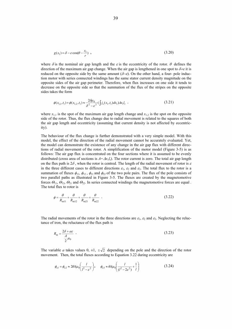
39

)cos()( 11 r

xxg −−= θεδ , (3.20)

where δ is the nominal air gap length and the ε is the eccentricity of the rotor. θ defines the direction of the maximum air gap change. When the air gap is lengthened in one spot to δ+ε it is reduced on the opposite side by the same amount (δ−ε). On the other hand, a four- pole induc-tion motor with series connected windings has the same stator current density magnitude on the opposite sides of the air gap perimeter. Therefore, when flux increases on one side it tends to decrease on the opposite side so that the summation of the flux of the stripes on the opposite sides takes the form

r1111s220

12,111,1 )),((2),(),( lxdxtxjtxtx ∆εδ

δµφφ ∫−

≈+ . (3.21)

where x1,1 is the spot of the maximum air gap length change and x1,2 is the spot on the opposite side of the rotor. Thus, the flux change due to radial movement is related to the squares of both the air gap length and eccentricity (assuming that current density is not affected by eccentric-ity).

The behaviour of the flux change is further demonstrated with a very simple model. With this model, the effect of the direction of the radial movement cannot be accurately evaluated. Yet, the model can demonstrate the existence of any change in the air gap flux with different direc-tions of radial movement of the rotor. A simplification of the motor model (Figure 3-5) is as follows: The air gap flux is concentrated on the four sections where it is assumed to be evenly distributed (cross area of sections is A=∆x1lr). The rotor current is zero. The total air gap length on the flux path is 2δ , when the rotor is centred. The length of the radial movement of rotor is ε in the three different cases to different directions ε1, ε2 and ε3. The total flux to the rotor is a summation of fluxes φ11, φ12 , φ21 and φ22 of the two pole pairs. The flux of the pole consists of two parallel paths as illustrated in Figure 3-5. The fluxes are created by the magnetomotive forces Θ11, Θ12, Θ21 and Θ22. In series connected windings the magnetomotive forces are equal . The total flux to rotor is

m221m2m121m1 RRRRθθθθφ +++= . (3.22)

The radial movements of the rotor in the three directions are ε1, ε2 and ε3. Neglecting the reluc-tance of iron, the reluctance of the flux path is

0

m

2

2

µ

εδA

aR += . (3.23)

The variable a takes values 0, ±1, 2± depending on the pole and the direction of the rotor movement. Then, the total fluxes according to Equation 3.22 during eccentricity are

−≈= 2202ε1ε 2

εµθφφ

llA ,

+

−≈

lllA 1

)2( 2203ε εµθφ (3.24)

40

The change of the absolute value of the total flux over the air gap was calculated with integra-tion over air gap circumference using Equation 3.19 and with Equations 3.24 for the eccentricities of 10% and 25 %. The total flux change percentages were 0.5 % and 3.3 %. The results remained approximately the same for both the sinusoidal model (Eq. 3.19) and the sim-plified model. According to Equation 3.19 the direction of the eccentricity has only about 5 % effect on the change in the total flux over the air gap (about 7 % according to Equations 3.24). If more poles were introduced in the simplified model, the effect of the direction of the eccen-tricity would be smaller than that given by Equations 3.24. The following conclusions can be drawn from the results: 1) The air gap flux tends to change due to the radial movement of the rotor causing a change in the stator EMF and respectively a change in the stator current, 2) the ratio of the magnitude of the radial movement and the air gap length affects the strength of this phenomenon, and 3) the direction of the movement only slightly affects the strength in the change of the air gap flux.

W1

W2

V2

U1

V1

U2

W2

V1

U2

U1

V2

φ12

φ11

φ21

φ22

ε2

ε1

ε3

φ1

φ2

Fig. 3-5 Flux distribution of a four pole induction motor calculated with FEM and a simplified schematic presentation of the main flux paths at synchronous speed.

If the windings producing the fluxes are connected in parallel the results are quite different from the previous ones. The EMF equals over two parallel windings

dt

iLddt

iLde )()( 2211 == (3.25)

where inductances of the windings are L1 and L2 and the currents, respectively i1 and i2. Due to the radial movement of the rotor, the inductance of the winding of one pole decreases whereas the inductance of the other pole increases. Therefore, the current of the first winding increases and the current of the other winding decreases. The total stator current does not change or the change is weaker than in the case of a motor with series connected windings. Furthermore, the parallel windings reduce the unbalanced magnetic pull (UMP) caused by eccentricity according to e.g. Ellison (1997).

41

Unbalanced magnetic pull

When the permeability of the iron is expected to be infinite, the radial stress distribution be-tween the stator and the rotor can be expressed by the Maxwell’s stress equation

0

21

1 2),(),(

µσ txbtx = (3.26)

where µ0 is the permeability of the air and b(x1,t) is the flux density along the air gap. The stress is always attractive as can be read from the equation. This magnetic force is a source of vibra-tion even if the resultant force is zero. When the force distribution is non- uniform, it tries to deform the stator frame, which can be measured as vibration or noise (magnetic noise). The magnetic asymmetries and rotor eccentricity change the force distribution so that the resultant force is unequal to zero. The components of the resultant force can be calculated by the follow-ing equations:

1r1

2

0 0

21

y ),sin(2

),()( dxRltx

txbtF ∫=

π

µ

1r1

2

0 0

21

x ),cos(2

),()( dxRltxtxbtF ∫=π

µ (3.27)

where R is the rotor radius and lr is the length of the rotor. Figure 3-6 illustrates the distribution of the air gap flux and UMP of a balanced two- pole pair motor with dynamic eccentricity (5% of air gap). The flux density is calculated according to Equations 3.17-3.19 (no rotor current).

Several researchers have measured the magnitude of the UMP due to the eccentricity. For ex-ample, Arkkio (1996) measured the 15 kW 4-pole induction motor with 20 % rotor eccentricity. With static eccentricity, the magnitude of the net resultant UMP was 0.39-0.55kN and with the dynamic eccentricity 0.95-1.33kN depending on the load conditions. Equations 3.26-3.27 lead on to greater values than these, because A) the saturation of the iron is not taken into account in the equations and B) there exist parallel loops in the rotor cage. According to Dorrell (1999), these factors may attenuate the real UMP to half of the calculated value.

As a conclusion it should be noticed, firstly, that the air gap flux change is the quadratic func-tion of the degree of eccentricity, and secondly, that the direction of the rotor movement only slightly effects on the magnitude of air gap flux change. On the other hand, the unbalanced magnetic pull is a quadratic function of the air gap flux and affects the magnitude of the bearing impulse and the actual radial movement of the rotor due to the bearing fault. The eccentricity may be mechanically forced (static or dynamic eccentricity) or it can be mechanically free. Then the unbalanced magnetic pull can cause the eccentricity rotating together with the air gap flux.

42

0 50 100 150 200 250 300 350-2

-1.5

-1

-0.5

0

0.5

1

1.5

2

angle round the air gap [°]

B s [T] ,

σ [M

Pa]

σ

Bs

-4000 -2000 0 2000 4000-4000

-3000

-2000

-1000

0

1000

2000

3000

4000

Fy [N

]

Fx [N]

Ω rt

F

Fig. 3-6. Curve shapes of the air-gap flux and stress to the rotor according to the Equations 3.17 and 3.26

in the left figure and net UMP (according equation 3.27) as a function of time in right the figure. Dynamic eccentricity is 5% of the air gap length.

FEM calculus of the air gap flux change due to the rotor eccentricity. Discontinuities of the air gap are often analysed by using the Fourier series. Analysis using the Fourier series is not very practicable if non-stationary changes of the air gap are analysed. Therefore it is very difficult to model the influence of the non-stationary rotor eccentricity analytically, if the effects of the structures of the stator and rotor teeth and saturation are included in the model. It is difficult to model the sudden changes in the air gap length even with the FEM calculus. On the other hand, the non-linear two-dimensional field problem can be solved by FEM calculation in cases of an eccentric and centred air gap. Two FEM models of a 15 kW four-pole induction motor were created, one with a rotor eccentricity of 0% and the other with an eccentricity of 20%. Radial and tangential components of the air gap flux are presented in Figures 3.7 and 3.8. In Figure 3.7 the space vector of stator current is in parallel with the eccentricity and in Figure 3.8 the space vector of the stator current is perpendicular to the maximum spot of the eccentricity.

Changes in the air gap flux are small, but can be distinguished. The described flux distributions are stationary cases. A transition between the central and the eccentric position of the rotor is not illustrated. On the other hand, if during transition a change in distribution takes place, it should induce voltage to the stator winding. In Figure 3-9, a detail of the air gap distribution is illustrated. The change in distribution due to rotor eccentricity is relatively small and the change is influenced by the location of the stator and rotor teeth. Thereby, it is not clear if the change of electromotive force of stator windings can be measured from the stator current.

43

0 50 100 150 200 250-2.5

-2

-1.5

-1

-0.5

0

0.5

1

1.5

2

2.5

Distance [mm]

Flux

Den

sity

[T]

radial

tangential

0 50 100 150 200 250-2.5

-2

-1.5

-1

-0.5

0

0.5

1

1.5

2

2.5

Distance [mm]

Flux

Den

sity

[T]

radial

tangential

Fig. 3-7. Air gap flux density with a rotor eccentricity of 0 % (left) and of 20 % (right). The maximum spot of the eccentricity is parallel with the stator current space vector.

0 50 100 150 200 250-2.5

-2

-1.5

-1

-0.5

0

0.5

1

1.5

2

2.5

Distance [mm]

Flux

Den

sity

[T]

radial

tangential

0 50 100 150 200 250-2.5

-2

-1.5

-1

-0.5

0

0.5

1

1.5

2

2.5

Distance [mm]

Flux

Den

sity

[T]

radial

tangential

Fig. 3-8.. Air gap flux density with a rotor eccentricity of 0 % (left) and of 20 % (right). The maximum spot of the eccentricity is perpendicular to the stator current space vector.

0 5 10 15 20 25 30 35 40 45 500

0.5

1

1.5

2

Flux

den

sity

[T]

Distance [mm]

ecc. 0% ecc. 20%

Fig. 3-9. Detail of the air gap flux distribution of Figure 4-7 in the cases of central rotor and eccentric

rotor.

44

3.3 Behaviour of stator current due to bearing fault

The asymmetrical air gap magnetic field is normally caused by asymmetrical supply voltage or by the rotor eccentricity. The eccentricity changes the air gap permeance and air gap flux. Both dynamic and static eccentricity as well as free eccentricity cause unbalanced magnetic pull (UMP). The UMP tries to increase the eccentricity, in other words, it moves rotor even further from its central position. It has been shown in the paper of Dorrell (1995) that the rotor eccen-tricity can be indicated by stator current analysis.

In practice, some degree of static eccentricity is always present due to manufacturing toler-ances. Therefore, if dynamic eccentricity exists then both types of eccentricities exist (Dorrell, 1997). Then, according to Dorrell, the new rotor fields with frequencies ω±ωr appear inducing EMF’s in the stator winding and producing current components that can be monitored as side-bands of supply frequency in stator current.

When the rotor supporting rolling element bearing has abnormal clearance due to a defect it allows the radial movement of the rotor. If the rotor moves due to a bearing defect it is possible to indicate the bearing defect as in the case of rotor eccentricity. When the ball of the bearing passes a defected spot on a race the clearance between the inner and outer race decreases. The UMP between rotor and stator (or any radial mechanical load) causes the radial movement, which changes the air gap permeance. Therefore the rotating air gap flux modulates the fre-quency of the ball pass frequency.

It was shown in the papers of Schoen (1994a, 1994b) that the characteristic frequency of vibra-tion caused by a bearing defect is modulated to stator current frequency forming new current components at frequencies

...,3,2,1vbib =⋅±= mfmff (3.28)

where f is the frequency of the supply and fvb is the frequency of vibration.

The influence of the radial movement of the rotor can be included in the space vector model of the induction motor originally introduced by Kovács (1959). In the following, the influence of the air gap change is described by varying magnetising inductance as presented in Figure 3-10. Also the leakage inductances change due to the air gap length change but in a summation with magnetising inductance the influence of the change of the leakage inductance can be neglected. The model can explain the relationship between the change of the magnetising inductance and the stator and rotor currents.

urg

RrRs Lσs Lσr

Lm

Ψsg

usg

isg ir

g

j(ωg - ωr )ΨrgjωgΨs

g

Ψrg

+ - - +

Fig. 3-10. The varying magnetising inductance space vector equivalent circuit of an induction motor.

45

The stator and the rotor voltage equations in the arbitrary reference frame g are

gsg

gsg

ssgs j ΨωΨ

++=dt

dR iu , (3.29)

( ) grrg

grg

rrgr ΨωωΨ

−++= jiudt

dR (3.30)

and the stator and rotor flux linkages

grm

gss

gs ii LL +=Ψ , (3.31)

grr

gsm

gr ii LL +=Ψ , (3.32)

where stator inductance Ls is the sum of the stator leakage inductance and magnetising induc-tance Ls=Lσs+Lm and corresponding equation of rotor inductance Lr = Lσr+Lm. In the stator reference frame, the angular frequency ωg is zero.

From Equation 3.29 the following equation is obtained

sss

sss

ss

ss ΨωΨ jiu −−= R

dtd (3.33)

and differentiation of Equation 3.31 in the stator reference frame yields

dtLd

dtLd

dtd )()()( s

rmsss

ss ii

+=Ψ . (3.34)

It is assumed that the supply network determines the stator voltage. The radial movement of the rotor changes the magnetising inductance Lm and thus Ls. If, as a result, the time derivative of the stator flux linkage of Equation 3.33 and 3.34 is changing the stator current must change according to Equation 3.33. On the other hand, if the time derivative of the stator flux linkage does not change then the rotor or stator current must change according to Equation 3.34. In practice, both stator and rotor currents are changing. The division to rotor and stator currents depends on stator and rotor parameters Lσs, Rs, Lσr and Rr .

The amplitude of the stator current transient due to radial movement of the rotor cannot be calculated accurately. However, the value of current transient that cannot be reached can be estimated. The internal radial clearance of the ball bearing allows the radial movement of the rotor. The maximum magnitude of the movement is approximately 10 % of the air gap length of the 15 kW motor. The air gap flux change with 10 % rotor eccentricity was calculated in Chap-ter 3.2. The total (along airgap circumference flux to rotor) air gap flux change percentage was 0.5 %. The time duration of the flux change must be less than the bearing pass interval, which is approximately 10 milliseconds. On the other hand, the magnitude of the UMP with a 10 % rotor eccentricity is less than 10 kN, and the weight of the rotor is not less than 10 kg. Then, accord-ing to Newton’s second law of motion, the rotor movement of 10 % of the air gap length takes more than 10 ms. Therefore the absolute maximum value of the stator current transient is 0.5 % of the stator current according to Equation 3.34 and with the suggestion that the stator induc-tance Ls does not change at all. This value is highly overestimated, but gives a clue that the actual amplitude of the stator current transient is in the class of tens of milliamperes or less. The

46

UMP performs work when it moves the rotor. The energy that is needed to move the rotor to 10 % eccentricity is approximately 0.2 joules and the power consumed is approximately 20 watts.

In addition, the modulating frequency is not the same in all cases. For example, if a significant degree of dynamic eccentricity exists the UMP rotates at rotational frequency modulating also the bearing impulse at this frequency.

3.4 Conclusions

The cyclic bearing faults induce vibration impulses at predictable frequencies. The measured signal, however is a frame response to these impulses and is affected by the magnetic and me-chanical forces that can modulate the impulses according to Equation 3.7. The motor frame is a linear system and the vibration signal should be generated using of the type of 3.7 type of equa-tion in simulations where joint time- frequency analysis is used.

The airgap flux changes due to the radial displacement of the rotor concluding to a stator cur-rent transient. The transient, however, is very small, tens of milliamperes at the maximum.

47

4. METHODS FOR ANALYSIS OF A NON-STATIONARY SIGNAL

Some of the methods that can be used in the analysis of non– stationary signals are described in this chapter. Also, the basic schema of pattern classification is briefly presented. Statistical method for the classification of multivariate data using Mahalanobis distance calculation is explained. A method of finding the critical values of Mahalanobis distances giving appropriate confidence intervals for the classification is presented. The optimisation of the time –frequency window size is introduced.

Frequency spectrum monitoring has become the most usual method in bearing fault detection besides overall level monitoring. In most cases, ordinary Fourier transform is used to obtain frequency information. The main disadvantages of ordinary Fourier transform are that every short duration interference in the signal is spread over the whole frequency band, the frequency components represent the whole time series and that even a slight frequency change in the sig-nal makes it hard to analyse the frequency content. If the frequency resolution is low one cannot separate frequencies that are close together. If, on the other hand, the frequency resolution is increased, the length of the sample is increased and if the signal is time variant, several frequen-cies appear in the spectrum due to time variance. Particularly in the field of diagnosis of rotating machinery the changes in the rotational speed causes smearing of frequency compo-nents. If the rotational speed of the axle is known, the signal is sometimes synchronised to this with a re- sampling procedure.

Recently, the time-frequency analysis has been introduced as a condition monitoring tool in many researches (Forrester, 1989), (Crenna, 1996), (Pan, 1996), (Bonato, 1997), (Paya, 1997), (Staszewski, 1997), (Yazici, 1999), (Yen, 2000), (Kyusung, 2002). An advantage of time-frequency distributions is that they can reveal details of non-stationary signals, signals that evolve with time. In general, time-frequency analysis requires a lot of calculation power and the interpretation of the results require a lot of effort.

Interpretation of the results can be deterministic or stochastic. If it is deterministic, it can be based on heuristic rules or it can be model based, for example. In this chapter, the pattern rec-ognition approach and terms are used. Even if decisions are based on simple rules such as the exceed of limit value of the variable, pattern recognition terminology can be used since the pattern can be visual, temporal or logical (Duda, 2000).

The pattern recognition system consists of sensing, pre-processing, feature extraction, classifi-cation and post processing finally concluding to the decision. The recognition system is illustrated in Figure 4-1. Pre-processing of data includes e.g. the filtering, domain transforms or segmentation of data. Segmentation of data is done, for example, in order to isolate one period of signal or different operation modes from each other. The feature extraction converts the pre-processed data to sets of numerical values namely feature vectors that describe the different classes. The features should be selected so that for patterns of one class (such as healthy bear-ing), the sets of values are as similar as possible and that the sets differs as much as possible from the sets of other classes (such as outer race faulted bearing). In the classification phase, the feature vectors are placed in one or several classes using e.g. template matching, distance calcu-lations or neural networks. The two usual metrics used in statistical pattern recognition are presented in chapter 4.1.2. In the post-processing phase, the output of the classifier is converted into recommendations or estimates or the risk of misclassification is evaluated.

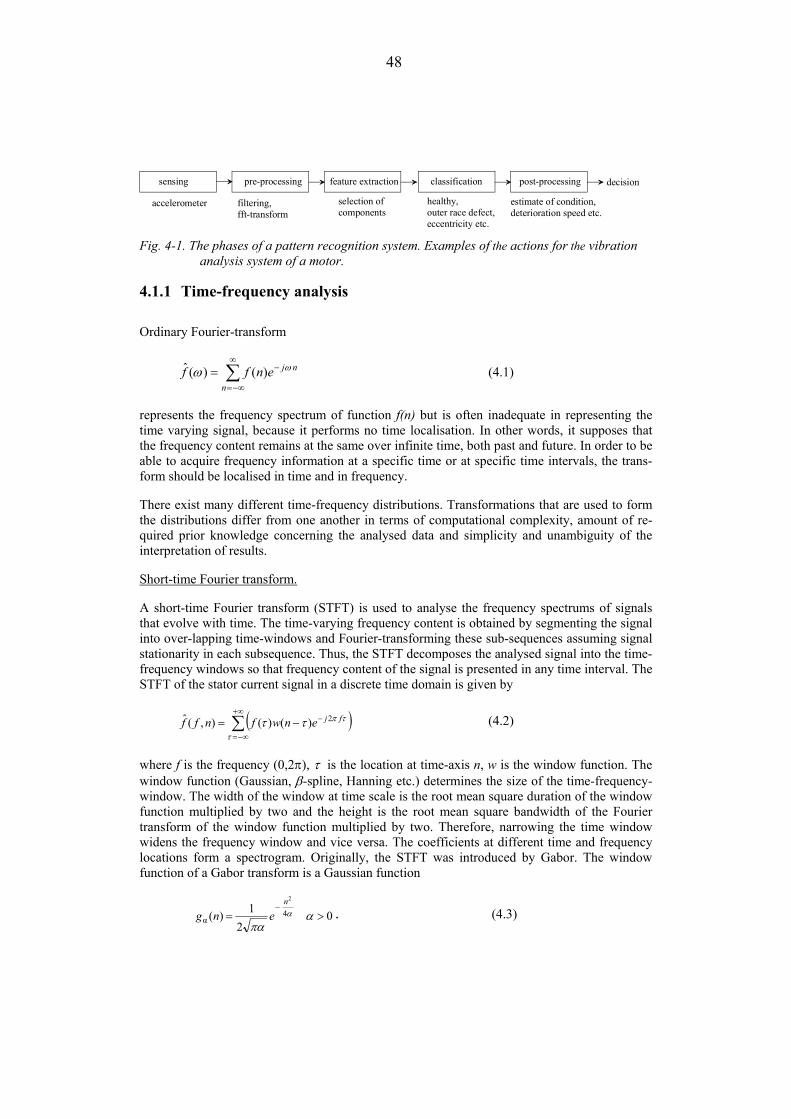
48

sensing pre-processing feature extraction classification post-processing decision

accelerometer filtering,fft-transform

selection ofcomponents

healthy, outer race defect,eccentricity etc.

estimate of condition, deterioration speed etc.

Fig. 4-1. The phases of a pattern recognition system. Examples of the actions for the vibration

analysis system of a motor.

4.1.1 Time-frequency analysis

Ordinary Fourier-transform

∑∞

−∞=

−=n

njenff ωω )()(ˆ (4.1)

represents the frequency spectrum of function f(n) but is often inadequate in representing the time varying signal, because it performs no time localisation. In other words, it supposes that the frequency content remains at the same over infinite time, both past and future. In order to be able to acquire frequency information at a specific time or at specific time intervals, the trans-form should be localised in time and in frequency.

There exist many different time-frequency distributions. Transformations that are used to form the distributions differ from one another in terms of computational complexity, amount of re-quired prior knowledge concerning the analysed data and simplicity and unambiguity of the interpretation of results.

Short-time Fourier transform.

A short-time Fourier transform (STFT) is used to analyse the frequency spectrums of signals that evolve with time. The time-varying frequency content is obtained by segmenting the signal into over-lapping time-windows and Fourier-transforming these sub-sequences assuming signal stationarity in each subsequence. Thus, the STFT decomposes the analysed signal into the time-frequency windows so that frequency content of the signal is presented in any time interval. The STFT of the stator current signal in a discrete time domain is given by

( )∑+∞

−∞=

−−=τ

τπττ fjenwfnff 2)()(),(ˆ (4.2)

where f is the frequency (0,2π), τ is the location at time-axis n, w is the window function. The window function (Gaussian, β-spline, Hanning etc.) determines the size of the time-frequency-window. The width of the window at time scale is the root mean square duration of the window function multiplied by two and the height is the root mean square bandwidth of the Fourier transform of the window function multiplied by two. Therefore, narrowing the time window widens the frequency window and vice versa. The coefficients at different time and frequency locations form a spectrogram. Originally, the STFT was introduced by Gabor. The window function of a Gabor transform is a Gaussian function

02

1)( 4α

2

>=−

απα

αn

eng . (4.3)

49

The Fourier transform of the Gaussian function is also a Gaussian function. Both functions localise to zero. It has been proved that the Gaussian function is the ‘optimal’ window function providing the smallest possible time-frequency window (size of the window= width x height = 0.5). The window size is controlled by variable α.

Bilinear transforms.

Another class of time-frequency distributions is so called bilinear transforms. Unlike spectro-grams, they do not segment the data. Wigner–Ville distribution (WVD) is the basic transform of bilinear transforms. The WVD is based on the instantaneous frequency, which is the derivative of the phase of the signal. For this reason, WVD is made for the complex signals only. The WVD is written

τττ π detstsftWVD tfja

2*a )

2()

2(),( −

+∞

∞−∫ +−= (4.4)

where sa is a signal and sa* is its complex conjugate. An analytic signal sa is formed from a real valued signal s

)(ˆ)()(a tsjtsts += (4.5)

where s is the Hilbert transform

ττ

τπ

dt

sts ∫+∞

∞−−

=1)(1)(ˆ . (4.6)

Bilinear transforms and STFT are used in similar applications and the selection between these transforms is often done experimentally. Further, the success of analysis depends on proper tuning of the parameters.

The Wigner –Ville distribution is widely utilised in a wide area of fault detection of mechanical structures, such as gear transmission or machine tool wear (Forrester, 1989), (Pan, 1996), (Bon-ato, 1997). The WVD can reveal periodic amplitude modulated signals that are not found in spectrograms (Cohen, 1995) because the frequency components or time domain transients are too close together. On the other hand, the bilinear nature of the WVD leads to interference be-tween components in the time-frequency domain. In addition, the cross terms between noise and signal makes WVD noisy. WVD even places the noise at times where the signal is pure from noise. The unambiguity is poor also because of the fact that WVD gives also negative values unlike the spectrogram. The Wigner-Ville distribution is often smoothed by functions with filtering properties (kernels) in order to reduce the interference (i.e. Smoothed Pseudo-WVD). The filtering, however, can also prevent the appearance of weak signal components.

The STFT is the most usual time-frequency distribution because of its good computational efficiency compared to bilinear transformations and because of unambiguous results. The STFT has been largely used in analyses of different properties of mechanical structures and especially for condition monitoring purposes; for example (Crenna, 1996), (Karasaridis, 1997), (Salles, 2000). In condition monitoring of bearings the recurrence of resonance vibration or the modu-lated frequency components of the current signals are analysed. If the window size of the STFT is properly selected it can reveal required characteristics of the signal. In addition, several STFT:s can use various window sizes that can separately reveal details of the signal. The good time-frequency resolution of the Wigner-Ville distribution cannot be fully utilised with multi-

50

component stator current or a vibration signal because interference occurs between every fre-quency component. If, in order to reduce interference, kernel methods are used the adjustment of the parameters prevents straightforward implementation, at least in automatic condition analysis. In Figure 4-2 time-frequency distribution using a Choi-Williams kernel and STFT –distribution of frame acceleration of a motor with a small outer race defect is presented. Choi-Williams distribution can reveal narrow bands in time and frequency domains simultaneously. The STFT was calculated with a window that can present relatively narrow bands in time do-main resulting in very wide frequency bands.

Choi-Williams distribution

t [ms]

f [k

Hz]

0 20 40 60 80 1000

0.5

1

1.5

2

2.5

3

3.5

4

t [ms]

f [k

Hz]

STFT distribution

0 20 40 60 80 1000

0.5

1

1.5

2

2.5

3

3.5

4

Fig. 4-2. Bilinear Wigner-Ville based distribution with a Choi-Williams kernel and STFT distribution of

the acceleration measurement of the motor with a broken bearing. Direct observation of either of the distributions can reveal the bearing pass frequency of 89.7 Hz (Repetition period of verti-cal stripes is 11.15 ms).

Wavelets.

Wavelet transformations have been widely introduced in condition monitoring recently. Wave-lets can divide the signal into time-scale space so that the size of the window at time and frequency (scale) is not rigid (Daubechies, 1990). This is needed especially if information is needed from the wide frequency range.

The motor bearing detection via wavelet analysis using starting current measurement was inves-tigated in the paper of Eren (2001). The starting current was divided into frequency bands using discrete wavelet transform. A three phase, 1 hp, four pole induction motor was tested in the cases of the outer race defected bearing and healthy bearing. According to this reference, the changes between two cases at three frequency bands from 120 Hz to 4 kHz can be found. A weakness in the method is that the small changes in frequency content (scale content) can be recognised only if a comparison between a healthy and broken case can be made under exactly the same conditions. At the motor start up the amplitude of magnetising current is approxi-mately as great as in steady state and the rotational speed is lower (from zero to steady state rotational speed). Therefore, when a bearing ball passes the defected spot of a race the rotor has more time to take its eccentric position. This may result in changes in the permeance and in the air gap flux that are greater than under steady state conditions. Kyusung (2002) has used neuro-predictors and Wavelets for fault detection. In his research, however, the predictors use rota-tional speed and phase voltages in addition to phase currents as inputs. The output of the predictor is a vector of three phase currents. These currents are compared with the measured ones. According to the reference, the classification error (even without knowledge of the bear-ing geometry) is very low.

51

The vibration signal can be analysed without time-frequency distributions. However, these distributions offer one possible way for the feature extraction if automatic classification of fault is required. The calculation effort can be reduced if only some of the resonance band frequen-cies are calculated with STFT with low resolution discrete Fourier-transform. On the other hand, if human based analysis is done, time-frequency distributions can give valuable visual information to the analyser. If time-frequency distributions are used in order to produce features for the analysis, classification and post-processing is required. Possible methods include autore-gressive methods, neural networks or statistical methods.

The stator current signal can change only slightly due to a bearing fault. The signal is time vari-ant even without faults and the radial movement of the rotor due to a fault can be attenuated or amplified due to the resultant of various radial loading forces exerted to the rotor. For this rea-son, the time-frequency representations can reveal changes that could be impossible to detect with time analysis or frequency analysis only. The tininess in the change of the stator current signal means also that statistical analysis is required for the reliable detection of change. Statis-tical analysis is required both for the detection of the change and in order to determine the significance of the change so that the reliability of the classification can be evaluated.

4.1.2 Statistical signal classification using Mahalanobis distance

As mentioned before in this chapter, statistical distance calculations can be used in classifica-tion of signals. In the following, the properties of the most common metrics: Euclidean and Mahalanobis are presented.

Suppose that the frequency spectrum of the stator current includes components that are depend-ent on a bearing fault but cannot be revealed by visual inspection. On the other hand, if the amplitudes of frequency components to be compared are changing under normal operation of the motor, they cannot be compared directly with statistical variables such as mean and standard deviation.

Data can be transformed into a form that is scale and translation invariant (z-score normalisa-tion). The resulting data is called standardised distance and it has a unity standard deviation.

δµ−

=)()( nxnr , (4.7)

where x(n) is the original signal, µ its mean and σ its standard deviation. Values obtained from various measurements are comparable so that the statistical properties such as the mean value and the maximum value describe the shape of the original signal, not the dimensions. The stan-dardised distance can be used in examinations of one feature. If more features are to be considered and the features are statistically independent, the distance of the feature vector x from the class of other feature vectors can be calculated with Euclidean distance or its variant that is made scale invariant using standardised distance:

2

j,d

j,dd2

j,2

j,222

j,1

j,112j ...),(

δδδmxmxmx

mr−

++−

+−

=x , (4.8)

where xi is the value of feature i. mi,j is the mean of the feature i for class j and σi,j is the standard deviation of feature i for class j and d is the number of features. Distance r can be then used for classification. Under each known condition the class mean and standard deviation are calcu-

52

lated. A sample can then be classified by calculation of the minimum Euclidean distance classi-fier, where the distances between the sample and all other classes are calculated and the sample is located in a class of minimum distance.

When features have a tendency to vary together (as is often the case with spectral components), the variance is replaced by the covariance between features i and k:

( )( )∑=

−−−

=n

lll mxmx

nc

1kk,ii,ik 1

1 , (4.9)

where n is the number of samples. The covariances between all features can be written in matrix form

=

)d,d(...)2,d()1,d(.........

)d,2(...)2,2()1,2()d,1(...)2,1()1,1(

C

ccc

cccccc

, (4.10)

The equation of standardised distance can be written in matrix form using covariance

( ) ( )x1

xx2 mxC'mx −−= −r , (4.11)

where r is the Mahalanobis distance between feature vector x and mean vector mx (Mahalano-bis, 1936)

Using the Mahalanobis distance, a comparison between the healthy bearing and broken bearing cases can be done using two basic analyses: detection of a single multivariate outlier and dis-crimination analysis between two populations. In addition to that, if populations differ one can determine if a sample belongs to either population.

In order to determine the difference between two sets of samples, the Mahalanobis distance with common covariance matrix is calculated

( ) ( )yx1

xyyx2 mm'mm −−= −Cr , (4.12)

where r is the Mahalanobis distance between sets x and y. mx and my are the mean vectors and Cxy is the common covariance of the sets. In order to evaluate if the classification is meaningful (hypothesis testing) the confidence interval of Mahalanobis distance is calculated.

The classification of samples is reasonable only if observed differences between sets of samples are real. Also, if the differences are real, does it mean that the same decision rules apply also for the future samples. There are several measures for determination of the statistical significance of distance between the two sets of samples (populations) and their Mahalanobis distances. The critical values for the confidence intervals are not only dependent on the type of problem but also on the sample size, number of features and on the degree of non-normality of the distribu-tion (Mardia, 1971), (Penny, 1996).

53

The optimal error rate OER (Lachenbruch, 1975) is the probability of misclassification:

)2/( rΦOER −= , (4.13)

where Φ is the cumulative normal distribution and r is calculated according to Equation 4.12. A common area of two probability densities, the overlapping coefficient (OVL) that is used as a measure of the agreement between the two sets of samples is

)2/(2 rΦOVL −= . (4.14)

It has been shown (Lachenbruch, 1975) that the Mahalanobis distance with a common covari-ance matrix is F-distributed

)(~)2)(1()1(

12 λ−−+−++

−−+dnd,mFr

mnndmnnm (4.15)

where λ is the noncentrality parameter of F-distribution with a value of

)( nmnm+

=λ . (4.16)

Since the confidence interval for the F-distribution can be calculated also the confidence inter-vals for OER and OVL follow directly. However, the nature of the condition monitoring task (in practical application) is such that it is easier to compare the difference between a single measurement sample and a pre-calculated expectation value of a healthy case. Using this ap-proach, a new covariance matrix is not needed for every new sample. This leads to the calculation of the confidence interval of the single multivariate outlier.

For the detection of single outliers in multivariate data the critical values that provide certain significance levels have to be calculated. The calculation of these critical values is given origi-nally by Wilks (1963). Penny (1996) has given appropriate critical values that can be used for the jacknified Mahalanobis distance calculation. The jacknified Mahalanobis distance calcula-tion means that the covariance matrix and the mean vector of the Equation 4.11 are calculated excluding the feature vector(s) that is tested to belong or not to the group. Based on the results of Krzanowski (1979), Penny has showed that the jacknified Mahalanobis distance is F-distributed

dd,nFdnn

nndr −−−−−

)1)(1()2(~2 . (4.17)

The jacknified Mahalanobids distance calculation has two advantages in practical condition monitoring applications. As mentioned before, the classification would be based on discrimina-tion of a single multivariate outlier. If the covariance matrix is pre-calculated the calculation of Mahalanobis distance is much lighter than in the case of the common covariance matrix. Fur-thermore, using jacknified Mahalanobis distance calculation, the mean vector mx and covariance Cx of Equation 4.11 are not affected by the vectors under test.

Properties and limitations of the Euclidean and Mahlanobis metrics. Fig. 4-3 illustrates the difference between the Euclidean distance and the Mahalanobis distance using the well known four dimensional Fisher’s Iris data. In the figure, only two features are plotted against each

54

other. Contours of constant Euclidean distance are spheres and contours of constant Mahalano-bis distance are ellipsoids. Notice, that the samples of the Iris species marked with dots can be classified well using either metrics but many of the samples representing species marked with stars and plusses can be classified only with a Mahalanobis distance classifier. Euclidean dis-tance classifier does not take into account the shape of the distribution of samples, only the distance from the mean vector. If there are distinct subclasses, for example if samples marked with a plus sign and dots were of the same species, neither of the metrics could classify the data properly. In these cases one should cluster the data and handle subclasses as separate classes. The same problem arises when there exists disturbances in the signal. The disturbed sample can locate far from the majority of samples, changing the location of the mean vector and, in the case of the Mahalanobis metrics, the direction and shape of the distribution. Especially, for condition monitoring purposes when the search for single outliers is used, the disturbances are problem both in training phase and in the post processing phase. If a few samples that differ significantly from others are included in the training data, the properties of the distribution change so that small differences cannot be detected in the post processing phase. On the other hand, if they are not included, the risk of misclassification is obvious in the post processing phase.

Fig. 4-3. Sepal width against petal width of the Fisher’s Iris data containing three species of Iris flower.

Contours of constant Euclidean distance are circles and contours of constant Mahalanobis dis-tance are ellipses.

4.1.3 Method of Yazici

Yazici (Yazici, 1999) has presented the method, in which, the STFT coefficients on selected frequency bands are used to form the feature vectors. A feature vector is a set of STFT coeffi-cients at one time-instant.

),(ˆ),...,,(ˆ),,(ˆ)( L10 nfinfinfin =F (4.18)

where i is the coefficient of STFT obtained from stator current at centre frequency f. L is the total number of features (frequency bands). The Mahalanobis distances between feature vectors of supervision data from a healthy machine are calculated, and the mean value of the distances

55

is used to form the expectation value of the healthy case. When the distance of the test feature vector differs enough from the expectation value, it is concluded to be from the broken case.

4.1.4 Optimal Gabor filter parameter selection for classification

A visual inspection of the frequency spectra of two signals often does not reveal if the fre-quency contents of the two signals differ. Statistical means such as the Mahalanobis distance calculation are used to classify signals or spectra as presented in Chapter 4.1.2. For the proper classification of the transient signals, the selection of time- frequency window size is often critical. If the spectra of two different classes are taken from measurements where only the subject of classification differs the discrimination between classes can be made if adequate difference on some frequency band is found. The difference between two spectra can be found using a method that optimises the Gabor filter so that maximum energy difference of two spec-tra is found. The method is described in detail in the paper “Signal Discrimination Based on Power Spectrum of Filter Response” (Kämäräinen, 2002). The method was originally designed for this project. The method can test the following (Lindh, 2003):

• Evaluate the frequencies that best separate between classes. • Evaluate the size of the time-frequency window that best separates between classes. • Evaluate if the predicted frequency components differ between classes

The method uses normalised representation of the Gabor filter that is written in the time domain

)2(0 0

22

0

)( tfjt

f

eeftg πγ

γπ

−

= (4.19)

and in the frequency domain

( )20

2

0)(fu

feuG−

−

=

πγ

(4.20)

where f0 is the centre frequency and γ determines the duration and bandwidth of the filter.

A. First-Order Statistics

The discrimination between signals is made by discriminative energy functions Ex. The set of optimum filter parameters W is obtained when the difference between energy functions of healthy and broken cases maximised.

0,

maxargˆf

xEWγ

= (4.21)

The first-order optimisation searches the filter parameters that produce a maximum energy difference. The energy difference between a healthy and broken case can be written

2

1

0

2b

1

0

2h )(*)(1)(*)(1

21

−= ∑ ∫∑ ∫

−

=

∞

∞−

−

=

∞

∞−

a

k

a

kdttxtg

adttxtg

aE (4.22)

where xh and xb are the continuous signals for a healthy and broken case and a is the number of samples of any number of data points.

56

Parseval’s relation states

∫∫∞

∞−

∞

∞−

= duuXugdttxtg 22 )()(ˆ)(*)( , (4.23)

where X is the Fourier transform of x. Equation 4.22 can be written in the form

2

1

0

2b

1

0

2h )()(1)()(1

21

−= ∑ ∫∑ ∫

−

=

∞

∞−

−

=

∞

∞−

a

k

a

kduuXuG

aduuXuG

aE (4.24)

and because G(u) is always a positive real

−= ∑ ∫∑ ∫

−

=

∞

∞−

−

=

∞

∞−

1

0

*bb

21

0

*hh

2 )()()(1)()()(121 a

k

a

kduuXuXuG

aduuXuXuG

aE (4.25)

In a discrete form

∑∑∑∑−

=

−

=−=

1

0

*bb

21

0

*hh

2 )()()(1)()()(1 a

k u

a

k uuXuXuG

auXuXuG

aA (4.26)

when

2

21 AE = . (4.27)

B. Second-Order Statistics

Second-order Statistics not only search differences in the power spectra but also search differ-ences in the change of power spectrum bands. For this, the estimates of variances are needed.

= ∫∞

∞−

dttxtgVar2

hi

2h )(*)(δ (4.28)

and

= ∫∞

∞−

dttxtgVar2

bi

2b )(*)(δ . (4.29)

It is supposed that data is normally distributed, then

( )

2h

2h

22

h

h2

1)( δ

µ

πδφ

−−

=

x

ex (4.30)

and

57

( )

2b

2b

22

bb

2

1)( δ

µ

πδφ

−−

=

x

ex (4.31)

For the Gaussian distributions, Fisher’s discriminant ratio (FDR) can be calculated

( )2

h2

b

2hb

hb ))(),((δδµµφφ

+

−=xxFDR (4.32)

in order to measure the distance between distributions. For other cases, the distribution must be estimated.

This can be done with the relative entrophy (Kullback-Liebler difference) (Cover, 1991)

dxxxxxxKL)()(log)())(),((

b

hhbh φ

φφφφ ∫∞

∞−

= (4.33)

or its symmetric version

))(),(())(),(())(),((2 hbbhbh xxKLxxKLxxKL φφφφφφ += . (4.34)

Above measures give discrimination energy functions

2bh2 )))(),((2(

21 xxKLE φφ= (4.35)

and

( )2

2h

2b

2hb

3 21

+

−=

δδµµE . (4.36)

Energies are optimised according to Equation 4.21 using the gradient method. A detailed description of the method is presented in reference (Kämäräinen, 2002).

4.2 Conclusions

The vibration signal can be analysed in the time domain or in the frequency domain. However, also joint time- frequency analyses can be used as a part of a feature extraction in the case of an automatic classification of signals. Furthermore, the time-frequency representations provide information of the time varying signals for the human made analyses as seen in Figure 4-2. The change in the stator current due to a bearing fault is tiny and time varying. In order to extract these changes time-frequency analysis may be required. Furthermore, statistical pattern recogni-tion may be needed for the classification. According the equation 3.28, some frequency components change due to the bearing fault, others not. Mahalanobis metrics provides means for handling the covariance between frequency components. Therefore, it is selected for the classification between healthy and broken cases.

58

5. TESTING EQUIPMENT

A testing equipment was constructed in order to test bearing fault indications of an induction motor. In this chapter, the general description of equipment is given and the characteristics of the measurement devices are described.

Motor

A 15 kW four-pole induction motor ABB M2 AA 160 L4 was used. The rated current is IN= 28.5 A when delta-connected to 400 V grid. The Motor was loaded with an converter driven DC-motor. The DC-motor and the motor under test were connected together with a toothed belt and with a bearing supported axle with a band coupling. The reduced moment of inertia of the DC-motor on the induction motor axle is approximately J=0.15kgm2. Testing equipment is illustrated in Fig. 5-1.

Fig. 5-1. A view of the testing equipment.

Bearings

The bearings of the induction motor are single row deep groove ball bearings, type 6209. Bear-ings have 9 balls or 10 balls. Measurements were taken with seven bearings: two healthy and five with radial holes in the outer race (Fig. 5-2: hole diameters 2 mm and 5 mm). The meas-ured radial clearances between the inner and outer race of the bearings A to D were less than 20 µm from centre position. The clearances of bearings E to G were between 30 µm and 45 µm. Characteristics of bearings are presented in table 5-1. The internal clearance in the rolling ele-ment bearing has effects on the vibration level and heat-generation and consequently on the noise level and to the fatigue life. The internal radial clearance class of the bearing of the elec-tric motor (CM) is usually tighter than class “normal” in order to reduce noise. However classes ‘normal’ and C3 are used widely in electric motors and in some cases big induction motors are equipped with C4 bearings.

59

Table 5-1. Radial clearances of type 6209 bearings.

Bearing6209 class min [µm] max [µm]

A 0 normal 6 23B 2 normal 6 23C 5 normal 6 23D 0 C3 18 36E 2 C3 18 36F 0 C4 30 51G 2 C4 30 51H 5 C4 30 51

CM 9 17C2 1 11

Hole Φ [mm]

Internal clearance

not testednot tested

Fig. 5-2. 6209 ball bearings with ∅2 mm and ∅5 mm holes drilled through the outer race

The bearing faults presented in chapter 2 were divided into cyclic and non-cyclic faults. The bore in the outer race represents well the cyclic faults of outer race (e.g. fatique, crack). The non-cyclic faults can be indicated with overall vibration level triggering. These non-cyclic faults are not under consideration in this thesis.

Measurements

Stator current was measured from one phase with a current clamp. In addition, radial vibration was measured with a piezoelectric accelerometer and with a micromachined silicon accelerome-ter chip. The measurement configuration is illustrated in Fig. 5-3.

60

M M

DC Drive DC Motor Induction Motor

3 Phase Supply400V 50Hz

Notch Filter

Database

3 Phase Supply 400V 50Hz

Current ProbeVibration Meter

Anti Aliasing Filter

Torque and RPM Meters

Display Unit

Amplifier

AmplifierAnti Aliasing Filter

AD Converter Fig. 5-3. Measurement configuration for bearing damage detection.

Current measurement configuration consists of 1. Fluke AC-current probe 80i-1000s capable to detect transients of 5 mA. 2. Notch filter with stop bands at 50 Hz, 250 Hz and 350 Hz. 3. Analog amplifier that increases SNR and resolution in AD-conversion 4. Fourth order Bessel-type anti-aliasing filter with 3dB attenuation at 400 Hz 5. 16 bit AD-conversion with National Instruments analog IO-card and storing to file

The ability of the current probe to measure small current components was tested with four val-ues and with four different frequencies between 20…200 Hz. The probe could measure a current of less than 5 mA. The iron of the coil in the probe was not saturated under full load conditions.

Table 5-2. The test of the ability to measure small amplitude current signals. The type of the current probe is a Fluke AC-current probe 80i-1000s.

The notch filter was used in order to attenuate the biggest current components at 50 Hz, 250 Hz and 350 Hz. Then the 16- bit AD-conversion could provide enough resolution so that compo-nents smaller than 1 mA could be detected. The frequency response of the notch filter is illustrated in Figure 5-4. The disadvantage of the notch filter is that it greatly attenuate the bear-ing induced components if they are near to the stop bands of the filter.

I RMS [mA] V RMS [mV], f =20 Hz V RMS [mV], f =50 Hz V RMS [mV], f =100 Hz V RMS [mV], f =200 Hz5 0.2 0.4 0.5 0.5

10 0.4 0.7 1 120 0.7 1.3 1.8 250 1.7 3.5 4.4 4.9

61

Fig. 5-4. The measured frequency response of the notch filter used in stator current measurements.

The piezoelectric accelerometer serves as a reference measurement for the determination of bearing pass frequency in parallel with the stator current measurements. The piezoelectric ac-celerometer is also used in parallel with the micromachined accelerometer in the evaluation of the micromachined sensor ADXL105.

A reference vibration measurement consists of a SKF accelerometer CMSS786A, a constant current amplifier and a 4. order anti-aliasing filter with 3 dB attenuation at 8 kHz. The acceler-ometer has a 1 dB amplification at this frequency rising up to 3 dB amplification at 14 kHz. The nominal resonance frequency of the accelerometer is 30 kHz. A signal is AD-converted and stored in the same manner as the current signal.

The measurement configuration of the micromachined accelerometer consists of a signal ampli-fier, a 4. order anti-aliasing filter with a 3 dB attenuation at 3 kHz and AD-conversion as for the other measurements.

62

6. TESTS FOR THE DETECTION OF A BEARING FAULT USING STATOR CURRENT MEASUREMENTS

In this chapter, the verification of the feasibility of the stator current measurement as a bearing fault indicator is experimentally tested. The main tasks are, firstly, to clarify the effects of the outer race bearing defect on the stator current of a 15 kW induction motor. Secondly, the practi-cal importance of the results is estimated from a condition monitoring point of view. The effects of the radial movement of the rotor are first tested with the radial shocks to the motor axle when the motor is magnetised with DC-current. The spectrum of the stator current signal is analysed. Included is a Mahalanobis distance calculation based classification of the stator current signal resulting from analyses of a simulation and experimental results using actual measurements. The optimisation of the time-frequency window is introduced. The optimisation is done in order to find the windowing parameters that maximise the difference between healthy and broken case data. The purpose of this chapter is to test the practicability of the stator current measure-ment based indication of the bearing condition. The tests are done using the measurement setup in Chapter 5.

6.1 Change of air gap in a DC-magnetised induction motor

The stator current signal is time varying even when the motor is running at steady state. Further, the signal has many frequency components due to a non-ideal motor structure and polluted supply voltage. Stator and rotor teeth, magnetic unbalances, the discrete number of slots etc. make it hard to separate the transient signal that is originated from the radial rotor movement from these other components. In addition, modulation effects of the rotational magnetic fields and mechanical radial forces prevent the study of the magnitude and shape of the induced stator current transient when the motor is running.

On the other hand, the stator windings can be magnetised with direct current. The same magni-tude of the magnetising current as in normal operation mode can be fed from the DC-voltage source. The signal contains only one frequency that does not modulate the transients created by the change in magnetic properties of the motor. The magnitude of the current transient as a function of the size of the rotor movement can be found. The information obtained from the test can then be used in the simulation using an artificially created signal as a modulating signal. Hence, the actual effect of the radial movement of the rotor on stator current of the running motor is found excluding the effects of the saturation of the stator and rotor iron.

The influence of the sudden change in the air gap length was tested when the stator windings were magnetised as illustrated in Figure 6-1. The radial movement of the rotor was caused by the magnetic pull in the first test and by effecting the rotor with a pendulum in the second test. The end shield at the D-end of the motor was removed and the rotor was supported with alumin-ium and copper strips. Three thicknesses of supporting strips were used: Strips of 0.5 mm were used to centre the rotor and the strips of 0.3 mm or 0.4 mm were used to stop the radial move-ment of rotor at its eccentric position. In the first test, the radial movement was caused by the magnetic force when one of the thicker strips was pulled off from the air gap.

The results show that equalising circulating currents in the rotor and stator don’t flow so that they prevent the indication of the induction of the stator current due to the rotor movement. A test result is plotted in Figure 6-2. The motor was magnetised with 7A current that is approxi-mately half of the magnetising current of the motor’s normal full load condition. A 40 %

63

change in the air gap length caused a stator current transient of ipp=260 mA. The change in the air gap in a case of the actual bearing fault is much smaller, approximately 1-10 % of the nomi-nal air gap length.

DC-POWER

SERIES COIL L

MOTOR

Fig. 6-1. DC-supply of the induction motor in the DC-magnetisation test.

0.5 0.55 0.6 0.65 0.7 0.75 0.8 0.85 0.9 0.95 1-0.2

-0.15

-0.1

-0.05

0

0.05

0.1

0.15

0.2

time [s]

curre

nt [A

]

Fig. 6-2. Stator current transient due to radial movement of a rotor. Stator was magnetised from a

DC-voltage source. The current clamp does not measure the direct current only the transient. The magnetising current was approximately half of the nominal reactive cur-rent of the motor at full load.

The size in change of the stator current is of course dependent on the impedance of the supply-ing network also. Therefore, the effect of the size of the inductance of the supplying network was analysed. Coils were connected in series with motor as presented in figure 6-1. Stripes of 0.4 mm were used to centre the rotor (20 % free eccentricity) and the radial shock on to rotor was given with a pendulum with a rubber weight.

Table 6-1 presents results for different coil sizes. The first observation is that when the accelera-tion of radial movement is parallel with the air gap flux the induced current can be 5-6 times greater than in the case of perpendicular movement. This result supports the theory that rotating air-gap flux and consequent UMP modulates the stator current transient effectively. As stated in the Chapter 3.2, the direction of the radial movement of the rotor has only slight influence on the change in the stator flux itself, but the UMP may affect both the size and the speed of the movement. Another result is that normal variations in the network reactance cannot prevent the appearance of stator current transient due to radial movement of the rotor. For example, the inductance of a 500 kVA distribution transformer is about 0.05 mH (400 V side) and the induc-

64

tance of a low voltage motor cable per one kilometre has, roughly, the same order of magnitude. In this test, a 65 mH series coil approximately halved the peak value of the current transient.

Table 6-1. Peak to peak values of the stator current transients for different series coil (L) values. The radial rotor movement (acceleration a) is directed perpendicular to (⊥) and parallel with ( ||)

the maximum air gap flux.

L [mH] I [mA] (a ⊥ B ) I [mA] (a || B )0 15.8 91.265 10.2 50.4130 9.2 30.5195 11.5 21.6

The relationship between the degree of radial movement of the rotor and the acceleration level and the stator current transient magnitude was analysed with simultaneous measurements of the size of the radial movement of the rotor, the acceleration level and the amplitude of the stator current. The results are presented in Table 6-2. The ratio between the displacement and accel-eration level differs from actual running motor ratio. Anyhow, the test showed that 10 mA current transient already required a combination of approximately 100 µm displacement and a shock that resulted in frame acceleration level about 2 g:s. Therefore, it is probable that the current transient in the running motor cannot reach values more than tens of milliamperes at the maximum. A minimum shock that can be measured by measurement configuration described in chapter 5 was also tested with the pendulum test. This was done in order to ensure that a meas-urement chain (current clamp, notch filter, AAF-filter, quantisation) doesn’t attenuate the stator current transient caused by the slight radial movement of the rotor. The minimum frame accel-eration that could be measured reliably was less than 0.3 g with a rotor displacement of approximately 10 µm. With the smaller values the signal was covered with the noise of the current clamp and by the DC-voltage source.

Table 6-2. Change in air gap length, frame acceleration and peak to peak value of the stator current transient. Acceleration value is an average value of the positive and negative peak values.

∆σ [µm] a [g] i pp [mA] 370 6.5 109.0360 6.5 105.3352 6.2 97.4310 5.8 76.0269 5.3 53.4212 4.4 22.3139 2.8 11.394 1.8 8.186 1.5 7.689 1.5 7.456 0.8 6.253 0.8 6.012 0.3 5.6

The bearing A (internal radial clearance class ‘normal’) was installed and the motor was assem-bled. The pendulum test with the DC magnetisation was repeated. Maximum shock (energy about E= 3J) produced an approximately 10 µm (peak to peak) change in the air gap length, 12 mA (peak to peak) stator current transient and 8 g peak stator frame acceleration. The wave-forms are presented in Figures 6-3 and 6-4. The supporting bearing allows the rotor to move only slightly, resulting in a very small change in the stator current but a very high acceleration (hundreds times larger than the minimum that can be detected by an acceleration measurement).

65

4 5 6 7 8 9 10-4

-2

0

2

4

6

8

10

t [s]

∆ σ

[ µm

]

4 5 6 7 8 9 10-10

-8

-6

-4

-2

0

2

4

6

t [s]

a [g

]

Fig. 6-3. Change in air gap length (∆σ) and radial acceleration (a) of stator frame when E=3 J

radial shocks are applied to the rotor axle.

4 5 6 7 8 9 10-10

-8

-6

-4

-2

0

2

4

6

8

t [s]

i [m

A]

Fig. 6-4. Stator current transient when radial shocks of energy of 3 joules are applied to the rotor

axle with a rubber coated steel pendulum.

66

Conclusions

Test results clearly show that even a small change in the air gap length induces a measurable stator current transient. Measurements support the theory that a rotating flux and an unbalanced magnetic pull modulate the current transient caused by the radial movement of the rotor. Fur-thermore, the inductance of the supplying network cannot remarkably attenuate the appearance of current transient in stator current. On the other hand, if the radial movement of rotor is small, the stator current change is only a couple of milliamperes. Poor SNR (Signal to Noise Ratio) makes it hard to separate the stator current transient even from DC-current in a standstill motor.

6.2 Methods using frequency spectrum of the stator current

Schoen has shown in his paper (Schoen, 1995) that vibration of the rotor is modulated into stator current. In the case of a motor with the broken bearing, the predictable frequency compo-nents are present in an ordinary Fourier-spectrum of the stator current. In his research, stator current signal spectra were plotted and visually inspected. He concluded that spectrum peaks caused by bearing damage were detectable and sufficiently distinct as an indicator of the dam-age. In this chapter, non-averaged and averaged frequency spectra are formed then visually and statistically analysed. The averaged spectrum can reveal small amplitude components that otherwise could be covered by noise. On the other hand, if the frequency and amplitude of this small amplitude signal component fluctuates, the component can cease due to the averaging process. Statistical methods are needed because it is impossible to visually distinguish time variant small amplitude components from the noise.

Besides the averaging process the non-stationary stator current signal can be analysed by Fou-rier-transforming signals at various time periods and by comparing results with healthy and broken case signals. The indication of a fault is made if the modulated bearing pass frequency components change significantly when compared to other frequency components. The compari-son between components is made statistically in order to be able to deal with the variation in results.

6.2.1 Averaged power spectra of a stator current signal

The testing equipment of Chapter 5 was used for the collection of the current measurements. Two 4096 point Fourier spectra were formed by averaging 40 non-overlapped samples. The sampling frequency was 3 kHz. The averaging of spectrum was used in order to reduce noise. Fig. 6-5 presents the averaged power spectra of healthy and broken bearing cases. No visible difference between healthy and broken cases could be found on modulated frequencies at a measured vibration frequency of 89.7 Hz. According to Equation 3.28, the modulated frequency components should appear at frequencies fib=39.7, 129.4, 139.7, 229.4, 308.8, 319.1, 398.5, 408.8, 488.2, 498.5, 577.9, 588.2, 677.9 Hz. According to the theory, the amplitudes in the spectra at these frequencies should be larger in broken cases than in healthy cases. The biggest difference is visible at 201 Hz, which is not a modulation of the bearing pass frequency. Fur-thermore, the component is larger for the healthy case data.

67

0 100 200 300 400 500 600 700 800-60

-40

-20

0

20

40

60

frequency [Hz]

dB

Power spectrum

Fig. 6-5. Averaged power spectra of stator current of a 15 kW 4- pole induction motor. X-marked

curves are values for a healthy case and red solid lines are values for a broken case (bearing B: φ2 mm hole in outer race). The biggest difference is visible at 201 Hz, which is not a modulation of the bearing pass frequency. Furthermore, the component is larger for the healthy case data than for the broken case data.

Conclusions

Statistical methods are needed because it is impossible to visually distinguish time variant small amplitude components from noise.

6.2.2 Classification of power spectra of stator current signals using Maha-lanobis distance calculation

Classification problem. The classes are healthy bearing (Ch) and outer race damaged bearing (Cb). To discriminate between a healthy and broken cases it is only needed to know if some of the features change significantly between cases. A set of measurements from the healthy case is used as training data. An approximate critical value is calculated using the mean value m(r) and standard deviation δ(r) of the calculated Mahalanobis distances

)()(limit rkrmd δ+= . (6.1)

If the tested sample gives a distance greater than the limit dlimit the sample is classified to class broken Cb. The value k gives a distance from the mean in a unit of standard deviations.

Three sets of measurements were formed from 40 measurements in each set. One set of meas-urements from a healthy case was used as a training set (Shl), another as a test set (Sht). The

68

4096 point Fourier spectra of samples were formed. A frequency range from 0 Hz to 732 Hz was divided into100 sections (subsets s) of ten consecutive spectrum values. This was done in order to reduce the feature space. Thus, one feature of a feature vector represents a frequency range of ∆f= 0.73 Hz. With the test motor, the 0.73 Hz change of the outer race fault induced vibration frequency is caused approximately by the 22 rpm change in rotational speed. In order to achieve reliable results, a rotational speed variation was kept in range the of ±3 rpm during measurement and between measurements used in this calculation.

The feature vectors were formed for subsets s as follows:

)9(ˆ),...,2(ˆ),(ˆ),(ˆ)( sssss ffiffiffifif ∆∆∆ +++=F (6.2)

where î is the power spectrum coefficient, fs is the starting frequency of the subset s. In every subset, the Mahalanobis distance was calculated A) between two sets of feature vectors for the healthy cases (between Shl, Sht) and B) between a set of feature vectors for the healthy cases and for the broken cases (between Shl, Sb).

The mean, the maximum and the standard deviation of the Mahalanobis distances were calcu-lated. The mean values of the Mahalanobis distances of the feature vectors are presented in Fig. 6-6 and the maximum values in Fig. 6-7. There are only two peaks in Fig. 6-6 that correspond with the modulated bearing frequencies. These modulated bearing frequencies are 229,4 Hz and 319,1 Hz (m=2,3 in Equation 3.28).

The subsets that cover the calculated bearing frequencies fib were selected. In order to analyse the significance of the calculated Mahalanobis distances, the distances are related to the vari-ance of healthy case distance of band in question. The value of k in Equation 6.1 is calculated when the mean distance of broken case is placed to a limit distance dlimit. The term k then de-scribes the difference between the broken class Cb Mahalanobis distances and the distribution of the healthy test class Cb Mahalanobis distances.

Table 6-3 represents the values plotted in Fig. 6-6 in the ranges that cover the modulated ball pass frequencies. At 229,4 Hz where the peak is visible in Fig. 6-6 the value k is still too low for the classification because the healthy test case Mahalanobis distance and its variance are also relatively large. Another set of samples of 3x40 files is presented and values of k are calcu-lated in Table 6-4. The maximum value of k is at frequency range containing ball pass frequency of 229,4 Hz. On the basis of these results, it is possible to see that there might be a difference between the frequency spectra in broken and healthy cases. Still the differences are so small that they may be due to normal variation of samples caused by noise, disturbances, small differences in load conditions etc. Furthermore, the Mahalanobis distances between healthy cases are so large that they could be indicated to be from a different distribution also.

69

0 100 200 300 400 500 6000

500

1000

1500

frequency [Hz]

mea

n va

lue

of M

ahal

anob

is d

ista

nces

Fig. 6-6. Mean values of the Mahalanobis distances of frequency components from healthy bearing data of stator currents. Distances of broken bearing data (solid line) and healthy bearing data (dotted line) are presented as a mean value of 40 samples in both cases. Modulated bearing frequencies are marked with the +-signs.

0 100 200 300 400 500 6000

1000

2000

3000

4000

5000

6000

frequency [Hz]

max

. Mah

al. d

ist.

Fig. 6-7 Maximum values of the Mahalanobis distance of frequency components from healthy bearing data of stator currents. Distances of broken bearing data (solid line) and healthy bearing data (dotted line) are presented as a mean value of 40 samples in both cases. Modulated bearing fre-quencies are marked with the +-signs.

70

Table 6-3. Sample mean values and standard deviations of Mahalanobis distances D at frequency bands where modulated frequencies fib of the bearing ball pass frequency 89.1 Hz are situated. k is a measure of the difference between healthy and broken case distances approximately in stan-dard deviations.

f ib[Hz] D healhy D broken σ healthy σ broken k39.7 24.32 19.60 26.13 24.70 -0.18

129.4 22.66 15.24 23.99 12.36 -0.31139.7 14.92 15.08 7.76 10.04 0.02219.1 23.30 15.05 26.77 12.93 -0.31229.4 178.94 507.21 363.66 486.87 0.90308.8 22.64 20.79 20.33 12.10 -0.09319.1 13.72 11.92 9.50 7.98 -0.19398.5 24.32 21.05 16.37 17.59 -0.20408.8 21.10 34.84 14.91 50.63 0.92488.2 13.11 18.58 6.48 9.77 0.85498.5 24.91 69.73 26.33 55.23 1.70577.9 21.61 32.22 11.01 18.76 0.96588.2 21.77 21.21 15.75 12.40 -0.04

Table 6-4. Sample mean values calculated as in Table 6-3. The values are calculated using another set of 40x3 sample files.

f ib [Hz] D healhy D broken σ healthy σ broken k39.7 26.1 15.7 30.9 11.6 -0.3

129.4 16.4 16.5 14.9 22 0.1139.7 15.2 16.1 9 6.6 0.1219.1 21.2 15.6 33.8 18 -0.2229.4 203.1 1094.7 407 271.3 2.2308.8 19.3 18.4 17.2 13.2 -0.1319.1 13.1 15.9 9.4 9 0.3398.5 17.5 25.6 11 16.4 0.7408.8 15.9 32.5 10.6 31.5 1.6488.2 13.1 21.4 6.7 27.4 1.2498.5 28.1 81.6 33.1 55.7 1.6577.9 20.2 25.5 16.6 16.3 0.3588.2 16.9 17.3 12.2 9.4 0

6.2.3 Simulation of STFT and the Mahalanobis distance calculation with a test signal

In order to overcome the difficulties caused by the time-varying stator current signal, short-time Fourier transforms can be formed and statistically analysed. Before the actual measurements are analysed, the performance of the analysis method should be tested. Owing to the stochastic

71

nature of the stator current signal, the performance test of the method is done using artificially created signals with known characteristics.

The simulation is done in order to test the method presented in Chapter 4.1.3 and to test the influence of the four factors on the Mahalanobis distance based classification of bearing faults. These factors are the non-sinusoidal time varying air-gap permeance, time varying unbalanced magnetic pull (UMP), radial rotor vibration caused by other factors than the bearing fault and the noise in the measurement chain.

The DC-magnetisation test of Chapter 6.1 indicated that the magnitude and the direction of the air gap flux influence in the induced stator current. Non-sinusoidal spatial distribution of the air gap permeance causes time variation to the air gap flux in a rotating motor. On the other hand, the air gap flux and the dynamic eccentricity of the rotor influence the magnitude and the direc-tion of the UMP.

The simulation is as follows: The radial movement of the rotor is described with the signal with transients it. This artificially created signal is modulated with an artificially created air gap flux is and consequent UMP. The time variation of the air gap flux, of the UMP and of the radial rotor movement is described as a noise of signals is and it. The resulting signal io is analysed statistically.

The information on the shape and amplitude of the stator current transient obtained from the DC-magnetization test (Chapter 6.1) is used in the simulation. The duration of the transient wave in signal it was limited according to the bearing structure and the rotational speed of the test motor. This leads to transients of a duration of approximately 3 milliseconds. Transients are repeated at the characteristic bearing frequency and modulated to continuous stator current signal (Figure 6-8).

The simulation uses the following procedure and simplifications: 1. The time variance of amplitude of the UMP is described partly by a random variation

in the amplitude of the transients in it and partly by noise. The size of variation is 20 % of the amplitude.

2. The noise is added to the signal it to describe the radial vibration of the rotor caused by other factors than the bearing fault.

3. The modulating air gap flux signal is is the same signal as the stator current signal. This simplification can be done without great influence on the classification results. Noise is added to the signal to describe the effects of time variant non-sinusoidal spa-tial distribution of the air gap flux and time variation of the UMP. UMP is the resultant of the integration magnetic force over the whole air gap and changes due to changes in the air gap flux and the momentary eccentricity of the rotor

4. The noise in the measurement chain has the same effects as the noise in the signal is.

72

0 50 100 150 200 250-40 -30 -20 -10

0 10 20 30 40

is it

Fig. 6-8. The simulation uses two artificially created signals it and is. The stator current transient signal it

(100x amplified in the drawing) is modulated to the stator current (air gap flux) signal is. Both signals have noise added.

Signals and classification

One hundred files including signal io were formed. Half of the files represented healthy cases without transients in the signal it , other files represented broken cases. For the both cases, sig-nals it and is have noise added. The combinations of signal to noise ratios (SNR) are found in Table 6-5.

The classes are healthy bearing (Ch) and outer race damaged bearing (Cb). Three sets of files were used. The first set was used as a healthy case training set (Shl), another as a healthy case test set (Sht) and the third as a broken case test set (Sb).

The STFT transforms of simulated signals io were calculated to form coefficients with the time-frequency windows (size 0.6Hz x 0.7s). Spectrograms of signals are presented in Figures 6-9 and 6-10. Two frequencies were chosen on both sides of the calculated characteristic bearing frequency. Hence, the estimated vibration frequency is allowed to have an error of ±1.2 Hz. The coefficients of STFT at the chosen frequency ranges formed the feature vectors according Equa-tion 4.18. At every test 750 feature vectors in each set were tested.

The significance levels of the differences were estimated using F-distribution as presented in Chapter 4.1.2. The critical values (CR) of the 95% confidence level for single outliers were calculated using Equation 4.18.

Using Equation 4.11, the jacknified Mahalanobis distances were calculated between each fea-ture vector of sets Sht and Sb and vectors of healthy case learning sets Shl. Distances were calculated separately for all combinations of signal to noise ratios in Table 6-5. The mean Ma-halanobis distance between the feature vectors in the set Shl was used to form the expectation value for class Ch. The mean value and the variance of the distances were calculated for all the sets. These values are presented in Table 6-5.

The significance level of the difference between the vector and learning set was estimated by using F-distribution as presented in Chapter 4.1.2. The critical values (CR) of the 95% and 99%

73

confidence levels for single outliers were calculated using Equation 4.18. If the distance of the tested vector exceeds the critical value it is located to broken class Cb. The numbers of outliers in the test set Sht (no stator current transients) and in the broken case set Sb (signals with stator current transients) are shown in Table 6-6.

As a conclusion, it is observed that:

A) Noise does not change the centre of the learning class (the mean value of the Mahalanobis distance of learning class remains the same regardless of the noise, Table 6-5).

B) Noise in the signal it that corresponds to the normal radial vibration of the rotor cannot hide the influence of the radial movement at characteristic frequencies.

C) Noise in the signal is (which describes the combination of the time varying distortion of modulating air gap flux and time varying UMP) can make the indication of the fault impossible. This is illustrated in the 100-bin histogram of Figure 6-11 where the frequencies of distances less than one hundred are plotted in bins from 1 to 99 and the frequency of distances more than 99 in the last bin (notation >100). Comparing the right hand plot of Figure 6-11 and the last lines of Tables 6-5 and 6-6 one can notice that even if the mean distance of the broken case is twice the value of the healthy case the risk of a misclassification is significant. There are only one or a few broken case feature vectors whose Mahalanobis distance differs a lot from a healthy case and the majority of the distances don’t differ at all. If these few cases are used to indicate bearing damage, also the disturbances may lead to misclassification. On the other hand if a few feature vectors that differ a lot from the majority of vectors are neglected, no difference between sets can be found.

The increase in the eccentricity increases the UMP. If the rotor rotates centred the UMP is small and unstable. If due to worn bearings, for example, the rotor has a great degree of eccentricity the UMP increases (great SNR of is ).

Time

Freq

uenc

y

0 0.5 1 1.5 2 2.5 3 3.5 40

50

100

150

200

250

300

350

400

450

500

Time

Freq

uenc

y

0 0.5 1 1.5 2 2.5 3 3.5 40

50

100

150

200

250

300

350

400

450

500

Fig. 6-9. Spectrograms of an artificially created stator current signal from a broken and healthy case. The SNR of transient is 20 dB and the SNR of the modulating signal is 70 dB.

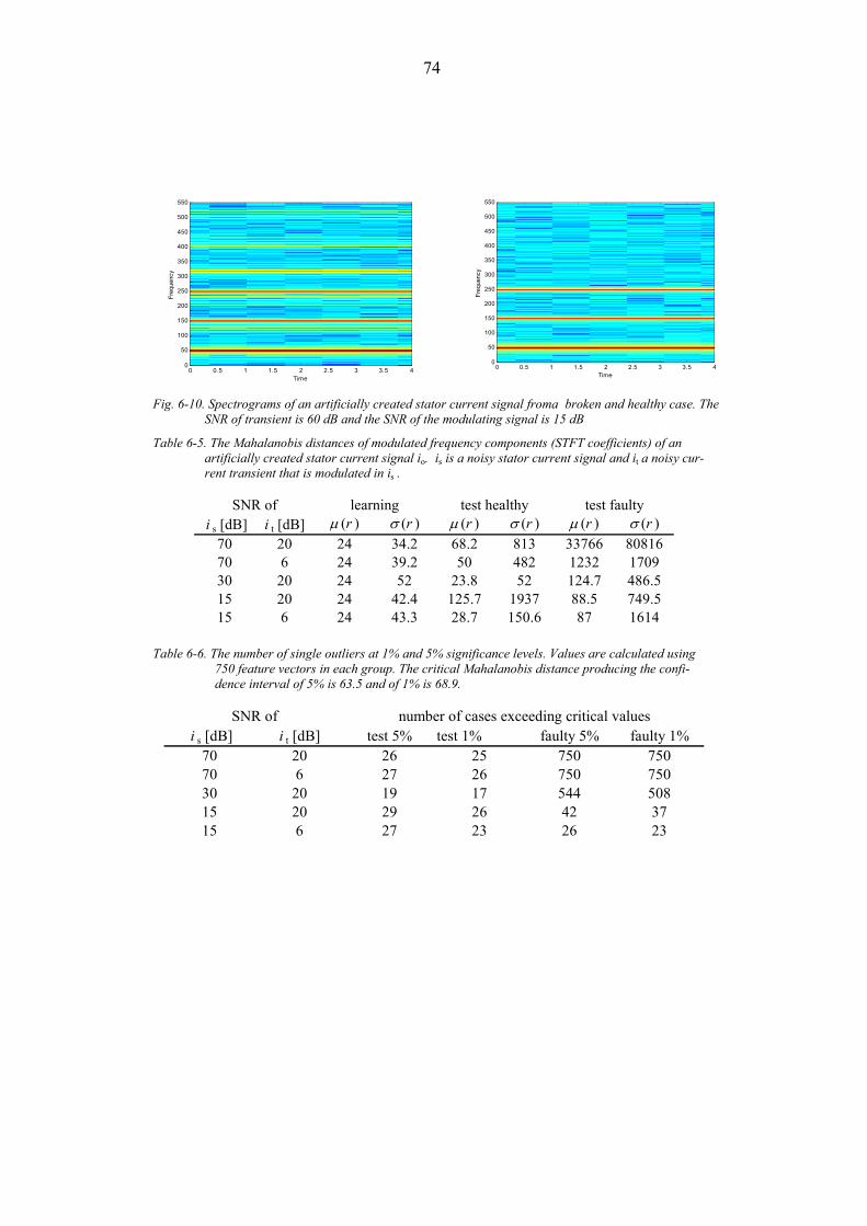
74

Time

Freq

uenc

y

0 0.5 1 1.5 2 2.5 3 3.5 40

50

100

150

200

250

300

350

400

450

500

550

Time

Freq

uenc

y

0 0.5 1 1.5 2 2.5 3 3.5 40

50

100

150

200

250

300

350

400

450

500

550

Fig. 6-10. Spectrograms of an artificially created stator current signal froma broken and healthy case. The SNR of transient is 60 dB and the SNR of the modulating signal is 15 dB

Table 6-5. The Mahalanobis distances of modulated frequency components (STFT coefficients) of an artificially created stator current signal io. is is a noisy stator current signal and it a noisy cur-rent transient that is modulated in is .

i s [dB] i t [dB] µ (r ) σ (r ) µ (r ) σ (r ) µ (r ) σ (r )70 20 24 34.2 68.2 813 33766 8081670 6 24 39.2 50 482 1232 170930 20 24 52 23.8 52 124.7 486.515 20 24 42.4 125.7 1937 88.5 749.515 6 24 43.3 28.7 150.6 87 1614

SNR of test healthylearning test faulty

Table 6-6. The number of single outliers at 1% and 5% significance levels. Values are calculated using 750 feature vectors in each group. The critical Mahalanobis distance producing the confi-dence interval of 5% is 63.5 and of 1% is 68.9.

i s [dB] i t [dB] test 5% test 1% faulty 5% faulty 1%70 20 26 25 750 75070 6 27 26 750 75030 20 19 17 544 50815 20 29 26 42 3715 6 27 23 26 23

number of cases exceeding critical valuesSNR of

75

0 10 20 30 40 50 60 70 80 90 1000

100

200

300

400

500

600

Mahalanobis distances

Num

ber o

f sam

ples

> 0 10 20 30 40 50 60 70 80 90 100

0

10

20

30

40

50

60

70

80

90

100

Mahalanobis distances

Num

ber o

f sam

ples

>

Fig. 6-11. Distribution of the mean values of the Mahalanobis distances of STFT coefficients of 750 samples. The thick line is the distribution of the learning set (for a healthy case). The thin line is the distribution for a healthy test set and dotted line is the distribution for a broken case test set. Results with a low noise (corresponding to the first line of table 6-6) are presented in the left fig-ure and results with a high noise level (corresponding to the last line of table 6-6) are presented on the right.

At least three things of these simulations differ significantly from the real motor drive. The time varying air gap flux has a different pattern in the real motor and changes in total UMP may be slower than the ones represented by included noise. On the other hand, in the real motor UMP may vary to greater limits than in the simulation since the eccentricity of the rotor affects di-rectly on the UMP. In fact, if the internal radial clearance of the bearing is small the rotor may rotate centred and if no magnetic asymmetries are present no UMP exists. Despite the weak-nesses addressed above the simulation clearly demonstrates that, if the radial displacement of the rotor exists at the characteristic bearing frequency it can be detected using STFT and Maha-lanobis distance based classification. This assumption applies if there is only one centre point in feature space, and the degree of disturbances is low. The Mahalanobis distance calculation based classification cannot form many clusters from one data set. The artificially created data has no variation that would cause separate clusters. The clustering properties of real data will be tested with measurement data by projecting the feature space in two-dimensional subspaces. The large amount of disturbances can move the centres of the feature distributions. For exam-ple, the centre of a healthy case distribution can move towards the centre of a broken case distribution (reduce the difference between cases).

6.2.4 Experimental test results using STFT and the Mahalanobis calcula-tion

In this chapter, the STFT and Mahalanobis distance are calculated for actual measurement data and the reliability of the classification is analysed. The stator current signals were measured and collected to files with the test facility described in Chapter 5.

Measurement data

The testing equipment described in Chapter 5 was used to collect data with healthy and broken bearings in full load and no load conditions. Tens of separate measurement sequences were carried out. The motor was disassembled and the bearing was replaced with another one be-

76

tween the measurement sequences. The motor was warmed up before measurements. The number of measurements in different load conditions are presented in Table 6-7.

Table 6-7. The number of stator current measurement files with different bearings. The bear-ings are marked with letters referring to the notation of Table 6-1.

Bearing A B C D E F G HFull load 160 200 200 160 160 160 160 160No load 120 90 20 120 120 120 120 120

A sampling frequency of 3 kHz was used in stator current measurements and 33000 or 70000 measurements were collected for each file. In addition, 57 vibration measurements were taken with a sampling frequency of 30 kHz. Vibration was measured in order to achieve an actual vibration frequency caused by the outer race defect of a bearing.

Analysis

The classification procedure is described in Chapter 6.2.3. Vibration frequencies were deter-mined with acceleration measurement and envelope spectrum analysis. The modulated frequencies fib were calculated according to Equation 3.28. The measurements were transformed using STFT with a time-frequency window 0.6Hz x0.7s as in simulations of previous chapter. Other window sizes were also tested. According to Equation 4.18, the 24 dimensional feature space was formed as follows: Six frequencies of fib were selected (different selections were tested). The four nearest frequency components to these (from STFT) were included in the feature vector (fig. 6-16). Calculations were made also with mixed feature space: four or eight features were replaced with frequency components supposed to be independent of the bearing fault.

Using Equation 4.11, the jacknified Mahalanobis distances were calculated from each feature vector of sets Sht and Sb to vectors from healthy case learning sets Shl (bearings A, D, F). The significance levels of the differences were estimated using F-distribution as presented in Chap-ter 4.1.2. The critical values (CR) of 95% confidence level for single outliers were calculated using Equation 4.18.

Results, full load

The rotational speed of the motor was 1470 rpm at a torque of 96,7 Nm. The calculated bearing pass frequencies using Equation 3.1 with sliding ratio e= 0.96 were 88.15 Hz (bearing B) and 97,94 Hz (bearing C). The bearing pass frequencies obtained from the vibration envelope spec-trum were 89.7 Hz and 101.3 Hz (Fig. 6-12). The feature vectors were formed selecting six frequencies from the 13 lowest modulated frequencies (Equation 3.28). These were, in the case of the bearing B and a motor in full load, fib=39.7, 129.4, 139.7, 229.4, 308.8, 319.1, 398.5, 408.8, 488.2, 498.5, 577.9, 588.2, 677.9 Hz. Examples of the spectrograms obtained from measurements are presented in Figures 6-13…6-15. The feature vectors are presented in Figures 6-16.

The distributions of the Mahalanobis distances are illustrated in the 100- bin histograms similar to the ones used in simulation of Chapter 6.2.3. Results obtained in the case of the motor at full load with bearings with normal internal radial clearance class (bearings A, B, C) are illustrated in Figures 6-17,6-18 (bearing B, Φ2mm hole in the outer race) and 6-19 (bearing C, Φ5mm hole in outer race). The Mahalanobis distances between healthy learning set (Shl, bearing A) feature vectors and broken case feature vectors (Sb, bearings B and C) are only slightly larger

77

than the distances between healthy learning set (Shl) feature vectors and healthy test set feature vectors (Sht, bearing A). The distributions remarkably overlap. In Figure 6-19, there exist more high distance values (>100) in the healthy test case than in the broken cases.

By projecting the feature space into two-dimensional subspaces one can analyse how well the various features are clustered and how well they separate classes. Therefore, two of the features are plotted against each other for the visual inspection. The features that seem to differ most (for example in the plots of Figure 6-16) are plotted against each other in healthy and broken case in Figures 6-20 and 6-21. The original features (STFT-coefficients) are plotted in figure 6-20. In Figure 6-21, the coefficients are made scale invariant by forming standardised distance signals according to Equation 6.7. This is done in order to further illustrate a variation in the STFT-coefficients. No correlation between features can be found and classes Ch and Cb almost completely overlap.

The misclassification probability does not remarkably differ from the correct classification probability when using the motor with the bearings of normal radial clearance. This is read directly from table 6-8 (lines 1-8). Line 1 shows that the 95 % significance level calculated using F-distribution discriminates 5 % from the healthy case test feature vectors, as expected. The percentage of outlying samples of the broken cases varies from 6 % to 16 % with bearing B. Some of the measurement files (lines 6 and 7 of table 6-8) give very small distances for the broken case with bearing C. A significant difference is not found between measurements with healthy and broken bearing with the bearings of small internal radial clearance. A reliable clas-sification is impossible.

The motor with the bearings with internal clearance class C3 produces also poor classification results. When the healthy bearings and broken bearings are of the class C3 the Mahalanobis distances remain often so low that the distributions can be classified to be of the same class (line 10, Table 6-8). Some of the measurement files, however, produce significant difference between healthy and broken case as illustrated in Figure 6-23. If the healthy bearing is of the class ‘normal’ and the broken bearing of the class C3 then the difference is significant. This result is not useful since the difference between healthy case ‘normal’ and healthy case C3 is also significant (Figure 6-26). For example, comparing lines 10 and 18 of Table 6-8, it is found that the distance between the healthy bearing with the normal radial clearance and the healthy bearing with the clearance class C3 is greater than the distance between the healthy and the broken case with the bearings of the radial clearance of class C3.

If the motor is equipped with bearings with internal clearance class C4 the difference between the healthy case and the broken case is significant (Figure 6-25 and Table 6-8, lines 13-17). The classification between healthy and broken case was reliable when class C4 bearings were used. However, the usefulness of this result is questionable since the motors of this size (15 kW) are equipped with the bearings of the internal radial clearance class ‘normal’ or C3. On the other hand, the difference between healthy bearing with normal radial internal clearance class and bearing with greater internal clearance C3 and C4 is also significant (see Figure 6-26). The possibility to recognise the difference between wear and wear with outer race defect, even if possible, is not very useful for two reasons. Firstly, bearings with abnormal wear should be replaced anyway and, secondly, defects in bearings with the normal internal radial clearance cannot be indicated. Furthermore, false positive bearing fault indication is possible if healthy conditions change: this was proved with one measurement file from the healthy bearing case where Mahalanobis distances were significantly different between healthy learning set and healthy test set.

78

In Figure 6-28, the graphs of two features are plotted. The features are well clustered and the mean of the healthy values differs from the mean of the broken values. In the lower right plot, the frequency of 185 Hz does not change due to a bearing fault because it is not near to bearing frequencies fib.

Results, no load

The results of the tests performed in no load conditions are presented in Figures 6-29...6-32 and in Table 6-9. The results are quite similar to the results obtained in full load condition of the motor. No significant difference between healthy and broken case feature vectors can be found when bearings with the normal internal radial clearance are used. The difference between a healthy case and a broken case was significant with bearings with internal radial clearance class C3 and C4. However, the differences between healthy bearing cases of different internal clear-ances were also significant as in the full load conditions.

0 100 200 300 400 500 600 700 800 0

0.05

0.1

0.15

0.2

0.25

f [Hz]

Fig. 6-12. The envelope spectra of vibration signals obtained from the piezoelectric accelerometer. The motor at full load. Bearing B (9 balls, Φ2mm hole in theouter race) produces peak at 89.7 Hz and bearing C (10 balls, Φ5mm hole in the outer race) at 101.3 Hz.

79

t [s]

f [H

z]

0 0.5 1 1.5 2 2.5 3 3.5 4 4.5 50

100

200

300

400

500

600

Fig. 6-13. Spectrogram of a healthy bearing case (bearing A, normal clearance). Motor operates

under full load.

t [s]

f [H

z]

0 0.5 1 1.5 2 2.5 3 3.5 4 4.5 50

100

200

300

400

500

600

Fig. 6-14. Spectrogram of a broken bearing case (bearing B, normal clearance Φ2mm hole in outer race). Motor operates under full load.

80

t [s]

f [H

z]

0 0.5 1 1.5 2 2.5 3 3.5 4 4.5 50

100

200

300

400

500

600

Fig. 6-15. Spectrogram of a broken bearing case (bearing C, normal clearance, Φ5mm hole in outer race). Motor operates under full load.

81

features (selected frequency bands)

time

5 10 15 200

50

100

150

200

250

129,4 Hz 219,1 Hz 229,4 Hz 319,1 Hz 398,5 Hz 498,5 Hz

features (selected frequency bands)

time

5 10 15 200

50

100

150

200

250

129,4 Hz 219,1 Hz 229,4 Hz 319,1 Hz 398,5 Hz 498,5 Hz

Fig. 6-16. Feature vectors of a healthy case, bearing A (clearance class ‘normal’), in the upper image and of broken case (bearing B, clearance class ‘normal’) in the lower image. The frequencies on the top of the images are calculated using Equation 3.28. Around each frequency, the nearest four frequency components from STFT (spectrograms) are as fea-tures. The feature vector is a set of these STFT coefficients at any time instant.

82

0 20 40 60 80 1000

50

100

150

200

250

300

350

400

450

500

Mahalanobis distances

Num

ber o

f sam

ples

>

Fig. 6-17. Distributions of the Mahalanobis distances between a learning set (yellow dotted

line) and the feature vectors of test sets of 5120 samples. The learning set is of healthy case, bearing A (clearance class ‘normal’). The blue dotted line is the distribution of a healthy test set and thin solid lines are the distributions of broken case test sets (bear-ing B, clearance class ‘normal’, Φ2mm hole in the outer race).

0 20 40 60 80 1000

50

100

150

200

250

300

350

400

Mahalanobis distances

Num

ber o

f sam

ples

>

Fig. 6-18. Distributions of the Mahalanobis distances between a learning set (yellow dotted

line) and the feature vectors of test sets of 5120 samples. The learning set is of a healthy case, bearing A. The blue dotted line is a distribution of healthy test set and thin solid lines are the distributions of broken case test sets (bearing B ).

83

0 20 40 60 80 1000

50

100

150

200

250

300

350

400

450

500

Mahalanobis distances

Num

ber o

f sam

ples

>

Fig. 6-19. Distributions of the Mahalanobis distances between a learning set (yellow dotted

line) and the feature vectors of test sets of 5120 samples with the bearings of the clearance class ‘normal’. The learning set is for a healthy case, bearing A. The blue dotted line is the distribution for a healthy test set and thin solid lines are the distribu-tions for broken case test sets ( bearing C, Φ5mm hole in the outer race).

0 5 10 15 200

5

10

15

feature 2, 129.4Hz

feat

ure

6, 2

19.1

Hz

0 5 10 15 2010

15

20

25

feature 2, 129.4Hz

feat

ure

10, 2

29.4

Hz

0 5 10 15 202

4

6

8

10

12

feature 2, 129.4Hz

feat

ure

14, 3

19.1

Hz

0 5 10 15 200

0.5

1

1.5

feature 2, 129.4Hz

feat

ure

22, 4

98.5

Hz

Fig. 6-20. Graphs of 2 features (STFT coefficients) in the healthy case (*) and in the broken case

(+). Feature 21 (185Hz) is not a modulated frequency of a bearing pass frequency.

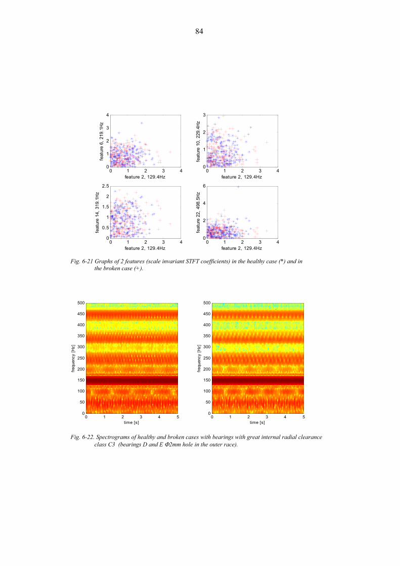
84

0 1 2 3 40

1

2

3

4

feature 2, 129.4Hz

feat

ure

6, 2

19.1

Hz

0 1 2 3 40

1

2

3

feature 2, 129.4Hz

feat

ure

10, 2

29.4

Hz

0 1 2 3 40

0.5

1

1.5

2

2.5

feature 2, 129.4Hz

feat

ure

14, 3

19.1

Hz

0 1 2 3 40

2

4

6

feature 2, 129.4Hz

feat

ure

22, 4

98.5

Hz

Fig. 6-21 Graphs of 2 features (scale invariant STFT coefficients) in the healthy case (*) and in

the broken case (+).

frequ

ency

[Hz]

time [s]0 1 2 3 4 5

0

50

100

150

200

250

300

350

400

450

500

frequ

ency

[Hz]

time [s]0 1 2 3 4 5

0

50

100

150

200

250

300

350

400

450

500

Fig. 6-22. Spectrograms of healthy and broken cases with bearings with great internal radial clearance

class C3 (bearings D and E Φ2mm hole in the outer race).

85

0 20 40 60 80 1000

100

200

300

400

500

600

Mahalanobis distances

Num

ber o

f sam

ples

>

Fig. 6-23 Distributions of the Mahalanobis distances between a learning set (yellow dotted line with cir-cles) and the feature vectors of test sets of 5120 samples. The learning set is of healthy case, bearing D (clearance class C3). The blue dot line with circles is the distribution for a healthy test set and the thin solid lines are the distributions for broken case test sets (bearing E, clear-ance class C3, Φ2mm hole in outer race).

0 20 40 60 80 1000

100

200

300

400

500

600

Mahalanobis distances

Num

ber o

f sam

ples

>

Fig. 6-24 Distributions of the Mahalanobis distances between a learning set (yellow dotted line with cir-cles) and the feature vectors of test sets of 5120 samples. The learning set is for a healthy case, bearing A (clearance class ‘normal’). The blue dotted line with circles is a distribution for a healthy test set and thin solid lines are the distributions for broken case test sets (bearing E, clearance class C3, Φ2mm hole in the outer race).

86

0 20 40 60 80 1000

100

200

300

400

500

600

Mahalanobis distances

Num

ber o

f sam

ples

>

Fig. 6-26. Distributions of the Mahalanobis distances between a learning set and the feature vectors of

test sets of 5120 samples. The learning set (yellow dotted line with circles) is of healthy case, bearing A (clearance class ‘normal’). The green dotted line with circles is a distribution for a healthy test set (bearing A), solid lines without markers are the distributions for healthy case test sets ( bearing D, clearance class C3) and solid lines with plus signs are the distributions for healthy case test set (bearing F, clearance class C4).

0 20 40 60 80 1000

100

200

300

400

500

600

Mahalanobis distances

Num

ber o

f sam

ples

>

Fig. 6-25. Distribution of the Mahalanobis distances betweena a lerning set (yellow dotted line with cir-

cles) and the feature vectors of test sets of 5120 samples. The learning set is for a healthy case (bearing F, clearance class C4). The green dotted line with circles is a distribution for a healthy test set and thin solid lines are the distributions for broken case test sets (bearing G, clearance class C4, φ2mm hole in the outer race).

87

0 20 40 60 80 1000

100

200

300

400

500

600

Mahalanobis distances

Num

ber o

f sam

ples

>

Fig. 6-27. Distributions of the Mahalanobis distances between a learning set (yellow dotted line with

circles) and the feature vectors of test sets of 5120 samples. The learning set is for a healthy case, bearing D (clearance class C3). The green dotted line with circles is a distribution for a healthy test set (bearing D), solid lines without markers are the distributions for broken test sets (bearing E, clearance class C3, Φ2mm hole in the outer race) and solid lines with plus signs are the distributions for healthy case test sets (bearing F, clearance class C4).

1.5 2 2.5 38

9

10

11

12

feature 1, 557.8Hz

feat

ure

5, 4

56.5

Hz

1.5 2 2.5 32

4

6

8

feature 1, 557.8Hz

feat

ure

9, 3

55.2

Hz

1.5 2 2.5 30

5

10

15

feature 1, 557.8Hz

feat

ure

13, 2

52.6

Hz

1.5 2 2.5 30

2

4

6

8

feature 1, 557.8Hz

feat

ure

21, 1

85H

z

Fig. 6-28. Graphs of 2 features in the healthy case (*) and in the broken case (+) with bearings of internal radial clearance class C4. Feature 21 (185 Hz) is not a modulated frequency of the bearing pass frequency.

88

Table 6-8. Mean values of the Mahalanobis distances between a learning set and feature vectors of test sets. The number of single outliers exceeding 95% significance level were calculated using F-distribution (Equation 4.17). Values are calculated using 5120 feature vectors in each group. The critical Mahalanobis distance producing a confidence interval of 95% is CR= 63.5.

row learning set test set µ(r) > CR 95%1 A A 42.4 2762 A B 104.3 5333 A B 175.4 8124 A B 98.4 3575 A B 61.2 3176 A C 35.8 2667 A C 26.5 1628 A C 63.7 6969 D D 27.9 150

10 D E 36.7 36211 A E 104.5 505912 A E 88.5 506713 F F 23.8 3914 F G 143.7 497815 F G 126.8 476216 F G 453.7 511817 F G 148.1 510018 A D 98.9 508119 A D 119.1 509520 A F 99.1 512021 A F 90.7 5118

bearing

0 100 200 300 400 500 600 700 8000

0.001

0.002

0.003

0.004

0.005

0.006

0.007

0.008

0.009

0.01

taajuus [Hz] 0 200 400 600 800 1000 1200

0

0.1

0.2

0.3

0.4

0.5

0.6

0.7

0.8

0.9

1

taajuus [Hz]

Fig. 6-29. The envelope spectra of the vibration signal obtained with the piezoelectric accelerometer. Motor at no load. The spectrum of bearing A (clearance class ‘normal’) is in the left figure and spectrum of bearing B (clearance class ‘normal’, Φ2mm hole in the outer race) is in the right figure. The ball pass frequency is 91.8 Hz.

89

0 20 40 60 80 1000

100

200

300

400

500

600

Mahalanobis distances

Num

ber o

f sam

ples

>

Fig. 6-30. Distributions of the Mahalanobis distances between a learning set and the feature

vectors of test sets of 5120 samples (bearings with clearance class ‘normal’). The learning set (yellow dotted line) is for a healthy case, bearing A. The green dotted line is a distribution for a healthy test set and thin solid lines are the distributions for bro-ken case test sets (bearing B, Φ2mm hole in outer race). The motor is under no load condition.

0 20 40 60 80 1000

100

200

300

400

500

600

Mahalanobis distances

Num

ber o

f sam

ples

>

Fig. 6-31. Distributions of the Mahalanobis distances between a learning set and the feature

vectors of test sets of 5120 samples (bearings with clearance class C3). The learning set (yellow dotted line) is for a healthy case, bearing D. The green dotted line is a dis-tribution for a healthy test set and thin solid lines are the distributions for broken case test sets (bearing E,Φ2mm hole in the outer race ). Motor at no load.

90

0 20 40 60 80 1000

100

200

300

400

500

600

Mahalanobis distances

Num

ber o

f sam

ples

>

Fig. 6-32. Distributions of the Mahalanobis distances between a learning set and the feature vectors of

test sets of 5120 samples (clearance class C4). The learning set (yellow dotted line) is for a healthy case, bearing F. The green dotted line is a distribution for a healthy test set and thin solid lines are the distributions for broken case test sets (bearing G, Φ2mm hole in the outer race). Motor is at load.

Table 6-9. Mean values of Mahalanobis distances between learning set and feature vectors of test sets. Motor in no load condition. Number of single outliers exceeding 95% significance level calcu-lated using F-distribution (equation 4.17). Values are calculated using 5120 feature vectors in each group. The critical Mahalanobis distance producing the confidence interval of 95% is CR= 63.5.

row learning set test set µ(r) > CR 95%1 A A 41.3 5922 A B 29.7 2583 A B 31 3094 A B 20.6 175 A B 24.1 406 D D 40.5 5957 D E 101.3 19508 D E 157.1 26409 A E 284.6 5120

10 A E 320 512011 F F 27.8 7912 F G 138.9 263213 F G 48.4 40214 F G 48.8 47415 A D 231.9 512016 A D 296.4 5120

bearing

91

6.2.5 The optimisation of the time-frequency window for a detection of the bearing fault using a stator current signal

In the previous tests, all conditions except the damage of the bearing were kept as constant as possible. Under this condition, we can hypothesise that if the bearing damage changes the fre-quency components of the stator current, the difference between a healthy and broken case signal should be bigger at these frequencies than at any other frequencies. This is tested using the optimal Gabor- filter parameter selection described in Chapter 4.1.4. Unlike in the previous chapter, the method does not predefine any frequencies that should indicate a fault. Instead it searches for a kernel and frequency band combinations that maximises the distinctness of the classes.

The results of the optimisation are presented in Figures 6-33…6-38. First-Order statistics E1 (Equation 4.22) does not find the modulated bearing pass frequencies. It only finds the har-monic frequencies of the supply due to a normal slight variation in the motor load. Therefore, the results using discrimination energy E1 are not presented here. The hypothesis is incorrect if the mean energy of the frequency bands is the only measure of the difference.

The discrimination energy function E3 finds the maximum discrimination energy at a frequency of 201 Hz, the same value that was found with the averaged power spectrum of Figure 6-5. The hypothesis is incorrect again: there are frequency components that differ more than the bearing frequency components.

In Figure 6-33, the discrimination energy E2 (Equation 4.35) between the signals of healthy and broken cases (bearings A and B) has one peak at a frequency near 600 Hz. The peak is not near to the modulated bearing frequencies and the fact that there is only one peak indicates that it does not originate from the bearing pass impulse. On the other hand, the amplitude of the peak is much higher than in the case where two measurements from healthy case are compared (Fig-ure 6-34). This difference remains inexplicable (no explanatory factor found).

The discrimination energy E2 was calculated between signals measured in the cases where the motor was equipped with bearings of larger internal radial clearance. With the bearings with the internal radial clearance class C3 (Figures 6-35 and 6-36) some measurement files produced large discrimination energy E2 between a healthy and the broken case but for many files the discrimination energy remained as low as between healthy cases. In the case of bearings with the internal radial clearance class C4, the peaks were found to be near to the calculated frequen-cies and, as expected, the peaks were repeated with intervals in the bearing pass frequency (Figures 6-37 and 6-38). The results clearly support the results presented earlier in this thesis where bearing damage was found and classified reliably in the cases where the motor was equipped with the bearings of large internal clearance C4. The results also indicate that the discrimination energy E2 can find the most significant differences in the frequency spectra of signals even if the changes are very faint. The hypothesis is true when C4 bearings are used and the appropriate discrimination energy function is used to measure the difference between sig-nals.

Using second-order statistics some of the modulated bearing frequencies can be found. Even using this optimised Gabor filter the classification error was between 25%-50%. It is also im-portant to notice that this classification error was obtained, when training samples from both healthy and broken cases were used, which is not the practical case.

92

It is also important to notice that all three discrimination energy functions E1, E2 and E3 find different features of signals. E1 finds the optimum filter for the separation based on the total energy of the frequency bands (mean values). The discrimination energy functions E2 and E3 produce probability distributions where the variances in the frequency contents are taken into account. However, the discrimination energy functions measure the distance between distribu-tions differently and therefore the bands that produce maximum differences between signals vary also. In addition, the length of the signals in the calculations affects on the variance values of Equations 4.28 and 4.29 and therefore the optimisation results. With this method, however, the differences were found on the same bands as with the averaged power spectrum method (Chapter 6.2.1). Also some of the modulated bearing pass frequencies fib (Equation 3.28) were found. Therefore, it is found to be a useful tool for the analysis of the differences in frequency contents of signals of two separate classes. However, the convergence problem arose with dis-crimination energy function E2 making it hard to find an optimum Gabor filter size. The problem is partly due to calculation method but also, it seems that the detection of a bearing fault using a stator current signal, when the bearing pass frequencies are found, is not very sen-sitive to the time-frequency window size.

0 200 400 600 800 1000 12000

2000

4000

6000

8000

10000

12000

E2

frequency [Hz]

Fig. 6-33. E2 discrimination energy curve between measurement files for a healthy case (bearing A) and a

broken case (bearing B). Bearings are of the internal radial clearance class ‘normal’.

93

0 200 400 600 800 1000 12000

10

20

30

40

50

60

70

80

90

E2

frequency [Hz]

Fig. 6-34. E2 discrimination energy curve between measurement files for healthy cases (bearing A). The

bearing is of the internal radial clearance class ‘normal’.

0 200 400 600 800 1000 12000

20

40

60

80

100

120

E2

frequency [Hz]0 200 400 600 800 1000 1200

0

0.5

1

1.5

2

2.5

3

3.5x 104

E2

frequency [Hz]

Fig. 6-35. E2 discrimination energy curves between measurement files for a healthy case (bearing D) and a broken case (bearing E). Bearings are of the internal radial clearance class C3. Left and the right side curves from separate measurement files.

94

0 200 400 600 800 1000 12000

10

20

30

40

50

60

70

80

90

E2

frequency [Hz]

Fig. 6-36. E2 discrimination energy curve between measurement files for healthy cases (bearing D). The

bearing is of the internal radial clearance class C3.

0 200 400 600 800 1000 12000

2000

4000

6000

8000

10000

12000

14000

E2

frequency [Hz]

Fig. 6-37. E2 discrimination energy curve between measurement files for a healthy case (bearing F) and a

broken case (bearing G). Bearings are of the internal radial clearance class C4.

95

0 200 400 600 800 1000 12000

2000

4000

6000

8000

10000

12000

E2

frequency [Hz]

Fig. 6-38. E2 discrimination energy curve between measurement files for healthy cases (bearing F, inter-

nal radial clearance class C4).

6.3 Conclusions

In this chapter (6), the feasibility of the stator current measurement as a bearing fault indicator was experimentally tested. In the first test, a standstill motor was magnetised with direct current and radial movements of the rotor were produced in order to achieve information on the stator current transient induction. The power spectrum estimates of the stator current signals were compared in the healthy and broken bearing cases and no significant differences between cases were found. The time-frequency representations of stator signals were classified with the Maha-lanobis distance calculation and the feasibility of the method was tested with artificially created test signal.

It was shown with the DC-magnetization test that the radial movement of the rotor induces stator current transient in the usual grid conditions (Table 6-1). On the other hand, the magni-tude of the current was very small if the radial movement was restricted with a bearing of small radial clearance (Table 6-2 and Figures 6-3 and 6-4). Simulation was used to show that the classification based on Mahalanobis distance is possible if radial movement at bearing pass frequency is present but that noise in the measurement chain and the non-sinusoidal time vary-ing air gap flux can prevent the indication of a fault. This is concluded from Table 6-6 and Figure 6-11 by comparing the classification results with different noise levels.

The outer race defect was clearly indicated only in the case of the large internal radial clearance of the bearing (internal radial clearance class C4 bearings. Normal wear (=large clearance) could not be distinguished from the bearing damage. This was tested using bearings of different internal radial clearance classes in calculations as presented in Tables 6-8 and 6-9.

The large internal radial clearance allows big radial movement of the rotor. On the other hand, a tendency to the radial movement of the rotor is affected by the magnetic pull between the rotor and the stator. In an ideal situation the value of this pull is zero. The magnetic pull is increased with the degree of the rotor eccentricity. The free eccentricity is increased if the radial clearance of bearing is great. This free eccentricity can rotate parallel to the maximum air gap flux density

96

causing the biggest possible force in the direction of the maximum flux causing the biggest change in stator current. In addition, load eccentricity can affect the size and the direction of the radial movement of the rotor.

In many researches the stator current signal has been found feasible in bearing fault monitoring. In this research, it was found that internal radial clearance has significant influence on the clas-sification possibilities. This result may explain also the different conclusion. In most experiments of others, tested motors have been relatively small. For example in the experiment of reference (Yazici, 1999) a ¾ HP induction motor was tested. In such a small induction motor, the ratio between the internal radial clearance of the bearing and the air gap length is greater than in the case of a bigger motor. Also, a smaller diameter of a rolling element of the bearing allows greater movement of the rotor for the same size of the hole in a bearing race. These fac-tors may lead to bigger stator current transient than the ones found in this research.

Also, as stated in Chapter 3.1.1 the rotating air gap flux is not the only modulating factor affect-ing on the vibration frequencies. Therefore, for example the forced dynamic eccentricity and consequent UMP modulates the vibration signal at the rotational frequency of the rotor. Even in this case there should exist the current components at the frequencies calculated by Equation 3.28 using the line frequency f as a modulator. However, the existence of these components is weakened and there exist the frequency components at other frequencies when the modulating frequency is rotational frequency fr or the frequency f x fr . The new modulator frequencies make the analysis even more unreliable.

One remark is that the estimation error between the calculated and the actual bearing frequency makes it hard to select frequency bands for feature vectors. In this experiment, a maximum error of 4% was found. To cover the correct band it would in this case require 15 frequency strips of 0.6 Hz, which in turn would enlarge the feature space and make it hard to distinguish the difference between a healthy and broken case even if the change existed.

With motors, where the stator current based bearing fault detection is possible, if any, the method has two further restrictions. Firstly, non-cyclic faults cannot be indicated and, secondly, the method can be hardly used with frequency converter driven motors, because of the distorted current waveform.

The main conclusion is that the stator current measurement as a bearing fault indicator is not adequate in the case of a 15 kW 4-pole motor with the bearing with normal radial clearance.

A feasibility of the stator current measurement as a bearing fault indicator is questionable in practical condition monitoring where high reliability of the analysis is required. For this reason, the measurement of the radial movement of the rotor, the measurement of vibration or acoustic emission is needed.

97

7. MICROMACHINED SILICON ACCELEROMETER

As concluded in the previous chapter, it is practically impossible to detect bearing faults with stator current based analyses. On the other hand, vibration monitoring is largely used in a bear-ing condition monitoring and has proved its reliability in practical systems. Spectrum analysis of a conventional piezo-electric accelerometer signal is the most commonly used procedure. Standard piezoelectric accelerometers with auxiliary electronics are still, despite decreasing prices, relatively expensive devices. Two different ways can be used to reduce the price of the bearing monitoring device. One is to use the calculation and communication capabilities of other devices such as motor protection relays. Another way is to use cheaper accelerometers than today. When all signal conditioning circuits are integrated in accelerometer chip, the sim-plicity of the system increases and cheaper products can be developed. There exist piezoelectric and piezo- resistive sensors that are packed with amplifiers and temperature sensor in one pack-age. Another solution is the use of MEMS chips (Micromachined Elctromechanical System) in which the accelerometer is one part of an integrated silicon chip. Development of cheap mi-cromachined chips (MEMS) has been rapid recently. Despite the poorer performance of micromachined sensors compared to piezoelectric devices they can offer the cheaper alternative in condition monitoring with possible restrictions set by ambient factors and by the capability to measure very small and very large vibration levels. If the performance of the integrated circuits with micromachined accelerometer is adequate, cheap means to construct vibration analysis device are provided because A) MEMS chips are cheap, B) amount of auxiliary electronics is lesser than with piezoelectric sensors and C) many micromachined accelerometers include tem-perature sensor on chip.

In this chapter, the advantages and the disadvantages of micromachined accelerometers are presented and the performance in bearing condition monitoring is evaluated. The characteristics of traditional piezoelectric sensors and capacitive micromachined sensors are presented and the effects of features and performance limitations on condition monitoring of bearings of electric motors are discussed. The performances of the micromachined chip and piezoelectric sensors are compared when an envelope spectrum method is used. The characteristics of micro-machined sensors are discussed in many papers but they do not consider condition monitoring and especially not the envelope spectrum method (Mohd-Yasin, 2001), (Lindh, 2002c).

7.1 Characteristics of conventional piezoelectric sensors and micro-machined sensors

Principle of operation. The micromachined accelerometer in most cases is capasitive, piezore-sistive or piezoelectric. In this study the capacitive type of accelerometer is used. The chip consists of a micromachined capacitor and amplifier. The capacitive element of the accelerome-ter chip consists of electrodes connected to a frame and to a moving mass, and of a flexible membrane between them. Acceleration is sensed with the measurement of the capacitance be-tween the moving mass and the supporting frame. Thus the structure of the sensor element of the capacitive micromachined accelerometer is a spring-mass-damper system that can be de-scribed by an ordinary linear 2. order differential equation. The construction and the fabrication process have great influence on the parameters and thus on mechanical properties of the accel-erometer. These factors determine directly the mechanical Brownian noise of the accelerometer. Electronics in combination with the sensitivity of the accelerator determines the electrical noise. The sensitivity in turn is dependent on mechanical structure. It is possible to construct a very low noise accelerometer under these restrictions. In a laboratory environment, Bernstein et. al.

98

(1999) have constructed a capacitive silicon accelerometer with a bandwidth of 10 kHz that has a noise level of 1.5 µg/√Hz. This indicates that reduction in the noise level is expected in indus-trially fabricated devices also. (Theoretical mechanical Brownian noise limit is less than 0.5 µg/√Hz).

A conventional piezo-electric capacitor is accurate, sensitive and its frequency range is ade-quate for the vibration monitoring of electric motors. The size and the price of the devices are bigger than the ones of the micromachined silicon accelerometer. Also the amount of the re-quired auxiliary electronics is bigger, in practice.

The characteristics of the tested sensors are given in Table 7-1. The noise level of the micro-machined ADXL105 sensor is approximately ten times larger than the noise level of the piezoelectric sensor. In condition monitoring of an induction motor bearing, signals of 3-5 kHz have to be measured. In this case, the amplitude range of the sensitive piezoelectric sensor can be from 2 mg up to 80 g (g=9.81m/s2) while the amplitude range of the micromachined sensor is approximately from 20 mg to 5 g.

Table 7-1. Characteristics of micromachined ADXL105 accelerometer chip and SKF CMSS786A piezo-electric accelerometer.

Sensor Frequency band Noise Sensitivity Measurement rangeSKF CMSS786A 0.5 … 14 000 Hz 20 mg/√Hz ,2 Hz 95-105 mV/g ±80g

AD ADXL105 0 … 12 000 Hz 225 mg/√Hz 225-275 mV/g ±5 g

The noise level of the micromachined sensor given in table (Ntyp) is corrected with the follow-ing equation

KfNN bwtypRMS = , (7-1)

where fbw is the used band and K is the constant dependent on the filter used (for 1. order, K=1.6). The measured RMS noise is 22 mg (g=9.81m/s2), when the band is limited with 1. order low pass filter with a cut-off frequency of 3 kHz (- 3dB). The calculated value according to Equation 7-1 is 22,5 mg.

0 20 40 60 80 100-80

-60

-40

-20

0

20

40

60

80

a [m

g]

t [ms]0 2 4 6 8 10

0

0.02

0.04

0.06

0.08

0.1

0.12

0.14

0.16

0.18

f [kHz]

a [m

g]

Fig. 7-1. Measured noise of ADXL105 accelerometer.

There exists micromachined silicon accelerometers for the higher acceleration ranges but their noise is too big and sensitivity too low for electric motor condition monitoring purposes. The tested accelerometer can in practice measure acceleration levels of 10 g, which is enough in

99

some applications. Crushers, propeller pumps for example on the other hand can cause accelera-tion levels of tens of g:s.

The normal maximum operational temperature of the tested micromachined accelerometer is 85 °C and the maximum temperature that does not cause permanent damage is 125 °C. The tem-perature of the chip is approximately the same as the ambient temperature because of the small power consumption (2 mW) and high heat conductivity of the case (30 °C/W). Maximum op-erational temperature of the conventional piezo-electric sensors can be more than 150 °C. The temperature limitations of the micromachined sensor can prevent the use of this type of sensor in some applications and at least affect the connection point on motor frame. In Table 7-2, IEC 85 insulation classes with maximum permissible temperatures of windings are presented. The motor frame temperature is however much lower than this. At 20 °C ambient temperature the frame temperature is often about 40-55 °C. The bearing temperature rise from the frame tem-perature is about 10-25 °C (D-end). However, when the motor is overloaded, the bearing temperature can easily rise up to more than 100 °C. On the other hand, the maximum allowable running temperature of the grease lubricated rolling element bearing is approximately 100 °C with a standard lubricant (Bonnet, 1992b).

Table 7-2. Maximum winding temperatures and maximum permissible temperature rises of insulation classes according IEC 85

Class Winding Temp. Temperature riseA 105 °C 60 °CB 130 °C 80 °CF 155 °C 105 °CH 180 °C 125 °C

The frequency characteristics differ remarkably between a micromachined accelerometer ADXL105 and a piezo-electric accelerometer CMSS786A. The resonance frequency of the ADXL105 is at 5 kHz if the chip is not glued and at 8 kHz if the chip is glued to circuit board. The resonance amplification is less than 10 dB. Above 10 kHz the attenuation increases rapidly. The piezo-electric accelerometer CMSS786A has a flat frequency response up to 14 kHz from where the amplification increases to +3 dB at 20 kHz.

7.2 Measurement apparatus

Measurements were taken with the testing equipment described in Chapter 5. Measurements were done with a piezoelectric and micromachined capacitive sensor installed parallel on the motor frame. Signals from the piezo-electric sensor were anti-aliasing filtered as described in Chapter 5. The micromachined sensor was tested with and without an anti-aliasing filter. The measurement configuration is illustrated in Figure 7-2. The measurement chain of the piezoelectric sensor SKF CMSS768A is described in Chapter 5. The micromachined sensor (type ADXL105) was manufactured by Analog Devices Inc. The test chip was soldered to a printed circuit board (Figure 7-3). The signal was filtered with a first order low pass filter that had a cut off frequency (–3dB) of 3kHz. The sampling frequency of the AD-conversion of both signals was 20kHz. The signals were collected with the data acquisition card. Envelope spectra of the signals were constructed with Matlab™ -program. Spectrum components characteristic to a fault were analysed visually.

100

MMDC Drive

DC Motor Induction Motor3 Phase Supply400V 50Hz

Database

3 Phase Supply400V 50Hz

Piezo-electricaccelerometer

Torque and RPM Meters

DisplayUnit

Amplifier

Anti Aliasing Filter

AD Converter

Filter

Micromachinedaccelerometer

Fig. 7-2. Measurement configuration for bearing damage detection using a micromachined

capacitive accelerometer.

Fig. 7-3. The micromachined capacitive accelerometer soldered on a printed circuit board.

7.3 Measurements

Measurements were taken with all bearings in Table 5-1,when the motor was at full load and at no load. The sampling frequency was 20 kHz or 30 kHz in some of the measurements.

The power spectrum (0-1 kHz) of the signal from the micromachined chip ADXL105 is pre-sented in Figure 7-4. The motor is in full load condition and equipped with bearing B (clearance class ‘normal, Φ2mm hole in the outer race). No bearing pass frequency can be found from spectrum directly. Further, the power spectra of piezoelectric sensor and micromachined sensor at the frequency band 0-10 kHz are presented in Figure 7-5. It is found that motor frame reso-nates at a frequency band 2-3 kHz. This band is used in the envelope spectrum analysis. The micromachined accelerometer resonates strongly at a frequency band 4-9 kHz. The resonance

101

does not affect the creation of the envelope spectrum if the amplitude of the acceleration is inside the measurement range of the accelerometer. Even if the amplitudes at resonance fre-quencies are bigger than the measurement range it is often possible to detect a bearing fault by the envelope spectrum. Of course, new frequency components arise in the spectrum but as far as the non-distorted fraction of the signal produce significantly more energy at the 2-3 kHz than distortion, the analysis is possible. By gluing the micromachined accelerometer to printed cir-cuit board the resonance frequency could be increased to 8 kHz. This is required in most cases since the resonance frequency of the motor frame is often up to 5 kHz.

0 100 200 300 400 500 600 700 800 900 1000-60

-50

-40

-30

-20

-10

0

10

frequency [Hz]

a [d

B]

Fig. 7-4. Power spectrum of the signal of micromachined accelerometer. The motor is at full load with broken bearing (B). The highest peaks are at frequencies 50,75,100,125,150,200,250, 300 Hz. No bearing pass frequency is visible.

0 2 4 6 8 10-50

-40

-30

-20

-10

0

10

20

f [kHz]

a (d

B)

piezo-electric accelerometer

0 2 4 6 8 10-25

-20

-15

-10

-5

0

5

10

15

f [kHz]

a (d

B)

micromachined accelerometer

Fig. 7-5. Power spectra of the signal of the piezo-electric accelerometer and micromachined accelerometer. The motor is at full load with broken bearing (B). Motor frame resonance is at 2-3kHz. The micro-machined accelerometer resonates in the frequency band 4-9 kHz.

102

7.3.1 Envelope spectra at no load

The motor was loaded with the DC-machine not connected to the grid. The signal of the mi-cromachined chip was not filtered. The creation of the envelope spectrum is presented in Figures 7-6 and 7-7. Figure 7-6 presents the spectrum from a measurement with healthy bearing A (radial clearance class ‘normal’) and Figure 7-7 with broken bearing B (radial clearance class ‘normal’, Φ2mm hole in the outer race).

0 0.05 0.1 0.15-6

-4

-2

0

2

4

6

a [g

]

a) measured acceleration t [s]0 2000 4000 6000 8000 10000

-100

-50

0

50

100

[dB

]

b) band pass filter f (Hz)

0 0.1 0.2 0.3 0.4 0.50

0.5

1

1.5

2

c) filtered signal t [s]0 100 200 300 400

0

0.02

0.04

0.06

0.08

0.1

d) envelope spectrum f [Hz]

Fig. 7-6. Envelope spectrum of the signal of the micromachined accelerator. The motor at no load is

equipped with healthy bearing (A).

103

0 0.05 0.1 0.15-6

-4

-2

0

2

4

6a

[g]

a) measured acceleration t [s]0 2000 4000 6000 8000 10000

-100

-50

0

50

100

[dB

]

b) band pass filter f (Hz)

0 0.1 0.2 0.3 0.4 0.50

0.5

1

1.5

2

c) filtered signal t [s]0 100 200 300 400

0

0.02

0.04

0.06

0.08

0.1

d) envelope spectrum f [Hz]

Fig. 7-7. Envelope spectrum of the signal of the micromachined accelerator. The motor at no load is equipped with broken bearing (B). The highest peak is at a bearing pass frequency of 90.7 Hz.

7.4 Envelope spectra at full load

The induction motor was loaded with a DC-motor in order to obtain a constant speed of 1473 RPM. The envelope spectra of signals of the micromachined accelerometer (Figure 7-8) and piezo-electric accelerometer (Figure 7-9) both reveal the bearing pass frequency 89.3 Hz. The calculated value according to Equation 3.1 gives the frequency of 89.7 Hz with the sliding fac-tor 0.96 (4% slide). The first peak is visible at a frequency of 24.5 Hz that corresponds to the rotational speed. Also the modulated rotational frequency side bands of the bearing pass fre-quency are visible as expected in Chapter 3.1.1. In Figure 7-10 the highest peak at 125 Hz is not a bearing pass frequency. This can be concluded without prior information by comparing this frequency with the calculated characteristic frequency, setting the trigger level that is above the peaks amplitude and finally, by searching the peaks at multiple frequencies and at their side band frequencies. Furthermore, if the envelope spectrum from the motor with a healthy bearing is recorded in a file (or memory), the change of the envelope spectrum evolving with time can be analysed.

104

0 0.02 0.04 0.06 0.08 0.1 0.12 0.14 0.16 0.18 0.2-2

-1

0

1

2

t [s]

a [g

]

0 50 100 150 200 250 300 350 400 450 5000

0.02

0.04

0.06

0.08

0.1

f [Hz]

Fig. 7-8. The signal of a micromachined accelerometer and its envelope spectrum when a motor with a broken bearing (B) is running at full load. The highest peak is at a bearing pass frequency of 89.3 Hz and at its multiples.

0 0.02 0.04 0.06 0.08 0.1 0.12 0.14 0.16 0.18 0.2-2

-1

0

1

2

t [s]

a [g

]

0 50 100 150 200 250 300 350 400 450 5000

0.002

0.004

0.006

0.008

0.01

f [Hz]

Fig. 7-9. The signal of a piezo-electric accelerometer and its envelope spectrum when a motor with a broken bearing (B) is running at full load. The highest peak is at a bearing pass frequency of 89.3 Hz and at its multiples.

105

0 0.02 0.04 0.06 0.08 0.1 0.12 0.14 0.16 0.18 0.2-2

-1

0

1

2

t [s]

a [g

]

0 50 100 150 200 250 300 350 400 450 5000

0.02

0.04

0.06

0.08

0.1

f [Hz]

Fig. 7-10. The signal of a micromachined accelerometer and its envelope spectrum when a motor with a healthy bearing (A) is running at full load. The highest peak is at the bearing pass frequency of 89.3 Hz and at its multiples.

The filtering of the output of the micromachined accelerometer with a 1. order low pass filter with a cut-off frequency at 3 kHz has almost no effect on the detection possibilities of the bear-ing fault (Figure 7-11). The filter removes components that are aliased from the frequencies above Nyquist frequency. However, the attenuation of the ADXL105 increases quickly above the frequency of 10 kHz so that the amplitudes of these aliased peaks are very low.

The spectrum of the signal with the bigger fault (bearing C , Φ5mm hole in the outer race) is presented in Figure 7-12. The spectra in the case of a motor with bearings with a larger internal radial clearance (C4) for a healthy case and in a broken case are presented in Figure 7-13. It is discovered that bearing fault detection is possible even when the acceleration level is bigger than the measurement range given by the accelerometer manufacturer. When the acceleration level increases even more, the amplitude of the output of the accelerometer is restricted and the fraction of the signal is cut off. In order to test this, the amplitude of measurement signal is artificially restricted below the RMS amplitude of the signal. The bearing pass frequency is still visible (Figure 7-14).

106

0 0.02 0.04 0.06 0.08 0.1 0.12 0.14 0.16 0.18 0.2-4

-2

0

2

4

t [s]

a [g

]

0 50 100 150 200 250 300 350 400 450 5000

0.05

0.1

0.15

0.2

f [Hz]

Fig. 7-11. The signal of a micromachined accelerometer with an anti-aliasing output filter and its enve-lope spectrum when a motor with a broken bearing (B) is running at full load. The highest peaks are at the rotational frequency and at the bearing pass frequency of 89.3 Hz and at its multiples. Calculated value with 4% slide is 89.1 Hz and with 0% slide is 92.8 Hz.

0 0.02 0.04 0.06 0.08 0.1 0.12 0.14 0.16 0.18 0.2

-5

0

5

t [s]

a [g

]

0 50 100 150 200 250 300 350 400 450 5000

0.1

0.2

0.3

0.4

f [Hz]

Fig. 7-12. The signal of a micromachined accelerometer and its envelope spectrum when a motor with a broken bearing (bearing C , Φ5mm hole in outer race) is running at full load. The highest peaks are at the rotational frequency and at the bearing pass frequency of 100 Hz and at its multiples. The calculated value with 4% slide is 99.0 Hz and with 0% slide is103.1 Hz.

107

0 50 100 150 200 250 300 350 400 450 5000

0.05

0.1

0.15

0.2

0.25

f [Hz]

0 50 100 150 200 250 300 350 400 450 5000

0.002

0.004

0.006

0.008

0.01

f [Hz]

Fig. 7-13. The envelope spectra of acceleration signals when the motor is running at full load with a healthy bearing (F, above) and broken bearing (G, below). Calculated value with 4% slide is 99.0 Hz and with 0% slide is103.1 Hz.

0 0.05 0.1 0.15-6

-4

-2

0

2

4

6

a [g

]

measured acceleration t [s]0 0.05 0.1 0.15

-6

-4

-2

0

2

4

6

a [g

]

amplitude restricted t [s]

0 50 100 150 200 250 300 350 400 450 5000

0.02

0.04

0.06

envelope spectrum f [Hz]

Fig. 7-14 The signal of a micromachined accelerometer and its envelope spectrum when a motor with a

broken bearing (G) is running at full load and the amplitude of the signal is cut. The bearing pass frequency still has the highest peak in the spectrum.

108

7.5 Conclusions

The envelope spectrum method can be used with a micromachined sensor and relatively small faults can be diagnosed. The detection of the most incipient faults (frame response <10mg) that can be found using the piezoelectric sensor is not possible due to the bigger noise level of the micromachined accelerometer. On the other hand, if the dominant vibration is big (crushers, cavitating pumps, piston compressors etc.) the amplitude range of the micromachined acceler-ometer is not adequate. However, the measurement range given in the manufacturer datasheet can be exceeded because the amplitude of the peaks has little effect on the bearing defect analy-sis based on the envelope spectrum.

A rather limited operational temperature range of the micromachined silicon accelerometer restricts its use in applications where very cold or hot temperatures appear.

109

8. AUTOMATIC ANALYSIS OF AN ACCELERATION SIGNAL

In this chapter, different methods to create features that are able to classify between a healthy and broken bearing are compared. The classification possibilities are also compared bearing in mind the restrictions of embedded devices and communications infrastructure of industrial plants. Two different pilot implementations and approaches to the integration of sensor, analy-ses and communications are presented.

Automatic analysis of an acceleration signal requires A) a sensor that can collect the data and make the analysis or deliver the data to another analysing device, B) data communications be-tween sensor and computers at higher levels in industrial communications infrastructure and C) analysis methods that can classify the measurement signal to be from a healthy or broken case. Two types of a sensor solutions are tested in this chapter: the first one is a sensor with a calcula-tion capacity for example for the production of the envelope spectra; the other one can collect the measurement data in the memory and another device can read the data via a field bus. The data communications requirements highly depend on the type of sensor solution selected. If the data is already analysed in the sensor the data communications are needed only for the results but in the other case, all measurement data needs to be transferred. The complexity of the classi-fication method can be great if the data is analysed with the management level computer, but if the analysis is made in the sensor itself, the analyses must be simple due to the restricted calcu-lation and memory capacity.

8.1 Feature extraction

The features can be extracted from the acceleration signal in many different ways. What is common for all of these is the source of information: The response of the motor frame to the bearing impulses. Excluding the stress wave techniques that utilise the response at several hun-dreds of kilohertz, the information can be obtained at a few kilohertz resonance range of the frame. In addition, the information of total amplitude of the acceleration is useful as a part of the analyses of the cyclic bearing faults and is often required for the indication of non-cyclic faults. The efficiency of feature extraction using envelope spectrum method, envelope autocor-relation method (Wang, 1996) and autocorrelation of joint time-frequency components are compared. Also, the envelope detection (demodulation) using a Gabor filter (STFT), digital pass band demodulation and Hilbert transform approach is compared.

8.1.1 Autocorrelation of a time-frequency presentation of a signal

As seen in Figures 3-4 and 4-2, the periodic bearing pass response is detectable at a wide fre-quency range of time-frequency representations. In this thesis, the time-frequency representation is formed using the STFT transform, because it reveals the bearing pass fre-quency and requires less calculation time than other time-frequency transforms. The procedure is as follows: the STFT coefficients of the acceleration signal are calculated for the desired centre frequency using Gabor filter of Equation 4.19. Then the autocorrelation of these coeffi-cients is calculated.

In Figure 8-1, the normalised autocorrelation sequences of STFT coefficients are presented for the healthy and broken cases. The bearing pass interval is visible and clear. In the case of small fault (bearing B), the results vary between samples. In Figure 8-2 the left diagram describes the

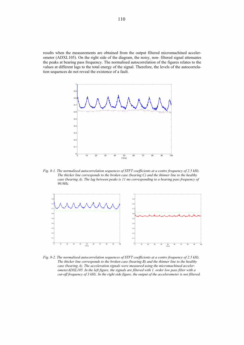
110

results when the measurements are obtained from the output filtered micromachined acceler-ometer (ADXL105). On the right side of the diagram, the noisy, non- filtered signal attenuates the peaks at bearing pass frequency. The normalised autocorrelation of the figures relates to the values at different lags to the total energy of the signal. Therefore, the levels of the autocorrela-tion sequences do not reveal the existence of a fault.

0 10 20 30 40 50 60 70 80 90 1000

0.1

0.2

0.3

0.4

0.5

0.6

0.7

0.8

0.9

1

t [ms]

Fig. 8-1. The normalised autocorrelation sequences of STFT coefficients at a centre frequency of 2.5 kHz. The thicker line corresponds to the broken case (bearing C) and the thinner line to the healthy case (bearing A). The lag between peaks is 11 ms corresponding to a bearing pass frequency of 90.9Hz.

0 10 20 30 40 50 60 70 80 90 1000

0.1

0.2

0.3

0.4

0.5

0.6

0.7

0.8

0.9

1

t [ms]0 10 20 30 40 50 60 70 80 90 100

0

0.1

0.2

0.3

0.4

0.5

0.6

0.7

0.8

0.9

1

t [ms]

Fig. 8-2. The normalised autocorrelation sequences of STFT coefficients at a centre frequency of 2.5 kHz. The thicker line corresponds to the broken case (bearing B) and the thinner line to the healthy case (bearing A). The acceleration signals were measured using the micromachined acceler-ometerADXL105. In the left figure, the signals are filtered with 1. order low pass filter with a cut-off frequency of 3 kHz. In the right side figure, the output of the accelerometer is not filtered.

111

8.1.2 Envelope autocorrelation method.

The envelope autocorrelation technique for the ball bearing defect detection is presented i.e. in (Wang, 1996). The detection of an envelope (or demodulation) can be done with several differ-ent procedures. The most usual way is to rectify and filter the signal as described in chapter 3.1.2 or to use Fourier-methods as described previously in Chapter 8.1.1. Other possibilities include wavelets (Nikolaou, 2002) or Hilbert transform (Wang, 1996), (Kang, 2002).

The procedure of the envelope autocorrelation is the following: the signal is band pass filtered in order to extract the motor frame resonance, then the signal is demodulated and the autocorre-lation is calculated. In this, the unbiased normalised autocorrelation is used. The envelope of the real valued signal is the absolute value of analytic signal (|z(t)| using Equation 4.5). In Fig-ure 8-3 the demodulation is performed with the analytic signal formation according to Equation 4.5.

0 20 40 60 80 1000

0.2

0.4

0.6

0.8

1

t [ms]0 20 40 60 80 100

0

0.2

0.4

0.6

0.8

1

t [ms]

0 200 400 600-100

-80

-60

-40

-20

0

20

f [Hz]

(dB

)

0 200 400 600-100

-80

-60

-40

-20

0

20

f [Hz]

(dB

)

Fig. 8-3. The envelope autocorrelations of a broken bearing case (left) and a healthy bearing case (right)

with C4 internal radial clearance class bearings (bearing F and bearing G, Φ2mm hole in outer race). The normalised autocorrelation sequences of the analytic acceleration signals are pre-sented in upper figures. The power spectrum estimate of the autocorrelation reveals the bearing pass frequency with rotational frequency sidebands in the bottom left figure.

Kang (2002) has proposed the Hilbert transform for envelope detection (demodulation) of vi-brational deflection shapes. With this method the information of the impulse response frequency is not needed and it is not required to band pass filter the resonance before demodula-tion in the case of sinusoidally excited structure.

In the case of automatic analysis of the acceleration signal it is important that human made adjustments are avoided. The natural frame frequencies vary between different motors. There-fore, if the analyses can be made without the selection of band pass filtering parameters the

112

implementation is more robust than in the cases where the band is selected or several bands are tested. On the other hand, the real world finite length version of the infinite length Hilbert trans-former of Equation 4.5 is not an ideal all pass filter. However, the pass band can be large for a relatively short filter (Proakis, 1996).

The applicability of the Hilbert transformer is tested in three tests. In the first test the autocorre-lation sequences are formed from the non-filtered, band pass filtered and Hilbert transformed acceleration signal. In the second test enveloping methods are compared. The methods include a Fourier transform based method, band pass method and Hilbert transformer method. In the third test, different Hilbert transformers, band pass filters and peak detection are evaluated. The sec-ond and the third tests are presented in Chapter 8.1.3.

In Figure 8-4 the autocorrelation sequences of the acceleration signal of the motor with the broken bearing are presented. The autocorrelation sequence in the subplot a) is calculated using the measured rectified signal directly. In the sequence b) the signal is first band pass filtered (pass band 2kHz-5kHz) then rectified before the autocorrelation calculation. The sequence c) is the autocorrelation of the absolute value of the analytic signal and the sequence d) is similar but the measurement signal is band pass filtered before the formation of an analytic signal. The bearing pass frequency is readable in every sequence. If autocorrelation of the acceleration signal is calculated, the use of an analytical signal is not useful since it does not enlarge the autocorrelation at lags describing the bearing fault. Whereas the band pass filter reduces the noise of the signal and makes the analysis easier at least in the case of visual inspection.

0 20 40 60 80 1000.5

0.6

0.7

0.8

0.9

1c) AC of non-filtered analytic signal

t [ms]0 20 40 60 80 100

0.5

0.6

0.7

0.8

0.9

1d) AC of band pass-filtered analytic signal

t [ms]

0 20 40 60 80 1000.5

0.6

0.7

0.8

0.9

1a) AC of non-filtered real signal

t [ms]0 20 40 60 80 100

0.5

0.6

0.7

0.8

0.9

1b) AC of band pass-filtered real signal

t [ms]

Fig. 8-4. Autocorrelation sequences of an acceleration signal of a motor with a broken bearing. The bear-ing pass frequency is readable in every sequence. Sequence a is calculated for the rectified measured signal directly. For sequence b the signal is first band pass filtered (pass band 2kHz-5kHz) then rectified before the autocorrelation calculation. Sequence c is the autocorrelation of the absolute value of an analytic signal and sequence d is similar but the real signal is firstly band pass filtered.

113

8.1.3 Envelope detectors for the envelope spectrum method

In this chapter envelope detectors are tested in conjunction with the envelope spectrum method. The envelope detectors tested are the Fourier method with a Gabor- filter implementation, the Hilbert transformer and the band pass filter. Also the peak detector using a median filter is tested.

The schemas of the actual envelope detectors used in the tests are illustrated in Figure 8-5. En-velopes are detected with a band pass demodulation (Figure a), with a Gabor-filter (Figure b) and with a Hilbert transformer (analytic signal) (Figure c). The band pass demodulation proce-dure filters the natural frame frequency with two 30. order Butterworth filters forming a pass band of 2-5 kHz. The filtered signal is rectified then decimated with a 2-phase decimator from sampling frequency of 20 kHz to a sampling frequency of 1.67 kHz. 2048- point FFT is calcu-lated for the power spectral estimate (periodogram method). The peak detector is otherwise similar to the band pass filter implementation but the band pass filter is replaced with a length ten median filter and peak selector. In Figure b, the Gabor filter uses the central frequency of 2.5 kHz. The magnitudes of the coefficients form a new time series that is low pass filtered and the power spectral estimate is formed as in the previous implementation. In the procedure of Figure c, the analytic signal is formed as a sum of the Hilbert transformer and the original signal according to Equation 4.19. The magnitude of the obtained complex signal is the signal enve-lope that is decimated and the PSD is formed as in other procedures.

s(n)D

4

D

3

|h(n)| FFT,PSD

s(n) FFT,PSD

Gs(n)

s(n)D

4

D

3

|h(n)| FFT,PSD

Hs(n) +

a)

b)

c)

Fig. 8-5. Envelope detection with a) a band pass demodulation, b) with a Gabor-filter and with c) a Hil-

bert transformer (analytic signal). The procedure a) filters the natural frame frequency with two Butterworth filters, then rectifies the signal and performs a 2-phase decimation (Fs/(3x4)). FFT is used for the calculation of the power spectral estimate (PSD). The procedure b) consists of a Ga-bor-filter, a low pass filter and an FFT-PSD block. In the procedure c) the analytic signal is formed as a sum of the Hilbert transformed and the original signal. The magnitude of the obtained complex signal is the signal envelope that is decimated and the PSD is formed as in procedure a.

114

In Figure 8-6 the envelope detection methods are compared. In the left side figures the enve-lopes using a) a band pass demodulation technique, c) a Gabor filter and e) an analytic signal are presented. The light curve is the original accelerometer signal, the dark line is the envelope. In the right side figures the power spectrum estimates of envelopes are presented. Although all of the methods reveal a bearing pass frequency of 99.8 Hz, the signal to noise ratio in the spec-trum from the Gabor filter based detection (Figure d) is lower that in the spectra from the band pass detection (Figure b) or from Hilbert transform based detection.

In Figure 8-7, the signal and its envelope is formed using a rectifier with several pass bands and an analytic signal. With narrow bands (band width from 2 to 3 kHz) the results are highly de-pendent on selected frequency band. The use of a wider band attenuates the spectrum components slightly compared to correctly selected narrow band or to Hilbert transformer based envelope spectrum. In this test, the Hilbert transformer produces the best ratio between the noise and the bearing pass frequency components. However, all of the previous tests with a Hilbert transformer (and analytic signal) were made with a quite complex algorithm that trans-forms a signal into the frequency domain, multiplies the obtained coefficients with the corresponding Hilbert filter coefficients and performs the inverse FFT. Fortunately, the Hilbert-transformers can be approximated with relatively short FIR or IIR filters when the unity magni-tude amplification is required only for a restricted band. For example, a 31 order Hilbert transformer FIR filter (Remez) for the pass band 1-9 kHz (Fs=20 kHz) can detect the envelope as well as a well tuned band pass filter and better than a wide band pass band filter. This is presented in Figure 8-8 where envelope spectra are formed using a) wide band pass demodula-tion, 31. order FIR Hilbert filter demodulation and c) also the peak detection demodulation. The peak detection method can also find the bearing frequency but more noise components are pre-sent in the spectrum than in the spectra of the band pass filter based methods.

115

30 40 50 60 70-5

0

5a)

t [ms]

a [g

]

0 100 200 300-30

-20

-10

0

f [Hz]

(dB

/Hz)

b)

30 40 50 60 70-5

0

5c)

t [ms]

a [g

]

0 100 200 300-30

-20

-10

0

f [Hz]

(dB

/Hz)

d)

30 40 50 60 70-5

0

5e)

t [ms]

a [g

]

0 100 200 300-30

-20

-10

0

f [Hz]

(dB

/Hz)

f)

Fig. 8-6. Envelope detection using a) a band pass demodulation technique, c) a Gabor filter and e) an analytic signal. The light curve is the original acceleration signal, the dark line is its envelope. On the right side figures the power spectrum estimates of the envelopes are presented. All of the spectra reveal the bearing pass frequency of 99.8 Hz.

116

30 40 50 60 70-5

0

5a) band pass demod. envelope

t [ms]

a [g

]

0 100 200 300-30

-20

-10

0

f [Hz]

(dB

/Hz)

b) pass band 2-4 kHz

0 100 200 300-30

-20

-10

0

f [Hz]

(dB

/Hz)

c) pass band 5-8 kHz

0 100 200 300-30

-20

-10

0

f [Hz]

(dB

/Hz)

d) pass band 2-8 kHz

30 40 50 60 70-5

0

5e) Hilbert demod. envelope

t [ms]

a [g

]

0 100 200 300-30

-20

-10

0

f [Hz]

(dB

/Hz)

f) Hilbert demodulation

Fig. 8-7. Envelope spectra of band pass demodulation with different pass bands and envelope spectrum with Hilbert demodulation in the case of a small bearing fault. With narrow bands (2 or 3 kHz) the results are highly dependent on the selected frequency band. The use of a wider band attenuates the spectrum components slightly compared to correctly selected narrow band or to Hilbert trans-former based envelope spectrum.

117

30 40 50 60 70-5

0

5a) band pass demodulation

t [ms]

a [g

]

0 100 200 300-30

-20

-10

0

f [Hz]

(dB

/Hz)

b) pass band 2-8 kHz

30 40 50 60 70-5

0

5c) length 31 Hilbert (FIR)

t [ms]

a [g

]

0 100 200 300-30

-20

-10

0

f [Hz]

(dB

/Hz)

d) Hilbert FIR 1-9 kHz

30 40 50 60 70-5

0

5e) peak detection demodulation

t [ms]

a [g

]

0 100 200 300-30

-20

-10

0

f [Hz]

(dB

/Hz)

f)

Fig. 8-8. Envelope spectra of band pass demodulation with different pass bands and envelope spectrum

with Hilbert demodulation in the case of a small bearing fault. With narrow bands (2 or 3 kHz) the results are highly dependent on the selected frequency band. The use of a wider band attenu-ates the spectrum components slightly compared to correctly selected narrow band or to Hilbert transformer based envelope spectrum.

8.1.4 Conclusions concerning the feature extractors

The outer race defects were detected reliably with all of the above techniques. The best separa-tion between healthy and broken cases is obtained using an envelope autocorrelation method or an envelope spectrum method explained in Chapter 3.1.2 and tested in Chapters 7.3 and 7.4. Therefore, it is not meaningful to implement time-frequency representation based methods in embedded systems. The envelope spectrum method is a logical selection for implementation because it requires less calculation effort than the envelope autocorrelation methods. The ability to extract features, based on the tests, is almost as good using the envelope methods as using the envelope autocorrelation method. The envelope can be detected based on band pass demodula-tion technique or the Hilbert transform technique. The Hilbert-transformer demodulation suggests no priori knowledge of useful frame resonance frequency band and is therefore the most natural selection for the feature extractor for automatic cyclic bearing fault detection. However, the use of a wide (1-8kHz) band does not remarkably attenuate the envelope spec-trum components and is therefore a possible selection also.

118

8.2 Classification of features

As defined in Chapter 2.1.3 the classification of faults can be based on deterministic rules or non-deterministic (statistical in particular) properties of measurement signal. In this chapter, the guidelines for the statistical fault classification of the envelope spectrum components using the Mahalanobis distance and deterministic classification with multi valued fuzzy logic are pre-sented.

As presented in Chapter 4.1.2, the Mahalanobis metrics is superior in the cases where the fea-tures are dependent as is the case with the spectrum components of an acceleration signal. Based on the distance calculations and a minimum distance classifier, possibly with a trigger level for the distance from the healthy case, a fully automatic system can be constructed. The main problems are, firstly, how the prototypes of faulty spectra are created and, secondly, how the trigger levels from a healthy case representing the abnormal situation are selected. In addi-tion, the rotational speed of the motor must be taken into account in the system by assuming known operation conditions or by rotational speed adaptation of the spectrum. Being so that only the healthy case spectrum is available a priori knowledge of the faulty case patterns must be included in the system artificially. Another possibility is to use a broken case spectra ob-tained from another motor with a broken bearing.

The proposed system consists of the following training phase actions • The creation of artificial spectra for the cases of an outer race defect, an inner race de-

fect, a cage defect and a rolling element defect. • The creation of an over all acceleration level feature for low, normal, high, very high

levels of vibration. • Calculation of a normal case prototype vector using several measurements from a

healthy case.

And of test phase actions using statistical distance calculation • The minimum distance classification using the calculation of distance between a test

vector of healthy and all broken case prototype vectors. • Classification of abnormal versus normal using trigger level distances from a healthy

case vector.

Or/and test phase actions using fuzzy logic including • Calculation of memberships in the output sets that describe the degree of fault for

every fault type under consideration. • Calculation of memberships in the output sets that describe the correct classification

probability of fault for every fault type under consideration. • As a combination of the previous memberships, the selection between a healthy and

faulty case with fault type information and instructions for the action.

8.2.1 Classification using the Mahalanobis distance calculation and mini-mum distance classifier

A bearing fault feature vector consists of PSD components of a signal envelope at selected frequencies. The selected components represent the characteristic fault frequencies and their three nearest harmonic frequencies for all the following faults: outer race fault o, inner race

119

fault i, rolling element fault b and cage fault c. The frequencies are calculated according equa-tions 3.1-3.4. These PSD components X form a 16 dimensional feature vector as follows

[])4()3()2()()4()3(

)2()()4()3()2()()4()3()2()(

ccccbb

bbiiiioooo

fXfXfXfXfXfXfXfXfXfXfXfXfXfXfXfX=F

(8.1)

Also the procedure that analyses all the damages separately using only a four-dimensional fea-ture space is tested. The values of prototype vectors are selected to represent 40 different levels of failure. The impulse response of the motor frame to the bearing impulse is a series of resonat-ing waves as described in Chapter 3.1. The envelope of the vibration is not sinusoidal. Therefore, the harmonic waves of the bearing pass frequency are found in spectrum but are attenuated compared to the bearing pass frequency. The values of prototype vectors are selected bearing this in mind. The prototype vectors are done without testing their discrimination power using a big value for the characteristic frequency and then a smaller value to the harmonics in descending order. The features not influenced by a certain fault are set to one, the bearing pass frequency component to five, the first harmonic to four, the second to three and the third to two. Then the values are altered to represent 40 different levels of damage and 20 % random varia-tion is added to the values.

Formation of a test vector. From the envelope spectrum of real measurement the twelve compo-nents in the neighbourhood of the calculated characteristic frequency (frequency resolution of PSD ∆f ≈ 0.2 Hz) were selected for pre-processing, in which, the maximum value of these five was selected as a feature. Envelope spectra for the outer race fault were formed using actual measurements. In the case of other faults the spectra of the healthy case were altered artificially near characteristic frequencies.

Classification. In the first test the distance between both the test vector and the vectors repre-senting the different fault types of the healthy case were calculated according to Equation 4.11 using the jacknified Mahalanobis distance calculation. Then a minimum value was selected and the test vector was classified to belong to a corresponding class. In the second test the distances were calculated with reduced feature spaces so that only the features representing a certain fault class were selected to a feature vector. The distances between the four test vectors and the cor-responding fault prototypes as well as healthy class prototypes were calculated separately. If in one or more calculations the distance to a faulty class was less than to the healthy class the corresponding fault was classified. This procedure makes it possible to recognise multiple si-multaneous fault cases. On the other hand, the possibility of an incorrect estimate is greater than in previous test because the values not changing due to a fault are not taken into account (weaker covariance information).

Results. The envelope spectrum of a healthy motor is illustrated in the Figure 8-9 (upper dia-gram). The spectrum components that are selected for the test feature vector are marked with *. This vector is illustrated in the lower figure with the (mean) prototype vectors of fault classes. The corresponding curves in the case of the outer race fault and inner race fault are presented in Figures 8-10 and 8-11. The classification results are presented in Tables 8-1 and 8-2. Table 8-1 presents the classification results using a 16 dimensional feature space, covering all four fault types and Table 8-2 presents the classification results using four dimensional feature space. Both indicate only correct classification results. The statistical distance between healthy and broken cases is bigger when four- dimensional feature space is used. On the other hand, there is more chance of misclassification if the shape of the test feature vector change. It is important to

120

bear in mind, firstly, that the correct classification was obtained without any tuning of the proto-type vectors, and secondly, that there can be many other fault modes that were not taken into account and much more research work should be done with various fault types and motors be-fore jumping to conclusions that generalise the result obtained with these tests.

0 100 200 300 400 500 6000

1

2

3

4

5

6x 10-3

f [Hz]

0 2 4 6 8 10 12 14 160

1

2

3

4

5x 10-3

Outerrace

Innerrace

rollingelement

cage

testvector

features

Fig. 8-9. The envelope spectrum of a healthy motor is illustrated in the upper figure. The spectrum com-

ponents that are selected for the test feature vector are marked with *. This vector is illustrated in the lower figure with the prototype vectors of the outer race fault (∧ ), the inner race fault (∨ ), the ball spin fault (o ) and the cage fault ( ). The vector of healthy case is a unity vector.

121

0 100 200 300 400 500 6000

1

2

3

4

5

6x 10-3

f [Hz]

0 2 4 6 8 10 12 14 160

1

2

3

4

5

6x 10-3

Outerrace

Innerrace

rollingelement cage

testvector

features

Fig. 8-10. The envelope spectrum of a motor with an outer race faulted bearing is illustrated in the upper figure. The spectrum components that are selected for the test feature vector are marked with *. This vector is illustrated in the lower figure with the prototype vectors of the outer race fault (∧), the inner race fault (∨ ), the ball spin fault (o ) and the cage fault ( ). The vector of healthy case is a unity vector.

0 100 200 300 400 500 6000

1

2

3

4

5

6x 10-3

f [Hz]

0 2 4 6 8 10 12 14 160

2

4

6

8x 10-3

Outerrace

Innerrace

rollingelement

cage

testvector

features

Fig. 8-11. The envelope spectrum of a motor with an inner race faulted bearing is illustrated in the upper

figure and features are marked similarly as in the previous figure.

122

Table 8-1. Classification results using 16 dimensional feature space covering all four fault types. The bold cases are selected with the minimum distance classifier.

healthy outer race inner race ball spin cagehealthy 0.6981 1.3607 2.7905 1.6052 2.3892outer race 5.3817 1.2018 7.0394 8.7226 7.5465inner race 3.7498 5.5534 1.666 4.43 5.7718ball spin 6.5451 5.3318 8.2085 1.0579 6.7352cage 0.6952 0.883 1.1753 1.3041 0.2143

Table 8-2. Classification results using four dimensional feature space. The distance between test vector and any fault prototypes are calculated separately. The bold cases are selected with the minimum distance classifier.

test data distance to outer race inner race ball spin cagehealthy healthy 0.1767 0.148 0.1107 0.138

broken 0.781 4.235 1.2339 1.3203outer race healthy 3.9542 0.2946 0.2454 0.2164

broken 0.0394 6.5133 1.4492 1.4779inner race healthy 0.2531 2.0595 0.137 0.0961

broken 0.9665 0.7749 1.4533 1.5183ball spin healthy 0.2327 0.3109 4.4202 0.1176

broken 0.9328 4.1784 0.2219 1.7265cage healthy 0.2827 0.3915 0.2275 4.0238

broken 1.0563 5.0148 1.7709 0.073

8.2.2 Classification using fuzzy logic

The advantages of the fuzzy logic approach include the possibility to change the linguistic rules into decisions copying the procedure and thinking of a human analyser. The rules that include uncertainty and inaccuracy are changed into numbers describing the severity of the fault or the probability of a fault. The rules and membership functions can be tuned so that the sensitivity of the system is good. On the other hand, when the fuzzy logic requires tuning of parameters, it is possible that it is tuned to find faults from test data, but the logic remains case specific. In this thesis, the purpose of introducing fuzzy logic is to demonstrate its possibilities as part of an automatic fault classification; the purpose is not to tune parameters in order to maximise the reliability of the system. The fuzzy logic has been used in machinery vibration analysis by for example Mechefske (1998).

In order to demonstrate the applicability of fuzzy logic two different models are created. The first model uses the 16 dimensional feature vectors presented in the previous chapter. Features of each fault type are tested separately. Therefore, the inputs include the magnitudes of the envelope spectrum components at the expected ball pass frequency and their three nearest har-monic frequencies separately for all the following faults: outer race fault o, inner race fault i, rolling element fault b and cage fault c. The input sets consist of the sets low, medium, high and very high. The membership functions are triangle shaped. In the fuzzy rules, the minimum method is used for and- rules and the maximum method for the or- rules. The weakness of these

123

methods is that they do not take into account of the all input memberships. These methods are only used for their simplicity. The output sets are healthy, suspicious, broken and seriously damaged describing the degree of the fault. The centroid of membership function for the set healthy is at 0.1, for the set suspicious is at 0.2, for the set broken is at 0.5. For the set seriously damaged the membership increases linearly from the value 0.4.

The classification results with the test data introduced in the previous chapter are presented in Table 8-3. All of the broken cases are classified to the class broken and the healthy case is clas-sified to the classes healthy or suspicious.

The other model introduces new parameters in order to have more reliable results. It can be supposed that the risk of a wrong decision is minimised when the degree of the fault is evalu-ated as well as the probability of a specific fault. Then the output of logic describes better the risk of the continuing the use of a motor without service. This risk can be described with the multiplication of the degree of the fault and the qualitative probability of a certain fault. The probability is calculated as an error between the estimated and measured quantities. Also, the fuzzy logic can handle the outputs of quantitative and qualitative logics. Then the following rules are used:

1. If the magnitudes of the outputs (for different faults) of previous logic are high the degree of the fault is high.

2. If the RMS amplitude of the vibration is high and the magnitudes of the outputs (for different faults) of previous logic are low the condition of the machine is ab-normal.

3. If there are high peaks in the envelope spectrum at non- predicted frequencies the condition is classified as other abnormal situation.

4. If the distance to a certain fault is low using the statistical classification of the pre-vious chapter or if the spectrum peaks are found near to predicted frequencies the probability of the fault is great.

5. If there are peaks near to the harmonic frequencies of the supposed bearing pass peak frequency or if there are rotational frequency side bands found at predicted frequencies the probability of the fault is great.

The ouputs of previous rules can be used in new rules such as

1. If the probability of a certain fault is great and the degree of the fault is high the output is act fast.

2. If the probability of a certain fault is great and the degree of the fault is not small the output is act.

3. If the probability of a certain fault is low and the degree of the fault is high the out-put is act.

4. If the probability of a certain fault is low and the degree of the fault is small the output is wait.

5. If the non-normal situation holds then the output is warning.

124

In Figure 8-12, the envelope spectrum of a motor with a broken bearing is presented. The input features concerning the spectrum values are marked in the figure. The quantitative variables include the existence of rotational sidebands, the frequency difference between calculated fre-quencies and peaks in the spectrum, the ratios between the peaks, the peaks at the unpredicted frequencies and the statistical distance between prototypes and test data. The results of the logic are illustrated in Tables 8-3, 8-4 and 8-5. The results clearly demonstrate the advantages of introducing both quantitative and qualitative features in the calculation as well as combining the statistical classification and fuzzy logic.

0 100 200 300 400 500 6000

1

2

3

4

5

6x 10-3

f [Hz]

expected bearing pass frequencies *

rotational side band frequencies o

other maximum value x

Fig. 8-12. The envelope spectrum of a motor with a broken bearing with the selected features marked on

the spectrum peaks.

Table 8-3. Classification results using simple fuzzy logic for the determination of fault degree.

test data outer race inner race ball spin cagehealthy 0.1774 0.1575 0.1736 0.1832outer race 0.4723 0.166 0.1153 0.1032inner race 0.1774 0.4711 0.1736 0.1832ball spin 0.1774 0.1575 0.5011 0.1832cage 0.1774 0.1575 0.1736 0.495

Table 8-4. Fuzzy logic for abnormality in the measurement data.

test data abnormality actionhealthy 0.19 noouter race 0.19 noinner race 0.2 noball spin 0.19 nocage 0.18 no

125

Table 8-5. Classification results using fuzzy logic that estimates the fault degree as well as the probability of the faults. Action can be formed with fuzzy logic or multiplication of the fields of Table 8-3 with the probabilities of this table. The actions are selected with trigger levels.

test data outer race inner race ball spin cage outer race inner race ball spin cagehealthy 0.18 0.17 0.17 0.17 0.03 0.03 0.03 0.03outer race 0.55 0.175 0.625 0.17 0.26 0.03 0.07 0.02inner race 0.32 0.3 0.16 0.16 0.06 0.14 0.03 0.03ball spin 0.32 0.16 0.46 0.16 0.06 0.03 0.23 0.03cage 0.32 0.16 0.16 0.56 0.06 0.03 0.03 0.28

Fault probability Action

The previous logic did not consider the rotational speed estimation error (directly). If the rota-tional speed is not measured it should be taken into account in the probability calculations. On the other hand the rotational speed can be estimated before the fault classification. There are several methods (Ishida, 1984), (Vas, 1993), (Kim, 1994), (Kubota, 1994), (Blaschke, 1996), (Rajashekara, 1996) but most methods require a current and/or voltage measurement. On the other hand, the rotational side bands of the bearing pass frequency can be used in the iterative estimation using the envelope spectrum of the vibration signal. Then, if rotational side bands are found the result can be used in the bearing pass frequency calculations and probability variables can be increased and vice versa. The flow diagram of a rotational speed estimator is presented in Figure 8-13.

CALCULATECHARACTERISTICFREQUENCY fc

NO

NO

YES

SEARCH FOR LARGEST PEAK AND PEAKS NEAR TO CALCULATED CHARACTERISTIC FREQUENCY

IN SPECTRUM

INITIAL GUESSOF RPM

RPM, f or 2xfSIDEBANDSFOUND

RECALCULATION OF RPMNEEDED

RECALCULATE RPM

NO

YES

PEAKS AT MULTIPLE FREQUENCIES OF fc ?

Fig. 8-13. The flow diagram of a rotational speed estimator using the envelope spectrum of an accelera-tion signal.

126

8.2.3 Conclusions concerning the fault classification

Statistical classification of faults was tested with Mahalanobis metrics. The automatic classifi-cation using the envelope spectra of the frame vibration was possible. In the tests all tested signals were classified correctly (Tables 8-1 and 8-2), but the test data was rather limited and jumping to certain conclusions should not be done before tests are carried out with many motors with different bearing faults. As mentioned in the beginning of this chapter, this thesis aimed to give only the guidelines for the automatic detection of bearing faults. The implementation of a proposed method is quite straightforward even when analysis is embedded in a sensor with calculation capacity. The covariance matrix/matrices (Equation 4.10) can be pre-calculated at learning phase and only a fixed already inversed matrix could be written to the code of the em-bedded device.

It was demonstrated that simple fuzzy logic analysing the envelope spectrum peak amplitudes can classify signals (Tables 8-3, 8-4 and 8-5) but the classification can be further improved with a logic that takes into account the qualitative features of the spectrum. The neural network clas-sifiers are often used in conjunction with the neural networks. In this the statistical Mahalanobis distance based classifier was used as a pre-processor in conjunction with fuzzy logic.

8.3 Embedded and remote analysis

Embedded analysis means that the analysis including the feature extraction and the classifica-tion is done in the sensor or in the device that collects the measurements and is situated at field level (see Figures 1-2 and 8-14). Remote analysis means that the analysis is made at process control level or at management level, local or global. As mentioned before, the condition moni-toring schema utilising the remote analysis requires less calculation capacity at field level (sensor level) but requires much communication capacity. However, the system can be adapted into an industrial communications system with the aid of a low capacity field bus connection if the measurement data is buffered at sensor level. The link between management level and field level can utilise the integrated communications system of the industrial plant (Lindh, 2001) or a global connection can be installed at the field level (Ahola, 2003).

M M M MAnalyzer

Supervision of results

Analyzer Analyzer Analyzer

Field level

Management level

M M M M MC

Condition analysesand supervision of results

Field level

Management level

MC MC MC

Fig. 8-14. Condition monitoring schemas of the embedded analysis and the remote analysis. The meas-urement collectors (MC) in the right side remote analysis schema can be cheap microcontrollers not able to form any condition estimates.

The basic requirements for the sensors and for the communication utilising the remote analysis are as follows: The sensor itself is required only to buffer the measurement data so that it is

127

readable via a field bus or it must be able to transfer the measurement data at the rate of AD-conversion; in the case of a bearing fault detection this is approximately 20 kHz. In order to achieve less than one hertz frequency resolution when the envelope spectrum method is imple-mented as presented in Figure 8-4 the 2048 point FFT is required. Therefore the data must contain at least 3x4x2048= 24 576 values. If the data is buffered into a memory of the sensor the buffer must contain almost 30 000 samples. If the data is not buffered the data transfer rate is approximately 250 kbit/s (12 bit/measurement+overhead at sampling frequency of 20 kHz). This transfer rate can be achieved with many of the standard field buses such as Profibus. If data is sent out from the sensor without buffering a master-slave type of bus, where sensors are slaves, is preferable because of the deterministic transfer properties. If the data is buffered, also multiple access type of field buses can handle the communications (for example CAN which is an object oriented multi-master bus).

8.3.1 DSP based testing platform

The applicability of the local, embedded analysis was tested with a DSP based testing platform. The testing platform is supposed to act as an embedded vibration sensor directly processing the measured data. The platform is required to gather measured data from accelerometers and other sensors that are needed to monitor the condition of the motor. The sensor then performs real time analyses, and reports the results to the superior controller via a serial link. Since the sensor is to be installed in a rather harsh industrial environment, it must be immune to electromagnetic interference, and has to cope with mechanical and climatic stresses (especially temperature). The design of the test platform is described in detail in (Spatenka, 2002), (Spatenka, 2003).

The testing platform must be able to take readings from several sensors, and therefore the input signals are first multiplexed, then sampled, and finally processed. The precision of A/D-conversion is required to be 12-bit with throughput of at least 20 ksps. To store the sampled data from several channels, and the results from different analyses the estimated size of the memory is 32 Mbytes. The relevant analyses mainly consist of various signal processing, e.g. filtering, FFT, etc. High demand on precision requires 32-bits floating-point number representa-tion. The actual processing capacity is of less importance since the bearings can be analysed with longer time intervals. Yet, the processor must be capable to fetch data from an A/D con-verter at 20kHz frequency. However, any current 32-bit signal processor will do that.

The developed pilot system (Figure 8-15) consists of two boards. MUX board that makes ana-logue multiplexing of input signals and A/D conversion, and DSP board that processes measured data and provides the communication interface. There are eight analogue inputs for accelerometers that are multiplexed at the MUX board. The input voltage range is from –5 V to +5 V. The signal from the selected channel is then amplified and filtered. The cut-off frequency of the anti-aliasing filter is about 10 kHz with attenuation of 40 dB/decade. The signal is then digitised in 12-bit precision, and might be sampled with a frequency up to 190 kHz, however the implemented software needs only 20 kHz sampling frequency. The data are then passed through a serial channel to the DSP board for processing. The signal processing of the DSP board is performed by a floating point DSP (ADSP-21065L). The DSP contains a 32-bit float-ing-point core, and 544 kbits on-chip dual-ported SRAM memory that allows independent access by the core processor and I/O processor or DMA (Direct Memory Access) controller. The separate on-chip buses are multiplexed at the external port to create unified address space with single 24-bit address and single 32-bit data bus featured with an SDRAM interface. The

128

DSP also contains two synchronous serial ports with a primary and secondary set of transmit and receive channels with independent transmit and receive functions.

Fig. 8-15. The developed pilot system board for local analysis.

A peripheral integrated controller PIC-16F877 takes care of the serial communication with the superior controller. The serial interface between DSP and PIC is implemented in Altera's CPLD. Correspondent signals of the serial ports are connected through switches implemented in CPLD. The communication is half duplex, and the DSP acts as a master of the single transfer. The platform communicates with the master controller via a serial link using the Modbus RTU protocol. The parameters of the protocol, i.e. slave address, baud rate, parity checking, and number of stop bits are set in the program code. Additionally, external SDRAM of a total size of 32Mbytes is provided to store sampled and processed data.

The envelope spectrum is calculated with the DSP as described in Chapter 8.1.3 (according to schema a of Figure 8-5). The spectrum coefficients are collected to a master controller (PC) with a standard Modbus RTU field bus (Figure 8-16). The management level computation dif-fers from the embedded only by the precision of the floating-point numbers. Therefore the results are equal if the filter parameters are the same in both schemas. An envelope spectrum calculated with the DSP is presented in Figure 8-17.

Capacity requirements. The capacity requirements of the envelope spectrum formation are esti-mated using the values gathered when using the ADSP-21065L processor of the test platform. Depending on the architecture of the processor the values vary but are in the same range. Table 8-6 gives equations and figures for execution time, data and program memory requirements. The equations are estimated by analysing the compiled assembler code of the implemented functions. The source code was compiled with VisualDSP++ development. The equations are simplified, and for a number of samples K =10 k …100 k the error is bellow 1%. The size of the program memory that is required for an envelope spectrum calculation is about 52 kilobytes. For data approximately 2K of 32-bit words are required since the memory space can be reused after decimation. The size of memory needed for local variables, filter coefficients, etc. is negli-gible since the amount of input data is much larger, in this case (33000 samples) about 270 kbytes was needed. The execution time is approximately 100 million cycles. For the processor core frequency of 66 MHz (double the input clock rate) the instruction cycle is approximately 15ns, and the execution time needed for the envelope spectrum calculation is therefore about

129

1.5 seconds. The actual processing time is of less importance since the analyses are performed infrequently as the bearing faults evolve during a long time period.

Table 8-6. The approximate capacity requirements for embedded envelope spectrum analysis. K is the number of samples, L is the filter order, D is the decimation factor and N is the point number of FFT. The capacity requirements vary between processors and algorithms used in calcula-tions.

Data mem. Prog. mem.[32 bit words] [48 bit words]

Filter K (103+81L )-32(L 2+L )2K (input and output arrays) 46

Envelope detection 37K K (output overlaps

input) 31

Decimation int(K /D )x33+int(K -K /D ) K (output overlaps input) 56

N point fft 266e3 (N =1024) 586e3 (N =2048) 3N 1214 (N=1024)

1982 (N=2048)Power spectrum estimate

66.2(N /2) 3(N /2) 40

Excecution time [cycles]

In the pilot schema, half of the envelope spectrum is read through Modbus RTU field bus to master controller. In the test platform, there is a PIC micro-controller in the testing platform that is particularly tailored for communication purposes, and functions as a Modbus RTU slave. Due to the limited internal memory of the micro-controller the frequency spectrum is transferred in portions of five words in one frame. To transfer half of the spectrum, i.e. 1024 words, 205 trans-fers have to be done. The master requests each frame by writing the read command and starting address as a parameter to the holding registers. At a baud rate of 9600 bps this takes about 30ms. The data is then copied from the SDRAM memory to the Modbus input register array, and is ready to transfer in 6ms. To read this frame takes another 40ms. Since 205 frames have to be transferred, the total time when the Modbus line is occupied is less than 16 s. Of course, if automatic classification was implemented also in the test platform, the communications capac-ity requirement would be significantly smaller.

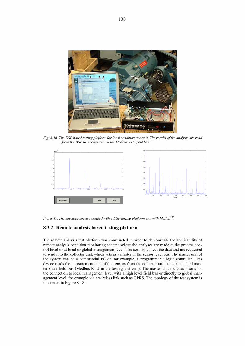
130

Fig. 8-16. The DSP based testing platform for local condition analysis. The results of the analysis are read

from the DSP to a computer via the Modbus RTU field bus.

0 50 100 150 200 250 300 350 4000

0.5

1

1.5

2

2.5

3

3.5

4

x 1014

0 50 100 150 200 250 300 350 4000

0.01

0.02

0.03

0.04

0.05

0.06

0.07

0.08

f[Hz]

Fig. 8-17. The envelope spectra created with a DSP testing platform and with MatlabTM .

8.3.2 Remote analysis based testing platform

The remote analysis test platform was constructed in order to demonstrate the applicability of remote analysis condition monitoring schema where the analyses are made at the process con-trol level or at local or global management level. The sensors collect the data and are requested to send it to the collector unit, which acts as a master in the sensor level bus. The master unit of the system can be a commercial PC or, for example, a programmable logic controller. This device reads the measurement data of the sensors from the collector unit using a standard mas-ter-slave field bus (Modbus RTU in the testing platform). The master unit includes means for the connection to local management level with a high level field bus or directly to global man-agement level, for example via a wireless link such as GPRS. The topology of the test system is illustrated in Figure 8-18.

131

The communications between sensors and the collector unit could be implemented with either a multi-channel data acquisition or with a field bus based solution. The advantages of a multi-channel realisation include simple communications protocol while each transmission line has only one communicating pair (the collector unit and the sensor unit), the possibility to make the interface between the sensor and the transmission simple and the use of fixed sensor cables. The field bus based approach provides the possibility to form a chain of sensor units of desired length. Also, a device that replaces the collector unit and fetches the data directly from the sen-sor units can be attached to the bus. This device may be for example a laptop computer. Furthermore, the amount of required electronics on the collector unit board is smaller than in the case of multi-channel realisation, because only one receiver/transmitter is needed. One of the disadvantages of this approach is a decreased reliability; a thread loose in one spot cancels the connection between the collector unit and all the sensor units. An error can also be produced due to multiple devices attached to the bus trying to transmit simultaneously. This can, how-ever, be effectively prevented with a proper design of communications protocol.

SLAVE

SLAVE

SLAVE

MASTER

SLAVE

MASTER

MASTER(PC, PLC etc.)

Collector unit

Sensor unit

SLAVE

SLAVE

Higher level Communication bus(Profibus, TCP-IP etc.)

Field bus

Sensor bus

Fig. 8-18. The topology of the remote analysis test platform with multiple collector units and sensors. All

communication is digital.

Collector unit. The main components of the collector unit are data memory (for storing the data collected from the sensor units), two communication ports for collector master communications and for sensor communications, a power supply and a microprocessor (Microchip's PIC18F8720) for the control of operations and communications. The schematic diagram and a prototype circuit board are presented in Figure 8-19.

132

MICROCON-TROLLERUNIT

DATA MEMORY (RAM)

EXTERNALCOMMUNICA-TIONS

COMMUNICA-TIONS WITH THE SENSOR UNITS

POWER SUPPLY

Address latches SRAM memory

PIC18microcontroller

Linearvoltageregulator

External bus connector

Sensor bus connector

Crystal oscillator

RS-485transceiver RS-485

transceiver

Switch

Power connector

Fig. 8-19. Block diagram of the collector unit

The AD converter of the sensor unit acquires 12-bit samples from the accelerometer at the sam-pling frequency of 20 kHz. The analysis described in Chapter 8.1.3 and illustrated in figures 8-5a and 8-5b requires about 30 000 samples. Thus at least 30 kilowords of 12 bits wide data memory is required. This equals to 45 kilobytes, if the samples are kept at 12-bit, and 60 kilo-bytes, if the samples are padded to 16 bits. This is far more than the data memory capacity of the PIC18F8720 and therefore, an external data memory is required. As previously noted, the samples transmitted by the sensor unit are 16 bits wide. Thus it is feasible to use data memory with the same word width. The AS7C1026 SRAM chip by Allied Semiconductor was used as external memory. Its word width is the required 16 bits and its capacity is 64 kilowords (128 kilobytes).

In an industrial environment, where the system is designed to be located, a 24 Volt DC supply is often available, but all the chips both in the collector unit and the sensor units require a regu-lated 5 V supply. The simplest solution to accomplish this is to provide both the collector unit and the sensor units with 24 V, which would can be regulated locally (on board) to the required 5 V using linear regulators. This would lead on to high power dissipation in the linear regulators due to a large voltage drop. In the case of the collector unit this should not be unsolvable prob-lem since there is plenty of space and thus cooling can be arranged, but the sensor units, enclosed in small tubes, might overheat. Another possibility is to regulate the 24 V input at the collector unit to 5 V and supply the sensor units with it. This realisation gains space savings on the sensor unit boards, since the regulator circuitry could have been left out. The selected reali-sation was a compromise of the two options described above. The 24 V supply is regulated to about 7 V at the collector unit using a switched type regulator. The collector units are then pro-vided with this voltage, which is regulated to 5 V locally on the sensor units using linear regulators.

Sensor. The sensor is based on a surface micromachined accelerometer tested in Chapter 7. The main components of the sensor unit are a micromachined accelerometer, an AD converter and a micro controller. Block diagram and a prototype circuit board of the sensor are presented in Figure 8-20.

133

ACCELEROMETERANALOGUE-TO-DIGITALCONVERTER

MICRO-CONTROLLER BUS DRIVER

PROGRAMMINGCONNECTION

CLOCKCIRCUIT

POWER SUPPLY

Fig. 8-20. Block diagram and a prototype circuit board of the sensor.

The analogue measurement data of the accelerometer was digitised with a 12-bit AD converter. The AD converter was interfaced to a micro controller with a standard SPI port. The micro controller does not possess external memory. Thus measurement data has to be transmitted real-time via a field bus to the collector unit.

The communication at the sensor level uses a master-slave type purpose-built field bus. It is implemented using the differential RS485 bus connection with the transmission rate 2.5 Mbps. The field bus cable is a two pair twisted cable, which includes the power supply, ground and differential signal wires.

8.3.3 Management level connection

The collected measurement data, in the remote analysis systems, must be analysed at the proc-ess control level or at the management level. Even when the local analysis is implemented the results of the analyses must be available at the management level. The outsourcing of service and maintenance is a growing trend. Therefore, the expert systems outside the plant require communications between the sensor level and the global management level. The communica-tions requirements depends much on the condition monitoring schema but also on the type of the plant where the system is implemented. The big industrial plants usually implement the industrial communication infrastructure of Figure 1-2. Many small plants are not connected to data communication buses but have a telephone line and are under coverage of cellular net-works. Therefore, the cellular connection between the local master unit of Figure 8-15 can be connected to a database of an outside plant with, for example, a dial-up Internet connection (Lindh, 2002e), (Ahola, 2003). In the big plants a global connection can be used also using the databases and information systems of a local management level (Lindh, 2001). On the other hand a system like that will require the data transfer from field-devices to the management level and data management actions at the local management level. For this reason, Ahola (2003) has suggested that a probable solution for the remote maintenance and diagnostics is the complete separation of the condition monitoring system from the information system of an industrial plant using the schema where the Internet connection is formed directly at the field level to an outside plant expert system as illustrated in Figure 8-21. This does not prevent local analysis, because the data can be achieved from the data bases at the global management level expert system via Internet connection and for example with JAVA (jdbc) techniques (Lindh, 2001).

Micromachinedaccelerometer

PIC16microcontroller

RS-485transceiver

Voltageregulators

134

Also the field level condition monitoring system can offer the data to the process control level with the communication path parallel to the Internet connection.

SensorReceiver Radio data transfer

Power-line data transfer

Twisted pair

data transfer

Fieldlevel

Process

INTERNET

- GSM ( GPRS, GSM Modem)- Telephone line (ADSL, ISDN)- Ethernet

REMOTE DIAGNOSTICS

Database:- Device registry- Measurement data- Service data

Software:- Fault analysis- Statistics

Processcontrol level

Managementlevel

Information system of industrial plant

Sensor

SensorSensorSensor

Fig. 8-21. Possible solution for outsourced diagnostics of an industrial plant. Condition monitoring sen-

sors are installed on the monitored devices. The sensor level data transfer is performed using various methods, such as power-line and radio communications. The Internet access required by the remote diagnostics is provided e.g. by using a wired or wireless telephone network. There is Internet access directly to the field level of the industrial plant. (Ahola, 2003)

8.3.4 Conclusions concerning embedded and remote analysis

The remote analysis schema has many advantages over the embedded schema. The investment costs of the system are probably smaller when the most calculations are made at management level where the calculation capacity is cheap and the data of several sensors can be calculated in any computer. The sensors can be constructed with low cost components (micro controllers), which operate at a wide temperature range. Also the power dissipation is minor compared to the dissipation of the high calculation capacity chips (e.g. DSP:s). Therefore, the temperature inside the sensor itself is not remarkably higher than the ambient temperature. The update of the analysis programs is possible and many different analyses can be done to one measurement data. Outside plant expertise can be utilised and the outsourcing of condition monitoring analy-sis work is possible at management level.

On the other hand the remote schema is totally dependent on the communications between the sensor and the analysing computer (no indication of a fault is possible without this). The em-bedded analyser does not necessarily require any external communications or analysis programs if automatic fault classification is included in the sensor. However, the communications buses may be required because there is often no local surveillance at the installation site.

135

8.4 Conclusions concerning the automatic analysis of the acceleration sig-nal

In this chapter, different methods for the creation of feature extractors that can be used for the bearing fault classification were compared. The classification possibilities were also compared. Two different pilot implementations and approaches to the integration of sensor, analyses and communications were presented.

Different feature extractors were tested. The efficiency of the feature extraction using an enve-lope spectrum method, an envelope autocorrelation method and an autocorrelation of joint time-frequency components were compared. Also, the envelope detection using Gabor- filter (STFT), digital pass band demodulation and Hilbert transform approach were compared. The best sepa-ration between the healthy and the broken cases was obtained using the envelope autocorrelation method or envelope spectrum method. The envelope detection can be carried out based on band pass demodulation technique or the Hilbert transform technique. The Hilbert-transformer demodulation suggests no a-priori-knowledge of the useful frame resonance fre-quency band. However, the use of a wide (1-8kHz) band does not remarkably attenuate the envelope spectrum components. Therefore both demodulation techniques are suitable for enve-lope detection.

The guidelines for statistical fault classification using the Mahalanobis distance and the deter-ministic classification with multi valued fuzzy logic and a combination of these were presented. Based on the tests, the automatic classification using the envelope spectra of frame vibration is possible. In the tests all tested signals were classified correctly, but the test data was rather limited. Therefore, one can not jump into conclusion that classification is possible in most cases before the tests are done with many motors with different bearing faults. Fuzzy logic analysing the envelope spectrum peak amplitudes can classify signals. However, by taking into account the qualitative features of the spectrum the discrimination power of the classification can be improved. In the tests, the statistical Mahalanobis distance based classifier was used as a pre-processor in conjunction with fuzzy logic.

The remote analysis schema where the sensors only collect the data and all analyses are made at the higher level in industrial communications and information infrastructure has many advan-tages over the embedded schema where the sensors analyse the measurement signal. The investment costs of the system are smaller when most of the calculations are made at manage-ment level where the calculation capacity is cheap and the data of several sensors can be calculated in any computer. The change of analysis programs is independent of sensors and the use of outside plant expert systems and organisations is more straightforward than in the em-bedded analysis schema.

136

9. SUMMARY AND CONCLUSIONS

In this chapter, the main results of this thesis are summarised. The main objective of this thesis was to evaluate methods that can be used in embedded condition analyses of the bearings of induction motors. The stator current measurement would be sufficient as the only condition monitoring sensor if bearing damages were detected with the stator current measurement based analyses. The feasibility of the stator current based methods in practical condition monitoring in an industrial motor drive was evaluated with a 15 kW induction motor. The methods were con-cluded not to be reliable enough the practical use. For this reason, vibration monitoring is required for the detection of bearing faults. The vibration monitoring devices must be fixed to a motor frame. Economical means for constructing vibration monitoring as a part of a condition monitoring concept was surveyed.

9.1 Key results of the thesis

Main contribution 1: The mathematical model of a cyclic bearing fault was further developed with the presentation of a model that explains the features found in a measured acceleration signal. The model separates the origins of vibration into non-modulating and modulating effects and handles the motor frame as a linear system. With the proposed model, the simulation results and measurements correspond in joint time- frequency domain. The phenomena of stator cur-rent transient due to radial movement of the rotor were theoretically estimated. It was estimated that the current transient should appear but that the amplitude of the transient is very small, from a few milliamperes up to tens of milliamperes.

Main contribution 2: The effects of the radial shocks to rotor of the induction machine were experimentally tested with a DC magnetised motor. This allowed for modulation effects to be avoided and a reliable view of an actual stator transient current signal could be isolated. The theoretically evaluated estimate of magnitude of the transient could be ensured.

Main contribution 3: The verification of the feasibility of the stator current measurement as a bearing fault indicator was experimentally tested with a running 15 kW induction motor. The spectrum of the stator current signal was analysed. A Mahalanobis distance calculation based classification of the stator current signal was analysed with simulation and experimental results using actual measurements.

Simulation was used to show that the classification based on the Mahalanobis distance is possi-ble if radial movement at the bearing pass frequency is present but that the noise in the measurement chain and the non-sinusoidal time varying air gap flux can prevent the indication of a fault.

The outer race defect was clearly indicated only in the case of the large internal radial clearance of the bearing (internal radial clearance class C4 bearings). Normal wear (=large clearance) could not be distinguished from the bearing damage. This was tested using the bearings of dif-ferent internal radial clearance classes in calculations.

The large internal radial clearance allows large radial movement of the rotor. On the other hand, the radial movement of the rotor is affected by the magnetic pull between the rotor and the stator. In the ideal situation the value of this pull is zero. The magnetic pull is increased with the degree of the rotor eccentricity. The free eccentricity is increased if the radial clearance of bear-

137

ing is great. This free eccentricity can rotate parallel to the maximum of the air gap flux density causing the biggest possible force in the direction of the flux maximum causing the biggest change in the stator current. In addition, load eccentricity can affect the size and the direction of the radial movement of the rotor.

In many researches the stator current signal has been found feasible in bearing fault monitoring. In this research, it was found that the internal radial clearance has significant influence on the classification possibilities. This result may also explain the different conclusion. In most ex-periments, a tested motor was relatively small. For example in the experiment of reference (Yazici, 1999) a ¾ HP induction motor was tested. In such a small induction motor, the ratio between the internal radial clearance of bearing and air gap length is greater than in the case of the bigger motor. Also, the smaller diameter of the rolling element of the bearing allows greater movement of the rotor for the same size of the hole in the bearing race. These factors may lead to a bigger stator current transient.

The main conclusion is that the stator current measurement as a bearing fault indicator is not adequate in the case of the 15 kW 4-pole motor with a bearing with a normal radial clearance. Therefore a feasibility of the stator current measurement as a bearing fault indicator is ques-tionable in practical condition monitoring where high reliability of analysis is required.

Main contribution 4: The micromachined accelerometers are one alternative to traditional piezo-electric sensors. The characteristics of traditional piezoelectric sensors and capacitive micromachined sensors were presented and the effects of the features and performance limita-tions on condition monitoring of bearings of electric motors were discussed. The performances of the micromachined chip and piezoelectric sensors were compared when the envelope spec-trum method was used in analyses.

The envelope spectrum method can be used with a micromachined sensor and relatively small faults can be diagnosed. The detection of the most incipient faults (frame response <10mg) that can be found using the piezoelectric sensor is not possible due to the bigger noise level of the micromachined accelerometer. On the other hand, if the dominant vibration is big (crushers, cavitating pumps, piston compressors etc.) the amplitude range of the micromachined acceler-ometer is not adequate. However, the measurement range given in the manufacturer datasheet can be exceeded because the amplitude of the peaks has little effect on the bearing defect analy-sis based on an envelope spectrum.

Main contribution 5: The outsourced service and condition monitoring is a growing trend in the industry. This trend sets new requirements for condition monitoring. The outside plant organisa-tions must have means to access the information systems of an industrial plant. On the other hand, the profitability of automatic analysis tools increases. In this thesis guidelines for the automatic detection of bearing faults were given and a condition monitoring schema based on an embedded, sensor analysis as well as a schema based on the remote analysis were discussed. The remote schema means a system where sensors collect the measurement data but the analy-ses are made at a higher level in the industrial information infrastructure.

The automatic fault analysis consists of the feature extraction and the fault classification. Dif-ferent feature extraction methods were tested. These methods include the autocorrelation, Gabor-filter based method, the digital pass band demodulation and the Hilbert transformer ap-proaches. The methods were used for the envelope detection of an acceleration signal. Therefore, the methods were compared in conjunction with the envelope spectrum method and their ability to separate features in the envelope spectra was mainly used as a measure of the performance. The Hilbert transformer approach and the band pass demodulation method were

138

evaluated as the best solution because of their ability to extract features and their computational efficiency which is an important issue especially in the case of an embedded analysis schema. If the condition analysis is not made at the field level, the computational efficiency is not so im-portant. Then, the autocorrelation envelope method can be preferable, since based on the tests it seems to be equal or better than the Hilbert transformer approach or the band pass demodulation method as a feature extractor. The selections were based on the visual inspection of the enve-lope spectra.

The guidelines for the statistical fault classification using the Mahalanobis distance and deter-ministic classification with multi valued fuzzy logic and a combination of these were presented. Based on the tests, automatic classification using the envelope spectra of the frame vibration is possible using either approach.

The method where the Mahalanobis distance based statistical classification results were used as an one input in fuzzy logic was introduced. This input and other qualitative features of the spec-trum were taken into account in the fuzzy logic which evaluated the probability of a certain fault. The other fuzzy logic evaluated the degree of certain fault and by combining the outputs of these logics, the final suggestion of the state and required action were given. Based on the tests, this approach improves the reliability of the fault analysis when the reliability of the analysis means the minimization of the wrong action, continuing the use or repairing the motor. In many researches the neural network has been used as a pre- processor for the fuzzy logic. The presented approach is alternative to that approach. The statistical Mahalanobis distance based classifier as used in this thesis may give equal results to the neural network. However, due to the exact input output relationship, the controllability of the classification is better when the Mahalanobis distance classifier is used.

The test data was rather limited and jumping to certain conclusions should not be made before the tests are done with many motors with different bearing faults. On the other hand, by discuss-ing the possibilities of an automatic fault analysis, the guidelines for the future work are given.

The remote analysis schema where the sensors only collect the data and all analyses are made at the higher level in industrial communications and information infrastructure have many advan-tages over the embedded schema where the sensors analyse the measurement signal. The investment costs of the system are smaller when the most calculations are made at management level where the calculation capacity is cheap and the data of several sensors can be calculated in any computer. The change of analysis programs is independent of the sensors and the use of outside plant expert systems, and organisations is more straightforward than in the embedded analysis schema.

9.2 Conclusions

The predictive condition monitoring of electrical motors means continuous or periodical evalua-tion of the healthiness of the motor. The main objective of the condition monitoring is to alarm againt future damage if no action is taken. On the other hand, if service and condition monitor-ing is a business for an outside plant organisations, the importance of the effectiveness of the condition monitoring increases. The organisation that performs the service actions must be able to guarantee and ensure the continuous use of the devices that they are responsible for and fail-ing in this goal may have a much bigger importance on this organisation than the organisation that uses the devices for the production since monitoring is its core business area. In addition to that the organisation that does the condition monitoring with the minimum costs is in a favour-able market situation. When the labour costs are remarkable in condition monitoring the

139

minimisation of labour is one of the most important factors that effects the effectiveness of the condition monitoring. Therefore, the means that make it possible to utilise the monitoring and analyses automatically have become important. At the same time, the industrial and other in-formation systems have enabled the remote data collection and monitoring.

In this thesis, tests were done in order to clarify the possibilities to construct an automatic on-line condition monitoring system for the electric motors. It proposes that for the bearing fault detection, the vibration measurement is required. On the other hand, the rotor fault detection, for example, is not reliable using the vibration measurement only. Therefore, more than one measurement is required if all of the principal failure types of an induction motor are to be cov-ered.

The automatic bearing fault analysis (cyclic faults), based on the results of the tests, is possible. Yet, much research work must be done before such a system is reliable enough for the practical use.

The results of this research can be applied in research and development. The thesis gives guide-lines for future research in the area of automatic fault analysis and proposes the condition monitoring schemas that hopefully may give ideas for developers of condition monitoring de-vices and systems.

140

References

(ABB, 1999) ABB Motors, The motor guide, 1st edition, ABB Automation power products, LV Motors, Vaasa, 1999, ISBN 952-91-0728-5

(Ahola, 2000) Jero Ahola, Tuomo Lindh, Jarmo Partanen, Pertti Järventausta and Markku Kauppinen, “Data Management System for DMS in Industrial Environment”, Distributech DA/DSM Europe 2000, Austria 10-12 October 2000.

(Ahola, 2003) Jero Ahola, Applicability of power-line communications to data transfer of on-line condition monitoring of electrical drives. Dissertation, Acta Universitatis Lappeenrantaensis 157, Lap-peenranta University of Technology, Finland 2003, ISBN 951-764-772-7.

(Albrecht, 1986) Albrecht, P.F., McCoy, R.M., Owen, E.L., “Assesment of the reliability of motors in utility applications”. IEEE transactions on energy conversion, Vol. EC-1, No.1, March 1986.

(Arkkio, 1996) Arkkio A., “Unbalanced magnetic pull in cage induction mo-tors- dynamic and static eccentricity”, 1996, Proceedings of ICEM ’96, Vigo, Spain,Vol. 1, pp. 192-197.

(Baillie, 1996) Baillie D. C., Mathew J., “A comparison of autoregressive modeling techniques for fault diagnosis of rolling element bear-ings” Mechanical systems and signal processing, 1996, No.10, pp. 1-17

(Benbouzid, 2001) Benbouzid, M.E.H., Nejjari, H., “A simple fuzzy logic ap-proach for induction motors stator condition monitoring”, IEMDC 2001, Electric Machines and Drives Conference, 2001, pp. 634 –639.

(Bernstein, 1999) J. Bernstein, R. Miller, W. Kelley, P. Ward, “Low-Noise MEMS Vibration Sensor for Geophysical Applications”, Jour-nal of microelectromechanical systems, Vol. 8, No. 4, December 1999.

(Blaschke, 1996) Blaschke, F., van der Burgt, J., Vandenput, A., “Sensorless direct field orientation at zero flux frequency”, Industry Appli-cations Conference, 1996. Thirty-First IAS Annual Meeting, IAS '96., Conference Record of the 1996 IEEE Volume: 1 , 1996 , Page(s): 189 -196 vol. 1.

(Bonato, 1997) Bonato B., Ceravolo R., De Stefano A., Knaflitz M., “Bilinear time-frequency transformations in the analysis of damaged structures”, Mechanical systems and signal processing, 1997, No.4, pp. 509-527

(Bonnett, 1992a) Bonnett, A.H., Soukup G.C., “Cause and analysis of stator and

141

rotor failures in three-phase squirrel-cage induction motor”, IEEE Industry Applications, Vol 28. , Issue 4, July/August 1992, pp. 921-937.

(Bonnett, 1992b) Bonnett, A.H., “Cause and analysis of bearing failures in elec-trical motors”, Petroleum and Chemical Industry Conference, 1992, Record of Conference Papers, Industry Applications So-ciety 39th Annual , 28-30 Sep 1992 , pp. 87 –95.

(Busse, 1997) Busse, D., Erdman, J., Kerkman, R., Schleger, D., Skibinski, G., “Characteristics of shaft voltage and bearing currents”, IEEE Industry Applications, Vol. 3. , Issue 6, November/December 1997, pp. 21-32

(Chow, 1984) Chow M. Magnum M., Sui O. Y., “A neural network approach to real-time condition monitoring of induction motors”, IEEE transactions on industrial electronics, Vol. 38. , No.6, Decem-ber 1991, pp. 448-453.

(Cohen, 1995) Cohen Leon, Time-frequency analysis. Prentice-Hall, Inc., USA, 1995. ISBN 0-13-594532-1.

(Cover, 1991) Cover, T.M., Thomas, J.A., Elements of Information Theory. John Wiley and Sons, 1991.

(Crenna, 1996) Crenna, F., Michelini, R.C., Rossi, G.B., “Measuring vibration patterns for rotor diagnostics”. Instrumentation and Measure-ment Technology Conference, IMTC-96. Conference Proceeedings. 1996, pp. 597 –602.

(Daubechies, 1990) Daubechies, I., "The wavelet transform, time-frequency local-ization and signal analysis", IEEE transactions on information theory, Vol. 36, No. 5. September 1990, pp. 961-1005.

(Dorrell, 1995) Dorrell, D.G., Thomson, W.T., Roach, S., ”Combined effects of static and dynamic eccentricity on airgap flux waves and the application of current monitoring to detect dynamic eccentricity in 3-phase induction motors.”, Seventh International Confer-ence on Electrical Machines and Drives. 1995, pp. 151 -155.

(Dorrell, 1997) Dorrell, D.G., Thomson, W.T., Roach, S., ”Analysis of airgap flux, current, and vibration signals as a function of the combina-tion of static and dynamic airgap eccentricity in 3-phase induction motors.”, IEEE transactions on industry applications. Vol. 33, No. 1, January/February 1997, pp. 24 -34.

(Duda, 2000) Richard O. Duda, David G. Stork, Peter E. Hart. Pattern Classi-fication, 2000, John Wiley & Sons Inc; ISBN: 0471056693

(Dorrell, 1999) Dorrell, D.G., ”Experimental behavior of unbalanced magnetic pull in 3-phase induction motors with eccentric rotors and the relationship with tooth saturation”, IEEE transactions on energy conversion, Vol. 14, No. 3, September 1999, pp. 304 -309.

142

(Ellison, 1997) Ellison, A. J., Yang, S. J., ”Effects of rotor eccentricity on ac-coustic noise from induction machines”, Proceedings IEE, 118(1), pp. 174-183. January 1997.

(Engel, 1979) Engel, L., Winter, H., Antriebstechnik 18, Vol 3. , June 1979, pp. 79-74. In German.

(Eren, 2001) Eren Levent, Devaney Michael J., "Motor Bearing Damage Detection Via Wavelet Analysis of the Starting Current Mo-ment", IEEE Instrumentation and Measurement Technology Conference, Hungary, Budabest, May 21-23.2001.

(FAG, 1997) FAG Bearings corporation, Rolling bearing damage, FAG South East Asia PTE Ltd., 1997, Publ. No. WL 82 102/2 Esi, 71

(Forrester, 1989) Forrester P.D., “Use of the Wigner Ville distribution in helicop-ter transmission fault detection”, Proceedings of the Australian Symposium on Signal Processing and Applications ASSPA A 89, 1989.

(Ishida, 1984) Ishida M., Iwata K. “A new slip frequency detector of an induc-tion motor utilizing rotor slot harmonics,” IEEE transactions on industry applications, 1984, Vol. IA-20. , No.3, pp. 575-581

(Islam, 1996) Islam,H. M., Mostafa, M.G., “Novel microprocessor based negative phase current relay and meter”, 1996, Electrical power & energy systems. Vol. 18. No 8, pp.547-552.

(Kämaräinen, 2002) Joni-Kristian Kämäräinen, Ville Kyrki, Tuomo Lindh, Signal Discrimination Based on Power Spectrum of Filter Response, Tutkimusraportti 80 (TITE), Lappeenranta University of Tech-nology, Lappeenranta, ISBN 951-764-683-6, 2002

(Kang, 2002) Kang M. S., Stanbridge A. B., Chang T. G., Kim H. S., “Meas-uring mode shapes with a continuously scanning vibrometer- Hilbert transform approach”. Mechanical systems and signal processing, 2002, No.16 (2-3), pp. 201-210

(Karasaridis, 1997) Karasaridis, A., Maalej, M., Pantazopoulou, S., Hatzinakos, D., ” Time-frequency analysis of sensor data for detection of struc-tural damage in instrumented structures”, DSP 97., 13th International Conference on Digital Signal Processing, Confer-ence Proceeedings. 1997, pp. 817-820.

(Kim , 1994) Kim Y. R., Sul S. K.,Park M. H. “Speed sensorless vector con-trol of induction motor using extended Kalman filter,” IEEE transactions on industry applications, 1994, No.3, pp. 1225 –1233.

(Kliman, 1998) Kliman Gerald B., Premerlani William J., Yazigi Birsen, Koegl Rudolph A. “Recent development in on-line motor diagnostics”, ICEM 98 conference proceedings, Istanbul, 1998, pp. 471-475.

143

(Kokko, 2003) Kokko Voitto, Condition monitoring of squirrel-cage motors by axial magnetic flux measurements, Acta Universitatis Ouluensis C 179, Oulu, 2003, 151 s. ISBN 951-42-6937-3,

(Kovács, 1959) Kovács K.P., Rácz I., Transiente Vorgänge in Wechselstrom-maschinen. Verlag der Ungarischen Akademie der Wissenschaften, Budapest, 1959. 514p.

(Krzanowski, 1979) Krzanowski W. J. Principles of Multivariate Analysis, Aca-demic press, London, 1979.

(Kubota , 1994) Kubota H., Matsuse K. “Speed sensorless field-oriented control of induction motor with rotor resistance adaptation,” IEEE transactions on industry applications, 1994, Volume: 30 5 , Sept.-Oct. Page(s): 1219 -1224

(Kyusung, 2002) Kyusung, K., Parlos A. G., ”Induction motor fault diagnosis based on neuropredictors and Wavelet signal processing”, IEEE transactions on mechatronics, Vol. 7, No.2, June 2002.

(Lachenbruch, 1975) Lachenbruch, P.A., Discriminant analysis, Hafner: New York, 1975.

(Lempiäinen, 1995) Lempiäinen Tommi, Yhteenveto Kaukopään kunnossapidolli-sista häiriöistä ja kunnossapidon toteutuksesta, Insinöörityö, 1995. In Finnish.

(Lindh, 2001) Tuomo Lindh, Jero Ahola, Jarmo Partanen, Sauli Antila, Pertti Järventausta, Kimmo Kivikko, Pekka Verho, Pekka Ruupunen. ”Web-based monitoring functions utilising data management system”, DistribuTECH Europe 2001, Berlin 6-8 November 2001

(Lindh, 2002a) Tuomo Lindh, Jero Ahola, Jarmo Partanen, Bearing monitoring of electrical motors and powerline communications in low volt-age industrial distribution networks, Tutkimusraportti/ Research report 16, TESLA- raportti 79/2002.

(Lindh, 2002b) Tuomo Lindh, Jero Ahola, Jarmo Partanen, ”An Evaluation of Condition Monitoring of Bearings of 15 kW Induction Motor Based on Stator Current Measurement”, ICEM 2002 conference proceedings, Bruges, Belgium 26-28 August, 2002.

(Lindh, 2002c) Tuomo Lindh, Jero ahola, Jarmo Partanen, ”An Evaluation of micromachined accelerometer in the Condition Monitoring of Induction Motor Bearings”,VANEM 2002 3rd International Seminar on Vibrations and Acostic Noise of Electric Machin-ery, Lodz, Poland, 17-19 October 2002.

(Lindh, 2002d) Tuomo Lindh, Jero ahola, Jarmo Partanen, ”Effects of Internal Radial Clearance of Bearings to Condition Monitoring of Bear-ings of Induction Motor Based on Statistical Stator Current Analysis”, VANEM 2002 3rd International Seminar on Vibra-

144

tions and Acostic Noise of Electric Machinery, Lodz, Poland, 17-19 October 2002.

(Lindh, 2002e) Tuomo Lindh, Jero Ahola, Jarmo Partanen, ”Communication Possibilities for Remote Control and Condition Monitoring of Small Scale Power Plant”, NORDAC 2002, Copenhagen, Den-mark, 7-8 November, 2002.

(Lindh, 2003) Tuomo Lindh, Jero Ahola, Joni- Kristian Kämäräinen, Ville Kyrki, Jarmo Partanen, “Bearing Damage Detection Based on Statistical Discrimination of Stator Current”, SDEMPED 4th IEEE International Symposium on Diagnostics for Electric Ma-chines, Power Electronics and Drives, August, 2003, Atlanta, Georgia, USA, pp. 177-181

(Mahalanobis, 1936) P. C. Mahalanobis, Proc. Natl. Institute of Science of India, 2, 49, 1936.

(Mardia, 1971) Mardia K. V., "The effect of non-normality on some multivari-ate tests and robustness to non-normality in the linear model", Biometrica, Vol. 58, Issue 1, April 1971.

(Mechefske, 1998) Mechefske C. K., “Objective machinery fault diagnosis using fuzzy logic”. Mechanical systems and signal processing, 1998, No.12, pp. 855-862

(Mohd-Yasin, 2001) Mohd-Yasin, F., Korman C.E., Nagel D.J., “Measurement of noise characteristics of MEMS accelerometers”, Semiconductor Device Research Symposium, 2001 Interna-tional, 5-7 December, 2001, p.p. 190 –193.

(Nikolaou, 2002) Nikolaou N. G., Antoniadis I. A., “Demodulation of vibration signals generated by defects in rolling element bearings using complex shifted Morlet wavelets”. Mechanical systems and sig-nal processing, 2002, No.16 (4), pp. 677-694

(Ocak, 2001) Ocak Hasan, Loparo Kenneth A., “A new bearing fault detec-tion and diagnostics schema based on hidden Markov modeling of vibration signal”, IEEE International Conference on Acous-tics, Speech, and Signal Processing, 2001. Proceedings., Vol.5, 2001. pp. 3141 –3144.

(Pan, 1996) Pan M.C., Sas P.,Van Brussel H., “Nonstationary Time-Frequency Analysis for Machine Condition Monitoring”, Pro-ceedings of the IEEE-SP International Symposium on Signal Processing, 1996, Pp. 477- 480.

(Partanen, 1999) Jarmo Partanen, Tuomo Lindh, Pertti Järventausta, Markku Kauppinen, Pekka Verho, Matti Kärenlampi, ”Intelligent appli-cations for the management of electrical systems in industrial plants”. Proceedings of ISAP'99 (Intelligent System Application to Power Systems), Rio de Janeiro, Brazil, April 1999

145

(Paya, 1997) Paya P. A., Esat I. I. “Artificial neural network based fault di-agnostics of rotating machinery using Wavelet-transforms as a preprocessor”, Mechanical systems and signal processing, 1997, No.11, pp. 751-765

(Penman, 1994) Penman J., Yin C.M. “Feasibility of using unsupervised learn-ing, artificial neural networks for the condition monitoring of electrical machines”, IEE proceedings on electric power appli-cations, vol 141, No.6, pp. 317-322, November 1994.

(Penny, 1996) Penny, K., I., "Appropriate critical values when testing for a single multivariate outlier by using the Mahalanobis distance", Applied Statistics, Vol. 45, No.1, November 1996.

(Proakis, 1996) John Proakis, Dimitris Manokolakis, Digital Signal Processing, Prentice- Hall, New Jersey, USA, 1996

(Rajashekara, 1996) K. Rajashekara, A. Kawamura, K. Matsuse, “Sensorless control of AC motor drives,” IEEE Press 1996, New York, ISBN 0-7803-1046-2

(Rao, 1996) Rao, B.K.N. Handbook of condition monitoring, 1st edition, Oxford, Elsevier Advanced Technology, 1996. ISBN 1-85617-234-1. pp.97-114.

(Riley, 1998) Riley C. M., Lin B., Habetler T. G., Schoen R. R., "A method for sensorless on-line vibration monitoring of induction ma-chines", IEEE transactions on industry applications, Vol. 34, No.6, November/December 1998.

(Salles, 2000) Salles G., Filippetti F., Tassoni C., Grellet G., Franceschini G., ”Monitoring of Induction Motor Load by Neural Network Techniques”, IEEE transactions on power electronics, Vol. 15, No.4, July 2000.

(Schiltz, 1990) Schiltz, R. L., “Forcing frequency identification of rolling ele-ment bearings”, Sound and vibration, pp. 16-19, May 1990.

(Schoen, 1994) Schoen, R.R., Lin, B.K., Habetler, T.G., Schlag, J.H., Farag, S., “An unsupervised, on-line system for induction motor fault detection using stator current monitoring”, Industry Applica-tions Society Annual Meeting, 1994, Conference Record of the 1994 IEEE, 2-6 Oct 1994 pp. 103 –109.

(Schoen, 1995) R.R. Schoen, T. Habetler, "Motor bearing damage detection using stator current monitoring", 1995 IEEE Industry applica-tion society annual meeting conference proceedings.

(Spatenka, 2002) Spatenka Petr, Methods of design and testing of real time sys-tems, Master’s thesis, Lappeenranta University of Technology, Lappeenranta, 2002.

(Spatenka, 2003) Spatenka Petr, Lindh Tuomo, Jero Ahola, Jarmo Partanen. Em-

146

bedded DSP based system for bearing condition monitoring of electric motors, Tutkimusraportti/Research Report 17, Lappeen-ranta University of Technology, Lappeenranta, 2003, ISBN 951-764-822-7.

(Staszewski, 1997) Staszewski W. J., Worden K., Tomlison G. R., “Time-Frequency Analysis in Gearbox Fault Detection Using the Wigner-Ville Distribution and Pattern Recognition”, Mechani-cal systems and signal processing, 1997, No.11, pp. 673-692

(Tavner, 1987) Tavner, Peter J., Penman James, Condition monitoring of elec-tric motors, 1st edition, Research studies press Ltd, England, 1987. ISBN 0-86380-061-0.

(Tímár, 1989) Tímár, P. L., Fazekas, A., Kiss, J., Miklós, A., Yang, S. J., Noise and vibration of electrical machines, Studies in electrical and electronic engineering 34, Elsevier, Amsterdam, 1989.

(Vas, 1993) P. Vas, Parameter estimation, condition monitoring, and diag-nosis of electrical machines, Oxford University Press Inc., 1993, ISBN 0-19-859375-9

(Wang, 1998) Wang Y. F., Kootsookos P. J., “Modelling of Low Shaft Speed Bearing Faults for Condition Monitoring”. Mechanical systems and signal processing, 1998, No.12, pp. 415-426

(Wang, 1996) Wang Y. F., Harrap M. J., “Condition monitoring of ball bear-ings using envelope autocorrelation technique”. Machine Vibration, 1996, No.5, pp. 34-44

(Wilks, 1963) Wilks, S. S. "Multivariate statistical outliers", Sankhya A, 25, 1963. pp 407 –426.

(Yazici, 1999) Yazici B., Kliman G. B., ”An Adaptive Statistical Time-Frequency Method for Detection of Broken Bars and Bearing Faults in Motors Using Stator Current”, IEEE transactions on industry applications, Vol. 35, No.2, March/April 1999.

(Yen, 2000) Yen, G., G., Lin, K.,, ”Wavelet packet feature extraction for vibration monitoring”, IEEE transactions on industrial elec-tronics, Vol. 47, No.3, June 2000.

(Yin, 1995) Yin Randy R., Schoen et. Al., "Motor bearing damage detection using stator current monitoring", IEEE transactions on industry applications, Vol. 31, No.6, November/December 1995.