ON THE COMPUTATION OF A PRECISE GEOID TO QUASIGEOID …

ON THE COMPUTATION OF

A PRECISE GEOID – TO – QUASIGEOID SEPARATION

S. Hejrati a,*, M. Najafi-Alamdari b

a Dept. of Engineering, Azad University, Science and Research Branch, Shahrood, Iran – [email protected] b Dept. of Engineering, Azad University, North Tehran Branch, Tehran, Iran – [email protected]

KEY WORDS: Orthometric height, Normal height, Geoid, Quasigeoid

ABSTRACT:

In geodesy, orthometric and normal heights are considered as basic height systems on the earth. The reference surfaces for these heights

are the geoid and quasigeoid respectively. Taking advantage of GNSS measurements, one can achieve a precise solution for the geoid

and for the quasigeoid. Two methods, called direct and indirect, are worked out in this research for the computation of separation

between geoid and quasigeoid in a mountainous region in the USA. The area selected for this purpose is mountainous and rough enough

in order to be able to show the effect of roughness of topography in the sought quantity. The results of the two methods and testing

them against GNSS-Levelling on 445 known points indicates an accuracy of 1.3 cm in RMS scale with the direct method, where there

is 7 cm as an average difference between the observed geoid and quasigeoid separation and the same quantity derived from the direct

method. Using Chi-squared goodness of fit test showed that the distribution of the residual quantities are normally distributed in the

test area.

1. INTRODUCTION

Two concepts of Stokes-Helmert (Helmert, 1890) and

Molodensky (Molodensky et al. 1960) approaches are used to

solve geodetic boundary-value problem for geoid and

quasigeoid heights both referred to the normal ellipsoid. The

geoid and quasigeoid are in turn reference surfaces to measure

orthometric and normal heights on the earth respectively. The

separation between geoid and quasigeoid is usually needed, in

practice, for transformation of one system of height to another.

There is, however, an approximate formula in literature

(Heiskanen and Moritz, 1967) to compute

Geoid-to-Quasigeoid Separation (GQS) using Bouguer gravity

anomaly; and it is also based on the known orthometric height

at a point of interest. Precise estimation of Bouguer gravity

anomaly requires more detailed topographical height

information around the point.

So far, many studies have been conducted for the

determination of GQS. Sjoberg (1995) uses a model of

orthometric height of higher order precision in the

approximate formula (Heiskanen and Moritz, 1967) in order to

reduce the terrain effect uncertainties. Rapp (1997) used

precise height anomaly into the approximate formula.

Nahavandchi (2002) used the Rapp technique as an indirect

method for numerical evaluation on Iran's region

GNSS-Levelling data. Sjoberg (2006) offered a precise

formula, including terrain correction term and a term with

regard to lateral variation of topographical densities for

conversion from normal height to orthometric height. Tenzer

et al. (2006) estimated the GQS by a correction model based

on the mean gravity disturbance along the vertical within the

topographic masses. Flury and Rummel (2009) derived the

magnitude of the GQS equal to 24 and 48 cm in two test areas

of the Alps. Sjoberg (2010) presented a strict formula for the

GQS with two terms, terrain and gravimetric corrections. The

result of his study improved the accuracy of Flury and Rummel

formula up to 1 cm. Sjoberg (2012) used an arbitrary gravity

correction model to improve the rough topographic effects

accuracy on the GQS. Sjoberg and Bagherbandi (2012)

evaluated the magnitude of this separation using the EGM08

and DTM2006 models complete to harmonic degree and order

2160 in the Tibet plateau and Indian Ocean to 5.47 and 0.11

m, respectively. Bagherbandi and Tenzer (2013) estimated the

value of the GQS by GOCO02S model complete to degree 250

on the Tibet plateau and the Himalayan Mountains ranging

from 0.15 to 3.62 m. The comparison of their results with

EGM08 model shows ±20 cm differences. Sjoberg (2015)

presented a rigorous scheme to estimate GQS using gravity

disturbance expansion to Taylor series along plumbline. In his

study, he used three different correction methods, applying the

Bouguer gravity disturbance, an arbitrary compensation model

and analytical continuation technique.

In this study two methods called direct and indirect are

worked out to accurate estimation of GQS. Topographic

masses above the geoid are a major obstacle in the gravity field

determination. Hence, in two mentioned methods, different

models for topographic effects are used. Finally, to show the

precision superiority, in each one of two methods, the

The International Archives of the Photogrammetry, Remote Sensing and Spatial Information Sciences, Volume XLII-4/W4, 2017 Tehran's Joint ISPRS Conferences of GI Research, SMPR and EOEC 2017, 7–10 October 2017, Tehran, Iran

This contribution has been peer-reviewed. https://doi.org/10.5194/isprs-archives-XLII-4-W4-489-2017 | © Authors 2017. CC BY 4.0 License. 489

magnitude of geoidal height extracted from methods are

compared with geometric geoidal height obtained

GNSS-Levelling stations in test area.

2. DIRECT METHOD IN DETERMINATION OF

GEOID TO QUASIGEOID SEPARATION

The orthometric and normal heights H and 𝐻𝑁 of a point on

the earth are derived to be, (Heiskanen and Moritz, 1967),

𝐻 =𝐶

�̅� (1)

𝐻𝑁 =𝐶

�̅� (2)

where, C is the geopotential number, �̅� and �̅� are the mean

actual and mean normal gravities along the actual plumb line

from the geoid up to the point of interest and normal plumb

line from the normal reference ellipsoid up to the telluroid

respectively. The separation between the geoid and the

quasigeoid (GQS) as the difference between normal and

orthometric heights is given by, (ibid),

𝐻𝑁 −𝐻 = 𝑁 − 𝜁 =�̅�−�̅�

�̅�𝐻 (3)

where, Zetta, is the height anomaly and N is the geoidal height

at the computation point. The evaluation of �̅� alone in practice

is problematic since the information required about density

distribution inside the earth around the point of interest is less

reliable. The suggested solution is to approximate the

differential �̅� − �̅� term with the Bouguer gravity anomaly Δ𝑔𝑃𝐵

at a computation point P. Therefore, the estimation of GQS is

given by the formula (ibid).

𝑁 − 𝜁 ≈Δ𝑔𝑃

𝐵

�̅�𝐻 (4)

The formula above does not provide the required accuracy in

mountainous areas due to the uncertainty in terrain correction

(Helmert, 1890; Niethammer, 1932). Using Bruns formula, the

disturbing potential is converted to geoid height and/or to

height anomaly through normal gravity (Bruns, 1878;

Molodensky et al., 1960).

𝑁 =𝑇𝑔

𝛾0 and or⁄ 𝜁 =

𝑇𝑃

𝛾𝑄 (5)

where subscripts 𝑃 and 𝑔 denote locations on the Earth and

geoid surfaces respectively, 𝛾0 and 𝛾𝑄 represent the normal

gravities on the reference ellipsoid with geocentric radius 𝑟0

and on the telluroid surface with 𝑟𝑡 radius, respectively.

Radius 𝑟𝑡 equals the sum of 𝑟0 radius and normal height 𝐻𝑁.

In Eq. (5) we can represent the disturbing potential T in form

1 Analytical continuation bias

of spherical harmonic series as a (𝑟, Ω) point according to the

following expansion that is complete to M harmonic degree.

𝑇(𝑟, Ω) = ∑ (𝑅

𝑟)𝑛

𝑀𝑛=2 ∑ 𝑇𝑛𝑚

𝑛𝑚=−𝑛 𝑌𝑛𝑚(Ω) (6)

where 𝑌𝑛𝑚 and 𝑇𝑛𝑚 are fully normalized spherical harmonics

and spherical harmonics coefficients of disturbing potential of

degree 𝑛 and order 𝑚, respectively, 𝑀 is the maximum degree

of expansion, Ω = (𝜃, 𝜆) the spatial angle at point of spherical

coordinates co-latitude 𝜃 and longitude 𝜆. Considering Eq. (5),

the expression of a strict model for GQS with the terrain

correction term as following formula is given (Sjoberg, 2006).

𝑁 − 𝜁 =𝑇𝑔

𝛾0−

𝑇𝑃

𝛾𝑄+𝐴𝐶𝐵

𝛾0 (7)

where the ACB1 is the topographic bias. This bias is evaluated

applying external series expansion of earth gravity potential

inside the topography. The following formula estimates the

magnitude of the ACB to fourth powers of elevation according

to spherical approximation and a constant density for

topographic masses (Agren, 2004; Sjoberg, 2007).

𝐴𝐶𝐵 = −2𝜋𝜇 [𝐻2 +2

3

𝐻3

𝑅+𝑛(𝑛+1)

12

𝐻4

𝑅2] (8)

where 𝜇 = 𝐺𝜚, 𝐺 is gravitational constant, 𝜚 being the density

of crust and for topographic height powers with its coefficients

the following expansions exists

𝐻𝑛𝑚𝜈 =

1

4𝜋∬ 𝐻𝜈 𝑌𝑛𝑚 𝑑𝜎𝜎

for 𝜈 = 2,3,4 (9)

𝐻𝜈 = ∑ 𝐻𝑛𝑚𝜈

𝑛,𝑚 𝑌𝑛𝑚 (10)

In Eq. (7), by using downward continuation technique and

Taylor series, the following conversion between the telluroid

and reference ellipsoid surfaces is expressed for normal

gravity (Molodensky et al., 1960).

𝛾0 = 𝛾𝑄 − ∑(𝐻𝑁)

𝑘

𝑘!∞𝑘=1

𝜕𝑘𝛾

𝜕ℎ𝑘|𝛾=𝛾𝑄

(11)

where by applying following spherical approximation

∑(𝐻𝑁)

𝑘

𝑘!∞𝑘=1

𝜕𝑘𝛾

𝜕ℎ𝑘|𝛾=𝛾𝑄

≈ 𝛾0 ∑ (−1)𝑘(𝑘+1)!

𝑘!∞𝑘=1 (

𝐻𝑁

𝑅)𝑘

(12)

and in Eq. (11) regardless of higher terms 𝑘 = 1 , we have

𝛾𝑄 ≈ 𝛾0𝛿𝛾 (13)

where 𝛿𝛾 equal to

𝛿𝛾 = 1 −2

𝑅𝐻𝑁 (14)


This contribution has been peer-reviewed. https://doi.org/10.5194/isprs-archives-XLII-4-W4-489-2017 | © Authors 2017. CC BY 4.0 License.

490

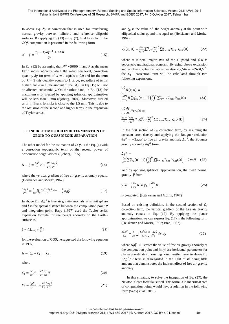
In above Eq. 𝛿𝛾 is correction that is used for transferring

normal gravity between telluroid and reference ellipsoid

surfaces. By applying Eq. (13) in Eq. (7), final formula for the

GQS computation is presented in the following form

𝑁 − 𝜁 =𝑇𝑔 − 𝑇𝑃𝛿𝛾

−1 + 𝐴𝐶𝐵

𝛾0 (15)

In Eq. (12) by assuming that 𝐻𝑁 ~5000 m and R as the mean

Earth radius approximating the mean sea level, correction

quantity 𝛿𝛾 for term of 𝑘 = 1 equals to 0.9 and for the term

of 𝑘 = 2 this quantity equals to 1. Ergo, regardless of terms

higher than 𝑘 = 1, the amount of the GQS in Eq. (15) will not

be affected substantially. On the other hand, in Eq. (12) the

maximum error created by applying spherical approximation

will be less than 1 mm (Sjoberg, 2004). Moreover, created

error in Bruns formula is close to the 1.5 mm. This is due to

the omission of the second and higher terms in the expansion

of Taylor series.

3. INDIRECT METHOD IN DETERMINATION OF

GEOID TO QUASIGEOID SEPARATION

The other model for the estimation of GQS is the Eq. (4) with

a correction topographic term of the second power of

orthometric height added, (Sjoberg, 1995).

𝑁 − 𝜁 =∆𝑔𝐵

�̅�𝐻 +

𝐻2

2�̅�

𝜕∆𝑔𝑃𝐹

𝜕𝐻 (16)

where the vertical gradient of free air gravity anomaly equals,

(Heiskanen and Moritz, 1967),

𝜕∆𝑔𝑃𝐹

𝜕𝐻=

𝑅2

2𝜋∬

∆𝑔𝐹−∆𝑔𝑃𝐹

𝑙3𝜎𝑑𝜎 −

2

𝑅∆𝑔𝑃

𝐹 (17)

In above Eq., ∆𝑔𝐹 is free air gravity anomaly, 𝜎 is unit sphere

and 𝑙 is the spatial distance between the computation point P

and integration point. Rapp (1997) used the Taylor series

expansion formula for the height anomaly on the Earth's

surface as

𝜁 = 𝜁0|𝑟=𝑟𝑒 +𝜕𝜁

𝜕𝑟ℎ (18)

for the evaluation of GQS, he suggested the following equation

in 1997,

𝑁 − [𝜁0 + 𝐶1] = 𝐶2 (19)

where

𝐶1 =𝜕𝜁

𝜕𝑟𝐻 +

𝜕𝜁

𝜕𝛾

𝜕𝛾

𝜕ℎ𝐻 (20)

𝐶2 =∆𝑔𝐵

𝛾𝐻 +

𝐻2

2𝛾

𝜕∆𝑔𝑃𝐹

𝜕𝐻 (21)

and 𝜁0 is the value of the height anomaly at the point with

ellipsoidal radius 𝑟𝑒 and it is equal to, (Heiskanen and Moritz,

1967),

𝜁0(𝑟𝑒 , Ω) =𝐺𝑀

𝑟𝑒𝛾0∑ (

𝑎

𝑟)𝑛∑ 𝑇𝑛𝑚𝑛𝑚=−𝑛 𝑌𝑛𝑚(Ω)

𝑀𝑛=2 (22)

where 𝑎 is semi major axis of the ellipsoid and GM is

geocentric gravitational constant. By using above expansion

and applying spherical approximation 𝜕𝛾 𝜕ℎ⁄ = −2𝐺𝑀 𝑟3⁄ ,

the 𝐶1 correction term will be calculated through two

following expansions.

𝜕𝜁

𝜕𝑟𝐻(𝑟, Ω) =

−𝐺𝑀

𝑟2𝛾0𝐻∑ (𝑛 + 1) (

𝑎

𝑟)𝑛


𝑛𝑚=−𝑛 𝑌𝑛𝑚(Ω) (23)

𝜕𝜁

𝜕𝛾

𝜕𝛾

𝜕ℎ𝐻(𝑟, Ω) =

2𝐺𝑀

𝑟3[𝐺𝑀

𝑟𝛾02𝐻 ∑ (

𝑎

𝑟)𝑛


𝑛𝑚=−𝑛 𝑌𝑛𝑚(Ω)] (24)

In the first section of 𝐶2 correction term, by assuming the

constant crust density and applying the Bouguer reduction

δ𝑔𝐵 = −2𝜋𝜇𝐻 to free air gravity anomaly ∆𝑔𝐹, the Bouguer

gravity anomaly ∆𝑔𝐵 from

∆𝑔𝐵 =

[𝐺𝑀

𝑟2∑ (𝑛 − 1) (

𝑎

𝑟)𝑛


𝑛𝑚=−𝑛 𝑌𝑛𝑚(Ω)] − 2𝜋𝜇𝐻 (25)

and by applying spherical approximation, the mean normal

gravity 𝛾 from

�̅� ≈ −1

2

𝜕𝛾

𝜕ℎ𝐻 ≈ 𝛾0 +

𝐺𝑀

𝑟3𝐻 (26)

is computed, (Heiskanen and Moritz, 1967).

Based on existing definition, in the second section of 𝐶2

correction term, the vertical gradient of the free air gravity

anomaly equals to Eq. (17). By applying the planer

approximation, we can express Eq. (17) in the following form

(Heiskanen and Moritz, 1967; Bian, 1997).

𝜕∆𝑔𝐹

𝜕𝐻=

1

2𝜋∬

∆𝑔𝐹(𝑥,𝑦)− ∆𝑔0𝐹

(𝑥2+𝑦2)32⁄𝑑𝑥 𝑑𝑦 (27)

where ∆𝑔0𝐹 illustrates the value of free air gravity anomaly at

the computation point and [𝑥, 𝑦] are horizontal parameters for

planer coordinates of running point. Furthermore, in above Eq.

2∆𝑔𝐹 𝑅⁄ term is disregarded in the light of its being little

amount that demonstrates the indirect effect of free air gravity

anomaly.

In this situation, to solve the integration of Eq. (27), the

Newton- Cotes formula is used. This formula in innermost area

of computation points would have a solution in the following

form (Sadiq et al., 2010).



491

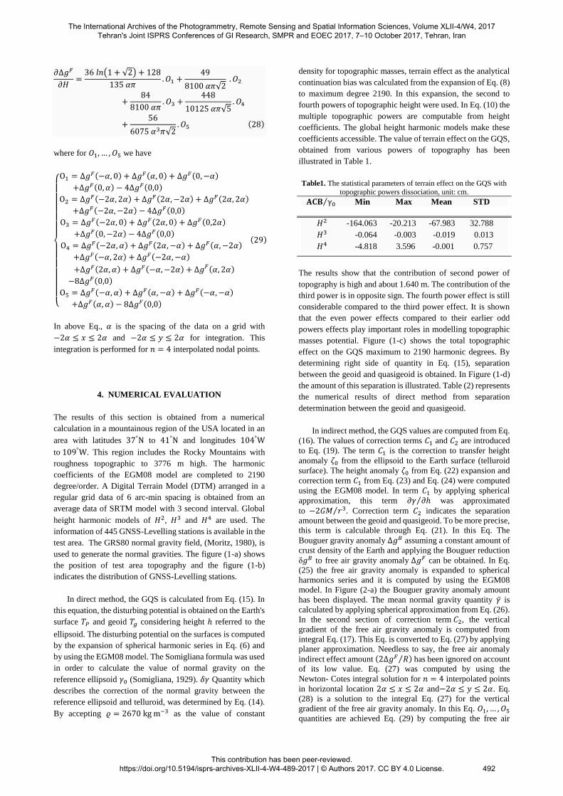
𝜕∆𝑔𝐹

𝜕𝐻=36 𝑙𝑛(1 + √2) + 128

135 𝛼𝜋. 𝛰1 +

49

8100 𝛼𝜋√2 . 𝛰2

+84

8100 𝛼𝜋. 𝛰3 +

448

10125 𝛼𝜋√5. 𝛰4

+56

6075 𝛼3𝜋√2. 𝛰5 (28)

where for 𝑂1, … , 𝑂5 we have

{

Ο1 = ∆𝑔

𝐹(−𝛼, 0) + ∆𝑔𝐹(𝛼, 0) + ∆𝑔𝐹(0,−𝛼)

+∆𝑔𝐹(0, 𝛼) − 4∆𝑔𝐹(0,0)

Ο2 = ∆𝑔𝐹(−2𝛼, 2𝛼) + ∆𝑔𝐹(2𝛼, −2𝛼) + ∆𝑔𝐹(2𝛼, 2𝛼)

+∆𝑔𝐹(−2𝛼,−2𝛼) − 4∆𝑔𝐹(0,0)

Ο3 = ∆𝑔𝐹(−2𝛼, 0) + ∆𝑔𝐹(2𝛼, 0) + ∆𝑔𝐹(0,2𝛼)

+∆𝑔𝐹(0,−2𝛼) − 4∆𝑔𝐹(0,0)

Ο4 = ∆𝑔𝐹(−2𝛼, 𝛼) + ∆𝑔𝐹(2𝛼, −𝛼) + ∆𝑔𝐹(𝛼,−2𝛼)

+∆𝑔𝐹(−𝛼, 2𝛼) + ∆𝑔𝐹(−2𝛼,−𝛼)

+∆𝑔𝐹(2𝛼, 𝛼) + ∆𝑔𝐹(−𝛼,−2𝛼) + ∆𝑔𝐹(𝛼, 2𝛼)

−8∆𝑔𝐹(0,0)

Ο5 = ∆𝑔𝐹(−𝛼, 𝛼) + ∆𝑔𝐹(𝛼, −𝛼) + ∆𝑔𝐹(−𝛼,−𝛼)

+∆𝑔𝐹(𝛼, 𝛼) − 8∆𝑔𝐹(0,0)

(29)

In above Eq., 𝛼 is the spacing of the data on a grid with

−2𝛼 ≤ 𝑥 ≤ 2𝛼 and −2𝛼 ≤ 𝑦 ≤ 2𝛼 for integration. This

integration is performed for 𝑛 = 4 interpolated nodal points.

4. NUMERICAL EVALUATION

The results of this section is obtained from a numerical

calculation in a mountainous region of the USA located in an

area with latitudes 37°N to 41°N and longitudes 104°W

to 109°W. This region includes the Rocky Mountains with

roughness topographic to 3776 m high. The harmonic

coefficients of the EGM08 model are completed to 2190

degree/order. A Digital Terrain Model (DTM) arranged in a

regular grid data of 6 arc-min spacing is obtained from an

average data of SRTM model with 3 second interval. Global

height harmonic models of 𝐻2, 𝐻3 and 𝐻4 are used. The

information of 445 GNSS-Levelling stations is available in the

test area. The GRS80 normal gravity field, (Moritz, 1980), is

used to generate the normal gravities. The figure (1-a) shows

the position of test area topography and the figure (1-b)

indicates the distribution of GNSS-Levelling stations.

In direct method, the GQS is calculated from Eq. (15). In

this equation, the disturbing potential is obtained on the Earth's

surface 𝑇𝑃 and geoid 𝑇𝑔 considering height ℎ referred to the

ellipsoid. The disturbing potential on the surfaces is computed

by the expansion of spherical harmonic series in Eq. (6) and

by using the EGM08 model. The Somigliana formula was used

in order to calculate the value of normal gravity on the

reference ellipsoid 𝛾0 (Somigliana, 1929). 𝛿𝛾 Quantity which

describes the correction of the normal gravity between the

reference ellipsoid and telluroid, was determined by Eq. (14).

By accepting 𝜚 = 2670 kg m−3 as the value of constant

density for topographic masses, terrain effect as the analytical

continuation bias was calculated from the expansion of Eq. (8)

to maximum degree 2190. In this expansion, the second to

fourth powers of topographic height were used. In Eq. (10) the

multiple topographic powers are computable from height

coefficients. The global height harmonic models make these

coefficients accessible. The value of terrain effect on the GQS,

obtained from various powers of topography has been

illustrated in Table 1.

Table1. The statistical parameters of terrain effect on the GQS with

topographic powers dissociation, unit: cm.

𝐀𝐂𝐁 γ0⁄ Min Max Mean STD

𝐻2 -164.063 -20.213 -67.983 32.788

𝐻3 -0.064 -0.003 -0.019 0.013

𝐻4 -4.818 3.596 -0.001 0.757

The results show that the contribution of second power of

topography is high and about 1.640 m. The contribution of the

third power is in opposite sign. The fourth power effect is still

considerable compared to the third power effect. It is shown

that the even power effects compared to their earlier odd

powers effects play important roles in modelling topographic

masses potential. Figure (1-c) shows the total topographic

effect on the GQS maximum to 2190 harmonic degrees. By

determining right side of quantity in Eq. (15), separation

between the geoid and quasigeoid is obtained. In Figure (1-d)

the amount of this separation is illustrated. Table (2) represents

the numerical results of direct method from separation

determination between the geoid and quasigeoid.

In indirect method, the GQS values are computed from Eq.

(16). The values of correction terms 𝐶1 and 𝐶2 are introduced

to Eq. (19). The term 𝐶1 is the correction to transfer height

anomaly 𝜁0 from the ellipsoid to the Earth surface (telluroid

surface). The height anomaly 𝜁0 from Eq. (22) expansion and

correction term 𝐶1 from Eq. (23) and Eq. (24) were computed

using the EGM08 model. In term 𝐶1 by applying spherical

approximation, this term 𝜕𝛾 𝜕ℎ⁄ was approximated

to −2𝐺𝑀 𝑟3⁄ . Correction term 𝐶2 indicates the separation

amount between the geoid and quasigeoid. To be more precise,

this term is calculable through Eq. (21). In this Eq. The

Bouguer gravity anomaly ∆𝑔𝐵 assuming a constant amount of

crust density of the Earth and applying the Bouguer reduction

δ𝑔𝐵 to free air gravity anomaly ∆𝑔𝐹 can be obtained. In Eq.

(25) the free air gravity anomaly is expanded to spherical

harmonics series and it is computed by using the EGM08

model. In Figure (2-a) the Bouguer gravity anomaly amount

has been displayed. The mean normal gravity quantity �̅� is

calculated by applying spherical approximation from Eq. (26).

In the second section of correction term 𝐶2, the vertical

gradient of the free air gravity anomaly is computed from

integral Eq. (17). This Eq. is converted to Eq. (27) by applying

planer approximation. Needless to say, the free air anomaly

indirect effect amount (2∆𝑔𝐹 𝑅⁄ ) has been ignored on account

of its low value. Eq. (27) was computed by using the

Newton- Cotes integral solution for 𝑛 = 4 interpolated points

in horizontal location 2𝛼 ≤ 𝑥 ≤ 2𝛼 and−2𝛼 ≤ 𝑦 ≤ 2𝛼. Eq.

(28) is a solution to the integral Eq. (27) for the vertical

gradient of the free air gravity anomaly. In this Eq. 𝑂1, … , 𝑂5

quantities are achieved Eq. (29) by computing the free air



492

gravity anomaly. In addition, the free air gravity anomalies in

a regular grid of data with spacing of 𝛼 = 6° are derived from

the EGM08 model. Figure (2-b) shows the vertical gradient of

the free air gravity anomaly in test area. By calculating right

side of quantity in Eq. (16) the GQS was obtained in the

indirect method. Figure (2-c) illustrates this separation. In

Table (3) the numerical results of this method were shown.

The GNSS-Levelling stations as the test points of known

GQS values are used to evaluate the accuracies of the direct

and indirect methods. Hence, the geoidal heights were

extracted from direct and indirect methods at the test points.

Table (4) illustrates the results of geoidal heights. As the

results show, the geoid modelled in direct and indirect methods

has on average 16 cm difference. This difference demonstrates

the models are comparable in centimeter accuracy level. In the

performed comparison between the obtained geoid from two

methods with the geometric geoid of GNSS-Levelling stations,

the direct method with 1.3 cm precision superiority in respect

to the indirect method at RMS scale is obvious. It has been

considered as an efficient method. In addition, this is indicated

as a precise approach in determining GQS. The stimulating

result of direct method is due to the precise modelling of

terrain effects. Comparison of the results of direct method in

the test area with the GNSS-Leveling results in the area shows

an average difference of 7 cm in GQS values. Also, the Chi-

squared goodness of fit test shows the normal distribution of

the residuals in the test area.

Figure 1. (a) the topographic of test area, unit: meter, (b) GNSS-Levelling stations location in test area, (c) the total topographic

effect on the GQS, unit: meter and (d) separation between the geoid to quasigeoid as a result of the direct method, unit: meter.

b a

c d



493

Table 2. The statistical characteristics of GQS based on direct method, unit: meter.

Figure 2. (a) The Bouguer gravity anomaly with 6 arc-min interval, unit: mGal, (b) the vertical gradient of the free air gravity

anomaly with 6 arc-min interval, unit: mGal and (c) the GQS obtained from indirect method, unit: m.

Table 3. The statistical parameters of GQS based on indirect method.

Statistical parameters Min Max Mean STD

𝑇𝑔 𝛾0⁄ -20.679 -9.860 -15.076 2.472

𝑇𝑃𝛿𝛾−1 𝛾0⁄ -20.674 -9.969 -15.126 2.438

𝐴𝐶𝐵 𝛾0⁄ -1.685 -0.201 -0.680 0.331

𝑁 − 𝜁 -1.581 -0.066 -0.629 0.299

Statistical parameters Min Max Mean STD

∆𝑔𝐹[mGal] -106.868 249.239 26.176 54.125

𝛿𝑔𝐵 [mGal] -422.712 -149.532 -264.496 64.435

∆𝑔𝐵[mGal] -415.857 -87.203 -238.320 48.765

𝜕∆𝑔𝐹 𝜕𝐻⁄ [mGal] -0.022 0.015 0.000 0.004

𝐶1 [m] -0.524 0.148 -0.079 0.123

[𝜁0 + 𝐶1] = 𝜁 [m] -20.630 -10.289 -15.195 2.365

𝑁 − 𝜁 = 𝐶2 [m] -1.322 -0.212 -0.596 0.236

a b

c



494

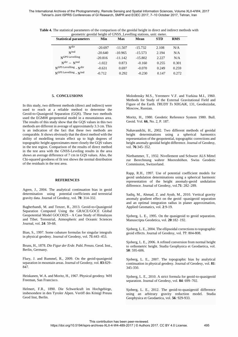
Table 4. The statistical parameters of the comparison of the geoidal height in direct and indirect methods with

geometric geoidal height of GNSS_Levelling stations, unit: meter.

5. CONCLUSIONS

In this study, two different methods (direct and indirect) were

used to reach at a reliable method to determine the

Geoid-to-Quasigeoid Separation (GQS). These two methods

used the EGM08 geopotential model in a mountainous area.

The results of this study show that the GQS values in this two

methods are different in average of approximately 3.3 cm. This

is an indication of the fact that these two methods are

comparable. It shows obviously that the direct method with the

ability of modelling terrain effect up to high degrees of

topographic height approximates more closely the GQS values

in the test region. Comparison of the results of direct method

in the test area with the GNSS-Leveling results in the area

shows an average difference of 7 cm in GQS values. Also, the

Chi-squared goodness of fit test shows the normal distribution

of the residuals in the test area.

REFERENCES

Agren, J., 2004. The analytical continuation bias in geoid

determination using potential coefficients and terrestrial

gravity data. Journal of Geodesy, vol. 78: 314-332.

Bagherbandi, M. and Tenzer, R., 2013. Geoid-to-Quasigeoid

Separation Computed Using the GRACE/GOCE Global

Geopotential Model GOCO02S - A Case Study of Himalayas

and Tibet. Terrestrial, Atmospheric and Oceanic Sciences

Journal, vol. 24: 59-68.

Bian, S., 1997. Some cubature formulas for singular integrals

in physical geodesy. Journal of Geodesy, vol. 71:443–453.

Bruns, H., 1878. Die Figur der Erde. Publ. Preuss. Geod. Inst.,

Berlin, Germany.

Flury, J. and Rummel, R., 2009. On the geoid-quasigeoid

separation in mountain areas. Journal of Geodesy, vol. 83:829–

847.

Heiskanen, W.A. and Moritz, H., 1967. Physical geodesy. WH

Freeman, San Francisco.

Helmert, F.R., 1890. Die Schwerkraft im Hochgebirge,

insbesondere in den Tyroler Alpen. Veröff des Königl Preuss

Geod Inst, Berlin.

Molodensky M.S., Yeremeev V.F. and Yurkina M.I., 1960.

Methods for Study of the External Gravitational Field and

Figure of the Earth. TRUDY Ts NIIGAiK, 131, Geodezizdat,

Moscow, Russian.

Moritz, H., 1980. Geodetic Reference System 1980. Bull.

Geoid. Vol. 66, No. 2, P. 187.

Nahavandchi, H., 2002. Two different methods of geoidal

height determinations using a spherical harmonics

representation of the geopotential, topographic corrections and

height anomaly-geoidal height difference. Journal of Geodesy,

vol. 76:345–352.

Niethammer, T., 1932. Nivellement und Schwere ALS Mittel

zur Berechnung wahrer Meereshöhen. Swiss Geodetic

Commission, Switzerland.

Rapp, R.H., 1997. Use of potential coefficient models for

geoid undulation determinations using a spherical harmonic

representation of the height anomaly-geoid undulation

difference. Journal of Geodesy, vol.71: 282–289.

Sadiq, M., Ahmad, Z. and Ayub, M., 2010. Vertical gravity

anomaly gradient effect on the geoid -quasigeoid separation

and an optimal integration radius in planer approximation,

Applied Geomatics, vol. 2:9-19.

Sjoberg, L. E., 1995. On the quasigeoid to geoid separation.

Manuscripta Geodetica, vol. 20:182–192.

Sjoberg, L. E., 2004. The ellipsoidal corrections to topographic

geoid effects. Journal of Geodesy, vol. 77: 804-808.

Sjoberg, L. E., 2006. A refined conversion from normal height

to orthometric height. Studia Geophysica et Geodaetica, vol.

50: 595-606.

Sjoberg, L. E., 2007. The topographic bias by analytical

continuation in physical geodesy. Journal of Geodesy, vol. 81:

345-350.

Sjoberg, L. E., 2010. A strict formula for geoid-to-quasigeoid

separation. Journal of Geodesy, vol. 84: 699–702.

Sjoberg, L. E., 2012. The geoid-to-quasigeoid difference

using an arbitrary gravity reduction model. Studia

Geophysica et Geodaetica, vol. 56: 929-933.

Statistical parameters Min Max Mean STD RMS

Ndir -20.697 -11.507 -15.732 2.108 N/A

Nind -20.640 -10.965 -15.573 2.194 N/A

NGPS Levelling -20.816 -11.142 -15.802 2.227 N/A

Ndir − Nind -1.022 0.873 -0.160 0.255 0.301

NGPS Levelling - Ndir -0.631 0.697 -0.070 0.249 0.259

NGPS Levelling - Nind -0.712 0.292 -0.230 0.147 0.272



495

Sjoberg, L. E. and Bagherbandi, M., 2012. Quasigeoid-to-

geoid determination by EGM08. Earth Science Informatics,

vol. 5: 87-91.

Sjoberg, L. E., 2015. Rigorous geoid-from-quasigeoid

correction using gravity disturbances. Journal of Geodetic

Science. vol. 5:115–118.

Somigliana, C., 1929. Teoria Generale del Campo

Gravitazionale dell’Ellisoide di Rotazione Memoire Della

Societa Astronomica Italiana, IV.

Tenzer, R., Novák, P., Moore, P., Kuhn, M. and Vanicek, P.,

2006. Explicit formula for the geoid-quasigeoid separation.

Studia Geophysica et Geodaetica, vol. 50: 607-618.


This contribution has been peer-reviewed. https://doi.org/10.5194/isprs-archives-XLII-4-W4-489-2017 | © Authors 2017. CC BY 4.0 License. 496

Documents

ON THE COMPUTATION OF A PRECISE GEOID TO QUASIGEOID …