Embed Size (px)
Citation preview
On the Complexity of CountingIrreducible Components and Computing
Betti Numbers of Algebraic Varieties
Dissertation
zur Erlangung des Doktorgradesder Fakultat fur Elektrotechnik, Informatik und Mathematik
der Universitat Paderborn
vorgelegt von
Peter Scheiblechner
Paderborn, den 12. Juli 2007

ii

iii
iv
Fur Pia,Pino undClara
Gutachter: Prof. Dr. Peter BurgisserProf. Dr. Felipe CuckerProf. Dr. Joachim von zur Gathen
Abstract
This thesis is a continuation of the study of counting problems in algebraicgeometry within an algebraic framework of computation started by Burgisser,Cucker, and Lotz in a series of papers [BC03, BC06, BCL05].
In its first part we give a uniform method for the two problems #CCCand #ICC of counting the connected and irreducible components of complexalgebraic varieties, respectively. Our algorithms are purely algebraic, i.e., theyuse only the field structure of C. They work in parallel polynomial time, i.e.,they can be implemented by algebraic circuits of polynomial depth. The designof our algorithms relies on the concept of algebraic differential forms. A furtherimportant building block is an algorithm of Szanto [Sza97] computing a variantof characteristic sets.
The second part contains lower bounds in terms of hardness results for topo-logical problems dealing with complex algebraic varieties. In particular, we showthat the problem of deciding connectedness of a complex affine or projective va-riety given over the rationals is PSPACE-hard. We further extend this result tohigher Betti numbers. More precisely, we prove that it is also PSPACE-hard todecide whether a Betti number of fixed order of a complex affine or projectivevariety is less than some given integer.
In the third part we study the dependency of the complexity of #ICC on itscombinatorial parameters. The crucial complexity parameter for the problemturns out to be the number of equations. This fact is illustrated by our resultabout counting the absolutely irreducible factors of a multivariate polynomial,the restriction of the general problem to the case of a single equation. We showthat one can solve this problem in parallel polylogarithmic time.
Furthermore, we describe a generic parsimonious reduction of the prob-lem #ICC for a fixed number of equations to a fixed number of variables. Theconsequences are that one can solve #ICC for a fixed number of equations inthe BSS-model in polynomial time, and in the Turing model in randomisedparallel polylogarithmic time. These results hold also for polynomials given bystraight-line programs using their length and the degree as input parameters.
v

vi
Danksagungen
Mein allergroßter Dank gilt meinem Doktorvater Peter Burgisser fur sein Ver-trauen und dafur, dass er mir die Moglichkeit der Promotion gegeben hat, seinesehr gute und immer freundliche Betreuung und Unterstutzung in vielerlei Hin-sicht, und alles, was ich von ihm (auch außermathematisch) gelernt habe. Weit-erhin herzlich bedanken mochte ich mich bei Thilo Pruschke fur das Finden einesFehlers und hilfreiche Diskussionen uber das Hilbertpolynom. Außerdem habenmir meine Arbeitsgruppenkollegen Martin Lotz und Martin Ziegler mit einerangenehmen Arbeitsatmosphare und vielen wertvollen Gesprachen geholfen.
Nicht zuletzt bedanke ich mich ganz herzlich bei meiner Familie, insbeson-dere bei Pia fur ihre endlose Geduld und Toleranz.
Diese Arbeit wurde durch die DFG Sachbeihilfe BU 1371 unterstutzt.

Contents
0 Introduction 10.1 General Upper Bounds . . . . . . . . . . . . . . . . . . . . . . . . 20.2 Lower Complexity Bounds . . . . . . . . . . . . . . . . . . . . . . 70.3 Fixing Parameters . . . . . . . . . . . . . . . . . . . . . . . . . . 90.4 Outline . . . . . . . . . . . . . . . . . . . . . . . . . . . . . . . . 130.5 Credits . . . . . . . . . . . . . . . . . . . . . . . . . . . . . . . . . 14
1 Preliminaries 171.1 Algebraic Geometry . . . . . . . . . . . . . . . . . . . . . . . . . 171.2 Differential Forms . . . . . . . . . . . . . . . . . . . . . . . . . . 231.3 Models of Computation . . . . . . . . . . . . . . . . . . . . . . . 271.4 Structural Complexity . . . . . . . . . . . . . . . . . . . . . . . . 321.5 Efficient Parallel Algorithms . . . . . . . . . . . . . . . . . . . . . 351.6 Squarefree Regular Chains . . . . . . . . . . . . . . . . . . . . . . 39
I Upper Bounds 43
2 Transfer Results 452.1 Transfer Results for Complexity Classes . . . . . . . . . . . . . . 452.2 Generic and Randomised Reductions . . . . . . . . . . . . . . . . 49
3 Counting Connected Components 553.1 The Zeroth de Rham Cohomology . . . . . . . . . . . . . . . . . 563.2 Modified Pseudo Remainders . . . . . . . . . . . . . . . . . . . . 593.3 Computing Differentials . . . . . . . . . . . . . . . . . . . . . . . 623.4 Proof of Theorem 3.1 . . . . . . . . . . . . . . . . . . . . . . . . . 65
4 Counting Irreducible Components 674.1 Affine vs. Projective Case . . . . . . . . . . . . . . . . . . . . . . 684.2 Locally Constant Rational Functions . . . . . . . . . . . . . . . . 694.3 Proof of Theorem 4.1 . . . . . . . . . . . . . . . . . . . . . . . . . 71
5 Hilbert Polynomial 755.1 Bound for the Index of Regularity . . . . . . . . . . . . . . . . . 765.2 Computing the Hilbert Polynomial . . . . . . . . . . . . . . . . . 78
vii

viii CONTENTS
II Lower Bounds 81
6 Connectedness 836.1 Basic Notations . . . . . . . . . . . . . . . . . . . . . . . . . . . . 836.2 Obtaining an Acyclic Configuration Graph . . . . . . . . . . . . . 846.3 Embedding the Configuration Graph . . . . . . . . . . . . . . . . 866.4 Equations for the Embedded Graph . . . . . . . . . . . . . . . . 896.5 Proof of Theorem 6.1 . . . . . . . . . . . . . . . . . . . . . . . . . 946.6 Appendix. The Real Reachability Problem . . . . . . . . . . . . 95
7 Betti Numbers 977.1 The Affine Case . . . . . . . . . . . . . . . . . . . . . . . . . . . . 977.2 The Projective Case . . . . . . . . . . . . . . . . . . . . . . . . . 98
III Fixing Parameters 103
8 Counting Irreducible Factors 1058.1 Cohomology of a Hypersurface Complement . . . . . . . . . . . . 1068.2 Structure Theorem for Closed 1-Forms . . . . . . . . . . . . . . . 1078.3 Proof of Theorem 8.3 . . . . . . . . . . . . . . . . . . . . . . . . . 1108.4 Characterising Exact Forms . . . . . . . . . . . . . . . . . . . . . 1128.5 Proof of Theorem 8.1 . . . . . . . . . . . . . . . . . . . . . . . . . 1148.6 Counting Irreducible Components Revisited . . . . . . . . . . . . 115
9 Fixed Number of Equations 1179.1 Proof of the Main Results . . . . . . . . . . . . . . . . . . . . . . 1179.2 Transversality . . . . . . . . . . . . . . . . . . . . . . . . . . . . . 1199.3 Explicit Genericity Condition for Bertini . . . . . . . . . . . . . . 1229.4 Expressing the Genericity Condition . . . . . . . . . . . . . . . . 129

Chapter 0
Introduction
A common principle in many mathematical areas is the possibility to constructcomplicated objects out of simpler ones. Ideally there exists some set of “sim-plest” objects in the sense that they cannot be built up by even simpler ones;these are called prime or irreducible. An elementary and well-known example ofthis principle is the factorisation of integers into a product of prime numbers.For example,
156 = 22 · 3 · 13
is the factorisation of 156 into prime numbers. As one sees in this example, it iseasy to combine (multiply) the prime numbers to obtain the resulting number.Conversely, the “inverse” problem of constructing the factorisation from theresult seems to be a much harder (hence much more interesting) task.
This thesis adresses such inverse problems in the realm of complex algebraicgeometry. Structurally very similar to factorisation of integers is the factori-sation of polynomials into irreducible ones. This seemingly algebraic problemis a special case of the decomposition problem of an algebraic variety into ir-reducible components. This also has a geometric flavour as the decompositionproblem of a topological space (e.g., an algebraic variety) into connected com-ponents. More specifically, these problems are studied from a computationalcomplexity point of view, i.e., we try to figure out how hard they are to solvealgorithmically. One aim of this research is to identify complexity classes suchas P or PSPACE, for which the problems are complete. Here P and PSPACEdenote the class of decision problems decidable in polynomial time and space,respectively [Joh90, Pap94]. That a problem A is complete for the class C meansthat it is among the hardest problems in C. This is a twofold statement:
• A is as most as hard as the problems in C, i.e., it lies in C;
• A is as least as hard as any problem B from C in the sense that an efficientalgorithm solving A also solves B efficiently.
The first of these statements is also called an upper bound and the second alower bound for A.
In complexity theory it is convenient to restrict oneself to problems asking forthe existence (decision problems) or the number of solutions (counting problems)of some question. We will focus on the counting versions of our problems.
1

2 CHAPTER 0. INTRODUCTION
0.1 General Upper Bounds
The problems we prove upper bounds for are specified as follows.
#CCC (Counting connected components) Given finitely many complex poly-nomials, compute the number of connected components of their affine zero set.
#ICC (Counting irreducible components) Given finitely many complex poly-nomials, compute the number of irreducible components of their affine zero set.
To be specific we use for the problem #CCC the Euclidean topology andfor #ICC the Zariski topology. We discuss these problems in two models ofcomputation. The first one is the model of algebraic circuits, which are capableof doing complex arithmetic exactly with unit cost. This is a standard modelin algebraic complexity theory. Adding uniformity conditions it is equivalentto the BSS model named after Blum, Shub, and Smale [BSS89]. The secondmodel is the discrete model of Boolean circuits. In order to study our problemsin the discrete model, we restrict their inputs to rational polynomials whosecoefficients are thought of as pairs of binary numbers. These restricted versionsare denoted by #CCQ and #ICQ, respectively.
Both algebraic and Boolean circuits serve as models for parallel computation,since the depth of a circuit can be interpreted as the running time when thereare enough processors evaluating the gates of the circuit in parallel (ignoringcommunication and synchronisation cost). According to this observation werefer to the depth of a circuit as the parallel and to its size as the sequentialrunning time of the algorithm modelled by the circuit. Using this terminologywe can state our general upper bound results as follows.
Theorem 0.1. The problems #CCC and #ICC can be solved in parallel poly-nomial and sequential exponential time. The same is true for #CCQ and #ICQin the discrete setting.
0.1.1 Counting Connected Components
The basic mathematical ideas behind the algorithms proving Theorem 0.1 arevery classic. We first focus on the problem #CCC. It is well-known frompoint-set topology that the connected components of a topological space Xcan be characterised by the locally constant functions on X. More precisely,the number of connected components of X equals the dimension of the vectorspace H0(X) of locally constant functions on X. In the case of an algebraicvariety V ⊆ Cn we would like to work with functions given by polynomials, i.e.,regular functions on V . To see that one can realise each locally constant functionby a polynomial, we prove a direct product decomposition of the coordinatering C[V ] = C[X1, . . . , Xn]/I of V , where I := I(V ) is the vanishing idealof V . Let V =
⋃i Vi be the decomposition into connected components, and
Ii := I(Vi). Then I =⋂
i Ii. By Hilbert’s Nullstellensatz, Vi ∩ Vj = ∅ impliesIi + Ij = C[X1, . . . , Xn] for i 6= j. The Chinese Remainder Theorem yields theisomorphism
C[V ] '∏
i
C[Vi]. (1)

0.1. GENERAL UPPER BOUNDS 3
Since each locally constant function on V must be constant on each Vi, by (1)it can also be represented on V by a polynomial.
But what does all this help algorithmically? One could try to find thedecomposition (1) using the characterisation of the direct product by a completeset eii of orthogonal idempotents, i.e.,
e2i = ei, eiej = 0,∑
i
ei = 1 for all i 6= j.
But these conditions correspond to a non-linear system of equations of exponen-tial size, since the number of connected components is exponential in the worstcase. However, the exponential size would not bother us in the case of a linearsystem of equations, since linear algebra can be done in parallel polylogarithmictime. In fact, we can prove a single exponential degreee bound for the ei withthe help of the effective Nullstellensatz [Bro87, Kol88].
As a means to linearise these conditions we use the characterisation of locallyconstant functions by their vanishing differential, an idea coming from differen-tial topology. For the possibly singular algebraic variety V one has to be carefulabout the notion of differentials. We use the Kahler differential df of a regularfunction f ∈ C[V ]. With this notion it is also true that f is locally constantif and only if df = 0. Our aim is to write this condition as a linear system ofequations in the coefficients of f .
Fortunately there is a concept helping us in this task, namely the notion ofsquarefree regular chains. We briefly sketch their definition and basic properties.A triangular set G = g1, . . . , gt is a set of polynomials such that each gi
introduces a new variable called the main variable. The saturated ideal of G isSat (G) := (G) : Γ∞, where Γ is the product of the leading coefficients lc (gi) ofthe gi with respect to their main variables. If no lc (gi) is a zerodivisor modulothe saturated ideal of Gi−1 := g1, . . . , gi−1, then G is called a regular chain.If in addition the gi are squarefree modulo each associated prime of Sat (Gi−1),G is called a squarefree regular chain. These increasingly restrictive conditionson G induce some nice properties on its saturated ideal. To formulate these, weneed the following notation. The pseudo division of a polynomial f by g withrespect to some variable Xi is obtained by applying univariate division withremainder to f and g regarded as univariate polynomials in Xi and clearingdenominators by multiplication with a suitable power of the leading coefficientof g. The pseudo remainder prem (f,G) of f by the triangular set G is the lastremainder obtained by pseudo dividing f successively by gt, . . . , g1 with respectto their main variables. Then the following statements hold [ALM99, BLM06].
• G triangular set ⇒ Sat (G) unmixed,
• G regular chain ⇒ Sat (G) = f |prem (f,G) = 0,
• G squarefree regular chain ⇒ Sat (G) radical.
It follows that for a squarefree regular chain G a polynomial f vanishes onZ(Sat (G)) if and only if prem (f,G) = 0. By fixing the exponent in the defini-tion of pseudo division this condition becomes linear in f .
Now it is a rather special situation when a variety V is represented by asquarefree regular chain. But Agnes Szanto proved in her thesis [Sza97, Sza99]

4 CHAPTER 0. INTRODUCTION
the following strong result which is crucial for us. The vanishing ideal of eachaffine variety V can be decomposed into an intersection
I(V ) =⋂i
Sat (Gi)
with squarefree regular chains Gi (which she called unmixed ascending sets).Furthermore, this representation can be computed in parallel polynomial time.Using this algorithm we can indeed describe the “truncated ideal” I(V ) ∩C[X]≤d, which consists of the polynomials in I(V ) of degree bounded by d,by a linear system of equations of single exponential size, if d is single exponen-tial. In this way we can also describe the space H0(V ) by such systems, so thatits dimension can be computed efficiently.
0.1.2 Counting Irreducible Components
We approach the problem #ICC analogously to #CCC. The key idea is toreplace regular by rational functions on the variety V . The ring R(V ) of ra-tional functions on V is defined to be the full quotient ring of the coordinatering C[V ], i.e., its localisation with respect to the multiplicatively closed sub-set of non-zerodivisors. In particular, we use that the number of irreduciblecomponents of V is the dimension of the space of locally constant rational func-tions on V . This is implied by the following direct product decomposition ofthe ring R(V ) [Kun79, III, Satz 2.8], which is analogue to the one of C[V ]. IfV =
⋃i Vi is the decomposition into irreducible components, then
R(V ) '∏
i
R(Vi).
The idempotents corresponding to this decomposition are rational functionsvanishing on all but one component, where they take the value 1. Thus they arelocally constant, and it is easy to see that they constitute a basis of the spaceof locally constant rational functions
H0r (V ) := f ∈ R(V ) |df = 0.
Hence the number of irreducible components of V is given by dimC H0r (V ).
Unfortunately, the equation obtained by clearing denominators in df = 0 isnon-linear (there appear products of the numerator and derivatives of the de-nominator and vice versa). But of course it is linear in the numerator alone for afixed denominator, hence we need a common denominator h of the idempotents.
Such an h ∈ C[V ] is a non-zerodivisor in C[V ], i.e., it does not vanishidentically on any Vi. Furthermore, on the intersection of two components atleast two of the idempotents are not defined. Hence a necessary condition for his that
h is a non-zerodivisor in C[V ] and h ∈⋂i 6=j
I(Vi ∩ Vj). (2)
On the other hand, if h ∈ C[V ] satisfies (2), then
U := V \ Z(h) =⋃i
(Vi \ Z(h))

0.1. GENERAL UPPER BOUNDS 5
is the decomposition into connected components, since the irreducible vari-eties Vi are connected [Sha77, VII, §2.2]. Using the well-known Rabinowitchtrick one obtains from the corresponding result for C[U ] the idempotents ofR(V ) in C[V ]h as well as a single exponential degree bound. Now one canwrite the defining equation for H0
r (V ) as a linear system of equations in thecoefficients of the numerator and apply efficient linear algebra.
To summarise, all we need is an h with (2) to proceed similarly to the caseof connected components. Fortunately, such an h is obtained from a squarefreeregular chain as follows. Assume for simplicity that I(V ) is the saturated ideal ofa squarefree regular chain G = g1, . . . , gt. Then the product Γ =
∏i lc (gi) is a
non-zerodivisor on C[V ]. We further denote with ∆ the functional determinantof (g1, . . . , gt) with respect to the free variables (those which are not the mainvariable of some gi). Using the squarefreeness condition one can prove that ∆is neither a zerodivisor. It follows that h := Γ∆ satisfies (2), since all points ofV \ Z(∆) can be shown to be smooth, and
⋃i 6=j Vi ∩ Vj ⊆ Sing (V ).
0.1.3 Hilbert Polynomial
As a by-product of our method for counting the connected and irreducible com-ponents we show how to obtain a parallel polynomial time algorithm computingthe Hilbert polynomial of a projective variety which is arithmetically Cohen-Macaulay. The general problem of computing the Hilbert polynomial of a com-plex projective variety still lacks a parallel polynomial time solution.
The idea of our algorithm is that with the help of squarefree regular chainsand Szantos algorithm [Sza97] we can compute the dimension of the homoge-neous part of degree d of the ideal of a projective variety in parallel polynomialtime, as long as d is single exponential in the input size. Hence we can evaluateits Hilbert function at single exponential arguments. Now one can compute theHilbert polynomial by interpolating the Hilbert function at sufficiently manypoints. The number of points needed is the dimension of the variety, so the crit-ical parameter for the complexity of our algorithm is the index, from which onthe Hilbert function agrees with the Hilbert polynomial. The minimal numberwith this property is called the index of regularity or a-invariant in the litera-ture [SV86, Vas98]. This quantity is closely related to the Castelnuovo-Mumfordregularity (cf. [BM93]). Unfortunately, a single exponential bound for the indexof regularity of a radical is not known. By a standard argument we prove sucha bound for a projective arithmetically Cohen-Macaulay variety. Consequentlyone can compute in this case the Hilbert polynomial in parallel polynomial time.
0.1.4 Related Work
The algorithmic problem of getting connectivity information about semialge-braic sets is well-studied, see Basu et al. [BPR03] and the numerous citationsgiven there. In particular, work of Canny [Can88] yields algorithms countingthe connected components of a semialgebraic set given by rational polynomi-als in polynomial space (and thus in single exponential time). By separatingreal and imaginary parts these methods can be applied to complex algebraicvarieties as well. However, these algorithms use the ordering of the real fieldin an essential way, in particular sign tests are allowed. Thus it remained an

6 CHAPTER 0. INTRODUCTION
open problem whether one can efficiently count the connected components of acomplex algebraic variety by only algebraic methods.
Concerning higher Betti numbers it is an important open problem whetherone can compute all Betti numbers of an algebraic variety in single exponen-tial time. The best result in this direction has been recently obtained byBasu [Bas06], who showed that for each fixed ` one can compute the first `Betti numbers in single exponential time. It is not yet clear whether thisalgorithm can be parallelised. Algebraic algorithms computing the cohomol-ogy of projective varieties and complements of affine varieties are describedin [OT99, Wal00a, Wal00b] but not analysed.
The computational tool in our algorithm which we call squarefree regularchain is one of various variants of the notion of characteristic sets, which goesback to Ritt [Rit50] and was used by Wu [Wu86] for automated theorem proving.Its computational complexity was studied by Gallo and Mishra [GM91]. Sub-sequently, algorithms computing variants of this concept were studied by Kalk-brener [Kal93, Kal94, Kal98], Lazard [Laz91], and Wang [Wan92]. Szanto [Sza97,Sza99] has further refined the methods of Kalkbrener to obtain a provably ef-ficient algorithm. Since at that time there existed several similar notions ofcharacteristic sets under different names and different concepts under the samename, Aubry et al. [ALM99] started a comparison of these different notionsand showed that some of them are basically equivalent. They also introduceda consistent naming convention we think one should follow to avoid confusion.In [BLM06] it is shown that the saturated ideal of a triangular set is unmixed.
Considering the problem of computing irreducible decompositions one hasto distinguish irreducible and absolutely irreducible decompositions. Irreduciblecomponents are irreducible over the ground field over which the variety is de-fined (e.g. the rationals), whereas the components irreducible over the algebaicclosure of the ground field are called absolutely irreducible. There are decom-position algorithms based on characteristic sets [Wu86, Laz91, Kal94]. Thesecompute decompositions which are not minimal in general, and also there areno complexity estimates of these algorithms. Other methods compute (modulofactorisation) the primary decomposition using Grobner bases [GTZ88, EHV92],but according to Mayr [MM82] (see also [May97]), computing those is exponen-tial space-complete. The first single exponential time algorithms for computingboth the irreducible and absolutely irreducible components are due to Chistovand Grigoriev [Chi84, Gri84] (in the bit model). Giusti and Heintz [GH91a] suc-ceeded in giving efficient parallel algorithms, but only for the equidimensionaldecomposition due to the lack of efficient parallel factorisation procedures. Adifferent approach using the Bezoutian matrix has been proposed in [EM99].However, their algorithm produces embedded components.
Algorithms computing the Hilbert polynomial of a complex projective varietyhave been given in [MM83, BCR91, BS92] and are based on Grobner bases,hence they show the same worst-case behaviour as the algorithms for primarydecomposition mentioned above. For the restriced problem of computing theHilbert polynomial of smooth equidimensional complex varieties Burgisser andLotz [BL07] have given a parallel polynomial time algorithm. In fact, they haveshown the stronger statement that this problem is reducible in polynomial timeto counting the solutions of systems of polynomial equations.

0.2. LOWER COMPLEXITY BOUNDS 7
0.2 Lower Complexity Bounds
We prove lower bounds in terms of hardness results in the Turing model, hencewe consider affine as well as projective varieties given over the rationals. Tomake our results stronger we consider decision versions of our problems.
0.2.1 Connectedness
Our first decision problem is the following.
ConnQ (Connectedness of affine varieties) Given finitely many rationalpolynomials, decide whether their affine zero set is connected.
The corresponding hardness result is
Theorem 0.2. The problem ConnQ is PSPACE-hard.
We will also prove a projective version of this theorem and conclude thatthe corresponding counting problems are FPSPACE-hard.
Our proof of this theorem uses the strategy of [BC03], [BC06], and [BCdN06]together with some new ideas. Burgisser and Cucker used the fact that eachlanguage in PSPACE can be decided by a symmetric Turing machine. Sucha machine has a symmetric transition function and thus an undirected con-figuration graph. Hence deciding membership to the language is reduced totesting whether two given vertices in an undirected graph are connected, i.e.,to the reachability problem. Note that this graph has an exponential numberof vertices, but it can be described succinctly, i.e., by a Boolean circuit whichdecides adjacency of two given vertices. This configuration graph was repre-sented in [BC03] as a semilinear set by mapping the vertices to points in realaffine space and edges to the line segments between them. One can show thatmembership to this set can be decided by an additive circuit of polynomial size.In this way the reachability problem translates to the reachability problem in asuccinctly given semilinear set, which in turn can be reduced to the problem ofcounting connected components as follows. One connects the two given pointsby new line segments obtaining a new semilinear set. Then the two points areconnected in the original set if and only if the number of connected componentsdoes not change by this modification.
We modify this strategy in several respects. We avoid the use of symmet-ric Turing machines by observing that one can simply pass to the underlyingundirected graph, since we are dealing with deterministic Turing machines (cf.Lemma 6.2). To be able to reduce to the problem of connectedness we constructfrom the given Turing machine a two-tape machine with an acyclic configurationgraph (cf. Lemma 6.3). Here special attention has to be paid to those configu-rations, which occur in no computation from any input. In this way, at the costof a second tape, we gain the ability to transform the configuration graph intoa forest of two trees. In this situation the reachability problem can easily bereduced to deciding connectedness. Since we are dealing with complex varieties,we embed these graphs into the complex affine or projective space by mappingedges to complex lines.

8 CHAPTER 0. INTRODUCTION
0.2.2 Betti Numbers
To formulate the generalisation to higher Betti numbers we introduce the fol-lowing problems. For a topological space X we denote by bk(X) its kth Bettinumber with respect to singular homology.
Betti(k)Q (kth Betti number of affine varieties) Given finitely many ra-tional polynomials with affine zero set X and b ∈ N, decide whether bk(X) ≤ b.
ProjBetti(k)Q (kth Betti number of projective varieties) Given finitelymany homogeneous rational polynomials with projective zero set X and b ∈ N,decide whether bk(X) ≤ b.
Now we can state our second hardness result.
Theorem 0.3. The problems Betti(k)Q and ProjBetti(k)Q are PSPACE-hard.
We prove this theorem by induction on k. Clearly, the case k = 0 followsfrom the result about ConnC and its projective version. The induction stepin the affine case is quite elementary and uses the idea of a similar result forsemilinear sets given by additive circuits in [BC03].
For the projective result we treat the case k = 1 separately with the samereduction as for the case k = 0 by observing that an additional edge fromthe leaf of a tree to its root introduces a cycle, whereas it does not, whenthe leaf is connected to the root of another tree. For the induction step wereduce ProjBetti(k)Q to ProjBetti(k + 2)Q. This reduction consists of theconstruction of the (algebraic) suspension Σ(X) of a projective variety X ⊆ Pn,which is defined as the join of X with an additional point p outside of Pn, i.e.,the union of all lines connecting p with a point of X (see Figure 1). As anillustration consider the following toy example. Take X as being two distinctpoints in Pn. Then the join of X with p is nothing else as the union of two linesmeeting in p, thus topologically S2 ∨ S2. One sees in this simple example thatthe zeroth Betti number of X agrees with the second Betti number of Σ(X).This shift of the Betti numbers by 2 is generally true. This fact is shown inAppendix A.6, p. 78 of [FM94] for the more general construction of an m-foldcone (where the Betti numbers are shifted by 2m), but only for the special caseof a smooth variety. Here we will prove this result for possibly singular varietiesfor m = 1. In order to do so, we will construct the blow-up of Σ(X) at p andshow that this is a sphere bundle over X, whose homology can be computedwith standard tools (see Figure 2).
0.2.3 Related Work
There is much less work on lower bounds than on upper bounds for topologicalproblems. It follows from work of Reif [Rei79, Rei87] that computing the numberof connected components of a semialgebraic set given by integer polynomials isFPSPACE-hard, hence this problem is FPSPACE-complete. In [BC03, BC06] thestronger result for the problem restricted to compact real algebraic sets is provedand extended to higher Betti numbers. An error in this proof is corrected inAppendix 6.6 to Chapter 6. In [BCdN06] also the PSPACE-completeness of the

0.3. FIXING PARAMETERS 9
Figure 1: The suspension Σ(X) of the space X.
Figure 2: The blow-up Σ(X) of the suspension Σ(X) at p.
problem of deciding connectedness of the semilinear set described by an additivedecision circuit is shown. But clearly our PSPACE-hardness result for complexvarieties does not follow from the results in [BC03, BC06, BCdN06].
0.3 Fixing Parameters
A standard argument [BC04, Remark 6.3] shows that the complexity of #CCCand #ICC does not depend on whether the input polynomials are given in dense,sparse, or straight-line program (slp) encoding. However, when input param-eters like the number of variables, the number of equations, or their maximaldegree are fixed, then the choice of the input data structure matters. We thusspecify the encoding when studying the complexity of #ICC for fixed input pa-

10 CHAPTER 0. INTRODUCTION
rameters. We focus here on the number r of equations, which turns out to becrucial. We first discuss the case r = 1.
0.3.1 Counting Irreducible Factors
The problem #ICC restricted to the case of a single polynomial is
#IFC (Counting irreducible factors) Given a complex polynomial, computethe number of its irreducible factors (counted without multiplicity).
We add superscripts to specify the encoding.
Theorem 0.4. The problem #IF(dense)C can be solved in parallel polylogarithmic
and sequential polynomial time. The same is true for #IF(dense)Q in the discrete
setting.
In order to describe the idea of the proof, we look at the special case ofa single variable. The number of irreducible factors of f ∈ C[X] equals thenumber s of its roots. Then the complement Cf := C \ Z(f) of its zero sethas the homotopy type of a bouquet of s circles (see Figure 3). Hence thenumber of roots is captured by the first (singular, say) cohomology of Cf , i.e.,dimC H
1(Cf ; C) = s.
Figure 3: The plane with three points deleted has the homotopy type of abouquet of three circles.
The space H0(V ) of locally constant regular functions on the affine variety Vconsidered above can be seen as the zeroth algebraic de Rham cohomology of V ,which we denote by H∗(V ). This cohomology is defined (at least in the affinecase) as the homology of the de Rham complex
0→ C[V ]→ ΩC[V ]/C → Ω2C[V ]/C → · · · ,

0.3. FIXING PARAMETERS 11
where ΩkC[V ]/C denotes the kth exterior product of the space of Kahler differ-
entials of C[V ] over C, and the maps are the exterior differentials. A theoremof Grothendieck [Gro66] states that if V is smooth, then this cohomology isisomorphic to the singular cohomology of V . Since in our special case Cf issmooth and affine, we can compute the number of roots of f by computing thedimension of H1(Cf ).
In fact we don’t need Grothendieck’s result here, which can be seen as follows.Let f = u
∏si=1(X − ci)ei be the factorisation into linear factors. Since the
coordinate ring of Cf is the localisation C[X]f , each 1-form on Cf is of theform g
fk dX with some polynomial g and k ∈ N. By replacing f with fk we canassume k = 1. Consider the decomposition into partial fractions
g
f=
m∑i=1
ei∑j=1
aij
(X − ci)j+ b
with aij ∈ C and b ∈ C[X]. Since the polynomial b and the quotients aij
(X−ci)j
for j > 1 can be integrated, it follows
g
f=
m∑i=1
λi1
X − ci+dΦdX
with some Φ ∈ C[X]f , λi ∈ C. In fact this not only implies the dimensionresult, but also provides a basis of H1(Cf ), namely the classes of the forms
1X−ci
dX, which are the “logarithmic differentials” dfi
fiof the irreducible factors
fi = X − ci of f .This statement is also true for multivariate polynomials f ∈ C[X1, . . . , Xn],
thus the irreducible factors can be counted by computing the dimension ofH1(Cn
f ). The constructed basis also shows that all elements of this space haverepresentatives with numerators of degree bounded by deg f . By boundingalso the degree of the occurring exact forms one can describe H1(Cn
f ) by linearsystems of polynomial size in the dense size of f . Efficient parallel linear algebraimplies Theorem 0.4.
0.3.2 Fixed Number of Equations
By what we have seen so far, there is a huge gap in complexity between thegeneral problem #ICC and its restriction #IFC to the case of a single polyno-mial. This raises the question about what happens in-between these extremecases. In particular, what is the complexity of the problem for a fixed numberof equations? We prove the following theorem.
Theorem 0.5. For a fixed number of equations given by slps, one can solve theproblem #ICC in the algebraic model in polynomial time in the length and thedegree of the slps.
Our proof of this result essentially uses the concept of generic parsimoniousreductions defined by Burgisser et al. in [BCL05], which allows the eliminationof generic choices in reduction algorithms. The idea is Bertinis Theorem statingthat the intersection of an irreducible variety with a generic hyperplane remainsirreducible. It follows that the number of irreducible components of a variety isinvariant under generic hyperplane sections.

12 CHAPTER 0. INTRODUCTION
If the variety V is defined by r polynomials, then the dimension of each ofits irreducible component is at least n−r. Thus, if we intersect V with a genericlinear subspace L of dimension r+1, we obtain a variety with the same number ofirreducible components as V , but embedded in the r+1-dimensional projectivespace L. This way we can establish a generic parsimonious reduction to aconstant number of variables. The hard part is finding an explicit condition onthe linear subspace L under which #ic(V ∩L) = #ic(V ), where we write #ic(V )for the number of irreducible components of V .
A fundamental result proved by Burgisser et al. [BCL05] is that a genericparsimonious reduction yields a polynomial time Turing reduction. Hence theclaim follows, since the case of a fixed number of indeterminates is solvable inparallel polylogarithmic time using the known general algorithms.
For the discrete case we prove
Theorem 0.6. For a fixed number of rational polynomials given by slps theproblem #ICC can be solved in the Turing model in randomised parallel polylog-arithmic time in the length and the degree of the slps.
This result follows by a new transfer principle (Theorem 2.17) stating that ageneric parsimonious reduction (which is computable in parallel polylogarithmictime) yields a randomised parallel polylogarithmic time reduction.
One may wonder why we loose the good parallelisation properties in the al-gebraic model. The difficulty lies in the computation of the generic hyperplanesof Bertinis Theorem. This problem is solved by computing hyperplanes withsufficiently large integer coefficients, which still can be computed in polynomialtime by repeated squaring. But it seems unlikely that one can compute thesehyperplanes efficiently in parallel.
0.3.3 Related Work
The algorithmic factorisation of polynomials is a widely studied problem. Herewe shortly sketch some major steps in this history without claiming complete-ness.
Rational Factorisation
By rational factorisation we mean factorisation over the ground field, fromwhich the coefficients of the input polynomial are taken. The first efficientalgorithm for factoring univariate polynomials over finite fields has been givenby Berlekamp [Ber67, Ber70] based on the Chinese Remainder Theorem. Itworks in polynomial time in the Turing model for input polynomials given indense representation, if the order of the field is fixed. If the order is consideredas part of the input, one can produce a randomised polynomial time algorithm.Von zur Gathen [Gat83] has given a randomised factorisation algorithm overfixed finite fields running in polylogarithmic parallel time.
A major breakthrough was the first deterministic polynomial time algorithmfor factoring rational polynomials by Lenstra, Lenstra, and Lovasz [LLL82].Their algorithm used a new method for finding short vectors in a lattice.
A reduction of the multi- to the univariate case was given by Kaltofen[Kal85c, Kal85e] showing that also multivariate factorisation over the rationals

0.4. OUTLINE 13
is solvable in polynomial time. These ideas have been applied to multivari-ate factorisation over finite fields, the rationals, and algebraic number fieldsby Lenstra [Len84, Len85, Len87], and fields that are finitely generated overtheir prime field by Chistov [Chi84, Chi87, Chi90], Grigoriev [Gri84], and Chis-tov/Grigoriev [GC84]. Another algorithm for finite fields was given by von zurGathen/Kaltofen [GK85a]. All these algorithms run in (randomised) polyno-mial time in the dense encoding of polynomials.
The first authors successfully considering an encoding of polynomials dif-ferent from the dense one were Kaltofen and von zur Gathen. These authorsgave randomised polynomial time algorithms for factoring sparse polynomialsover algebraic number fields and finite fields [GK85b] provided the output haspolynomial size. For polynomials given as slps it is necessary to add the de-gree of the polynomial to the input size to obtain polynomial time algorithms(cf. [Pla77]). Von zur Gathen [Gat85] gave randomised algorithms computingthe number and degrees of the irreducible factors of multivariate polynomialsover algebraic number fields or finite fields, which run in polynomial expectedtime in this input size. Kaltofen [Kal85a, Kal85b, Kal88] succeeded in giving arandomised (Las Vegas) algorithm computing all factors within the same timebounds.
Absolute Factorisation
The first work concerning absolute irreducibility we are aware of is [HS81], whereit is shown that one can test absolute irreducibility of a polynomial over an infi-nite field in randomised single exponential time in the algebraic model. Kaltofenwas the first to present an efficient parallel algorithm for testing absolute irre-ducibility. He showed that one can test absolute irreducibility of a rationalbivariate polynomial in parallel polylogarithmic time in the bit model [Kal85d].A nice geometric-topological algorithm to compute the number and degrees ofthe absolute factors of a rational polynomial was given by Bajaj, Canny, Gar-rity, and Warren [BCGW93]. It can be implemented in parallel polylogarithmictime. However, this algorithm is not algebraic.
We don’t know of any previous work on counting the absolute factors of poly-nomials in slp encoding. Neither are we aware of work giving polylogarithmicparallel complexity bounds for counting factors in the algebraic model.
A new approach to factorisation was given by Gao [Gao03] based on workof Ruppert [Rup86], who characterised absolute irreducibility of a bivariatepolynomial f by the non-existence of a certain closed differential form withdenominator f and a numerator of bounded degree. Gao turned this idea intoan algorithm to compute the rational and absolute factors of f . Our approachis basically the one of Ruppert and Gao generalised to several variables andinterpreted in terms of cohomology.
0.4 Outline
After sketching preliminary material from (computational) algebraic geometry,commutative algebra, and algebraic complexity theory in Chapter 1, Part Iof this thesis consists of general upper bounds for the problems of countingthe connected and irreducible components of a complex affine variety. These
14 CHAPTER 0. INTRODUCTION
problems are solvable by a uniform method in parallel polynomial time. Beforepresenting these algorithms, we prove in Chapter 2 general principles which weuse to transfer our results from the algebraic to the Turing model. Chapter 3contains the algorithm for counting the connected components, which uses theconcepts of differential forms and squarefree regular chains and exploits efficientparallel linear algebra. The very similar algorithm counting the irreduciblecomponents is described in Chapter 4. From these algorithms the techniqueof describing the ideal of a variety by a linear system of equations is taken inChapter 5 to compute the Hilbert function of a projective variety. This methodyields a parallel polynomial time algorithm computing the Hilbert polynomialof arithmetically Cohen-Macaulay varieties.
Part II contains lower bound results for topological problems. In particular,it is proved in Chapter 6 that it is PSPACE-hard to decide whether a complexaffine or projective variety is connected. Chapter 7 proves PSPACE-hardness ofthe problem of deciding whether the kth Betti number of an affine or projectivevariety is less then some given integer.
In Part III the problem of counting the irreducible components is restrictedto the case of a fixed number of equations. Chapter 8 describes an algorithmcounting the absolutely irreducible factors of a polynomial, which is again basedon differential forms and efficient parallel linear algebra. It runs in parallelpolylogarithmic time. In Chapter 9 the problem for a fixed number of equationsis considered. After stating the main results we show how they follow fromone generic parsimonious reduction. This is established by giving an explicitgenericity condition for Bertinis Theorem.
0.5 Credits
An extended abstract of Parts I and III will appear as joint work with PeterBurgisser in the Proceedings of ISSAC 2007 [BS07]. Part II is published in theJournal of Complexity [Sch07]. I am greatly indebted to Peter Burgisser andthe other persons for their contributions as described below.
The proof of Proposition 5.7 is due to Peter Burgisser. Thilo Pruschkepointed out to us the necessity of a Cohen-Macaulayness condition in this result.
The proof strategy of the hardness results in Chapter 6 is taken from thepapers [BC03, BC06] of Peter Burgisser and Felipe Cucker. To make this work inthe complex setting by mapping the edges of the configuration graph to complexlines was proposed by Burgisser. The extension to the decision problem wasinspired by a proof from [BCdN06] of the same authors together with Paulin deNaurois.
The idea of reducing the computation of some Betti number to that of ahigher order Betti number (cf. Propositions 7.2, 7.6) is also taken from [BC03,BC06]. The construction (7.1) for the affine case is just the ”complexification”of a construction in [BC03]. The construction of the algebraic suspension ofprojective varieties, although technically quite different, is inspired by the useof the topological suspension in [BC06]. The basic idea to view the suspension asa fibre bundle and use the Thom-Gysin sequence in the proof of Proposition 7.6was suggested by Burgisser.
Burgisser also pointed out to me the article of Gao [Gao03] and proposedto generalise it to several variables. Theorem 8.6 is a direct generalisation

0.5. CREDITS 15
of a result of Ruppert [Rup86] from the bivariate case to several variables.Burgisser had the fundamental idea of viewing Bertinis Theorem as a genericparsimonious reduction. He also realised that the number of equations is thecrucial complexity parameter for #ICC. The transfer of a generic parsimoniousto a randomised reduction in the bit model as in Theorem 2.17 was proposedin [BCL05, Remark 6.7].

16 CHAPTER 0. INTRODUCTION

Chapter 1
Preliminaries
1.1 Algebraic Geometry
As general references for the basic facts about algebraic geometry we referto [Mum76, Sha77, Kun79, Har92].
1.1.1 Basic Terminology
Throughout this thesis we will work in the following setting. Let k ⊆ K be afield extension where K is algebraically closed, e.g., K = k an algebraic closureof k, or k = Q and K = C. Unless otherwise stated we assume k generally tobe of characteristic zero. Denote by k[X] := k[X1, . . . , Xn] the polynomial ringand by An := An(K) the affine space over K. An affine variety V is defined asthe zero set
V = Z(f1 . . . , fr) := x ∈ Kn | f1(x) = · · · = fr(x) = 0 ⊆ An
of finitely many polynomials f1 . . . , fr ∈ k[X]. In the projective case we setk[X] := k[X0, . . . , Xn] and denote by Pn := Pn(K) the projective space over K.For homogeneous polynomials f1 . . . , fr ∈ k[X] we denote their common zeroset in the projective space Pn also with Z(f1 . . . , fr) and call it a projectivevariety. In both cases we say that V is defined over k or a k-variety and call kthe coefficient and K the coordinate field.
The (vanishing) ideal I(V ) of an affine variety V is defined as
I(V ) := f ∈ k[X] | ∀x ∈ V f(x) = 0.
For a projective variety V the ideal I(V ) is generated by the homogeneouspolynomials vanishing on V . The (homogeneous) coordinate ring is defined ask[V ] := k[X]/I(V ). The elements of k[V ] can be interpreted as functions V →K called regular on V .
Hilbert’s important Nullstellensatz yields a criterion for the feasability of asystem of polynomial equations. It states that the polynomials f1, . . . , fr ∈ k[X]have no common zero in An if and only if there exist g1, . . . , gr ∈ k[X] with
1 = g1f1 + · · · grfr. (1.1)
As a consequence the ideal I(V ) of V = Z(f1, . . . , fr) is the radical of (f1, . . . , fr).This statement is also called the strong version of Hilbert’s Nullstellensatz.
17

18 CHAPTER 1. PRELIMINARIES
1.1.2 Topology
The k-varieties form the closed sets of a topology on An (Pn), the k-Zariskitopology. Unless otherwise stated, we will use the K-Zariski topology. A k-variety V is called irreducible iff it is not the union of two proper subvarieties,i.e.,
V = W ∪ Z ⇒ V = W or V = Z
for all k-varieties W,Z. It is not hard to see that a variety V is irreducibleiff its ideal I(V ) is prime. It is a basic fact that each k-variety V admits adecomposition V = V1∪· · ·∪Vt into irreducible varieties Vi. If this decompositionis irredundant, i.e., Vi 6= ∅ and Vi * Vj for all 1 ≤ i 6= j ≤ t, the Vi are calledthe irreducible components of V . Note that with these definitions the empty sethas no irreducible component, although it is irreducible. The term irreducibilitydepends on the choice of the coefficient field k. A variety V is called absolutelyirreducible iff it is irreducible over k (or equivalently over K).
Trivially an irreducible variety is connected in the k-Zariski topology, hencethe irreducible decomposition is a refinement of the decomposition into con-nected components. Note that an irreducible k-variety is not necessarily con-nected in theK-Zariski topology. For instance Z(X2−2) ⊆ A1 is irreducible andhence connected (!) in the Q-Zariski topology, but of course not in the Zariskitopology over Q or C. On An(C) = Cn there exists a second natural topologywhich comes from the metric induced by the scalar product 〈x, y〉 =
∑i xiyi for
x, y ∈ Cn. On the projective space Pn it induces a quotient topology with re-spect to the natural projection π : Cn+1 → Pn. We call each of these topologiesthe Euclidean topology. The following is a nontrivial result proved e.g. in [Sha77,VII, §2.2] or in [Mum76, Corollary (4.16)] for projective varieties.
Theorem 1.1. Each irreducible affine or projective C-variety is connected withrespect to the Euclidean topology.
It follows that for connectedness properties the choice of the topology isirrelevant.
Corollary 1.2. Let V be a complex affine or projective variety. Then thedecomposition into connected components in the Zariski topology coincides withthe decomposition into connected components in the Euclidean topology.
Proof. Since connected components are maximal connected subsets, it sufficesto prove that connectedness of complex varieties does not depend on the choiceof one of the two topologies. The continuity of the polynomials implies that theEuclidean topology is finer than the Zariski topology, i.e., a Zariski open subsetof An (Pn) is also Euclidean open. It follows that a Euclidean connected subsetis also Zariski connected. The converse in not necessarily true. However, it istrue for varieties.
We prove that if V has a decomposition V = A ∪B into nonempty disjointEuclidean closed subsets, then A and B have to be Zariski closed as well. Weknow that V has a decomposition V = V1 ∪ · · · ∪ Vt into irreducible Vi. ByTheorem 1.1 each Vi is Euclidean connected, hence either Vi ⊆ A or Vi ⊆ B. Itfollows that A and B are unions of certain Vi and hence Zariski closed. 2

1.1. ALGEBRAIC GEOMETRY 19
1.1.3 Dimension, Tangent Space and Smoothness
Let V be an algebraic variety. If V is nonempty we define its dimension dimVto be its Krull dimension, i.e., dimV is the length ` of a maximal ascendingchain
∅ 6= X0 ⊂ X1 ⊂ · · · ⊂ X` ⊆ Vof irreducible subvarieties Xi. The dimension of the empty set is set to −1.
To such an ascending chain of irreducible subvarieties corresponds a de-scending chain of (homogeneous) prime ideals in the (homogeneous) coordinatering k[V ]. One generalises this and defines the Krull dimension dimR of acommutative ring R to be the supremum over all lengths ` of descending chains
R 6= p0 ⊃ p1 ⊃ · · · ⊃ p`.
Note that the dimension of V is the maximal dimension of its irreduciblecomponents. A variety all of whose irreducible components have the same di-mension m is called equidimensional or more precisely m-equidimensional. Bycombining the irreducible components of equal dimension one obtains the equidi-mensional decomposition V = V0∪· · ·∪Vn, where Vm is eitherm-equidimensionalor empty. For a point x ∈ An (Pn) we define the local dimension dimx V to bethe dimension of the union of all irreducible components W of V containing x.
A basic bound on the dimension of the intersection of varieties is the Di-mension Theorem, which states that for two varieties V,W ⊆ An (Pn) we have
dimZ ≥ dimV + dimW − n
for all irredcible components Z of V ∩ W . In particular, dim(V ∩ Z(f)) ≥dimV − 1 for f ∈ k[X] with equality iff f does not vanish on any irreduciblecomponent of V . This condition is equivalent to the statement that f is nozerodivisor on k[V ].
For a polynomial f ∈ k[X] its differential at x ∈ An is the linear functiondxf : Kn → K defined by dxf(v) :=
∑i
∂f∂Xi
(x)vi. The (Zariski) tangent spaceof the affine variety V at x ∈ V is defined as the vector subspace
TxV := v ∈ Kn | ∀f ∈ I(V ) dxf(v) = 0 ⊆ Kn.
While this version of the tangent space is algebraically convenient, in visual-isations one usually prefers the (affine) tangent space x + TxV ⊆ An. Hav-ing generators f1, . . . , fr of the ideal I(V ) at hand, one can also write TxV =Z(dxf1, . . . , dxfr).
In general dimTxV ≥ dimx V holds. We say that x ∈ V is a smooth orregular point of V or that V is smooth in x iff dimTxV = dimx V . Otherwise xis said to be a singular point of V . We denote the set of regular (singular)points of V by Reg (V ) (Sing (V )). All points lying in two different irreduciblecomponents of V are singular, hence if V = V1 ∪ · · · ∪ Vt is the decompositioninto irreducible components, we have
Sing (V ) =⋃
1≤i<j≤t
(Vi ∩ Vj) ∪⋃
1≤i≤t
Sing (Vi).
Furthermore, Sing (Vi) is a subvariety of Vi of lower dimension, thus Reg (V ) isdense in V .
An important tool for proving smoothness is the following Jacobi crite-rion [Kun79, VI, Satz 1.5].
20 CHAPTER 1. PRELIMINARIES
Proposition 1.3. The point x ∈ V is smooth if and only if there exist polyno-mials f1, . . . , fr ∈ I(V ) whose Jacobian matrix
(∂fi
∂Xj(x))
ij∈ kr×n at x has rank
n− dimx V . If x is smooth, then this statement holds for generators f1, . . . , fr
of I(V ).
Let V ⊆ An and W ⊆ Am be affine varieties. A map f : V → W is calledregular iff there exist polynomials f1, . . . , fm such that f(x) = (f1(x), . . . , fm(x))for all x ∈ V . The differential of regular functions is generalised to regular mapsby setting
dxf : TxV → TxW, v 7→(∂fi
∂Xj(x))
ij
v.
Following [Mum76] we call f smooth at a point x ∈ V iff x and f(x) are smoothpoints of V and W respectively, and f(x) is a regular value of f in the sense ofdifferential geometry, i.e., its differential dxf : TxV → TxW at x is surjective.We call f smooth over y ∈W iff f is smooth at all x ∈ f−1(y).
Since all these definitions and facts are local they also apply to projectivevarieties V ⊆ Pn working in the affine charts Ui = V ∩ Xi 6= 0, 0 ≤ i ≤ n.
1.1.4 Grassmanians
A simple but nevertheless important class of varieties consist of affine resp. linearsubspaces. An affine subspace A of An is a subset of the form x + V with avector subspace V of Kn. The dimension of the affine space A equals the vectorspace dimension of V . A linear subspace L of Pn is the image π(V ) of a vectorsubspace V of Kn+1 with dimK V ≥ 1 under the natural projection π. Thedimension of the linear subspace L is dimL = dimK V − 1. The affine (linear)subspaces are precisely the zero sets of (homogeneous) polynomials of degree 1.
The linear subspaces of Pn of fixed dimension s form an irreducible projec-tive variety Gs(Pn) of dimension (s + 1)(n − s) embedded in P(n+1
s+1)−1 [Har92,Lecture 6]. For a linear subspace L ⊆ Pn we also use the notation Gs(L) withthe obvious meaning.
1.1.5 Degree
We say that a property holds for almost all or generic x ∈ V iff there existsa dense open subset U ⊆ V such that the property holds for all x ∈ U . Thedegree deg V of an irreducible projective variety V of dimension m is defined asthe cardinality of V ∩L for a generic L ∈ Gn−m(Pn). For this definition to makesense one has to show that this cardinality is the same for almost all such L(cf. [Mum76, §5A],[Har92, Lecture 18]). We define the degree of an irreducibleaffine variety to be the degree of its projective closure. Then similarly thedegree of an irreducible affine variety is the number of intersection points witha generic affine subspace of complementary dimension. In conventional algebraicgeometry it is common to define the degree of a reducible variety to be the sumof the degrees of its irreducible components of maximal dimension. Then theabove characterisation also holds in this case. We refer to this definition as thegeometric degree. In computational algebraic geometry or algebraic complexitytheory one usually defines the degree deg V of a reducible variety V to be thesum of the degrees of all irreducible components of V . This notion is also called

1.1. ALGEBRAIC GEOMETRY 21
the cumulative degree. We will use the latter definition and call it simply thedegree. However, for equidimensional varieties these two notions coincide andgeneralise the degree of a polynomial.Example 1.4. Let V = Z(f) be an affine or projective hypersurface defined bythe (homogeneous) squarefree polynomial f . Then deg V = deg f .
One of the main reasons to use the cumulative degree is the following BezoutInequality [Hei83, Theorem 1].
Theorem 1.5. Let V,W be affine varieties. Then
deg(V ∩W ) ≤ deg V · degW.
1.1.6 Important Bounds
To analyse computations we need bounds on the degrees of the polynomialsinvolved. The degree of a variety is a fundamental tool in obtaining such bounds.We collect some fundamental bounds using the degree here.
The following is a bound on the degree of a variety in terms of the degreesof its defining polynomials, which is widely used in this or similar forms in theliterature. For a lack of reference we give a prove here.
Lemma 1.6. Let V = Z(f1, . . . , fr) ⊆ An (Pn) be an affine or projective varietydefined by the (homogeneous) polynomials f1, . . . , fr of degree at most d. Then
deg V ≤ dn.
Proof. By homogenising the polynomials it is easy to see that we can restrictto the projective case.
So let f1, . . . , fr be homogeneous with V = Z(f1, . . . , fr). We use thatthere exists a rather regular (“as regular as possible”) sequence of homogeneouspolynomials cutting out V set-theoretically [Bro98, Lemma 0]. This meansthat there exist ` ∈ N and h1, . . . , h` ∈ (f1, . . . , fr) with deg hi ≤ d, V =Z(h1, . . . , h`), such that for all 1 ≤ i < `
(a) hi+1 /∈ I(C) for all irreducible components C of Wi := Z(h1, . . . , hi) withC * V ,
(b) there exists an irreducible component C of Wi with C * V (and hencehi+1 /∈ I(C) by (a)).
In the case ` ≤ n the Bezout Inequality 1.5 and Example 1.4 imply
deg V = degW` ≤ d` ≤ dn.
We thus assume ` > n. Denote by Si the set of irreducible components Cof Wi with C * V . We prove that for all 1 ≤ i ≤ n
∀C ∈ Si dimC = n− i, (1.2)
which is trivial for i = 1, since W1 = Z(h1) is a hypersurface. Now assume (1.2)for some 1 ≤ i < n. All C ∈ Si+1 are components of C ′ ∩ Z(hi+1) for someC ′ ∈ Si. By induction hypothesis dimC ′ = n − i, and (a) implies with theDimension Theorem that dimC = n− i− 1, which proves (1.2).
It follows from (1.2) that Wn is the union of V with a finite number ofisolated points. Thus deg V ≤ degWn ≤ dn. 2

22 CHAPTER 1. PRELIMINARIES
Remark 1.7. An obvious but important observation is that from this lemmait follows, that the number of irreducible components of a variety V , whichis bounded by deg V , is bounded by dn, where d is a bound on the degreesof defining equations of V . Clearly this remark also holds for the number ofconnected components.
On the other hand, one can bound the degree of defining polynomials interms of the degree of the variety as follows [Hei83, Proposition 3].
Proposition 1.8. For each irreducible affine k-variety V ⊆ An there existpolynomials f1, . . . , fn+1 ∈ k[X] with
deg fi ≤ deg V and V = Z(f1, . . . , fn+1).
We will need a generalisation of this statement to reducible varieties, whichwe prove also for the projective case.
Corollary 1.9. For each affine (projective) variety V there exist (homogeneous)polynomials f1, . . . , fr ∈ k[X] with
deg fi ≤ deg V and V = Z(f1, . . . , fr).
Proof. First consider the case of an irreducible projective variety V ⊆ Pn.Then its affine cone V c ⊆ An+1 has degree deg V c = deg V , since in An+1 asufficiently generic affine subspace of complementary dimension can be chosenby choosing a generic linear subspace with one more dimension and intersectingit with a generic hyperplane not containing the origin. Proposition 1.8 impliesthat there exist polynomials f1, . . . , fn+2 with deg fi ≤ deg V c defining V c,which can be chosen to be homogeneous.
For the general case let V = V1∪ . . .∪Vs be the irreducible decomposition ofan affine or projective variety. For all i there exist (homogeneous) polynomialsgi1, . . . , gir of degree ≤ deg Vi with Vi = Z(gi1, . . . , gir). Then the products
fj1,...,js:=
s∏i=1
gi,jifor all 1 ≤ j1, . . . , js ≤ r
define V and satisfy
deg fj1,...,js=∑
i
deg gi,ji≤∑
i
deg Vi = deg V. 2
Another class of bounds which are extremely important for computationalalgebraic geometry are effective versions of Hilbert’s Nullstellensatz. These aredegree bounds for the coefficient polynomials in (1.1). The following version isdue to Kollar [Kol88] (see also [Bro87, FG90]).
Theorem 1.10. Let f1, . . . , fr ∈ k[X] be polynomials in n > 1 indeterminateswith deg fi ≤ d, where d ≥ 3. If Z(f1, . . . , fr) = ∅, then there exist g1, . . . , gr ∈k[X] with
deg(gifi) ≤ dn and 1 = g1f1 + · · · grfr.

1.2. DIFFERENTIAL FORMS 23
1.2 Differential Forms
Here we gather some definitions and facts about derivations and differentialforms. We refer to [Eis95, ZS58] for details and further information.
1.2.1 Kahler Differentials
Let R be a ring, S an R-algebra, and M an S-module. An R-linear mapD : S −→M is called a derivation (or R-derivation) iff it satisfies Leibnitz’ ruleD(fg) = gD(f)+fD(g) for all f, g ∈ S. In the important case M = S we call Dsimply a derivation of S. We denote by ΩS/R the module of Kahler differentials(or differential forms) of S over R. It is defined as the S-module generated bythe symbols df for all f ∈ S subject to the relations given by Leibnitz’ ruleand R-linearity. We thus have the R-derivation d: S −→ ΩS/R, f 7→ df , whichis called the universal derivation of S. The map d has the following universalproperty. For any S-module M and R-derivation D : S −→ M there exists aunique S-linear homomorphism D′ : ΩS/R →M such that D = D′ d.
Clearly the partial derivations ∂∂Xi
: k[X] −→ k[X] for 1 ≤ i ≤ n are k-linearderivations. In this case Ωk[X]/k is the free k[X]-module generated by the dXi,and the universal derivation is given by df =
∑ni=1
∂f∂Xi
dXi for all f ∈ k[X].The partial derivations ∂
∂Xican be uniquely extended to derivations of k(X) by
the usual quotient rule. Then analogous statements hold for Ωk(X)/k.One can extend the module of differential forms to a complex in the following
way. Let ΩrS/R := ∧rΩS/R be the rth exterior power as S-modules, and define
the R-linear map given by
dr : ΩrS/R −→ Ωr+1
S/R, dr(fdf1 ∧ · · · ∧ fr) := df ∧ df1 ∧ · · · ∧ dfr.
Then it is easy to see that
Ω•S/R : 0 −→ Sd0
−→ Ω1S/R
d1
−→ Ω2S/R
d2
−→ · · ·
is a complex of R-modules, the de Rham complex of S relative to R. Usuallywe write d instead of dr when no confusion can occur. The elements of Ωr
S/R
are also referred to as r-forms. An r-form ω is called closed iff dω = 0, and it iscalled exact iff there exists an (r − 1)-form η with dη = ω.
Since Ωk[X]/k is free of rank n, the de Rham complex Ω•k[X]/k terminates atthe nth level, and Ωr
k[X]/k is the free k[X]-module generated by the elementsdXi1 ∧ · · · ∧ dXir
, 1 ≤ i1 < · · · < ir ≤ n. Similar statements hold for Ω•k(X)/k.One can show that for r > 0 each closed r-form with polynomial coefficientsis exact, in other words the rth cohomology of the de Rham complex Ω•k[X]/k
vanishes. Obviously, its zeroth cohomology is isomorphic to k. By contrast,the cohomology of the de Rham complex Ω•k(X)/k is nontrivial. E.g., we willcharacterise closed 1-forms with rational coefficients in §8.2.
1.2.2 Differentials as Linear Forms
Differential forms on varieties have an interpretation as linear forms on thetangent spaces. This approach is presented in [Sha77]. Although we don’t needit we briefly sketch its connection to our more algebraic point of view.

24 CHAPTER 1. PRELIMINARIES
Let V ⊆ An be an affine variety. For a regular function f ∈ K[V ] wecan define its differential dxf : TxV → K at x ∈ V as the differential of thepolynomial representing f restricted to TxV . The definition of the tangentspace shows that this definition is well-defined. Set TV ∗ :=
⊔x∈V TxV
∗ andΘ(V ) := s : V → TV ∗ | ∀x ∈ V s(x) ∈ TxV
∗. The space Θ(V ) is a K[V ]-module by pointwise addition and scalar multiplication. For f ∈ K[V ] thedifferential df determines an element of Θ(V ). Now define the module Ω[V ] ofregular differential forms on V to be the K[V ]-submodule of Θ(V ) generatedby all df , f ∈ K[V ]. Then we have a map d : K[V ] → Ω[V ], which is a K-derivation. By the universal property of d: K[V ] → ΩK[V ]/K there exists anatural homomorphism of K[V ]-modules
α : ΩK[V ]/K → Ω[V ].
By the definition of Ω[V ] the map α is surjective. In general α is not injec-tive, see [Sha77, III, §4.4, Exercise 9]. However, if V is smooth, then α is anisomorphism [Sha77, III, §4.2, Proposition 2]. Note that in [Sha77] the spaceΩ[V ] is defined in local terms, but it turns out that considering global formsthis definition is equivalent to ours [Sha77, III, §4.2, Proposition 1].
1.2.3 Differential Forms in Local Coordinates
Consider the maximal ideal mx := f ∈ K[V ] | f(x) = 0 at the point x ∈ V .Then it is well-known that mx/m
2x is canonically isomorphic to the dual TxV
∗
of the tangent space at x [Sha77, II, §1.3, Theorem 1]. The local ring at xis defined as the localisation Ox := Ox(V ) := K[V ]mx . We denote the imageof mx in Ox by m. Then it is easy to see that also m/m2 is isomorphic to TxV
∗.Now let u1, . . . , um ∈ m be a local system of parameters in the sense of [Sha77,p.81], i.e., u1, . . . , um are a basis of m/m2 as a vector space. In particular, mis the dimension of the tangent space TxV at x. The following is analogue toTheorem 1 of Chapter III, §4.2 in [Sha77] and its Corollary.
Lemma 1.11. Let x ∈ V be a smooth point, and u1, . . . , um ∈ m a local systemof parameters. Then
ΩOx/K =m⊕
i=1
Oxdui.
Proof. We first show that ΩOx/K is a free Ox-module of rank m = dimx V . Wedenote by Ix the ideal generated by I := I(V ) in the local ring Ox(An). Then Ixis the kernel of the projection Ox(An) Ox(V ) =: R. Since localisation com-mutes with formation of differentials [Eis95, Proposition 16.9], ΩOx(An)/K isthe free Ox(An)-module generated by dX1, . . . ,dXn. Hence the exact conormalsequence [Eis95, Proposition 16.3] reads as
Ix/I2x
d−→n⊕
i=1
Rdxi −→ ΩR/K −→ 0,
where the xi ∈ R are the coordinate functions. Now let f1, . . . , fr ∈ K[X] begenerators of I. Consider the free R-module with basis ε1, . . . , εr and the map

1.2. DIFFERENTIAL FORMS 25
⊕rj=1Rεj → Ix/I
2x sending εj to the class of fj . The composition with d yields
the map
α :r⊕
j=1
Rεj −→n⊕
i=1
Rdxi, εj 7→n∑
i=1
∂fj
∂Xidxi,
which is described by the matrix (Df)T =(
∂fj
∂Xi
)ij∈ Rn×r, where f :=
(f1, . . . , fr)T . Since x is smooth, by the Jacobi criterion Proposition 1.3 thematrix (Df)T (x) ∈ Kn×r has rank n − m =: t. Let w.l.o.g. the submatrixA :=
(∂fj
∂Xm+i
)1≤i,j≤t
be regular, when evaluated at x. Then the determinant
of A is a unit in R, hence A is invertible in Rt×t.Now set B := A−1 = (bij) ∈ Rt×t and define the map
β :n⊕
i=1
Rdxi →t⊕
j=1
Rεj , dxi 7→
0 if 1 ≤ i ≤ m∑tj=1 bj,i−mεj if m < i ≤ n
Then one easily checks that β α′ = id, where α′ is the restriction of αto⊕t
j=1Rεj . Thus, α′ is injective, and the exact sequence
0 −→t⊕
j=1
Rεjα′−→
n⊕i=1
Rdxi −→ ΩR/K −→ 0
splits by β, hence
m⊕i=1
Rdxi = kerβ ' cokerα′ ' ΩR/K . (1.3)
It is easy to see that R/m is a field isomorphic to K. It follows thatΩR/K/mΩR/K '
⊕mi=1Kdxi as K-vector spaces, and
m/m2 d−→ ΩR/K/mΩR/K =: C
is a surjective linear map. Since both spaces have dimension m, it is an isomor-phism.
Now let u1, . . . , um ∈ R be a local system of parameters. Then there existfunctions gij ∈ R with
duj =m∑
i=1
gijdxi for 1 ≤ j ≤ m.
Since the uj are a local system of parameters, their differentials duj are a basisof C. Since the same is true for the differentials dxi for 1 ≤ i ≤ m, the matrix(gij(x))1≤i,j≤m is regular, i.e., det(gij(x)) 6= 0. Hence the determinant det(gij)is a unit in R, thus the matrix (gij) is invertible. It follows that the dxj can beexpressed over R by the duj , which then generate ΩR/k. 2
26 CHAPTER 1. PRELIMINARIES
1.2.4 Locally Constant Functions
The ring of rational functions on V is defined as the full quotient ring of thecoordinate ring K[V ], i.e., R(V ) is the localisation of K[V ] with respect to themultiplicatively closed subset of non-zerodivisors. By [Eis95, Proposition 16.9]we have
ΩR(V )/K = R(V )⊗K[V ] ΩK[V ]/K .
Each f ∈ R(V ) has a unique maximal open set of definition D(f) ⊆ V . Thefunction f ∈ R(V ) is called locally constant iff for each point x ∈ D(f) thereexists an open neighbourhood U ⊆ D(f) of x such that f is constant on U .
In the following we use the concept of Taylor series (cf. [Sha77, II, §2.2]). Forf ∈ Ox a Taylor series with respect to the local system of parameters u1, . . . , um
at x is a formal power series F =∑∞
i=0 Fi ∈ K[[U ]] := K[[U1, . . . , Um]] suchthat
f −N∑
i=0
Fi(u1, . . . , um) ∈ mN+1
for all N ∈ N. Important facts are that each function has a Taylor series, thefunction is determined by any of its Taylor series, and Taylor series at smoothpoints are unique [Sha77, II, §2.2, Theorems 3, 4, and Corollary to Theorem 5].
Lemma 1.12. Let V ⊆ An be a variety and f ∈ R(V ). Then
f locally constant ⇔ df = 0.
Proof. “⇐”. Let x ∈ Reg (V ) ∩ D(f). Then f is an element of Ox withdf = 0. Indeed, if f = s
t with a non-zerodivisor t, then df = 0 in ΩR(V )/K
implies tds−sdt = 0 in ΩK(V )/K , hence df = 0 in ΩOx/K . Now let u1, . . . , um ∈m be a local system of parameters. We show that the Taylor series F =∑∞
i=0 Fi(U1, . . . , Um) ∈ K[[U1, . . . , Um]] of f is constant, since then f is a con-stant in Ox.
By definition we have f−∑N
i=0 Fi(u) ∈ mN+1 for allN ∈ N. Since u1, . . . , um
generate m [Sha77, II, §2.1, Theorem 2], the monomials in u1, . . . , um of degreeN + 1 generate mN+1, hence there exist gα ∈ Ox with
f =N∑
i=0
Fi(u) +∑
|α|=N+1
gαuα, α = (α1, . . . , αm) ∈ Nm.
Differentiating yields
0 = df =N∑
i=0
dFi(u) +∑
|α|=N+1
d(gαuα)
=m∑
j=1
N∑i=1
∂Fi
∂Uj(u) +
∑|α|=N+1
(uα ∂gα
∂Uj(u) + αjgαu
α−ej
)duj ,
where ej ∈ Nm is the jth canonical basis vector. From Lemma 1.11 it follows
N∑i=1
∂Fi
∂Uj(u) +
∑|α|=N+1
(uα ∂gα
∂Uj(u) + αigαu
α−ei
)= 0 (1.4)

1.3. MODELS OF COMPUTATION 27
for all 1 ≤ j ≤ m. Since the second sum of (1.4) lies in mN , the series∑∞
i=1∂Fi
∂Uj
is a Taylor series of 0. Since Taylor series at smooth points are unique, it follows∂Fi
∂Uj= 0 for all i, j, thus Fi = 0 for all i > 0.
We have shown that f is locally constant in all smooth points. But sincethe smooth points are dense in V , f must be locally constant everywhere.
“⇒”. Let f = st ∈ R(V ) be locally constant, where t is a non-zerodivisor.
Let U ⊆ t 6= 0 ⊆ D(f) be an open set such that f is constant in U , and x ∈ U .Then t(x) 6= 0, hence f ∈ Ox equals the constant function λ = f(x) ∈ Ox. Itfollows df = dλ = 0 in ΩOx/K . Analogously as in the first part one concludesdf = 0 in ΩR(V )/K . 2
1.3 Models of Computation
In classical computer science the basic model of computation is the notion of aTuring machine, which is an appropriate model for nowadays digital comput-ers. It expects a binary string as input, performs string operations following afixed finite list of instructions, and either outputs a string when stopping thecomputation, or loops forever. We will suppose some familiarity with Turingmachines as presented e.g. in the monograph [Pap94].
For the study of numeric or algebraic algorithms it is convenient to havedevices at hand which are able to compute with real or complex numbers. Sucha machine model was introduced by Blum, Shub, and Smale in [BSS89] and istherefore called BSS-machine. Roughly speaking, a BSS-machine over a field kperforms arithmetic operations and comparisons on elements of k following afixed list of instructions, and either halts returning a tuple of k-elements orloops forever. A comprehensive exposition of this model is [BCSS98].
We will mainly be concerned with parallel algorithms which are usuallymodelled by different computational devices called circuits. Therefore we willuse uniform families of algebraic circuits as our basic model of computation.
In the next three sections we drop the characteristic zero assumption, hence kdenotes an arbitrary field.
1.3.1 Algebraic Circuits
Our definition of circuits follows [BCSS98, §18.4] (see also [BC04]). A compre-hensive presentation of algebraic circuits and parallel algorithms with furtherreferences is [Gat86] (note that the term arithmetic network of that paper co-incides with our notion of algebraic circuit).
The disjoint union k∞ :=⊔
n∈N kn serves as the set of all possible problem
instances. For x ∈ kn we call |x| := n the size of the input x.
Definition 1.13. An algebraic circuit C over k is an acyclic directed graph withlabelled vertices called nodes or gates, which have either indegree 0, 1, or 2.Nodes with indegree 0 are either labelled with variable names and are calledinput nodes, or they are labelled with elements of k and are called constantnodes. Nodes with indegree 2 are labelled with arithmetic operations from+,−,×, / and are called arithmetic nodes. Nodes with indegree 1 are eitherlabelled as sign nodes or output nodes, in the latter case they have outdegree 0.Otherwise, there is no bound on the outdegree.

28 CHAPTER 1. PRELIMINARIES
An algebraic circuit with constant nodes only for 0 and 1 is called constant-free. A circuit without division nodes is called division-free. An algebraic circuitwithout sign nodes is called an arithmetic circuit or straight-line program (slpfor short).
We note that usually straight-line programs are defined formally by a se-quence of instructions consisting of arithmetic operations applied to the resultsof previous instructions or input variables. However, this definition of straight-line programs is essentially equivalent to ours. Detailed information on slps canbe found in [BCS97]. When using slps as encodings of polynomials, we requirethem to be division-free.
The size size(C) of an algebraic circuit C is the number of its nodes, and itsdepth depth(C) is the maximal length of a (directed) path in it (such a pathalways starts in an input or constant node and ends in an output node). In thecase of an slp the size is also called length. We define the formal degree deg Cof the circuit C as follows. The degree of a node v of C is inductively definedby assigning the degree 1 to constant, sign, and input nodes. The degree ofan arithmetic node from +,− (×, /) is the maximum (sum) of the degreesof its parents. The degree of an output node is the degree of its parent. Thedegree of the circuit C is then defined as the maximal degree of its nodes. Notethat the degree of a circuit is not necessarily the degree of some output node.
An algebraic circuit C with n input and m output nodes computes a functionkn → km in the following sense. We assign n values to the input variables,perform the operations of the arithmetic nodes on the values returned by theirparents, and return the sign of the value computed by the parent of a sign node.Here the sign of x ∈ k is 1, if x 6= 0, and 0 else. In case k is ordered, the sign ofx ∈ k is 1, if x ≥ 0, and 0 else. We define the output of a division gate to bezero if the second input is zero. This way an instruction like
if y 6= 0 then return x/y else return x,
which is implemented by the formula
sgn(y)x
y+ (1− sgn(y))x
is well-defined in any case. Instead of sign gates one can also use selection gateshaving indegree 3, which return one of first two input values according to thesign of the third one. Using selection gates one can avoid division by zero.
The function f : kn → km computed by an algebraic circuit C is piecewiserational, i.e., there exists a partition kn =
⊔iXi of the input space into con-
structible sets Xi (semialgebraic sets in case k is ordered) such that f |Xi isgiven by a rational function (cf. [Gat86]). We define the degree of a rationalfunction to be the sum of the degrees of the numerator and the denominator ofthe unique presentation as a quotient of coprime polynomials. The degree deg fof a piecewise rational function f is then the maximal degree of all occurringrational functions. Then it is clear that deg f ≤ deg C.Example 1.14. The circuit C of Figure 1.1 computes the inverse matrix A−1 =(α βγ δ
)of the 2×2-matrix A =
(a bc d
)(over any field k) if it exists, and
the zero matrix otherwise. We have size(C) = 18, depth(C) = 4, and deg C = 3.

1.3. MODELS OF COMPUTATION 29
0 a b c d
−??
−??
×??
×??
−??
/??
/??
/??
/??
?β
?γ
?δ
?α
Figure 1.1: Algebraic circuit computing the inverse of a 2× 2-matrix
We call the bitsize of an integer the number of bits necessary to representthe number in binary. The bitsize of a ∈ Z, a 6= 0, is blog |a|c + 2. Theformal degree does not only control the degree of the polynomials computed bya circuit, but also the bitsize growth on rational inputs. In order to prove this, weassign another quantity b(C) to a division- and constant-free algebraic circuit Ccorresponding to a bound on the bitsize of intermediate results on integer inputs.We define inductively b(v) := 1 if v is an input, constant, or sign node. For anarithmetic node v with parents v1, v2 we set b(v) := maxb(v1), b(v2)+1 if v isan addition or subtraction node, and b(v) := b(v1)+b(v2) if v is a multiplicationnode. If v is an output node with parent v1, then b(v) := b(v1). Then it is clearthat on integer inputs of bitsize at most ` the bitsize of the value computed bya node v is bounded by b(v)`. Finally, we define b(C) := maxv b(v).
Lemma 1.15. Let C be a division- and constant-free algebraic circuit. Then
1. deg C ≤ 2depth(C),
2. b(C) ≤ deg C · depth(C) + 1.
Proof. 1. We prove deg v ≤ 2depth(v), where depth(v) of a node v is defined asthe depth of the circuit consisting of v and all of its precedessors. For depth(v) =0 the node v is an input or constant node, hence deg v = 1 = 2depth(v). Induc-tively assume depth(v) ≥ 1. The claim is trivial for output and sign nodes, solet v be an arithmetic node with parents v1, v2. If v is addition or subtraction,then by induction hypothesis
deg v = maxdeg v1,deg v2 ≤ max2depth(v1), 2depth(v2) = 2depth(v)−1.
If v is multiplication, then
deg v = deg v1 + deg v2 ≤ 2depth(v1) + 2depth(v2) ≤ 2 · 2maxdepth(v1),depth(v2)
= 2depth(v).

30 CHAPTER 1. PRELIMINARIES
2. Analogously to the first part we prove b(v) ≤ deg v ·depth(v)+1 for eachnode v. For depth(v) = 0 we have b(v) = 1, so assume depth(v) ≥ 1. The claimis again trivial for output and sign nodes, so as above let v be an arithmeticnode with parents v1 and v2. If v is addition or subtraction, let deg vi ≥ deg vj
and depth(v`) ≥ depth(vm) with i, j = `,m = 1, 2. Then
b(v) = maxb(v1), b(v2)+ 1 ≤ deg vi · depth(v`) + 2≤ deg v · depth(v`) + deg v + 1 = deg v · depth(v) + 1.
If v is multiplication, let w.l.o.g. depth(v1) ≥ depth(v2). Then
b(v) = b(v1) + b(v2) ≤ deg v1 · depth(v1) + deg v2 · depth(v2) + 2≤ deg v1 · depth(v1) + deg v2 · depth(v1) + deg v + 1= deg v · depth(v) + 1. 2
In complexity theory one studies asymptotic resource bounds of algorithmsexpecting inputs of arbitrary length. In order to model such algorithms bymeans of circuits it is necessary to consider families of circuits. An importantaspect of circuit families is uniformity which we will define now. Before wedo that note that a constant-free algebraic circuit has a purely combinatorialdescription which therefore can be produced by a Turing machine. By labellingconstant nodes with names for the constants (instead of their values) one canextend this description to circuits with constants. In the following we fix sucha description.
A family (Cn)n∈N of algebraic circuits is said to compute the function f : k∞ →k∞ iff Cn computes the restriction f |kn. The family (Cn)n∈N is called P-uniform(L-uniform) iff there exist a fixed set of constants α1, . . . , αm ∈ k such thateach Cn has only constant nodes labelled with these αi, and a Turing machinethat on input (n, i) computes in time nO(1) (in space O(log n)) the descriptionof the ith node of Cn (with respect to a natural order on the nodes of the cir-cuit). By convention we will use the term uniform in the sense of P-uniform.We say that a function f : k∞ → k∞ can be computed in parallel time d(n)and sequential time s(n) iff there exists a uniform family of algebraic circuitsof size s(n) and depth d(n) computing f . In the case d(n) = (log n)O(1) werequire L-uniformity. The function f is called computable in parallel polynomial(polylogarithmic) time iff f can be computed in parallel time nO(1) ((log n)O(1))and sequential time 2nO(1)
(nO(1)). Note that we do not require a parallel poly-nomial time computable function to have polynomial output size. A functionis called computable in polynomial (exponential) time iff it can be computed inparallel and sequential time nO(1) (2nO(1)
).
1.3.2 Boolean Circuits
The binary analogue of algebraic circuits are Boolean circuits. These are definedsimilar to algebraic circuits with the Boolean gates ∧, ∨, and ¬ instead ofarithmetic and sign gates. Alternatively, one can define Boolean circuits to bealgebraic circuits over F2.
Since a paradigm of computer algebra is to compute exactly, in this realmone has to restrict the numbers to be rational. There is a natural transformationof constant-free algebraic circuits into families of Boolean ones computing the

1.3. MODELS OF COMPUTATION 31
same function over Q (cf. [KR90, §3.8]). This transformation consists of sepa-rating numerators and denominators and representing them in binary. Given aconstant-free algebraic circuit C, we proceed in two steps.
1. We produce an algebraic circuit D with a doubled number of input andoutput nodes computing the same function as the original circuit buthandling numerators and denominators separately. Thus we will obtainan algebraic circuit without divisions. For this purpose we replace
• each input node by two input nodes,• each arithmetic node by a circuit performing the same operation on
the numerator and denominator separately using the operations +,−, and ×,• each sign node by a sign node testing for the numerator,• and each output node by two output nodes.
2. In a second step we produce for every bitsize ` of the input numbers aBoolean circuit performing the algorithm in binary. Here we use an apriori bound B = B(`) on the bitsize of all intermediate results of theoriginal algebraic algorithm depending on `. We replace
• each input node by ` Boolean input nodes,• each arithmetic node by an appropriate Boolean circuit performing
the considered operation on B-bit numbers,• each sign node by a circuit testing the sign bit of the number,• and each output node by B Boolean output nodes.
Clearly the first step increases the size and depth of the original circuit by atmost a constant factor. As described for instance in [KR90, §4.2], addition andmultiplication of integers with bitsize B can be done with L-uniform Booleancircuits of size O(B2) and depth O(logB). Also zero-tests can be made withinthese resource bounds. Therefore the size and depth of the resulting circuitwill be the size and depth of the original circuit multiplied by B2 and logB,respectively. We therefore have the following lemma.
Lemma 1.16. Let (Cn)n∈N be a P-uniform ( L-uniform) family of constant freealgebraic circuits of size s(n) = size(Cn) and depth d(n) = depth(Cn). Letfurthermore the bitsize of any of the intermediate results of the circuits afterthe first step above be bounded by B(n, `) on rational inputs of bitsize at most `.Then there exists a P-uniform ( L-uniform) family of Boolean circuits (Bn,`)n,`∈Nof size O(s(n)B(n, `)2) and depth O(d(n) logB(n, `)) computing the same func-tion as (Cn)n.
Without any a priori knowledge about the growth of intermediate results weobtain the following bounds from Lemmas 1.15 and 1.16.
Corollary 1.17. Let (Cn)n be a uniform family of constant-free algebraic cir-cuits of size s(n) and depth d(n). Then there exists a uniform family of Booleancircuits (Bn,`)n,` of size s(n)2O(d(n))`O(1) and depth O(d(n)2 log `) computingthe same function as (Cn).
Remark 1.18. Note that the rational numbers in the output of the Booleancircuits constructed in Lemma 1.16 are in general not reduced.

32 CHAPTER 1. PRELIMINARIES
1.4 Structural Complexity
1.4.1 Complexity Classes
Here we define all complexity classes we will need, in particular the parallelclasses. Following the approach of [Goo94, Poi95] we also characterise the se-quential complexity classes, which are originally defined via BSS-machines, byuniform algebraic circuits (see also [Koi00]).
Definition 1.19. 1. For each i ∈ N the class FNCik is the set of all functions
computable in parallel time O(logi n) and polynomial sequential time.We set FNCk :=
⋃i∈N FNCi
k for the class of all functions computable inparallel polylogarithmic time.
2. The class FPk consists of all functions computable in polynomial time.
3. We define FPARk to be the class of all functions f with |f(x)| = nO(1)
for all x ∈ k∞ with n = |x|, which are computable in parallel polynomialtime.
4. The class FEXPk is defined as the set of all functions f with |f(x)| = nO(1)
for all x ∈ k∞ with n = |x|, which are computable in exponential time.
There are corresponding classes for decision problems. Let FC be one of theabove function classes. Then its decision version is defined by
C := A ⊆ k∞ | 1A ∈ FC,
where the characteristic function is defined by
1A : k∞ → k∞, x 7→
1 if x ∈ A,0 if x /∈ A.
The inclusions
FNC1k ⊆ FNC2
k ⊆ · · · ⊆ FNCk ⊆ FPk ⊆ FPARk ⊆ FEXPk
are all trivial (similar for the decisional versions). For k = R or k = C it isknown that FNCi
k 6= FNCi+1k , FNCk 6= FPk, and FPARk 6= FEXPk (cf. [Cuc92,
Cuc93, BC04], see also [BCSS98, §19]).The next set of (decisional) complexity classes has a more logical flavour
and has relations to first-order logic. In the next definition we use a pairingfunction k∞ × k∞ → k∞ to encode pairs (and inductively tuples) of elementsof k∞ as elements of k∞. Crucial for a pairing function is that it is injectiveand its partial inverse can be computed easily.
Definition 1.20. 1. The class NPk consists of all languages A ⊆ k∞ suchthat there exists a polynomial p and a language B ∈ Pk with
x ∈ A ⇔ ∃y ∈ kp(n)(x, y) ∈ B
for all x ∈ k∞ with n = |x|.
2. For a class C of decision problems define coC := k∞ \A |A ∈ C.

1.4. STRUCTURAL COMPLEXITY 33
3. For m ∈ N define Σmk (Πm
k ) to be the class of all languages A ⊆ k∞ suchthat there exist polynomials p1, . . . , pm and a language B ∈ Pk with
x ∈ A ⇔ Q1y1 ∈ kp1(n) · · ·Qmym ∈ kpm(n)(x, y1, . . . , ym) ∈ B,
for all x ∈ k∞ with n = |x|, where Q1, . . . , Qm is an alternating sequenceof quantifiers ∃ and ∀, and Q1 = ∃ (Q1 = ∀). The polynomial hierarchy isdefined by PHk :=
⋃m∈N Σm
k =⋃
m∈N Πmk .
We have the obvious inclusions
Pk ⊆ NPk = Σ1k ⊆ Σ2
k ⊆ · · · ⊆ PHk
andPk ⊆ coNPk = Π1
k ⊆ Π2k ⊆ · · · ⊆ PHk.
Here one knows that Pk 6= NPk if k is infinite and not algebraically closed, orif k is ordered and not real closed [BCSS98, §7.9, Theorem 9]. For k = F2,algebraically, or real closed there are known efficient algorithms for quanti-fier elimination (for k = F2 elementary, see e.g. [Pap94], for real closed fieldssee [BPR03], for algebraically closed fields see [FGM90, HM93]). These resultsimply
PHk ⊆ PARk. (1.5)
We summarise what is known for k = C (which is the main case of interest forus) in Figure 1.2, where arrows denote inclusions.
NC1C -6= NC2
C -6= · · · -6= NCC -6= PC
PC
Σ1C
||NPC
-J
JJ
Σ2C -
JJJ
· · ·@@R PHC
@@R Π1
C||
coNPC
-
Π2C -
· · ·
- PARC -6= EXPC
Figure 1.2: Inclusions and separations of main complexity classes
Another kind of complexity classes are counting classes. A language in NPk
asks for the existence of a witness for the membership of a given instance tothe language. We define the class #Pk of problems asking for the number ofwitnesses for the membership of a given instance to an NPk-problem. The binaryversion #P of this class was introduced in [Val79a, Val79b], its real version #PRwas defined in [Mee00]. A deeper study of #PR and #PC with regard to countingproblems from algebraic geometry was started in [BC06].
Since the number of witnesses can well be infinite, we consider functionswith values in N := N ∪ ∞.

34 CHAPTER 1. PRELIMINARIES
Definition 1.21. The class #Pk consists of all functions ϕ : k∞ → N such thatthere exists a polynomial p and a language A ∈ Pk with
ϕ(x) = #y ∈ kp(n) | (x, y) ∈ A
for all x ∈ k∞ with n = |x|.
Efficient algorithms for point counting imply #Pk ⊆ FPARk for real oralgebraically closed fields k, or k = F2. Again, in the binary case this is clear,for the real closed case we refer to [BPR03], and for the algebraically closed caseto [GH91b]. This is elaborated in [BC06, BC04].
For any of the classes defined so far there is also a constant-free version,where the corresponding circuits are required to be constant-free. For a class Cits constant-free version is denoted by C0.
In the case k = F2 algebraic circuits are equivalent to Boolean circuits and weretrieve the versions of the above complexity classes in the bit model, which wewrite in sans serif, e.g. FNC or P. The class FPARF2 is denoted by FPSPACE (andthe class PARF2 by PSPACE), since it coincides with the class of all functionscomputable by a polynomial-space Turing machine [Bor77].
1.4.2 Reductions and Completeness
As in classical complexity theory reductions and completeness are importantconcepts also in algebraic complexity. We recall these notions here.
Definition 1.22. 1. Let A,B ⊆ k∞. A function π : k∞ → k∞ is called a(many-one) reduction from A to B iff π ∈ FPk and
x ∈ A ⇔ π(x) ∈ B
holds for all x ∈ k∞. If C is a class of decision problems, then B is saidto be C-hard iff for each A ∈ C there exists a reduction from A to B. Thelanguage B is called C-complete iff in addition B ∈ C.
2. Let f, g : k∞ → k∞. A function π : k∞ → k∞ is called a parsimoniousreduction from f to g iff π ∈ FPk and
f(x) = g(π(x))
holds for all x ∈ k∞.
There is also a weaker kind of reduction applying to both decisional andfunctional problems. The idea is that a reduction from a function f to thefunction g consists of an efficient algorithm computing f allowing several callsto a hypothetical algorithm for g called oracle. One can imagine a black boxwhich outputs g(x) when it is feed with x. To formally define oracle calls in themodel of algebraic circuits, we enhance this model by allowing a further sort ofgates called oracle gates. Since the function g we reduce to usually takes severalinputs and returns several outputs, we have to use several oracle gates to modelone oracle call. Therefore, oracle gates are grouped into clusters whose gates allhave the same set of precedessors. Each cluster of oracle gates represents oneoracle call to g. The gates in each cluster and the precedessors of each oraclegate both are numbered. We call an algebraic circuit with oracle gates an oraclecircuit.

1.5. EFFICIENT PARALLEL ALGORITHMS 35
Definition 1.23. Let f, g : k∞ → k∞. A Turing reduction from f to g consistsof a P-uniform family (Cn) of oracle circuits of polynomial size with the followingproperty. There exist polynomials p, q such that for all n ∈ N we have g(kp(n)) ⊆kq(n), Cn uses only oracle calls for g|kp(n), i.e., each cluster in Cn consists of q(n)oracle gates with indegree p(n), and the family (Cn) computes f when the ithoracle gate of a cluster on input y ∈ kp(n) returns the ith component of g(y)(with respect to the above numberings).
The notions of hardness and completeness are defined for parsimonious andTuring reductions as for many-one reductions. Clearly a many-one reductionyields a Turing reduction, but not the other way around.
1.5 Efficient Parallel Algorithms
Here we summarise basic parallel algorithms, in particular efficient linear algebraand polynomial interpolation, and their complexities both in the algebraic andin the bit model.
1.5.1 Linear Algebra
The most basic problems of linear algebra are concerned with systems of linearequations. For instance, an important problem is to compute the dimension ofthe solution space of a linear system, in particular to decide whether a solutionexists. The dimension of the solution space of a homogeneous system can clearlybe obtained from the rank of the coefficient matrix. Mulmuley [Mul87] has re-duced this problem to computing the characteristic polynomial of a matrix. ViaCramers rule it is also possible to reduce the problem of solving a nonsingularlinear system to the computation of the characteristic polynomial. It is shownin [Gat86] that one can also reduce most linear algebra problems to computingthe characteristic polynomial. Hence this seems to be the most fundamentalproblem of linear algebra.
Berkowitz [Ber84] designed an efficient parallel algorithm computing thecharacteristic polynomial and showed that this problem lies in FNC2
k. For ra-tional matrices the bitsize of this algorithm was analysed in [MT97] showingthat the corresponding problem lies in FNC2.
We will apply this algorithm also to matrices with polynomial entries. Toanalyse it for this case consider the following problem.
ItMatProdk (Iterated matrix product) Given matrices A1, . . . , An ∈ kn×n,compute A1 · · ·An.
All we need to know about Berkowitz’ algorithm is that it reduces the compu-tation of the characteristic polynomial to ItMatProdk in parallel timeO(log n)without divisions and constants [Gat86, Fact 9.1].
Now let R := k[X1, . . . , Xn], and consider the ring Rm×m of square matriceswith entries in R.
Lemma 1.24. Let A ∈ Rm×m be a matrix with entries of degree at most d.Then Berkowitz’ algorithm computes the characteristic polynomial of A in par-allel time O(n log(md) logm) and sequential time (md)O(n) counting operationsin k.

36 CHAPTER 1. PRELIMINARIES
Proof. We first bound the degrees of all intermediate polynomials occuringduring the computation. The reduction to ItMatProdk runs in parallel timeO(logm) counting operations in R, hence Lemma 1.15 implies that the formaldegree of the corresponding circuit is bounded by 2O(log m) = mO(1). Since itis division- and constant-free, it computes integer polynomials of degree mO(1).Also the size of the returned instance of ItMatProdk is polynomial, in par-ticular the number N of the matrices. Clearly the formal degree of the naivemultiplication algorithm is N , hence the formal degree of the whole algorithmis mO(1). Feeding it with polynomials of degree at most d it will output poly-nomials of degree mO(1)d. This holds for all intermediate results as well.
In the following we will freely use the standard method of computing inparallel the iteration of an associative binary operation by arranging the opera-tions in a binary tree of logarithmic depth. Using this it is easy to see that twopolynomials in n variables of degree bounded by δ can be added in one parallelstep, and they can be multiplied in parallel time O(n log δ). Since the reductionalgorithm runs in parallel time O(logm) counting operations in R, it followsthat it takes O(n log(md) logm) parallel operations in k.
Now we are left with the task to multiply N = mO(1) matrices with polyno-mial entries of degree mO(1)d. We do this in a tree of matrix multiplications ofdepth logN . Each matrix multiplication needs N parallel polynomial multipli-cations taking parallel time n log(md). The results are added up in parallel timelogN . Thus we need parallel time O(n log(md) logm). The sequential time forthe whole algorithm is (md)O(n). 2
Remark 1.25. The analysis of the bitcost of the algorithm can be done anal-ogously to the above proof. Using the naive algorithm for ItMatProdZ oneobtains parallel time O(log2m log(m`)) and polynomial sequential time for ma-trices of size m with integer entries of bitsize `. However, in [MT97] a moreefficient algorithm is used to obtain the parallel time bound O(logm log(m`)).These time bounds also hold for solving a linear system of equations of size mwith integer entries of bitsize ` [MT97, Theorem 2].
Later in §3.4 we will also need to invert a regular matrix A ∈ Rm×m, whereR := k[X]. We do that using the following well-known method. Let p(T ) =pmT
m + pm−1Tm−1 + · · · + p0 ∈ R[T ] be the characteristic polynomial of A.
Then p0 = detA 6= 0. By the Cayley-Hamilton Theorem we have p(A) = 0,hence
−p0E = pmAm + pm−1A
m−1 + · · ·+ p1A
= A(pmA
m−1 + pm−1Am−2 + · · ·+ p1E
),
where E denotes the identity matrix. It follows
A−1 = − 1detA
(pmAm−1 + pm−1A
m−2 + · · ·+ p1E) ∈ Rm×mdet A . (1.6)
Using the algorithm of Lemma 1.24 we can thus compute (detA)A−1 within thesame asymptotic resources as the characteristic polynomial of A.
1.5.2 Interpolation
Interpolation is a well-known technique to obtain the coefficients of a polynomialgiven the values of that polynomial at sufficiently many points. Let us recall
1.5. EFFICIENT PARALLEL ALGORITHMS 37
the basic fact.We denote [d]0 := 0, . . . , d. For b0, . . . , bd ∈ k and β = (β1, . . . , βn) ∈ [d]n0
we define the point bβ := (bβ1 , . . . , bβn) ∈ An. The following lemma is well-
known and can easily been shown by induction.
Lemma 1.26. Let b0, . . . , bd ∈ k be pairwise distinct. Then for each set ofvalues vβ ∈ k, β ∈ [d]n0 , there exists a unique polynomial f ∈ k[X1, . . . , Xn] withdegXi
≤ d for all 1 ≤ i ≤ n such that
f(bβ) = vβ for all β ∈ [d]n0 . (1.7)
We will use interpolation to compute the coefficients of a polynomial givenas a division-free slp.
Proposition 1.27. 1. Let Γ be a division-free slp of length L and formaldegree d computing the polynomial f ∈ k[X1, . . . , Xn]. Then one can com-pute all coefficients of f in parallel time O(logL log(dL) + n2 log2 d) andsequential time (Ldn)O(1).
2. In the case k = Q let ` be a bound on the bitsize of all constants of Γ. Thenone can compute the coefficients of f in parallel time O(n2 logL log(dL) ·log(dL`)) and sequential time (L`dn)O(1).
Proof. 1. Since degXif ≤ deg f ≤ deg Γ = d for all i, we can compute the
coefficients of f according to Lemma 1.26 by interpolation at (d + 1)n points.We can choose bj := j ∈ k, 0 ≤ j ≤ d, as coordinates for the interpolationpoints. Now we can compute the values vβ = f(bβ) ∈ k by evaluating Γ oninput bβ for all β ∈ [d]n0 . We use the algorithm of [MRK88] to evaluate Γ inparallel time O(logL log(dL)) and sequential time polynomial in L, and sincethe vβ can be computed in parallel, all vβ can be computed within the sameparallel time bound.
Then we have to solve the linear system of equations (1.7). This system has(d + 1)n unknowns and equations. According to §1.5.1 solving a nonsingularlinear system can be done in parallel time O(n2 log2 d) and sequential timedO(n). Altogether the claimed bounds follow.
2. Since we chose bj := j for 0 ≤ j ≤ d, we have |bαβ | ≤ dd for all α, β ∈[d]n0 , hence the bitsize of bαβ , which are the coefficients of the system (1.7), isO(d log d). Furthermore, according to Lemma 1.15 the values vβ = f(bβ), whichconstitute the right side of the system (1.7), have bitsize O(dL` log d). Theycan be computed by Lemma 1.16 in parallel time O(logL log(dL) log(dL`)) andsequential time (dL`)O(1). The size of the linear system (1.7) is O(dn), henceaccording to Remark 1.25 it can be solved in parallel time O(n2 log d log(dL`))and sequential time (L`dn)O(1). This shows the claimed bounds. 2
1.5.3 Polynomial Systems
In order to study the complexity of problems concerning systems of polynomialequations we need to specify how polynomials are represented as vectors of fieldelements. We mainly use the dense encoding of polynomials, i.e., a polyno-mial is represented as the vector of all of its coefficients (fixing some naturalorder on the multiindices). Hence the encoding of a polynomial of degree d

38 CHAPTER 1. PRELIMINARIES
in n indeterminates has size(n+d
n
). Other, more economical encodings are the
sparse, formula, and slp encoding (decreasingly ordered with respect to size).A standard argument (cf. [BC04, Remark 6.3] and [Koi97b, §1.2]) shows thatconcerning properties which are invariant under isomorphisms (in the sense oftopology and algebraic geometry), these encodings yield polynomially equiva-lent problems. In particular, in all of the problems below the encoding is notessential.
The first question to be asked about a polynomial system is on the existenceof a solution.
HNk (Hilbert’s Nullstellensatz) Given polynomials f1, . . . , fr ∈ k[X], decidewhether Z(f1, . . . , fr) ⊆ An(k) is not empty.
Note that we have asked for a solution over k, which is not necessarily alge-braically closed. Obviously HNk lies in NPk. A fundamental result of [BSS89](see also [BCSS98]) is that HNk is NPk-complete. The inclusion (1.5) impliesthat HNk is decidable in parallel polynomial time for the class of fields specifiedthere. But there is also a direct way to see this if k is algebraically closed. Infact, the following solution of HNk is an important building block of the efficientquantifier elimination procedure implying (1.5) in this case. As mentioned in§1.1.1, Hilbert’s Nullstellensatz states that the system f1, . . . , fr has no solutioniff there exist g1, . . . , gr ∈ k[X] with
1 = g1f1 + · · · grfr. (1.8)
Theorem 1.10 says that in (1.8) one can assume deg(gifi) ≤ dn, where d ≥ 3is an upper bound of the degree of the fi. Since (1.8) is a linear system ofequations of size dO(n2) in the coefficients of the gi, the results of §1.5.1 showthat HNk can be solved in parallel polylogarithmic time in this quantity, hencein parallel polynomial time.
The next step in studying polynomial systems is to obtain information aboutthe “size” of the solution set. For k real or algebraically closed a natural measureof size is the dimension of the variety Z(f1, . . . , fr).
Dimk (Dimension) Given polynomials f1, . . . , fr ∈ k[X] and m ∈ N, decidewhether V := Z(f1, . . . , fr) ⊆ An(k) has dimension dimV ≥ m.
Direct algorithms for computing the dimension are given in [BPR03] for thereal closed case, and in [CGH89, GH91a, GH91b] for the algebraically closedcase. In a more structural approach it is shown in [Koi97b, Koi99] that theproblem Dimk is NPk-complete for k = R or k = C.
The natural counting version of HNk is the following problem.
#HNk (Algebraic point counting) Given polynomials f1, . . . , fr ∈ k[X],compute the cardinality of Z(f1, . . . , fr) ⊆ An(k), returning ∞ if this num-ber is not finite.
It is shown in [BC06] that #HNk is in #Pk-complete for k = R or k = C.
1.6. SQUAREFREE REGULAR CHAINS 39
1.6 Squarefree Regular Chains
In our summary about this variant of characteristic sets we follow mainly Szanto’spresentation [Sza97, Sza99]. One difference to hers is that we use the namingconventions introduced in [ALM99, BLM06], which seems more appropriate.We thus speak about squarefree regular chains instead of unmixed ascendingsets. A second difference is that we consider the saturated ideal Sat (G) as thefundamental object attached to a triangular set G instead of the set Red (G) ofpolynomials which are pseudo divisible by G. The reason for this is that Sat (G)has better mathematical properties than Red (G), e.g., it is always an ideal (cf.Example 1.29).
1.6.1 Definitions and Basic Properties
We introduce an ordering on the variables X1 < · · · < Xn of the polynomial ringk[X] = k[X1, . . . , Xn] over the field k, which we now assume to have character-istic zero again. For a non-constant polynomial f ∈ k[X] we define its class byclass (f) := minXi | f ∈ k[X1, . . . , Xi]. The leading coefficient lc (f) of f is byconvention its leading coefficient with respect to class (f). Thus, if class (f) =Xi, then f ∈ k[X1, . . . , Xi] \ k[X1, . . . , Xi−1] and lc (f) ∈ k[X1, . . . , Xi−1].
Definition 1.28. A finite set of polynomials G = g1, . . . , gt ⊆ k[X] is calleda triangular set iff class gi < class gi+1 for all 1 ≤ i < t.
The procedure of pseudo division is a generalisation of division with remain-der from univariate to multivariate polynomials. For polynomials f, g ∈ k[X]with class (g) = Xi we divide f by g with remainder over the univariate poly-nomial ring k(X1, . . . , Xi, . . . , Xn)[Xi], where Xi denotes omission of Xi, andmultiply the resulting equation by a suitable power of lc (g) to obtain polynomialexpressions. Thus, there exist polynomials q, r ∈ k[X] and an integer α ∈ Nwith
lc (g)αf = qg + r, (1.9)
where degXir < degXi
g and 0 ≤ α ≤ degXif − degXi
g + 1. To make qand r unique one usually requires α to be minimal, but note that any othersufficiently large choice of α is also possible. For instance, if we require α =degXi
f−degXig+1, then q and r are as well unique. For minimal α the pseudo
quotient of f by g is denoted with pquo (f, g) := q, and the pseudo remainderby prem (f, g) := r.
Now we generalise the notion of pseudo remainder to triangular sets. Con-sider a triangular set G = g1, . . . , gt ⊆ k[X] and a polynomial f ∈ k[X]. Thereexists a sequence of polynomials ft, . . . , f0, the pseudo remainder sequence, with
ft = f, fi−1 = prem (fi, gi) for 1 ≤ i ≤ t.
We denote by prem (f,G) := f0 the pseudo remainder of f by G. It followseasily from the defining equations that there exist polynomials q1, . . . , qt andintegers α1, . . . , αt ∈ N with
lc (gt)αt · · · lc (g1)α1f =t∑
i=1
qigi + f0. (1.10)

40 CHAPTER 1. PRELIMINARIES
It is easy to see that for f, g ∈ k[X] with class (g) = Xi < Xn we havedegXj
prem (f, g) ≤ degXjf for all j > i. The reason for that is that in the
division process one divides only by lc (g) and the coefficients of the pseudoquotient are linear in the coefficients of f . It follows that degXi
f0 < degXigj
for Xi = class (gj). We say that f is reduced modulo G iff f = prem (f,G).The polynomial f is reduced modulo G iff degXi
f < degXigj for all j where
Xi = class (gj). We say that f is pseudo divisible by G iff prem (f,G) = 0.We denote the set of polynomials which are pseudo divisible by G by
Red (G) := f ∈ k[X1, . . . , Xn] |prem (f,G) = 0.
Although computationally accessible, the set Red (G) is mathematically incon-venient, since it is in general not an ideal. It is not even a group, which is shownby the following example.
Example 1.29. Let G := g1, g2 ⊆ k[X1, X2] with g1 := X1(X1 − 1) andg2 := X1(X2 − 1). Then G is a triangular set. Now consider f1 := X2 − X1
and f2 := −X2 + 1. Then one easily checks that prem (f1, g2) = −g1, henceprem (f1, G) = 0. Furthermore, X1f2 = −g2, thus prem (f2, G) = 0. Butf1 + f2 = −X1 + 1 is not pseudo divisible by G, since it is reduced modulo G.
Following [ALM99] we assign to G the saturated ideal
Sat (G) := (G) : Γ∞ = f ∈ k[X] | ∃N ∈ N fΓN ∈ (G), (1.11)
where Γ :=∏
i lc (gi). It is clear that Γ is no zerodivisor on k[X]/Sat (G).Furthermore, equation (1.10) implies Red (G) ⊆ Sat (G). Later we will imposeconditions on G that imply equality.
For a prime ideal P ∈ k[X] the codimension of P is defined to be the codi-mension of Z(P ). The following theorem was proved in [BLM06].
Theorem 1.30. For each triangular set G = g1, . . . , gt the ideal Sat (G) isunmixed, i.e., each associated prime P of Sat (G) has the same codimension t.
Before defining the fundamental concept of squarefree regular chains, weneed to introduce some more notation (for more information about associatedprimes and primary decomposition see [Eis95, §3]). For an ideal I ⊆ k[X] wedenote by Ass (I) the set of associated primes of I, i.e., if I = Q1∩· · ·∩Qs is anirredundant primary decomposition of I and Qi is Pi-primary, then Ass (I) =P1, . . . , Ps. Now set R := k[X1, . . . , Xn−1]. For a prime ideal P ⊆ R wedenote by K(P ) the quotient field of the integral domain R/P . We have anatural map R[Xn] (R/P )[Xn] → K(P )[Xn], f 7→ fP .
Definition 1.31. Let G = g1, . . . , gt be a triangular set, and set Gi :=g1, . . . , gi for 0 ≤ i ≤ t.
1. Then G is called a regular chain iff for all 0 ≤ i < t and each P ∈Ass (Sat (Gi)) we have lc (gi+1) /∈ P .
2. The regular chain G is called squarefree iff for all 0 ≤ i < t and eachP ∈ Ass (Sat (Gi)) the polynomial gPi
i+1 is squarefree in K(Pi)[Xj ], whereXj = class (gi+1) and Pi := P ∩ k[X1, . . . , Xj−1].
The following result was proved in [ALM99, Theorem 6.1].
1.6. SQUAREFREE REGULAR CHAINS 41
Theorem 1.32. For each regular chain G we have Sat (G) = Red (G).
The following result was essentially already proved in [Kal98], see also [Sza99,ALM99, BLM06].
Proposition 1.33. If G is a squarefree regular chain, then Sat (G) is a properradical ideal in k[X].
We can summarise that for a squarefree regular chain G the set Red (G)agrees with Sat (G) and is a proper unmixed radical ideal in k[X].
1.6.2 Decomposition of Radicals
It is a major open problem in computational algebraic geometry to computegenerators of the radical of an ideal in parallel polynomial (or even single ex-ponential sequential) time. It is not even known whether generators of singleexponential degree exist. In this light the following result of [Sza97] is remark-able.
Theorem 1.34. Let k be a field of characteristic zero, and the ideal I ⊆ k[X]be given by generators f1, . . . , fr of degree at most d. Then there exist squarefreeregular chains G1, . . . , Gs with saturated ideals Ii = Sat (Gi) such that
√I = I1 ∩ · · · ∩ Is. (1.12)
Furthermore, the degree of the polynomials in Gi and s are bounded by dO(n2).Finally, the Gi can be computed in parallel (sequential) time (n log d)O(1) (dnO(1)
).
Remark 1.35. 1. We note that unlike the claim in [Sza97] the above decom-position is in general not irredundant, i.e., setting Vi := Z(Ii) there maybe some irreducible component C of Vi with C ⊆ Vj where j 6= i. Wepoint out that in this case C is either also an irreducible component of Vj
or it is embedded in Vj , i.e., C is contained in some higher dimensionalcomponent of Vj .
2. It is so far not known if there exist generators of single exponential degreefor the above ideals Ii. In fact, it is easy to see that if one could provethe existence of such generators, they could also be computed in parallelpolynomial time.

42 CHAPTER 1. PRELIMINARIES

Part I
Upper Bounds
43


Chapter 2
Transfer Results
In this chapter we prove theorems which allow to transfer complexity statementsfrom the algebraic to the discrete setting. The first section contains absolutetransfer results in the sense, that a problem in a certain algebraic complexityclass results in a problem in the corresponding discrete class if its inputs arerestriced to rationals. The second section consists of a new transfer principlewhich was proposed in [BCL05].
2.1 Transfer Results for Complexity Classes
We map functions with complex arguments to binary functions in the follow-ing way. For a ∈ Z write a ∈ 0, 1∞ for the binary encoding of a us-ing 0b for each bit b. We encode a tuple of rational numbers (r1, . . . , rn) asp1 11 q1 11 · · · 11 pn 11 qn, where ri = pi
qiwith coprime integers pi, qi, qi > 0.
In this way we obtain an injective coding function γ : Q∞ → 0, 1∞. Inthe other direction we do not require the fractions to be reduced, i.e., we donot require the numerator and denominator to be coprime. Thus we definea one-sided inverse δ : 0, 1∞ → Q∞ of γ as the map δ(x) := (a1
b1, . . . , an
bn) if
x = a1 11 b1 11 · · · 11 an 11 bn with ai, bi ∈ Z, bi 6= 0. Otherwise, δ(x) := 0. Thenδ γ = idQ∞ . Note that γ δ describes reduction of fractions in binary, i.e.,cancelling out the greatest common divisor (gcd) of the numerator and denom-inator. The main reason for us to define the coding functions this way is thatit is not known whether one can compute the gcd of two integers in FNC.
For any function f : C∞ → C∞ which maps Q∞ to Q∞ we define fQ :=γ f δ : 0, 1∞ → 0, 1∞. The assumption is for instance satisfied if f iscomputable by a constant free machine. If f expects several tuples of complexnumbers, e.g. f : C∞×C∞ → C∞, we set fQ := γf(δ×δ). Counting functionsC∞ → N are considered as functions C∞ → C by mapping ∞ to −1. For thetransfer of decisional classes we use Boolean parts: Recall that the Boolean partof a class C of decision problems is defined as BP(C) := A ∩ 0, 1∞ |A ∈ C.
The proof of our first transfer result relies on a technique to eliminate con-stants from algorithms by Koiran [Koi97a]. He uses the concept of correct testsequences for slps due to Heintz and Schnorr [HS82]. We modify this notion forarithmetic circuits using their depth instead of their size (which corresponds tothe length of slps). We proceed as follows. Let F be a family of polynomials in
45

46 CHAPTER 2. TRANSFER RESULTS
C[X] = C[X1, . . . , Xn]. A sequence u = (u1, . . . , uq) ∈ (Cn)q is called a correcttest sequence for F iff
∀f ∈ F
(q∧
i=1
f(ui) = 0 ⇒ f = 0
).
Hence a short correct test sequence for F yields an efficient algorithm testingpolynomials in F for zero. Denote by W (n, p, t) the set of polynomials in C[X]which can be computed by an arithmetic circuit (without divisions) of depth atmost t using at most p constants. The following is a modification of Theorem 8in [Koi97a]. We only replace the length of the slps or equivalently the sizeof the arithmetic circuits by their depth. As we have shown in Lemma 1.15the depth of a circuit is the parameter controlling its degree. Thus the proofof the following proposition is completely analogous to the one of Theorem 8of [Koi97a].
Proposition 2.1. There are constants c1, c2 > 0 such that the following holds.Set d := 2(npt)c1 and M := 22(npt)c2
, and let v1, . . . , vn(p+1) be a sequence ofintegers satisfying
v1 ≥M + 1, vk ≥ 1 +M(d+ 1)k−1vdk−1 for 2 ≤ k ≤ n(p+ 1).
Then the sequence u1, . . . , up+1 ∈ Nn defined by
ui := (v(i−1)n+1, . . . , vin) for 1 ≤ i ≤ p+ 1 (2.1)
is a correct test sequence for W (n, p, t).
Remark 2.2. A sequence v1, . . . , vn(p+1) of integers according to the propositioncan be computed in sequential time (npt)O(1) by repeated squaring.
Theorem 2.3. 1. We have BP(PARC) = PSPACE.
2. If f ∈ FPARC maps Q∞ into Q∞ such that |fQ(x)| = nO(1) for all x ∈0, 1∞ with n = |x|, then fQ ∈ FPSPACE.
Remark 2.4. The second statement requires the condition on the output size asthe function f : C∞ → C, (x1, . . . , xn) 7→ 22n
shows.
Proof. 1. The bounds of Corollary 1.17 imply BP(PAR0C) = PSPACE. We
show BP(PAR0C) = BP(PARC) by eliminating constants as in [Koi97a].
So let A ∈ PARC, and set A0 := A ∩ 0, 1∞. Then A0 is definable with-out constants (i.e. over Q). By assumption A (and hence A0)is decidable bya uniform family of algebraic circuits (Cn)n of exponential size and polynomialdepth using the constants α1, . . . , αp ∈ C. Applying the first step in the trans-formation of Lemma 1.16 we can assume w.l.o.g. that the circuits don’t usedivisions. Let L be the field generated by α1, . . . , αp, and q the transcendencedegree of L over Q. Then w.l.o.g. α1, . . . , αq are a transcendence basis of L overQ. Thus L is algebraic over k := Q(α1, . . . , αq). Proceeding inductively it suf-fices to consider the case p = q + 1. Then with the notation β := αq+1 we haveL = k(β) = k[T ]/(m), where m ∈ k[T ] is the minimal polynomial of β over k.Then on input x ∈ 0, 1n, the computation of Cn takes place in L, where each

2.1. TRANSFER RESULTS FOR COMPLEXITY CLASSES 47
element can be represented by a polynomial over k in β of degree < d := degm.By [Koi97a, Lemma 1] the result of Cn is constant on the conjugacy class of β,i.e., it does not depend on the root of m.
Now we construct a uniform family of circuits (Dn)n simulating the compu-tation of (Cn)n by computing with polynomials of degree < d. We proceed asfollows. We replace each computation node of Cn by the corresponding compu-tation of polynomials of degree < d followed by a reduction modulo m. A signnode testing a = 0 is replaced by a circuit testing
∃T m(T ) = 0 ∧ f(T ) = 0,
where f ∈ k[T ] is the polynomial representing a, i.e., a = f(β). This testis equivalent to gcd(m, f) 6= 1. Since the degree d is fixed, the size of thesereplacing circuits is also constant. Hence the size and depth of Dn are boundedby a constant times the size and depth of Cn. And the family (Dn)n decides thesame language as Cn, namely A0.
Now we eliminate the constants α1, . . . , αq from the family of circuits (Dn).Note that since α1, . . . , αq are algebraically independent over Q, they can equallywell be interpreted as indeterminates. On input x ∈ 0, 1n we simulate thecalculation of Dn by computing with polynomials in Z[α1, . . . , αq] given by arith-metic circuits. This means that we replace each arithmetic node v of Dn by acircuit expecting the description of two circuits as input and returning the de-scription of the combination of these two circuits with the corresponding arith-metic node. If v has precedessors v1, v2, it is connected with the outputs ofthe circuits replacing v1 and v2. Note that the circuits we compute with haveexponential size, but since they only have one output node, we can assume thatthe output node is placed at the end of the data structure, hence attaching anew node with the old output nodes as precedessors can be done in constanttime.
Reaching a sign node, we have to test a polynomial f in q indeterminatesgiven as a circuit without constants for zero. Note that this circuit has deptht = nO(1) and size 2nO(1)
. For this purpose, we compute a correct test sequencefor W (q, 0, t), which can be done in polynomial time by Remark 2.2. Thenwe evaluate f at all points of this sequence, and check whether these valuesare zero. According to the bounds on the circuit representing f the evaluationtakes parallel polynomial time (and exponential sequential time). Hence thistransformation increases the depth polynomially and the size exponentially, andthe resulting family of circuits again decides A0, hence A0 ∈ FPAR0
C.2. Consider the decision problem Lf := (x, y) ∈ 0, 1∞ | f δ(x) = δ(y).
Recall that δ is the function mapping the encoding of tuples of integers to thefractions defined by them. It is easy to see that δ is computable in FPC, thusLf ∈ PARC. Then the first part implies Lf ∈ PSPACE.
Now let N, c > 0 be the constants such that |fQ(x)| ≤ nc for all x ∈ 0, 1∞with n = |x| ≥ N . Recall that fQ = γ f δ, where γ is the coding func-tion representing rational numbers as reduced fractions encoded in binary. Wedescribe an algorithm computing fQ. First consider the following subroutineimplemented as a circuit S. Let x ∈ 0, 1n be given with n ≥ N . For ally ∈ 0, 1nc
in parallel test whether f δ(x) = δ(y). If this is true, reduce thefractions encoded by y and return the reduced result. Otherwise return nil(represented by some bitstring of length nc not encoding some valid result).

48 CHAPTER 2. TRANSFER RESULTS
Then all paths of S (choices of y) not returning nil return the same resultγ δ(y) = fQ(x). Since the size of y is polynomial, the computation of gcds canbe done in poynomial time, thus S has exponential size and polynomial depth.Finally, we output the first of the results which is not nil, which can be done bya binary tree of circuits of depth nc sieving out nil. The described algorithmshows that fQ ∈ FPSPACE. 2
Next we define a complexity class of functions computable in “randomisedparallel polylogarithmic time”.
Definition 2.5. We denote by FRNC the class of all functions f : 0, 1∞ →0, 1∞ such that there exists a polynomial p, a constant 0 < q < 1 and afunction g : 0, 1∞ × 0, 1∞ → 0, 1∞ in FNC, such that for all x ∈ 0, 1∞with n = |x|
P(y ∈ 0, 1p(n) | f(x) 6= g(x, y)
)≤ qn.
Remark 2.6. 1. In the context of decision problems it is common to requirea failure probability bounded by a constant. This probability can then bemade exponentially small by repeating the algorithm polynomially often.For search problems it is not clear how to do this.
2. A well-known decision class is the class RNC of languages which can bedecided in randomised polylogarithmic parallel time with one-sided error.
3. In [Joh90, p. 133] a similar class for search problems is defined, whereimplicitly the solution of a decision problem with one-sided error is re-quired. Let FRNC′ denote this class. Then f ∈ FRNC′ iff there existsa relation R(x, y) in NC and a function g ∈ FNC such that R(x, y) im-plies f(x) = g(x, y) and R(x, y) holds with high probability. One caneasily prove FRNC′ ⊆ FRNC, but the other inclusion is unlikely. Also ourtransfer results (such as Theorem 2.8) cannot be proved with this class.
Our second transfer result is an analogue of the first part of Theorem 2.3for the level of parallel polylogarithmic time. For its proof we use an analogueof the statement that a division- and constant-free slp can be tested for zero inrandomised polynomial time [IM83]. The following proposition can be provedanalogously to this statement. The crucial point is that the degree and thebitsize growth of a circuit are both controlled by its depth, so one can replacethe size by the depth of the given circuit.
Proposition 2.7. There exists an L-uniform family of Boolean circuits (Bt,s,n)t,s,n
of depth O(t log(t+n)) and size O(s(t+n)2) expecting as input the descriptionof a constant- and division-free arithmetic circuit C of size s and depth t with ninput nodes and O(t+n) random bits y with the following property. If the poly-nomial f ∈ Z[X1, . . . , Xn] computed by C vanishes, then Bt,s,n outputs 0 withprobability 1. If f 6= 0, then Bt,s,n outputs 1 with probability ≥ 1
2 .
Now we can prove the second transfer theorem.
Theorem 2.8. We have BP(NCC) ⊆ FRNC.
Proof. Let A be a language in NCC. Then A0 := A∩ 0, 1∞ also lies in NCC.Let (Cn)n be uniform family of algebraic circuits of polylogarithmic depth and

2.2. GENERIC AND RANDOMISED REDUCTIONS 49
polynomial size deciding A0. As in the proof of Theorem 2.3 we can assume Cn tobe division-free. Also exactly as in that proof works the elimination of constantsfrom the circuits. Recall that the elimination of algebraic constants requirescomputations with polynomials of fixed degree. The elimination of algebraicallyindependent constants requires computations with descriptions of arithmeticcircuits of polynomial size and polylogarithmic depth t encoding polynomialsin a constant number of indeterminates. Note that also the computation of acorrect test sequence works in polylogarithmic time.
So we can assume Cn to be constant- and division-free. Note that the trans-formation of (Cn)n into Boolean circuits accoding to Corollary 1.17 yields a cir-cuit of polylogarithmic depth (which is OK) and superpolynomial size (whichis not OK). The reason for this is that the bitsize of intermediate results maybe superpolynomial. This is the point where randomisation enters the game.
We construct a family of Boolean circuits (Bn)n expecting the input x ∈0, 1n and a polynomial number of random bits y. The circuit Bn describesthe following algorithm. Instead of performing the arithmetic operations ofCn on binary numbers, the algorithm computes with integers represented byarithmetic circuits. These circuits have depth t = (log n)O(1) and size nO(1).Reaching sign node i, such a circuit has to be tested for zero. Now we usethe circuit Bt,s,0 of Proposition 2.7 with O(t) random bits yi. By performingthis circuit 2n times in parallel we obtain a failure probability ≤ ( 1
2 )2n. All inall, the algorithm does this a polynomial number p(n) of times. The resultingcircuit Bn will have depth O(t2 log t) = (log n)O(1) and size nO(1), the numberof random bits y = (y1, . . . , yp(n)) is O(tp(n)) = nO(1). The failure probabilitycan be bounded as follows.
P (“failure”) =P (some sign test fails) ≤∑
i
P (ith sign test fails)
≤p(n)1
22n≤ 1
2n
for n 0. 2
Remark 2.9. An analogue of the second statement of Theorem 2.3 for functionsin FNCC could be proved under the additional quite restrictive conditions, thatthe function is computable by algebraic circuits without divisions and maps Q∞
to Z∞.
2.2 Generic and Randomised Reductions
An important concept of complexity theory is that of reductions. Particularlywell-suited to problems in algebraic geometry is the notion of generic parsimo-nious reductions. Constructions in algebraic geometry often rely on choices,which are “generic” or “in general position”. This means that one can choosean object out of a Zariski dense subset of all objects of this kind. A canoni-cal example is the characterisation of the geometric degree of a variety as thenumber of intersecion points with a generic linear subspace of complementarydimension. Informally a generic parsimonious reduction is a parsimonious re-duction, in whose computation generic choices are allowed, provided that thegenericity condition can be expressed by first-order formulas of moderate size.

50 CHAPTER 2. TRANSFER RESULTS
The technical requirement is that it can be checked in the constant-free polyno-mial hierarchy PHR over the reals (cf. §1.4.1). One uses the real numbers hereonly because the relevant genericity conditions (such as transversality) can beexpressed in the polynomial hierarchy over the reals, whereas it is often not clearwhether this is possible over the complex numbers. The above example inducesa generic parsimonious reduction from the problem of computing the degree tocounting points of a variety. A special nice feature of a generic parsimoniousreduction is the property that it can be turned into a deterministic polynomialtime Turing reduction in the algebraic model (cf. Theorem 2.11 below). Thiswas essentially proved in [BC06], whereas this concept has been formally definedlater in [BCL05].
We call a relation R ⊆ C∞ × C∞ balanced with associated polynomial p ifffor all u, a ∈ C∞ with R(u, a) we have |a| = p(|u|).
Definition 2.10. Let ϕ,ψ : C∞ −→ N. A generic parsimonious reductionfrom ϕ to ψ is a pair (π,R), where π : C∞ × C∞ −→ C∞ is in FP0
C and Ris a balanced relation in PH0
R with associated polynomial p, such that the fol-lowing holds for all n ∈ N:
(a) ∀u ∈ Cn ∀a ∈ Cp(n)(R(u, a)⇒ ϕ(u) = ψ(π(u, a))
),
(b) ∀u ∈ Cn a ∈ Cp(n) |R(u, a) is Euclidean dense in Cp(n).
We write ϕ ∗ ψ iff there exists a generic parsimonious reduction from ϕ to ψ.
It is a subtle point in this definition that R is allowed to be in PH0R (where we
identify C with R2), hence the set R ∩ (R2n ×R2p(n)) is semialgebraic. For thisreason we require a ∈ Cp(n) |R(u, a) to be Euclidean dense in condition (b),since this notion is stronger than Zariski denseness. However, it turns out thatfor u ∈ C∞ witnesses a with R(u, a) can be computed in polynomial time over Cas the following theorem shows, which has been proved in [BCL05, Theorem 4.4].
Theorem 2.11. Let ϕ,ψ : C∞ −→ N. If ϕ ∗ ψ, then ϕ Turing reduces to ψ.
One can interpret condition (b) probabilistically by saying that for each u ∈Cn, a randomly chosen a ∈ Cp(n) satisfies R(u, a) with high probability. As pro-posed in [BCL05, Remark 6.7] we define a similar notion in the discrete setting.We slightly modify the proposed definition with several respects. First we dropthe reference to the relation R. Second we write the condition on the failureprobability more concretely. These changes result in an equivalent definition.Finally, we require the reduction to be computable in parallel polylogarithmictime. This requirement seems not very restrictive since in relevant situations itis easily verified.
Definition 2.12. Let f, g : 0, 1∞ → 0, 1∞. A randomised parsimoniousreduction from f to g is a function π : 0, 1∞ × 0, 1∞ −→ 0, 1∞ in FNCsuch that there exists a polynomial p and a constant 0 < q < 1 such that for alln ∈ N and all x ∈ 0, 1n
P(y ∈ 0, 1p(n) | f(x) 6= g(π(x, y))
)≤ qn. (2.2)
We write f R g iff there exists a randomised parsimonious reduction from fto g.

2.2. GENERIC AND RANDOMISED REDUCTIONS 51
Remark 2.13. Let π ∈ FNC satisfy (2.2) for all n ≥ n0 with some n0 ∈ N, and
P(y ∈ 0, 1p(n) | f(x) 6= g(π(x, y))
)< 1
for all x ∈ 0, 1n with 0 < n < n0. Then π can modified on a finite number ofinstances into π ∈ FNC such that (2.2) holds for all n ∈ N.
Proof. By assumption there exists for each x ∈ 0, 1n with n < n0 a yx ∈0, 1p(n) such that f(x) = g(π(x, yx)). Define π by setting
π(x, y) :=π(x, yx) if |x| < n0
π(x, y) else
for x, y ∈ 0, 1∞. Then for n < n0 the failure probability is zero, hence (2.2)holds for all n. Furthermore, since π differs from π only on a finite number ofinstances, we have π ∈ FNC. 2
In [BCL05, Lemma 4.3] it is shown that the generic parsimonious reductionis transitive. The same holds for the randomised reduction.
Lemma 2.14. The relation R is transitive.
Proof. Let f, g, h : 0, 1∞ → 0, 1∞ with f R g via π1 and g R hvia π2. Let p1, p2 be the corresponding polynomials and 0 < q1, q2 < 1 thecorresponding constants such that (2.2) holds. Set p := p1 + p2 and defineπ(x, y1, y2) := π2(π1(x, y1), y2) for x ∈ 0, 1n, (y1, y2) ∈ 0, 1p(n), arbitrarilyextended. Then clearly π ∈ FNC. To prove the probability estimate, we write Py
for the probability with randomly chosen y, where its range is clear from thecontext. For each x ∈ 0, 1n we have
Py(f(x) 6= h(π(x, y))) = P(y1,y2)(f(x) 6= h(π2(π1(x, y1), y2)))≤ Py1(f(x) 6= g(π1(x, y1))) + P(y1,y2)(g(π1(x, y1)) 6= h(π2(π1(x, y1), y2)))
≤ qn1 +
∑y1
12p1(n)
Py2(g(π1(x, y1)) 6= h(π2(π1(x, y1), y2)))
≤ qn1 + qn
2
12p1(n)
∑y1∈0,1p1(n)
1 ≤ 2qn,
where q := maxq1, q2. One easily checks that with q := eq+12 for all n ≥ n0 :=
1log q−log eq we have 2qn ≤ qn, hence (2.2) holds. Remark 2.13 implies f R h. 2
Recall that in Definition 2.5 we have defined the class FRNC to be the set offunctions f such that there exists g ∈ FNC such that g(x, y) = f(x) with highprobability for randomly chosen y. The class FRNC is the “closure” of FNC withrespect to randomised reductions.
Lemma 2.15. 1. The class FRNC consists of all f : 0, 1∞ → 0, 1∞ suchthat there exists g : 0, 1∞ → 0, 1∞ in FNC with f R g.
2. The class FRNC is closed under R.

52 CHAPTER 2. TRANSFER RESULTS
Proof. 1. Let f ∈ FRNC and g ∈ FNC the corresponding function according toDefinition 2.5. Define the function π : 0, 1∞×0, 1∞ → 0, 1∞ by π(x, y) :=g(x, y) for x ∈ 0, 1n and y ∈ 0, 1p(n), extended by 0. By definition π is inFNC and defines a randomised reduction from ϕ to the identity. On the otherhand, if f R g via π and g ∈ FNC, then g π ∈ FNC, hence the functiong := g π satisfies Definition 2.5.
2. Let f R g with g ∈ FRNC. By the first part there exists h ∈ FNC withg R h. Transitivity implies f R h, thus f ∈ FRNC by the first part again. 2
Remark 2.16. The proof of the first part of this Lemma shows in fact, thatFRNC is the class of all functions that are randomised reducible to the identity.
The following transfer principle is our main result of this section. Recallthat for a function f : C∞ → C∞ with f(Q∞) ⊆ Q∞ the function fQ is definedto be γ f δ, where γ describes rational numbers as reduced fractions encodedin binary, and δ maps tuples of binary numbers to the fractions they define(cf. beginning of §2.1). We use the following convention. We say that fQ iscomputable in FNC iff there exists a function g ∈ FNC such that f δ = δ g,i.e., fQ(x) and g(x) represent the same tuples of rational numbers for all x.This means that g computes fQ modulo cancellation. This convention is usefulsince idQ
C∞ = γ δ, which describes reduction of fractions, is not known to be inFNC.
Theorem 2.17. Let ϕ,ψ : C∞ → N with ϕ ∗ ψ via (π,R), where πQ iscomputable in FNC. Then ϕQ R ψQ.
Remark 2.18. Note that since in Definition 2.10 we have required π to be com-putable by a constant-free machine, πQ is well-defined.
Proof. Let (π,R) be the generic parsimonious reduction from ϕ to ψ, and pthe polynomial associated to R. Since R ∈ PH0
R, we have for all n ∈ N and all(u, a) ∈ Cn × Cp(n)
R(u, a) ⇔ Q1z1 ∈ Rp1(n) · · ·Qmzm ∈ Rpm(n)Fn(u, a, z1, . . . , zm), (2.3)
where Q1, . . . , Qm is an alternating sequence of quantifiers ∃ and ∀, p1, . . . , pm
are polynomials, and Fn(u, a, z1, . . . , zm) is a conjunction of polynomially manyequations of constant degree with integer coefficients of constant size. Here weused the well-known fact that a language in P0
R can be described by an existentialformula of the above type (cf. [BCSS98]). By quantifier elimination there existsa quantifier free formula Φn(u, a) in disjunctive normal form
∨Ii=1
∧Ji
j=1 hij∆ij0,where ∆ij ∈ ≤, <,=, 6=, which is equivalent to (2.3). Note that the hij areinteger polynomials in the real and imaginary parts of u and a. The bounds onefficient quantifier elimination stated in [BC06, Theorem 4.1] imply that one canfind such a formula Φn(u, a) having M =
∑i Ji atomic predicates with integer
polynomials of degree D and bitsize L, where M , D, and L are all boundedby 2nO(1)
.Now for u ∈ Cn let Wu := a ∈ Cp(n) |R(u, a) = a ∈ Cp(n) |Φn(u, a) the
set of witnesses for u. By definition Wu is Euclidean dense in Cp(n). We claim
Uu := a ∈ Cp(n) |∧i,j
hij(u, a) 6= 0 ⊆Wu.
2.2. GENERIC AND RANDOMISED REDUCTIONS 53
Otherwise there exists a ∈ Uu \Wu. Since a /∈Wu, we have∧i
∨j
¬hij(u, a)∆ij0.
For each i let hi be the polynomial and ∆i the relation such that ¬hi(u, a)∆i0holds. Since a ∈ Uu, we have hi(u, a) 6= 0. Thus ∆i cannot be 6=. If ∆i is <,then it can be replaced by ≤. Hence we have hi(u, a)∆′
i0 with ∆′i ∈ >, 6=.
This inequality holds also in some neighbourhood Ui of a. The intersection U ofall Ui is a neighbourhood U of a contained in Cp(n)\Wu. This is a contradiction,since Wu is dense.
Setting fu :=∏
ij hij(u, ·) we can write Uu = fu 6= 0. By the above
bounds we have deg fu ≤ MD ≤ 2nO(1). Now let En := 1, . . . , cn with some
integer cn ∈ N and sample a witness y ∈ E2p(n)n uniformly at random. Then
Uu ∩ E2p(n)n is a set of “good” witnesses. The Schwartz-Zippel Lemma [GG03,
Lemma 6.44] implies
P(a ∈ E2p(n)
n | fu(a) = 0)≤ deg fu
cn. (2.4)
Hence for cn ≥ 2n deg fu, which is of order 2nO(1), the failure probability (2.4)
is bounded by 2−n.It remains to define the reduction map and to bound the error probability.
Choose cn to be a power of 2, and encode the elements of E2p(n)n in binary
as bitstrings of length r(n) := 2p(n)(log cn + 1) = nO(1). It is easy to seethat the bijective “recoding function” ζn : 0, 1r(n) → γ(E2p(n)
n ) is in FNC.Furthermore, δ ζn is a bijection from 0, 1r(n) onto E2p(n)
n .By assumption there exists a function ρ in FNC with π (δ× δ) = δ ρ. Now
we define π : 0, 1∞×0, 1∞ → 0, 1∞. For x, y ∈ 0, 1∞ denote n := |δ(x)|and set π(x, y) := ρ(x, ζn(y1, . . . , yr(n))) if δ(x) 6= 0 and |y| ≥ r(n). Otherwise,define π(x, y) := 0 . Then it is easy to see that π ∈ FNC.
Note that for a bitstring x the size of a possible witness is r(|δ(x)|) whichvaries with x. Thus we will sample a number of q(m) := max|x|=m r(|δ(x)|)random bits. For x ∈ 0, 1m with δ(x) 6= 01 denote u := δ(x) and n := |u|.Since π (δ × δ) = δ ρ and γ is injective, we have
ϕQ(x) 6= ψQ(π(x, y)) ⇔ ϕ(u) 6= ψ π(u, δ ζn(y1, . . . , yr(n)))
for all y ∈ 0, 1q(m). This condition does not depend on the last q(m)−r(n) ≥ 0bits of y, thus we have
P(y ∈ 0, 1q(m) |ϕQ(x) 6= ψQ(π(x, y))
)= P
(y ∈ 0, 1r(n) |ϕ(u) 6= ψ π(u, δ ζn(y))
)= P
(a ∈ E2p(n)
n |ϕ(u) 6= ψ(π(u, a)))
≤ P(a ∈ E2p(n)
n | ¬R(u, a))
≤ P(a ∈ E2p(n)
n | fu(a) = 0)
≤ 2−n
1To handle the case δ(x) = 0 we assume w.l.o.g. that ϕ(0) = ψ(0).
54 CHAPTER 2. TRANSFER RESULTS
by (2.4). This shows that π establishes a randomised parsimonious reductionfrom ϕQ to ψQ. 2
Chapter 3
Counting ConnectedComponents
Our aim in this chapter is to prove that one can compute the number of con-nected components of a complex algebraic variety in parallel polynomial time.According to Corollary 1.2 it is irrelevant for this problem whether we use theEuclidean or Zariski topology. We thus work over an arbitrary field k of char-acteristic zero, and use the coordinate field K := k.
#CCk (Counting connected components) Given polynomials f1, . . . , fr ∈k[X], compute the number of connected components of Z(f1, . . . , fr) ⊆ An.
Note that in the notation of §2.1 the problem #CCQ coincides with #CCQC .
Recall also (as mentioned in §1.5.3) that the problems #CCk for the differentdata structures dense, sparse, and slp encoding are polynomial time equivalent.Our main theorem is
Theorem 3.1. We have
1. #CCk ∈ FPARk for each field k of characteristic zero,
2. #CCQ ∈ FPSPACE.
According to Remark 1.7 the number of connected components of a varietyis single exponentially bounded in the dense input size. Hence the bitsize of theoutput of #CCQ is polynomially bounded. Thus the second part of the theoremfollows from the first with Theorem 2.3. As we have noted in the introduction,the second part has already been obtained by real methods [Can88].
Before we prove Theorem 3.1, we complement it by lower bounds for theproblem. In the bit model we will show in Chapter 6 that #CCQ is FPSPACE-hard, hence we have matching upper and lower bounds.
For the algebraic model there is still a gap between the upper and the lowerbound we will prove now.
Proposition 3.2. The problem #CCC is #PC-hard with respect to Turing re-ductions.
55
56 CHAPTER 3. COUNTING CONNECTED COMPONENTS
Proof. We reduce the #PC-complete problem #HNC to #CCC. It is clearthat if V ⊆ An is a zerodimensional algebraic variety, then the cardinality of Vequals the number of its connected components, thus can be obtained by anoracle call to #CCC. It remains to decide whether V has dimension zero. It isshown in [Koi97b] that deciding whether V has dimension at least m is Turingreducible to HNC, which can be decided by one oracle call to #CCC. Hencedeciding whether V is zerodimensional can be Turing reduced to #CCC. 2
3.1 The Zeroth de Rham Cohomology
It is known from topology that the connected components of a topological spacecan be characterised by locally constant continuous functions. We follow thisidea and show that in the algebraic setting these functions can be realised bypolynomials of moderate degree.
3.1.1 Definition and Main Theorem
Let V ⊆ An be an algebraic variety. We define the zeroth algebraic de Rhamcohomology of V as the zeroth cohomology of the de Rham complex Ω•K[V ]/K
(cf. §1.2.1), where K[V ] = K[X]/I(V ) denotes the coordinate ring of V .
H0(V ) := f ∈ K[V ] |df = 0.
According to Lemma 1.12 this is the K-vector space of locally constant regularfunctions on V . Our algorithm relies on the following property of H0(V ).
Theorem 3.3. Each affine variety V ⊆ An has dimH0(V ) connected compo-nents. If n ≥ 2 and V is the zero set of polynomials of degree at most d ≥ 2,then H0(V ) has a basis given by polynomials of degree bounded by dn2+n.
The following section is devoted to the proof of this theorem.
3.1.2 Connected Components by Idempotents
Let us recall some notations and facts about idempotents. Let S be a com-mutative ring. An element e ∈ S is called an idempotent iff e2 = e. It is anontrivial idempotent iff in addition e /∈ 0, 1. Two idempotents e, f ∈ S aresaid to be orthogonal iff ef = 0. A set of nontrivial idempotents e1, . . . , es ∈ Sis called complete iff e1 + · · ·+ es = 1. The ring S has a complete set of pairwiseorthogonal idempotents e1, . . . , es if and only if S is isomorphic to the directproduct of the rings Si = Sei, 1 ≤ i ≤ s [Eis95, §0.1]. In this case ei servesas a unit for Si. A complete set of orthogonal idempotents e1, . . . , es is calledmaximal iff none of the ei can be written as a sum of two nontrivial orthogonalidempotents.
Lemma 3.4. Let S be a commutative ring. Then a maximal complete set oforthogonal idempotents e1, . . . , es ∈ S is unique (up to permutation).
Proof. The basic observation is the following. Let e1, . . . , es ∈ S be a maximalcomplete set of orthogonal idempotents, and a, b ∈ S some other complete set of

3.1. THE ZEROTH DE RHAM COHOMOLOGY 57
orthogonal idempotents. We have the decompositions a =∑
i ai and b =∑
i biwith ai := aei and bi := bei. Then one easily checks that ai, bi are orthogonalidempotents with ai + bi = ei. By maximality we have ai = 0 and bi = ei orvice versa. It follows that a and b are sums of complementary sets of ei’s.
Now let f1, . . . , ft ∈ S be another maximal complete set of orthogonal idem-potents. It follows from the above observation with a := fi and b :=
∑j 6=i fj
that fi is the sum of some ej ’s. By maximality fi equals some ej . Similarly,each ej equals some fi. Since the fi are pairwise distinct, it follows that f1, . . . , ft
is a permutation of e1, . . . , es. 2
The dimension statement of Theorem 3.3 can be proved using the followingproposition.
Proposition 3.5. Let V = V1∪· · ·∪Vs be the decomposition of V into connectedcomponents. Then
K[V ] 's∏
i=1
K[Vi].
Proof. Let Ii := I(Vi) be the vanishing ideal of Vi in S := K[V ]. Then Ii 6= Sfor all i (since Vi 6= ∅), and I1 ∩ · · · ∩ Is = (0) (since V =
⋃i Vi). Furthermore,
since Vi ∩ Vj = ∅, from Hilbert’s Nullstellensatz we obtain nontrivial ϕij ∈ Iiand ψij ∈ Ij for all 1 ≤ i < j ≤ s with
ϕij + ψij = 1. (3.1)
Now defineei :=
∏j<i
ϕji ·∏j>i
ψij ∈ I1 ∩ · · · ∩ Ii ∩ · · · ∩ Is. (3.2)
Then for all i 6= j we have eiej ∈ I1 ∩ · · · ∩ Is = (0). Furthermore, from (3.1) itfollows ϕji ≡ 1 (mod Ii) for j < i, and ψij ≡ 1 (mod Ii) for j > i. Thus
ei ≡
1 (mod Ii)0 (mod Ij)
(3.3)
for all i 6= j. We conclude e2i ≡ ei (mod Ij) for all i, j, hence e2i = ei. Fi-nally,
∑i ei ≡ ej ≡ 1 (mod Ij), thus
∑i ei = 1, and the e1, . . . , es constitute a
complete set of nontrivial orthogonal idempotents.Now we show that this set is maximal. So assume e1 = f1 + f2, say,
where f1, f2 are nontrivial orthogonal idempotents. We show that then V1 mustbe disconnected. Since e1 = e21 = f1e1 + f2e1, by replacing fi by fie1 we canassume f1, f2 ∈ Ij for all j > 1. We set Wi := ZV (Ji) with Ji := (1 − fi)for i = 1, 2. Then we have Wi ⊆ V1, since by assumption 1 − fi(x) = 1for all x ∈ Vj with j > 1. We show V1 = W1 ∪ W2. For x ∈ V1 we have1 = e1(x) = f1(x) + f2(x), hence fi(x) 6= 0 for some i. Since fi(x)2 = fi(x),it follows fi(x) = 1. Furthermore Wi 6= ∅, since otherwise by Hilbert’s Null-stellensatz there exists f ∈ S with (1 − fi)f = 1, thus fi = fi(1 − fi)f = 0, acontradiction. Finally we have
f2(1− f1) +
f1 +∑j>1
ej
(1− f2) = f2 + f1 +∑j>1
ej = 1,

58 CHAPTER 3. COUNTING CONNECTED COMPONENTS
hence J1 + J2 = S, which shows W1 ∩W2 = ∅.Since now we have shown that e1, . . . , es is a complete set of orthogonal
idempotents, it follows that K[Vi] ' K[V ]ei, and via these isomorphisms themap
K[V ]→s∏
i=1
K[Vi], f 7→ (f + I(V1), . . . , f + I(Vs))
agrees with the map f 7→ (fe1, . . . , fes) and is an isomorphism. 2
Remark 3.6. As described in the introduction, this proposition follows easilyfrom the Chinese Remainder Theorem [Lan84, Theorem 2.1] using Hilbert’sNullstellensatz. To connect the statement with the de Rham cohomology, wehave used the above characterisation of direct products by idempotents, whichwe have constructed explicitly to establish the degree bounds of Theorem 3.3.
The following lemma connects idempotents with the zeroth de Rham coho-mology.
Lemma 3.7. Each maximal complete set of orthogonal idempotents e1, . . . , es
of K[V ] is a basis of H0(V ).
Proof. In greatest generality, idempotents have vanishing differential: For anidempotent e in a commutative ring S we have
e2 = ed⇒ 2ede
(∗)= de ·e⇒ 2ede = ede −ede⇒ ede = 0
(∗)⇒ de = 0.
Hence ei ∈ H0(V ). Furthermore, the ei are linearly independent: Let∑
i λiei =0 with some λi ∈ K. Then
0 = ej
∑i
λiei = λjej ,
which shows λj = 0 for all j. Finally, the ei generate H0(V ), since every locallyconstant function f can be written as f =
∑i λiei with λi = f(x) for all x ∈ Vi.
Thus e1, . . . , es is a basis of H0(V ). 2
Proof of Theorem 3.3. We use the notations from the proof of Proposition 3.5.By Lemma 3.7 the set of idempotents defined in (3.2) is a basis of H0(V ), thusdimH0(V ) is the number of connected components of V .
Now we prove the claimed degree bounds. According to Corollary 1.9 each Vi
can be defined by equations fiν of degree ≤ deg Vi ≤ deg V ≤ dn (Lemma 1.6).Since Vi ∩ Vj = ∅ for i < j, we obtain from the effective Nullstellensatz (Theo-rem 1.10) polynomials giν and gjν of degree ≤ dn2
with
1 =∑
ν
giνfiν +∑
ν
gjνfjν ,
thus the functions represented by ϕij :=∑
ν giνfiν and ψij :=∑
ν gjνfjν sat-isfy (3.1). Since the number of connected components of V is bounded by dn
(cf. Remark 1.7), it follows from (3.2) that ei is represented by a polynomial ofdegree bounded by sdn2 ≤ dn2+n. 2
Example 3.8. Let V = V1 ∪ V2 ⊆ A3, where V1 = Z(Y − X2, Z − X3) isthe twisted cubic and V2 = Z(X − Y − 1, Y − Z) is a disjoint line. Thene1 := 1+2Y −Z−2X2+XZ+X3−X2Y and e2 := 1−e1 are the correspondingidempotents, as one checks best in a parametrisation.
3.2. MODIFIED PSEUDO REMAINDERS 59
3.1.3 Algorithmic Idea
Theorem 3.3 reduces our problem of counting the connected components ofthe variety V to computing the dimension of H0(V ). Furthermore, it yieldsa basis of this space of moderate degree. In particular, let D = dO(n2) besufficiently large, and denote with K[X]≤D the space of polynomials of degreebounded by D. Consider the map π : K[X]≤D → K[X] K[V ], and letZ := π−1(H0(V )). Then π|Z : Z → H0(V ) is surjective by Theorem 3.3, andits kernel is I(V ) ∩ Z, hence
H0(V ) ' Z/(I(V ) ∩ Z). (3.4)
Our goal is now to express the conditions f ∈ I(V ) and f ∈ Z by linearequations in the coefficients of f . This way, we will be able to compute dimZand dim(I(V )∩Z) and hence dimH0(V ) in parallel polynomial time. We beginwith the first condition.
3.2 Modified Pseudo Remainders
In this section we want to characterise the radical of an ideal by a linear system ofequations. The idea is to use squarefree regular chains, based on the observationthat equation (1.9) defining pseudo division is linear if one knows the exponent αin advance. As remarked in §1.6.1, instead of the choice of a minimal α one canalso take a fixed value for α to make the results unique. We will find values smallenough for efficient computations and large enough to work for all polynomialsof a given degree. Using these values we define a modified version of pseudodivision.
3.2.1 Definition and Basis Properties
We establish degree bounds for usual pseudo quotients and remainders first.
Lemma 3.9. Let X` := class (g), d := degX`f , and e := degX`
g with d ≥ e.Denote q := pquo (f, g) and r := prem (f, g). For j 6= ` we have
degXjq ≤ (α+ d− e) degXj
g + degXjf
anddegXj
r ≤ (α+ d− e+ 1) degXjg + degXj
f.
Proof. Assume that one knows the minimal exponent α in advance. Thenthe division procedure can be done as follows. Denote c := lc (g). Initially seth0 := cαf , and then iteratively hi+1 := hi − qiXd−e−i
` g, where qi := lc (hi)/c.Repeat this until i = d−e. Finally set q := q0X
d−e` +· · ·+qd−e and r := hd−e+1.
Then cα = qg + r. The lemma follows from the claim
degXjhi ≤ (α+ i) degXj
g + degXjf for 0 ≤ i ≤ d− e+ 1, j 6= `,
which is obvious for i = 0. So assuming it for some i ≤ d− e, we conclude
degXjhi+1 ≤maxdegXj
hi,degXjqi + degXj
g ≤ degXjhi + degXj
g
≤(α+ i+ 1) degXjg + degXj
f for j 6= `,
which proves the claim. 2

60 CHAPTER 3. COUNTING CONNECTED COMPONENTS
Now we want to derive bounds on the exponents and degrees of pseudoremainder sequences. So let G = g1, . . . , gt ⊆ k[X] be a triangular set, anddenote δ := maxdeg gi | 1 ≤ i ≤ t. In the following we will abbreviate degi :=degclass (gi).
Lemma 3.10. Let f be a polynomial of degree d ≥ 1, and consider its pseudoremainder sequence ft, . . . , f0, so that there exist polynomials q1, . . . , qt and in-tegers α1, . . . , αt ∈ N with lc (gi)αifi = qigi + fi−1 for all 1 ≤ i ≤ t. Then thefollowing bounds hold for all 1 ≤ i ≤ t.
αi ≤ degi fi, (3.5)degXj
fi ≤ d(2δ + 1)t−i for 1 ≤ j ≤ n. (3.6)
degXjqi ≤ d(2δ + 1)t−i+1 for 1 ≤ j ≤ n. (3.7)
Proof. By definition of pseudo division the αi satisfy αi ≤ degi fi−degi gi+1 ≤degi fi, hence (3.5). The bound (3.7) follows easily from (3.5) and (3.6). Weprove (3.6) by descending induction on i. The claim is obvious for i = t. Nowlet (3.6) be valid for some i ≤ t. Then for Xj 6= class (gi), Lemma 3.9 implies
degXjfi−1 ≤ (αi + degi fi − degi gi + 1) degXj
gi + degXjfi
(3.5)
≤ 2δ degi fi + degXjfi
(∗)≤ 2δd(2δ + 1)t−i + d(2δ + 1)t−i
= d(2δ + 1)t−i+1.
In step (∗) we have used the induction hypothesis. In the case Xj = class (gi)we clearly have degXj
fi−1 < δ ≤ d(2δ + 1)t−i+1. 2
In view of Lemma 3.10 we introduce a modified version of pseudo division.Definition 3.11.
1. Let f, g ∈ k[X] and α ∈ N large enough such that there exist polynomi-als q, r with lc (g)αf = qg + r. We denote the modified pseudo quotientand remainder by pquoα(f, g) := q respectively premα(f, g) := r.
2. Let G = g1, . . . , gt be a triangular set. Let d ≥ 1 be some integer andδ := maxdeg gi | 1 ≤ i ≤ t. Set αi := d(2δ + 1)t−i for 1 ≤ i ≤ t. For anypolynomial f ∈ k[X] of degree d its modified pseudo remainder sequenceft, . . . , f0 is defined by
ft := f, fi−1 := premαi(fi, gi) for 1 ≤ i ≤ t.
We define the modified pseudo remainder of f by G to be
premd(f,G) := f0.
Lemma 3.12. Let d := nd(2δ + 1)t. The map
k[X]≤d −→ k[X]≤d, f 7→ premd(f,G)
is well-defined and k-linear.
3.2. MODIFIED PSEUDO REMAINDERS 61
Proof. The bounds (3.6) show that the map is well-defined. We concludeby adding/scalar-multiplying the defining equations that f 7→ premαi
(f, gi) isk-linear. Since premd(f,G) is the composition of modified pseudo remainderspremαi(f, gi), the claim follows. 2
This linear map is efficiently computable.
Lemma 3.13. One can compute the matrix of the linear map of Lemma 3.12with respect to the monomial bases in parallel time (n log dδ)O(1) and sequentialtime (dδ)nO(1)
.
Proof. We show that given f ∈ k[X]≤d one can compute premd(f,G) withinclaimed resources. Having already computed f = ft, . . . , fi, one has to computefi−1 = premαi(fi, gi), i.e., we have to solve the linear system of equations
lc (gi)αifi = qigi + fi−1
in the coefficients of qi and fi−1. By the bounds (3.6) and (3.5) this system hassize (dδ)nO(1)
. Hence the lemma follows with the algorithms from §1.5.1. 2
3.2.2 Describing Radicals by Linear Algebra
Now we prove that we can use the modified pseudo division to calculate thesaturated ideals of squarefree regular chains.
Proposition 3.14. Let G = g1, . . . , gt be a squarefree regular chain withsaturated ideal I. Then for any d ∈ N we have
I ∩ k[X]≤d = f ∈ k[X]≤d |premd(f,G) = 0.
Proof. “⊆”. Let f ∈ k[X]≤d with prem (f,G) = 0. Let ft = f, . . . , f0 = 0be the corresponding pseudo remainder sequence with the minimal exponentsα′t, . . . , α
′1, so that there exist polynomials qt, . . . , q1 with
lc (gi)α′ifi = qigi + fi−1 for 1 ≤ i ≤ t. (3.8)
Set αi := d(2δ + 1)t−i as in Definition 3.11 and multiply equation (3.8) with∏j≥i lc (gj)αj−α′j to obtain lc (gi)αi fi = qigi + fi−1, where
fi =∏j>i
lc (gj)αj−α′jfi for 0 ≤ i ≤ t.
Then ft = f, . . . , f0 constitutes the modified pseudo remainder sequence of f ,in particular prem d(f,G) = f0 = 0.
“⊇”. On the other hand, let f ∈ k[X]≤d with prem d(f,G) = 0. Letft = f, . . . , f0 = 0 be the modified pseudo remainder sequence of f with αi asin Definition 3.11, so that there exist qi such that lc (gi)αi fi = qigi + fi−1 for1 ≤ i ≤ t. Now let βi ∈ N be the maximal exponent such that lc (gi)βi dividesboth qi and fi−1. Then α′i := αi − βi is minimal with
lc (gi)α′i fi = qigi + fi−1 for 1 ≤ i ≤ t, (3.9)

62 CHAPTER 3. COUNTING CONNECTED COMPONENTS
where fi−1 = fi−1/lc (gi)βi and qi = qi/lc (gi)βi . Hence fi−1 = prem (fi, gi).Writing Gi := g1, . . . , gi we show by induction on i that
prem (fi, Gi) = 0 for 1 ≤ i < t, (3.10)
since for i = t−1 this implies with (3.9) f = ft ∈ Red (G) = I. Equation (3.10)is obvious for i = 1. Assuming it for some i− 1 < t− 1, we conclude from (3.9)that fi ∈ Red (Gi). Now let P be any associated prime of the radical Red (Gi).Then fi = filc (gi+1)βi+1 ∈ P . By the Definition 1.31 of regular chains it followsfi ∈ P . Since this holds for all P ∈ Ass (Red (Gi)), we have fi ∈ Red (Gi). 2
Remark 3.15. The significance of Proposition 3.14 for us is that given the square-free regular chain G, the property prem d(f,G) = 0 can be described by a linearsystem of equations in the coefficients of f . This system has size (dδ)nO(1)
, andcan be constructed in parallel polynomial time by Lemma 3.13.
3.3 Computing Differentials
In order to compute the dimension of the zeroth de Rham cohomology via theisomorphism (3.4), it remains to describe the space Z by a linear system.
The idea is to use squarefree regular chains (cf. §1.6) in the following way.Assume for simplicity that I = I(V ) is the saturated ideal of one squarefreeregular chain G = g1, . . . , gt. In general G does not generate the whole ideal I,but it generates it almost everywhere in the following sense. Let Γ :=
∏ti=1 lc (gi)
be the product of the leading coefficients of the gi. Then equation (1.10) showsthat G generates I in the localisation k[X]Γ. Furthermore we clearly have
Z(G) \ Z(Γ) ⊆ V ⊆ Z(G),
where the set on the left hand side is dense in V , since Γ is no zerodivisoron k[V ]. If f is locally constant on a dense subset of V , it is clearly locallyconstant on V by continuity. Hence we have to check whether the differentialof f vanishes on Z(G) \ Z(Γ). We will shrink this subset a little further byconsidering some multiple h of Γ such that Z(G) \ Z(h) is still dense in V .
In other (more algebraic) words, we work in k[V ]h. For a polynomial f ∈k[X] we denote by f := f + I(V ) its residue class in k[V ]. Then we have tocheck df = 0 in Ωk[V ]h/k. We will give an explicit formula for df in Ωk[V ]h/k interms of the partial derivatives of f and of g1, . . . , gt.
To simplify notation we reorder and rename the variables in a way such thatX1, . . . , Xm are the free variables, i.e., those which are not the class of some gi,and the Y1, . . . , Yt are the dependent variables with Yi = class (gi) for 1 ≤ i ≤ t.Thus we are working in k[X,Y ] := k[X1, . . . , Xm, Y1, . . . , Yt] with m + t = n.Furthermore we set g := (g1, . . . , gt)T and consider the Jacobian matrix
Dg :=(∂g
∂X,∂g
∂Y
):=
∂g1∂X1
· · · ∂g1∂Xm
∂g1∂Y1
· · · ∂g1∂Yt
......
......
∂gt
∂X1· · · ∂gt
∂Xm
∂gt
∂Y1· · · ∂gt
∂Yt
.
Note that since G is a triangular set, the matrix ∂g∂Y is lower triangular. In
the promised formula we have to invert this matrix, so that its determinant

3.3. COMPUTING DIFFERENTIALS 63
∆ := det( ∂g∂Y ) =
∏ti=1
∂gi
∂Yiyields the multiple h := Γ∆. We first prove that h
does not cut away any component of V . Recall that this statement meansthat h is a non-zerodivisor on k[V ] = k[X]/Sat (G). Since Γ is no zerodivisor byDefinition (1.11), it remains to show that neither is ∆. The second statementof the following lemma will be relevant later.
Lemma 3.16. The determinant ∆ is a not a zerodivisor on k[V ], hence V \Z(∆) is dense in V . Furthermore, V is smooth at each point in V \ Z(∆).
Proof. We do induction on n. For n = 1 we have either G = ∅, where thereis nothing to prove, or G = g with some squarefree g. Then V is the set ofzeros of g. But g and g′ have no common zeros.
So assume the lemma holds for some n − 1 ≥ 1. In the case t = 0 thereis nothing to prove, so let t > 0. Set R := k[X1, . . . , Xm, Y1, . . . , Yt−1], andlet J be the saturated ideal of Gt−1 in R, where Gt−1 = g1, . . . , gt−1 ⊆ R.We adopt the notation introduced preceding Definition 1.31. Let Ass (J) =P1, . . . , Ps. Since by Proposition 1.33 J is radical, we have J = P1 ∩ · · · ∩Ps. Let πi : R[Yt] −→ K(Pi)[Yt] be the mapping f 7→ fPi . Recall that K(P )denotes the quotient field of R/P , and fP the residue class f (mod P ) mappedinto K(P ). Furthermore, let gPi
t =∏`i
j=1 qij be an irreducible factorisationof gPi
t (recall that gPit is squarefree by assumption). Then Qij := π−1
i ((qij))is as a preimage of a prime ideal clearly a prime ideal. It is shown in [Kal98](cf. [Sza99]) that
I =⋂ij
Qij . (3.11)
We prove (3.11) for completeness.
“⊆” Let f ∈ I and perform pseudo division to obtain α ∈ N and q, r ∈ k[X]with lc (gt)αf = qgt + r. By assumption (use Theorem 1.32) r ∈ J . Sincefor all i we have J ⊆ Pi, it follows πi(lc (gt))απi(f) = πi(q)πi(gt) ∈ (qij)for all i, j. By definition of regular chains lc (gt) /∈ Pi, hence πi(f) ∈ (qij)for all i, j.
“⊇” Let f ∈⋂
i,j Qij , i.e., fPi ∈⋂
j(qij) = (gPit ) for all i. Write again
lc (gt)αf = qgt + r with α ∈ N and q, r ∈ k[X]. Applying πi yields rPi ∈(gPi
t ) for all i. Since by definition of pseudo division degYtr < degYt
gt, itfollows rPi = 0, hence r ∈ Pi. As this holds for all i, we conclude r ∈ J ,thus f ∈ Red (G) = Sat (G) = I.
By induction hypotheses we know that ∆t−1 :=∏t−1
i=1∂gi
∂Yiis no zerodivisor
on R/J , hence it lies in no associated prime Pi of J . Thus, ∆Pit−1 is a non-zero
element of K(Pi). Since gPit =
∏j qij is an irreducible decomposition, no qij is
constant. It follows ∆Pit−1 /∈ (qij), hence ∆t−1 /∈ Qij = π−1
i ((qij)).Furthermore, since by definition of squarefree regular chains gPi
t is squarefree,none of its factors qij divides d
dYtgPi
t , hence ddYt
gPit = ( ∂gt
∂Yt)Pi /∈ (qij), thus
∂gt
∂Yt/∈ Qij . Since by (3.11) all associated primes of I are among the Qij ,
it follows that ∆ = ∆t−1∂gt
∂Ytis in no associated prime of I, hence it is no
zerodivisor in k[V ] = R[Yt]/I.Finally, the Jacobi criterion Proposition 1.3 immediatelies implies that each
point in V \ Z(∆) is smooth. 2

64 CHAPTER 3. COUNTING CONNECTED COMPONENTS
Now we prove the desired formula.
Proposition 3.17. Let ∆ := det( ∂g∂Y ) and h := Γ∆. Then
Ωk[V ]h/k =m⊕
i=1
k[V ]hdXi
is a free k[V ]h-module, and for each f ∈ k[X] we have
df =m∑
i=1
(∂f
∂Xi− ∂f
∂Y
(∂g
∂Y
)−1∂g
∂Xi
)dXi. (3.12)
Note that we abuse notation in that the coefficients of the dXi in for-mula (3.12) are to be mapped into k[V ]h. We use the usual convention onJacobi matrices, hence ∂f
∂Y is row and ∂g∂Xi
a column vector.
Proof. The direct sum decomposition can be proved literally as Formula (1.3)of the proof of Lemma 1.11, where Ox is replaced by k[V ]h and the genera-tors f1, . . . , fr of the ideal I by g1, . . . , gt, which generate Ih. Note that thesubmatrix A := ( ∂g
∂Y )T is invertible in k[V ]t×th .
To compute the differential, note that in Ωk[V ]h/k the relation
0 =m∑
j=1
∂gi
∂XjdXj +
t∑j=1
∂gi
∂YjdY j
holds for all 1 ≤ i ≤ t, hence symbolically∂g1∂Y1
· · · ∂g1∂Yt
......
∂gt
∂Y1· · · ∂gt
∂Yt
dY 1
...dY t
= −
∂g1∂X1
· · · ∂g1∂Xm
......
∂gt
∂X1· · · ∂gt
∂Xm
dX1
...dXm
,
thus dY 1
...dY t
= −(∂g
∂Y
)−1(∂g
∂X
) dX1
...dXm
.
Now set B := (bij) :=(
∂g∂Y
)−1
. Then for f ∈ k[X] it follows
df =m∑
i=1
∂f
∂XidXi +
t∑i=1
∂f
∂YidY i
=m∑
i=1
∂f
∂XidXi −
t∑i=1
m∑j=1
t∑`=1
∂f
∂Yibi`
∂g`
∂XjdXj
=m∑
i=1
∂f
∂Xi−
t∑j=1
∂f
∂Yj
t∑`=1
bj`∂g`
∂Xi
dXi
=m∑
i=1
(∂f
∂Xi− ∂f
∂YB∂g
∂Xi
)dXi,
which proves (3.12). 2

3.4. PROOF OF THEOREM 3.1 65
3.4 Proof of Theorem 3.1
Let V = Z(f1, . . . , fr) ⊆ An with polynomials fi ∈ k[X] of degree boundedby d ≥ 2, let n > 1, and set I := I(V ). By Theorem 1.34 we can computesquarefree regular chains G1, . . . , Gs in k[X] with saturated ideals I1, . . . , Issuch that I = I1 ∩ · · · ∩ Is. Now let δ be an upper bound on the degree of thepolynomials in all Gi.
By Proposition 3.14 we have for each D ∈ N
I ∩K[X]≤D = f ∈ K[X]≤D|s∧
i=1
prem D(f,Gi) = 0, (3.13)
and by Lemma 3.12 this is the solution space of some linear system of equationsof size s(Dδ)nO(1)
, which can be constructed in parallel time (n logDδ)O(1) andsequential time s(Dδ)nO(1)
by Lemma 3.13.Now let D = dO(n2) be the degree bound from Theorem 3.3. According
to (3.4), the number of connected components of V is given by
dimH0(V ) = dimZ − dim(I ∩ Z), (3.14)
where Z = π−1(H0(V )) with π : K[X]≤D → K[V ], f 7→ f .To compute the dimension of Z we consider the case s = 1 first. We use
Proposition 3.17, whose notation we adopt. Note that the coefficients of the dXi
in (3.12) are rational functions, since the matrix(
∂g∂Y
)−1
contains rational func-tions. But the only denominator in that matrix is its determinant ∆, which isa non-zerodivisor on K[V ] according to Lemma 3.16. Hence we can multi-ply equation (3.12) with ∆ to obtain polynomial functions. Then we have forall f ∈ K[X]≤D
df = 0 ⇐⇒m∧
i=1
∆∂f
∂Xi− ∂f
∂Y∆(∂g
∂Y
)−1∂g
∂Xi∈ I.
The degree of the polynomials in this expression is of order (Dδ)nO(1), hence it
can be expressed as a linear system of equations with the same asymptotic size
bound. Moreover, the matrix ∆(
∂g∂Y
)−1
can be computed using Formula (1.6)
of §1.5.1 and Berkowitz’ algorithm [Ber84] in parallel time (n log δ)O(1) andsequential time δnO(1)
.Now, for general s, we have V = V1 ∪ · · · ∪ Vs with Vi := Z(Ii). As we have
seen, we can express the condition that f is locally constant on Vi by a linearsystem of equations. And f is locally constant on V iff if it is locally constanton each Vi, so that we can combine the equations for all Vi to obtain equationsfor Z.
Finally we have expressed Z as the solution space of a linear system over k ofsize s(Dδ)nO(1)
. Using the bounds for δ and s of Theorem 1.34 and D = dO(n2)
one sees that it has size dnO(1). The combination of the systems for Z and (3.13)
is a linear system of size dnO(1)for I∩Z. By the results of §1.5.1 one can compute
the dimensions in (3.14) in parallel time (n log d)O(1) and sequential time dnO(1)
over k.This shows #CCk ∈ FPARk. Theorem 2.3 implies #CCQ ∈ FPSPACE. 2

66 CHAPTER 3. COUNTING CONNECTED COMPONENTS

Chapter 4
Counting IrreducibleComponents
We will give an algorithm counting the irreducible components of a variety usingmethods very similar to those used in the last chapter. As usual k denotesa field of characteristic zero. By irreducibility we will always mean absoluteirreducibility. We consider the following problems.
#ICk (Counting irreducible components) Given finitely many polynomialsf1, . . . , fr ∈ k[X], compute the number of irreducible components of their affinezero set Z(f1, . . . , fr) ⊆ An.
#ProjICk (Counting irreducible components of projective varieties) Givenfinitely many homogeneous polynomials f1, . . . , fr ∈ k[X], compute the numberof irreducible components of their projective zero set Z(f1, . . . , fr) ⊆ Pn.
Recall (cf. §1.5.3) that the versions of the problem #ICk for the differentdata structures dense, sparse, and slp encoding are polynomial time equivalent(similarly for #ProjICk). The main result of this chapter is the followingtheorem.
Theorem 4.1. We have
1. #ICk,#ProjICk ∈ FPARk for each field k of characteristic zero,
2. #ICQ,#ProjICQ ∈ FPSPACE.
As for the problem of counting connected components the second part ofthis theorem follows from the first part by Theorem 2.3.
Before proving Theorem 4.1 we make some comments on lower bounds forthe problem. The same proof as for Proposition 3.2 shows
Proposition 4.2. The problem #ICC is #PC-hard with respect to Turing re-ductions.
However, up to now we are not able to show that #ICQ is FPSPACE-hard.The best lower bound for the problem in the Turing model is GCC-hardness.The class GCC is defined in [BC06] as the Boolean part of #PC, and is located
67

68 CHAPTER 4. COUNTING IRREDUCIBLE COMPONENTS
between #P and FPSPACE in the landscape of binary complexity classes. Hencethis result follows trivially from Proposition 4.2.
Open question. What is the inherent complexity of #ICC? Can it be reducedin polynomial time to counting complex solutions of polynomial equations, i.e.,to #PC?
Burgisser et al. [BCdN06] recently showed that in the restricted setting ofsemilinear sets given by additive circuits over the reals, the problem of countingirreducible components is indeed captured by the class #P.
4.1 Affine vs. Projective Case
We show that there is no essential difference in complexity of the problems #ICk
and #ProjICk, i.e., they are polynomial time equivalent.
Proposition 4.3. 1. The problems #ICk and #ProjICk are polynomialtime equivalent with respect to Turing reductions.
2. The problems #ICQ and #ProjICQ are polynomial time equivalent withrespect to Turing reductions in the bit model.
Proof. 1. First we reduce #ICk to #ProjICk. Let f1, . . . , fr ∈ k[X1, . . . , Xn]be arbitrary polynomials, d be an upper bound on the degrees of the fi, and setV := Z(f1, . . . , fr) ⊆ An. Introduce a new variable Xn+1 and a new equationf0 := Xn+1 to obtain the subvariety V ′ := Z(f0, . . . , fr), which is properlycontained in An+1 and isomorphic to V . Define
gi(X0, . . . , Xn) := Xd+10 fi
(X
X0
)∈ k[X0, . . . , Xn+1] for 0 ≤ i ≤ r, (4.1)
the homogenisation of the fi with respect to degree d+ 1. Then the projectivevariety W ⊆ Pn+1 defined by the gi equals V ′ ∪ Z(X0). Since V ′ 6= An+1, wehave #ic(W ) = #ic(V )+1, where we write #ic(W ) for the number of irreduciblecomponents of W . Hence we can easily compute #ic(V ) using one oracle callto #ProjICk.
The reduction from #ProjICk to #ICk is trivial. If the projective varietyV ⊆ Pn is defined by the homogeneous polynomials f1, . . . , fr ∈ k[X0, . . . , Xn],then its affine cone V c ⊆ An+1 is defined by the same polynomials. Furthermore,the affine cones of the irreducible components of V are exactly the irreduciblecomponents of V c. Hence, here we have even a parsimonious reduction.
2. It is clear that the above reductions work also for rational polynomials inthe bit model. 2
Remark 4.4. We note for later reference that the reductions of the precedingproposition work in the different encodings dense and as slps, and also for a fixednumber of equations or variables. All this is totally trivial for the reduction from#ProjICk to #ICk. For the opposite direction we use that one can computeslps for the homogeneous parts of a polynomial given as an slp in polynomialtime as in Lemma 4.5 below. It follows that one can compute slps for thehomogenisations (4.1) in polynomial time. Also the number of equations andthe dimension of the ambient space both increase by a constant.

4.2. LOCALLY CONSTANT RATIONAL FUNCTIONS 69
For the discrete model we will need the following result about the parallelcomplexity of computing homogeneous parts.
Lemma 4.5. Given an slp of length L and formal degree d without divisionscomputing the polynomial f ∈ Q[X], one can compute slps for the homogeneousparts f0, . . . , fd of f in parallel time O(log2 d · log log(nL)) and sequential timepolynomial in d log(nL) in the Turing model.
Proof. Let T be a new indeterminate. Then we have
f(TX) =d∑
j=0
T jfj(X),
which shows that computing the fj amounts to the univariate interpolationproblem of degree d. We thus choose pairwise distinct t0, . . . , td ∈ Q and con-sider the linear system of equations
f(tiX) =d∑
j=0
tjifj(X), 0 ≤ i ≤ d.
With the regular van der Monde matrix A := (tji )ij ∈ Q(d+1)×(d+1) it follows f0(X)...
fd(X)
= A−1
f(t0X)...
f(tdX)
. (4.2)
Thus we can first compute the inverse of A and then slps for the fi using (4.2).To analyse the parallel bitcost of the algorithm, we choose ti := i ∈ Q.
Then the bitsize of the entries of A is O(d log d). By Remark 1.25 one cancompute A−1 with O(log2 d) parallel and dO(1) sequential bit operations. Thematrix-vector product (4.2) can be computed with d + 1 parallel scalar multi-plications and a binary tree of d additions, which has depth log d. To multiplyan slp with a scalar one appends a multiplication node. One adds two slps byconcatenating them and appending an addition node. The complexity of bothoperations is dominated by the arithmetic of the indices, whose size is boundedby the lengths of the slps. Since the length of our slps is polynomial in Lnd,this arithmetic can be done in parallel time O(log log(Lnd)) and sequential timelog(Lnd)O(1). Altogether the claimed bounds follow. 2
4.2 Locally Constant Rational Functions
We prove Theorem 4.1 by very much the same methods as used in Chapter 3.We can proceed analogously to the case of connected components, but we workwith rational instead of regular functions. The basic idea is the fact that the ringof rational functions on a variety is the direct product of the rings of rationalfunctions of its irreducible components.
Recall that for an affine variety V ⊆ An we have denoted by R(V ) the ringof rational functions on V . According to [Kun79, III, Satz 2.8] we have

70 CHAPTER 4. COUNTING IRREDUCIBLE COMPONENTS
Proposition 4.6. Let V = V1∪· · ·∪Vs be the decomposition of V into irreduciblecomponents. Then
R(V ) 's∏
i=1
R(Vi).
Hence according to the beginning of §3.1.2 the number of irreducible com-ponents is the cardinality of a maximal complete set of orthogonal idempotentsin R(V ). Since these idempotents correspond to rational functions vanishing onall but one component, where they take the value 1, on each intersection of twocomponents at least two of them are not defined. Thus the product h of thedenominators of all idempotents lies in
⋂i 6=j I(Vi ∩ Vj). Since all denominators
in R(V ) are non-zerodivisors in K[V ], so is h. On the other hand, given sucha non-zerodivisor h, one can find the idempotents in K[V ]h (see Theorem 4.9below). A sufficient condition for h ∈
⋂i 6=j I(Vi ∩ Vj) is that h vanishes on the
singular locus Sing (V ).
Example 4.7. 1. Let V = V1 ∪ V2 ⊆ A2 with V1 = Z(X) and V2 = Z(Y ).Then the two idempotents are e1 = Y
X+Y and e2 = XX+Y .
2. Let V = Z(f) ⊆ An be a hypersurface. We assume that gcd(f, ∂f∂X1
) = 1,which implies that f is squarefree and each of its factors depends on X1.Let f =
∏si=1 fi be its irreducible factorisation, hence V =
⋃i Vi with
Vi = Z(fi). Then the corresponding idempotents are given by
ei :=f
fi
∂fi
∂X1
∂f∂X1
, 1 ≤ i ≤ s.
Indeed,∂f
∂X1=∑
i
f
fi
∂fi
∂X1
shows∑
i ei = 1. Furthermore,
f
fi
∂fi
∂X1· ffj
∂fj
∂X1≡ 0 (mod f)
implies eiej = 0 for i 6= j. Finally, since
f
fi
∂fi
∂X1
∂f
∂X1=∑
j
f
fi
∂fi
∂X1
f
fj
∂fj
∂X1≡(f
fi
∂fi
∂X1
)2
(mod f),
we have ei = e2i . Note that the common denominator ∂f∂X1
of the ei liesin⋂
i 6=j I(Vi ∩ Vj) and is a non-zerodivisor on K[V ]. Note also that thefirst example is not a special case of the second one, since the assumptionis not satisfied. However, one can perform a variable transformation toobtain e.g. f = (X + Y )(X − Y ) satisfying the assumption.
Similar as in §3.1 we consider the space of locally constant rational functionson V , which we denote (by analogy) with
H0r (V ) := f ∈ R(V ) |df = 0.
We need the following lemma which is proved literally as Lemma 3.7.
4.3. PROOF OF THEOREM 4.1 71
Lemma 4.8. Each maximal complete set of orthogonal idempotents e1, . . . , es
of R(V ) is a basis of H0r (V ).
Then we have
Theorem 4.9. Each affine variety V ⊆ An has dimH0r (V ) irreducible com-
ponents. Let furthermore V be the zero set of polynomials of degree at most dand h ∈ K[X] be a non-zerodivisor on K[V ] with deg h < d vanishing on allpairwise intersections of irreducible components of V . Then H0
r (V ) has a basisof rational functions of the form f/hN with maxdeg f,N = dO(n2).
Proof. Introducing a new variable Y the dense open subset U := V \Z(h) of Vis isomorphic to
W := (V × A1) ∩ Z(hY − 1) ⊆ An+1.
On the other hand, if V =⋃s
i=1 Vi is the irreducible decomposition, then U =⋃si=1(Vi \ Z(h)) is the decomposition into connected components. According
to Theorem 3.3 there exists a maximal complete set of orthogonal idempotentsinK[W ] induced by polynomials of degree bounded by dO(n2). The isomorphismK[W ] ' K[V ]h identifies Y with 1/h, which shows that in K[V ]h we obtainidempotents of the form f/hN with the claimed bounds.
We show that this maximal complete set of orthogonal idempotents E ⊆K[V ]h is also maximal in R(V ). Fix i, and let e ∈ E be the idempotentcorresponding to Vi. Assume e = f1+f2 with nontrivial orthogonal idempotentsfj ∈ R(V ). By replacing fj with efj we can assume that the fj vanish outside Vi.Since f1f2 = 0, their numerators g1, g2 satisfy g1g2 = 0 as well. Hence Vi =ZVi(g1) ∪ ZVi(g2). Since Vi is irreducible, we conclude w.l.o.g. Vi = ZVi(g1),hence g1 = 0 on Vi. Since g1 vanishes outside Vi as well, f1 = 0, a contradiction.
By Lemma 4.8 the set E is a basis of H0r (V ). 2
4.3 Proof of Theorem 4.1
Before proving the theorem we have to cope with the redundancy of Szantosdecomposition (1.12) (cf. Remark 1.35). We prove that by computing idealquotients we obtain an irredundant decomposition. Recall that the quotient oftwo ideals I, J is defined as
I : J = f ∈ k[X] | ∀g ∈ J fg ∈ I. (4.3)
The ideal of the difference V \W of two affine varieties V and W is given bythe quotient of their ideals [CLO98, §4.4, Corollary 8].
I(V \W ) = I(V ) : I(W ),
hence Z(I(V ) : I(W )) = V \W . For an ideal I we denote I≤d := I ∩ k[X]≤d.Furthermore, for a matrix A ∈ kN×Nn,d , where Nn,d :=
(n+d
n
), and a polynomial
f ∈ k[X]≤d we write Af to denote the product of A with the column vectorconsisting of the coefficients of f .

72 CHAPTER 4. COUNTING IRREDUCIBLE COMPONENTS
Lemma 4.10. Let I1, . . . , Is ⊆ k[X] be the saturated ideals of the squarefreeregular chains G1, . . . , Gs. Let δ be an upper bound on the degrees of all poly-nomials occurring in the Gi. Then for each 1 < i ≤ s and d ∈ N there exists amatrix Ai ∈ kNi×Nn,d with Ni = (sdδ)nO(1)
such that
(Ii : (I1 ∩ · · · ∩ Ii−1))≤d = f ∈ k[X]≤d |Aif = 0.
Furthermore, given G1, . . . , Gs one can compute Ai in parallel time (n log(sdδ))O(1)
and sequential time (sdδ)nO(1).
Proof. Set J := I1 ∩ · · · ∩ Ii−1. By Lemma 3.12, J≤D is the solution space ofsome linear system of equations of size s(Dδ)nO(1)
, which can be constructed inparallel time (n logDδ)O(1) and sequential time s(Dδ)nO(1)
by Lemma 3.13.To represent (Ii : J)≤d by a linear system, we first have to show that for the
“test polynomial” g in (4.3) it suffices to use a polynomial of single exponentialdegree. Indeed, we prove that with D := sδn we have
(∀g ∈ J≤D fg ∈ Ii) ⇒ f ∈ Ii : J
for all f ∈ k[X]. For this purpose let f be given with f /∈ Ii : J . We denoteVj := Z(Ij) for all j and W := V1 ∪ · · · ∪ Vi−1. Since Ii : J = I(Vi \W ), thereexists x ∈ Vi \W such that f(x) 6= 0. By Corollary 1.9, W can be defined bypolynomials g1, . . . , gr with deg gj ≤ degW . From x /∈ W we conclude thatsome gj does not vanish on x. Then f(x)gj(x) 6= 0 and fgj /∈ Ii. It remains tobound degW . First recall that we have the inclusions
Z(Gj) \ Z(Γ) ⊆ Vj ⊆ Z(Gj),
where Γ is the product of the leading coefficients of the polynomials in Gi. Sincethe first inclusion is dense, each irreducible component of Vj coincides withsome irreducible component of Z(Gj) \ Z(Γ) and hence of Z(Gi). It followsdeg Vj ≤ degZ(Gj) ≤ δn. Thus degW ≤
∑i−1j=1 deg Vj ≤ sδn which proves the
claim.By the methods of §1.5.1 one can compute a vector space basis b1, . . . , bu
of J≤D in parallel time (n log(sDδ))O(1) and sequential time sO(1)(Dδ)nO(1). It
is further easy to compute the matrix Lj describing the linear map k[X]≤d →k[X]≤d+D, f 7→ fbj . Hence we can write
(Ii : J)≤d = f ∈ k[X]≤d | ∀g ∈ J≤D fg ∈ Ii
= f ∈ k[X]≤d |u∧
j=1
fbj ∈ (Ii)≤d+D
= f ∈ k[X]≤d |u∧
j=1
BLjf = 0,
where B is the coefficient matrix of the linear system describing (Ii)≤d+D. 2
Proof of Theorem 4.1. As noted before, the second part of the theorem followsfrom the first with Theorem 2.3. Furthermore, by Proposition 4.3 the affine andprojective versions are equivalent, thus it suffices to prove #ICk ∈ FPARk.

4.3. PROOF OF THEOREM 4.1 73
Let V = Z(f1, . . . , fr) ⊆ An with polynomials fi ∈ k[X] of degree boundedby d ≥ 2, let n ≥ 2, and set I := I(V ). By Theorem 1.34 we can computesquarefree regular chains Gi with saturated ideals Ii, 1 ≤ i ≤ s, such that I =⋂
i Ii. Denote Vi := Z(Ii). We order the ideals in a way such that dimVi ≥dimVi+1 for 1 ≤ i < s1. Now set Qi := Ii : (I1 ∩ · · · ∩ Ii−1). Then
Wi := Z(Qi) = Vi \ (V1 ∪ · · · ∪ Vi−1),
and we haveV = W1 ∪ · · · ∪Ws. (4.4)
We claim
1. Each irreducible component C of Wi is an irreducible component of Vi, inparticular Wi ⊆ Vi.
2. Each Wi is equidimensional with dimWi = dimVi.
3. The decomposition (4.4) is irredundant, i.e., no irreducible componentof Wi is contained in any Wj with j 6= i.
Proof of claim 1. Fix i, and let Vi =⋃
ν Cν be the irreducible decompositionof Vi. Then for all ν we have either Cν ⊆
⋂j<i Vj or not. In the first case
Cν \⋂
j<i Vj = ∅, and in the second Cν \⋂
j<i Vj = Cν . Hence Wi is the unionover those Cν with Cν 6⊆
⋂j<i Vj .
Claim 2 follows immediately from claim 1 and the equidimensionality of Vi.Proof of claim 3. Assume that C is an irreducible component ofWi contained
in Wj with j 6= i. Then C is a component of Vi by the claim 1, and dimC ≤dimWj = dimVj by claim 2. If dimC = dimVj , then C is a common componentof Vi and Vj , which have the same dimension. Thus, if i > j, then Wi =Vi \
⋃`<i V` ⊆ Vi \ C does not contain C, a contradiction. The case i < j
is treated analogously. In the case dimC < dimVj it follows j < i by theordering with respect to dimension. But this implies also the contradictionC 6⊆Wi ⊆ Vi \ C, which completes the proof of claim 3.
By claim 3 we have #ic(V ) =∑s
i=1 #ic(Wi), hence we can compute #ic(Wi)for all i in parallel and sum up.
According to Lemma 3.16 the polynomial hi defined as in Proposition 3.17for Gi is a non-zerodivisor on K[Wi] and vanishes on Sing (Wi). Hence hi
satisfies the conditions for the denominator h in Theorem 4.9 with respectto the variety Wi. Furthermore, hi =
∏g∈Gi
lc (g) ·∏
g∈Gi
∂g∂class (g) . Using
maxg∈Gi deg g = dnO(1)we see that deg hi = dnO(1)
and hi can be computedfrom Gi in parallel polynomial time.
Now we describe how to compute the number of components of Wi. Tosimplify notation we leave away the index i which is fixed from now on. ForD,N ∈ N consider the linear map ϕ : K[X]≤D → K[W ]h, f 7→ f/h
N, and let
Z := ϕ−1(H0r (W )). Then for sufficiently large D,N ≤ dnO(1)
the restrictionϕ|Z : Z → H0
r (W ) is surjective by Theorem 4.9, hence
H0r (W ) ' Z/(Q ∩ Z).
1Although Szanto’s algorithm can be arranged so that it produces the ideals ordered bydimension, we don’t need this since sorting is in FNC [Ja’92, §4].
74 CHAPTER 4. COUNTING IRREDUCIBLE COMPONENTS
Therefore the number of irreducible components of W is given by
dimH0r (W ) = dimZ − dim(Q ∩ Z).
By Lemma 4.10 we can efficiently compute a linear system of equations forQ≤D. It remains to describe also Z by a linear system. We have for all f ∈ K[W ]
d(f
hN
)=hdf −Nfdh
hN+1= 0 ⇐⇒ hdf −Nfdh = 0.
Using Proposition 3.17 we can write
hdf−Nfdh =m∑
i=1
(h∂f
∂Xi−Nf ∂h
∂Xi−(h∂f
∂Y−Nf ∂h
∂Y
)(∂g
∂Y
)−1∂g
∂Xi
)dXi.
By the direct sum decomposition of Proposition 3.17, hdf−Nfdh = 0 iff all thecoefficients of the dXi are zero. We further multiply with the determinant ∆and arrive at
f ∈ Z ⇐⇒m∧
i=1
(∆(h∂f
∂Xi−Nf ∂h
∂Xi
)−
−(h∂f
∂Y−Nf ∂h
∂Y
)∆(∂g
∂Y
)−1∂g
∂Xi∈ Q
)
for all f ∈ K[X]≤D. The degree of the polynomials in this expression is boundedby dnO(1)
, hence this condition can be formulated by a linear system of the sameasymptotic size. It follows #ICk ∈ FPARk, which completes the proof of Theo-rem 4.1. 2

Chapter 5
Hilbert Polynomial ofArithmetically Cohen-Macaulay Varieties
We want to apply the technique of §3.2 to a problem which is still not known tobe solvable in FPARk, namely computing the Hilbert polynomial of a projectivevariety. The idea is that with the above method we can evaluate the Hilbertfunction of a projective variety at not too large arguments in FPARk. Nowone can compute the Hilbert polynomial by interpolating the Hilbert functionat sufficiently many points. The number of points needed is essentially thedimension of the variety, so that we need a single exponential bound for theindex, from which on the Hilbert function coincides with the Hilbert polynomial.The minimal number with this property is called the index of regularity or a-invariant [SV86, Vas98]. This quantity is closely related to the Castelnuovo-Mumford regularity (cf. [BM93]). Unfortunately a single exponential bound forthe index of regularity of a radical is not known. We show such a bound forprojective varieties which are arithmetically Cohen-Macaulay.
We first fix some notations. Let k be a field of characteristic zero andK be analgebraically closed extension field. Consider the graded polynomial ring S :=K[X] = K[X0, . . . , Xn] =
⊕t≥0 St, where St = K[X]t denotes the vector space
of homogeneous polynomials of degree t. Consider a finitely generated gradedS-module M =
⊕t∈Z Mt. The function hM : Z −→ N, t 7→ dimk Mt is called
the Hilbert function of M . The following Theorem is well-known [Har77, Eis95].
Theorem 5.1 (Hilbert-Serre). Let M be a finitely generated graded S-module.Then there exists a unique polynomial pM ∈ Q[T ] such that hM (t) = pM (t) forsufficiently large t ∈ Z. Furthermore, the degree of pM equals the dimension ofthe projective zero set of the annihilator f ∈ S | fM = 0.
The polynomial pM of this theorem is called the Hilbert polynomial of M .For a projective variety V ⊆ Pn we consider its homogeneous coordinate ringM = S/I(V ), and call hV := hS/I(V ) and pV := pS/I(V ) the Hilbert functionrespectively the Hilbert polynomial of V .
75

76 CHAPTER 5. HILBERT POLYNOMIAL
5.1 Bound for the Index of Regularity
For a finitely generated S-module M we call
a(M) := inft0 ∈ Z | ∀t ≥ t0 hM (t) = pM (t)
the index of regularity of M . For a projective variety V ⊆ Pn we denote witha(V ) := a(S/I(V )) the index of regularity of V .
We start by observing what happens with hyperplane sections.
Lemma 5.2. Let I ⊆ S be a homogeneous ideal with√I 6= m := (X0, . . . , Xn),
and let ` ∈ S1 be a linear form with ` /∈⋃
P∈Ass (I) P . Then
a(S/I) ≤ a(S/(I + (`))).
Proof. Recall that the set of zerodivisors on S/I is exactly⋃
P∈Ass (I) P , hencemultiplication with ` induces the exact sequence
0 −→ S/I(−1) ·`−→ S/I −→ S/(I + (`)) −→ 0,
where S/I(−1) denotes the graded S-module S/I with grading shifted by −1. Itfollows that the first difference h′S/I(t) := hS/I(t)−hS/I(t−1) satisfies h′S/I(t) =hS/(I+(`))(t) for all t ∈ Z. By definition for t ≥ a(S/(I + (`))) =: t0 we haveh′S/I(t) = pS/(I+(`))(t). By Theorem 5.1 hS/I(t) = pS/I(t) for t 0. It is easy
to see that hS/I(t) = hS/I(t0 − 1) +∑t
s=t0h′S/I(s), since the sum is a telescope
sum. Hence hS/I(t) = hS/I(t0 − 1) +∑t
s=t0pS/(I+(`))(s) for all t ≥ t0. Since
the right-hand side is a polynomial, it follows hS/I(t) = pS/I(t) for all t ≥ t0.This shows a(S/I) ≤ t0. 2
The idea now is to cut down the variety V (I) iteratively with linear formsuntil we get the empty set, in which case
√I = m. This case can be handled with
the effective Nullstellensatz. Unfortunately, a linear form ` as in Lemma 5.2 doesnot exist if m ∈ Ass (I). One might think that this does no harm to us, since weonly consider radical ideals I, where this cannot happen. But, by adding linearforms we might destroy the radical property. In particular when I is a radicaland ` a linear form as in Lemma 5.2, the ideal I+(`) could have m as associatedprime and we could not proceed further. The following (astonishingly simple)example shows exactly this behaviour.
Example 5.3. Let I = (X0, X1) ∩ (X2, X3) = (X0X2, X0X3, X1X2, X1X3) ⊆K[X0, X1, X2, X3]. Of course I is radical, P1 := (X0, X1) and P2 := (X2, X3)are the associated primes and I = P1 ∩ P2 is the primary decomposition of I.Geometrically, V = V (I) ⊆ P3 is the union of two disjoint lines. The linearform ` = X0 −X2 satisfies ` /∈ P1 ∪P2, but leads to the primary decomposition
I + (`) = (X0, X1, X2) ∩ (X0, X2, X3)∩(X2
0 , X0X1, X0X3, X21 , X1X3, X
23 , X0 −X2).
The latter of these ideals is m-primary but not a radical, thus I + (`) is notradical and m ∈ Ass (I + (`)). Although we have considered a special linearform `, one easily sees that the same phenomenon appears with generic `.

5.1. BOUND FOR THE INDEX OF REGULARITY 77
This example shows that we cannot prove the desired bound for the generalcase with the help of Lemma 5.2. Hartshorne’s Connectedness Theorem [Eis95,Theorem 18.12] says that a variety which is Cohen-Macaulay in a point, is locallyconnected in codimension 1, i.e., removing a subvariety of codimension 2 or morecannot disconnect it. Applying this theorem on the affine cone of the variety ofExample 5.3 shows that this cone is not Cohen-Macaulay at the origin. It turnsout that our method works well under this Cohen-Macaulayness condition.
For convenience we recall some definitions from commutative algebra. Let Rbe a commutative ring. A sequence x1, . . . , xn ∈ R is called a regular sequenceiff (x1, . . . , xn) 6= R and xi is a non-zerodivisor on R/(x1, . . . , xi−1) for each 1 ≤i ≤ n. Now let I ⊂ R be a proper ideal. Then depth I is defined as the lengthof a maximal regular sequence in I. On the other hand, there exists also thenotion of codimension (or height) of I. If I is a prime ideal, then the codimensioncodim I is defined as the maximal length of an ascending chain of prime idealsin I. For general I, codim I is defined to be the minimal codimension of allprimes containing I. The notion of codimension of an ideal is closely related tothe Krull dimension of a ring R. Recall from page 19 that dimR is the lengthof a maximal descending chain of prime ideals in R. A commutative ring Rsuch that for all maximal ideals M ⊆ R we have depthM = codimM is calledCohen-Macaulay. In this case, we have depth I = codim I for all proper ideals Iin R.
If R = S = K[X] is the polynomial ring as above, then codim I is exactly thecodimension of the projective variety V := Z(I) ⊆ Pn, hence codim I dependsonly on the radical of I.
Definition 5.4. A projective variety V ⊆ Pn is called arithmetically Cohen-Macaulay iff (S/I(V ))m is Cohen-Macaulay, where m = (X0, . . . , Xn).
We will need the following technical lemma.
Lemma 5.5. Let I ⊆ S be a homogeneous ideal. Then
dim(S/I)m = dimS/I.
Proof. Since dimension localises [Eis95, §8.1, Axiom D1], we have dim(S/I)m ≤dimS/I. On the other hand, since all associated primes of I are homogeneousand thus contained in m, (S/I) \ m contains no zerodivisors. Thus the naturalmap S/I → (S/I)m is an injection. Then it follows dimS/I ≤ dim(S/I)m. 2
The following lemma shows that the Cohen-Macaulayness of the local ringwe consider is preserved under generic hyperplane sections.
Lemma 5.6. Let I ⊆ S be a homogeneous ideal with√I 6= m, such that
(S/I)m is Cohen-Macaulay. Then there exists a non-zerodivisor ` ∈ S1 on S/I.Furthermore, the ring (S/(I, `))m is again Cohen-Macaulay.
Proof. For the first claim it suffices to show that m is no associated prime of I.Indeed, if we assume S1 ⊆
⋃P∈Ass (I) P , then S1 ⊆ P for some P ∈ Ass (I), since
S1 and all primes P are vector spaces over the infinite field K. Then m = P isan associated prime of I and hence
√I = m, contradicting our assumption.
To prove m /∈ Ass (I), note that dimS/I > 0, since√I 6= m and I is
homogeneous. Furthermore, with R := (S/I)m and m′ := mm we have
depthRm′ = codim Rm′ = dimR = dimS/I > 0.

78 CHAPTER 5. HILBERT POLYNOMIAL
Here, the first equality holds by Cohen-Macaulayness of R. The second equalityfollows since (R,m′) is a local ring, and the third is implied by Lemma 5.5.It follows that there exists a regular sequence in m′ of length 1, i.e., a non-zerodivisor x ∈ m′. Writing x = s
t with s ∈ m ⊆ S/I and t ∈ (S/I) \m, it easilyfollows that s is a non-zerodivisor in S/I. Thus there exists a non-zerodivisorin m, hence m /∈ Ass (I).
Finally, having ` ∈ S1 which is a non-zerodivisor on S/I, it follows from[Eis95, Proposition 18.13] that (S/(I, `))m is Cohen-Macaulay, since (S/(I, `))m =(S/I)m/(`). 2
The main result in this section is the following proposition.
Proposition 5.7. Let V ⊆ Pn be a projective variety defined by homogeneouspolynomials of degree bounded by d with d ≥ 3. If V is arithmetically Cohen-Macaulay, then its index of regularity satisfies
a(V ) ≤ dn. (5.1)
Proof. Let m := dimV and I := I(V ). We first prove the following
Claim. There exist linear forms `0, . . . , `m ∈ S1 such that for all 0 ≤ i < m
(a)√Ii 6= m for Ii := I + (`0, . . . , `i),
(b) `i+1 /∈⋃
P∈Ass (Ii)P ,
(c) (S/Ii)m is Cohen-Macaulay.
Set I−1 := I and suppose that `0, . . . , `i−1 are already constructed for some0 ≤ i ≤ m. Then
√Ii−1 6= m, and (S/Ii−1)m is Cohen-Macaulay. Thus, by
Lemma 5.6 there exists `i ∈ S1 such that (b) and (c) hold. In the case i = m weare done. If i < m, then by the Principal Ideal Theorem [Eis95, Theorem 10.2]we have codim Ii ≤ codim I + i + 1 ≤ codim I +m = n, since the codimensiondepends only on the radical. Hence (a) also holds, which proves the claim.
Setting Im := I + (`0, . . . , `m) we have√Im = m. Now let V be de-
fined by the homogeneous polynomials f1, . . . , fr with deg fi ≤ d, and setJ := (f1, . . . , fr, `0, . . . , `m). Then
√J =
√Im = m. By the effective Null-
stellensatz [Kol88] we have mdn ⊆ J ⊆ Im. This means that all monomials ofdegree ≥ dn are in Im, i.e., hS/Im
(t) = 0 for all t ≥ dn. Of course, the Hilbertpolynomial of S/Im is the zero polynomial, hence a(S/Im) ≤ dn. Further, byrepeated application of Lemma 5.2 we obtain a(S/I) ≤ a(S/Im) ≤ dn. 2
5.2 Computing the Hilbert Polynomial
Now we use what we have learned to compute the Hilbert polynomial in thearithmetical Cohen-Macaulay case.
Proposition 5.8. Let k be a field of characteristic zero. Let V = Z(f1, . . . , fr) ⊆Pn be a projective variety defined by homogeneous polynomials fi ∈ k[X] withdeg fi ≤ d where d ≥ 3. If V is arithmetically Cohen-Macaulay, then one cancompute the Hilbert polynomial pV in parallel time (n log d)O(1) and sequentialtime dnO(1)
.

5.2. COMPUTING THE HILBERT POLYNOMIAL 79
Proof. Set I := I(V ). By Theorem 1.34 we can compute within the desiredbounds squarefree regular chains Gi with saturated ideals Ii, 1 ≤ i ≤ s, suchthat I =
⋂si=1 Ii. Now fix some t ∈ N. We have
dim(S/I)t =(n+ t
n
)− dim(I ∩ St),
hence it remains to compute the latter dimension. Let δ be an upper bound onthe degrees of the polynomials in all Gi. By Theorem 1.34 we have δ = dO(n2).Then by Proposition 3.14
I ∩ St =s⋂
i=1
Ii ∩ St = f ∈ St |∧i
prem t(f,Gi) = 0.
Recall from Definition 3.11 that prem t denotes the modified pseudo remainderfor polynomials of degree t. Now let dn ≤ t ≤ dn +n. Then I∩St is the solutionspace of a linear system of size (dδ)O(n2), which we can construct by Lemma 3.13in parallel time (n log dδ)O(1) and sequential time (dδ)nO(1)
. Hence, we cancompute the value of the Hilbert function hV (t) within the desired resources.
Now we compute hV (t) for each dn ≤ t ≤ dn + n. Since by Proposition 5.7these values coincide with the values of pV , which is a polynomial of degree ≤ n,we can compute pV by interpolation. 2

80 CHAPTER 5. HILBERT POLYNOMIAL

Part II
Lower Bounds
81


Chapter 6
Connectedness
In this chapter we prove hardness results for topological problems concerningcomplex algebraic varieties. Since we work in the Turing model, we restrictourselves to rational polynomial systems and consider their zero set in An =An(C) respectively Pn = Pn(C), equipped with the Euclidean topology.
Recall that by Corollary 1.2 for the problems concerning connectivity it isirrelevant whether we use the Zariski or Euclidean topology. It follows thatthese problems do not depend on the choice of one of the coordinate fields Cor Q. The first problem we consider is the following.
ConnQ (Connectedness of affine varieties) Given polynomials f1, . . . , fr ∈Q[X1, . . . , Xn], decide whether Z(f1, . . . , fr) ⊆ An is connected.
Our first main result is
Theorem 6.1. The problem ConnQ is PSPACE-hard with respect to many-onereductions. More specifically, the problem remains PSPACE-hard when restrictedto subspace arrangements, i.e., unions of affine subspaces.
We will also prove a projective version of this theorem and conclude thatthe corresponding counting problems are FPSPACE-hard.
The rest of this chapter is devoted to the proof of Theorem 6.1.
6.1 Basic Notations
In this section we fix some conventions and notations about Turing machines.We use machines with several tapes. Let M be a deterministic k-tape Turingmachine with set of states Q, starting state q0 ∈ Q, tape alphabet Γ, andtransition function
δ : (Q \ qacc, qrej)× Γk −→ Q× (Γ×D)k.
Here qacc, qrej ∈ Q denote the accepting and rejecting state, respectively, andD := ←,−,→ denotes the set of possible movements of the read-write headsof M . Since we will not consider sub-linear space bounds, we do not requiredistinguished input- and output-tapes. We think of each tape as being infinite inboth directions and filled up with blank symbols t, thus we assume t, 0, 1 ⊆ Γ.
83

84 CHAPTER 6. CONNECTEDNESS
At the beginning of the computation, all heads are placed at position 1, and aninput word of length n is written on the first tape from position 1 to n. We canand will assume that the Turing machine operates only in the region of the tapesto the right of position 0 (the machine has to visit the cell at position 0 in orderto detect the beginning of the word written on the tape). By the space demandof a computation we will mean the maximal number of cells the computationneeds on each tape.
Let p = p(n) be a space bound of M for a fixed input size n ∈ N. Aconfiguration of M is a k × (p + 1)-matrix c over the extended tape alphabetΓ := Γ∪ (Γ×Q), whose rows correspond to the contents of the tapes, where thesymbol at the head-position is replaced by the pair of that symbol and the cur-rent state, i.e., c = (c1, . . . , ck)t with cν = (σ0, . . . , σh−1, (σh, q), σh+1, . . . , σp),where (σ0, . . . , σp) is the content and h is the head-position of the νth tape.Occasionally, we will call the tape positions 0 to p the legal region of the tape.We denote by Cn ⊆ Γk×(p+1) the set of configurations of M . For c, c′ ∈ Cn
we say that c yields c′ and write c ` c′ iff c′ is the resulting configuration afterone computation step of M performed on c. The configuration digraph of M isdefined to be the directed graph with vertex set Cn and an edge (c, c′) ∈ C2
n
iff c ` c′. We define the configuration graph Gn to be the undirected graphobtained from the configuration digraph by forgetting the orientation of theedges.
It is a standard method to decide membership of an input to the languagedecided by M by solving the reachability problem for the directed configurationgraph. Now we observe that, in the case of deterministic Turing machines, wecan consider the undirected configuration graph, since each path from an inputto a final configuration automatically has to be directed.
Lemma 6.2. Let the language L ⊆ 0, 1∞ be decided by the deterministicTuring machine M . For any input w ∈ 0, 1n let i(w) be its unique startconfiguration. Then for all w ∈ 0, 1n there exists a path from i(w) to anaccepting configuration cacc in the configuration graph of M iff w ∈ L.
Proof. We have to prove the “only if” direction. Let Gn = (Cn, En) denotethe configuration graph of M . Let c0 = i(w), c1, . . . , cm = cacc be a pathfrom the start to an accepting configuration, i.e., for each 1 ≤ i ≤ m we haveci−1, ci ∈ En. If (ci−1, ci) is an edge in the configuration digraph for all i,we have a directed path and are done. So let us assume that there existsan i such that (ci−1, ci) is not a directed edge. Let i0 be the maximal indexwith this property. But then (ci0 , ci0−1) is a directed edge. Since cacc hasno next configuration, we have i0 < m. Hence (ci0 , ci0+1) is a directed edge,and ci0 has the two following configurations ci0+1 and ci0−1, in contradiction todeterminism, so no such i0 exists. 2
6.2 Obtaining an Acyclic Configuration Graph
Since we want to consider the problem of deciding connectedness, our aim isto construct from the configuration graph a variety with exactly two connectedcomponents. The problem is that there are configurations occurring in no com-putation from any input and thus behaving unpredictably. We modify the Tur-ing machine appropriately to control this behaviour, in particular we achieve

6.2. OBTAINING AN ACYCLIC CONFIGURATION GRAPH 85
that the configuration digraph has no cycles. Unfortunately, this costs the useof a second tape. This modification is constructed in the following technicallemma.
Lemma 6.3. Let M be a single-tape Turing machine with space bound s(n) de-ciding the language L ⊆ 0, 1∞. Then there exists a 2-tape Turing machine Nwith space bound p(n) = O(s(n)) deciding L with the following properties:
1. the configuration digraph of N has no cycles,
2. the machine N operates in each step on one tape only.
Remark 6.4. Note that after the modification of the above lemma there are alsono undirected cycles in the configuration graph, since otherwise there wouldexist a configuration with two successors (similar as in the proof of Lemma 6.2).
Proof. The idea is to count the computation steps of M in binary representa-tion on the second tape ensuring that a computation starting on an arbitraryconfiguration never returns to that configuration. For this purpose we write thedigits of the counter in reversed order on the tape and interpret all symbolsexcept 1 as 0.
Now let M = (Q,Γ, δ, q0, qacc, qrej) be a Turing machine as in the lemma.We construct a new machine N by replacing each computation step of M withthe following procedure, which increments the counter on tape 2. During thisprocedure we store the state of M as the first component of a pair, whose secondcomponent controls the incremention as follows. The head of tape 2 moves tothe right, replaces each 1 by 0 until the first symbol other than 1 is reachedand replaces it by 1. Then it moves to the left until the first blank symbol t isreached, and moves again one position to the right. During all this, nothing ontape 1 is changed. Finally, the postponed transition of M can be performed onthe first tape.
Formally, the machine N = (R,Γ, ε, q0, qacc, qrej) is defined as follows. Let
R := Q∪ (Q× × q′0, q′1, q′2),
where Q× := Q \ qacc, qrej, and define
ε : (R \ qacc, qrej)× Γ2 −→ R× (Γ×D)2
by
ε(q, σ1, σ2) :=((q, q′0), σ1,−, σ2,−
)∀q ∈ Q×, σ1, σ2 ∈ Γ,
ε((q, q′0), σ, 1
):=((q, q′0), σ,−, 0,→
)∀q ∈ Q×, σ ∈ Γ,
ε((q, q′0), σ1, σ2
):=((q, q′1), σ1,−, 1,−
)∀q ∈ Q×, σ1, σ2 ∈ Γ, σ2 6= 1,
ε((q, q′1), σ1, σ2
):=((q, q′1), σ1,−, σ2,←
)∀q ∈ Q×, σ1, σ2 ∈ Γ, σ2 6= t,
ε((q, q′1), σ,t
):=((q, q′2), σ,−,t,→
)∀q ∈ Q×, σ ∈ Γ,
ε((q, q′2), σ1, σ2
):=(δ(q, σ1), σ2,−
)∀q ∈ Q×, σ1, σ2 ∈ Γ.
It is clear that N decides the same language as M and uses space p(n) =O(s(n)).
86 CHAPTER 6. CONNECTEDNESS
We now prove claim 1. First note that the subroutine described above cannotlead to any cycle, whatever the starting configuration is. Indeed, during thisprocedure the state of N can only change in the order q → (q, q′0) → (q, q′1) →(q, q′2) → q′ with some q, q′ ∈ Q. Further, in the state (q, q′0) the head eithermoves to the right or the state changes, in the state (q, q′1) it moves either tothe left or the state changes, in the state (q, q′2) the state changes anyway. In allcases the configuration changes, and at the end of the procedure it is differentfrom the one at the beginning unless δ(q, σ1) = (q, σ1,−).
So consider a cycle c0, . . . , cm in the configuration digraph ofM , i.e., ci−1 ` cifor all 1 ≤ i ≤ m and c0 = cm. Let h denote the head position and u =(σ0, . . . , σp) the content of tape 2, where p = p(n). We start with configura-tion (c0, c10)
t, where c10 := (σ0, . . . , σh−1, (σh, q), σh+1, . . . , σp), and consider thefollowing cases:
1. σh = · · · = σp = 1. Then the head on tape 2 goes on moving to the rightuntil it leaves the legal region of the tape. Thus, we reach a vertex withoutdegree 0.
2. σj 6= 1 for some h ≤ j ≤ p and σi = t for some 0 ≤ i < h. Let i0 bethe maximal such i and j0 the minimal such j. Then the head moves tothe right switching 1’s to 0 as in case 1. Reaching position j0, the headwrites 1, enters state (q, q′1), moves to the left until it reaches position i0,enters state (q, q′2), moves to the right, and enters the state of c1. Thus,after this procedure the configuration (c0, c10)
t has changed to (c1, c11)t with
c11 := (σ0, . . . , σi0 , (σ′i0+1, q
′), σ′i0+2, . . . , σ′p), where (σ′h, . . . , σ
′j0
) representsthe binary number one bigger than (σh, . . . , σj0). Note that at the end thehead can be placed to the left of the original position, so that the wholetape content can represent a number different than the original numberplus one. But nevertheless, the number on the tape has become greater.
3. σj 6= 1 for some h ≤ j ≤ p and σi 6= t for all 0 ≤ i < h. Then the machinebegins as in case 2, but as the head moves to the left, it does not find anyblank symbol, so that it leaves the legal region of the tape to the left.
In this way N runs through a sequence of configurations (c0, c10)t, (c1, c11)
t, . . .,each of which is different from the preceeding ones, since the numbers on tape 2strictly increase. This process ends at some point with case 1 or case 3 above,where a final configuration is reached. Thus, claim 1 follows. Claim 2 is obviousby construction. 2
6.3 Embedding the Configuration Graph
In order to transfer combinatorial to topological properties, we have to representthe configuration graph as a variety. In this section we study a technique to doso. In [BC03] an undirected graph has been embedded in real affine space bymapping vertices to points and edges to line segments joining them. Here wemap vertices to points in affine or projective space and edges to lines throughthe two points corresponding to the vertices of that edge. Two distinct pointsx, y ∈ An(Pn) define a unique line `(x, y) containing x and y. In the affine casewe have `(x, y) = tx + (1 − t)y | t ∈ C, and in the projective case `(x, y) =sx+ ty | s, t ∈ C.

6.3. EMBEDDING THE CONFIGURATION GRAPH 87
Let G = (V,E) be a graph and ϕ : V −→ An(Pn) an injective map. Weassign to each edge e = u, v ∈ E the line ϕ(e) := `(ϕ(u), ϕ(v)).
Definition 6.5. The injective map ϕ : V −→ An(Pn) induces an embedding ofthe graph G = (V,E) into An(Pn) iff
(a) ∀v ∈ V, e ∈ E (ϕ(v) ∈ ϕ(e)⇒ v ∈ e),
(b) ∀e, e′ ∈ E (e ∩ e′ = ∅ ⇒ ϕ(e) ∩ ϕ(e′) = ∅).
The edge skeleton ϕ(G) of the embedding is defined as the union of the linescorresponding to all edges of G.
In other words, condition (a) says that each line ϕ(e) meets only the imagesof vertices adjacent to e, whereas the condition (b) states that images of disjointedges don’t intersect. It is clear that a map fulfilling these conditions preservesall combinatorial properties of the graph, in particular two vertices are connectedin the graph iff their images are connected in the edge skeleton.
As in Section 6.1 let M be a k-tape Turing machine with space bound p =p(n), and Cn its set of configurations. We adopt the notations from there,in particular recall that the extended tape alphabet Γ = Γ ∪ (Γ × Q) wasdefined on page 84. Now let S denote the vector space with basis Γ over C, i.e.,S =
⊕γ∈eΓ Cγ. Define furthermore Vn :=
⊕kν=1
⊕pi=0 S. This means that for
each tape, each head position, and each symbol we have a basis vector, so thatif we write γ ∈ Vn for some γ ∈ Γ, γ “remembers” its tape number and positionon the tape. We have dimVn = k|Γ|(p(n) + 1) = O(p(n)). Now define the map
ϕ : Cn −→ Vn, (cνi ) 7→k∑
ν=1
p∑i=0
cνi .
It is clear that ϕ is injective. Recall that Gn denotes the configuration graphof M .
Lemma 6.6. Let M be a Turing machine which operates in each step on onlyone tape. Then the map ϕ induces an embedding of Gn into Vn.
Proof. (i) Let c ∈ Cn be a configuration and e = d, d be an edge in theconfiguration graph with ϕ(c) ∈ ϕ(e). Then there exists t ∈ C with∑
ν,i
cνi = ϕ(c) = tϕ(d) + (1− t)ϕ(d) =∑ν,i
(tdνi + (1− t)dν
i ),
hence cνi = tdνi + (1 − t)dν
i for all ν, i. Thus cνi , dνi , d
νi are linearly dependent
basis vectors, so that at least two of them must coincide. Since d 6= d, thereexist ν, i with dν
i 6= dνi . Then cνi ∈ dν
i , dνi , and t ∈ 0, 1. From this it follows,
say ϕ(c) = ϕ(d), and from injectivity c = d.(ii) Let e = c, d and e = c, d be edges with ϕ(e) ∩ ϕ(e) 6= ∅. We have to
show that e ∩ e 6= ∅. By assumption there exist s, t ∈ C with∑ν,i
(scνi +(1−s)dνi ) = sϕ(c)+(1−s)ϕ(d) = tϕ(c)+(1−t)ϕ(d) =
∑ν,i
(tcνi +(1−t)dνi ),

88 CHAPTER 6. CONNECTEDNESS
hence scνi +(1−s)dνi = tcνi +(1− t)dν
i for all ν, i. Now, if s ∈ 0, 1 or t ∈ 0, 1,then the claim follows from (i), so let’s assume s, t /∈ 0, 1. If cνi = dν
i , thencνi = tcνi + (1− t)dν
i , and since t /∈ 0, 1 it follows cνi = cνi = dνi . By symmetry,
we have for all ν, i
cνi = dνi ⇔ cνi = dν
i ⇒ cνi = dνi = cνi = dν
i . (6.1)
In the case cνi 6= dνi we have cνi ∈ cνi , dν
i , since s 6= 0, and analogously dνi ∈
cνi , dνi . So we have for all ν, i
cνi 6= dνi ⇒ cνi , dν
i = cνi , dνi . (6.2)
By assumption, the Turing machine operates only on one tape, say on tape ν, sothat on all other tapes the content and head position do not change. It followsthat at most two entries of the configurations c and d differ (similarly for cand d). We distinguish two cases.
1. In the transition c ` d the head on tape ν does not move, say it stays atposition h. Say, the state changes (possibly) from q to q′, and the symbolσ1 is replaced by σ′1. Thus, if we write all entries of a configurations inone line, we have the picture
c : c10 · · · cνh−1 (σ1, q) cνh+1 · · · ckp>d : c10 · · · cνh−1 (σ′1, q
′) cνh+1 · · · ckp.
From condition (6.1) it follows that the two configurations of the transitionc ` d have the same entries as c in all positions except (ν, h). Condition(6.2) implies that in position (ν, h) the same entries occur, possibly indifferent order. Hence, if they occur in the same order, we have thatc = c, if they occur in reversed order, c = d.
2. In the transition c ` d the head on tape ν moves from position h, sayto the right (the other case is treated similarly). Let the state changefrom q to q′, the symbol σ1 be replaced by σ′1, and σ2 be the symbol atposition h+ 1. Thus, we have
c : c10 · · · cνh−1 (σ1, q) σ2 cνh+2 · · · ckp>d : c10 · · · cνh−1 σ′1 (σ2, q
′) cνh+2 · · · ckp.
As above, from conditions (6.1) and (6.2) it follows that except for thetrivial cases c = c and c = d we have, say
c : c10 · · · cνh−1 (σ1, q) (σ2, q′) cνh+2 · · · ckp
>d : c10 · · · cνh−1 σ′1 σ2 cνh+2 · · · ckp.
These are obviously no legal configurations. 2

6.4. EQUATIONS FOR THE EMBEDDED GRAPH 89
Now we derive an embedding into projective space. Let Pn := P(Vn) denotethe projectivisation of Vn, i.e., the set of all one-dimensional linear subspaces.Then we have the canonical projection π : Vn \ 0 −→ Pn, mapping x 6= 0 tothe linear span of x. Now define
ϕ : Cn −→ Pn, ϕ := π ϕ, (6.3)
where ϕ is defined as above. Since the image vectors of ϕ are pairwise linearlyindependent, ϕ is injective. Furthermore, the following projective version ofLemma 6.6 follows with an almost identical proof, one only has to replace thecoefficients 1− t and 1− s by new parameters t′ and s′, respectively.
Lemma 6.7. Let M be a Turing machine which operates in each step on onlyone tape. Then the map ϕ induces an embedding of Gn into Pn.
6.4 Equations for the Embedded Graph
In this section we give explicit equations describing the edge skeletons of theembeddings constructed in the last section. Moreover, we will see that in case ofa polynomial space Turing machine one can construct these equations in poly-nomial time (or even logarithmic space). Note that this is non-trivial, becausethe configuration graph of such a machine has exponentially many vertices andtherefore edges, thus the straight-forward method would lead to an exponentialnumber of equations. The following technique has some resemblance with theproof of the Theorem of Cook and Levin. We begin with the affine embedding.
Let M be a deterministic k-tape Turing machine. We use the notations ofSections 6.1 and 6.3. Recall that Vn =
⊕ν,i S, where S =
⊕γ∈eΓ Cγ. Thus,
the vector space Vn is given by a natural basis consisting of k(p + 1) copiesof the elements of Γ, thus each element x ∈ Vn can be written uniquely as asum x =
∑kν=1
∑pi=0
∑γ∈eΓ xν
iγγ, so we will use the xνiγ as coordinates. We will
identify a point∑
γ xνiγγ ∈ S with the vector (xν
iγ)γ and denote both by xνi .
Let Xνiγ for 1 ≤ ν ≤ k, 0 ≤ i ≤ p, γ ∈ Γ be indeterminates, and denote by
Xνi := (Xν
iγ)γ∈eΓ a family of indeterminates.In the following a statement as Xν
i ∈ A for an algebraic subset A ⊆ S is aconcise way to express that the point of S described by the coordinate vector xν
i
belongs to A. For instance, Xνi ∈ Γ will mean that there exists σ ∈ Γ such that
Xνiσ = 1 and Xν
iγ = 0 for all γ ∈ Γ \ σ. Thus it says that at position i oftape ν there is a symbol of Γ.
To formulate the equations we construct an embedded graph describing allpossible local transitions of M from one configuration to another. For thispurpose we will introduce some notations. We set ∆ := Γ \ Γ = Γ×Q. We calla k × 2-matrix Σ = (Σν
i ) ∈ Γk×2 a window. A pair of windows (Σ, Σ) is calleda legal transition iff there exist q, q′ ∈ Q, σ1
1 , . . . , σk1 , σ
11 , . . . , σ
k1 , σ
12 , . . . , σ
k2 ∈ Γ,
and D1, . . . , Dk ∈ D = ←,−,→ such that
(a) δ(q, σ11 , . . . , σ
k1 ) = (q′, σ1
1 , . . . , σk1 , D1, . . . , Dk),
(b) for all 1 ≤ ν ≤ k we have
Dν =→ ⇒ (Σν1 ,Σ
ν2) = ((σν
1 , q), σν2 ) ∧ (Σν
1 , Σν2) = (σν
1 , (σν2 , q
′)),

90 CHAPTER 6. CONNECTEDNESS
Dν = − ⇒ (Σν1 ,Σ
ν2) = ((σν
1 , q), σν2 ) ∧ (Σν
1 , Σν2) = ((σν
1 , q′), σν
2 ),
Dν =← ⇒ (Σν1 ,Σ
ν2) = (σν
2 , (σν1 , q)) ∧ (Σν
1 , Σν2) = ((σν
2 , q′), σν
1 ).
We call a window Σ legal, iff there exists a window Σ such that (Σ, Σ) or (Σ,Σ)is a legal transition. Let W ⊆ Γk×2 denote the set of legal windows.
We define the graph T with vertex set W and an edge Σ, Σ for each legaltransition (Σ, Σ). We embed T into Sk ⊕ Sk via the map
ϑ : W −→k⊕
ν=1
2⊕i=1
S, Σ 7→∑ν,i
Σνi .
Now let Θ := ϑ(T ) denote the edge skeleton of this embedding. Note that thisgraph does not depend on the input length, and it is in particular describableby a constant number of equations.
Lemma 6.8. The edge skeleton ϕ(Gn) can be described by the following formula:∧ν
∧i<j<`
(Xνi ∈ Γ ∨Xν
j ∈ Γ ∨Xν` ∈ Γ) ∧ (6.4)
∧ν
∧i+1<j
(Xνi ∈ Γ ∨Xν
j ∈ Γ) ∧ (6.5)
∧ν
∑i
∑γ∈∆
Xνiγ = 1
∧ (6.6)
∧1<i1,...,ik<p
(Fi1,...,ik∨Gi1,...,ik
), (6.7)
where
Fi1,...,ik:=
∨d∈−1,0k
((X1
i1+d1, . . . , Xk
ik+dk, X1
i1+d1+1, . . . , Xkik+dk+1) ∈ Θ∧
∧ν
Xνiν+(−1)dν+1 ∈ Γ
)and
Gi1,...,ik:=∨ν
((Xν
iν−1, Xνiν
) ∈ Γ2 ∨ (Xνiν, Xν
iν+1) ∈ Γ2).
Furthermore, the above formula can be expressed as a conjunction of pO(1) equa-tions of degree bounded by a constant.
Proof. First let x =∑
ν,i xνi with xν
i ∈ S be an element of the edge skele-ton ϕ(Gn). We have to show that it satisfies the formula above. There existconfigurations c, c ∈ Cn and t ∈ C with c ` c and
x = tϕ(c) + (1− t)ϕ(c) =∑ν,i
(tcνi + (1− t)cνi ),
where c = (cνi )ν,i and c = (cνi )ν,i. It follows xνi = tcνi + (1 − t)cνi for all ν, i.
Let hν denote the head position on tape ν in configuration c, andDν ∈ −1, 0, 1

6.4. EQUATIONS FOR THE EMBEDDED GRAPH 91
correspond to the movement of the head. Then for all i /∈ hν , hν + Dν wehave cνi = cνi ∈ Γ, thus
xνi = tcνi + (1− t)cνi = cνi ∈ Γ
for those i, hence (6.4) and (6.5). By the same reason we have∑
γ∈∆ xνiγ = 0
for all i /∈ hν , hν +Dν. To compute the sum for these special indices, assumefirst that the head on tape ν moves (say, to the right). To simplify notation,let γ1 := cνhν
, γ2 := cνhν+1, γ1 := cνhν, and γ2 := cνhν+1. Then it follows γ1 ∈ ∆,
γ2 ∈ Γ, γ1 ∈ Γ, and γ2 ∈ ∆, hence∑γ∈∆
xνhνγ = xν
hνγ1= t,
∑γ∈∆
xνhν+1,γ = xν
hν+1,eγ2= 1− t,
and (6.6) follows in this case. If the head on tape ν stays at position hν , thenγ2 = γ2 ∈ Γ and γ1, γ1 ∈ ∆. Hence,∑
γ∈∆
xνiνγ = xν
hνγ1+ xν
hν eγ1= 1,
and (6.6) follows also in this case. It remains to show formula (6.7). Let1 < i1, . . . , ik < p, and assume that Gi1,...,ik
is not satisfied. This implies∀ν xν
iν/∈ Γ, i.e., the head stays at position iν or moves from/to this position.
Define dν := minhν , hν+Dν−iν . Then dν ∈ −1, 0, and iν+dν is the leftmostposition which is affected by the transition. It follows, that the windows
Σ :=
c1i1+d1c1i1+d1+1
......
ckik+dkckik+dk+1
, Σ :=
c1i1+d1c1i1+d1+1
......
ckik+dkckik+dk+1
are legal and (Σ, Σ)is a legal transition. Thus, (6.7) follows.
To show the other direction, let x =∑
ν,i xνi with xν
i ∈ S be an elementof Vn satisfying equations (6.4) to (6.7). From (6.4) it follows that for all νat most two of the components xν
i /∈ Γ, and from (6.5) that these must belocated at neighbouring positions. Hence, there exist iν such that xν
i ∈ Γ for alli /∈ iν , iν + 1 holds. Choose iν to be the maximal indices with this property.From (6.6) we have ∑
i
∑γ∈∆
xνiγ =
∑γ∈∆
(xνiν ,γ + xν
iν+1,γ) = 1,
hence xνiν
/∈ Γ or xνiν+1 /∈ Γ for all ν. By maximality it follows xν
iν/∈ Γ.
Then Gi1,...,ikis not fulfilled, so that Fi1,...,ik
has to be. Hence, there existd1, . . . , dk ∈ −1, 0, a legal transition of windows (Σ, Σ), and t ∈ C with∑
ν
xνiν+dν
+∑
ν
xνiν+dν+1 = t
∑ν,i=1,2
Σνi +(1−t)
∑ν,i=1,2
Σνi =
∑ν,i=1,2
(tΣνi +(1−t)Σν
i ),
hence xνiν+dν
= tΣν1 + (1 − t)Σν
1 and xνiν+dν+1 = tΣν
2 + (1 − t)Σν2 for all ν.
Furthermore xνiν+(−1)dν+1 ∈ Γ, which just means, that the one of the three
components xνiν−1, x
νiν, xν
iν+1, which is not yet determined, must be an element

92 CHAPTER 6. CONNECTEDNESS
of Γ. Now we can define the two configurations c := (cνi )ν,i and c := (cνi )ν,i asfollows. Set jν := iν + dν ,
cνi :=
xνi , if i /∈ jν , jν + 1
Σν1 , if i = jν
Σν2 , if i = jν + 1
, cνi :=
xν
i , if i /∈ jν , jν + 1Σν
1 , if i = jνΣν
2 , if i = jν + 1.
Then it is clear that c ` c and
x =∑ν,i
xνi
=∑
ν,i 6=jν ,jν+1
cνi +∑
ν
(tcνjν+ (1− t)cνjν
) +∑
ν
(tcνjν+1 + (1− t)cνjν+1)
= tϕ(c) + (1− t)ϕ(c).
It remains to transform the formula into a conjunction of equations. Firstnote that both Γ and Θ can be described by fixed sets of equations. Using thegeneral equivalence
s∨i=1
(fi1 = 0 ∧ · · · ∧ fit = 0) ⇔∧
1≤j1,...,js≤t
f1j1 · · · fsjs= 0 (6.8)
one can write the formulas (6.4) and (6.5) as a conjunction of O(p3) equa-tions of bounded degree. Formula (6.6) is already a conjunction of O(p) linearequations. Since the total number of equations involved in formula Fi1,...,ik
isconstant, the rule (6.8) yields a conjunction of a constant number of equationsof bounded degree. The same holds for Gi1,...,ik
. It follows that formula (6.7) isa conjunction of O(pk) equations of bounded degree. 2
Remark 6.9. It should be clear that (under the condition that p(n) can becomputed in logarithmic space in n) on input n, the equations of the abovelemma can be computed in space logarithmic in p(n).
Now we give the corresponding equations for the projective embedding. Sim-ilarly as above we will write Xν
i ∈ A with an algebraic subset A ⊆ Pn for thestatement, that the point given by the homogeneous coordinates xν
i lies in A.For instance, Xν
i ∈ π(Γ), where π : Vn \ 0 −→ Pn denotes the canonical pro-jection, means that there exists σ ∈ Γ such that Xν
iσ 6= 0 and Xνiγ = 0 for
all γ ∈ Γ \ σ.
Lemma 6.10. The edge skeleton ϕ(Gn) can be described by the following for-mula: ∧
ν
∧i<j<`
(Xνi ∈ π(Γ) ∨Xν
j ∈ π(Γ) ∨Xν` ∈ π(Γ)) ∧ (6.9)
∧ν
∧i+1<j
(Xνi ∈ π(Γ) ∨Xν
j ∈ π(Γ)) ∧ (6.10)
∧ν
∧i
∑γ∈eΓ
Xνiγ =
∑j
∑γ∈∆
Xνjγ
∧ (6.11)

6.4. EQUATIONS FOR THE EMBEDDED GRAPH 93
∧1<i1,...,ik<p
(Fi1,...,ik∨Gi1,...,ik
), (6.12)
where
Fi1,...,ik:=
∨d∈−1,0k
((X1
i1+d1, . . . , Xk
ik+dk, X1
i1+d1+1, . . . , Xkik+dk+1) ∈ π(Θ)∧
∧ν
Xνiν+(−1)dν+1 ∈ π(Γ)
)and
Gi1,...,ik:=∨ν
((Xν
iν−1, Xνiν
) ∈ π(Γ)2 ∨ (Xνiν, Xν
iν+1) ∈ π(Γ)2))
.
Furthermore, the above formula can be expressed as a conjunction of pO(1) ho-mogeneous equations of degree bounded by a constant.
Proof. Note that formulas (6.9), (6.10), and (6.12) are analogous to the affineversions (6.4), (6.5), and (6.7), only formula (6.11) is substantially differentfrom (6.6). Formula (6.6) ensures that on each tape there exists a positioncontaining a non-symbol. In the projective case formula (6.11) has an additionaltask. It has to ensure that all the coordinates which are non-zero by the otherhomogeneous equations, have the correct value.
The proof is similar to the proof of Lemma 6.8, we therefore only point outthe differences. Let x =
∑ν,i x
νi with xν
i ∈ S be a representative of the pointπ(x) ∈ ϕ(Gn), i.e., there exist configurations c = (cνi )ν,i and c = (cνi )ν,i ands, t ∈ C with c ` c and
x = sϕ(c) + tϕ(c) =∑ν,i
(scνi + tcνi ).
Formulas (6.9), (6.10), and (6.12) are derived analogously as in the proof ofLemma 6.8. To prove (6.11), note that
∑γ x
νiγ = s+ t for all ν, i. Similarly as
in the affine case we get∑
j
∑γ∈∆ x
νjγ = s+ t, hence (6.11).
On the other hand, let x =∑
ν,i xνi with xν
i ∈ S be an element of Vn
satisfying equations (6.9) to (6.12). As in the proof of Lemma 6.8 it follows thatfor all ν there exist iν with xν
iν/∈ π(Γ) and tνi 6= 0, σν
i ∈ Γ such that xνi = tνi σ
νi
for all i /∈ iν , iν + 1. From (6.11) we have that for each ν all the tνi have thesame value, say uν ∈ C×. As in the affine case we obtain d1, . . . , dk ∈ −1, 0, alegal transition of windows (Σ, Σ), and s, t ∈ C such that xν
iν+dν= sΣν
1+tΣν1 and
xνiν+dν+1 = sΣν
2 + tΣν2 for all ν. Furthermore, from (6.11) it follows uν = s+ t
for all ν. Now we can define the two configurations c := (cνi )ν,i and c := (cνi )ν,i
as in the proof of Lemma 6.8 and conclude c ` c, as well as x = sϕ(c) + tϕ(c).The proof of the statement about the formula size is similar to the affine
case. 2
Remark 6.11. Under the condition that p(n) can be computed in logarithmicspace, the equations of the above lemma can be computed in space logarithmicin p(n).

94 CHAPTER 6. CONNECTEDNESS
6.5 Proof of Theorem 6.1
Now we use the constructions of Sections 6.3 and 6.4 to prove Theorem 6.1.
Proof. Let L ∈ PSPACE. Then L can be decided by a deterministic 2-tapeTuring machine M with the polynomial space bound p(n) and the propertiesof Lemma 6.3. Let Gn = (Cn, En) be the configuration graph of M for a fixedn ∈ N, and ϕ : Cn −→ Vn ' Cm its embedding as defined in Section 6.3, wherem = 2|Γ|(p(n) + 1). The aim now is to construct a variety with exactly twoconnected components. For this purpose we modify the configuration graph byadding two new vertices a, r and connecting all accepting configurations with aand all other configurations with no successor with r. Formally, we proceed asfollows. Let A and R denote the sets of accepting and rejecting configurations,respectively. Let further F be the set of configurations, where the next stepwould lead the head of some tape out of the legal region. Note that the setsA, R, and F can easily be described combinatorially. Now define the graph Hn
with vertex set Dn := a, r∪ Cn and edge set En∪c, a | c ∈ A∪c, r | c ∈
R ∪ F. We embed this graph into the vector space Wn := Ca ⊕ Cr ⊕ Vn viathe map
ψ : Dn −→Wn, c 7→ϕ(c) if c ∈ Cn,c if c ∈ a, r.
Now we construct our reduction as follows. Let w ∈ 0, 1n be an arbitraryinput. Define the variety Zw := ψ(Hn) ∪ `(ψ(i(w)), ψ(r)) ⊆ Wn, where i(w) ∈Cn denotes the start configuration on input w. In other words, we connectthe image point of the start configuration with the point where all rejectingpaths end. Then we have by Lemma 6.2, that w ∈ L iff i(w) and an acceptingconfiguration of M (i.e., an element of A) are connected in Gn, which in turnis equivalent to the property that i(w) and a are connected in Hn. Since byLemma 6.3 Gn has no cycles, and in Hn all vertices are connected to either aor r, Hn has exactly two connected components. As a result we have
w ∈ L ⇔ Zw is connected.
By Lemma 6.8 we can compute equations for ϕ(Gn), and hence for Zw in loga-rithmic space. Thus, the desired reduction is established. 2
Recall from page 55 that #CCQ denotes the problem of counting the con-nected components of the zero set of rational polynomials over Q. An immediateconsequence of Theorem 6.1 is
Corollary 6.12. The problem #CCQ is FPSPACE-hard with respect to Turingreductions.
Note that we understand FPSPACE to be the class of functions computablein polynomial space, whose output size is required to be polynomially bounded.This class was called FPSPACE(poly) in [Lad89].
Now we consider the projective versions of our problems.
ProjConnQ (Connectedness of projective varieties) Given homogeneouspolynomials f1, . . . , fr ∈ Q[X0, . . . , Xn], decide whether Z(f1, . . . , fr) ⊆ Pn isconnected.

6.6. APPENDIX. THE REAL REACHABILITY PROBLEM 95
#ProjCCQ (Counting connected components of projective varieties) Givenhomogeneous polynomials f1, . . . , fr ∈ Q[X0, . . . , Xn], compute the number ofconnected components of Z(f1, . . . , fr) ⊆ Pn.
The following projective version of Theorem 6.1 is proved analogously.
Theorem 6.13. The problem ProjConnQ is PSPACE-hard with respect tomany-one reductions.
Corollary 6.14. The problem #ProjCCQ is FPSPACE-hard with respect toTuring reductions.
6.6 Appendix. The Real Reachability Problem
In this appendix we prove that the reachability problem for compact real alge-braic sets is PSPACE-hard. This fills a gap in the original FPSPACE-hardnessproof for the problem of counting the connected components of real algebraicsets in [BC06]. There the proofs of the Lemmas 8.14 and 8.15 are false, whichare used to prove Proposition 8.16. We prove this proposition here with differentmethods. Note that in this appendix we use the sparse encoding of polynomialsto match the setting of [BC06]. However, since the sparse size is bounded by thedense size, our hardness result below is weaker than the corresponding resultfor dense polynomials.
Let us first state the precise problem. We denote by ZR(f1, . . . , fr) the realaffine zero set of the polynomials f1, . . . , fr ∈ R[X1, . . . , Xn].
ReachR (Reachability of real algebraic varieties) Given sparse polynomialsf, g, h ∈ Z[X1, . . . , Xn], decide whether there exist points p ∈ ZR(f, g) andq ∈ ZR(f, h) which lie in the same connected component of ZR(f).
We denote by CReachR the same problem restricted to the case whereZR(f) is compact. We prove the following
Proposition 6.15. The problem CReachR is PSPACE-hard with respect tomany-one reductions.
Proof. Since projective varieties are compact, we use the projective embed-ding of Section 6.3 and a standard realisation of the real projective space as anaffine variety. So let M be a polynomial space Turing machine (with one tape)deciding the language L. We can assume that M has only one accepting con-figuration cacc. Let the real projective space Pn and the map ϕ : Cn −→ Pn bedefined as in (6.3) with R instead of C. According to Lemmas 6.7 and 6.10 thismap induces an embedding of the configuration graph of M , and its edge skele-ton can be described by equations, whose sparse representation can be computedin space logarithmic in n. Let m be the dimension of the projective space Pn,so that Pn ' Pm. It is well known (see for instance [BCR98]) that Pm is homeo-morphic to the following subvariety of the set of real (m+1)× (m+1)-matrices
Wm := A ∈ R(m+1)×(m+1) |A = At, A = A2, trA = 1.

96 CHAPTER 6. CONNECTEDNESS
The homeomorphism maps a line in Rm+1 to the matrix describing the orthog-onal projection onto the line with respect to the standard basis. It is explicitlygiven by
h : Pm −→Wm, (x0 : · · · : xm) 7→(xixj
〈x, x〉
)i,j
,
where 〈·, ·〉 denotes the standard scalar product on Rm+1. Now let Z ⊆ Pm
be an algebraic variety given by the homogeneous polynomials f1, . . . , fr ∈R[X0, . . . , Xm]. Then its image h(Z) ⊆ Wm ⊆ R(m+1)2 is given as follows
h(Z) = A = (aij) ∈Wm |r∧
i=1
m∧j=0
fi(a0j , . . . , amj) = 0. (6.13)
Indeed, let x ∈ Pm be some zero of f1, . . . , fr. Then
fi(h(x)0j , . . . , h(x)mj) = fi
(xj
〈x, x〉x0, . . . ,
xj
〈x, x〉xm
)=
(xj
〈x, x〉
)deg fi
fi(x) = 0
for all i, j. On the other hand, let A ∈Wm be some matrix satisfying equations(6.13). This means that all column vectors of A lie in Z, which are just theimages of the canonical basis vectors under the linear map described by A.Hence the line ` ⊆ Rm+1 which is the image of the projection defined by A liesin Z, i.e., h−1(A) = ` ∈ Z.
Now we describe the desired reduction. On input w ∈ 0, 1n we cancompute the homogeneous equations in sparse encoding for the edge skeletonϕ(Gn) ⊆ Pm of the configuration graph, use these equations to construct equa-tions for Z := h(ϕ(Gn)) ⊆ R(m+1)2 according to (6.13), and use the usualsum-of-squares trick to obtain one integer polynomial f describing Z. Fur-thermore, we take the two configurations i(w) and cacc, compute their imagespw := h(ϕ(i(w))) and qacc := h(ϕ(cacc))) explicitly, from which we can easilycompute polynomials g and h describing the points implicitly, i.e., ZR(g) = pwand ZR(h) = qacc. Then it is clear that the map w 7→ (f, g, h) is computablein logarithmic space and w ∈ L iff (f, g, h) ∈ CReachR. 2

Chapter 7
Betti Numbers
To generalise the results of the last chapter we consider Betti numbers withrespect to singular homology. The kth Betti number bk(X) of a topologicalspace X is the rank of its kth singular homology group Hk(X) with integercoefficients [Hat02, Spa66]. As in the last chapter we work in the affine orprojective space over C equipped with the Euclidean topology. Our results areformulated for the following decision problems.
Betti(k)Q (kth Betti number of affine varieties) Given the polynomialsf1, . . . , fr ∈ Q[X0, . . . , Xn] and b ∈ N, decide whether bk(X) ≤ b, where X =Z(f1, . . . , fr) ⊆ An.
ProjBetti(k)Q (kth Betti number of projective varieties) Given homo-geneous polynomials f1, . . . , fr ∈ Q[X0, . . . , Xn] and b ∈ N, decide whetherbk(X) ≤ b, where X = Z(f1, . . . , fr) ⊆ Pn.
Now we can state our main result of this chapter.
Theorem 7.1. For each k ∈ N the problems Betti(k)Q and ProjBetti(k)Qare PSPACE-hard with respect to many-one reductions.
In the next two sections we are going to prove Theorem 7.1. For topologicalspaces X and Y we write X ≈ Y if X is homeomorphic to Y , and X ' Y if Xis homotopy equivalent to Y .
7.1 The Affine Case
To prove Theorem 7.1 for Betti(0)Q we note that ConnQ is a special case ofBetti(0)Q, hence this case follows from Theorem 6.1. For the induction stepwe use the following construction inspired by a proof in [BC03]. Let X ⊆ An
be an affine variety. Define
Z(X) := (X × A1) ∪ (An × ±1) (7.1)
as the union of the (complex) cylinder over X with the two hyperplanes L± :=An×±1. Equations for Z(X) are given by the equations for X multiplied bythe polynomial X2
n+1 − 1, so they are easy to compute. We denote by bk(X)
97

98 CHAPTER 7. BETTI NUMBERS
the rank of the kth reduced homology group Hk(X). Note that the reducedhomology is defined only in the case X 6= ∅.
Proposition 7.2. For each k ∈ N and X 6= ∅ we have
bk(X) = bk+1(Z(X)) and bk(∅) = bk+1(Z(∅)) = 0.
Recall that if X 6= ∅, then b0(X) = b0(X) − 1 and bk(X) = bk(X) for allk > 0. Hence it follows from the proposition that the map X 7→ (Z(X), 0) isa many-one reduction from ConnQ to Betti(1)Q. Similarly the map (X, b) 7→(Z(X), b) reduces Betti(k)Q to Betti(k + 1)Q for k > 0.Proof of Proposition 7.2. We first treat the case X = ∅. Then Z(X) is justthe union L+ ∪ L−, hence 0 = bk(∅) = bk+1(Z(∅)) for all k ∈ N.
We prove the case X 6= ∅ by a Mayer-Vietoris argument guided by theintuition for the corresponding construction over the reals. Let U+ ⊆ C bethe open halfplane defined by Im z > −ε, and analogously U− ⊆ C defined byIm z < ε, where 0 < ε < 1. Then define the two open subsets
U := (X × U+) ∪ L+ and V := (X × U−) ∪ L−
of Z(X). Then it is clear that U ∪ V = Z(X) and U ∩ V ' X. It is also easyto see that U and V are contractible (contract X ×U+, say, to X ×1 ⊆ L+).The Mayer-Vietoris sequence for reduced homology [Spa66, §4.6] yields
· · · → Hk+1(U)⊕ Hk+1(V )→ Hk+1(U ∪ V )→ Hk(U ∩ V )→ Hk(U)⊕ Hk(V ),
hence0 −→ Hk+1(Z(X)) −→ Hk(X) −→ 0,
from which the claim follows. 2
7.2 The Projective Case
The proof of Theorem 7.1 for ProjBetti(k)Q is more involved. As a first stepwe consider ProjBetti(1)Q. For this purpose we need the following
Lemma 7.3. Let T = (V,E) be a tree and ϕ : V −→ Pm induce an embeddingof T . Then H1(ϕ(T )) = 0.
Proof. We show this by induction on the number N of vertices. The cases N =0, 1 are trivial, so let T = (V,E) be a tree on N + 1 vertices, and ϕ : V −→ Pm
induce an embedding of T . Let v be a leaf of T , e the unique edge adjacent to vand consider the subgraph S := (V \ v, E \ e). Further, denote X := ϕ(T ),let Uv be a contractible open neighbourhood of ϕ(v) in ϕ(e) ≈ S2, and US :=X \ ϕ(v). Then US is homotopy equivalent to ϕ(S), and X = Uv ∪ US . Aportion of the Mayer-Vietoris sequence for the excisive couple (Uv, US) [Spa66,p. 189] is
H1(Uv)⊕H1(US) −→ H1(X) −→ H0(Uv ∩ US)f−→ H0(Uv)⊕H0(US),

7.2. THE PROJECTIVE CASE 99
where f = (i∗,−j∗) with the inclusions i : Uv ∩ US −→ Uv and j : Uv ∩ US −→US . Now, H1(Uv) ' H1(US) ' 0 by contractibility and induction hypothesis.Further, Uv ∩US , Uv, and US are connected, hence we have the exact sequence
0 −→ H1(X) −→ Z f−→ Z⊕ Z.
Since the kernel of f is trivial, H1(X) ' 0 follows. 2
Lemma 7.4. Let T = (V,E) be a tree, r ∈ V a vertex and ` ∈ V a leaf. SetG := (V, E) with E := E ∪ r, `. Let ϕ : V → Pm induce an embedding of G.Then H1(ϕ(G)) = Z.
Proof. Let e denote the unique edge in T adjacent to ` and e′ := r, ` thenew edge of G. Denote X := ϕ(G) and p := ϕ(`). Let Up be a contractibleopen neighbourhood of p in ϕ(e) ∪ ϕ(e′) ≈ S2 ∨ S2, and Ur := X \ p. TheMayer-Vietoris sequence yields
H1(Up)⊕H1(Ur) −→ H1(Up ∪ Ur) −→ H0(Up ∩ Ur)f−→ H0(Up)⊕H0(Ur),
where f is defined as in the proof of Lemma 7.3. The set Ur is homotopyequivalent to the image of the tree T ′, which is T with edge e and vertex `deleted. Hence H1(Ur) = 0 by Lemma 7.3 and H0(Ur) ' Z since a tree isconnected. Furthermore, we have Up∩Ur ' S1tS1, thus H0(Up∩Ur) ' Z⊕Z.It follows that
0 −→ H1(X) −→ Z⊕ Z f−→ Z⊕ Z
is exact. The map f is given by f(x, y) = (x + y,−x − y) = (x + y)(1,−1),hence its kernel is isomorphic to Z, so H1(X) ' Z. 2
Proposition 7.5. The problem ProjBetti(1)Q is PSPACE-hard with respectto many-one reductions.
Proof. We will use basically the same reduction as in the proof of Theorem 6.1.Let Hn, Wn, and ψ as defined there. Consider the projective space P(Wn) anddefine ψ := πψ, where π : Wn\0 −→ P(Wn) denotes the canonical projection.Let Zw := ψ(Hn)∪`(ψ(i(w)), ψ(r)) and recall that Hn is a forest with two treesrooted at a and r, respectively. Let Ta and Tr denote these trees. All we haveto prove is the following:
w ∈ L ⇔ b1(Zw) = 0. (7.2)
To do so, view Zw as the edge skeleton under the embedding ψ of the graph Hn
with an additional edge between r and i(w). Let this modified graph be Mw.For the first implication of (7.2) let w ∈ L. Then i(w) is a leaf in Ta. In Mw
this leaf is connected to the root of Tr, thus Mw is a tree and the claim followsfrom Lemma 7.3.
For the other implication of (7.2) assume w /∈ L, hence i(w) is a leaf in Tr.Since the Betti numbers are additive on connected components and a tree hasvanishing first Betti number by Lemma 7.3, we can consider the graph Mw :=Mw \ Ta. But this graph has exactly the form of G from Lemma 7.4, henceH1(Zw) ' Z. 2
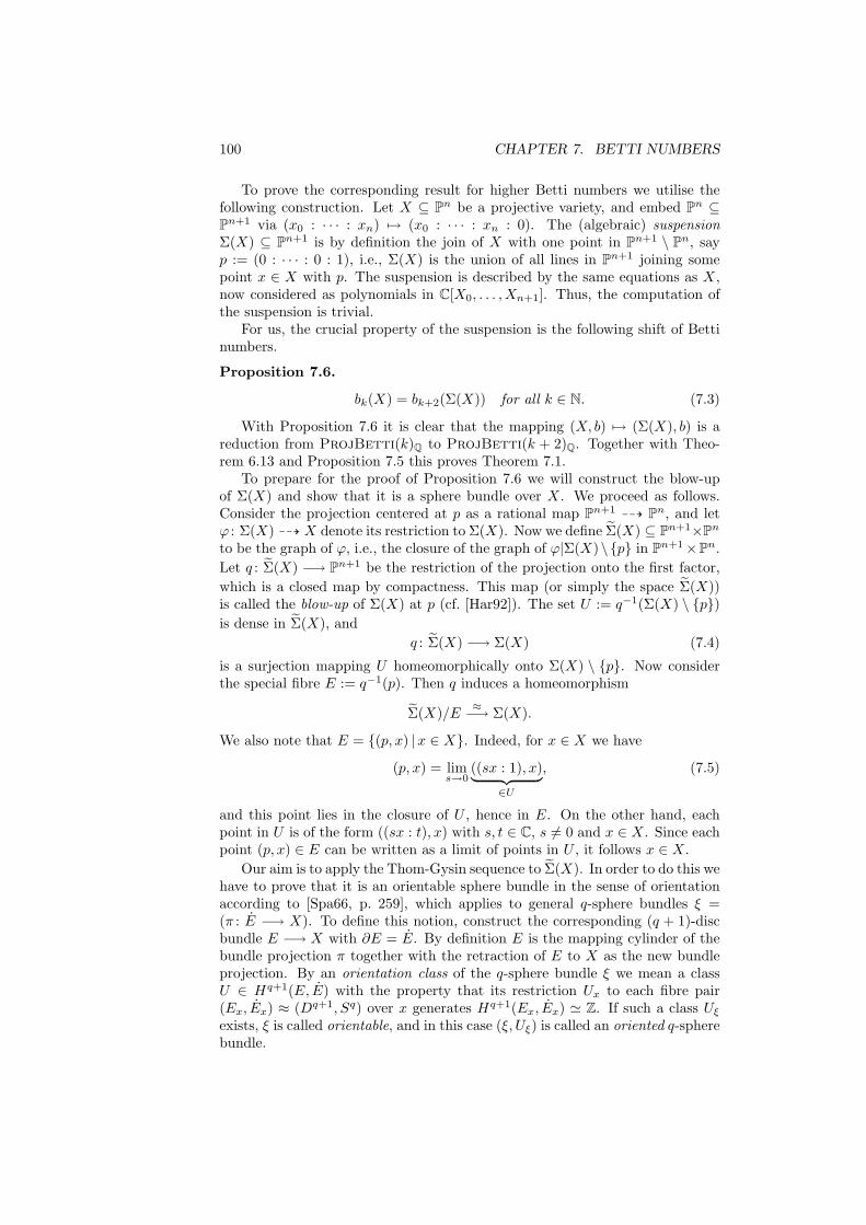
100 CHAPTER 7. BETTI NUMBERS
To prove the corresponding result for higher Betti numbers we utilise thefollowing construction. Let X ⊆ Pn be a projective variety, and embed Pn ⊆Pn+1 via (x0 : · · · : xn) 7→ (x0 : · · · : xn : 0). The (algebraic) suspensionΣ(X) ⊆ Pn+1 is by definition the join of X with one point in Pn+1 \ Pn, sayp := (0 : · · · : 0 : 1), i.e., Σ(X) is the union of all lines in Pn+1 joining somepoint x ∈ X with p. The suspension is described by the same equations as X,now considered as polynomials in C[X0, . . . , Xn+1]. Thus, the computation ofthe suspension is trivial.
For us, the crucial property of the suspension is the following shift of Bettinumbers.
Proposition 7.6.
bk(X) = bk+2(Σ(X)) for all k ∈ N. (7.3)
With Proposition 7.6 it is clear that the mapping (X, b) 7→ (Σ(X), b) is areduction from ProjBetti(k)Q to ProjBetti(k + 2)Q. Together with Theo-rem 6.13 and Proposition 7.5 this proves Theorem 7.1.
To prepare for the proof of Proposition 7.6 we will construct the blow-upof Σ(X) and show that it is a sphere bundle over X. We proceed as follows.Consider the projection centered at p as a rational map Pn+1 99K Pn, and letϕ : Σ(X) 99K X denote its restriction to Σ(X). Now we define Σ(X) ⊆ Pn+1×Pn
to be the graph of ϕ, i.e., the closure of the graph of ϕ|Σ(X)\p in Pn+1×Pn.Let q : Σ(X) −→ Pn+1 be the restriction of the projection onto the first factor,which is a closed map by compactness. This map (or simply the space Σ(X))is called the blow-up of Σ(X) at p (cf. [Har92]). The set U := q−1(Σ(X) \ p)is dense in Σ(X), and
q : Σ(X) −→ Σ(X) (7.4)
is a surjection mapping U homeomorphically onto Σ(X) \ p. Now considerthe special fibre E := q−1(p). Then q induces a homeomorphism
Σ(X)/E ≈−→ Σ(X).
We also note that E = (p, x) |x ∈ X. Indeed, for x ∈ X we have
(p, x) = lims→0
((sx : 1), x)︸ ︷︷ ︸∈U
, (7.5)
and this point lies in the closure of U , hence in E. On the other hand, eachpoint in U is of the form ((sx : t), x) with s, t ∈ C, s 6= 0 and x ∈ X. Since eachpoint (p, x) ∈ E can be written as a limit of points in U , it follows x ∈ X.
Our aim is to apply the Thom-Gysin sequence to Σ(X). In order to do this wehave to prove that it is an orientable sphere bundle in the sense of orientationaccording to [Spa66, p. 259], which applies to general q-sphere bundles ξ =(π : E −→ X). To define this notion, construct the corresponding (q + 1)-discbundle E −→ X with ∂E = E. By definition E is the mapping cylinder of thebundle projection π together with the retraction of E to X as the new bundleprojection. By an orientation class of the q-sphere bundle ξ we mean a classU ∈ Hq+1(E, E) with the property that its restriction Ux to each fibre pair(Ex, Ex) ≈ (Dq+1, Sq) over x generates Hq+1(Ex, Ex) ' Z. If such a class Uξ
exists, ξ is called orientable, and in this case (ξ, Uξ) is called an oriented q-spherebundle.

7.2. THE PROJECTIVE CASE 101
Lemma 7.7. Let ξ = (π : E −→ X) be an oriented q-sphere bundle, and Y ⊆ Xa subspace. Then π−1(Y ) −→ Y is also an orientable q-sphere bundle.
Proof. Let F := π−1(Y ), and F −→ Y be the corresponding q+1-disc bundle.Then the claim follows immediately from the fact, that the diagram
(Ex, Ex) → (E, E)‖ ↑
(Fx, Fx) → (F, F )
commutes for each x ∈ Y . 2
Lemma 7.8. The space Σ(X) is an orientable 2-sphere bundle over X.
Proof. Define π : Σ(X) −→ X to be the restriction of the projection pr2 : Pn+1×Pn −→ Pn onto the second factor.
To show that Σ(X) is locally trivial we use coordinates X0, . . . , Xn for Pn
and Z0, . . . , Zn+1 for Pn+1. Set Ui := X ∩ Xi 6= 0 ⊆ X ⊆ Pn and Vi :=π−1(Ui) for 0 ≤ i ≤ n. Then Vi = Σ(X) ∩ (Pn+1 × Xi 6= 0). Now define themaps
ϕi : Vi −→ Ui × P1, (z, x) 7→ (x, (zi : zn+1)), (7.6)
as well asψi : Ui × P1 −→ Vi, (x, (s : t)) 7→ ((sx : txi), x).
One easily checks that these maps are inverse to each other, hence ϕi is ahomeomorphism.
It remains to show that Σ(X) is orientable. Denote by D(X) −→ X the3-disc bundle corresponding to Σ(X). To prove the existence of an orientationclass, we use the embedding of X in the smooth complex manifold Pn, i.e., weconsider the diagram
(D(X), Σ(X)) ⊆ (D(Pn), Σ(Pn))↓ ↓X ⊆ Pn,
where the spaces on the right are smooth, hence orientable (as manifolds). Thenit is well-known that there exists the Thom class τ ∈ H3(D(Pn), Σ(Pn)) [Bre97,p. 368]. Since Pn is also connected, it follows from Corollary 11.6 of [Bre97,p. 370] that the restriction of τ to the fibre (D(Pn)x, Σ(Pn)x) of each pointx ∈ X is a generator. Hence the Thom class serves as an orientation class forΣ(Pn) in the above sense. It follows from Lemma 7.7 that Σ(X) −→ X is alsoorientable. 2
Proof of Proposition 7.6. Because of Lemma 7.8 we can apply the Thom-Gysinsequence (Theorem 11 from Section 5.7 of [Spa66, p. 260]) to the orientable 2-sphere bundle Σ(X) −→ X and get the exact sequence
· · · −→ Hk(X)ρ−→ Hk+2(Σ(X)) π∗−→ Hk+2(X) Ψ−→ Hk−1(X) −→ · · ·

102 CHAPTER 7. BETTI NUMBERS
The embedding i : X −→ Σ(X), x 7→ (p, x) satisfies π i = idX , hence π∗ i∗ =idH∗(X), thus π∗ is surjective. Then Ψ is the zero map, hence ρ is injective, andwe get the short exact sequence
0 −→ Hk(X) −→ Hk+2(Σ(X)) −→ Hk+2(X) −→ 0, (7.7)
which splits by i∗. It follows
Hk+2(Σ(X)) = Hk+2(X)⊕Hk(X) for k ∈ Z. (7.8)
To compute the homology of Σ(X) recall that it is homeomorphic to thequotient space Σ(X)/E. We want to apply Theorem 2.13 from [Hat02, p. 114],where we need the following technical condition.
Claim E = i(X) is a deformation retract of a neighbourhood in Σ(X).LetD ⊆ P1 be an open disc around (0 : 1). Define D :=
⋃ni=0 ϕ
−1i (Ui×D), where
the ϕi are the trivialisations defined in (7.6). Then D is an open neighbourhoodof E, and for all (z, x) ∈ D we have zn+1 6= 0. Now define
r : D −→ E, (z, x) 7→ (p, x).
Then r i = idE , thus r is a retraction. To show that r is homotopic to theidentity on D, define
H : [0, 1]× D −→ D, Ht(z, x) := ((tz0 : · · · : tzn : zn+1), x).
Then H is continuous, and we have H0(z, x) = ((0 : zn+1), x) = (p, x) = r(z, x),as well as H1(z, x) = (z, x) for all (z, x) ∈ D. Thus, the claim is proved.
Now we can apply Theorem 2.13 from [Hat02, p. 114], and get the followingexact sequence.
· · · −→ Hk+2(X) i∗−→ Hk+2(Σ(X))q∗−→ Hk+2(Σ(X)) ∂−→ Hk+1(X) −→ · · ·
Here q : Σ(X) −→ Σ(X) is the projection (7.4). The above sequence is originallyformulated for the reduced homology, but we restrict to the case k ≥ 0.
Now we use (7.8) and deduce from (7.7), that ker q∗ = im i∗ = Hk+2(X)via the isomorphism (7.8). Hence, q∗ induces an injective map Hk(X) −→Hk+2(Σ(X)). Since i∗ is injective, we have 0 = ker i∗ = im ∂, hence ker ∂ =Hk+2(Σ(X)) = im q∗, thus q∗ is surjective. It follows
Hk(X) = Hk+2(Σ(X)) for k ≥ 0,
completing the proof of Proposition 7.6. 2

Part III
Fixing Parameters
103


Chapter 8
Counting IrreducibleFactors
In this part we study the complexity of counting irreducible components forfixed input parameters like the number of variables, the number of equations,or their maximal degree. We focus here on the number of equations, which turnsout to be crucial. When input parameters are fixed, then the choice of the inputdata structure matters. We therefore add superscripts to specify the encodingof the input polynomials. We first discuss the case of a single equation. Asbefore k denotes a field of characteristic zero.
#IFk (Counting absolutely irreducible factors) Given a polynomial f ∈k[X1, . . . , Xn], compute the number of its pairwise coprime absolutely irre-ducible factors.
We will show
Theorem 8.1. We have
1. #IF(dense)k ∈ FNC2
k for each field k of characteristic zero,
2. #IF(dense)Q ∈ FNC2.
As described in the introduction, it was shown in [BCGW93] that #IF(dense)Q
lies in FNC.Note that Theorem 4.1 implies that #IF
(slp)Q ∈ FPSPACE. With regard to
the optimality of this statement, we know even less than for the problem #ICQ(cf. Proposition 4.2). The following lower bound is implied by [Pla77]. Here afunction f : 0, 1∞ → 0, 1∞ is said to be C-hard for a decisional complexityclass C iff its graph Γf = (x, f(x)) |x ∈ 0, 1∞ is C-hard.
Proposition 8.2. The problem #IF(slp)Q is coNP-hard with respect to polyno-
mial time many-one reductions.
Proof. In [Pla77] it is shown that the following problem is coNP-hard (withrespect to polynomial time many-one reductions).
105

106 CHAPTER 8. COUNTING IRREDUCIBLE FACTORS
Given univariate polynomials f1, . . . , fr ∈ Z[X] in sparse representation andN ∈ N in binary, decide whether
∏i fi has exactly N roots (counted without
multiplicities).
This problem is easily reducible to #IF(slp)Q . Indeed, given sparse polynomi-
als f1, . . . , fr ∈ Z[X], one can easily obtain slps computing the fi. From theseone easily computes an slp for g :=
∏i fi, and g has N roots iff (g,N) lies in
the graph of #IF(slp)Q . 2
Open question. Is #IF(slp)Q #P-hard?
Now we come to the proof of Theorem 8.1. As mentioned in the introductionGao [Gao03] has proposed a partial differential equation, whose solution spacehas a basis corresponding to the absolutely irreducible factors of a bivariatepolynomial. We show that this solution space is the first de Rham cohomologyof the hypersurface complement defined by the polynomial. From this charac-terisation we construct an efficient parallel algorithm for computing the numberof factors. Gao’s idea goes back to [Rup86], who formulated his results in thelanguage of differential forms. In our proof we will closely follow Ruppert’sapproach.
8.1 Cohomology of a Hypersurface Complement
For the characterisation of the factors of a polynomial f we will use the algebraicde Rham cohomology of the hypersurface complement defined by f . Recall thatin §1.2.1 we have introduced Kahler differentials. Recall also that k denotes afield of characteristic zero, and K := k.
For f ∈ k[X] we denote by Anf := An \ Z(f) the complement of the zero set
of f . The ring of regular functions on Anf is given by the localisation K[X]f
of the polynomial ring K[X] at the multiplicatively closed subset consisting ofpowers of f . We consider the de Rham complex of K[X]f over K, which is
Ω•K[X]f /K : 0 −→ K[X]fd0
−→ Ω1K[X]f /K
d1
−→ Ω2K[X]f /K
d2
−→ · · · .
The first algebraic de Rham cohomology H1(Anf ) of An
f is defined as the firstcohomology vector space of the de Rham complex Ω•K[X]f /K , i.e.,
H1(Anf ) = ker d1/im d0.
We will prove that H1(Anf ) has a basis consisting of “logarithmic differen-
tials”, by which we mean forms dff with f ∈ K[X]. First note that logarithmic
differentials are closed, as
d(
dff
)= d
(1f
df)
= d(
1f
)∧ df = − 1
f2df ∧ df = 0
for all f ∈ K[X]. Another nice feature of logarithmic differentials is that theybehave additively on products, i.e.,
d(fg)fg
=dff
+dgg
for all f, g ∈ K[X], (8.1)

8.2. STRUCTURE THEOREM FOR CLOSED 1-FORMS 107
which follows immediately from Leibnitz’ rule.The following is a refinement of a structure theorem for closed 1-forms in
ΩK(X1,X2)/K due to Ruppert [Rup86]. Its usefulness for algorithmic purposeswas first discovered by Gao [Gao03].
Theorem 8.3. Let f =∏s
i=1 feii be the factorisation of f ∈ k[X] into pairwise
coprime absolutely irreducible polynomials. Thendf1f1
, . . . ,dfs
fs
induce a basis of H1(Anf ). In particular, the dimension of H1(An
f ) equals thenumber of absolutely irreducible factors of f .
Example 8.4. In the following examples we freely use that over K := C the alge-braic de Rham cohomology of An
f coincides with singular cohomology [Gro66].
1. Let f := X ∈ C[X], i.e., A1X = C× ' S1. Then H1(A1
X) = CdXX .
2. Let f := X1 · · ·Xn ∈ C[X1, . . . , Xn], i.e., Anf = (C×)n. Then the Kunneth
Theorem implies the stronger statement
Hk(Anf ) =
⊕i1<···<ik
CdXi1
Xi1
∧ · · · ∧ dXik
Xik
for 0 ≤ k ≤ n.
3. The previous example can be generalised to complements of hyperplanearrangements (cf. [Bri73, OS80, JR91]). Let V =
⋃Ni=1Hi be a hyperplane
arrangement, where Hi = Z(αi) with linear forms αi ∈ (Cn)∗. ThenAn \ V = An
f with f =∏
i αi. It is known that the whole cohomologyring H∗(An
f ) is generated by the forms dαi
αi, 1 ≤ i ≤ N . Note that in
general there are more relations than in the previous example. One hasone relation for each linearly dependent subset of the αi (cf. [OS80, JR91]).
8.2 Structure Theorem for Closed 1-Forms
In this subsection we prove Ruppert’s structure theorem for closed 1-forms inΩK(X)/K [Rup86]. Recall that K is algebraically closed and has characteristiczero. We will need the following technical lemma.
Let L := K(X), and L an algebraic closure of L. Since L is a separablealgebraic extension of L (as L has characteristic zero), it follows from [ZS58,§17, Corollary 2’, p. 125] that the partial derivations ∂
∂Xi: L → L, 1 ≤ i ≤ n,
can be uniquely extended to derivations (which we denote with ∂∂Xi
again) of L.
Lemma 8.5. If α ∈ L satisfies ∂α∂Xi
= 0 for all 1 ≤ i ≤ n, then α ∈ K.
Proof. Let α ∈ L. By multiplying with a suitable element of K[X], we canassume that the minimal polynomial T ∈ L[Y ] of α is an element of K[X,Y ].From T (X1, . . . , Xn, α) = 0 we obtain
0 =∂
∂Xi
(T (X1, . . . , Xn, α)
)=
∂T
∂Xi(X1, . . . , Xn, α) +
∂T
∂Y(X1, . . . , Xn, α)
∂α
∂Xi
for any 1 ≤ i ≤ n. The assumption ∂α∂Xi
= 0 implies that ∂T∂Xi
annihilates α,hence T | ∂T
∂Xi. Since degY
∂T∂Xi≤ degY T , it follows ∂T
∂Xi= 0. As this holds for
all 1 ≤ i ≤ n, we have T ∈ K[Y ], thus α ∈ K, since K is algebraically closed. 2

108 CHAPTER 8. COUNTING IRREDUCIBLE FACTORS
Theorem 8.6 (Ruppert). For each differential form ω ∈ ΩK(X)/K with dω =0 there exist polynomials h1, . . . , hm, g, h ∈ K[X] and scalars λ1, . . . , λm ∈ Ksuch that
ω =m∑
i=1
λidhi
hi+ d( gh
). (8.2)
Remark 8.7. As noted above each ω of the form (8.2) is closed. It followsfrom (8.1) that in (8.2) we can assume the hi to be irreducible and pairwisecoprime.
Proof. We prove the theorem by induction on n. In the case n = 1 eachform ω = fdX with f ∈ K(X) is trivially closed since Ω2
K(X)/K = 0. To provethat ω can be written in the form (8.2), decompose f into partial fractions
f =m∑
i=1
ki∑j=1
aij
(X − ci)j+ b,
where aij , ci ∈ K and b ∈ K[X]. Now let c ∈ K[X] with c′ = b, where ′ denotesderivation. Also the quotients aij
(X−ci)j for j > 1 can be integrated, so set
Φ :=m∑
i=1
∑j>1
11− j
· aij
(X − ci)j−1+ c ∈ K(X).
With λi := ai1 and hi := X − ci it follows
f =m∑
i=1
ai1
X − ci+
m∑i=1
∑j>1
aij
(X − ci)j+ b =
m∑i=1
λih′ihi
+ dΦ′,
from which (8.2) follows.Let the closed 1-form ω be given in the form ω = 1
f
∑` g`dX` with g`, f ∈
K[X]. Then the closedness relation dω = 0 is equivalent to
∂
∂X`
(g`′
f
)=
∂
∂X`′
(g`
f
)for 1 ≤ `′ < ` ≤ n. (8.3)
Now we consider multivariate polynomials in K[X] as univariate polyno-mials in L[X1], where L := K(X2, . . . , Xn) is the fraction field in all but oneindeterminate. Let F ⊆ L be a splitting field of f ∈ L[X1]. Then there existu ∈ L× and pairwise distinct c1, . . . , cm ∈ F with f = u
∏mi=1(X1 − ci)ki . Now
we develop the rational coefficients from (8.3) into partial fractions
g`
f=
m∑i=1
ki∑j=1
a`ij
(X1 − ci)j+ b` for all 1 ≤ ` ≤ n, (8.4)
where a`ij ∈ F and b` ∈ F [X1].
According to the remarks preceding Lemma 8.5 we have the partial deriva-tions ∂
∂Xi: F [X1]→ F [X1] for 1 < i ≤ n, which map F into itself and the usual
8.2. STRUCTURE THEOREM FOR CLOSED 1-FORMS 109
∂∂X1
: F [X1]→ F [X1], which vanishes on F . Applying these to (8.4) yields
∂
∂X`
(g1f
)=
m∑i=1
ki∑j=1
(∂a1
ij
∂X`· 1(X1 − ci)j
+ja1
ij
(X1 − ci)j+1· ∂ci∂X`
)+∂b1
∂X`
=m∑
i=1
∂a1i1
∂X`· 1X1 − ci
+ki−1∑j=1
(∂a1
i,j+1
∂X`+ ja1
ij
∂ci∂X`
)· 1(X1 − ci)j+1
+kia
1i,ki
(X1 − ci)ki+1· ∂ci∂X`
)+∂b1
∂X`for all 1 < ` ≤ n and
∂
∂X1
(g`
f
)=−
m∑i=1
ki∑j=1
ja`ij
(X1 − ci)j+1+
∂b`
∂X1for all 1 < ` ≤ n.
Using (8.3) for `′ = 1 and the uniqueness of the partial fraction decompositionit follows
∂a1i1
∂X`= 0,
∂a1i,j+1
∂X`+ ja1
ij
∂ci∂X`
= −ja`ij (8.5)
for all ` > 1. By Lemma 8.5 it follows a1i1 ∈ K for all 1 ≤ i ≤ m. Analogously,
using (8.3) for general `′ < ` we obtain
∂b`′
∂X`=
∂b`
∂X`′for all 1 ≤ `′ < ` ≤ n. (8.6)
Hence the form∑
` b`dX` is closed.
By applying automorphisms of F over L to (8.4) and using the uniquenessof the partial fractions it follows
ci, ci′ conjugate over K ⇒ a`ij , a
`i′j conjugate over K (8.7)
for all i, i′, j, `. In particular, since a1i1, a
1i′1 ∈ K, they must coincide. From the
same argument we conclude b` ∈ L[X1].Thus there exists c ∈ L[X1] with ∂c
∂X1= b1. Since ∂
∂X1(b`− ∂c
∂X`) = 0 by (8.6),
we have b` − ∂c∂X`∈ L for all ` > 1, hence
η :=n∑
`=1
(b` − ∂c
∂X`
)dX` =
n∑`=2
(b` − ∂c
∂X`
)dX` ∈ ΩL/K .
From (8.6) we conclude that η =∑
` b`dX` − dc is closed. From the induction
hypothesis applied to η we obtain νj ∈ K, fj ∈ K[X2, . . . , Xn] for 1 ≤ j ≤ q,and r ∈ K(X2, . . . , Xn) with
η =q∑
j=1
νjdfj
fj+ dr. (8.8)
Now as in the univariate case we want to integrate as many terms as possiblein the partial fraction decomposition of g1
f with respect to X1, i.e., we want towrite
g1f
=m∑
i=1
a1i1
X1 − ci+
∂Φ∂X1
. (8.9)

110 CHAPTER 8. COUNTING IRREDUCIBLE FACTORS
This works analogously with
Φ :=m∑
i=1
ki∑j=2
11− j
·a1
ij
(X1 − ci)j−1+ c,
as one easily checks using (8.4). By applying all automorphisms of F over Lto Φ and using (8.7) we see that Φ is a rational function in K(X). Furthermore,
m∑i=1
−a1i1
X1 − ci∂ci∂X`
+∂Φ∂X`
+ b` − ∂c
∂X`(8.10)
=m∑
i=1
−a1i1
X1 − ci∂ci∂X`
+ki∑
j=2
( −a1ij
(X1 − ci)j
∂ci∂X`
+1
1− j
∂a1ij
∂X`
(X1 − ci)j−1
)+ b`
=m∑
i=1
ki∑j=1
(−a1
ij
∂ci∂X`
− 1j·∂a1
i,j+1
∂X`
)(X1 − ci)−j + b`
(8.5)=
g`
f
for all ` > 1.On the other hand, let J ⊆ 1, . . . ,m be the index set corresponding to
some conjugacy class of the ci and set uJ :=∏
i∈J(X1 − ci) ∈ K(X). Then
1uJ
∂uJ
∂X`=∑i∈J
−1X1 − ci
∂ci∂X`
for ` > 1.
Since µJ := a1i1 = a1
i′1 for all i, i′ ∈ J by (8.7), the first sum in (8.10) splits intothe sum of the terms µJ
1uJ
∂uJ
∂X`over all conjugacy classes J . Hence, using (8.9),
ω =n∑
`=1
g`
fdX` =
∑J
µJduJ
uJ+ dΦ + η.
Using (8.8) it follows
ω =∑
J
µJduJ
uJ+
q∑j=1
νjdfj
fj+ dr + dΦ,
which is of the desired form. 2
8.3 Proof of Theorem 8.3
We introduce a notation for divisibility of differential forms by polynomials. Forf ∈ K[X] and ω ∈ ΩK[X]/K we will write f |ω iff there exists η ∈ ΩK[X]/K withω = fη. Equivalenty, f |ω iff f |gi for all 1 ≤ i ≤ n, where ω =
∑i gidXi. We
will frequently use
Lemma 8.8. Let f, g ∈ K[X] with f |gdf . Then each irreducible factor of fdivides g.

8.3. PROOF OF THEOREM 8.3 111
Proof. Let h be an irreducible factor of f with multiplicity e ∈ N, i.e., thereexists h with heh = f and h - h. Then
gdf = g(ehhe−1dh+ hedh).
From f |gdf it follows he|eghhe−1dh. Since h - h, this implies h|gdh. This meansh|g ∂h
∂Xifor all i, from which we conclude h|g. 2
Proof of Theorem 8.3. We have already checked that the forms dfi
fiindeed
induce elements of the cohomology, i.e., they are closed.Then we show that the dfi
fiare linearly independent. Let
∑i λi
dfi
fi= 0 with
λ1, . . . , λr ∈ K. Then for each j we have
fj |
(∏`
f`
)∑i
λidfi
fi, hence fj |λj
∏` f`
fjdfj ,
and by Lemma 8.8 fj |λj
∏` 6=j f`, thus λj = 0.
Now we prove that these forms generate the cohomology. Let
ω =1f `
n∑i=1
gidXi ∈ ΩK[X]f /K with gi ∈ K[X]
be a closed 1-form. We can assume ` > 0, since otherwise ω would be a closed1-form with polynomial coefficients, which is exact.
By Theorem 8.6 there exist h1, . . . , hm, g, h ∈ K[X] and λ1, . . . , λm ∈ K×
such that
ω =1f `
n∑i=1
gidXi =m∑
j=1
λjdhj
hj+ d( gh
), (8.11)
where we can assume the hj to be irreducible and pairwise coprime accordingto Remark 8.7, also assume g and h coprime. Our aim is to prove that
1. each hj is one of the fi,
2. each irreducible factor of h is one of the fi
The second claim means that h divides some power of f , hence g/h ∈ K[X]f .Thus the decomposition (8.11) yields the representation of ω as a linear combi-nation of the dfi
fimodulo an exact form, and we are done.
Set H :=∏
j hj and multiply (8.11) with f `Hh2 to obtain
Hh2n∑
i=1
gidXi = f `h2m∑
j=1
λjH
hjdhj + f `H(hdg − gdh). (8.12)
Since each hj divides H, it follows hj |f `h2λjHhj
dhj , hence hj |f `h2λjHhj
byLemma 8.8. Since λj 6= 0, hj is irreducible, and hj - H/hj , we conclude
hj |fh for all 1 ≤ j ≤ m. (8.13)
On the other hand, (8.12) implies that h|f `Hgdh, and by Lemma 8.8 we have
p irreducible factor of h ⇒ p|fH, (8.14)

112 CHAPTER 8. COUNTING IRREDUCIBLE FACTORS
since g and h are coprime.Note that by (8.13) the second of the above claims implies the first, so we
prove the second. Let p be an irreducible factor of h with multiplicity e > 0,and write h = peu, where p - u. Then
d( gh
)=
dgh− e g
hpdp− g
hudu.
Multiplication of (8.11) with G := f`Hh2
pe = f `Hhu yields
Hhu∑
i
gidXi = f `hu∑
j
λjH
hjdhj + f `Hudg − ef
`H
pugdp− f `Hgdu.
By (8.14) this is a form with polynomial coefficients. Also by (8.14) it fol-lows that p|e f`H
p ugdp, hence by Lemma 8.8 p| f`Hp , thus p2|f `H, and since H
is squarefree, it follows p|f . Hence we haved shown claim 2, which completes theproof. 2
8.4 Characterising Exact Forms
The implications of Theorem 8.3 are twofold. First it shows that the dimensionof H1(An
f ) is the number of irreducible factors of the polynomial f . But since
dfi
fi=
1f
n∑j=1
f
fi
∂fi
∂XjdXj ,
it also shows that this space has a basis induced by forms with denominator fand numerators of degree < d := deg f . Hence, all elements of the cohomologyhave representatives of this form.
Now one might hope that it were possible to ignore exact forms with thehelp of some maybe more restricted degree condition. This means that thede Rham cohomology would be isomorphic to the space of closed 1-forms withdenominator f and numerators satisfying this degree condition. Note that eachcohomology class in H1(An
f ) is represented by a form ω = 1f
∑i gidXi satisfying
the degree condition
degXjgi ≤ degXj
f for j 6= i, degXigi < degXi
f. (8.15)
This condition was utilised by Gao to make the representatives unique. Inparticular he proved that under the condition gcd(f, ∂f
∂X1) = 1 the space of
closed 1-forms satisfying (8.15) is isomorphic to H1(Anf ). However, this is not
true in the general case, as the following example shows.
Example 8.9. Let f = g2 with irreducible g ∈ K[X]. Then the closed form
ω :=dgg2
=1f
n∑i=1
∂g
∂XidXi
satisfies (8.15). But as ω = d(− 1
g
)is exact, its cohomology class is zero.

8.4. CHARACTERISING EXACT FORMS 113
Hence we also have to consider the exact forms. Our aim now is to char-acterise the subspace of exact forms with denominator f and numerators ofdegree < d. For that purpose we show that each such form is the differential ofa rational function g/f with deg g < d+ 1.
Lemma 8.10. Let f, g, g1, . . . , gn ∈ K[X], and ` ∈ N with f - g and f - gi forsome i such that
d(g
f `
)=
1f
n∑i=1
gidXi.
Then ` = 1.
Proof. We have
d(g
f `
)=fdg − `gdf
f `+1,
hence by assumption
fdg − `gdf = f `∑
i
gidXi. (8.16)
If ` = 0, then (8.16) implies f |gi for all i, which contradicts the assumption.Hence ` ≥ 1.
Let f =∏s
i=1 feii be the factorisation of f . Since by (8.16) we have f |gdf ,
Lemma 8.8 implies fi|g for all i. Then (8.16) implies with (8.1)
f `|(fdg − `gdf) = fdg − `gf∑
i
eidfi
fi= f
(dg − `
∑i
eig
fidfi
),
hencef `−1|
(dg − `
∑i
eig
fidfi
).
Now h := gcd(f, g) factorises as h =∏s
i=1 fµi
i with 1 ≤ µi ≤ ei. Writing g = huwith some u we conclude
f `−1|(udh+ hdu− `∑
i
eig
fidfi) = hdu+
∑i
(µi − `ei)uh
fidfi. (8.17)
Now assume ` ≥ 2. Then µj−`ej ≤ −ej < 0 for all j, and fµj
j |u hfj
dfj by (8.17).
Hence fj |u by Lemma 8.8, thus fµj+1j |g, which implies µj = ej . Since this holds
for all j, it follows f |g, which contradicts our assumption. Therefore ` = 1. 2
Lemma 8.11. Let f, g, g1, . . . , gn ∈ K[X] with deg gi < d := deg f for all isuch that
d(g
f
)=
1f
n∑i=1
gidXi.
Then deg g < d+ 1.

114 CHAPTER 8. COUNTING IRREDUCIBLE FACTORS
Proof. As in (8.16) we have fdg − gdf = f∑
i gidXi. Now let e := deg g andwrite g = g0 + · · ·+ge and f = f0 + · · ·+fd with gi, f i homogeneous of degree i.Then
f∑
i
gidXi =d∑
i=0
e∑j=0
(f idgj − gjdf i) =d+e∑`=0
∑i+j=`
(f idgj − gjdf i). (8.18)
In the trivial case ge
fd ∈ K we have e = d < d+ 1, so assume ge
fd /∈ K. Then
d(ge
fd
)=fddge − gedfd
(fd)26= 0.
It follows that the form (8.18) contains a coefficient of degree d + e − 1, thusd+ e− 1 ≤ d+ maxi deg gi < 2d, hence e < d+ 1. 2
8.5 Proof of Theorem 8.1
Let f ∈ k[X] be of degree d. Consider the finite dimensional vector spaces
Ω :=
1f
∑i
gidXi ∈ ΩK[X]f /K | deg gi < d for all i
,
Z :=ω ∈ Ω |dω = 0,
B :=ω ∈ Ω | ∃g ∈ K[X] with d
(g
f
)= ω
The linear map Z → ker d1 H1(An
f ) induces a map Z/B → H1(Anf ). This
map is surjective by Theorem 8.3 and injective by Lemmas 8.10 and 8.11, hence
H1(Anf ) ' Z/B.
Thus dimH1(Anf ) = dimZ − dimB.
For the form ω = 1f
∑i gidXi ∈ Ω the condition dω = 0 is equivalent to
f
(∂gi
∂Xj− ∂gj
∂Xi
)+ gj
∂f
∂Xi− gi
∂f
∂Xj= 0 for 1 ≤ i < j ≤ n. (8.19)
The equations (8.19) form a homogeneous linear system of equations over k inthe coefficients of the polynomials g1, . . . , gn. Its size is polynomial in
(d+n
n
),
hence by §1.5.1 one can compute dimZ in FNC2k.
Now consider the space B. For ω ∈ Ω as above and g ∈ K[X]≤d the condition
d(
gf
)= ω is equivalent to
f∂g
∂Xi− g ∂f
∂Xi− fgi = 0 for 1 ≤ i ≤ n. (8.20)
The equations (8.20) form a homogeneous linear system over k in the coefficientsof the polynomials g, g1, . . . , gn. Let
L := (g, g1, . . . , gn) ∈ K[X]≤d ×K[X]n≤d−1 | (8.20) holds

8.6. COUNTING IRREDUCIBLE COMPONENTS REVISITED 115
be its solution space. Consider the projection
π : L −→ K[X]n≤d−1, (g, g1, . . . , gn) 7→ (g1, . . . , gn).
By definition its image π(L) is isomorphic to B. Its kernel is the one-dimensionalspace
N :=
(g, 0, . . . , 0) |d(g
f
)= 0
= K(f, 0, . . . , 0),
thusB ' L/N,
hence dimB = dimL− 1. So it suffices to compute the dimension of L, whichis the solution space of the linear system (8.20), whose size is also polynomialin(d+n
n
). By §1.5.1 this proves #IF
(dense)k ∈ FNC2
k.The statement for the case k = Q follows from §1.5.1 by observing that the
linear systems (8.19) and (8.20) have coefficients of bitsize O(` log d), where ` isthe maximal bitsize of the coefficients of f . 2
8.6 Counting Irreducible Components Revisited
Our results about counting irreducible factors can be used for counting theirreducible components of a variety and yield a second proof of Theorem 4.1.This proof uses the Chow form associated to an equidimensional projectivevariety. We first recall its definition and basic properties. For further details werefer to [Sha77].
We identify the space of linear forms on Pn with Pn by associating to a pointu = (u0 : · · · : un) ∈ Pn the linear form L(u,X) := u0X0 + · · · + unXn up toa constant factor. A linear subspace L ⊆ Pn of codimension m + 1 is the zeroset of m+ 1 linearly independent linear forms L(ui, X) = ui0X0 + · · ·+ uinXn,0 ≤ i ≤ m. Now let V ⊆ Pn be an equidimensional projective variety ofdimension m. The intersection of V with a linear subspace of codimension m+1is almost always empty, and the set of such subspaces meeting V constitutes avariety. More precisely, consider the incidence variety
Γ := (x, u0, . . . , um) ∈ Pn × (Pn)m+1 |x ∈ V ∧ L(u0, x) = · · · = L(um, x) = 0
and the projection
π : Pn × (Pn)m+1 −→ (Pn)m+1, (x, u0, . . . , um) 7→ (u0, . . . , um).
Then in [Sha77] it is shown that π(Γ) ⊆ (Pn)m+1 is a hypersurface. Thus,introducing m+1 groups of new variables Ui = (Ui0, . . . , Uin), 0 ≤ i ≤ m, thereexists a unique (up to a scalar factor) squarefree polynomial FV ∈ k[U0, . . . , Um]defining π(Γ). This polynomial is called the Chow form associated to V . It ishomogeneous of degree deg V in each group Ui of variables and symmetric withrespect to permutations of the vectors Ui. Furthermore, to the decompositionV = V1 ∪ · · · ∪ Vs into irreducible components corresponds the factorisationFV = FV1 · · · FVs of the corresponding Chow form.
In [GH91a] it is proved that one can compute the Chow form of a projectivevariety in parallel polynomial time. Caniglia [Can90] considered an extended

116 CHAPTER 8. COUNTING IRREDUCIBLE FACTORS
notion of Chow forms of arbitrary unmixed ideals (not necessarily radicals),where the exponents of the primary components appear as multiplicities of thefactors in the Chow form. He showed that this Chow form can also be computedin parallel polynomial time for unmixed ideals. The state of the art algorithmfor computing the Chow form has been given in [JKSS04], where an slp forthe Chow form of a projective variety given by slps is computed in randomisedpolynomial time in the input size and the degree of the input system. All thesepapers show the following Theorem.
Theorem 8.12. Given homogeneous polynomials f1, . . . , fr ∈ k[X0, . . . , Xn]of degree at most d defining a projective variety V , one can compute for each0 ≤ m ≤ n the Chow form of the m-equidimensional component of V in paralleltime (n log(rd))O(1) and sequential time (rd)nO(1)
.
Proof of Theorem 4.1. 1. Let the projective variety V := Z(f1, . . . , fr) begiven by the homogeneous polynomials f1, . . . , fr ∈ k[X0, . . . , Xn], and denoteby Fm := FVm
for each 0 ≤ m ≤ n the Chow form of the m-equidimensionalcomponent Vm of V . According to Theorem 8.12 one can compute the Fm inparallel polynomial time. By Theorem 8.1 we can compute the number im ofirreducible factors of Fm in parallel polylogarithmic time in the size of Fm, thuswe can compute im in parallel polynomial time in the input size, even thoughthe size of Fm is exponential in general. As remarked above, the number ofirreducible components of V is i0 + · · · + in. Thus #ProjICk ∈ FPARk. Thestatement about the affine case follows from Proposition 4.3.
2. This follows from the transfer result Theorem 2.3. 2

Chapter 9
Fixed Number of Equations
We study the complexity of #ICk for a fixed number of equations in the powerfulslp encoding of polynomials together with a bound on their formal degrees inunary. As usual we understand slps to be division-free. In this chapter k denoteseither C or Q and K = C.
#IC(r)(d-slp)k Given a fixed number r of polynomials f1, . . . , fr ∈ k[X]
encoded as slps and an upper bound on their formal degrees in unary, computethe number of irreducible components of their zero set Z(f1, . . . , fr) ⊆ An.
#ProjIC(r)(d-slp)k Given a fixed number r of homogeneous polynomials
f1, . . . , fr ∈ k[X] encoded as slps and an upper bound on their formal degreesin unary, compute the number of irreducible components of their projective zeroset Z(f1, . . . , fr) ⊆ Pn.
Notice that in these problems the formal degree is part of the input andnot fixed. Our main results about these problems are stated in the followingtheorem. For the definition of the randomised parallel complexity class FRNCsee Definition 2.5.
Theorem 9.1. We have
1. #IC(r)(d-slp)C ,#ProjIC(r)(d-slp)
C ∈ FPC,
2. #IC(r)(d-slp)Q ,#ProjIC(r)(d-slp)
Q ∈ FRNC.
Theorem 9.1 follows with general principles from a fundamental generic par-simonious reduction of #ProjIC(r)(d-slp)
C to the case of a fixed dimension ofthe ambient space. In the next section we show how this works.
9.1 Proof of the Main Results
As an auxiliary problem we use #ProjIC(r)(d-slp)k restricted to a fixed dimen-
sion n of the projective ambient space. We denote this restricted version by#ProjIC(r, n)(d-slp)
k . The cornerstone of the proof of Theorem 9.1 is the fol-lowing proposition. Recall that ∗ denotes a generic parsimonious reduction(Definition 2.10).
117

118 CHAPTER 9. FIXED NUMBER OF EQUATIONS
Proposition 9.2. We have #ProjIC(r)(d-slp)C ∗ #ProjIC(r, r+1)(d-slp)
C viaa reduction map π such that πQ is computable in FNC.
Before proving this proposition, we show how it implies Theorem 9.1. Firstnote that by Remark 4.4 there is a Turing reduction from #IC(r)(d-slp)
C to#ProjIC(r+1)(d-slp)
C , hence it suffices to consider the projective case. Now weobserve that for a fixed ambient dimension we have already a parallel polylog-arithmic time algorithm.
Proposition 9.3. We have #ProjIC(r, n)(d-slp)C ∈ FNCC.
Proof. Given slps of length at most L and with formal degree at most d encod-ing the homogeneous polynomials f1, . . . , fr ∈ C[X], we compute their denserepresentation according to Proposition 1.27 in parallel time O(logL log dL +n2 log2 d) and sequential time (Ldn)O(1). Then we use Theorem 4.1 to computethe number of irreducible components of V in parallel time (n log d)O(1) andsequential time dnO(1)
. Since n is fixed and d is bounded by the input size, weobtain FNCC-algorithms. 2
Now by Theorem 2.11 the generic parsimonious reduction from Proposi-tion 9.2 yields a Turing reduction from #ProjIC(r)(d-slp)
C to #ProjIC(r, r +1)(d-slp)
C . Together with Proposition 9.3 this proves the first part of Theorem 9.1.Note that Theorem 2.11 is the point where we loose the good parallelisationproperties of our algorithms.
We prove the second part of Theorem 9.1 similarly as the first part withProposition 9.2. Although one can avoid randomisation by analysing the bitsizegrowth of the known algorithms, we can easily obtain the following result byone of our general transfer principles.
Proposition 9.4. We have #ProjIC(r, n)(d-slp)Q ∈ FRNC.
Proof. First note that the output size of #ProjIC(r, n)(d-slp)Q is logarithmic,
since the number of irreducible components of a projective variety in Pn isbounded by dn, where d is the maximal degree of the input polynomials (cf.Remark 1.7). Since a bound on d is part of the input and the ambient dimensionn is fixed, this quantity is polynomial in the input size.
We thus prove the more general statement, that for any function f : C∞ → Nwith logarithmic output size on binary inputs f ∈ FNCC implies fQ ∈ FRNC.More precisely, the assumption is |fQ(x)| = O(log |x|) for all x ∈ 0, 1∞.Recall from the beginning of §2.1 that fQ = γ f δ, where δ interprets pairs ofintegers as their quotients and γ encodes rational numbers as reduced fractionswritten in binary. Choose c > 0 with |fQ(x)| ≤ c log |x| for |x| 0, anddenote λ(n) := dc log ne. The key point of our assumption is that for an inputx ∈ 0, 1n there is only a polynomial number of candidates y ∈ 0, 1λ(n) forfQ(x). Note that for all x ∈ 0, 1n and y ∈ 0, 1λ(n)
fQ(x) = y ⇔ f δ(x) = δ(y). (9.1)
Given x and y, property (9.1) can be tested in NCC, since δ and f can becomputed in FNCC. We conclude from Theorem 2.8 that one can test (9.1) in

9.2. TRANSVERSALITY 119
FRNC. Note that such a test has a two-sided error, i.e., its result can be wrongin either case.
To compute fQ(x) on input x ∈ 0, 1n, we proceed as follows. For eachy ∈ 0, 1λ(n) (in parallel) test whether (9.1) holds. If all these tests are negative,output an arbitrary y. If there is at least one y with a positive test, output anarbitrary of these y.
Of course, when implementing this algorithm, we have to replace the arbi-trary choices by definite ones, e.g., we choose the first y (with positive test)in some fixed order. To show that this is indeed an FRNC-algorithm, we haveto analyse the error probability. Let 0 < q < 1 be such that the test (9.1)has error probability ε ≤ qn+λ(n) (note that the input for that test is (x, y)).Denote by yr the output of the algorithm, and by B the event that all tests arenegative. Then the failure probability of the algorithm is
P (yr 6= f(x)) = P (yr 6= f(x) ∧B) + P (yr 6= f(x) ∧B),
where we write B for the complement of B. We bound the first of these proba-bilities by
P (B) ≤ P (test for y = f(x) negative) ≤ ε.The second probability is bounded by the conditional probability
P (yr 6= f(x) |B) ≤ ε,
since this is exactly the failure probability of the test for yr. We conclue P (yr 6=f(x)) ≤ 2ε ≤ 2qn+λ(n). Since λ(n) ≥ c log n, we have 2qλ(n) ≤ 2nc log q ≤ 1 forn 0, hence the error probability of our algorithm is bounded by qn for n 0.This proves fQ ∈ FRNC. 2
With the help of Theorem 2.17 the generic reduction from Proposition 9.2yields #ProjIC(r)(d-slp)
Q R #ProjIC(r, r + 1)(d-slp)Q . Since FRNC is closed
under randomised parsimonious reductions (Lemma 2.15), this implies togetherwith Proposition 9.4 that #ProjIC(r)(d-slp)
Q ∈ FRNC. By Lemma 4.5 the reduc-
tion from #IC(r)(d-slp)Q to #ProjIC(r + 1)(d-slp)
Q is computable in FNC, hence
also #IC(r)(d-slp)Q ∈ FRNC.
The following sections are devoted to the proof of Proposition 9.2.
9.2 Transversality
For a lack of reference we give a detailed definition of transversality appropriatefor our purposes. It generalises the one of [Mum76, pp. 80-81] to reduciblevarieties. Note that we even allow varieties of mixed dimensions. Althougheverything in this section works for arbitrary algebraically closed coordinatefields, we work over C.
Recall that for two subspaces M,N of a finite dimensional vector space Lwe have dim(M ∩N) ≥ dimM + dimN − dimL. This statement is generalisedto varieties by the Dimension Theorem (cf. page 19).Definition 9.5.
1. Let M,N be two subspaces of a finite dimensional vector space L. We saythat M and N are transversal (in L) and write M t N iff
dim(M ∩N) = dimM + dimN − dimL.
120 CHAPTER 9. FIXED NUMBER OF EQUATIONS
2. Let V,W ⊆ Pn be projective varieties. We say that V and W are transver-sal in x ∈ V ∩W and write V tx W iff x is smooth in V and W , and TxVis transversal to TxW in TxPn.
3. Let V,W ⊆ Pn be a two varieties. We say that V and W are transversaland write V t W iff for almost all x ∈ V ∩W we have V tx W .
Note that V ∩W = ∅ implies V t W . We first show that if two varietiesintersect transversally in a point, then the intersection is smooth at that point,and the tangent space of the intersection is the intersection of their tangentspaces at that point.
Lemma 9.6. Let V,W ⊆ Pn be varieties. If V tx W holds in x ∈ V ∩W ,then x is smooth in V ∩W and Tx(V ∩W ) = TxV ∩ TxW .
Proof. First note that we have for all x ∈ V ∩W (no matter whether V and Ware transversal or not)
dimx(V ∩W ) ≥ dimx V + dimxW − n. (9.2)
Indeed, let Z ⊆ V and X ⊆W be irreducible components of maximal dimensionwith x ∈ Z and x ∈ W , i.e., dimx V = dimZ and dimxW = dimX. Then bythe Dimension Theorem (page 19)
dimx(V ∩W ) ≥ dimx(Z ∩X) ≥ dimZ + dimX − n = dimx V + dimxW − n.
Now let x ∈ V ∩W with V tx W . Since by definition x is smooth in V , wehave dimx V = dimTxV , and similarly for W . Then
dimx(V ∩W ) ≤ dimTx(V ∩W ) ≤ dim(TxV ∩ TxW )= dimTxV + dimTxW − n = dimx V + dimxW − n.
With (9.2) equality follows. This proves all claims of the Lemma. 2
Transversal varieties intersect properly.
Proposition 9.7. Let V,W ⊆ Pn be varieties with V t W . Then the intersec-tion is proper, i.e., for all x ∈ V ∩W we have
dimx(V ∩W ) = dimx V + dimxW − n. (9.3)
Proof. Note that by the proof of Lemma 9.6 the formula (9.3) holds in allpoints x ∈ V ∩W with V tx W . To show the formula for all points, recall thatthe function V −→ N, x 7→ dimx V is upper semi-continuus, i.e., for all α ∈ Rthe set x ∈ V | dimx V ≤ α is open in V .
Now let x ∈ V ∩ W be arbitrary. Let Z be an irreducible component ofV ∩W of maximal dimension with x ∈ Z, i.e., dimx(V ∩W ) = dimZ. By theupper semi-continuity, the sets UV := y ∈ V | dimy V ≤ dimx V and UW :=y ∈W | dimy W ≤ dimxW are open and non-empty, since x ∈ UV ∩UW . Bytransversality there exists an open dense subset U ⊆ V ∩W such that V ty Wfor all y ∈ U . By Lemma 9.6 we have U ∩ Z ⊆ Reg (Z). Furthermore U ∩ Z isopen in Z and non-empty. The sets UV ∩Z and UW ∩Z are also open in Z and

9.2. TRANSVERSALITY 121
contain x, hence U := U ∩ UV ∩ UW ∩ Z is a non-empty open subset of Z. Forall y ∈ U we have
dimx(V ∩W ) = dimZ ≤ dimy(V ∩W ) = dimy V + dimy W − n≤ dimx V + dimxW − n,
where in the last step we used y ∈ UV ∩ UW . With (9.2) this proves (9.3). 2
Let us gather some relationships between local and global transversalitystatements, which follow easily from Definition 9.5 and Proposition 9.7.
Lemma 9.8. Let V,W ⊆ Pn be varieties.
1. If V t W , then for all x ∈ V ∩W we have dimx V + dimxW ≥ n.
2. If V and W are equidimensional and transversal, then V ∩W is equidi-mensional of dimension dimV + dimW − n.
3. Let V =⋃
i Vi and W =⋃
j Wj be the irreducible decompositions of Vand W , respectively. Then
∀i, j Vi t Wj ⇒ V t W.
4. Let V and W be equidimensional and V =⋃
i Vi and W =⋃
j Wj be theirirreducible decompositions. Then
V t W ⇒ ∀i, j Vi t Wj .
5. Let V = V0 ∪ · · · ∪ Vn and W = W0 ∪ · · · ∪Wn be the equidimensionaldecompositions of V and W . Then
∀m,m′ Vm t Wm′ ⇒ V t W.
Proof.
1. By Proposition 9.7 we have dimx V + dimxW − n ≥ 0 in all points x ∈V ∩W .
2. Follows immedately from Proposition 9.7.
3. First assume W to be irreducible and let Vi t W for all i. Let Ui ⊆ Vi∩Wbe an open dense subset with Vi tx W for all x ∈ Ui. Then the Ui arepairwise disjoint, since Ui ⊆ Reg (Vi). Furthermore,
⋃i Ui is dense in
V ∩W . If x ∈ Ui, then Vi tx W implies V tx W .Now, if W is also reducible, and Vi t Wj for all i, j, fix j and concludefrom the first case that V t Wj . Again by the first case V t W .
4. Fix i, j. By Proposition 9.7 we have for x ∈ Vi ∩Wj
dimx(Vi ∩Wj) ≤ dimx(V ∩W ) = dimx V + dimxW − n= dimx Vi + dimxWj − n,
where in the last step we have used the equidimensionality of V and W .It follows that Vi∩Wj is equidimensional of the same dimension as V ∩W(use part 2). Hence each irreducible component of Vi∩Wj is a componentof V ∩W . Now let U ⊆ V ∩W be an open dense subset with V tx Wfor all x ∈ U . Then U meets each component of Vi ∩Wj and is thereforedense therein. It follows Vi t Wj .

122 CHAPTER 9. FIXED NUMBER OF EQUATIONS
5. Writing Vm =⋃
i Vmi and Wm =⋃
j Wmj for the irreducible decomposi-tions of Vm and Wm, respectively, we have
∀m,m′ Vm t Wm′ ⇒ ∀m,m′, i, j Vmi t Wm′j ⇒ V t W
by parts 3 and 4. 2
The converse of Part 3 of the above lemma does not hold in general, as thefollowing example shows.
Example 9.9. Let V = V1 ∪ V2 ⊆ P3 be the union of the plane V1 = Z(X2)and the parabola V2 = Z(X0X1 − X2
2 , X3), and L = Z(X1). Then V ∩ L =Z(X1, X2), where V ∩xL is satisfied in all points x of V ∩L except (1 : 0 : 0 : 0),hence V t L. But, of course, we don’t have V2 t L (cf. Figure 9.1).
Note also that V2 ∩ L is a proper intersection, but not transversal.
Figure 9.1: The plane L is transversal to V1 ∪ V2, but not to V2.
Remark 9.10. Let V ⊆ Pn be an irreducible variety of dimension m. It isknown [Mum76] that for s ≤ n−m almost all L ∈ Gs(Pn) satisfy L t V (whichin the case s < n −m is equivalent to L ∩ V = ∅). This statement generalisesto reducible varieties and arbitrary dimensions, which we will see later.
9.3 Explicit Genericity Condition for Bertini
The main idea in the proof of Proposition 9.2 is the Theorem of Bertini [Mum76,Corollary 4.18]. It says that an irreducible projective variety V of dimension mand a generic linear subspace L of codimension m − 1 meet transversally inan irreducible curve. This easily implies that if V is m-equidimensional, thenumber of irreducible components is preserved under intersections with generic

9.3. EXPLICIT GENERICITY CONDITION FOR BERTINI 123
linear subspaces of codimension m − 1. As our aim is to apply the conceptof generic parsimonious reductions (cf. §2.2), we want to identify an explicitcondition on L under which V ∩ L has the same number of components as V .It is not enough to require transversality, as the following example shows.
Example 9.11. Let V = Z(X0X3 −X21 ) ⊆ P3 be the cylinder over a parabola,
and consider the plane L = Z(X0−X3). Then V is irreducible and V t L, butV ∩ L = Z(X1 +X3, X0 −X3) ∪ Z(X1 −X3, X0 −X3) is reducible.
Figure 9.2: The plane L cuts V into two components.
To formulate our genericity condition, we introduce some notation. Re-call from §1.1.4 that we denote by Gs(Pn) the Grassmannian variety consistingof all linear subspaces of dimension s. Linear subspaces L ⊆ Pn are definedby linear forms α1, . . . , αn−s, which we identify with the row vectors given bytheir coefficients. We write the row vectors αi as a matrix α = (αij)
n−s,ni=1,j=0 ∈
C(n−s)×(n+1). We parametrise all linear subspaces of dimension ≥ s by suchmatrices α ∈ C(n−s)×(n+1), and write Lα for the linear subspace defined by α.
For Lβ ∈ Gs(Pn), β ∈ C(n−s)×(n+1), the projection centered at Lβ is definedby
pβ : Pn \ Lβ −→ Pn−s−1, x 7→ (β1(x) : · · · : βn−s(x)).
Although denoted by pLβin the literature, we denote the projection by pβ , since
this map clearly depends on the choice of β.Now let V be m-equidimensional and Lβ ∈ Gn−m−1(Pn) with Lβ ∩ V = ∅.
Let p : V → Pm be the restriction of pβ to V . We define the set of branchingvalues (cf. §1.1.3)
Bβ(V ) := y ∈ Pm | p is not smooth over y.
Note that Bβ(V ) depends on the choice of β, whereas the set p−1(Bβ(V )) does

124 CHAPTER 9. FIXED NUMBER OF EQUATIONS
not. It follows from the algebraic version of Sard’s Lemma (cf. [Mum76, Lemma3.7] or [Har92, Proposition 14.4]) that Bβ(V ) is a proper subvariety of Pm.
For the general case we fix a variety V , which is defined by r homogeneouspolynomials. Then the dimension of each irreducible component of V is boundedfrom below by n−r. Hence the decomposition into equidimensional componentsreads as V = Vn−r ∪ · · · ∪ Vn, where dimVm = m or Vm = ∅. Therefore weconsider linear subspaces L ⊆ Pn of dimension r + 1. Our genericity conditionfor L is
n∧m=n−r
(∃β ∈ C(m+1)×(n+1) ∃` ∈ G1(pβ(L)) : rkβ = m+ 1 ∧ Lβ ⊆ L ∧
Lβ ∩ Vm = ∅ ∧ ` t Bβ(Vm)). (9.4)
Note that dim pβ(L) ≥ 1. We denote condition (9.4) by BV (L). Before weproceed further, we show why V and L from Example 9.11 do not satisfy BV (L).Example 9.12. (continued) In the situation of Example 9.11 we have n = 3, Vis irreducible of dimension m = 2, hence M = Lβ according to formula (9.4)is a point in L \ V . One easily sees that for each such M the set of branchingvalues B := Bβ(V ) is the union of two lines meeting in some point of pβ(L).Furthermore, since dimL = 2, we have dim pβ(L) = 1. Thus, each line ` in pβ(L)coincides with pβ(L), so ` meets B in a singular point, hence not transversally.(cf. Figure 9.3).
The plane L′ := Z(X0 +X2 −X3) satisfies BV (L′) (cf. Figure 9.4).
Figure 9.3: The line pβ(L) meets B in a singular point.
Now we show that BV (L) implies that L meets V transversally.
Lemma 9.13. Let L be a linear subspace of dimension r+ 1 satisfying BV (L).Then L t V .

9.3. EXPLICIT GENERICITY CONDITION FOR BERTINI 125
Figure 9.4: For the plane L′ we have pβ(L′) t B.
Proof. By part 5 of Lemma 9.8 it is enough to prove that Vm t L for each m,so we can assume V to be m-equidimensional. Let M := Lβ be as in (9.4), andset p := pβ |V , L′ := pβ(L), B := Bβ(V ), and U := p−1(L′ \B). We show
1. V tx L for all x ∈ U , and
2. U is dense in p−1(L′) = V ∩ L.
1. By definition of B each x ∈ U is a smooth point of V , and the differentialdxp : TxV → Tp(x)Pm is an isomorphism. So dxp maps TxV ∩ TxL injectivelyinto Tp(x)L
′, hence dim(TxV ∩TxL) ≤ dimL′ = m+r+1−n. Since the oppositeinequality is trivial, equality follows.
2. Since there exists ` ⊆ L′ with ` t B, it follows that L′ ∩ B is a propersubvariety of L′, hence dim(B ∩L′) < dimL′. From the Noether NormalisationLemma in the form [Mum76, Corollary (2.29)] we conclude that p : V → Pm hasfinite fibres. Thus
dim p−1(B ∩ L′) = dim(B ∩ L′) < dimL′ = m+ r + 1− n ≤ dimZ
for each irreducible component Z of V ∩L. It follows that U∩Z = Z\p−1(B∩L′)is not empty. Hence U meets each irreducible component of V ∩ L, i.e., U isdense in V ∩ L.
By definition of transversality it follows L t V . 2
Next we have to prove that condition BV (L) is indeed generically fulfilled.
Lemma 9.14. Almost all L ∈ Gr+1(Pn) satisfy BV (L).

126 CHAPTER 9. FIXED NUMBER OF EQUATIONS
Proof. Since a finite intersection of dense subsets is dense, it is sufficient toprove that for each m ≥ n− r the set U of all L ∈ Gr+1(Pn) with
∃β ∈ C(m+1)×(n+1) ∃` ∈ G1(pβ(L)) : rkβ = m+ 1 ∧ Lβ ⊆ L ∧Lβ ∩ Vm = ∅ ∧ ` t Bβ(Vm) (9.5)
is dense. So we can assume V to be m-equidimensional.Almost all β ∈ C(m+1)×(n+1) satisfy rkβ = m + 1 and Lβ ∩ V = ∅ by
Remark 9.10. Furthermore, for each such β almost all lines ` ⊆ Pm meetBβ(V ) transversally. Finally, having such β and ` at hand, each linear subspaceL ⊇ p−1
β (`) of dimension r + 1 does the job.To make this precise, consider the set W of all (β, `) ∈ X := C(m+1)×(n+1)×
G1(Pm) with rkβ = m+1, Lβ ∩V = ∅, and ` t Bβ(V ). Then W is dense in X.Now the regular map
ϕ : X → Gn−m+1(Pn), (β, `) 7→ p−1β (`)
is easily seen to be surjective. It follows that ϕ(W ) is dense in Gn−m+1(Pn).Consider the subvariety Γ := (L,L′) |L ⊇ L′ of Gr+1(Pn)×Gn−m+1(Pn)
and the two projections
Γpr1
pr2
Gr+1(Pn) Gn−m+1(Pn) .
Then the set W ′ := (L,L′) ∈ Γ |L′ ∈ ϕ(W ) = pr−12 (ϕ(W )) is dense in Γ.
Since pr1 is surjective, also pr1(W ′) ⊆ U is dense in Gr+1(Pn). This proves ourLemma. 2
Remark 9.15. From Lemmas 9.13 and 9.14 it follows that almost all linearsubspaces of any dimension are transversal to V .
Notice that for Lemma 9.14 we have not used the condition ` t BM (Vm)of (9.4). Our crucial result is proved by via connectivity properties. For thispurpose we need two lemmas. The first one relates the connected componentsof a dense subset of a variety with its irreducible components.
Lemma 9.16. Let V be an algebraic variety and U an open dense subset of Vwith U ⊆ Reg (V ). Then the number of irreducible components of V equals thenumber of connected components of U .
Proof. Let V = V1 ∪ · · · ∪ Vt be the irreducible decomposition of V . Since Uis dense in V , U meets each Vi. Since U ⊆ Reg (V ), each point of U liesin only one Vi. Hence, U =
⋃ti=1(U ∩ Vi) is a disjoint decomposition into
nonempty closed subsets. Since U ∩Vi is open in Vi, it is connected by [Mum76,Corollary (4.16)]. It follows that U has t connected components. 2
The second lemma is a purely topological statement about the relation ofthe number of connected components of the total space of a fibre bundle withthat of its fibres. Recall that a fibre bundle π : E → B is a continuous surjectivemap between topological spaces which is locally trivial. A section of π is acontinuous map s : B → E with π s = idB .

9.3. EXPLICIT GENERICITY CONDITION FOR BERTINI 127
Lemma 9.17. Let π : E → B be a fibre bundle with fibre F . Let B be connectedand E = E1∪· · ·∪Et be the decomposition into connected components. Assumethat for each 1 ≤ ν ≤ t there exists a section sν : B → Eν . Then F has tconnected components.
Proof. Let (Ui)i∈I be an open covering of B over which π is trivial, i.e., thereexist homeomorphisms Φi : π−1(Ui)→ Ui × F such that the diagram
π−1(Ui)Φi−→ Ui × F
π pr1Ui
commutes. We can assume the Ui to be non-empty and connected. Then itfollows that each π−1(Ui) has the same number of connected components as F .Since ∅ 6= sν(Ui) ⊆ π−1(Ui)∩Eν for all 1 ≤ ν ≤ t, the set π−1(Ui) has at least tconnected components. In order to show that it has exactly t components, weshow that
π−1(Ui) ∩ Eν is connected for each 1 ≤ ν ≤ t. (9.6)
Fix ν. Let F ′ be the union of those connected components of F such thatΦi(π−1(Ui) ∩ Eν) = Ui × F ′ for some i ∈ I. For y ∈ B let π−1(y)1 denotethe connected component of π−1(y) ∩ Eν ≈ y × F ′ containing sν(y), and setπ−1(y)2 := (π−1(y) ∩ Eν) \ π−1(y)1. Then
Eν =
⋃y∈B
π−1(y)1
∪⋃
y∈B
π−1(y)2
(9.7)
is a disjoint union, whose first set we denote by Aν and the second by Bν . Wenow prove that Aν is open (analogously one sees that Bν is open).
Since Ui is connected, the image pr2 Φi sν(Ui) is also connected, hencelies in a connected component F1 of F . It follows that π−1(y)1 = Φ−1
i (y×F1)for all y ∈ Ui. Thus Aν ∩ π−1(Ui) =
⋃y∈Ui
π−1(y)1 = Φ−1i (Ui × F1) is open.
Since this holds for all i, we conclude that Aν is open.Since Eν is connected and Aν 6= ∅, (9.7) implies Bν = ∅. It follows π−1(Ui)∩
Eν = Φ−1i (Ui × F1), which is connected. This proves (9.6) and completes the
proof of the lemma. 2
Now we are able to prove the crucial result. We follow the lines of [FL81].
Proposition 9.18. Let the variety V ⊆ Pn have only irreducible componentsof dimension at least n− r. Then for each L ∈ Gr+1(Pn) satisfying BV (L) theintersection V ∩ L has the same number of irreducible components as V .
Proof. Since the condition BV (L) is stated for each equidimensional com-ponent, we can assume V to be m-equidimensional. Furthermore, the firstinteresting case is m ≥ 2.
By condition BV (L) there exists a linear space Lβ ∈ Gn−m−1(L) disjointto V and a line ` ⊆ pβ(L) transversal to B := Bβ(V ). Denote p := pβ |V andconsider the commutative diagram
p−1(` \B) ⊆ p−1(Pm \B)↓ ↓
` \B ⊆ Pm \B,(9.8)

128 CHAPTER 9. FIXED NUMBER OF EQUATIONS
Figure 9.5: Proof of Proposition 9.18.
in which the downwards maps are covering maps (this follows basically fromthe Inverse Function Theorem). Let V have t irreducible components. ThenV \ p−1(B) has t connected components by Lemma 9.16.
We first show that
p−1(` \B) has t connected components. (9.9)
This will be the only place where we use ` t B. Choose a point y0 ∈ Pm \ Band let pγ : Pm \ y0 → Pm−1 be the projection centered at y0 (we fix somelinear forms γ defining y0). Then each line through y0 has the form `z := p−1
γ (z)for some z ∈ Pm−1. Now denote q := pγ |B and B0 := Bγ(B). Then we have`z t B if and only if z ∈ Pm−1 \ B0. Indeed, for z /∈ B0 all points y ∈ q−1(z)are smooth in B and have local dimension m− 1, since otherwise dyq could notbe surjective. Consider the sets
V ∗ := (x, z) | p(x) ∈ `z ⊆ p−1(Pm \B)× (Pm−1 \B0),P := (y, z) | y ∈ `z ⊆ (Pm \B)× (Pm−1 \B0).
The sets V ∗ \ (p−1(y0) × (Pm−1 \ B0)) and V \ p−1(B ∪ y0) are homeomor-phic and hence have the same number of connected components. Removingdiscrete sets does not affect connectedness properties, thus V ∗ has t connectedcomponents. Clearly, the map p × id : V ∗ → P is a covering. Furthermore,the map pr2|P : P −→ Pm−1 \B0 is a fibre bundle whose fibre is a sphere withdeg(B) points removed. It follows that π := pr2 (p × id) : V ∗ → Pm−1 \ B0
is also a fibre bundle. Now choose points x1, . . . , xt ∈ p−1(y0), one in eachconnected component of V \ p−1(B). Then the maps sν : Pm−1 \ B0 → V ∗,sν(z) := (xν , z), 1 ≤ ν ≤ t, are sections of π into each connected component

9.4. EXPRESSING THE GENERICITY CONDITION 129
of V ∗. Now Lemma 9.17 implies that each fibre π−1(z) has t connected compo-nents, in particular p−1(` \B), which proves (9.9).
Now let L′ := pβ(L). We prove that
U := p−1(L′ \B) = (V ∩ L) \ p−1(B) has t connected components. (9.10)
Let V = Z1 ∪ · · · ∪Zt be the irreducible decomposition of V . Since by (9.9) theset p−1(`\B)∩Zi is connected1, for (9.10) it suffices to show that each point inU ∩ Zi can be connected by a path with a point in that set. So let x ∈ U ∩ Zi
and y := p(x). As the complement of a proper subvariety in L′ the set L′ \B isconnected. Hence there exists a path c in L′ \ B connecting y with a point in` \B. From the path lifting property of coverings we obtain a path c in U ∩ Zi
with c(0) = x. This path obviously connects x with a point in p−1(` \B) ∩ Zi.Finally, in the proof of Lemma 9.13 it was shown that U is a dense open
subset of V ∩ L in which the intersection is transversal. Lemma 9.6 impliesthat U is contained in Reg (V ∩ L). From (9.10) it follows with Lemma 9.16that V ∩ L has t irreducible components. 2
9.4 Expressing the Genericity Condition
In order to prove that the function (V,L) 7→ V ∩ L is a generic parsimoniousreduction from #ProjIC(r)(d-slp)
C to #ProjIC(r, r+ 1)(d-slp)C , we have to show
that given V and L one can check the genericity condition BV (L) in the constant-free polynomial hierarchy PH0
R. That is, BV (L) can be expressed by a first orderformula over R of polynomial size with a constant number of quantifier blocksand involving integer polynomials of polynomial bitsize.
Basic Conventions
Since we are encoding polynomials as slps, we have to represent slps as vectors ofcomplex numbers. Of course, each computation node of an slp is representableby a vector of fixed length, so that an slp Γ of length L can be represented bya vector γ of length NL = O(L). If Γ has length L′ < L, we can view γ ∈ CNL
by filling up with zeros. The set of γ ∈ CNL encoding an slp in n variables oflength at most L is an algebraic subvariety Sn,L defined by integer polynomials.The property γ ∈ Sn,L can be tested by checking a formula ΦnL(γ), which isa Boolean combination of equations and inequalities involving (linear) polyno-mials with integer coefficients of size O(n + L). We will write down formulasexpressing conditions on varieties defined by polynomials given as slps. In theseformulas one has to add ΦnL to ensure that valid slps are encoded.
We will encode polynomial systems by vectors γ = (γ1, . . . , γr) ∈ Srn+1,L and
write Vγ ⊆ Pn for the projective variety defined by the polynomials encoded bythe slps γi, provided that these polynomials are homogeneous. Note that onecan check homogenicity of a polynomial encoded by an slp in polynomial time(in randomised polylogarithmic parallel time in the bit model using Lemma 4.5and Proposition 2.7).
1in our context connectedness is equivalent to pathwise connectedness

130 CHAPTER 9. FIXED NUMBER OF EQUATIONS
As above we parametrise linear subspaces of dimension ≥ s by matricesα ∈ C(n−s)×(n+1), and write Lα for the linear subspace defined by α, i.e., Lα isthe kernel of the linear map defined by α.
In the following we express conditions on varieties Vγ by first order formulas.An important feature of these formulas is that the only way Vγ appears thereinis as a predicate expressing membership to Vγ . We call a formula using such apredicate an enhanced formula. An important fact about enhanced formulas isthe following. If a property of Vγ is expressed by enhanced formulas in PH0
R, andif the predicate x ∈ Vγ is also expressed by formulas in PH0
R, then by replacingall the predicates with the appropriate formula one obtains usual first orderformulas in PH0
R. In the following we will freely use this fact.This section is devoted to the proof of
Lemma 9.19. Given γ ∈ Srn+1,L, α ∈ C(n−r−1)×(n+1) with dimLα = r + 1,
one can express the condition BVγ (Lα) by first order formulas in PH0R.
Expressing Smoothness
A basic ingredient of our formulas expressing condition BV (L) will be formulasexpressing that a point x ∈ V is smooth. To express smoothness we use thecharacterisation of transversality proved in [BC06].
Lemma 9.20. Given γ ∈ Srn+1,L, α ∈ Cm×(n+1) with dimLα = n − m, and
x ∈ Pn with x ∈ Vγ ∩ Lα, one can express the property
dimx Vγ = m and Lα tx Vγ
by enhanced formulas in PH0R.
This statement follows from [BC06, Lemma 5.8], which characterises trans-versality of Lα to Vγ in x by the property that each sufficiently small pertur-bation of Lα meets Vγ locally in exactly one point. Note that in [BC06] it isassumed that dimVγ = m, but the proposed statement characterises exactlythe property of Lemma 9.20.
As a consequence of Lemma 9.20 we prove
Corollary 9.21. Given γ ∈ Srn+1,L and x ∈ Vγ , one can express the property
x ∈ Vγ is a smooth point
by enhanced formulas in PH0R.
Proof. We have
x ∈ Vγ smooth ⇔∨m
∃α dimLα = m− n ∧ dimx Vγ = m ∧ Lα tx Vγ .
Indeed, the implication “⇐” is trivial, since by definition transversality in apoint implies smoothness. For the implication “⇒” take as Lα any complementof the tangent space TxVγ .
Because of Lemma 9.20 it remains to express the property dimLα = n−m forα ∈ Cm×(n+1), but this is equivalent to α1, . . . , αm being linearly independent,which can be easily expressed in coNP0
C . 2

9.4. EXPRESSING THE GENERICITY CONDITION 131
For a subset A ⊆ Pn we denote by Ac ⊆ Cn+1 its affine cone.
Corollary 9.22. Given γ ∈ Srn+1,L and x ∈ Pn, one can express the property
x ∈ Vm by enhanced formulas in PH0R, where Vm denotes the m-equidimensional
component of Vγ .
Proof. We use the characterisation
Vm = x ∈ Vγ | dimx Vγ = m, (9.11)
where the bar denotes the Zariski closure, which is equal to the Euclidean closurefor constructible sets. It follows from [BC07, Proposition 3.1] that one canexpress the condition dimx Vγ = m by enhanced formulas in PH0
R.It remains to express the closure in PH0
R. But, for each subset A ⊆ Pn itsEuclidean closure is
Ac
= x ∈ Cn+1 | ∀ε > 0∃y ∈ Cn+1 ‖y‖ = ‖x‖ ∧ y ∈ Ac ∧ ‖x− y‖ < ε,
where ‖ · ‖ denotes the Euclidean norm on Cn+1. 2
Expressing Tangency
The tangent space of a projective variety in some point is the quotient of thetangent space of its affine cone by the line generated by that point. Thus we canexpress all properties concerning the projective tangent space using the tangentspace of the affine cone.
Thus for the characterisation of the tangent space we work in the affinesetting. For a point x ∈ Cn and a vector v ∈ Cn we denote by `x(v) :=x + tv | t ∈ C the line through x in direction v. For a smooth point x onthe affine variety V and a vector v we want to express the property that v istangent to V at x. The following characterisation is strongly inspired by thecharacterisation of transversality according to Lemma 9.20 (cf. [BC06, Lemma5.8]), but note that it is not correct that v ∈ TxV iff `x(v) is not transversalto V at x (unless V is a hypersurface).
Lemma 9.23. Let V ⊆ Cn be an affine variety, x ∈ V a smooth point of positivelocal dimension, and v ∈ Cn. Then the following statements are equivalent:
(a) v ∈ TxV
(b) For all Euclidean neighborhoods U ⊆ Cn of x and U ′ ⊆ Cn of v thereexists w ∈ U ′ such that |V ∩ U ∩ `x(w)| ≥ 2.
Proof. Let m ≥ 1 be the dimension of V at x. Since x is a smooth point of V ,by the Implicit Function Theorem V can be representated locally at x as thegraph of an analytic function. That is, writing x = (a, b) ∈ Cm×Cn−m, w.l.o.g.there are neighborhoods U1 ⊆ Cm of a and U2 ⊆ Cn−m of b, and an analyticfunction ϕ : U1 → U2 with V ∩ (U1 × U2) = (x, ϕ(x)) |x ∈ U1. It follows thatthe tangent space of V at x is the graph of the derivative of ϕ, i.e.,
TxV = (v′, daϕ(v′)) ∈ Cm × Cn−m | v′ ∈ Cm.

132 CHAPTER 9. FIXED NUMBER OF EQUATIONS
(a) ⇒ (b). Now let v = (v′, v′′) ∈ TxV . First assume v′ 6= 0. Then
ϕ(a+ tv′) = ϕ(a) + daϕ(tv′) + o(|t|) = b+ tv′′ + o(|t|). (9.12)
Let U and U ′ be Euclidean neighborhoods of x and v respectively. Then thereis an ε > 0 such that for all t ∈ C with 0 6= |t| < ε the point a + tv′ ∈ U1,(a+ tv′, ϕ(a+ tv′)) ∈ U , and w := (v′, 1
t (ϕ(a+ tv′)− b)) ∈ U ′. Then we have
x 6= x+ tw = (a, b) + t(v′,1t(ϕ(a+ tv′)− b)) = (a+ tv′, ϕ(a+ tv′)),
which gives us a second point in V ∩ U ∩ `x(w).In the case v′ = 0 it follows v′′ = 0. Then choose some arbitrary 0 6= w ∈
U ′ ∩ TxV and apply the first case on this vector.(b) ⇒ (a). Now assuming (b) we have to prove that v ∈ TxV . The case
v = 0 is trivial, so assume v 6= 0. By assumption there exist sequences xk ∈ Vwith limxk = x, xk 6= x, and vk ∈ Cn with lim vk = v such that xk ∈ `x(vk),i.e., there exist tk ∈ C× such that xk = x + tkvk. This implies lim tk = 0.We can assume that all xk = (yk, zk) ∈ U1 × U2, so that zk = ϕ(yk). Withvk = (v′k, v
′′k ) ∈ Cm × Cn−m it follows
v′′ = lim v′′k = lim1tk
(zk − b) = lim1tk
(ϕ(a+ tkv′k)− ϕ(a)) = daϕ(v′). 2
This characterisation gives us the desired formulas describing the tangentspace.
Corollary 9.24. Given γ ∈ Srn+1,L, x ∈ Vγ , and v ∈ Cn+1, one can test
whether v ∈ TxVcγ by enhanced formulas in PH0
R.
Proof. According to Lemma 9.23 we have v ∈ TxVcγ iff
∀ε1 > 0∀ε2 > 0∃w ∈ Cn+1 ∃t ∈ C t 6= 0 ∧ ‖tw‖ < ε1 ∧ ‖w − v‖ < ε2 ∧x+ tw ∈ V c
γ ,
which is a family of enhanced formulas in PH0R. 2
Proof of Lemma 9.19. Let V = Vγ with γ ∈ Srn+1,L, and L = Lα, α ∈
C(n−r−1)×(n+1) with dimL = r + 1 be given. Recall condition BV (L):
n∧m=n−r
(∃β ∈ C(m+1)×(n+1) ∃` ∈ G1(pβ(L)) : rkβ = m+ 1 ∧ Lβ ⊆ L ∧
Lβ ∩ Vm = ∅ ∧ ` t Bβ(Vm)).
Here V = Vn−r ∪ · · · ∪ Vn denotes the decomposition of V into equidimensional
components. To obtain a subspace of L we write β =(
αβ′
)∈ C(m+1)×(n+1),
where β′ =
βn−r
...βm+1
∈ C(m+2−n+r)×(n+1). Recall that in our convention the

9.4. EXPRESSING THE GENERICITY CONDITION 133
rows of the matrix α correspond to the linear forms defining the subspace Lα.Hence the quantifier block over β is replaced by a quantifier block over β′. Thequantifier ∃` ∈ G1(pβ(L)) can be replaced by
∃x, y ∈ Cm+1(x, y ∈ L ∧ rk (pβ(x), pβ(y)) = 2).
One can easily write down equations defining the line ` through pβ(x) and pβ(y)implicitly.
According to Corollary 9.22 we can express the condition Lβ ∩ Vm = ∅ inPH0
R.Furthermore, by definition we have
Bβ(Vm) = y ∈ Pm | p is not smooth over y,
where p = pβ |Vm. The map p is not smooth over y iff
∃x ∈ Pn(x ∈ Vm ∧ pβ(x) = y ∧ (x singular in Vm ∨ dxp not surjective)
).
We use the Corollaries 9.21 and 9.22 to express the condition that x is singularin Vm in PH0
R.It remains to express the condition that dxp is not surjective. This condition
has to be checked only for smooth points x ∈ Vm, and
x ∈ Vm smooth ∧ dxp not surjective⇔ x ∈ Vm smooth ∧ dxp not injective⇔ x ∈ Vm smooth ∧ dxp
c not injective
⇔ x ∈ Vm smooth ∧ ∃ v ∈ Cn+1 (v 6= 0 ∧ v ∈ TxVc ∧ dxp
c(v) = 0).
Since pc is the restriction of the linear map pcβ , its derivation is
dxpc = (dxp
cβ)|TxV
c = pcβ |TxV
c = (α1, . . . , αn−r−1, βn−r, . . . , βm+1)|TxVc,
so that dxpc(v) = 0 iff
∧i αi(v) = 0 ∧
∧j βj(v) = 0. So we have seen that
one can express y ∈ Bβ(Vm) by enhanced formulas in PH0R. Finally, to express
the transversality ` t Bβ(Vm) in PH0R, we use Lemma 9.20. Note that in the
case of complementary dimension transversality has to hold in each point inthe intersection. Putting things together one can express the condition BV (L)in PH0
R. 2
Proof of Proposition 9.2. We define the reduction map. Given γ encoding ahomogeneous polynomial system f1, . . . , fr ∈ C[X] and an (n− r− 1)× (n+1)-matrix α with rkα = n − r − 1, we have to express the slps in homogeneouscoordinates Y0, . . . , Yr+1 of the linear space Lα ' Pr+1 to define Vγ ∩ Lα
in Lα. This can easily be done by some linear algebra computations in polyno-mial time. Thus we have established a generic parsimonious reduction from#ProjIC(r)(d-slp)
C to #ProjIC(r, r + 1)(d-slp)C . Moreover, by Remark 1.25
of §1.5.1 the reduction map can be computed in FNC in the Turing model.Note that this computation involves divisions, so that we cannot guarantee therational numbers of the output to be reduced. But by the convention used inTheorem 2.17 this does not hurt us.
This completes the proof of Theorem 9.2 and our thesis. 2

134 CHAPTER 9. FIXED NUMBER OF EQUATIONS

Bibliography
[ALM99] P. Aubry, D. Lazard, and M. Moreno Maza. On the theories oftriangular sets. J. Symb. Comp., 28(1-2):105–124, 1999.
[Bas06] S. Basu. Computing the first few Betti numbers of semi-algebraicsets in single exponential time. J. Symbolic Comput., 41(10):1125–1154, 2006.
[BC03] P. Burgisser and F. Cucker. Counting complexity classes for numericcomputations I: Semilinear sets. SIAM J. Comp., 33:227–260, 2003.
[BC04] P. Burgisser and F. Cucker. Variations by complexity theo-rists on three themes of Euler, Bezout, Betti, and Poincare. InJ. Krajıcek, editor, Complexity of computations and proofs, vol-ume 13 of Quaderni di Matematica [Mathematics Series], pages 73–152. Department of Mathematics, Seconda Universita di Napoli,Caserta, 2004.
[BC06] P. Burgisser and F. Cucker. Counting complexity classes for nu-meric computations II: Algebraic and semialgebraic sets. J. Compl.,22:147–191, 2006.
[BC07] P. Burgisser and F. Cucker. Exotic quantifiers, complexity classes,and complete problems. Accepted for Foundations of Computa-tional Mathematics, 2007.
[BCdN06] P. Burgisser, F. Cucker, and P. de Naurois. The complexity ofsemilinear problems in succinct representation. Comp. Compl.,15(3):197–235, 2006.
[BCGW93] C.L. Bajaj, J.F. Canny, T. Garrity, and J.D. Warren. Factoringrational polynomials over the complex numbers. SIAM J. Comp.,22(2):318–331, 1993.
[BCL05] P. Burgisser, F. Cucker, and M. Lotz. Counting complexity classesfor numeric computations III: Complex projective sets. Foundationsof Computational Mathematics, 5(4):351–387, 2005.
[BCR91] A.M. Bigatti, M. Caboara, and L. Robbiano. On the computationof Hilbert-Poincare series. Appl. Algebra Engrg. Comm. Comput.,2(1):21–33, 1991.
135

136 BIBLIOGRAPHY
[BCR98] J. Bochnak, M. Coste, and M.F. Roy. Real Algebraic Geometry,volume 36 of Ergebnisse der Mathematik und ihrer Grenzgebiete, 3.Folge. Springer Verlag, 1998.
[BCS97] P. Burgisser, M. Clausen, and M.A. Shokrollahi. Algebraic complex-ity theory, volume 315 of Grundlehren der Mathematischen Wis-senschaften. Springer-Verlag, Berlin, 1997.
[BCSS98] L. Blum, F. Cucker, M. Shub, and S. Smale. Complexity and RealComputation. Springer, 1998.
[Ber67] E.R. Berlekamp. Factoring polynomials over finite fields. Bell Sys-tem Tech. J., 46:1853–1859, 1967.
[Ber70] E.R. Berlekamp. Factoring polynomials over large finite fields.Math. Comp., 24:713–735, 1970.
[Ber84] S.J. Berkowitz. On computing the determinant in small paral-lel time using a small number of processors. Inf. Process. Lett.,18(3):147–150, 1984.
[BL07] P. Burgisser and M. Lotz. The complexity of computing the Hilbertpolynomial of smooth equidimensional complex projective varieties.Foundations of Computational Mathematics, 7(1):59–86, 2007.
[BLM06] F. Boulier, F. Lemaire, and M. Moreno Maza. Well known theoremson triangular systems and the D5 principle. In Proc. of Transgres-sive Computing 2006, Granada, Spain, 2006.
[BM93] D. Bayer and D. Mumford. What can be computed in algebraicgeometry? In Computational algebraic geometry and commuta-tive algebra (Cortona, 1991), Sympos. Math., XXXIV, pages 1–48.Cambridge Univ. Press, Cambridge, 1993.
[Bor77] A.B. Borodin. On relating time and space to size and depth. SIAMJ. Comp., 6:733–744, 1977.
[BPR03] S. Basu, R. Pollack, and M.-F. Roy. Algorithms in Real AlgebraicGeometry, volume 10 of Algorithms and Computation in Mathemat-ics. Springer-Verlag, Berlin Heidelberg New York, 2003.
[Bre97] G.E. Bredon. Topology and geometry, volume 139 of Graduate Textsin Mathematics. Springer-Verlag, New York, 1997.
[Bri73] E. Brieskorn. Sur les groupes de tresses (d’apres V. I. Arnold). InSeminaire Bourbaki 1971/72, volume 317 of Lecture Notes in Math.,pages 21–44. Springer, Berlin, 1973.
[Bro87] W.D. Brownawell. Bounds for the degrees in the Nullstellensatz.Ann. of Math. (2), 126(3):577–591, 1987.
[Bro98] W.D. Brownawell. A pure power product version of the HilbertNullstellensatz. Michigan Math. J., 45(3):581–597, 1998.

BIBLIOGRAPHY 137
[BS92] D. Bayer and M. Stillman. Computation of Hilbert functions. J.Symbolic Comput., 14(1):31–50, 1992.
[BS07] P. Burgisser and P. Scheiblechner. Differential forms in computa-tional algebraic geometry. In ISSAC ’07: Proceedings of the 2007international symposium on Symbolic and algebraic computation,New York, NY, USA, 2007. ACM Press. To appear.
[BSS89] L. Blum, M. Shub, and S. Smale. On a theory of computation andcomplexity over the real numbers. Bull. Amer. Math. Soc., 21:1–46,1989.
[Can88] J. Canny. Some algebraic and geometric computations in PSPACE.In Proc. 20th Ann. ACM STOC, pages 460–467, 1988.
[Can90] L. Caniglia. How to compute the Chow form of an unmixed polyno-mial ideal in single exponential time. Appl. Algebra Eng. Commun.Comput., 1:25–41, 1990.
[CGH89] L. Caniglia, A. Galligo, and J. Heintz. Some new effectivity boundsin computational geometry. In Proc. 6th AAECC, number 357 inLNCS, pages 131–151. Springer Verlag, 1989.
[Chi84] A.L. Chistov. Algorithm of polynomial complexity for factoringpolynomials, and finding the components of varieties in subex-ponential time. Theory of the complexity of computations, II.,Zap. Nauchn. Sem. Leningrad Otdel. Mat. Inst. Steklov (LOMI),137:124–188, 1984. English translation: J. Sov. Math. 34(1986).
[Chi87] A.L. Chistov. Efficient factorization of polynomials over local fields.Dokl. Akad. Nauk SSSR, 293(5):1073–1077, 1987. English transla-tion: Sov. Math. Dokl. 35(1987), no. 2, 434–438.
[Chi90] A.L. Chistov. Efficient factoring polynomials over local fields andits applications. In Proceedings of the International Congress ofMathematicians, pages 1509–1519, Tokyo, 1990. Math. Soc. Japan.
[CLO98] D. Cox, J. Little, and D. O’Shea. Using algebraic geometry, volume185 of Graduate Texts in Mathematics. Springer-Verlag, New York,1998.
[Cuc92] F. Cucker. PR 6= NCR. J. Compl., 8:230–238, 1992.
[Cuc93] F. Cucker. On the Complexity of Quantifier Elimination: the Struc-tural Approach. The Computer Journal, 36:399–408, 1993.
[EHV92] D. Eisenbud, C. Huneke, and W. Vasconcelos. Direct methods forprimary decomposition. Invent. Math., 110:207–235, 1992.
[Eis95] D. Eisenbud. Commutative Algebra with a View Toward AlgebraicGeometry, volume 150 of Graduate Texts in Mathematics. Springer-Verlag, New York, 1995.
138 BIBLIOGRAPHY
[EM99] M. Elkadi and B. Mourrain. A new algorithm for the geometricdecomposition of a variety. In ISSAC ’99: Proceedings of the 1999international symposium on Symbolic and algebraic computation,pages 9–16, New York, NY, USA, 1999. ACM Press.
[FG90] N. Fitchas and A. Galligo. Nullstellensatz effectif et conjecture deserre (thorme de quillen-suslin) pour le calcul formel. Math. Nachr.,149:231–253, 1990.
[FGM90] N. Fitchas, A. Galligo, and J. Morgenstern. Precise sequentialand parallel complexity bounds for quantifier elimination over alge-braically closed fields. J. Pure Appl. Alg., 67:1–14, 1990.
[FL81] W. Fulton and R. Lazarsfeld. Connectivity and its applicationsin algebraic geometry. In Algebraic geometry (Chicago, Ill., 1980),volume 862 of Lecture Notes in Math., pages 26–92. Springer, Berlin,1981.
[FM94] E.M. Friedlander and B. Mazur. Filtrations on the homology ofalgebraic varieties. Mem. Amer. Math. Soc., 110(529):ix+110, 1994.
[Gao03] S. Gao. Factoring multivariate polynomials via partial differentialequations. Math. Comput., 72(242):801–822, 2003.
[Gat83] J. von zur Gathen. Parallel algorithms for algebraic problems. InSTOC ’83: Proceedings of the fifteenth annual ACM symposiumon Theory of computing, pages 17–23, New York, NY, USA, 1983.ACM Press.
[Gat85] J. von zur Gathen. Irreducibility of multivariate polynomials.J. Comp. Syst. Sci., 31(2):225–264, 1985.
[Gat86] J. von zur Gathen. Parallel arithmetic computations: a survey. InMFOCS86, number 233 in LNCS, pages 93–112. SV, 1986.
[GC84] D.Yu Grigoriev and A.L. Chistov. Fast factorization of polynomialsinto irreducible ones and the solution of systems of algebraic equa-tions. DANU, 275(6):1302–1306, 1984. English translation: Sov.Math. Dokl. 29(1984), no. 2, 380–383.
[GG03] J. von zur Gathen and J. Gerhard. Modern Computer Algebra.CUP, Cambridge, UK, second edition, 2003. First edition 1999.
[GH91a] M. Giusti and J. Heintz. Algorithmes -disons rapides-pour la decomposition d’une variete algebrique en composantesirreductibles et equidimensionnelles. In T. Mora C. Traverso,editor, Effective Methods in Algebraic Geometry (Proceedings ofMEGA’90), volume 94 of Progress in Math., pages 169–193, NewYork, NY, USA, 1991. Birkhauser.
[GH91b] M. Giusti and J. Heintz. La determination des points isoles et dela dimension d’une variete algebrique peut se faire en temps poly-nomial. In Proc. Int. Meeting on Commutative Algebra (Cortona),volume XXXIV of Symp. Mathematica, pages 216–255, 1991.

BIBLIOGRAPHY 139
[GK85a] J. von zur Gathen and E. Kaltofen. Factoring multivariate polyno-mials over finite fields. Math. Comp., 45:251–261, 1985.
[GK85b] J. von zur Gathen and E. Kaltofen. Factoring sparse multivariatepolynomials. J. Comp. Syst. Sci., 31:265–287, 1985.
[GM91] G. Gallo and B. Mishra. Wu-Ritt characteristic sets and their com-plexity. In Discrete and Computational Geometry: Papers from theDIMACS Special Year, pages 111–136, 1991.
[Goo94] J.B. Goode. Accessible telephone directories. J. Symbolic Logic,59(1):92–105, 1994.
[Gri84] D.Yu Grigoriev. Factoring polynomials over a finite field and so-lution of systems of algebraic equations. Theory of the complexityof computations, II., Zap. Nauchn. Sem. Leningrad. Otdel. Mat.Inst. Steklov (LOMI), 137:20–79, 1984. English translation: J. Sov.Math. 34(1986).
[Gro66] A. Grothendieck. On the de rham cohomology of algebraic varieties.Publications Mathematiques IHES, 39:93–103, 1966.
[GTZ88] P. Gianni, B. Trager, and G. Zacharias. Grobner bases and primarydecomposition of polynomial ideals. J. Symb. Comp., 6(2-3):149–167, 1988.
[Har77] R. Hartshorne. Algebraic geometry. Springer-Verlag, New York,1977.
[Har92] J. Harris. Algebraic geometry, volume 133 of Graduate Texts inMathematics. Springer-Verlag, New York Berlin Heidelberg, 1992.
[Hat02] A. Hatcher. Algebraic topology. Cambridge University Press, Cam-bridge, 2002.
[Hei83] J. Heintz. Definability and fast quantifier elimination in alge-braically closed fields. Theoret. Comp. Sci., 24:239–277, 1983.
[HM93] J. Heintz and J. Morgenstern. On the intrinsic complexity of elim-ination theory. J. Compl., 9:471–498, 1993.
[HS81] J. Heintz and M. Sieveking. Absolute primality of polynomials isdecidable in random polynomial time in the number of variables.In Proceedings of the 8th Colloquium on Automata, Languages andProgramming, pages 16–28, London, UK, 1981. Springer-Verlag.
[HS82] J. Heintz and C.P. Schnorr. Testing polynomials which are hard tocompute. In Logic and Algorithmic: An international Symposiumheld in honor of Ernst Specker, pages 237–254. Monogr. No. 30 del’Enseign. Math., 1982.
[IM83] O.H. Ibarra and S. Moran. Equivalence of straight-line programs.J. ACM, 30:217–228, 1983.

140 BIBLIOGRAPHY
[Ja’92] J. Ja’Ja. An Introduction to Parallel Algorithms. Addison Wesley,Reading, Massachusetts, 1992.
[JKSS04] G. Jeronimo, T. Krick, J. Sabia, and M. Sombra. The computa-tional complexity of the Chow form. Foundations of ComputationalMathematics, 4(1):41–117, 2004.
[Joh90] D.S. Johnson. A catalog of complexity classes. In J.van Leeuwen, ed-itor, Handbook of theoretical computer science (vol. A): algorithmsand complexity, pages 67–161. Elsevier, Amsterdam, 1990.
[JR91] R. Jozsa and J. Rice. On the cohomology ring of hyperplanecomplements. Proceedings of the American Mathematical Society,113(4):973–981, 1991.
[Kal85a] E. Kaltofen. Computing with polynomials given by straight-lineprograms I; greatest common divisors. In Proc. 17th Proc. ACMSymp. Theory Comp., pages 131–142. ACM, 1985.
[Kal85b] E. Kaltofen. Computing with polynomials given by straight-lineprograms II; sparse factorization. In Proc. 26th FOCS, pages 451–458. IEEE, 1985.
[Kal85c] E. Kaltofen. Effective Hilbert irreducibility. Information and Con-trol, 66:123–137, 1985.
[Kal85d] E. Kaltofen. Fast parallel absolute irreducibility testing. JSC,1(1):57–67, 1985. Misprint corrections: J. Symbolic Comput. vol. 9,p. 320 (1989).
[Kal85e] E. Kaltofen. Polynomial-time reductions from multivariate to bi-and univariate integral polynomial factorization. SIAM J. Comp.,14(2):469–489, 1985.
[Kal88] E. Kaltofen. Greatest common divisors of polynomials given bystraight-line programs. J. ACM, 35(1):231–264, 1988.
[Kal93] M. Kalkbrener. A generalized Euclidean algorithm for computingtriangular representations of algebraic varieties. J. Symb. Comp.,15:143–167, 1993.
[Kal94] M. Kalkbrener. Prime decomposition of radicals in polynomialrings. J. Symb. Comp., 18:365–372, 1994.
[Kal98] M. Kalkbrener. Algorithmic properties of polynomial rings.J. Symb. Comp., 26(5):525–581, 1998.
[Koi97a] P. Koiran. Elimination of constants from machines over alge-braically closed fields. J. Complexity, 13(1):65–82, 1997.
[Koi97b] P. Koiran. Randomized and deterministic algorithms for the di-mension of algebraic varieties. In Proc. 38th IEEE Symposium onFoundations of Computer Science, pages 36–45, 1997.

BIBLIOGRAPHY 141
[Koi99] P. Koiran. The real dimension problem is NPR-complete. J. Com-plex., 15(2):227–238, 1999.
[Koi00] P. Koiran. Circuits versus trees in algebraic complexity. In Proc.STACS 2000, number 1770 in LNCS, pages 35–52. Springer Verlag,2000.
[Kol88] J. Kollar. Sharp effective Nullstellensatz. J. Amer. Math. Soc.,1(4):963–975, 1988.
[KR90] R.M. Karp and V. Ramachandran. Parallel algorithms for shared-memory machines. In J.van Leeuwen, editor, Handbook of Theoret-ical Computer Science: (vol. A): Algorithms and Complexity, pages869–941. Elsevier, Amsterdam, 1990.
[Kun79] E. Kunz. Einfuhrung in die kommutative Algebra und algebraischeGeometrie, volume 46 of Vieweg-Studium: Aufbaukurs Mathematik.Vieweg, Wiesbaden, 1979.
[Lad89] R.E. Ladner. Polynomial space counting problems. SIAM J. Comp.,18(6):1087–1097, 1989.
[Lan84] S. Lang. Algebra. Addison-Wesley, second edition, 1984.
[Laz91] D. Lazard. A new method for solving algebraic equations of positivedimension. Discr. Appl. Math., 33:147–160, 1991.
[Len84] A.K. Lenstra. Factoring multivariate integral polynomials. Theoret.Comp. Sci., 34(1–2):207–213, 1984.
[Len85] A.K. Lenstra. Factoring multivariate polynomials over finite fields.J. Comp. Syst. Sci., 30(2):591–598, 1985.
[Len87] A.K. Lenstra. Factoring multivariate polynomials over algebraicnumber fields. SIAM J. Comp., 16(3):591–598, 1987.
[LLL82] A.K. Lenstra, H.W. Lenstra, and K. Lovasz. Factoring polynomialswith rational coefficients. Mathematische Annalen, 161:515–534,1982.
[May97] E.W. Mayr. Some complexity results for polynomial ideals.J. Compl., 13(3):303–325, 1997.
[Mee00] K. Meer. Counting problems over the reals. Theoretical ComputerScience, 242(1–2):41–58, 2000.
[MM82] E.W. Mayr and A.R. Meyer. The complexity of the word problemsfor commutative semigroups and polynomial ideals. Advances inMathematics, 46(3):305–329, 1982.
[MM83] F. Mora and H.M. Moller. The computation of the Hilbert func-tion. In EUROCAL ’83: Proceedings of the European ComputerAlgebra Conference on Computer Algebra, pages 157–167, London,UK, 1983. Springer-Verlag.

142 BIBLIOGRAPHY
[MRK88] G.L. Miller, V. Ramachandran, and E. Kaltofen. Efficient paral-lel evaluation of straight-line code and arithmetic circuits. SIAMJ. Comp., 17(4):687–695, 1988.
[MT97] G. Matera and J.M.T. Torres. The space complexity of eliminationtheory: Upper bounds. In FoCM ’97: Selected papers of a Confer-ence on Foundations of computational mathematics, pages 267–276,New York, NY, USA, 1997. Springer-Verlag New York, Inc.
[Mul87] K. Mulmuley. A fast parallel algorithm to compute the rank of amatrix over an arbitrary field. Combinatorica, 7(1):101–104, 1987.
[Mum76] D. Mumford. Algebraic Geometry I: Complex Projective Varieties,volume 221 of Grundlehren der mathematischen Wissenschaften.Springer-Verlag, Berlin Heidelberg New York, 1976.
[OS80] P. Orlik and L. Solomon. Combinatorics and topology of comple-ments of hyperplanes. Invent. Math., 56:167–189, 1980.
[OT99] T. Oaku and N. Takayama. An algorithm for de Rham cohomol-ogy groups of the complement of an affine variety via D-modulecomputation. Journal of Pure and Applied Algebra, 139:201–233,1999.
[Pap94] C.H. Papadimitriou. Computational Complexity. Addison-Wesley,1994.
[Pla77] D.A. Plaisted. Sparse complex polynomials and polynomial re-ducibility. JCSS, 14:210–221, 1977.
[Poi95] B. Poizat. Les Petits Cailloux. Number 3 in Nur Al-Mantiq War-Ma’rifah. Aleas, Lyon, 1995.
[Rei79] J.H. Reif. Complexity of the mover’s problem and generalizations.In Proc. 20th FOCS, pages 421–427, 1979.
[Rei87] J.H. Reif. Complexity of the generalized mover’s problem. In J.T.Schwartz, M. Sharir, and J. Hopcroft, editors, Planning, Geometryand Complexity of Robot Motion, pages 267–281. Ablex PublishingCorporation, 1987.
[Rit50] J.F. Ritt. Differential Algebra. Americal Mathematical Society,1950.
[Rup86] W. Ruppert. Reduzibilitat ebener Kurven. J. Reine Angew. Math.,369:167–191, 1986.
[Sch07] P. Scheiblechner. On the complexity of deciding connectedness andcomputing Betti numbers of a complex algebraic variety. J. Compl.,23:359–379, 2007.
[Sha77] I.R. Shafarevich. Basic Algebraic Geometry, volume 213 ofGrundlehren der Mathematischen Wissenschaften. Springer-Verlag,Berlin Heidelberg New York, 1977.

BIBLIOGRAPHY 143
[Spa66] E.H. Spanier. Algebraic Topology. McGraw-Hill Series in HigherMathematics. McGraw-Hill Book Company, New York, 1966.
[SV86] J. Stuckrad and W. Vogel. Buchsbaum Rings and Applications.Springer-Verlag, Berlin Heidelberg New York, 1986.
[Sza97] A. Szanto. Complexity of the Wu-Ritt decomposition. In PASCO’97: Proceedings of the second international symposium on Parallelsymbolic computation, pages 139–149, New York, NY, USA, 1997.ACM Press.
[Sza99] A. Szanto. Computation with polynomial systems.http://www4.ncsu.edu/˜aszanto/papers.html. PhD Thesis, 1999.
[Val79a] L.G. Valiant. The complexity of computing the permanent. Theoret.Comp. Sci., 8:189–201, 1979.
[Val79b] L.G. Valiant. The complexity of enumeration and reliability prob-lems. SIAM J. Comp., 8:410–421, 1979.
[Vas98] W.V. Vasconcelos. Computational methods in commutative algebraand algebraic geometry, volume 2 of Algorithms and Computationin Mathematics. Springer-Verlag, Berlin, 1998.
[Wal00a] U. Walther. Algorithmic computation of de Rham cohomology ofcomplements of complex affine varieties. J. Symb. Comp., 29(4-5):795–839, 2000.
[Wal00b] U. Walther. Algorithmic determination of the rational cohomologyof complex varieties via differential forms. In Symbolic computation:solving equations in algebra, geometry, and engineering, pages 185–206, Providence, RI,, 2000. Amer. Math. Soc.
[Wan92] D. Wang. Irreducible decomposition of algebraic varieties via char-acteristics sets and Grobner bases. Computer Aided Geometric De-sign, 9:471–484, 1992.
[Wu86] W.-T. Wu. Basic principles of mechanical theorem proving in ele-mentary geometries. J. of Automated Reasoning, 2:221–252, 1986.
[ZS58] O. Zariski and P. Samuel. Commutative Algebra I, volume 28 ofGraduate Texts in Mathematics. Springer-Verlag, New York, 1958.


![Jcalm 42-AM/2015 - Counting : Algorithms and Complexity · Introduction Monte Carlo Method Formalism, ]P Counting Solutions of Easy Problems ? Approximate Counting of Matchings (Approx](https://img.dokumen.tips/doc/110x75/5e5f9ec93da3f348c34a760d/jcalm-42-am2015-counting-algorithms-and-complexity-introduction-monte-carlo.jpg)
![A dichotomy in the Complexity of Counting Database Repairs · Complexity classes The complexity class ]P The class ]P contains all function problems which consist of counting the](https://img.dokumen.tips/doc/110x75/5e57ea231284ec5f0176d942/a-dichotomy-in-the-complexity-of-counting-database-repairs-complexity-classes-the.jpg)