Embed Size (px)
Citation preview
General Relativity and Gravitation, Vol. 19, No. 4, 1987
On the Collision of Gravitational Plane Waves: A Class of Soliton Solutions
Valeria Ferrari I and Jesus Ibafiez 2"3
Received February 25, 1986
The inverse scattering method is used to obtain a class of solutions of the vacuum Einstein equations describing the space-time following the collision of two gravitational plane waves. The general features of these solutions are analyzed in terms of the behavior of the Weyl scalars, and some degenerate cases are discussed.
1. INTRODUCTION
In the last decade, much effort has been devoted to the problem of solving the Einstein equations using the soliton techniques. By imposing the con- dition that the metric depends only on two coordinates, either both spacelike or one spacelike and one timelike, it has been shown [1, 2] that the inverse scattering method gives the Schwarzschild metric, the Kerr metric and their NUT-generalization, cosmological solutions, the solutions for the Robinson-Bondi plane waves, and cylindrical waves solutions.
A different method of solving Einstein's equations for stationary axisymmetric space-times (one spacelike and one timelike Killing vector field) has been developed by Chandrasekhar [3]. This method has been subsequently applied to the case of space-times with two spacelike Killing vectors [4] leading to certain reciprocal relations which exist between the two kinds of space-times. In particular, it has been shown that metrics with
1 International Center for Relativistic Astrophysics--ICRA, Dipartimento di Fisica "G. Marconi," Universita' di Roma, Rome, Italy.
2 Departemento de Fisica Teorica, Universitad de Palma De Mallorca, Spain. 3 Guest of the Department of Physics of the University of Rome and the Specola Vaticana.
405
0001-7701/87/0400-0405505.00/'0 ~.) 1987 Plenum Publishing Corporation 842/19/4-6

406 Ferrari and Ibafiez
two spacelike Killing vectors satisfy the same Ernst equation as do the metrics with one spacelike and one timelike Killing vector. Therefore, a correspondence exists between solutions of these two classes of space-times in the sense that they can be derived from the same Ernst potential. By using this correspondence it is possible to see that the Schwarzschild and the Kerr solutions correspond, respectively, to the Khan-Penrose [5] and to the Nutku-Halil [-6] solutions which describe the space-time following the head-on collision of two impulsive linearly polarized plane gravitational waves with or without collinear polarization. Other solutions describing the collision of gravitational plane waves [-7], gravitational plane waves in a fluid background [8], and gravitational-electromagnetic plane waves [-9] have been obtained using this method.
This paper is devoted to a comparative analysis of the two methods: It will be shown how the analogies existing between them suggest the existence of a new class of solutions describing the collision of plane gravitational waves. This class of solutions is obtained by using the soliton technique, and its general features are analyzed in terms of the behavior of the Weyl scalars.
In Section 2, we describe the main features of the two methods and we compare them by stressing analogies and differences. We show that the soliton method allows one to obtain a class of solutions valid for space- times with two spacelike Killing vectors and which can be interpreted as representing the collision of plane gravitational waves in the region of interaction. In Section 3, we evaluate this solution and its Weyl scalars, and we discuss the singularities which are produced by the focussing of the two waves. In Section 4, we extend the metric corresponding to this solution into the past, including the space-time before the collision. In Section 5, we discuss some "degenerate" cases of the general solution.
2. TWO DIFFERENT METHODS OF SOLVING EINSTEIN'S FIELD EQUATIONS
In this section we describe and compare two different methods of solving Einstein's equations for space-times that admit a pair of commuting Killing vector fields.
The first method was introduced by Chandrasekhar [-3] for the case of stationary axisymmetric space-times, and it was later applied to space- times with two spacelike Killing vectors, making manifest some reciprocal relations which exist between the two kinds of space-times, as we see in the following. For this reason we summarize how the method works in both cases, namely, when one Killing vector is timelike and one is spacelike or
Collision of Gravitational Plane Waves: A Class of Soliton Solutions 407
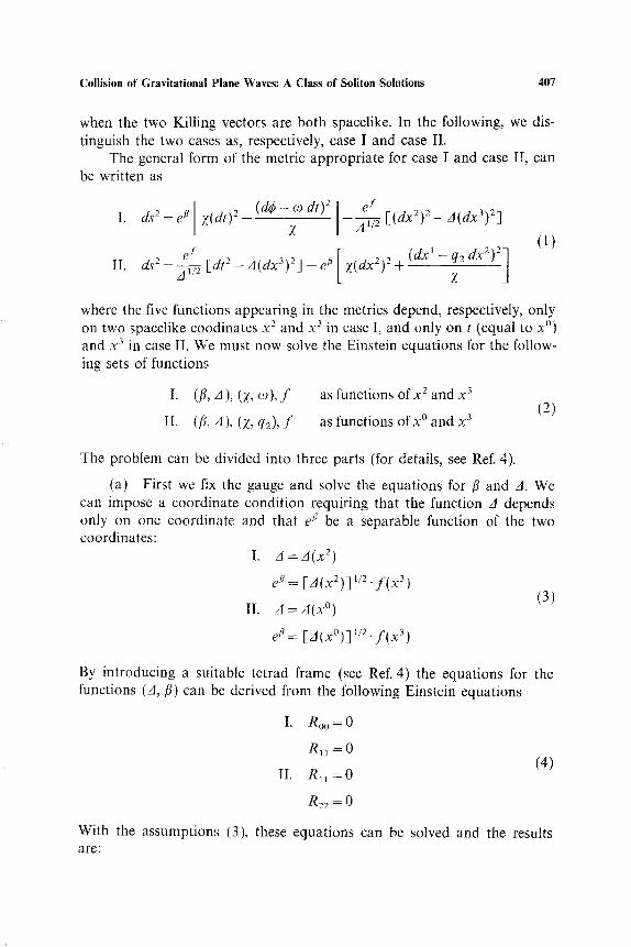
when the two Killing vectors are both spacelike. In the following, we dis- tinguish the two cases as, respectively, case I and case II.
The general form of the metric appropriate for case I and case II, can be written as
I. ds 2 e~[x(dl) 2 (dO-c~ er X ---~-T~ [(dx2)2+A(dx3) 2 ]
ef I II. dsZ=-A-~ [dt2- A(dx3) 2] - e ~ z(dx2)2+ (dx' - q z dx2)21 Z A
(1)
where the five functions appearing in the metrics depend, respectively, only on two spacelike coodinates x 2 and x 3 in case I, and only on t (equal to x ~ and x 3 in case II. We must now solve the Einstein equations for the follow- ing sets of functions
I. (/3, A),(X, co),f as functions of x2 and x 3 (2)
II. (/3, A), (Z, q2), f as functions of x ~ and x 3
The problem can be divided into three parts (for details, see Ref. 4).
(a) First we fix the gauge and solve the equations for /3 and A. We can impose a coordinate condition requiring that the function A depends only on one coordinate and that e ~ be a separable function of the two coordinates:
I. A = A(x 2)
e ~ ___ [A(x2)] ~/2 . f ( x 3)
rI. A = ~ ( x ~ (3)
eg= [A(x~ I/2-f(X 3)
By introducing a suitable tetrad flame (see Ref. 4) the equations for the functions (A, fl) can be derived from the following Einstein equations
I. R o o = 0
Nil =0
II. Rll =0 (4)
R22 = 0
With the assumptions (3), these equations can be solved and the results are:

408 Ferrari and Ibafiez
I. d = ( X 2 ) 2 - - 2 M x 2 + a 2
f = sin x 3 (5)
II. d = - - ( X 0 ) 2 "~ 2 T x ~ + a 2
f = sin x 3
where (/14, a) and (T, a) are integration constants. By introducing a new pair of coordinates ~/and #, given, respectively, by the relations
(X 2 -- M) I. r/= ( M 2 _ a2)1/2
= COS X 3
(x ~ T) (6) lI. r /= ( T 2 q'- a2)1/2
= COS X 3
one obtains for A and e ~ the following expressions
I. A = ( M 2 - a 2 ) ( t / 2 - 1 )
e ~ = (a6) 1/2
a = 1- - ,u 2
II. A = 1 - r /2
e#= (Z~a) 1/2
~ = 1 _ # 2
(7)
(In case II we measure the time x ~ in the unit (T2+ a2)1/2). Notice that in the first case q is a space l i ke coordinate and t/2 > 1, while in the second case t/is a t i m e l i k e coordinate, and /~2 < l.
The first part of the problem is then solved.
(b) The second part of the problem consists of finding and solving the equations for the functions (Z, co) and (Z, q;). They are given by
I. Ro o = 0
Rll = 0
Ro I = 0
II. Rll = 0 (8)
R22 = 0
R I 2 = 0

Collision of Gravitational Plane Waves: A Class of Soliton Solutions 409
It is possible to show that by introducing a function Z defined by
I. Z = ~ + i O
~ = (AcS)1/2/Z
1:/),2 = (~/Z 2) (D,3 (9)
0 3 = --(A/Z 2) 0),2
II. Z = Z + iq2
the equations (8) reduce to a single equation for the complex function Z which is the same equation in both cases
Re(Z){[(r /2- 1 ) Z , ] , n + [(1 -/~2)Z~],~} = ( t /2- 1 ) 2 2 + (1 -/~2)Z,2~ (10)
and this in the Ernst equation. If we are able to find solutions of this equation, the second part of the problem is solved.
(c) We must finally solve the equations for f They are, respectively
I. R23 = 0
G22 = 0
G33 = 0
II. R03 = 0
Goo = 0
G33 = 0
(11)
In these equations the function f is coupled to the function Z. Therefore, once a solution of equation (10) is known, it is only a technical problem to solve equation (11 ).
This brief review on the method shows that the heart of the problem is solving the Ernst equation since the gauge has already been fixed. Once the function Z has been found, one need only solve equations (11) for f and the complete solution is found.
However, another point must be stressed: stationary axisymmetric space-times and space-times with two spacelike Killing vectors satisfy the same Ernst equation. Therefore, if we know the solution for Z in one of the two classes, we can use the same funct ion Z to obtain the corresponding solution in the other class. In addition, let us note that in this method the procedure for obtaining new solutions from known solutions, but with dif- ferent Killing vectors, is not equivalent to a complexification of the coor-

410 Ferrari and Ibafiez
dinates, because the function Z is related to the metric functions in a dif- ferent way for the two classes of solutions.
Metrics with two spacelike Killing vectors can describe cosmological solutions and gravitational plane-wave solutions; the analogy just described suggests that cosmological and plane-wave solutions can be found as solutions corresponding to some stationary axisymmetric solutions and vice versa. Following this approach, it has been shown (Ref. 4) that the Schwarzschild and the Kerr metric are the solutions that correspond to the Khan-Penrose and to the Nutku-Halil metric, which describe, respectively, the collision of two impulsive, gravitational plane waves with collinear polarization (K-P) or with noncollinear polarization (N-H).
The second method for integrating the Einstein equations for the class of space-times we are interested in is the inverse scat ter ing method. In this section we describe it "by blocks" as we did for the first method, and in the next section we apply it to construct a class of exact soliton solutions. As in the first method, the search for solutions can be divided into three parts:
(a) choice of the gauge
(b) solution of the main equations which determine the metric
(c) construction of the remaining metric components
As in the previous analysis, we deal with stationary axisymmetric solutions (case I) and solutions with two spacelike Killing vectors (case II). We start with the following general form of the metric
I. as2 = _ f ( @ 2 + dz2 ) _ go~ dx o dx b (12)
II. ds2 = f ( dt 2 - dz2) - ga~ dx a dxb
where g~b is a two-dimensional matrix. In case I the metric functions depend on two spacelike coordinates (p and z equal to x 2 and x 3, respec- tively), while in the second case they depend on one timelike coordinate t (equal to x ~ and one spacelike coordinate z (equal to x3). Let us now analyze the content of each block.
(a) By making a coordinate transformation, it is always possible to make the determinant of g,b equal to
I. det(g) = _p2
II. det(g) = t 2 (13)
(b) The equations that lead to the Ernst equation, in the first

Collision of Gravitational Plane Waves: A Class o f Sol i ton Solutions 411
method, can be handled in a different way in order to write a single matrix equation for the matrix g = (gab)
I. (pg.pg l),p+(pg,zg-1),~=O (14)
II. (tg,,g-1),,-(tg,zg 1),z = 0
These equations can be solved by using the inverse scattering method, as has been shown by Belinski and Zakharov. The method consists in associating a linear eigenvalue problem with equations (14). From a known solution and the so-called "poles trajectories"
# k : ('Ok - - Z A7 [ - ( O k - - Z ) 2 - - 0~ 2 ] 1/2
where ~2= det(g), co~ are arbitrary complex or real constants, and k runs from zero to n, an arbitrary integer (the number of "solitons"), the integration of the equation can be done by algebraic manipulation. We do not enter into the details of this technique here since it has been extensively described in the references quoted in this paper.
(c) The third part of the solution consists in solving the equations for the function f, which are
I. ( l n f ) , p = - p ~ + ( @ ) - l t r ( U 2 _ V 2)
(ln f),= = (2p) -1 tr(U. V)
U = p g , p g-l, V = pg,= g-1 (15)
II. (ln f) , , = - t - l + (4t) -I tr(UZ + V 2)
( ln f ) ,== (2t) ~ tr(U. V)
U=tg,,g 1, V=tg,=g-1
Once the matrix gob has been determined, these equations can in principle be integrated and the complete solution found.
The block diagram of the two methods we have outlined suggests interesting analogies. In both methods we see that the central problem is to solve step (b), namely, the Ernst equation in the first method or the equations for gab by the inverse scattering technique in the second. The solutions of the Ernst equation have been extensively investigated, since its introduction by Ernst [10, 11 ] in 1968, and many classes of solutions are known. The technique for solving the equations (14) allows one to find new solutions depending on a known metric, which is assumed to be the "seed" metric, and the number of poles that certain properly defined functions must have. Let us note that in the inverse scattering method a new solution

412 Ferrari and Ibafiez
of Einstein's vacuum equation is generated from a known solution (the seed metric), both having the same Killing vectors. It has been shown [12] that there is a Backlund transformation which maps the old Ernst potential into the new one. However, in the method developed by Chandrasekhar and Ferrari, new solutions are obtained from known solutions, but (a) they have different Killing vectors and (b) they have the same Ernst potential.
It has been shown by Belinski and Zakharov that using the Minkowski metric as a seed metric, applying the method to the first group of equations (14), and imposing that there be two real poles and that the metric be diagonal, one obtains the Schwarzschild metric. Moreover, we show in the next section that by using as a seed metric the Kasner metric
ds2=t-2"t'2(dt2-dz2)-t2"~(dxl)2-t2S2(dx2)2 with s l + s 2 = l (16)
setting s 1 = s 2 = 1/2 and looking for the diagonal solution with two real poles, we obtain the Khan-Penrose solution. But we have said in the first part of this section that these two solutions are "analogous" in the sense that they are derived from the same Ernst potential. This fact suggests that the same analogy must exist between the two seed metrics when st = s 2 = 1/2. In fact, following the first method we have described, it is easy to show that both Minkowski and Kasner metrics, with st = s2 = 1/2, can be derived from the same Ernst potential
Z = I
But now a new question arises. We have seen that by using the Kasner metric with Sl = s2 = 1/2 as a seed for the inverse scattering method, we can obtain a "plane impulsive wave interaction" solution. Can the solution for arbitrary values of sl be a more general class of metrics describing the interaction of plane waves? The next section is devoted to answering this question.
3. A GENERAL S O L U T I O N FOR THE COLLISION OF GRAVITATIONAL PLANE WAVES
The class of solutions we derive in this section has been obtained via the inverse scattering technique, using as seed metric the homogeneous Kasner metric (16). The value of the parameters s t - -0 , Sa = 1 (or s t = 1, s2 = 0) correspond to flat space-time, while sl = s2 = 1/2 correspond to the axisymmetric Kasner metric.
Solutions obtained from the metric (16), with either one real pole or two complex poles, where given by Belinskii and Zakharov [2]. Sub-

Collision of Gravitational Plane Waves: A Class of Soliton Solutions 413
sequently, Carr and Verdaguer [13] examined the cosmological solutions generated by the metric (16) . The general expression, given in Ref. 13, for diagonal metrics with n po les /4 is (see equations (12), case II)
gll-----t n (klEI=l ~k) t2Sl
g22 = t2/gll (17)
2SlS;tn(n--2+4s2)/2 .k~3 2s2 rI-Ik,l~l,k>l(.k__.l ) f= t L HE 2- J 1
We study solution (17) for two real poles (n--2) and assuming
*'1 = o )1 - z - [ ( o ) 1 - z ) 2 - t 2 ] 1/2
( 1 8 ) ].12=032--Z-}" [(O)2--Z)2--12] I/2, (.0 1 = --(.02= 1
(Notice that this derivation of the poles is completely similar to that used to obtain the Schwarzschild metric from the Minkowski metric in cylin- drical coordinates [13]. In that case o)= ~ = -o)2, and co is the mass of the central body). Let us now consider the following change of coordinates
t = sin ~b sin 0, z = cos ~b cos 0, 0 ~<~b ~rc, 0 ~ < 0 4 ~ (19)
The expressions (18) make the solution defined in the region outside of the two light-cones
( 1 - - z ) 2 - - t 2 = 0 and ( - 1 - z ) 2 - t 2 = 0
The change of coordinates (19) restricts the solution to the region between the two ligh-cones.
The final expression of the metric is
ds 2 = (sin ~b sin 0)-2s:2(1 + c o s ~ ) 2 s 2 ( 1 - COS ~)2Sl(d~2 - dO 2)
1 + cos ~b (dx2)2 1 - c o s ~b (dx~)2 - (sin ~b sin O) 2~ 1 - c o s r - (sin ~b sin 0) 2sl 1 + cos~
S 1 -}-S 2 ~-- 1 (20)
When s 1 = s 2 = l / 2 the metric (20) becomes the Khan-Penrose solution in the region of interaction between the two impulsive gravitational waves. Therefore, we expect that the uniparametric family of solutions (20) will represent a generalization of this solution.
In order to prove this statement, several steps must be followed:
1. We choose a null N - P tetrad and compute the Weyl scalars.
2. We introduce null coordinates u and v and discuss the singularities of the Weyl scalars.

414 Ferrari and Ibafiez
3. We extend the metric prior to the instant of collision, across the null surfaces u = 0 and v = 0, and see if the extension is always possible.
4. We check that all the junction conditions across the null boundaries that separate the different regions of the resulting space-time are verified.
Points (3) and (4) will be discussed in the next section. The metric (20) has the following form
where
ds 2 = f(d~b 2 - dO 2) - g l l ( d X l ) 2 - g 2 2 ( d x 2 ) 2 (21)
f = (sin ~b sin 0)-2"x'2(1 + c o s ~)2s2(1 - C O S ~) 2sl
gll = (sin ff sin 0)2~(1 - c o s ~b)/(1 +cos ~b)
g22 = (sin ~b sin 0)2"2(1 + cos q~)/(1 - c o s ~b)
(22)
By introducing the null tetrad
1
1 i '= ~ (8 ~ - 8 o ) (23)
1 ( 1 , )
(with rh-rh* = -1 , d. [= 1), it is easy to verify that the nonvanishing Weyl scalars are (see, e.g., Ref. 7)
~o = - L [ - 281 s2(s2 - S l ) cos(~b + 0) sin(~b - 0) ZJL sin ~b sin 0 F 6sis 2 sin2 ~ sin 0
SlS2(Sl-S2) (3 -S lS2) ( s1-s2) 3(sl-s2)2cos~b] + sin 2 0 sin 2 ~b sin--~ J
~4 = -- _j ,_2slsz(S2 -- Sl) sin ~ sin 0 6SlS2sin2cbsinO ~ sin20
(3--8182)($1--82) 3(81- 82)2 COS ~7 - sin 2 ~ , s-i~n2 ~b j
1 F sis2 1--81s2 (S1--S2) COS ~ ~ U 2 = 2 " f L ~ - I sin2----~ § sin 2 ~b
(24)

Collision of Gravitational Plane Waves: A Class of Soliton Solutions 415
Let us now introduce a couple of null coordinates
u = cos(~b + 0)/2, v = sin(0 - ~b)/2 (25)
In terms of these coordinates the metric (20) takes the form
ds 2 = jT(u, v) du d v - g11(u, v)(dxl) 2 - g22(u, v)(dx2) 2 (26)
where 7 is connected to the function f (see equation 22) by the relation
f _ 8f (27) sin ~ + sin 0
Moreover the tetrad (23) expressed in these coordinates is
/'~= --(21/2/_71/2)( l -- t~ 2) -1/4( 1 -- U 2) 1/4 ~u
]'= _(21/2/~I/2)(1 _ v2)1/4(1 _ u 2) -1/4 0c (28)
rfi = (1/2'/2)[ (1/g,, '/2) Ox, + (i/g22 '/2) ~x2]
The metric (26) is defined inside the circle (see Fig. 1)
u 2 + v 2= 1
~, ~=1 ~ 0
Z region u ~=,ff:O v : l , v - ~ : 0
<D-- ~tu =-1 u=O} ~=~ ~ : ~ / v = ( ~ v=-I -~=0
Fig. 1. Four regions of space-time.

416 Ferrari and Ibafiez
But, if we now require it to represent the collision of two gravitational waves, we must restrict its domain of validity to the region
0~<u~<l and 0~<v~<l
v~>0 u~<0
(we call it region IV; see Sect. 4) and, thus, we extend the metric to the two regions
0~<u~<l and 0~<v~<l
v ~ 0 u~<0
requiring that in each of these two regions there is a single plane wave. We now analyze the behavior of the Weyl scalars in region IV, looking for the values of s~ and s2 for which they are singular in this region, disregarding the possible singularities which appear in the other three quadrants of Fig. 1, because they will be eliminated by the extension.
Let us now write the Weyl scalars (24) in the following form
(sin 0 sin r kl + + To, T4 ~ (1 + cos r - c o s r 1 - c o s 2 r
ks cos 0 + k 6 cos 0 cos q~q k4 cos ~b -~ J (29) + 1 - cos 2 ~b sin 0 sin ~b
(sinOsinO)2s~s~ I k'~ k~+k'3c__osO] ~t2---~(l+cosq~)2S2(l_cos~)2s I ~ - t - l_cos2q~ j
where
kl = --2sl s2(sl -- s2)
k2 = sls2(sl - s2)
k 3=- - ( 3 - s i s 2 ) ( s 1 -$2 )
k 4 = - ( 3 - 6s1s2)
k s = ++_6sis2 (+ for gt o, - for gt4)
k6= -}-2s1s2(s I --$2) (n t- for 5u0, - for 5u4)
k'~ = -s~s2
k~= - ( 1 - s ~ s 2 )
k3= --(s~-s2)
(3o)

Collision of Gravitational Plane Waves: A Class of Soliton Solutions 417
O n t h e n u l l b o u n d a r i e s ( s e e F i g . 1)
0 ~ u < l v = 0 , 0 ~ v < l u = 0
7"[" 7~ o < ~ f o < ~ < ~
0 < 0 ~ ~ < 0 < ~
the Weyl scalars are regular. The arc AD has the equat ion
u 2 + v 2 = 1 and
O~<O~<rc, ~b=0
Let us exclude, for the momen t , the points A and D, the only points where sin 0 = 0. The singularities can arise f rom the terms that are zero when ~b = 0; therefore, we write the Weyl scalars in the following form
ka ~'o, ~4-, (1 + cos ~)s~(~-'~)(1 -cos ~)s,(~-,~)
kb + (1 + cos ~ ) s ~ - , ~ ) + ~(1 - cos ~ ) s ~ ,~)+~
k~ +
(1 § cos ~)~2(2-s~)+ 1/2(1 _ cos @)st(2-,z)+ a/2
k , = [k l + (kz/sin z 0) ] (s in O) 2s~s2
kb = (k3 + k4 cos ~b)(sin 0) 2~s2 (31)
k~ = (k 5 cos 0 + k 6 cos 0 cos ~b)(sin 0) 2~1'2
~.t 2 ----)
k , a
k;=
k" (1 + cos ~ )~(2-s ' ) (1 - c o s ~) ,~2 ,~)
k; +
(1 + COS q~)s;(2- sl)+ 1(1 _ COS ~)sl(2-s2)+ 1
(k'l/sin 20)(sin O) 2sIs2
(k; + k; cos ~b)(sin O) 2s~'~
F r o m equat ions (31) it is clear that ~2 will be regular for ~b=0 if the following two condi t ions are s imul taneously verified
$ 1 ( 2 - - $ 2 ) < 0 (32)
s ~ ( 2 - s z ) + 1 < 0

418 Ferrari and Ibafiez
Remembering that s2~- -1 -s l , it is easy to verify that equations (32) are not compatible; therefore, 7t2 is always singular on AD, except when k'a = k~ = 0, and this happens only when
S1=0 (33)
$2:1
Moreover, ~o and 7~4 will be regular on AD if the following three con- ditions are simultaneously verified
S l ( 2 - s 2 ) < 0
S1(2- S2)+ 1 < 0 (34)
s1(2 - s2) + �89 < 0
As before, they are not compatible, and therefore ~0 and ~u 4 are always singular on AD, except when k~ = kb = kc = 0, and this is true only when condition (33) is satisfied.
In conclusion, the Weyl scalars are always singular on the arc A D ( u 2 + v2= 1, 0 ~< u < 1, 0 ~< v < 1), except in one degenerate case (eq. 33), which will be discussed in Section V.
A similar analysis for points A and D shows that the behavior of the Weyl scalars is the same as we have now discussed.
4. EXTENSION OF THE METRIC AND I N T E R P R E T A T I O N OF THE S O L U T I O N
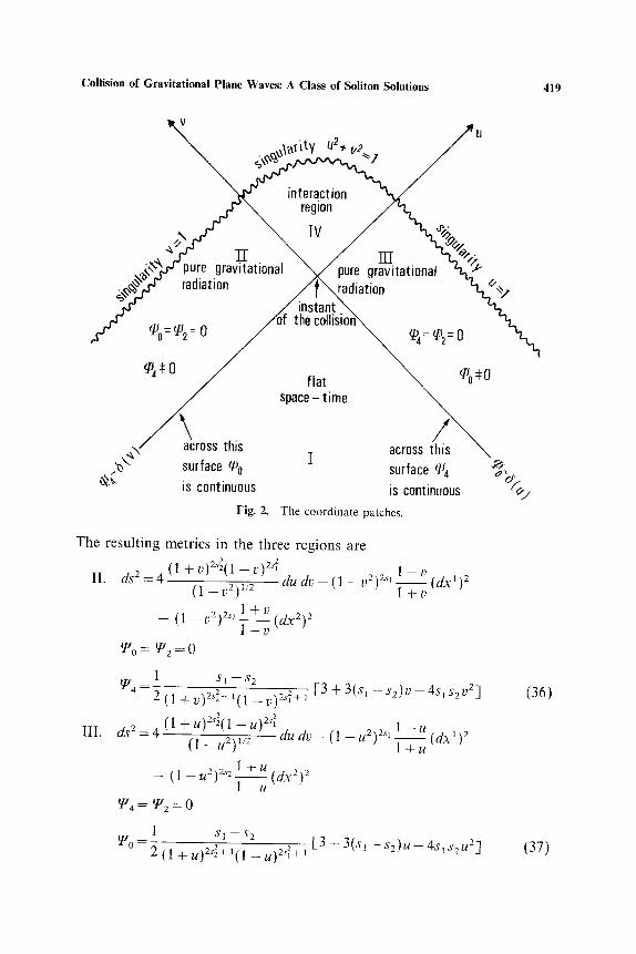
Let us first divide the space-time into four regions (see Fig. 2)
region I u < 0 v < 0
region I! u < 0 v > 0
regionIII u > 0 v < 0
region IV 0 ~ < u < l 0 ~ < v < l
As we have shown in Section 3, the class of solutions given by the metric (20) is defined in re~ion IV. Following Khan and Penrose, we extend the metric in regions I, II, and III, changing the coordinates u and v by
u ~ u H ( u ) and v ~ vH(v ) (35)
Collision of Gravitational Plane Waves: A Class of Soliton Solutions 419
~V a~itu u2,
,,_tx.tvx~ _ k 2"~ 7
"- E pure gravitational radiation
%:e2:o
~ o
\.~,/ across this ~ surf,3ce ~o
is continuous Fig. 2.
interactiol ~ ~ ) # , region ,Qv
, ~ pure gravitational ' . 2 ,at,o ff the collision'x. " h . ,
flat ~ q~o*O space - time " ~
I across this \ surface ~4 "~o' is continuous @~./
The coordinate patches.
The resulting metrics in the three regions are
II. d s 2 = 4 ( l + v ) 2 " ~ ( 1 - v ) 2 s ~ 2 2si l - u ( l _ v 2 ) , / 2 d u d v - ( 1 - v ) ~-~v(dx~)2
III.
- (1 _ ~)~-~ 11_~_+ vv (d~)~
~o = T2 = 0
! s~ - s 2 ~['r ~----~ (1 "{- /))2s~ + 1(1 -- u)2s2+ 1 [3 + 3(s~ - s 2 ) v - 4Sl s2 v 2 ]
ds 2 = 4 (1 + u)2S~(1 - u)2S~ (1 _ u2)ln d u d v - ( 1 - u 2 ) 2"~ 1 - u )2 7-T-~ (dx'
l + u - (1-u2)2s2~_u(dX2)2
~J4 ~-" ~7J2 = 0
~ 0 = ~ - - S1 --$2 ( l+u)2S~+J(1-u)2S~ + [3+3(s 1 - s 2 ) u - 4 s l s 2 u 2]
(36)
(37)

420 Ferrari and Ibafiez
IV . ds2=4 du d v - (dx1)2- (dx2) 2
g*4 = gt0 = g*2 = 0 (38)
We, therefore, obtain flat space-time in region I, and a metric of type N in regions II and III, where the only nonvanishing Weyl scalars are either g*4 or 7*o. In these two regions the solution represents a plane gravitational wave moving to the right (region II) or to the left (region III). They collide when u = v = 0 and their focussing on the surface u2+ v 2= 1 in region IV produces the singularity of the Weyl scalars on this surface, as discussed in Section 3.
But in order to be sure that this interpretation is correct, we must check that all the junction conditions across the surfaces which separate the different regions are satisfied. Because the metric is symmetrical in u and v, it suffices to check that these conditions are satisfied across the two regions
a . I V --+ II (u = 0)
b. III --+ I (u = 0)
Case (a) ( j ~ I V ) u = 0 =f", (gP~), = o = g]~, (gz2)~=0-IV - g~2(39)
the metric is continuous.
( f~v~ 2(s2_s,)_v(s2_s,)2 (sTir) ylVJu=O- i - v 2 = ~'H u=O
glV \ II 61,,~| _ 2 +4s~1)=f g,a,v~ IV i)2
\ g l l )u=O 1 - \-7~1),=o IV II (g22,~'] _2-4si1)_(g22,~)
-U/-+-" - - -2f i - - \ g22 , ]u -O 7 ~ - - 7 - - - \ g22 ,]u=O
( 1 - 1 ) : ) lj: u : o = ~
IV lI ( g , l , u ) - - - - 2 (gll,u~
-- - - V2)1/2 ~--- 0 \ ) . :o (1 L :o gIV \ / gII \ c5 22,u ~ - - 2 f~22'u/ = 0
iv \ g22//~ = o g22 )u=O (1 --/)2) lj2 II
(40)
The first derivatives of the metric with respect to v are continuous; the ones with respect to u are not. The same is true for the second derivatives and the jump presented by those with respect to u is
(41)

Collision of Gravitational Plane Waves: A Class of Soliton Solutions 421
7<iv ?iv = ~ H(u)+~6(u)
IV IV g.b,.. gab~ uu H(u) + ~ 6(u) gab gIV g,b
(42)
The Weyl scalars have the following behavior
~ 4 = (~r u=O - - __ ~ I I u=O ~'r i s c o n t i n u o u s
1 1 6(u) ~o = 7tY H(u) q 2 (1 + v)2s2(1 - u) 2s~ (1 - - 122) 1/2
~F-/2 = ~P~v H(u)
(43)
According to the O'Brian and Synge [14] conditions, we can allow a dis- continuity in certain first derivatives of the metric functions across the null boundary u = 0 , if they do not produce any source term in Einstein's equations.
In our case, all functions and their first and second derivatives with respect to v are continuous on u = 0; therefore, we need only to check that the components of the Ricci tensor in which second derivatives with respect to u appear are zero on u = 0. This component is
l (gl,Vu g,V , jr_ 22,u} ~)(bl) = 0 Roo = RgH(u) +~ -=iv-
\ g l l g22 J (44)
IV__ But Roo i 0 , since the Einstein equations are satisfied in region IV; moreover, from equations (41), it is clear that the coefficient of the function is zero. Therefore, the Einstein equations are satisfied on the null boundary u = 0.
Case (b) A similar situation arises when we analyze the behavior of the metric functions and their first and second derivatives on the surface u = 0, which separate region I l I from region I. The metric is again con- tinuous. Moreover
\ ] 'D ' ) , ,=o = ~ - - = o k 7 ' ) . : o kg~ ; ' ) . =o \ 7 ~ - . I . = = o
(_.i . (g',2v) g22.~ _ = 0 (45) - z m - . - ) . : o g22 / u = O
84219'4 7
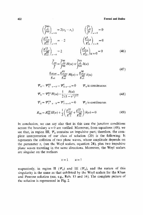
422 Ferrari and Ibafiez
/ jTf ) = 2(s2- s~) (7 A
~ 0
( ~ I I I \ g l l , u ] = - - 2 (g]l,u']
)o =o 1 :o = ~ / g l I I \
/ ,22.,~ = 2 \-~22 ,]u = 0 = 0 (46)
J~,, u u
?
gab,uu
? f f I ~ l I I
- - ? I I I H(u) + ~ 6(u)
~III ~III _g~b,~ H(u) + ,gab,u (~(H)
- - ~III gab gab gab
(47)
~F'/4 = ~IY-/~ II = 0 gt 4 is continuous
1 6(u) 7s~ = ~I~ + 2 (1 - v 2 ) 1/2 (48)
~T/2 = ~r : 0 ~ : 0 = ~ff~ ~ = 0 ~u 2 is continuous
/ _III ~III \ Roo = Rlo~ H(u) + ~ I g ~l'--~" + g22,u] 6(u)= 0 \ gpi -:irc,
N22 / (49)
In conclusion, we can say also that in this case the junction conditions across the boundary u = 0 are verified. Moreover, from equations (48), we see that, in region III, ~o contains an impulsive part; therefore, the com- plete interpretation of our class of solution (20) is the following: It represents the collision of two plane waves, whose amplitude depends on the parameter sl (see the Weyl scalars, equation 24), plus two impulsive plane waves traveling in the same directions. Moreover, the Weyl scalars are singular on the surfaces
v = l u = l
respectively, in region II (gt4) and III (gto), and the nature of this singularity is the same as that exhibited by the Weyl scalars for the Khan and Penrose solution (see, e.g., Refs. 15 and 16). The complete picture of the solution is represented in Fig. 2.

Collision of Gravitational Plane Waves: A Class of Soliton Solutions 423
5. S O M E D E G E N E R A T E CASES
There are two part icular cases of the general interesting to investigate
1. s I = 0 , s 2 = l
2. sl = 1, s 2 = 0
The metric (20) becomes
solution
1 -cos@ (dxl)2 1. ds2=-( l q-cos@)2(d(j~2-dO 2 ) 1 q- COS @
- sin 2 0(1 + cos @)2(dx2)2
1 -}- COS @ ( d x 2 ) 2 2. d s 2 = ( l - c o s @ ) 2 ( d @ 2 - d 0 2 ) 1 - c o s @
- sin 2 0(1 - c o s @)2(dxi)2
and the Weyl scalars are
which are
(50)
3 1 1. ~0 = ~ 4 = ~ 2 -
2(1 + cos @)3 2(1 + cos @)3 (51)
3 1 2. ~ 0 = ~r/4 - ~ f f2 -
2(1 - c o s @)3 2(1 - c o s @)3
Both metrics are type D and, by a suitable ro ta t ion of the tetrad (23), the Weyl scalars become
1 1. ~Jo = ~ 4 = 0 I//2 =
(1 + cos r (52)
1 2. ~ 0 = ~/4 = 0 ~ 2 =
(1 - - COS @)3
It is easy to verify that the two metrics (50) are the Schwarzschild metric inside the horizon. In fact, if we write the Schwarzschild line element in the usual Boyer -Lindquis t coordinates, putt ing M = 1, we get
ds 2 = E1 - (2/r)] dt 2 - - E1 - (2/r)] -1 dr 2 _ r2(dO 2 + sin 02 d i p 2 ) (53)
and if we put
cos @ = r -- 1 o r
cos @ = 1 - r

424 Ferrari and Ibafiez
we immedia te ly obtain, respectively, cases 1 and 2 of the metr ic (50), and the nonvanish ing Weyl scalar assumes the form
~2 = --1/r3
The two metrics have the following differences: the metr ic 1 is not singular in region I V on A D (see Fig. 1), where cos ~b = 1. This surface cor responds to the black hole hor izon r = 2. The singularity r = 0 cor responds to the arc BC and the point u = v = 0 cor responds to r = 1. The extension discussed in the previous section is always possible (all the junct ion condit ions are satisfied) and the Weyl scalars in regions II, I I I , and I are
I. ~Uo = gt4 = ~2 = 0
3 Ii. ~ 4 -
2(1 +/))3
3 III . g~o - 2(1 + U) 3 ~g'r ~ ~ 2 = 0
~0 = g~2 = 0 (54)
They are not singular on u = 1 and v = 1 in regions I I and III . Neverthless, there is a curva ture singularity on these surfaces, as it can be seen by calculating the extrinsic curvature in these two regions (see, e.g., Ref. 16).
On the contrary , the metric 2 is singular in region IV on A D and, in this case, cos ~b= 1 cor responds to the Schwarzschild singularity r = 0 . Region IV represents, in this case, the Schwarzschild region for r which ranges f rom 0 to 1. When we extend the metric we obta in
I.
I I .
~ o = ~ 4 = ~2 = 0
3 ~lf'g4 = ~t[/4 = "] 2(1 _/))3 ~'tO = ~ 2 = 0 ( 5 5 )
3 III . g to= q 2 ( l _ u ) 3 ~4 = ~ 2 = 0
and the singularity on u = 1 and v = 1 occurs, as in the other cases previously discussed. In this case we can say that there are two par t icular plane waves whose collision produces a region of space- t ime where the gravi ta t ional field is the Schwarzschild field for 0 < r < 1 (M = 1) and a singularity in r = 0, but this singularity is not hidden by a horizon.

Collision of Gravitational Plane Waves: A Class of Soliton Solutions 425
6. CONCLUDING REMARKS
In this paper a new class of solutions of the vacuum Einstein equations has been obtained. It describes the head-on collision of two linearly polarized impulsive gravitational plane waves of the same polarization, each supporting a gravitational plane wave. The solution has been obtained by using soliton techniques, and it has been extended and inter- preted following the approach described in Ref. 4.
A comparative analysis of two possible methods of finding solutions with two Killing vectors of Einstein's equations has been given. Once a gauge has been fixed, the solution of the Ernst equation or the solution of the matrix equations via the soliton techniques, in principle, allows the complete determination of the metric.
Moreover, the analogies described in Ref. 4 between solutions with two spacelike Killing vectors and stationary-axisymmetric solutions suggest that once a solution of one class has been determined using one of the two methods, the corresponding solution of the other class can be calculated by using the same Ernst potential.
Many problems can be analyzed following this approach. A sub- sequent paper will investigate whether the class of solutions presented in this paper has a corresponding class of physically meaningful solutions in the stationary-axisymmetric case. Moreover, the class of nondiagonaI solutions that are obtained by using the soliton techniques and using the Kasner metric as a seed will be calculated, and the possibility that this class of solutions can be interpreted as the general solution describing the collision of noncollinear gravitational plane waves will be considered.
REFERENCES
1. Belinskii, V. A., and Zakharov, V. E. (1979). Soy. Phys. JETP, 50(1), 1. 2. Belinskii, V. A., and Zakharov, V. E. (1978). Soy. Phys. JETP, 48(6), 985. 3. Chandrasekhar, S. (1978). Proc. R. Soc. Lond., A358, 405. 4. Chandrasekhar, S., and Ferrari, V. (1984). Proc. R. Soc. Lond., A396, 55. 5. Khan, K. A., and Penrose, R. (1971). Nature, 229, 185. 6. Nutku, Y., and Halil, M. (1977). Phys. Rev. Lett., 39, 1379. 7. Ibafiez, J., and Ferrari, V. (1987). Gen. Relativ. Gray., 19, 383, 8. Chandrasekhar, S., and Xanthopoulos, B. C. (1985). Proc. R. Soc. Lond., A402, 37. 9. Chandrasekhar, S., and Xanthopoulos, B. C. (1985). Proc. R. Soc. Lond., A398, 398.
10. Ernst, F. J. (1968). Phys. Rev., 167, 1175. l l . Ernst, F. J. (1968). Phys. Rev., 168, 1415. 12. Cosgrove, C. M. (1982). J. Math. Phys., 23(4), 615. 13. Carr, B. J., and Verdaguer, E. (1983). Phys. Rev., D28(12), 2995. 14. O'Brian, S., and Synge, J. L. (1952). Commun. DubL Inst. Adv. Stud., A9. 15. Bell, P., and Szekeres, P. (1974). Gen. Relativ. Gray., 5, 275. 16. Matzner, R. A., and Tipler, F. J. (1984). Phys. Rev., D29, 1575.