Embed Size (px)
Citation preview

THÈSE NO 3378 (2005)
ÉCOLE POLYTECHNIQUE FÉDÉRALE DE LAUSANNE
PRÉSENTÉE À LA FACULTÉ SCIENCES DE BASE
Institut de mathématiques
SECTION DE MATHÉMATIQUES
POUR L'OBTENTION DU GRADE DE DOCTEUR ÈS SCIENCES
PAR
ingénieur civil de l'Ecole des Mines de Nancy, Franceet de nationalité française
acceptée sur proposition du jury:
Lausanne, EPFL2005
Prof. Th. Liebling, directeur de thèseDr J.-A. Ferrez, rapporteurProf. S. Luding, rapporteur
Prof. A. Quarteroni, rapporteurProf. J. Rambau, rapporteur
ON THE BEHAVIOR OF SPHERICAL AND NON-SPHERICAL GRAIN ASSEMBLIES,
ITS MODELING AND NUMERICAL SIMULATION
Lionel POURNIN

iii
Acknowledgements
Since acknowledgments is an English word, I feel terribly encouraged to begin them asany reasonable frenchman would, en Anglais. Yet, this is not because I am reason-able, nor is it for the sake of tradition that I first think here to my supervisor, ThomasLiebling. He instigated this work, and without his guidance I would not have beenable to write much of it. More than this, his kindness and humanity have been pre-cious to me over the last few years. I wish to thank my referees, Jean-Albert Ferrez,Stefan Luding, Thomas Mountford, Alfio Quarteroni and Jörg Rambau for their care-ful reading of my thesis and their helpful comments. And since I am reasonable andFrench, I will go on writing in a more familiar way.
Je voudrais remercier ma famillle, mes sœurs, mes parents et ma grand-mère pour bienplus que ce que je ne pourrais formuler ici. Je pense aussi a Nicole, Denis, Emmanuelleet Véronique Gira. Merci pour votre soutien et votre amitié au travers de toutes cesannées, dans les épreuves comme dans les moments de joie.
Cette page j’aurai pu l’écrire d’un petit coin vert de Roumanie, de Satu-Mare ou dupays de Oas. Beaucoup des idées qui ont conduit à cette thèse ont été formulées là-bas,à Negresti-Oas et à Gherta Mica. Imi e dor de acolo, si de tine, Lum. Multumesc pentrutot.
Une autre de mes pensées ici est pour Frédéric qui dans sa Syrie adoptive, au monastèrede Mar-Musa, se charge de la prière que trop souvent, la paresse me fait remplacer parun sommeil profond mais tout de même bien agréable.
Je pense aussi a ceux avec qui j’ai vecu durant les années qu’ont duré ma thèse, dontplusieurs générations de membres du ROSO. Je remercie particulièrement Marc-OlivierBoldi pour son amitié, Marco Ramaioli et Michel Tsukahara pour leur compagnie detous les jours, mais aussi des statisticiens, géomètres, algébristes, peintres en bati-ment, bergers du Jura, banquiers genevois, petits patrons et chanteurs populaires :Christophe Osinski, Hugo Parlier, Gérard Maze, Sandrine Péché, Sylvain Sardy, An-drei Zenide, Jerôme Reboulleau et Roland Rozsnyo. Comment oublier ici le séminairehomonyme, réservé aux grandes personnes, et duquel on aurait pu dire (bien trop tardprobablement) qu’il fût le ferment des grandes avancées de ce siècle ?
Je tiens a remercier quelques Mineurs de Nancy : Alain Mocellin à qui je dois ce par-cours, mais aussi Guy Raguin, Matthieu Delost, Fabrice Morin et Géraldine Plas pources années pleines de rebondissements. Je pense aussi à toi, Romain, où que tu sois.
Last but not least, I would like to send some greetings to the members of a Frenchdemomaking-packing group, who made nice things on a famous 16-32bit computer be-tween 1989 and 1993: Thierry Lemoult, Matthias Baillet, Christian Sabarot and KarimZiouani.
This project was partially funded by the Swiss National Science Foundation, grant# 200020-100499/1.


v
Abstract
This thesis deals with the numerical modeling and simulation of granular media withlarge populations of non-spherical particles. Granular media are highly pervasive innature and play an important role in technology. They are present in fields as diverseas civil engineering, food processing, and the pharmaceutical industry. For the physi-cist, they raise many challenging questions. They can behave like solids, as well asliquids or even gases and at times as none of these. Indeed, phenomena like granularsegregation, arching effects or pattern formation are specific to granular media, henceoften they are considered as a fourth state of matter.
Around the turn of the century, the increasing availability of large computers made itpossible to start investigating granular matter by using numerical modeling and simu-lation. Most numerical models were originally designed to handle spherical particles.However, making it possible to process non-spherical particles has turned out to beof utmost importance. Indeed, it is such grains that one finds in nature and manyimportant phenomena cannot be reproduced just using spherical grains. This is themotivation for the research of the present thesis.
Subjects in several fields are involved. The geometrical modeling of the particles andthe simulation methods require discrete geometry results. A wide range of particleshapes is proposed. Those shapes, spheropolyhedra, are Minkowski sums of polyhe-dra and spheres and can be seen as smoothed polyhedra. Next, a contact detectionalgorithm is proposed that uses triangulations. This algorithm is a generalization of amethod already available for spheres. It turns out that this algorithm relies on a pos-itive answer to an open problem of computational geometry, the connectivity of theflip-graph of all triangulations. In this thesis it has been shown that the flip-graph ofregular triangulations that share a same vertex set is connected.
The modeling of contacts requires physics. Again the contact model we propose isbased on the existing molecular dynamics model for contacts between spheres. Thosemodels turn out to be easily generalizable to smoothed polyhedra, which further mo-tivates this choice of particle shape.
The implementation of those methods requires computer science. An implementationof this simulation methods for granular media composed of non-spherical particleswas carried out based on the existing C++ code by J.-A. Ferrez that originally handledspherical particles.
The resulting simulation code was used to gain insight into the behavior of granularmatter. Three experiments are presented that have been numerically carried out withour models. The first of these experiments deals with the flowability (i. e. the abil-ity to flow) of powders. The flowability of bidisperse bead assemblies was found todepend only on their mass-average diameters. Next, an experiment of vibrating rodsinside a cylindrical container shows that under appropriate conditions they will or-der vertically. Finally, experiments investigating the shape segregation of sheres andspherotetrahedra are perfomed. Unexpectedly they are found to mix.

vi RÉSUMÉ
Résumé
Le sujet de cette thèse est la modélisation et la simulation numérique de milieux gran-ulaires composés de grains non sphériques. Les matériaux granulaires abondent dansla nature et ont une place importante dans la technologie. On les trouve dans des do-maines aussi divers que le génie civil, l’industrie agro-alimentaire ou l’industrie phar-maceutique. Pour le physicien, ils sont d’autre part la source de nombreuses questions.
A la fin du siècle dernier, l’augmentation de la puissance de calcul des ordinateurs arendu possible l’utilisation de la simulation numérique pour l’étude les milieux gran-ulaires. Au départ, la plupart des modèles numériques etaient développés pour traiterdes particules sphériques. Pouvoir simuler des grains non-sphériques s’est révélé étred’une importance cruciale. En effet, les particules que l’on trouve dans la nature sontnon-sphériques et un grand nombre de phénomènes importants ne peuvent pas êtresreproduits avec des grains spheriques. Ceci constitue la motivation de la rechercheprésentée dans cette thèse.
Il s’agit d’un travail pluridisciplinaire. La modélisation géométrique des particules etles méthodes de simulation se basent sur des résultats de géométrie algorithmique.Une grande variété de formes de particules est proposée. Ces formes ou spheropolyè-dres, sont des sommes de Minkowski de polyèdres et de spheres et peuvent être vuescomme des polyèdres lissés. Ensuite, un algorithme de détection des contacts utilisantdes triangulations est proposée. Cet algorithme est la généralisation d’une méthodedéjà implémentée pour les sphères. Il se trouve que la convergence de cet algorithmedépend de la réponse à un problème ouvert en géométrie algorithmique, la connex-ité du graphe des flips de toutes les triangulations. Dans cette thèse, la connexité dugraphe des flips des triangulations régulières qui ont en commun leur ensemble desommets a été démontrée.
La modélisation des contacts s’appuie sur la physique. Le modèle que nous pro-posons est basé sur les modèles de type dynamique moléculaire pour les contacts entresphères. Ces modèles se généralisent facilement à nos polyèdres lissés, ce qui constitueune motivation de plus pour choisir cette famille de formes.
L’implémentation de ces méthodes pour des milieux granulaires composés de partic-ules non-sphériques a été faite à partir du programme écrit en C++ par J.-A. Ferrezpour la simulation numérique de grains sphériques.
Ce programme a ensuite été utilisé pour étudier certains phénomènes liés aux milieuxgranulaires. Trois expériences ont été conduites numériquement avec nos modèles.Avec la première de ces expériences, la coulabilité des poudres, c’est-à-dire la facilitéavec laquelle elles peuvent couler, a été étudiée. Il s’est trouvé que la coulabilité des en-sembles de sphères bidisperses ne dépend que de leur diamètre moyen en masse. En-suite, une expérience consistant a faire vibrer des particules alongées dans un containercylindrique montre que sous certaines conditions ces particules vont s’ordonner verti-calement. Enfin, des expériences de ségrégation par formes de sphères et de sphéroté-traèdres montrent que ces deux formes vont avoir tendance à se mélanger.

Contents
Introduction 1
Inter-particulate contact modeling . . . . . . . . . . . . . . . . . . . . . . . . . 2
Collision detection . . . . . . . . . . . . . . . . . . . . . . . . . . . . . . . . . . 2
Is the flip-graph of regular triangulation connected ? . . . . . . . . . . . . . . . 3
Granular matter and numerical simulation . . . . . . . . . . . . . . . . . . . . 3
I Methods 5
1 Mathematical preliminaries 7
1.1 Polyhedra and complexes . . . . . . . . . . . . . . . . . . . . . . . . . . . 7
1.2 On the flip-graph of regular triangulations . . . . . . . . . . . . . . . . . 10
1.2.1 Geometric bistellar operations . . . . . . . . . . . . . . . . . . . . 11
1.2.2 Monotone connectivity of the graph of regular triangulations . . 12
1.3 Weighted Delaunay triangulations and power diagrams . . . . . . . . . . 14
2 The Distinct Element Method 19
2.1 A model for particle shapes . . . . . . . . . . . . . . . . . . . . . . . . . . 20
2.1.1 Contacts and overlaps between particles . . . . . . . . . . . . . . 21
2.2 Contact force modeling . . . . . . . . . . . . . . . . . . . . . . . . . . . . . 25
2.3 Tuning molecular dynamics models with real experiments . . . . . . . . 27

viii CONTENTS
3 A triangulation-based contact detection method 31
3.1 Spherical particles . . . . . . . . . . . . . . . . . . . . . . . . . . . . . . . . 31
3.2 Non-spherical particles . . . . . . . . . . . . . . . . . . . . . . . . . . . . . 32
3.2.1 Covering the particles with spheres . . . . . . . . . . . . . . . . . 33
3.3 Building and handling the triangulation . . . . . . . . . . . . . . . . . . . 38
3.3.1 Building the initial triangulation . . . . . . . . . . . . . . . . . . . 38
3.3.2 Triangulation Maintenance . . . . . . . . . . . . . . . . . . . . . . 39
4 Some implementation details 41
4.1 Intoduction . . . . . . . . . . . . . . . . . . . . . . . . . . . . . . . . . . . . 41
4.2 Structure of the simulation environment . . . . . . . . . . . . . . . . . . . 42
4.3 Enhancing the robustness of triangulation maintenance . . . . . . . . . . 44
4.4 Experimental complexity analysis . . . . . . . . . . . . . . . . . . . . . . 46
4.5 Some inertia matrices . . . . . . . . . . . . . . . . . . . . . . . . . . . . . . 49
4.5.1 Inertia matrix estimation . . . . . . . . . . . . . . . . . . . . . . . . 50
4.5.2 Exact inertia matrices of some spherosimplices . . . . . . . . . . . 51
II Applications 55
5 A Study of Arching Effects and Flowability 57
5.1 The flowability experiment . . . . . . . . . . . . . . . . . . . . . . . . . . 58
5.2 The mean critical diameter of a granular piling . . . . . . . . . . . . . . . 59
5.3 The influence of friction . . . . . . . . . . . . . . . . . . . . . . . . . . . . 62
5.4 Flowability of bidisperse granular media . . . . . . . . . . . . . . . . . . 64
5.5 Conclusions . . . . . . . . . . . . . . . . . . . . . . . . . . . . . . . . . . . 65
6 Spherocylinder Crystallization 67
6.1 The Experiments . . . . . . . . . . . . . . . . . . . . . . . . . . . . . . . . 67
6.2 Crystallization mechanisms . . . . . . . . . . . . . . . . . . . . . . . . . . 68

CONTENTS ix
7 On the segregation of spheres and tetrahedra 75
7.1 The experiments . . . . . . . . . . . . . . . . . . . . . . . . . . . . . . . . . 76
7.2 Results and discussion . . . . . . . . . . . . . . . . . . . . . . . . . . . . . 77
7.3 Conclusion . . . . . . . . . . . . . . . . . . . . . . . . . . . . . . . . . . . . 82
Conclusion 83
Bibliography 85


Introduction
This thesis deals with the numerical modeling and simulation of granular media withlarge populations of non-spherical particles. Granular materials are constituted of solidbodies that are large enough for mutual microscopical interactions to be negligible.They can behave like solids, as well as liquids or even gases and at times as none ofthese. Granular media are therefore said by some to constitute a fourth state of matter.Indeed, a grain assembly will undergo anisotropic stresses at rest, flow when submit-ted to external forces and fill all available volume under sufficient agitation. However,the stresses inside a granular piling are far from homogeneous [LNS+95], granularflows will be confined to a boundary layer at the free surface of a sand pile [AD99]and granular gases can show clustering [MY96]. One of the major concerns of mate-rial engineers is to link microscopic and macroscopic scales, in order to understandhow observable macroscopic behaviors derive from microscopic phenomena. Whilethis link is quite well understood and described for solids, liquids and gases, nothingcomparable exists for granular matter so far. This alone is more than enough to arousethe interest of scientists. What is further appealing in their study is that granular me-dia constitute a good portion of all materials handled by man, in factories for example.The need to understand the physics of granular matter is therefore not only due to thecuriosity natural to scientific minds but also comes from the industrial world.
Around the turn of the century, the increasing availability of large computers made itpossible to start investigating granular matter by using numerical modeling and sim-ulation. Among many other advantages, this technique allows to check the validity ofmicroscopic granular interaction models using macroscopical experiments. Anotheradvantage is that some of the limitations particular to usual real-world experimentsdisappear. Indeed, almost any experiment is feasible and any parameter can be mea-sured in a numerical framework. However, numerical simulation methods suffer fromthe limitation of computing power. Their main drawback though, is that they stronglyrely on the model chosen for grain-grain interactions, which most of the time showsstrong inaccuracies in given situations [MY92; LCB+94]. Most numerical models wereoriginally designed to handle spherical particles. However, making it possible to pro-cess non-spherical particles has turned out to be of utmost importance. Indeed, it issuch grains that one finds in nature and many important phenomena cannot be repro-duced just using spherical grains.
This thesis is organized in two parts. The first one describes the tools and methods thatwe use to model non-spherical grains and to handle them numerically (chapters 1, 2,3, 4). The second part features three experiments that have been carried out with our
2 INTRODUCTION
models. Those experiments investigate some quite unexpected phenomena related togranular matter (chapters 5, 6, 7).
Inter-particulate contact modeling
Among the available methods for contact modeling, one finds event-driven (ED) meth-ods, molecular dynamics (MD) and contact dynamics (CD) as sub-categories of the distinctelement method (DEM). While the medium is treated as a sequence of instantaneous col-lisions in event driven methods, with methods using molecular dynamics, the systemis driven by explicit inter-particulate forces. On the contrary, the explicit parameter incontact dynamics is displacement. In this thesis, we focus exclusively on the moleculardynamics method. This method was originally designed to handle spherical particles.In chapter 2, the reader will find a generalization of the distinct element method toa wide range of non-spherical particles. This is a subject to which researchers havebeen showing a growing interest over the past few years. Alternate ways to handlenon-spherical particles can be found in [O’C96; MLH00; MMEL04; MEL05].
Collision detection
Granular media simulation does not only require realistic physical contact modelingbut also efficient contact detection algorithms. Indeed, in order to apply contact mod-els, one first needs to determine which are the pairs of contacting particles. The com-plexity of naive contact detection methods is quadratic. This becomes quickly pro-hibitive when large populations of particles need to be simulated. The question ofdetecting contacting objects is not specific to numerical simulation. Geometric mod-eling, computer graphics and robotics require efficient contact detection methods aswell for their own purposes. Most contact detection methods are found in [AT87]. Themost widely used among those are spacial subdivision methods. The idea underly-ing to those methods is to cut space into cells and to check for contact inside each celland between neighboring cells. The way the cells should be laid out and handled (cellsize, adaptive subdivision) leads to a wide range of algorithms [SSW00; Sam84]. Othermethods keep track of neighbors lying inside a bounded area surrounding each par-ticle [Sch99; MMEL04; MEL05]. The contact detection method we use here was firstimplemented by D. Müller [ML95; Mül96a] for discs and polygons in two dimensionsand extended to three dimensional spheres by J. A. Ferrez [Fer01; FL02]. The methodrelies on constrained triangulations for polygonal particles and weighted Delaunay trian-gulations (otherwise called regular triangulations) for discs and spheres. Those triangu-lations have the nice property that they provide informations about inter-particle dis-tances among a set of spheres. The reader will find an extension of this triangulation-based algorithm to non-spherical particles in chapter 3. The proof that this methodtheoretically works, either for spheres and non spherical particles is presented in chap-ter 1. A discussion of the practical complexity of the method will be found in chapter4.
INTRODUCTION 3
Is the flip-graph of regular triangulation connected ?
By its very nature, our triangulation-based contact detection method heavily uses re-sults from computational geometry. It turns out that some of the regularization algo-rithms presented in chapters 3 and 4 rely on a positive answer to an open problem(see [DMO05]). The general question is : is it possible to transform a triangulation ofa given point set into another triangulation of the same point set by only using localtransformations (called flips) that do not add or delete vertices ? This question is usu-ally formulated in terms of a particular graph called flip-graph. While the general caseremains open, the answer is yes in two dimensions [Law77], no in dimensions abovesix [San00a]. Moreover, if has been shown in [GZK90] that all regular triangulations areconnected by flips, if we allow for the deletion and addition of vertices. In the context,the contribution of this thesis is the proof that two regular triangulations sharing thesame vertex set are connected by flips that do not add nor delete vertices (chapter 1) sothat all the intermediate triangulations are regular.
Granular matter and numerical simulation
The second part of this thesis is devoted to experiments on granular media that havebeen carried out numerically. Chapter 5 presents a study of the ability of bead as-semblies to flow. Chapter 6, reports on granular crystallization of elongated particlessubmitted to vertical vibrations. This numerical findings correspond to experimentalobservations from [VLMJ00] and constitutes a validation of our simulation techniques.The reader will finally find a study of the shape-segregation of mixtures of spheres andtetrahedra in chapter 7. We observe that spheres and tetrahedra with same volume anddensity tend to mix which is not what one would have expected from granular mate-rials.


Part I
Methods


Chapter 1
Mathematical preliminaries
The particular simulation method for granular media proposed in this thesis relieson the properties of simple geometrical objects as polyhedra and triangulations. In-deed, the particle shapes this method handles can be described as smoothed poly-hedra. Moreover, the method to detect the pairs of contacting particles will use theregularity properties of a particular class of triangulations, known as either “weightedDelaunay triangulations” or “regular triangulations”.
The reader will find the definitions of those geometrical objects in this chapter, as wellas those properties that are useful for contact modeling (chapter 2) and contact de-tection algorithms (chapter 3). Sections 1.1 and 1.3 introduce the formalism in Rd ford ∈N, since all definitions can be stated in any dimension. Still our natural frameworkis R3 and this chapter also can be read replacing d by 3. Section 1.2 presents theoreticalresults about a geometrical problem that happen to be crucial for the regularization ofthe triangulations used in the contact detection method (chapter 3).
1.1 Polyhedra and complexes
We denote conv(p) the convex hull of a subset p of Rd and aff(p) its affine hull. If Aand B are collections of subsets of Rd, the set {conv(p ∪ q) : (p, q) ∈ A× B} is denotedby A ? B. We denote by x.y the Euclidean scalar product of two vectors x and y, by ‖x‖the Euclidean norm of a vector x and by |λ| the absolute value of a scalar λ.
A polyhedron is the intersection of finitely many closed affine halfspaces. The dimen-sion of a polyhedron p, denoted by dim(p) is the dimension of its affine hull. A faceof p either is the empty set, p itself, or its intersection with a supporting hyperplane[BY95]. Observe that faces of a polyhedron are polyhedra. We call dimension of a faceits dimension as a polyhedron. The faces of a polyhedron p of dimension dim(p)− 1will be called facets and those of dimension 0 will be called vertices. The vertex set of apolyhedron p will be denoted by V(p).

8 CHAPTER 1. MATHEMATICAL PRELIMINARIES
A cone is the intersection of finitely many closed linear halfspaces and as such it isa particular case of polyhedron. A polytope is a bounded polyhedron. A simplex s isa polytope whose vertex set is affinely independent. It proceeds from the followingproposition that a polytope is the convex hull of its vertex set. This is a classical resultin geometry, which detailed proof can be found in [BY95].
Proposition 1. A polytope is the convex hull of finitely many points.
Polyhedra will be the basic elements constituting polyhedral complexes, according tothe following definition :
Definition 1. We call polyhedral complex in Rd a set C of polyhedra of Rd so that all pairs(p, q) ∈ C2 satisfy the two following statements :
i) p ∩ q belongs to C.
ii) p ∩ q is a common face of p and q.
The elements of a polyhedral complex C will be called faces of C. We call underlyingspace of C and denote by dom(C) the pointwise union of its faces. We call dimensionof C and denote by dim(C) the dimension of its underlying space’s affine hull. A facewhose dimension is that of C is called a cell of C, a face whose dimension is dim(C)− 1is called a facet of C and a face of dimension 0 is called a vertex of C. We denote by VCthe set of all vertices of the polyhedral complex C.
We call fan in Rd a polyhedral complex in Rd whose faces are cones. A fan in Rd is com-plete if its underlying space is Rd. Now we introduce particular polyhedral complexesrelated to finite point sets. We call point configuration any finite subset A of Rd. The setof all polytopes whose vertices are in A is denoted by PA.
Definition 2. A polyhedral subdivision of a point configuration A is a subset of PA which isa polyhedral complex and whose underlying space is conv(A).
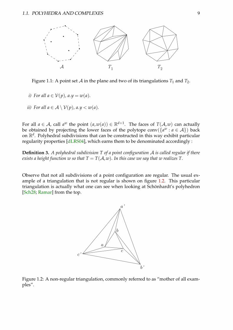
We call triangulation of a point configuration A any polyhedral subdivision T of Awhose faces are simplices. As an example, figure 1.1 shows a point configuration andtwo of its triangulations.
A face f of T is called interior if it intersects the relative interior of dom(T). For aface s of a triangulation T, we call star of s in T the set {p ∈ T : conv(s ∪ p) ∈ T} andlink of s in T the set {p ∈ T : conv(s ∪ p) ∈ T, s 6⊂ p}. Let A be a point configurationof Rd. A height function on A is any function w : A → R. Height functions induceparticular polyhedral subdivisions of their underlying point configurations accordingto the following proposition :
Proposition 2. Let A be a point configuration of Rd and w a height function on A. There isa unique polyhedral subdivision T(A, w) of A so that for all p ∈ T(A, w), there exists y ∈ Rd
satisfying the following two statements :
1.1. POLYHEDRA AND COMPLEXES 9
A T1 T2
Figure 1.1: A point set A in the plane and two of its triangulations T1 and T2.
i) For all a ∈ V(p), a.y = w(a).
ii) For all a ∈ A \ V(p), a.y < w(a).
For all a ∈ A, call aw the point (a, w(a)) ∈ Rd+1. The faces of T(A, w) can actuallybe obtained by projecting the lower faces of the polytope conv({aw : a ∈ A}) backon Rd. Polyhedral subdivisions that can be constructed in this way exhibit particularregularity properties [dLRS04], which earns them to be denominated accordingly :
Definition 3. A polyhedral subdivision T of a point configuration A is called regular if thereexists a height function w so that T = T(A, w). In this case we say that w realizes T.
Observe that not all subdivisions of a point configuration are regular. The usual ex-ample of a triangulation that is not regular is shown on figure 1.2. This particulartriangulation is actually what one can see when looking at Schönhardt’s polyhedron[Sch28; Ramar] from the top.
a
b
c
b'
c'
a'
Figure 1.2: A non-regular triangulation, commonly referred to as “mother of all exam-ples”.
10 CHAPTER 1. MATHEMATICAL PRELIMINARIES
1.2 On the flip-graph of regular triangulations
In the method described in chapter 3, a way to regularize triangulations will be needed.The problem can be stated as follows. Let (Si)1≤i≤n be a set of spheres with centers(Ri)1≤i≤n. Provided a triangulation T of the point configuration A= {xi : 1≤ i ≤ n} isknown, one needs to transform T into the weighted Delaunay triangulation generatedby (Si)1≤i≤n at the lowest possible cost.
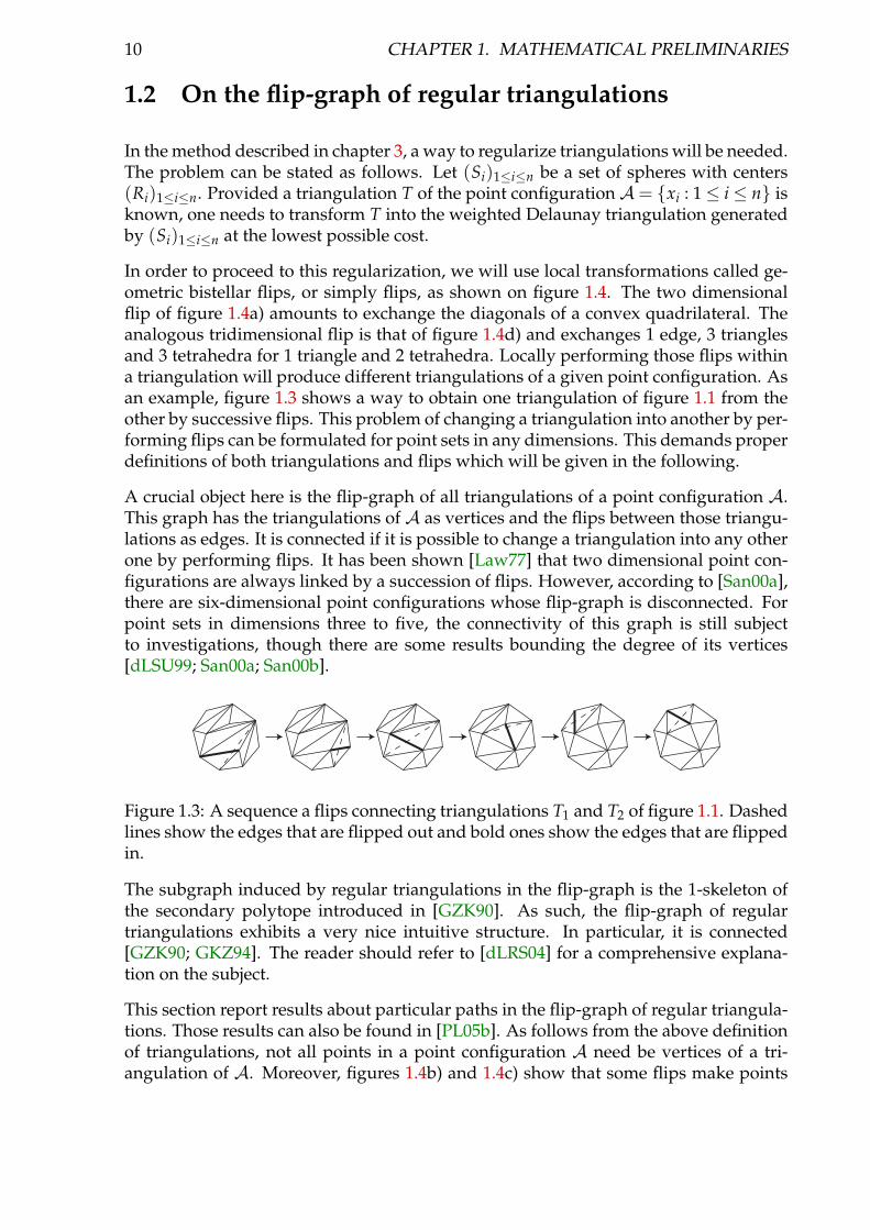
In order to proceed to this regularization, we will use local transformations called ge-ometric bistellar flips, or simply flips, as shown on figure 1.4. The two dimensionalflip of figure 1.4a) amounts to exchange the diagonals of a convex quadrilateral. Theanalogous tridimensional flip is that of figure 1.4d) and exchanges 1 edge, 3 trianglesand 3 tetrahedra for 1 triangle and 2 tetrahedra. Locally performing those flips withina triangulation will produce different triangulations of a given point configuration. Asan example, figure 1.3 shows a way to obtain one triangulation of figure 1.1 from theother by successive flips. This problem of changing a triangulation into another by per-forming flips can be formulated for point sets in any dimensions. This demands properdefinitions of both triangulations and flips which will be given in the following.
A crucial object here is the flip-graph of all triangulations of a point configuration A.This graph has the triangulations of A as vertices and the flips between those triangu-lations as edges. It is connected if it is possible to change a triangulation into any otherone by performing flips. It has been shown [Law77] that two dimensional point con-figurations are always linked by a succession of flips. However, according to [San00a],there are six-dimensional point configurations whose flip-graph is disconnected. Forpoint sets in dimensions three to five, the connectivity of this graph is still subjectto investigations, though there are some results bounding the degree of its vertices[dLSU99; San00a; San00b].
Figure 1.3: A sequence a flips connecting triangulations T1 and T2 of figure 1.1. Dashedlines show the edges that are flipped out and bold ones show the edges that are flippedin.
The subgraph induced by regular triangulations in the flip-graph is the 1-skeleton ofthe secondary polytope introduced in [GZK90]. As such, the flip-graph of regulartriangulations exhibits a very nice intuitive structure. In particular, it is connected[GZK90; GKZ94]. The reader should refer to [dLRS04] for a comprehensive explana-tion on the subject.
This section report results about particular paths in the flip-graph of regular triangula-tions. Those results can also be found in [PL05b]. As follows from the above definitionof triangulations, not all points in a point configuration A need be vertices of a tri-angulation of A. Moreover, figures 1.4b) and 1.4c) show that some flips make points

1.2. ON THE FLIP-GRAPH OF REGULAR TRIANGULATIONS 11
appear or disappear in the triangulation. It is possible to flip a triangulation of a pointconfiguration to another by going through triangulations whose vertex sets are quitedifferent. Indeed, the only points strictly required as vertices for any triangulation ofA are the extreme points of the convex hull of A. Theorem 3 states that when flippinga regular triangulation into another whose vertex set is a subset of the first, it is possi-ble to keep monotone the number of vertices of the triangulations met in the process.As a corollary, the flip-graph of regular triangulations whose vertex sets are identicalis connected. This connectivity property actually reveals crucial for our contact detec-tion method (see chapter 3), where the vertices of the triangulation represent particles.Deleting those vertices while a simulation proccesses is therefore inappropriate in thiscase.
1.2.1 Geometric bistellar operations
The notion of flip has been illustrated in the introduction by the two dimensional exam-ple of figure 1.4a) that consists in exchanging the diagonals of a convex quadrilateral.Observe that the flip shown in figure 1.4b) exhibits a different structure, as it makes avertex appear or disappear. Degenerate cases may occur as well, like the flip of figure1.4c) where five vertices are involved, three of them being aligned, and one of them ap-pearing or disappearing depending on the triangulation in which the flip is performed.The simplest three-dimensional flip, shown in figure 1.4d) consists in exchanging twotetrahedra and a triangle for three tetrahedra, three triangles and an edge. Of course,flips analogous to those of figures 1.4b) and 1.4c) also exist in three dimensions. In thissection, we give a definition in any dimension of those geometric bistellar operations,thus gathering the flips of figure 1.4 into one unique description.
a
b
c
d
a)
a
b
c
d
da
b
c
b)
a
b
c c)
a
b
c
d
a
b
c
d
e
a
b
c
d
a
b
c
d
ea
b
c
d
d)
e
e
Figure 1.4: Some flips
We call circuit any minimal affinely dependent subset Z of Rd and for a point config-uration A, we denote by CA the set of all circuits Z ⊂ A. The set {a, b, c, d} is a circuitin figures 1.4a) and 1.4b) and {b, d, e} is one in figure 1.4c). A circuit admits exactly

12 CHAPTER 1. MATHEMATICAL PRELIMINARIES
two triangulations. This comes from the existence of the so-called Radon partition ofcircuits, according to the following theorem :
Theorem 1. Let Z ⊂ Rd be a circuit. There exists a unique partition (Z−, Z+) of Z so thatconv(Z−) ∩ conv(Z+) 6= ∅.
Let (Z−, Z+) be the Radon partition of a circuit Z and consider the two subsets of PZdefined by T− = {s ∈ PZ : Z− 6⊂ s} and T+ = {s ∈ PZ : Z+ 6⊂ s}. Every simplex inPZ either belongs to T− or to T+. Moreover, one can check that both T− and T+ aretriangulations by using the unicity of (Z−, Z+) as a partition of Z so that conv(Z−) ∩conv(Z+) 6= ∅. This proves that Z admits T− and T+ as its only two triangulations.While knowing that a circuit admits exactly two triangulations is not strictly requiredto proceed with the definition of flips, it helps to understand the structure of circuits,which are the minimal point configurations admitting more than one triangulation.
Definition 4. Let T be a triangulation of a point configuration A. Suppose the two followingstatements are satisfied by some circuit Z ⊂A :
i) Some triangulation T− of Z is a subcomplex of T.
ii) All cells of T− have the same link L in T.
Then, we say that Z is a flippable circuit in T. Moreover, a triangulation T′ ofA can be obtainedby replacing T− ? L by T+ ? L in T. This operation is called a geometric bistellar flip and wesay that T and T′ are geometric bistellar neighbors.
Observe on figures 1.4a) and 1.4b) that {a, b, c, d} are flippable circuits, the link L statedin ii) being empty. On figure 1.4c), however, {b, d, e} is a flippable circuit with L ={a, c}. Actually, statement ii) will only be useful when the circuit to be flipped is notfull-dimensional, the flip itself being degenerate as that of figure 1.4c).
1.2.2 Monotone connectivity of the graph of regular triangulations
Let A be a configuration of n points in Rd. Since the space of height functions on A isa vector space of dimension n, we will identify it with Rn from now on. For a givenregular polyhedral subdivision T of A, we denote by CA(T) the set {w ∈ Rn : T =T(A, w)} of all height functions realizing T. We further denote by CA the collection ofthe CA(T) over all regular polyhedral subdivisions T of A. The following propositionis proven in [GZK90] :
Proposition 3. The set CA is a complete polyhedral fan. Moreover, for a regular polyhedralsubdivision T of A, the polyhedral cone CA(T) is full-dimensional if and only if T is a trian-gulation.
The fan CA is called secondary fan of A, and for a regular polyhedral subdivision T ofA, the cone CA(T) is referred to as secondary cone of T. The following theorem states acrucial property of the secondary fan. Its proof can be found in [dLRS04] :

1.2. ON THE FLIP-GRAPH OF REGULAR TRIANGULATIONS 13
Theorem 2. Two regular triangulations T and T′ of a point configuration A are geometricbistellar neighbors if and only if their secondary cones share a common facet.
To these results, we now add another one which will be used in the proof of theorem3 to make sure that the sequence of triangulations we search for is monotone. For anypoint a ∈ A we call KA(a) the set {w ∈ Rn : a ∈ T(A, w)} of all height functions whoseinduced polyhedral subdivisions of A admit a as a vertex.
Lemma 1. Let A⊂ Rd be a point configuration. For all a ∈ A, the set KA(a) is convex.
Proof. Let w and w′ be two elements of KA(a) and λ an element of [0, 1]. We will showthat w′′ = λw + (1− λ)w′ still belongs toKA(a). According to proposition 2, there existtwo vectors y and y′ in Rd so that y.a = w(a) and y′.a = w′(a) while for all v ∈ A \ {a},y.v < w(v) and y′.v < w′(v). Call y′′ the vector λy + (1 − λ)y′ ∈ Rd. By linearity ofthe scalar product, one finds y′′.a = w′′(a) while for all v ∈ A \ {a}, y′′.v < w′′(v). Itfollows from proposition 2 that a is a vertex of T(A, w′′), which proves that KA(a) isconvex.
Actually, for a ∈A the setKA(a) is a full-dimensional open polyhedral cone. However,we only need its convexity here which explains the way lemma 1 has been stated. Weare now ready to prove our main result :
Theorem 3. LetA⊂Rd be a point configuration. Let T and T′ be regular triangulations ofAso that V(T′) ⊂ V(T). Then there exists a finite sequence T0, ..., Tn of regular triangulationsof A so that T = T0, T′ = Tn and for any i ∈ {0, ..., n− 1},
i) Ti and Ti+1 are geometric bistellar neighbors.
ii) VTi+1 ⊂ VTi .
Proof. Observe that any regular triangulation of V(T) is a regular triangulation of A.We can therefore assume without loss of generality that A = V(T).
According to proposition 3, the cones CA(T) and CA(T′) are full dimensional and assuch, their interiors are not empty. Observe that it is then possible to choose two heightfunctions w and w′ in the interiors of CA(T) and CA(T′) respectively so that all faces ofCA intercepted by segment conv(w, w′) either are facets or cells. Let (w, w′) be such apair of height functions.
We denote by T0, ...., Tn the sequence of regular triangulations of A so that CA(T0), ...,CA(Tn) are those cells of CA successively met when conv(w, w′) is traversed from w tow′. Observe that T0 = T and Tn = T′. For any i ∈ {0, ..., n− 1}, according to the way(w, w′) was chosen, the secondary cones CA(Ti) and CA(Ti+1) share a common facet.Theorem 2 then makes sure that triangulations T0, ...., Tn satisfy statement i).
For any i ∈ {0, ..., n− 1}, let a be a vertex of Ti+1. Since a is a vertex of T0 as well, theconvexity of {w ∈ Rn : a ∈ T(A, w)} provided by lemma 1 implies that a is a vertex ofTi. Triangulations T0, ...., Tn then satisfy statement ii) and the theorem is proven.

14 CHAPTER 1. MATHEMATICAL PRELIMINARIES
While theorem 3 is the main result of this section, we now state a corollary that may bemore appealing for it asserts the connectivity of some subgraphs of the flip-graph ofregular triangulations. This result is particularly interesting for practical applications,and in particular for the contact detection method described in chapter 3. Indeed, thevertices of a triangulation represent the particles, therefore deleting them in the courseof the simulation is inappropriate.
Corollary 1. Let A be a point configuration in Rd. The flip-graph of those regular triangula-tions of A that share A as a common vertex set is connected.
1.3 Weighted Delaunay triangulations and power diagrams
Previous sections introduce regular triangulations by using height functions. This sec-tion presents another way to look at that particular class of triangulations, using theformalism of power diagrams. This formalism makes it possible to derive some of theirproperties that will be used in chapter 3, such as their ability to evaluate distances be-tween neighbors among an assembly of spheres.
Assume (Si)1≤i≤n is an assembly of n spheres in Rd whith centers (xi)1≤i≤n and radii(Ri)1≤i≤n. Consider the power distance πi to the sphere Si defined on Rd by :
πi : Rd → R,x 7→ ‖x− xi‖2 − R2
i .(1.1)
When x lies outside Si, πi(x) is the square of the distance between point x and sphereSi measured along a line tangent to Si, as figure 1.5 suggests. Now, call pi the subsetof Rd constituted by points x so that for all j 6= i, πi(x) ≤ π j(x). The (pi)1≤i≤n happento be polyhedra which are the cells of a polyhedral complex C called power diagram orsometimes Laguerre complex generated by the spheres S1, ..., Sn. Such a power diagramis shown on figure 1.6 in two dimensions. More details about power diagrams, andparticularly proofs of above assertions can be found in [BY95].
The power diagram C generated by spheres (Si)1≤i≤n happens to be a geometrical dualof a particular regular triangulation of the point configuration A = {xi : 1 ≤ i ≤ n}.Indeed, for each face p of C((Si)1≤i≤n), consider the polyhedron p∗ whose vertices arethose xi so that p is a face of Ci. The set {p∗ : p ∈ C} is then a polyhedral subdivisionof A (see [BY95] for proofs). Moreover, this subdivision is realized by the followingheight function :
w :A → R,xi 7→ ‖xi‖2 − R2
i .(1.2)
Thus, {p∗ : p ∈ C} is a regular subdivision of A. When w is in general position,{p∗ : p ∈ C} is a regular triangulation called weighted Delaunay triangulation generated

1.3. WEIGHTED DELAUNAY TRIANGULATIONS AND POWER DIAGRAMS 15
x
x π (x)ii
Ri
Si kx -xk i
Figure 1.5: The power distance of point x with respect to sphere Si.
by the spheres (Si)1≤i≤n. We say that the spheres (Si)1≤i≤n are in general position when-ever the height function (1.2) they provide is in general position. Figure 1.6 depicts theweighted Delaunay triangulation corresponding to the power diagram already men-tioned above in two dimensions.
We say that two spheres Si and S j are less than orthogonal if ‖x j − xi‖2 > R2i + R2
j . Thiscondition, forbids spheres Si and S j to overlap too much. More precisely, their overlapshould be strictly lower than in the case where they are orthogonal. We call orthogonal-ity condition the following condition on the spheres (Si)1≤i≤n :
∀ (i, j) ∈ {1, ..., n}2, i 6= j⇒ ‖x j − xi‖2 > R2i + R2
j . (1.3)
Whenever this condition is satisfied, the weighted Delaunay triangulation generatedby the spheres (Si)1≤i≤n is able to provide all the intersecting pairs among those spheres,according to the following theorem :
Theorem 4. Let (Si)1≤i≤n be a set of spheres in general position that satisfy the orthogonalitycondition (1.3). For any i 6= j, if spheres Si and S j intersect then conv({xi, x j}) is a face of theweighted Delaunay triangulation generated by (Si)1≤i≤n.
Proof. Suppose that Si and S j intersect and consider k ∈ {1, ..., n} \ {i, j}. Call x thepoint in conv({xi, x j}) so that πi(x) = π j(x). As the pair (Si, Sk) is less than orthogonal,we have ‖xk − xi‖2 > R2
i + R2k . Introducing x in the left hand side of this inequation
and developing the scalar product, one finds πk(x) + πi(x) > 2(xk − x).(xi − x). Thesame arguments hold for the pair (S j, Sk) and we obtain the following system :
{πi(x) + πk(x) > 2(xk − x).(xi − x)π j(x) + πk(x) > 2(xk − x).(x j − x) (1.4)
Since spheres Si and S j intersect, x lies inside both of them, which implies that πi(x)≤ 0and π j(x) ≤ 0. From inequations (1.4), πk(x) is then strictly greater than both 2(xk −

16 CHAPTER 1. MATHEMATICAL PRELIMINARIES
Figure 1.6: The weighted Delaunay triangulation (solid lines) and the power diagram(dashed lines) generated by a set of circles in the plane.
x).(xi − x) and 2(xk − x).(x j − x). Since those two quantities have opposite signs, weobtain πk(x) > 0. As a consequence, πk(x) is strictly greater than both πi(x) and π j(x),and this for all k 6∈ {i, j}. This means that x lies in the relative interior of a commonfacet of Ci and C j. According to the way the weighted Delaunay triangulation is de-duced from the power diagram, conv({xi, x j}) then is a face of the weighted Delaunaytriangulation generated by spheres (Si)1≤i≤n.
Assuming that the spheres (Si)1≤i≤n are spherical grains constituting a granular medium,they should physically satisfy the orthogonality condition and theorem 4 makes surethat all interparticle contacts will be found among the edges of the weighted Delaunaytriangulation they generate. This property has already been used in the theses of D.Müller [Mül96a] and J.-A. Ferrez [Fer01] (see also [FL02]) in order to detect contactsbetween spherical grains in two and three dimensions respectively.
Theorem 4 can be generalized by appropriately relaxing the orthogonality condition.

1.3. WEIGHTED DELAUNAY TRIANGULATIONS AND POWER DIAGRAMS 17
Consider the following condition on spheres (Si)1≤i≤n, called overlapping condition :
∀ (i, j) ∈ {1, ..., n}2, i 6= j⇒ ‖x j − xi‖2 > |R2j − R2
i |. (1.5)
Observe that if spheres (Si)1≤i≤n satisfy this overlapping condition, all the xi are ver-tices of the weighted Delaunay triangulation they generate. Assume spheres (Si)1≤i≤nsatisfy the overlapping condition, and let I be a subset of {1, ..., n}. We say that spheres(Si)i∈I are congruous if they satisfy the following statement :
∀ (i, j) ∈ I × I,‖x j − xi‖2 > R2i + R2
j , (1.6)
where I = {1, ..., n} \ I. The weighted Delaunay triangulation generated by (Si)1≤i≤ncan be used to detect whether two congruous sets of spheres overlap, according to thefollowing theorem :
Theorem 5. Let (Si)1≤i≤n be a set of spheres in general position that satisfy the overlappingcondition (1.5) and let (Si)i∈I and (Si)i∈J be two distinct congruous subsets of (Si)1≤i≤n. If∪i∈Iconv(Si) and ∪ j∈Jconv(S j) intersect, there exist i ∈ I and j ∈ J so that conv({xi, x j}) isa face of the weighted Delaunay triangulation generated by (Si)1≤i≤n.
Proof. Among those pairs (i, j) ∈ I × J for which conv(Si) and conv(S j) intersect, takeone that minimizes ‖x j − xi‖2 − R2
i − R2j . Call x the point in conv({xi, x j}) so that
πi(x) = π j(x). Let k ∈ {1, ..., n} \ {i, j}.
If k 6∈ I ∩ J, pairs (Si, Sk) and (S j, Sk) are less than orthogonal and using the samearguments as in the proof of theorem , we find that πk(x) is strictly greater than bothπi(x) and π j(x).
Now assume that k is in I∩ J. The situation is symmetric in I and J and we can thereforeassume without loss of generality that k ∈ J. Using (1.1), we have :
πk(xi)− π j(xi) = ‖xk − xi‖2 − R2k − R2
i − ‖x j − xi‖2 + R2j + R2
i . (1.7)
From the way (i, j) was chosen, ‖x j − xi‖2 − R2i − R2
j is not greater than ‖xk − xi‖2 −R2
i − R2k and equation (1.7) gives πk(xi) ≤ π j(xi), that is x j lies in the affine half-space
E defined by πk − π j ≥ 0..
Now observe that the overlapping condition (1.5) implies πk(x j) > π j(x j). Point xktherefore lies in the interior of E and by convexity of E, so does the relative interior ofthe line segment conv({x j, xk}). In particular, x lies in the interior of E which readsπk(x) > π j(x).
We have shown that for all k ∈ {1, ..., n} \ {i, j}, πk(x) is strictly greater than both πi(x)and π j(x). Point x therefore lies in the relative interior of a common facet of Ci and C j.According to the way the weighted Delaunay triangulation is deduced from the powerdiagram, conv({xi, x j}) is a face of the weighted Delaunay triangulation generated byspheres (Si)1≤i≤n.

18 CHAPTER 1. MATHEMATICAL PRELIMINARIES
Theorem 5 will be used in chapter 3 for the detection of contacts between non-sphericalgrains. We will now give a local characterization of weighted Delaunay triangulationsas well as a property that will turn out to be crucial for the regularization algorithm ofsection 3.3.
Assume (Si)1≤i≤n is an assembly of n spheres in general position in Rd with centers(xi)1≤i≤n and radii (Ri)1≤i≤n and let T be a triangulation of the point configuration{xi : 1 ≤ i ≤ n}. Let f be an interior facet of T, and (a, b) the pair of vertices of T sothat conv({a} ∪ f ) and conv({b} ∪ f ) are maximal faces of T. Let x be the center of thecircumsphere S of conv({b} ∪ f ) and R its radius. According to (1.1), the power of awith respect to sphere S reads ‖x− a‖2 − R2. We say that f is legal if ‖x− a‖2 − R2 > 0and illegal if ‖x − a‖2 − R2 < 0. Since spheres (Si)1≤i≤n are in general positions, thecase ‖x − a‖2 = R2 does not occur. We say that a facet f is flippable if its vertex settogether with {a, b} is a flippable circuit. The following theorem is a classical result ofcomputational geometry and its proof can be found in [BY95] or in [ES96]:
Theorem 6. A triangulation of {xi : 1 ≤ i ≤ n} is the weighted Delaunay triangulation Dgenerated by spheres (Si)1≤i≤n if and only if its vertex set contains that of D and all its interiorfacets are legal.
This theorem provides a way to check whether a triangulation is the weighted De-launay triangulation generated by spheres (Si)1≤i≤n by performing one local test foreach of its interior facets. Intuition suggests that we can obtain the weighted Delaunaytriangulation generated by spheres (Si)1≤i≤n by successively flipping illegal flippablefacets in a triangulation T. We can formulate the following theorem:
Theorem 7. Any triangulation of {xi : 1≤ i≤ n} can be flipped to a triangulation that admitsno facet simultaneously illegal and flippable.
Proof. We will only sketch the proof of theorem 7 here. Let T be a triangulation of{xi : 1≤ i ≤ n}. Observe that lifting the vertices of T to Rd+1 using the height function(1.2) allows to represent T as a polyhedral surface Σ in Rd+1. Assume that T admitsillegal flippable facets. It turns out that the illegal facets of T correspond to the non-convexities of Σ. Therefore if f is an illegal flippable facet of T, flipping it will producea triangulation T′ whose associated polyhedral surface Σ′ lies strictly below Σ (whichcan also be formulated as : the volume below Σ′ is strictly smaller than the volumebelow Σ). By strictly below, we mean that Σ′ is below Σ, while it is not identical toΣ. This means that it is impossible to cycle by successively flipping illegal flippablefacets. Since the number of triangulations of {xi : 1≤ i≤ n} is finite, a triangulation thatadmits no facet simultaneously illegal and flippable will eventually be reached.
Observe that the triangulation T′ eventually reached by successively flipping illegalflippable facets from a triangulation T of {xi : 1 ≤ i ≤ n} may not be the weighted De-launay triangulation D generated by spheres (Si)1≤i≤n. It can be proven that whenflipping illegal flippable facets, vertices of the weighted Delaunay triangulation gen-erated by spheres (Si)1≤i≤n will never appear or disappear. Therefore if the vertex setof T does not contain that of D, triangulation T′ cannot be equal to D. If VD ⊂ VT thenVD ⊂ VT′ as well but T′ still may admit illegal facets. According to theorem 6, T′ willbe equal to D if and only if VD ⊂ VT and T′ has no illegal facet.

Chapter 2
The Distinct Element Method
The distinct element method is widely used to simulate phenomena involving grains.It allows to simulate on a computer the time evolution of a set of particles submitted toforces such as interparticle contact forces and gravity. Suppose P1, ..., Pk are particles ina three dimensional space evolving between a time t0 and a time t f . What the distinctelement method needs to proceed are the spacial configuration of P1, ..., Pk a time t0and a way to compute the forces acting on P1, ..., Pk at a time t ∈ [t0, t f ], from the onlyknowledge of their spacial configuration. Several methods can be used to integrate themotion of the particles. Here, we consider the simplest one: Euler’s integration scheme.A time step ∆t =
t f−t0N is used to discretize [t0, t f ] in a number N ∈N∗ of time intervals
[t0 + i∆t, t0 + (i + 1)∆t] for i ∈ {0, ..., N − 1}. This method further assumes that all theforces the particles are submitted to are constant within each of those time intervals ofduration ∆t. Therefore, by integrating the motion equations, the spacial configurationof P1, ..., Pk at time t0 + (i + 1)∆t is easily deducible from that at time t0 + i∆t. Theoverall process can be summarized as follows :
1. From the configuration of P1, ..., Pk at time t0 + i∆t, compute the forces acting onP1, ..., Pk.
2. Assuming the forces acting on the particles are constant within [t0 + i∆t, t0 +(i + 1)∆t], solve the motion equation for each individual particle inside the timeinterval [t0 + i∆t, t0 + (i + 1)∆t] and find its position at time t0 + (i + 1)∆t.
3. set i + 1→ i and return to 1.
Though this general description gives an overall idea of the DEM framework, someof its key components need to be further described in order for any implementationto be possible. In particular, a way to compute the forces acting on the particles fromthe sole knowledge of their spacial configuration still has to be practically formulated.This requires to model contacts between particles together with contact forces, but alsothe very shapes of the particles. These few issues are discussed in the remaining of thischapter.

20 CHAPTER 2. THE DISTINCT ELEMENT METHOD
2.1 A model for particle shapes
Let S be the pointwise union of a finite number of simplices of R3 and r > 0 a realnumber. The particle Π(S, r) consists of the points x ∈ R3 whose euclidean distance toS is not greater than r. This amounts to taking the Minkowski sum of the set S withthe ball of R3 of radius r centered at point 0. The set S is called skeleton of Π(S, r) andthe real number r is called radius of Π(S, r). If S is a point, Π(S, r) is the ball of R3 ofradius r centered at point S. If S is a line segment, Π(S, r) is called spherosegment, ormore usually spherocylinder. If S is a triangle, Π(S, r) is called spherotriangle and if it is atetrahedron, Π(S, r) is called spherotetrahedron. Balls, spherosegments, spherotrianglesand spherotetrahedra are what we call spherosimplices (figure 2.1). When S is a poly-hedron, Π(S, r) is a spheropolyhedron. Let s1, ..., sk be the simplices whose pointwiseunion is the set S. The particle Π(S, r) is then exactly the union ∪k
i=1Π(si, r) of basicspherosimplices.
Figure 2.1: The Minkowski sums of a sphere with a line segment, a triangle and atetrahedron. These particular shapes, called spherosimplices are some of the basicobjects constituting the general particle model used in this work.
Actually, some skeletons may contain superfluous information as sketched in figure2.2. Indeed, if p is a point in S whose distance to the boundary of Π(S \ {p}, r) isstrictly greater than r, then Π(S, r) = Π(S \ {p}, r). Using particles so that the distanceof any point p ∈ S to the boundary of Π(S \ {p}, r) is r will simplify their handling,avoiding useless calculations due to unnecessarily complex skeletons.
Observe that this geometrical description of the particle shapes assumes that they havea given position in space. Upon introduction of the time variable, the particles will beallowed to move accordingly to the rules underlying to the DEM framework. Theparticles will therefore be allowed to translate and rotate as a response to the physicalconstraints they will be subject to, but their shapes will remain unchanged. It followsthat the skeleton S of a particle will be a function S(t) of time whose values will bededucible one from the other by a translation and a rotation. While P will then be thefunction of time P(t) = Π(S(t), r), P and its incarnation P(t) at different times t will beused indifferently whenever t does not need to be specified.

2.1. A MODEL FOR PARTICLE SHAPES 21
r
P
S
B
σ
x y
z
r
σ
x y
z
+ =
Figure 2.2: A two-dimensional particle P = Π(S, r) obtained as the Minkowski sum ofa set of simplices S with a ball of radius r. The skeleton S contains a line segment σ
whose Minkowski sum Π(σ , r) with the same ball is sketched as a dashed line. The setΠ(σ , r) strictly lies in the interior of P and therefore removing σ from S will not changeP
2.1.1 Contacts and overlaps between particles
Two particles P1 and P2 are said to be in contact if they overlap, that is if P1 ∩ P2 6= ∅.This simple notion may seem shockingly unrealistic as two distinct solids will neversimultaneously occupy the same portion of space. However, this model does have aphysical interpretation and turns out to be very convenient for quantifying the geo-metrical properties of a contact when attempting to decide of a model for its physicalbehaviour.
Indeed, two particles experiencing a contact slightly deform at the contact point. In-stead of using an explicit model for the deformation of the grain shapes, which woulddemand forbiddingly large computational efforts anyway, the shapes of the particleswill remain unchanged and the deformation of the contact area will be modeled by thean overlapping between the particles, as sketched in figure 2.3.
The idea is that the relative position between the two undeformed particles in contactshould be that they would have if they could deform. The amplitude of the overlapwill then model the amount of deformation deformable particles would show in thesame contact conditions. Observe that from the definition of a particle, two particlesP1 = Π(S1, r1) and P2 = Π(S2, r2) overlap if and only if there exist two points x1 ∈S1 and x2 ∈ S2 so that ‖x1 − x2‖ < r1 + r2. If two particles P1 and P2 are in contactand at least one of them is non-convex, the overlapping area P1 ∩ P2 is not necessarilyconnected, that is P1 and P2 have several contacting areas as shown on figure 2.4.
This case shows that the above definition of a contact needs to be further refined. Tothis end, advantage can be taken of the way the particles have been defined and thefollowing distance function can be introduced :

22 CHAPTER 2. THE DISTINCT ELEMENT METHOD
P1
contact overlap
P2
P1
P2v22
v1
Figure 2.3: The deformation at the contact point is modeled by an overlapping of un-deformed particles. The dashed line on the right-hand side sketches the deformationthe contacting particles would experience if they were deformable
P1
P2
S1
S2
r1
r2
Figure 2.4: Two particles experiencing several simultaneous contacts because one ofthem is non-convex.
d : S1 × S2 → R+
(y1, y2) 7→ ‖y2 − y1‖(2.1)
Contacts between P1 and P2 will each be identified with a local minimum of functiond. This function therefore separates the individual contact areas. Still not all amongthe local minima of function d will correspond to a contact. As an example, figure 2.5shows a local minimum of function d where no overlapping occurs between P1 and P2.It follows that the local minima (x1, x2) of function d such that r1 + r2 − ‖x2 − x1‖ < 0will not provide any contact point between P1 and P2.
Given a local minimum (x1, x2) of function d, the distance between point x1 and theboundary of P1 along segment x1x2 reads :
2.1. A MODEL FOR PARTICLE SHAPES 23
S1
S2
P2
P1
r2
r1
x2
x1
Figure 2.5: Some local minima of function d may not correpond to overlapping areas
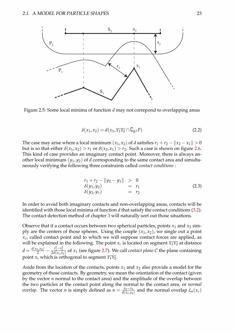
δ(x1, x2) = d(x1, x1x2 ∩ {R3 P) (2.2)
The case may arise where a local minimum (x1, x2) of d satisfies r1 + r2−‖x2− x1‖> 0but is so that either δ(x1, x2) > r1 or δ(x2, x1) > r2. Such a case is shown on figure 2.6.This kind of case provides an imaginary contact point. Moreover, there is always an-other local minimum (y1, y2) of d corresponding to the same contact area and simulta-neously verifying the following three constraints called contact conditions :
r1 + r2 − ‖y2 − y1‖ > 0δ(y1, y2) = r1δ(y2, y1) = r2
(2.3)
In order to avoid both imaginary contacts and non-overlapping areas, contacts will beidentified with those local minima of function d that satisfy the contact conditions (3.2).The contact detection method of chapter 3 will naturally sort out those situations.
Observe that if a contact occurs between two spherical particles, points x1 and x2 sim-ply are the centers of those spheres. Using the couple (x1, x2), we single out a pointxc, called contact point and to which we will suppose contact forces are applied, aswill be explained in the following. The point xc is located on segment x1x2 at distance
d = d(x1 ,x2)2 − r2
1−r22
2d(x1 ,x2)of x1 (see figure 2.7). We call contact plane C the plane containing
point xc which is orthogonal to segment x1x2.
Aside from the location of the contacts, points x1 and x2 also provide a model for thegeometry of those contacts. By geometry, we mean the orientation of the contact (givenby the vector n normal to the contact area) and the amplitude of the overlap betweenthe two particles at the contact point along the normal to the contact area, or normaloverlap. The vector n is simply defined as n = x2−x1
d(x1 ,x2)and the normal overlap ξn(xc)
24 CHAPTER 2. THE DISTINCT ELEMENT METHOD
S1
S2
P2
P1
x2
y2
y1x1
xcyc
r2
r1
r2
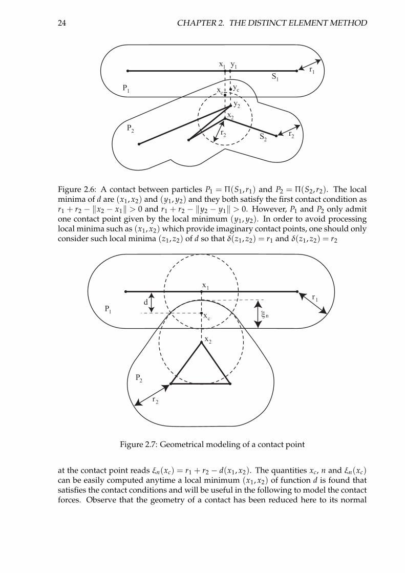
Figure 2.6: A contact between particles P1 = Π(S1, r1) and P2 = Π(S2, r2). The localminima of d are (x1, x2) and (y1, y2) and they both satisfy the first contact condition asr1 + r2 − ‖x2 − x1‖ > 0 and r1 + r2 − ‖y2 − y1‖ > 0. However, P1 and P2 only admitone contact point given by the local minimum (y1, y2). In order to avoid processinglocal minima such as (x1, x2) which provide imaginary contact points, one should onlyconsider such local minima (z1, z2) of d so that δ(z1, z2) = r1 and δ(z1, z2) = r2
d
ξnP1
P2
r2
r1
x2
x1
xc
Figure 2.7: Geometrical modeling of a contact point
at the contact point reads ξn(xc) = r1 + r2 − d(x1, x2). The quantities xc, n and ξn(xc)can be easily computed anytime a local minimum (x1, x2) of function d is found thatsatisfies the contact conditions and will be useful in the following to model the contactforces. Observe that the geometry of a contact has been reduced here to its normal
2.2. CONTACT FORCE MODELING 25
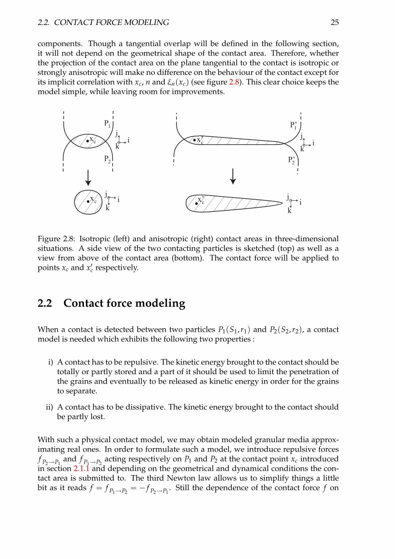
components. Though a tangential overlap will be defined in the following section,it will not depend on the geometrical shape of the contact area. Therefore, whetherthe projection of the contact area on the plane tangential to the contact is isotropic orstrongly anisotropic will make no difference on the behaviour of the contact except forits implicit correlation with xc, n and ξn(xc) (see figure 2.8). This clear choice keeps themodel simple, while leaving room for improvements.
P2 P’2
P’1P1
xc
x’cxc
x’cij
k
ik
j
ij
k
ik
j
Figure 2.8: Isotropic (left) and anisotropic (right) contact areas in three-dimensionalsituations. A side view of the two contacting particles is sketched (top) as well as aview from above of the contact area (bottom). The contact force will be applied topoints xc and x′c respectively.
2.2 Contact force modeling
When a contact is detected between two particles P1(S1, r1) and P2(S2, r2), a contactmodel is needed which exhibits the following two properties :
i) A contact has to be repulsive. The kinetic energy brought to the contact should betotally or partly stored and a part of it should be used to limit the penetration ofthe grains and eventually to be released as kinetic energy in order for the grainsto separate.
ii) A contact has to be dissipative. The kinetic energy brought to the contact shouldbe partly lost.
With such a physical contact model, we may obtain modeled granular media approx-imating real ones. In order to formulate such a model, we introduce repulsive forcesf P2→P1
and f P1→P2acting respectively on P1 and P2 at the contact point xc introduced
in section 2.1.1 and depending on the geometrical and dynamical conditions the con-tact area is submitted to. The third Newton law allows us to simplify things a littlebit as it reads f = f P1→P2
= − f P2→P1. Still the dependence of the contact force f on

26 CHAPTER 2. THE DISTINCT ELEMENT METHOD
the geometrical and dynamical conditions the contact area is submitted to has to bedefined. The geometry of the contact area will be modeled by the overlap ξn and theunitary vector n normal to the contact surface already introduced in section 2.1.1 (seealso figure 2.7), while the relative velocity vr(xc) of P1 and P2 at point xc will model itsdynamics. Calling ω1 and ω2 the spin vectors of P1 and P2, vr(xc) reads :
vr(xc) = x2 − x1 + n ∧ (r1ω1 + r2ω2) (2.4)
One can easily check that the primitive of vr(xc).n which is zero when the contactbegins is exactly ξn. Actually vr(xc) can also be used to define a tangential overlap.Consider the following differential equation :
ξ = (n ∧ n) ∧ξ − vr(xc) (2.5)
We define the vector overlap ξ as the solution of equation (2.5) which is zero when thecontact begins. The normal and tangential overlaps are then given by :
ξn = ξ .nξs = ξ − (ξ .n)n (2.6)
Practically, ξn is given by ξn = r1 + r2 − ‖x2 − x1‖ and under the assumption that thecontact plane does not move much, ξs is given by the following simpler equation :
ξs =∫ t
t0
vr(xc)du, (2.7)
where t0 is the instant the contact begins. The tangential deformation ξs gives the dis-tance between the current position of the contact point and the contact point at instantt0 in a referential attached to the contact plane and accounts for the amount of tan-gential deformation at the contact point in the case of a pure sticky contact. However,a contact may also slip, in which case the tangential deformation either remains con-stant or decreases. A slipping behaviour will be made possible by using Coulombianfriction to limit the magnitude of ξs.
In the molecular dynamics procedure, the contact forces are computed as functions ofthe overlaps ξn and ξs and their time derivatives ξn and ξs :
f = φn(ξn,ξn)n +φs(ξs,ξs) (2.8)
where φs is a vector quantity parallel to the contact plane C. Assuming that the tangen-tial force φs(ξs,ξs) does not already take into account the Coulomb friction, one has toreplace it in (2.8) by :
φCs (ξs,ξs) = min(µφn(ξn,ξn),‖φs(ξs,ξs) ‖)us (2.9)
Where µ is the friction coefficient, and
us =
φs(ξ s ,ξ s)‖φs(ξ s ,ξ s)‖
if φs(ξs,ξs) 6= 0
0 if φs(ξs,ξs) = 0(2.10)
Observe that Coulomb law (2.9) should be implemented by bounding ξs when needed.Here are two examples of force models, which are the most frequently used ones forpractical simulations. We describe those models without the Coulomb friction, whichhas to be added afterwards according to (2.9).

2.3. TUNING MOLECULAR DYNAMICS MODELS WITH REAL EXPERIMENTS 27
• Viscoelastic force : this force, proposed by Cundall and Strack [CS79] is a linearcombination of elastic and viscous terms. Energy is dissipated at the contact pointby the viscous term. We give the linear expression of this force, but non-linearversions have been proposed and investigated (see [KK87])
φn(ξn,ξn) = knξn + cnξn (2.11)
φt(ξ t,ξ t) = ktξ t + ctξ t (2.12)
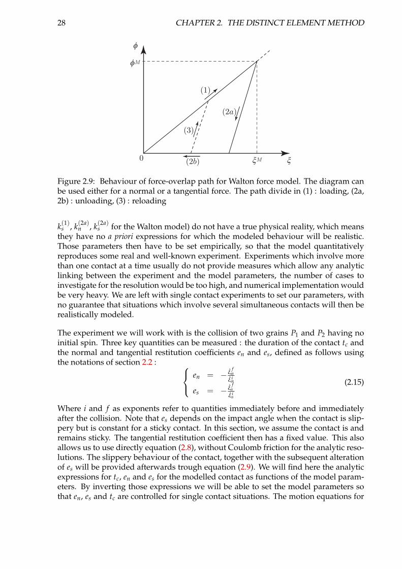
• Walton force : this force, which models the elastoplastic behaviour of the grainsat the contact point was proposed by Walton and Braun [WB86]. The energy isdissipated at a contact as plastic deformation. The loading is assumed elastoplas-tic and the unloading elastic. In either loading and unloading phases, the force istaken as a linear function of the overlap. As the force only depends on the over-lap, the loading-unloading paths obtained with the Walton force model can bedrawn on a force-overlap diagram, as sketched on figure 2.9, left. In order to takeinto account the elastoplastic loading, the loading slope k(1) has to be lower thanthe purely elastic unloading slope k(2a). If a reloading takes place, the force fol-lows a purely elastic slope until it reaches the first loading path (this correspondsto part (3) on the left diagram of figure 2.9). It would have been more realis-tic to model the loading phase as a first purely elastic part followed by a plasticpart, and to take into account the 3/2 exponent given by the Hertz theory for theelastic part, but this simple model contains the overall behaviour of elastoplasticmaterials and is therefore sufficient for a first approximation. The normal forcereads
φn(ξn,ξn) =
{min(k(2a)
n (ξn −ξmn ) +φm
n , k(1)n ξn) (for ξn > 0)
max(k(2a)n (ξn −ξM
n ) +φMn , 0) (for ξn < 0)
(2.13)
where ξMn and φM
n (resp. ξmn and φm
n ) are the values of ξ and φ at the beginning ofthe current unloading (resp. loading) phase (see figure 2.9, left diagram). A sim-ple expression for the tangential Walton force roughly takes on the same featuresas the normal Walton force :
φs(ξs,ξs) =
{min(k(2a)
t (ξs −ξms ) +φm
s , k(1)s ξs)us (for ξs > 0)
max(k(2a)t (ξs −ξM
s ) +φMs , 0)us (for ξs < 0)
(2.14)
Where us is the unit vector defined when ξs 6= 0 by us = ξs/ξs. Both φn and‖ φs ‖ may be drawn as functions of the overlaps (respectively ξn or ξs) on aforce-overlap diagram as the left one of figure 2.9.
2.3 Tuning molecular dynamics models with real experi-ments
The molecular dynamics models described in section 2.2 are technically operational,but the parameters of the force models (kn, ks, cn, cs or the viscoelastic model and k(1)
n ,
28 CHAPTER 2. THE DISTINCT ELEMENT METHOD
Figure 2.9: Behaviour of force-overlap path for Walton force model. The diagram canbe used either for a normal or a tangential force. The path divide in (1) : loading, (2a,2b) : unloading, (3) : reloading
k(1)s , k(2a)
n , k(2a)s for the Walton model) do not have a true physical reality, which means
they have no a priori expressions for which the modeled behaviour will be realistic.Those parameters then have to be set empirically, so that the model quantitativelyreproduces some real and well-known experiment. Experiments which involve morethan one contact at a time usually do not provide measures which allow any analyticlinking between the experiment and the model parameters, the number of cases toinvestigate for the resolution would be too high, and numerical implementation wouldbe very heavy. We are left with single contact experiments to set our parameters, withno guarantee that situations which involve several simultaneous contacts will then berealistically modeled.
The experiment we will work with is the collision of two grains P1 and P2 having noinitial spin. Three key quantities can be measured : the duration of the contact tc andthe normal and tangential restitution coefficients en and es, defined as follows usingthe notations of section 2.2 : en = − ξ
fn
ξ in
es = − ξfs
ξ is
(2.15)
Where i and f as exponents refer to quantities immediately before and immediatelyafter the collision. Note that es depends on the impact angle when the contact is slip-pery but is constant for a sticky contact. In this section, we assume the contact is andremains sticky. The tangential restitution coefficient then has a fixed value. This alsoallows us to use directly equation (2.8), without Coulomb friction for the analytic reso-lutions. The slippery behaviour of the contact, together with the subsequent alterationof es will be provided afterwards trough equation (2.9). We will find here the analyticexpressions for tc, en and es for the modelled contact as functions of the model param-eters. By inverting those expressions we will be able to set the model parameters sothat en, es and tc are controlled for single contact situations. The motion equations for
2.3. TUNING MOLECULAR DYNAMICS MODELS WITH REAL EXPERIMENTS 29
the grains P1 and P2 read : m1 x1 = − fm2 x2 = fI1ω1 = −R1n ∧ fI2ω2 = −R2n ∧ f
(2.16)
As the two grains experience the collision, plane C will not move much, which allowsus to assume n is a constant. (2.5) then simplifies to ξ = −vc and equation (2.4) gives :
ξ = x1 − x2 − n ∧ (r1ω1 + r2ω2) (2.17)
From (2.16) and (2.17) one finds :
ξ = − 1me f f
f − (r2
1I1
+r2
2I2
)φs(ξs,ξs) (2.18)
Where 1/me f f = 1/m1 + 1/m2 As the grains have no initial spin, the centers of thegrains will move in a plane. Calling u⊥ a unit vector normal to that plane, we definea unit vector tangential to the contact by us = n ∧ u⊥. Equation (2.18) then projects onun and ut as follows : ξn = − 1
me f fφn(ξn,ξn)
ξs = −( 1me f f
+ r21
I1+ r2
2I2
)φs(ξs,ξs).us(2.19)
Where ξs = ξs.us. Those differential equations can be solved for ξn and ξs, providedexpressions for φn and φs such as (2.11, 2.12) or (2.13, 2.14). For those two cases, wehave the following solutions :
• Viscoelastic force : from (2.11), (2.12) and (2.19) we find the following set ofdifferential equations : ξn + cn
me f fξn + kn
me f fξn = 0
ξs + cs( 1me f f
+ R21
I1+ R2
2I2
)ξs + ks( 1me f f
+ R21
I1+ R2
2I2
)ξs = 0(2.20)
Solving (2.20) provides expressions for en, es and tc according to (2.15) as func-tions of kn, cn, ks and cs. Inverting those expressions we find :
kn =me f f
t2c
(π2 + ln (en)2)
cn = − 2me f ftc
ln (en)ks = 1
t2c ( 1
me f f+
R21
I1+
R22
I2)(π2 + ln (es)
2)
cs = − 1
tc( 1me f f
+R2
1I1
+R2
2I2
)ln (es)
(2.21)
The set of equations (2.21) allows to derive the contact parameters from the val-ues of en, es and tc for single sticky contacts situations with the viscoelastic forcemodel.
30 CHAPTER 2. THE DISTINCT ELEMENT METHOD
• Walton force : from (2.13), (2.14) and (2.19) we find the following differentialequations :
ξn + k(1)n
me f fξn = 0 (for ξn > 0)
ξs + k(1)s ( 1
me f f+ R2
1I1
+ R22
I2)ξs = 0 (for ξs > 0)
ξn + k(2a)n
me f fξn = k(2a)
n −k(1)n
me f fξM
n (for ξn < 0)
ξs + ( 1me f f
+ R21
I1+ R2
2I2
)k(2a)s ξs
= ( 1me f f
+ R21
I1+ R2
2I2
)(k(2a)s − k(1)
s )ξMs
(for ξs < 0)
(2.22)
Where the quantities ξMn and ξM
s refer to the values of ξn and ξs at the end of theloading phases. Solving (2.22) for solutions with continuous derivatives givesexpressions for en, es and tc according to (2.15) as functions of kn, cn, ks and cs.Inverting those expressions we find :
k(1)n = me f f (
π(1+en)2tc
)2
k(2a)n = me f f (
π(1+en)2tcen
)2
k(1)s = 1
1me f f
+R2
1I1
+R2
2I2
(π(1+es)2tc
)2
k(2a)s = 1
1me f f
+R2
1I1
+R2
2I2
(π(1+es)2tces
)2
(2.23)
Equations (2.23) allow to control the values of en, es and tc for single sticky con-tacts situations with the Walton force model.
By expressing the coefficients of the force models as shown in this section, we knowthat any single sticking contact situation will be realistically modelled. However wehave no guarantee that situations involving several simultaneous contacts will be real-istic.
Chapter 3
A triangulation-based contact detectionmethod
This chapter describes a method based on triangulations for detecting contacts be-tween particles in the DEM framework. This method, first imagined and implementedin the two dimensional case by D. Müller [Mül96a] was extended for tridimensionalspherical particles by J.-A. Ferrez [Fer01]. While D. Müller designed two versions ofthe code, one that could handle spheres and one that could handle polygonal parti-cles, this last version could not be naturally extended to polyhedra due to theoreticallimitations. Indeed, the twodimensional code for polygonal grains uses constrained tri-angulations whose conditions of existence in dimensions higher than two [She05] aretoo restrictive for the algorithm to work. Still an adaptation to the non-spherical par-ticles introduced in chapter 2 of the tridimensional algorithm for spherical particlesis possible, and this is the main subject of this chapter. The first section describes theoriginal method for spheres and the second one its generalization to non-spherical par-ticles. The third section is about the handling of the weighted Delaunay triangulationsused in the contact detection method.
3.1 Spherical particles
We are given a finite number of spheres (Pi)1≤i≤n. Naively testing all the pairs forcontact requires O(n2) time. This becomes prohibitive as n grows, typically in practice103 < n < 105. Others have proposed using spacial decompositions to overcome thisdifficulty [AT87]. Here we use the weighted Delaunay triangulation generated by thefamily spheres (Pi)1≤i≤n as already proposed in [Mül96a; Fer01; FL02]. A long seriesof computational experiments has shown that with this approach, one can reduce thecomputational effort of contact detection from O(n2) to O(n) (see chapter 4).
Observe first that since spheres (Pi)1≤i≤n model physical particles, their mutual over-laps should be rather small. It is therefore justified to assume that orthogonality con-dition (1.3) is satisfied. In this case, theorem 4 makes sure that all interparticle contacts

32 CHAPTER 3. A TRIANGULATION-BASED CONTACT DETECTION METHOD
among spheres (Pi)1≤i≤n are identified by exactly one edge of the weighted Delaunaytriangulation T generated by spheres (Pi)1≤i≤n. Provided this triangulation is known,contact detection can therefore be restricted to those pairs of spheres whose centers arelinked by one of its edges.
Two problems have to be solved in order to make sure this method is efficient. Thebuilding and handling the weighted Delaunay triangulation along with the particle’smotion, will be adressed in section 3.3. The second problem is a nice combinatorial one.Indeed, there exist weighted Delaunay triangulations that admit a quadratic number ofedges [BY95]. In order to know whether or not those quadratic cases arise in practicalsituations, numerical investigations have been conducted whose complexity results arereported in chapter 4.
3.2 Non-spherical particles
In this section, we assume that (Pi)1≤i≤n are particles that are not necessarily spherical,yet their shapes can be described using the model of chapter 2. In order to detectall contacts occuring among those particles, it is possible to generalize the approachdescribed in the preceding section.
Each particle Pi will be associated with a set of spheres Si. We impose Pi to lie inside∪S∈Siconv(S). This restriction will be called covering condition. The weighted Delaunaytriangulation T generated by the set of all covering spheres S = ∪n
i=1Si will be used todetect interparticle contacts, provided that the set of covering spheres S satisfies theoverlapping condition (1.5) and that the spheres Si associated to a particle are congru-ous (that is, satisfy (1.6)). Indeed, if two particles Pi and Pj intercept, sets ∪S∈Siconv(S)and ∪S∈S jconv(S) are bound to intercept as well according to the covering condition.Since the overlapping condition is satisfied and since Si and Si are congruous sets ofspheres, theorem 5 then ensures that there exist Si ∈ Si and S j ∈ S j whose centers arelinked by an edge of T. By successively testing all the edges of T, particle pairs candi-date for contact can thus be detected.
As for the spherical case, this method requires building and updating the weightedDelaunay triangulation. This will be adressed in section 3.3. Of course the problem ofknowing whether or not the number of edges of T is quadratic or not in practical casesremains and one can refer to chapter 4 for numerical complexity tests. Two furtherproblems arise in this non-spherical case. For one, covering each particle with spheresthat satisfy the conditions stated above is required, which will be adressed in section3.2.1. The other problem specific to non-spherical particles is that of finding actualcontact points once a pair of particles has been selected using the triangulation.
Recall from chapter 2 that a contact between particles P = Π(SP, rP) and Q = Π(SQ, rQ)will be identified by a pair (xP, xQ) ∈ SP × SQ chosen among the local minima of func-tion (2.1). If P and Q are two contacting spheres xP and xQ will always be the centersof those spheres. If P and Q are non-spherical particles however, xP and xQ depend onthe relative position of the particles. Moreover if either P or Q are non-convex, there

3.2. NON-SPHERICAL PARTICLES 33
may be several contact points between them, corresponding to different local minimaof function (2.1). Observe that SP and SQ are the pointwise union of basic simplices,that is SP = ∪s∈SP s and SQ = ∪s∈SQ s. For the non-spherical cases, we propose to com-pute the distance between every pair (s, s′) ∈ SP × SQ. The arrangement of simplicesin each skeleton will immediately provide the local minima of function (2.1). Observethat the number of local minima may be infinite (think of parallel spherotriangles). Inthis case, the values for xP and xQ should be chosen as the barycenters of the possiblecandidates for minimization in SP and SQ respectively. Only those local minima thatsatisfy the contact condition will identify actual contacts.
The method proposed above to find the local minima of (2.1) that consists in computingthe distance between all the pairs of simplices constituting SP and SQ proves useful insimple cases, when the skeletons are simplices for example. If the skeletons are consti-tuted by many simplices, though, this process may be unnecessarily time consumingand one can think of better procedures depending on the situation at hand. In thecase of convex skeletons, there only is one contact possible between two particles. Theglobal minimum of function (2.1) then is its only local minimum, if we except the de-generate case of parallel simplices. The problem then amounts to minimize a quadraticfunction under linear constraints which can be done in a variety of ways.
Moreover, theorem 5 only states that a contact will for sure be identified by at least oneedge of T. Depending on the way each particle is covered by its associated spheres, Tmay give information on the localization of contacts. However, if this can be achieved,this has to be properly described and stated as a theorem analogous to theorems 4 and5.
3.2.1 Covering the particles with spheres
The method described in section 3.2 that detects contacts between non-spherical parti-cles requires particles to be covered with spheres. Those spheres are required to satisfythe overlapping condition (1.5) and spheres associated to a particle have to be congru-ous (according to statement (1.6)). In order for contact detection to be possible throughall the simulation process, the set of spheres should keep those properties with themotion of the particles.
Provided those conditions remain satisfied, one can imagine adding covering spheres,deleting others, moving their centers with respect to their associated particles or chang-ing their radii. Using all those degrees of freedom may provide a placement of coveringspheres that is optimal for contact detection purposes. Observe though that findingsuch optimal placements requires that extensive information about the relative posi-tions of the particles be known a priori. While a part of that information may be easilyavailable, making it possible to enhance the quality of contact detection at low cost byproceeding to such modifications, we will not address this subject here and will onlyconsider the coverings so that:
• no sphere is added or deleted,
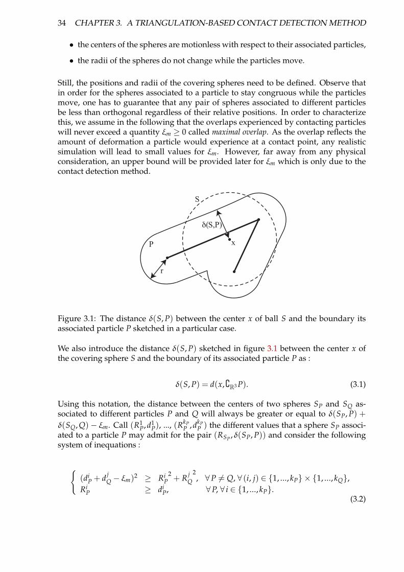
34 CHAPTER 3. A TRIANGULATION-BASED CONTACT DETECTION METHOD
• the centers of the spheres are motionless with respect to their associated particles,
• the radii of the spheres do not change while the particles move.
Still, the positions and radii of the covering spheres need to be defined. Observe thatin order for the spheres associated to a particle to stay congruous while the particlesmove, one has to guarantee that any pair of spheres associated to different particlesbe less than orthogonal regardless of their relative positions. In order to characterizethis, we assume in the following that the overlaps experienced by contacting particleswill never exceed a quantity ξm ≥ 0 called maximal overlap. As the overlap reflects theamount of deformation a particle would experience at a contact point, any realisticsimulation will lead to small values for ξm. However, far away from any physicalconsideration, an upper bound will be provided later for ξm which is only due to thecontact detection method.
r
xP
S
δ(S,P)
Figure 3.1: The distance δ(S, P) between the center x of ball S and the boundary itsassociated particle P sketched in a particular case.
We also introduce the distance δ(S, P) sketched in figure 3.1 between the center x ofthe covering sphere S and the boundary of its associated particle P as :
δ(S, P) = d(x,{R3 P). (3.1)
Using this notation, the distance between the centers of two spheres SP and SQ as-sociated to different particles P and Q will always be greater or equal to δ(SP, P) +δ(SQ, Q)−ξm. Call (R1
P, d1P), ..., (RkP
P , dkPP ) the different values that a sphere SP associ-
ated to a particle P may admit for the pair (RSP ,δ(SP, P)) and consider the followingsystem of inequations :
{(di
P + d jQ −ξm)2 ≥ Ri
P2 + R j
Q2, ∀P 6= Q, ∀ (i, j) ∈ {1, ..., kP} × {1, ..., kQ},
RiP ≥ di
P, ∀P, ∀ i ∈ {1, ..., kP}.(3.2)
3.2. NON-SPHERICAL PARTICLES 35
Following above remarks, admissible solutions of the system (3.2) of inequations pro-vide values for the radii of the covering spheres and distances to the boundary of theirassociated particles that make sure that spheres associated to a particle are congruousindependently of the relative positions of the particles. Moreover, this system requiresthe radii of covering spheres to be greater than the distance to the boundary of theirassociated particle, making it possible to actually cover the particles. While this systemis not linear, fixing the values of the di
P, i ∈ {1, ..., kP} for all particles P will make it so.Choosing in addition kP = 1 for all particles P will provide the following simpler linearsystem, where the exponents have been dropped for obvious reasons :
{R2
P + R2Q ≤ (dP + dQ −ξm)2, ∀P 6= Q,
R2P ≥ d2
P ∀P.(3.3)
Calling n the number of particles, this last system is left with n(n−1)2 + n inequations.
Once an admissible solution for either system (3.2) or system (3.3) has been found, itremains to cover the particles with spheres dimensioned accordingly, keeping in mindthat the overlapping condition (1.5) has to be fulfilled. This constitutes an interestingoptimization problem. It is not necessary to find a set of covering spheres which isminimal. It is sufficient that all particles be covered by their associated spheres whilethe overlapping condition is satisfied. However, in order for the complexity of thecontact detection procedure to remain reasonable, it is of course better to keep the setsof covering spheres as small as possible.
There can be many ways to cover particles with spheres of given sizes. In the following,we propose some simple coverings in particular cases with given particle shapes.
3.2.1.1 Spherocylinders
We assume that all particles to be simulated are spherocylinders with equal radii r.Observe that we do not impose any condition on the length of the particles. We fur-ther assume that all covering spheres will have same radii R and that for all particles,dP = r. Observe that, due to this last assumption, the overlapping condition (1.5) is au-tomatically satisfied. In this framework, system (3.3) reduces to the pair of inequationsr ≤ R ≤
√2r − ξm/
√2. This means that covering all spherocylinders with spheres
of radii R =√
2r − ξm/√
2 centered on their skeletons will provide a set of coveringspheres with the required properties, i.e. satisfying the overlapping condition and sothat spheres associated to a particle stay congruous independently of the relative posi-tions of the particles.
Now consider one such spherocylinder P of radius r and call σ the single line segmentcomposing its skeleton. We denote λ the length of σ . In order to cover it with spheresof radii R centered on σ , one can place d(λ− 2(R− r))/(2
√R2 − r2)e+ 1 spheres. This
result is optimal, which can easily be proven. Indeed, if fewer spheres are used, thenthere exists two spheres Si and Si+1 consecutive along σ whose centers xi and xi+1have a distance greater than 2
√R2 − r2. In this case the circle of radius r centered on

36 CHAPTER 3. A TRIANGULATION-BASED CONTACT DETECTION METHOD
dimension of the skeleton d0 r01 r12 r2
3 r3 + l33
Table 3.1: Values of d for a sphere, a spherocylinder, a spherotriangle and a spherote-trahedron.
σ that lies in the mediating plane of conv({xi, xi+1}) happen to lie in P while beingoutside of all covering spheres, which contradicts the covering condition.
3.2.1.2 Spherosimplices with only one covering sphere
In this section, we adress the inverse problem of dimensioning the particles, in orderfor one only covering sphere to be needed for each of them. We restrict to symetricalparticles. While spheres and spherocylinders always are symetrical, spherotrianglesand sherotetrahedra will be symetrical if their skeletons are regular triangles and tetra-hedra respectively. For such a symetrical spherosimplex, we call r its radius, x its masscenter, l the distance between x and any vertex of its skeleton and d the distance be-tween x and its boundary. We further impose spherosimplices of a same kind to beidentical, which will allow to index all those dimensions when needed by the affinedimension of the spherosimplex’s skeleton (0 for a sphere, 1 for a spherocylinder, 2 fora spherotriangle and 3 for a spherotetrahedron). We center a unique covering sphereat point x, and in order for the covering condition to be optimally satisfied, the radiusof this covering sphere will be l + r. Observe that the triple (r, l, d) is redundant sinced is a function of l and r. The values of d for each kind of spherosimplex are shown intable 3.2.1.2.
What we need to find are the values of l and r. Observe first that if all particles areidentical spheres, there is no bound on r0. Now if all particles are identical sphero-cylinders, system (3.2) reduces to l1 ≤ (
√2− 1)r1− ξm√
2since the radius of the covering
sphere (l + r) is greater by definition to the radius of the spherocylinder. Bounding ξmby r1/8, one then obtains that with any ratio l1/r1 lower than ( 15
8√
2− 1) ≈ 0.325 the
conditions our contact detection method requires are satisfied.
If all particles are identical spherotriangles, one can see that the same constraints applyto (r2, l2) than to (r1, l1) in the case of spherocylinders and we conclude as well thatwith any ratio l2/r2 lower than ( 15
8√
2− 1) ≈ 0.325 the contact detection method will
work in this case of one covering sphere per particle (provided ξm does not exceedr2/8).
Now if all particles are identical spherotetrahedra, system (3.2) reduces to l3≤ 3√
2−13−√
2r3−
3ξm3√
2−2. Bounding ξm by r3/8, we find that for any value of l3/r3 lower than 45−24
√2
24√
2−16≈
0.616, our contact detection method will work with one covering sphere per particle.

3.2. NON-SPHERICAL PARTICLES 37
Let us address a simple bidisperse case. By bidisperse we mean that two kinds ofspherosimplices are present in the system, the particles within each species being ge-ometrically identical. If those two kinds of spherosimplices are spheres and sphero-cylinders, system (3.2) reads:
(r0 + r1 −ξm)2 ≥ r2
0 + (r1 + l1)2,r0 ≥ ξm
2−√
2,
r1 ≥ l1√2−1
+ ξm2−√
2,
(3.4)
Observe that the second inequation of system (3.4) will be satisfied as soon as r0 isgreater than ξm
2−√
2, which is not really constraining since ξm should be small compared
to the radii of the particles. The last inequation of system (3.4) provides the same upperbound for l1 as that found above in the monodisperse case. Replacing l1 by this boundin the first inequation of system (3.4) gives an inequality that is more constraining andadmissible solutions of the following system therefore are admissible for system (3.4):
r2
1 − r0r1 + ξ2m4 + r0ξm ≤ 0,
r0 ≥ ξm2−√
2,
r1 ≥ l1√2−1
+ ξm2−√
2,
(3.5)
Observe that in order for the first inequation of system (3.5) to have a solution inr1, one should impose r2
0 − 4ξmr0 − ξ2m ≥ 0, that is r0 ≥ (2 +
√5)ξm. We replace the
second inequality of system (3.5) by this more constraining inequation. Solving the
first inequation of system (3.5) for r1 gives 0.5(r0 −√
r20 − 4r0ξm −ξ2
m)≤ r1 ≤ 0.5(r0 +√r2
0 − 4r0ξm −ξ2m), which provides the following even more constraining system:
r1 ≥ 0.5(r0 −
√r2
0 − 4r0ξm −ξ2m),
r1 ≤ 0.5(r0 +√
r20 − 4r0ξm −ξ2
m),
r0 ≥ (2 +√
5)ξm,r1 ≥ l1√
2−1+ ξm
2−√
2,
(3.6)
Assuming that r0 is given and satisfies the third inequation of system (3.6), one can findvalues for r1 (given by the first two inequations of system (3.6)) and l1 (last inequationof system (3.6)) so that our contact detection method applies. Assuming that ξm ≤r0/8, we deduce from system (3.6) that any choice within the following bounds will beadmissible for our contact detection method :
l1/r1 ≤ 15
8√
2− 1(≈ 0.325),
r1/r0 ≤ 12 +
√31
16 (≈ 0.847),r1/r0 ≥ 1
2 −√
3116 (≈ 0.152).
(3.7)

38 CHAPTER 3. A TRIANGULATION-BASED CONTACT DETECTION METHOD
Of course, such bounds can be found for other bidisperse systems, or for more com-plicated polydisperse systems but in those cases it is strongly advised to solve system(3.7) using adequate numerical methods.
3.3 Building and handling the triangulation
The weighted Delaunay triangulation used in the contact detection method providesa way to select pairs of particles that may experience a contact, which reduces thenumber of contacts to be tested from O(n2) to O(m) (n being the number of particlesand m being the number of edges in the triangulation). It will be shown in chapter 4that for bounded particle shape complexities, in practical cases m = O(n). This meansthat our contact detection method reduces the number of pairs to be tested from O(n2)to O(n). In order to achieve this complexity, special attention has to be given to the waythe triangulation used in the contact detection method is built and handled throughthe simulation process. Indeed, this maintenance contributes to the complexity of themethod. In this section we describe the way this triangulation is built and handledwith the motion of the grains.
For the sake of simplicity we deal here with triangulations which have exactly 4 ex-terior vertices constituting a tetrahedron T. This simplifies the implementation of themethod, ensuring that the number of exterior vertices remains constant. Though theinterior points of the triangulations dealt with here will be free to move, T itself re-mains motionless. Moreover, no interior point is allowed to escape from T.
3.3.1 Building the initial triangulation
Assume we have a set of spheres S−3, ..., Sn with centers x−3, ..., xn so that S−3, S−2,S−1 and S0 are the spheres of radii 0 whose centers are the vertices of tetrahedron T. Inorder to build the weighted Delaunay triangulation generated by spheres (Si)−3≤i≤n,we use the incremental method first introduced in [Joe89] for Delaunay triangulationsand generalized in [ES96] to weighted Delaunay triangulations. The method startswith the weighted Delaunay triangulation T0 generated by the four spheres S−3, ...,S0. This is the only triangulation that admits T as its unique maximal face. At thispoint, vertices x1, ..., xn are still missing in the triangulation. The method consists ininserting x1, ..., xn in this sequence by performing flips. This will successively producethe weighted Delaunay triangulations Ti generated by spheres S−3, ..., Si for 1≤ i ≤ n.
Assume that triangulation Ti has been built and call f the face of Ti that contains xi+1and whose dimension is minimal. We can deduce from the structure of Ti as a trian-gulation that the vertex set of f together with xi+1 is a flippable circuit in Ti. More-over, flipping this circuit in Ti produces a triangulation T′i of the point configuration{x−3, ..., xi+1}. It is shown in [ES96] that one can successively perform flips supportedby circuits containing xi+1 from T′i to the weighted Delaunay triangulation generatedby spheres S−3, ..., Si+1, that is Ti+1. The circuits Z to be flipped will be those that

3.3. BUILDING AND HANDLING THE TRIANGULATION 39
successively minimize the power distance of xi+1 with respect to the circumsphere Sof Z \ {xi+1} that is ‖xi+1 − c‖2 − R2 where R is the radius of S and c its center. Wewill not go into further details, but the reader can refer to [ES96] for formal proofs.
It is possible to build the weighted Delaunay triangulation from scratch wheneverneeded using the above algorithm. Still, one can use the motion of the particle todesign a faster procedure. Indeed, the topology of a weighted Delaunay triangulationgenerated by a set of spheres will change little if those spheres move a little. Since thecontact detection will be made at frequencies of the order of 1/∆t where ∆t is the time-step of the integration, the motion of the spheres between two detections should belimited and only minor topological changes should be needed between a triangulationand the next one.
3.3.2 Triangulation Maintenance
We introduce the time-dependence of the geometrical system in the form of a func-tional notation. Call xi(t) the center of sphere Si and T(t) is the weighted Delau-nay triangulation generated by spheres S−3, ..., Sn at time t. For t′ ≥ t, call T(t, t′)the set obtained from triangulation T(t) if one moves its vertices from their posi-tions at time t to their position at time t′ without changing its topology. Formally,T(t, t′) = {conv({xi(t′) : i ∈ I}) : conv({xi(t) : i ∈ I} ∈ T(t)}. Three cases can occur :
• T(t, t′) and T(t′) are identical,
• T(t, t′) and T(t′) are different but T(t, t′) still is a triangulation,
• T(t, t′) is not a triangulation any more.
In the first of above cases, no change need be done to the topology of T(t) betweentimes t and t′. In the second case, topological changes are needed to obtain T(t) fromT(t′), but those changes can directly be made on T(t, t′) whose geometrical structurecan be taken advantage of. This is the case we address in this section. The last of abovecases where T(t, t′) is not a triangulation any more requires that a particular version ofthe regularization algorithm be implemented which will be addressed in chapter 4.
Observe that the vertex sets of T(t, t′) and T(t′) are identical. According to theorem 7we can then hope that starting with T(t, t′) and successively flipping illegal flippablefacets, we will eventually reach T(t′). Unless we get stuck with a triangulation thatstill admits illegal facets, none of which is flippable. Our regularization algorithm 1bets that T(t, t′) can be flipped to T(t′) anyway.
Many hundreds of simulation runs have been carried out. Within each of these, theabove algorithm has been performed millions of times. It never failed. This means thatall triangulations met in the course of the flipping process either were the expectedweighted Delaunay triangulation or had facets simultaneously illegal and flippable.As a reason for this, one could invoke the proximity of T(t, t′) and T(t). Indeed, since

40 CHAPTER 3. A TRIANGULATION-BASED CONTACT DETECTION METHOD
Algorithm 1 Regularization algorithmT← T(t, t′)while T contains an illegal facet do
if T admits a facet f that simultaneously is illegal and flippable thenflip f in T
else {no facet of T is simultaneously illegal and flippable}return failure statement
end ifend while
it is close to T(t), triangulation T(t, t′) could still be regular. Corollary 1 then predictsthat there is a way to flip T(t, t′) into T(t′). Though, finding the succession of flips toperform requires that a height function realizing T(t, t′) be known which is not the case.However, one can show that all facets that will be flipped out in the sequence exhibitedby corollary 1 are illegal, which means that, provided t and t′ are close enough, asuccession of illegal flippable facets exists between T(t, t′) and T(t′). But the fact thatour algorithm never fails further suggests that any triangulation can be transformedinto a weighted Delaunay triangulation by only flipping illegal facets as soon as theirvertex sets are identical.

Chapter 4
Some implementation details
4.1 Intoduction
This chapter is dedicated to the implementation of a DEM simulation code using themethod introduced in chapters 2 and 3. The DEM code of J.-A. Ferrez [Fer01; FL02]served as a basis for our implementation. This code was written in C++, a languagewhich has the advantages to be widely available, to include built-in data structuresthrough the Standard Template Library (STL) and to allow object oriented program-ming. The code by J.-A. Ferrez was originally designed to handle spherical particleand featured a number of functionalities such as a save and restore ability, exact float-ing point geometrical computations and a parallelized version.
The contact detection method between spheres already used weighted Delaunay trian-gulations as described in section 3.1 of chapter 3 (see also [Fer01] for further details),and all the structure to build and handle them, in particular data structures, were al-ready implemented. A contact detection method using spacial sorting techniques wasimplemented later by M. Weber in the code of J.-A. Ferrez. At the time, a problem ofdegeneracies in the triangulations used for the detection of contacts was found to oc-cur with setups involving particularly large scale differences. However, this was not astructural default of the implementation, nor was it a theoretical failure of the contactdetection method (one could have thought about algorithm 1 failing to regularize a tri-angulation to the expected weighted Delaunay triangulation). This actually was dueto the geometrical object to be regularized by algorithm 1 to be geometrically too farfrom a triangulation. This topic is addressed in section 4.3 below, where we propose asolution to this degeneracy problem.
In this chapter we only describe the differences between the original code and its mod-ified version that handles non-spherical particles. For more details about the originalcode by J.-A. Ferrez, we encourage the reader to refer to [Fer01; FL02].

42 CHAPTER 4. SOME IMPLEMENTATION DETAILS
4.2 Structure of the simulation environment
The original structure of the code by J.-A. Ferrez was organized as shown in figure4.1. There are a module for DEM that deals with the physical model for grains andcontacts, a geometrical module that handles the dynamic weighted Delaunay triangu-lations and a container module responsible for the management of the data that eitherprovides access of every element of the simulation to other elements and undertakesthe exporting of data and statistics. On top of this, one finds the two kinds of simu-lation loops that can be used: one for single processor computations and the other forshared memory parallel computing. The nice thing there is the natural correspondencebetween the geometrical object and the physical ones. Indeed, spherical particles arein one-to-one correspondence with their centers, i.e. the vertices of the triangulationand the sphere-sphere contacts will be found among the edges of this triangulation.This coherence explains the choice of a dependence between physical and geometricalclasses as shown in figure 4.1. As one can see in figure 4.1, force models, wall shapesor exporters can be added easily in the code. A description of the force model referedto as Pournin’s can be found in [PLM02].
Geometry
Container
Simulation
DEM
facet−edgeedgevertex delaunay
bigtetra
loop
contact
P−loop
cohesion
clusters
flat
cylindric
conic
wallAVS
POVRay
exporter
VRML
Visu
aliz
atio
n
density
flow Mea
sure
s
Cundall
Pournin
grain
Walton
Figure 4.1: Original structure of the simulation environment by J.-A. Ferrez (Figuretaken from [Fer01])
However, this nice correspondence does not exist any more with our non-sphericalparticles. Each particle is associated with those vertices of the triangulation that arethe centers of its covering spheres and there may be several of them. Because of this,a pair of particles may have several edges of the triangulation between them that donot necessarily correspond to contacts. Therefore, we had to modify the class depen-dences as shown in figure 4.2. Both particle and contact classes now depend directlyon bigtetra, where they used to depend on vertex and edge respectively. The link be-tween particles and their covering spheres is now undertaken by a list of pointers on

4.2. STRUCTURE OF THE SIMULATION ENVIRONMENT 43
the vertices of the triangulation. So far only spherosimplices (spheres, spherocylinders,spherotriangles and spherothetrahedra) have been implemented.
The class particle defines the mass center c of a particle and three vectors v1, v2 andv3 so that the vertices of the particle’s skeleton will be found among c + v1, c + v2,c + v3 and c − v1 − v2 − v3. For a sphere, v1 = v2 = v3 = 0. For a spherocylinder,v2 = v3 = 0 and the vertices of its skeleton are c ± v1. For a spherotriangle, v3 = 0and the vertices of its skeleton are c + v1, c + v2 and c − v1 − v2. The vertices of aspherotetrahedron’s skeleton are c + v1, c + v2, c + v3 and c− v1 − v2 − v3. A furtherstep in the development of the code is to split this class into classes that correspondto each particle shapes, including more complex shapes (convex ones to begin with,like spherocubes). This would allow to save memory by avoiding the storage of uselessinformation.
Geometry ContainerDEM
facet−edgeedgevertex delaunay
flat
cylindric
conic
wallAVS
POVRay
exporter
VRML
Visu
aliz
atio
n
density
flow Mea
sure
s
contactparticle
cohesion
clusters
Cundall
Pournin
Walton
Simulation
bigtetra
loop P−loop
Figure 4.2: Modified structure with implementation of non-spherical particles.
In our implementation, all particles are convex and only one contact per particle pairis possible. Knowing the two contacting particles, one can define a contact entirely.However, in the case of non-convex particles, several contacts may occur between thesame particle pair and tracking them between time steps is required. Indeed, some ofthe quantities used to compute contact forces, such as the tangential overlap need to beremembered from one time step to the next. If several contacts are possible, one has tobe able to find which is the contact this information belongs to. The handling of non-convex particles requires that such tracking procedures be available, which requiresfurther implementation work.

44 CHAPTER 4. SOME IMPLEMENTATION DETAILS
4.3 Enhancing the robustness of triangulation maintenance
The original implementation implicitly assumed that when moving the vertices of atriangulation between times t and t′ without changing its topology, the resulting col-lection T(t, t′) of simplices still was a triangulation. This assumption is indeed validwhen t and t′ are close enough. In practical cases though the time step ∆t = t′ − tused for the integration of the motion equations is limited by the available computingpower and some experiments with particularly large setups caused the regularizationalgorithm to fail, even with time steps less than 10−6 s. This failure was not a theo-retical failure of the regularization algorithm. The set T(t, t′) could not be regularizedbecause it was geometrically too far from a triangulation. Observe though, that forlimited degeneracies, algorithm 1 would still be able to repair T(t, t′). The first solu-tion was to decrease the value of ∆t, which would solve the problem in most practicalcases, but would not guarantee the robustness of the algorithm. Further, this assumesthat such small time steps are computationally affordable.
We chose instead to implement a tracking algorithm that detects the degeneracies thatoccur in the triangulation when its vertices move. Observe first that within a time stepof the integration process, accelerations are kept constant, meaning that the positionsof the spheres can be easily known. Assume that some spheres move with constantaccelerations between times t and t′. Call T(u) the weighted Delaunay triangulationgenerated by those spheres at time u ∈ [t, t′]. Let f (u) be an interior facet of T(u), a(u),b(u), c(u) its vertices and d(u) and e(u) the vertices of T(u) so that conv( f (u)∪{d(u)})and conv( f (u) ∪ {e(u)}) are maximal faces of T(u). At time t, f is legal according totheorem 6. When the vertices of f move with time, f may become illegal. From thedefinition of legality, and from equation (1.1), the time when f becomes illegal is thesmallest zero in [t, t′] of the following determinant taken as a function of u:
D f (u) =
∣∣∣∣∣∣∣∣∣∣ax(u) ay(u) az(u) ‖a(u)‖2 − R2
a 1bx(u) by(u) bz(u) ‖b(u)‖2 − R2
b 1cx(u) cy(u) cz(u) ‖c(u)‖2 − R2
c 1dx(u) dy(u) dz(u) ‖d(u)‖2 − R2
d 1ex(u) ey(u) ez(u) ‖e(u)‖2 − R2
e 1
∣∣∣∣∣∣∣∣∣∣, (4.1)
where Rp is the radius of the sphere centered at vertex p, and px(u), py(u) and pz(u)its coordinates along each axis at time u. If determinant taken as a function of u doesnot have a zero in [t, t′], f will remain legal in this time interval. The overall idea ofour tracking algorithm is the following. Solving D f (u) = 0 for u provides the timeu f ∈ [t, t′] when f becomes illegal, if there is one. Doing this for every interior facetof T(t), one obtains the list of facets to be flipped to obtain the weighted Delaunaytriangulations generated by our spheres at time t′, but also the order in which theyshould be flipped. Indeed, if u f < u f ′ , f should be flipped before f ′. Performing thoseflips topologically in this sequence from T(t, t′) produces successive sets of simplices.Those sets of simplices will be topologically identical to the weighted Delaunay tri-angulations successively generated by our spheres while their centers move betweentimes t and t′. As a consequence, the collection of simplices eventually obtained is the
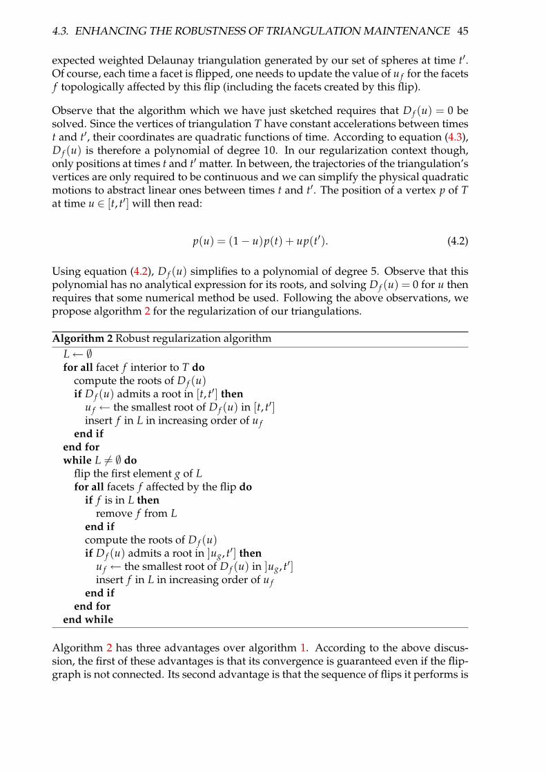
4.3. ENHANCING THE ROBUSTNESS OF TRIANGULATION MAINTENANCE 45
expected weighted Delaunay triangulation generated by our set of spheres at time t′.Of course, each time a facet is flipped, one needs to update the value of u f for the facetsf topologically affected by this flip (including the facets created by this flip).
Observe that the algorithm which we have just sketched requires that D f (u) = 0 besolved. Since the vertices of triangulation T have constant accelerations between timest and t′, their coordinates are quadratic functions of time. According to equation (4.3),D f (u) is therefore a polynomial of degree 10. In our regularization context though,only positions at times t and t′ matter. In between, the trajectories of the triangulation’svertices are only required to be continuous and we can simplify the physical quadraticmotions to abstract linear ones between times t and t′. The position of a vertex p of Tat time u ∈ [t, t′] will then read:
p(u) = (1− u)p(t) + up(t′). (4.2)
Using equation (4.2), D f (u) simplifies to a polynomial of degree 5. Observe that thispolynomial has no analytical expression for its roots, and solving D f (u) = 0 for u thenrequires that some numerical method be used. Following the above observations, wepropose algorithm 2 for the regularization of our triangulations.
Algorithm 2 Robust regularization algorithmL← ∅for all facet f interior to T do
compute the roots of D f (u)if D f (u) admits a root in [t, t′] then
u f ← the smallest root of D f (u) in [t, t′]insert f in L in increasing order of u f
end ifend forwhile L 6= ∅ do
flip the first element g of Lfor all facets f affected by the flip do
if f is in L thenremove f from L
end ifcompute the roots of D f (u)if D f (u) admits a root in ]ug, t′] then
u f ← the smallest root of D f (u) in ]ug, t′]insert f in L in increasing order of u f
end ifend for
end while
Algorithm 2 has three advantages over algorithm 1. According to the above discus-sion, the first of these advantages is that its convergence is guaranteed even if the flip-graph is not connected. Its second advantage is that the sequence of flips it performs is

46 CHAPTER 4. SOME IMPLEMENTATION DETAILS
uniquely determined, which was not the case for algorithm 1. The third advantage ofalgorithm 2 over algorithm 1 is that it handles the case of degenerated triangulations,which is the reason why we designed it.
We now propose an alternate robust regularization algorithm. Again, let f (u) be aninterior facet of T(u), a(u), b(u), c(u) its vertices and d(u) one of the vertices of T(u)so that conv( f (u) ∪ {d(u)}) is a maximal face of T(u). Call α(u) the vector product(b(u)− a(u)) ∧ (c(u)− a(u)). When the spheres move with time, conv( f ∪ {d}) maybecome flat. The time when simplex conv( f ∪ {d}) becomes flat is the smallest zero in[t, t′] of the following expression taken as a function of u:
H f (u) = [(c(u)− a(u)) ∧ (b(u)− a(u))] . [d(u)− a(u)] . (4.3)
using linear motions for the spheres according to equation (4.2), H f (u) is a polynomialof degree 3. Before any interior facet of T(u) becomes flat, T(u) is a triangulation thatcan be successfully regularized by algorithm 1. Following this observation, we proposealgorithm 3 as an alternative to algorithm 2.
The integer k used as a parameter of this algorithm must be strictly positive. It reflectsthe number of local degeneracies of T algorithm 1 is able to bear. Taking k = 1 meansthat the regularizations carried out in algorithm 3 will only process triangulations. Asa consequence, this algorithm prevents the failures of algorithm 1 caused by degenera-cies of the triangulation. The other parameter of algorithm 3 is the real number ε thatshould be strictly positive, yet small enough for the regularization to happen aroundthe expected value of u.
While algorithm 3 solves the degeneracy problems that caused algorithm 1 to fail, itstill relies on it for the regularization of a number of triangulations. Therefore, itstheoretical convergence is not guaranteed since it depends on the connectivity of theflip-graph. Again, since this theoretical failure never occurred in practical cases, thisdoes not seem to be much of a threat. Observe though that algorithm 3 has the advan-tage over algorithm 2 that analytical expressions exist for the roots of H f (u) since theyare polynomials of degree 3.
4.4 Experimental complexity analysis
As already mentioned in chapter 3, the complexity of our triangulation-based contactdetection method is proportional to the number of edges of the involved triangula-tions. There exist weighted Delaunay triangulations in three dimensions whose num-ber of edges are quadratic functions of their number of vertices. Following this, thetheoretical upper bound for the complexity of our contact detection method is O(n2).Since the computational cost of managing the triangulation is high, this suggests thatour contact detection algorithm is slower than the naive quadratic algorithm ! How-ever, the examples of quadratic Delaunay triangulations involve degenerate situationswhere most vertices lie on few line segments. Intuition suggests that the probability
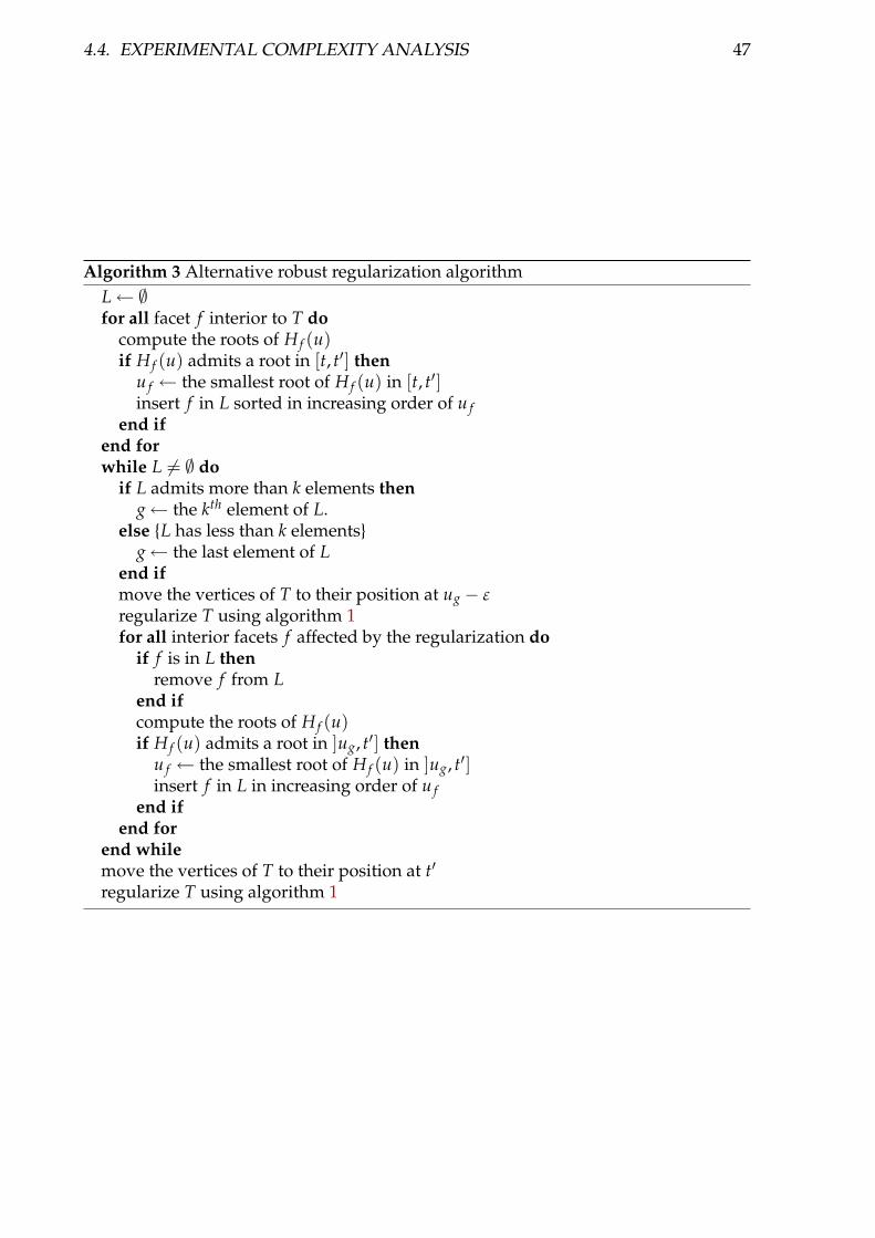
4.4. EXPERIMENTAL COMPLEXITY ANALYSIS 47
Algorithm 3 Alternative robust regularization algorithmL← ∅for all facet f interior to T do
compute the roots of H f (u)if H f (u) admits a root in [t, t′] then
u f ← the smallest root of H f (u) in [t, t′]insert f in L sorted in increasing order of u f
end ifend forwhile L 6= ∅ do
if L admits more than k elements theng← the kth element of L.
else {L has less than k elements}g← the last element of L
end ifmove the vertices of T to their position at ug −ε
regularize T using algorithm 1for all interior facets f affected by the regularization do
if f is in L thenremove f from L
end ifcompute the roots of H f (u)if H f (u) admits a root in ]ug, t′] then
u f ← the smallest root of H f (u) in ]ug, t′]insert f in L in increasing order of u f
end ifend for
end whilemove the vertices of T to their position at t′
regularize T using algorithm 1

48 CHAPTER 4. SOME IMPLEMENTATION DETAILS
of such events is small, and the bet of J.-A. Ferrez was that in all practical cases thenumber of edges of the triangulation is a linear number of its vertices. In this sectionwe present results on the overall complexity of the simulation process, obtained from aset of simulations and corresponding measures of the number of edges of the weightedDelaunay triangulation.
Figure 4.3: Snapshots of final states of numerical experiments. Left : experiment 1,right : experiment 3.
Snapshots of simulations performed with the non-spherical version of our code areshown in figure 4.3. Those experiments consist in pouring particles into a cylindricalcontainer of diameter 20 mm. This means that the number of particles gradually in-creases while the simulation proceeds. All particles have eight times the volume of asphere of diameter 1 mm, independently of their shape. Experiment 1 involves 250spherosimplices of each kind. Experiment 2 involves 500 spheres and 500 spherotetra-hedra, and experiments 3 and 4, 1000 spherocylinders each.
For the first two experiments, each particle only uses only one covering sphere for con-tact detection. This is achieved by calibrating every shape the same way the spherote-trahedra have been calibrated at the end of chapter 3. This constraint actually limits theparticle’s sharpness. Still, those particles are far from spherical and this way, the com-plexity of contact detection is the same as if all particles were spheres. In experiment3, spherocylinders have an elongation coefficient l/r of 3, where l is half the lengthof the segment constituting their skeletons and r is their radius. With such elongatedshapes, 5 covering spheres per particle are needed. In experiment 4, the elongation co-efficient l/r is 6, and 9 covering spheres are needed for a particle. In every experiment,ξm = 5× 10⁻⁵ m.
The computing time of the DEM process, including contact detection, is plotted infigure 4.4 against the number of simulated particles. In all cases it is almost linear.Observe that the slope of this linearity increases with particle elongation, naturally re-flecting that the number of possible contacts is higher for elongated particles. The inset

4.5. SOME INERTIA MATRICES 49
shows the number of edges of the triangulation, plotted against the number of cover-ing spheres and the four cases turn out to be identically linear. The slope of around 7 isclose to the coordination number of random close-packed spheres, indicating that ourmethod appropriately identifies the pairs of particles to be tested for contact.
0 200 6000
0.2
0.6
number of particles
time
inde
x
Exp. 1 and 2 Exp. 3Exp. 4
0 9000
70000
σ
ε
1000
1.0
0.4
0.8
400 800
0
Figure 4.4: Actual computing time of the DEM process plotted against the number ofsimulated particles for all four experiments. The time index is normalized to 1 for 1000of the last experiment’s spherosegments. Each point is averaged over 400 DEM itera-tions. Inset : number ε of edges in the triangulation versus the number σ of coveringspheres for the same experiments.
4.5 Some inertia matrices
Let P be a homogeneous particle, G its mass center and ω its spin vector. If P is sub-mitted to a total force f and a total momentum MG( f ) at point G, the motion equationsread:
{mG = fIGω = MG( f ) . (4.4)
where m is the mass of the particle and IG its inertia matrix at point G. One sees that IGis required when integrating the motion equations. Let (G, x, y, z) be an orthonormalreferential centered at point G. In this referential, the inertia moments of P read:
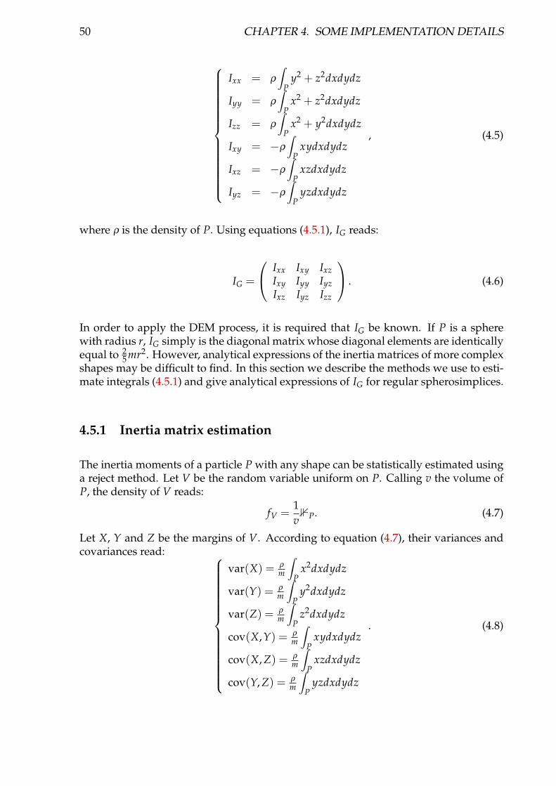
50 CHAPTER 4. SOME IMPLEMENTATION DETAILS
Ixx = ρ
∫P
y2 + z2dxdydz
Iyy = ρ
∫P
x2 + z2dxdydz
Izz = ρ
∫P
x2 + y2dxdydz
Ixy = −ρ
∫P
xydxdydz
Ixz = −ρ
∫P
xzdxdydz
Iyz = −ρ
∫P
yzdxdydz
, (4.5)
where ρ is the density of P. Using equations (4.5.1), IG reads:
IG =
Ixx Ixy IxzIxy Iyy IyzIxz Iyz Izz
. (4.6)
In order to apply the DEM process, it is required that IG be known. If P is a spherewith radius r, IG simply is the diagonal matrix whose diagonal elements are identicallyequal to 2
5 mr2. However, analytical expressions of the inertia matrices of more complexshapes may be difficult to find. In this section we describe the methods we use to esti-mate integrals (4.5.1) and give analytical expressions of IG for regular spherosimplices.
4.5.1 Inertia matrix estimation
The inertia moments of a particle P with any shape can be statistically estimated usinga reject method. Let V be the random variable uniform on P. Calling v the volume ofP, the density of V reads:
fV =1v1P. (4.7)
Let X, Y and Z be the margins of V. According to equation (4.7), their variances andcovariances read:
var(X) = ρm
∫P
x2dxdydz
var(Y) = ρm
∫P
y2dxdydz
var(Z) = ρm
∫P
z2dxdydz
cov(X,Y) = ρm
∫P
xydxdydz
cov(X, Z) = ρm
∫P
xzdxdydz
cov(Y, Z) = ρm
∫P
yzdxdydz
. (4.8)

4.5. SOME INERTIA MATRICES 51
Comparing the inertia moments and products of P with those variances and covari-ances we obtain the following expression for the inertia matrix:
IG = m
var(Y) + var(Z) −cov(X,Y) −cov(X,Y)−cov(X,Y) var(X) + var(Z) −cov(Y, Z)−cov(X, Z) −cov(Y, Z) var(X) + var(Y)
. (4.9)
A convenient way to estimate IG is therefore to estimate the variances and covariancesof the margins of V. This can be done by using an accept-reject method to simulate Vand by building the covariance matrix of the obtained data.
This method is convenient since it allows to compute the inertia matrix of any kindof shapes. The following subsection gives exact expressions of this matrix for sphero-cylinders and regular spherotetrahedra.
4.5.2 Exact inertia matrices of some spherosimplices
Let P be a spherocylinder with mass center G in the referential (G, x, y, z) as that shownin figure 4.5.
l
σ
x
G
y
z
r
Figure 4.5: A spherocylinder of radius r and skeleton σ of length l in the referential(G, x, y, z).
The integrals (4.5.1) then express as follow:Ixx = Iyy =
13πρr3l2 +
112
πρr2l3 +34πρr4l +
815
πρr5
Izz =12πρr4l +
815
πρr5
Ixy = Ixz = Iyz = 0
. (4.10)
Now assume that P is a regular spherotetrahedron with mass center G and radius r.
Calling A, B, C and D the vertices of P’s skeleton, and l the distance between G andany of those vertices. Let (G, x, y, z) be the referential shown in figure 4.5 in which the

52 CHAPTER 4. SOME IMPLEMENTATION DETAILS
A
B
C
D
G
x
y
z
l/3
l
A
B
C
x
yz
DG
Figure 4.6: The skeleton of a regular spherotetrahedron of mass center G and its asso-ciated referential (G, x, y, z). Right : view from above.
coordinates of A, B, C and D are:
A = (−√
23
l,−√
23
l,−13
l)
B = (2√
23
l, 0,−13
l)
C = (−√
23
l,
√23
l,−13
l)
D = (0, 0, l)
. (4.11)
The spherotetrahedron P is composed of the tetrahedron ABCD (figure 4.6), four prismswith thickness r and triangles ABC, ABD, ACD and BCD as bases, six portions of acylinder of radius r corresponding to the edges of ABCD and four portions of a sphereof radius r corresponding to the vertices of ABCD. The last three basic shapes areshown on figure 4.7 with the referentials we use to represent them.
E
F
HM
x
y
z
rF'
H'
E'
J
L
K
y
z
r
α
xN
L'
K'J'
r
αα
O
xy
αz
P
QR
E,E'
F,F'
H,H'
x
yz
M
J
LK
yzN
x
J'
L'K'
x
y
zO
P
Q
R
Figure 4.7: The three basic shapes that constitute a spherotetrahedron in addition toits skeleton. The referentials used to represent them are shown as well. Bottom : viewfrom above.
In order to find IG, we first calculate integrals (4.5.1) for each of the four basic shapes.By using Huygens theorem to translate the inertia moments and products, and rotating
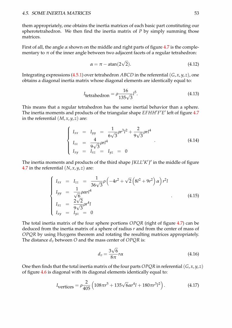
4.5. SOME INERTIA MATRICES 53
them appropriately, one obtains the inertia matrices of each basic part constituting ourspherotetrahedron. We then find the inertia matrix of P by simply summing thosematrices.
First of all, the angle α shown on the middle and right parts of figure 4.7 is the comple-mentary to π of the inner angle between two adjacent facets of a regular tetrahedron:
α = π − atan(2√
2). (4.12)
Integrating expressions (4.5.1) over tetrahedron ABCD in the referential (G, x, y, z), oneobtains a diagonal inertia matrix whose diagonal elements are identically equal to:
Itetrahedron = ρ16
135√
3l5. (4.13)
This means that a regular tetrahedron has the same inertial behavior than a sphere.The inertia moments and products of the triangular shape EFHH′F′E′ left of figure 4.7in the referential (M, x, y, z) are:
Ixx = Iyy =1
6√
3ρr3l2 +
29√
3ρrl4
Izz =4
9√
3ρrl4
Ixy = Ixz = Iyz = 0
. (4.14)
The inertia moments and products of the third shape JKLL′K′ J′ in the middle of figure4.7 in the referential (N, x, y, z) are:
Ixx = Izz =1
36√
3ρ
(−4r2 +
√2(
8l2 + 9r2)α
)r2l
Iyy =1√6ραrl4
Ixz =2√
29√
3ρr4l
Ixy = Iyz = 0
. (4.15)
The total inertia matrix of the four sphere portions OPQR (right of figure 4.7) can bededuced from the inertia matrix of a sphere of radius r and from the center of mass ofOPQR by using Huygens theorem and rotating the resulting matrices appropriately.The distance dv between O and the mass center of OPQR is:
dv =3√
68π
rα (4.16)
One then finds that the total inertia matrix of the four parts OPQR in referential (G, x, y, z)of figure 4.6 is diagonal with its diagonal elements identically equal to:
Ivertices = ρ2
405
(108πr5 + 135
√6αr4l + 180πr3l2
). (4.17)

54 CHAPTER 4. SOME IMPLEMENTATION DETAILS
The total inertia matrix of the four cylinder portions JKLL′K′ J′ (middle of figure 4.7)can be deduced from equations (4.15) and from the center of mass of JKLL′K′ J′ by us-ing Huygens theorem and rotating the resulting matrices appropriately. The distancede between N and the mass center of JKLL′K′ J′ reads:
de =4√
2r3√
3α(4.18)
The total inertia matrix of the six parts JKLL′K′ J′ in referential (G, x, y, z) of figure 4.6is diagonal with its diagonal elements identically equal to:
Iedges = ρ2
9√
3
(32rl +
√2(
9r2 + 10l2)α
)r2l. (4.19)
The total inertia matrix of the four triangular portions EFHH′F′E′ (left of figure 4.7) canbe deduced from equations (4.14) by using Huygens theorem and rotating the resultingmatrices appropriately. This total inertia matrix, expressed in the referential (G, x, y, z)of figure 4.6 is diagonal with its diagonal elements identically equal to:
Itriangles = ρ16
9√
3
(r2 + rl + l2
)rl2. (4.20)
According to expressions (4.13), (4.20), (4.19), (4.17), IG is diagonal with its diagonalelements identically equal to:
IP = 43ρ
(25πr5 +
√6αr4l + 2
3
(π + 10√
3
)r3l2 + 1
3√
3
(4 + 5
√2α
)r2l3 + 4
3√
3rl4 + 4
45√
3l5
).
(4.21)This means that the inertia matrix of P is that of a sphere.

Part II
Applications


Chapter 5
A Study of Arching Effects andFlowability
Confined granular flows are known to arch suddenly about their confining bounar-ies under certain circumstances. As an effect, this causes jamming, i.e. prevents anyfurther flowing motion of the medium. While this phenomenon may be due to mi-croscopic interactions in fine powders, it also occurs with large grains in the form ofmechanical equilibria induced by macroscopic forces. This phenomenon, refered toas “arching effect” is still little understood. It is a limiting cause for the flowability ofpowders, i.e. their ability to flow.
While the arching effect itself is difficult to encompass as a complex collective be-haviour, flowability is a simple property that can be measured in a variety of waysand may provide insights into the mechanisms underlying the formation of arches.We choose here to investigate the flowability experiment that consists in opening ahole at the bottom of a grain-filled container and to check whether or not the mediumflows.
The probability for such an assembly of beads of given granulometry and surface prop-erties to flow in this experiment will be estimated as a function of the opening hole’sdiameter D. This will allow to determine the opening hole’s diameter for which theprobability for this medium to flow is 0.5, which we call its mean critical diameter Dc.This diameter is the quantity we use to characterize the flowability of an assembly ofbeads.
Surface properties of the involved beads will be characterized with their mutual stat-ical friction coefficient µ. Numerical trials have been conducted with monodispersebead assemblies and several friction coefficients. Experiments performed on the samemonodisperse assemblies composed of steel beads show that those numerical modelsprovide realistic values for Dc.
Finally, measures of Dc for bidisperse assemblies of beads are obtained from numeri-cally simulated trials of our flowability experiment. Those results show that for a given

58 CHAPTER 5. A STUDY OF ARCHING EFFECTS AND FLOWABILITY
friction coefficient, Dc only depends on the bead’s mass-average diameter, which sug-gests that a law be formulated about the flowability of polydisperse bead assemblies.
5.1 The flowability experiment
In order to measure the flowability of a powder, we proceed with the following exper-iment. The setup used is a plexiglas cylinder with interchangeable aluminum discs atthe bottom that feature circular holes in their centers. The inner diameter of the cylin-der is 5 cm and the bottom discs have various diameters D for their central holes. Thehole of the bottom disc can be obturated using a shutter in aluminum as shown on theleft side of figure 5.1.
pierceddisc
shutter
plexiglas cylinder
D D
5 cm 5 cm
Figure 5.1: The experimental setup we use to measure the flowability of a bead as-sembly (left) and its numerical model (right). The shutter and the pierced disc of theexperimental setup are numerically modeled by a circular hole sketched as a dottedline that can either be opened or closed.
The experiment proceeds as follows : the beads are poured into the cylinder while thehole of the bottom disc is obturated by the shutter. The granular piling to be processedis then obtained when a mechanical equilibrium is reached, all the beads being at rest.Finally the shutter is suddenly pulled out and the medium either flows through thehole of the bottom disc or blocks which is the result of the experiment. For our experi-mental trials, we used steel beads of diameters 1.0 mm, 4.0 mm, 5.0 mm and 7.0 mm.All trials were carried out with as close as possible to 0.575 kg of those steel beads, re-sulting in a filling height of around 6.5 cm independently of the bead diameters. Whenprocessing fine powders, a funnel is used to pour the medium into the cylinder. In ourcase of large beads however, this is superfluous. Indeed, using a funnel with a largeenough opening for our beads to flow freely through it actually amounts to use nofunnel at all.
Our flowability experiment were numerically reproduced with the Distinct ElementsMethod. Contacts will be modeled with a contact time of tc = 6.10−4 s and a restitu-
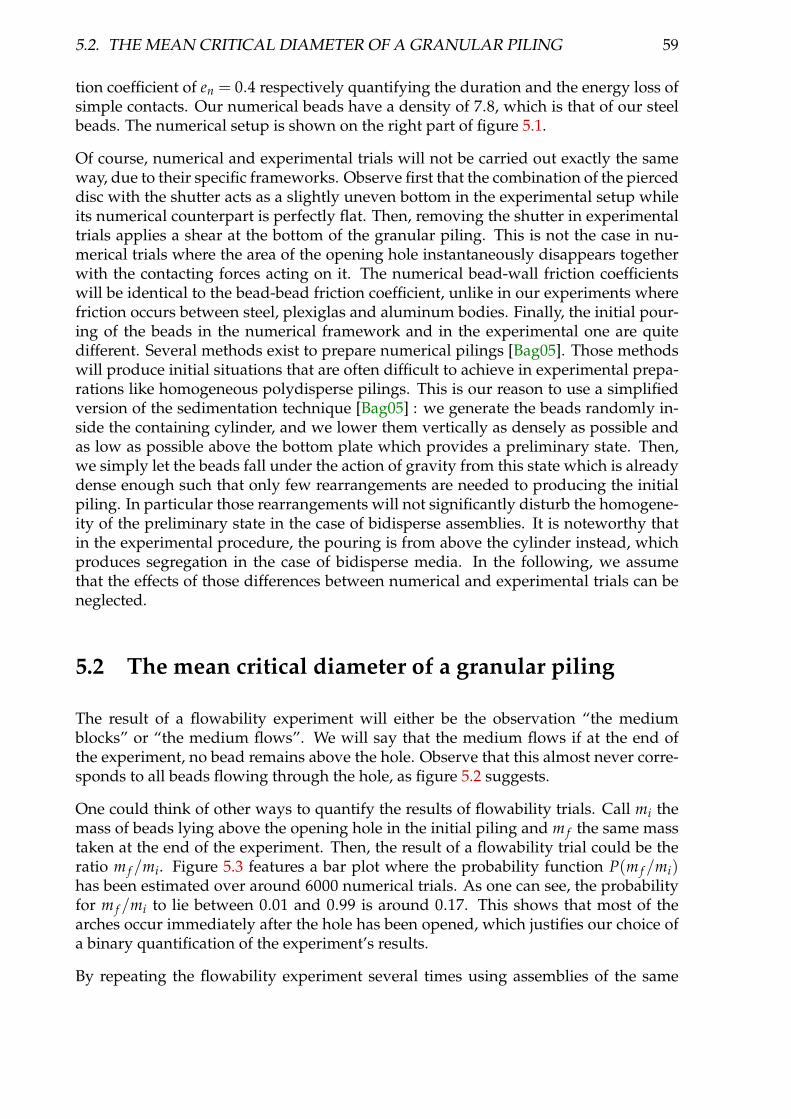
5.2. THE MEAN CRITICAL DIAMETER OF A GRANULAR PILING 59
tion coefficient of en = 0.4 respectively quantifying the duration and the energy loss ofsimple contacts. Our numerical beads have a density of 7.8, which is that of our steelbeads. The numerical setup is shown on the right part of figure 5.1.
Of course, numerical and experimental trials will not be carried out exactly the sameway, due to their specific frameworks. Observe first that the combination of the pierceddisc with the shutter acts as a slightly uneven bottom in the experimental setup whileits numerical counterpart is perfectly flat. Then, removing the shutter in experimentaltrials applies a shear at the bottom of the granular piling. This is not the case in nu-merical trials where the area of the opening hole instantaneously disappears togetherwith the contacting forces acting on it. The numerical bead-wall friction coefficientswill be identical to the bead-bead friction coefficient, unlike in our experiments wherefriction occurs between steel, plexiglas and aluminum bodies. Finally, the initial pour-ing of the beads in the numerical framework and in the experimental one are quitedifferent. Several methods exist to prepare numerical pilings [Bag05]. Those methodswill produce initial situations that are often difficult to achieve in experimental prepa-rations like homogeneous polydisperse pilings. This is our reason to use a simplifiedversion of the sedimentation technique [Bag05] : we generate the beads randomly in-side the containing cylinder, and we lower them vertically as densely as possible andas low as possible above the bottom plate which provides a preliminary state. Then,we simply let the beads fall under the action of gravity from this state which is alreadydense enough such that only few rearrangements are needed to producing the initialpiling. In particular those rearrangements will not significantly disturb the homogene-ity of the preliminary state in the case of bidisperse assemblies. It is noteworthy thatin the experimental procedure, the pouring is from above the cylinder instead, whichproduces segregation in the case of bidisperse media. In the following, we assumethat the effects of those differences between numerical and experimental trials can beneglected.
5.2 The mean critical diameter of a granular piling
The result of a flowability experiment will either be the observation “the mediumblocks” or “the medium flows”. We will say that the medium flows if at the end ofthe experiment, no bead remains above the hole. Observe that this almost never corre-sponds to all beads flowing through the hole, as figure 5.2 suggests.
One could think of other ways to quantify the results of flowability trials. Call mi themass of beads lying above the opening hole in the initial piling and m f the same masstaken at the end of the experiment. Then, the result of a flowability trial could be theratio m f /mi. Figure 5.3 features a bar plot where the probability function P(m f /mi)has been estimated over around 6000 numerical trials. As one can see, the probabilityfor m f /mi to lie between 0.01 and 0.99 is around 0.17. This shows that most of thearches occur immediately after the hole has been opened, which justifies our choice ofa binary quantification of the experiment’s results.
By repeating the flowability experiment several times using assemblies of the same

60 CHAPTER 5. A STUDY OF ARCHING EFFECTS AND FLOWABILITY
Figure 5.2: Top view of the final situations for four flowability experiments where themedium flowed. A photo of a real-world experiment is shown bottom-right while thethree others are snapshots of the simulated setup.
0.0 0.02 0.04 0.96 0.98 1.0
0.1
0.2
0.3
0.4
0.5
m /m
P( )
f i
m /mf i
Figure 5.3: The probability function P(m f /mi) of the ratio of the masses lying abovethe opening hole after (m f ) and before (mi) the hole has been opened, estimated over6246 monodisperse numerical trials.
beads, one can estimate the probability for them to flow through a hole of given di-ameter D. This allows in particular to find the statistical diameter Dc of the openinghole for which the probability for a medium to flow is 0.5. This diameter, called meancritical diameter is the quantity we choose to characterize the flowability of bead assem-blies. In order to estimate Dc, we process the flowability results using a generalizedlinear model [DH97]. An example of estimation this statistical model provides for Dcis shown on figure 5.4. All the confidence intervals we provide for Dc were found by

5.2. THE MEAN CRITICAL DIAMETER OF A GRANULAR PILING 61
applying a bootstrap method [DH97] on the flowability results.
19.0 22.0 25.00.0
0.5
1.0
Opening diameter (mm)
Pro
por
tion
of flow
ing t
ries
D c = 22.0716 mm
Figure 5.4: The proportion of flowing trials as a function of the diameter of the openinghole obtained from 510 numerical trials with monodisperse assemblies of beads ofdiameter 6 mm and mutual friction coefficient of µ = 0.8. The raw results are indicatedas small circles of coordinates (D, r) where D is the opening diameter and r is 1 whenthe medium flows and 0 instead. The dots show the proportion of flowing trials inwindows 0.4 mm large. The solid line shows the fit of the raw data obtained with anappropriate generalized linear model.
Intuition suggests that for a large enough number of flowability trials, the proportionof flowing trials will be an increasing function of the diameter of the opening hole.While it seems relevant to assume it, this property still needs to be checked. Indeed,we made at most 990 trials per medium with same granulometry and mutual frictioncoefficient. If ever this property turns out to be false, our mean critical diameter wouldbe of a purely statistical nature but still could be defined as the diameter Dc for whichthe probability for the opening diameter of a flowing trial to be inferior to Dc is 0.5.Thus, our statistical measure keeps its intrinsic physical meaning.
Now consider some granular piling obtained prior to the hole opening. Our numericalframework makes it possible to try several diameters for the hole opening under thisparticular piling. One may wonder if a critical diameter exists for the hole, above whichthis piling will flow and below which an arch will form. Observe that this question can-not be answered by performing trials in our experimental framework. A same piling,prepared with beads of diameter 6 mm and mutual friction coefficient of µ = 0.8, wassubject to a set of 5000 flowability experiments with different diameters. The resultsof those trials, depicted in figure 5.5 clearly show that the answer to the above ques-tion is no. There are values D− and D+ so that arching always occurs for D < D− andnever for D > D+, but the interval [D−, D+] is significantly wide. This phenomenoncould be further investigated, for example by finding how D+−D− depends on beads’diameters and mutual friction coefficients.

62 CHAPTER 5. A STUDY OF ARCHING EFFECTS AND FLOWABILITY
24.0 25.0 26.0 27.00.0
0.2
0.4
0.6
0.8
1.0
Opening diameter (mm)
Pro
por
tion
of flow
ing t
ries
Figure 5.5: The proportion of flowing trials in windows 0.1 mm large obtained bysubmitting a given monodisperse piling of beads to a series of 5000 flowability trieswith opening diameters ranging from 23.0 mm to 28.0 mm. The diameter of the beadsis 6 mm and their mutual friction coefficient is µ = 0.8.
5.3 The influence of friction
The flowability of a powder is known [Gio80] to reflect the friction coefficient of itsconstituting particles. In our macroscopic framework, this is still the case as shownin figure 5.6 for monodisperse sets of beads with diameters 4 mm, 5 mm and 7 mm.In particular, the mean critical diameter is a globally increasing function of the inter-particulate friction coefficient. Observe also that the influence of friction on the meancritical diameter is well marked for low values of the friction coefficient while it canpractically be neglected for high ones.
Φ (mm) Dc (mm)1.0 3.88± 0.154.0 14.92± 0.235.0 17.46± 0.377.0 21.85± 1.24
Table 5.1: Results of experimental trials on monodisperse sets of steel beads.
The mean critical diameters measured from our experiments with steel beads are shownin table 5.1 and reported on figure 5.6 for Φ = 4.0 mm, Φ = 5.0 mm and Φ = 7.0 mm.One can see that numerical and experimental trials show good agreement even thoughtheir respective frameworks are different. Observe that the differences between exper-imental values of Dc are qualitatively identical to the differences between numericalcurves. This shows that the numerical model is coherent in the way it handles friction,and proves appropriate in the framework of flowability experiments.
Mean critical diameters were measured for monodisperse media with various beaddiameters and friction coefficients. All those monodisperse results are shown on figure
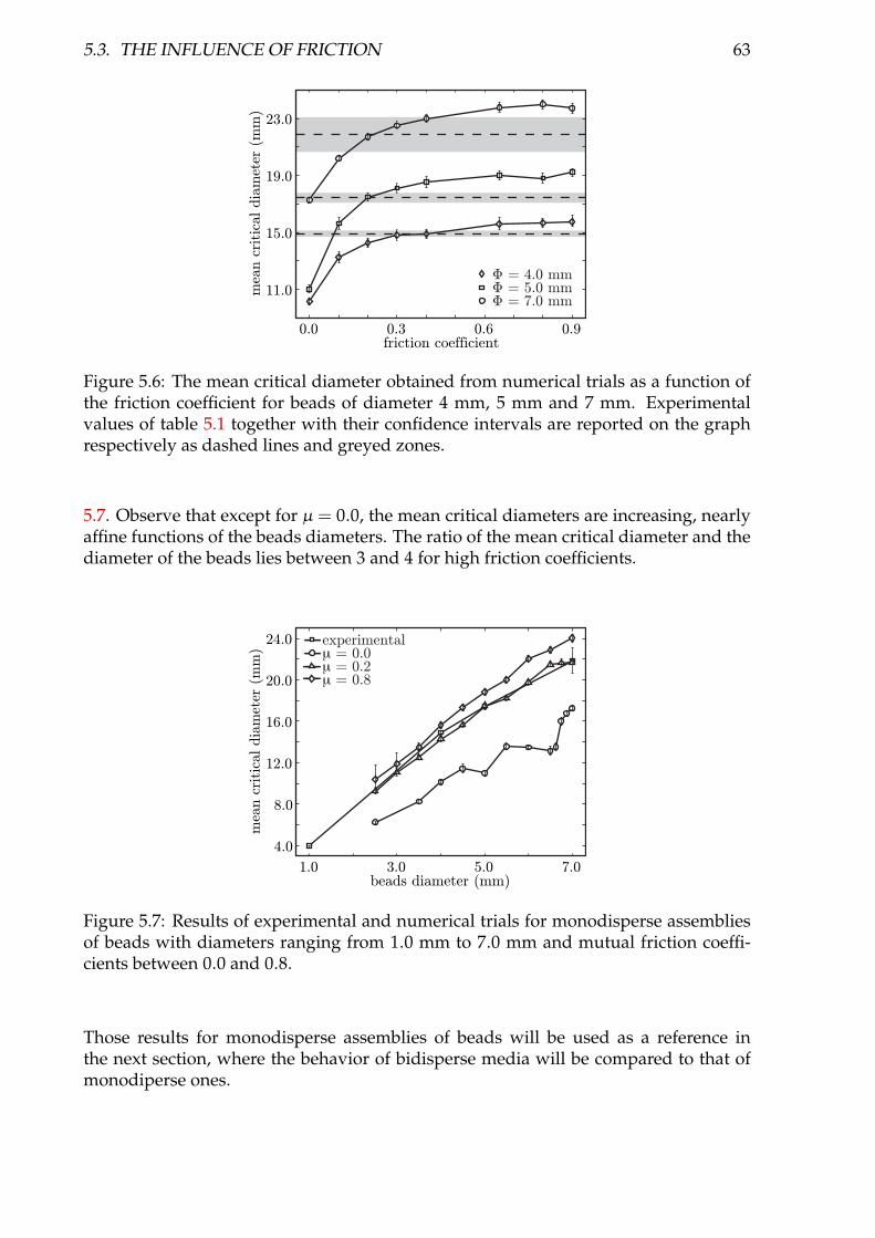
5.3. THE INFLUENCE OF FRICTION 63
0.0 0.3 0.6 0.9
11.0
15.0
19.0
23.0
friction coefficient
© = 7.0 mm© = 5.0 mm© = 4.0 mm
mea
n c
ritica
l dia
met
er (
mm
)
Figure 5.6: The mean critical diameter obtained from numerical trials as a function ofthe friction coefficient for beads of diameter 4 mm, 5 mm and 7 mm. Experimentalvalues of table 5.1 together with their confidence intervals are reported on the graphrespectively as dashed lines and greyed zones.
5.7. Observe that except for µ = 0.0, the mean critical diameters are increasing, nearlyaffine functions of the beads diameters. The ratio of the mean critical diameter and thediameter of the beads lies between 3 and 4 for high friction coefficients.
1.0 3.0 5.0 7.0
4.0
8.0
12.0
16.0
20.0
24.0
beads diameter (mm)
mea
n c
ritica
l dia
met
er (
mm
)
experimentalμ = 0.0μ = 0.2μ = 0.8
Figure 5.7: Results of experimental and numerical trials for monodisperse assembliesof beads with diameters ranging from 1.0 mm to 7.0 mm and mutual friction coeffi-cients between 0.0 and 0.8.
Those results for monodisperse assemblies of beads will be used as a reference inthe next section, where the behavior of bidisperse media will be compared to that ofmonodiperse ones.
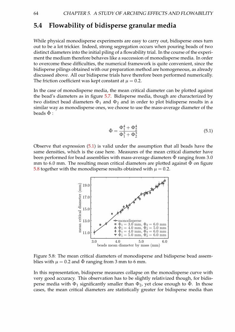
64 CHAPTER 5. A STUDY OF ARCHING EFFECTS AND FLOWABILITY
5.4 Flowability of bidisperse granular media
While physical monodisperse experiments are easy to carry out, bidisperse ones turnout to be a lot trickier. Indeed, strong segregation occurs when pouring beads of twodistinct diameters into the initial piling of a flowability trial. In the course of the experi-ment the medium therefore behaves like a succession of monodisperse media. In orderto overcome these difficulties, the numerical framework is quite convenient, since thebidisperse pilings obtained with our preparation method are homogeneous, as alreadydiscussed above. All our bidisperse trials have therefore been performed numerically.The friction coefficient was kept constant at µ = 0.2.
In the case of monodisperse media, the mean critical diameter can be plotted againstthe bead’s diameters as in figure 5.7. Bidisperse media, though are characterized bytwo distinct bead diameters Φ1 and Φ2 and in order to plot bidisperse results in asimilar way as monodisperse ones, we choose to use the mass-average diameter of thebeads Φ :
Φ =Φ4
1 + Φ42
Φ31 + Φ3
2(5.1)
Observe that expression (5.1) is valid under the assumption that all beads have thesame densities, which is the case here. Measures of the mean critical diameter havebeen performed for bead assemblies with mass-average diameters Φ ranging from 3.0mm to 6.0 mm. The resulting mean critical diameters are plotted against Φ on figure5.8 together with the monodisperse results obtained with µ = 0.2.
3.0 4.0 5.0 6.0
11.0
13.0
15.0
17.0
19.0
beads mean diameter by mass (mm)
monodisperse© = 3.0 mm, © = 6.0 mm1 2© = 4.0 mm, © = 5.0 mm1 2© = 4.0 mm, © = 6.0 mm1 2© = 5.0 mm, © = 6.0 mm1 2
mea
n c
ritica
l dia
met
er (
mm
)
Figure 5.8: The mean critical diameters of monodisperse and bidisperse bead assem-blies with µ = 0.2 and Φ ranging from 3 mm to 6 mm.
In this representation, bidisperse measures collapse on the monodisperse curve withvery good accuracy. This observation has to be slightly relativized though, for bidis-perse media with Φ1 significantly smaller than Φ2, yet close enough to Φ. In thosecases, the mean critical diameters are statistically greater for bidisperse media than

5.5. CONCLUSIONS 65
for monodisperse ones. This can be explained in terms of segregation. Indeed, suchgranular assemblies feature a small number of large beads that are significantly largerthan the others. This leads to a strong tendency to segregate. Large beads actuallymigrate to the top and remain there while small beads flow through the hole. Whenthe large beads finally reach the hole, most of the time they gather in an arch such asthose shown in figure 5.9.
Figure 5.9: Top view of two arches involving mostly big beads that segregated duringthe flow.
Apart from this, bidisperse and monodisperse results fit very well. Moreover, one mayobserve that two bidisperse media with same Φ but different diameters for their con-stituting beads will have the same mean critical diameter. Those observations leadus to formulate the following tentative law : for fixed interparticulate friction, mean crit-ical diameters of homogeneous bidisperse bead assemblies only depend on their mass-averagediameters.
For low friction coefficients, the dependence of flowability on the diameter of the beadsis more erratic than for high frictions (figure 5.7). A further question is the validity ofthe above law for such frictions, which would allow to decide whether it is intrinsic tobead assemblies or only a linear dependance between the set of involved bead diam-eters. Figure 5.10 reports results of either monodisperse and bidisperse tries obtainedwith µ = 0.0 and Φ ranging from 5.0 mm to 7.0 mm. Observe that the monodispersecurve is strongly increasing for Φ < 5.5 and Φ > 6.5 and approximately constant inbetween. One can see that bidisperse results collapse well on this highly non-linearcurve, which further validates our flowability law.
Observe that this law was checked for bidisperse and monodisperse bead sets withµ = 0.0 and µ = 0.2. Polydisperse media with wider ranges of diameters still have tobe investigated, though.
5.5 Conclusions
By performing both experimental and numerical trials, we have shown that distinctelement methods are appropriate to evaluate the flowability of monodisperse bead as-semblies. Once again, this suggests that those numerical models successfully capturethe behavior of statical granular media. It has also been observed that the dependence
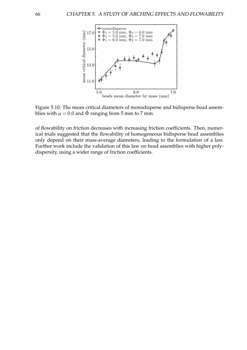
66 CHAPTER 5. A STUDY OF ARCHING EFFECTS AND FLOWABILITY
5.0 6.0 7.0
11.0
13.0
15.0
17.0
beads mean diameter by mass (mm)
mea
n c
ritica
l dia
met
er (
mm
)
monodisperse© = 5.0 mm, © = 6.0 mm1 2© = 5.0 mm, © = 7.0 mm1 2© = 6.0 mm, © = 7.0 mm1 2
Figure 5.10: The mean critical diameters of monodisperse and bidisperse bead assem-blies with µ = 0.0 and Φ ranging from 5 mm to 7 mm.
of flowability on friction decreases with increasing friction coefficients. Then, numer-ical trials suggested that the flowability of homogeneous bidisperse bead assembliesonly depend on their mass-average diameters, leading to the formulation of a law.Further work include the validation of this law on bead assemblies with higher poly-dispersity, using a wider range of friction coefficients.
Chapter 6
Spherocylinder Crystallization
For our first numerical experiments with non-spherical particles, we use spherocylin-ders, and shake them in a cylindrical container. As a result, we observe them crystallizevertically and faithfully reproduce the corresponding results of physical experimentsfrom the literature [VLMJ00].
We discuss the mechanisms underlying to this phenomenon that recalls of a crystallinegrowth germinating about the boundaries of the container. Note that while this crys-tallization is catalyzed by the boundaries in our setup, there actually are several causesfor this phenomenon. It has been suggested [BNK03; RPL05b] that the void-fillingprocess is another mechanism leading to spherocylinder crystallization. Moreover, ithas been shown [RPL05b] that vertical ordering also happens without the influence ofwalls.
6.1 The Experiments
We simulate the rearrangement of mono-disperse populations of spherocylinders en-closed within a cylindrical container subject to vertical tapping. In order to do this,we use a cylindrical container of base diameter D, which is sufficiently high so thatthe particles cannot escape from it. Its base is mobile and can be subject to a 30 Hzsinusoidal vertical oscillation whose amplitude a can be chosen, whereas its verticalwall remains motionless. The grains used for the rearrangement are spherocylindersof diameter δ and elongation parameter φ = λ/δ. Population size is Np. Simulationprocesses are initialized by randomly placing the particles within the cylinder, the di-rections of their shafts being uniformly distributed, and letting them settle under theaction of gravity. Once the kinetic energy has dropped to zero, we start the vibrations.
We monitor the intensity of the vibrations via the ratio Γ = a(2πν)2
g , that is the maximalacceleration brought by the bottom plane to the granular packing. Individual grainshave density ρ and we further define the medium’s volumetric density ρm as the ra-tio of the total volume occupied by the grains divided by the volume of the enclosing

68 CHAPTER 6. SPHEROCYLINDER CRYSTALLIZATION
truncated cylinder (upon elimination of outliers). In order to capture the reorderingbehavior as a function of the height of the enclosing cylinder, the latter is subdividedinto four horizontal layers of equal thickness h = 4 mm, numbered in increasing orderfrom bottom to top. In other words, layer i is lying between heights (i− 1).h and i.h.
We monitor the behavior of the medium in terms of the mean angle between the grainshafts and the bottom plane as well as its volumetric density ρm, both globally andlayer by layer. Experiments an3, ..., an9 were designed to investigate the way elongatedgrains rearrange, and in particular to observe possible re-orderings which would recalla phase transition. Among those seven experiments, the main one is an6. Experimentan9 involves shorter grains in order to show how the elongation parameter φ changesthe rearrangement behavior. In this experiment, the number of grains is chosen so thatthe initial filling height is closest possible to that of an6. The other five experimentswere carried out to investigate possible influence of the restitution coefficient en andthe vibration intensity Γ on the results.
The parameter values for the various simulations we carried out are given in table 6.1
∆t (s) tc (s) en Γ φ δ (m) D (m) Npan3 2× 10⁻⁵ 6× 10⁻⁴ 0.1 2.0 4.00 0.523× 10⁻³ 8× 10⁻³ 1000an4 2× 10⁻⁵ 6× 10⁻⁴ 0.2 2.0 4.00 0.523× 10⁻³ 8× 10⁻³ 1000an5 2× 10⁻⁵ 6× 10⁻⁴ 0.4 1.5 4.00 0.523× 10⁻³ 8× 10⁻³ 1000an6 2× 10⁻⁵ 6× 10⁻⁴ 0.4 2.0 4.00 0.523× 10⁻³ 8× 10⁻³ 1000an7 2× 10⁻⁵ 6× 10⁻⁴ 0.4 2.5 4.00 0.523× 10⁻³ 8× 10⁻³ 1000an8 2× 10⁻⁵ 6× 10⁻⁴ 0.8 2.0 4.00 0.523× 10⁻³ 8× 10⁻³ 1000an9 2× 10⁻⁵ 6× 10⁻⁴ 0.4 2.0 2.83 0.523× 10⁻³ 8× 10⁻³ 1414
Table 6.1: Experiments of vibrating mono-disperse media
6.2 Crystallization mechanisms
Lateral snapshots of experiment an6 at various evolution stages are given in figure 6.1.In a qualitative way, we see that the spherocylinders rearrange vertically to a highlyordered state, at least along the cylinder boundary. The cuts of the cylinder with aplane through its axis shown in figure 6.1 further show that this particular rearrange-ment also occurs in the middle of the container. Obviously the concurring shapes andsizes of both container and grains play a decisive role on crystallization processes. Inparticular, this is why the spherocylinders tend to crystallize vertically, achieving ahigh volumetric density. The final arrangements reported in [ATC03] for Metropolis-Monte-Carlo simulations of spherocylindric populations are not crystalline. For obvi-ous reasons one can not draw any conclusions about the dynamic behavior of real grainrearrangements from the Monte-Carlo process. Furthermore, the final density attainedin [ATC03] corresponds to a metastable state of significantly lower volumetric densitythan that of the crystallized medium. This does not come as a surprise since such ametastable state is very hard to escape, the crystallization process certainly having a
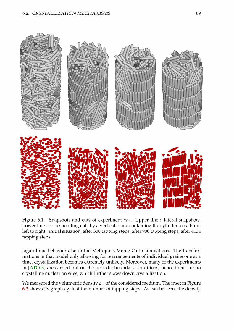
6.2. CRYSTALLIZATION MECHANISMS 69
Figure 6.1: Snapshots and cuts of experiment an6. Upper line : lateral snapshots.Lower line : corresponding cuts by a vertical plane containing the cylinder axis. Fromleft to right : initial situation, after 300 tapping steps, after 900 tapping steps, after 4134tapping steps
logarithmic behavior also in the Metropolis-Monte-Carlo simulations. The transfor-mations in that model only allowing for rearrangements of individual grains one at atime, crystallization becomes extremely unlikely. Moreover, many of the experimentsin [ATC03] are carried out on the periodic boundary conditions, hence there are nocrystalline nucleation sites, which further slows down crystallization.
We measured the volumetric density ρm of the considered medium. The inset in Figure6.3 shows its graph against the number of tapping steps. As can be seen, the density
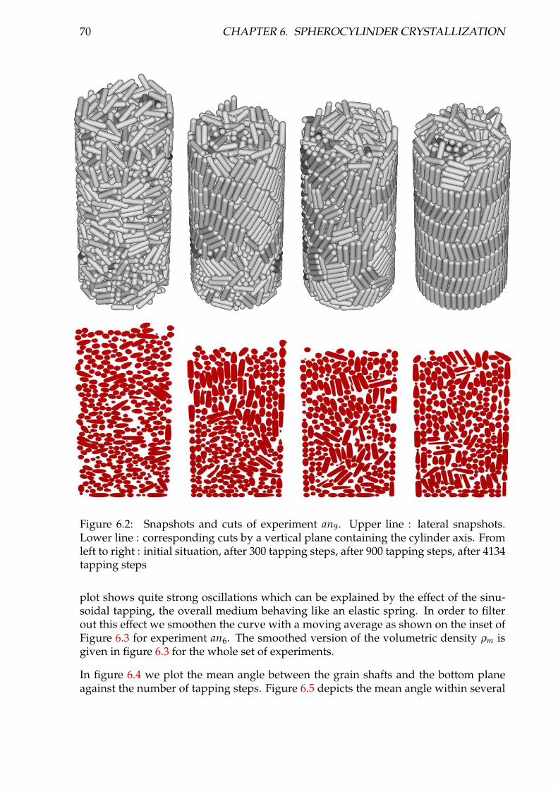
70 CHAPTER 6. SPHEROCYLINDER CRYSTALLIZATION
Figure 6.2: Snapshots and cuts of experiment an9. Upper line : lateral snapshots.Lower line : corresponding cuts by a vertical plane containing the cylinder axis. Fromleft to right : initial situation, after 300 tapping steps, after 900 tapping steps, after 4134tapping steps
plot shows quite strong oscillations which can be explained by the effect of the sinu-soidal tapping, the overall medium behaving like an elastic spring. In order to filterout this effect we smoothen the curve with a moving average as shown on the inset ofFigure 6.3 for experiment an6. The smoothed version of the volumetric density ρm isgiven in figure 6.3 for the whole set of experiments.
In figure 6.4 we plot the mean angle between the grain shafts and the bottom planeagainst the number of tapping steps. Figure 6.5 depicts the mean angle within several

6.2. CRYSTALLIZATION MECHANISMS 71
100
101
102
103
104
0.5
0.6
0.7
0.8
t+1
an3
an4
an5
an6
an7
an8
an9
ρm
Figure 6.3: Smoothed density ρm plotted versus the number of tapping steps t for ex-periments an3-an9. Inset : oscillations of the measured density and its moving averagesmoothed version for experiment an6
horizontal subdivisions of the container. The mean angle does not show the sameoscillatory behavior as the volumetric density. A possible explanation might be thatduring a tapping oscillation, the angle variations tend to average out. We see that thebeginning of a phase transition with respect to the angle takes place at approximatelyconstant density (between 10 and 100 tapings). Observe that the crystallization processas measured by the volumetric density starts after about 100 tapping steps, behavinglogarithmically from there on until it reaches a value of ρm = 0.75 for the highest afterabout 2000 tapings. This value is not very far from the maximum possible densityof tightly packed spherocylinders in an unbounded three-dimensional space, whichequals ρmax
m = π6
3φ+2√3φ+√
2, that is ρmax
m = 0.8787 when φ = 4.0.
Measured by the mean angle, the crystallization process starts after 10 tapings alreadyand behaves logarithmically until it saturates after approximately 1000 tapings for ex-periments an3, an5 and an9. Experiments an3 and an5 do not show a logarithmic behav-ior during the re-ordering process. The restitution coefficient used in experiment an3 ismuch lower than that used in the other experiments. This causes the energy reaching

72 CHAPTER 6. SPHEROCYLINDER CRYSTALLIZATION
100
101
102
103
104
0
10
20
30
40
50
60
70
80
90
t+1
Mea
n A
ngle
(de
gree
s)an
3an
4an
5an
6an
7an
8an
9
Figure 6.4: Mean angle between the particles shafts and the bottom plane versus thenumber t of tapping steps for several experiments
the grains to be small, which limits their motion. However, we see no dependence onen for en ≥ 0.2 (experiments an4, an6, an8). This would mean that in experiment an3the energy available to the system is too small for it to reach the dynamical regimefound in experiments an4, an6 and an8. For experiment an5, the value of Γ is prettylow, which means that little energy is brought to the system. In this case also, the otherexperiments (an6, an7) show there is no dependence on Γ for Γ ≥ 2.0. Again, this sug-gests that the energy available to the system is not sufficient to reach the dynamics ofexperiments an4, an6 and an8. While experiment an9 exhibits the same logarithmic re-ordering as experiments an4, an6, an7 and an8, figure 6.4 shows that this logarithmicpart is shorter and that the saturation takes place at a lower value of the mean angle.This shows that while the dynamics of the re-ordering seems not to be dependent ofthe elongation parameter, the saturation process is. It might be that with small valuesof Φ, the grains have more freedom to arrange in a disordered state, and the transitionto a crystalline ordering is less probable.
Another possibility is that the cylinder shape has less influence on short grains thanon long ones. Indeed when a slanted particle touches a cylindrical wall at two points,
6.2. CRYSTALLIZATION MECHANISMS 73
a torque develops that tends to erect it. The magnitude of this torque increases withparticle lenght. It can be observed that the logarithmic stage of reordering is mainlydue to global rearrangement processes (convection), whereas the saturation stage isruled by local rearrangements. The logarithmic rearrangement behavior correspondsto that observed for media composed of identical spherical grains.
Figure 6.5 shows that excepting top and bottom layers, the mean angle increases mono-tonically to eventually stay between 80 and 90 degrees for experiments an3, an4, an6,an8 and between 60 and 80 degrees for experiments an5, an7, and an9. This meansthat the crystallization does not only occur along the container wall but involves allgrains in those layers. Figure 6.5 also shows that in the logarithmic re-ordering stage,layers seem to reorder from the top to the bottom as the mean angle in a layer is al-ways lower than that of the higher layers. In the saturation stage, this behavior invertsfor the two central layers while the mean angle still increases in the lowest layer anddrops in the topmost layer as it gradually empties. Again, this suggests that the natureof rearrangement processes in the logarithmic and saturation phases is not the same,the former being essentially due to global phenomena and the latter involving localrearrangements in a mostly static medium. This behavior matches that observed in[VLMJ00] on experiments with real elongated grains. Quantitatively, the dynamics ofour simulated media fits well that reported there. In particular, the time slots for bothreordering processes match. The reordering is logarithmic in both cases, and the initialand final volumetric densities also agree.
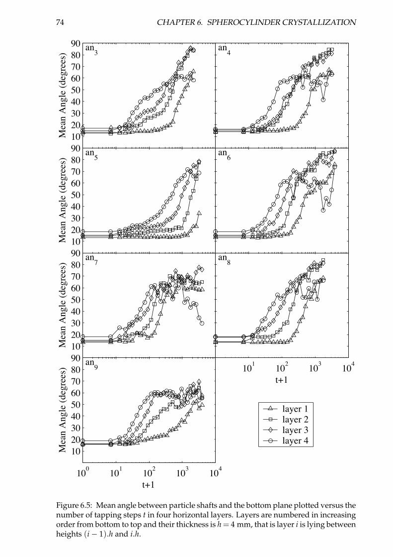
74 CHAPTER 6. SPHEROCYLINDER CRYSTALLIZATION
10
20
30
40
50
60
70
80
90
Mean
An
gle
(d
eg
rees)
an3
an4
10
20
30
40
50
60
70
80
90
Mean
An
gle
(degre
es)
an5
an6
10
20
30
40
50
60
70
80
90
Mean A
ngle
(deg
rees)
an7
101
102
103
104
an8
100
101
102
103
104
10
20
30
40
50
60
70
80
90
Mean
Ang
le (
deg
rees)
an9
t+1
t+1
5 layer 1
layer 2
layer 3
layer 4
Figure 6.5: Mean angle between particle shafts and the bottom plane plotted versus thenumber of tapping steps t in four horizontal layers. Layers are numbered in increasingorder from bottom to top and their thickness is h = 4 mm, that is layer i is lying betweenheights (i− 1).h and i.h.
Chapter 7
On the segregation of spheres andtetrahedra
Granular media can behave like solids, liquids and also gas depending on the con-ditions they are submitted to. Some of their behaviors though, cannot be classifiedin any of these three states of matter. Granular segregation, also known as Brazil nuteffect belongs to this range of behavior that escapes usual classifications. The Brazilnut effect is observed in particular when particles of different sizes are shaken. Par-ticles with same sizes will gather, producing size inhomogeneities that contradict theintuition whereby diffusion should occur. It was first observed that large particleswould migrate upwards under vibrations [MLNJ01; KJN93; DRC93; RSPS87]. Particledensity was found to play a role too, though less important than particle size in seg-regation phenomena [SM98] as well as interstitial gas [RTLM03; NSK03]. The Brazilnut effect also occurs in a reverse way, large particles migrating to the bottom of themixture [Shi04; BEKR03; HQL01]. Recently the phenomenon of size segregation wasaddressed [RPL05a; ATC03; Mak97]. Particles with same mass and volume, but withdifferent shapes were found to segregate. Up to now, these studies were mostly con-ducted on mixtures of spheres and spherocylinders [RPL05a; ATC03]. Experimentaltrials have shown that DEM simulations were able to capture this behavior [RPL05a].
In general, particles that differ in size, density, shape or other materials properties willmost of the time tend to segregate under dynamical regimes like vibration. Whilemixing particles with different properties is needed for many industrial applications,spontaneous homogenization will not take place, except under very special conditions[RPL05a; ATC03].
Thus, it is interesting to study granular segregation in mixtures involving more com-plicated shapes. This chapter addresses granular segregation of mixtures of spheresand regular spherotetrahedra submitted to vertical vibrations.
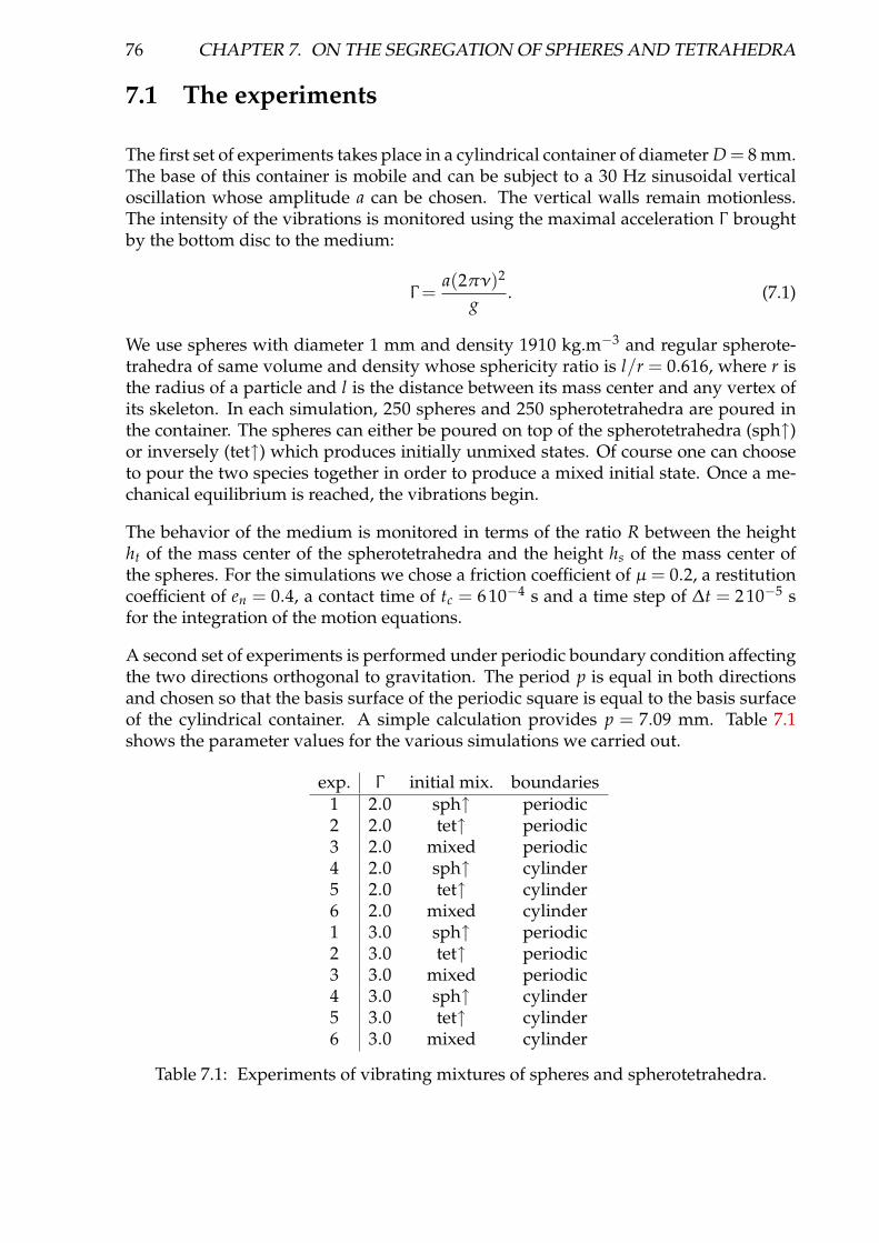
76 CHAPTER 7. ON THE SEGREGATION OF SPHERES AND TETRAHEDRA
7.1 The experiments
The first set of experiments takes place in a cylindrical container of diameter D = 8 mm.The base of this container is mobile and can be subject to a 30 Hz sinusoidal verticaloscillation whose amplitude a can be chosen. The vertical walls remain motionless.The intensity of the vibrations is monitored using the maximal acceleration Γ broughtby the bottom disc to the medium:
Γ =a(2πν)2
g. (7.1)
We use spheres with diameter 1 mm and density 1910 kg.m−3 and regular spherote-trahedra of same volume and density whose sphericity ratio is l/r = 0.616, where r isthe radius of a particle and l is the distance between its mass center and any vertex ofits skeleton. In each simulation, 250 spheres and 250 spherotetrahedra are poured inthe container. The spheres can either be poured on top of the spherotetrahedra (sph↑)or inversely (tet↑) which produces initially unmixed states. Of course one can chooseto pour the two species together in order to produce a mixed initial state. Once a me-chanical equilibrium is reached, the vibrations begin.
The behavior of the medium is monitored in terms of the ratio R between the heightht of the mass center of the spherotetrahedra and the height hs of the mass center ofthe spheres. For the simulations we chose a friction coefficient of µ = 0.2, a restitutioncoefficient of en = 0.4, a contact time of tc = 6 10−4 s and a time step of ∆t = 2 10−5 sfor the integration of the motion equations.
A second set of experiments is performed under periodic boundary condition affectingthe two directions orthogonal to gravitation. The period p is equal in both directionsand chosen so that the basis surface of the periodic square is equal to the basis surfaceof the cylindrical container. A simple calculation provides p = 7.09 mm. Table 7.1shows the parameter values for the various simulations we carried out.
exp. Γ initial mix. boundaries1 2.0 sph↑ periodic2 2.0 tet↑ periodic3 2.0 mixed periodic4 2.0 sph↑ cylinder5 2.0 tet↑ cylinder6 2.0 mixed cylinder1 3.0 sph↑ periodic2 3.0 tet↑ periodic3 3.0 mixed periodic4 3.0 sph↑ cylinder5 3.0 tet↑ cylinder6 3.0 mixed cylinder
Table 7.1: Experiments of vibrating mixtures of spheres and spherotetrahedra.

7.2. RESULTS AND DISCUSSION 77
Figure 7.1: . Lateral Snapshots of the initial (top row) and final (bottom row) situationsfor experiments 4, 5 and 6 (from left to right).
7.2 Results and discussion
Figure 7.2 shows the ratio R drawn against time for experiments 4, 5 and 6. One cansee that the initially homogeneously mixed state (experiment 6) does not segregate. Asa possible cause for this, one could invoke the intensity of the vibrations which is notsufficient to produce rearrangements. It is clear, however, that the initially unmixedstates (experiments 4 and 5) are unstable under those vibrations, meaning that therearrangements actually occur with this acceleration. Moreover, those rearrangementstend to mix spheres and spherotetrahedra.
Looking at figure 7.3, one can see that at the end of the experiments, most of the par-ticles about the cylinder boundary are spheres. This suggests that segregation indeedoccurs with mixtures of spheres and spherotetrahedra but in a radial way. Indeed, fig-ure 7.3 shows the proportion P of spheres among all the particles whose centers areat a distance less than l + r of the boundary. The proportion P of spheres reaches 0.8
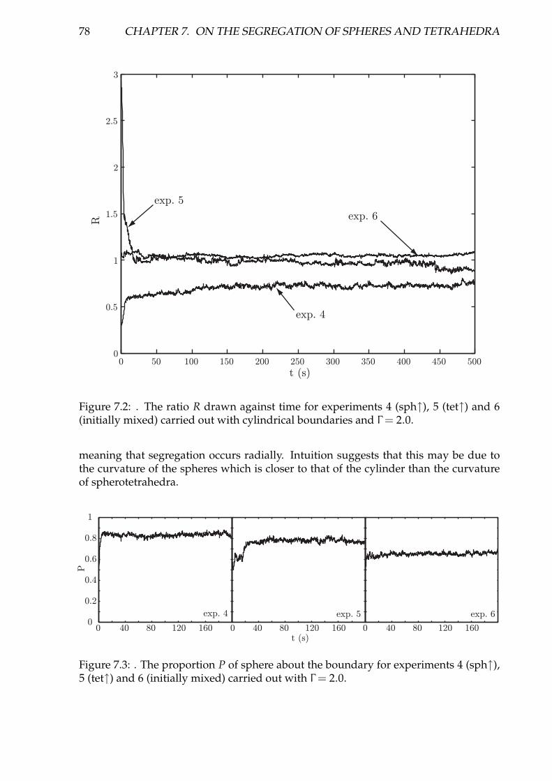
78 CHAPTER 7. ON THE SEGREGATION OF SPHERES AND TETRAHEDRA
0 50 100 150 200 250 300 350 400 450 5000
0.5
1
1.5
2
2.5
3
t (s)
R
exp. 5
exp. 6
exp. 4
Figure 7.2: . The ratio R drawn against time for experiments 4 (sph↑), 5 (tet↑) and 6(initially mixed) carried out with cylindrical boundaries and Γ = 2.0.
meaning that segregation occurs radially. Intuition suggests that this may be due tothe curvature of the spheres which is closer to that of the cylinder than the curvatureof spherotetrahedra.
0 40 80 120 1600
0.2
0.4
0.6
0.8
1
P
0 40 80 120 160t (s)
0 40 80 120 160
exp. 4 exp. 5 exp. 6
Figure 7.3: . The proportion P of sphere about the boundary for experiments 4 (sph↑),5 (tet↑) and 6 (initially mixed) carried out with Γ = 2.0.

7.2. RESULTS AND DISCUSSION 79
Experiments with periodic boundary conditions have the nice property that radial seg-regation will not occur in such setups. This allows to separate vertical mixing and ra-dial segregation. Figure 7.4 shows the ratio R drawn against time for experiments 1,2 and 3. As one can see, nothing happens. The initially mixed medium (experiment3), and the initially unmixed ones (experiments 1 and 2) remain unmixed. One wouldexpect that either mixing or segregation would occur under vibrations. This suggeststhat our vibrations are not strong enough to allow the medium to rearrange. With pe-riodic boundary conditions there will be no convection. The rearrangements then onlyrely on the size of the voids created by the agitation of the medium.
0 50 100 150 200 250 300 350 400 4500
0.5
1
1.5
2
2.5
3
t (s)
R
exp. 3
exp. 1
exp. 2
Figure 7.4: . The ratio R drawn against time for experiments 1 (sph↑), 2 (tet↑) and 3(initially mixed) carried out with periodic boundary conditions and Γ = 2.0.
The ratio R is drawn against time for experiments 7, 8 and 9 in figure 7.5. Those exper-iments are identical to experiments 1, 2, and 3 but with Γ = 3.0 instead of Γ = 2.0. Onecan see that the medium not only rearranges but also converges to a final state that isidentical in terms of mixing for all three experiments. This means that our spheres andspherotetrahedra have a clear affinity for mixing.
The ratio R is shown in figure 7.6 for experiments 10, 11 and 12 identical to experiments7, 8 and 9 except that the periodic boundary has been replaced with cylindrical ones.One can see that the grains mix as well. Again, the final situation do not depend on the

80 CHAPTER 7. ON THE SEGREGATION OF SPHERES AND TETRAHEDRA
0 10 20 30 40 50 60 70 80 90 1000
0.5
1
1.5
2
2.5
3
t (s)
R
exp. 8
exp. 7
exp. 9
Figure 7.5: . The ratio R drawn against time for experiments 7 (sph↑), 8 (tet↑) and 9(initially mixed) carried out with periodic boundary conditions and Γ = 3.0.
initial states. This homogenization is spectacular, since less than five seconds sufficeto reach the final mixed state. One sees on figure 7.2 that the homogenization was notas perfect in experiments 4, 5 and 6 as it is in experiments 10, 11 and 12. It seems thatwith Γ = 2.0, the agitation is not sufficient for a strong mixing to occur.
One can see that the final mix of experiments 7-12 is obtained with R slightly lowerthan 1. This means that the average height of spherotetrahedra is lower than thatof spheres in the final mixed situation. This may be caused by a greater geometricalaffinity of spherotetrahedra with the bottom plane. Indeed spherotetrahedra have flatsurfaces corresponding to the facet of their skeletons. Those flat surfaces may lie moreeasily on the bottom plane than spherical ones, just in the same way spheres gatherabout cylindrical boundaries in experiments 4, 5 and 6. Figure 7.7 shows the propor-tion P of spheres about the boundary of the cylinder for experiments 10, 11 and 12.One can see that the radial segregation is dramatically less marked than with loweragitation.

7.2. RESULTS AND DISCUSSION 81
0 5 10 15 20 25 30 35 40 45 500
0.5
1
1.5
2
2.5
3
t (s)
R
exp. 11
exp. 10
exp. 12
Figure 7.6: . The ratio R drawn against time for experiments 10 (sph↑), 11 (tet↑) and 12(initially mixed) carried out with cylindrical boundaries and Γ = 3.0.
0 100 200 300 400 5000 100 200 300 400 500t (s)
0 100 200 300 400 5000
0.2
0.4
0.6
0.8
1
P
exp. 10 exp. 11 exp. 12
Figure 7.7: . The proportion P of sphere about the boundary for experiments 10 (sph↑),11 (tet↑) and 12 (initially mixed) carried out with Γ = 3.0.

82 CHAPTER 7. ON THE SEGREGATION OF SPHERES AND TETRAHEDRA
7.3 Conclusion
We have shown that spheres and spherotetrahedra with same volume and density tendto mix under sufficiently strong vibrations. This constitutes a rather unexpected resultsince grains with different properties most of the time segregate when submitted tovibrations. Still these conclusions need to be further validated. In particular the sensi-bility of the process to the sphericity ratio l/r should be investigated as well as the dy-namics of the mixing in function of the agitation intensity. We suggest that this mixingbehavior may be linked to the fact that the inertia matrix of regular spherotetrahedrais that of a sphere, which has to be validated as well, for example with experimentsinvolving several other shapes (spherocylinders or spherotriangles to begin with). Theother interesting effect reported in this chapter is the radial segregation occuring incylinders. Spheres seem to have a greater affinity with the cylindrical boundaries thanspherotetrahedra. This may be due to the curvature of the spheres that is closer to thecurvature of the cylinder than that of the spherotetrahedra, which is still to be checkedby trying mixtures between particles with different curvatures like spherocylindersand spherotriangles.
Conclusion
The central result of this thesis is the generalization to non-spherical particles of thesimulation techniques developed by D. Müller [ML95; Mül96a] for discs and polygonsand J.-A. Ferrez [Fer01; FL02] for spheres. In particular, a description of a wide rangeof particle shapes was proposed, as well as an extension of molecular dynamics con-tact models to such particles. The other important issue that was addressed is that ofcontact detection between bodies with those shapes. A generalization of triangulation-based contact detection methods to non-spherical particles was proposed. The case ofconvex particle shapes was fully covered, while for non-convex particles a method fortracking contacts between two time steps still needs to be worked out. Finally, threeexperiments were investigated numerically that provide validations of the numericalmodel as well as new insights on the behavior of granular media. Below we sum upwhat has been achieved in each direction addressed in this thesis and propose possiblefuture developments.
The implementation was based on the existing code by J.-A. Ferrez whose evolution-ary structure showed to be convenient. The simulation code can now handle mixedpopulations of spherosimplices using generalized contact models and our linear com-plexity triangulation-based contact detection method. Developing the code to be ableto handle more general spheropolyhedra represents a challenge for future work. Thiswill involve redesigning the simulation environment as well as finding solutions tostore such shapes in all their generality.
The contact detection algorithm was mathematically proven to work in a wide rangeof situations. The particular cases of one covering sphere per particle and that of sphe-rocylinders covered by many spheres were especially addressed. In the former case,detecting contacts between arbitrary shaped bodies or between spheres has the samecomplexity. In numerical trials, the actual complexity was found to be nearly linearin the number of particles with a slope that increases with particle elongation. Thisreflects the fact that the number of possible contacts is higher for elongated particlesthan for round ones.
In addition to the original algorithm 1, the robust regularization algorithm 3 has beenimplemented that fixes a problem occurring in some practical cases. While the theo-retical convergence of this last algorithm is not proven, up to now, no case was everencountered in practice where the algorithm failed to converge. Hence it might alwaysbe the case that changing a non-regular triangulation into a regular one with the samevertex set can be done by only flipping illegal facets.

84 CONCLUSION
In this thesis it has been shown that the flip-graph of regular triangulations that share asame vertex set is connected. The general case that also includes non-regular triangu-lations in three dimensions remains open, though. The behavior of our regularizationalgorithm may point to a direction for further investigating the connectivity of the flip-graph in three dimensions.
With the help of the simulation code, several phenomena concerning various forms ofbehavior of granular media were studied. A first experiment about the flowability ofbead assemblies was performed both with real-world setups and numerical simula-tion. The results of those trials indicate that the distinct element method is appropriateto measure the flowability of monodisperse bead assemblies, thus that the proposednumerical models successfully capture the behavior of statical granular media. Thedependence of flowability on friction was investigated and found to decrease with in-creasing friction coefficients. Finally, according to numerical trials, the flowability ofhomogeneous bidisperse bead assemblies was found to depend only on their mass-average diameters. It is expected that future work on the influence of particle shape onflowability using our tools will disclose interesting features.
The second set of experiments was carried out with spherocylinders. Monodisperseassemblies of such particles were vibrated vertically inside a cylindrical container. Avertical reordering recalling a crystallization was observed that agrees with experi-mental observations. The reasons for this behavior have been discussed and while ourcylindrical boundaries probably play an important role, it is however very likely thatother causes are also responsible for this verticalization phenomenon.
The last set of experiments was designed to investigate the shape segregation in mix-tures of spheres and spherotetrahedra with same volume and density. Such mixtureswere vibrated in cylindrical containers and also with periodic boundary conditions.With cylindrical boundaries, radial segregation was found to occur while unexpect-edly, no vertical segregation was observed neither with cylindrical containers, norwith periodic boundaries. Starting from completely unmixed situations, spheres andspherotetrahedra would even mix and reach an homogeneous state that turns out tobe independent of the initial situation.
Such experiments with non-spherical particles should be followed by others, for webelieve that the behavior of granular media composed of non-spherical particles willlead to more interesting and unexpected findings. For shape-segregation alone, withthe current version of our simulation code, investigating other kinds of mixtures stillneeds to be done. The influence of boundary conditions is another field with manyopen questions. Radial segregation should be investigated with a larger range of par-ticle shapes and the boundary-driven shape-segregation may be related to the curva-ture of the confining boundaries. Observations on such experiments should lead togain precious insights on the behavior of granular media composed of particles witharbitrary shapes.
Bibliography
[AD99] S. Douady A. Daerr. Two types of avalanche behaviour in granular media.Nature, 399(6733):241–243, may 1999.
[ADS98] P. Alliez, O. Devillers, and J. Snoeyink. Removing degeneracies by perturb-ing the problem or the world. In Proc. 10th Canad. Conf. Comput. Geom.,1998. INRIA Research Report 3316, 1997.
[Alg01] Algorithmic Solutions Software GmbH. LEDA, a Library of Efficient Datatypes and Algorithms. http://www.algorithmic-solutions.com/, 2001.
[AR01] B. Andrade and S. Reinmann. Simulation d’amas de grains sphériques.Projet de semestre, EPFL-DMA, 2001.
[AT87] M. P. Allen and D. J. Tildesley. Computer simulation of liquids. ClarendonPress, Oxford, 1987.
[ATC03] C. R. A. Abreu, F. W. Tavares, and M. Castier. Influence of particle shapeon the packing and on the segregation of spherocylinders via monte carlosimulations. Powder Tech., 134:167, 2003.
[Aur87] F. Aurenhammer. Power diagrams: properties, algorithms and applica-tions. SIAM J. Comput., 16(1):78–96, 1987.
[Aur88] F. Aurenhammer. Improved algorithms for discs and balls using powerdiagrams. J. Algorithms, 9:151–161, 1988.
[Bag05] K. Bagi. An algorithm to generate random dense arrangements for discreteelement simulations of granular assemblies. Granular Matter, 7(1):31–43,2005.
[Bar94] G. C. Barker. Computer simulations of granular materials. In A. Mehta,editor, Granular Matter: An interdisciplinary approach. Springer-Verlag, 1994.
[BEG+99] J. Basch, J. Erickson, L. J. Guibas, J. Hershberger, and L. Zhang. Kinetic col-lision detection for two simple polygons. In Proc. 10th ACM-SIAM Sympos.Discrete Algorithms, pages 102–111, 1999.
[BEKR03] A. J. P. Breu, H. M. Ensner, C. A. Kruelle, and I. Rehberg. Reversing thebrazil-nut effect: Competition between percolation and condensation. Phys.Rev. Lett., 90(1):014302, jan 2003.

86 BIBLIOGRAPHY
[Ber99] R. Berger. Triangulations dynamiques en 3D avec LEDA. Projet desemestre, EPFL-DMA, 1999.
[Ber00] R. Berger. Simulation de la chute d’un bloc rocheux sur un remblai. Projetde semestre, EPFL-DMA, 2000.
[BGH97] J. Basch, L. J. Guibas, and J. Hershberger. Data structures for mobile data.In Proc. 8th ACM-SIAM Sympos. Discrete Algorithms, pages 747–756, 1997.
[BGSZ97] J. Basch, L. J. Guibas, C. D. Silverstein, and L. Zhang. A practical evaluationof kinetic data structures. In Proc. 13th ACM Symposium on ComputationalGeometry, pages 388–390, 1997.
[BGZ97] J. Basch, L. J. Guibas, and L. Zhang. Proximity problems on moving points.In Proc. 13th ACM Symposium on Computational Geometry, pages 344–351,1997.
[BK94] R. Barriuso and A. Knies. SHMEM User’s Guide for C (Rev. 2.2). Cray Re-search Inc., 1994.
[BKS99] P. Bakucz, G. Krause, and D. Stoyan. Force distribution in loaded planardisc systems. In L. Gaul and C. A. Brebbia, editors, Computational Methodsin Contact Mechanics IV, pages 273–282. WIT Press, Southampton/Boston,1999.
[BNK03] D. L. Blair, T. Neicu, and A. Kudrolli. Vortices in vibrated granular rods.Phys. Rev. E, 67(3):031303, 2003.
[BSV01] H. Brönnimann, S. Schirra, and R. Veltkamp. The CGAL Reference Manual.http://www.cgal.org/Manual/, 2001.
[BY95] J.-D. Boissonnat and M. Yvinec. Géométrie Algorithmique. Ediscience inter-national, Paris, 1995. Published in english as Algorithmic Geometry, Cam-bridge University Press, 1998.
[BY97] H. Bronnimann and M. Yvinec. Efficient exact evaluation of signs of deter-minants. In Proc. 13th Annu. ACM Sympos. Comput. Geom., pages 166–173,1997.
[CCC+97] R. Chandra, D. Chen, R. Cox, D. E. Maydan, N. Nedeljkovic, and J. M.Anderson. Data distribution support on distributed shared memory mul-tiprocessors. In Proc. SIGPLAN 97, 1997.
[Cla99] Ph. Claudin. La physique des tas de sable. EDP Sciences, 1999.
[Cle98] P. W. Cleary. Discrete element modelling of industrial granular flow appli-cations. TASK Quarterly, 2(3):385–415, 1998.
[CLM+95] P. Cignoni, D. Laforenzy, C. Montani, R. Perego, and R. Scopigno. Evalu-ation of parallelization strategies for an incremental Delaunay triangulatorin E3. Concurrency: Practice and Experience, 7(1):61–80, 1995.

BIBLIOGRAPHY 87
[CMPS93] P. Cignoni, C. Montani, R. Perego, and R. Scopigno. Parallel 3D Delaunaytriangulation. Computer Graphics Forum, 12(3):129–142, 1993.
[CS79] P. A. Cundall and O. D. L. Strack. A discrete numerical model for granularassemblies. Géotechnique, 29(1), 1979.
[CS99] P. W. Cleary and M. L. Sawley. Three-dimensional modelling of industrialgranular flows. In Second International Conference on CFD in the Minerals andProcess Industries. CSIRO, Melbourne, Australia, 1999.
[CSSC95] J. Carreira, L. M. Silva, J. G. Silva, and S. Chapple. Implementing VirtualShared Memories on MPI. In MPI Developers Conference, University of NotreDame, June 1995.
[Cun88] P. A. Cundall. Formulation of a three-dimensional distinct-element model— Part I. A scheme to detect and represent contacts in a system composedof many polyhedral blocks. Int. J. Rock Mech. Min. Sci. & Geomech. Abstr.,25(3), 1988.
[CW96] K. Chung and W. Weng. Quick collision detection of polytopes in virtualenvironments. In Proc. 3rd ACM Sympos. Virtual Reality Software and Tech-nology, pages 125–132, 1996.
[CWBC98] M. E. Cates, J. P. Wittmer, J.-P. Bouchaud, and P. Claudin. Development instresses in cohesionless poured sand. Phil. Trans. R. Soc. Lond. A, 356:2535–2560, 1998.
[DFM04] R. Dougherty, V. Faber, and M. Murphy. Unflippable tetrahedral com-plexes. Discrete Comput. Geom., 32:309–315, 2004.
[DGKS96] O. Devillers, M. Golin, K. Kedem, and S. Schirra. Queries on Voronoi dia-grams of moving points. Comput. Geom. Theory Appl., 6:315–327, 1996.
[DH97] A. C. Davison and D. V. Hinkley. Bootstrap Methods and Their Application.Cambridge University Press, 1997.
[DL89] D. P. Dobkin and M. J. Laszlo. Primitives for the manipulation of three-dimensional subdivisions. Algorithmica, 4:3–32, 1989.
[dLRS04] J. A. de Loera, J. Rambau, and F. Santos. Triangulations of point sets. Applica-tions, structures, algorithms. 2004. manuscript.
[dLSU99] J. A. de Loera, F. Santos, and J. Urrutia. The number of geometric bistellarneighbors of a triangulation. Discrete Comput. Geom., 21:131–142, 1999.
[DMO05] E. D. Demaine, J. S. B. Mitchell, and J. O’Rourke. The open problems page,problem 28. Web page stating the conjecture, http://maven.smith.edu/~orourke/TOPP/P28.html, 2005.
[Dos98] G. Dos Reis. Vers une nouvelle approche du calcul scientifique en C++.Technical Report RR-3362, INRIA, 1998. http://www.inria.fr/rrrt/rr-3362.html.

88 BIBLIOGRAPHY
[Dra91] T. G. Drake. Granular flow: physical experiments and their implicationsfor microstructural theories. J. Fluids. Mech., 12(225), 1991.
[DRC93] J. Duran, J. Rajchenbach, and E. Clément. Arching effect model for particle-size segregation. Phys. Rev. Lett., 70(16):2431–2434, apr 1993.
[DS00] Y. Dai and A. Sutou. A study of the global optimization approachto spherical packing problems. Technical Report B-361, Tokyo In-stitue of Technology, May 2000. http://www.is.titech.ac.jp/research/research-report/B/.
[Dur00] J. Duran. Sands, Powders, and Grains: An introduction to the Physics of Granu-lar Materials. Springer, 2000.
[Ede87] H. Edelsbrunner. Algorithms in Combinatorial Geometry. Springer-Verlag,1987.
[EGSZ99] J. Erickson, L. J. Guibas, J. Stolfi, and L. Zhang. Separation-sensitive colli-sion detection for convex objects. In Proc. 10th ACM-SIAM Sympos. DiscreteAlgorithms, pages 327–336, 1999.
[EM90] H. Edelsbrunner and E. P. Mücke. Simulation of simplicity: a technique tocope with degenerate cases in geometric algorithms. ACM Trans. Graph.,6:66–104, 1990.
[EPW90] H. Edelsbrunner, F. P. Preparata, and D. B. West. Tetrahedrizing point setsin three dimensions. J. Symbolic Comput., 10(3-4):335–347, 1990.
[ES96] H. Edelsbrunner and N. R. Shah. Incremental topological flipping worksfor regular triangulations. Algorithmica, 15:223–241, 1996.
[Fer01] J.-A. Ferrez. Dynamic Triangulations for Efficient 3D Simulation of GranularMaterials. Thèse N◦ 2432, EPFL, 2001.
[FFDH90] S. Feiner, J. Foley, A. Van Dam, and J. F. Hughes. Fundamentals of interactivecomputer graphics. Addison Wesley, USA, 2nd edition, 1990.
[FL00] J.-A. Ferrez and Th. M. Liebling. Using dynamic triangulations in distinctelement simulations. In M. Deville and R. Owens, editors, Proceedings of the16th IMACS World Congress, August 2000.
[FL02] J.-A. Ferrez and Th. M. Liebling. Dynamic triangulations for efficient de-tection of collisions between sheres with applications in granular mediasimulations. Phil. Mag. B, 82(8):905–929, 2002.
[FLCA94] S. F. Foester, M. Y. Louge, H. Chang, and K. Allia. Measurement of thecollision properties of small spheres. Phys. Fluids, 6(1108), 1994.
[FML00] J.-A. Ferrez, D. Müller, and Th. M. Liebling. Dynamic triangulations forgranular media simulations. In K. R. Mecke and D. Stoyan, editors, Statis-tical Physics and Spatial Statistics, Lecture Notes in Physics. Springer, 2000.
BIBLIOGRAPHY 89
[FV93] S. Fortune and Ch. J. Van Wyk. Efficient exact arithmetic for computationalgeometry. In Ninth Annual Symposium on Computational Geometry, pages163–172, 1993.
[GB90] J. Ghaboussi and R. Barbosa. Three-dimensionnal discrete element methodfor granular materials. Int J. for Numerical and Analytical Methods in Geome-chanics, 14(451), 1990.
[Gio80] A. Gioia. Intrinsic flowability: a new technology for powder-flowabilityclassification. Pharm. Tech., pages 65–68, february 1980.
[GKS92] L. J. Guibas, D. E. Knuth, and M. Sharir. Randomized incremental construc-tion of Delaunay and Voronoi diagrams. Algorithmica, 7:381–413, 1992.
[GKZ94] I. M. Gel’fand, M. M. Kapranov, and A. V. Zelevinsky. Discriminants, resul-tants, and multidimensional determinants, Mathematics: Theory & Applications.Birkhäuser, Boston, 1994.
[GMR91] L. Guibas, J. S. B. Mitchell, and T. Roos. Voronoi diagrams of moving pointsin the plane. In Proc. 17th Internat. Workshop Graph-Theoret. Concepts Comput.Sci., volume volume 570 of Lecture Notes in Computer Science, pages 113–125. Springer-Verlag, 1991.
[Gol91] D. Goldberg. What every computer scientist should know about floating-point arithmetic. ACM Computing Surveys, 23(1):5–48, 1991.
[GS85] L. Guibas and J. Stolfi. Primitives for the manipulation of general subdi-visions and the computation of Voronoi diagrams. ACM Transactions onGraphics, 4(2):74–123, 1985.
[GZ98] L. J. Guibas and L. Zhang. Euclidean proximity and power diagrams. InProc. 10th Canadian Conference on Computational Geometry, 1998.
[GZK90] I. M. Gel’fand, A. V. Zelevinskii, and M. M. Kapranov. Discriminants ofpolynomials of several variables and triangulations of newton polyhedra.Leningrad Math J., 2:449–505, 1990.
[HKBS96] B. P. B. Hoomans, J. A. M. Kuipers, W. J. Briels, and W. P. M. Van Swaaij. Dis-crete particle simulation of bubble and slug formation in a two-dimensionalgas-fluidised bed: a hard-sphere approach. Chemical Engineering Science,51(1):99–118, 1996.
[HQL01] D. C. Hong, P. V. Quinn, and S. Luding. Reverse brazil nut prob-lem: Competition between percolation and condensation. Phys. Rev. Lett.,86(15):3423–3426, apr 2001.
[HSS83] J. E. Hopcroft, J. T. Schwartz, and M. Sharir. Efficient detection of intersec-tions among spheres. Intl. J. Robotics Research, 2(4):77–80, 1983.
[IIM85] H. Imai, M. Iri, and K. Murota. Voronoi diagram in the Laguerre geometryand its applications. SIAM J Computing, 14(1):93–105, 1985.
90 BIBLIOGRAPHY
[Ind95] C. Indermitte. Modélisation et simulation de la croissance d’un mycélium. ThèseN◦ 1404, EPFL, 1995.
[Joe89] B. Joe. Three-dimensional triangulations from local transformations. SIAMJ. Sci. Stat. Comput., 10(4):718–741, 1989.
[Joe91] B. Joe. Construction of three-dimensional Delaunay triangulations usinglocal transformations. Computer Aided Geometric Design, 8:123–142, 1991.
[Joe92] B. Joe. Three-dimensional boundary-constrained triangulations. In E. N.Houstis and J. R. Rice, editors, Artificial Intelligence, Expert Systems, andSymbolic Computing, pages 215–222. Elsevier Science Publishers, 1992. ftp://ftp.cs.ualberta.ca/pub/geompack/Papers/Joe92.ps.Z.
[Joe93] B. Joe. Construction of k-dimensional Delaunay triangulations using localtransformations. SIAM J. Sci. Comput., 14(6):1415–1436, 1993.
[Joe95] B. Joe. Construction of three-dimensional improved-quality triangulationsusing local transformations. SIAM J. Sci. Comput., 16:1929–1307, 1995.
[Joh85] K.L. Johnson. Contact Mechanics. Cambridge Univ. Press, New York, 1985.
[JS83] J. T. Jenkins and S. B. Savage. A theory for the rapid flow of identical,smooth, nearly elastic, spherical particles. J Fluid Mech, 130:187–202, 1983.
[KG99] P. Kuonen and R. Gruber. Parallel computer architectures for commod-ity computing and the Swiss-T1 machine. EPFL Supercomputing Review,11, 1999. Online at http://sawww.epfl.ch/SIC/SA/publications/SCR99/scr11-page3.html.
[KJN93] J. B. Knight, H. M. Jaeger, and S. R. Nagel. Vibration-induced size sep-aration in granular media - the convection connection. Phys. Rev. Lett.,70(24):3728–3731, jun 1993.
[KK87] G. Kuwabara and K. Kono. Restitution coefficient in a collision betweentwo spheres. Jap. J. Appl. Phys., 26(1230), 1987.
[KMZ91] W. Kurz, J. P. Mercier, and G. Zambelli. Introduction à la Science des Matéri-aux, volume 1 of Traité des Matériaux. Presses Polythechniques et Universi-taires Romandes, 2ème edition, 1991.
[Law77] C. L. Lawson. Mathematical Software III, chapter Software for C1 interpola-tion. Academic Press, New York, 1977.
[LCB+94] S. Luding, E. Clément, A. Blumen, J. Rajchenbach, and J. Duran. Anoma-lous energy dissipation in molecular-dynamics simulations of grains: The"detachment" effect. Phys. Rev. E, 50(4113), 1994.
[LDCR05] S. Luding, J. Duran, E. Clément, and J. Rajchenbach. Simulations of densegranular flow: Dynamic arches and spin organization. J. Phys. I, 6(6):823–836, 2005.
BIBLIOGRAPHY 91
[LL90] F. Lamarche and C. Leroy. Evaluation of the volume of intersection of asphere with a cylinder by elliptic integrals. Computer Phys. Comm., 59:359–369, 1990.
[LMB92] J. Levine, T. Mason, and D. Brown. lex & yacc. O’Reilly, 2nd edition, 1992.
[LMT+92] Th. M. Liebling, A. Mocellin, H. Telley, F. Righetti, H. Clémençon, and C. In-dermitte. Nouvelles approches dans la modélisation et simulation de pro-cessus de croissance en science des matériaux et en biologie. Cahiers duCERO, 34:117–138, 1992.
[LNS+95] C. H. Liu, S. R. Nagel, D. A. Schecter, S. Majumdar, O. Narayan, and T. A.Witten. Force fluctuations in bead packs. Science, 269(5223):513–515, jul1995.
[LRD97] L. Labous, A. D. Rosato, and R. N. Dave. Measurements of collisional prop-erties of spheres using high-speed video analysis. Phys. Rev. E, 56(5717),1997.
[Mak97] H. A. Makse. Stratification instability in granular flows. Phys. Rev. E,56(6):7008–7016, dec 1997.
[Man88] M. Mantyla. An introduction to solid modeling. Computer Science Press, USA,1988.
[MC95] B. Mirtich and J. Canny. Impulse-based dynamic simulation, The agorithmicFoundations of robotics. A. K. Peters, 1995.
[MD98] S.-A. Magnier and F. V. Donzé. Numerical simulation of impacts using adiscrete element method. Mech. Cohes.-frict. Mater., 3, 1998.
[Mei01] E. Meichtry. Simulation d’amas de grains sphériques. Projet de semestre,EPFL-DMA, 2001.
[MEL05] B. Muth, P. Eberhard, and S. Luding. Collisions between particles of com-plex shapes. In R. García-Rojo, H. J. Herrmann, and S. McNamara, editors,Powders and Grains 2005, volume II, pages 1379–1383. A.A.Balkema, 2005.
[Mir97] B. Mirtich. V-clip: Fast and robust polyedral collision detection. TechnicalReport TR-97-05, Mitsubishi Electrical Research Laboratory, 1997.
[ML95] D. Müller and Th. M. Liebling. Detection of collisions of polygons by usinga triangulation. In M. Raous et al., editor, Contact Mechanics, pages 369–372.Plenum Publishing Corporation, New York, 1995.
[MLH00] H.-G. Matuttis, S. Luding, and H. J. Herrmann. Discrete element methodsfor the simulation of dense packings and heaps made of spherical and non-spherical particles. Powder Technology, 109(1-3):278–292, 2000.
[MLNJ01] M. E. Mobius, B. E. Lauderdale, S. R. Nagel, and H. M. Jaeger. Brazil-nut ef-fect - size separation of granular particles. Nature, 414(6861):270, nov 2001.
92 BIBLIOGRAPHY
[MMEL04] B. Muth, M.-K. Müller, P. Eberhard, and S. Luding. Contacts between manybodies. Machine Dynamics Problems, 28(1):101–114, 2004.
[MN99a] P. McCullagh and J. A. Nelder. Generalized Linear Models. Chapman andHall/CRC, second edition edition, 1999.
[MN99b] K. Mehlhorn and S. Näher. LEDA. Cambridge University Press, 1999.
[Mon92] J. J. Monaghan. Smoothed particle hydrodynamics. Annu. Rev. Astron. As-trophys., 30:543–574, 1992.
[Mon98] S. Montani Stoffel. Sollicitation dynamique de la couverture des galeries de pro-tection lors de chutes de blocs. Thèse N◦ 1899, EPFL, 1998.
[MP00] E Meichtry and S. Paroz. Animations interactives de triangulations 3D.Projet de semestre, EPFL-DMA, 2000.
[MTT00] Y. Muguruma, T. Tanaka, and Y. Tsuji. Numerical simulation of particulateflow with liquid bridge between particles (simulation of centrifugal tum-bling granulator). Powder Technology, 109:49–57, 2000.
[Mül96a] D. Müller. Techniques informatiques efficaces pour la simulation de mileux gran-ulaires par des méthodes d’éléments distincts. Thèse N◦ 1545, EPFL, 1996.
[Mül96b] D. Müller. Web page with example simulations of granular media. http://rosowww.epfl.ch/dm/sigma.html, 1996.
[Mül98] D. Müller. Mieux comprendre les milieux granulaires. IAS Bulletin, 9, 1998.
[MY92] S. McNamara and W. R. Young. Inelastic collapse and clumping in a one-dimensional granular medium. Phys. Fluids A, 4(496), 1992.
[MY96] S. McNamara and W. R. Young. Dynamics of a freely evolving, two-dimensional granular medium. Phys. Rev. E, 53(5):5089–5100, may 1996.
[Müc93] E. Mücke. Shapes and Implementations in Three-Dimensional Geometry. PhDthesis, Department of Computer Science, University of Illinois at Urbana-Champaign, 1993. Technical Report UIUCDCS-R-93-1836, ftp://cs.uiuc.edu/pub/TechReports/UIUCDCS-R-93-1836.ps.Z.
[ND94] T.-T. Ng and R. Dorby. Numerical simulations of monotonic and cyclicloading of granular soil. J. of Geotechnical Engineering, 120(338), 1994.
[NSK03] M. A. Naylor, M. R. Swift, and P. J. King. Air-driven brazil nut effect. Phys.Rev. E, 68(1):012301, jul 2003.
[O’C96] R. M. O’Connor. A distributed discrete element modeling environment - Algo-rithms, implementation and applications. PhD thesis, MIT, 1996.
[PB95] T. Pöschel and V. Buchholtz. Molecular dynamics of arbitrary shaped gran-ular particles. J. Phys. I, 5(1431), 1995.

BIBLIOGRAPHY 93
[PL05a] L. Pournin and Th. M. Liebling. A generalization of distinct elementmethod to tridimensional particles with complex shapes. In R. García-Rojo,H. J. Herrmann, and S. McNamara, editors, Powders and Grains 2005, vol-ume II, pages 1375–1378. A.A.Balkema, 2005.
[PL05b] L. Pournin and Th. M. Liebling. Monotone paths in the flip-graph of regulartriangulations. Submitted, 2005.
[PLM02] L. Pournin, Th. M. Liebling, and A. Mocellin. Molecular-dynamics forcemodels for better control of energy dissipation in numerical simulations ofdense granular media. Phys. Rev. E, 65:011302, 2002.
[Pou99] L. Pournin. Triangulations dynamiques pour la simulation de milieux gran-ulaires. Projet de diplôme, EPFL-DMA, 1999.
[PRFL05] L. Pournin, M. Ramaioli, P. Folly, and Th. M. Liebling. A law for the flowa-bility of bead assemblies. Submitted, 2005.
[Pri91] D. M. Priest. Algorithms for arbitrary precision floating point arithmetic.In P. Kornerup and D. Matula, editors, Tenth Symposium on Computer Arith-metic, pages 132–143. IEEE Computer Society Press, 1991.
[PWT+05] L. Pournin, M. Weber, M. Tsukahara, J.-A. Ferrez, M. Ramaioli, and Th. M.Liebling. Three-dimensional distinct element simulation of spherocylindercrystallization. Granular Matter, 7(2–3):119–126, 2005.
[Ramar] J. Rambau. On a generalization of schönhardt’s polyhedron. MSRI-Preprint2003-013, to appear.
[Rig92] F. Righetti. Modélisation 3D d’amas polycristallins et méthodologie et méthodolo-gie d’analyse de leurs images microscopiques. Thèse N◦ 1016, EPFL, 1992.
[Ris00] G. H. Ristow. Pattern formation in Granular Materials. Springer Tracts inModern Physics. Springer, 2000.
[RJMR96] F. Radjai, M. Jean, J.-J. Moreau, and S. Roux. Force distributions in densetwo-dimensional granular systems. Phys. Rev. Lett., 77(2):274–277, July1996.
[Rog85] D. Rogers. Procedural Elements for Computer Graphics. McGraw Hill, 1985.
[RPL05a] M. Ramaioli, L. Pournin, and Th. M. Liebling. Numerical and experimen-tal investigation of alignment and segregation of vibrated granular mediacomposed of rods and spheres. In R. García-Rojo, H. J. Herrmann, andS. McNamara, editors, Powders and Grains 2005, volume II, pages 1359–1363,Rotterdam, 2005. A.A.Balkema.
[RPL05b] M. Ramaioli, L. Pournin, and Th. M. Liebling. Why rods align verticallyunder vertical vibrations. Submitted, 2005.
94 BIBLIOGRAPHY
[RSPS87] A. Rosato, K. J. Strandburg, F. Prinz, and R. H. Swendsen. Why the brazilnuts are on top - size segregation of particulate matter by shaking. Phys.Rev. Lett., 58(10):1038–1040, mar 1987.
[RTLM03] M. Rhodes, S. Takeuchi, K. Liffman, and K. Muniandy. The role of intersti-tial gas in the brazil nut effect. Granular Matter, 5(3):107–114, dec 2003.
[Sam84] H. Samet. The quadtree and related hierarchical data structures. ACMComputing Surveys, 16:187–260, 1984.
[San00a] F. Santos. A point configuration whose space of triangulations is discon-nected. J. Amer. Math. Soc., 13(3):611–637, 2000.
[San00b] F. Santos. Triangulations with very few geometric bistellar neighbors. Dis-crete Comput. Geom., 23:15–33, 2000.
[SCB90] R. Sondergaard, K. Caney, and C. E. Brennen. Measurements of solidspheres bouncing off flat plates. ASME J. Appl. Mech., 57(694), 1990.
[Sch28] E. Schönhardt. Über die zerlegung von dreieckspolyedern in tetraeder.Math. Ann., 98:309–312, 1928.
[Sch99] A. Schinner. Fast algorithms for the simulation of polygonal particles. Gran-ular Matter, 2(1):35–43, 1999.
[SDW96] J. Schäfer, S. Dippel, and D. E. Wolf. Force schemes in simulations of gran-ular materials. J. Phys. I, 6(5), 1996.
[She96] J. R. Shewchuk. Robust adaptive floating-point geometric predicates. InProceedings of the Twelfth Annual Symposium on Computational Geometry.ACM, 1996. http://www.cs.cmu.edu/~quake/robust.html.
[She97] J. R. Shewchuk. Adaptive precision floating-point arithmetic and fast ro-bust geometric predicates. Discrete & Computational Geometry, 18:305–363,1997. http://www.cs.cmu.edu/~quake/robust.html.
[She05] J. R. Shewchuk. General-dimensional constrained delaunay and con-strained regular triangulations i: Combinatorial properties. To appear inDiscrete and Computational Geometry, 2005. Available online at http://www.cs.cmu.edu/~jrs/jrspapers.html#cdt.
[Shi04] T. Shinbrot. Granular materials - the brazil nut effect - in reverse. Nature,429(6990):352–353, may 2004.
[SM98] T. Shinbrot and F. J. Muzzio. Reverse buoyancy in shaken granular beds.Phys. Rev. Lett., 81(20):4365–4368, nov 1998.
[SOB92] K. Sugihara, A. Okabe, and B. Boots. Spatial Tesselations — Concepts andApplications of Voronoi Diagrams. John Wiley, 1992.
[SSW00] H. Sigurgeirsson, A. Stuart, and W.-L. Wan. Collision detection for particlesin a flow. http://www.maths.warwick.ac.uk/~stuart/hersir2.ps, 2000.
BIBLIOGRAPHY 95
[Str97] B. Stroustrup. The C++ Programming Language. Addison Wesley, 3rd edition,1997.
[STS93] M. H. Sadd, Q. Tai, and A. Shukla. Contact law effects on wave propagationin particulate materials using distinct element modeling. Int. J. Non-LinearMechanics, 28(251), 1993.
[Tel89] H. Telley. Modélisation et simulation bidimensionnelle de la croissance des poly-cristaux. Thèse N◦ 780, EPFL, 1989.
[The01] The CGAL Team. CGAL, Computational Geometry Algorithm Library.http://www.cgal.org/, 2001.
[TLM96a] H. Telley, Th. M. Liebling, and A. Mocellin. The Laguerre model of graingrowth in two dimensions: Part I. Cellular structures viewed as dynamicalLaguerre tesselations. Phil. Mag. B, 73(3):395–408, 1996.
[TLM96b] H. Telley, Th. M. Liebling, and A. Mocellin. The Laguerre model of graingrowth in two dimensions: Part II. Examples of coarsening simulations.Phil. Mag. B, 73(3):409–427, 1996.
[TSBP93] Y. A. Teng, F. Sullivan, I. Beichl, and E. Puppo. A data-parallel algorithmfor the three-dimensional Delaunay triangulation and its implementation.In Proceedings of Supercomputing ’93, Portland, Oregon, pages 112–121, 1993.
[Tsu03] M. Tsukahara. Simulations numériques de milieux granulaires avec desgrains cylindriques. Projet de diplôme, EPFL-SB-IMA-ROSO, 2003.
[VLMJ00] F. X. Villarruel, B. E. Lauderdale, D. M. Mueth, and H. M. Jaeger. Com-paction of rods : Relaxation and ordering in vibrated, anisotropic granularmaterial. Phys. Rev. E, 61(6):6914, 2000.
[WB86] O. R. Walton and R. L. Braun. Viscosity, granular-temperature, and stresscalculations for shearing assemblies of inelastic, frictional discs. J. of Rheol-ogy, 30(949), 1986.
[WB93] O. Wenzel and N. Bicanic. A quad tree based contact detection algorithm.In Proceedings of the 2nd international conference on discrete element methods(DEM), MIT. IESL Publications, 1993.
[Wei00] Ch. Weibel. Parallélisation d’un algorithme de simulation de milieux gran-ulaires. Projet de diplôme, EPFL-DMA, 2000.
[XRT+97] X. Xue, F. Righetti, H. Telley, Th. M. Liebling, and A. Mocellin. The Laguerremodel for grain growth in three dimensions. Phil. Mag. B, 75(4):567–585,1997.
[Xue95] X. Xue. Laguerre models for grain growth. Thèse N◦ 1466, EPFL, 1995.


Lionel Pournin rosowww.epfl.ch/lpBorn December 22, 1975 [email protected]
EDUCATION1999 – 2005 École Polytechnique Fédérale de Lausanne, Lausanne, Switzerland: www.epfl.ch
PhD student in Operations Research, Institute of Mathematics,under the supervision of Prof. Th. M. Liebling.Thesis subject: "on the behavior of spherical and non-spherical grain assemblies,its modeling and numerical simulation".
1996 – 1999 École Nationale Supérieure des Mines de Nancy, Nancy, France: mines.u-nancy.frEngineering degree obtained june 1999,(Diplôme d’ingénieur civil des Mines de Nancy).Master equivalent degree in materials science obtained september 1999,(DEA de science et ingénieurie des materiaux).
1997 – 1998 Henri Poincaré University (Nancy II), Nancy, France: www.uhp-nancy.frBachelor equivalent degree in mathematics obtained june 1998,(Maîtrise de mathématiques).
1993 – 1996 Lycée Chaptal, Paris, France: www.lycee-chaptal-paris.comClasses préparatoires de mathématiques supérieures et spéciales M’.
1990 – 1993 Lycée Honoré de Balzac, Mitry-Mory, France:Baccalauréat C (scientific) obtained june 1993.
PROFESSIONAL EXPERIENCE2005 – 2006 EPFL – Institute of Mathematics, Lausanne: roso.epfl.ch/cours/rosc/hiver05-06/
Lecturer of the operations research course for 5th semester studentsin Communication Systems, winter semester.
1999 – 2005 EPFL – Institute of Mathematics, Lausanne: roso.epfl.ch/lp/teaching.htmlAssistant of Prof. Th. M. Liebling, chair of Operations Research.
PUBLICATIONS2005 L. Pournin, M. Weber, M. Tsukahara, J.-A. Ferrez, M. Ramaioli, Th. M. Liebling, Three-dimensional
distinct element simulation of spherocylinder crystallization,Granular Matter 7, 2-3, 119-126 (2005).
2002 L. Pournin, Th. M. Liebling, and A. Mocellin, Molecular-dynamics force models for better control ofenergy dissipation in numerical simulations of dense granular media,Phys. Rev. E 65, 011302 (2002).
VARIOUSLanguages: Fluent in French and English, good knowledge of Romanian, basic knowledge of German.
CAE (Cambridge Certificate in Advanced English) obtained december 1997.ZDAF (Zertifikat Deutsch als Fremdsprache) obtained march 1999.


![Le gueux philosophe (Jean-Jacques Rousseau) [Jerôme Meizoz]](https://img.dokumen.tips/doc/110x75/62abae94bf37e0572474ab5f/le-gueux-philosophe-jean-jacques-rousseau-jerme-meizoz.jpg)