Embed Size (px)
Citation preview

On the axioms of scale space theory
Citation for published version (APA):Duits, R., Florack, L. M. J., Graaf, de, J., & Haar Romenij, ter, B. M. (2004). On the axioms of scale spacetheory. Journal of Mathematical Imaging and Vision, 20(3), 267-298.https://doi.org/10.1023/B:JMIV.0000024043.96722.aa
DOI:10.1023/B:JMIV.0000024043.96722.aa
Document status and date:Published: 01/01/2004
Document Version:Publisher’s PDF, also known as Version of Record (includes final page, issue and volume numbers)
Please check the document version of this publication:
• A submitted manuscript is the version of the article upon submission and before peer-review. There can beimportant differences between the submitted version and the official published version of record. Peopleinterested in the research are advised to contact the author for the final version of the publication, or visit theDOI to the publisher's website.• The final author version and the galley proof are versions of the publication after peer review.• The final published version features the final layout of the paper including the volume, issue and pagenumbers.Link to publication
General rightsCopyright and moral rights for the publications made accessible in the public portal are retained by the authors and/or other copyright ownersand it is a condition of accessing publications that users recognise and abide by the legal requirements associated with these rights.
• Users may download and print one copy of any publication from the public portal for the purpose of private study or research. • You may not further distribute the material or use it for any profit-making activity or commercial gain • You may freely distribute the URL identifying the publication in the public portal.
If the publication is distributed under the terms of Article 25fa of the Dutch Copyright Act, indicated by the “Taverne” license above, pleasefollow below link for the End User Agreement:www.tue.nl/taverne
Take down policyIf you believe that this document breaches copyright please contact us at:[email protected] details and we will investigate your claim.
Download date: 14. May. 2020

Journal of Mathematical Imaging and Vision 20: 267–298, 2004c© 2004 Kluwer Academic Publishers. Manufactured in The Netherlands.
On the Axioms of Scale Space Theory
REMCO DUITS, LUC FLORACK, JAN DE GRAAF AND BART TER HAAR ROMENYEindhoven University of Technology, Den Dolech 2, NL-5600 MB, The Netherlands
Abstract. We consider alternative scale space representations beyond the well-established Gaussian case thatsatisfy all “reasonable” axioms. One of these turns out to be subject to a first order pseudo partial differentialequation equivalent to the Laplace equation on the upper half plane {(x, s) ∈ Rd × R | s > 0}. We investigate thisso-called Poisson scale space and show that it is indeed a viable alternative to Gaussian scale space. Poisson andGaussian scale space are related via a one-parameter class of operationally well-defined intermediate representationsgenerated by a fractional power of (minus) the spatial Laplace operator.
Keywords: Gaussian scale space, Poisson scale space, α scale spaces, scale space axiomatics, semigroup theory
1. Introduction
Constructions of linear scale space representationsbased on rigorous axiomatics date back to the 1960’swith the publications by Iijima [22, 23] in the con-text of pattern recognition. This early work was fol-lowed by numerous publications [1, 11, 19, 24–30, 36]. The pivot in all derivations is some setof axioms expressing desirable group and/or semi-group properties. For an overview cf. Weickert[38].
It is commonly taken for granted that the Gaussianscale space paradigm is the unique solution to a setof reasonable axioms if one disregards minor modifi-cations, such as spatial inhomogeneities [12], diffeo-morphisms [13, 14], and anisotropies [37], which canbe easily accounted for. That this is in fact not truehas been pointed out by Pauwels [30], who proposeda one-parameter class of scale space filters in Fourierspace, which are compatible with some basic axioms.1
Under the assumption of positivity the correspondingparameter domain is a finite interval α ∈ (0, 1], whereα = 1/2 and α = 1 the correspond to Poisson, respec-tively Gaussian scale space.
In this article we scrutinize properties of theseα scalespaces (and in particular Poisson scale space) in thespatial domain, and show that they indeed obey all basicaxioms initially believed to hold only for the Gaussiancase.2 To demonstrate this we adopt an overcompleteset of axioms that capture the various subsets that havebeen employed in the derivation of the Gaussian scalespace paradigm. In addition, some of the conjecturesraised by Pauwels [30] are verified by rigorous proofs,whereas some intuitive expectations are disproved. Forexample, it turns out that, contrary to previous belief,the Fourier filters for all parameter values, includingthe Poisson filter, do possess infinitesimal generatorsin the spatial domain in the sense of linear derivativeoperators.
The most natural case of all α scale spaces is thePoisson scale space since it is the only one where thescale parameter has the same physical dimension asthe spatial variables xi , allowing Euclidean geome-try within scale space. Moreover, its Clifford analyticextension, which is first introduced in a computer vi-sion context by Felsberg and Sommer [9] has severalpractical benefits. Initially, Felsberg and Duits workedindependently on the subject of Poisson scale space

268 Duits et al.
following a different approach, but recently a cooper-ation has started on the subject of finite domain scalespaces, cf. [5, 8] which will not be considered in thisarticle. In this article Poisson scale space is shown tobe associated with the first order linear scale spacepseudo p.d.e.
∂u
∂s= −√−� u,
which at the same time illustrates the cause of previousfailure, viz. the fact that the possibility of a genera-tor in the form of a fractional power of a derivativeoperator—the precise definition of which will be out-lined in this article—has been overlooked. The solutionof this equation for initial condition f is neverthelessa perfectly viable, smooth scale space image, whichis essentially different from its Gaussian counterpart.The solution can in fact be written as a straightfor-ward convolution in closed-form using Poisson filters.Just like filtering with Gaussian kernels is equivalent tosolving the diffusion equation on the upper half space,filtering with Poisson kernels is equivalent to solvingthe Dirichlet problem on the upper half space. Finally,we establish an explicit connection between the vari-ous scale space representations, in particular Poissonand Gaussian scale spaces. Although we will not fo-cus explicitly on probability theory in this article, wewould like to mention that α-scale spaces correspondto α-stable Levy motions in the field of stochastic3
processes [34].
2. Preliminaries and Notation
A point in scale space Rd × R+ will be denoted by(x, s). Sometimes (if scale is fixed) we will write x forshort. Let a ∈ Rd and λ ∈ R and define �λ, Sλ, Ta by
[�λ f ](x) = f (x/λ)
[Sλ f ](x) = λ f (x) (1)
[Ta f ](x) = f (x − a)
Let�be a subset of Rd , then �denotes the closure of�.The boundary of � which equals �\� will be denotedby ∂�. The outward normal to the boundary will bewritten n. The d-dimensional ball in Rd with respect tothe Euclidean metric, with center a and radius R > 0,will be denoted by Ba,R . The total surface measure of∂ Ba,R equals σd Rd−1. From
∫Rd e−‖x‖2
dx = πd/2, it
easily follows that
σd = 2 (π )d2
(d/2). (2)
In the 1D case, d = 1, we occasionally use complexfunction theory. We then use the following notationz = x + is = reiθ . We denote the real respectivelyimaginary part of a complex number w by �(w) re-spectively �(w).
With regard to spaces we use the following notation:
• L(X, Y ) = the vector space consisting of linear op-erators from X into Y . If X = Y we write L(X ) forshort.
• B(X, Y ) = the vector space consisting of continuouslinear operators from X into Y . If X = Y we writeB(X ) for short.
• If A ∈ B(X ), with spectrum σ (A), then its resolventis defined by
R(λ;A) = (λI − A)−1.
for all λ ∈ ρ(A) = C \ σ (A).• The dual of a vector space X is the vector space
consisting of all continuous linear functionals on Xand will be denoted by X ′.
• Lp(�, µ) = the quotient space consisting of func-tions with finite L p norm (p > 0), i.e.(∫�
| f |p dµ)1/p < ∞ on � with respect to the nilspace of the L2-norm, which consists of all functionsf on � with zero measure support, i.e. f = 0 almosteverywhere. Mostly µ equals the usual Lebesguemeasure md and then we write Lp(�) for short.
• The Fourier transform F : L2(Rd ) → L2(Rd ), is(A.E.) defined by
[F( f )](ω) = 1
(2π )d/2
∫Rd
f (x) e−iω·x dx,
mostly we will write f in stead of F( f ).• The Laplace transform4 L( f ) of a function f ∈
L2(R+) is defined by
[L( f )](λ) =∫ ∞
0f (x) e−λx dx,
for �(λ) > 0.• Associate to each s > 0 a positive measure µs , by
setting
dµs(y) = (1 + ‖y‖2)s dmd (y) s > 0 (3)

On the Axioms of Scale Space Theory 269
• Cn(�) = the vector space consisting of all n timescontinuous differentiable functions on �.
• D(�) = the vector space consisting of all in-finitely differentiable functions with compact sup-port within �. This space is equipped with the lo-cal convex topology generated by the semi-normsqN : D(�) → R (N ∈ N) given by
qN ( f ) = sup|α|<N
sup‖x‖<N
|(Dα f )(x)|
• Define the semi-norms pN : C∞(Rd ) → R (N ∈ N)by
pN ( f ) = sup|α|<N
supx∈Rd
(1 + ‖x‖2)N |(Dα f )(x)|.
• Sd = the vector space consisting of all infinitely dif-ferentiable function f such that pN ( f ) < ∞ for allN ∈ N. This space is equipped with the local convextopology generated by the semi-norms pN . The ele-ments in the dual space S ′
d are often called tempereddistributions. The Fourier transform of a tempereddistribution is defined5 by (φ) = (φ).
• Hs(Rd ) equals the vector space consisting of all tem-pered distributions which Fourier transform is inL2(Rd ; µs).
The kernels Gs : Rd → R, Hs : Rd → R are definedby
Gs(x) = 1
(4πs)d/2e− ‖x‖2
4s
Hs(x) = 2
σd+1
s
(s2 + ‖x‖2)d+1
2
.
(4)
Note that Gs is a rapidly decreasing function while Hs isnot. This means that the distributional approach to scalespace theory cf. [11], regarding raw images as distri-butions defined on the test space of rapidly decreasingfunctions, needs some adaptation for other semigroupssuch as Poisson filtering (see Appendix).
The mapping from the original image f and scale sonto the blurred image will be denoted by � : L2(Rd )×R+ → L2(Rd ). The blurred image at a fixed scale s > 0will be denoted by u and is given by
u(x, s) = �[ f, s](x), x ∈ Rd
In order to stress that s > 0 is fixed, we will often write�s f in stead of �[ f, s].
3. Axioms
First we will summarize some basic observations withrespect to blurring:
• If the scale s tends to zero, the blurred image musttend to the original image. For continuous imagesthis convergence must be pointwise.
• If two images f1, f2 satisfy f1(x) ≤ f2(x) almosteverywhere on Rd , then the corresponding blurredimages u1, u2 must satisfy u1(x, s) ≤ u2(x, s) almosteverywhere on Rd for all s > 0.
• Successive blurring at scale s1 > 0 and s2 > 0 mustcorrespond to a single, effective blurring with anaperture s > 0 uniquely determined by s1 and s2.In this report we focus on the case
s = s1 + s2 (5)
Note that the cases s = (s p1 + s p
2 )1/p, with 0 <
p < ∞ can be brought to (5) after re-parameterizingaccording to s ′ = s p.
• There are two ways of imposing causality con-straints:
– Weak causality: Local extrema with respect toboth scale (s > 0) and space (x ∈ Rd ) withinscale space are not allowed: Closed isophoteswithin scale space are not allowed.
– Strong causality: Blurring an image must leadto less extreme grey values. Local extremawith respect to space (not scale) should notenhance.
• Blurring an image should be an isotropic process,since a priori we do not know the internal structureof an image.
• Blurring a translated image is the same as translatingthe blurred image.
• The operator which maps an original image onto itsblurred image on a fixed scale, will be assumed tobe linear.
• During the blurring process information will be lost.So, from an information theoretical point of viewentropy should increase during the blurring process.
These requirements will be formalized as follows:
1. An arbitrary original image f is assumed to be amember of L2(Rd ) with compact support.

270 Duits et al.
2. For all f ∈ L2(Rd ) we must have
�[Ta f, s] = Ta�[ f, s]
(i.e. translation invariance).3. For all λ > 0 and s > 0 there exists a unique s ′
such that for all f ∈ L2(Rd )
�[�λ f, s] = �λ�[ f, s ′]
We will assume that the corresponding rescalingfunction � which maps s onto s ′ is a strictly in-creasing continuous function such that �(0) = 0and �(s) → ∞ as s → ∞.
4. Preservation of positivity:
f ≥ 0 ⇒ �[ f, s] ≥ 0.
5. The blurring operator f �→ �[ f, s] (s > 0 fixed)can be regarded in two different ways
I assume that operator f �→ �[ f, s] ∈ B(L2(Rd ),L2(Rd )), i.e.
�[ f + g, s] = �[ f, s] + �[g, s]
�[Sλ f, s] = Sλ�[ f, s]
for all s > 0, f, g ∈ L2(Rd ), and there exists aC > 0 such that
‖�[ f, s]‖L2(Rd ) ≤ C‖ f ‖L2(Rd ).
for all f ∈ L2(Rd ) and s > 0 (fixed).II assume that operator f �→ �[ f, s] ∈ B(L2(Rd ),
L∞(Rd )),
�[ f + g, s] = �[ f, s] + �[g, s]
�[Sλ f, s] = Sλ�[ f, s]
for all s > 0, f, g ∈ L2(Rd ), and there exists aC > 0 such that
‖�[ f, s]‖L∞(Rd ) ≤ C‖ f ‖L2(Rd ).
6. For all s1, s2 > 0 we must have
�[�[·, s1], s2] = �[·, s1 + s2].
7. Causality constraints:
Figure 1. Weak causality.
Figure 2. Strong causality.
(a) Weak Causality Constraint: Any scale spaceisophote u(x, s) = λ is connected to the groundplane, i.e. it is connected to a point u(x, 0) = λ.
(b) Strong Causality Constraint: For every s1 ≥ 0and s2 > 0 with s2 > s1 the intersection of anyconnected component of an isophote within thedomain {(x, s) ∈ Rd × R+ | x ∈ Rd , s1 ≤ s <
s2} with the plane s = s1 should not be empty.
8. For all f ∈ L2(Rd ) we must have
lims↓0
�[ f, s] = f in L2 sense.
Moreover if f is continuous, then the above limitalso holds pointwise. If we restrict � to subspaceD(Rd ) × R+ then we can write
lims↓0
�[·, s](x) = δx
according to the weak star topology on D′(Rn).9. Rotation invariance, i.e. Let R ∈ SO(d). Define
PR : L2(Rd ) → L2(Rd ) by
[PRψ](x) = �(Rx) x ∈ Rd .
Then we must have
PR�s[ f ] = �s[PR f ],
for all f ∈ L2(Rd ), s > 0.10. Average grey-value invariance, i.e.
‖�s[ f ]‖L1(Rd ) = ‖ f ‖L1(Rd ), (6)
for all s > 0, f ≥ 0 ∈ L1(Rd ).

On the Axioms of Scale Space Theory 271
11. Increase of entropy: Consider a scale space u of apositive image f , i.e. u(·, s) = �[ f, s] and f > 0(and thereby by Axiom 4 we have u > 0) almosteverywhere such that
[E(u)](s) = −∫
Rd
u(x, s) ln u(x, s) dx (s > 0),
(7)
is finite. The mapping E(u) : R+ → R is calledthe entropy of u. Ignoring constants, the en-tropy is invariant scaling: E(λu)(s) = λE(u)(s) +(λ log λ) uav , where λ > 0, uav is the average greyvalue of u. Using this scaling it is always possibleto ensure that (7) is positive, since u log u < 0 ⇔0 < u < 1. The entropy is a measure of miss-ing information and therefore the entropy shouldbe a monotone increasing function on6 R+, i.e.∂∂s [E(u)](s) > 0 for all source images f . More-over, we want ∂
∂s [E(u)](s) → 0 if s → ∞.
Next we summarize the direct consequences of theseaxioms. For instance by the following theorem it fol-lows that f → �[ f, s], (s > 0 fixed) is an integraloperator.
Theorem 1 (Dunford-Pettis). Let X be a measurablespace, according to measure µ : X → R+. Let 1 ≤p < ∞. Let A be a bounded operator from Lp(X ) intoL∞(X ), then there exists a K ∈ L1(X × X ) such that
supx
( ∫X
|K (x, y)|q dµ(y)
)1/q
= ‖A‖,
with q > 0 such that 1p + 1
q = 1 and for all f ∈ Lp(X )we have that:
(A f )(x) =∫
XK (x, y) f (y) dµ(y)
for almost every x ∈ X.
For a proof see [3], pp. 113–114. If we take X = Rd
equipped with the Lebesgue measure and p = 2, then7
q = 2 and by Axiom 5(II) we have that mappingf �→ �[ f, s], with s > 0 fixed, is an integral op-erator. By Axiom 2 (translation invariance) it followsthat operator � is given by
�[ f, s](x) =∫
Rd
Ks(x − y) f (y) dy (8)
for a certain Ks ∈ L1(X × X ).
Lemma 1. If f ∈ L1(Rd ), then f ∈ C0(Rd ), and‖ f ‖L∞(Rd ) ≤ (2π )−d/2‖ f ‖L1(Rd )
For proof see [33], p. 169.Notice that the mapping f �→ Ks ∗ f is also a continu-ous mapping from L2(Rd ) into itself: By the Planchereltheorem Fourier Transform is a unitary operator onL2(Rd ) and by the above lemma the Fourier Trans-form of Ks is continuous on Rd with ‖K‖L∞(Rd ) < ∞.So it follows that the mapping f �→ F(Ks ∗ f ) = Ks fis bounded on L2(Rd ).
Next, we will use (8) in order to adjust the otheraxioms. Axiom 6 can now be written
Ks2 ∗ (Ks1 ∗ f ) = Ks1+s2 ∗ f, for all f ∈ L2(Rd ).
(9)
Axiom 9 is satisfied if the Kernel Ks only depends on‖x‖. Since, then we have PR Ks = Ks and therefore
PR�s[ f ](x) =∫
Rd
Ks(Rx − y) f (y) dy
=∫
Rd
Ks(R(x − u) f (Ru) dRu
=∫
Rd
Ks(x − u)[PR f ](u) du
= �s[PR f ](x) for all x ∈ Rd
Axiom 4 is satisfied if and only if Ks ≥ 0. An equiv-alent condition for the average grey value invarianceaxiom is that the L1-norm of the convolution kernel Ks
equals 1, since for f ≥ 0
‖Ks ∗ f ‖L1(Rd ) =∫
Rd
Ks(y)
[ ∫Rd
f (x − y) dx]
dy
= ‖ f ‖L1(Rd )‖Ks‖L1(Rd ).
It is shown by Pauwels [30] (for d = 1, but thegeneralization to arbitrary d ∈ N is straightforward)that if Axioms 1–3, 5, 6, 9, 10 are satisfied, the FourierTransform of the convolution kernel must be equal to
Ks(x) = 1
�(s)φ
(x
�(s)
)(10)
where the Fourier Transform of φ has the form:
φ(ω) = e−a|ω|2α
α > 0, a ≥ 0
and the corresponding re-scaling function is given by�(s) = s1/(2α). This result is not surprising as we will

272 Duits et al.
see in Section 5. Notice that the constant a is not rele-vant for practice; it disappears after re-scaling s �→ a s.The trivial case a = 0 leads to the non interesting caseof the identity operator �[ f, s] = f (for all s > 0). SoAxioms 1–3, 5, 6, 9, 10 impose that the only possibleconvolution kernels are given by:
K (α)s (x) = [
F−1(ω �→ e−‖ω‖2αs
)](x)
Axiom 4 is only satisfied8 if α ≤ 1. This easily followsby
(−i)n∫
R
xnφ(x) dx =∫
R
φ(x)
(∂n
∂ωne−iωx
)∣∣∣∣ω=0
dx
=√
2π
(∂n
∂ωnφ
)(0) n ∈ N.
(11)
Take n = 2 and notice that |ω|β is at least twice differ-entiable and φ′′(0) = 0 for β > 2.
Now we have (uniquely) obtained the α-class ofscale spaces, we will have a closer look at the non-trivial causality principles. Let’s start with Axiom 7b,the strong causality principle. It is shown by Hummel[21] that this principle is equivalent to the followingmaximum principle:
Definition 1 (Special Cylinder Maximum Principle).Let � be a (arbitrary) bounded subset of Rd and s1 > 0such that u is continuous on � × [0, s1], then u attainsits maximum or minimum in say (x, s) ∈ � × [0, s1].Either we must have s = 0 or x ∈ ∂�.
Notice that there are quite some maximum principlesin analysis, for instance the more famous one for har-monic functions see Theorem 7, therefore we will notspeak of the maximum principle. Another well knowncausality constraint in image analysis is Koenderinksprinciple:
Definition 2 (Koenderink’s principle of non-enhancement of local spatial extrema). Let u(x, s) bea scale space representation then us(x, s) �u(x, s) > 0at spatial extremal points (x, s), i.e. at points (x, s)where the spatial gradient (∇xu)(x, s) = 0 and thespatial Hessian (∇2
x u)(x, s) is positive or negativedefinite.
Both Koenderink’s principle, the strong causalityprinciple and the special cylinder maximum principle
exclude the α scale spaces with α �= 1, while they areall satisfied by the Gaussian case α = 1. See [31] forvalidation of the special cylinder maximum principlein the Gaussian case.
Felsberg [10] has given an example in which heshows that the Koenderink’s principle in Poisson scalespace (α = 1/2) is not satisfied. We have verified(see Fig. 3), that the same holds for the scale spacesα ∈ (0.5, 1) and that (critical) isophotes in the alphascale spaces depend continuously on the α parame-ter. Moreover, the maximum principle follows fromthe Koenderink’s principle: Since Koenderink’s princi-ple ensures that local spatial extrema are not enhanced(which follows by a simple Taylor expansion and thefact that �u = trace(∇2u)), so obviously the extremawill not be in the interior of the cylinder. They canalso not lie on top of the cylinder: Suppose there wouldbe say a maximum on top of the cylinder, then fromu ∈ C2(R+, Rd ) it follows that in a small environ-ment within the cylinder around this maximum bothus(x, s)�u(x, s) > 0 and �u(x, s) < 0, so in this smallenvironment we have us(x, s) < 0, i.e. grey-values de-crease towards the the top of the cylinder and thereforethe image cannot assume a maximum on the top.
The weak causality principle is satisfied by all α-scale spaces. The fact that Poisson scale space (α =1/2) satisfy the weak causality principle is alreadyshown by Michael Felsberg cf. [10]. A small modi-fication of his proof makes it possible to generalize hisresult to the α scale spaces. In stead of using the maxi-mum principle (Theorem 7) for harmonic functions inorder to exclude the possibility of closed isophotes weuse the fact that (see (25)){
us = −(−�)αu x ∈ �
u|∂� = c c ∈ R
has a unique solution which is given by u(x, s) = c, x ∈� and by Taylor expansion u(x, s) = c for all x ∈ Rd
and s > 0, which would imply f (x) = c, contradictingthe first Axiom.
4. Strongly Continuous Semi-Groups
In this section we first examine some (non trivial)general theory of strongly continuous semigroups.Afterwards we will focus on the strongly continuoussemigroups corresponding to our one parameter classof filters given by (10). The concept of strongly con-tinuous semigroups is important as a neat theoretical

On the Axioms of Scale Space Theory 273
0 100 200 300 400 500x
s
0 100 200 300 400 500x
s
0 100 200 300 400 500x
s
0 100 200 300 400 500x
s
0 100 200 300 400 500x
s
0 100 200 300 400 500x
s
Figure 3. Isophotes of various scale space representations of a signal consisting of 1 small delta spike between two larger delta spikes. Toprow: α = 0.5 (Poisson scale space), α = 0.6, α = 0.7, bottom row: α = 0.8, α = 0.9 and α = 1 (Gaussian scale space). The parameter α
denotes the fractional power, cf. Eq. (66) . The α scale spaces are sampled according to sα = eατn , with equidistant τn . To this end we noticethat both (sα)
12α and
√s1 = σ have dimension [Length], so comparison between scale spaces should always be (sα)
12α ↔ λ
√s1 = λσ , where
λ > 0 is some dimensionless constant. Therefore, the stretching of the isophotes as α increases is of no importance. The above figure shows thatfor each α ∈ (0, 1) there exist locally concave critical isophotes and the fact that isophotes seem to evolve in a smooth manner as α increases.
approach to Axiom 6 and in particular Axiom 8. Thegeneral attitude in image analysis with respect to this ismuch more sloppy and from a practical and pragmaticpoint of view this is understandable.
As noticed in Axiom 1 the domain of an originalimage is assumed to be the whole Rd . In practice im-ages must be extended in some way and thereby ex-ternal information will be included ! Of course thereare other possibilities which we will not observe inthis article like working on a bounded domain and im-posing ∂u
∂n = 0 at its boundary,9 cf. [5, 8] or work-ing with a torus (periodic extensions). With the eyeon all these alternatives (each having their own advan-tages and disadvantages) we will first observe a moregeneral concept of strongly continuous (semi-)groups,namely continuous representations of Lie-groups G,with identity I , into a Banach space X . For the sake ofclarity some proofs of theorems within this section are
omitted. They can be found in [4] and [6].
Definition 3. is a bounded continuous representa-tion of G into a Banach space X if
1. (g) ∈ L(X ) and supg∈G ‖(g)‖L(X ) < ∞ for allg ∈ G.
2. the mapping g �→ (g) from G into L(X ) is a ho-momorphism.
3. limg→I [(g)]x = x for all x ∈ X .
Examples:
• The left regular representation L: X = Lp(G),(Lgφ)(h) = φ(g−1h).In particular:G = (Rd , +), X = Lp(R), [L tφ](x) = φ(x − t).

274 Duits et al.
• G = (SO(d), ·), X = L2(Rd ) (d ∈ N), [PRφ](x) =φ(R−1x)
The specific case if G = (R+, +) with the extra re-striction s > 0 leads to following definition.
Definition 4 (Strongly Continuous Semi-group). LetX be a Banach Space, and suppose that to every s > 0is associated an operator Qs ∈ B(X ), in such way that
• Qs1+s2 = Qs1 Qs2 for all s1, s2 > 0• lims→0 ‖Qs x − x‖ = 0 for every x ∈ X .
Then s �→ Qs will be called a strongly continuoussemigroup.
It can be shown, cf. [6], that a semigroup is stronglycontinuous if and only if it is weak-weak continuousand lims↓0〈 f, Qs x〉 = 〈 f, x〉 for all x ∈ X and f ∈ X ′.
Definition 5. Let G be a Lie-group. A sequence{en} ⊂ L1(G) is a bounded approximation of unityif
1. supn∈N ‖en‖L1(G) < ∞2. limn→∞
∫G en dg = 1
3. The following equality must hold for every neigh-borhood V of 0:
limn→∞
∫G\V
|en| dg = 0 (12)
Recall that∫G
f (g) dg =∫
W⊂Rdf(g(ϕ1, . . . , ϕd) dϕ1, . . . , dϕd,
where the mapping (ϕ1, . . . , ϕd ) ⊂ W ⊂ Rd ontog(ϕ1, . . . , ϕd ) is a smooth parameterization of G.
Definition 6. Let X be a reflexive Banach space andlet Q be a continuous representation of some Lie-groupG into X . Let ψ ∈ L1(G), then we define the operatorQ(ψ) : X → X , by
[Q(ψ)]x =∫
Gψ(g)Qgx dg (13)
i.e.
〈 f,Q(ψ)x〉 =∫
Gψ(g)〈 f, Qgx〉 dg for all f ∈ X′.
(14)
Note that (14) indeed defines Q, since in a reflexiveBanach space x( f ) = f (x) defines an isomorphismbetween X ′′ and X . Further note that 〈 f, Qgx〉 is uni-formly bounded in g ;
|〈 f, Qgx〉| ≤ ‖ f ‖‖Qg‖‖x‖ ≤ C‖ f ‖‖x‖ (15)
for a certain C > 0 and ψ ∈ L(G), so the integral inthe right-hand side of (14) is convergent. Moreover, itfollows by (15) that Q is a bounded operator on X .
If we take Q = L the left regular representation,then we obtain
L(ψ) φ = ψ ∗ φ i.e.
[L(ψ) φ](h) =∫
Gψ(g)φ(g−1h) dg
Theorem 2. Let X be a reflexive Banach space. LetQ be a continuous representation of some Lie-Group Ginto X. Let {en} be a bounded approximation of unity,then
limn→∞Q(en)x = x in X, for all x ∈ X.
Proof: Let x ∈ X and let ε > 0. From the thirdcondition of Definition 3 it follows that there exists aneighborhood V ⊂ G of the unity I in G such that‖Qgx − x‖ < ε
3 sup ‖en‖L1(Rd )for all g ∈ V . But then we
have
‖Q(en)x − x‖=
∥∥∥∥ ∫G
en(g)Qgx dg − x
∥∥∥∥≤
∥∥∥∥ ∫G
en(g)Qgx dg −∫
Gen(g) x dg
∥∥∥∥+
∥∥∥∥( ∫G
en(g) dg − 1
)x
∥∥∥∥≤
∫V
|en(g)|‖Qgx − x‖ dg
+∫
G\V|en(g)|‖Qgx − x‖ dg
+∣∣∣∣ ∫
Gen(g) dg − 1
∣∣∣∣ ‖x‖
≤ ε
3+
( ∫G\V
|en(g)| dg
)‖x‖
(1 + sup
g∈G‖Qg‖
)+
∣∣∣∣ ∫G
en(g) dg − 1
∣∣∣∣ ‖x‖

On the Axioms of Scale Space Theory 275
Now by the second and third condition of Definition 4it follows that there exists a N ∈ N such that
‖Q(en)x − x‖ <ε
3+ ε
3+ ε
3= ε
for all n > N . �
4.1. Strongly Continuity of Poissonand Gaussian Semigroup
Now we focus onto the special case of the Poisson andGaussian scale spaces:
Take G = (Rd , +), X = Lp(Rd ) (p ≥ 1), Q = Land let {tn} be a sequence in R+ such that tn ↓ 0.Let Ks (s > 0) be a kernel such that∫
Rd
Ks(x) dx = 1,
Ks ≥ 0,
lims↓0
∫Rd\V
|Ks(x)| dx = 0.
For instance the Gaussian kernel Ks(x) = Gs(x) orthe Poisson kernel Ks(x) = Hs(x). Then en = Ktn isbounded approximation of the unity and by the abovetheorem we obtain:
limn→∞ Ktn ∗ φ = φ in L2(Rd )
Since this is valid for all tn → 0, we obtain
limt↓0
Kt ∗ φ = φ in L2(Rd ). (16)
Applying Fourier Transform with respect to x to theDirichlet problem, see (27), respectively Diffusionproblem, see (26), defined on the half space Rd ×R+ one obtains respectively u(ω, s) = e−|ω|s f (ω)and u(ω, s) = e−|ω|2s f (ω). Using this together withf ∗ g = f g and ea+b = eaeb leads to (9). To this endwe remark that we used that
Ks1 ∗ (Ks2 ∗ f ) = (Ks1 ∗ Ks2 ) ∗ f. (17)
This equality holds for f ∈ L2(Rd ), since the directproduct in the Fourier domain is associative. (If f isa distribution, then things become more complicated).Therefore both the Gaussian semigroup s �→ (φ �→Gs ∗φ) and the Poisson semigroup s �→ (φ �→ Hs ∗φ)are strongly continuous semigroups on L2(Rd ). Finally,
we notice that the semigroups corresponding to the α-scale spaces are also strongly continuous which will beshown in Theorem 10.
4.2. Infinitesimal Generators of StronglyContinuous Semigroups and their Resolvents
Given a strongly continuous semigroup Q on a Banachspace X , we define the operators Aε , for ε > 0 by
Aε = Qε − I
ε(18)
Define
Ax = limε↓0
Aεx (19)
for all x ∈ D(A), that is , for all x ∈ X for whichthe limit (19) exists in the norm topology of X . It isclear that D(A) is a subspace of X and A is thus alinear operator in X . This operator, which is essentiallyQ′(0), is called the infinitesimal generator of the semi-group Q.
A bounded operator A on a Banach space X , whichis prescribed on a dense subset has a unique extensionon X , i.e. A is densely defined. For if xn → x , thenAxn → Ax . An unbounded operator must be closedto have this property. This means that for all sequencesin X , which converge to say x ∈ X and whose images{Axn} happen to converge, the limit should be equalto Ax . The next theorem shows that an infinitesimalgenerator of a strongly continuous semi-group, whichmight be unbounded, is indeed densely defined.
Theorem 3. Let Q be a strongly continuous semi-group on Banach Space X. Let A be its infinitesimalgenerator, then the domain of the infinitesimal genera-tor is dense in X, i.e. ¯D(A) = X. Moreover, since A isa closed operator, it is thereby densely defined.
The next theorem gives an explicit expression for theresolvent of a strongly continuous semigroup.
Theorem 4. Consider a semi group Q with infinites-imal generator A. Put10
ω = lims→∞
log ‖Qs‖s
. (20)

276 Duits et al.
Then for λ ∈ C, with �(λ) > ω, one has λ ∈ ρ(A)and
(λ I − A)−1x = R(λ;A)x =∫ ∞
0e−λs Qs x ds (21)
Remarks:
• Take X = L2(Rd ). Let f ∈ L2(Rd ). Let x ∈ Rd .Then Eq. (21) states that [R(λ;A) f ](x) is in fact theLaplace transform of s �→ Qs f (x) evaluated at λ.This is not surprising, since application of Laplacetransform onto the evolution equation
∂
∂su = Au
u(x, 0) = f (x) x ∈ Rd
gives
λL(u(x, ·))(λ) − u(x, 0) = λL(u(x, ·))(λ) − f (x)
= AL(u(x, ·))(λ),
so therefore
L(u(x, ·))(λ) =∫ ∞
0u(x, s)e−λs ds
= [R(λ;A) f ](x).
Thereby the resolvent of the generator of the α scalespace, A = −(−�)α , which is studied in detail inSection 6, is a convolution with the Laplace trans-form of the α-convolution kernel with respect to s:
[R(λ; −(−�)α) f ](x) = [L
(s �→ K (α)
s
) ∗ f](x).
The Laplace transform of the 1D respectively 2DGaussian kernel is given by e−√
ax
2√
arespectively
K0(√
ar )2π
, where K0 is the zeroth order modified Besselfunction of the second kind.
• For uniformly continuous semigroups, i.e. semi-groups for which s → Qs is continuous as a mapping[0, ∞) → B(X ) we even have
R(λ;A) =∫ ∞
0e−λs Qs ds, for �(λ) > ‖A‖.
(22)
For these semigroups we have Qs = esA, so (22) isa generalization of the well-known formula
L(s �→ eas)(λ) =∫ ∞
0e(a−λ)s ds = 1
λ − a,
for all a ∈ C : �(λ) > |a|.
4.3. Holomorphic Semigroups
In Theorem 10 we will show that all α-semigroupsand in particular the Poisson and the Gaussian semi-group on L2(R) are holomorphic.11 For these filteringprocesses this means that as soon as a source image fis filtered with a finite scale s > 0 it can be expandedin a Taylor series with respect to s > 0.
A holomorphic semigroup on a Banach space X isa semigroup Q, such that Q has a holomorphic ex-tension into a cone {λ ∈ C : | arg λ| < arctan 1
αe },α > 0 in the complex plane, locally given by Qλx =∑∞
n=0(λ−s)n
n! Q(n)s x , x ∈ X .
Yosida [39] p. 255, has shown that holomorphicsemigroups are exactly those semigroups which satisfy
1. Qs x ∈ D(A), for all s > 0, x ∈ X(23)
2. ‖s Q′s‖ = ‖s AQs‖ ≤ α for all s ∈ (0, 1].
We will mention some regularity results, that playedan important role in the proof of the above statement.For their proofs, see [4].
Lemma 2. Let Q be a strongly continuoussemigroup, with infinitesimal generator A in a Banachspace X. Let n ∈ N and x ∈ D(An). Then
1. Qs x ∈ D(An) for all s > 0, x ∈ X.2. Qs x is n times continuously differentiable with re-
spect to s3. Q(n)
s (x) = An Qs x = QsAn x s > 0, x ∈ X.
Theorem 5. Let Q be a strongly continuous semi-group, with infinitesimal generator A in a Banachspace X. Suppose Qs x ∈ D(A) for all x ∈ X ands > 0. Then
Qs x ∈ D(An) for all s > 0, x ∈ X
Qs x is n times differentiable with respect to s
Q(n)s (x) = An Qs x = (
Q′sn
)nx = (
AQ sn
)nx,
s > 0, x ∈ X
(24)
for all n ∈ N.

On the Axioms of Scale Space Theory 277
5. Evolution Equations Corresponding toα-Scale Spaces
The infinitesimal generator of the α-semigroup givenby s �→ ( f �→ K (α)
s ∗ f ) corresponding to theα scale space is given by −(−�)α , which will beexplained in Section 6 (Theorem 10) in detail. Inother words the α scale spaces given by u(x, s) =(K (α)
s ∗ f )(x) satisfy the pseudo differential evolutionsystem {
us = −(−�)αu
lims↓0
u(·, s) = f (·). (25)
A semi-group and in particular corresponding to the α
scale spaces is completely determined by (the spectraldecomposition of) its generator. It is not difficult togive a heuristical impression of how Axioms 1–3, 5,6 (first part of) 8, 9, 10 lead to the generators A = −(−�)α:
1. By Axiom 5 and 8 it follows that are indeedstrongly semigroups with infinitesimal genera-tor A which correspond to the possible scalespaces.
2. By rotational invariance, the fact that FPR =PRF and by Plancherels theorem which statesthat F is an isometry from L2(Rd ) into it-self it follows that the corresponding operator inthe Fourier domain is functionally dependent on‖ω‖2.
3. By [F(∂x f )](ω) = iωF(ω) this means that thegenerator must be functionally dependent on �:A = f (�).
4. Since scale space solutions are not allowed to ex-plode as s → ∞ (Axiom 10) we have f (�)< 0.
5. By Axiom 3 (dilation invariance) and 1λ2 �λ� =
��λ it follows that f must be a homogeneouspolynomial of one variable, i.e. a monomial A =−(−�)α and by the positivity axiom α < 1. Thecases α < 0 are not allowed since their correspond-ing scale spaces explode and the case α = 0 ⇒A = I is not allowed by the average grey-valueaxiom.
In this section we will mainly focus to the case α =12 , which corresponds to Poisson scale space. But firstwe will have a short look to the familiar Gaussian case(α = 1).
5.1. The Diffusion Equation
Definition 7. The Diffusion problem on the half spaceRd × R+ is defined by:
[∂s − �]u = us − �u = 0 x ∈ Rd , s > 0
lims↓0
u(x, s) = f (x) x ∈ Rd (26)
If we apply Fourier Transform we obtainthe unique solution of this problem, namelyu(x, s) = F−1(ω �→ e−|ω|2s f (ω))(x) = (Gs ∗ f )(x).So filtering with Gaussian kernels corresponds tosolving the diffusion system (26).
It is well known in the scale space community thatfiltering with Gaussian kernels satisfies all axioms men-tioned in Section 3. See for instance (Sporring-Nielsen-Florack-Johansen [35] Section 4). Therefore we willonly mention some details.
In Section 4 it is shown that the mapping from R+ →B(L2(R)) given by s �→ ( f �→ (Gs ∗ f )) is a stronglycontinuous semi-group. Further on one can show inexactly the same matter as was done in Theorem 6that lims↓0 |(Gs ∗ f )(x) − f (x)| = 0 for all x ∈ Rd ,whenever f is bounded and continuous on R.
J.Weickert has shown a general theorem from whichit follows the axiom on increase of entropy is satis-fied in a Gaussian scale space. See Weickert [37] p. 67Theorem 3. Nevertheless, the result easily follows bysubstituting us = �u in equality (30) and use Greenssecond identity (i.e. the fact that � is self-adjoint).
5.2. The Poisson Equation
Definition 8. The Dirichlet problem on the half spaceRd × R+ is defined by
�x,su = �u + uss = 0 x ∈ Rd , s > 0
lims↓0
u(x, s) = f (x) x ∈ Rd (27)
If we apply Fourier Transform we obtain the solutionof this problem, namely F−1(ω �→ e−‖ω‖s f (ω)) =F−1(ω �→ e−‖ω‖s) ∗ f = Hs ∗ f . See Section 5.2.3for an alternative derivation, using Greens function.
5.2.1. Explicit Verification of All Axioms. In thisparagraph we will show that the mapping � : L2(Rd )×R+ → L2(Rd ) given by �[ f, s] = Hs ∗ f satisfies allaxioms. It is trivial that Axiom 1–3 are satisfied. Axiom4 is satisfied since the kernel Hs is positive.

278 Duits et al.
Let s > 0 be fixed. Note that f �→ Hs ∗ f is abounded operator, since the kernel is an element ofL1(Rd ) (see Theorem 1), and thereby Axiom 5a is satis-fied. We even have Hs ∈ L2(Rd ) so it is also a boundedoperator from L2(Rd ) into L∞(Rd ), since by Cauchy-Schwarz
supx∈Rd
|(Hs ∗ f )(x)| ≤ ‖Hs‖L2(Rd )‖ f ‖L2(Rd ). (28)
So Axiom 5b is also satisfied. Axiom 6 and the first partof Axiom 8 are already proven in Section 4. The restwill be proven in Theorem 6. We have already noticedin Section 3 that all α scale spaces and in particularα = 1/2 obey the weak causality principle, Axiom 7a.Although harmonic functions satisfy the mean valueprinciple12 and main maximum principle functions,they do not satisfy the special cylinder maximum prin-ciple, cf. Definition 1, since extrema can lie on top ofthe cylinder. This coincides with the fact that the strongcausality axiom and Koenderink’s principle are not sat-isfied when α = 1/2. An easy example of a harmonicfunction which doesn’t satisfy Koenderink’s principleis given by13 h(x, y, s) = cos(s
√2) cosh x cosh y.
Axiom 9 is obviously satisfied since the Kernel onlydepends on ‖x‖ and for the verification of Axiom 10we only need to show that the L1-norm of the Poissonkernel equals 1:
‖Hs‖L1(Rd ) = 2
σd+1
∫Rd
s
(s2 + ‖x‖2)d2
dx
= 2σd
σd+1
∫ ∞
0
s rd−1
(s2 + r2)d2
dr (29)
= 2σd
σd+1
√π(d/2)
2((d + 1)/2)= 1.
For the verification of the entropy axiom, Axiom 11,see Theorem 8.
Theorem 6. Let f ∈ L2(Rd ) and suppose f is con-tinuous on Rd and bounded on Rd i.e. supx∈Rd | f (x)| =M < ∞, then
lims↓0
|(Hs ∗ f )(x) − f (x)| = 0 for all x ∈ Rd .
Proof: Let x ∈ Rn and let ε > 0.Since f is continue, there exists a δ > 0 such that
| f (x) − f (y)| <ε
2for all y ∈ Bx,δ.
As a result
|(Hs ∗ f )(x) − f (x)|= 2s
σd+1
∣∣∣∣ ∫R2
f (y) − f (x)
(‖x − y‖2 + s2)d+1
2
dy
∣∣∣∣≤ 2s
σd+1
∫Bx,δ
+∫
R2\Bx,δ
| f (y) − f (x)|(‖x − y‖2 + s2)
d+12
dy
≤ ε
2+ 4M s σd
σd+1
∫ ∞
δ
r−2 dr
So there exists an S > 0 small enough such that
|(Hs ∗ f )(x) − f (x)| < ε for all s < S.�
In particular we have
〈δx, f 〉 = f (x) = lims↓0
(Hs ∗ f )(x)
for all f ∈ D(Rd ), x ∈ Rd .So, if we denote the mapping f �→ (Hs ∗ f )(x) by
Qxs then
Dα Qxs → Dαδx in D′(Rd ) for every multi-index α.
Theorem 7 (The main maximum principle for har-monic functions). Let � be a connected open subsetof Rn, n ∈ N. Let f be a harmonic function on �. If fattains its maximum at a ∈ �, then f is a constant.
Proof: Let M denote the set of maximum points of fin �. Then M is closed in � since f is continuous. Theset M is also open, because of the mean value theoremfor harmonic functions.14 But since � is connected, theonly open and closed subsets of � are � and the emptyset. �
If � is bounded and if f is continuous on �,then f attains a maximum and minimum on �. FromTheorem 7 it follows that this extreme points lie on ∂�.
Theorem 8. Let u be the Poisson scale space of apositive image, i.e. u(x, s) = (Hs ∗ f )(x), x ∈ Rd , s >
0, for a certain f ∈ L2(Rd ) such that 0 < f < 1almost every where. Let E(u) : R+ → R be defined by(7). Then s �→ [E(u)](s) is monotonically increasing.Moreover, ∂
∂s Es(u) → 0 for s → ∞.

On the Axioms of Scale Space Theory 279
Proof: First, we will show that the second order par-tial derivative to s is negative. We use uss = −�u andat the end Greens first identity (partial integration).
∂2[E(u)](s)
∂s2= −
∫Rd
∂2
∂s2(u(x, s) ln u(x, s)) dx
= −∫
Rd
(us(x, s))2
u(x, s)dx
−∫
�
(ln u(x, s) + 1)uss(x, s) dx
<
∫Rd
(ln u(x, s) + 1)�u(x, s) dx
=∫
Rd
ln u(x, s) �u(x, s) dx
= −∫
Rd
‖∇u(x, s)‖2
u(x, s)dx ≤ 0
Notice with respect to the first inequality that the posi-tivity axiom and 0 < f < 1 imply that 0 < u(·, s) < 1for all s > 0. Next, we note that lims→∞ ∂
∂s [E(u)](s) =0. This follows from
∂
∂s[E(u)](s) = −
∫Rd
(ln u + 1)∂u
∂sdx (30)
and the fact that lims→∞ ∂∂s u(x, s) = 0. Finally, we will
show that s �→ ∂[E(u)](s)∂s , is continuous on (0, ∞):
Let t > 0. Let {tn}n∈N be a sequence in R+, such thattn → t (n → ∞).
By Lebesgue’s dominated convergence principle andthe fact that u is continuously differentiable with re-spect to s.
limtn→t
[E(u)](tn) = limtn→t
∫�
(1 + ln u(x, tn))us(x, tn) dx
=∫
�
limtn→t
(1 + ln u(x, tn))us(x, tn) dx
= [E(u)](t)
As a result we have ∂[E(u)](s)∂s > 0 for all s > 0. �
5.2.2. The Infinitesimal Generator of the PoissonSemigroup. First we will examine the case d = 1and later we generalize to the case d > 1.
By applying Fourier Transform with respect to x ontothe Dirichlet problem one obtains the ordinary differ-
ential equation∂2
∂s2u(ω, s) = ω2 u(ω, s)
u(ω, 0) = f (ω).
Normally, one would find u(ω, s) = Ae−|ω|s f (ω) +Be|ω|s f (ω), but by Plancherel’s theorem and the factthat Qs ∈ B(L2(R1)), for all s > 0, it follows thatB = 0. So, in the Fourier domain the infinitesimalgenerator becomes −|ω|. Since operator ∂2
∂x2 is negativedefinite and self-adjoint (� in the general case d ∈ N)we have that the infinitesimal generator of Q equals
−√
− ∂2
∂x2 . For more information on fractional powers(see Section 6).
To this end we remark that(∂2
∂s2+ ∂2
∂x2
)=
(∂
∂s−
√− ∂2
∂x2
)(∂
∂s+
√− ∂2
∂x2
).
Operator ∂2
∂x2 is a continuous operator from Hs(R)
(s > 0) into Hs−2(R) and −√
− ∂2
∂x2 is a continuous op-erator from Hs(R) (s > 0) into Hs−1(R). The domainof an infinitesimal operator is always dense in X (seeTheorem 3). In our case, we have X = L2(R) = H0(R).From Hille [20] (Theorem 21.4.2, p. 576) it follows that
D(√
− ∂2
∂x2
)= { f ∈ S′ : −|ω| f (ω)
is the Fourier Transform of an element in L2(R)}.Since Fourier Transformation is a unitary operation
on L2(R) and since H1(R) ⊂ L2(R) we thus obtainthat
D(√
− ∂2
∂x2
)= H1(R),
which is indeed dense in L2(R). Next we will showsome properties of the infinitesimal generator of Q.
Theorem 9. The infinitesimal generator A =−
√− ∂2
∂x2 of the Poisson semi-group Q on L2(R) givenby
[Qs f ](x) = (Hs ∗ f )(x) x ∈ R, f ∈ L
is symmetric, negative definite and satisfies
A f = −H f ′ for all f ∈ H1(R), (31)

280 Duits et al.
with H : L2(R) → L2(R) the Hilbert Transform,
which can be given by an integral in principal valuesense:
(H f )(x) = 1
π
∫ ∞
−∞
f (t)
x − tdt, (32)
existing for almost every x.
Proof: First we will show that the Hilbert transformis properly defined by (32):
Let f ∈ L2(R). Define g j : R → R, j ∈ N by
g j (x) =
√
2
π
1
xif
1
j< |x | < j
0 else
Using contour integration in the complex plane(Jordan’s lemma) one easily finds the pointwiselimit
limj→∞
g j (ω) f (ω) =√
1
2π
√2
πf (ω)
∫ ∞
−∞,PV
e−iωx
xdx
= − 2i
πf (ω) lim
j→∞
∫ j
1/j
sin(ωx)
xdx
= − i sgn(ω) f (ω)(ω ∈ R) (33)
and obviously (ω → −i sgn(ω) f (ω)) ∈ L2(R). There-fore by Lebesgue’s dominated convergence principle,(ω → g j (ω) f (ω)) converges to (ω → −i sgn(ω) f (ω))in L2 sense. So, by Plancherel we conclude that f ∗ g j
converges in L2(R). This limit is called the Hilberttransform of f and is given by (32).
We have for f ∈ D(A) = H1(R)
F(H f ′)(ω) = − limj→∞
F( f ′ ∗ g j )(ω)
= −iω(
limj→∞
g j (ω))
f (ω)
= iω i sgn(w) f (ω) = −|ω| f (ω)
= F(A f )(ω).
(34)
Note that f ′ ∈ L2(R) for all f ∈ H1(R).By Plancherel’s theorem we now conclude
A f = −H f ′for all f ∈ H1(R).
Next, we will use this equality in order to show thatA∗ = A and A < 0. As this can only be the case if{
1. (H f ′, g) = ( f, Hg′)2. (H f ′, f ) > 0 for all f, g ∈ H1(R).
From (33) it follows that
H f (ω) = −i sgn(ω) f (ω) for every f ∈ L2(R) (35)
Using (35), it is easy to Proof 1 and 2:
1.
(H f ′, g) = (H f ′, g) = (i ω(−i) sgn(w) f , g)
= ( f , |ω|g)
= ( f , Hg′)
= ( f, Hg′)
2.
(H f ′, f ) = ( ˆH f ′, f ) = |ω| ( f , f )
= ( f , |ω| f ) > 0�
Remarks:
• One can show similarly to the 1D case above, that thePoisson scale space generator in the d-dimensionalcase is given by
−√−� = −R · ∇ = −∇ · R = −d∑
j=1
R j ∂ j ,
(36)
where ∂ j is short notation for ∂∂x j
andR = ∑d
j=1 e j R j denotes the Riesz Transform,which is given by the principal value integral
R j f (x) = 2
ωd+1
∫Rd
x j − y j
‖x − y‖d+1f (y) dy (37)
Notice that if d = 1 the Riesz Transform equalsthe Hilbert Transform. Notice that the Gaussianequivalent of (36) is given by � = ∇ · ∇. Conse-quently, the (d+1)D vector scale space consisting ofGaussian scale space and its first order spatial deriva-tives corresponds to the Poisson scale space and itsRiesz transform components, which is first put in the

On the Axioms of Scale Space Theory 281
context of image analysis by Felsberg [9] and whichwill be further examined in Section 5.2.4:
ed+1(Gs ∗ f )(x) +d∑
j=1
e j (∂ j Gs ∗ f )(x)
↔ (38)
ed+1(Hs ∗ f )(x) +d∑
j=1
e j (R j Hs ∗ f )(x),
with respect to image analysis this means that ana-logue to the fact that −∇(Gs ∗ f )(x) equals the grey-value flow in a Gaussian scale space R(Hs ∗ f )(x) de-scribes the grey-value flow in a Poisson scale space.Since by Gauss’ divergence theorem we have for all�′ ⊂ �:
∂
∂s
∫�′
uα(x, s) dx =
∫∂�′
∇ u · n dσ
α = 1
−∫
∂�′Ru · n dσ
α = 1/2
. (39)
• In the general d dimensional case we the Laplace op-erator (with respect to both s and x) can be factorizedin an analogue matter:
uss + �u = (∂s − √−�)(∂s + √−�)u = 0
and since the nill-space of the linear operator in thefirst factor of the factorization is zero, this equationis equivalent to
(∂s + √−�)u = 0 ⇔ us = −√−� u,
which indeed corresponds to the pseudo differentialequation in (25) when α = 1/2.
• Both Property 1 and 2 can also be shown by applyingpartial integration onto the principal value integralrepresentation for the Hilbert Transform given by(32).
• From (35), it follows that H is an L2(R)-isometry, ofperiod 4. (Fourier Transform also has this property)Since,{
H 2 f = − f
‖H f ‖L2(R) = ‖ f ‖L2(R) for all f ∈ L2(R)(40)
Another consequence of the above together with the-orem is that
∂2k = (−1)kA2k, k ∈ N (41)
By the second equality of (40) it follows that ‖H‖ =1 and therefore by (31) it follows that ‖A‖ = 1, i.e.the according semigroup Q is a contraction semi-group.
• The operators A = −√
− ∂2
∂x2 , ∂ = ∂∂x and ∂2 = ∂2
∂x2
respectively the infinitesimal generators of the Pois-son, translation and Gaussian semigroup, have all thesame smooth elements since
D(A∞) =∞⋂
n=1
D(An) =∞⋂
n=1
Hn =∞⋂
n=1
H2n = H∞
and the same analytic elements since the Hilberttransform, which equals the (operator) product ofA−1∂ is unitary on L2(R). For a definition of theseitems (see Appendix). In case we regard the Pois-son semigroup on L∞(R) equipped with the sup-norm ‖ f ‖L∞(R) = supx∈R | f (x)| then these op-erators still have the same smooth and analyticelements as we will next show, but operators Ais no longer linearly15 bounded by ∂ . Since thePoisson semigroup is a contraction semigroup, wehave by equality (21) that the (operator) norm ofR(ε,A) = (ε I − A)−1 is at most 1. So ‖(I −εA) f ‖ ≥ ‖ f ‖ for all ε > 0 and f ∈ D(A) = H1.Therefore
ε‖A f ‖L∞(R) ≤ ‖(I + εA) f ‖L∞(R) + ‖ f ‖L∞(R)
≤ ‖(I − ε2A2) f ‖L∞(R) + ‖ f ‖L∞(R)
≤ ε2‖A2 f ‖L∞(R) + 2‖ f ‖L∞(R)
Obviously, ∂ : H1 → L2, satisfies ‖∂‖ ≤ 1 andtherefore we can apply the same reasoning on ∂ andobtain a similar estimate. By taking A2m f respec-tively ∂2m f in stead of f and ε = 1 in these estimatesand using (41) we obtain
‖∂2m f ‖L∞(R) = ‖∂2m f ‖L∞(R)
for f ∈ H2m and
‖∂2m+1 f ‖L∞(R) ≤ ‖A2m+2 f ‖L∞(R)
+ 2‖A2m f ‖L∞(R)

282 Duits et al.
‖A2m+1 f ‖L∞(R) ≤ ‖∂2m+2 f ‖L∞(R)
+ 2‖∂2m f ‖L∞(R)
for f ∈ H2m+2.
5.2.3. Greens Function on the Half Space s > 0.Another way to obtain the solution of the Laplace prob-lem is by using the fundamental solutionS : (Rd × R+) × (Rd × R+) → R given by
S(x, y) = 1
(d − 1) σd+1‖x − y‖1−d for d ≥ 2,
S(x, y) = 1
2πlog
1
‖x − y‖ for d = 1,
(42)
for x = (x, s) �= (y, t) = y. This pointwise nota-tion of the fundamental solution might be deceptive,since in strict sense S is a distribution in D′(Rn) withnon-compact support. However, since � is an ellip-tic operator with constant coefficients the fundamentalsolution can be regarded as an infinitely differentiablefunction outside the origin. See, Rudin [33] Theorem8.12, p. 201.
Define y∗ = (y, −t). This point is the result of mir-roring y in the plane s = 0. Then one can easily verifythat Greens function on a half plane is given by16
G(x, y) = S(x, y) − S(x, y∗) (43)
Recall Greens second identity on a bounded region �
with boundary ∂� and outward normal n.∫�
u�v − v�u dx =∫
∂�
u∂v
∂n− v
∂u
∂ndσ
Take17 v = G and
� = (Rd × R+) ∩ (B0,R \ By,δ),
with δ > 0 sufficiently small and R > 0 sufficientlylarge. Then one can verify that
∫∂ By,δ ,s>0(u ∂v
∂n −v ∂u
∂n ) dσ → u(x, s) and∫∂ B0,R
(u ∂v∂n − v ∂u
∂n ) dσ → 0if respectively δ ↓ 0 and R → ∞. Moreover, Greensfunction G is harmonic on �. As a result we obtain
u(x, s) =∫
Rd
f (y)∂G(x, y)
∂t
∣∣∣∣t=0
dσy. (44)
Now by Eq. (42) we find
∂G(x, y)
∂t
∣∣∣∣t=0
= ∂S(x, y)
∂t
∣∣∣∣t=0
− ∂S(x, y∗)
∂t
∣∣∣∣t=0
= 2∂S(x, y)
∂t
∣∣∣∣t=0
= 2
σd+1
s
(s2 + ‖x − y‖2)d+1
2
= Hs(x − y)
and substituting this result into Eq. (44) we indeed find:
u(x, s) = (Hs ∗ f )(x).
5.2.4. Clifford Analytic Extension of Poisson ScaleSpace. In this subsection we give theoretic back-ground to a highly interesting new approach to scalespace theory which is first introduced by Felsberg andSommer [9].
In case of 1D-signals (d = 1) it is possible to extendthe Poisson scale space to an analytic scale space u(x +is) = u A(x, s) = u(x, s) + iv(x, s), simply by addingi times the harmonic conjugate v which is determined(up to a constant) by the Cauchy-Riemann equationsux = vs and us = −vx . The harmonic conjugate isgiven by v(x, s) = (Qs∗ f )(x, s), where Qs denotes theconjugate Poisson kernel which is given by the Hilberttransform of the Poisson kernel:
Qs(x) = (HHs)(x) = 1
π
x
s2 + x2.
This follows directly by Cauchy’s integral formula foranalytic functions:
u(z) = 1
2π i
∮C
u(w)
w − zdw z = x + is, (45)
where C is any positively oriented simple curve aroundz, since
Hs(x) = �(
1
(2π i)(z)
)Qs(x) = �
(1
(2π i)(z)
).
In particular by taking C = C0 ∪ CR ∪ Cδ , with C0 =[−R, R] and CR = {z ∈ C+ | |z| = R}, Cδ = {z ∈C+ | |z| = δ} in (45) and letting δ → 0, R → ∞we obtain the Cauchy operator C : L2(R) → H 2(C+)

On the Axioms of Scale Space Theory 283
which is given by
(C f )(x, s) = 1
2π i
∫R
f (t)
t − zdt
= 1
2((Hs ∗ f )(x) + i (Qs ∗ f )(x)),
z = x + is ∈ C+,
where the space H 2(C+) consists of all analytic func-tions F on C+ such that
supt>0
∫ ∞
−∞|F(x + it)|2 dx < ∞.
Any signal can be split uniquely and orthogonally intoan analytic and a non-analytic part:
L2(R) = H 2(∂C+) ⊕ (H 2(∂C+))⊥,
f = fAN + fNAN = f + iHf
2+ f − iHf
2.
where the subspace of analytic signals is given by
H 2(∂C+) = { f ∈ L2(R) | supp( f ) ⊂ [0, ∞)}.
To this end we recall (35) so indeed fAN(ω) = 0 forω < 0. Further we notice18
C f = C( fAN) + C( fNAN) = C( fAN) + 0
lims↓0
C f (·, s) = fAN .
In practice f is real valued, so then f = 2�( fAN) andconsequently
u(x, s) = �u(x, s) = 2�(C fAN)(x, s) = (Hs ∗ f )(x).
Remarks
• Physically, the Poisson scale space should be re-garded as a potential problem rather than a heat prob-lem. The isophotes within the Poisson scale spacecorrespond to equi-potential curves and the isophoteswithin the conjugate Poisson scale space correspondto the flow-lines. By the Cauchy-Riemann equationsthese lines intersect each other orthogonal througheach point (x, s):
(∂x , ∂s)u · (∂x , ∂s)v = uxvs + usvx = 0.
For instance the isophotes of the Poisson ker-nel K (1/2) are the semi-circles x2 + (s − a)2 =
a2, a, s > 0, x ∈ R which intersect the flow lines(x + a)2 + s2 = a2, a, x ∈ R, s > 0 orthogonal.It might be tempting to regard f as charge densitydistribution, but this is not right: f is the potential atthe boundary, due to some charge-distribution in theplane s < 0. By writing u = f + D(� f ), where Ddenotes the Dirichlet operator (i.e. �x,sD f = − fand D( f )(x, 0) = 0) it is possible to regard � f as acharge density function (independent of s > 0).
• The 2D Laplace operator can be split into two dif-ferent ways:
�2 = (∂s + i∂x )(∂s − i∂x ) = 4∂z∂z
�2 = (∂s − √−∂xx )(∂s + √−∂xx ).(46)
The space of analytic signals H2(∂C+) is very spe-cial since its elements are treated similarly by theoperators −√−� and i∂x :
−√
−∂xx f = i∂x f for f ∈ H2(∂C+),
which can be easily be verified in the Fourier domain.Consequently for sufficiently smooth19 f ( f ∈ H∞):
u(x, s) = (Hs ∗ f )(x) = (e−s√−∂xx f )(x)
= (es i∂x f )(x) = u(x + is).
• The extension of the Gaussian semigroup restrictedto the positive imaginary axis corresponds to theSchrodinger semigroup of the free particle. Let Pbe the restriction of the extension of the Poissonsemigroup Q to the positive imaginary axis, i.e.Pt = Qit , t > 0, then the restriction of P to theanalytic signal subspace H 2(∂C+) equals the posi-tive wavefront semigroup restricted to H 2(∂C+) andthe restriction of P to (H 2(∂C+))⊥ equals the nega-tive wavefront semigroup restricted to (H 2(∂C+))⊥.Since analogue to (46) we have:
utt − uxx = (∂t − ∂x )(∂t + ∂x )u
= (∂t − i√−∂xx )(∂t + i
√−∂xx )u.
Complex analytic extension can only be done in thesignal case (d = 1). For images d ≥ 2 an analoguerecipe can be followed, using the more general notionof Clifford analytic functions. To this end some knowl-edge of Clifford algebra is necessary, cf. [7, 16]. Let{ei }n
i=1 = {ei }di=1 ∪ {ed+1}, n = d + 1, be an orthonor-
mal base in Rn and let Rn and R+n be the Clifford algebra

284 Duits et al.
and its even subalgebra of Rn . Let � be an open set inRn .
Definition 9. A function u ∈ C∞(�, R+n ) is Clifford
analytic on � if
∇nu =n∑
j=1
e j∂ u
∂x j= 0.
There again exists a (generalized) Cauchy integral the-orem for these functions, cf. [16], p. 103. Analogueto the d = 1 case we define the closed subspace ofL2(Rd ):
H 2(∂R+n ) = { f ∈ L2(Rd ) | (I − Red+1) f = 0}.
Notice that (R j f, f ) = (F(R j f ),F f ) = 0 for j =1 . . . d and (R)2 = ∑
R2j = −I , therefore we can
split complex valued signals into a Clifford analyticand orthogonal to Clifford analytic part:
L2(Rd ) = H 2(∂R+n ) ⊕ (H 2(∂R+
n ))⊥
f = f + Red+1 f
2+ f − Red+1 f
2= fAN + fNAN,
Notice that these two subspaces of L2(Rd ) are preciselythe irreducible subspaces of the semi-direct productof the dilation and translation group on Rd and thatI+Red+1
2 and I−Red+1
2 are the orthogonal projections onthem.
We define the Cauchy operator C : L2(Rd ) →H 2(R+
n ) by
(C f )(x, s) = 1
σd+1
∫Rd
z − u‖z − u‖d+1
ed+1 f (u) du,
z = ∑dj=1 x j e j + sed+1, which can again be expressed
in the Poisson kernel and its harmonic conjugate:
Qs(x) = RHs(x)
=d∑
j=1
e j R j Hs(x)
=d∑
j=1
e j Q( j)s (x)
=d∑
j=1
2
σd+1
x j e j
(s2 + ‖x‖2)d+1
2
,
by
(C f )(x, s) = 1
2(Hs ∗ f )(x)
+ 1
2
d∑j=1
e j ed+1(Q( j)
s ∗ f)(x)
=(
Hs ∗(
1
2(I + Red+1)
)f
)(x)
= (Hs ∗ fAN)(x).
Remarks
• The nil-space of C equals (H 2(∂R+n ))⊥, so C f =
C( fAN + fNAN) = C( fAN).• Let d = 3 and u be Clifford analytic, then ∇d u = 0
and therefore
∇d ued+1 = ∇d · (ued+1) + ∇d ∧ (ued+1) = 0 + 0
so if we put u = ued+1 we have rot u = 0 anddiv u = 0 from which it follows that u has a harmonicpotential u = ∇ p, with �p = 0.
• The monogenic scale space uM which is introducedby Felsberg and Sommer, cf. [7] (for d = 2) is givenby
uM (x, s) = u(x, s)ed+1 = 2(C f )(x, s)ed+1
=(
Hs +d∑
j=1
e j ed+1 R j Hs
)∗ f)
= ed+1(Hs ∗ f )(x) +d∑
j=1
e j(Q( j)
s ∗ f)(x),
where f = f ed+1. By Eqs. (36) and (38) it followsthat the other components in the monogenic scalespace besides the Poisson scale space describe thePoisson image flow analogue to the fact that −∇udescribes the Gaussian image flow.
Some interesting local features can easily be obtainedfrom the Monogenic/Clifford analytic scale spaces,such as the local phase r, vector field, local attenua-tion A (amplitude eA), local orientation ( r
‖r‖ ). Theseconcepts are again generalizations of the local phaseanalysis in signal analysis and are related by thelogarithm (A, r) = log(u, Ru) = log
√|u|2 + ‖Ru‖2
+ Ru‖Ru‖ arctan ‖Ru‖
u ⇔ (u, Ru) = eAr = eA( r‖r‖ sin ‖r‖,
cos ‖r‖) of the Monogenic scale space, cf. [7, 8, 10].

On the Axioms of Scale Space Theory 285
6. Fractional Powers of Closed Operators
This section gives a short introduction into the theoryof fractional powers of positive, closed and self adjointoperators. First, we deal with some general theory andthen we apply it to the special case A = �. For moredetails the reader is referred to Yosida [39], Rudin [33]and Balakrishnan [2].
For every positive, closed self-adjoint operator (notnecessarily bounded) −A > 0 on a Hilbert space Hthere exists a unique self-adjoint B, such that B2 =−A. This can be shown by using a resolution of theidentity E on the Borel subsets of the real line suchthat (Ax, y) = ∫ ∞
0 s d Ex,y(s), which exists since −Ais self adjoint. Operator B is then uniquely defined by
(Bx, y) =∫ ∞
0
√s dEx,y(s). (47)
See, Rudin [33] Theorem 13.31 and 13.30.In this report we write
√−A or −A 12 in stead of
B. Notice that if −A is also compact, σ (−A) is dis-crete and −A has a complete set of eigenfunctions.Then operator
√−A is uniquely determined by tak-ing square roots of the eigen values. This is exactlywhat happens if one deals with α scale spaces on afinite domain, with Neumann boundary conditions!Then the α scale spaces are very directly related to theGaussian scale space simply by taking α powers of theminus eigenvalues of the diffusion generator, i.e. thesolution of the α scale space on a finite domain withNeumann boundary conditions takes the simple formuα = ∑
n( fn, f ) fne−(−λn )αs , cf. [5]. However in this ar-ticle we focus on the infinite Rd case in which it takesquite an effort to derive the direct relation between theα scale spaces as we will see.
Given a strongly continuous semigroup Q with in-finitesimal generator A one can construct a holomor-phic semigroup Qα(0 < α < 1), such that the corre-sponding infinitesimal generator Aα equals −(−A)α ,which is defined by (61), see Theorem 10. InTheorem 10 we will show that these operators indeedsatisfy (−A)α(−A)β = (−A)α+β for α + β < 1 andα = β = 1
2 . From this we conclude that the squareroot of −A is indeed explicitly given by (61) settingα = 1
2 . We will apply this fundamental theory to thecase A = � and thereby construct the α scale spacesfrom their “mother” scale space; the Gaussian scalespace, which at the same time gives the strong connec-tion between all α-scale spaces. First we will do somepreparation before we obtain this fundamental result.
For s, σ > 0, 0 < α < 1 we define qs,α : R → R
by20
qs,α(λ) =
1
2π i
∫ σ+i∞
σ−i∞ezλ−szα
dz if λ ≥ 0
0 else
(48)
where the branch of zα = eα ln z = |z|αeiα arg(z) is theone valued function in the z-plane cut along the nega-tive real axis. By Cauchy’s integration theorem it im-mediately follows that (48) is independent of the choiceof σ = �(z) > 0. By deforming the path of integrationin (48) to the union of two paths reiθ , re−iθ , for anyfixed θ ∈ π
2 and r running from 0 to infinity we obtainby straightforward computation
qs,α(λ) = 1
π
∫ ∞
0sin(λr sin θ − s rα sin(αθ ) + θ )
∗ eλr cos θ−s rα cos(αθ ) dr (49)
Yosida [39] uses this formula, in particular the caseθ = θα = π
1+α, frequently in the proofs in paragraph
I X − 11 of his book. In order to avoid these nastycalculations we will use Laplace transform propertiesof qt,α instead. The Laplace Transform L(qs,α) of qs,α
is given by
L(qs,α)(µ) = e−sµα
µ > 0, (50)
since by Cauchy’s theorem of residue after choosingσ < s we have∫ ∞
0e−λµqs,α(λ) dλ = −1
2π i
∫ σ+i∞
σ−i∞
1
z − µe−zαs dz
= e−sµα
.
As a result we have
qs+t,α = qs,α � qt,α s, t > 0, (51)
where � represents the convolution product with re-spect to Laplace transform. Moreover, by (50) it fol-lows that:
L(q1,α)(s1/αµ) = L(qs,α)(µ) s, µ > 0
and therefore21
s− 1α q1,α(s−1/αλ) = qs,α(λ) s > 0 (52)

286 Duits et al.
By differentiating (50) with respect to s we have
L(q ′s,α)(µ) = −µαe−sµα
(53)
Consequently,
• L(q ′1,α)(µ s1/α) = s L(q ′
s,α)(µ), s > 0, which givesus the following equation
s−1−1/αq ′1,α(s−1/αλ) = q ′
s,α(λ) λ, s > 0. (54)
• Let s ↓ 0 in (53) we easily obtain
lims↓0
q ′s,α(λ) = − λ−α−1
(−α). (55)
Since,
L(λ−1−α)(µ) = µα
(µ−α
∫ ∞
0λ−α−1e−µλ dλ
)= µα(−α). (56)
Note that 0 < α < 1, the Gamma function canbe extended analytically to C \ Z− by (z) =
(z+n)(z+n−1)(z+n−2)···z , −n ≤ �(z) ≤ 0 .
It can be shown (see Yosida [39], p. 261) that
qs,α(λ) = limn→∞
(−1)n
n
(n
λ
)n+1L(n)(qs,α)
(n
λ
), λ > 0.
Thereby,
qs,α(λ) ≥ 0 for all λ > 0. (57)
Obviously we have∫ ∞
0 qs,α(λ) dλ < ∞, for instanceby (49). Further we have |qs,α(λ)e−µλ| ≤ |qs,α(λ)| =qs,α(λ), so by Lebesgue’s dominated convergence prin-ciple and (50) we have∫ ∞
0qs,α(λ) dλ =
∫ ∞
0limµ↓0
qs,α(λ)e−µs dλ
= limµ↓0
L(qs,α)(µ) = 1(58)
As a result, since qs,α is differentiable with respect tos, we have ∫ ∞
0
∂qs,α(λ)
∂sdλ = 0, s > 0. (59)
Let Q be a semigroup on a Banach space X , with in-finitesimal generator A. Define for 1 > α > 0 the
operator Qs,α : X → X by
Qs,αx =∫ ∞
0qs,α(η)Qηx dη (s > 0). (60)
Theorem 10. Let Q be a strongly continuoussemigroup, with infinitesimal generator A on a Ba-nach space X such that A has a resolvent R(λ;A) =(λI − A)−1 for all λ > 0. Let Qs,α : X → X be givenby (60).
Then, the mapping s → Qs,α is a holomorphicsemigroup on X, which infinitesimal generator −Aα
satisfies
Aα = (−A)α,
where (−A)α is the operator on X given by
(−A)αx = sin απ
π
∫ ∞
0λα−1 (λI − A)−1 (−Ax) dλ,
(61)
for x ∈ D(A). Moreover, if sup�(λ)>0 |�(λ)| ·‖R(λ;A)‖ < ∞, then
(−A)α(−A)β = (−A)α+β 0 < α + β < 1
limα↑1
(−A)αx = (−A)x if x ∈ D(A)
limα↓0
(−A)αx = x if limλ↓0
λ R(λ;A)x = 0. (62)
Proof: First we will show that s → Qs,α is a stronglycontinuous semigroup for every α > 0. Let α ∈ (0, 1),x ∈ X and s, t > 0. Then, by (60) and (51) we have
Qs,α(Qt,αx) =∫ ∞
0
∫ ∞
0qs,α(η)qt,α(ξ )Qξ+ηx dξ dη
=∫ ∞
0(qs,α � qt,α)(σ )Qσ x dσ
=∫ ∞
0(qs+t,α)(σ )Qσ x dσ
= Qs+t,αx .
So, Qs+t,α = Qs,α Qt,α . Further, by (52) and by sub-stitution ξ = s−1/α η we obtain
Qs,αx =∫ ∞
0s−1/α q1,α(s−1/α η) Qηx dη
=∫ ∞
0q1,α(ξ ) Qξs1/α x dξ. (63)

On the Axioms of Scale Space Theory 287
Now from Lebesgue’s dominated convergence princi-ple it follows that
lims↓0
‖Qs,αx − x‖X
=∫ ∞
0q1,α(ξ )
{lims↓0
‖Qξs1/α x − x‖}
dξ
which tends to 0 as s ↓ 0. Second, we will show that thissemigroup is holomorphic. By (54) and by substitutionξ = s−1/αλ it follows that
Q′s x =
∫ ∞
0q ′
s,α(λ)Qλx dλ
= 1
s
∫ ∞
0q ′
1,α(ξ ) Qs1/α ξ x dξ.
Due to the uniform boundedness principle (seeTheorem 2.5.2 [18]) there exists a M > 0 such that‖Qs‖ ≤ M for all s ≤ 1. Therefore,
‖s Q′s‖ ≤ M
∫ ∞
0|q ′
1,α(ξ )| dξ < ∞.
So by (23) we have that Q is indeed a holomorphicsemigroup.
Third, we show that the infinitesimal generator ofthis semigroup indeed equals −Aα . Using (55) and(59) we obtain
Aαx = Q′0x = lim
s↓0
∫ ∞
0q ′
s,α(λ) Qλx dλ
= lims↓0
∫ ∞
0q ′
s,α(λ) (Qλ − I )x dλ
= − 1
(−α)
∫ ∞
0λ−α−1(Qλ − I )x dλ,
(64)
for x ∈ D(A). We will rewrite this expression by using(56) with 1 + α in stead of −α, Theorem 4 and theformula (z)(1 − z) = π/ sin π z:
Aαx = 1
(−α)(1 + α)
×∫ ∞
0
{∫ ∞
0e−λt tα dt
}(I − Qλ) x dλ
= sin απ
π
∫ ∞
0tα
((t I − A)−1 − t−1 I
)x dt
= sin απ
π
∫ ∞
0tα−1(t I − A)−1Ax dt
for x ∈ D(A). Since a formal proof of (62) yieldsmuch computation we will skip the proof. For a proofsee Yosida [39] p. 267.
Nevertheless, we will show this for the special casethatA is self-adjoint. Notice that by assumptionAmustbe negative definite. From (61) it follows that Aα is alsoself adjoint, commuting with A. So with the eye on thespectral resolution (47) and the fact that A and Aα arecommuting self-adjoint operators on a Banach space, itfollows that we only need to show (62) for the case thatx equals an eigenfunction with eigenvalue −µ, µ > 0(with respect to A). We shall use the formula∫ ∞
0
v p−1
1 + vdv = Beta(p, 1 − p) = (p)(1 − p)
(1)
= π
sin πp, 0 < �(p) < 1. (65)
This integral is convergent and analytic (as a functionof p) and can be calculated by a “Pac-Man” contouraround the real axis in the complex plane or by substi-tution of t = x
1+x in Euler’s beta function.By straightforward computation and (65) we have
−(−A)αx = − sin απ
π
∫ ∞
0
tα−1
t + µµx dt
− µα sin απ
π
∫ ∞
0
v p−1
1 + vx dv = −µαx,
x ∈ Eµ(A), (v = tµ
). So, (−A)α(−A)β =Aα+β , forα +β < 1. Moreover, we have limα↑1(−A)αx = limα↑1 −µαx = −µx = −Ax and limα↓0 − (−A)αx = x . �
Remark. In the special case where A self-adjoint andnegative definite we also have (−(−A)1/2)2 = −A.Take α = β = 1/2 − 1/n, n ∈ N in (62) and letn → ∞.
Although in the general case the eigenvalues neednot be real-valued (62) remains valid, if α + β < 1. Ifx is an eigenfunction of −A with eigenvalue µ. Onemight think that this condition is due to the conver-gence of (65), but probably this is not true! To this endwe notice that the infinity of the integral is due to therepresentation of −(−A)γ x by (61), which is valid for0 < γ < 1.
The true essence of the restriction α + β < 1 is thatthe formula
zα+β = zαzβ with z ∈ C such that �(z) > 0
is only valid for (0 <)α + β < 1, since the argumentof zα+β may not exceed the negative axis cut in the

288 Duits et al.
complex plane. Note that by the assumptions of Theo-rem 10 the real part of eigenvalues of the operator −Ain this theorem must be positive.
This problem doesn’t arise in the self adjoint casewhere all eigenvalues are real valued.
6.1. Fractional Powers of the Minus LaplaceOperator: (−�)α , 0 < α ≤ 1
By Green’s first respectively second identity it followsthat � is a negative definite respectively self adjoint onthe vector space of twice continuously differentiablefunctions. This vector space is dense in H2(Rd ) andsince � is a closed operator � is also self adjointand positive on the Banach space H2(Rd . Thereforewe can apply Theorem 10 to the Gaussian semigroupQ : R+ → B(H2(Rd )) and obtain a new holomorphic(!) semigroup Q : R+ → B(H2α(Rd )) with infinitesi-mal generator −(−�)α which satisfies
Qs f =∫ ∞
0qt,α(ξ )Qξ f dξ f ∈ L2(Rd),
−(−�)α f = απ
π
∫ ∞
0tα−1 R(t ; �)� f dt f ∈ H2(Rd).
6.2. Derivation of the Poisson Semigroupfrom the Gaussian Semigroup
The special case α = 12 leads to the Poisson semigroup.
Since by equality (49), for the special case θ = π , wehave
qs,1/2(ξ ) = 1
π
∫ ∞
0e−ξr sin(s
√r ) dr = 8s
ξ√
πξe−s2/4ξ .
So the Poisson semigroup is given by:
(Qs f )(u) =∫ ∞
0qs,1/2(η)Qη f dη
=∫ ∞
0
8s
η√
πηe− s2
4η
∫Rd
e− ‖u−v‖2
4η
(4πη)d/2f (v) dv dη
= 2(3−d)
πd+1
2
∫Rd
∫ ∞
0
e− ‖u−v‖2
4η
η(d+1)/2dη
f (v)dv
= 2
σd+1
∫Rd
s
(s2 + ‖u − v‖2)d+1
2
f (v) dv
= (Hs ∗ f )(u) u ∈ Rd .
which is indeed a convolution with the Poisson kernel.
6.3. Verification of the Axioms with Respect to the α
Scale Spaces
Let us consider the scale evolution system∂u
∂s= −(−�)αu (0 < α < 1),
lims↓0
u(x, s) = f (x) (x ∈ Rd ).(66)
Since we already verified the axioms in the Poissoncase (α = 1/2), we will only highlight the axioms forwhich a generalization to the case α ∈ (0, 1) is nottrivial. Notice that we have already shown in Section 3that all α-scale spaces obey the weak causality princi-ple. They do not satisfy the Koenderinks principle northe special cylinder maximum principle nor the strongcausality principle. Felsberg [10] used a signal con-sisting of three delta spikes to show that Koenderinksprinciple is sometimes not satisfied in Poisson scalespace. We use the same example to illustrate the evo-lution of isophotes as α increases (see Fig. 3). Next wederive a formal expression for the α convolution kernelin the spatial domain:
u(x, s) = [Qs f ](x) =∫ ∞
0qs,α(t)(Gt ∗ f )(x) dt
=([∫ ∞
0qs,α(t)Gt dt
]∗ f
)(x), α ∈ (0, 1).
(67)
So the convolution kernel equals∫ ∞
0qs,α (t)√
4π te
−‖x‖2
4t dt.Since qs,α is positive cf. (57) and ‖qs,α‖L1(Rd ) = 1 wehave by Lebesgue’s dominated convergence principle(applied on {∫ N
0 qs,α(t)Gt dt}N∈N):∥∥∥∥∫ ∞
0qt,s Kt dt
∥∥∥∥L1(Rd )
=∫ ∞
0qt,s‖Kt‖L1(Rd ) dt
=∫ ∞
0qt,s dt = 1
So indeed average grey value is preserved, when usingthis filter. It also follows from (67) and the positivity ofqs,α that Axiom 4 is satisfied. See also (11). It followsdirectly from (52) and (67) that Axiom 3 is satisfied.It follows from (67) and the rotation invariance of theGaussian kernel that the rotation invariance propertyis also satisfied. In a analogue matter we have that theconvolution kernel has a finite L2-norm, therefore byCauchy Schwarz it follows that Qs is a bounded oper-ator from L2(Rd ) into L∞(Rd ).

On the Axioms of Scale Space Theory 289
With regard to Axiom 11 we remark that until now ageneralization of Theorem 8 hasn’t been found. Noticethat it is quite hard to compare the α scale space sincethe scale parameters have different physical dimension[LENGTH]2α . Moreover, the α scale spaces for α < 1do not have finite variance, which directly follows from(11). Variance is not a good general measure for kernelwidth. This is only true for the Gaussian case. Thecomparison of α scale spaces on a bounded domainwith Neumann boundary conditions is (in comparisonto the unbounded domain considered in this article)much more obvious using the notion of relative scale,cf. [5].
7. Gaussian Filtering and Poisson Filtering
In this section we mainly focus on special properties(besides the mentioned axioms) of Gaussian filteringand investigate whether similar results can be obtainedusing Poisson filtering. It will turn out that the deriva-tives of the Poisson kernels have at least as nice prop-erties as the derivatives of the Gaussian kernels. At theend of this section we will present some practical resultsusing different members of the unique class of filters,satisfying all Axioms. The following figure shows thesimilarity between the Gaussian and Poisson kernel:
7.1. Using One Dimensional Kernels inMulti-Dimensional Implementation
The Gaussian kernel Gs is separable and even satisfies
G(x1, . . . , xd ) =d∏
i=1
G(1)s (xi ), (68)
Figure 4. The graphs of Gaussian kernels σ = 1, 3, 5 and Poissonfor s = 1, 3, 5.
with G(1) the 1D Gauss kernel. Of course this is a verynice property with respect to multi-dimensional im-plementation in the spacial domain, since computationbecomes order O(dn) in stead of O(nd ). It is easy to seethat the Poisson kernel Hs does not have this property.Namely, suppose Hs(x1, . . . , xd ) = ∏d
j=1 f js (x j ),
then we would have
∂∂xi
Hs(x1, . . . , xd )
Hs(x1, . . . , xd )=
[f is
]′(xi )
f is (xi )
for all i = 1 . . . d,
with the righthand side depending only on xi , butclearly the left hand side depends on x1, . . . , xd . Theonly C1 filter � which is both separable �(x, y) =φ(x)ψ(y) and isotropic must be Gaussian, since
PR� = � for all R ∈ SO(d)
⇔ (y∂x − x∂y)�(x, y) = 0
⇔ yψ(y)
ψ ′(y)= xφ(x)
φ′(x)= C. (69)
The separability of Gaussian kernels coincides with thefact that the 1D infinitesimal generators (∂2
i ) commuteand satisfy
� =d∑
i=1
∂2i .
Although the 1D infinitesimal generators of 1D Pois-son semigroups commute they do not satisfy the lastproperty:
−√−� �=d∑
i=1
−√
−∂2i ,
but they do satisfy
(−√−�)2 = −� = −d∑
i=1
∂2i =
d∑i=1
( −√
−∂2i
)2.
(70)
Suppose we would write in case d = 3:
−√−� =3∑
i=1
−ei
√−∂2
i ,
with {ei } a righthanded orthonormal base in a 3D eu-clidian space. Then it follows by (70) that the ei must

290 Duits et al.
satisfy
1
2(ei e j + e j ei ) = δi j i, j = 1 . . . 3.
But this means that our 3-space is thus extended to thereal 3DClifford/Pauli algebra
P = {1, e1, e2, e3, e1e2, e2e3, e3e1, e1e2e3 = i},
equipped with product ab = (a, b) + a ∧ b. Thereforethe commutator with respect to this Clifford productequals 2 a ∧ b. Therefore, in general22
d∏i=1
e −ei
√−∂2
i �= e−√−�.
The primitive of the Poisson kernel in contrast to theGaussian kernel can be described explicitly. In the onedimensional case it is given by Ps(x) = arctan
(xs
),
x > 0. In d-dimensions it is given by
Ps(x) = 2σd
dσd+1
(r
s
)dF2,1
[d
2,
d + 1
2,
2 + d
2, −r2
s2
].
Where the hypergeometric function F2,1 is given by
F2,1[a; b; c; z] =∞∑
k=0
((a)k(b)k
(c)k
)zk
k!(71)
and (a)k = [a+k][a] .
For d = 2m (71) can be simplified into
σ2m
σ2m+1(−1)m B−( r
s )2
(m,
1
2− m
),
where Bz(a; b) denotes the incomplete beta function.
For d = 1 and d = 2 we obtain Ps(x) = 1π
arctan( |x |s )
and Ps(x) = 1 − 1√1+( ‖x‖
s )2.
7.2. Derivatives of the 1D Poisson andGaussian Kernel
It is well known that the derivatives of the Gaussiankernel are given by
G(n)s (x) = (−1)n
σHn
(x
σ
)Gs(x), x ∈ R, n ∈ N,
where Hn is the Hermite polynomial of order n. Theseare orthogonal polynomials, with respect to the weightfunction w(x) = e−x2
and satisfy:
H ′′n (x) − 2x H ′
n(x) + 2nHn(x) = 0
Hn(x) = (−1)nex2D(n)e−x2
e2xt−t2 =∞∑
n=0
Hn(x)
n!tn
Hn(x) = n!� n
2 �∑k=0
(−1)k(2x)n−2k
k!(n − 2k)!
Hn(x) = H ′n+1
2(n + 1)Hn+2(x) = 2x Hn+1(x) − 2(n + 1)Hn(x).
A Hermite polynomial Hn is even (odd) if and onlyif the order n is even (odd) and it has n distinct realnil-points, which lie between the n +1 distinct real nil-points of Hn+1. The functions �n : R → R given by�n(x) = e− x2
2 Hn(x) form a complete orthogonal setin L2(R) and they form a base of eigenfunctions withrespect to Fourier transform, �n = i n�(ω).
The above results are quite useful in practice, there-fore we investigate if some kind of similar results alsoappear in differentiating the Poisson kernel.
n times differentiation of the Poisson kernel leadsto:
H (n)s (x) = Pn,s(x)
(x2 + s2)n+1, (72)
where Pn,s is a polynomial of n-th order in x .By differentiating both sides of (72) one easily ob-
tains the recursion formula:
Pn+1,s(x) = P ′n,s(x)(s2 + x2)
− 2(n + 1)x Pn,s(x) n = 0, 1, . . . . (73)
Next we derive a formula for the polynomials Pn,s .Write Hs(x) = 1
2π i ( 1x−is − 1
x+is ), then
H (n)s (x) = 1
2π i
[(−1)nn!
(x − is)n+1− (−1)nn!
(x + is)n+1
],
so,
Pn,s(x) = (−1)nn!
2iπ[(x + is)n+1 − (x − is)n+1].
(74)

On the Axioms of Scale Space Theory 291
Using Newton’s binomium we obtain
Pn,s(x) = (−1)nn!
π
� n2 �∑
k=0
(n + 1
2k + 1
)xn−2ks2k+1(−1)k .
(75)
From this it directly follows that:
P ′n,s(x) = −(n + 1)n Pn−1,s(x), (76)
n = 1, 2 . . . . It now follows by (73) and (76) that
Pn+1,s(x) + 2(n + 1)x Pn,s(x)
+ n(n + 1)(x2 + s2) Pn−1,s(x) = 0.
Moreover, from (75) it follows that the polynomialsPn,s satisfy the second order differential equation:
(s2 + x2)P ′′n,s(x) − 2nx P ′
n,s(x) + n(n + 1)Pn,s(x) = 0.
If we write z = x + is = reiθ , (z ∈ C, r > 0, 0 < θ <
π ), then (74) and (72) can be written
H (n)s (x) = (−1)n
πrn+1sin(n + 1)θ = �
{zn+1
|z|2n+2
}= (−1)n
2π i
[z −(n+1) − z−(n+1)
],
Pn,s(x) = (−1)nn!
2π i
[zn+1 − zn+1
](77)
So for all n ∈ N ∪ {0} the mapping (x, s) �→ Pn,s(x)is a homogeneous harmonic polynomial. In the sequelwe will denote this mapping with �n . It satisfies23
(�n, �m)L2(∂ B0,R ) = 2 ∗ (−1)n+mn!m!Rn+m+3
π2
×∫ π
0sin(n + 1)θ sin(m + 1)θ dθ
= δnm(n!)2 R2n+3
π(78)
Note that the set consisting of the mappings (x, s) �→Hn,s(x) n = 0, 1 . . . is also orthogonal on the (upperhalf of the) unit circle.
Define χn : C → C by
χn(z) = (−1)n
2π i
[z −(n+1) − z−(n+1)
],
then by (78) we have Hn(s) = χn(x + is).Since z = 1
z on the unit disk, we have∫∂ B0,1
χn(z)χm(z)dz
iz
= (−1)n+m+1n!m!
2πResz=0
(zn − z−n)(z(m+1) − z−(m+1)
)= δnm
(n!)2
π.
One might hope that there exists a smoothisotropic weight function w ≥ 0, such that the set{H (n)
s }n∈N∪{0} is orthogonal with respect to∫ ∞−∞ f (x)
g(x)w(x) dx, but this can not be the case as wewill next show by contour-integration in the complexplane:
So, by letting R → ∞ and δ ↓ 0 we have∫ ∞
−∞H (n)
s H (m)s (x)w(x2 + s2) dx
=∫
is+R
χn(z)χm(z)w(|z|2) dz
= 1
2Resz=0
[z−n−m−2 − z−(n+1)(z − 2is)−(m+1)
− z−(m+1)(z − 2is)−(n+1)g(z)],
with g(z) analytic on {z ∈ C : 0 ≤ �(z) ≤ s} \ {0}such that g(z) = w(z) on C1.24 From the fact thatResz=0z−n = δn1 it follows that either zn , zm , z2n+1,or z2n+1 must appear in the expansion of g(z) in orderto obtain δmn . But this means that w will depend on nor m.
For each n ∈ N \ {1} the polynomial Pn,s , s > 0,has n real-valued zero’s which lie around the zero’s ofPn−1,s (see Fig. 5).
We will show this by induction:Since P1,s(x) = −2s
πx and P2,s(x) = s
π(−2s2 +
6x2), it is obvious that the above statement holds forn = 2.

292 Duits et al.
Figure 5. The graphs of Pn,1 for n = 1, . . . , 4.
Figure 6. The graphs of H (n)1 for n = 1, . . . , 4.
Let n ∈ N and suppose that the above statementholds for this n. Then because (x2 + s2) > 0 and thefact that Pn+1,s(x) = (x2 + s2)n+2 H n+1
s (x) = (x2 +s2)n+2
(d
dx
)H n
s (x) it follows by Rolle’s theorem thatH n+1
s has n − 1 + 2 = n + 1 real-valued zero’s that layaround the n real valued zero’s of H n
s (x).Note that the zeros of the n-th order Poisson kernel
derivative coincide with the zeros of Pn,s and that thegraphs show familiar behaviour as the Gaussian deriva-tives.
7.3. Minimizing Energies
Let f be an entire analytic vector with respect to theGaussian resp. Poisson filtering, i.e. f ∈ D(A∞) =⋂
n∈ND(An) = H∞ such that
∑∞k=1
sn
n! ‖Ak f ‖L2 < ∞for all s > 0. See appendix for definition and propertiesanalytic vectors.
In Section 5.2.2 we have shown that the analyticvectors of the first order operators A = −√−� andA = ∂ are the same. The solution of the diffusionproblem on the upper half space (s > 0) can now bewritten u = es� f and the solution of the Dirichletproblem on the upper half space (s > 0) can be written
u = e−s√−� f . These solutions are (respectively) the
solutions of the following minimization problems:
minu
EGauss[u](s)
=∫
Rd
( f − u)2 +∞∑
|α|=1
s|α|
α!(Dαu)2 dx,
minu
EPoisson[u](s)
=∫
Rd
( f − u)2 +∞∑
k=1
sk
k!‖(−�)k/4u‖2 dx s > 0.
with s > 0 and α = α1 . . . αd multi-indices. Before weverify this statement, we remark that by using respec-tively partial integration and multinomial coefficientswe have
∞∑|α|=1
s|α|
α!‖Dαu‖2
=∞∑
k=1
sk∑|α|=k
1
α1!α2! . . . αd !
×(
∂α1
∂xα11
· · · ∂αd
∂xαdd
u,∂α1
∂xα11
· · · ∂αd
∂xαdd
u
)L2(Rd )
=∞∑
k=1
sk(−1)k
k!
×(∑
|α|=k
(k
α1 . . . αd
)∂2 α1
∂x2 α11
· · · ∂2 αd
∂x2 αdd
u, u
)L2(Rd )
=∞∑
k=1
sk
k!( (−�)ku, u )L2(Rd ).
With regard to the Poisson minimization we remarkthat (−�)k/4 is self adjoint. So we have
EGauss[u](s) = ‖ f − u‖2L2(Rd )
+ (u, es�u)L2(Rd ) − (u, u)L2(Rd )
EPoisson[u](s) = ‖ f − u‖2L2(Rd )
+(u, e−s√−�u)L2(Rd ) − (u, u)L2(Rd ),
and therefore by using the Euler Lagrange principle:
2(u − f ) + 2∞∑
k=1
sk
k!(−�)ku = 0 ⇔ u = es� f
2(u − f ) + 2∞∑
k=1
sk
k!(√−�)ku = 0 ⇔ u = e−s
√−� f.
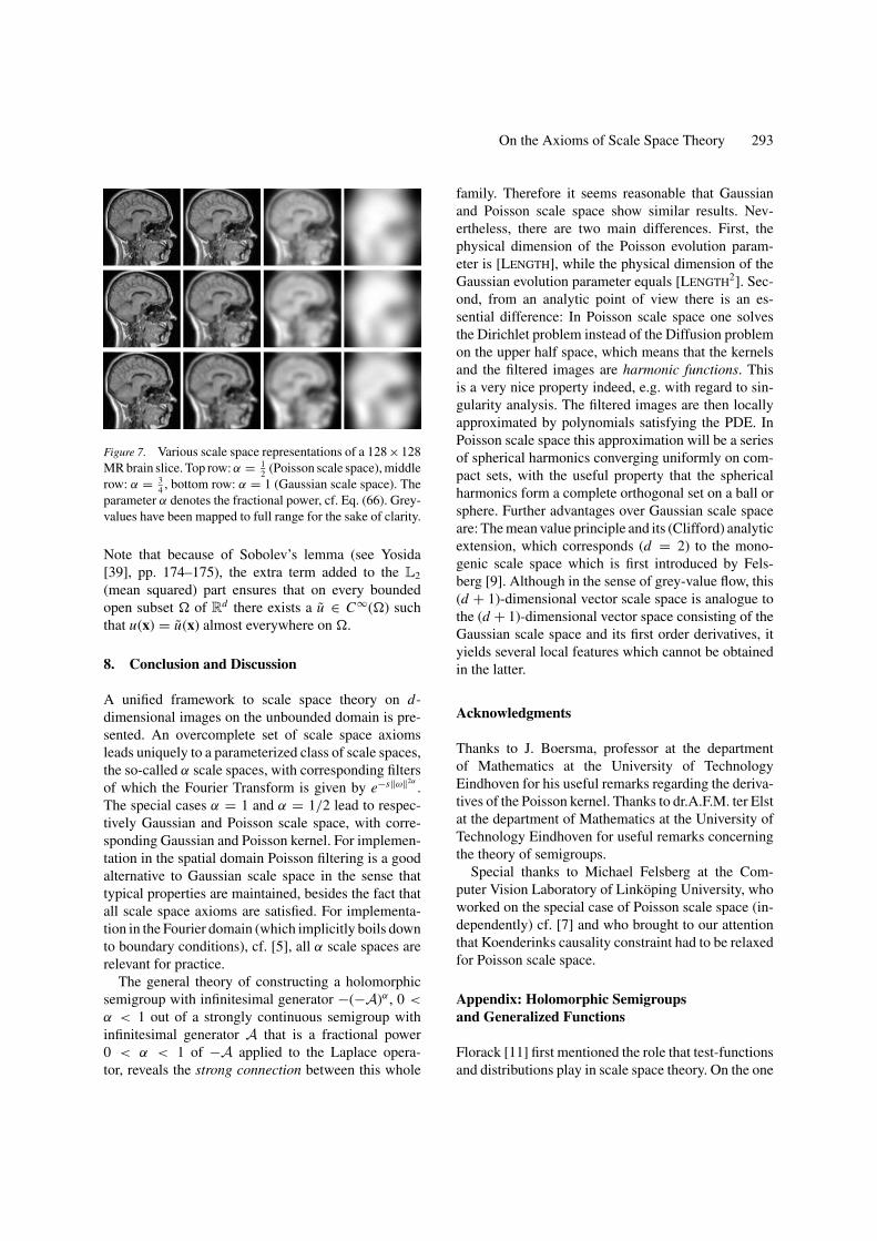
On the Axioms of Scale Space Theory 293
Figure 7. Various scale space representations of a 128×128MR brain slice. Top row: α = 1
2 (Poisson scale space), middlerow: α = 3
4 , bottom row: α = 1 (Gaussian scale space). Theparameter α denotes the fractional power, cf. Eq. (66). Grey-values have been mapped to full range for the sake of clarity.
Note that because of Sobolev’s lemma (see Yosida[39], pp. 174–175), the extra term added to the L2
(mean squared) part ensures that on every boundedopen subset � of Rd there exists a u ∈ C∞(�) suchthat u(x) = u(x) almost everywhere on �.
8. Conclusion and Discussion
A unified framework to scale space theory on d-dimensional images on the unbounded domain is pre-sented. An overcomplete set of scale space axiomsleads uniquely to a parameterized class of scale spaces,the so-called α scale spaces, with corresponding filtersof which the Fourier Transform is given by e−s‖ω‖2α
.The special cases α = 1 and α = 1/2 lead to respec-tively Gaussian and Poisson scale space, with corre-sponding Gaussian and Poisson kernel. For implemen-tation in the spatial domain Poisson filtering is a goodalternative to Gaussian scale space in the sense thattypical properties are maintained, besides the fact thatall scale space axioms are satisfied. For implementa-tion in the Fourier domain (which implicitly boils downto boundary conditions), cf. [5], all α scale spaces arerelevant for practice.
The general theory of constructing a holomorphicsemigroup with infinitesimal generator −(−A)α , 0 <
α < 1 out of a strongly continuous semigroup withinfinitesimal generator A that is a fractional power0 < α < 1 of −A applied to the Laplace opera-tor, reveals the strong connection between this whole
family. Therefore it seems reasonable that Gaussianand Poisson scale space show similar results. Nev-ertheless, there are two main differences. First, thephysical dimension of the Poisson evolution param-eter is [LENGTH], while the physical dimension of theGaussian evolution parameter equals [LENGTH2]. Sec-ond, from an analytic point of view there is an es-sential difference: In Poisson scale space one solvesthe Dirichlet problem instead of the Diffusion problemon the upper half space, which means that the kernelsand the filtered images are harmonic functions. Thisis a very nice property indeed, e.g. with regard to sin-gularity analysis. The filtered images are then locallyapproximated by polynomials satisfying the PDE. InPoisson scale space this approximation will be a seriesof spherical harmonics converging uniformly on com-pact sets, with the useful property that the sphericalharmonics form a complete orthogonal set on a ball orsphere. Further advantages over Gaussian scale spaceare: The mean value principle and its (Clifford) analyticextension, which corresponds (d = 2) to the mono-genic scale space which is first introduced by Fels-berg [9]. Although in the sense of grey-value flow, this(d + 1)-dimensional vector scale space is analogue tothe (d + 1)-dimensional vector space consisting of theGaussian scale space and its first order derivatives, ityields several local features which cannot be obtainedin the latter.
Acknowledgments
Thanks to J. Boersma, professor at the departmentof Mathematics at the University of TechnologyEindhoven for his useful remarks regarding the deriva-tives of the Poisson kernel. Thanks to dr.A.F.M. ter Elstat the department of Mathematics at the University ofTechnology Eindhoven for useful remarks concerningthe theory of semigroups.
Special thanks to Michael Felsberg at the Com-puter Vision Laboratory of Linkoping University, whoworked on the special case of Poisson scale space (in-dependently) cf. [7] and who brought to our attentionthat Koenderinks causality constraint had to be relaxedfor Poisson scale space.
Appendix: Holomorphic Semigroupsand Generalized Functions
Florack [11] first mentioned the role that test-functionsand distributions play in scale space theory. On the one

294 Duits et al.
hand there is a state space, i.e. the space of all possiblescalar field configurations and on the other hand thereis a device space consisting of all admissible detectordevices. It seems reasonable, from a physical point ofview to describe a model for the detector device and toprescribe the state space by duality. Since the Gaussiankernels lie in the (Fourier invariant) Schwartz spaceS, one can take it as a device space. As a result thestate space is the set of all tempered distributions S ′.In [17] De Graaf has derived a theory of generalizedfunctions based on holomorphic semi-groups. In thisappendix we will apply little of this theory onto thePoisson semigroup.
In a Hilbert Space X we consider the evolutionequation
du
ds= Au
with A a negative unbounded self-adjoint operator. Ais the infinitesimal generator of a holomorphic semi-group. Solutions u(·) : (0, ∞) → X of this equationare called trajectories. Such a trajectory may or maynot correspond to an “initial condition at s = 0” in X .The set of trajectories is considered as a space of gen-eralized functions. The test function space is defined tobe
SX,A =⋃s>0
esA(X ).
Theorem 11. Let X be a Banach space. Let Q bea strongly continuous, holomorphic semigroup, withinfinitesimal generator A < 0. Then SX,A consists ex-actly of those f ∈ D(A∞) such that
∞∑k=1
sk
k!‖Ak f ‖ < ∞ for a certain s > 0. (79)
Proof: “⊂”: Let x ∈ SX,A ⇒ ∃s>0 ∃xs∈X x = Qs xs .Now since Q is holomorphic, there exists a M > 0 that‖AQs‖ ≤ M s−1, see (23). Consequently,
‖An x‖ = ‖(AQs/n)n xs‖≤ Mn(n/s)n ‖xs‖≤ (eM/s)nn! ‖xs‖
where we have used the elementary inequality nn ≤enn!. With these bounds it is now obvious that∑∞
k=1sk
k! ‖Ak f ‖ < ∞.
“⊃”: Let x ∈ D(A∞), such that (79) is convergent.Choose t > 0 such that
∑∞n=1
sn
n! ‖An x‖ < ∞ for alls ≤ 2t . Since X is a Banach space, we have for s ∈(0, t)
xs =∞∑
k=1
sk
k!(−A)k x exists in X,
(The sequence of partial sums is a Cauchy sequence).By differentiation we have x = Qs xs = esAxs . �
Remark. Elements of D(A∞) that satisfy (79) are of-ten called analytic vectors. If (79) holds for any s > 0then then they are called entire analytic vectors.
Example: The Test Space Corresponding toPoisson Filtering
In this paragraph we will only observe d = 1.The test function space which belongs to the
Dirichlet problem (27) is given by SL2(Rd ),−√−�,
which—as we shall next show—equals a Gelfand-Shilov space, namely
SL2(Rd ),−√−� = S1. (80)
If the reader is not familiar with Gelfand-Shilov spaceshe/she is referred to Gelfand and Shilov [15] (2nd edi-tion, Chap. 4) for a general and profound theory withregard to their spaces. For our purposes we will onlyneed S1, S1, S1,A, S1,A. First we give the definitionsof these spaces and then we give a short overviewof main results with references, about these Gelfand-Shilov spaces and finally we will show (80). Recall thatthe Schwartz space S consists of all φ ∈ C∞(R) suchthat,
supx∈R
|xkφ(q)(x)| ≤ mqk for certain mqk < ∞
with (k, q = 1, 2, . . . ). To obtain Gelfand-Shilovspaces, we have to impose conditions on mqk . Below,a summary of conditions on mqk and correspondingGelfand-Shilov spaces:
• S1: mkq = Cq Akkk , with Cq , A > 0 depending onφ.
• S1: mkq = Cq Bqkk , with Cq , B > 0 depending onφ.
• S1,A: mkq = Cq ¯(A + δ)kkk , with Cq depending onφ and any δ > 0.

On the Axioms of Scale Space Theory 295
• S1,B : mkq = Cq ¯(B + δ)qkk , with Cq depending onφ and any δ > 0.
The following relations hold:
• The test space S1 = {φ ∈ C∞(R) : |φ(q)(x)| ≤Cqe−a|x |1/α }, with a = α
eA1/α depending onφ. The ideabehind this equality is that infξ∈R
kk
|ξ |k = O(e− 1e |ξ |) .
• The test space S1 consists of all functions φ in C∞(R)which can be extended analytically onto a strip {z ∈C : |�(z)| ≤ h(φ)}, which width h(φ) depends on φ.All members of S1 are analytic, since the remainder| hq
q! φ(q)(x + θh)| of a Taylor expansion smaller than
|h|qq! C0 Bqqq .25
• Fourier Transform F maps S1 onto S1 and visaversa.26 Note thatF2 is an isometrical mapping fromS1 (S1) onto itself, since it maps x �→ φ(x) ontox �→ φ(−x).
• The space S1,A consists exactly of those infinitelydifferentiable functions that satisfy
|φ(q)(x)| ≤ Cqδe−(a−δ)|x | δ > 0
• The spaceS1 (S1) is the union of allS1,A (S1,B), A >
0 (B > 0), i.e.
S1 =⋃A>0
S1,A,
S1 =⋃B>0
S1,B .
A sequence {φn} ⊂ S1 converges to zero, if all φn
belong to some S1,A in which they converge to zero.
Note that we assumed functions to be infinitely dif-ferentiable. We will use analytic vectors f . In thesemi-groups, we are interested in (Poisson and Gaus-sian) we have (respectively) D(A∞) = ⋂∞
n=1 Hn =⋂∞n=1 H2n = H∞. This space consists of all functions,
whose generalized derivatives have finite L2-norms. Tothis end we notice that by Sobolevs lemma (Yosida [39]pp. 174–175) states that such functions are indeed al-most everywhere infintely differntiable functions in theusual sense. So, we then arive at a special case of theabove. For instance the space S1 will now consists ofall infinitely differentiable functions f which can beextended analytically on a strip with widht h along thereal axis in the complex plane such that
sup−h<y<h
∫ ∞
−∞| f (x + iy)|2 dx < ∞.
This space equals the space SL2(Rd ),−√−�, since
SL2(Rd ),−√−� = F−1F
(⋃s>0
e−sA(L2(Rd ))
)
= F−1
(⋃s>0
e−s|ω|(L2(Rd ))
)
= F−1
(⋃s>0
S1,s
)= F−1S1 = S1.
Notes
1. Following Pauwels we dismiss separability as a viable basicaxiom, since it is a coordinate dependent notion. It is a straight-forward that any C1, normalised filter which is both separableand isotropic must be a Gaussian, see (69).
2. The usual causality principle must be relaxed, but the main resultremains.
3. Scale space theory can be approached in three ways: as semi-groups, as evolution equations (partial differential equations)and as stochastic processes (probability theory). This arti-cle handles with the first two approaches, but the connec-tion with probability theory will be further examined in futurework.
4. Formally, the Laplace Transform maps the space L2(R+) ontothe Hardy Lebesgue class H2(0), cf. [39] p. 163.
5. To every f ∈ L1(Rd ) corresponds a distribution f . Notethat the definitions of Fourier transform of resp. f and f
coincide (as they should): ˆ( f )(φ) = f (φ) = ∫f φ =∫
f φ = ( f )(φ). Moreover, the same argument is valid iff ∈ L2(Rd ).
6. Using Cauchy Schwarz and the fact that u → f for s ↓ 0 in L2
sense one obtains that E(u) is also continuous in 0.7. In a Hilbert space the Riesz identification identifies the original
space with its dual.8. This coincides for the case α = 1/2 (Poisson semigroup) with
a general result on strongly elliptic forms. See Robinson [32]Proposition 3.6.
9. This boundary condition ensures that the average grey value ismaintained. Analogue to thermic isolation in heat physics.
10. One can show that such a limit always exist.11. For the constant α in part 2. of (23) in the Poisson case, see
proof of Theorem 10.12. Moreover if a function satisfies the mean value principle, then
it must be harmonic!13. Notice that this function cannot be a scale space function.14. f (a) = 1
τn Rn
∫Ba,R
f (x) dx, a ∈ �, R > 0.15. It is shown in Robinson [32] p. 49 that the Hilbert transform is
unbounded as an operator from L∞(R).16. Physically, one could say that the potential field of a positive
charge and that of a mirrored negative charge cancel out alongs = 0.
17. It is sloppy to use �S(x, y) = −δ(x − y) and apply Greenssecond identity on � = R
d × R+, but interesting enough the
result is the same.

296 Duits et al.
18. If restricted to the subspace of analytic signals the Cauchy op-erator is an isometric isomorphism such that the non tangen-tial limit lims↓0 Cg(·, s) = g(·) for all g ∈ H2(∂C+), cf. [16]p. 113.
19. Actually, Sufficiently smooth should be replaced by analyticvectors, see Appendix, but in order to avoid confusion withanalytic function this term is avoided.
20. In general inverse Laplace transformation can be done by usingthe inversion formula
f (λ) = 1
2π i
∫ σ+i∞
σ−i∞eλz[L( f )](z) dz
with σ such that L( f )(z) is analytic on �(z) ≥ σ . So, qs,α is infact the inverse Laplace transform of µ �→ e−sµα
.21. Equation (52) corresponds to the scale invariance axiom,
Axiom 3.22. One might think of using the Campbell-Baker-Hausdorff
formula, since the clifford product commutator is known.23. Formally, we have s > 0 so �n is only defined for s > 0.
Therefore, use Schwarz reflection principle if necessary.24. Substitute (z−2is) for z in the expansion of w(|z|2) with respect
to |z|2 = zz.25. From Stirling’s Formula q! = qq+(1/2)e−q
√2π Eq (Eq → 1)
it follows that h(q) = 1B(φ)e .
26. In general we have F(Sβα ) = F(Sα
β ), so the Fourier invariantspaces are Sα
α . For example the Schwarz-Space, α = ∞.
References
1. L. Alvarez, F. Guichard, P.L. Lions, and J.-M. Morel, “Axiomsand fundamental equations of image processing,” Arch. Rat.Mech. Anal., Vol. 123, pp. 200–257, 1993.
2. V. Balakrishnan, “Fractional powers of closed operators and thesemi-groups generated by them,” Pacific J. Math., Vol. 10, pp.419–437, 1960.
3. A.V. Bukhvalov and W. Arendt, “Integral representation of re-solvent and semigroups,” Pacific J. Math., Vol. 10, pp. 419–437,1960.
4. J. De Graaf, “Evolution equations,” Technical report, TUE,Potugal, March 1996. Course delivered at the Department ofMathematics of the University of Coimbra.
5. R. Duits, M. Felsberg, and L.M.J. Florack, “α Scale Spaces ona Bounded Domain,” Proceedings Scale Space Conference, Isleof Skye, UK, June 2003, pp. 494–510.
6. R. Duits, L.M.J. Florack, J. De Graaf, and B.M. ter Haar Romeny,“On the axioms of scale space theory,” Technical report, TUE,The Netherlands, Eindhoven, Jan. 2002.
7. M. Felsberg, Low-Level Image Processing with the StructureMultivector. PhD thesis, Institute of Computer Science andApplied Mathematics Christian-Albrechts-University of Kiel,2002.
8. M. Felsberg, R. Duits, and L.M.J. Florack, “The monogenic scalespace on a bounded domain and its applications,” ProceedingsScale Space Conference, Isle of Skye, UK, June 2003, pp. 209–224.
9. M. Felsberg and G. Sommer, “Scale adaptive filtering derivedfrom the Laplace equation,” in 23. DAGM Symposium Muster-erkennung, Munchen, B. Radig and S. Florczyk (Eds.), volume2191 of Lecture Notes in Computer Science, Springer: Heidel-berg, 2001, pp. 124–131.
10. M. Felsberg and G. Sommer, “The Poisson scale-space: Aunified approach to phase-based image processing in scale-space,” Journal of Mathematical Imaging and Vision, 2002.submitted.
11. L.M.J. Florack, Image Structure, volume 10 of Computa-tional Imaging and Vision Series. Kluwer Academic Publishers:Dordrecht, The Netherlands, 1997.
12. L.M.J. Florack, A geometric model for cortical magnifica-tion. In Biologically Motivated Computer Vision: Proceed-ings of the First IEEE International Workshop, BMCV 2000(Seoul, Korea, May 2000), S.-W. Lee, H. H. Bulthoff, andT. Poggio (Eds.), volume 1811 of Lecture Notes in Com-puter Science, Springer-Verlag: Berlin, May 2000, pp. 574–583.
13. L.M.J. Florack, R. Maas, and W.J. Niessen, “Pseudo-linearscale-space theory,” International Journal of Computer Vision,Vol. 31, No. 2/3, pp. 247–259, 1999.
14. L.M.J. Florack, A.H. Salden, B.M. ter Haar Romeny, J.J.Koenderink, and M.A. Viergever, “Nonlinear scale-space,” Im-age and Vision Computing, Vol. 13, No. 4, pp. 279–294,1995.
15. Gelfand and Shilov, Generalized Functions. Academic pressInc.: New York, 1968.
16. J.E. Gilbert and M.A.M. Murray, Clifford Algebras and DiracOperators in Harmonic Analysis. Cambridge University Press:Cambridge, 1991.
17. J. de Graaf, “A theory of generalized functions based on holo-morphic semi-groups,” Koninklijke Nederlandse Akademie vanWetenschappen, Department of Mathematics TUE, Series A,Vol. 87, No. 2, pp. 419–437, 1984.
18. C.W. Groetsch, Elements of Applicable Functional Analysis.Marcel Dekker Inc., New York, Basel, 1980.
19. B.M. ter Haar Romeny, L.M.J. Florack, J.J. Koenderink, andM.A. Viergever (Eds.), Scale-Space Theory in Computer Vi-sion: Proceedings of the First International Conference, Scale-Space’97, Utrecht, The Netherlands, vol. 1252 of LectureNotes in Computer Science. Springer-Verlag: Berlin, July1997.
20. E. Hille and R.S. Phillips, Functional Analysis and Semi-Groups.American Mathematical Society, 1957.
21. R.A. Hummel (Ed.), Proc. IEEE Comp. Soc. Conf. ComputerVision and Pattern Recognition, Miami Beach, IEEE, June 22–26, 1986.
22. T. Iijima, “Basic theory of pattern observation,” Papers of Tech-nical Group on Automata and Automatic Control, 1959. (inJapanese).
23. T. Iijima, “Basic theory on normalization of a pattern(in case of typical one-dimensional pattern),” Bulletin ofElectrical Laboratory, Vol. 26, pp. 368–388, 1962. (inJapanese).
24. M. Kerckhove (Ed.), Scale-Space and Morphology in Com-puter Vision: Proceedings of the Third International Conference,Scale-Space 2001, Vancouver, Canada, volume 2106 of Lec-ture Notes in Computer Science. Springer-Verlag: Berlin, July2001.
25. J.J. Koenderink, “The structure of images,” Biological Cyber-netics, Vol. 50, pp. 363–370, 1984.
26. T. Lindeberg, “Scale-space for discrete signals,” IEEE Transac-tions on Pattern Analysis and Machine Intelligence, Vol. 12, No.3, pp. 234–245, 1990.

On the Axioms of Scale Space Theory 297
27. T. Lindeberg, Scale-Space Theory in Computer Vision.The Kluwer International Series in Engineering and Com-puter Science. Kluwer Academic Publishers: Dordrecht, TheNetherlands, 1994.
28. M. Nielsen, P. Johansen, O.F. Olsen, and J. Weickert (Eds.),Scale-Space Theories in Computer Vision: Proceedings ofthe Second International Conference, Scale-Space’99, Corfu,Greece, Vol. 1682 of Lecture Notes in Computer Science.Springer-Verlag, Berlin, Sept. 1999.
29. N. Otsu, Mathematical Studies on Feature Extraction in PatternRecognition. PhD thesis, Electrotechnical Laboratory, Ibaraki,Japan, 1981 (in Japanese).
30. E.J. Pauwels, L.J. Van Gool, P. Fiddelaers, and T. Moons,“An extended class of scale-invariant and recursive scalespace filters,” IEEE Transactions on Pattern Analysisand Machine Intelligence, Vol. 17, No. 7, pp. 691–701,1995.
31. M.H. Protter, Maximum Principles in Differential Equations.Prentice-Hall Inc.: New Jersey, 1967.
32. D.W. Robinson, Elliptic Operators and Lie Groups. ClarendonPress: Oxford, New York, Tokyo, 1991.
33. W. Rudin, Functional Analysis. McGRaw-Hill: New York, 1973.34. K.I. Sato, Levy Processes and Infinitely Divisible Dis-
tributions. Cambridge University Press: Cambridge,1999.
35. J. Sporring, M. Nielsen, L. Florack, and P. Johansen, GaussianScale-Space Theory. KAP: Dordrecht, The Netherlands,1997.
36. J. Sporring, M. Nielsen, L.M.J. Florack, and P. Johansen(Eds.), Gaussian Scale-Space Theory, Volume 8 of Computa-tional Imaging and Vision Series. Kluwer Academic Publishers:Dordrecht, The Netherlands, 1997.
37. J.A. Weickert, Anisotropic Diffusion in Image Processing. ECMISeries. Teubner, Stuttgart, Jan. 1998.
38. J.A. Weickert, S. Ishikawa, and A. Imiya, “On the historyof Gaussian scale-space axiomatics,” in Sporring et al. [36],Chap. 4, pp. 45–59, 1997.
39. K. Yosida, Functional Analysis. Springer Verlag: Berlin,Heidelberg, New York, 1980.
Remco Duits received his M.Sc. degree in Mathematics in 2001from Eindhoven University of Technology, The Netherlands. Cur-rently he is a PhD student at the Department of Biomedical En-gineering on Eindhoven University of Technology on the subjectof multi-scale perceptual grouping. His interest subtends functionalanalysis, group theory, partial differential equations, multiscale rep-resentations and their applications to biomedical imaging and vision,perceptual grouping.
Luc Florack received his M.Sc. degree in theoretical physics in 1989,and his Ph.D. degree in 1993 with a thesis on image structure, bothfrom Utrecht University, The Netherlands. During the period 1994–1995 he was an ERCIM/HCM research fellow at INRIA Sophia-Antipolis, France, and INESC Aveiro, Portugal. In 1996 he was anassistant research professor at DIKU, Copenhagen, Denmark, on agrant from the Danish Research Council. From 1997 until 2001 hehas been working as an assistant professor at Utrecht University,first at the Department of Computer Science, and subsequently at theDepartment of Mathematics. Currently he is employed as an associateprofessor with Eindhoven University of Technology, Department ofBiomedical Engineering. His interest subtends all structural aspectsof signals, images and movies, notably multiscale representations,and their applications to imaging and vision.
Jan de Graaf is Professor of Mathematics at the Eindhoven Univer-sity of Technology in The Netherlands, Chair: Applied Analysis. Hehas been educated as an Electrical Engineer, as a Physicist and as aMathematician.
Current research topics: (strongly non-linear) evolution equationsin Banach spaces applies to free boundary value problems in fluiddynamics; fractional evolution equations; (hyper-) complex methodsto fluid mechanics, to operator theory and to measurement theory inquantum mechanics.
Author of the books: S.J.L. Van Eijnhoven, J. de Graaf. A math-ematical Introduction to Dirac’s Formalism North-Holland Math.Library, Amsterdam (1986). S.J.L. Van Eijnhoven, J. de Graaf. Tra-jectory Spaces, Generalized Functions and Unbounded Operators(L.N.M., 1162). Springer Berlin (1985).
Supervisor of (recently defended) Ph.D. Theses on: Movingboundary problems in relation with equations of Loewner-Kufarevtype; Parabolic evolution equations for quasi stationary free boundaryproblems in capillary fluid dynamics; Fractional Evolution equationsin Banach spaces; Perturbation and operator methods for solvingStokes flow and heat flow problems; Reduced heat kernels on homo-geneous spaces; Positive operator-valued measures and phase-spacerepresentations.

298 Duits et al.
Bart M. ter Haar Romeny is full professor in Biomedical ImageAnalysis at the Department of Biomedical Engineering at EindhovenUniversity of Technology since 2001. He received a M.Sc. in Applied
Physics from Delft University of Technology in 1978, and a Ph.D. onneuromuscular nonlinearities from Utrecht University in 1983. Af-ter being the principal physicist of the Utrecht University HospitalRadiology Department he joined in 1989 the department of MedicalImaging at Utrecht University as associate professor. His interestsare mathematical aspects of visual perception, in particular linearand non-linear scale-space theory, computer vision applications, andall aspects of medical imaging. He is author of numerous papers andbook chapters on these issues, edited a book on non-linear diffusiontheory and is author of an interactive tutorial book on scale-spacetheory in Computer Vision. He initiated a number of internationalcollaborations on those subjects. He is an active teacher in (inter-)national courses, a senior member of IEEE, and IEEE Chapter Tu-torial Speaker. He is chairman of the Dutch Biophysical Society.