Embed Size (px)
Citation preview
Computer Aided Geometric Design 20 (2003) 319–341www.elsevier.com/locate/cagd
On the angular defect of triangulations andthe pointwise approximation of curvatures ✩
V. Borrelli a, F. Cazals b,∗, J.-M. Morvan a,b
a Institut Girard Desargues, Univ. Lyon I, Mathematiques, 43 Boulevard du 11 Novembre 1918, F-69622 Villeurbanne, Franceb INRIA Sophia-Antipolis, 2004 route des Lucioles, F-06902 Sophia-Antipolis, France
Received 17 October 2002; received in revised form 16 April 2003; accepted 24 April 2003
Abstract
Let S be a smooth surface of E3, p a point on S, km, kM , kG and kH the maximum, minimum, Gauss andmean curvatures of S at p. Consider a set {pippi+1}i=1,...,n of n Euclidean triangles forming a piecewise linearapproximation of S around p—with pn+1 = p1. For each triangle, let γi be the angle � pippi+1, and let the angulardefect at p be 2π − ∑
i γi . This paper establishes, when the distances ‖ppi‖ go to zero, that the angular defect isasymptotically equivalent to a homogeneous polynomial of degree two in the principal curvatures.
For regular meshes, we provide closed forms expressions for the three coefficients of this polynomial. We showthat vertices of valence four and six are the only ones where kG can be inferred from the angular defect. Atother vertices, we show that the principal curvatures can be derived from the angular defects of two independenttriangulations. For irregular meshes, we show that the angular defect weighted by the so-called module of the meshestimates kG within an error bound depending upon km and kM .
Meshes are ubiquitous in Computer Graphics and Computer Aided Design, and a significant number of papersadvocate the use of normalized angular defects to estimate the Gauss curvature of smooth surfaces. We showthat the statements made in these papers are erroneous in general, although they may be true pointwise for veryspecific meshes. A direct consequence is that normalized angular defects should be used to estimate the Gausscurvature for these cases only where the geometry of the meshes processed is precisely controlled. On a moregeneral perspective, we believe this contributions is one step forward the intelligence of the geometry of meshes,whence one step forward more robust algorithms.© 2003 Elsevier B.V. All rights reserved.
Keywords: Smooth surfaces; Meshes; Curvatures; Approximations; Differential geometry
✩ Partially supported by the Effective Computational Geometry for Curves and Surfaces European project, Project No IST-2000-26473.
* Corresponding author.E-mail addresses: [email protected] (V. Borrelli), [email protected] (F. Cazals),
[email protected] (J.-M. Morvan).
0167-8396/$ – see front matter © 2003 Elsevier B.V. All rights reserved.doi:10.1016/S0167-8396(03)00077-3

320 V. Borrelli et al. / Computer Aided Geometric Design 20 (2003) 319–341
1. Introduction
1.1. Smooth and triangulated surfaces
Meshes are ubiquitous in modern computer-related geometry. Meshes are easily obtained fromphysical objects through scanning and reconstruction. Meshes are commonly displayed by graphicalhardware. Meshes are intuitive to deal with. They provide hierarchical representations that can be usedfor approximate representations. Meshes can be refined to smooth surfaces through subdivision.
In this context, and especially since meshes can be made dense enough so as to “look like” smoothsurfaces, it is tempting to define a differential geometry of meshes which mimics that of smooth surfaces.
Example quantities well defined smooth surfaces that also look appealing for meshes are the surfacearea, the normal vector field, the curvatures, geodesics, the focal sets, the ridges, the medial axis, etc.
Interestingly, recent research in applied domains provides, for each of the notions just enumerated,several estimates adapted from classical differential geometry to the setting of piecewise linear surfaces.Several definitions of normals, principal directions and curvatures over a mesh can be found in (Taubin,1995; Meyer et al., 2002). Ridges of polyhedral surfaces as well as cuspidal edges of the focal setsare computed in (Watanabe and Belyaev, 2001). Geodesics and discrete versions of the Gauss–Bonnettheorem are considered in (Polthier and Schmies, 1998). But none of these contributions address thequestion of the accuracy of these estimates or that of their convergence when the mesh is refined.
As opposed to these approaches, the literature provides a few examples of a priori analysis. Given adiscrete set—a point cloud or a mesh—which is assumed to sample a surface in a certain way, differentialoperators are derived together with theoretical guarantees about the discrepancy between the discreteestimates and the true value on the underlying smooth surface.
In (Amenta and Bern, 1999) it is shown that the normal to a smooth surface sampled according to a cri-terion involving the skeleton can be estimated accurately from the Voronoi diagram of the sample points.The surface area of a mesh and its normal vector field versus those of a smooth surface are considered in(Morvan and Thibert, 2001). More closely related to the question we address is (Meek and Walton, 2000),which provides some error bounds for estimates of the normal and the Gauss curvature of a sampledsurface. In particular, Meek and Walton observe on a counterexample that the angular defect does not es-timate the Gauss curvature, but no analysis is carried out. The missing analysis is presented in this paper.
1.2. Smooth surfaces, polyhedra, Gauss curvature and angular defect
In this section, we hi-light striking parallels between the Gauss curvature of polyhedra and smoothsurfaces of E3. More precisely, we recall:
(1) the definition of the Gauss curvature for smooth surfaces and polyhedra, as well as the Gauss–Bonnettheorem in both cases.
(2) how the Gauss curvature of a smooth surface can be recovered from the angular defect of geodesictriangles.
1.2.1. Gauss curvature and the Gauss–Bonnet theorem for surfaces and polyhedraThe Gauss curvature of an (abstract) oriented smooth Riemannian surface M is a smooth function
kG on M defined by using the metric tensor. It is well known that the Gauss curvature of a domain is

V. Borrelli et al. / Computer Aided Geometric Design 20 (2003) 319–341 321
identically equal to zero if and only if it is locally isometric to a portion of plane. One can associate tokG a curvature measure KG on M by integration over any domain U of M :
KG(U) =∫U
kG da,
where da denotes the area form of M . Suppose now that M is isometrically embedded in E3. One wayto evaluate its Gauss curvature at a point p is to make the product of the two principal curvatures of M
at p (this is nothing but theorema egregium of Gauss). An equivalent way it to use the Gauss map ofthe embedding and to calculate the limit A′/A, where A is the surface area of a region around p, A′ thesigned area of the image of A on S2 by the Gauss map, the limit being taken (roughly speaking) as theregion A around p becomes smaller and smaller (Spivak, 1999, Vol. 2, Chapter III).
Consider now an abstract Riemannian polyhedron P . Any point of P which is not a vertex has aneighborhood isometric to a plane, and one can define its Gauss curvature to be 0, by analogy with thesmooth case. Moreover, if p is a vertex of P , one can assign to p the angular defect αp = 2π − ∑
i γi
at p, where the γis stand for the angles at p of the facets incident to p. We call this angular defect theGauss curvature kG(p) of the vertex p (Reshetnyak, 1993, Section 5). Remark that it is now possible todefine a curvature measure on P , as a measure concentrated on the vertices of P , by setting over anydomain U of P
KG(U) =∑
p vertex in U
α(p).
If P is isometrically embedded in E3, then this angular defect is exactly the signed area of the image onS2 by the Gauss map of any arbitrarily small neighborhood of p, which is a property analogous to thesmooth case.
An important relationship relating the Gauss curvature to topological properties is the Gauss–Bonnettheorem. Consider a closed orientable surface S and a closed polyhedron P , the latter with verticesp1, . . . , pn. Let χ(S) and χ(P ) stand for their Euler characteristic—that is V − E + F in the usualjargon. The global Gauss–Bonnet theorem respectively states for S and P that—for the polyhedral case,see (Banchoff, 1967):
2πχ(S) =∫ ∫
S
kG dσ, (1)
2πχ(P ) =∑
i=1,...,n
kG(pi). (2)
These remarkable results actually state that if the topology is fixed—i.e., the genus of the surface or thepolyhedron is given, the curvature distributes itself on S or P so as to comply with that topology. Noticethat local versions of both theorems exist. (For the geodesic curvature involved in the local Gauss–Bonnettheorem, see (Reshetnyak, 1993; Polthier and Schmies, 1998).)
Remark that in this context, the Gauss curvature of a point of a polyhedron is dimensionless, whilethat of a surface is homogeneous to the inverse of a surface area. The topological invariant 2πχ isdimensionless, which is coherent with Eqs. (1) and (2).

322 V. Borrelli et al. / Computer Aided Geometric Design 20 (2003) 319–341
Fig. 1. Flattening a geodesic triangle yields an estimate for the Gauss curvature.
1.2.2. Gauss curvature and geodesic trianglesAn important property of geodesic triangles also which involves the Gauss curvature is the following—
see (Cheeger et al., 1984; Lafontaine, 1986).Let τi be a geodesic triangle on S, p, pi and pi+1 its vertices, lp, li , li+1 the lengths of the geodesic
arcs opposite to the vertices, and l = sup{li, li+1}. Let Ti be the Euclidean triangle whose edges have thesame lengths as those of τi . We call Ti a Euclidean geodesic triangle since it is a Euclidean triangle,but its edges’ lengths are geodesic distances. Finally, let βi be the angle of τi at p, and αi be the angle� pippi+1 of Ti . See Fig. 1 for an illustration. The angles βi and αi differ by a term involving the Gausscurvature kG at p. More precisely, we have
Proposition 1. The angles βi and αi associated to a Euclidean geodesic triangle τi satisfyβi = αi + 1
6 sinαikGli li+1 + o(l2). (3)
Consider now a geodesic triangulation around p, that is a set of n geodesic triangles having p ascommon vertex and forming a topological disk around p. By looking at the tangents to the geodesicsfrom p to the pis, we have
∑i βi = 2π . Summing Eq. (3) for the n geodesic triangles immediately
yields the following
Theorem 1. Let T be a geodesic triangulation of a smooth surface M of E3. Let p be a vertex of T , andlet A(p) be the sum of the areas of the triangles Ti associated to the Euclidean geodesic triangles τis.Then
2π −∑
i
αi = A(p)
3kG + o(l2).
This result is of little help from a practical standpoint since the knowledge of geodesics is required.The question addressed in this paper is actually to study the quantity estimated by the angular defectwhen one replaces the geodesics by the Euclidean line-segments ppi .
1.3. Question addressed in this paper
Let S be a surface of E3, and let p be a point of S. Also suppose that we are given a set {pippi+1}i=1,...,n
of n Euclidean triangles forming a piecewise linear approximation of S around p. We shall refer to these

V. Borrelli et al. / Computer Aided Geometric Design 20 (2003) 319–341 323
triangles as the mesh, and to the pis as the one-ring neighbors of p. For each triangle, let γi be the angle� pippi+1, and let the angular defect at p be 2π − ∑
i γi . Also, for a one-ring neighbor pi , let ηi standfor the Euclidean distance between p and pi .
The question we address in this paper is:
How precisely can one estimate the curvatures at a point p of a smooth surface using the angulardefect of the triangles surrounding p?
Before presenting the contributions, several comments are in order.
Dimensionality. In order for the previous question to make sense, we shall pay a special attention tothe dimensionality of the quantities involved. As already pointed out, the Gauss curvature of a smoothsurface is homogeneous to the inverse of a surface area while that of a polyhedron is dimensionless. Toestimate the curvatures of a smooth surface from a polyhedron, we will therefore have to normalize bylengths (for the principal curvatures) or surface areas (Gauss curvature).
Smooth surfaces and asymptotic estimates. Estimating the curvatures of a smooth surface S from asingle mesh is obviously an hopeless target. The folds of S may indeed occur at a resolution much lowerthan that of the triangulation, so that the mesh may fall short from providing accurate information onthe point-wise curvatures. The problem becomes more tractable if one assumes S belongs to a restrictedclass of surfaces—e.g., with Lipchitz like conditions on the variation of the normal—or assumes that asequence of meshes with edges’ lengths going to zero is available. We shall in the paper follow this latterperspective and derive asymptotic results.
Soundness of the angular defect for the Gauss curvature of smooth surfaces. Since the angular defectover geodesic triangles provides an estimate of kG, it is tempting to believe that when the edges lengths‖ppi‖ go to zero, one can safely replace the geodesic arcs from p to the pis on S by the Euclideansegments ppis. We shall see it is not so.
1.4. Contributions
This paper establishes, when the distances ‖ppi‖ go to zero, that the angular defect is asymptoticallyequivalent to a homogeneous polynomial of degree two in the principal curvatures. To state the results
Fig. 2. Can the curvatures of a smooth surface be estimated from the angular defect of a triangulation?

324 V. Borrelli et al. / Computer Aided Geometric Design 20 (2003) 319–341
more precisely, one need to distinguish between regular and irregular meshes. By regular mesh, we referto a mesh such that the pis lie in normal sections two consecutive of which form an angle of 2π/n, withthe additional constraint that ‖ppi‖ is a constant. A mesh which is not regular is called irregular.
Regular meshes. We provide the closed form expression of the afore-mentioned polynomial as a functionof the principal curvatures and 2π/n. In particular, we show that n = 4 is the only value of n such that2π − ∑
i γi depends upon the principal directions, and that n = 6 is the only value such that 2π − ∑i γi
provides an exact estimate for kG. A corollary of these results is that the principal curvatures—whencekG and kH —can be computed from the angular defects of any two triangulations whose valences are notfour.
Irregular meshes. We show that the angular defect weighted by the so-called module of the meshestimates kG within an error bound depending upon km and kM .
Practical relevance of our results. From a practical standpoint, normalized angular defects areadvocated as an estimator for the Gauss curvature in a significant number of papers—see, e.g., (Calladine,1986; Meyer et al., 2002; Cskny and Wallace, 2000; Dyn et al., 2001). We show that the statements madein these papers are erroneous in general, although they may be true pointwise for very specific meshes.A direct consequence is that normalized angular defects should be used to estimate the Gauss curvaturefor these cases only where the geometry of the meshes processed is precisely controlled.
Finally, it should be emphasized that along the derivation of these results, we prove severalapproximation lemmas for curves and surfaces. These results may find applications in surface meshing,surface subdivision, feature extraction, . . . .
1.5. Paper overview
The paper is organized as follows. Section 2 provides the notations used throughout the paper. InSection 3 we present approximation results for the curvature of plane curves. These results are used inSection 4 to derive a formula on Euclidean triangles providing a piecewise linear approximation of asmooth surface. Using restricted hypothesis on the geometry of these triangles, we show in Section 5that the angular defect does not provide, in general, an estimate for kG. In Section 6, the hypothesisof Section 5 are alleviated and a general result about the accuracy of the angular defect is proved.Illustrations of the main theorems are provided in Section 7.
2. Notations
Consider a point p of a smooth surface together with n Euclidean triangles {pippi+1}i=1,...,n—withpn+1 = p1—forming a piecewise linear approximation of S around p. The following notations are usedthroughout the paper—see Fig. 3:
Normal sections; Πi , ϕi . Consider the plane Πi containing the normal n, p and pi . We assume Πi isdefined by its angle ϕi with respect to some coordinate system in the tangent plane—for example,the one associated with the principal directions.

V. Borrelli et al. / Computer Aided Geometric Design 20 (2003) 319–341 325
Fig. 3. Notations. Fig. 4. pi in spherical coordinates.
Distance to one-ring neighbor; ηi . The Euclidean distance from p to its ith neighbor pi is denoted ηi .Angle between normal sections; βi . The angle between two consecutive normal sections Πi and Πi+1
is denoted βi , that is βi = ϕi+1 − ϕi . Put differently, βi measures, in the tangent plane, the anglebetween the tangents to the plane curves S ∩ Πi and S ∩ Πi+1.
Polyhedral angle; γi . Consider the Euclidean triangle ppipi + 1. The angle at p, i.e., � pippi+1 isdenoted γi . (Notice that the angle γi is different from the angle αi of Proposition 1.)
Directional curvatures; λi . We let λi stand for the curvature of the plane curve S ∩ Πi . Notice that ifΠi contains a principal direction, λi reduces to the corresponding principal curvature kM or km.
3. Plane curves
In this section, we provide an estimate for the curvature of a plane curve from the angular defect of aninscribed polygon.
3.1. A lemma on plane curves
Let C be a C∞ smooth regular curve. Let p0 be a point of C. It is well known that C can locally berepresented by the graph (x, f (x)) of a smooth function f , such that p0 = (0,0) (i.e., f (0) = 0), andsuch that the tangent to C at p0 is aligned with the x-axis (i.e., f ′(0) = 0). Let k be the curvature of C atthe origin (i.e., k = f ′′(0)), and let ν = f ′′′(0). Near the origin we have
f (x) = kx2
2+ νx3
6+ o(x3). (4)
Let us now use polar coordinates: x = η cos θ and y = η sin θ . In order to approximate the curvatureof C at p0, we shall need an expression of θ as a function of η. Obtaining such an expression involvesthe implicit function theorem, and the reader is referred to Appendix A for the proof of the following
Lemma 1. Let f (x) be a C∞ smooth regular function with k = f ′′(0) and ν = f ′′′(0). For a pointp = (η cos θ, η sin θ) on the graph of f near the origin, one has:
θ = kη
2+ νη2
6+ o(η2) if x � 0, (5)
θ = kη
2− νη2
6+ o(η2) if x � 0. (6)

326 V. Borrelli et al. / Computer Aided Geometric Design 20 (2003) 319–341
Fig. 5. Smooth curve and inscribed polygon.
3.2. Approximating the curvature of a plane curve
The previous lemma can be used to estimate the curvature of a curve from the angular defect αi of aninscribed polygon. See Fig. 5 for the notations.
Theorem 2. Let pi−1, pi and pi+1 be three points as indicated on Fig. 5, with ηi−1 (ηi+1) the distancefrom pi to pi−1 (pi+1). Also let ηi = (ηi−1 + ηi+1)/2. The angular defect αi at pi and the curvature k
satisfy:
• if ηi−1 = ηi+1 = η:π − αi
η= k + o(η), (7)
• if ηi−1 �= ηi+1:π − αi
ηi
= k + o(1). (8)
Proof. Since the proofs of the two statements are similar, we focus just on the first one.Eqs. (5) and (6) applied to pi+1 and pi−1 yield θi−1 + θi+1 = kη + o(η2). But we also have
θi−1 + θi+1 = π − αi , whence the result. �Interestingly, the speed of convergence is faster when the two neighbors are located at the same
distance from pi .
Remark. The previous theorem can be extended to space curves.
4. A lemma on normal sections and Euclidean triangles
This section is devoted to a general result involving Euclidean triangles and smooth surfaces. Thisresult is the cornerstone of the next two sections.

V. Borrelli et al. / Computer Aided Geometric Design 20 (2003) 319–341 327
Using the notations of Section 2, we aim at finding a dependence relationship between βi , γi , ηi andηi+1. More precisely, we shall consider that the normal sections Πis are fixed—which determines theϕis, βis and λis—and study the dependence between γi , ηi and ηi+1.
Lemma 2. With the above notations, let η = max(ηi, ηi+1). Define the following sum and productfunctions
s(ηi, ηi+1) = λ2i η
2i + λ2
i+1η2i+1
8, p(ηi, ηi+1) = λiλi+1ηiηi+1
4.
The βi , γi , ηi and ηi+1 quantities satisfy
βi = γi + p(ηi, ηi+1)
sinγi
− s(ηi, ηi+1) cot γi + o(η2) (9)
and
βi = γi + p(ηi, ηi+1)
sinβi
− s(ηi, ηi+1) cotβi + o(η2). (10)
Proof. The proofs of the two claims following the same guideline, we just prove the second one. Assumepoint p is at the origin. Let us write the coordinates of pi in spherical form with the conventions ofFig. 4—that is ϕ measures an angle in the tangent plane of S at p. If Xt stands for the transpose of X,the coordinates of pi are pi = (ηi cos θi cosϕi, ηi cos θi sinϕi, ηi sin θi)
t , and similarly for pi+1.Since βi = ϕi+1 − ϕi , expressing the dot product ppi · ppi+1 = ηiηi+1 cosγi in spherical coordinates
yields
cosγi = cosβi cos θi cos θi+1 + sin θi sin θi+1. (11)
Since the curve Πi ∩ S is a plane curve, using Eq. (5) which expresses θ as a function of η, we have
cos θi = 1 − λ2i η
2i
8+ o(η2
i ), sin θi = λiηi
2+ o(ηi).
Plugging these values into Eq. (11) yields
cosγi = (1 − s(ηi, ηi+1)
)cosβi + p(ηi, ηi+1) + o(η2).
To turn the previous expression into a relationship between γi and βi , we use the Taylor formula of orderone to f (x) = arccos(x) together with a = cosβi and b = cosγi :
γi = βi + −1sinβi
(−s(ηi , ηi+1) cosβi + p(ηi, ηi+1) + o(η2)) + o(η2).
Re-arranging the terms completes the proof. �
5. Surfaces and regular polygons
5.1. Main result and implications
Using the lemma proved in the previous section, we are now ready to analyze the angular defect forregular meshes. We shall need the following definitions.

328 V. Borrelli et al. / Computer Aided Geometric Design 20 (2003) 319–341
Fig. 6. Regular triangulation around p: tangent plane seen from above.
Definition 1. Let p be a point of a smooth surface S and let pi, i = 1, . . . , n be its one ring neighbors.Point p is called a regular vertex if (i) the pis lie in normal sections two consecutive of which form anangle of θ(n) = 2π/n, (ii) the ηis all take the same value η.
Definition 2. Consider the directions of maximum and minimum curvatures of S at p. Assume thesedirections are associated two vectors vM and vm such that vM ∧ vn = n—with n be the normal of S at p.The offset angle a is defined as the angle in [0,2π [ between the vectors vM and pπ(p1) with π(p1) theprojection of p1 in the tangent plane.
Let us now get back to the notations of Section 2 at a regular vertex. Angle a is the angle from vMto the normal section of the first normal section. For a regular vertex, the βis are constant and equal toθ(n), so that ϕi = a + (i − 1)θ(n). Under these hypothesis, we provide a closed form expression for theangular defect. The reader is referred to Appendix B for the proof of the following theorem.
Theorem 3. Consider a regular vertex of valence n. The following holds:
(1) There exists two functions A(a,n) and B(a,n) such that
2π −n∑
i=1
γi = [A(a,n)kG + B(a,n)
(k2M + k2
m
)]η2 + o(η2). (12)
(2) The only value of n such that the functions A(a,n) and B(a,n) depend upon a is n = 4, and then
2π −n∑
i=1
γi = [(1 − 2cos2 a sin2 a)kG + cos2 a sin2 a
(k2M + k2
m
)]η2 + o(η2). (13)
(3) If n �= 4:
2π −n∑
i=1
γi = n
16 sin 2π/n
[(2 − cos
4π
n− cos
2π
n
)kG
+(
1 + 12
cos4π
n− 3
2cos
2π
n
)(k2M + k2
m
)]η2 + o(η2). (14)

V. Borrelli et al. / Computer Aided Geometric Design 20 (2003) 319–341 329
Fig. 7. The coefficients A(a,4), B(a,4) and A(a,4) + B(a,4)—respectively (solid curve, top), (solid curve, bottom), (dottedcurve).
Fig. 8. The coefficients A(a,n), B(a,n) and A(a,n) + B(a,n)—respectively (solid curve, top), (solid curve, bottom), (dottedcurve).
In particular, the only value of n such that B(a,n) = 0 is n = 6, and then A(a,6) = √3/2, that is
2π −∑
i
γi =√
32
kGη2 + o(η2). (15)
The graphs of the functions A(a,4) and B(a,4), as well as A(a,n) and B(a,n) for n �= 4 are presentedon Figs. 7 and 8. For the angular defect to provide an estimate for kG, a sufficient condition is to havea regular triangulation of valence n = 4 with the one-ring neighbors are aligned with the principaldirections. Another sufficient condition is to have a regular valence six triangulation. Therefore, theangular defect is expected to provide good results for triangulations where valence six vertices are
330 V. Borrelli et al. / Computer Aided Geometric Design 20 (2003) 319–341
prominent. Example such triangulations are those generated by subdivision processes. Apart from thetwo favorable configurations just mentioned, several other configurations are of course possible. From apractical standpoint, these results show that normalized angular defects should be used to estimate theGauss curvature for these cases only where the geometry of the meshes processed is precisely controlled.
The valence six almost everywhere observation is also related to the following question. In Section 1.2we recalled the Gauss–Bonnet theorem for a polyhedra P and a compact orientable surface S. AssumeP and S are homeomorphic. An interesting issue is the global convergence of the sum of the angulardefects over P when P is refined so as to converge to S. The fact that valence six vertices are expectedalmost everywhere is certainly related to the answer. Fully resolving this issue is a geometric measuretheory related question.
At last, the previous theorem fully explains the observation made in (Meek and Walton, 2000), basedon a counter-example, that the angular defect does not estimate the Gauss curvature.
5.2. Corollaries
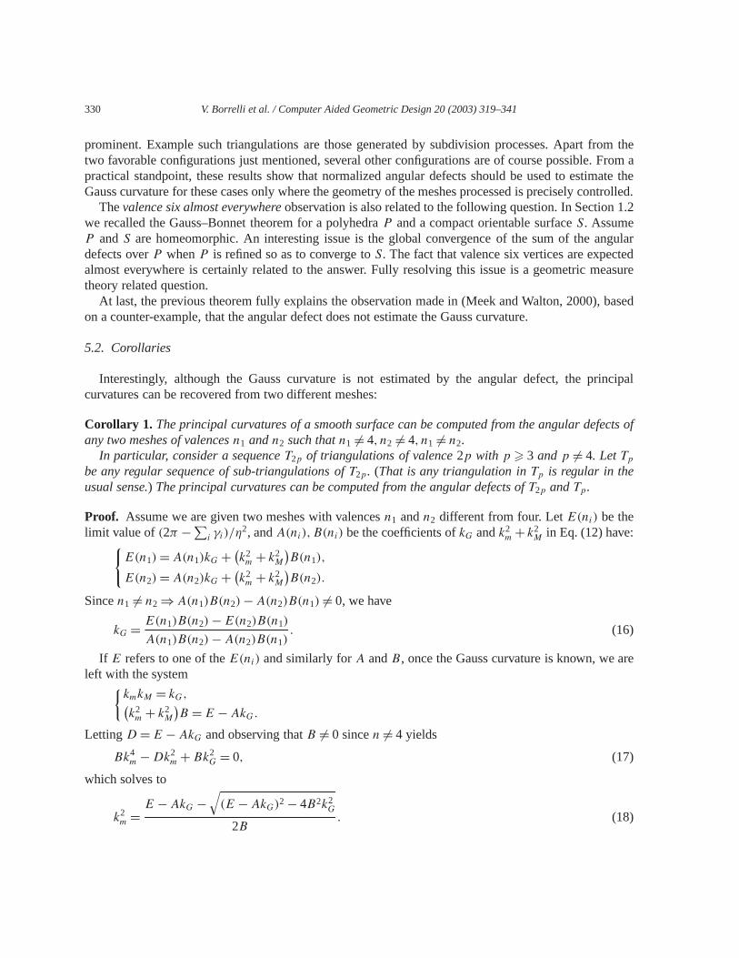
Interestingly, although the Gauss curvature is not estimated by the angular defect, the principalcurvatures can be recovered from two different meshes:
Corollary 1. The principal curvatures of a smooth surface can be computed from the angular defects ofany two meshes of valences n1 and n2 such that n1 �= 4, n2 �= 4, n1 �= n2.
In particular, consider a sequence T2p of triangulations of valence 2p with p � 3 and p �= 4. Let Tp
be any regular sequence of sub-triangulations of T2p . (That is any triangulation in Tp is regular in theusual sense.) The principal curvatures can be computed from the angular defects of T2p and Tp .
Proof. Assume we are given two meshes with valences n1 and n2 different from four. Let E(ni) be thelimit value of (2π −∑
i γi)/η2, and A(ni),B(ni) be the coefficients of kG and k2
m + k2M in Eq. (12) have:{
E(n1) = A(n1)kG + (k2m + k2
M
)B(n1),
E(n2) = A(n2)kG + (k2m + k2
M
)B(n2).
Since n1 �= n2 ⇒ A(n1)B(n2) − A(n2)B(n1) �= 0, we have
kG = E(n1)B(n2) − E(n2)B(n1)
A(n1)B(n2) − A(n2)B(n1). (16)
If E refers to one of the E(ni) and similarly for A and B , once the Gauss curvature is known, we areleft with the system{
kmkM = kG,(k2m + k2
M
)B = E − AkG.
Letting D = E − AkG and observing that B �= 0 since n �= 4 yields
Bk4m − Dk2
m + Bk2G = 0, (17)
which solves to
k2m =
E − AkG −√
(E − AkG)2 − 4B2k2G
2B. (18)

V. Borrelli et al. / Computer Aided Geometric Design 20 (2003) 319–341 331
Notice that the sign of the square root chosen in the previous expression does not matter since the twosolutions corresponding to ±√ are actually conjugated with respect to kmkM = kG, that is
k2M = k2
G
k2m
=E − AkG +
√(E − AkG)2 − 4B2k2
G
2B. (19)
Once k2m and k2
M have been computed, km and kM are determined observing that the product of theirsigns is the sign of kG, and that km � kM . Once km and kM are known, the mean curvature kH iskH = (km + kM)/2.
For the second part, just apply the first part to the two regular sequences of triangulations T2p andTp . �
In the same spirit, we also have:
Corollary 2. Umbilics can be detected from the two angular defects without computing the principalcurvatures.
Proof. At an umbilic point, we have km = kM . Using the notations of the previous proof, it is easilychecked that (E − AkG)2 − 4B2k2
G = 0 and sign(kG) � 0. �Since two meshes are enough to infer the principal curvatures, it is tempting to infer the position
of the principal directions using the valence four mesh and Eq. (13). This equation yields the value ofcos2 a sin2 a, from which one is unable to distinguish between a and 2π − a.
Remark. It is important to notice that Corollary 1 compares the Gauss curvature and the squares of theprincipal curvatures of S against the angular defect normalized by η2—see Section 1.2 for a discussionof the dimensionality issues.
6. Surfaces: the general case
This section generalizes the analysis carried out in the previous section. We relax the hypothesis onthe edges’ lengths ηis as well as on the angles ϕis, and provide an expression of the angular defect as aTaylor expansion in the edges’ lengths.
6.1. Angular defect and kG
We shall need the following definition:
Definition 3. Consider the one-ring neighbors of p. For the sake of conciseness, let ci = cosϕi ,si = sinϕi , and define the following quantities:
Ai = 14 sinγi
[ηiηi+1
(c2i s
2i+1 + s2
i c2i+1
) − cosγi
2(η2
i
(2c2
i s2i
) + η2i+1
(2c2
i+1s2i+1
))], (20)
332 V. Borrelli et al. / Computer Aided Geometric Design 20 (2003) 319–341
Bi = 14 sinγi
[ηiηi+1
(c2i c
2i+1
) − cosγi
2(η2
i c4i + η2
i+1c4i+1
)], (21)
Ci = 14 sinγi
[ηiηi+1
(s2i s
2i+1
) − cosγi
2(η2
i s4i + η2
i+1s4i+1
)], (22)
Sp = A + B + C with A =∑
i
Ai, B =∑
i
Bi, C =∑
i
Ci. (23)
The quantity Sp is called the module of the mesh at p.
The first lemma we shall need is about the independence of the module with respect to the positionsof the normal sections:
Lemma 3. The module of the mesh at p is independent from the angles ϕ1, . . . , ϕn.
Proof. Simply observe that
Ai + Bi + Ci = 14 sinγi
[ηiηi+1 − cosγi
2(η2
i + η2i+1
)]. �
The second lemma states, as in the regular case, that the angular defect is a homogeneous polynomialof degree two in the principal curvatures:
Lemma 4. Let η = supi ηi . The angular defect and the principal curvatures satisfy
2π −n∑
i=1
γi = (AkG + Bk2
M + Ck2m
) + o(η2). (24)
Proof. We express the directional curvature λi using Euler’s relation. Plugging the values of λi andλi+1 into Eq. (9), summing over the n one-ring neighbors and grouping terms in kG, k2
M and k2m yields
Eq. (24). �The main result, at last, provides an upper bound for the discrepancy between the normalized angular
defect and the Gauss curvature:
Theorem 4. Let Tm be a sequence of meshes on a surface having p as a common vertex. Consider theone-ring around p. Let ηm = supi ηmi
, ηm = infi ηmi. Suppose that
(1) there exist two positive constants γmin, γmax such that ∀i,∀m, 0 < γmin � γmi� γmax.
(2) there exist two positive constants η1, η2 such that ∀m, η1 � ηm/ηm
� η2.
Then, there exists a positive constant C such that
limm
sup∣∣∣∣2π − ∑
i γim
Spm
− kG
∣∣∣∣ � nC2 sinγmin
[(kM − km)2 + ∣∣k2
M − k2m
∣∣]. (25)

V. Borrelli et al. / Computer Aided Geometric Design 20 (2003) 319–341 333
Proof. Let us consider a particular mesh in the sequence, and for the sake of clarity, let us omit its indexm. We have Bi � η2/(2 sinγi) whence B � nη2/(2 sinγi). The same inequalities hold for Ci and C.From Eq. (24), we get∣∣∣∣2π −
∑i
γi − (A + B + C)kG
∣∣∣∣ =∣∣∣∣B(
k2M − kG
) + C(k2m − kG
)∣∣∣∣ + o(η2)
=∣∣∣∣B + C
2(kM − km)2 + B − C
2(k2M − k2
m
)∣∣∣∣ + o(η2)
� B + C
2(kM − km)2 +
∣∣∣∣B − C
2
∣∣∣∣∣∣∣∣k2
M − k2m
∣∣∣∣ + o(η2). (26)
Using the upper bounds on B and C and since Sp does not depend on the angles ϕ1, . . . , ϕn, we get:∣∣∣∣2π − ∑i γi
Sp
− kG
∣∣∣∣ � η2
|Sp|n
2 sinγmin
((kM − km)2 + ∣∣k2
M − k2m
∣∣) + o(1). (27)
Let us now get back to the sequence of meshes, i.e., consider that the previous equation is indexed bym—that is η = ηm, γi = γmi
, Sp = Sp,m. The assumptions on the γmiangles and those on ηm/η
mimply
that there exists a constant C such that η2/|Sp| � C, whence the result. �The previous theorem deserves several comments:
• The limsup accounts for the fact that the limit of the discrepancy between the normalized angulardefect and kG may not exist. The hypothesis used make it bounded, but one may have a sequence ofalternating triangulations (e.g., indexed by odd and even integers) with different properties.
• Theorem 4 shows that the error uncured when approximating the Gauss curvature by (2π −∑i γi)/Sp
depends upon kM and km. In particular, this error in minimum if kM = km if kG > 0—or kM = −km
if kG < 0. Although the Gauss curvature is intrinsic, i.e., invariant upon isometric transformations ofthe surface, the accuracy of the estimate depends upon the particular embedding considered.
• In using geodesic triangulations to estimate kG, the natural quantity to divide the angular defectby is the area of the triangles surrounding p. As the previous analysis shows, using Euclideantriangles induces the module of the mesh rather than its area. (Notice however that in both cases,the denominator is homogeneous to a surface area.)
• It should be observed that the error term may vanish under very special circumstances. We haveencountered two of them in Section 5, namely for a valence six triangulation, or a valence fourtriangulation with a = 0 mod π/2. Other cancellations can certainly be obtained exploiting theindependence of the ηis and the ϕis.
6.2. Angular defect and the second fundamental form
We proceed with a couple of examples illustrating the relationship between the angular defect, theGauss curvature and the second fundamental form.
Example 1. Consider the monkey saddle of Fig. 9, point p being at the origin. Using a triangulationwhose one-ring neighbors are located above or below the z = 0 plane results in a positive angular defect—as if we were processing an elliptic vertex. Using a triangulation whose points are distributed on the two

334 V. Borrelli et al. / Computer Aided Geometric Design 20 (2003) 319–341
Fig. 9. Monkey saddle. Fig. 10. Local fold.
sides of the tangent plane results in a negative angular defect—as if an hyperbolic vertex was processed.Does this mean that two different triangulations may yield Gauss curvatures with opposite signs?
Fortunately not! For a surface such as the Monkey saddle, the second fundamental form IIp isnull so that the point is a planar point and any directional curvature around p is also null. No matterwhat triangulation is used, the angular defect will converge to zero which corresponds to a null Gausscurvature.
Example 2. Consider now the two surfaces of Fig. 10 and assume they differ by a small “fold” locatedin-between two consecutive one-ring neighbors of the mesh. If IIp does not change—the fold affectsthird or higher order terms of the Monge form of S at p, neither the directional curvatures not the angulardefect are affected.
7. Illustrations
7.1. Experimental setup
This section discusses two examples illustrating the theoretical results of Sections 5 and 6. Since allthe properties we care about are second order differential properties, we focus on degree two surfacesnear a given point—taken to be the origin without loss of generality. We assume the surfaces are givenas height functions in the coordinate system associated with the principal directions and the normal, andwe study experimentally the normalized angular defect for a sequence of triangulations converging to theorigin.
With the usual notations, the surface is locally the graph of the bivariate functionz = 1
2
(kMx2 + kmy2). (28)
Let p be a point on the surface and denote (x, y, z) its coordinates. Using polar coordinates in the tangentplane, that is (x, y, z) = (r cos θ, r sin θ, z(x, y)), and using Euler’s relation, Eq. (28) also reads as
z = 12kvr
2,
with kv the directional curvature in the normal section at angle θ . The square distance η2 between theorigin and the point p(x, y, z) satisfies
η2 = r2 + (12kvr
2)2,

V. Borrelli et al. / Computer Aided Geometric Design 20 (2003) 319–341 335
or equivalently,
r2 = 2(−1 + √1 + η2k2
v)
k2v
. (29)
From the previous equation and once θ has been set, one easily computes the coordinates of the pointp lying in the normal section at angle θ and at distance η from the origin. Repeating this operationfor n pairs (θi, ηi)i=1,...,n defines the triangulation we are interested in. We shall consider three differentsequences of triangulations:
Scenario #1: the regular case The angles and the edges’ lengths are chosen as in Section 5. Thesequence of triangulations is parameterized by η, the common edge length.
Scenario #2 The angles are chosen as is the regular case, but the edges’ lengths are chosen uniformly atrandom in the range [0, η]. More precisely and in order to be able to study the convergence over thesequence, we assume that for each one-ring neighbor and whatever the value of η, we have ηi = rdiη
with rdi a random number in [0,1].Scenario #3 The angles are chosen at random but the edges’ lengths are all equal to η. As in the previous
case and in order to be able to study the convergence over the sequence, the angles ϕi are chosen oncefor all for the n one-ring neighbors.
The statistics considered over a sequence of triangulations are the following ones:
• the angular defect δ = 2π − ∑ni=1 γi ,
• the normalized angular defect δ/η2,• the expected limit L of the normalized angular defect as stated in Theorem 3 for the regular case and
in Lemma 4 for the general case.
7.2. Experimental results
As a first example, we present convergence results of regular triangulations for the elliptic paraboloidz = (2x2 + y2)/2. Tables 1 and 2 present the results for a sequence of uniform valence six and eighttriangulations. For the valence eight triangulations, three such triangulations with decreasing edges’lengths are displayed on Fig. 11.
In both cases and when the edges’ lengths tend to zero, the triangles get flatter and the angular defectconverges to zero. The convergence rate is captured upon re-normalization by η2, and one indeed observes
Table 1Convergence of the angular defect. Surface:z = (2x2 + y2)/2; Scenario #1, n = 6
η δ δ/η2 L
1.000 0.97151 0.97151 1.732050.500 0.35429 1.41716 1.732050.100 0.01716 1.71563 1.732050.010 0.00017 1.73188 1.732050.001 0.00000 1.73205 1.73205
Table 2Convergence of the angular defect. Surface:z = (2x2 + y2)/2; Scenario #1, n = 8
η δ δ/η2 L
1.000 0.91462 0.91462 1.613960.500 0.33104 1.32416 1.613960.100 0.01599 1.59887 1.613960.010 0.00016 1.61381 1.613960.001 0.00000 1.61396 1.61396
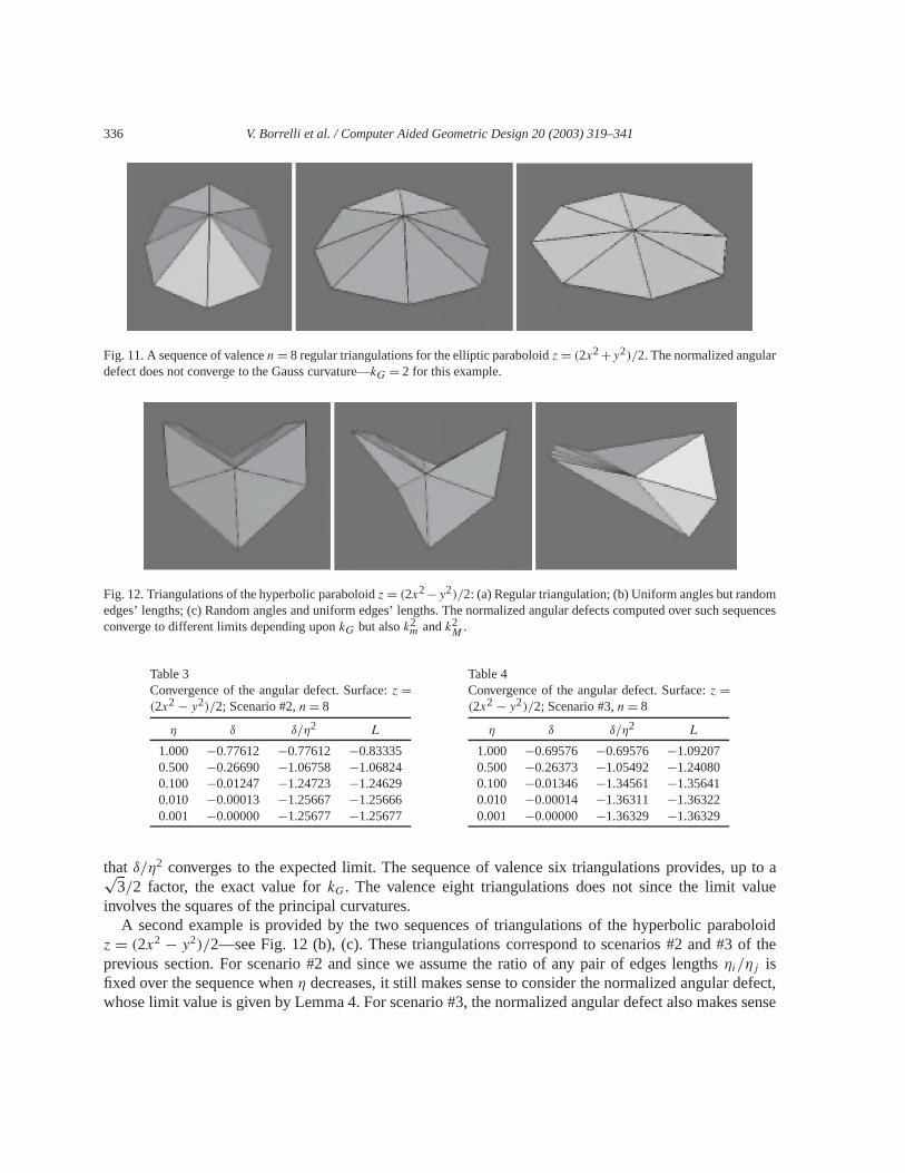
336 V. Borrelli et al. / Computer Aided Geometric Design 20 (2003) 319–341
Fig. 11. A sequence of valence n = 8 regular triangulations for the elliptic paraboloid z = (2x2 +y2)/2. The normalized angulardefect does not converge to the Gauss curvature—kG = 2 for this example.
Fig. 12. Triangulations of the hyperbolic paraboloid z = (2x2 −y2)/2: (a) Regular triangulation; (b) Uniform angles but randomedges’ lengths; (c) Random angles and uniform edges’ lengths. The normalized angular defects computed over such sequencesconverge to different limits depending upon kG but also k2
m and k2M
.
Table 3Convergence of the angular defect. Surface: z =(2x2 − y2)/2; Scenario #2, n = 8
η δ δ/η2 L
1.000 −0.77612 −0.77612 −0.833350.500 −0.26690 −1.06758 −1.068240.100 −0.01247 −1.24723 −1.246290.010 −0.00013 −1.25667 −1.256660.001 −0.00000 −1.25677 −1.25677
Table 4Convergence of the angular defect. Surface: z =(2x2 − y2)/2; Scenario #3, n = 8
η δ δ/η2 L
1.000 −0.69576 −0.69576 −1.092070.500 −0.26373 −1.05492 −1.240800.100 −0.01346 −1.34561 −1.356410.010 −0.00014 −1.36311 −1.363220.001 −0.00000 −1.36329 −1.36329
that δ/η2 converges to the expected limit. The sequence of valence six triangulations provides, up to a√3/2 factor, the exact value for kG. The valence eight triangulations does not since the limit value
involves the squares of the principal curvatures.A second example is provided by the two sequences of triangulations of the hyperbolic paraboloid
z = (2x2 − y2)/2—see Fig. 12 (b), (c). These triangulations correspond to scenarios #2 and #3 of theprevious section. For scenario #2 and since we assume the ratio of any pair of edges lengths ηi/ηj isfixed over the sequence when η decreases, it still makes sense to consider the normalized angular defect,whose limit value is given by Lemma 4. For scenario #3, the normalized angular defect also makes sense

V. Borrelli et al. / Computer Aided Geometric Design 20 (2003) 319–341 337
since ηi = η for all one-ring neighbors. The results are displayed on Tables 3 and 4. The concordancebetween the computed value and the theoretical one is that expected. The limits associated with the twotriangulations are different and involve the squares of the principal curvatures.
8. Conclusion
Let S be a smooth surface, p a point of S, and consider a mesh providing a piecewise linearapproximation of S around p. This paper establishes, asymptotically, several approximation resultsrelating the curvatures of S at p and normalized angular defects of meshes at p. In particular, weshow that the angular defect does not provide in general, an accurate point-wise estimate of the Gausscurvature.
From a practical standpoint, these results show that normalized angular defects should be used toestimate the Gauss curvature for these cases only where the geometry of the meshes processed is preciselycontrolled. From a theoretical perspective, we believe these contributions might find applications forthe many operations involving differential operators on meshes, that is fairing, smoothing, as well assubdivision. A clear understanding of the geometry of meshes in certainly one step forward more robustalgorithms.
On a broader perspective, these contributions illustrate the difficulties one has to face in orderto perform differential geometry on non smooth objects. It would therefore be very interesting togeneralize the analysis presented in this paper to all the methods—least-square quadrics, gradient-basedoperators, etc.—which are used to estimate the normal, mean curvature, principal directions, ridges, etcof triangulated surfaces.
Acknowledgements
The authors wish to thank Sylvain Petitjean for rereading this paper.
Appendix A. Proof of Lemma 1
Using spherical coordinates (x = η cos θ , y = η sin θ ) to express the position of a point p ∈ C, we getthat C is implicitly represented by F(η, θ) = 0 with
F(η, θ) = y − f (x) = η sin θ − f (η cos θ). (A.1)
Obtaining an expression of θ as a function of η involves the implicit function theorem applied to F at(η = 0, θ = 0). Unfortunately, ∂F/∂θ(0,0) = 0. We get around the difficulty using an auxiliary functionΦ defined as follows:
Lemma 5. Let Φ(η, θ) be defined by
η �= 0: Φ(η, θ) = F(η, θ)
η= sin θ − f (η cos θ)
η, (A.2)
η = 0: Φ(0, θ) = sin θ. (A.3)

338 V. Borrelli et al. / Computer Aided Geometric Design 20 (2003) 319–341
The function Φ is C2, and the point (η = 0, θ = 0) is a regular point of Φ. Moreover, near the originθ = Aη + Bη2 + o(η2).
Proof. The proof consists of three parts.Part I. Φ(η, θ) versus F(η, θ). We first observe that working with F(η, θ) or Φ(η, θ) is equivalent.
When η �= 0, the solutions of F = 0 and Φ = 0 are the same. If η = 0, the only solution of Φ = 0 is(0, θ = 0) which is also a solution of F = 0. To be more precise, any pair (0, θ) is a solution of F = 0,and working with Φ instead of F retains only one of these solutions, namely (0,0).
Part II. Φ(η, θ) is C2. To begin with, observe thatf (x) = kx2/2 + νx3/6 + o(x3) and f ′(x) = kx + νx2/2 + o(x2).
Using these two expressions in the following calculations are straightforward.Φ is C0.
limη→0
F(η, θ)
η= lim
η→0sin θ − f (η cos θ) = sin θ.
Φ is C1. We consider ∂Φ/∂η(0, θ) and ∂Φ/∂θ(0, θ) in the two settings—η �= 0 and η = 0.
• η �= 0, ∂Φ/∂η(0, θ)
∂Φ
∂η(0, θ) = lim
η→0
∂Φ
∂η(η, θ) = −k cos2 θ
2.
• η = 0, ∂Φ/∂η(0, θ)
∂Φ
∂η(0, θ) = lim
η→0
Φ(η, θ) − Φ(0, θ)
η= lim
η→0
(sin θ − f (η cos θ)
η− sin θ
)= −k cos2 θ
2.
• η �= 0, ∂Φ/∂θ(0, θ)
∂Φ
∂η(0, θ) = lim
η→0
∂Φ
∂θ(η, θ) = cos θ.
• η �= 0, ∂Φ/∂θ(0, θ)
∂Φ
∂η(0, θ) = ∂ sin θ
∂θ(0, θ) = cos θ.
Φ is C2. The equality of the four second order derivatives ∂2Φ/(∂u1∂u2) with u1 = {η, θ} and u2 = {η, θ}in the two settings are checked similarly.
Part III. Expression of θ as a function of (η). To see that (0,0) is a regular point, observe that∂Φ/∂θ(0,0) = cos 0 = 1. Since Φ is C2, applying the implicit function theorem yields
θ = Aη + Bη2 + o(η2). �The proof of lemma is now straightforward:
Proof. From Eq. (9), one easily derives the equivalents of cos θ and sin θ as a function of η.Plugging them into Eq. (4) yields Eq. (5). Eq. (6) is proved in the same way observing that pi−1 =(−ηi−1 cos θi−1, ηi−1 sin θi−1). �
V. Borrelli et al. / Computer Aided Geometric Design 20 (2003) 319–341 339
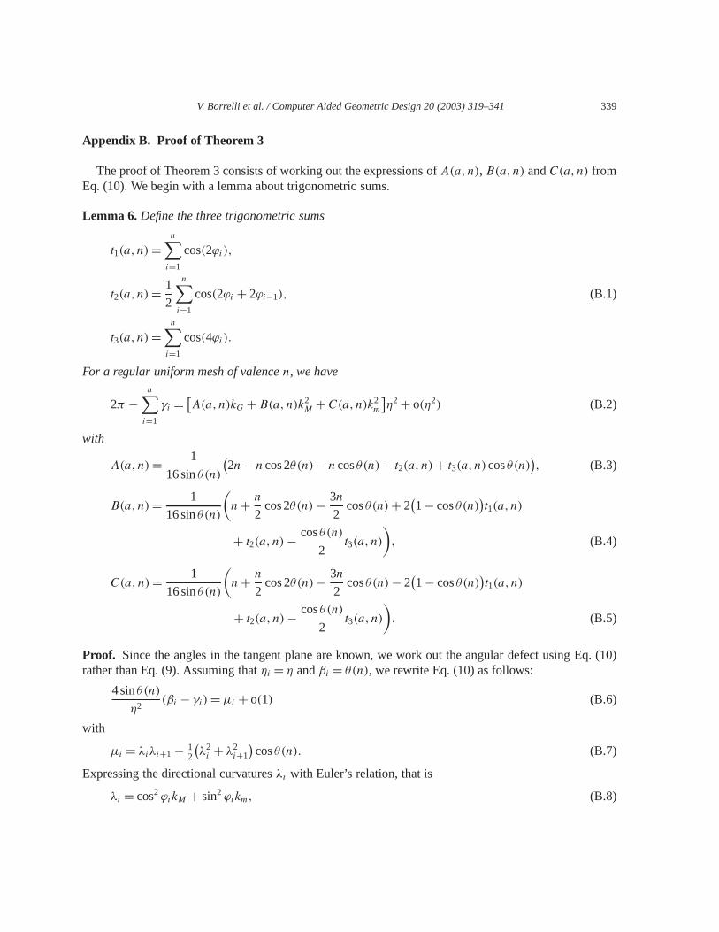
Appendix B. Proof of Theorem 3
The proof of Theorem 3 consists of working out the expressions of A(a,n), B(a,n) and C(a,n) fromEq. (10). We begin with a lemma about trigonometric sums.
Lemma 6. Define the three trigonometric sums
t1(a, n) =n∑
i=1
cos(2ϕi),
t2(a, n) = 12
n∑i=1
cos(2ϕi + 2ϕi−1), (B.1)
t3(a, n) =n∑
i=1
cos(4ϕi).
For a regular uniform mesh of valence n, we have
2π −n∑
i=1
γi = [A(a,n)kG + B(a,n)k2
M + C(a,n)k2m
]η2 + o(η2) (B.2)
with
A(a,n) = 116 sin θ(n)
(2n − n cos2θ(n) − n cos θ(n) − t2(a, n) + t3(a, n) cos θ(n)
), (B.3)
B(a,n) = 116 sin θ(n)
(n + n
2cos2θ(n) − 3n
2cos θ(n) + 2
(1 − cos θ(n)
)t1(a, n)
+ t2(a, n) − cos θ(n)
2t3(a, n)
), (B.4)
C(a,n) = 116 sin θ(n)
(n + n
2cos 2θ(n) − 3n
2cos θ(n) − 2
(1 − cos θ(n)
)t1(a, n)
+ t2(a, n) − cos θ(n)
2t3(a, n)
). (B.5)
Proof. Since the angles in the tangent plane are known, we work out the angular defect using Eq. (10)rather than Eq. (9). Assuming that ηi = η and βi = θ(n), we rewrite Eq. (10) as follows:
4 sin θ(n)
η2 (βi − γi) = μi + o(1) (B.6)
with
μi = λiλi+1 − 12
(λ2
i + λ2i+1
)cos θ(n). (B.7)
Expressing the directional curvatures λi with Euler’s relation, that is
λi = cos2 ϕikM + sin2 ϕikm, (B.8)

340 V. Borrelli et al. / Computer Aided Geometric Design 20 (2003) 319–341
and substituting into∑n
i=i μi yields a homogeneous polynomial of degree four in sines and cosines.We linearize this polynomial using the standard formulae cos2 a = (1 + cos 2a)/2, sin2 a = (1 −cos 2a)/2, cosa cosb = (cos(a+b)/2+cos(a−b))/2, as well as cos2 a sin2 a = (1−cos4a)/8, cos4 a =(cos 4a + 4cos 2a + 3)/8, sin4 a = (cos4a − 4cos 2a + 3)/8. Theses calculations simplify to Eqs. (B.3),(B.4) and (B.5).
Notice that the expressions of B(a,n) and C(a,n) just differ by the sign of the coefficient oft1(a, n). �Lemma 7. Let α an β be positive integers, and consider the sum
S(α,β,n) =n∑
k=1
cos(
α + kβπ
n
). (B.9)
If βπ/n = 0 mod 2π , then S(α,β,n) = n cosα. If βπ/n �= 0 mod 2π and βπ = 0 mod 2π , thenS(α,β,n) = 0.
Proof. If βπ/n = 0 mod 2π , the result is trivial. Otherwise, consider the two terms:
S(α,β,n) =n∑
k=1
cos(
α + kβπ
n
), T (α,β,n) =
n∑k=1
sin(
α + kβπ
n
). (B.10)
Let β(n) = βπ/n. Using complex numbers we have the geometric sum
S(α,β,n) + iT (α,β,n) =n∑
k=1
eiα(eiβ(n))k = ei(α+β(n)) 1 − einβ(n)
1 − eiβ(n)(B.11)
whose numerator is null if nβ(n) = βπ = 0 mod 2π . �We are now ready to prove Theorem 3:
Proof. To prove (1), we need to show that B(a,n) = C(a,n) in Lemma 6. Using the trigonometric sumof Lemma 7, we have t1(a, n) = S(2a,4, n), t2(a, n) = S(4a − 4π/n,8, n), t3(a, n) = S(4a,8, n).
But t1(a, n) = 0 for all values of n since, by the same lemma, we never have 4π/n = 0 mod 2π forn � 3. Since B and C just differ by the sign of the coefficient of t1, B = C for all ns.
For (2), A(a,n) and B(a,n) depend upon a if the trigonometric sums t2 or t3 are non vanishing.According to the above lemma the condition is 8π/n = 0 mod 2π , which occurs for n = 4 only.
For (3), it is easily checked that the only value of n such that B(a,n) vanishes is n = 6. �
References
Amenta, N., Bern, M., 1999. Surface reconstruction by Voronoi filtering. Discrete Comput. Geom. 22 (4), 481–504.Banchoff, T.F., 1967. Critical points and curvature for embedded polyhedra. J. Differential Geom. 1, 245–256.Calladine, C.R., 1986. Gaussian curvature and shell structures. In: Gregory, J.A. (Ed.), The Mathematics of Surfaces. Oxford
Univ. Press.Cheeger, J., Müller, W., Schrader, R., 1984. On the curvature of piecewise flat spaces. Comm. Math. Phys. 92.Cskny, P., Wallace, A.M., 2000. Computation of local differential parameters on irregular meshes. In: Cipolla, R., Martin, R.
(Eds.), Mathematics of Surfaces. Springer.

V. Borrelli et al. / Computer Aided Geometric Design 20 (2003) 319–341 341
Dyn, N., Hormann, K., Kim, S.-J., Levin, D., 2001. Optimizing 3d triangulations using discrete curvature analysis. In: Lyche,T., Shumaker, L.L. (Eds.), Mathematical Methods for Curves and Surfaces. Vanderbild Univ. Press.
Lafontaine, J., 1986. Mesures de courbures des varietes lisses et discretes. Sem. Bourbaki 664.Meyer, M., Desbrun, M., Schröder, P., Barr, A.H., 2002. Discrete differential-geometry operators for triangulated 2-manifolds.
In: VisMath.Morvan, J.-M., Thibert, B., 2001. Smooth surface and triangular mesh: Comparison of the area, the normals and the unfolding.
In: ACM Symposium on Solid Modeling and Applications.Meek, D.S., Walton, D.J., 2000. On surface normal and Gaussian curvature approximations given data sampled from a smooth
surface. Comput. Aided Geom. Design.Polthier, K., Schmies, M., 1998. Straightest geodesics on polyhedral surfaces. In: Hege, H.C., Polthier, K. (Eds.), Mathematical
Visualization.Reshetnyak, Y.G., 1993. Two-dimensional manifolds of bounded curvature. In: Reshetnyak, Y.G. (Ed.), Geometry IV. In:
Encyclopedia of Mathematical Sciences, Vol. 70. Springer, Berlin.Spivak, M., 1999. A Comprehensive Introduction to Differential Geometry, 3rd edn. Publish or Perish.Taubin, G., 1995. Estimating the tensor of curvature of a surface from a polyhedral approximation. In: 15th International
Conference on Computer Vision.Watanabe, K., Belyaev, A.G., 2001. Detection of salient curvature features on polygonal surfaces. In: Eurographics.