On Systematics in the 19F Electric Hyperfine Interactions

On Systematics in the 19F Electric Hyperfine Interactions

Michael Frank

Physikalisches Institut der Friedrich-Alexander-UniversitaÈt, Erlangen

Contents

1. Introduction . . . . . . . . . . . . . . . . . . . . . . . . . . . . . . . . . . 336

2. Method . . . . . . . . . . . . . . . . . . . . . . . . . . . . . . . . . . . . 337

3. Experimental Set-Up . . . . . . . . . . . . . . . . . . . . . . . . . . . . . . 3393.1. Accelerator and Beamstructure . . . . . . . . . . . . . . . . . . . . . . . . 3393.2. Electronics . . . . . . . . . . . . . . . . . . . . . . . . . . . . . . . . 3403.3. Target Preparation . . . . . . . . . . . . . . . . . . . . . . . . . . . . . 341

4. Experimental Results . . . . . . . . . . . . . . . . . . . . . . . . . . . . . . 3424.1. Results on Recoil Implantations. . . . . . . . . . . . . . . . . . . . . . . . 343

4.1.1. Carbon . . . . . . . . . . . . . . . . . . . . . . . . . . . . . . . 3454.1.2. Silicon . . . . . . . . . . . . . . . . . . . . . . . . . . . . . . . 3454.1.3. Germanium . . . . . . . . . . . . . . . . . . . . . . . . . . . . . 346

4.2. Results on Phase Transitions . . . . . . . . . . . . . . . . . . . . . . . . . 347

5. Model Based Description of the Electric Hyperfine Interaction . . . . . . . . . . . . . 3485.1. The Townes and Dailey Model . . . . . . . . . . . . . . . . . . . . . . . . 3495.2. The Bond Switching Model . . . . . . . . . . . . . . . . . . . . . . . . . 3505.3. Ab Initio Calculations . . . . . . . . . . . . . . . . . . . . . . . . . . . . 3505.4. Point Charge Calculations . . . . . . . . . . . . . . . . . . . . . . . . . . 350

6. Application of the Models to Experimentally Investigated Systems . . . . . . . . . . . 351

7. Model Based Determination of Electron Distributions in Covalent Bonded Molecules . . . 355

8. Temperature Dependence of the Hyperfine Parameters . . . . . . . . . . . . . . . . 3608.1. Temperature Dependence of the Coupling Constant nQ . . . . . . . . . . . . . . 3608.2. Temperature Dependence of the Observed Amplitudes . . . . . . . . . . . . . . 363

9. Systematics in Observed Hyperfine Parameters . . . . . . . . . . . . . . . . . . . 3689.1. Irregular Trend in Period III Fluorides . . . . . . . . . . . . . . . . . . . . . 3689.2 Reduced Charges in 3d-Transition-Metal-Trifluorides . . . . . . . . . . . . . . . 370

10. Mixed-Crystal-Systems . . . . . . . . . . . . . . . . . . . . . . . . . . . . . 377

11. Amorphous Systems . . . . . . . . . . . . . . . . . . . . . . . . . . . . . . 380

12. Concluding Remarks . . . . . . . . . . . . . . . . . . . . . . . . . . . . . . 382

Appendix . . . . . . . . . . . . . . . . . . . . . . . . . . . . . . . . . . . . . 383I. Simple inorganic fluorides . . . . . . . . . . . . . . . . . . . . . . . . . . 383II. Complex inorganic fluorides . . . . . . . . . . . . . . . . . . . . . . . . . 385III. Organic fluorides . . . . . . . . . . . . . . . . . . . . . . . . . . . . . . 385IV. Remarks . . . . . . . . . . . . . . . . . . . . . . . . . . . . . . . . . 386

References . . . . . . . . . . . . . . . . . . . . . . . . . . . . . . . . . . . . 386

Fortschr. Phys. 47 (1999) 4, 335ÿ388

1. Introduction

Fluorine chemistry is a field of growing interest and importance. This is due to severalfacts. The most general one is that fluorine is the most electronegative element. This ex-treme position in the periodic system of the elements is responsible for some unusual prop-erties. For example fluorine posesses only p-donor characteristics and no p-acceptor charac-teristics (GreV 94). Additionally in the ionic fluorine compounds there is always a welldefined coordination of the cations by the fluorine ions leading to well defined crystalswhich do not exhibit deviations from stochiometric compositions. Also the successes madein tayloring fluorine compounds and the possibility of growing high definition crystals aswell as mixed and amorphous phases of several fluorides, by powerful methods like hydro-thermal synthesis, chemical vapour deposition synthesis and ªchimie douceº synthesis, gavesome boost to the efforts in fluorine chemistry. A lot of these compounds, especially thetransition metal fluorides exhibit a huge variety of magnetic properties. Last but not leastthe theoretical treatment of fluorides is distinguished from other compounds due to theirrelative lucidity. However on the other hand there is a major drawback of fluorine com-pared to the other halides: according to the fact that the nuclear groundstate spin is I � 1/2it exhibits no quadrupole moment in this state. Therefore it is not accessible to NQR-spectro-scopy (Nuclear Quadrupole Resonance). This powerful method which was developed 1950 byH. G. Dehmelt and H. KruÈger (DehK 50, DehK 51) has meanwhile become an independentand essential tool in solid state physics. This method bases on the fact that the interaction ofan electrical quadrupole moment of the nucleus with an electric field gradient destroys degen-eracy of the m-sublevels of the corresponding energy level of the state. Between these energe-tically splitted levels transitions can be induced by irradiating them with an electromagneticfield the frequency (several kHz up to some GHz) of which corresponds to the energy differ-ence of the sublevels. So it is necessary that the nucleus under investigation posesses a non-vanishing quadrupole moment i.e. nuclear spin I � 1. However the condition of nonvanishingquadrupole moment is necessary but not sufficient. To induce transitions which can be de-tected as a resonance signal, the samples are irradiated with radio signals of the appropriatefrequency. It is therefore necessary that the level which is exposed to the electric field gradient(efg) has a lifetime which is long enough compared to the inverse of the resonance frequencyto enable the resonance to be detected and to give a linewidth and shape which is governednot only by the lifetime but by the specific environment of the probe nuclei. For this reason19F is not suitable for NQR. This means the NQR systematics can be performed for chlorides,bromides and iodines but not for fluorine, the most prominent halide.

However this problem can be solved at least in part by the TDPAD-method (Time Differ-ential Perturbed Angular Distribution). In this method the second excited level of 19F isexcited via the inelastic proton scattering reaction 19F(p,p0)19F*. This I � 5=2� level has anelectric quadrupole moment Q � 75 mbarn and a mean lifetime t � 128.8 ns. Due to kine-matic reasons the excitation of this 197 keV-level results in an alignment of the m-suble-vels, which in turn causes an anisotropic angular distribution of the g-radiation emitted bythe decay of the excited level to the groundstate. An interaction of the excited level with itsenvironment causes a time dependent perturbation of the angular distribution, which can bedetected by nuclear techniques. This technique works not only with 19F as probe nuclei.But 19F is the one which works best due to its moderate lifetime and the range of couplingconstants (nQ � 127 MHz). Besides this technical advantage there is also a structural one:In the investigation of fluorides the fluorine probe nuclei are a generic constituend of thesamples under test. Therefore no additional effects due to the probes obscure the results.The problems which may occur if the probe is no generic component of the sample can beseen in the interpretation of the experiments concerning recoil implanation into group IVelements. In these cases additional assumptions always have to be made on the location ofthe probes in the host lattice. Whereas in the case of fluorides it is a natural assumption that

M. Frank, 19F Electric Hyperfine Interactions336

the regular lattice sites are occupied. Another advantage is correlated with the nuclear spinI � 5=2 of the excited level. Due to this value there exist three pairs of sublevels(m � �1=2, m � �3=2 and m � �5=2). The three resulting transitions between make itpossible to measure the quadrupole coupling constant nQ and the asymmetryparameter hindependently from each other. This is for example not the case for the 35Cl NQR experi-ments were due to the value of I � 3=2 only the transition between the m � �1=2 and them � �3=2 sublevels can be observed and therefore only one combined experimental valueis accessible for the two quantities nQ and h, making it impossible to determine themindependently. So by use of the 19F-TDPAD method the systematics on halides can becompleted (Smi 86).

2. Method

The theory of electric quadrupole interaction has been described in the literature in fulldetail (i.e. Gub 88, RoÈs 88, ConB 87 see also refs. given herein). In the following sectiononly a brief outline of the basics is given.

The second excited level of 19F (t � 128:8 ns, Q � 75 mbarn, I � 5=2�) is populatedvia a 19F(p,p0)19F* inelastic proton scattering nuclear reaction by means of a pulsed protonbeam. Due to kinematic reasons the transfer of angular momentum differs in the directionof the beam compared to the plane perpendicular to it. This results in an alignment of them-sublevels belonging to the excited state i.e. sublevels with different jmj are populatednonequally. This alignment results in an anisotropic angular distribution W�q� of theg-radiation emitted in the transition to the groundstate. This distribution can be expanded ina series of Legendre polynomials Pi�cos q� :

W�q� �Pi

Ai � Bi � Pi�cos q� :

The coefficients Ai are given by transition matrix elements of the nuclear levels involved inthe decay. The factors Bi are given by Clebsch-Gordan-coefficients and the exact form ofthe alignment produced. Due to general invariance principles and the rules for the Clebsch-Gordan-Coefficients the indices are limited to even values i in the range of 0 � i � 2 � I. Inthe case of I � 5=2 considering the notation Aii ::� Ai � Bi the expression for W�q� be-comes

W�q� � 1� A22 � P2�cos q� � A44 � P4�cos q� :For a kinetic energy of �5 MeV it was shown that the coefficient A44 is approximately 3%of A22 and may therefore be neglected within the error bars for all practical purposes(KreN 78). So the angular distribution caused by the excitation with the beam is given by

W�q� � 1� A22 � P2�cos q� :The angular distribution and a fit according to the above function is shown in fig. 1.

The excited level can interact with its environment during its lifetime.The corresponding Hamiltonian Hel in the case of pure electrostatic interaction can be

written in the form:

Hel �P1

k� 0

4 � p2k � 1

Pkq�ÿk

�ÿ1�q � T�k�q � V �k�q :

Fortschr. Phys. 47 (1999) 4 337

Where T �k�q are the tensor operators of the electric multipole moments of the nucleus andV �k�q the multipole operators of the electric field. Due to the invariance under space inver-sion operations odd electric moments vanish. In the case q � 0 the coulomb interaction ofthe charge of the nucleus and the electric field at its location is described. Therefore onlythe origin of the energy scale is determined. In lowest order the terms with q � 2 yield asplitting of the m-sublevels due to the interaction between the quadrupole moment of thenucleus and an electric field gradient at its site. The q � 4 case describes hexadecupoleinteraction and is normally small compared to the quadrupole interaction. The splitting ofthe sublevels according to the electric quadrupole interaction is given by the energy eigen-values of the partial Hamiltonian for k � 2 which can be calculated by the secular equa-tion

Em

h � nQ

� �3

ÿ28 � Em

h � nQ

� �� h2 � 3� � 160 � �h2 ÿ 1� � 0 ;

where

nQ � e � Q � Vzz

4 � h � I � �2 � I ÿ 1� ; h � Vxx ÿ Vyy

Vzz

and Vii are the respective diagonal elements of the efg-tensor in its principal axis systemlabeled according to the relation jVzzj � jVyyj � jVxxj. In the case of axial symmetry�h � 0) the differences between the eigenvalues scale like 1:2 :3 whereas in the case ofh � 1 the relation changes to 1:1: 2. In the intermediate cases no such simple relationshold. Fig. 2 shows the splitting of the sublevels with h.

Because now the radiation from the excited level to the groundstate no longer comesfrom energetically degenerated sublevels the above shown splitting causes the angular dis-


Fig. 1: Angular distribution of the 197 keV g-radiation following the F(p,p0)19F* reaction(KreN 78)

tribution W�q� to be no longer static but to become time dependent

W�q; t� � 1� A22 � G22�t� � P2�cos q� :The perturbation factor G22�t� depends on the structure of the sample. In the case of poly-crystalline samples it is given by:

G22�t� �P3

n� 0s2n�h� � cos �wn�h� � t� ;

where w0 � 0 and wi, i > 0 labels the splitting of the three subleves expressed in frequencyunits. They are directly proportional to the product of the quadrupole moment of the probenucleus and the efg at its site. In real crystals the efg is not exactly the same for all equivalentlattice sites but exhibits a more or less small distribution. The assumption of a Lorentziandistribution of the efgs around their mean value results in a exponential damping of the cosinefunction. The same effect may occur for a exponential decay of the originally produced align-ment of the excited level. Finally the time dependent angular distribution can be written as

W�q; t� � 1� A22 � P2�cos q� � P3n� 0

s2n � exp �dn � t� � cos �wn � t� :

The aim of the experiment is to extract the time dependent fraction from W�q; t�, since thiscontains the data about the electric hyperfine interaction i.e. the coupling constant nQ, theasymmetry parameter h, the damping coefficients d and the effective amplitudes Aeff

22 .

3. Experimental Set-Up

3.1. Accelerator and Beamstructure

The proton beam is produced by means of the Erlangen EN Tandem accelerator. The nega-tive charged Hÿ-ions are prepared by a conventional duoplasmatron source. Since the timedependence of the 197 keV g-radiation is the quantity of interest the originally cw-beam ofthe accelerator has to be given an appropriate time structure. This is obtained by a twostage pulsing unit. At the low energy end (LE) of the accelerator (i.e. before the injectionof the beam into the accelerator) the LE-pulsing is done. This part mainly consists of a

Fortschr. Phys. 47 (1999) 4 339

Fig. 2: Variation of the splitting of the m-sublevels with increasing h

plate capacitor coupled to a dc-voltage which is interupted by a series of pulses with widthm < 100 ns and a repetition time of trep � 2 ms. This signal is also supplied to the detectionelectronics described later. After this unit the beam consists of pulses of width m equallyspaced with trep. This beam is now injected to the accelerator. After the acceleration at thehigh energy end (HE) of the accelerator the HE-pulsing unit is located. This comprises twoplates forming a capacitor which is coupled to a coil. This arrangement is tuned to form aresonance circuit with fres � 5 MHz. A rf of this frequency which is derived from the samemaster oscillator as the LE-pulses is fed to that circuit. The geometry is choosen in such away that the beam can reach the target only during the small time intervalls (tp � 5 ns)around the zero crossings of the rf which are spaced by 100 ns for a rf of 5 MHz. Bymeans of a delay between the rf and the LE-pulses one zero crossing can be made coinci-dent with the proton pulse leaving the HE-end of the accelerator. The beam produced con-sists of pulses with a width tp � 5 ns which are spaced by trep � 2 ms.

3.2. Electronics

The quantity which is measured in the experiments is not directly the time dependent angu-lar distribution but the superposition of W�q; t� and the exponential decay of the 197 keVlevel

N 0�q; t� � N0 �W�q; t� � expÿt

t

� �� U�q� � N�q; t� � U�q� :

This quantity is measured by a fast-slow coincidence circuit (see fig. 3). When the beamhits the target a few 19F(p, p0)19F* reactions take place besides a lot of other reactions. Thedecay g-radiation emitted subsequently by the sample is registered by two NaJ(TI) counters


Fig. 3: Schematic sketch of the experi-mental arrangement

located under 180� and 90� relative to the beam direction. The energy signals of thesecounters are fed to linear amplifiers and single channel analyzers to discriminate the197 keV radiation of interest. The output of the single channel analyzer is made coincidentwith the time signal from the respective counter. In contrast to the energy signals the timesignals have a good time resolution. Since the aim is to measure N(90�; t) and N(180�; t) itis necessary to have a well defined time at which the excited probe nuclei are prepared.Afterwards the next excitation has to wait until all the excited nuclei are back in thegroundstate. For this reason the time structure of the beam is choosen with tp � 5 ns. Thisis the range of counter time resolution of the counters and the repetition timetrep � 2 ms � 15 � t ensures that practically no excited nuclei are present at the time whenthe next excitation pulse hits the target. The output signals of the coincidence circuits are fedvia a mixer to the start input of a time to pulse height converter (TPC). The stop signal for theTPC is derived from the signal supplied by the LE-pulsing unit. Leading to an output signal ofthat TPC that is proportional to the time difference between the decay of a nuclear level andthe next pulse. But the pulses are equidistant and therefore this signal is also a measure for thetime between the excitation and the decay (i.e. the actual lifetime of the corresponding excitednucleus) as would be measured by changing the start and stop inputs of the TPC. This is notdone for practical reasons. In the experiments it turns out that the observed counting rates areseveral thousand counts per second compared to 500000 pulses per second. So only a fractionof about 1% of all pulses leads to a measured signal. The reason for this is the combination ofthe cross section of the excitation reaction and the small solid angle covered by the countersused for a good angular resolution. So in the case of changed TPC inputs the TPC would givea number of output signals which is �100 times the necessary one and therefore would con-siderably raise the deadtime of the analog to digital converter which prepares the signal for themulti channel scaler (MCS). Via a routing device the MCS discriminates from which counterthe actual signal originates and adds it to the appropriate spectrum.

The further data evaluation is done by a microcomputer. From the spectra taken under180� and 90� relative to the beam a ratio R�t� is formed:

R�t� ::� 2 � N�180�; t� ÿ c � N�90�; t�N�180�; t� � 2 � c � N�90�; t� ;

where c is a normalisation constant taking into account possible differences in the detectionefficiency of the 180� and the 90� counter. Using the expression for N�q; t� it turns outthat the relation R�t� � Aeff

22 � G22�t� holds. So by fitting the theoretical function on the rightside to the experimentally determined data on the left side of the equation yields the corre-sponding hyperfine parameters. The introduction of an effective amplitude is necessary dueto the fact that the observed amplitudes are reduced by the finete solid angle of the detec-tors and also due to physical effects as described for example in section 8.2.

3.3. Target Preparation

The experiments were mainly done under vacuum. The target preparation depends on theaggregate state of the sample material under normal conditions. The investigated materialscovered all three states. Ionic compounds mainly formed solids at room temperatur. In thiscase the material was filled into a small copper container. This was sealed on one face by acopper or Havar foil thin enough to allow the proton beam to pass through without consid-erable loss of energy. In these containers the material was exposed to the beam. For tem-perature dependent measurements the container was either mounted on a heating elementthe temperature of which was controlled electronically or on the cooling finger of a closed

Fortschr. Phys. 47 (1999) 4 341

cycle He-refrigerator. Hence a temperature range from 10 K up to 1000 K could be cov-ered. Covalent bonded compounds mainly form gases under normal conditions. Thereforethe compounds were sprayed carefully onto the cooling finger of the refrigerator at10 K±±20 K. This procedure caused the gases to freeze in form of molecular crystals. Afterthis shock-freezing procedure a thermal treatment just short of the sample's melting pointwas usually necessary in order to anneal crystal imperfections produced during the freezingprocedure. Some compounds in the regime between covalent and ionic crystals are liquidsat room temperature. However when the containers with the liquids are brought to vacuumin the target chamber they are vapourized due to the lowering of the boiling point. Theresulting gas is then frozen down in the same way as above explained for originally gas-eous compounds. Subsequently thermal treatment is necessary again.

Most of the sample material was bought as commercially available products of goodquality. However in several critical cases the samples were specially synthesized (SeF6,TeF6 with courtesy to Prof. Seppelt, Darmstadt; amorphous phases of GaF3 and FeF3 withcourtesy to Prof. Leblanc and Dr. Brulard, CNRS Le Mans). This was also the case for thehigh quality 3d-transition metal crystals as well as the mixed crystals of these compounds(courtesy to Prof. M. Leblanc and Dr. B. Brulard, Laboratoire des Fluorures URA 449CNRS, Univ. Le Mans). Hydrogen fluoride was produced shortly before the experiments bythermal decomposition of potassium hydrogen fluoride and supplied to the cooled targetfinger (courtesy to Prof. Breitinger, Erlangen for helpful advices on this topic). In severalcases, especially for the amorphous samples the sample structure was tested by X-ray struc-ture analysis after the experiments. For the samples containing iron MoÈûbauer spectroscopychecks (courtesy to Dr. J. M. Greneche, CNRS URA 807, Le Mans) were also performed.

4. Experimental Results

The TDPAD method was successfully applied to a lot of fluorides of the form EFn where Edenotes nearly all the elements in the main groups of the periodic system and a lot of thetransition elements. This allows to set up something like a periodic table of efgs.


Table 1Arrangement of the observed 19F-TDPAD-coupling-constants analog to the periodic table of elements.Most of the data given here and in the appendix are measured in Erlangen

HF40.1

LiF� BeF2 BF3 CF4 NF3 OF2# F2

3.8 21.0 30.22 59.9 82.7 100 125

NaF MgF2 AlF3 SiF4 PF3 SF6 ClF0 21.2 25.5 23.6 31.9 60.1 85.4

KF CaF2� GaF3 GeF4 AsF4 SeF6 BrF3

�0 3.1 30.7 36.23 32.8 55.7 71.5

RbF SrF2� InF3 SnF4 SbF3 TeF6 IF5

�4 3.4 25.8 28.9 26.4 42.7 37.8

CSF BaF2� TlF PbF4 BiF3

�5.6 2.5 10.5 23.8 13.9

all values in MHz, # predicted value, � several nQ due to different fluorine sites, � cubic structure,observed nQ due to radiation damage

Going from the upper right side of the table to the lower left one the covalent characterof the compounds decreases and simultaneously ionicity increases. With increasing ioniccharacteristic there is a general trend towards decreasing coupling constants. This trend isdue to the fact that with increasing ionicity fluorine approaches more and more a closedshell noble gas configuration of its electrons. A heuristic interpretation for this is the factthat in this situation the electronic configuration is, besides some perturbations due to polar-isation effects, nearly spherical and therefore does not contribute to the efg. Of course thisis only a trend, because the crystal structure also has effects on the efg. For example anucleus located at a position with cubic symmetry cannot be exposed to a efg due to sym-metry arguments, irrespective of the ionicity of its compound.

Plotting the efgs vs. the corresponding fluorine partners in a diagramm group by groupsome interesting systematics can be observed (fig. 4).

For example in the case of PF3, SiF4 and AlF3 the observed efg values are significantlylower than for the corresponding fluorides of their neighbours in the respective groups.Whereas this is not the case for ClF and probably for SF6 (for OF2 no experimental dataare available yet, however a prediction based on structural arguments yields a couplingconstant of nQ � 100 MHz). This trend cannot be understood in a simple model like theTownes and Dailey approach. However some more detailed calculations based on expliciteuse of wave functions optimized by a self consistent charge extended HuÈckel (SCCEH)method clearly can reproduce this trend (MisC 83).

In the appendix a table of the observed 19F-TDPAD data is given.More complicated structures like KFeF4, K2ZrF6, BaGeF6, F3BNH3 and a lot of organic

compounds like halomethane derivates have been investigated, as well.

4.1. Results on Recoil Implantations

Investigations in samples containing no fluorine as generic constituend were also performedwith 19F* also. This was done for carbon (graphite modification), silicon and germaniumsamples. The probe nuclei were injected into these samples by recoil implantation from thinCaF2 layers covering the targets. The interpretation of the obtained data can be based onthe knowledge of the efg values in the corresponding group IV tetrafluorides.

The kinetic energy of the pulsed proton beam was 5 MeV for the C-samples and2.8 MeV in the case of Si and Ge. The change to lower proton energies was necessary to

Fortschr. Phys. 47 (1999) 4 343

Fig. 4: Systematic variation of observed coupling constants. � indicates the predicted valuefor the OF2 coupling constant

avoid disturbance of the lifetime spectra by superposition of signals from parasitic nuclearreactions in Si and Ge due to the proton irradiation. Fig. 5 shows plots of typical R�t�spectra for C, Si and Ge samples. A compilation of results is given in table 2.

The targets used for the experiments were produced in different ways for the single andpolycrystalline samples. For the polycrystalline samples so called sandwich targets wereused. They consist of three layers. A thick Carbon layer that serves as a carrier is followedby the main sample (Ge, Si) which was vapour deposited onto the carrier. This layer thenwas covered by a thin vapour deposited layer of CaF2. From this last one the 19F* were


Fig. 5: R�t� spectra observed in C, Si and Ge. The spectrum b for graphite was taken with aproton dose 4 times the one according to spectrum a

Table 2Compilation of coupling constants observed in recoil experiments. In addition to the actualresults (t.w.) the data of Bonde-Nielsen are also given

Target structure Layer nQ1=MHz nQ2=MHz Ref.

Graphite p CaF2 57.0 42.8 t.w.

Silicon s LiF 34.7 23.0 BonL 84BF2 35.0 23.1

a LiF ÿ 22.5s CaF2 35.0 22.6 t.w.p ÿ 21.07

Germanium s CaF2 32.8 26.8 t.w.p ÿ 28.0s LiF 33.4 27.3 BonL 84

s � single crystal, p � poly crystal, a � amorphous. The column labelled Layer refers tothe material of which the thin layer was made from which the probe nuclei were implantedinto the samples

recoil implanted by means of the incident proton beam. In the case of single crystallinesamples the single crystals served as sample and carrier. For the graphite experiments thecarrier was polycrystalline graphite directly covered with CaF2.

4.1.1. Carbon

The carbon experiments were done on the graphite modification. In these samples twocoupling constants were observed. One with nQ � 57 MHz and h � 0:15 and a second onewith nQ � 42 MHz and an asymmetry parameter compatible with zero. The higher couplingconstant is in the same range as that observed for the C±±F-bond in fluoromethanes. Thereforethis coupling constant is assigned to a C±±F bond in graphite as well. To explain the occurenceof such a bond a reference to the crystal structure of graphite is made. This carbon modifica-tion consists of parallel stacked sheets of a planar network of six-membered carbon rings. Therecoil F is assumed to kick one of the C-atoms off its site and to form a C±±F-bond with one ofthe remaining carbon atoms, leading to a coupling constant of �57 MHz. This value isslightly smaller than the one observed for the C±±F-bond in CF4 (59 MHz). This reductionmay be due to the fact that in the present case the bond partners of the carbon bonded tofluorine are carbon atoms too. This can lead to a charge transfer to the fluorine atom resultingin a lowering of the observed efg. In CF4 all the bondpartners of the central C are F, compet-ing for the C electrons and therefore blocking the charge transfer. The asymmetry parameter isincompatible with zero and was determined to be h � 0:15. This deviation from axial symme-try is consistent with the electronic neighbourhood of the proposed F position. As a deloca-tized p-electron system exists which is built up from the non-hybridized Carbon-p-electronsperpendicular to the carbon planes, the efg-component in that direction can be expected to bedifferent from the corresponding in-plane component, resulting in a h-value different fromzero. In the carbon samples a second coupling constant of nQ � 42 MHz also occured. Thecorresponding amplitude increases with increasing irradiation time. Furthermore this secondfraction can only be fitted satisfactorily if an additional phase shift relative to the 57 MHzcomponent for that particular component is introduced. This phase shift is equivalent to a timedelay for the start of the quadrupole interaction of the 42 MHz component. Assigning thisfraction to a H-F fragment as done for other efg's in this frequency range (FraG 87), theobservations can be explained. The time delay may be due to the fact that hydrogen is nonatural constituend of graphite. Therefore hydrogen is only present in a small concentration,due to two reasons: a certain amount of H is injected by the proton beam used to produce the19F* probe nuclei. On the other hand graphite itself may contain some hydrogen due to itshydrogen storage capability and contact with agents containing hydrogen during the refine-ment of the graphite and the production of the samples. Since the diffusion coefficient ofhydrogen is about 107 times the one of fluorine (PalD 85, WalR 55), an interstitial F can beassumed to rest at its position while the H moves around in the sample. When such a H comesclose to the F it can be trapped to form a H±±F molecule, attached via a hydrogen bond to thecarbon lattice. Using some plausible assumptions on the H-concentration the average time a Fhas to wait until a H comes close, can be estimated to be in the range of 10±±30 ns. Using thisas the delay time in the fit yields good agreement with the experimental data. The correspond-ing time spectra are shown in fig. 5.

4.1.2. Silicon

In silicon two coupling constants can be observed: nQ1� 35 MHz and nQ2� 21ÿ22:5 MHz,all with h � 0. The experiments were done on single and polycrystalline samples. The35 MHz fraction could only be detected in the single crystalline samples.

Fortschr. Phys. 47 (1999) 4 345

Since in SiF4 the nQ value was determined to be 23 MHz, the observed 22.5 MHz frac-tion in the single crystals and the 21 MHz fraction in the polycrystalline samples wereassigned to a Si±±F-bond. The presence of such a bond can be explained by the capture ofprobe nuclei at dangling Si-bonds either present naturally or induced by the irradiationprocess. Due to the tetrahedrally crystal structure of Si such a F-probe nuclei trapped at adangling bond forms a F±±Si±±Si3 cluster with tetrahedral symmetry. Compared to the iso-geometrically SiF4 units a charge transfer towards fluorine may be enhanced in Si, due tothe missing competitors for the Si-electrons. This can explain the slightly smaller nQ valuesfor the Si±±F bond in Si samples compared to the one in SiF4.

The amplitude of the second fraction decreases with increasing temperature as observedby other groups (BonL 84). This behaviour may be interpreted as the annealing of a defect.Therefore the observed 35 MHz coupling constants is assigned to a defect structure. Forthis situation 3 structures may be thought of: The F-probe nuclei may either be located in aoctahedral or a tetrahedral interstitial position of the Si lattice. Or it may be located on asubstitutional lattice site. However due to the electronegativity of fluorine this last situationwould not be stable and would break into a configuration like the one assigned to the22 MHz fraction. Furthermore the symmetry of the 35 MHz fraction is parallel to the h111iaxis of Si. Therefore the octahedral position is not compatible with the experimental resultsand the assignment of the 35 MHz coupling constant to a tetrahedral interstitial position isleft. It is also known from other experiments that impuities in Si preferably occupy thetetrahedral position, in consistency with the above attribution (Brow 74, Wat 75, Wat 69,PicV 78). Bonde Nielsen (BonL 84) also gives evidence to the fact that the tetrahedralinterstitial position is not stable on longer time scales. A loss of alignment for the 35 MHzfraction in the TDPAD-spectra for times t > 1 ms approves this observation and givesfurther evidence to the choosen attribution.

4.1.3. Germanium

In the germanium single crystalline samples two efg's also occured. The correspondingcoupling constants are nQ � 27 MHz and nQ � 33 MHz. In the polycrystalline samplesonly one efg with nQ � 28 MHz is observable. In all cases the asymmetry parameter wascompatible with zero.

It might be assumed that the higher one of the two efg's is to be assigned to a Ge±±Fbond in F±±Ge±±Ge3 cluster in analogy to the F±±Si±±Si3 cluster in the silicon experimentssince Si and Ge have the same crystal structure. Also in GeF4 a coupling constant of35 MHz is measured which is close to the observed 33 MHz value. The smaller efg thenhas to be attributed to a tetrahedral intersitital position, just as in the Si case. However thisinterpretation leaves two problems unsolved:

1. Bonde Nielsen et al. also observed two efg's and in their temperature dependent ex-periments. They observed an increasing amplitude for the higher efg and a decreasing am-plitude for the lower one.

2. The symmetry of the 33 MHz efg was found to be in h111i direction. However if the33 MHz efg is due to a F±±Ge±±Ge3 configuration the forming of this complex is due to thepresence of dangling bond defects and due to an annealing effect their number shoulddecrease with increasing temperature. Also no prefered orientation of the danglig bondsshould be expected.

These problems can be solved assigning the efg's in the opposite way to the positions:the 27 MHz efg to the cluster configuration and the 33 MHz efg to the tetrahedral inter-stitial position. However then the relative large difference between the GeF4 efg valueand the one for the F±±Ge±±Ge4 complex has to be explained. However this can be asolid state effect caused by electrons from the environment of the configuration contain-


ing the probe nucleus. The size of the Ge atoms is about 30% larger than the one ofSi. Therefore the valence electrons are far more delocalized in Ge than in Si. Also thebandgap for the semiconductor Ge (Eg � 0:744 eV, LanB 82) is much smaller than thatfor the semiconductor Si (Eg � 1:17 eV, LanB 82). Since the experiments were done atroom temperature in the case of Ge some more electrons may be excited to the conduc-tion band and therefore serve as a kind of delocalized charge reducing the efg at theF-site.

4.2. Results on Phase Transitions

Another field of application for the TDPAD method is the investigation of phase transitions.In the section on the 3d transition metal trifluorides the magnetic phase transition in FeF3

will be discussed in some detail. Here two examples for structural phase transitions will begiven. The first one is observed in solid CF4. In fig. 6 the coupling constants for solid CF4

are plotted against the target temperature in the temperature range up to 70 K. The tempera-ture dependence of the efg is rather weak for temperatures up to 62 K. Above this tempera-ture the coupling constant strongly decreases. CF4 exists in a socalled a-phase below 76 Kand above this temperature the b-phase is stable (Gme 74). This transition temperature wasdetermined at atmospheric pressure. Therefore due to the fact that the TDPAD experimentswere done under vacuum and keeping in mind that the proton beam brings a thermal powerof �5 mW locally to the sample, the observed behaviour may be well interpreted as obser-vation of the transition between the a- and the b-phase of CF4.

However a more probable interpretation of the results is in terms of the observationsmade by Bol'shutkin et al. (BolG 72). These authors performed x-ray diffraction experi-ments in order to determine the crystal structure of solid CF4. Their samples were producedin a similar way as the ones used for the TDPAD-measurements: some gaseous materialwas frozen down by vacuum condensation at low temperatures (�8 K) and subsequentlyannealed at T � 45 K. When they heated the samples to temperatures T > 63 K they ob-served recrystallisation processes. This is exact the temperature range in which the TDPAD-experiments exhibit the break in the temperature dependency of the coupling constant. Withthe knowledge of recrystallisation processes this behavior can be understood as the result ofa smearing out of the efg due to the molecular dynamics and thus resulting in the lowercoupling constants.

Fortschr. Phys. 47 (1999) 4 347

Fig. 6: Variation of the observed coupling constant in CF4 with temperature

Another example for an observed phase transition is MnF3. In fig. 7 the correspondingcoupling constants are plotted vs. the target temperature. Up to 930 K the coupling con-stant is nearly constant at �28 MHz. Above this temperature two coupling constants withconsiderably lower values (approximately 10 MHz and 15 MHz) occur. These measure-ments were done first in 1989 (Fra 89). No polymorphous transition was known in theliterature up to 1080 K (Gme 77). Independently 1990 Bulou et al. observed a phasetransition with a hysteresis between 923 K and 940 K by differential thermal analysis(DTA) experiments (DanB 90). Up to now no details are known on the nature of thistransition. Since the transition temperatures observed in the DTA and the TDPAD experi-ments are close together there is some evidence that both kind of experiments probed thesame transition. Due to the fact that the TDPAD method is sensitive to the positions ofthe ions in the crystal it can be concluded that a structural phase transition has beenobserved.

5. Model Based Description of the Electric Hyperfine Interaction

As shown earlier the primary result of the experiments is the quadrupole coupling con-stant nQ. This is, apart from constants, given by the product of the electric nuclearquadrupole moment Q and the largest component of the diagonalized efg-tensor Vzz. Inorder to get information about the absolute efg it is necessary to known the value ofthe quadrupole moment. The first estimate of this value for 19F was given by Sugimotoet al. who combined experiments and calculations for CIF. The result was Q � 110 mbarn(Sugm 64). Mishra et al. improved this value and obtained Q � 72� 4 mbarn (MisD 82)which is within the error bars identical to the one of Kreische et al.(Q � 78� 5 mbarn, Barb 83) who used the coupling constant of solid fluorine (Barb 82)for the calculations. So the value of Q may be regarded as known and the task is leftto calculate the efg for a given compound in order to compare the calculation with theexperiment. Writing the efg-tensor in its explicite form and choosing the probe nucleusto be at the origin yields

Vzz�0� ��

r�r�r�3 cos2 qÿ 1� sin q dq dW dr :


Fig. 7: Temperature dependence of the coupling constant in MnF3

Provided the charge distribution r�r� around the probe nucleus is known, the correspondingefg can be calculated exactly. However normally r�r� is not known with the necessaryprecision. Therefore it is necessary to modify the above equation and to look for possiblemodels allowing to perform the calculations.

5.1. The Townes and Dailey Model

In the framework of the model of Townes and Dailey (DaiT 55) it is assumed that the efgacting on the probe nucleus mainly originates from its own electron shell with modifica-tions due to the actual bond situation in the molecule. Therefore the ansatz is made tofactorize the efg, i.e. the coupling constant nQ, by the atomic coupling constant times afactor taking into account the bond situation:

nQcov � nQat � �1ÿ i� � �1ÿ s� d ÿ p� � f � nQat

where i is the ionicity of the bond, s and d the amount of s and d hybridisation and p theamount of p-bonding. For s the empirical rule, s � 0:15 if the electronegatively differencebetween the bond partners exceeds 0.25, is given. For fluorine compounds this condition isalways fulfilled. The amount of d-hybridisation of fluorine is normally considerably lessthan 5% and can be neglected. The main problem is therefore to determine the ionicity i,the double bond character p and the atomic coupling constant nQat . This coupling constantcan be determined from the experiments supplying the efg of solid fluorine nQ � 127 MHz(BarB 82). Since F2 is completely covalent i equals zero. The same holds for s- andd-hybridisation and also no p-bonds are present in elementary fluorine. Therefore theF2-coupling constant equals, within the Townes and Dailey model, the atomic couplingconstant.

For other compounds if nothing else is explicitely known p is generally set to zero forfluorine. The determination of i is somewhat more awkward since there exists no exactdefinition of this term. A very wide spread formula was given by Pauling (Pau 45) whorelated the ionicity to the electronegatively (EN) difference between the bond partners:

i � 1ÿ exp ÿ 1

4� �XA ÿ XB�2

� �:

Doing so, the problem is shifted to the task to find an appropriate electronegativity scale.There exists one suggested by Pauling but there are also others introduced by Mulliken(Mul 34) or Allred and Rochow (AllR 58) and combinations of these (Hin 68).

In table 3 the EN-values of Pauling and Mulliken are given for F and Cl. In table 4 theresults of the calculated coupling constant for ClF for the different EN-scales are giventogether with the result of the ionicity i � 0:29 derived by Mishra et al. (MisD 82) for ClFfrom calculations based on molecular orbitals. The experimental value of the coupling con-stant is vQ � 86 MHz.

Fortschr. Phys. 47 (1999) 4 349

Table 3EN-values for F and Cl according to the EN-scales of Pauling and Mulliken

EN F Cl

cP 3.98 3.16cM 3.91 3.0

Table 4Results of TD-calculations on ClF based on dif-ferent values for the ionicity i

nQexp � 86 MHz nQcalc=MHz

ip 0.15 91.8iM 0.18 88.5

Compared to the experimental result the ionicity is overestimated by �6% by the EN-approach whereas it is underestimated by �10% by the molecular orbital approach. Sotaking into account that the error of the experimental data is at least 1±±2 MHz the agree-ment between the simple EN-based calculation and the experiments is satisfactory.

5.2. The Bond Switching Model

In this model the molecules are not treated as completely independent of their environment.The next neighbours are taken into account as well. In the case of fluorine probe nuclei thismeans that not only the effect of a bond with the central atom of the own molecule isregarded but also a certain possibility of a bond to an appropriate atom of a next neighbourmolecule. In other words the fluorine is allowed to switch its bond from one partner toanother one, thus blurring the assignment of the atoms to a special molecule. By this in theaverage the electron density at the fluorine site takes a more spherical shape compared tothe case of isolated molecules and that in turn results in a lowering of the efg. Howeverobtaining quantitative results is much harder than in the Townes and Dailey frameworksince the concept of switching bonds cannot be treated as straight-foreward as taking intoaccount ionicity and hybridisations which are given by scalar quantities whereas in theother case also the direction of the bonds has to be taken into account.

5.3. Ab Initio Calculations

In the past years more and more powerful computers have become available. This gavesome boost to CPU time intensive numerical methods. One of them is to locate electronwave functions at the atoms of the solid under investigation and treat as many parameters(positions of the atoms, form of the wave functions) as possible as free ones. Then theenergy of this arrangement is minimized by a self consistent Hartree-Fock-procedure. Withthe wave functions given by the final set of parameters the interesting quantities are calcu-lated as the expectation values of the according operators. For example the efg-componentVzz is calculated as

Vzz �Pij

�YiV̂zzYj dt :

The choice of the basis set for the calculations is a non trivial problem (see Moh 87, andreferences herein). When the LCAO-MO (Linear Combination of Atomic Orbitals-Molecu-lar Orbitals) is choosen very often Slater type orbitals are used. However for molecularcalculations the use of such functions leads to many-center two-electron integrals which arehard to evaluate. Therefore very often gaussian type orbital sets are used, due to their rathergoodnatured numerical behaviour and the fact that for those types the integrals can becalculated by an analytical procedure. When choosen carefully these functions give thesame results as the more realistic but also more complicated Slater type functions, but withconsiderably lower numerical efforts (Moh 87).

5.4. Point Charge Calculations

The models described above are suitable for more or less covalent compounds. Howeverthey become inadequate in the case of ionic crystals. In the case of the Townes and Daileymodel and the bond switching model the reason is that these models take into account the


ionicity only to reduce the efg produced within the molecule. Whereas the effect of extra-molecular changes is neglected. However in the case of ionic crystals (i! 1) these give themajor contributions. In the case of the ab initio calculations this could in principle be takeninto account, but the numerical effort necessary to describe ionic crystals by means ofindividual electron wave functions increases beyond the realizable limits.

A description of the ionic crystals which is more resonable is the point charge method.In a first step the solid is assumed to be built up from point charges located at the latticesites of the ions. The efg at the probe ion's site is then calculated as the sum over thecontributions of all other ions:

Vij � @2V

@xi @xj� 1

4 � p � e0�P

l

0 3 � xilxjl ÿ dij � r2j

r5l

!:

Where Vij is the ijth component of the field gradient tensor, i and j denote the x, y, zcomponents of the carthesian coordinates and l counts all the ions that contribute to the efg.By this the efg produced of all the other ions is given. However this efg also acts on theelectronic shell of the ion under investigation and may produce some deformation in itwhich in turn produces an efg at the nucleus' site. This additional efg is proportional to theefg acting on the electron shell and is normally much bigger than this one. This effect isdescribed by introduction of the so called Sternheimer (anti)-shielding factor g1:

V effij � �1ÿ g1� � Vij :

The values for the Sternheimer factor are given in the literature and depend on the methodthey are determined by and on the respective ions. For an isolated fluorine ion a value of30 is calculated (FowK 93). In solids the values �11 and �15 (FowK 93) are determined.For those fluorides for which point charge calculations have been performed in this workthe value g1 � ÿ10.6 (PasW 69) fitted best to the experimental results.

In order to achieve good convergence properties of the numerical procedure some carehas to be taken when the summation over the lattice positions is performed. For the calcula-tion of the efg it is effective to perform the calculations by shells of cells around the probenucleus. The cells have to be choosen in such a way that they have no monopolar and nodipolar moments.

Considering the solid to be built up of ions results in an efg at the lattice sites and also in anelectric field at the lattice sites. Since the ions at these positions have finite polarizability anelectric dipole moment is induced to them. This in turn effects the electric field at the latticeposition which again effects the induced dipole moments. This contribution can be taken intoaccount by a self consistent procedure which calculates the efg produced by the induced di-poles (TheC 81). The importance of these corrections strongly depends on the lattice struc-ture. In the case of KFeF4 (space group Amma) the effect of the induced dipoles is twice theone of the monopoles at the iron site. This is maily due to the polarizability of the fluorineions (a � 0:9 �Aÿ3 (TheC 81)) and the lattice positions at which they are exposed to a rela-tively high electric field. On the other hand at the fluorine site in the 3d-transition metaltrifluorides the dipolar contribution turns out to be an effect of less than 10% (BlaF 94).

6. Application of the Models to Experimentally Investigated Systems

The Townes and Dailey model was originally designed for two-atomic molecules. Howeverdue to the fact that in the fluorides fluorine is only bonded to one partner, in a first approx-imation it may be neglected for the efg at the fluorine site that the bond partner itself may

Fortschr. Phys. 47 (1999) 4 351

be bonded to other atoms as well (Smi 86). Therefore the model is also applied to biggercovalent bonded molecules. However as an inherent feature of these calculations no detailsof related componds can be reproduced. For example in the case of the fluoromethanessystematic variations of the efg with the bond partners of the central carbon can beobserved. Changes in the coupling constant from nQ(CHCl2F)� 58.2 MHz up tonQ(CClF3)� 60.6 MHz (FraG 86) can be found. The TD model gives a value of 64.7 MHzfor the C±±F-bond which is well within the range of the observed C±±F-efgs and may there-fore be taken as good zero order estimate.

In fig. 8 the calculated coupling constants are plotted versus the experimental ones forseveral fluorides. It turns out that with increasing ionicity the Townes and Dailey modeland the experiments differ more and more (this region is not shown in the plot). This canbe easily understood since in this model only the influence of the own molecule on the efgat the probe nucleus' site is regarded.

However with increasing ionicity the charge distribution due to the increasing ionic char-acter of the atoms has to be taken into account. In some more details this will be shownnow for the group V trifluorides NF3, PF3, AsF3, SbF3 and BiF3.

The results obtained for these compounds at 10 K are given in table 5.The additional 127 MHz coupling constant in NF3 is identical to the one observed in F2

within the experimental errors. Therefore it can be assumed that in a few cases F2 frag-ments are produced due to the irradiation process. This can be understood in the frameworkof a simple model taking into account the fact that the excited 19F* has a recoil energy of


Fig. 8: Plot of calculated versus ex-perimental coupling constants

Table 5Observed hyperfine data in the group V trifluorides

compound nQ=MHz A22=% h

NF3 82.7 5.3 0.07126.9 2.4 0.0

PF3 31.9 7.4 0.1AsF3 32.8 10.5 0.1SbF3 26.8 12.1 0.1BiF3 14.0 8.3 0.79

several hundred keV and it has to perform a replacement collision to be stopped at a sub-stitutional lattice site. During this slowing down some damages are produced and there is acertain chance that a F2 fragment might be formed. Such a behaviour was also observed inthe case of CF4 (FraG 86). In the cases of the other trifluorides a very small contribution(A22 � 1%, not listed in table 5) of an efg with nQ � 40 MHz can be found. This is identi-cal to the one observed in HF, indicating the forming of a small HF fraction in the samples.The presence of this fraction may be explained due to the fact that the compounds underinvestigation are hygroscopic. Water may therefore have been present in the samples. Theoccurence of a HF fraction can also be observed in nearly all compounds containing hydro-gen either as a natural constituend or as an impurity (FraG 87).

The nQ values given above can be compared to the results of a calculation in the frame-work of the TD-model. Table 6 gives the results for the calculations due to the model. Theparameter f 0 is calculated as the ratio between the atomic and the experimental efg values:f 0 � nQexp=nQat , the parameter f is the one introduced earlier: f � nQcalc=nQat . The calculatedvalues for nQcalc reveal in principle the trend of decreasing efg when going from NF3 to-wards BiF3 however except in the case of NF3 the numerical agreement between the experi-mental and the calculated values is poor. This is most likely the result of the increasingionicity (for NF3 i � 0:2 whereas for the other compounds it takes values up to 0.6). Forthe rather small amout of ionicity in NF3 the Townes and Dailey approach, taking intoaccount only the molecule under test itself, may be regarded as a good description. How-ever in the other cases with ionicity of 50%±±60% the effect of the charges in the environ-ment may no longer be neglected.

Another deficit of the Townes and Dailey model is the fact that is does not predict anyvalue for the asymmetry parameter h. In a covalent system this parameter is mainly deter-mined by the amount of p-bonds. The presence of p-bonds also lowers the coupling con-stant. However to explain the relatively low value h � 0:1 in the compounds NF3 to SbF3 ap-character of less than 3% is sufficient. This is also in agreement with the fact that exceptfor PF3 no remarkable deviation from a s-bond is reported (Hor 72, Waz 56). Therefore thefact is left that the calculated efgs are, except for NF3 which forms the most ideal molecu-lar crystal of the considered compounds, systematically to high. Since a underestimation ofthe ionicity seems not to be very likely this must be a solid state effect. At least for SbF3

this is supported by the results of a structure analysis (Edw 70). In this work it was foundthat different molecules are ªbridgedº by fluorine. Thus due to the bondswitching model alowering of the efg can be expected. In the case of NH3

14N microwave spectroscopy datafor the gas phase and 14N NQR-data for the solid state are available (SheG 50, MatS 65).The results are nQ � 7:07 MHz both for the gas phase and the solid state and thereforeindicating no significant solid state effect. Therefore the prediction of the TD-model fitsquite well to the experimental data in that case.

As can be seen as well in fig. 9 as explicitely in the numerical values of table 6 thecalculated efg values are systematically above the experimental ones; however a linear

Fortschr. Phys. 47 (1999) 4 353

Table 6Compilation of calculated coupling constants due to the TD model compared with the corre-sponding experimental results

compound nQexp=MHz nQcalc=MHz f f 0

NF3 82.7 86.7 0.68 0.65PF3 31.9 48.5 0.38 0.25AsF3 32.8 48.1 0.38 0.26SbF3 26.8 42.6 0.33 0.21BiF3 13.9 41.4 0.325 0.109

20.3 0.16

trend between the experimental and the calculated values can be stated. This overestimationcould be removed using a value of nQat � 100 MHz for the model predictions. Thereforethe measurement of the efg in F2 was a crucial experiment. F2 has completely covalentbond character and also no s and d hybridisation is present. Since the asymmetry parameterh was found to be zero also no p-bonds occur. Within the TD framework this yieldsnQat � nQexp (F2)� 127 MHz. This leaves the discrepancy of about 20% between the calcu-lated and the observed coupling constants unresolved.

Therefore also more elaborate ab initio calculations were performed for NF3, PF3, AsF3

and SbF3. BiF3 is not treated by these calculations since Bi is too heavy to be treated bythe implemented Hartree-Fock-procedure which does not take into account relativistic ef-fects which become important for heavier atoms. Additionally BiF3 is expected to form aionic crystal and is therefore a poor candidate for a wave functional approach. For thecalculations a gaussian 3-21G basis set was used. The calculations were performed at theCornell Supercomputing Center. The results are given in table 7.

The agreement between the calculated coupling constants and the experiments are quitegood in all cases and additionally also the h-values are reproduced quite well.

The last one of the group V trifluorides is BiF3. This compound forms a ionic crystalwith space group Pnma and lattice constants a� 6:5605 �A, b� 7:0155 �A and c� 4:8416 �A.The occupied point positions are 4c and 8d and fluorine is found in 4c and 8d positions(Gra 82). Therefore fluorine occupies two inequivalent lattice positions and two different


Fig. 9: Plot of the ratio f � nQcalc=nQexp vs. the EN difference of the corresponding com-pounds

Table 7Comparison between experimental data and the results of ab initio calculations

compound calculation (Sri 93) experiment

nQ=MHz h nQ h

NF3 71.7 0.07 82.7 0.07PF3 34.8 0.15 31.9 0.10AsF3 34.1 0.13 32.8 0.10SbF3 27# 0.15# 26.8 0.10

# preliminary result

efgs can be expected as observed in the experiments. With these data point charge calcula-tions were performed. For the Sternheimer antishielding the value g1 � ÿ10:6 of Pascha-lis and Weiss (PasW 69) was used. The results are given in table 8.

The numerical agreement between the calculated and the experimental efg-values is quitegood. Also the asymmetry parameters are reproduced to a satisfactory extent, thus indicat-ing that the description of that ionic compound in terms of point charges is adequate.

Summarizing this comparison between the results of different models allowing to calcu-late the efg and the corresponding experimental data it can be stated that the observedtrends in the efg with varying covalent resp. ionic character can be reproduced quite wellwith models like the one suggested by Townes and Dailey for covalent samples. However aprediction of the asymmetry parameter is not possible. The application of a point chargemodel for mainly ionic compounds yields satisfactory reproduction of the experimentaldata, but for all cases predictions at least 10% away from the experimental value have to beaccepted. The more elaborated ab initio calculations by means of a Hartree-Fock procedurecome somewhat closer to the experimental data but the numerical effort has to be increasedoverproportionally. This point however may be relativated more and more with the growingavailability of high performance workstations allowing ªdeskopº calculations today whichcould only be performed in big computer centers 10 years earlier (Pal 94). This trend seemsto continue and therefore ab initio calculations may even gain importance in the future.This will especially apply to those works that do not only regard the solid as a black boxthat has to be filled with bigger and bigger basis sets and optimized by elaborate programs.But those which calculate values by such a procedure that may by interpreted in terms ofphysically observable quantities like polarizabilities, dielectric constants, effective chargesand so on (Fow 93).

7. Model Based Determination of Electron Distributionin Covalent Bonded Molecules

Since the efg tensor Vij is determined by the charge distribution around the point of interestit seems to be natural to try to derive information on the charge distribution from theexperimentally accessible coupling constants. The charge distribution consists of a part gov-erned by the nuclei and another one governed by the electrons. Since it is generally impos-sible to unfold the integral leading to the efg-value, assumptions about the charge distribu-tion have to be made. In the framework of the TD model the major assumption is that theefg in covalent molecules is determined by the electronic shell of the probe nucleus andsome modifications to this due to the bond situation. Some additional arguments furtherreduce the possible contributors to the efg:

1. s-shells are spherically symmetric and therefore do not contribute to the efg at thenucleus;

2. full shells are also of spherical symmetry and their contribution therefore is zero;

Fortschr. Phys. 47 (1999) 4 355

Table 8Results of the experiments and the point charge calculations for BiF3

position calculation experiment

nQ=MHz r h nQ=MHz r h

4c 21.1 1.35 0.47 20.3 1.46 0.58d 15.6 0.83 13.9 0.79

r: ratio between the two efgs.

3. with increasing angular momentum and increasing main quantum numbers the contri-bution to the efg decreases rapidly.

Thus the main contribution is given by the open p-shell with the lowest quantum numbern. For 19F these simplifications result in the following formula for the total efg:

Vii �P

jajbjViij ;

where

Viij � hY2pjjV̂iijY2pj

i ; i; j 2 fx; y; zg :

ai are hybridisation coefficients and bi denotes the orbital occupation factor. Performingthe calculations for the efg tensor indicated in the above formula yields for the contribu-tions to Vzz :

Vzzz � Y2pz

3 cos2 qÿ 1

r3

�� Y2pz

� �::� q0 ;

Vzz�x; y� � Y2p�x; y�3 cos2 qÿ 1

r3

�� Y2p�x; y�

� �::� 1

2q0 :

For a completely filled 2p-shell these contributions sum up to zero as requested for a fullshell. The z direction is choosen to be along the s-bond. For all bond partners with aelectronegativity difference towards fluorine of more than 0.25 this s-bond is a sp-hybridorbital formed by the 2s and the 2pz orbitals of luorine. The corresponding hybridisationcoefficient takes the value 0.151=2. Due to the hybridisation four orbitals have to be takeninto account in the formula for the efg: the bonding and the antibonding sp-hybrid orbitaland the non-hybridized 2px and 2py orbitals

Y1 ��sp �Y2s �

��1ÿ sp

�Y2pz

Y2 ��1ÿ sp

�Y2s ÿ s �Y2pz

Y2 � Y2px

Y4 � Y2py :

However from the experiments only two quantities namely the coupling constant nQ andthe asymmetry parameter h are available. Therefore reasonable assumptions have to bemade for two of these coefficients: the antibonding sp-hybrid is assumed to be completelyfilled with two electrons and one of the px or py orbitals is arbitrarily choosen to be filledwith two electrons as well. A possible p-bond is then established with the other p orbitalsay py. Since the contributions to a filled shell sum up to zero the contribution of a missingcharge is the same but of opposite sign that for the same amount of charge in an emptyshell. Using this relation and denoting by sh and ph the amount of charge missing in thebonding sp hybrid and the py orbital and calculating Vzz and h (where h�jVxxÿVyyj=jVzzj)yields the two relations (Gub 88):

Vzz

q0� �1ÿ s� � sh ÿ 1

2ph ;

Vzz

q0� 3ph

2h:


Solving them for sh and ph supplies two equations for the missing charges in the corre-sponding orbitals:

Regarding an F2-molecule, no hybridisation is present. Since the electron configurationof F is 1s2, 2s2, 2p5 there is one electron missing in one of the p orbitals. This is perdefinitionem

sh � Vzz

q0�

1� h

31ÿ s

!; ph � Vzz

q0� 2

3� h ;

the pz orbital and therefore sh � 1 and ph � 0. Therefore the atomic efg Vzz at equals q0.This is consistently the same result as obtained before. The application of the above equa-tions allows model dependent determinations of electron distributions in covalent fluorides.

In fig. 10 the obtained sh-values are plotted for a variety of fluorides. For the period IIfluorides (the ionic compound LiF is not taken into account) the data are given explicitelyin table 9. In the third column of the table also the values for 1ÿ i (i � ionicity) are given.This quantity is zero for completely ionic compounds and takes the value 1 for completelycovalent samples.

The numerical agreement between the corresponding (1ÿ i) and sh values is quite good.In fig. 10 the datapoints are crowded around the diagonal in the plot of (1ÿ i) versus sh

indicating also good agreement between these two quantities.Since sh and (1ÿ i) both measure the covalency of the bond (a value of zero indicates a

completely ionic and a value of one a completely covalent situation) this correspondence

Fortschr. Phys. 47 (1999) 4 357

Fig. 10: Plot of (1ÿ i) values ver-sus sh-values

Table 9sh- and (1ÿ i)-values for several compounds

compound sh 1ÿ i

F2 1 1NF3 0.81 0.78CF4 0.56 0.53BF3 0.32 0.33BeF3 0.19 0.18

gives reliability to the results of the above sketched model because of the fact that bothquantities are calculated by a different ansatz but lead to the same result. Up to now themodel was only applied to the fluorine electrons. However if the quadrupole coupling con-stants and the values of the atomic coupling constants are measured for the other constitu-ends of the molecules the model can be used to determine the complete electron distribu-tion of the whole molecule. In CCl3F the 19F coupling constant was determined to benQ � 62 MHz and h � 0 by the TDPAD method. For chlorine the coupling constant wasdetermined by means of 35Cl NQR experiments (Fra 85). Three resonance frequencies werefound (fQa � 39:55 MHz, fQb � 39:9 MHz and fQc � 40:1 MHz). The occurence of threeslightly different coupling constants is a solid state effect due to the environment of themolecule in the crystal. Starting from the symmetry of the molecule all the three chlorinepositions are expected to be equivalent. Because of this reason and due to the fact that thedifferences between the three values are only small, for the following considerations anaverage value of fQ � 39:9 MHz is used. Since the nuclear spin of chlorine is I � 3=2,from the determination of the resonance frequency no seperation between the effect of theefg component along the principal axis in z direction Vzz and the asymmetry parameter hcan be made. The relation between the resonance frequency f and the coupling constant nQ

in the case I � 3=2 is given by:

f � 1

2� jnQj

��1� h2

3

� �s:

However even in the case of maximum asymmetry (h � 1) the correction due to the asym-metry is only 15% and in the case of h � 0:5 the correction reduces to less than fivepercent. Therefore in the following zero asymmetry is assumed leading to nQ � 2 � fQ� 79:8 MHz.

The result of the calculation of the corresponding orbital occupation with this value isgiven in table 10.

At the central carbon atom four sp3 hybrid orbitals are located which form together withthe sp hybrid orbitals of the halogen atoms the corresponding s bonds. Each single bondcontains two electrons. Therefore in the fluorine and chlorine orbitals (2ÿ sh) electrons arelocated whereas in the corresponding sp3 orbital the remaining sh electrons are to be found.CCl3F is widely spread and was of big technical importance until recently. Under the tech-nical names Freon�11, Frigen111 or simply R11 it was used as cooling medium in refrig-erators and as foaming agent.

After the check of the model in the cases of the simple fluorides it is also applied tomore complicated compounds.

Examples for those are trifluorobenzene C6F6 and trifluorotriazine C3N3F6 which areshown in fig. 11 (Gub 88).

These compounds are benzene derivates. In the first case hydrogen is substituted byfluorine. The observed coupling constant is nQ � 61 MHz, h � 0:09 (BerF 89) resulting insh � 0:58 e and ph � 0:03 e. In trifluorotriazine the hyperfine parameters were found tobe nQ � 57:7 MHz, h � 0:25 and the corresponding occupation parameters are calculatedto be ph � 0:08 and sh � 0:58. In these two cases the deviation of the efg from axial


Table 10sh-values for CCl3F for the fluorine and the chlorine site

probe 19F 35Cl

sh 0.57 0.855

symmetry can be understood remembering the structure of the compounds: they both arebuilt up from a benzene body and in the case of C3N3F6 every second carbon atom in thering is substituted by nitrogen. In the sixmembered C-ring a delocalized electron cloud isbuilt up from p-orbitals of the ring atoms not used to form hybrid orbitals for bonds withfluorine. Therefore the efg at the fluorine site is different in the directions parallel to thering plane and perpendicular to it. In the case of the C±±N-ring the electron distribution isalso different in the ring plane and perpendicular to it resulting in a non-vanishing asymme-try parameter.

Another interesting class of compounds for the determination of the electron distributionare the trifluoroaminoboranes F3BNH3 and their derivates of the type F3BNHx(CH3)3ÿ x.These compounds are of interest for at least two reasons. First the B±±N bond is the inor-ganic analogon of the C±±C bond in organic chemistry and is therefore of great interest tochemists. Second F3BNH3 is built up from borontrifluoride and ammonia. BF3 is a Lewisacid whereas ammonia is a Lewis base. This means in a simple picture that BF3 picks upan electron supplied by NH3 when the trifluoroaminoborane is formed. For that reasonF3BNH3 is also known as chargetransfer complex. Due to this charge transfer it could beexpected that the 19F coupling constant in F3BNH3 is significantly lowered compared toBF3. However the experiment does not show this. The quadrupole coupling constants arethe same within the experimental errors however the asymmetry parameter is changed bymore than 100% as shown in table 11. This behaviour can be explained when the calcu-lated occupation factors of both compounds are compared. For BF3 sh is already given

Fortschr. Phys. 47 (1999) 4 359

Fig. 11: Structural formulae and cuts fromthe electron distribution calculated for C6F6

and C3N3F6 (from (Gub 88))

Table 11Observed hyperfine data for BF3 and F3BNH3

sample nQ=MHz h

F3BNH3 30.3 0.2BF3 30.2 0.56

above, ph is calculated to be 0.09 e. For the calculation in F3BNH3 the coupling constantsfor 11B (nQ � 80 kHz (OllL 86)) and 14N have to be known. However the determination ofthe nitrogen coupling constant was impossible due to nitrogen and fluorine relaxation timesbeing too short for a double resonance experiment. However the coupling constants incorresponding H3BN- and F3BN-compounds are nearly identical (LoÈtV 84). Therefore in agood approximation the 14N coupling constant of H3BNH3 nQ � 1:5 MHz can be used.The result is the electron distribution shown in fig. 12.

It can be seen that the occupation of the s-bond in the trifluoroaminoborane is increasedat the fluorine site only by 0.03 electrons however the increase in the occupation of the py

orbital is 0.06 electrons compared to BF3. This is related to the dramatic change in theasymmetry parameter since for h the asymmetry in the efg components Vxx and Vyy is therelevant quantity and therefore the asymmetry in the occupation of the corresponding orbi-tals is changed by a factor of �2 if the asymmetry parameter does so. The change in thes-bond is only a small effect and partially compensated by the change in the py orbital.The change of the occupation in this orbital may be interpreted geometrically. In BF3 thecentral boron atom is sp2 hybridized and the molecule is planar. Perpendicular to the planeof the molecule there is the empty nonhybridized boron p orbital. Parallel to this is thenearly full 2py orbital of the fluorine. This may transfer part of an electron to the emptyboron orbital thus forming a partial p-bond as indicated by the high asymmetry parameterof h � 0:56. In F3BNH3 boron is sp3 hybridized. Therefore the bonds point towards thecorners of a tetrahedron with boron in the center. Additionally all orbitals are used to formbonds and therefore no empty boron orbitals parallel to the fluorine orbitals are available totake up electrons from the fluorine. This results in a drastic reduction of the asymmetry-parameter. In this simple picture the experimental data can be interpreted and connectedwith the results of the model dependent determination of the electron distribution.

8. Temperature Dependence of the Hyperfine Parameters

8.1. Temperature Dependence of the Coupling Constant nQ

The coupling constant in solids may vary with the temperature due to several reasons.There may be an explicite temperature dependence of the efg as shown recently by meansof the TDPAC-method for the semimetal system Sb1ÿ xMx (M� Sn, In, Ge, Ga, Cd, Zn,x � 0:05) (BlaF 94). Such an explicite temperature dependence can be understood in termsof changes in the conduction band and is therefore expected to be important in metals andsemiconductors or semimetals. However the extraction of the explicite temperature depen-dent term in the variation of the efg requires an investigation of these systems under exter-


Fig. 12: Electron distribution for F3BNH3

nally applied pressure and at varying temperatures. The application of external pressure inTDPAD-experiments is hardly possibly due to the necessity of an accessibility of the sam-ple under pressure to the proton beam. Therefore these effects are not investigated by the19F-TDPAD method in this work. This is also justified by the fact that fluorides normallyneither have metallic nor semiconducting properties.

Another mechanism for the variation of the efg with temperature is given by the thermalexpansion of the solids. This is most important in ionic crystals, since distances are directlyinvolved in point charge systems. As a typical example the temperature dependence of thecoupling constant in copperdifluoride (CuF2) is shown in fig. 13.

Since the lattice expands with increasing temperature nQ decreases. A linear regression tothe data points yields a slope of ÿ1:04 kHz/K. Since distances are involved in the electricfield gradient like rÿ3, a relative change of the lattice parameters of �18 � 10ÿ6=K can be

Fortschr. Phys. 47 (1999) 4 361

Fig. 13: Temperature dependence of the coupling constant in the ionic crystal CuF2

Fig. 14: Temperature dependence of the coupling constant in the molecular crystal CClF3

derived. Unfortunately no data on the thermal expansion coefficient in CuF2 were available.However the data for the copperchloride, -bromide and the iondine compound are21 � 10ÿ6=K, 20:7 � 10ÿ6=K and 24 � 10ÿ6=K (LanB 36) indicating that the estimate derivedfor the fluorine compound from the nQ evaluation is well in the right region.

In molecular crystals the temperature dependence of the coupling constants is muchstronger. An example is shown in fig. 14 where the nQ-values of CClF3 are plotted versusthe temperature T in the range between 10 K � T � 35 K.

In this case the coupling constant decreases by �2 MHz in a temperature range of 20 Kresulting in a temperature dependence hundred times stronger than in the case of ioniccrystals. This behaviour can be understood in the framework of a model taking into accountoscillations of the molecules in the crystal around their positions. A first approach in thisdirection was made by Dehmelt and KruÈger who regarded the molecules as a classicalrigid torsional oscillator (DehK 51). These torsional motion make the probe nuclei see anaveraged (smeared out) efg, resulting in a lowered coupling constant. However for hightorsional frequencies or low temperatures the classical limit is not longer valid. Bayer sug-gested a model based on a quantum mechanical harmonic oscillator in 1951 (Bay 51). Thismodel gives a better description of the observed data. Later Kushida (Kus 55) and Bayerand Kushida (KusB 56) expanded the model on other oscillatory modes (translations andaccoustic modes) leading to the so called Bayer-Kushida formula:

nQ�T� � nQ � 1ÿ 3h

8p2

Pni� 1

Ai

nTi

1

2� 1

exphnTi

kT

� �ÿ 1

0BB@1CCA

8>><>>:9>>=>>; :

Setting n � 1 the formula reduces to Bayer's model which is sufficient to describe the datain most cases. The line in fig. 14 shows the result of such a fit to the data.

In fig. 15 another typical case is shown. The parameters of the fit are the effective mo-ment of inertia, the torsional frequency and nQ�0�. The results for these values are withinthe expected range but some systematic deviations occur which cannot be solved comple-tely; especially the moment of inertia obtained by the calculations differs from calculations


Fig. 15: Temperature dependence of the efg in SeF6

made from the geometric data of the molecules by a factor up to three (Itt 85). Howeverone reason for this disagreement may be that the use of the Einstein model for the oscilla-tory motions in the molecular crystal is not sufficient. Another explanation may be that dueto intermolecular bonds which act as a kind of constraint the actual axis of the assumedtorsional oscillations may not coincide with an axis through the center of mass i.e. themoment of inertia calculated for a free molecule may be not correct for the actual situation.Some evidence to this explanation is given by the fact that for example in different halo-methanes the temperature dependence is quite different; a fact that can be explained by thepresence of hydrogen bonds.

In CHClF2 one hydrogen is present in each molecule. Between this hydrogen and thefluorine of neighbouring molecules hydrogen bonds can be formed, hindering the rotationalmotion. The results is a rather weak temperature dependence (see fig. 16). On the otherhand in CClF3 no hydrogen bonds occur, resulting in a much stronger decrease of the efgwith increasing temperature (fig. 14). However in any case the tendency described by themodel is consistent with the experimental data even when the obtained parameters may notbe directly identified as some classical parameters.

8.2. Temperature Dependence of the Observed Amplitudes

Besides the temperature dependence of the coupling constants described above i.e. the ob-served efg itself, also the corresponding amplitudes show a characteristic temperature de-pendence. Therefore the relation between the experimentally observed data and the theoreti-cal function is rewritten as:

R�t� ! R�t; T� � Aeff22 � G22�t� � f �T� � A22 � G22�t� :

The factorization by use of f �T� in the last step seems to be reasonable since all the otherterms depend only on nuclear properties (spin, alignment) and these may in a good approx-imation be regarded as independent of the temperature of the sample i.e. a quantity mainlyconcerned with the lattice but not with the nuclei in the sample.

In the case of ionic crystals the observed amplitudes are nearly independent of the tem-perature (see fig. 17) and rather high (10%±±15%) whereas in molecular crystals the ampli-

Fortschr. Phys. 47 (1999) 4 363

Fig. 16: Temperature dependence of the coupling constant in CClHF2. Due to hydrogenbonds the variation is rather weak

tudes strongly decrease with increasing temperature and are generally much lower than inionic crystals (2%±±8%) (see fig. 18).

This behaviour was not understood for a long time and was even expected to be theother way round (Haa 75): since in non metallic compounds the results were assumed to begoverned by radiation damage it was expected that at low temperatures no spectra could betaken whereas at higher temperatures the damage should be at least partly annealed andtherefore better spectra with higher amplitudes were expected. That this is not the case canclearly be seen in fig. 18 where the observed R�t; T� spectra are plotted for CClF3.

To understand this behaviour some attention has to be payed to the excitation process(BaF 91). When the proton beam impinges the target, in some cases the protons hit a fluor-ine and lift it to its second excited level via the 19F(p,p0)19F* reaction (many other pro-cesses take place also but are not relevant to the experiment). Due to kinematic reasons theexcited fluorine itself has a recoil energy of several hundred keV now and moves throughthe sample. In the following this fluorine is called projectile and others hit by it are referredto as targets. In the beginning of its path the projectile mainly looses energy due toelectronic processes; however at lower kinetic energies nuclear collisions become the domi-


Fig. 17: Observed amplitudes in the ionic crystal MnF3

Fig. 18: Amplitude variations in the molecular crystal BF3

nant processes. The transition between these two processes is continuous, however in thelater calculation for the sake of simplicity an abrupt transition at an energy Emax is as-sumed. In order to contribute to the signal resulting from a regular lattice site the projectilehas to come at rest at such a position. This can only be achieved by a replacement collisionof the projectile with a target fluorine since the number of F-vacancies produced by radia-tion damage is not high enough to contribute significantly to the observed signal by trap-ping a projectile to such a vacancy. Collisions between the F* projectile and target fluorinesare assumed to be elastic in the commonly accepted collision models. After the collisionthe target which was assumed to be at rest before the collision as well as the projectile haskinetic energy. The fate of the two particles now depends on the relation of these energiesto the energy Eb by which the target fluorine is bound to its position. In the case of ioniccrystals this energy is the binding energy in the order of magnitude of some electron voltsby which the ion is bond to the crystal. If the recoil energy of the target is less than Eb theprojectile moves on and can perform new collisions. If the recoil energy of the target ex-

Fortschr. Phys. 47 (1999) 4 365

Fig. 19: R�t� spectra of CClF3 for various temperatures. Clearly the improving quality ofthe spectra with decreasing temperature can be observed

ceeds the bond energy it can leave its lattice position. If simultaneously the remainingenergy of the projectile also exceeds Eb then both, projectile and target, move on and avacancy is left. However if the kinetic energy of the F* projectile after the collision is lessthan Eb it will be trapped to the free position and only the target moves on; a replacementcollision has been performed. In both cases in which a atom is located at the latice siteafter the collision the former kinetic energy of the atom has to be thermalized by thelattice. After a replacement collision the probe nucleus is now exposed to the efg at aregular lattice site and contributes to the corresponding fraction of the perturbation signal inthe angular distribution of the 197 keV g-radiation. The fraction fI of probe nuclei that per-forms a replacement collision within the framework of this model is given by

fI ��2 � x1�

p ÿ 2:295

x1

where x1 � Emax=Eb.The energy Eb is temperature dependent in principle; however thermal energies are in the

order of magnitude of some ten meV whereas Eb is typically in the order of eV and there-fore nearly no temperature dependence occurs. This results in the fact that the fraction ofnuclei that can perform a replacement collision is nearly independent of the target tempera-ture and therefore no temperature dependence of the amplitude occurs in ionic crystals.

In molecular crystals the collision kinetics are the same as for ionic crystals at the begin-ing However the energy Eb is now the bonding energy of the target fluorine to the corre-sponding molecule which is again in the order of eV. But when the replacement collisionhas been performed, a significant difference occurs. As mentioned above the kinetic energyof the trapped probe atom has to be thermalized after the trapping. So at first the energy istransferred to the molecule as a whole and from there to the surrounding lattice. If theremaining kinetic energy of the projectile is not small compared to the energy Ec by whichthe molecule is bond to the crystal this will result in a highly distorted local environment ofthe probe nucleus which is therefore not exposed to a well defined efg and thus does notcontribute to the obsered amplitude which will therefore be lower than in the case of anionic crystal.

Furthermore the molecule is bond to the lattice in a molecular crystal by weak van derWaals forces and therefore the bond energy Ec is in the order of several tens of meV up tosome 100 meV. Therefore thermal energies can effect the energy Ec significantly and astrong temperature dependence for the observed amplitude may occur for molecular crys-tals. These arguments can be put into analytical expressions (BlaF 91, Fra 89) leading to aformula for fM, the fraction of probe nuclei contributing to the observable amplitude inmolecular crystals:

fM �x2 � x1

x2

� �12

ÿ 1� 1

x2

� �12

� x2 � x2

x1

� �12

� ln ��1� x2�12 ÿ x1=2

2 �x1

;

where x1 � Emax=Eb, x2 � Ec=Eb.This function can be compared to the experimental data. Fig. 20 shows the normalized

temperature dependence f �T�=f �0� for IF5 and BF3 together with the curves obtained bythe model sketched above. A linear ansatz for the energies Ec�T� was made leading toEc�Ts� � 0 for Ts � 0:6Tm and 0.85Tm resp. A detailled analysis of the model (Fra 89)shows that the leading term in f �T� is determined by the squareroot of the ratioEc�T�=Emax. Therefore a better reproduction of the experimental data than in fig. 20 can beachieved by the use of a more complicated temperature dependence for Ec. However this


brings more free parameters into the model and of course with a higher number of param-eters, observed data can be reproduced in a better way.

Another interpretation of the situation might be in terms of a Debye-Waller-factor for akind of recoilless trapping of the projectile after a replacement collision or the effect mightbe attributed to radicals produced during the irradiation (Haa 91) but no quantitative resultshave been derived from such ideas. However there is an experimental result that gives someevidence to the assumption that the basic ideas of the suggested modell are right. In themodel it was shown that the main mechanism for the temperature dependence and thedifference in the amplitudes between ionic crystals and covalent bonded samples is givenby the two stage bond structure in the molecular crystals together with the rather lowvalues of the van der Waals energies providing the second stage bond energies. Therefore itshould be expected that the observable amplitude increases and its temperature dependencegets weaker if the covalent bonded units could be bound to the crystals by tighter bondsthan van der Waals bonds. This is the case in Na2PO3F. This compound is, besides forchecking the suggested model, of some technical interest, due to its fluorine content and itsbiological acceptability, as well. It forms ionic crystals where the cations are normal Na�ions. The anions however are (PO3F)ÿ ions which are molecular ions. These molecularunits are built of covalent bonds between their constituents. That is the reason why theobserved coupling constant takes the value nQ � 32 MHz which is within the error barsidentical with the one observed for the covalent P±±F bond in PF3 and also reproduced bythe calculations within the Towns and Dailey model.

Fortschr. Phys. 47 (1999) 4 367

Fig. 20: Normalized plots of the amplitudes of BF3 and IF5

Therefore in this compounds a situation is realized in which a covalent unit is bound tothe lattice by stronger (ionic) forces. As shown in fig. 21 the amplitudes are rather high butlower than that for ionic crystals and show a temperature dependence that is rather weakbut stronger than for a pure ionic crystal; as can be expected from the model.

9. Systematics in Observed Hyperfine Parameters

9.1. Irregular Trend in Period III Fluorides

Due to the fact that the electric quadrupole interaction has been measured for nearly allfluorides of the elements in the periodic table, systematics can be done over a great varietyof features.

Fig. 4 shows the observed coupling constants for several groups of the periodic sys-tem. It can be seen that when going from top of a group to the bottom the efgdecreases due to the increasing ionic character of the compound. However in all casesthe efg of the period III compounds is significantly lower than expected from an inter-polation of the other fluorides. Mishra et al. (MisC 83) performed selfconsistent chargeextended HuÈckel (SCCEH) calculations for the carbon, silicon and germanium com-pounds. Their numerical results are somewhat away from experimental values howeverthe general trend for the calculated coupling constants is the same as in the experi-ments. Recently Hartree-Fock-calculations were performed on these compounds (Cho 93)yielding the results shown in table 12 together with the experimental and the SCCEHdata.


Fig. 21: Temperature dependence of the observed amplitudes in Na2PO3F

Table 12Observed and calculated coupling constants for group IV tetrafluorides

compound nQ=MHz (Cho 93) nQ=MHz (MisC 83) nQexp=MHz

CF4 57.22 50.3 59.7SiF4 26.4 30.4 23.5GeF4 34.68 36.3 36.2

In the Hartree-Fock calculations gaussian basis sets were used. The results are closer tothe experiments and also confirm the trend observed. In their paper Mishra et al. arguedthat the dip in the efg for silicon may be due to the overlap integrals Sij between molecularorbitals i and j. With that quantities the size of the orbitals of the central atom in themolecules is taken into account. Therefore the geometry seems to be related to the observedeffect.

As shown for group IV members in fig. 22 this trend is not only valid for the fluoridesbut also for the corresponding chlorides, bromines and the iodine compounds. Therefore theassumption that the effect is caused by a special feature of fluorine may be excluded. Dueto the different sizes of the halides a simple geometric argumentation seems to be unlikelytoo. It may be more probable that the origin can be found in the period III elements them-selves. In fact these elements have values for several quantities, which are higher or lowerthan the ones expected from the interpolation of the values of their neighbours in the peri-odic table of elements. In fig. 23 this is shown for the binding energy.

But similar plots can be made for other features, for example the electronegativities, aswell. Therefore the reason for the unexpected properties seem to be intrinsic to these ele-ments. However no argument has been found up to now, which assigns the 3p shell, whichstarts to be filled in the elements that show these effects, a special importance.

Fortschr. Phys. 47 (1999) 4 369

Fig. 22: Reduced coupling constants f � nQ=nQat of the group IV tetrahalides

Fig. 23: Irregular trends in period III binding energies. Data from (Hug 53)

9.2. Reduced Charges in 3d-Transition-Metal-Trifluorides

The trifluorides of the 3d-elements Ti, V, Cr and Fe are isostructural and crystallize in therhombohedral space group R�3c at room temperature. Scandiumtrifluoride is also reported tohave the same structure (Now 39) however some authors also report different structures inthe literature (LoÈsH 82, Redp 83). Since ScF3 completes the systematics to the left in theperiodic table it is also taken into account in the following systematics.

The crystals are built up of corner sharing MF6 octahedra (M � Sc, Ti, V, Cr, Fe). Thearrangement of these units is slightly different in the high temperature and the low tempera-ture phase. At high temperatures the octahedra form a cubic network. Below the transitiontemperature Tc the MF6 octahedra are tilted by an angle wn around the three-fold axis ofthe cubic cation sublattice and then exhibit the space group R�3c.

The transition temperature Tc is above room temperature for all compounds investigated.In fig. 24 typical R�t� spectra for the MF3 (M � Sc, Fe, V, Cr) compounds are shown atroom temperature. For FeF3 the 525 K spectrum is shown. The reason for this is the factthat in the compound not only a structural phase transition exists but also a magnetic one.Below the NeeÂl-Temperature TN � 363 K irontrifluoride is a weak antiferromagnet whereasabove TN no magnetic ordering is present. Since in the magnetic phase no modulationpattern can be observed for polycrystalline samples and large single crystals were not avail-able, the experiments were performed above TN. Table 13 shows the results of the TDPADexperiments together with some structural data.

For irontrifluoride the experiments were performed also in the temperature region closeto the NeeÂl point. Fig. 25 shows the values for the amplitudes observed in this case.

The decrease of the amplitude when T approaches TN may be interpreted in terms of anonset of shortrange magnetic order probed at the anion site in the crystal. When magnetic


Fig. 24: R�t� spectra for some transi-tion metal trifluorides

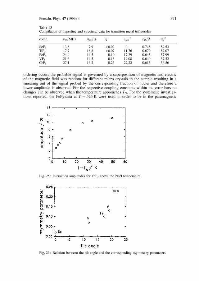
ordering occurs the probable signal is governed by a superposition of magnetic and electricof the magnetic field was random for different micro crystals in the sample resulting in asmearing out of the signal probed by the corresponding fraction of nuclei and therefore alower amplitude is observed. For the respective coupling constants within the error bars nochanges can be observed when the temperature approaches TN. For the systematic investiga-tions reported, the FeF3-data at T � 525 K were used in order to be in the paramagnetic

Fortschr. Phys. 47 (1999) 4 371

Table 13Compilation of hyperfine and structural data for transition metal trifluorides

comp. nQ=MHz A22=% h wn=� rM=�A a=�

ScF3 13.8 7.9 <0.02 0 0.745 59.53TiF3 17.7 16.8 <0.07 11.76 0.670 59.07FeF3 24.0 14.5 0.10 17.29 0.645 57.99VF3 21.6 14.5 0.13 19.08 0.640 57.52CrF3 27.1 16.2 0.23 22.22 0.615 56.56

Fig. 25: Interaction amplitudes for FeF3 above the NeeÂl temperature

Fig. 26: Relation between the tilt angle and the corresponding asymmetry parameters

phase. Since the crystal structure is the same for all investigated compounds the effect ofstructural parameters on the hyperfine parameters can be studied.

In fig. 26 the variation of the asymmetry parameter h with the tilt angle wn is shown.With increasing wn the deviation of the fluorine sites from axial symmetry increases. Thisis seen in the h-value increasing from a value compatible with zero for ScF3 which isreported to be (nearly) cubic (wn � 0�) up to h � 0:23 for CrF3 with a tilt anglewn � 22:22� which is the crystal with the highest tilt angle in this series.

Similar systematics can be found for the coupling constant itself. With increasing latticeconstants the observed efg decreases, as expected for ionic crystals. The data do not fit to aline given by the cube of the distances due to the fact that from one compound to the nextnot only the interatomic distances change but also the tilt angle and therefore the Vxx and Vyy

components of the efg tensor vary too. However the general trend of decreasing efg withincreasing distances is well reproduced (fig. 27). Besides the correlations between the ob-served hyperfine parameters and the structural parameters some additional systematics can befound, relating the hyperfine parameters and the electronic configuration of the cations.

In fig. 28 the observed coupling constants are plotted versus the number of 3d electronsof the cation atoms. From scandium to chromium with increasing number of 3d electronsnQ increases too, however the efg value of FeF3 breaks this trend. In fig. 29 the correspond-ing cation radii ri are plotted against the number of 3d electrons and the wellknown trend is


Fig. 27: Variation of the efg with lattice constant

Fig. 28: Correlation between coupling constants and # of 3d electrons

seen that with increasing number of 3d electrons, i.e. going within the period from the leftto the right, the corresponding cation radii decrease from scandium to chromium. For theFe3� ion there exist two electron configurations. The low-spin configuration for which thetrend of decreasing radii is continued and the high-spin configuration for which the ionicradius is considerably higher than for the low spin configuration. Extrapolating the trend ofincreasing efg with decreasing ri for the low spin configuration a nQ of about 32 MHzcould be expected. The experimental value however is 24 MHz and therefore close to theone observed for VF3 where it can be expected to be for the Fe3� high-spin configurationsince the corresponding ionic radius is also close to the V3� value. The same trends can beobserved for the asymmetry parameter h. For the low-spin configuration a h-value of about0.5 can be extrapolated which is well off the experimentally observed value of h � 0:1which is again close to the corresponding VF3-value.

Therefore from the 19F hyperfine data the conclusion that in FeF3 the Fe3� ion is in thehigh-spin state can be drawn. This is compatible with the results from 57Fe MoÈûbauerexperiments.

In an earlier paper (BarB 80) a statement of the observation of such a behaviour wasmade. However neither the details of the crystal structures nor of the actual electronic con-figuration were taken into account.

In principle the same argumentation as above could be applied to MnF3 for which theexperiments yield nQ � 28:5 MHz and h � 0:18. In this case again the high-spin configura-tion is favored by the TDPAD-data. However MnF3 has a monoclinic structure with spacegroup C2/c-C6

2h (Nr. 15) (Gme 77). In this structure five inequivalent fluorine positions ex-ist. Point charge calculations show that the efgs on these sites are slightly different. Thisexplains the spectra which can be fitted only with a relative high damping parameter. Thiscan be interpreted in terms of slightly different efgs which cannot be resolved in the experi-ment. Due to the fact that MnF3 has a different crystal structure than the other compoundsthe inclusion of that sample to the systematic may be regarded questionable. On the otherhand the classification by space groups gives much weight to possible symmetry operationsin the structure whereas for the efg mainly the positions are relevant. In the case of MnF3

the crystal is also built up of corner sharing octahedra like in the rhombohedral compounds.However the octahedra are distorted resulting in symmetry operations different from theones included in the R�3c class and also in slightly inequivalent lattice sited in contrast tothe situation in the rhombohedral structure were only one fluorine position is present.Therefore the inclusion of MnF3 in the systematics may be reasonable, provided not toomuch weight is put on the exact numerical data.

Fortschr. Phys. 47 (1999) 4 373

Fig. 29: Plot of cation radii versus the number of 3d electrons

For the MF3 compounds mentioned above point charge calculations were performed too.The program used was a modified version of the algorithm supplied by J. Theillet(TheC 82). The calculations were performed in direct space and the crystals were built upof successive shells of unit cells. Care was taken to obtain cells with zero monopolar anddipolar moments. Additionally possible contributions of induced dipole moments weretaken into account. For the calculations full ionic charges (i.e. �3 for the cations and ÿ1for the anions) were used. First the results for M � Sc, Ti, V, Fe and Cr are shown infig. 30 where the calculated efgs are plotted versus the experimentally observed ones. Theopen circles indicate the results of the calculations using full ionic charges whereas the fullones give the results of reduced charge calculations. The triangles correspond to the pre-dicted values for the reduction factors. It turns out that the calculated values differ stronglyfrom the experimental ones; however the asymmetry parameters are reproduced to a satis-factory extent. The disagreement between the calculations and the experimental data couldbe removed by the use of a set of reduced charges, keeping the neutrality condition3 � QF � QM � 0 (BlaF 94). For CrF3, VF3 and FeF3 such a set of reduced charges wasalready determined in the explanation of lattice dynamics data (DanB 90). In these experi-ments the Raman spectra recorded at room temperature can be described by a rigid ionmodel with a superposition of short range interatomic forces and coulombian ionic interac-tions. The calculations consist in fitting the model to the Raman line positions assuming


Fig. 30: Plot of calculated efg vs.experimental ones

Fig. 31: Variation of the reduc-tion factors with the correspond-ing number of 3d electrons. Opencircles: values from DanB 90, fullsymbols t.w.

free force constants for the short range forces and free charges for the ions. This leads to aset of reduced charges. The use of these reduction factors in the pointcharge calculationsgives nearly perfect agreement between the observed TDPAD-data and the calculations (seefig. 30). The variation of the reduction factors with the number of 3d electrons reveals thecorresponding behaviour of the efg (fig. 31).

The applicability of the reduced charges from the Raman experiments to the TDPAD-data may be interpreted in the other way round too and therefore in the case of ScF3 andTiF3 a reduction factor can be deduced from the TDPAD-data (table 14).

This leads to a prediction for the reduced charges expected to be necessary to describethe results of Raman experiments in these two compounds which have not yet been per-formed. The necessity of the reduction factors can be at least in part attributed to a partiallycovalent character even of the ionic compounds as stated already by Greenwood (Gre 73).However no numerical data were given. It also has to be stressed that the reduced chargesnecessary to bring the calculations and the experiments together may not be interpreted interms of real charges located at the lattice positions of the ions. In the contrary keeping inmind the relation proposed by Pauling (Pau 45) �i � 1ÿ exp �ÿ0:25 � Dc2�� that relatesthe ionic character i to the electronegativity difference Dc between the constituends of thecompounds, the ionicity decreases from scandium to the right in the periodic system(fig. 32).

In the pointcharge calculations the experimentally determined distances are used. How-ever these distances are already affected by covalency effects. This leads to a kind of self-compensation of the decrease in ionicity as shown in fig. 33. Here the quantity i=d3 isplotted versus the number of 3d electrons of the cations. This term is a measure for the

Fortschr. Phys. 47 (1999) 4 375

Table 14Reduction factors for the investigated transition metal trifluorides

M3� red. factor reference

Sc3� 0.38 this workTi3� 0.49 this workV3� 0.665 DanB 90Cr3� 0.795 DanB 90Fe3� 0.683 DanB 90

Fig. 32: Pauling ionicity as function of the number of 3d electrons

leading terms in the pointcharge calculations when the ionicity i is used as a reductionfactor. The typical increase from scandium to chromium and the low iron value is repro-duced quite well. All these arguments show the necessity of the use of reduced chargesinstead of the full values given by the oxidation numbers. However no direct deduction ofthe exact numerical values for the reduction factors can be found. Reduced charges withreduction factors considerably less than one have to be used for the MF3-compounds(M � Sc, Ti, V, Cr, Fe) whereas in the cases of BiF3 or SnF4 and other ionic compoundsgood results are obtained with values close to the full charges. This may be taken as evi-dence that this behaviour is related to the character of the open 3d-shell. To test this as-sumption and also to check whether the presence of open d-shells irrespective of the mainquantum number is sufficient, measurements on the 4d trifluorides RuF3, RhF3 and PdF3

seem to be interesting, as these crystallize also in the rhombohedral R�3c space group.In spite of the reservations on the applications of results from the R�3c-compounds to

MnF3 due to the reasons given above, the concept of reduced charges was also applied tothis compound. The result of the point charge calculation is shown in table 15. The valuescalculated for the coupling constants are close together and cannot be resolved in theTDPAD-experiments. Therefore the average is taken over all five data sets resulting in�nQ � 1:29 (in rel. units) and �h � 0:14. On the other hand Mn has four electrons in the 3dshell and is therefore located between chromium and iron. Since no value for the reductionfactor is known from Raman experiments, a rough estimate for MnF3 is taken. Averagingbetween chromium and iron values for the reduction factor leads to a Mn-value of 0.74,which can again be regarded as a prediction for a reduction factor to be tested by futureRaman experiments on this compound. With the above reduction value a coupling constantof 28.8 MHz is calculated for MnF3 which is in a quite good agreement with the experi-mental value of nQ � 28 MHz and h � 0:18. Since the reduction factor 0.74 is only arough estimate and from the value of the Mn3� cation radius also a reduction factor closeto the iron value could be assumed the good numerical agreement between the calculation


Fig. 33: Plot of the leading term in the pcc versus the number of 3d electrons

Table 15Results of the pcc on MnF3

MnF3 nQ=rel. units 1.28 1.31 1.28 1.30 1.30

h 0.152 0.128 0.149 0.125 0.129

and the experiment should not be overestimated. However the fact that in the MnF3 case areduction factor is also necessary and that its value seems to be quite reasonable givessome reliability to the concept of reduced charges.

This concept is not restricted to the special crystal structure of the binary transition metaltrifluorides. A somewhat more complicated structure is the one of KFeF4 which crystallizesin the space group Amma (D17

2h) (TeiC 82). There are three inequivalent fluorine positions inthis structure with relative frequencies 1:1:2. Table 16 shows the normalized results of thecalculations and the experiments. For the fit of the experimental data the values of theasymmetry parameters were fixed to the ones obtained from the calculations in order toobtain better convergence.

For better readability the coupling constants were normalized to the value of nQ3,whereas the amplitudes were normalized to A22; 2. It can be seen that the normalized valuesof the calculations and the experiments fit together quite well.

Using the reduction factor 0.683, valid in the FeF3 Raman- and TDPAD-experiments, forthe pointcharge calculations (pcc), the numerical values for the coupling constants are with-in a 8% margin for nQ1 and nQ2 and a 16% margin which is identical to the experimentalvalues. Thus the result for the point charge calculations with reduced charges leads to satis-fying results in this case as well and additionally some evidence is found for the assump-tion that the reduction factors are related to the transition metal ions rather than to thecrystal structure.

Additionally the fact that for the explanation of the Raman experiments, in which theforces and equivalent to this the electric fields in the ionic solid are calculated, the same setof reduced charges can be used as in the case of the TDPAD-experiments, where electricfield gradients are involved, gives some evidence that the concept of reduced charges iscorrect.

10. Mixed-Crystal-Systems

From the transmission metal series it is also possible to synthesize crystalline mixed sys-tems of the form MA1ÿ xMBxF3 (MA, MB � Sc, Ti, V, Cr, Fe). Theses compounds crystal-lize isostructurally to the pure trifluorides i.e. their space group is also R�3c. There is someinterest in these systems due to their variety of magnetic ordering phenomena exhibitedover a wide range of temperatures (LahL 91, LahP 94, GreV 94). MoÈûbauer experimentsgave evidence for para- and antiferromagnetic behaviour as well as spin clustering, idle spinspinglass and reentrance phenomena for compounds with MA � Fe.

The systems investigated by the TDPAD method up to now are the Fe1ÿ xCrxF3 (x � 0,0.33, 0.5, 0.83, 1) series, Cr0:5Ti0:5F3 and the Fe1ÿ xGaxF3 (x � 0, 0.5, 0.83, 1) series. Thedata were taken at room temperature. In spite of the cationic disorder the experimentsshowed spectra that exhibit a well defined modulation. In fig. 34 typical R�t�-spectra areshown for the iron-chromium series. The scales are the same for all the shown spectra.Some remarkable details can be easily identified. In all the spectra the fraction due to a

Fortschr. Phys. 47 (1999) 4 377

Table 16Comparison between the experiments and the results of point charge calculations on KFeF4

KFeF4

nQ1 nQ2 nQ3 A22; 1 A22; 2 A22; 3 h1 h2 h3

exp 1.67 1.41 1 1.02 1 2.11 0.01 0.11 0.03pcc 1.68 1.56 1 1 1 2 0.01 0.11 0.03

frequency distribution around zero is very small. With increasing chromium content themodulation is shifted towards higher frequencies. A more detailed analysis shows that thefirst repetition peak of the mixed crystals at about 250 ns is somewhat lower and broaderthan for the pure compounds. This is mainly due to the cationic disorder which does notresult in a sharp efg but in a distribution of efgs. It can be seen more clearly in the regionwere the second repetition peak is expected to occur (t � 500 ns±±600 ns). Here a broadbump mainly occurs in the spectra of the mixed compounds whereas for the pure com-pounds the second repetition peak can be well identified. The fit of the data with onecoupling constant which changes with increasing chromium content from nQ � 24 MHz,h � 0:1 for pure FeF3 to nQ � 27:1 MHz, h � 0:23 for pure CrF3 cannot be distinguishedwithin the error bars from a fit with two coupling constants appropriate for the pure com-pounds and varying relative weights. However in any case the fit to the data is not verygood, especially for times in the region where the second repetition peak is expected to be.In the iron-chromium compound the two coupling constants of the pure crystals are ratherclose, bringing some additional difficulty to the analysis mentioned above, as it is hardlypossible to seperate the two coupling constants within the given observation time window.Nevertheless it is possible to rule out the possibility of the occurence of two efgs originat-ing from the two pure compounds with some weights according to the mixing factor x. Forthis purpose the experiments were done on a titanium-chromium mixed crystal since in this


Fig. 34: R�t� spectra of the iron-chromium series

case the coupling constants for the pure compounds CrF3 (nQ � 27:1 MHz, h � 0:23) andTiF3 (nQ � 17:7 MHz, h < 0:07) are seperated enough to be distinguished within the giventime window. In order to check all the possible combinations the experiments were per-formed on the pure compounds, a 1:1 mixture of CrF3 and TiF3 and the mixed systemCr0:5Ti0:5F3. The R�t� spectra are shown in fig. 35a and the corresponding Fourier plots canbe seen in fig. 35b. It turns out clearly that in the case of the 1:1 mixture the observed R�t�spectrum is, as expected, the superposition of the spectra for the corresponding pure com-pounds. In the case of the mixed crystal the R�t� spectrum looks quite different and thesame holds for the Fourier plots. A two frequency fit of this compound does nor reproducethe coupling constants of the pure compounds and the reproduction of the details in thespectrum is quite poor.

This is mainly due to the fact that a polycrystalline perturbation factor G22�t� combinedwith a more or less broad gaussian or lorentzian efg distribution around a well defined efgor a sum of two such functions is obviously not the correct fit function. From the fact thatin spite of the cationic disorder a relatively well pronounced modulation pattern occurs inthe spectra, it can be concluded that the main contribution to the efg at the site of the probenuclei originates from the next neighbours and the structure of corner sharing octahedra.Therefore it might be more appropriate to use a discrete distribution of efgs instead of thecontinuous one in order to describe the data observed.

Fortschr. Phys. 47 (1999) 4 379

Fig. 35: a) Fourier spectra for the Chromium-Titanium system, b) R�t� spectra of a)

Up to now all the investigations were done at room temperature. Future experiments willbe performed at varying temperatures. One reason for this are the magnetic phenomenaobserved in the MoÈûbauer experiments. In order to explain the results of these experimentssome assumptions about the ordering in the crystals at lower temperatures have to be made.These assumptions in turn also have effects on the anions and by means of the TDPADmethod the efg at the anion sites can be probed. Therefore the angular distribution measure-ments are a complementary method to check the models for the explanation of theMoÈûbauer data and also the temperature dependence of the efg is a feature of interest itself.

11. Amorphous Systems

In the case of the mixed crystalline fluorides disorder was produced by the random distribu-tion of the two metal constituents on the cationic sites whereas the crystalline structure ofthe samples was maintained. In this section the first TDPAD-results on the amorphousphases of FeF3 and GaF3 are presented. Compared to TDPAC-results in amorphous metals(HeuK 79) the R�t� spectra exhibit a remarkably well pronounced modulation pattern.Fig. 36 and 37 show typical spectra for the amorphous iron- and gallium-trifluorides.

The modulation on the observed spectra looks quite similar to the one observed for themixed crystalline compounds. From the analysis of MoÈûbauer experiments on amorphousFeF3 samples a structural model for the amorphous phase was develloped (Gre 91).

This model consists of a dense random packing of corner sharing octahedra (DRPCSO)i.e. the MF3ÿ

6 octahedra are kept as the basic structural units from which the samples arebuilt up. Due to the random combination of these units the individual octahedra may besomewhat distorted. By means of such an arrangement the persistence of a well pronouncedmodulation pattern in the spectra can be understood. As it was concluded from the resultsfor the mixed crystalline compounds the main contribution to the efg at the site of theprobe nuclei is supplied from the nearest neighbours and the short range structure. Howeverthese two features are reproduced quite well for the environment of each individual probenucleus in the amorphous phase if the sample is built by DRPCSO. This is different to thesituation of the amorphous samples of gallium metal. In these samples no basic units occur.Additionaly in the case of the amorphous fluorides the probe nuclei belong to the samplematerial and occupy substitutional sites whereas in the other case the probe nuclei were111Cd, which is not an intrinsic constituent of the sample material. Thus it can be expectedthat in the latter case the spectra look more complicated than in the case of the amorphoustrifluorides. These assumptions are supported by the comparison between the spectra of the


Fig. 36: R�t� spectrum for amorphous FeF3

amorphous and the crystalline compounds. This is shown for FeF3 in fig. 38. The mainperiod of the amorphous spectrum is the same as in the spectrum of the crystalline com-pound. However the damping parameter of the perturbation factor and equivalent to this thefrequency distribution is much larger in the amorphous compound than in the crystallineone. This can be seen even better in the case of galliumtrifluoride. Here in fig. 39 the R�t�spectra for the amorphous and the crystalline compound are shown and additionaly thecorresponding Fourier transforms are plotted. Again the main periods in the R�t� spectra are

Fortschr. Phys. 47 (1999) 4 381

Fig. 37: R�t� spectrum for amorphous GaF3

Fig. 38: R�t� spectra for crystalline (top) and amorphous FeF3 (bottom)

the same for both phases. However the damping is much larger in the amorphous com-pound and additionally the spectrum can be only fitted in a poor manner by a polycrystal-line perturbation factor even with a large gaussian or lorentzian distribution coefficient. Thismay be expected since these kinds of damping imply symmetric frequency distributionsaround the center frequency. Regarding the Fourier transform of the two spectra shows welldefined maxima at the same frequencies for both samples, implying that even the asymme-try parameter derived from the ratio of the maxima of the Fourier transform is the same forthe crystalline and the amorphous sample. However in the case of the amorphous com-pound the peaks at higher frequencies are much lower and broader than for the crystallinesample. Furthermore the form of the peaks is much more asymmetric as can be seen bestfor the peak at �50 MHz.

In the future the DRPCSO-model will be used to calculate in a point charge approxima-tion the joint distribution P�nQ; h� for the amorphous phases. This distribution will then beused to calculate the perturbation factor expected for the amorphous samples in the frame-work of the model applied. For this the concept of reduced charges has to be used againand the knowledge of the reduced charges derived in the section on the pure crystallinecompounds will be essential. The comparison of the spectra calculated in this way to theexperimental ones will then be a check for the applied model and the predictions made onits basis for the magnetic properties of the amorphous compounds.

12. Concluding Remarks

In the above sections a review on the 19F-TDPAD-method and its applications was given.This nuclear solid state physics method is well established in a great variety of applicationfields. This range starts with the filling of the gaps caused in the hyperfine interactionsystematics for halides by the nonapplicability of 19F, the only stable fluorine isotope, tothe NQR method. It continues in the area of investigation of molecular dynamics and phasetransitions as shown in the case of manganese trifluoride and carbon tetrafluoride. And itgoes on with the actual field of disordered and amorphous multi-component systems.


Fig. 39: Timespectra and Fourier plots for amorphous and crystalline phases of GaF3

A lot of knowledge exists on the theoretical description of the electric field gradient bymeans of phenomenological models like the Townes and Dailey model for covalent com-pounds and the reduced charge point charge models for ionic crystals. However up to nowno unique and applicable model starting form first principles exists to describe all the ex-perimentally observed phenomena. Nonetheless there are also big successes in this field oftheory. Due to the increasing availability of high performance computing devices, ab initiocalculations of the efg on the basis of cluster Hartree-Fock calculations become possible ina growing extent nowadays.

One major advantage of the method is the fact that the 19F probe nuclei are intrinsicconstituents of the samples under investigation and therefore the results can be directlyinterpreted in terms of hyperfine interaction parameters at the corresponding lattice sites.Furthermore in the case of two or more lattice positions for the fluorine, from the relativeamplitudes of the different contributions of the different sites to the perturbation factor,ideas on the ratio of the binding energies can be derived, provided the lattice sites aredistinct enough in order to resolve the different contributions to the R�t� data. However ofcourse the method is not restricted only to fluorides. By means of a 19F beam or by recoilimplantation non fluorides can also be investigated in the conventional manner. A niceexample is given for the experiments on the group IV elements (BonL 83, BonL 84,RoÈs 88) and the special carbon modification diamond (ConB 87) which have been investi-gated intensively by 19F recoil implantation.

So it was shown that the 19TDPAD-method is a powerful experimental technique toinvestigate solid state phenomena. But even though there is a large number of results thereis still a wide open field for actual research.

Appendix

Compilation of observed 19F-TDPAD-data

I. Simple inorganic fluorides

Fortschr. Phys. 47 (1999) 4 383

sample T=K nQ=MHz h ref.

HF 11 40.0 0.00 BerF 89a33.7 0.00

BeF2 80.0 21.0 0.00 BarB 80293 22.1 0.00 BarB 80

MgF2 293 10.6 0.25 BarB 80293 9.8 0.36 RiCW 68

SrF2 293 3.4 0.00 BarB 83BF3

19 29.2 0.56 Fra 89AlF3

293 25.5 0.08 BlaF 93GaF3 293 30.7 0.20 BlaF 93InF3 293 25.8 0.17 BlaF 93ThF3 293 11.5 0.35 Kre 94CF4

10 59.6 0.00 BarB 82a128 0.00

SiF4 10 23.5 0.00 BarB 83GeF4 10 36.2 0.00 BarB 83

72.0 0.00SnF2 293 11.3 0.00 Kre 94SnF4 293 36.7 0.00 FraG 86a

28.3 0.00PbF4 77 26.4 0.00 FraG 86a



PbF2 293 3.0 0.00 Kre 94NF3 10 82.7 0.07 BarB 83

127 0.00PF3 10 31.9 0.10 BarB 83

40.0 0.00PF5 10 39.1 0.00 Kre 94

39.7 0.50AsF3 10 32.8 0.10 BarB 83

41.0 0.00SbF3

300 26.4 0.10 Fra 89SbF5 77 59.9 0.00 Kre 94

30.3 0.15BiF3 298 14 0.6 BarB 80SF6

25.0 60.0 0.00 FraG 87aSeF6

25.0 55.7 0.00 FraG 87aTeF6

21.0 42.7 0.00 FraG 87aF2 17.0 127 0.00 BarB 82

ClF 40.0 84.2 0.00 BarB 8377 82.7 0.00 SugM 64

ClF3 23 51.2 0.00 Kre 94

82.0 0.00BrF3 10.0 71.5 0.00 BarB 83

39.9 0.18IF5 25 37.0 0.00 BarB 83

51.0 0.11ScF3 293 13.8 <0:02 BlaF 93TiF3 293 17.7 <0:07 BlaF 93TiF4 293 19.9 0.00 Kre 94

10.4 0.00VF3 293 21.6 0.13 BlaF 93VF4 293 10.4 0.4 Kre 94

31.3 0.00CrF3 293 27.1 0.23 BlaF 93CrF2 293 13.8 1.00 BarB 80

293 12.9 1.00 RiW 68MnF3

426 28.9 0.18 Fra 89MnF2 293 11.3 0.43 t.w.

293 10.9 0.40 RicW 68FeF3

525 24 0.10 BerF 93FeF2 293 12.7 0.55 t.w.

293 12.4 0.47 RicW 68CoF2 293 14.5 0.50 t.w.

293 15.0 0.48 RicW 68NiF2 293 19.0 0.35 t.w.

293 18.6 0.44 RicW 68CuF2

293 19.5 0.95 t.w.293 18.8 1.00 RicW 68

ZnF2 293 16.1 0.4 t.w.YbF3 293 11.7 0.45 BarB 81ZrF4 293 22.4 0.27 Kre 94

17.6 0.40NbF5 293 8.5 0.00 Kre 94AgF2 293 26.7 0.63 Kre 94LaF3 293 4.5 0.30 BarB 81

II. Complex inorganic fluorides

III. Organic fluorides

Fortschr. Phys. 47 (1999) 4 385


HfF4 293 21.8 0.30 Kre 9412.9 0.50

WF6 18.0 10.7

0.17

FraG 86b

32.4 0.00PtF4 293 9.9 0.00 Kre 94HgF2 293 15.1 0.00 Kre 94Hg2F2 293 15.4 0.07 Kre 94


KHF2 293 18.5 0.00 Kre 94K2ZrF6

293 11.3 0.25 Kal 899.8 1.00

Na2PO3F 293 32.2 0.00 Fra 89BaGeF6 293 23.3 0.00 Kre 94F3BNH3

23 30.3 0.2 BarB 8442.2 0.0

F3BNH2(CH3) 23 29.4 0.24 BarB 8439.9 0.00

F3BNH(CH3)2 23 30.0 0.24 BarB 84

42.7 0.0059.7 0.00

F3BN(CH3)3 23 29.8 0.24 BarB 84

40.4 0.0060.1 0.00

(F2BN(CH3)2)2 27.3 29.24 0.29 FraG 84

42.70 0.0058.21 0.00

KFeF4 293 23.4 0.01 t.w.19.8 0.1114.0 0.03


CH3F 77.0 59.8 0.00 Kre 9444.3 0.00

CHF3 25.0 58.7 0.00 FraG 86

41.7 0.00CCl2F2

10.0 57.1 0.00 Kre 949.3 0.00

CClF3 20.0 59.9 0.00 FraG 86

86.1 0.00

IV. Remarks

t.w. is used as an abbreviation for ªthis workº.The tables in this appendix do not claim to be complete. A more complex compilation

can be found in (LerB 87). For compounds for which more than one experiment was avail-able from our group our most recent data are given.

The notation of more than one coupling constant in the third column indicates either theoccurence of more than one observed efg in that sample (only one reference given) or thatthe different values are obtained by different authors (two or more references in the lastcolumn). A indicates that these samples were investigated temperature dependent by usand the given coupling constant is the one obtained at the choosen temperature given in thesecond column.

References

AllR 58 A. L. Allred, E. G. Rochow, J. Inorg. Nucl. Chem. 5 (1958) 264.BonS 84 K. Bonde-Nielsen, H. K. Schou, T. Lauritsen, G. Weyer, I. Stensgaard, J. W. Peter-

sen, S. Damgaard, J. Phys. C ÿ Solid State Physics 17 (1984) 3519.BarB 80 H. Barfuss, G. BoÈhnlein, H. Hohenstein, W. Kreische, M. Meinhold, H. Niedrig,

K. Reuter, J. Mol. Struc. 58 (1980) 503.BarB 81 H. Barfuss, G. BoÈhnlein, P. Freunek, R. Hofmann, H. Hohenstein, W. Kreische,

H. Niedrig, A. Reimer, Hyp. Int. 10 (1981) 1051.Barb 82 H. Barfuss, G. BoÈhnlein, G. Gradl, H. Hohenstein, W. Kreische, H. Niedrig,

A. Reimer, B. RoÈseler, Phys. Lett. 90A, No. 12 (1982) 33.BarB 82a H. Barfuss, G. BoÈhnlein, G. Gradl, H. Hohenstein, W. Kreische, H. Niedrig,

A. Reimer, J. Chem. Phys. No. 10, Vol. 76 (1982) 5103.BarB 84 H. Barfuss, G. BoÈhnlein, F. Gubitz, W. Ittner, G. Lanzendorfer, W. Kreische,

B. RoÈseler, Forschungsbericht 3/1984, Physikalisches Institut Erlangen.Bay 51 H. Bayer, Z. Phys. 130 (1951) 227.



CBrF3 17.5 59.2 0.00 Kre 94

69.9 0.00CCl3F 10.0 62.0 0.00 Kre 94

85.2 0.00ChCl2F 17.2 58.4 0.00 FraG 87

39.6 0.00CHClF2

20.0 59.3 0.00 FraG 8642.8 0.00

CBrClF2 10.0 60.9 0.00 Kre 94

70.7 0.00C2F2

77.0 61.6 0.00 Kre 94(C2F4)n 293 58.9 0.00 BarB 80

77 60.0 0.00 SugM 64H3CCF3

16 58.6 0.00 Kre 9441.9 0.00

Cl3CCF3 14.0 61.6 0.00 Kre 94

84.9 0.00C2ClF3

25 59.2 0.00 Kre 94C3N3F3

11.0 57.7 0.25 Kre 94C6F6

10.0 65.8 0.00 BerF 84

BerF 89a E. Bertholdt, M. Frank, F. Gubitz, W. Kreische, B. LoÈsch, C. Ott, B. RoÈseler,M. Schneider, F. Schwab, K. Stammler, G. Weeske, J. Mol. Struc. 192 (1989) 199.

BerF 89 E. Bertholdt, M. Frank, F. Gubitz, W. Kreische, B. LoÈsche, C. Ott, B. RoÈseler,M. Schneider, F. Schwab, K. Stammler, G. Weeske, J. Mol. Struc. 192 (1989) 383.

BlaF 92 H. R. Blank, M. Frank, J. Heindl, M. KaltenhaÈuser, H. KoÈchner, W. Kreische,N. MuÈller, S. Poscher, T. Wagner, Z. Naturforsch. 47a (1992) 389.

BlaF 94 H. R. Blank, M. Frank, M. Geiger, J. M. Greneche, M. Ismaier, M. KaltenhaÈuser,R. Kapp, W. Kreische, M. Leblanc, U. Lossen, B. Zapf, Z. Naturforsch. 49a (1994)361.

BonL 83 K. Bonde-Nielsen, T. Lauritsch, G. Weyer, H. K. Schou, P. T. Nielsen, Hyp. Int. 15/16(1983) 491.

BolG 72 D. N. Bol'shutkin, V. M. Gasan, A. I. Prokhvatilov, A. I. Erenburg, Acta Cryst. B28(1972) 3542.

Bro 74 K. L. Brower, Phys. Rev. B9 (1974) 2607.Cho 93 H. Cho, Dept. of Physics, Yeung Nam Univ, Keyung San, priv. comm. 1993, to be pub-

lished.ConB 87 S. Connell, K. Baruth-Ram, H. Appel, J. P. F. Sellschop, M. Stemmet, Hyp. Int. 36

(1987) 185.DaiT 55 B. P. Dailey, C. H. Townes, J. Chem. Phys. 23 (1955) 118.DanB 90 Ph. Daniel, A. Bulou, M. Rousseau, J. Nouet, M. Leblanc, Phys. Rev. B42 (1990)

10545.DehK 50 H. G. Dehmelt, H. KruÈger, Naturwissenschaften 37 (1950) 111.DehK 51 H. G. Dehmelt, H. KruÈger, Zeitschrift fuÈr Physik 129 (1951) 401.Edw 70 A. J. Edwards, J. Chem. Soc. (A) (1970) 2751.FowK 94 P. W. Fowler, H. M. Kelly, Z. Naturforsch. 49a (1994).FraG 84 M. Frank, F. Gubitz, W. Ittner, W. Kreische, A. Labahn, G. Lanzendorfer, B. RoÈseler,

Forschungsbericht 4/1984, Physikalisches Institut, Erlangen.Fra 85 M. Frank, Diplomarbeit, Physikalisches Institut, Erlangen, 1985.FraG 86 M. Frank, F. Gubitz, W. Ittner, W. Kreische, A. Labahn, B. RoÈseler, G. Weeske, Z.

Naturforsch. 41a (1986) 171.FraG 86a M. Frank, F. Gubitz, W. Kreische, A. Labahn, C. Ott, B. RoÈseler, F. Schwab,

G. Weeske, Proceedings of the VII International Conf. on Hyperfine Interaction, Banga-lore, India, 1986.

FraG 86b M. Frank, F. Gubitz, W. Kreische, A. Labahn, C. Ott, B. RoÈseler, F. Schwab,G. Weeske, Forschungsbericht 2/1986, Physikalisches Institut, Erlangen.

FraG 87 M. Frank, F. Gubitz, W. Kreische, A. Labahn, C. Ott, B. RoÈseler, F. Schwab,G. Weeske, Hyp. Int. 34 (1987) 193.

Fra 89 M. Frank, Dissertation, Physikalisches Institut, Erlangen 1989.Gme 72 Gmelin, Handbuch der Chemie Band C D2 14, Springer Verlag, Heidelberg (1972) 92.Gme 77 Gmelin, Handbuch der anorganischen Chemie, 8. Aufl. Mangan Teil C4, Springer Verlag,

Heidelberg, 1977.Gra 82 G. Gradl, Diplomarbeit, Physikalisches Institut, Erlangen, 1982.Gre 73 N. N. Greenwood, Ionenkristalle, Gitterdefekte und NichtstoÈchiometrische Verbindungen,

Verlag Chemie, Weinheim 1973.Gre 91 J. M. Greneche, Proceedings XXVI Zakopane School on Physics 1991.GeV 93 J. M. Greneche, F. Varret, in: MoÈûbauer Spectroscopy applied to Magnetism and Mate-

rial Sciences, Vol. 1, Hrsg. G. J. Long & F. Grandjean, Plenum Press, NY, 1993, 161.Gub 88 F. Gubitz, Dissertation, Physikalisches Institut, Erlangen 1988.Haa 75 H. Haas, Physica Scripta Vol. 11 (1975) 221.Haa 91 H. Haas, priv. comm. 1991.HeuK 79 P. Heubes, D. Korn, G. Schaz, G. Zibold, Phys. Lett. Vol. 74A, No. 3, 4 (1979) 267.Hin 68 J. Hinze, Fortschritte in der chemischen Forschung, Bd. 9 (1968) 448.Hor 72 H. G. Horn, Chemikerzeitung 96 (1972) 666.Hug 53 M. L. Huggins, J. Am. Chem. Soc. Vol. 75, No. 17 (1953) 4123.Itt 85 W. Ittner, Diplomarbeit, Physikalisches Institut, Erlangen, 1985.Kal 89 M. KaltenhaÈuser, Diplomarbeit, Physikalisches Institut, Erlangen 1989.KreN 78 W. Kreische, H. Niedrig, K. Reuter, K. Roth, K. Thomas, Phys. Rev. C17 (1978)

2006.

Fortschr. Phys. 47 (1999) 4 387

Kre 94 W. Kreische, priv. comm., Physikalisches Institut, Erlangen 1994.Kus 55 T. Kushida, J. Sci. Hiroshima Univ. A19 (1955) 327.KusB 56 T. Kushida, H. Bayer, Phys. Rev. 104 (1956) 1364.LahL 91 M. Lahlou-Mimi, M. Leblanc, J. M. Greneche, J. Mag. Mag. Mat. 92 (1991) 375.LahP 94 M. Lahlou Mimi, Z. Pennec, J. M. Bassat, M. Leblanc, J. M. Greneche, J. Mag. Mag.

Mat. 129 (1994) 289.LanB 36 Landoldt-BoÈrnstein, Phys. Chem. Tabellen, 5. Aufl., III. ErgaÈnzungsbd. (1936) 2218.LanB 82 Landoldt-BoÈrnstein, Zahlenwerte und Funktionen aus Naturwissenschaft und Technik,

Neue Serie, Gr. III/17-a, Springer, 1982, Berlin.LerB 87 A. Lerf, T. Butz, Hyp. Int. 36 (1987) 275.LoÈsH 82 R. LoÈsch, Ch. Hebecker, Z. Ranft, Z. anorg. allg. Chem. 491 (1982) 199.LoÈtV 84 A. LoÈtz, J. VoitlaÈnder, J. Mag. Res. 58 (1984) 235.MatS 65 G. A. Matzkanin, T. A. Scott, J. Chem. Phys. 42 (1965) 1646.MisC 83 K. C. Mishra, A. Cocker, P. Kelires, T. P. Das, W. Kreische, H. Barfuss, G. BoÈhn-

lein, K. Bonde-Nielsen, Hyp. Int. 15/16 (1983) 907.MisD 82 K. C. Mishra, K. J. Duff, T. P. Das, Phys. Rev. B, Vol. 25, Nr. 5 (1982) 3389.Moh 87 N. S. Mohamad, Thesis, University at Albany, NY, 1987.Mul 34 R. S. Mulliken, J. Chem. Phys. 2 (1934) 782.Now 39 W. Nowacki, Z. Kristallogr. 101 (1939) 273.OllL 86 J. Olliges, A. LoÈtz, J. VoitlaÈnder, H. Barfuss, G. BoÈhnlein, F. Gubitz, W. Ittner,

G. Lanzendorfer, W. Kreische, B. RoÈseler, J. Mag. Res. 69 (1986) 302.PalD 85 I. Palchan, D. Davidow, V. Zevin, G. Poltasek, H. Selig, Phys. Rev. B32 (1985) 5554.Pal 93 M. Palmer, Z. Naturforsch. 49a (1994).PasW 69 E. Paschalis, A. Weiss, Theoret. Chim. Acta (Berl.) 13 (1969) 381.Pau 45 L. Pauling, The Nature of the chemical Bond, Lorell University Press, Ithaca, NY, 1945.PicV 78 S. T. Picraux, F. L. Vook, Phys. Rev. B18 (1978) 2066.RedP 83 W. Redlich, T. Petzel, Rev. de Chim. Minerale T.20 (1983) 54.RicW 68 F. W. Richter, D. Wiegandt, Zeitschr. Physik 217 (1968) 217.RoÈs 88 B. RoÈseler, Dissertation, Physikalisches Institut, Erlangen 1988.SheG 50 J. Sheridan, W. Gordy, Phys. Rev. 79 (1950) 513.Smi 86 J. A. S. Smith, Chem. Soc. Rev. 15 (1986) 225.Sri 93 S. Srinivas, SUNY at Albany, priv. comm. 1993, to be published.SugM 64 K. Sugimoto, A. Mizobuchi, K. Nahai, Phys. Rev. 134 (1964) 539.TeiC 82 J. Teillet, Y. Calage, F. Varret, J. Phys. Chem. Solids, Vol. 43, No. 9, pp. 863 (1982).WalR 55 P. L. Walker, F. Rusinko, E. Raats, Am. Chem. Soc. 59 (1955) 245.Wat 69 G. D. Watkins, IEEE-Trans. NS 16 (1969) 13.Wat 75 G. D. Watkins, Phys. Rev. B12 (1975) 5824.Waz 56 J. R. Van Wazer, J. Am. Chem. Soc. 78 (1956) 5709.

(Manuscript received: April 2, 1996)


Documents

On Systematics in the 19F Electric Hyperfine Interactions