Embed Size (px)
Citation preview
FRESHWATER BIOLOGICAL ASSOCIATION
OF THE
BRITISH EMPIRE
Scientific Publication No. 10
ON STATISTICAL TREATMENT OF THE RESULTS OF PARALLEL TRIALS
WITH SPECIAL REFERENCE TO FISHERY RESEARCH
B Y
H. J. BUCHANAN-WOLLASTON (Principal Naturalist on the staff of the Ministry of Agriculture and
Fisheries, working at the Laboratories of the Freshwater
Biological Association, Wray Castle,
Ambleside, Westmorland)
P R I C E T O N O N - M E M B E R S
2s. 6d.
1945

FRESHWATER BIOLOGICAL ASSOCIATION WRAY CASTLE, AMBLESIDE, WESTMORLAND
PUBLICATIONS
S C I E N T I F I C P U B L I C A T I O N S
(Nos. 1 to 6 and No. 8 post free 1s. 7d. each. Nos. 7, 9 and 10 post free 2s. 7d.)
N o . 1. A key to the British Species of Corixidae (Hemiptera-Heteroptera) with notes on their distribution, by T. T. Macan.
N o . 2 . A key to the British Species of Plecoptera (Stoneflies) with notes o n their ecology, by H. B. N. Hynes.
N o . 3 . The Food of Coarse Fish, by P. H. T. Hartley.
N o . 4. A key to the British Water Bugs (Hemiptera-Heteroptera excluding Corixidae) with notes on their ecology, by T. T. Macan.
N o . 5 . A key to the British Species of Freshwater Cladocera, with notes on their ecology, by D . J. Scourfield and J. P. Harding.
N o . 6. The Production of Freshwater Fish for Food, by T. T. Macan, C. H. Mortimer and E. B. Worthington.
N o . 7. Keys to the British Species of Ephemeroptera, with keys to the genera of the nymphs, by D . E. Kimmins.
N o . 8. Keys to the British Species of Aquatic Megaloptera and Neuroptera, by D . E. Kimmins.
N o . 9 . The British Simuliidae, with Keys to the Species in the Adult, Pupal and Larval stages, by John Smart.
N o . 10. O n Statistical Treatment of the Results of Parallel Trials with special reference to Fishery Research, by H. J. Buchanan-Wollaston.
A N N U A L R E P O R T S . These summarize the scientific work under-taken in each year.
N o s . 1-6 (some out of print, post free 1s. 2d. each).
N o s . 7 - 1 2 , for the years 1939 to 1944 (post free 1s. 8d. each).
R E S U L T S O F R E S E A R C H . These are published in scientific journals. A limited number of reprints is available to members o n request.
MEMBERSHIP Membership, which includes free publications, the right to work at the Laboratories, etc., is open to any who wish to give their support to the Association, the minimum annual subscription being £ 1 . 0s. 0d.
All communications concerning publications and membership should be addressed to the Director (Dr E. B. Worthington).

ON STATISTICAL TREATMENT OF THE RESULTS OF PARALLEL TRIALS
WITH SPECIAL REFERENCE TO FISHERY RESEARCH
BY H. J. BUCHANAN-WOLLASTON (Principal Naturalist on the staff of the Ministry of Agriculture and Fisheries, working at the Laboratories of the Freshwater Biological
Association, Wray Castle, Ambleside, Westmorland)
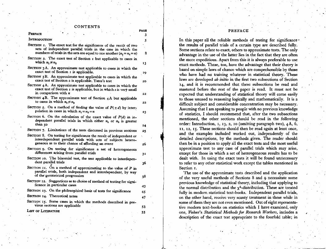
C O N T E N T S PAGE
PREFACE . 3
INTRODUCTION 5
SECTION 1. The exact test for the significance of the result of two sets of independent parallel trials in the case in which the numbers of trials in the sets are equal to one another (n1 = n2 = n) 8
SECTION 2. The exact test of Section I but applicable to cases in which n1 ≠ n2 13
SECTION 3 A. An approximate test applicable to cases in which the exact test of Section 1 is applicable. 19
SECTION 3 B. An approximate test applicable to cases in which the exact test of Section 2 is applicable. Yates's test 20
SECTION 4 A. An approximate test applicable to cases in which the exact test of Section 1 is applicable, but in which s is very small in comparison with n 22
SECTION 4B. The approximate test of Section 4A but applicable to cases in which n1 ≠ n2 22
SECTION 5. On a method of finding the value of P(±d) by inter-polation in cases in which n1 = n2 = n 23
SECTION 6. On the calculation of the exact value of P(d) in in-dependent parallel trials in which either n1 or n2 is greater than 50 24
SECTION 7. Limitations of the tests discussed in previous sections 25 SECTION 8. On testing for significance the result of independent or
interdependent parallel trials with sets of subjects hetero-geneous as to their chance of affording an event 26
SECTION 9. On testing for significance a set of heterogeneous differences arising from parallel trials 31
SECTION 10. The binomial test, the test applicable to interdepen-dent parallel trials 36
SECTION 11. On a method of approximating to the value of P in parallel trials, both independent and interdependent, by way of the geometrical progression 38
SECTION 12. Suggestions as to choice of method of testing for signi-ficance in particular cases 43
SECTION 13. On the philosophical basis of tests for significance 45 SECTION 14. Theoretical notes 47 SECTION 15. Some cases in which the methods described in pre-
vious sections are applicable 53 LIST OF LITERATURE 55
In this paper all the reliable methods of testing for significance the results of parallel trials of a certain type are described fully. Some sections relate to exact, others to approximate tests. The only advantage in the use of the latter lies in the fact that they are often the more expeditious. Apart from this it is always preferable to use exact methods. These, too, have the advantage that their theory is based on simple laws of chance which are comprehensible by those who have had no training whatever in statistical theory. These laws are developed ab initio in the first two subsections of Section 14, and it is recommended that these subsections be read and mastered before the rest of the paper is read. It must not be expected that understanding of statistical theory will come easily to those unused to reasoning logically and mathematically. It is a difficult subject and considerable concentration may be necessary. Assuming that I am speaking to people with no previous knowledge of statistics, I should recommend that, after the two subsections mentioned, the other sections should be read in the following order: Introduction, 1, 13, 2, 10 (omitting paragraph two), 4A, 6, 11, 12, 15. These sections should then be read again at least once, and the examples included worked out, independently of the detailed descriptions, by the methods given. The reader should then be in a position to apply all the exact tests and the most useful approximate test to any case of parallel trials which may arise, except for those in which a set of heterogeneous results has to be dealt with. In using the exact tests it will be found unnecessary to refer to any other statistical work except the tables mentioned in Section 1.
The use of the approximate tests described and the application of the very useful methods of Sections 8 and 9 necessitate some previous knowledge of statistical theory, including that applying to the normal distribution and the X2-distribution. These are treated fully in modern statistical text-books. Independent parallel trials, on the other hand, receive very scanty treatment in these while in some of them they are not even mentioned. Out of eight representative modern text-books on statistics which I have examined, only one, Fisher's Statistical Methods for Research Workers, includes a description of the exact test appropriate to the fourfold table; in
PREFACE
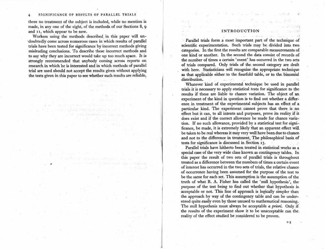
4 SIGNIFICANCE OF RESULTS OF PARALLEL TRIALS
three no treatment of the subject is included, while no mention is made, in any one of the eight, of the methods of our Sections 8, 9 and I, which appear to be new.
Workers using the methods described in this paper will un-doubtedly come across numerous cases in which results of parallel trials have been tested for significance by incorrect methods giving misleading conclusions. To describe these incorrect methods and to say why they are incorrect would take up too much space. I t is strongly recommended that anybody coming across reports on research in which he is interested and in which methods of parallel trial are used should not accept the results given without applying the tests given in this paper to see whether such results are reliable.
I N T R O D U C T I O N
Parallel trials form a most important part of the technique of scientific experimentation. Such trials may be divided into two; categories. In the first the results are comparable measurements of one kind or another. In the second the data consist of records of the number of times a certain 'event' has occurred in the two sets of trials compared. Only trials of the second category are dealt with here. Statisticians will recognize the appropriate technique as that applicable either to the fourfold table, or to the, binomial distribution.
Whatever kind of experimental technique be used in parallel trials it is necessary to apply statistical tests for significance to the results if these are liable to chance variation. The object of an experiment of the kind in question is to find out whether a differ-ence in treatment of the experimental subjects has an effect of a particular kind. The experiment cannot prove that there is no effect but it can, to all intents and purposes, prove its reality if it does exist and if the correct allowance be made for chance varia-tion. If no such allowance, provided by a statistical test for signi-ficance, be made, it is extremely likely that an apparent effect will be taken to be real whereas it may very well have been due to chance and not to the difference in treatment. The philosophical basis of tests for significance is discussed in Section 13.
Parallel trials have hitherto been treated in statistical works as a special case of the very wide class known as contingency tables. In this paper the result of two sets of parallel trials is throughout treated as a difference between the numbers of times a certain event of interest has occurred in the two sets of trials, the relative chance of occurrence having been assumed for the purpose of the test to be the same for each set. This assumption is the assumption of the truth of what R. A. Fisher has called the 'null hypothesis', the purpose of the test being to find out whether that hypothesis is acceptable or not. This line of approach is logically simpler than the approach by way of the contingency table and can be under-stood quite easily even by those unused to mathematical reasoning. The null hypothesis must always be acceptable a priori. Only if the results of the experiment show it to be unacceptable can the. reality of the effect studied be considered to be proven.
1-3
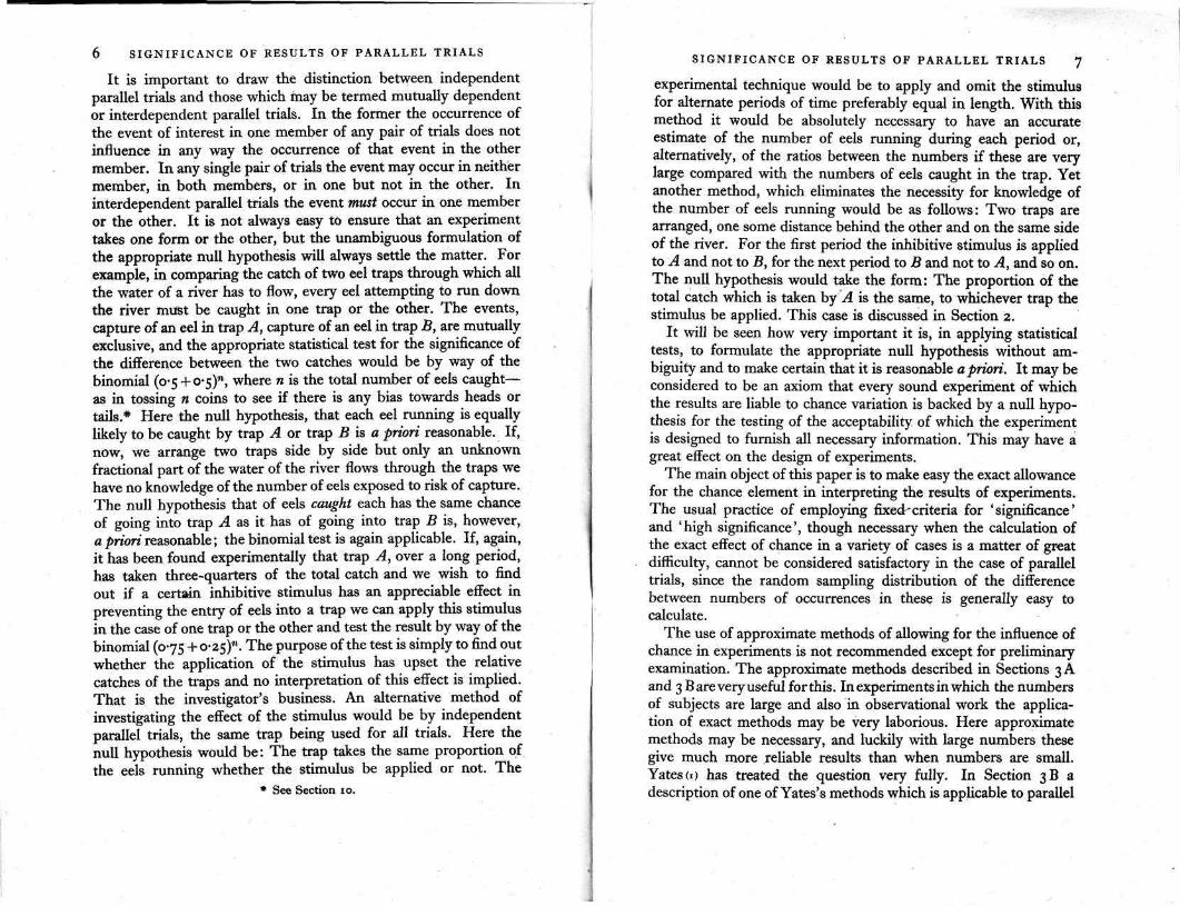
SIGNIFICANCE OF RESULTS OF PARALLEL TRIALS 7
experimental technique would be to apply and omit the stimulus for alternate periods of time preferably equal in length. With this method it would be absolutely necessary to have an accurate estimate of the number of eels running during each period or, alternatively, of the ratios between the numbers if these are very large compared with the numbers of eels caught in the trap. Yet another method, which eliminates the necessity for knowledge of the number of eels running would be as follows: Two traps are arranged, one some distance behind the other and on the same side of the river. For the first period the inhibitive stimulus is applied to A and not to B, for the next period to B and not to A, and so on. The null hypothesis would take the form: The proportion of the total catch which is taken by A is the same, to whichever trap the stimulus be applied. This case is discussed in Section 2.
It will be seen how very important it is, in applying statistical tests, to formulate the appropriate null hypothesis without am-biguity and to make certain that it is reasonable a priori. It may be considered to be an axiom that every sound experiment of which the results are liable to chance variation is backed by a null hypo-thesis for the testing of the acceptability of which the experiment is designed to furnish all necessary information. This may have a great effect on the design of experiments.
The main object of this paper is to make easy the exact allowance for the chance element in interpreting the results of experiments. The usual practice of employing fixed-criteria for 'significance' and 'high significance', though necessary when the calculation of the exact effect of chance in a variety of cases is a matter of great difficulty, cannot be considered satisfactory in the case of parallel trials, since the random sampling distribution of the difference between numbers of occurrences in these is generally easy to calculate.
The use of approximate methods of allowing for the influence of chance in experiments is not recommended except for preliminary examination. The approximate methods described in Sections 3A and 3B are very useful for this. In experiments in which the numbers of subjects are large and also in observational work the applica-tion of exact methods may be very laborious. Here approximate methods may be necessary, and luckily with large numbers these give much more reliable results than when numbers are small. Yates (1) has treated the question very fully. In Section 3B a description of one of Yates's methods which is applicable to parallel
6 SIGNIFICANCE OF RESULTS OF PARALLEL TRIALS
It is important to draw the distinction between independent parallel trials and those which may be termed mutually dependent or interdependent parallel trials. In the former the occurrence of the event of interest in one member of any pair of trials does not influence in any way the occurrence of that event in the other member. In any single pair of trials the event may occur in neither member, in both members, or in one but not in the other. In interdependent parallel trials the event must occur in one member or the other. It is not always easy to ensure that an experiment takes one form or the other, but the unambiguous formulation of the appropriate null hypothesis will always settle the matter. For example, in comparing the catch of two eel traps through which all the water of a river has to flow, every eel attempting to run down the river must be caught in one trap or the other. The events, capture of an eel in trap A, capture of an eel in trap B, are mutually exclusive, and the appropriate statistical test for the significance of the difference between the two catches would be by way of the binomial (0.5 + 0.5)n, where n is the total number of eels caught— as in tossing n coins to see if there is any bias towards heads or tails.* Here the null hypothesis, that each eel running is equally likely to be caught by trap A or trap B is a priori reasonable. If, now, we arrange two traps side by side but only an unknown fractional part of the water of the river flows through the traps we have no knowledge of the number of eels exposed to risk of capture. The null hypothesis that of eels caught each has the same chance of going into trap A as it has of going into trap B is, however, a priori reasonable; the binomial test is again applicable. If, again, it has been found experimentally that trap A, over a long period, has taken three-quarters of the total catch and we wish to find out if a certain inhibitive stimulus has an appreciable effect in preventing the entry of eels into a trap we can apply this stimulus in the case of one trap or the other and test the result by way of the binomial (0.75 + 0.25)n. The purpose of the test is simply to find out whether the application of the stimulus has upset the relative catches of the traps and no interpretation of this effect is implied. That is the investigator's business. An alternative method of investigating the effect of the stimulus would be by independent parallel trials, the same trap being used for all trials. Here the null hypothesis would be: The trap takes the same proportion of the eels running whether the stimulus be applied or not. The
* See Section 10.
8 S I G N I F I C A N C E OF RESULTS OF PARALLEL TRIALS
trials is given, and in Section 11 a method is described which is most useful and may perhaps be considered as superseding Yates's method.
In experimental work the case in which independent parallel trials are made with sets of subjects equal in number occurs much more often than that in which these differ in number. The former is here treated in detail, and tables are given from which the significance of a result can be estimated at a glance. These tables cover a con-siderable range of experimental numbers. A table is also provided by the aid of which the range of the exact test may be extended very easily, and it is thought that few cases will arise in laboratory experiments which are not covered by the tables. These have been very carefully checked, and are believed to be correct to within ±1 in the last figure. In Section 6 it is explained how to apply the exact test for significance in cases beyond the range of any of the tables.
All the tests described are applicable in a very wide field beyond that which may be strictly termed experimental. Some examples are given in Section 15.
SECTION I . The exact test for the significance of the result of two sets of independent parallel trials in the case in which the numbers of trials in the sets are equal to one another (n1 = n2 = n)
The appropriate technique is most easily presented by way of examples. Fortunately, experiments made at Wray Castle and other places by the F.B.A. provide examples suitable for the application of most of the necessary methods of statistical treatment. Though some of the actual figures obtained will be used, any necessary modifications will be made in the data to render them suitable for demonstration of statistical treatment.
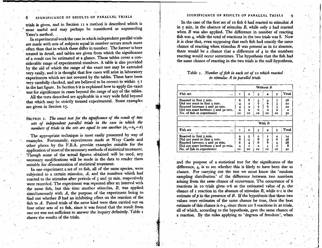
In one experiment a set of 10 fish, all of the same species, were subjected to a certain stimulus, A, and the numbers which had reacted to the stimulus after periods of 5 and 30 min. respectively were recorded. The experiment was repeated after an interval with the same fish, but this time another stimulus, B, was applied simultaneously with A, the purpose of the experiment being to find out whether B had an inhibiting effect on the reaction of the fish to A. Paired trials of the same kind were then carried out on four other sets of 10 fish, since it was found that the result from one set was not sufficient to answer the inquiry definitely. Table 1 shows the results of the trials.
and the purpose of a statistical test for the significance of the difference, 4, is to see whether this is likely to have been due to chance. For carrying out the test we must know the 'random sampling distribution' of the difference between two numbers arising from the same chance of occurrence. The occurrence of 6 reactions in 10 trials gives 0.6 as the estimated value of p, the chance of 1 reaction in the absence of stimulus B, while 0.2 is the estimate of p in the presence of B. If the hypothesis that these two values were estimates of the same chance be true, then the best estimate of this chance is 0.4, since there are 8 reactions in 20 trials, all of which, according to the hypothesis, gave the same chance of a reaction. By the rules applying to 'degrees of freedom', when
S I G N I F I C A N C E OF RESULTS OF PARALLEL TRIALS 9
In the case of the first set of 10 fish 6 had reacted to stimulus A in 5 min. in the absence of stimulus B, while only 2 had reacted when B was also applied. The difference in number of reacting fish was 4, while the total of reactions in the two trials was 8. Now it is clear that, even supposing that each fish had exactly the same chance of reacting when stimulus B was present as in its absence, there would be a chance that a difference of 4 in the numbers reacting would occur sometimes. The hypothesis that the fish had the same chance of reacting in the two trials is the null hypothesis,
Table 1. Number of fish in each set of 10 which reacted to stimulus A in parallel trials

10 SIGNIFICANCE OF RESULTS OF PARALLEL TRIALS
calculating the sampling distribution of differences between two numbers such as these, we restrict ourselves to numbers which give the same total, namely, 8. This is only common sense, for any pair of numbers giving a different total would give a different value for the hypothetical chance from that we have obtained. The distribution required is therefore that giving the probability of any given difference between two numbers of which the total is 8 and which have arisen by the same chance from 10 trials in each case. Such a probability may be written p(d), where d is the difference of which p is the probability. Since it is not justifiable a priori to assume that the difference is of particular sign, the probability considered is p( ± d).
It is clear that, as the number of trials is increased, the pro-bability of getting any particular difference becomes smaller and smaller since more and more differences become possible. Thus, in a statistical test, in order that all cases under test may be com-parable one with another, it is customary to consider, not p( ± d), the probability of + d, but P( ± d), the probability of a difference at least as great as d in either direction. The series to be used in the test therefore must give for each difference a term which is the sum of the probability of that difference and the probabilities of all possible greater differences. In other words P is the sum of the terms in the d-distribution beyond and including the terms p(+d), p(—d). The distribution has to answer, for each value of d, the question: Given 5 reactions and 2n — s non-reactions in 2n trials, what fraction of the total number of ways in which the reactions and non-reactions can be arranged in two sets of n in each gives the difference d reactions between the two sets? The calculation of this distribution is not difficult, but, since it varies both with variation in n the number of paired trials, and in s, the sum of the two numbers giving the difference d, it is not practicable to tabulate all distributions of the kind which may arise in experimental work. Distributions covering a fairly wide range of cases are tabulated in Tables 2, 3 and 4 of this paper. Table 2 applies to pairs of trials from 2 to 15 in number, while Tables 3 and 4 apply to trials of 20 and 30 pairs respectively. If it is desired therefore to make exact tests of the results of paired trials the number of these should at first be one of those included in the tables. Any really important effect would probably show up with trials of 30 or fewer pairs of subjects. In some cases, however, it will be necessary to increase the number of trials. Methods of dealing with these will be described later.
SIGNIFICANCE OF RESULTS OF PARALLEL TRIALS 11
Returning to our experimental result it is found, on reference to Table 2, that P( ± 4) = 0.169802, when n = 10 and s=8. A difference as great as 4 on either side would occur by chance about once in 6 trials if there were no difference between the chance of a reaction to A in the presence of B and that holding when B was absent. Clearly this is not sufficient to settle the question whether B has been proved to have an inhibitive effect. On repeating the experi-ment with another set of 10 fish it was found that the number of reactions was 5 with B against 8 without B. If we are justified in assuming that all the fish used in the experiments were homo-geneous as to their reactivity to A, we may add together the results of experiments and consider the combination as one experiment. If this be done, we now have a total number of paired trials, 20, and s=21, d=7. In Tables 2, 3 and 4 no value of s occurs greater than n, but P(d) when s=s is equal to P(d) when s=2n—s. Thus for entering Table 3, n = 20, s = 19, and P( + 7) is found to be equal to 0.05616. The generally employed criterion for significance is P=0.05. Where, however, an experiment can be repeated easily it is more important to notice whether or not P tends to decrease with increase in n rather than to adhere rigidly to a given value of P as a criterion. If there is a real difference between the chances of an occurrence in paired trials the value of P will always tend to decrease indefinitely as the number of trials is increased. If, on the other hand, there is no real difference between the chances, P will tend towards the value 0.5, varying in a random way about that value. Two values of P are not, however, sufficient to indicate a tendency. On further repetition of the experiment with another set of 10 fish, 3 reactions occurred without B against 2 with B. The value of n is now 30, 5=26, d=8. From Table 4 it is found that P=0.06729. This is rather greater than the corresponding value with n equal to 20, but such slight increases must be expected sometimes. The necessity for further trial is indicated. The next trial, taken in conjunction with those made previously, gave the values n = 40, s = 31,d=11. Since a value of 40 for n is beyond the range of the tables the value of P ( n ) must be calculated. Table 5 is included to facilitate this. We have to find the probability of a difference of 11 and of differences greater than 11 positive or nega-tive. The numbers, r, in Table 5 summing up to 31 and having differences of 11 or more are 21 and 10, 22 and 9, 23 and 8 and so on, the larger of any pair being equal to (s + d)/2. It will be seen that, when s is an odd number, only odd differences are possible.
12 SIGNIFICANCE OF RESULTS OF PARALLEL TRIALS
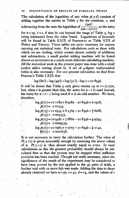
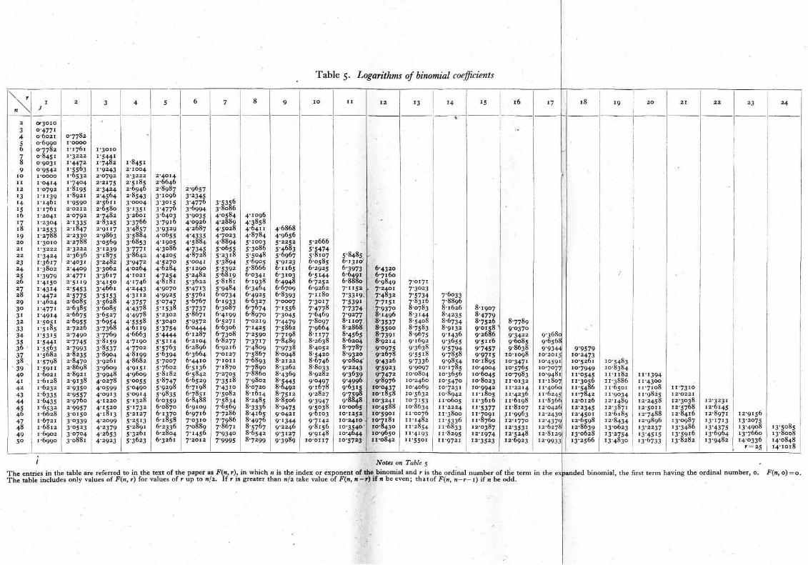
The calculation of the logarithm of any value consists of adding together the entries in Table 5 for the numbers, r, and
subtracting from the sum the logarithm of or the entry
for n = 2n, r=s, if that be not beyond the range of Table 5, log 2 being subtracted from the value found. Logarithms of factorials will be found in Table LXIX of Pearson (2) or Table XXX of Fisher and Yates (3). These tables are quite necessary for anyone carrying out statistical tests. For calculations such as those with which we are dealing, which consist almost entirely of additions and subtractions, a small pocket adding machine will be found almost as convenient as a much more elaborate calculating machine. All the numerical work in the present paper was done with a small pocket adder costing about 6s. A set of 4-figure mathematical tables is also necessary. For our present calculation we find from Pearson's Table LXIX that
It will be found that Table 5 only gives entries up to r=(1/2)n, but, when r is greater than this, the entry for n—r is used instead, the entry for n—r — 1 being used if n is an odd number. We have, therefore,
It is not necessary to carry the calculation further. The value of P( ± 11) is given accurately enough by summing the above values of p. P (±11) is thus almost exactly equal to 0.021. In such Calculations as this the greatest probability should always be cal-culated first so that the process may be stopped when sufficient precision has been reached. Though not really necessary, since the significance of the result of the experiment may be considered to have been proved by the test applied to the 40 pairs of trials, a further trial with 10 more fish was made. Adding the data to those already obtained we have n = 50, 5 = 42, d= 14, and the values of r

Table 2
Notes on Tables z, 3 and 4 When s is an odd number only odd differences are possible. When s is an even number only even differences are possible. The tables include values of P for values of s up to n. If s is greater than n take the value of 2n -s as the value of s for entering the tables. The figures in brackets in the tables give the number of ciphers preceding the first significant figure. Thus .0(4)411353 stands for .0000411353.

Tables 3 and 4. (n = 20), (n = 30)
Notes on Table 5
T h e entries in the table are referred to in the text of the paper as F(n, r), in which n is the index or exponent of the binomial and r is the ordinal number of the term in the expanded binomial, the first term having the ordinal number , 0. F(n, 0) = 0. T h e table includes only values of F(n, r) for values of r up to n/2. If r is greater than n/2 take value of F(n, n -r) if n be even; t h a t of F(n, n-r— 1) if n be odd.
Table 5. Logarithms of binomial coefficients
S I G N I F I C A N C E OF RESULTS OF PARALLEL TRIALS 13
are 28 and 14. For the subtrahend term in the necessary calcula-tion we have log (100!)—log (58!) — log (42!) — log 2, which is equal to 28.1501. Using the last row of entries in Table 5 and finding the value of p for differences from 14 to 22 inclusive it was found that the value of P(± 14) was approximately 0.0101. There is thus no reasonable doubt that the value of P tended to decrease as n was increased and that the reality of the difference 14 is proved, this implying that the stimulus B really had an inhibitive effect.
It must be emphasized that the 'significance' of a difference gives no estimate of the size or of the importance of the difference between two chances since the value of P depends so greatly on the number of trials. If for the present argument it is assumed that the tendency to react is the same in all of the fish, it must be assumed that the differences found are estimates of the same real difference, whether 10, 20, 30, 40 or 50 fish are used in the experiment. This difference has been shown to be real beyond all reasonable doubt by the test for significance. The value of the difference is best expressed by the ratio of one chance to the other. This ratio or fraction, B/not B, is variously estimated as 2/6, 7/14, 9/17, 10/21 and 14/28, according to the number of trials considered, and the chance of a reaction in the absence of B is fairly accurately esti-mated as twice the chance of a reaction in the presence of B.
If, in either member of a pair of n parallel trials, there are no occurrences, although a perfectly sound test for significance of an observed difference, d, may be made, yet no valid estimate of the ratio of chances is possible. If there are no occurrences it must not be assumed that there is really no chance of an occurrence. The chance should be assumed to be undetermined. A similar argument holds when one value of r is equal to n, for then there are no non-occurrences in one member. It is of no help to use the difference instead of the ratio and it may be very misleading.
SECTION 2. The exact test of Section 1 but applicable to cases in which n1 ≠n2
It is best, in experimental work employing parallel trials, when the experimental subjects are under control, to employ equal numbers of subjects in the members of each comparable set, since in that case an effect has equal chances of showing up, whether it be positive or negative. Such equality in numbers cannot always be obtained even in the laboratory and very rarely in field experiments.
1-7
14 S I G N I F I C A N C E OF RESULTS OF PARALLEL TRIALS
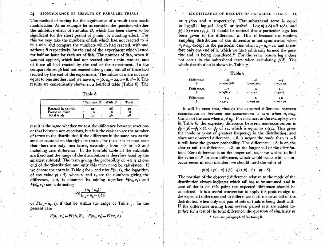
The method of testing for the significance of a result then needs modification. As an example let us consider the question whether the inhibitive effect of stimulus B, which has been shown to be significant for the short period of 5 min., is a lasting effect. For this we may take the numbers of fish which had. not reacted to A in 5 min. and compare the numbers which had reacted, with and without B respectively, by the end of the experiment which lasted for half an hour for each set of fish. The number of fish, when B was not applied, which had not reacted after 5 min. was 22, and of these all had reacted by the end of the experiment. In the comparable set 36 had not reacted after 5 min., but 28 of these had reacted by the end of the experiment. The values of n are not now equal to one another, and we have n1 = 36, n2 = 22, s=8, d=8. The results are conveniently shown in a fourfold table (Table 6). The
Table 6
result is the same whether we test the difference between reactions or that between non-reactions, but it is the easier to see the number of terms in the distribution if the difference in the same row as the smaller subtotal on the right be tested, for then it is at once seen that there are only nine terms, extending from —8 to + 8 and including zero difference. In the fourfold table all the subtotals are fixed and the range of the distribution is therefore fixed by the smallest subtotal. The term giving the probability of + 8 is at one end of the distribution and only this term need be calculated. If we denote the entry in Table 5 for n and r by F(n, r), the logarithm of any value p( + d), when r1 and r2 are the numbers giving the difference, + d, is obtained by adding together F(n1, r1) and F(n2, r2) and subtracting
or F(n1 + n2,s), if that be within the range of Table 5. In the present case
It will be seen that, though the expected difference between occurrences or between non-occurrences is zero when n1 = n2, this is not the case when n1≠n2. For instance, in the example given in Table 6, the expected difference between non-occurrences is 8/58x36 — 8/58x22 or 8/58 of 14, which is equal to 1.932. This gives the mode or point of greatest frequency in the distribution, and since our observed difference, + 8, is nearer the mode than is — 8 it will have the greater probability. The difference, + 8 , is on the shorter tail, the difference, — 8, on the longer tail of the distribu-tion. Zero difference is on the longer tail, so, if we wished to find the value of P for zero difference, which would occur with 4 non-occurrences in each member, we should need the value of
The position of the observed difference relative to the mode of the distribution always indicates which tail has to be summed, and in case of doubt on this point the expected difference should be calculated. It is a useful convention to apply the positive sign to the expected difference and to differences on the shorter tail of the distribution when only one pair of sets of trials is being dealt with. If the differences arising from several paired sets are added to-gether for a test of the total difference, the question of similarity or
* See last paragraph of Section 3 B.
Table 7
S I G N I F I C A N C E OF RESULTS OF PARALLEL TRIALS 15
or 7.4809 and 0 respectively. T h e subtrahend term is equal to log 58! - l o g 50! - l o g 8! or 9.2826. Logp(+ 8) = 2.1983 and p( + 8) = 0.01579. It should be noticed that a particular sign has been given to the difference, d. This is because the random sampling distribution of the difference is not symmetrical when n1 ≠ n2, except in the particular case when n1 + n2 = 2S, and there-fore only one end of it, which we have arbitrarily termed the posi-tive end, is being considered.* For the same reason log 2 does not occur in the subtrahend term when calculating p(d). The whole distribution is shown in Table 7.
SIGNIFICANCE OF RESULTS OF PARALLEL TRIALS 17
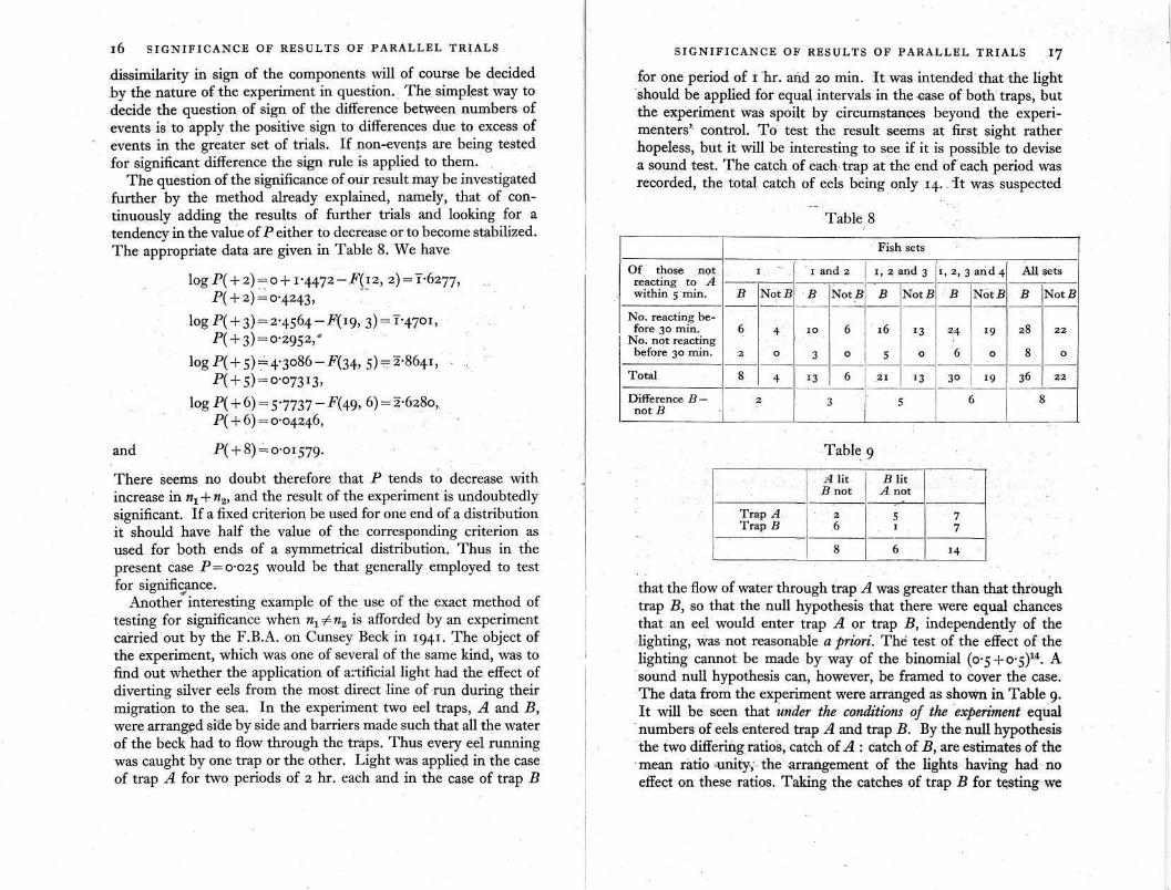
for one period of 1 hr. and 20 min. It was intended that the light should be applied for equal intervals in the case of both traps, but the experiment was spoilt by circumstances beyond the experi-menters' control. To test the result seems at first sight rather hopeless, but it will be interesting to see if it is possible to devise a sound test. The catch of each trap at the end of each period was recorded, the total catch of eels being only 14. It was suspected
Table 8
Table 9
that the flow of water through trap A was greater than that through trap B, so that the null hypothesis that there were equal chances that an eel would enter trap A or trap B, independently of the lighting, was not reasonable a priori. The test of the effect of the lighting cannot be made by way of the binomial (0.5+0.5)14. A sound null hypothesis can, however, be framed to cover the case. The data from the experiment were arranged as shown in Table 9. It will be seen that under the conditions of the experiment equal numbers of eels entered trap A and trap B. By the null hypothesis the two differing ratios, catch of A : catch of B, are estimates of the mean ratio unity, the arrangement of the lights having had no effect on these ratios. Taking the catches of trap B for testing we
There seems no doubt therefore that P tends to decrease with increase in n1 + n2, and the result of the experiment is undoubtedly significant. If a fixed criterion be used for one end of a distribution it should have half the value of the corresponding criterion as used for both ends of a symmetrical distribution. Thus in the present case P = 0.025 would be that generally employed to test for significance.
Another interesting example of the use of the exact method of testing for significance when n1≠n2 is afforded by an experiment carried out by the F.B.A. on Cunsey Beck in 1941. The object of the experiment, which was one of several of the same kind, was to find out whether the application of artificial light had the effect of diverting silver eels from the most direct line of run during their migration to the sea. In the experiment two eel traps, A and B, were arranged side by side and barriers made such that all the water of the beck had to flow through the traps. Thus every eel running was caught by one trap or the other. Light was applied in the case of trap A for two periods of 2 hr. each and in the case of trap B
and
l6 SIGNIFICANCE OF RESULTS OF PARALLEL TRIALS
dissimilarity in sign of the components will of course be decided by the nature of the experiment in question. The simplest way to decide the question of sign of the difference between numbers of events is to apply the positive sign to differences due to excess of events in the greater set of trials. If non-events are being tested for significant difference the sign rule is applied to them.
The question of the significance of our result may be investigated further by the method already explained, namely, that of con-tinuously adding the results of further trials and looking for a tendency in the value of P either to decrease or to become stabilized. The appropriate data are given in Table 8. We have
SIGNIFICANCE OF RESULTS OF PARALLEL TRIALS 19
SECTION 3 A. An approximate test applicable to cases in which the exact test of Section 1 is applicable
The standard deviation of the difference between two numbers distributed binomially may be expected, from analogy with the normal distribution, to be approximately equal to √2 times that of either component. These, by the null hypothesis, having been assumed to be samples of n from the binomial distribution,
, and each therefore having a standard deviation
equal t o , the standard deviation of the difference between
them may be expected to be approximately equal to
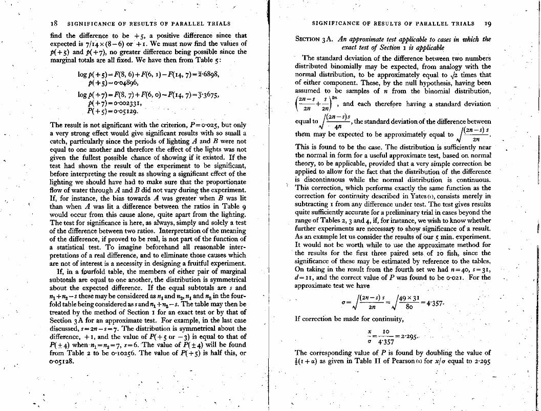
This is found to be the case. The distribution is sufficiently near the normal in form for a useful approximate test, based on normal theory, to be applicable, provided that a very simple correction be applied to allow for the fact that the distribution of the difference is discontinuous while the normal distribution is continuous. This correction, which performs exactly the same function as the correction for continuity described in Yates (1), consists merely in subtracting 1 from any difference under test. The test gives results quite sufficiently accurate for a preliminary trial in cases beyond the range of Tables 2, 3 and 4, if, for instance, we wish to know whether further experiments are necessary to show significance of a result. As an example let us consider the results of our 5 min. experiment. It would not be worth while to use the approximate method for the results for the first three paired sets of 10 fish, since the significance of these may be estimated by reference to the tables. On taking in the result from the fourth set we had n = 40, s = 31, d=11, and the correct value of P was found to be 0.021. For the approximate test we have
If correction be made for continuity,
The corresponding value of P is found by doubling the value of 1/2(1 + a) as given in Table II of Pearson (2) for x/σ equal to 2.295
The result is not significant with the criterion, P=0.025, but only a very strong effect would give significant results with so small a catch, particularly since the periods of lighting A and B were not equal to one another and therefore the effect of the lights was not given the fullest possible chance of showing if it existed. If the test had shown the result of the experiment to be significant, before interpreting the result as showing a significant effect of the lighting we should have had to make sure that the proportionate flow of water through A and B did not vary during the experiment. If, for instance, the bias towards A was greater when B was lit than when A was lit a difference between the ratios in Table 9 would occur from this cause alone, quite apart from the lighting. The test for significance is here, as always, simply and solely a test of the difference between two ratios. Interpretation of the meaning of the difference, if proved to be real, is not part of the function of a statistical test. To imagine beforehand all reasonable inter-pretations of a real difference, and to eliminate those causes which are not of interest is a necessity in designing a fruitful experiment.
If, in a fourfold table, the members of either pair of marginal subtotals are equal to one another, the distribution is symmetrical about the expected difference. If the equal subtotals are s and n1+n2-s these may be considered as n1 and n2, n1 and n2 in the four-fold table being considered as s and n1+n2—s. The table may then be treated by the method of Section 1 for an exact test or by that of Section 3A for an approximate test. For example, in the last case discussed, s=2n — s=7. The distribution is symmetrical about the difference, + 1 , and the value of P( + 5 or —3) is equal to that of P( ± 4) when n1=n2 = 7, s=6. The value of P ( ± 4 ) will be found from Table 2 to be 0.10256. The value of P(+5) is half this, or 0.05128.
l 8 SIGNIFICANCE OF RESULTS OF PARALLEL TRIALS
find the difference to be + 5 , a positive difference since that expected is 7/14 x (8 — 6) or +1. We must now find the values of p( + 5) and p( + 7), no greater difference being possible since the marginal totals are all fixed. We have then from Table 5:
20 SIGNIFICANCE OF RESULTS OF PARALLEL TRIALS
and subtracting this from 2. P is found to be equal to 0.022 to two significant figures, an extremely good approximation. Taking in the result from the fifth pair we have
Significance of the result is thus somewhat overestimated by the approximate method since the true value of P is 0.0101. As it is not possible to say beforehand whether significance will be over-estimated or underestimated by the approximate method, it is preferable to use the exact method in published papers when time allows. It cannot be considered satisfactory to publish figures which are known to be wrong even if the errors are not likely to be large.
A method of interpolation is described, in a later section, which is useful for obtaining quickly a value of P very near to the true value in certain cases.
SECTION 3B. An approximate test applicable to cases in which the exact test of Section 2 is applicable. Yates's test
The simplest way to apply Yates's test for those who have got used to the methods of the previous sections is as follows. The example of Table 6 will serve as an illustration.
Denote by n the smallest of the four marginal subtotals. This may be either in the pair on the right or in the pair at the bottom. Whichever pair it occurs in, denote by n' the smaller of the other pair.
Denote by N the sum of either pair of subtotals. Denote by m the smallest expected value in the body of the table.
This is equal to nn'/N. Denote by p the value of m/n. Proceed as follows for the example
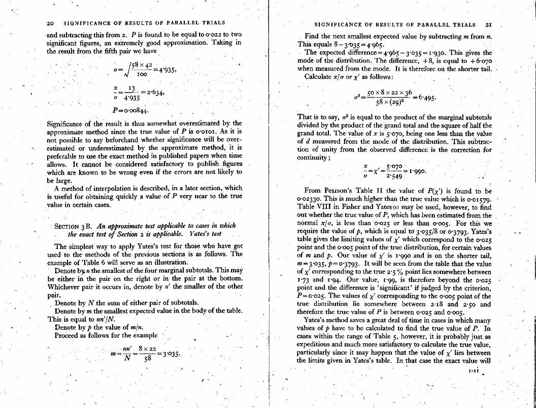
From Pearson's Table II the value of P(x) is found to be 0.02330. This is much higher than the true value which is 0.01579. Table VIII in Fisher and Yates (3) may be used, however, to find out whether the true value of P, which has been estimated from the normal x/σ, is less than 0.025 or less than 0.005. For this we require the value of p, which is equal to 3.035/8 or 0.3793. Yates's table gives the limiting values of x' which correspond to the 0.025 point and the 0.005 point of the true distribution, for certain values of m and p. Our value of x' is 1.990 and is on the shorter tail, m = 3.035,p=0.3793. It will be seen from the table that the value of x' corresponding to the true 2.5 % point lies somewhere between 1.73 and 1.94. Our value, 1.99, is therefore beyond the 0.025 point and the difference is 'significant' if judged by the criterion, P= 0.025. The values of x' corresponding to the 0.005 point of the true distribution lie somewhere between 2.18 and 2.50 and therefore the true value of P is between 0.025 and 0.005.
Yates's method saves a great deal of time in cases in which many values of p have to be calculated to find the true value of P. In cases within the range of Table 5, however, it is probably just as expeditious and much more satisfactory to calculate the true value, particularly since it may happen that the value of x' lies between the limits given in Yates's table. In that case the exact value will
I-II
That is to say, σ2 is equal to the product of the marginal subtotals divided by the product of the grand total and the square of half the grand total. The value of x is 5.070, being one less than the value of d measured from the mode of the distribution. This subtrac-tion of unity from the observed difference is the correction for continuity;
SIGNIFICANCE OF RESULTS OF PARALLEL TRIALS 21
Find the next smallest expected value by subtracting m from n. This equals 8 —3.035=4.965.
The expected difference = 4.965 —3.035 = 1.930. This gives the mode of the distribution. The difference, + 8, is equal to + 6.070 when measured from the mode. It is therefore on the shorter tail.
Calculate x/σ or x' as follows:
2 2 S I G N I F I C A N C E OF RESULTS OF PARALLEL TRIALS
have to be calculated. Instead of applying Yates's method in cases beyond the range of Table 5 it is preferable to use the method of Section 11 since in most cases this will settle the question of significance.
SECTION 4A. An approximate test applicable to cases in which the exact test of Section 1 is applicable, but in which s is very small in comparison with n If n, the number of paired trials, is at least 30 times as great as s,
the distribution of the difference, d, is expressed closely enough by the binomial (0.5 + 0.5)8. Thus, if the number of reactions to stimulus A in the presence of B be 2, when 300 fish are used in the experiment, the number of reactions in the absence of B being 8, the chance of the difference, + 6, is given approximately by the binomial term 10C2 (0.5)10. The chance of the difference, ± 6, is twice this, that is to say, the index is s— 1 or 9 instead of 10. To obtain the value of P(± 6) the terms nearer the tails of the dis-tribution must be added to the term for r = 2. The values of the terms to be summed may be obtained quickly from Table 5 when s lies between 2 and 50 inclusive.* In the present case the antilogs of the entries for n=10, r = 2, 1, 0, are summed and the sum divided by 29 to give P(±6). Its value is found to be 0.1093. The method is approximate and only gives exact results when n=∞. The true value of P( ± 6), when n — 300, s = 10, is equal to 0.1064. The true value of P( ± 8) is 0.020466, the binomial approximation 0.02148 and the corresponding values of P( ± 10) are 0.0018096 and 0.00195 respectively. The binomial approximations rapidly approach the true values as n/s is increased, but even when this is only equal to 30 the binomial approximations are nearer the true values than are those given by the methods of Section 3A.
SECTION 4B. The approximate test of Section 4A but applicable to cases in which n1≠n2
If the numbers of subjects in a set of parallel trials are both very large in comparison with 5 but not equal to one another the dis-tribution of the difference, d, is not that of the binomial (0.5 +0.5)s
but that of the binomial (q +p)s, in which
* For treatment of cases beyond the range of Table 5, see Sections 10 and 11.
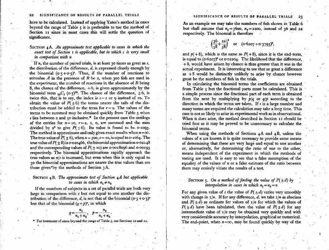
and p(+ 8), which is the same as P( + 8), since it is the end-term, is equal to (0.6207)8 or 0.02204. The likelihood that the difference, + 8, would have arisen by chance is thus greater than it was in the actual experiment. It is interesting to see that so great a difference as + 8 would be distinctly unlikely to arise by chance however great be the numbers of fish in the trials.
In calculating the binomial terms the coefficients are obtained from Table 5 but the fractional parts must be calculated. This is a simple process since the fractional part of each term is obtained from the next by multiplying by p/q or q/p according to the direction in which the terms are taken. If s is a large number and many terms are required the calculation may take a long time. This case is not so likely to arise in experimental work as in observational. When it does arise, the method described in Section 11 should be tried first as it may be proved to be unnecessary to calculate the binomial terms.
When using the methods of Sections 4A and 4B, unless the values of n are known it is quite necessary to provide some means of determining that these are very large and equal to one another or, alternatively, for determining the ratio of one to the other, means independent of the experiment in which the methods of testing are used. It is easy to see that a false assumption of the equality of the values of n or a false estimate of the ratio between them may entirely vitiate the results of a test.
SECTION 5. On a method of finding the value of P( ± d) by interpolation in cases in which n1 = n2 = n
For any given value of 5 the value of P( ± d) varies very smoothly with change in 1/n. If for any difference, d, we take 1/n as abscissa and P(±d) as ordinate for values of 1/n for which the values of P(±d) have been tabulated, then the value of P(±d) for any intermediate value of 1/n may be obtained very quickly and with very considerable accuracy by interpolation, graphical or numerical. The end-point, when n=00, may be found quickly by way of the
S I G N I F I C A N C E OF RESULTS OF PARALLEL TRIALS 2 3
As an example we may take the numbers of fish shown in Table 6 but shall assume that n1 = 3600, n2 = 2200, instead of 36 and 22 respectively. The binomial is therefore
SIGNIFICANCE OF RESULTS OF PARALLEL TRIALS 25
The most convenient form of the equation for calculating p in cases beyond the range of Table 5 is that given by Yates (1). This gives the following rule.
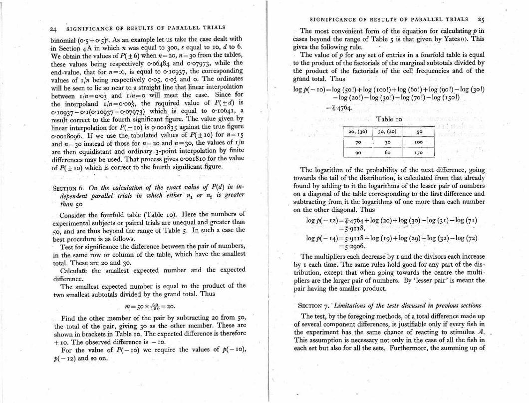
The value of p for any set of entries in a fourfold table is equal to the product of the factorials of the marginal subtotals divided by the product of the factorials of the cell frequencies and of the grand total. Thus
The logarithm of the probability of the next difference, going towards the tail of the distribution, is calculated from that already found by adding to it the logarithms of the lesser pair of numbers on a diagonal of the table corresponding to the first difference and subtracting from it the logarithms of one more than each number on the other diagonal. Thus
The multipliers each decrease by 1 and the divisors each increase by 1 each time. The same rules hold good for any part of the dis-tribution, except that when going towards the centre the multi-pliers are the larger pair of numbers. By 'lesser pair' is meant the pair having the smaller product.
SECTION 7. Limitations of the tests discussed in previous sections The test, by the foregoing methods, of a total difference made up
of several component differences, is justifiable only if every fish in the experiment has the same chance of reacting to stimulus A. This assumption is necessary not only in the case of all the fish in each set but also for all the sets. Furthermore, the summing up of
Find the other member of the pair by subtracting 20 from 50, the total of the pair, giving 30 as the other member. These are shown in brackets in Table 10. The expected difference is therefore + 10. The observed difference is — 10.
For the value of P ( - 1 0 ) we require the values of p(-10), p( — 12) and so on.
24 SIGNIFICANCE OF RESULTS OF PARALLEL TRIALS
binomial (0.5 + 0.5)s. As an example let us take the case dealt with in Section 4A in which n was equal to 300, s equal to 10, d to 6. We obtain the values of P( ± 6) when n = 20, n = 30 from the tables, these values being respectively 0.06484 and 0.07973, while the end-value, that for n=∞, is equal to 0.10937, the corresponding values of \\n being respectively 0.05, 0.03 and 0. The ordinates will be seen to lie so near to a straight line that linear interpolation between 1/N = 0.03 and 1/n = 0 will meet the case. Since for the interpoland 1/n = 0.003, the required value of P(±d) is 0.10937—0.1(0.10937 — 0.07973) which is equal to 0.10641, a result correct to the fourth significant figure. The value given by linear interpolation for P(± 10) is 0.001835 against the true figure 0.0018096. If we use the, tabulated values of P(± 10) for n=15 and n = 30 instead of those for n = 20 and n = 30, the values of 1/n are then equidistant and ordinary 3-point interpolation by finite differences may be used. That process gives 0.001810 for the value of P( ± 10) which is correct to the fourth significant figure.
SECTION 6. On the calculation of the exact value of P (d) in in-dependent parallel trials in which either n1 or n2 is greater than 50 Consider the fourfold table (Table 10). Here the numbers of
experimental subjects or paired trials are unequal and greater than 50, and are thus beyond the range of Table 5. In such a case the best procedure is as follows.
Test for significance the difference between the pair of numbers, in the same row or column of the table, which have the smallest total. These are 20 and 30.
Calculate the smallest expected number and the expected difference.
The smallest expected number is equal to the product of the two smallest subtotals divided by the grand total. Thus

26 SIGNIFICANCE OF RESULTS OF PARALLEL TRIALS
the various differences implies that, should their sum prove to be significant, the effect producing each difference is throughout of the same kind. If this be not so the result of adding the differences together, each with its particular sign, is meaningless. Hetero-geneity among the experimental subjects may render the test of a total difference unsound, since it is implied in the null hypothesis that all fish have the same chance of reacting to stimulus A and therefore that hypothesis is unreasonable a priori if it is known that the chance varies. Since all the subjects in any set will almost certainly have been treated as far as possible in exactly the same way and will have been chosen with an eye to homogeneity it is probably reasonable to assume that there is no significant heterogeneity among the subjects in any set. If there is doubt whether there is homo-geneity between the sets it is a simple matter to test whether it is reasonable to assume this. The test is fully described in Section 21 of Fisher (4), and it is therefore unnecessary to give an account of it here. In applying the test s in each set corresponds to a in Fisher (p. 90), 2n — s to a', total x to n, total 2n — s to n'. If heterogeneity be found it is preferable to use the methods of the next section.
The methods of Sections 8 and 9 do not give reliable results except when, in the case of independent parallel trials, n 1 =n 2 in each component distribution and when, in interdependent parallel trials, each component is of the form, (0.5+0.5)n.
SECTION 8. On testing for significance the result of independent or interdependent parallel trials with sets of subjects heterogeneous as to their chance of affording an event
If the members of a set of differences be additive in nature owing to their investigated cause being the same throughout, but if the sets of experimental subjects be heterogeneous as to the variate in which differences are measured for statistical testing, the null hypothesis takes a form rather different from that applying to homogeneous variation in that variate. We have to consider a series of independent hypotheses each having the form: The difference is really zero and any difference arising from random sampling is equally likely to be positive or negative; but it is not implied that all the component differences have the same random sampling distribution. To make one comprehensive test which is applicable to such a case each observed difference must be given its sign and each must be graded according to the probability that
The value of p(d) is preferably taken as the difference between the tabulated values of ½(1 + α) corresponding to the values of z taken from Pearson's Table II . This process renders it unnecessary to interpolate between tabulated values of z. We have therefore
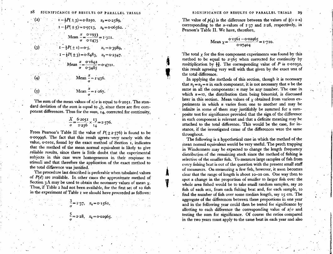
Taking the nearest tabulated value of ½(1 + α) in that table, the corresponding value of z is found to be 0.1561:
where zd and Z(d+2) are respectively the normal ordinates at the inner and outer ends of the probability interval p(d) in the normal distribution. The entries in Tables 2, 3 and 4 are the values of P( ± d). For the example used in the previous method the procedure is as follows, using the values of P given in Table 2 for n = 10:
SIGNIFICANCE OF RESULTS OF PARALLEL TRIALS 27
a difference at least as great will arise by chance if the null hypo-thesis be true. The only practicable way of grading them according to the value of P in each case is to put them On the 'normal scale', that is to say, to allot to each of them the value of x/σ, in the normal distribution, which gives the same value of P. The values of x/σ, each with its appropriate sign, may then be summed for a composite test of the truth of all the null hypotheses. Though the distribution of this sum is not exactly normal in form yet it rapidly approaches that form as the number of values in the sum is increased. To correct for continuity the total X/σ is multiplied by (D — 1)/D, where D is the total difference.
According to the most accurate method the value of X/σ for an aggregate difference is calculated from the true values of P and p for each of the component differences. What is found for each is the mean normal equivalent abscissa, x/σ, for the probability interval, p, corresponding to each difference. It may be shown that, for any difference, d, with particular sign,
From Pearson's Table II the value of P( ± 2.576) is found to be 0.009996. The fact that this result agrees very nearly with the value, 0.0101, found by the exact method of Section 1, indicates that the method of the mean normal equivalent is likely to give reliable results, since there is little doubt that the experimental subjects in this case were homogeneous in their response to stimuli and that therefore the application of the exact method to the total difference was justified.
The procedure last described is preferable when tabulated values of P(d) are available. In other cases the approximate method of Section 3 A may be used to obtain the necessary values of mean x. Thus, if Table 2 had not been available, for the first set of 10 fish in the experiment of Table 1 we should have proceeded as follows:
The sum of the mean values of x/σ is equal to 6.2051. The stan-dard deviation of the sum is equal to √5, since there are five com-ponent differences. Thus for the sum, 14, corrected for continuity,
28 SIGNIFICANCE OF RESULTS OF PARALLEL TRIALS SIGNIFICANCE OF RESULTS OF PARALLEL TRIALS 29
The value of p(4) is the difference between the values of ½(1 + α) corresponding to the x-values of 1.37 and 2.28, respectively, in Pearson's Table II . We have, therefore,
The total x for the five component experiments was found by this method to be equal to 2.565 when corrected for continuity by multiplication by 13/14. The corresponding value of P is 0.01032, this result agreeing very well with that given by the exact test of the total difference.
In applying the methods of this section, though it is necessary that n 1 =n 2 = n in each component, it is not necessary that n be the same in all the components: n may be any number. The case in which n=∞, the distribution then being binomial, is discussed later in this section. Mean values of x obtained from various ex-periments in which n varies from one to another and may be infinite in some of them may justifiably be summed for a com-posite test for significance provided that the sign of the difference in each component is relevant and that a definite meaning may be attached to the total difference. This would be the case, for in-stance, if the investigated cause of the differences were the same throughout.
The following is a hypothetical case in which the method of the mean normal equivalent would be very useful. The perch trapping in Windermere may be expected to change the length frequency distribution of the remaining stock since the method of fishing is selective of the smaller fish. To measure large samples of fish from every fishing beat is out of the question with the present small staff of measurers. On measuring a few fish, however, it soon becomes clear that the range of length is about 10-20 cm. One way then to spot a change in the proportion of smaller to larger fish over the whole area fished would be to take small random samples, say 20 fish of each sex, from each fishing beat and, for each sample, to find the number of fish over some median length, say 15 cm. The aggregate of the differences between these proportions in one year and in the following year could then be tested for significance by allotting to each difference the corresponding value of x/σ and testing the sum for significance. Of course the ratios compared in the two years must apply to the same beat in each year and also

SIGNIFICANCE OF RESULTS OF PARALLEL TRIALS 31
equal samples if these samples form a very small proportion of the sampled field. In this case, as is explained in Section 14(3), the distribution of the difference between the numbers in any pair of samples is expressed by the binomial (0.5 + 0.5)8, where s is the total number of occurrences in the two samples. For example, let us suppose that a farmer who is also a statistician wishes to find out whether infestation of a particular piece of land by wireworms has increased or decreased significantly from one year to the next. In the first year he takes a bucketful of soil from each of ten different sites on the land and counts the wireworms in each bucketful. On some sites, however, he finds that he has to take two bucketfuls to obtain any wireworms. In the next year he repeats the process on the same sites, taking of course the same number of bucketfuls of soil as he did on the same site the year before. The test for sig-nificance of the change in infestation is the same as in our previous example, in each component experiment the difference between numbers of wireworms being considered as a term of the binomial (0.5 +0.5)8, in which s is the total number counted at the same site in the two years.
The test just explained is applicable in a very wide field. Here are some examples: (1) comparing the catch of perch traps in different years over large areas; (2) comparing the catch of plank-tonic organisms from a large number of different places or periods; (3) uniformity trials, pairs being chosen at random from a large number of experimental takings extending over the period or the area for which the question of uniformity in distribution of organisms or other subjects is of interest.
SECTION 9. On testing for significance a set of heterogeneous differences arising from parallel trials
Sometimes it may be of interest to test for significance the aggregate of a series of differences of which the sign is not taken into account. For example, an experiment similar to that discussed in Section 1 might be made in which, however, the fish in each set of 10 were of species different from those in the other sets. Here the question of interest might be whether the application of stimulus B caused a change in the reaction of the fish to A, whether or not the change was in the same sense in each case. The question would be, therefore, whether the aggregate of such differences as were observed, without regard to sign, in the proportion reacting to A,
The values of mean x are summed, multiplied by 17/18 to correct for con-tinuity, and the result divided by √4 or 2, the value of P for total x being obtained from Pearson's Table II as in our previous example.
The method of mean x is also applicable to testing for signi-ficance of differences between numbers of occurrences in paired
30 SIGNIFICANCE OF RESULTS OF PARALLEL TRIALS
approximately to the same date. Changes in sex ratio could be investigated in a similar way. In this kind of work it would save a great deal of time if the number of fish in each sample were one of the values of n included in our tables.
The methods of this section are also applicable to testing for significance a series of differences between numbers of occur-rences in interdependent parallel trials in cases in which the chance of an occurrence varies widely from set to set of trials. For instance, in a series of experiments to find out whether a line of lights has a diverting effect on migrating eels, experiments in which all migrating eels are caught in one or other of two traps, A and B, it may be found that the proportion of eels caught in trap A varies widely. It would not, in this case, be justifiable to add together all the numbers of eels caught in trap A and then to test the ratio between that total and the total caught in trap B by way of the binomial (0.5 + 0.5)n. It would be preferable, in each component experiment, to find the mean value of x/σ or x corresponding to each difference between A and B, and to test the total x for signi-ficance. It is just as simple a matter to find the required values of X in a case of this kind as it was in our previous example. Let us suppose, for instance, that in four experiments the numbers of eels in trap A and in trap B were, respectively, 1,5; 4, 9; 3 , 2 ; 5 , 15. By the method explained in Section 10 the values of P (±4) , P( ± 5), P( ± 1), and P( ± 10) are found to be, respectively, 0.2188, 0.2669, 1 and 0.04139, while the corresponding values of P(d+2) are, respectively, 0.03125, 0.09018, 0.375 and 0.01179. The value of p( + 4) is equal to ½(0.2188-0.03125) or 0.09377. The required values of p will have been found, however, during the process of calculating those of P. For the first difference we have, therefore,
SIGNIFICANCE OF RESULTS OF PARALLEL TRIALS 33
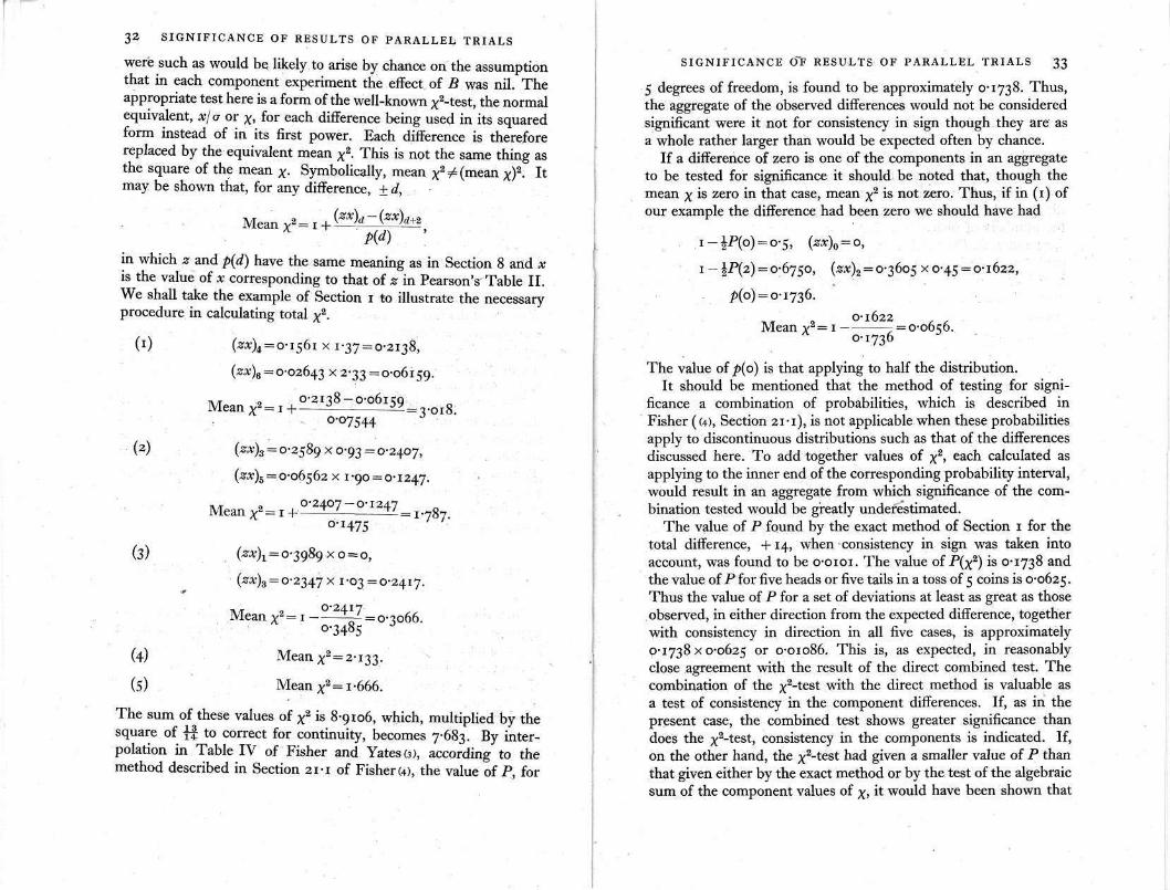
5 degrees of freedom, is found to be approximately 0.1738. Thus, the aggregate of the observed differences would not be considered significant were it not for consistency in sign though they are as a whole rather larger than would be expected often by chance.
If a difference of zero is one of the components in an aggregate to be tested for significance it should be noted that, though the mean x is zero in that case, mean x2 is not zero. Thus, if in (1) of our example the difference had been zero we should have had
The value of p(o) is that applying to half the distribution. It should be mentioned that the method of testing for signi-
ficance a combination of probabilities, which is described in Fisher ((4), Section 21.1), is not applicable when these probabilities apply to discontinuous distributions such as that of the differences discussed here. To add together values of x2, each calculated as applying to the inner end of the corresponding probability interval, would result in an aggregate from which significance of the com-bination tested would be greatly underestimated.
The value of P found by the exact method of Section 1 for the total difference, +14, when consistency in sign was taken into account, was found to be 0.0101. The value of P(x2) is 0.1738 and the value of P for five heads or five tails in a toss of 5 coins is 0.0625. Thus the value of P for a set of deviations at least as great as those observed, in either direction from the expected difference, together with consistency in direction in all five cases, is approximately 0.1738x0.0625 or 0.01086. This is, as expected, in reasonably close agreement with the result of the direct combined test. The combination of the x2-test with the direct method is valuable as a test of consistency in the component differences. If, as in the present case, the combined test shows greater significance than does the x2-test, consistency in the components is indicated. If, on the other hand, the x2-test had given a smaller value of P than that given either by the exact method or by the test of the algebraic sum of the component values of x, it would have been shown that
The sum of these values of x2 is 8.9106, which, multiplied by the square of 13/14 to correct for continuity, becomes 7.683. By inter-polation in Table IV of Fisher and Yates (3), according to the method described in Section 21-1 of Fisher (4), the value of P, for
in which z and p(d) have the same meaning as in Section 8 and x is the value of x corresponding to that of z in Pearson's Table II . We shall take the example of Section 1 to illustrate the necessary procedure in calculating total x2.
32 SIGNIFICANCE OF RESULTS OF PARALLEL TRIALS
were such as would be likely to arise by chance on the assumption that in each component experiment the effect of B was nil. The appropriate test here is a form of the well-known x2-test, the normal equivalent, x/σ or x, for each difference being used in its squared form instead of in its first power. Each difference is therefore replaced by the equivalent mean x2. This is not the same thing as the square of the mean X. Symbolically, mean x2≠(mean x)2. It may be shown that, for any difference, ± d,

34 SIGNIFICANCE OF RESULTS OF PARALLEL TRIALS
the sum of the differences was an aggregate of inconsistent differ-ences. The sets of experimental subjects would have varied more than would be expected by chance in their response to the causes of the differences.
An interesting example of the application of the methods of the present section is a test of consistency in the catches of floating fish eggs made by parallel vertical hauls with a plankton net at different places and times. In a short series of such pairs of hauls the numbers of plaice eggs caught were, respectively, 2, 4; 5, 1; 6, 7; and 3, 6. The total number of plaice eggs caught in the first-made hauls of each pair was 16 and in the second hauls 18, so that it is clear that in this case there was no significant tendency for the catch of first hauls to be greater than that of second hauls or vice versa. A test for significance of total x is not called for. It is of interest, however, to find out whether there is, on the whole, significant discrepancy between the catches of first and those of second hauls. The x2-test is applicable. For the first pair we have
For the other three pairs the values of mean x2 are, respectively, 2.548, 0.0997 and 0.9707. The sum of these values is 4.2646, which, multiplied by the square of 9/10, becomes 3.453. From Table IV of Fisher and Yates (3) the value of P, for 4 degrees of freedom, is found to lie between 0.3 and 0.5. Thus no significant discrepancy is shown between the catches of first and second hauls of the net at each place. The data were, however, taken from a long series of similar data, and it must not be concluded that such discrepancy would not have been shown had all the data been included in the test. If, after examination of all the relevant data, it were to be found that there was no significant discrepancy between the catches of first and second hauls it would be shown to be reasonable to assume not only that the catching power of the net was uniform but also that variation in the quantity of the eggs under a given surface of water between the first and second hauls of each pair was only such as could be ascribed to pure chance.
in which S stands for 'the sum of. P(x2) is found from Table IV of Fisher and Yates (3), the number of degrees of freedom being one less than the number of counts in the set. P < 0.05 may be used as the criterion of significance.
SIGNIFICANCE OF RESULTS OF PARALLEL TRIALS 35
Only if such level working of the net and uniform distribution of the eggs can be assumed is it justifiable to add together the catches of the two hauls at each station and to ascribe to each total the standard error, √total, this standard error being that pertaining to a number distributed according to the Poisson Series.
The question whether the component data of a set are homo-geneous or not affects the choice of a method to be used in esti-mating the aggregate or average difference arising in parallel trials. In our example of Section 1 the total numbers of reactions to A, with and without B respectively, were added together to obtain the average ratio. Had the values of the ratio s/2n varied widely from one component experiment to another, however, that procedure would not have been justified for the reason that any component having a very high value of s would have been unduly weighted. In cases of that kind the average effect should be esti-mated by taking the average of the ratios for the components. These ratios, in the case of Table 1, are 1/3, 5/8, 2/3, 1/4 and 4/7, their average being 0.4893, the ratio given by the totals being exactly 0.5. The two results are in close agreement. If this had not been the case the value of the average of the ratios should have been taken as the estimate of the average effect. Consideration of our hypothetical case in which change in degree of infestation of land by wireworms was discussed will show that the choice of the correct method of estimating the average ratio may be important. It can hardly be expected that the samples taken over a wide area will show anything like constant infestation. The same con-siderations apply to our example taken from research on distribu-tion of fish eggs. The numbers of these vary widely from place to place. In these two cases it is a simple matter to test whether there is significant variation in numbers from place to place. The counts in each set are tested by the x2 method to see whether they could all have arisen from the same Poisson distribution. The mean, x, of all the counts in the set is found, x being any count, and x2 is calculated as follows:
36 SIGNIFICANCE OF RESULTS OF PARALLEL TRIALS
In cases in which n, in either independent or interdependent parallel trials, is outside the range of our tables, it is quite safe to use the approximate methods of Section 3A or Section 10 when calculating values of mean x2.
SECTION 10. The binomial test, the test applicable to interdependent parallel trials
Cases constantly arise both in experimental and in field work in which the appropriate test for significance is by way of the sym-metrical binomial (0.5 + 0.5)n. For example, in an experiment carried out by the F.B.A. on Cunsey Beck, two eel traps were arranged one above the other, the object of the experiment being to determine whether migrating eels tend to move more in the lower than in the upper layers of the water. All migrating eels were caught in one or other of the two traps. In the upper trap 14 eels, in the lower trap 28 eels were caught. Is this result in accordance with the hypothesis that each eel is equally likely to be caught by either trap? Here n — 42 and there are 28 'heads' and 14 'tails', or, since it would be incorrect to assume a priori that an excess of heads is more significant than an excess of tails, there are 28 heads (or tails) and 14 tails (or heads). For an exact test we must sum the terms of the binomial (0.5 + 0.5)42 beyond and including that corresponding to 28 heads, 14 tails, and double the result. Since n < 5 1 the logarithms of the required terms in order are obtained by subtracting from F(42, r) in Table 5 the logarithm of 241 which is equal to 12.3422. The value of P is found to be equal to 0.04356. Significance is shown, with the criterion P=0.05 .
Though it may be considered the more satisfactory to obtain the true value of P, yet the symmetrical binomial is so very near to the normal in form when n = 50 or more that an approximate test founded on normal theory then fulfils all practical requirements. The procedure when dealing with our example is as follows:
Yates's correction for continuity consists in subtracting 0.5 from x. Thus
The error is thus very small.
Since many terms may have to be calculated and each may be calculated from that previous it is necessary to ensure that the first is calculated very exactly. Thus it is necessary to use logarithms to at least seven figures in the calculation.
in which p is the chance of an eel's entering trap A. The term for the chance of 45 entries is therefore equal to
SIGNIFICANCE OF RESULTS OF PARALLEL TRIALS 37
Cases for which the appropriate test is by way of the asym-metrical binomial do not arise so frequently as those in which the symmetrical binomial gives the correct test. When they do arise, however, the necessary terms of the exact distribution will have to be calculated if an exact test be required, since the normal approxi-mation is strictly applicable only to symmetrical distributions and there is no simple way of determining whether a distribution is nearly enough symmetrical for the approximate method to be safe. A simple device which is explained in Section 11 will, however, be found usually to render the laborious business of calculating a large number of binomial terms unnecessary. The necessary calculations for finding the exact value of P will be explained by way of an example.
Let us suppose that two eel traps, A and B, through which all the water of a river has to flow, are arranged side by side and that over a long period of test trap A has caught 80% of the total catch of the two, the component results from which the percentage total has been derived having shown reasonable consistency when tested by the x2 method. It is now wished to make an experiment to see whether a series of lights arranged in front of one of the traps has the effect of inhibiting the entry of eels into it. Trap A is chosen for lighting, since this will show up the effect in the greater degree. It is found, say, that when A is lit, of a total catch of 100 eels 45 entered trap A. We require to know whether so great a deviation from the expected ratio 80 : 20 is likely to have arisen by chance. The general term of the binomial (q+p)n is
38 SIGNIFICANCE OF RESULTS OF PARALLEL TRIALS
We have
For obtaining the necessary multiplier for calculating the next term from that already calculated we have
and, for the fractional part,
The multiplier is therefore 0.2009. For the next succeeding term we have the multiplier 44/57 x 0.25,
and so on. The multipliers decrease each time and therefore the terms are decreasing at an increasing rate.
SECTION 11. On a method of approximating to the value of P in parallel trials, both independent and interdependent, by way of the geometrical progression
We can always find a value known to be greater than the sum of any given series of terms in a binomial distribution, and if this value is less than the value of P which is considered as the criterion of significance we may safely label the result to which the value applies as significant even if we do not carry out the sometimes laborious task of calculating the true value of P. This value, greater than P, may be calculated by assuming that the coefficient decreases from term to term according to the ratio shown by the first multiplier, which, in the example discussed in Section 10, was 0.2009. Since the rate of decrease of the coefficient really increases from term to term the sum of the terms calculated in this way will always be greater than the true value of P. According to the approximate method the terms are assumed to form a geometrical progression and their sum to infinity is given by
For the fractional factor of r, if, in the binomial (q +p)n, p is the chance of an occurrence, the left-hand tail of the distribution representing o occurrences, and the left-hand tail is to be summed, starting with the greatest term, we have for ff,ff=q/p, and for the other tail, ff=p/q.
As an example of the application of the geometrical progression method in the case of a term on the shorter tail of the distribution, let us assume that 90 eels were caught in our trap A. The value of
(B) The required sum includes the central term:
or 0.000002313 x 1.577, which is equal to 0.000003649. The rule for finding the coefficient factor (cf) of r is as follows.
Let p(l, k) be the observed term, in which l is the number of occurrences, k the number of non-occurrences.
(A) The required sum of terms does not include the central
SIGNIFICANCE OF RESULTS OF PARALLEL TRIALS 39
where a is the first term and r the common ratio which, in our example, is equal to 0.2009. We know, therefore, that the true value of P is less than 0.0(14)9924 x 1/0.7991 or 0.0(13)1242 and greater than 0.0(14)9924(1+0.2009) or 0.0(13)1192, since that is the value of the first two terms only. Practically speaking this approximation is quite good enough and, as will be shown, the approximate value given by the geometrical progression is only very slightly greater than the true value of P.
It may happen that the observed term is in such a position in the distribution that the central term thereof is included in those to be summed. The central term has the greatest coefficient. Even here, however, though the coefficients increase in value up to the central term, their rate of increase decreases from term to term so that the product of the coefficient and the fractional part decreases at an increasing rate from term to term. Thus supposing that 60 eels were caught by trap A, we know that the true value of P is
less than
term:
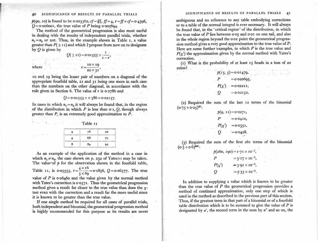
As an example of the application of the method in a case in which n1≠n2, the case shown on p. 232 of Yates(r) may be taken. The value of p for the observation shown in the fourfold table,
Table 11, is The true
value of P is 0.06460 and the value given by the normal method with Yates's correction is 0.0571. Thus the geometrical progression method gives a result far closer to the true value than does the X-test even with the correction and a result far the more useful since it is known to be greater than the true value.
If one single method be required for all cases of parallel trials, both independent and binomial, the geometrical progression method is highly recommended for this purpose as its results are never
In addition to supplying a value which is known to be greater than the true value of P the geometrical progression provides a method of continued approximation, only one step of which is used in the method as described in the previous part of this section. Thus, if the greatest term in that part of a binomial or of a fourfold table distribution which is to be summed to give the value of P is designated by a', the second term in the sum by a" and so on, the
(3) Required the sum of the first 261 terms of the binomial
(2) Required the sum of the last 12 terms of the binomial (0.75 + 0.25)20:
SIGNIFICANCE OF RESULTS OF PARALLEL TRIALS 41
ambiguous and no reference to any table embodying corrections or to a table of the normal integral is ever necessary. It will always be found that, in the 'critical region' of the distribution, in which the true value of P lies between 0.05 and 0.01 on one tail, and also in the whole region beyond the 0.01 point the geometrical progres-sion method gives a very good approximation to the true value of P . Here are some further examples, in which P is the true value and P(x') the approximation given by the normal method with Yates's correction.
(1) What is the probability of at least 15 heads in a toss of 20 coins?
40 SIGNIFICANCE OF RESULTS OF PARALLEL TRIALS
p(90, 10) is found to be 0.003362, Q = 0.006001, the true value of P being 0.005694.
The method of the geometrical progression is also most useful in dealing with the results of independent parallel trials, whether n1=n2 or not. Thus, in the example shown in Table 1, a value greater than P( ± 11) and which I propose from now on to designate by Q is given by
10 and 19 being the lesser pair of numbers on a diagonal of the appropriate fourfold table, 21 and 31 being one more in each case than the numbers on the other diagonal, in accordance with the rule given in Section 6. The value of r is 0.2786 and
In cases in which n1 = n2 it will always be found that, in the region of the distribution in which P is less than 0.1, Q, though always greater than P, is an extremely good approximation to P.
Table 11
42 SIGNIFICANCE OF RESULTS OF PARALLEL TRIALS
first multiplier or the ratio of a" to a' by r', the second multiplier by r" and so on, we have
and so on. Thus, in our example 3 of this section, omitting the factor 10-5 in the working,
Even with only two steps of approximation therefore a very good estimate of the true value of P has been obtained. It is, however, preferable to carry out at least three stages of approximation, to find out whether linear extrapolation is justifiable, if it is wished to estimate the value of P to a given degree of accuracy and not merely 'approximately'. Our estimates are 5.1624, 5.1697 and 5.1691, multiplied each by 10-5, according to the step in the approximation from which the estimate is made. It is safe, there-fore, to say that the true value of P is 5.17 to within ± 1 in the last figure.
SECTION 12. Suggestions as to choice of method of testing for significance in particular cases
(1) Fourfold table. n1 = n2 = n. n<30s
If n be less than 16 or is equal to 20 or 30, obtain exact value of P from Tables 2, 3 or 4. If n be not included in Tables 2, 3 or 4, for preliminary test use method of Section 3A. If working by a
Therefore our estimate of P is 5.1691 x 10⁻⁵. The true value of P, found by adding up the binomial terms, is
5.17 x 10⁻⁵ to two significant places of decimals, and the method of linear extrapolation gives the same result. Assuming now that we had carried out only the first two steps in the approximation we should have had, for the decrease in P ,
SIGNIFICANCE OF RESULTS OF PARALLEL TRIALS 43
In the above calculations d stands for the difference between the limits for the value of P. The method of linear extrapolation may be used to obtain the true value of P with a good degree of accuracy from the two last calculated values of the upper limit for P and the two last values of d. The difference between the values of d is 0.376 and that between the corresponding values of P is 0.028. Thus the corresponding decrease in P for a decrease in d from 1.060 to zero is

44 SIGNIFICANCE OF RESULTS OF PARALLEL TRIALS
fixed criterion and if the approximate value of P found by that method be well below the chosen critical value, it is not necessary to carry our further tests. If exact value of P be required or if working by decrease in value of P with additional trials, find exact values of P by methods of Sections 1 or 6.
(2) Fourfold table.
If s < 51 use method of Section 4A with Table 5. If s>50 use method of Section 11 to obtain Q, a value slightly greater than the true value of P.
(3) Fourfold table.
For preliminary trial use method of Section 11 to obtain Q. If significance doubtful and both n1 and n2 are less than 51, obtain exact value of P by method of Section 2 with Table 5, but, if either n1 or n2 are greater than 50, find value of P by method of Section 6. If both n1 and n2 are very large compared with s the method of Section 4B is applicable, but it is not possible to say how large the ratio n : s must be for this. The method of Section 11 will nearly always settle the question of significance. I f it does not it is necessary to find the exact value of P by the method of Section 6.
(4) Binomial cases. The symmetrical binomial, (0.5+0.5)n
For preliminary trial use the approximate method of Section 10. If significance is doubtful and if n be less than 51 use the exact method of Section 10 with Table 5. For values of n greater than 50 the normal method gives a value very near to the true value of P except when P is small ( < 0.05 for both tails together). In that case the method of Section 11 gives a better approximation and should be used when the approximate value given by the normal method is less than 0.06.
(5) Binomial cases. The asymmetrical binomial
For preliminary trial use the method of Section 11. If signi-ficance is doubtful the exact method of Section 10 must be used but it may be very laborious. The normal method is not applicable to asymmetrical binomials and may give very misleading results.
SIGNIFICANCE OF RESULTS OF PARALLEL TRIALS 45
SECTION 13. On the philosophical basis of tests for significance
It is a help, in understanding the basic theory of statistical tests, to form an imaginary model 'population' from which an observed value—a difference for instance—may be considered to be a ran-dom draw. A suitable model would be a heap of coloured balls, each difference being represented by balls of a particular colour, the number of balls of any colour being proportional to the pro-bability of the represented difference in the random sampling distribution. We shall assume that there are 10,000 balls altogether in the heap. Thus, for a difference, ±d, represented by red balls and having the probability, p, equal to 0.05, there will be 500 balls in the heap. There is a very large number of these heaps of balls, the number of colours and also the total number of balls in each being the same, but the proportional numbers of balls of each colour varying from one heap to another. In many of the heaps the proportional numbers of balls of each colour may, however, be the same. In one and only one kind of heap, type A, the number of balls of each colour is known but it is not known what proportion the number of heaps of this particular kind bears to the total number of heaps. In other words, it is quite impossible to estimate the probability that any particular heap is of the kind in question. The balls in each heap are assumed to have been thoroughly mixed together. We now draw a ball from one of the heaps, find that it is a red ball, and wish to decide whether it is reasonable to assume that it came from a heap of type A. We know, perhaps, that in a heap of this type there are 500 red balls and that there are alto-gether 200 balls of colours representing differences further from the 'expected' difference than that represented by red balls. In the type of distribution we are concerned with greater distance from the expected difference means lesser probability, so we can say that 200 is the total of balls represented less frequently than are red balls. We now have to decide whether the probability of drawing, from a heap of type A, a red ball or one of those less well represented is so small that it is very unlikely that the heap drawn from was of type A. We know perfectly well that, in many of the other heaps, there may be a far greater proportion of these balls than in the heaps of type A, and that our ball may be therefore much more likely to have been drawn from one of these others. We are only concerned, however, in deciding whether it can be considered as proved that it did not come from type A. By convention this

46 SIGNIFICANCE OF RESULTS OF PARALLEL TRIALS
proof is considered sufficiently strong if the number of balls in question is less than 5 % of the total number of balls. If the differences, + d and — d, have differing probabilities the observed positive difference and greater positive differences will be repre-sented by colours unlike those corresponding to the negative differences, and in that case the 'critical' proportion of balls is 2 .5%. It is open to any worker using statistical tests to employ values of P other than these as criteria of proof. It savours rather of arrogance to lay it down as a law that P < 0.05 shows 'significance' and that P<0.01 shows 'high significance', as if these concepts appeared suddenly with a given value of P. It is far better in published work, wherever possible, to give the true value of P and to leave it to the reader to decide whether the reality of an effect is proved to his satisfaction or not.
If the critical value, P=0.05 , be adhered to as deciding signi-ficance the decision that the reality of an effect is proved will be wrong on the average in one case in twenty trials, if the null hypothesis he really true. Since, however, there is no possible way of proving its truth one must not be misled into thinking that it will be true once in 20 times if, in each of twenty trials, the observed difference corresponds to the value 0.05 for P.
It should be noticed that the degree of conformity, shown by an observation, with the distribution defined by the null hypothesis is spoken of as showing the degree of likelihood of the truth of that hypothesis. The words 'probable' and 'probability' should never be used as if they were synonymous with 'likely' and 'likelihood'. Probability has an exact meaning in statistical theory, implicit in that meaning being the fact that all possibilities are known and that their relative chances of occurrence are calculable, at least approximately. Likelihood is merely a term measuring agreement between an observation and a particular hypothetical cause thereof and is in no way a measure of the probability of that cause. The two concepts are fundamentally different, likelihood having nothing whatever to do with chance of occurrence. One can compare likelihoods, say that one hypothetical cause of a result is more likely than another, and say that a certain hypothetical cause is the most likely of all hypothetical causes of the same type or, in other words, has maximum likelihood. Such values of likelihood are, how-ever, merely relatively comparable measures of conformity between certain chosen hypotheses and observed values and have nothing to do with the probability of the truth of those hypotheses, which are picked out from a completely unknown distribution of hypotheses.
SIGNIFICANCE OF RESULTS OF PARALLEL TRIALS 47
SECTION 14. Theoretical notes
(1) The origin of the binomial distribution
The binomial is the most important of the discontinuous dis-tributions. Its development is easy to follow and its logical basis simple. To understand the theory of the binomial is to be convinced that statistical methods are really founded on common-sense principles. The simplest case to which the binomial applies is that of a toss of a number of coins, and it will be assumed that five coins are to be used for illustrating our argument. It is necessary at first to distinguish the coins from each other, and we shall assume that they are marked with the letters A, B, C, D and E respec-tively. Now for any coin, for instance, A, the chances of a head or a tail are clearly equal to one another if there is absolutely no bias and the toss is carried out absolutely fairly. The probability of a head on any coin is therefore equal to ½, the chance of a head or a tail on any coin being equal to unity or certainty. Considering now a toss of two coins, A and B, there are four possible results, A(h) B(h), A(h) B(t), A(t) B(h), A(t) B(t), and the probability of a combination of any two particular independent events, for instance, A(h) and B(t), for each of which the probability is ½, is equal to ½ x ½. This is obvious from the fact that, if there are two ways of doing a thing once, there are four ways of doing it twice, eight ways of doing it three times and so on. It is an illustration of a funda-mental axiom in the theory of chance, namely, that the pro-bability of the simultaneous occurrence of n events, for each of which the probability is p, is equal to pn, or, in general, is equal to the product of the separate probabilities. Now let us consider alternative events. In the toss of two coins the event, one head and one tail, when the coins are not distinguished from one another, can occur in two ways, A(k) B(t) and A(t) B(h). This is an illustration of the axiom that the probability of one or other of two independent events is equal to the sum of the separate probabilities.
In the binomial distribution as applied to coins these are not distinguished from each other and the terms are usually arranged according to the number of 'successes'—heads, for instance—for which the corresponding term gives the probability. Thus the different results in a toss of two coins may be arranged in a binomial distribution as follows:
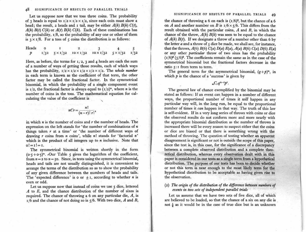
48 SIGNIFICANCE OF RESULTS OF PARALLEL TRIALS
Let us suppose now that we toss three coins. The probability of 3 heads is equal to 1/2 x 1/2 x 1/2, since each coin must show a head; the result, 2 heads and 1 tail, may be either A(h) B(h) C(t), A(h) B(t) C(h) or A(t) B(h) C(h). Each of these combinations has the probability, 1/8, so the probability of any one or other of them is 3 x 1/8. For a toss of 5 coins the distribution is as follows:
Here, as before, the terms for 1,2,3 and 4 heads are each the sum of a number of ways of getting those results, each of which ways has the probability, 1/2 x 1/2 x 1/2 x 1/2 x 1/2. The whole number in each term is known as the coefficient of that term, the other factor may be called the fractional factor. In the symmetrical binomial, in which the probability of a single component event is 1/2, the fractional factor is always equal to (1/2)n, where n is the number of coins in the toss. The mathematical equation for cal-culating the value of the coefficient is
in which n is the number of coins and r the number of heads. The expression on the left stands for ' the number of combinations of n things taken r at a time' or 'the number of different ways of drawing r coins from n coins', while n\ stands for 'factorial n' which is the product of all integers up to n inclusive. Note that O! = I ! = I .
The symmetrical binomial is written shortly in the form (0.5 +0.5)n . Our Table 5 gives the logarithm of the coefficient, from n = 2 to n = 50. Since, in tests using the symmetrical binomial, heads and tails are not usually distinguished, it is convenient to arrange the terms of the distribution so as to show the probability of any given difference between the numbers of heads and tails. The 'expected difference' is 0 or ±1, according to whether n is even or odd.
Let us suppose now that instead of coins we use 5 dice, lettered A to E, and the chance distribution of the number of sixes is required. The chance of throwing a 6 on any particular die, A, is 1/6 and the chance of not doing so is 5/6. With two dice, A and B,
The general law of chance exemplified by the binomial may be stated as follows: If an event can happen in a number of different ways, the proportional number of times it will happen in any particular way will, in the long run, be equal to the proportional number of times it can happen in that way. The truth of this law is self-evident. If in a very long series of throws with coins or dice the observed results do not conform more and more nearly with the appropriate binomial distribution as the number of throws is increased there will be every reason to suspect either that the coins or dice are biased or that there is something wrong with the method of throwing. The question of testing whether an apparent disagreement is significant or not is outside the scope of this paper, since the test is, in this case, for the significance of a discrepancy between a complete observed distribution and a complete theo-retical distribution, whereas every observation dealt with in this paper is considered in our tests as a single term from a hypothetical distribution. The purpose of our tests has been to decide whether or not this term is near enough to the most likely term for the hypothetical distribution to be acceptable as having given rise to the observation.
(2) The origin of the distribution of the difference between numbers of events in two sets of independent parallel trials
Let us assume that we have two sets of five dice, all of which are believed to be loaded, so that the chance of a six on any die is not 1/6 as it would be in the case of true dice but is an unknown
SIGNIFICANCE OF RESULTS OF PARALLEL TRIALS 49
the chance of throwing a 6 on each is (1/6)2, but the chance of a 6 on A and another number on B is 1/6 x 5/6. This differs from the result obtained with the particular coins, A and B, in which the chance of the throw, A(h) B{h) was seen to be equal to the chance of A(h) B(t). If we designate a throw of a number other than 6 by the letter a and a throw of 5 dice be made, we shall see, for instance, that the throws, A(6) B(6) C(a) D(a) E(a), A(a) B(6) C{a) D(6) E(a) or any other particular throw of two sixes has the probability (1/6)2 (5/6)3. The coefficients remain the same as in the case of the symmetrical binomial but the fractional factors decrease in the ratio 5:1 from term to term.
The general term for the asymmetrical binomial, (q+p)n, in which p is the chance of a 'success' is given by
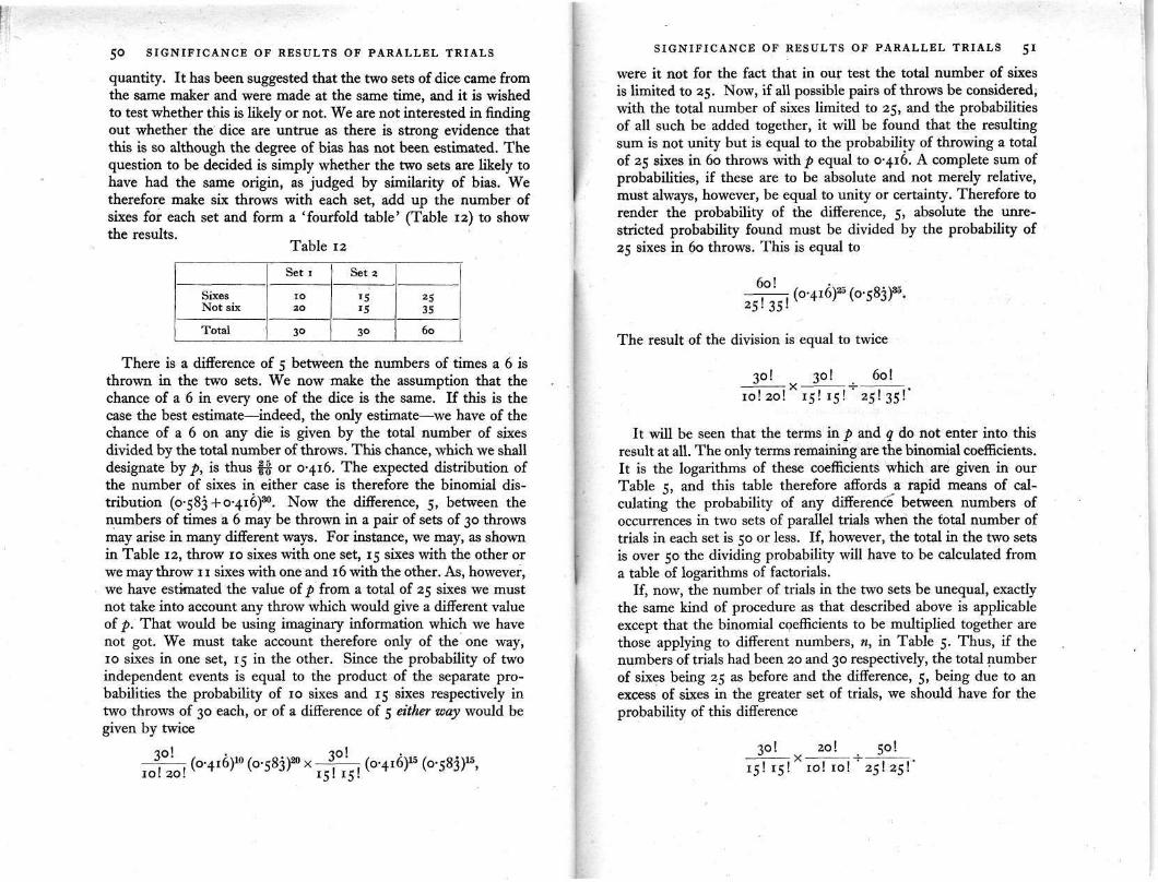
50 SIGNIFICANCE OF RESULTS OF PARALLEL TRIALS
quantity. It has been suggested that the two sets of dice came from the same maker and were made at the same time, and it is wished to test whether this is likely or not. We are not interested in finding out whether the dice are untrue as there is strong evidence that this is so although the degree of bias has not been estimated. The question to be decided is simply whether the two sets are likely to have had the same origin, as judged by similarity of bias. We therefore make six throws with each set, add up the number of sixes for each set and form a 'fourfold table' (Table 12) to show the results.
Table 12
There is a difference of 5 between the numbers of times a 6 is thrown in the two sets. We now make the assumption that the chance of a 6 in every one of the dice is the same. If this is the case the best estimate—indeed, the only estimate—we have of the chance of a 6 on any die is given by the total number of sixes divided by the total number of throws. This chance, which we shall designate by p, is thus 25/60 or 0.416. The expected distribution of the number of sixes in either case is therefore the binomial dis-tribution (0.583+ 0.416)30. Now the difference, 5, between the numbers of times a 6 may be thrown in a pair of sets of 30 throws may arise in many different ways. For instance, we may, as shown in Table 12, throw 10 sixes with one set, 15 sixes with the other or we may throw 11 sixes with one and 16 with the other. As, however, we have estimated the value of p from a total of 25 sixes we must not take into account any throw which would give a different value of p. That would be using imaginary information which we have not got. We must take account therefore only of the one way, 10 sixes in one set, 15 in the other. Since the probability of two independent events is equal to the product of the separate pro-babilities the probability of 10 sixes and 15 sixes respectively in two throws of 30 each, or of a difference of 5 either way would be given by twice
It will be seen that the terms in p and q do not enter into this result at all. The only terms remaining are the binomial coefficients. It is the logarithms of these coefficients which are given in our Table 5, and this table therefore affords a rapid means of cal-culating the probability of any difference between numbers of occurrences in two sets of parallel trials when the total number of trials in each set is 50 or less. If, however, the total in the two sets is over 50 the dividing probability will have to be calculated from a table of logarithms of factorials.
If, now, the number of trials in the two sets be unequal, exactly the same kind of procedure as that described above is applicable except that the binomial coefficients to be multiplied together are those applying to different numbers, n, in Table 5. Thus, if the numbers of trials had been 20 and 30 respectively, the total number of sixes being 25 as before and the difference, 5, being due to an excess of sixes in the greater set of trials, we should have for the probability of this difference
The result of the division is equal to twice
SIGNIFICANCE OF RESULTS OF PARALLEL TRIALS 51
were it not for the fact that in our test the total number of sixes is limited to 25. Now, if all possible pairs of throws be considered, with the total number of sixes limited to 25, and the probabilities of all such be added together, it will be found that the resulting sum is not unity but is equal to the probability of throwing a total of 25 sixes in 60 throws with p equal to 0.416. A complete sum of probabilities, if these are to be absolute and not merely relative, must always, however, be equal to unity or certainty. Therefore to render the probability of the difference, 5, absolute the unre-stricted probability found must be divided by the probability of 25 sixes in 60 throws. This is equal to
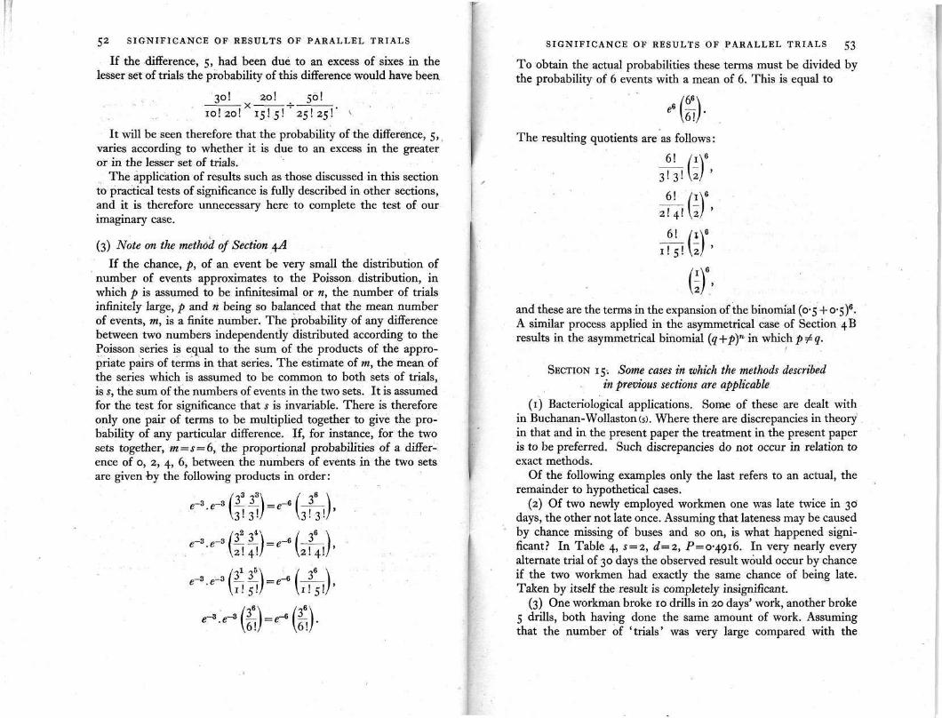
52 SIGNIFICANCE OF RESULTS OF PARALLEL TRIALS
If the difference, 5, had been due to an excess of sixes in the lesser set of trials the probability of this difference would have been
It will be seen therefore that the probability of the difference, 5, varies according to whether it is due to an excess in the greater or in the lesser set of trials.
The application of results such as those discussed in this section to practical tests of significance is fully described in other sections, and it is therefore unnecessary here to complete the test of our imaginary case.
(3) Note on the method of Section 4A If the chance, p, of an event be very small the distribution of
number of events approximates to the Poisson distribution, in which p is assumed to be infinitesimal or n, the number of trials infinitely large, p and n being so balanced that the mean number of events, m, is a finite number. The probability of any difference between two numbers independently distributed according to the Poisson series is equal to the sum of the products of the appro-priate pairs of terms in that series. The estimate of m, the mean of the series which is assumed to be common to both sets of trials, is s, the sum of the numbers of events in the two sets. It is assumed for the test for significance that s is invariable. There is therefore only one pair of terms to be multiplied together to give the pro-bability of any particular difference. If, for instance, for the two sets together, m=s=6, the proportional probabilities of a differ-ence of 0, 2, 4, 6, between the numbers of events in the two sets are given by the following products in order:
and these are the terms in the expansion of the binomial (0.5 + 0.5)6. A similar process applied in the asymmetrical case of Section 4B results in the asymmetrical binomial (q +p)n in which p ≠ q.
. .
SECTION 15. Some cases in which the methods described in previous sections are applicable
(1) Bacteriological applications. Some of these are dealt with in Buchanan-Wollaston (5). Where there are discrepancies in theory in that and in the present paper the treatment in the present paper is to be preferred. Such discrepancies do not occur in relation to exact methods.
Of the following examples only the last refers to an actual, the remainder to hypothetical cases.
(2) Of two newly employed workmen one was late twice in 30 days, the other not late once. Assuming that lateness may be caused by chance missing of buses and so on, is what happened signi-ficant? In Table 4, s = 2, d=2, P=0.4916. In very nearly every alternate trial of 30 days the observed result would occur by chance if the two workmen had exactly the same chance of being late. Taken by itself the result is completely insignificant.
(3) One workman broke 10 drills in 20 days' work, another broke 5 drills, both having done the same amount of work. Assuming that the number of 'trials' was very large compared with the
The resulting quotients are as follows:
SIGNIFICANCE OF RESULTS OF PARALLEL TRIALS 53
To obtain the actual probabilities these terms must be divided by the probability of 6 events with a mean of 6. This is equal to
S I G N I F I C A N C E OF RESULTS OF PARALLEL TRIALS 55
long caught by A, 23 were over 31 cm. long. Of those more than 25 cm. long caught by B, there were also 23 over 31 cm. long. Is there a significant difference between the ratios, number of soles 25.31 cm. long : number of soles over 31 cm. long in the two cases? The value of Q calculated by the method of Section 11 was found to be 0.007866, and therefore the difference is found to be highly significant.
LIST OF LITERATURE
(1) YATES, F. (1934). Contingency tables involving small numbers and the x2-test. (Supplement to J. Roy. Statist. Soc. vol. 1, no. 2.)
(2) PEARSON, KARL (1930). Tables for Statisticians and Biometricians. Part 1, Third edition. Cambridge University Press.
(3) FISHER, R. A. and YATES, F. (1938). Statistical Tables for Biological, Agricultural, and Medical Research. London: Oliver and Boyd.
(4) FISHER, R. A. (1934). Statistical Methods for Research Workers. Fifth or later edition. London: Oliver and Boyd.
(5) BUCHANAN-WOLLASTON, H. J. (1941). On tests for the significance of differences in degree of pollution by coliform bacteria and on the estimation of such differences. J. Hyg., Camb., vol. XLI, no. 2.
54 S I G N I F I C A N C E OF RESULTS OF PARALLEL TRIALS
number of breakages in each case and equal for both workmen, the method of Section 4A is applicable. P(±5) = 0.3018. The difference is quite insignificant.
(4) Of 15 drills broken in a particular test, 12 were of one make, 3 of another make, 30 of each being used altogether. In Table 4, s=15, d=9, P=0.007913. In less than one in a hundred trials would so great a difference arise by chance. It is assumed here that the trials were such as to give all drills the same chance of being broken.
(5) In a compound flower cyme there were found to be 40 sterile and 110 fertile florets. In a cyme of a related species there were 30 sterile and n o fertile florets. Is there a significant difference between the proportions of fertile to sterile florets? Find Q by method of Section 11 and, if necessary, carry out further steps in the approximation to P. It is assumed here that the chance of being fertile is the same for all florets in a cyme.
(6) In 10 randomly chosen cymes of one species there were 453 sterile and 1152 fertile florets. In 10 cymes of another species there were 312 sterile and 1264 fertile florets. Same test as in Ex. 5.
(7) Five water samples from various sites in Lake Windermere gave counts, respectively, of 10, 15, 30, 40 and 70 diatoms in a haemocytometer cell. Five samples taken from the same sites a week later gave counts, respectively, of 12, 20, 29, 45 and 85 diatoms in the cell. Was there a significant rise or fall in the diatom population of the sampled water masses? Test the counts of each set first of all by the x2 method to see whether it is reasonable to assume that they have arisen from the same Poisson distribution. If so, test for significance the difference between the total, 165, for the first set and the total, 191, for the second set. The methods of Section 10 of those of Section II may be used. If the numbers in either set are heterogeneous, find the values of P(d) and P(d+2) for the first two pairs of numbers by the exact method of Section 10 and, for the last three pairs, by the approximate method of that section. Calculate mean x for each pair and test total x for signi-ficance by method of Section 8. For the test for homogeneity and in the test of totals dilution must be the same for all samples. For the test of total x it is only necessary that dilution be the same for the two members of each pair.
(8) Two trawlers were fishing on the same grounds. Trawler A caught 56 soles over 25 cm. long in 7 hauls while trawler B caught 107 soles of over that length in 6 hauls. Of the soles above 25 cm.

CAMBRIDGE: PRINTED BY
WALTER LEWIS, M.A.
AT THE UNIVERSITY PRESS