Edda Leopold

On Semantic Spaces

1 Introduction

This contribution gives an overview about different approaches to semanticspaces. It is not a exhaustive survey, but rather a personal view on differentapproaches which use metric spaces for the representation of meanings oflinguistic units. The aim is to demonstrate the similarities of apparently differentapproaches and to inspire the generalisation of semantic spaces tailored to therepresentation of texts to arbitrary semiotic artefacts.

I assume that the primary purpose of a semiotic system is communication. Asemiotic system S consists of signs s. Signs fulfil a communicative function f (s)within the semiotic system in order to meet the communicative requirements ofsystem’s user. There are different similarity relations between functions of signs.In its most general form a semantic space can be defined as follows:

Definition 1.1 Let S be a semiotic system, (S, d) a metric space and r : S → S amapping from S to S. A semantic space (S, d) is a metric space whose elements arerepresentations of signs of a semiotic system, i.e. for each x ∈ S there is a s ∈ S suchthat r(s) = x. The inverse metric (d(x, y))−1 quantifies some functional similarity ofthe signs r−1(x) and r−1(y) in S.

Semantic spaces can quantify functional similarities in different respects. If thesemiotic system is a natural language, the represented units are usually wordsor texts — but semantic spaces can also be constructed from other linguisticunits like syllables or sentences. The constructions of Semantic spaces leads to anotion of semantic distance, which often cannot easily be made explicit. Someconstructions (like the one described in section 6) yield semantically transparentdimensions.

The definition of a semantic space is not confined to linguistic units. Anythingthat fulfils a function in a semiotic system can be represented in a semanticspace. The calculation of a semantic space often involves a reduction of dimen-sionality and the spaces described in this paper will be ordered with decreasingdimensionality and increasing semantic transparency. In the following sectionthe basic notations will be introduced, that are used in the subsequent sections.

LDV FORUM – Band 20 – 2005 63

Leopold

Section 3 roughly outlines the fuzzy linguistic paradigm. Sections 4 and 5describe shortly the methods of latent semantic indexing and probabilistic latentsemantic indexing. In section 6 I show how previously trained classifiers can beused in order to construct semantic spaces.

2 Notations

In order to harmonise the presentation of the different approaches I will use thefollowing notations: A text corpus C consists of a number of D different textualunits referred to as documents dj, j = 1, . . . , D. Documents can be complete texts,such as articles in a newspaper, short news as e.g. in the Reuters newswirecorpus, or even short text fragments like paragraphs or text blocks of a constantlength.

Each document consists of a (possibly huge) number of terms. The entirenumber of different term-types in C (i.e. the size of the vocabulary of C) isdenoted by W and the number of occurrences of a given term wi in a givendocument dj is denoted by f (wi, dj). The definition of what is considered asa term may vary, terms can be lemmas, words as they occur in the runningtext (i.e. strings separated by blanks), tagged words as for instance in Leopold& Kindermann (2002), strings of syllables as in Paaß et al. (2002), or evena mixture of lemmas and phrases as in Neumann & Schmeier (2002). Themethods described below are independent from what is considered as a termin a particular application. It is merely assumed that a corpus consists of aset of documents and each of these documents consist of a set of terms1. Theterm-document matrix A of C is a W × D matrix with W rows and D columns,which is defined as

A = ( f (wi, dj))i=1,...,W,j=,...,D

or more explicitly

A =

⎛⎜⎜⎜⎝

a11 a12 . . . a1Da21 a22 . . . a2D...

. . ....

aW1 aW2 . . . aWD

⎞⎟⎟⎟⎠ , where aij := f (wi, dj) (1)

1 Actually the assumption is even weaker: the methods simply focus on the co-occurrences ofdocuments and terms, no matter if one is contained in the other.

64 LDV-FORUM

On Semantic Spaces

The entry in the ith row and the jth column of the term-document matrixindicates how often term wi appears in document2 dj. The rows of A representterms and its columns represent documents. In the so-called bag-of-wordsrepresentation, document dj is represented by the jth column of A, which is alsocalled the word-frequency vector of document dj and denoted by �xj. The sumof the frequencies in the j-th row of A is denoted by f (dj), which is also calledthe length of document dj. The length of corpus C is denoted by L. Clearly

f (dj) =W

∑i=1

f (wi, dj) and L =D

∑j=1

f (dj) (2)

The ith row of A indicates how the term wi is spread over the documents inthe corpus. The rows of A are linked to the notion of polytexty, which wasdefined by Köhler (1986) as the number of contexts in which a given term wioccurs. Köhler noted that polytexty can be operationalised by the number oftexts the term occurs in i.e. the number of non-zero entries of the i-th row. Theith column of A is therefore called vector of polytexty of term wi and the vectorof the respective relative frequencies is named distribution of polytexty. The sumover the frequencies in the ith column, i.e. the total number of occurrences ofterm wi in the corpus C, is denoted by

f (wi) =D

∑j=1

f (wi, dj).

The polytexty measured in terms of non-zero entries in a row of the term-document matrix is also called document-frequency denoted as d f . The so-calledinverse document frequency, which was defined by Salton & McGill (1983) asid f = (log d f )−1, is widely used in the literature on automatic text processingin order to tune term-frequencies according to the thematic relevance of a term.Other term weighting schemes like e.g. the redundancy used by Leopold &Kindermann (2002) consider the entire vector of polytexty rather than solely thenumber of non-zero elements. An overview about different weighting schemesis given in Manning & Schütze (1999).

Matrix transposition, subsequently indicated by a superscript ·T , exchangescolumns and rows of a matrix. So the transposed term-document matrix is

2 It should be noticed here that in many cases the term-document matrix does not contain theterm-frequencies f (w, d) themselves but a transformation of them like e.g. log f (w, d) or tfdif.

Band 20 – 2005 65

Leopold

defined as

AT = ( f (wj, di))i=1,...,D,j=1,...,W =

⎛⎜⎜⎜⎝

at11 at

12 . . . at1W

at21 at

22 . . . at2W

.... . .

...at

D1 atW2 . . . at

DW

⎞⎟⎟⎟⎠ ,

where atij := f (wj, di)

It is easy to see that the matrix transposition is inverse to itself, i.e. (AT)T = A.All algorithms presented below are symmetric in documents and terms, i.e. theycan be used to estimate semantic similarity of terms as well as of documentsdepending on whether A or AT is considered.

There are various measures for judging the similarity of documents. Somemeasures — the so-called association measures — disregard the term frequenciesand just perform set-theoretical operations on the document’s term sets. Anexample for an association measure is the matching coefficient, which simplycounts the number of terms that two documents have in common (van Rijsbergen1975).

Other measures take advantage from the vector space model and considerthe entire term-frequency vectors of the respective documents. One of the mostoften used similarity measure, which is also mathematically convenient, is thecosine measure (Manning & Schütze 1999; Salton & McGill 1983) defined as

cos(�xi,�xj) =∑W

k f (wk, di) f (wk, dj)√∑W

k f (wk, di)2 ∑Wk f (wk, dj)2

=�xi ·�xj

‖�xi‖‖�xj‖ , (3)

which can also be interpreted as the angle between the vectors �xi and �xj or,up to centering, as the correlation between the respective discrete probabilitydistributions.

3 Fuzzy Linguistics

[. . .] the investigation of linguistic problems in general, and thatof word-semantics in particular, should start with more or less pre-theoretical working hypotheses, formulated and re-formulated forcontinuous estimation and/or testing against observable data, thenproceed to incorporate its findings tentatively in some preliminary

66 LDV-FORUM

On Semantic Spaces

theoretical set up which finally may perhaps get formalised to be-come part of an encompassing abstract theory. Our objective beingnatural language meaning, this operational approach would have tobe what I would like to call semiotic. (Rieger 1981)

Fuzzy Linguistics (Rieger & Thiopoulos 1989; Rieger 1981, 1999) aims at aspatial representation of word meanings. I.e. the units represented in thesemantic space are words as opposed to documents in the other approaches.However from a mathematical point of view there is no formal differencebetween semantic spaces that are constructed to represent documents and thosewhich are intended to represent terms. One can transform one problem into theother by simply transposing the term-document matrix i.e. by considering AT

instead of A.Rieger has calculated a semantic space of word meanings in two steps of

abstraction, which are also implicitly incorporated in the other constructions ofsemantic spaces described in the sections (4) to (6). The first step of abstraction isthe α-abstraction or more explicitly syntagmatic abstraction which reflects a term’susage regularities in terms of its vector of polytexty. The second abstractionstep is the δ-abstraction or paradigmatic abstraction, which represents a word’srelation to all other words in the corpus.

3.1 The Syntagmatic Abstraction

For each term wi a vector of length W is calculated, which contains the correla-tions of a term’s vector of polytexty with all other terms in the corpus.

αi,j =∑D

k=1( f (wi, dk) − E( f (wi) | dk))( f (wj, dk) − E( f (wj) | dk)√∑D

k=1( f (wi, dk) − E( f (wi) | dk))2 ∑Dk=1( f (wj, dk) − E( f (wj) | dk))2

(4)

where E( f (wi) | dk) = f (wi)f (dk)

L is an estimator of the conditioned expectationof the frequency of term wi in document dj, based on all documents in thecorpus. The coefficient αi,j measures the mutual affinity (αi,j > 0) or repugnancy(αi,j < 0) of pairs of terms in the corpus (Rieger & Thiopoulos 1989).

Substituting yi,j = f (wi, dk)− E( f (wi) | dk) the centralised vector of polytextyof term wi is defined as �yi = (yi,1, . . . , yi,D)T . Using this definition equation (4)can be rewritten as

Band 20 – 2005 67

Leopold

αi,j =∑D

k yi,kyj,k√∑D

k y2i,k ∑D

k y2j,k

=�yi ·�yj

‖�yi‖‖�yj‖ , (5)

which is the definition of the cosine distance as defined in equation (3). Thedifference between the α-abstraction and the cosine distance is merely that inequation (4) the centralised vector of polytexty is considered instead of theword-frequency vector in (3). Using the notion of polytexty one might say moreabstractly that αi,j is the correlation coefficient of the polytexty distributions ofthe types wi and wj on the texts in the corpus.

Syntagmatic abstraction realised by equation (4) refers to usage regularities interms of co-occurrences in the same document. Documents in Rieger’s workswere in general short texts, like e.g. newspaper texts (Rieger 1981; Rieger &Thiopoulos 1989) or small textual fragments (Rieger 2002). This means thatthe syntagmatic abstraction solely relies on the distribution of polytexty of therespective terms.

In principle however the approach can be generalised regarding varioustypes of generalised syntagmatic relations. Note that documents were definedas arbitrary disjoint subsets of a corpus. The underlying formal assumptionwas simply that there is a co-occurrence structure of documents and terms,which is represented in the term-document matrix. Consider for instance asyntactically tagged corpus. In such a corpus documents might be defined e.g.as a set of terms that all carry the same tag. The corresponding “distributions ofpolytexty” would describe how a term is used in different parts-of-speech andthe syntagmatic abstraction αi,j would measure the similarity of wi and wj interms of part-of-speech membership.

3.2 The Paradigmatic Abstraction

The α-abstraction measures the similarities of the distribution of polytexty overall terms in the corpus. The absolute value of the similarities, however, is notsolely a property of the terms themselves, but also of the corpus as a whole.That is if the corpus is confined to a small thematic domain, the documents willbe more similar than in the case of a corpus that covers a wide range of themes.In order to attain a paradigmatic abstraction, which abstracts away from thethematic coverage of the corpus, the Euclidean distances to all words in thecorpus are summed. This is the δ-abstraction (Rieger 1981; Rieger & Thiopoulos1989) given by:

68 LDV-FORUM

On Semantic Spaces

δ(yi, yj) =

√√√√ W

∑n=1

(αi,n − αj,n)2; δ ∈ [0; 2√

W] (6)

The δ-abstraction compensates the effect of the corpus’ coverage on α. Thesimilarity vector of each term is related to the similarity vectors of all otherterms in the corpus. In this way the paradigmatic structure in the corpus isevaluated in the sense that every term is paradigmatically related to each othersince every term can equally be engaged in a occurs-in-document relation.

So the vector yi, is mapped to a vector (δ(i, 1) . . . δ(i, W)), which containsthe Euclidean distance of xi’s α to all other αs generated by the corpus andis interpreted as meaning point in a semantic space (Rieger 1988). Riegerconcludes that in this way a semantic representation is attained that representsthe numerically specified generalised paradigmatic structure that has beenderived for each abstract syntagmatic usage regularity against all other in thecorpus (Rieger 1999).

Goebl (1991) uses another measurement to anchor similarity measurements oflinguistic units (in his case dialectometric data sets) for the completely differentpurpose of estimating the centrality of dialects in a dialectal network. Let αi,jdenote the similarity of dialect xi and xj, and let W denote the number ofdialects in the network. The centrality of xi is given by:

γ(xi) =W

∑n=1

(αi,n − 1

W

W

∑k=1

αi,k

)3(7)

He argues

The skewness of a similarity distribution has a particular linguis-tic meaning. The more symmetric a similarity distribution is, thegreater the centrality of the particular local dialect in the wholenetwork.(Goebl 1991)

Goebl uses (7) in order to calculate the centrality of a local dialect from the matrix(αi,j)i,j of similarity measures between pairs of dialects in the network. Thesecentrality measures are employed to draw a choropleth map of the dialectalnetwork. Substituting the delta abstraction in (6) by the skewness in (7) wouldresult in a measure for the centrality of a term in a term-document network:the more typical a term’s usage in the corpus the larger the value of γ. Such ameasure could be used as a term-weighting scheme.

Band 20 – 2005 69

Leopold

Rieger’s construction of a semantic space does not lead to a reduction of di-mensionality. This was not his aim. The meaning of a term is represented bya high-dimensional vector and thus demonstrates the complexity of meaningstructures in natural language. Rieger’s idea to compute semantic relations froma term-document matrix and represent semantic similarities as distances in ametric space has aspects in common with pragmatically oriented approacheslike e.g. latent semantic analysis. The measures of the αi,j can be written in amore condensed way as

B∗ = A∗(A∗)T = (αi,j)i,j=1,...W (8)

B∗ is a W × W-matrix which represents the similarity of the words wi and wj interms of their distribution of polytexty. The semantic similarity between wordsis calculated here in a way similar to the semantic similarity between words inlatent semantic indexing, which is described in the next section. The similaritymatrix B∗ = A∗(A∗)T however is calculated in a slightly different way. Theentries of A∗ are yi,j = f (wi, dk)− E( f (wi) | dk) rather than the term frequenciesf (wi, dj) themselves, as can be seen from equation (4).

More advanced techniques within the fuzzy linguistic paradigm (Mehler2002) extend the concept of the semantic space to the representation of texts.The respective computations, however, are complicated and exceed the scope ofthis paper.

Fuzzy linguistics aims at a numerical representation of the meaning of terms.Thus the paradigmatic abstraction in equation (6) does not involve a reduction ofdimensionality, in contrast to the principal component analysis that is performedin the paradigmatic abstraction step in latent semantic analysis. There is howevera close formal relationship.

4 Latent Semantic Analysis

In essence, and in detail, it [latent semantic analysis] assumes thatthe psychological similarity between any two words is reflected inthe way they co-occur in small subsamples of language. (Landauer& Dumais (1997); Words in square brackets added by the author.)

In contrast to fuzzy linguistics latent semantic analysis (LSA) is interested in thesemantic nearness of documents rather than of words. The method however issymmetric and can be applied to the similarity of words as well.

70 LDV-FORUM

On Semantic Spaces

LSA projects Document frequency vectors into a low dimensional space calcu-lated using the frequencies of word occurrence in each document. The relativedistances between these points are interpreted as distances between the topicsof the documents and can be used to find related documents, or documentsmatching some specified query (Berry et al. 1995). The underlying technique ofLSA was chosen to fulfil the following criteria:

1. To represent the underlying semantic structure a model with sufficientpower is needed. Since the right kind of alternative is unknown the powerof the model should be variable.

2. Terms and documents should both be explicitly represented in the model.

3. The method should be computationally tractable for large data sets. Deer-wester et al. concluded that the only model which satisfied all thesethree criteria was the singular value decomposition (SVD), which is a wellknown technique in linear algebra (Deerwester et al. 1990).

4.1 Singular Value Decomposition

Let A be a term-document matrix as defined in section (2) with rank3 r. Thesingular value decomposition of A is given by

A = UΣV, (9)

where Σ = diag(σ1, . . . , σr) is a diagonal matrix with ordered diagonal elementsσ1 > . . . > σr,

U =

⎛⎜⎜⎜⎝

u11 u12 . . . u1ru21 u22 . . . u2r

.... . .

...uW1 uW2 . . . uWr

⎞⎟⎟⎟⎠

is a W × r-matrix with orthonormal columns and

V =

⎛⎜⎜⎜⎝

v11 v12 . . . v1rv21 v22 . . . v2r

.... . .

...vr1 vr2 . . . vrr

⎞⎟⎟⎟⎠

3 In practice one can assume r = D, since it is very unlikely that there are two documents in thecorpus with linear dependent term-frequency vectors

Band 20 – 2005 71

Leopold

is a r × r-matrix with orthonormal rows. The diagonal elements σ1, . . . , σr ofthe matrix Σ are singular values of A. The singular value decomposition canequivalently be written as an eigen-value decomposition of the similarity matrix

B = AAT (10)

Note that U and V are orthonormal matrices therefore UUT = I and VVT = I,where I is the neutral element of matrix-multiplication. According to (9) thesingular value decomposition of the transposed term-document matrix AT isobtained as AT = VTΣUT . Hence AAT = UΣVVTΣUT = UΣ2UT which is theeigen-value decomposition of AAT with eigen-values σ2

1 , . . . , σ2r . Term frequency

vectors are mapped to the latent space of artificial concepts by multiplicationwith UΣ, i.e. �x → �xTUΣ. Each of the r dimensions of the latent space maybe thought of as an artificial concept, which represents common meaningcomponents of different words and documents.

4.2 Deleting the Smallest Singular Values

A reduction of dimensionality is achieved by deleting the smallest singularvalues corresponding to the less important concepts in the corpus. In so doinglatent semantic analysis reduces the matrix A to a smaller K-dimensional (K < r)matrix

AK = UKΣKVK, (11)

where UK and VK are obtained from U and V in equation (9) by deletingrespectively columns and/or rows K + 1 to r and the diagonal matrix is reducedto ΣK = diag(σ1, . . . , σK). The mapping of a term-frequency vector to thereduced latent space is now performed by �x → �xTUKΣK. It has been found thatK ≈ 100 is a good value to chose for K (Landauer & Dumais 1997).

LSA leads to vectors with few zero entries and to a reduction of dimensionality(k instead of W) which results in a better geometric interpretability. This impliesthat it is possible to compute meaningful association values between pairs ofdocuments, even if the documents do not have any terms in common.

4.3 SVD Minimises Euclidean Distance

Truncating the singular value decomposition as described in equation (11)projects the data onto the best-fitting affine subspace of a specified dimension K.It is a well-known theoretical result in linear algebra, that there is no matrix X

72 LDV-FORUM

On Semantic Spaces

with rank(X) < K that has a smaller Frobenius distance to the original matrixA i.e. AK minimises

‖A − AK‖F =K

∑i,j

(ai,j − aKi,j)

2. (12)

Interestingly Rieger’s δ-abstraction in equation (6) yields a nice interpretationof this optimality statement. The reduction of dimensionality performed bylatent semantic analysis is achieved in such a way that it optimally preserves theinherent meaning (i.e. the sum of the δ(xi, xj)). That is the meaning points in theRieger’s δ-space are changed to the minimal possible extent. Another parallelbetween fuzzy linguistics and LSA is that equation (4) and the correspondingmatrix notation of αi,j in equation (8) coincide withe the similarity matrix inequation (10). The only difference is that the entries of A and A∗ are definedin a different way. Using Rieger’s terminology one may call equation (10) asyntagmatic abstraction, because it reflects the usage regularities in the corpus.The singular value decomposition is then the paradigmatic abstraction, since itabstracts away from the paradigmatic structure of the language’s vocabularywhich consists of synonymy and polysemy relationships.

One objection to latent semantic indexing is that, along with all other least-square methods, the property of minimising the Frobenius distance makesit suited for normally distributed data. The normal distribution however isunsuitable to model term frequency counts. Other distributions like Poisson ornegative binomial are more appropriate for this purpose (Manning & Schütze1999).

Alternative methods have therefore been developed (Gous 1998), whichassume that the term frequency vectors are multinomially distributed andtherefore agree with well corroborated models on word frequency distributiondeveloped by Chitashvili and Baayen (Chitashvili & Baayen 1993). ProbabilisticLatent Semantic Analysis has advanced further in this direction.

5 Probabilistic Latent Semantic Analysis

Whereas latent semantic analysis is based on counts of co-occurrences and usesthe singular value decomposition to calculate the mapping of term-frequencyvectors to a low-dimensional space, probabilistic latent semantic analysis (seeHofmann & Puzicha (1998); Hofmann (2001)) is based on a probabilistic frame-work and uses the maximum likelyhood principle. This results in a better lin-

Band 20 – 2005 73

Leopold

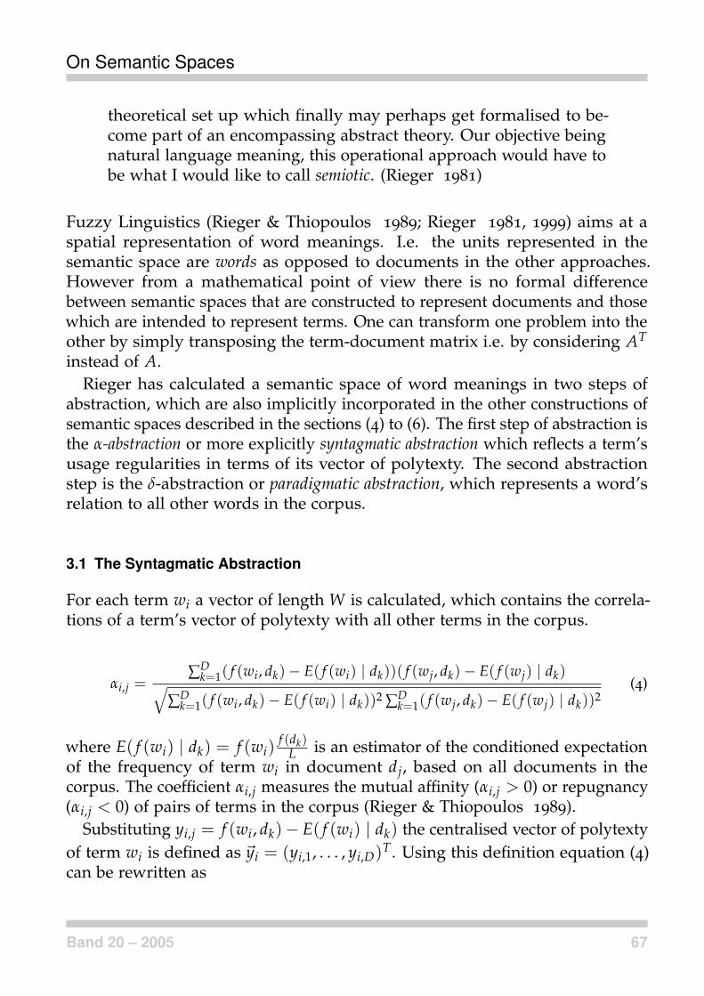
guistic interpretability and makes probabilistic latent semantic analysis (PLSA)compatible with the well-corroborated multinomial model of word frequencydistributions.

5.1 The Multinomial Model

The assumption that the occurrences of different terms in the corpus are stochas-tically independent allows to calculate the probability of a given term frequencyvector �xj = ( f (w1, dj), . . . , f (wW , dj)) according to the multinomial distribution(see Chitashvili & Baayen (1993); Baayen (2001)):

p(�xj) =f (dj)

∏Wi=1 f (wi, dj)!

W

∏i=1

p(wi, dj)f (wi ,dj)

If it is further assumed that the term-frequency vectors of the documents inthe corpus are stochastically independent, the probability to observe a giventerm-document matrix is

p(A) =D

∏j=1

f (dj)W∏i=1

f (wi, dj)!

W

∏i=1

p(wi, dj)f (wi ,dj) (13)

5.2 The Aspect Model

In order to map high-dimensional term-frequency vectors to a limited num-ber of dimensions PLSA uses a probabilistic framework, called aspect model.The aspect model is a latent variable model which associates an unobservedclass variable zk, k = 1, . . . , K, with each observation an observation being theoccurrence of a word in a particular document. The latent variables zk can bethought of as artificial concepts like the latent dimensions in LSA. Like in LSAthe number of artificial concepts K has to be chosen by the experimenter. Thefollowing probabilities are introduced: p(dj) denotes the probability that a wordoccurrence will be observed in a particular document di, p(wi | zk) denotesthe conditional probability of a specific term conditioned on the latent variablezk (i.e. the probability of term wi given the thematic domain zk), and finallyp(zk | dj) denotes a document-specific distribution over the latent variable spacei.e. the distribution of artificial concepts in document dj. A generative modelfor word/document co-occurrences is defined as follows:

74 LDV-FORUM

On Semantic Spaces

(1) select a document dj with probability p(dj),

(2) pick a latent class zk with probability p(zk|dj), and

(3) generate word wj with probability p(wi|zk) (Hofmann 2001).

Since the aspects are latent variables which cannot be observed directly, theconditioned probability p(wi | dj) has to be calculated as the sum of the possibleaspects:

p(wi|dj) =K

∑k=1

p(wi|zk)p(zk|dj) (14)

This implies the assumption, that the conditioned probability of occurrence ofaspect zk in document dj is independent from the conditioned probability thatterm wi is used given that aspect zk is present (Hofmann 2001).

In order to find the optimal probabilities p(wi|zk) and p(zk|dj), maximizingthe probability of observing a given term-document matrix, the maximumlikelihood principle is applied. The multinomial coefficient in equation (13)remains constant when the probabilities p(wi, dj) are varied. It can therefore beomitted for the calculation of the likelihood function, which is then given as

L =D

∑j=1

W

∑i=1

f (wi, dj) log p(wi, dj)

Using the definition of the conditioned probabilities p(wi, dj) = p(dj)p(wi | dj)and inserting equation (14) yields

L =D

∑j=1

W

∑i=1

(f (wi, dj) log

(p(dj) ·

K

∑k=1

p(wi | zk)p(zk | dj)))

Using the additivity of the logarithm and factoring in f (wi, dj) gives

L =D

∑j=1

(W

∑i=1

f (wi, dj) log p(dj) +W

∑i=1

f (wi, dj) logK

∑k=1

p(wi | zk)p(zk | dj)

)

Band 20 – 2005 75

Leopold

Since ∑i f (wi, dj) = f (dj) factoring out f (dj) finally leads to the likelihoodfunction

L =D

∑j=1

f (dj)

(log p(dj) +

W

∑i=1

f (wi, dj)f (dj)

logK

∑k=1

p(wi | zk)p(zk | dj)

)(15)

which has to be maximised with respect to the conditional probabilities involvingthe latent aspects zk. Maximisation of (15) can be achieved using the EM-algorithm, which is a standard procedure for maximum likelihood estimationin latent variable models (Dempster et al. 1977). The EM-algorithm works intwo steps that are iteratively repeated (see e.g. Mitchell (1997) for details).

Step 1 In the first step (the expectation step) the expected value E(zk) of thelatent variables is calculated, assuming that the current hypothesis h1holds.

Step 2 In a second step (the maximisation step) a new maximum likelihoodhypothesis h2 is calculated assuming that the latent variables zk equal theirexpected values E(zk) that have been calculated in the expectation step.Then h1 is substituted by h2 and the algorithm is iterated.

In the case of PLSA the the EM-algorithm is employed as follows (see Hofmann(2001) for details): To initialise the algorithm generate W · K random valuesfor the probabilities p(wi | zk) and D · K random values for the probabilitiesp(zk | dj) such that all probabilities are larger than zero and fulfil the conditions∑i,k p(wi | zk) = 1 and ∑j,k p(zk | dj) = 1 respectively. The expectation step canbe obtained from equation (15) by applying Bayes’ formula:

p(zk | wi, dj) =p(wi | zk)p(zk | dj)

∑Kk=1 p(wi | zk)p(zk | dj)

(16)

In the maximization step the probability p(zk | wi, dj) is used to calculate thenew conditioned probabilities

p(wi | zk) =∑N

j=1 f (wi, dj)p(zk | wi, dj)

∑Kk=1 ∑D

j=1 f (wi, dj)(zk | wi, dj)(17)

and

76 LDV-FORUM

On Semantic Spaces

p(zk | dj) =∑W

i=1 f (wi, dj)p(zk | wi, dj)f (dj)

, (18)

Then the conditioned probabilities p(zk|dj) and p(wi|zk) calculated from equa-tion (17) and (18) are inserted into equation (16) to perform the next iteration.The iteration is stopped when a stationary point of the likelihood function isachieved. The probabilities p(zk | dj), k = 1, . . . , K, uniquely define for eachdocument a K − 1-dimensional point in continuous latent space.

It is reported that PLSA outperforms LSA in terms of perplexity reduction.Notably PLSA allows to train latent spaces with a continuous increase in per-formance, in contrast to LSA where the model perplexity increases when acertain number of latent dimensions is exceeded. In PLSA the number of latentdimensions may even exceed the rank of the term-document matrix (Hofmann2001).

The main difference between LSA and PLSA is the optimisation criterionfor the mapping to the latent space, which is defined by UΣ and p(zk | dj)respectively. LSA minimises the least square criterion in equation (12) andthus implicitly assumes an additive Gaussian noise on the term-frequency data.PLSA in contrast assumes multinomially distributed term-frequency vectorsand maximises the likelihood of the aspect model. It is therefore in accordancewith linguistic word frequency models. One disadvantage of PLSA is, that theEM-algorithm like most iterative algorithms converges only locally. Thereforethe solution need not be a global optimum, in contrast to LSA which uses analgebraic solution and ensures global optimality.

6 Classifier Induced Semantic Spaces

[. . .] problems, in which the task is to classify examples into one of adiscrete set of possible categories, are often referred to as classificationproblems.(Mitchell 1997)

The main problem in PLSA approach was to find the latent aspect variables zkand calculate the corresponding conditioned probabilities p(wi|zk) and p(zk|dj).It was assumed that the latent variables correspond to some artificial concepts. Itwas impossible however to specify these concepts explicitly. In the approach de-scribed below, the aspect variables can be interpreted semantically. Prerequisitefor such a construction of a semantic space is a semantically annotated trainingcorpus. Such annotations are usually done manually according to explicitly

Band 20 – 2005 77

Leopold

defined annotation rules. An example of such a corpus is e.g. the news data ofthe German Press Agency (dpa) which is annotated according to the categoriesof the International Press Telecommunications Council (IPTC). These annota-tions inductively define the concepts zk, or the dimensions, of the semanticspace. A classifier induced semantic space (CISS) is generated in two steps: In thetraining step classification rules �xj → zk are inferred from the training data. Inthe classification step these decision rules are applied to possibly unannotateddocuments.

This construction of a semantic space is especially useful for practical appli-cations because (1) the space is low-dimensional (up to dozens of dimensions)and thus can easily be visualised, (2) the space’s dimension possesses a welldefined semantic interpretation, and (3) the space can be tailored to the specialrequirements of a specific application. The disadvantage of classifier inducedsemantic spaces (CISS) is that they rely on supervised classifiers. Thereforemanually annotated training data is required.

Classification algorithms often use an internal representation of degree ofmembership. They internally calculate how much a given input vector �x belongsto a given class zk. This internal representation of degree of membership can beexploited to generate a semantic space.

A Support Vector Machine (SVM) is a supervised classification algorithmthat recently has been applied successfully to text classification tasks. SVMshave proven to be an efficient and accurate text classification technique (Dumaiset al. 1998; Drucker et al. 1999; Joachims 1998; Leopold & Kindermann2002). Therefore Support Vector Machines appears to be the best choice for theconstruction of a semantic space for textual documents.

6.1 Using an SVM to Quantify the Degree of Membership

Like other supervised machine learning algorithms, an SVM works in two steps.In the first step — the training step — it learns a decision boundary in inputspace from preclassified training data. In the second step — the classificationstep — it classifies input vectors according to the previously learned decisionboundary. A single support vector machine can only separate two classes — apositive class (y = +1) and a negative class (y = −1). This means that for eachof the K classes zk a new SVM has to be trained separating zk from all otherclasses.

In the training step the following problem is solved: Given is a set of trainingexamples S� = {(�x1, y1), (�x2, y2), . . . , (�x�, y�)} of size � ≤ W from a fixed butunknown distribution p(�x, y) describing the learning task. The term-frequency

78 LDV-FORUM

On Semantic Spaces

class +1

class -1

margin

separating hyperplanew*x+b=0

w*x+b<-1

w*x+b>1 ξ

kv

Figure 1: Generating a CISS with a support vector machine. The SVM algorithmseeks to maximise the margin around a hyperplane that separate a positiveclass (marked by circles) from a negative class (marked by squares). Oncean SVM is trained, vk = �wk�x + b is calculated in the classification step. Thequantity vk measures the rectangular distance between the point marked by astar and the hyperplane. It can be used to generate a CISS.

vectors �xi represent documents and yi ∈ {−1, +1} indicates whether a documenthas been annotated as belonging to the positive class or not. The SVM aims tofind a decision rule hL : �x → {−1, +1} based on S� that classifies documents asaccurately as possible.

The hypothesis space is given by the functions f (�x) = sgn(�w�x + b), where �wand b are parameters that are learned in the training step and which determinethe class separating hyperplane. Computing this hyperplane is equivalent tosolving the following optimisation problem (Vapnik 1998; Joachims 2002):

minimise: V(�w, b,�ξ) =12�w�w + C

�

∑i=1

ξi

subject to: ∀�i=1 : yi(�w�x + b) ≥ 1 − ξi

∀�i=1 : ξi ≥ 0

Band 20 – 2005 79

Leopold

The constraints require that all training examples are classified correctly allowingfor some outliers, symbolised by the slack variables ξi. If a training examplelies on the wrong side of the hyperplane, the corresponding ξi is greater orequal to 0. The factor C is a parameter that allows one to trade off training erroragainst model complexity. Instead of solving the above optimization problemdirectly, it is easier to solve the following dual optimisation problem (Vapnik1998; Joachims 2002).

minimise: W(�α) = −�

∑i=1

αi +12

�

∑i=1

�

∑j=1

yiyjαiαj�xi�xj

subject to:�

∑i=1 0

≤ αi≤C

yiαi = 0 (19)

All training examples with αi > 0 at the solution are called support vectors. Thesupport vectors are situated right at the margin (see the solid squares and thecircle in figure (1)) and define the hyperplane. The definition of a hyperplaneby the support vectors is especially advantageous in high dimensional featurespaces because a comparatively small number of parameters — the αs in thesum of equation (19) — is required.

In the classification step an unlabeled term-frequency vector is estimated tobelong to the class

y = sgn(�w�x + b) (20)

Heuristically the estimated class membership y corresponds to whether �x be-longs on the lower or upper side of the decision hyperplane. Thus estimatingthe class membership by equation (20) consists of a loss of information sinceonly the algebraic sign of right-hand term is evaluated. However the value ofv = �w�x + b is a real number and can be used in order to create a real valuedsemantic space, rather than just to estimate if �x belongs to a given class or not.

6.2 Using Several Classes to Construct a Semantic Space

Suppose there are several, say K, classes of documents. Each document isrepresented by an input vector �xj. For each document the variable yk

j ∈ {−1, +1}indicates whether �xj belongs to the k-th class (k = 1, . . . , K) or not. For eachclass k = 1, . . . , K an SVM can be learned which yields the parameters �wk and

80 LDV-FORUM

On Semantic Spaces

bk. After the SVMs have been learned, the classification step (equation (20)) canbe applied to a (possibly unlabeled) document represented by �x resulting ina K-dimensional vector �v, whose kth component is given by vk = �wk · �x + bk

The component vk quantifies how much a document belongs to class k. Thusthe document represented by the term frequency vector �xj is mapped to theK-dimensional vector in the classifier induced semantic space. Each dimensionin this space can be interpreted as the membership degree of the document toeach of the K classes.

−2 −1 0 1 2 3

−2

−1

01

2

disaster

cultu

re

−2 −1 0 1 2 3

−2

−1

01

2

justice

cultu

re

Figure 2: A classifier induced semantic space. 17 classifiers have been trainedaccording to the highest level of the IPTC classification scheme. The projectionto two dimensions “culture” and “disaster” is displayed on the right, and theprojection to “culture” and “justice” on the left. The calculation is based on68778 documents from the “Basisdienst” of the German Press Agency (dpa)July-October 2000.

The relation between PLSA and CISS is given by the latent variable zk. In thecontext of CISS the latent variable zk is interpreted as the thematic domain, inaccordance with semantic annotations in the corpus. Statistical learning theoryassumes, that each class k is learnable because there is an underlying conditional

Band 20 – 2005 81

Leopold

distribution p(�xj | zk), which reflects the special characteristics of the class zk.The classification rules that are learned from the training data minimise theexpected error. In PLSA the aspect variables are not previously defined. Theconditioned probabilities p(wi | zk) and p(zk | �xj) are chosen in such a way thatthey maximise the likelihood of the multinomial model.

6.3 Graphical Representation of a CISS

Self-organising Maps (SOM) were invented in the early 80s (Kohonen 1980).They use a specific neural network architecture to perform a recursive regressionleading to a reduction of the dimension of the data. For practical applicationsSOMs can be considered as a distance preserving mapping from a more thanthree-dimensional space to two-dimensions. A description of the SOM algorithmand a thorough discussion of the topic is given by Kohonen (1995).

Figure 3 shows an example of a SOM visualising the semantic relations ofnews messages. SVMs for the four classes ’culture’, ’economy’, ’politics’, and’sports’ were trained by news messages from the ’Basisdienst’ of the GermanPress Agency (dpa) April 2000. Classification and generation of the SOM wasperformed for the news messages of the first 10 days of April. 50 messageswere selected at random and displayed as white crosses. The categories areindicated by different grey tone. Then the SOM algorithm is applied (with100 × 100 nodes using Euclidean metric) in order to map the four-dimensionaldocument representations to two dimensions admitting a minimum distortionof the distances. The grey tone indicates the topic category. Shadings within thecategories indicate the confidence of the estimated class membership (dark =low confidence, bright = high confidence).

It can be seen that the change from sports (15) to economy (04) is filled bydocuments which cannot be assigned confidently to either classes. The areabetween politics (11) and economy (04), however, contains documents, whichdefinitely belong to both classes. Note that classifier induced semantic spacesgo beyond a mere extrapolation of the annotations found in the training corpus.It gives an insight into how typical a certain document is for each of the classes.Furthermore Classifier induced semantic spaces allow one to reveal previouslyunseen relationships between classes. The bright islands in area 11 on Figure 3show, for example, that there are messages classified as economy which surelybelong to politics.

82 LDV-FORUM

On Semantic Spaces

Figure 3: Self-organising map of a classifier induced semantic space. 4 classi-fiers have been trained according to the highest level of the IPTC classificationscheme. The shadings and numbers indicate the “true” topic annotations ofthe news messages. 01: culture, 04: economy, 11: politics, 15: sports. (Thefigure was taken from Leopold et al. (2004)).

7 Conclusion

Fuzzy Linguistics, LSA, PLSA, and CISS map documents to the semantic spacein a different manner. Fuzzy Lintuistics computes a vector for each wordwhich consists of the cosine distances to every other word in the corpus. Thenit calculates the Euclidean Dinstances between the vectors which gives themeaning point. Documents are represented by summing up the meaning pointsof the document’s words.

Band 20 – 2005 83

Leopold

In the case of LSA the representation of the document in the semantic spaceis achieved by matrix multiplication: dj → �xT

j UKΣK. The dimensions of thesemantic space correspond to the K largest eigen-values of the similarity matrixAAT . The projection employed by LSA always leads to a global optimum interms of the Euclidean distance between A and Ak.

PLSA maps a document to the vector of the conditional probabilities, whichindicate how probable aspect zk is, when document dj is selected: dj → (p(z1 |dj), . . . , p(zK | dj)). The probabilities are derived from the aspect model usingthe maximum likelihood principle and the assumption of multinomially dis-tributed word frequency distributions. The the likelihood function is maximisedusing the EM-algorithm, which is an iterative algorithm that leads only to alocal optimum.

CISS requires a training corpus of documents annotated according to theirmembership of classes zk. The classes have to be explicitly defined by the humanannotation rules. For each class zk a classifier is trained, i.e. parameters �wk and bk

are calculated from the training data. For each document dj the quantities vk =�wk ·�x + bk are calculated, which indicate how much dj belongs the previouslylearned classes zk. The mapping of document dj to the semantic space isdefined as dj → (v1, . . . vK). The dimensions can be interpreted according to theannotation rules.

8 Acknowledgements

This study is part of the project InDiGo which is funded by the German ministry forresearch and technology (BMFT) grant number 01 AK 915 A.

References

Baayen, H. (2001). Word Frequency Distributions. Dordrecht: Kluwer.

Berry, M. W., Dumais, S. T., & O’Brien, G. W. (1995). Using linear algebra for intelligentinformation retrieval. SIAM Review, 37(4), 573–595.

Chitashvili, R. J. & Baayen, R. H. (1993). Word frequency distributions. In G. Altmann &L. Hrebícek (Eds.), Quantitative Text Analysis (pp. 54–135). Trier: wvt.

Deerwester, S., Dumais, S. T., Furnas, G. W., Landauer, T. K., & Harshmann, R. (1990).Indexing by latent semantic analysis. Journal of the American Society for InformationScience, 41(6), 391–407.

84 LDV-FORUM

On Semantic Spaces

Dempster, A. P., Laird, N. M., & Rubin, D. B. (1977). Maximum likelihood from in-complete data via the EM algorithm. Journal of the Royal Statistical Society, B, 39,1–38.

Drucker, H., Wu, D., & Vapnik, V. (1999). Support vector machines for spam categoriza-tion. IEEE Transactions on Neural Networks, 10, 1048–1054.

Dumais, S., Platt, J., Heckerman, D., & Sahami, M. (1998). Inductive learning algorithmsand representations for text categorization. In Proceedings of the ACM-CIKM, (pp.148–155).

Goebl, H. (1991). Dialectrometry: A short overview of the principles and practice ofquantitative classification of linguistic atlas data. In Köhler, R. & Rieger, B. B. (Eds.),Contributions to quantitative linguistics, Proceedings of the first international conferenceon quantitative linguistics, (pp. 277–315)., Dordrecht. Kluwer.

Gous, A. (1998). Exponential and Spherical Subfamily Models. PhD thesis, Stanford Univer-sity.

Hofmann, T. (2001). Unsupervised learning by probabilistic latent semantic analysis.Machine Learning, 42, 177–196.

Hofmann, T. & Puzicha, J. (1998). Statistical models for co-occurrence data. A.I. MemoNo. 1625., Massachusetts Institute of Technology.

Joachims, T. (1998). Text categorization with support vector machines: learning withmany relevant features. In Proceedings of the Tenth European Conference on MachineLearning (ECML 1998), (pp. 137–142)., Berlin. Springer.

Joachims, T. (2002). Learning to classify text using support vector machines. Boston: Kluwer.Köhler, R. (1986). Zur linguistischen Synergetik: Struktur und Dynamik der Lexik. Bochum:

Brockmeyer.Kohonen, T. (1980). Content-addressable Memories. Berlin: Springer.Kohonen, T. (1995). Self-Organizing Maps. Berlin: Springer.Landauer, T. K. & Dumais, S. T. (1997). A solution to plato’s problem: The latent

semantic analysis theory of acquisition, induction, and representation of knowledge.Psychological Review, 104(2), 211–240.

Leopold, E. & Kindermann, J. (2002). Text categorization with support vector machines.How to represent texts in input space? Machine Learning, 46, 423–444.

Leopold, E., May, M., & Paaß, G. (2004). Data mining and text mining for science andtechnology research. In H. F. Moed, W. Glänzel, & U. Schmoch (Eds.), Handbook ofQuantitative Science and Technology Research (pp. 187–214). Dordrecht: Kluwer.

Manning, C. D. & Schütze, H. (1999). Foundations of Statistical Natural Language Processing.Cambridge, Massachusetts: MIT Press.

Mehler, A. (2002). Hierarchical orderings of textual units. In Proceedings of the 19thInternational Conference on Computational Linguistics, COLING’02, Taipei, (pp. 646–652)., San Francisco. Morgan Kaufmann.

Band 20 – 2005 85

Mitchell, T. M. (1997). Machine Learning. New York: McGraw-Hill.

Neumann, G. & Schmeier, S. (2002). Shallow natural language technology and textmining. Künstliche Intelligenz, 2(2), 23–26.

Paaß, G., Leopold, E., Larson, M., Kindermann, J., & Eickeler, S. (2002). SVM classificationusing sequences of phonemes and syllables. In Proceedings of the 6th EuropeanConference on Principles of Data Mining and Knowledge Discovery (PKDD), Helsinki, (pp.373–384)., Berlin. Springer.

Rieger, B. B. (1981). Feasible fuzzy semantics. On some problems of how to handle wordmeaning empirically. In H. Eikmeyer & H. Rieser (Eds.), Words, Worlds, and Contexts.New Approaches in Word Semantics (Research in Text Theory 6) (pp. 193–209). Berlin: deGruyter.

Rieger, B. B. (1988). Definition of terms, word meaning, and knowledge structure. Onsome problems of semantics from a computational view of linguistics. In Czap, H.& Galinski, C. (Eds.), Terminology and Knowledge Engineering. Proceedings InternationalCongress on Terminology and Knowledge Engineering (Volume 2), (pp. 25–41)., Frankfurta. M. Indeks.

Rieger, B. B. (1999). Computing fuzzy semantic granules from natural language texts.A computational semiotics approach to understanding word meanings. In Hamza,M. H. (Ed.), Artificial Intelligence and Soft Computing, Proceedings of the IASTEDInternational Conference, Anaheim/Calgary/Zürich, (pp. 475–479). IASTED/Acta Press.

Rieger, B. B. (2002). Perception based processing of NL texts. Discourse understanding asvisualized meaning constitution in scip systems. In Lotfi, A., John, B., & Garibaldi,J. (Eds.), Recent Advances in Soft Computing (RASC-2002 Proceedings), Nottingham(Nottingham Trent UP), (pp. 506–511).

Rieger, B. B. & Thiopoulos, C. (1989). Situations, topoi, and dispositions: on the phe-nomenological modeling of meaning. In Retti, J. & Leidlmair, K. (Eds.), 5th AustrianArtificial Intelligence Conference, ÖGAI ’89, Innsbruck, KI-Informatik-Fachberichte 208,(pp. 365–375)., Berlin. Springer.

Salton, G. & McGill, M. J. (1983). Introduction to Modern Information Retrieval. New York:McGraw Hill.

van Rijsbergen, C. J. (1975). Information Retrieval. London, Boston: Butterworths.

Vapnik, V. N. (1998). Statistical Learning Theory. New York: Wiley & Sons.

86