Embed Size (px)
Citation preview
Bull. Math. Sci. (2014) 4:407–431DOI 10.1007/s13373-014-0055-5
On Pogorelov estimates in optimal transportationand geometric optics
Feida Jiang · Neil S. Trudinger
Received: 24 July 2014 / Revised: 10 September 2014 / Accepted: 11 September 2014 /Published online: 9 October 2014© The Author(s) 2014. This article is published with open access at SpringerLink.com
Abstract In this paper, we prove global and interior second derivative estimates ofPogorelov type for certain Monge–Ampère type equations, arising in optimal trans-portation and geometric optics, under sharp hypotheses. Specifically, for the caseof generated prescribed Jacobian equations, as developed recently by the secondauthor, we remove barrier or subsolution hypotheses assumed in previous work byTrudinger andWang (Arch RationMech Anal 192:403–418, 2009), Liu and Trudinger(Discret Contin Dyn Syst Ser A 28:1121–1363, 2010), Jiang et al. (Calc Var PartialDiffer Equ 49:1223–1236, 2014), resulting in new applications to optimal transporta-tion and near field geometric optics.
Keywords Monge–Ampère equations · Optimal transportation · Geometric optics ·Second derivative estimates
Mathematics Subject Classification 35J96 · 90B06 · 78A05
Communicated by S.K. Jain.
Research supported by Australian Research Council Grant, National Natural Science Foundation of China(No. 11401306) and the Jiangsu Natural Science Foundation of China (BK20140126).
F. Jiang · N. S. Trudinger (B)Centre for Mathematics and Its Applications, The Australian National University,Canberra, ACT 0200, Australiae-mail: [email protected]
F. Jiange-mail: [email protected]
123

408 F. Jiang, N. S. Trudinger
1 Introduction
This paper is concerned with global and interior second derivative estimates of solu-tions to partial differential equations of Monge–Ampère type, (MATEs) that arise inoptimal transportation and geometric optics and are embraced by the notion of “gen-erated prescribed Jacobian equation” (GPJE) introduced in [16]. Such equations canbe written in the general form
det{D2u − A(·, u, Du)} = B(·, u, Du), (1.1)
where A and B are respectively n × n symmetric matrix valued and scalar functionson a domain U ⊂ R
n ×R×Rn , Du and D2u denote respectively the gradient vector
and Hessian matrix of the scalar function u, which is defined on a bounded domain� ⊂ R
n for which the sets
Ux = {(u, p) ∈ R × Rn | (x, u, p) ∈ U}
are non-empty for all x ∈ �. A solution u ∈ C2(�) of (1.1) is called elliptic, (degen-erate elliptic), whenever D2u − A(·, u, Du) > 0, (≥ 0), which implies B > 0, (≥ 0).
We shall establish the second derivative bounds for generated prescribed Jacobianequations under the hypotheses G1, G2, G1*, G3w and G4w introduced in [16], whichextend the conditionsA1, A2 andA3w for optimal transportation equations introducedin [20]. These are degenerate versions of the conditions A1, A2 and A3 for regularityoriginating in [11]. In fact we will relabel them here replacing G in [16] by A to makethis extension clearer. First we need to suppose that there exists a smooth generatingfunction g defined on a domain � ⊂ R
n × Rn × R for which the sets
�x,y = {z ∈ R | (x, y, z) ∈ �}
are convex, (and hence open intervals). Setting
U = {(x, g(x, y, z), gx (x, y, z)) | (x, y, z) ∈ �},
we then assume
A1: For each (x, u, p) ∈ U , there exists a unique point (x, y, z) ∈ � satisfying
g(x, y, z) = u, gx (x, y, z) = p.
A2: gz < 0, det E �= 0, in �, where E is the n × n matrix given by
E = [Ex,y] = [gx,y − (gz)−1gx,z ⊗ gy].
Defining Y (x, u, p) = y, Z(x, u, p) = z in A1, we thus obtain mappings Y : U →R
n, Z : U → R with Yp = E−1. The matrix function A in the correspondinggenerated prescribed Jacobian equation is then given by
123

Pogorelov estimates in optimal transportation 409
A(x, u, p) = −Y −1p (Yx + Yu ⊗ p) = gxx [x, Y, Z ], (1.2)
where Y = Y (x, u, p) and Z = Z(x, u, p). Note that the Jacobian determinantof the mapping (y, z) → (gx , g)(x, y, z) is gz det E , �= 0 by A2, so that Y andZ are accordingly smooth. In particular, it suffices to have g ∈ C2(�) to defineY, Z ∈ C1(U), A ∈ C0(U). The reader is referred to [16] for more details. We alsomention though that the special case of optimal transportation is given by taking
g(x, y, z) = c(x, y) − z, (1.3)
where c is a cost function defined on a domainD inRn ×Rn so that � = D×R, gx =
cx , gz = −1, Ex,y = cx,y and conditions A1 and A2 are equivalent to those in[11,19]. Note that here we follow the same sign convention as in [15,20] so that ourcost functions are the negatives of those usually considered. We remark also that thecase when Y is independent of u is equivalent to the optimal transportation case.
Crucial to us in this paper is the dual condition to A1, namely
A1*: The mapping Q := −gy/gz is one-to-one in x , for all (x, y, z) ∈ �.
We will treat the implications of condition A1* as needed in Sect. 2. Meanwhile wenote that the Jacobian matrix of the mapping x → Q(x, y, z) is −Et/gz , where Et
is the transpose of E , so its determinant is automatically non-zero when condition A2holds. Note that in the optimal transportation case (1.3), we simply have Q = cy butthe duality is more complicated in the general situation and will be amplified furtherin Sect. 2.
The next conditions are expressed in terms of the matrix function A and extendcondition A3w in the optimal transportation case [20]. For these we assume that A istwice differentiable in p and once in u.
A3w: The matrix function A is regular in U , that is A is codimension one convexwith respect to p in the sense that,
Ai j,klξiξ jηkηl := (Dpk pl Ai j )ξiξ jηkηl ≥ 0,
in U , for all ξ, η ∈ Rn such that ξ ·η = 0.
A4w: The matrix A is monotone increasing with respect to u in U , that is
Du Ai jξiξ j ≥ 0,
in U , for all ξ ∈ Rn .
An explicit formula for D2p A in terms of the generating function g is given in [16].
In order to use conditions A3w and A4w for our barrier constructions in Sect. 2, wealso assume that U is sufficiently large in that the sets Ux are convex in p, for each(x, u) ∈ R
n ×R, (for A3w), and Ux = Jx ×Px , for each x ∈ Rn , where Jx is an open
interval inR, (possibly empty), andPx ⊂ Rn , (for A4w). When we use both A3w and
A4w, we would also assume Px to be convex. We note that in [4], U = Rn ×R×R
n
123

410 F. Jiang, N. S. Trudinger
so that these conditions are automatically satisfied and in the optimal transportationcase Jx = R. Similar conditions are also needed for the convexity theory in [16].
To formulate our second derivative estimates, we first denote the one-jet of a func-tion u ∈ C1(�) by
J1[u](�) = {x, u(x), Du(x) | x ∈ �},
and recall from [16] that a g-affine function in � is a function of the form
g0 = g(·, y0, z0),
where y0 and z0 are fixed so that (x, y0, z0) ∈ � for all x ∈ �.
Theorem 1.1 Let u ∈ C4(�)∩ C2(�) be an elliptic solution of Eq. (1.1) in �, whereB ∈ C2(U), inf B > 0 and A ∈ C2(U) is given by (1.2) with generating function gsatisfying conditions A1, A2, A1*, A3w and A4w. Suppose also u ≤ g0 in � for someg-affine function g0 with the one jets J1[u](�), J1[g0](�) � U . Then we have theestimate
sup�
|D2u| ≤ C
(1 + sup
∂�
|D2u|)
, (1.4)
where the constant C depends on n,U , g, B,�, g0 and J1[u].Note that the inequality u ≤ g0 is trivially satisfied if there exists a g-affine function
on � which is greater than sup u and moreover can be dispensed with in the optimaltransportation case, where Theorem 1.1 improves Theorems 3.1 and 3.2 in [20] andTheorem 1.1 in [4]. Also we may assume in place of A4w the reversed monotonicitycondition:
A4*w: The matrix A is monotone decreasing with respect to u in U , that is
Du Ai jξiξ j ≤ 0, for all ξ ∈ Rn,
inwhich caseTheorem1.1 continues to hold provided the inequality u ≤ g0 is replacedby u ≥ g0.
Next we formulate the corresponding extension of the Pogorelov interior estimate[2] for generated prescribed Jacobian equations.
Theorem 1.2 Let u ∈ C4(�) ∩ C0,1(�) be an elliptic solution of (1.1) satisfyingu = g0 on ∂�, for some g-affine function g0, where B ∈ C2(U), inf B > 0 andA ∈ C2(U) is given by (1.2) with generating function g satisfying conditions A1, A2,A1*, A3w, A4w and J1[u](�), J1[g0](�) � U . Then we have for any �′ � �,
sup�′
|D2u| ≤ C, (1.5)
where the constant C depends on n,U , g, B,�,�′, g0 and J1[u].
123

Pogorelov estimates in optimal transportation 411
In the optimal transportation case, Theorem 1.2 improves Theorem 1.1 in [9] andTheorem 2.1 in [4] by removing the barrier and subsolution hypotheses assumed there.As in [9], we may also replace g0 by any strict supersolution. We also remark thatthe dependence on J1[u] in Theorems 1.1 and 1.2 is more specifically determined bysup�(|u| + |Du|) and dist(J1[u](�), ∂U).
This paper is organised as follows. In the next sectionwewill construct a function inLemma 2.1 for which the Eq. (1.1) is uniformly elliptic and use it to prove an appropri-ate version, Lemma 2.2, of the key Lemma 2.1 in [4]. From here we obtain Theorems1.1 and 1.2 by following the same arguments as in [4]. In Sect. 3, we will also discussthe application of Theorem 1.1 to global second derivative estimates for the Dirichletand second boundary value problems for optimal transportation and generated pre-scribed Jacobian equations, yielding improvements of the corresponding results in[4,13,14,20]. In Sect. 4 we focus on applications to optimal transportation and nearfield geometric optics. In the optimal transportation case, we obtain a different andmore direct proof of the improved global regularity result in [15]. Then we concludeby treating some examples of generating functions in geometric optics satisfying ourhypotheses, which arise from the reflection and refraction of parallel beams.
To conclude this introduction we should also emphasise that while we have con-sidered the more general case of generated prescribed Jacobian equations our resultsare also new for optimal transportation. Further we note that when we strengthen con-dition A3w to the strict inequality A3, the corresponding second derivative estimatesas treated in [11], (see also [20] and [18]), are much simpler to prove although evenhere the constructions in Sect. 2 are still new.
2 Barrier constructions
Our first lemma shows the existence of a uniformly elliptic function under conditionsA1, A2 and A1*.
Lemma 2.1 Let g ∈ C4(�) be a generating function satisfying conditions A1, A2 andA1*, and suppose g0 is a g-affine function on �, where � is a bounded domain in R
n.Then there exists a function u ∈ C2(�) such that J1[u] � U , u > g0 in � and
D2u − A(·, u, Du) ≥ a0 I, in �, (2.1)
for some positive constant a0 depending on g0 and �.
Proof Suppose g0 = g(·, y0, z0) for some (y0, z0) ∈ Rn × R, let Bρ = Bρ(y0) be a
ball of radius ρ and centre y0 in Rn , and consider the function v = vρ in Bρ , given by
vρ(y) = z0 −√
ρ2 − |y − y0|2. (2.2)
Our desired function u is now defined as the g∗-transform of v, in accordance withthe notion of duality introduced in [16], namely
u(x) = v∗ρ(x) = sup
y∈Bρ
g(x, y, vρ(y)). (2.3)
123

412 F. Jiang, N. S. Trudinger
Note that u is well defined for x ∈ � for ρ sufficiently small to ensure the set
�0 = � × Bρ(y0) × [z0 − ρ, z0] ⊂ �.
Furthermore, the supremum in (2.3) will be taken on at a unique point y = T x ∈ Bρ .To prove this assertion, we fix a point y ∈ ∂ Bρ and set yλ = (1− λ)y + λy0 for someλ ∈ (0, 1). Since gz < 0 in �, we then have, by the mean value theorem,
g(x, y, vρ(y)) − g(x, yλ, vρ(yλ))
≤(sup�0
|gy |)
|y − yλ| +(sup�0
gz
)(vρ(y) − vρ(yλ))
≤ Cλρ − δρ√2λ − λ2,
for positive constants C and δ. Consequently, choosing 0 < λ < 2/1+ (Cδ)2, we have
g(x, y, vρ(y)) < g(x, yλ, vρ(yλ))
and hence the supremum in (2.3) cannot occur on ∂ Bρ . By differentiation, we thenhave at an interior maximum point y,
gy + gz Dvρ(y) = 0 (2.4)
and hence by condition A1*, there exists a unique x = T ∗y corresponding to y.From our construction (2.3) the function u is g-convex in� and its g-normal mappingχ [u](x) consists of those y maximizing (2.3). Here we recall from [16] that a functionu ∈ C0(�) is g-convex in � if for each point x0 ∈ � , there exists y0 ∈ R
n andz0 ∈ I (�, y0) := ∩��·,y0 , such that
u(x) ≥ g(x, y0, z0), u(x0) = g(x0, y0, z0),
for all x ∈ � and the g-normal mapping χ [u](x0) of u at x0 is given by
χ [u](x0) = {y0 ∈ Rn | u(x) ≥ g
(x, y0, z0
)for all x ∈ �
},
and moreover, χ [u](�) = ∪�χ [u](·). From (2.4), we also have
|Dvρ(y)| ≤ sup�0
|gy |−gz
≤ C (2.5)
whence χ [u](�) ⊂ B(1−λ)ρ(y0) for some constant λ > 0. To show y = T x isuniquely determined by x , we need to prove χ [u](x) is a single point. For this weinvoke the duality considerations in [16]. Letting
�∗ = {(x, y, u) ∈ Rn × R
n × R | u = g(x, y, z) for (x, y, z) ∈ �},
123

Pogorelov estimates in optimal transportation 413
we let g∗ ∈ C4(�∗) denote the dual generating function of g, given by
g(x, y, g∗(x, y, u)) = u.
Also denoting
U∗ = {(y, z, q) ∈ Rn × R × R
n | q = Q(x, y, z) for (x, y, z) ∈ �},
the dual matrix, corresponding to g∗, is given by
A∗(y, z, q) = g∗yy[X, y, g(X, y, z)]
= −[(
gy
gz
)y(X, y, z) +
(gy
gz
)z(X, y, z) ⊗ q
], (2.6)
where X = X (y, z, q) is the unique mapping, given by A1*, satisfying
Q(x, y, z) = g∗y(X, y, g(X, y, z)) = q. (2.7)
Note that the mapping T ∗ constructed above is given by
x = T ∗y = X (y, vρ(y), Dvρ(y)). (2.8)
Since the graph of vρ is a hemisphere of radius ρ and hence has constant curvature1/ρ, we have, on χ [u](�)
D2vρ − A∗(·, vρ, Dvρ) ≥ a∗0 I (2.9)
for some fixed constant a∗0 > 0, provided ρ is taken sufficiently small, which implies
in particular that vρ is locally strictly g∗-convex, that is for any y1 ∈ χ [u](x0), x0 ∈ �,we have
vρ(y) > g∗(x0, y, u(x0)) (2.10)
for all y �= y1, near y1. Clearly, by again taking ρ sufficiently small, we infer thatthe function vρ is strictly globally g∗-convex, that is inequality (2.10) holds for ally �= y1,∈ B(1−λ)ρ(y1). Consequently y1 = T x0 is uniquely determined by x0 ∈ �,whence the mapping T ∗ is invertible with inverse T given by
T x = Y (x, u(x), Du(x))
and u is differentiable with J1[u] � U . Since T ∗ is C1 smooth so also is T withJacobian matrix
DT (x) = [Dy T ∗(y)]−1, y = T x .
123

414 F. Jiang, N. S. Trudinger
Using the relation
Du(x) = gx (x, T x, g∗(x, T x, u(x))
we then have u ∈ C2(�). Since
DT (x) = Yp
[D2u − A(·, u, Du)
],
Dy T ∗(y) = Xq
[D2vρ − A∗(·, vρ, Dvρ)
],
and Yp = E−1, Xq = −gz(Et )−1, we thus obtain (2.1) from condition A2. Finallywe observe that
u(x) = supy∈Bρ(y0)
g(x, y, vρ(y))
≥ g(x, y0, vρ(y0))
= g(x, y0, z0 − ρ)
> g(x, y0, z0),
by using gz < 0 in the last inequality. We then obtain u > g0 as asserted and the proofis complete. �Remark 2.1 For a matrix A, not arising from optimal transportation or generatedJacobian mappings, Lemma 2.1 may not be true even if A satisfies the regularitycondition A3w in a strong way. To see this, suppose A = A(p) ≥ a1|p|2 I for someconstant a1 > 0. Then the uniform ellipticity condition, D2u− A(Du) ≥ a0 I , a0 > 0,implies u is convex in a convex domain � with
det D2u ≥ (a0 + a1|Du|2)n .
By integration, we obtain
|�| ≤∫Rn
(a0 + a1|p|2)−ndp,
which can only be satisfied for |�| sufficiently small.
We now use Lemma 2.1 to construct a barrier for the linearized operator of Eq.(1.1), in accordance with Remark 2.4 in [5]. Letting u ∈ C2(�) be elliptic for Eq.(1.1) with J1[u] ⊂ U we set F[u] = log(det(D2u − A(x, u, Du))) and define anassociated linear operator L by
L = L[u] = Fi j (Di j − Dpk Ai j (x, u, Du)Dk), (2.11)
where Fi j = ∂ F∂wi j
and {Fi j } = {wi j } denotes the inverse matrix of {wi j } � {ui j −Ai j (x, u, Du)}. It is known that F is a concave operator with respect towi j for elliptic
123

Pogorelov estimates in optimal transportation 415
u. We then have the following improvement and extension of the fundamental lemma,Lemma 2.1 in [4] in the optimal transportation case.
Lemma 2.2 Let g ∈ C4(�) be a generating function satisfying conditions A1, A2,A1*, A3w, A4w and let u ∈ C2(�) be elliptic with respect to F, J1[u] � U and u ≤ g0in � for some g-affine function, g0, on �. Then
L(
eK (u−u))
≥ ε1∑
i
Fii − C, (2.12)
holds in �, for sufficiently large positive constant K , uniform positive constants ε1, C,depending on n,U , g,�, g0, J1[u] and sup� F[u].Proof By Lemma 2.1, u ∈ C2(�) is a uniformly elliptic function satisfying J1[u] �U , u > g0 in � and
F[u] = log(det(D2u − A(x, u, Du))) ≥ n log a0,
where a0 is the positive constant in (2.1). For any x0 ∈ �, the perturbation uε =u − ε
2 |x − x0|2 is still a uniformly elliptic function with J1[uε] � U , for sufficientlysmall ε > 0, satisfying
F[uε] = log(det(D2uε − A(x, uε, Duε))) ≥ a1,
for some constant a1 = n log a02 . From our construction of u, we can also choose ε
sufficiently small such that uε ≥ g0 ≥ u in �.Setting v = u − u, vε = uε − u and η = Kv = K (u − u), we have v =
vε + ε2 |x − x0|2. By detailed calculation, we have
Leη = eη(Lη + Fi j DiηD jη)
= K eη(Lv + K Fi j DivD jv)
= K eη(Lvε + L(ε
2|x − x0|2
)+ K Fi j DivD jv)
= K eη
{ε∑
i
Fii − εFi j Dpk Ai j (x, u, Du)(x − x0)k
+Fi j (Di jvε − Dpk Ai j (x, u, Du)Dkvε) + K Fi j DivD jv}
= K eη
{ε∑
i
Fii − εFi j Dpk Ai j (x, u, Du)(x − x0)k
+Fi j [Di j (uε − u) − (Ai j (x, uε, Duε) − Ai j (x, u, Du))]+Fi j [Ai j (x, u, Duε) − Ai j (x, u, Du) − Dpk Ai j (x, u, Du)Dkvε]+Fi j [Ai j (x, uε, Duε) − Ai j (x, u, Duε)] + K Fi j DivD jv
}. (2.13)
123

416 F. Jiang, N. S. Trudinger
By the concavity of F with respect to wi j , we have
Fi j [Di j (uε − u) − (Ai j (x, uε, Duε) − Ai j (x, u, Du))]≥ F[uε] − F[u] ≥ a1 − F[u]. (2.14)
Since uε ≥ u in �, we then have, by the mean value theorem and condition A4w
Fi j [Ai j (x, uε, Duε) − Ai j (x, u, Duε)] = Fi j Du Ai j (x, u, Duε)(uε − u) ≥ 0,
(2.15)where u = λuε + (1 − λ)u for some λ ∈ (0, 1). Note that from our conditions on U ,we have u(x),u(x) ∈ Jx for all x ∈ � so that Ai j (x, u, Duε) is well defined in (2.13),and Ai j (x, u, Duε) is well defined in (2.15). Using the Taylor expansion, we have
Ai j (x, u, Duε) − Ai j (x, u, Du) − Dpk Ai j (x, u, Du)Dkvε
= 1
2Ai j,kl(x, u, p)Dkvε Dlvε = 1
2Ai j,kl(x, u, p)DkvDlv
−ε Ai j,kl(x, u, p)(x − x0)k
[Dlv − ε
2(x − x0)l
], (2.16)
where p = (1 − θ)Du + θ Duε for some θ ∈ (0, 1). Here we are also using theconvexity of the set Px for each x ∈ � which ensures the point (x, u, p) ∈ U so thatthe term Ai j,kl(x, u, p) in (2.16) is also well defined.
By (2.14), (2.15), (2.16), we have from (2.13)
Leη ≥ K eη
{ε∑
i
Fii − εFi j [Dpk Ai j (x, u, Du)
+Ai j,kl(x, u, p)(Dlv − ε
2(x − x0)l)](x − x0)k
+1
2Fi j Ai j,kl(x, u, p)DkvDlv + K Fi j DivD jv + a1 − F[u]
}. (2.17)
Next we choose a finite family of balls Bρ(xi ), with centres at xi , i = 1 · · · N , covering� andwith fixed radiiρ < min{1/2n , 1}, where = max�
[|Dpk Ai j (x, u, Du)|+|Ai j,kl(x, u, p)|(|Dlv|+ 1
2 )]. Then we select x0 = xi for some i such that x ∈ Bρ(xi ).
Accordingly, we have for a fixed small positive ε,
Leη ≥ K eη
⎧⎨⎩ε∑
i
Fii − ε
2n
∑i, j
|Fi j | + 1
2Fi j Ai j,kl(x, u, p)DkvDlv
+ K Fi j DivD jv + a1 − F[u]⎫⎬⎭ , (2.18)
123
Pogorelov estimates in optimal transportation 417
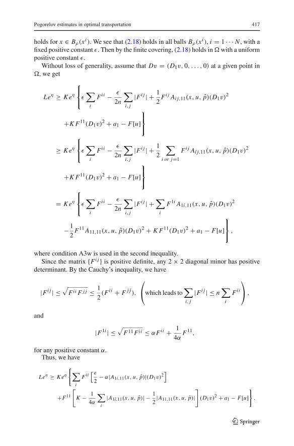
holds for x ∈ Bρ(xi ). We see that (2.18) holds in all balls Bρ(xi ), i = 1 · · · N , with afixed positive constant ε. Then by the finite covering, (2.18) holds in�with a uniformpositive constant ε.
Without loss of generality, assume that Dv = (D1v, 0, . . . , 0) at a given point in�, we get
Leη ≥ K eη
⎧⎨⎩ε∑
i
Fii − ε
2n
∑i, j
|Fi j | + 1
2Fi j Ai j,11(x, u, p)(D1v)2
+K F11(D1v)2 + a1 − F[u]⎫⎬⎭
≥ K eη
⎧⎨⎩ε∑
i
Fii − ε
2n
∑i, j
|Fi j | + 1
2
∑i or j=1
Fi j Ai j,11(x, u, p)(D1v)2
+K F11(D1v)2 + a1 − F[u]⎫⎬⎭
= K eη
⎧⎨⎩ε∑
i
Fii − ε
2n
∑i, j
|Fi j | +∑
i
F1i A1i,11(x, u, p)(D1v)2
−1
2F11A11,11(x, u, p)(D1v)2 + K F11(D1v)2 + a1 − F[u]
⎫⎬⎭ ,
where condition A3w is used in the second inequality.Since the matrix {Fi j } is positive definite, any 2 × 2 diagonal minor has positive
determinant. By the Cauchy’s inequality, we have
|Fi j | ≤√
Fii F j j ≤ 1
2(Fii + F j j ),
⎛⎝which leads to∑
i, j
|Fi j | ≤ n∑
i
Fii
⎞⎠ ,
and
|F1i | ≤√
F11Fii ≤ αFii + 1
4αF11,
for any positive constant α.Thus, we have
Leη ≥ K eη
{∑i
Fii[ ε2
− α|A1i,11(x, u, p)|(D1v)2]
+F11
[K − 1
4α
∑i
|A1i,11(x, u, p)| − 1
2|A11,11(x, u, p)|
](D1v)2 + a1 − F[u]
}.
123
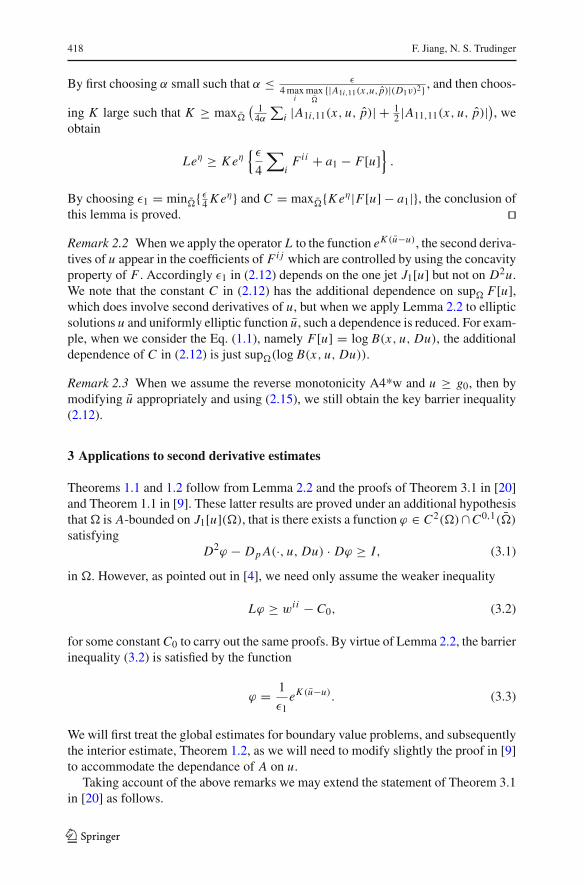
418 F. Jiang, N. S. Trudinger
By first choosing α small such that α ≤ ε4max
imax
�{|A1i,11(x,u, p)|(D1v)2} , and then choos-
ing K large such that K ≥ max�
( 14α
∑i |A1i,11(x, u, p)| + 1
2 |A11,11(x, u, p)|), weobtain
Leη ≥ K eη{ε
4
∑i
Fii + a1 − F[u]}
.
By choosing ε1 = min�{ ε4 K eη} and C = max�{K eη|F[u] − a1|}, the conclusion of
this lemma is proved. �Remark 2.2 Whenwe apply the operator L to the function eK (u−u), the second deriva-tives of u appear in the coefficients of Fi j which are controlled by using the concavityproperty of F . Accordingly ε1 in (2.12) depends on the one jet J1[u] but not on D2u.We note that the constant C in (2.12) has the additional dependence on sup� F[u],which does involve second derivatives of u, but when we apply Lemma 2.2 to ellipticsolutions u and uniformly elliptic function u, such a dependence is reduced. For exam-ple, when we consider the Eq. (1.1), namely F[u] = log B(x, u, Du), the additionaldependence of C in (2.12) is just sup�(log B(x, u, Du)).
Remark 2.3 When we assume the reverse monotonicity A4*w and u ≥ g0, then bymodifying u appropriately and using (2.15), we still obtain the key barrier inequality(2.12).
3 Applications to second derivative estimates
Theorems 1.1 and 1.2 follow from Lemma 2.2 and the proofs of Theorem 3.1 in [20]and Theorem 1.1 in [9]. These latter results are proved under an additional hypothesisthat� is A-bounded on J1[u](�), that is there exists a function ϕ ∈ C2(�)∩C0,1(�)
satisfyingD2ϕ − Dp A(·, u, Du) · Dϕ ≥ I, (3.1)
in �. However, as pointed out in [4], we need only assume the weaker inequality
Lϕ ≥ wi i − C0, (3.2)
for some constant C0 to carry out the same proofs. By virtue of Lemma 2.2, the barrierinequality (3.2) is satisfied by the function
ϕ = 1
ε1eK (u−u). (3.3)
We will first treat the global estimates for boundary value problems, and subsequentlythe interior estimate, Theorem 1.2, as we will need to modify slightly the proof in [9]to accommodate the dependance of A on u.
Taking account of the above remarks we may extend the statement of Theorem 3.1in [20] as follows.
123

Pogorelov estimates in optimal transportation 419
Lemma 3.1 Let u ∈ C4(�) ∩ C1,1(�) be an elliptic solution of Eq. (1.1) in � withA, B ∈ C2(U). Suppose that A is regular on J1 = J1[u](�), that is
Dpk pl Ai j (·, u, Du)ξiξ jηkηl ≥ 0 (3.4)
in �, for all ξ, η ∈ Rn such that ξ · η = 0, and that A satisfies (3.2) for some
ϕ ∈ C2(�) ∩ C0,1(�), with inf J1 B > 0. Then we have the estimate
sup�
|D2u| ≤ C
(1 + sup
∂�
|D2u|)
, (3.5)
where the constant C depends on A, B,�, |u|0,1;�, |ϕ|0,1;� and C0.
Clearly, Theorem 1.1 follows immediately from Lemmas 2.2 and 3.1. As an imme-diate consequence of Theorem 1.1, the hypothesis of the existence of a subsolution u inTheorem 1.1 of [4] can be removed altogether in the optimal transportation case, whilefor the Dirichlet problem in Theorem 1.2 of [4], we need only assume the existenceof a subsolution u in a neighbourhood of the boundary, whose boundary trace is theprescribed boundary function. However, the natural boundary condition for optimaltransportation and the more general prescribed Jacobian equations is the prescriptionof the image of the mapping, T u := Y (·, u, Du), that is
T u(�) = �∗ (3.6)
for some given target domain �∗ ∈ Y (U). Global estimates for solutions of Eq. (1.1)subject to (3.6) now follow from Theorem 1.1 under appropriate convexity hypotheseson � and �∗. As with (3.1) and (3.4), we will express these initially in terms of J1[u].Accordingly, we assume the domain� is uniformly A-convex with respect to J1[u] inthe sense that there exists a defining function ϕ ∈ C2(�) satisfying ϕ = 0, Dϕ �= 0on ∂� together with the “uniform convexity” condition (3.1) in a neighbourhoodN of∂�, while for the domain �∗ we assume the dual condition, that �∗ is uniformly Y ∗-convexwith respect to J1[u], namely that there exists a defining function ϕ∗ ∈ C2(�∗)satisfying ϕ∗ = 0, Dϕ∗ �= 0 on ∂�∗ together with the “dual uniform convexity”condition:
D2ϕ∗ − A∗i j,k(·, u, Du)Dkϕ
∗ ≥ I (3.7)
in a neighbourhood N ∗ of ∂�∗, where A∗i j,k is given by
[A∗i j,k] = Y −1
p DppY k(Y −1p )t (3.8)
for each k = 1, . . . , n. Taking account of (1.2) we see that these conditions canbe formulated for general prescribed Jacobian equations where Y ∈ C2(U) satisfiesdet Yp �= 0, and are not necessarily restricted to those determined through generatingfunctions. Furthermore, writing
G(x, u, p) = ϕ∗ ◦ Y (x, u, p), (3.9)
123
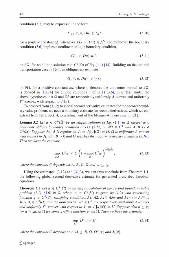
420 F. Jiang, N. S. Trudinger
condition (3.7) may be expressed in the form
G pp(x, u, Du) ≥ δ∗0 I (3.10)
for a positive constant δ∗0 , whenever Y (x, u, Du) ∈ N ∗ and moreover the boundary
condition (3.6) implies a nonlinear oblique boundary condition,
G(·, u, Du) = 0, (3.11)
on ∂�, for an elliptic solution u ∈ C2(�) of Eq. (1.1) [14]. Building on the optimaltransportation case in [20], an obliqueness estimate
G p(·, u, Du) · γ ≥ κ0 (3.12)
on ∂�, for a positive constant κ0, where γ denotes the unit outer normal to ∂�,is derived in [10,14] for elliptic solutions u of (1.1) (3.6), in C3(�), under theabove hypotheses that � and �∗ are respectively uniformly A-convex and uniformlyY ∗-convex with respect to J1[u].
To proceed from (3.12) to global second derivative estimates for the second bound-ary value problem, we need a boundary estimate for second derivatives, which we canextract from [20], Sect. 4, as a refinement of the Monge–Ampère case in [21].
Lemma 3.2 Let u ∈ C4(�) be an elliptic solution of Eq. (1.1) in � subject to anonlinear oblique boundary condition (3.11), (3.12) on ∂� ∈ C4 with A, B, G ∈C2(U). Suppose that A is regular on J1 = J1[u](�) � U , � is uniformly A-convexwith respect to J1, inf J1B > 0 and G satisfies the uniform convexity condition (3.10).Then we have the estimate,
sup∂�
|D2u| ≤ C
(1 + sup
�
|D2u|) 2n−3
2(n−1)
, (3.13)
where the constant C depends on A, B, G,� and |u|0,1;�.
Using the estimates, (3.12) and (3.13), we can thus conclude from Theorem 1.1,the following global second derivative estimate for generated prescribed Jacobianequations.
Theorem 3.1 Let u ∈ C4(�) be an elliptic solution of the second boundary valueproblem (1.1), (3.6) in �, where A ∈ C2(U) is given by (1.2) with generatingfunction g ∈ C4(�), satisfying conditions A1, A2, A1*, A3w and A4w (or A4*w),B > 0,∈ C2(U) and the domains �,�∗ ∈ C4 are respectively uniformly A-convexand uniformly Y ∗-convex with respect to J1 = J1[u](�) � U . Suppose also u ≤ g0(or u ≥ g0) in � for some g-affine function g0 on �. Then we have the estimate,
sup�
|D2u| ≤ C, (3.14)
where the constant C depends on n,U , g, B,�,�∗, g0 and J1[u].
123

Pogorelov estimates in optimal transportation 421
We may express the domain convexity hypotheses in Theorem 3.1 in terms ofboundary data depending on the solution u or more specifically, as in [10], intervalscontaining the range of u. For this purpose we will say that � is uniformly Y -convexwith respect to (�∗, u) if
(Diγ j − Dp Ai j (x, u(x), p) · Dγ )τiτ j ≥ δ0, (3.15)
for all x ∈ ∂�, Y (x, u(x), p) ∈ �∗, unit outer normal γ and unit tangent vector τ , forsome constant δ0 > 0. Similarly the target domain �∗ is uniformly Y ∗-convex withrespect to (�, u) if
[Diγ
∗j (y) − A∗
i j,k(x, u(x), p)γ ∗k (y)
]τiτ j ≥ δ∗
0 , (3.16)
for all x ∈ �, y = Y (x, u(x), p) ∈ ∂�∗, unit outer normal γ ∗ and unit tangent vectorτ , for some constant δ∗
0 > 0. It then follows that the uniform convexity assumptions inTheorem 3.1 may be replaced by �, �∗ being respectively uniformly Y -convex, Y ∗-convex with respect to (�∗, u), (�, u). Moreover these assumptions are equivalent tothe convexity notions defined in terms of the generating function g in [16]. Assuming� and �∗ are connected and T u is a diffeomorphism, then � is uniformly Y -convexwith respect to (�∗, u) if and only if � is uniformly g-convex with respect to v, thatis the images Q(·, y, v(y))(�) are uniformly convex for all y ∈ �∗, where v is theg-transform of u on �∗, given by
v(y) = g∗(x, y, u(x)) = Z(x, u(x), Du(x)), (3.17)
for y = T u(x), while �∗ is uniformly Y ∗-convex with respect to (�, u) if and onlyif �∗ is uniformly g∗-convex with respect to u, that is the images P(x, ·, u(x))(�∗)are uniformly convex for all x ∈ �, where P(x, y, u) = gx (x, y, g∗(x, y, u)) for(x, y, u) ∈ �∗; see [16] for more details.
Returning to the Dirichlet problem, we state the following analogue of Theorem3.1, which follows from Theorem 1.1 and our boundary estimates in [4].
Theorem 3.2 Let u ∈ C4(�) be an elliptic solution of (1.1) in �, satisfying u = u0 on∂�, where A ∈ C2(U) is given by (1.2) with generating function g ∈ C4(�), satisfyingconditions A1, A2, A1*, A3w and A4w (or A4*w), B > 0,∈ C2(U), u0 ∈ C4(�) andthe domain � ∈ C4 is uniformly A-convex with respect to J1 = J1[u](�) � U .Suppose also u ≤ g0 (or u ≥ g0) in � for some g-affine function g0 on �. Then wehave the estimate,
sup�
|D2u| ≤ C, (3.18)
where the constant C depends on n,U , g, B,�, ϕ, g0 and J1[u].To reduce the proof of Theorem 3.2 to our boundary estimates in Section 3 of [4],
we replace u by u0 in inequality (3.5) there and use the barrier v = −Cϕ in placeof v = 1 − φ, for sufficiently large constant C , in the rest of the proof, where ϕ isa defining function in the definition of A-convexity. Note that under the assumption
123

422 F. Jiang, N. S. Trudinger
of uniform A-convexity we do not need Lemma 2.2 to obtain the second derivativeboundary estimate, which is already asserted in [13]. Note also that in these argumentsthe dependence of the coefficients on u can be removed by replacing u by u(x).
To conclude this sectionwe indicate howTheorem 1.2 follows fromLemma 2.2 and[9]. In the optimal transportation case (1.3), when A is independent of u, we simplyuse (3.3) in the proof of Theorem 1.1 in [9] instead of (3.1), with u0 replaced by g0. Inthe general case we proceed the same way, first noting that the monotonicity conditionA4w ensures η = g0 −u > 0 in �, by virtue of the strong maximum principle [2] andthe fact that g0 is a degenerate elliptic solution of the homogeneous equation, (B = 0).We then consider as in [9], the corresponding auxiliary function
v = τ log η + log(wi jξiξ j ) + 1
2β|Du|2 + eκϕ, (3.19)
where β, κ, τ are positive constants to be determined and estimate Lv from below atan interior maximum point x = x , where
Lv = Lv − Dp(log B)·Dv.
As in Section 3 of [20], the additional terms arising from the the u dependence, in thedifferentiations of (1.1), are absorbed in the lower bounds (18) and (19) in [9] so itremains to extend the lower bound for Lη in inequalities (20) and (21) in [9], wherenow η = g0 − u. This is done similarly to the argument in the proof of Lemma 2.2,as follows. By calculation, we have
Lη = wi j [Di jη − Dpk Ai j (x, u, Du)Dkη] − Dpk (log B)Dkη
= wi j [−wi j + Ai j (x, g0, Dg0) − Ai j (x, u, Du) − Dpk Ai j (x, u, Du)Dkη]−Dpk (log B)Dkη
≥ −C + wi j [Ai j (x, g0, Dg0) − Ai j (x, u, Du) − Dpk Ai j (x, u, Du)Dkη]≥ −C + wi j [Ai j (x, u, Dg0) − Ai j (x, u, Du) − Dpk Ai j (x, u, Du)Dkη]= −C + 1
2wi j Ai j,kl(x, u, p)DkηDlη, (3.20)
where p = (1 − θ)Dg0 + θ Du for some θ ∈ (0, 1), condition A4w is used in thesecond inequality and Taylor’s formula is used in the last equality. By assuming {wi j }is diagonal, we have from (3.20)
Lη ≥ −Cn + 1
2wi i Aii,kl(x, u, p)DkηDlη,
≥ −C +∑k �=i
wi i Aii,ik(x, u, p)DiηDkη + 1
2wi i Aii,i i (x, u, p)(Diη)2
≥ −C(1 + wi i |Diη|), (3.21)
where condition A3w is used in the second inequality and the constant C depends on�, A, B, g0 and J1[u]. We remark that the particular form of the estimate (3.21) isactually crucial in the ensuing estimations in [9].
123

Pogorelov estimates in optimal transportation 423
Accordingly we obtain from [9], an estimate,
(g0 − u)τ |D2u| ≤ C (3.22)
for positive constants τ and C , corresponding to the estimate (9) in [9]. Our desiredestimate (1.5) follows, noting also that the estimate (28) in [9] for u0 − u from belowextends automatically when we substitute u(x) for u in A and B.
4 Optimal transportation and geometric optics
4.1 Optimal transportation
For our applications to optimal transportation when g reduces to a cost function cthrough (1.3), it will suffice to assume c ∈ C4(� × �∗) where the domains � and�∗ are respectively uniformly c and c∗-convex with respect to each other, that is theimages cy(·, y)(�) and cx (x, ·)(�∗) are uniformly convex in R
n , for each y ∈ �∗,x ∈ �.
Conditions A1, A1*, A2 and A3w can then be written as:
A1: The mappings cx (x, ·), cy(·, y) are one-to-one for each x ∈ �, y ∈ �∗;A2: det cx,y �= 0 in � × �∗;A3w: (Dpk pl Ai j (x, p))ξiξ jηkηl ≥ 0, for all (x, p) ∈ �×R
n such that Y (x, p) ∈�∗ and ξ, η ∈ R
n such that ξ ·η = 0.
Here we also have the simpler formulae,
Y (x, u, p) = Y (x, p) = c−1x (x, ·)(p), A(x, u, p) = A(x, p) = cxx (x, Y ). (4.1)
We then conclude from Theorem 3.2 the following global second derivative estimatewhich improves Theorem 1.1 in [20] and Theorem 2.1 in [15].
Corollary 4.1 Let u ∈ C4(�) be an elliptic solution of the second boundary valueproblem (1.1), (3.6) in �, where A is given by (4.1) with cost function c satisfyingconditions A1, A2 and A3w and B > 0,∈ C2( J1[u]) and the domains �,�∗ ∈ C4 arerespectively uniformly c-convex and uniformly c∗-convex with respect to each other.Then we have the estimate,
sup�
|D2u| ≤ C, (4.2)
where the constant C depends on n, c, B,�,�∗ and J1[u].For application to optimal transportation, the function B has the form
B(·, u, p) = | det cx,y |ρρ∗ ◦ Y (·, p)
(4.3)
where ρ and ρ∗ are positive densities defined on � and �∗ respectively, satisfying themass balance condition ∫
�
ρ =∫
�∗ρ∗, (4.4)
123

424 F. Jiang, N. S. Trudinger
which is a necessary condition for a solution u for which the mapping Tu = Y (·, Du)
is a diffeomorphism. From Corollary 4.1, we obtain following [20] the existence of anelliptic solution u ∈ C3(�) which is unique up to additive constants, as formulated inTheorem 1.1 in [15]. However our proof of Corollary 4.1 in this case is more direct andmore general than the approach in [15] which depends on a strict convexity regularityresult of Figalli et al. [1]. From the existence we obtain the existence of a smoothoptimal mapping solving the transportation problem as formulated in Corollary 1.2 in[15].
Examples of cost functions which satisfy condition A3w and not A3 are givenin [20] and [9]. However for these examples the global second derivative bounds inTheorems 1.1 and 4.1 are proved in [20] from other structures such as c-boundednessor duality so that Corollary 4.1 is not new in these cases. This is not the case thoughfor the interior estimate, Theorem 1.2, which for example is new for the cost functionc(x, y) = |x − y|−2. For explicit calculations in this case the reader is referred to [8],as well as [20].
4.2 Geometric optics
Keeping to domains in Euclidean space, we will just consider here parallel beams inR
n+1, directed in the en+1 direction, through a domain � ⊂ Rn × {0}, illuminating
targetswhich are graphs over domains�∗ inRn ×{0}. The formulae are easily adjustedto cover more general situations and we may also consider point sources of light asin [6]. The special cases where the targets are themselves domains in R
n × {0} yieldstrictly regular matrix functions A and global estimates for the second boundary valueproblem are already proved in [10,14]. Consequently our main interest here is withsituations where the resultant matrices A satisfy A3w and not necessarily A3, althoughas we indicated in Sect. 1 our lemmas in Sect. 2 are still new in this case.
(i) Reflection. We modify slightly the example in [16] to allow for non-flat targets;see also [7] for a thorough description of the geometric picture.Let D be a domain in Rn ×R
n , containing � × �∗, and consider the generatingfunction:
g(x, y, z) = �(y) + 1
2z− z
2|x − y|2, (4.5)
defined for (x, y) ∈ D and z > 0 where � is a smooth function on Rn . By
differentiation we havegx (x, y, z) = z(y − x) (4.6)
so that if there are mappings y = Y (x, u, p), z = Z(x, u, p) satisfying A1, wemust have y = x + p/z and from (4.5),
u = h(z) = �
(x + p
z
)+ 1
2z
(1 − |p|2
). (4.7)
123

Pogorelov estimates in optimal transportation 425
By differentiation we then obtain,
h′(z) = − 1
2z2(2p ·D� + 1 − |p|2) < 0, (4.8)
provided
2p ·D� + 1 − |p|2 > 0,
that is,z2|y − x |2 + 2z(x − y)·D� − 1 < 0. (4.9)
Accordingly conditions A1 and A2 will be satisfied for 0 < z < z0(x, y), where
z0 = 1√|x − y|2 + |(x − y)·D�|2 + (x − y)·D�, (4.10)
Y (x, u, p) = x + p/Z(x, u, p) and Z , given implicitly by (4.7), satisfies Zu < 0.Now from (4.6), we see that the matrix A is given by
A(x, u, p) = −Z(x, u, p)I (4.11)
and hence conditions A3w and A4w are both satisfied whenever the dual functionZ is concave in the gradient variables. It also follows that condition A1* is alsosatisfied when (4.9) holds, that is the mapping Q given by
Q(x, y, z) = 2z2D� + z(x − y)
1 + z2|x − y|2
is one to one in x , for 0 < z < z0(x, y), which can be proved for example fromthe quadratic structure of the equation, Q(x, y, z) = q. Furthermore by taking zsufficiently small, we see that there exist arbitrarily large g-affine functions andhence all the hypotheses of Theorems 1.1 and 1.2 are satisfied by the generatingfunction g if Z is concave in p. Note that when � is constant, then Z = (1 −|p|2)/2(u −�), u > �, |p| < 1 and the strict condition A3 holds, [16]. By directcalculation, we have an explicit formula for the matrix E ,
E = z
{I − 2z(x − y) ⊗ [z(x − y) + D�]
1 + z2|x − y|2}
,
and its determinant
det E = −zn z2|x − y|2 + 2z(x − y)·D� − 1
1 + z2|x − y|2 > 0,
123

426 F. Jiang, N. S. Trudinger
when (4.9) holds. By the Sherman–Morrison formula, we also have a formula forthe inverse of E ,
E−1 = 1
z
{I − 2z(x − y) ⊗ [z(x − y) + D�]
z2|x − y|2 + 2z(x − y)·D� − 1
}.
(ii) Refraction. We consider refraction from media I to media II with respectiverefraction indices n1, n2 > 0 and set κ = n1/n2. For κ �= 1, we consider nowgenerating functions,
g(x, y, z) = �(y) − 1
|κ2 − 1|(
κz +√
z2 + (κ2 − 1)|x − y|2)
, (4.12)
where again (x, y) ∈ D, z >√1 − κ2|x − y| for 0 < κ < 1, > 0 for κ > 1 and
� is a smooth function on Rn . For more details about the geometric and physicalaspects of this model, see for example [12]. We will now restrict attention to thecase 0 < κ < 1, in which case by setting κ ′ = √
1 − κ2 and rescaling z → z/κ ′,� → κ ′�, g → κ ′g, we can write
g(x, y, z) = �(y) − κz −√
z2 − |x − y|2. (4.13)
By differentiation we now have
gx (x, y, z) = x − y√z2 − |x − y|2 (4.14)
so that if there are mappings y = Y (x, u, p), z = Z(x, u, p) satisfying A1, wemust have
y = x − zp√1 + |p|2 ,
so from (4.13),
u = h(z) = �
(x − zp√
1 + |p|2)
− κz − z√1 + |p|2 . (4.15)
By differentiation we then obtain,
h′(z) = − 1√1 + |p|2
(p ·D� + 1 + κ
√1 + |p|2
)< 0, (4.16)
provided
p ·D� + 1 + κ
√1 + |p|2 > 0,
123
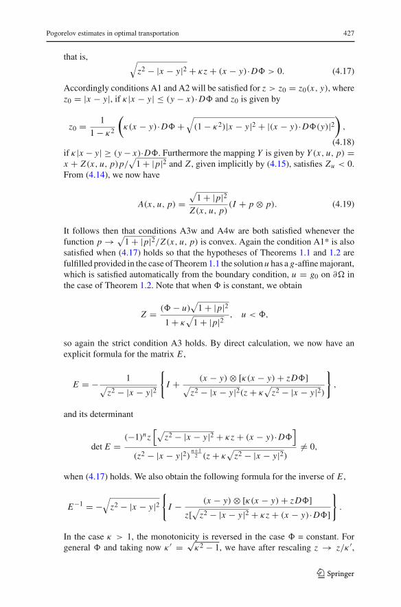
Pogorelov estimates in optimal transportation 427
that is, √z2 − |x − y|2 + κz + (x − y)·D� > 0. (4.17)
Accordingly conditions A1 and A2 will be satisfied for z > z0 = z0(x, y), wherez0 = |x − y|, if κ|x − y| ≤ (y − x)·D� and z0 is given by
z0 = 1
1 − κ2
(κ(x − y)·D� +
√(1 − κ2)|x − y|2 + |(x − y)·D�(y)|2
),
(4.18)if κ|x − y| ≥ (y − x)·D�. Furthermore the mapping Y is given by Y (x, u, p) =x + Z(x, u, p)p/
√1 + |p|2 and Z , given implicitly by (4.15), satisfies Zu < 0.
From (4.14), we now have
A(x, u, p) =√1 + |p|2
Z(x, u, p)(I + p ⊗ p). (4.19)
It follows then that conditions A3w and A4w are both satisfied whenever thefunction p → √
1 + |p|2/Z(x, u, p) is convex. Again the condition A1* is alsosatisfied when (4.17) holds so that the hypotheses of Theorems 1.1 and 1.2 arefulfilled provided in the case ofTheorem1.1 the solution u has a g-affinemajorant,which is satisfied automatically from the boundary condition, u = g0 on ∂� inthe case of Theorem 1.2. Note that when � is constant, we obtain
Z = (� − u)√1 + |p|2
1 + κ√1 + |p|2 , u < �,
so again the strict condition A3 holds. By direct calculation, we now have anexplicit formula for the matrix E ,
E = − 1√z2 − |x − y|2
{I + (x − y) ⊗ [κ(x − y) + zD�]√
z2 − |x − y|2(z + κ√
z2 − |x − y|2)
},
and its determinant
det E =(−1)nz
[√z2 − |x − y|2 + κz + (x − y)·D�
]
(z2 − |x − y|2) n+12 (z + κ
√z2 − |x − y|2)
�= 0,
when (4.17) holds. We also obtain the following formula for the inverse of E ,
E−1 = −√
z2 − |x − y|2{
I − (x − y) ⊗ [κ(x − y) + zD�]z[√z2 − |x − y|2 + κz + (x − y)·D�]
}.
In the case κ > 1, the monotonicity is reversed in the case � = constant. Forgeneral � and taking now κ ′ = √
κ2 − 1, we have after rescaling z → z/κ ′,
123
428 F. Jiang, N. S. Trudinger
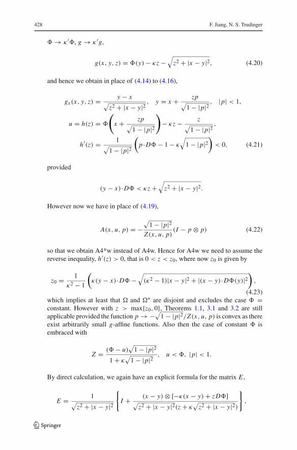
� → κ ′�, g → κ ′g,
g(x, y, z) = �(y) − κz −√
z2 + |x − y|2, (4.20)
and hence we obtain in place of (4.14) to (4.16),
gx (x, y, z) = y − x√z2 + |x − y|2 , y = x + zp√
1 − |p|2 , |p| < 1,
u = h(z) = �
(x + zp√
1 − |p|2)
− κz − z√1 − |p|2 ,
h′(z) = 1√1 − |p|2
(p ·D� − 1 − κ
√1 − |p|2
)< 0, (4.21)
provided
(y − x)·D� < κz +√
z2 + |x − y|2.
However now we have in place of (4.19),
A(x, u, p) = −√1 − |p|2
Z(x, u, p)(I − p ⊗ p) (4.22)
so that we obtain A4*w instead of A4w. Hence for A4w we need to assume thereverse inequality, h′(z) > 0, that is 0 < z < z0, where now z0 is given by
z0 = 1
κ2 − 1
(κ(y − x)·D� −
√(κ2 − 1)|x − y|2 + |(x − y)·D�(y)|2
),
(4.23)which implies at least that � and �∗ are disjoint and excludes the case � =constant. However with z > max{z0, 0}, Theorems 1.1, 3.1 and 3.2 are stillapplicable provided the function p → −√1 − |p|2/Z(x, u, p) is convex as thereexist arbitrarily small g-affine functions. Also then the case of constant � isembraced with
Z = (� − u)√1 − |p|2
1 + κ√1 − |p|2 , u < �, |p| < 1.
By direct calculation, we again have an explicit formula for the matrix E ,
E = 1√z2 + |x − y|2
{I + (x − y) ⊗ [−κ(x − y) + zD�]√
z2 + |x − y|2(z + κ√
z2 + |x − y|2)
},
123

Pogorelov estimates in optimal transportation 429
and its determinant
det E = z[√z2 + |x − y|2 + κz + (x − y)·D�](z2 + |x − y|2) n+1
2 (z + κ√
z2 + |x − y|2)�= 0,
when h′(z) �= 0. By the Sherman-Morrison formula, we also obtain the inverseof E ,
E−1 =√
z2 + |x − y|2{
I − (x − y) ⊗ [−κ(x − y) + zD�]z[√z2 + |x − y|2 + κz + (x − y)·D�]
}.
As in the previous cases the condition A1* will hold if either h′(z) < 0, (thatis det E > 0), or h′(z) > 0, (that is det E < 0), which again follows from theequivalent quadratic structure of the equation Q(x, y, z) = q.
(iii) Further remarks. It is interesting to note that when we pass to the dual functionsin the above examples the monotonicity of A is reversed but, as shown in generalin [16], the condition A3w is preserved. In particular for the dual in the reflectioncase (4.5) we have from [16],
g∗(x, y, u) = 1
u − �(y) +√(u − �(y))2 + |x − y|2 , (4.24)
while in the refraction cases (4.12), a simple calculation gives
g∗(x, y, u) = +, (−)
(κ(u − �(y)) +
√(u − �(y))2 + |x − y|2
), (4.25)
for κ < 1, (κ > 1) respectively. Note that by replacing z by −1/z in (4.5), thedual function in (4.24) is the limit as κ → 1 of the case κ > 1 in (4.25).
Alsowenote thatwhenweconsider instead the complementary ellipticity condition,D2u − A(·, u, Du) < 0, in Eq. (1.1), condition A3w is replaced by substituting −Afor A but conditions A4w and A4*w are maintained. Thus in the above examples weneed to replace Z by−Z in the convexity conditions, (and interchange the inequalitiesu < g0, u > g0), to fulfil our hypotheses.
As well as the monotonicity properties, another interesting ingredient of the aboveexamples is that we cannot infer, as in the optimal transportation examples mentionedin the previous section, that bounded domains are A-bounded so second derivativeestimates do not follow from the relevant arguments in [14,20].
4.3 Final remarks
The existence of locally smooth solutions to the second boundary value problem forgenerated prescribed Jacobian equations is treated in [16] under conditions A1, A2,A1*, A3 and A4w. We remark that there that the montonicity condition A4w may
123

430 F. Jiang, N. S. Trudinger
also be replaced by condition A4* for local regularity. In [17] and ensuing work themonotonicity condition A4w is relaxed and local boundary regularity is also consid-ered, yielding an alternative approach to that in [10] which deals with estimates andexistence of globally smooth solutions. We remark that the strict monotonicity of Z ,in our examples in Sect. 4.2, also follows from a general formula in [17],
Zu = det gx,y
gz det E.
In a follow up work [3] we will use our estimates here to extend the global theorywhen A3 is weakened to A3w, without A-boundedness conditions, as well as furtherdevelop the optics examples.We also develop an alternative duality approach to secondderivative estimates when the matrix A depends only on u and p. As already noted in[20], this situation is much simpler in two dimensions.
Finally we wish to thank the anonymous referee of this paper for their carefulchecking and useful comments.
Open Access This article is distributed under the terms of the Creative Commons Attribution Licensewhich permits any use, distribution, and reproduction in any medium, provided the original author(s) andthe source are credited.
References
1. Figalli, A., Kim, Y.-H., McCann, R.J.: Hölder continuity and injectivity of optimal maps. Arch. Ration.Mech. Anal. 209, 747–795 (2013)
2. Gilbarg, D., Trudinger, N.S.: Elliptic Partial Differential Equation of Second Order. Springer, Berlin(2001)
3. Jiang, F., Trudinger, N.S.: On the second boundary value problem for Monge–Ampère type equationsand geometric optics (in preparation)
4. Jiang, F., Trudinger, N.S., Yang, X.-P.: On the Dirichlet problem for Monge–Ampère type equations.Calc. Var. Partial Differ. Equ. 49, 1223–1236 (2014)
5. Jiang, F., Trudinger, N.S., Yang, X.-P.: On the Dirichlet problem for a class of augmented Hessianequations. Preprint (2014)
6. Karakhanyan, A., Wang, X.-J.: On the reflector shape design. J. Differ. Geom. 84, 561–610 (2010)7. Karakhanyan, A.: Existence and regularity of the reflector surfaces inRn+1. Arch. Ration.Mech. Anal.
213, 833–885 (2014)8. Kim, Y.-H., Kitagawa, J.: On the degeneracy of optimal transportation. Commun. Partial Differ. Equ.
39, 1329–1363 (2014)9. Liu, J., Trudinger, N.S.: On Pogorelov estimates for Monge–Ampère type equations. Discret. Contin.
Dyn. Syst. Ser. A. 28, 1121–1135 (2010)10. Liu, J., Trudinger, N.S.: On classical solutions of near field reflection problems. Preprint (2014)11. Ma, X.-N., Trudinger, N.S.,Wang, X.-J.: Regularity of potential functions of the optimal transportation
problem. Arch. Ration. Mech. Anal. 177, 151–183 (2005)12. Oliker, V.: Differential equations for design of a freeform single lens with prescribed irradiance prop-
erties. Opt. Eng. 53, 031302–1-10 (2014)13. Trudinger, N.S.: Recent developments in elliptic partial differential equations of Monge–Ampère type.
ICM. Madr. 3, 291–302 (2006)14. Trudinger, N.S.: On the prescribed Jacobian equation. In: Proceedings of International Conference for
the 25th Anniversary of Viscosity Solutions, Gakuto International Series.Math. Sci. Appl. 20, 243–255(2008)
123

Pogorelov estimates in optimal transportation 431
15. Trudinger, N.S.: A note on global regularity in optimal transportation. Bull. Math. Sci. 3, 551–557(2013)
16. Trudinger, N.S.: On the local theory of prescribed Jacobian equations. Discret. Contin. Dyn. Syst. 34,1663–1681 (2014)
17. Trudinger, N.S.: On the local theory of prescribed Jacobian equations revisited (in preparation) (2014)18. Trudinger, N.S., Wang, X.-J.: The Monge–Ampère equation and its geometric applications. In: Hand-
book of geometric analysis. No. 1, Adv. Lect. Math. (ALM), vol. 7, pp. 467–524. International Press,Somerville (2008)
19. Trudinger, N.S.,Wang, X.-J.: On strict convexity and continuous differentiability of potential functionsin optimal transportation. Arch. Ration. Mech. Anal. 192, 403–418 (2009)
20. Trudinger, N.S., Wang, X.-J.: On the second boundary value problem for Monge–Ampère type equa-tions and optimal transportation. Ann. Scuola Norm. Sup. Pisa Cl. Sci. VIII, 143–174 (2009)
21. Urbas, J.: Oblique boundary value problems for equations of Monge–Ampère type. Calc. Var. PartialDiffer. Equ. 7, 19–39 (1998)
123