Embed Size (px)
Citation preview

On Partitioned Simulation of Electrical
Circuits using Dynamic Iteration Methods
vorgelegt von
Dipl.-Math.techn. Falk Ebert
von der Fakultat II - Mathematik und Naturwissenschaften
der Technischen Universitat Berlin
zur Erlangung des akademischen Grades
Doktor der Naturwissenschaften
- Dr. rer. nat. -
genehmigte Dissertation
Promotionsausschuss:
Vorsitzender: Prof. Dr. Gunter Ziegler
Berichter: Dr. Tatjana Stykel
Berichter: Prof. Dr. Volker Mehrmann
Berichter: Prof. Dr. Caren Tischendorf
Tag der wissenschaftlichen Aussprache: 08. September 2008
Berlin 2008
D 83

ii

Acknowledgment
... to my child ...
During the four years, that the work on this thesis took, countless people have con-tributed small or large parts to the final result. I will try to name those that crossmy mind and I beg the pardon of those that I miss here.My foremost gratitude goes to my advisor Dr. Tatjana Stykel who critically andpatiently supervised my work, who left me enormous freedom but still brought meback on track when I was straying too far from the actual subject and whom Igreatly esteem as a scientist and as a friend. I would like to thank Prof. Dr. VolkerMehrmann for his support and advise, for an always open door, for fruitful dis-cussions, helpful remarks and at all times one or two ideas of what could still beincluded. My thanks also go to Prof. Dr. Caren Tischendorf who was the one whointroduced me to electrical circuits and, thus, laid the basis for this thesis.I want to thank my colleagues of the research field Numerical Analysis at the Tech-nical University of Berlin for creating such an extraordinary and unique workingatmosphere. Especially, I want to express my gratitude to Drs. Christian Mehland Andreas Steinbrecher for their encouragement, well-meant criticism and theirpatience with my notation while proofreading this thesis. I am eternally indebtedto Dr. Steinbrecher for leaving behind the greatest office space in the whole mathe-matics building. My thanks also go to Drs. Simone Bachle, Sonja Schlauch, KathrinSchreiber, Michael Schmidt, Timo Reis and Christian Schroder and to Lisa Poppefor hints and discussions or simply for an open ear or two.I want to thank the people from the Combinatorial Optimization and Graph Algo-rithms group of Prof. Dr. Rolf Mohring. Especially, I want to thank Drs. ChristianLiebchen and Gregor Wunsch as well as Sebastian Stiller and Jens Schulz for intro-ducing me to graph theory.I am grateful to the DFG financed research center Matheon for providing such aninterdisciplinary research environment and for funding the project that this thesiswas created in. The examples part of this thesis would surely be less interestingif it were not for Markus Brunk who created a working diode simulator for use inthis work. In the same context, I want to thank Angelika Tobisch for introducingme to the chaotic beauty of Perl and Eva Abram who helped with lots of nastyimplementation details.I have to thank my friends and family for their support. Especially, I want to thankmy father Dr. Frank Ebert for his incessant optimism and encouragement.But I want to express my most heartfelt thanks to my wife Kristina Ebert forher love and warmth, for her smiles and comfort, for her patience and guidance,for putting up with me in all those years and for bestowing upon me someone todedicate this thesis to.
iii

iv

Eidesstattliche Versicherung
Hiermit erklare ich, dass ich die vorliegende Dissertationsschrift selbststandig ver-fasst habe und keine anderen als die in ihr angegebenen Quellen und Hilfsmittelbenutzt worden sind.
Berlin, den 08.07.2008 Falk Ebert
v

vi
Zusammenfassung
Im Rahmen dieser Arbeit wird die partitionierte Simulation elektrischer Schaltkreiseuntersucht. Hierbei handelt es sich um eine Technik, verschiedene Teile einesSchaltkreises auf unterschiedliche Weise numerisch zu behandeln um eine Simulationfur den Gesamtkreis zu erhalten. Dabei wird besonderes Augenmerk auf zwei Dingegelegt. Zum einen sollen samtliche analytischen Resultate eine graphentheoretischeInterpretation zulassen. Diese Bedingung resultiert daraus, dass Schaltkreisglei-chungen haufig sehr hochdimensional und schlecht skaliert sind und eine Behandlungmit Standardmethoden der linearen Algebra sehr schwierig wird. Die zweite Be-dingung ist, dass die erarbeiteten Methoden so formuliert werden, dass sie leicht inexistierende Software zur Schaltungssimulation integriert werden konnen. In dieserArbeit wird der weitverbreitete Schaltkreissimulator SPICE als Referenzprogrammverwendet.Zunachst werden die benotigten Grundlagen aus der Theorie der differentiell-alge-braischen Gleichungen, der Graphentheorie und der Schaltungssimulation vorge-stellt. Anschließend wird die Methode der dynamischen Iteration als Mittel zurgekoppelten Simulation partitionierter dynamischer Systeme prasentiert. Dabeiwird insbesondere auf die fundamentalen Unterschiede im Konvergenzverhaltenzwischen gewohnlichen Differentialgleichungen und differentiell-algebraischen Glei-chungen eingegangen. Es werden hinreichende Konvergenzkriterien fur den Fallallgemeiner gekoppelter differentiell-algebraischer Gleichungen erortert und diesedann fur semi-explizite Systeme spezifiziert. Desweiteren werden fur diese Systememodifizierte dynamische Iterationsverfahren vorgeschlagen, welche die Konvergenzdes Verfahrens erzwingen und beschleunigen konnen.Anschließend werden die erbrachten Resultate auf den Spezialfall von partitioniertenSchaltungsgleichungen angewandt. Dazu wird zuerst eine Methode vorgestellt,die es ermoglicht, die Schaltkreisgleichungen so zu partitionieren, dass eine ele-mentspezifische Trennung moglich ist und die entstehenden Teilsysteme weiterhinals Schaltkreise interpretiert werden konnen. Fur die Klasse von partitioniertenWiderstandsnetzwerken wurden Konvergenzkriterien hergeleitet, die zu großen Tei-len auf graphentheoretischen Uberlegungen basieren. Desweiteren werden die zuvorvorgestellten Methoden zur Konvergenzbeschleunigung erfolgreich auf Schaltkreiseangewandt. Dabei konnen samtliche notwendigen Gleichungstransformationen alsModifikationen des Schaltkreises selbst interpretiert werden. Die erhaltenen Re-sultate fur Widerstandsnetzwerke werden dann auf den Fall von partitioniertenRCL-Schaltkreisen verallgemeinert.Nach diesen analytischen Betrachtungen werden die Aspekte der numerischen Durch-fuhrung von dynamischen Iterationsverfahren erortert. Dabei wird ein erweitertesKonvergenzkriterium vorgestellt, welches die bei der approximativen Losung vondynamischen Systemen auftretenden Fehler mit einbezieht. Desweiteren wird derEinfluss von Makroschrittweiten auf die Effizienz des dynamischen Iterationsver-fahrens erlautert und eine einfache Schrittweitensteuerung vorgeschlagen.Abschließend werden die gewonnenen theoretischen Erkenntnisse anhand von vierBeispielen verifiziert.
vii

viii

Contents
1 Introduction 3
2 Preliminaries 7
2.1 Some results from Linear Algebra . . . . . . . . . . . . . . . . . . . . 7
2.2 Some results from Analysis . . . . . . . . . . . . . . . . . . . . . . . 13
2.3 Differential-Algebraic Equations . . . . . . . . . . . . . . . . . . . . . 17
2.4 Basic Graph Theory . . . . . . . . . . . . . . . . . . . . . . . . . . . 21
2.4.1 Basic structures . . . . . . . . . . . . . . . . . . . . . . . . . 21
2.4.2 Graph related matrices . . . . . . . . . . . . . . . . . . . . . 24
2.5 Basic Circuit Theory . . . . . . . . . . . . . . . . . . . . . . . . . . . 28
2.5.1 Elements of lumped circuit simulation . . . . . . . . . . . . . 28
2.5.2 Modified Nodal Analysis . . . . . . . . . . . . . . . . . . . . . 32
2.5.3 The matrices Y∗ and Z∗ . . . . . . . . . . . . . . . . . . . . . 34
2.5.4 Index and topology . . . . . . . . . . . . . . . . . . . . . . . . 36
3 Dynamic Iteration Methods 41
3.1 Dynamic Iteration for ODEs . . . . . . . . . . . . . . . . . . . . . . . 41
3.2 Dynamic Iteration for DAEs . . . . . . . . . . . . . . . . . . . . . . . 43
3.3 Gauss-Seidel and Jacobi methods . . . . . . . . . . . . . . . . . . . . 54
3.4 Conclusion . . . . . . . . . . . . . . . . . . . . . . . . . . . . . . . . 73
4 DIM in circuit simulation 75
4.1 Previous results . . . . . . . . . . . . . . . . . . . . . . . . . . . . . . 75
4.2 List of variables . . . . . . . . . . . . . . . . . . . . . . . . . . . . . . 77
4.3 General splitting approach . . . . . . . . . . . . . . . . . . . . . . . . 79
4.3.1 The purely resistive case . . . . . . . . . . . . . . . . . . . . . 88
4.3.2 The RCL case . . . . . . . . . . . . . . . . . . . . . . . . . . 101
4.4 Topological acceleration of convergence . . . . . . . . . . . . . . . . . 122
4.4.1 The purely resistive case . . . . . . . . . . . . . . . . . . . . . 123
4.4.2 The RCL case . . . . . . . . . . . . . . . . . . . . . . . . . . 132
4.5 A note on the index of MNA equations in DIMs . . . . . . . . . . . . 134
4.6 Conclusion . . . . . . . . . . . . . . . . . . . . . . . . . . . . . . . . 138
5 Numerical Aspects of Dynamic Iteration Methods 139
5.1 Numerical solution of DAEs . . . . . . . . . . . . . . . . . . . . . . . 139
5.1.1 BDF methods . . . . . . . . . . . . . . . . . . . . . . . . . . . 140
5.1.2 Implicit Runge-Kutta methods . . . . . . . . . . . . . . . . . 141
5.2 Interpolation and extrapolation . . . . . . . . . . . . . . . . . . . . . 143
5.3 Global convergence . . . . . . . . . . . . . . . . . . . . . . . . . . . . 145
5.4 Macro stepsize selection . . . . . . . . . . . . . . . . . . . . . . . . . 152
5.5 Conclusion . . . . . . . . . . . . . . . . . . . . . . . . . . . . . . . . 158
ix

x CONTENTS
6 Numerical examples 1616.1 Rectifier with lumped elements . . . . . . . . . . . . . . . . . . . . . 1616.2 Rectifier in conducting direction . . . . . . . . . . . . . . . . . . . . 1686.3 Rectifier with distributed diode model . . . . . . . . . . . . . . . . . 1726.4 Bridge rectifier with several diodes . . . . . . . . . . . . . . . . . . . 1786.5 Conclusion . . . . . . . . . . . . . . . . . . . . . . . . . . . . . . . . 184
7 Summary 185
A Algorithms 187
B Index conditions for controlled sources 191
C The SPICE circuit simulator 195C.1 Circuit elements . . . . . . . . . . . . . . . . . . . . . . . . . . . . . 195
C.1.1 Linear two-term elements . . . . . . . . . . . . . . . . . . . . 195C.1.2 Semiconductor diodes . . . . . . . . . . . . . . . . . . . . . . 195C.1.3 Independent sources . . . . . . . . . . . . . . . . . . . . . . . 196
C.2 Control lines . . . . . . . . . . . . . . . . . . . . . . . . . . . . . . . 197

Preface
Notation
x, x, x, x(i) derivative(s) of x(t) with respect to t , i.e., x(t) = ddt
x(t),
x(t) = d2
dt2x(t), x(t) = d3
dt3x(t), x(i)(t) = di
dti x(t)x[i] i-th iterate of x within an iteration process·,· = ∂·
∂· partial derivative, notation with comma-operator, e.g., thepartial derivative of g(x, y) with respect to x is denoted byg,x(x, y) = ∂g
∂x(x, y)
I time interval, defined as I = [t0, t0 + T ], where w.l.o.g.t0 ≥ 0
C ℓ(X, Y) set of ℓ times continuously differentiable functions mappingX into Y
C L (X, Y) set of Lipschitz continuous functions mapping X into Y
Lp(X, Y) set of p-Lebesgue-integrable functions X into Y
C, Cn, Cm,n set of complex numbers, complex vectors of dimension n,complex m × n matrices, respectively
R, Rn, Rm,n set of real numbers, real vectors of dimension n, real m×nmatrices, respectively
ℜ(λ), ℜ(A) real part of a number λ ∈ C or a matrix A ∈ Cm,n
ℑ(λ), ℑ(A) imaginary part of a number λ ∈ C or a matrix A ∈ Cm,n
R+, C+ set of nonnegative real numbers s ≥ 0, set of complex num-bers s with ℜ(s) ≥ 0
N, N0 set of positive and non-negative integers, respectively∅ empty setdiagA vector of entries on the diagonal of AAT , AH transpose matrix of A, complex conjugate transpose matrix
of A1ll vector consisting of ones, 1ll = [1, . . . , 1]T ∈ Rl
Ir, I unity matrix of size r or of appropriate size if r is omitted0m,n m × n matrix of zeroesSA(B) Schur complement of B with respect to A, see Definition
2.1.5Λ(A) spectrum of a matrix Aρ(A) spectral radius of a matrix A|x|, x ∈ Cn vector of absolute values [|x1|, . . . , |xn|]T|X|, X is a set cardinality of X, i.e., number of elements in XG(N, B) graph with node set N and set of branches B
G(N, B|N) induced subgraph of G(N, B) with respect to N, see Defi-nition 2.4.3
O(·) Landau symbol, i.e., f(s) = O(g(s)) if f(s) ≤ Cg(s),s > s0; C, s0 > 0
≡ x ≡ y means x(t) = y wherever x(t) is defined∗ convolution operator, see Theorem 2.2.12
1

2 CONTENTS
Abbreviations
BDF Backward Differentiation Formulae, see Section 5.1BFPT Banach Fixed Point Theorem, see Theorem 2.2.5DAE differential-algebraic equation, see Chapter 2.3DI dynamic iteration, see Chapter 3DIM dynamic iteration method, see Definition 3.1.2DIIVP dynamic iteration initial value problem, see Definition 3.1.2ET energy transport, see Section 6.3IVP initial value problem, see Definition 2.3.2JCF Jordan canonical form, see Lemma2.1.10KCL Kirchhoff’s current law, see Section 2.5KVL Kirchhoff’s voltage law, see Section 2.5LTI system linear time-invariant DAE system, see Definition 2.3.8MNA Modified Nodal Analysis, see Section 2.5.2MNA c/f charge-/flux-oriented Modified Nodal Analysis, see Section
2.5.2ODE ordinary differential equation, see Section 2.3d-index differentiation index, see Definition 2.3.4k-index Kronecker index, see Lemma 2.1.19p-index perturbation index, see page 18s-index strangeness index, see page 18t-index tractability index, see page 18uAIM underlying algebraic iteration method, see Definition 3.3.10uODE underlying ordinary differential equation, see Definition
2.3.4WKCF Weierstrass-Kronecker canonical form, see Lemma2.1.19

Chapter 1
Introduction
Today, numerical simulation plays an important role in the production cycle ofelectrical circuits, especially in electronics. It allows early detection of design errorsand may, thus, prevent expensive prototyping. Kirchhoff’s Laws and some funda-mental principles such as Ohm’s Law, Coulomb’s Law and the induction law, [101],provide the theoretical background for the setup of differential equations describingelectrical circuits. Over time, the formulation of circuit equations in the form ofthe modified nodal analysis (MNA) has become the standard for circuit simulation,cf. [68]. Software for the fast and efficient simulation of electrical circuits has beendeveloped. Most of these programs require the input circuit to be in the form of anetlist, i.e., a text file that lists the elements of a circuit and their interconnectionstructure. The probably best known of these simulators is SPICE.Semiconductor elements such as diodes and transistors play a crucial role in elec-tronics and pose a challenge to both modeling and simulation. Many of the modelscontain a large number of parameters and are only valid on small regimes. It ispossible, that within one simulation of a circuit, several models for the same semi-conductor element have to be used. With increasing clock frequencies and shorterswitching times, many of the previously adequate models become inaccurate. Inthe late 1990’s, it has become popular to treat some of the ’important’ elementsof an electrical circuit with distributed models, i.e., partial differential equations.These models are valid for a wide range of applications and require only a smallset of parameters. One crucial problem is that these models are not supported bystandard simulation software such as SPICE. As a consequence, existing solversneed to be modified in order to allow the simulation of such elements as well.We are going to present the Dynamic Iteration approach as a means to circumventthis inconvenience. Dynamic Iteration or Waveform Relaxation has been introducedin the 1980’s to subdivide large scale dynamic systems into smaller subsystems,cf. [98,108,109]. It quickly became popular in the circuit simulation community asthe considered circuits led to differential-algebraic equations of very high complex-ity, cf. [50,51,64,65,99,110]. The concept is quite simple. A part of the differentialequations, i.e., a subcircuit is simulated on a sufficiently small time window whilefor the remaining circuit part a previously computed approximation is taken. Thisprocess is repeated for other parts of the circuit, while the last computed solutionof each subcircuit acts as approximation of this circuit part for all other subcir-cuits. This process is iterated until convergence is achieved. The simulation of thesubcircuits does not necessarily have to be on the same machine. It is sufficientto synchronize the solutions of every subsystem, once the integration over the con-sidered time-window is completed. Parallelization of systems embedded in such adynamic iteration method is a way to significantly reduce overall computation time.Consider a small example.
3

4 CHAPTER 1. INTRODUCTION
Example 1.0.1
Cd
dte + jL = 0, (1.1a)
Ld
dtjL − e = 0, (1.1b)
e(0) = 1, jL(0) = 0. (1.1c)
Equations (1.1) describe a simple LC-oscillator. We set C = 1 and L = 1 and it iseasily verified, that the system (1.1) has
e(t) = cos(t), jL(t) = sin(t) (1.2)
as unique solution. There is no need to use a dynamic iteration method for thesolution of this system, but with all its simplicity, it can already illustrate most of theeffects of the simulations of split circuits. Assume, one would solve the differentialequations for e and jL separately on the interval [0, π], without changing the othercomponent in any way. Of course, this means that we have to provide not only
initial values but also initial solutions e[0](t), y[0]2 (t), t ∈ [0, π]. For this example,
we assume them to be constant extrapolations of the respective initial values.
ddt
e[k] + j[k−1]L = 0, j
[0]L (t) ≡ 0, t ∈ [0, π],
ddt
j[k]L − e[k−1] = 0, e[0](t) ≡ 1, t ∈ [0, π].
(1.3)
We now expect the sequence defined by the method (1.3) to converge towards thesolution of the original system (1.1). It has been proved that such a coupled systemof ODEs always converges to the correct solution as long as the time interval issufficiently small, see, e.g., [108].The first few iterates are
e[0] = 1, j[0]L = 0,
e[1] = 1, j[1]L = t,
e[2] = 1 − t2
2 , j[2]L = t,
e[3] = 1 − t2
2 , j[3]L = t − t3
6 .
This dynamic iteration scheme will be called Jacobi type method, because of its simi-larity to the Jacobi type matrix iteration for linear systems, see [131]. Furthermore,since the order of computation of both systems is not relevant and every system hasaccess to an approximation of the respective other system, this method is suitablefor parallel computing. If both systems are computed sequentially, the second sys-tem could already use the updated solution of the first one and, thus, considerablyaccelerate convergence.
ddt
e[k] + j[k−1]L = 0, j
[0]L (t) ≡ 0, t ∈ [0, π],
ddt
j[k]L − e[k] = 0, e[0](t) ≡ 1, t ∈ [0, π].
(1.4)
For matrix iteration schemes, this method is called Gauss-Seidel method and we willuse the name for this dynamic iteration method as well. The first iterates of (1.4)are
e[0] = 1, j[0]L = 0,
e[1] = 1, j[1]L = t,
e[2] = 1 − t2
2 , j[2]L = t − t3
6 ,
e[3] = 1 − t2
2 + t4
24 , j[3]L = t − t3
6 + t5
120 .
5
The vector
[ejL
][k]
turns out to be the truncated Taylor expansion of the exact
solution (1.2). The approximation is of order k for the Jacobi iteration and oforder 2k − 1 for the Gauss-Seidel type iteration. This Taylor series is globallyconvergent and, thus, guarantees convergence of the iterates for k → ∞ in therelaxation method.However, the dynamic iteration approach has to be handled with care. We slightlymodify (1.3) to
ddt
e[k−1] + j[k]L = 0, j
[0]L (t) ≡ 0, t ∈ [0, π],
ddt
j[k−1]L − e[k] = 0, e[0](t) ≡ 1, t ∈ [0, π].
(1.5)
This new system has the exact same fixed point as (1.5). However, with the given
initial values (1.1c) and the starting iterates e[0](t) ≡ 0 and j[0]L (t) ≡ 0, the system
(1.5) has no continuous solution. Even with adapted starting iterates, e[k] and
j[k]L contain derivatives of order k of the starting iterates e[0] and j
[0]L . Hence, the
iteration method (1.5) is not convergent.
In the example, it is of no importance, how the solution of each differential equa-tion is obtained. Each system may be solved by a different solver, as long as theiterates of each step are communicated between these solvers. In this case, theprocess is also known as simulator coupling or co-simulation. Modern simulationtools for large circuits with simple elements are complex and efficiently tuned soft-ware packages such that circuit simulators based on dynamic iteration methodssuch as [100,125] are not competitive. With progressive miniaturization, every yearmany new semiconductor models are developed that include additional effects suchas, e.g., quantum hydrodynamics, [33,119]. These models usually require specializedsolvers which are not compatible with standard circuit simulation software. This isthe point, where coupling of simulators with the help of dynamic iteration methodscomes into play. One of the tasks of this thesis will be to prove the feasibility of asimulator coupling between the standard circuit simulator SPICE and a PDE solverfor an energy transport diode model.We will put a special emphasis on graph theoretical interpretations of the performedcircuit transformations. This is necessary as typical circuit simulation problems leadto very large and badly scaled differential-algebraic systems, where approaches usingstandard tools from linear algebra such as SVD may fail. Rank determinations aremore easily and more efficiently done based on the graph structure of the circuit. Arelated aspect is that after algebraic manipulations of the circuit DAE, the systemmay lose its typical structure and cannot be interpreted as a circuit anymore. Weneed to preserve this structure. Only in this way can it be achieved that the netlistformat of SPICE input files is maintained.After stating some preliminary results in the theory of differential-algebraic equa-tions, graph theory and circuit simulation in Chapter 2, we will discuss dynamiciteration methods for differential-algebraic equations and give convergence criteriafor the general case as well as for Jacobi- and Gauss-Seidel iteration schemes inChapter 3. These results will be applied to the special case of circuit equations inChapter 4. There, we will also give a brief outline of the historic development ofdynamic iteration in circuit simulation and show a new approach to the splittingof circuits. This Chapter will also give explanations for the difference in conver-gence behaviour for the methods (1.3) and (1.5). The numerical aspects of dynamiciteration will be discussed in Chapter 5. Finally, in Chapter 6, we present someexamples to verify the results of the preceding chapters.

6 CHAPTER 1. INTRODUCTION

Chapter 2
Preliminaries
2.1 Some results from Linear Algebra
In this section, we will review some results from linear algebra. For further details,we refer to [62, 78, 85].
Definition 2.1.1 (orthogonal complement of subspaces)Let S be a subspace of Cn. The orthogonal complement S⊥ of S is defined by
S⊥ = x ∈ C
n : xHy = 0 for all y ∈ S.
Definition 2.1.2 (kernel, cokernel, range, corange)Let A ∈ Cm,n be a matrix. Then we define the following:
kerA = x ∈ Cn : Ax = 0,
cokerA = (kerA)⊥,
rangeA = y ∈ Cm such that y = Ax for at least one x ∈ C
n ,corangeA = (rangeA)⊥.
Definition 2.1.3 (rank, corank)Let A ∈ Cm,n be a matrix. Then
rankA = dim(rangeA),
corankA = dim(corangeA) = m − rank A,
where dim(·) designates the dimension of a space. If rank A = min(m, n), then wesay A has full rank.
Lemma 2.1.4Let A ∈ C
m,n be a matrix. Then
cokerA = range AH , corange A = kerAH , rank A = rankAH .
Proof: See [62].
Definition 2.1.5 (Schur complement)Consider a matrix A ∈ Cn,n that is partitioned as
A =
[A11 A12
A21 A22
]. (2.1)
7

8 CHAPTER 2. PRELIMINARIES
If A11 is invertible, then we call
SA(A11) = A22 − A21A−111 A12
the Schur complement of A11 with respect to A.Analogously, we define
SA(A22) = A11 − A12A−122 A21.
Lemma 2.1.6Let A ∈ Cn,n be partitioned as in (2.1). If the Schur complement SA(A22) exists,i.e., A22 is invertible, then A is nonsingular if and only if SA(A22) is nonsingular.
Proof: If A22 is nonsingular, then we can write the following decomposition
A =
[A11 A12
A21 A22
]
=
[I A12A
−122
0 I
] [A11 − A12A
−122 A21 0
0 A22
] [I 0
A−122 A21 I
].
In this product, the left and right factors are both nonsingular. Hence, the nonsin-gularity of A is equivalent to the nonsingularity of A22 and SA(A22).
Definition 2.1.7 (eigenvalue, eigenvector, spectrum, spectral radius)Let A ∈ Cn,n be a matrix. Then, if λ ∈ C and v ∈ Cn, v 6= 0 fulfill
Av = λv,
we call λ an eigenvalue and v an eigenvector of A. We call the multiset of alleigenvalues (counting multiplicities) Λ(A) the spectrum of A. We call the modulusof the eigenvalue with largest absolute value the spectral radius of A, i.e.,
ρ(A) = max|λ| : λ ∈ Λ(A).
Lemma 2.1.8Let A, B ∈ C
n,n. Then Λ(AB) = Λ(BA).
Proof: A proof can be found in [46].
Corollary 2.1.9Let A, BH ∈ C
m,n. Then ρ(AB) = ρ(BA).
Proof: Without loss of generality, we assume m ≥ n. We construct matricesA, BT ∈ C
m,m by appending additional columns of zeros,
A = [A 0m,m−n], BT = [BT 0m,m−n].
Then, with Lemma 2.1.8 we have Λ(AB) = Λ(BA). As AB = AB and
BA =
[BA
0m−n,m−n
],
we obtain that AB has the same eigenvalues as BA and m − n additional zero-eigenvalues. The latter, however have no influence on the spectral radius, whichconcludes the proof.

2.1. SOME RESULTS FROM LINEAR ALGEBRA 9
Lemma 2.1.10 (Jordan canonical form (JCF))Let A ∈ C
n,n be a matrix. Let nλ be the number of linearly independent eigenvectorsv1, . . . , vnλ
of A and λ1, . . . , λnλthe corresponding eigenvalues. Then there exists a
nonsingular matrix P ∈ Cn,n and a matrix J ∈ Cn,n such that
AP = PJ,
where J is in Jordan canonical form
J =
J1
. . .
Jnλ
, Ji =
λi 1
λi
. . .
. . . 1λi
, i = 1 . . . , nλ.
The matrices Ji are called Jordan blocks. The sizes of the matrices Ji are thelengths of the corresponding Jordan chains.
Proof: A proof can be found in many textbooks such as [53, 78, 95].
Definition 2.1.11 (stable matrix, definite matrix, contractive matrix)We call a matrix A ∈ Rn,n which only has eigenvalues in the open positive/negativecomplex half-plane positive/negative stable. If the matrix is symmetric, then wecall A
positive definite (in symbols A > 0), if xT Ax > 0, for all x ∈ Rn\0,
negative definite (in symbols A < 0), if xT Ax < 0, for all x ∈ Rn\0,
positive semi-definite (in symbols A ≥ 0), if xT Ax ≥ 0, for all x ∈ Rn\0,
negative semi-definite (in symbols A ≤ 0), if xT Ax ≤ 0, for all x ∈ Rn\0.
A matrix A ∈ Rn,n with ρ(A) < 1 will be called contractive matrix.
Definition 2.1.12 (symmetric part, skew-symmetric part)Let A ∈ Rn,n. We define the symmetric part of A as
symm (A) =1
2(A + AT )
and the skew-symmetric part of A as
sksymm(A) =1
2(A − AT ).
Note that A = symm(A) + sksymm (A). It is easily verified that symm(·) andsksymm (·) are linear mappings on Rn,n.
Remark 2.1.13 For a complex matrix A ∈ Cn,n, we can express the hermitianpart 1
2 (A + AH) and the skew-hermitian part 12 (A − AH) as follows
1
2(A + AH) = symm(ℜ(A)) + i sksymm (ℑ(A)),
1
2(A − AH) = sksymm (ℜ(A)) + i symm (ℑ(A)).
Lemma 2.1.14Let A ∈ Rn,n. If symm(A) is positive definite, then A has only eigenvalues withpositive real part.

10 CHAPTER 2. PRELIMINARIES
Proof: Let v ∈ Cn be an eigenvector and λ ∈ C the corresponding eigenvalueof A. Then Av = λv and vHAv = λvHv. We decompose A into symmetric andskew-symmetric parts and obtain
vHsymm(A)v + vHsksymm(A)v = λvHv.
A real symmetric matrix possesses only real eigenvalues while a real skew-symmetricmatrix only has purely imaginary eigenvalues, see, e.g., [53]. Hence,
vHsymm (A)v = αvHv, vHsksymm (A)v = iβvHv,
where α, β ∈ R. The scalar product vHv is non-vanishing since v was assumedto be an eigenvector and thus non-zero. Hence, we have λ = α + iβ. The realpart of the eigenvalues of A thus depends on the eigenvalues of symm(A). Hence,positive definiteness of symm (A) implies that all eigenvalues of A lie in the openright complex half-plane.
Example 2.1.15 The converse of Lemma 2.1.14 is in general not true. If A hasonly eigenvalues in the right complex half-plane, then this need not be the case forsymm (A). For example, the matrix
A =
[1 04 1
]with symm(A) =
[1 22 1
]
has only eigenvalue 1, while symm (A) has eigenvalues 3 and −1.
A principal submatrix of a positive definite matrix is positive definite, see, e.g., [78,Theorem 4.3.15]. A similar result can be obtained for matrices with positive definitesymmetric parts.
Definition 2.1.16 (positive real)A matrix A ∈ Rn,n with symm (A) > 0 will be called positive real.
Theorem 2.1.17Let
A =
[A11 A12
A21 A22
]∈ R
n,n
with A11 ∈ Rn1,n1 , A22 ∈ Rn2,n2 , A12, AT21 ∈ Rn1,n2 , n1 + n2 = n. If symm (A) is
positive definite, then the following statements hold.
a) The submatrices A11 and A22 have only eigenvalues with positive real part.Also, symm(A11) and symm(A22) are positive definite.
b) The Schur complements SA(A11) and SA(A22) have only eigenvalues with pos-itive real part. Moreover, symm(SA(A11)) and symm (SA(A22)) are positivedefinite.
Proof: To prove a) we consider
symm (A) =
[12 (A11 + AT
11)12 (A12 + AT
21)12 (A21 + AT
12)12 (A22 + AT
22)
]=
[symm (A11) ∗
∗ symm (A22)
].
If symm (A) is positive definite, then so are symm (A11) and symm (A22). WithLemma 2.1.14, we then have that the eigenvalues of A11 and A22 have positive real

2.1. SOME RESULTS FROM LINEAR ALGEBRA 11
part.For simplicity, we prove statement b) only for SA(A22). The analogous result forSA(A11) can be obtained similarly. We take the following decomposition of A
A =
[I A12A
−122
0 I
] [A11 − A12A
−122 A21 0
0 A22
] [I 0
A−122 A21 I
]
and obtain
A−1 =
[I 0
−A−122 A21 I
] [(A11 − A12A
−122 A21)
−1 00 A−1
22
] [I −A12A
−122
0 I
]
=
[S−1
A (A22) ∗∗ ∗
].
We consider symm (A−1) = 12 (A−1 + A−T ). Multiplying with A from the left and
with AT from the right, we obtain
A symm(A−1)AT = A1
2(A−1 + A−T )AT =
1
2(AT + A) = symm (A).
As is has been assumed that A is positive real and therefore nonsingular, it followsfrom the Sylvester Inertia Theorem, cf. [78, Theorem 4.5.8], that symm(A−1) is pos-itive definite if and only if symm(A) is positive definite. With a), symm(S−1
A (A22))is positive definite and with the same argument as above symm (SA(A22)) as well.With Lemma 2.1.14, the assertion follows.
Definition 2.1.18 (matrix pencil, regular pencil, eigenvalues of pencils)Let E, A ∈ C
n,n. The family of matrices λE −A with λ ∈ C is called matrix penciland is also denoted as (E, A). If λ0 ∈ C exists such that det(λ0E − A) 6= 0, thenthe pencil (E, A) is called regular.If (E, A) is regular, then the numbers λ ∈ C that fulfill
det(λE − A) = 0
are called finite eigenvalues of (E, A). The pencil (E, A) is said to have eigenvaluesat infinity if the pencil (A, E) has eigenvalues at zero.
We will subsequently only treat regular pencils.
Lemma 2.1.19 (Weierstrass-Kronecker canonical form (WKCF))Let (E, A) ∈ Cn,n ×Cn,n be a regular pencil. Let nλf
be the number of finite eigen-values (counting multiplicities) of (E, A). Then there exist nonsingular matrices Pand Q ∈ C
n,n such that
(PEQ, PAQ) =
([Inλf
0
0 N
],
[J 00 In−nλf
]), (2.2)
where J ∈ Cnλf
,nλf and N ∈ Cn−nλf
,n−nλf are in Jordan canonical form and Nis nilpotent. The matrix J contains the finite eigenvalues of (E, A) on its diagonaland the zeros on the diagonal of N represent the eigenvalues at infinity of (E, A).
Proof: A proof can be found in [54, 127].
12 CHAPTER 2. PRELIMINARIES
Definition 2.1.20 (k-index) The index of nilpotency of N in (2.2) will be calledKronecker index (k-index) of the pencil (E, A).
The following results for matrix pencils (E, A) translate to matrices by settingE = I.
Definition 2.1.21 (c-stable, d-stable)We call a regular pencil (E, A) that has all finite eigenvalues in the open left complexhalf-plane (negative) c-stable. A pencil with finite eigenvalues that all lie inside theopen unit disc will be called d-stable or contractive.
The letters ”c” and ”d” are attributed to the fact that stability of the pencil is usedto characterize asymptotic stability of continuous-time and discrete-time systems,respectively. See [129] for details.
Lemma 2.1.22Consider a linear difference equation
Ex[k] = Ax[k−1]. (2.3)
The system (2.3) is asymptotically stable, i.e., limk→∞ x[k] = 0 for any solutionx[k] of (2.3) if and only if the pencil (E, A) is d-stable.
Proof: See [32, p.246].
Definition 2.1.23 (generalized Cayley transform)
Let (E, A), (E, A) ∈ Cn,n × C
n,n be regular pencils. We call
(E, A) = TC(E, A) = (A − E, A + E) (2.4)
the generalized Cayley transform of (E, A). The inverse generalized Cayley trans-form T −1
C satisfying T −1C (TC(E, A)) = (E, A) is given as
T −1C (E, A) =
1
2(A − E, A + E) =
1
2TC(E, A).
Theorem 2.1.24Consider a regular pencil (E, A) ∈ Cn,n×Cn,n. Then, the following statements holdfor the eigenvalues of (E, A) and of TC(E, A):
• the finite eigenvalues of (E, A) in the open left and right complex half-plane,except for λ = 1 are mapped to eigenvalues inside and outside the unit disc,respectively;
• the eigenvalue λ = 1 is mapped to infinity;
• the finite eigenvalues of (E, A) inside and outside the unit circle are mappedto eigenvalues in the open left and right complex half-plane, respectively;
• the finite eigenvalues on the imaginary axis are mapped to eigenvalues on theunit circle;
• the eigenvalue λ = ∞ of (E, A) is mapped to λ = 1.
Proof: See [129] and [106] for a proof.
2.2. SOME RESULTS FROM ANALYSIS 13
Corollary 2.1.25Consider a regular pencil (E, A) ∈ C
n,n × Cn,n with nonsingular E. Then the
following holds:
• if (E, A) is c-stable, then TC(E, A) is d-stable;
• if (E, A) is d-stable, then TC(E, A) is c-stable.
Proof: The proof follows directly from Theorem 2.1.24 and the definition of c-stability and d-stability as in Definition 2.1.21.
2.2 Some results from Analysis
In the subsequent chapters, we will make use of the following definitions and theo-rems. For further reading, we refer to [62, 96, 102,136].
Definition 2.2.1 (p-norm, induced matrix norm, α-weighted norm)For x ∈ Rn and 1 ≤ p < ∞, we define the p-norm ‖ · ‖p as
‖x‖p =
(n∑
i=1
|xi|p) 1
p
.
For p = ∞, we set
‖x‖∞ = limp→∞
‖x‖p = maxi=1,...,n
|xi|.
The induced matrix norms for a matrix X = [xij ] ∈ Rm,n are
‖X‖p = maxx6=0
‖Xx‖p
‖x‖p
.
In the case of the ∞-norm, this yields
‖X‖∞ = maxi=1,...,m
n∑
j=1
|xij |.
Let now x ∈ C 0(I, Rn), where I = [t0, t0 + T ] is compact and α ≥ 0. We define the∞- and α-weighted norms for functions as
‖x‖∞ = maxi=1,...,n
t∈I
|x(t)|
and
‖x‖∞,α = ‖e−αtx‖∞ = maxi=1,...,n
t∈I
(e−αt|xi(t)|).
For a matrix-valued function X ∈ C 0(I, Rm,n), we define
‖X‖∞ = maxt∈I
‖X(t)‖∞
where ‖X(t)‖∞ is the ∞-norm for matrices.
14 CHAPTER 2. PRELIMINARIES
Remark 2.2.2 The α-weighted norm is equivalent to the ∞-norm, i.e., with
Kα = maxt∈I
(e−αt) > 0,
kα = mint∈I
(e−αt) > 0
the norm ‖ · ‖∞,α satisfies
kα‖x‖∞ ≤ ‖x‖∞,α ≤ Kα‖x‖∞.
Hence, convergence in the ‖ ·‖∞ norm implies convergence in the ‖ ·‖∞,α norm andvice versa.
Remark 2.2.3 When we write ‖ · ‖ without a subscript then any norm that isdefined for the considered object is applicable.
Definition 2.2.4 (Lipschitz continuous)A function f : X → R
m, X ⊆ Rn is called Lipschitz continuous on X if for all
x, y ∈ X, there exists a constant L independent of x and y such that for appropriatelychosen norms ‖ · ‖ it holds that
‖f(x) − f(y)‖ ≤ L‖x − y‖. (2.5)
The constant L is called Lipschitz constant and Inequality (2.5) is called Lipschitzcondition. The space of all Lipschitz continuous functions f : X → Rm will bedenoted C L (X, Rm).
We will now recall two important fixed point theorems.
Theorem 2.2.5 (Banach Fixed Point Theorem (BFPT))Let X be a non-empty closed subset of a Banach space B. Let the operatorF ∈ C L (X, B) fulfill a Lipschitz condition (2.5) with L < 1 and map X into it-self, i.e., F (X) ⊆ X. Then, the equation
x = F (x)
has exactly one solution in X and for arbitrary x[0] ∈ X the sequence x[n] definedby
x[n+1] = F (x[n]), n ∈ N0
converges to x. Furthermore, the following estimates hold
‖x[n] − x‖ ≤ L
1 − L‖x[n] − x[n−1]‖ ≤ Ln
1 − L‖x[1] − x[0]‖. (2.6)
Proof: A proof of this theorem can be found, e.g., in [102,136].
Theorem 2.2.6 (Picard-Lindelof Fixed Point Theorem)Consider the following initial value problem
y = f(t, y), t ∈ I = [t0, t0 + T ], y(t0) = y0, (2.7)
where f ∈ C L (I × Rn, Rm) with a Lipschitz constant L. The initial value problem(2.7) has exactly one solution y(t) which exists on the whole interval I.

2.2. SOME RESULTS FROM ANALYSIS 15
Proof: A proof can be found, e.g., in [136]. It is based on a transformation of (2.7)into an integral equation
y(t) = y(t0) +
t∫
t0
f(τ, y(τ ))dτ.
For this equation the BFPT with an appropriately chosen ‖·‖∞,α norm is applied.
Remark 2.2.7 The condition that f is continuous everywhere on I × Rn is some-what restrictive. Usually, f is only defined on some I×X with X ⊂ Rn. In that case,existence and uniqueness can still be proven although usually on a shorter interval[t0, t0 + T ∗], 0 < T ∗ ≤ T , see [136].
Notation 2.2.8 For a shorter notation we will subsequently use the comma oper-ator to represent partial derivatives. E.g., we write g,x(x, y) for ∂
∂xg(x, y), while
g,y(x, y) = ∂∂y
g(x, y).
For the treatment of DAEs, the following theorem will be essential. It basicallystates under what conditions an equation
F (x, y) = 0
can be solved for y.
Theorem 2.2.9 (Implicit Function Theorem)Let F ∈ C 1(S(x10, x20), R
n1), where S(x10, x20) is an open neighborhood of the point(x10, x20) in X1×X2 ⊂ Rn1×Rn2 . If F (x10, x20) = 0 and F,x1
(x10, x20) is invertible,then there exist neighborhoods S(x10) of x10 and S(x20) of x20 and a unique functionϕ ∈ C 1(S(x20), S(x10)) such that
x10 = ϕ(x20), and F (ϕ(x2), x2) = 0 for all x2 ∈ S(x20).
Additionally,
ϕ,x2(x2) = −F−1
,x1(ϕ(x2), x2)F,x2
(ϕ(x2), x2).
Proof: See [37].
Finally, we want to present a tool that is widely used in linear control theory tomap differential operators to rational functions.
Definition 2.2.10 (Lp spaces) Let f : X → Y be a measurable function. If
‖f‖Lp,X =
∫
X
‖f(x)‖pdx
1p
< ∞
then f is called p-Lebesgue-integrable from X to Y. The set of all such functions isdenoted by
Lp(X, Y).
The expression ‖f‖Lp,X is called Lp-norm of f on X. Also, see [102].

16 CHAPTER 2. PRELIMINARIES
Definition 2.2.11 (Laplace transformation) Let f ∈ L2(R+, Rn), then
F (s) = L (f) =
∞∫
0
e−stf(t)dt (2.8)
is called the Laplace transform of f .
We will state some useful theorems for working with the Laplace transformation.
Theorem 2.2.12Let f, g ∈ L2(R+, Rn). Then the following statements hold.
1. linearity: Let a, b ∈ C, then
L (af + bg) = aL (f) + bL (g),
2. convolution:
L (f ∗ g)def
= L
t∫
0
f(t − τ )g(τ )dτ
= L (f) · L (g),
3. integration:
L
t∫
0
f(τ )dτ
=
1
sL (f).
4. differentiation: Let f ∈ C 1(X, Rn) where X is an open neighborhood of R+,then
L
(d
dtf(t)
)= sL (f) − f(0).
5. damping: Let a ∈ C and F (s) = L (f), then
L (e−atf) = F (s + a).
Proof: The statements 1. to 5. are obtained directly by applying the definitionof the Laplace transform (2.8).
Definition 2.2.13 (proper, strictly proper) Let G : C → Rn be a rationalfunction. We call G proper if there exists a unique
G∞ = lims→∞
G(s).
If G∞ = 0, then G is called strictly proper.

2.3. DIFFERENTIAL-ALGEBRAIC EQUATIONS 17
2.3 Differential-Algebraic Equations
Modelling the dynamics of physical or technical processes usually leads to differ-ential equations. If the states of a system modelled in this way are restricted,additional constraints, represented by algebraic equations, must be included. Suchconstraints may arise from conservation laws or geometric considerations, e.g., thewheel of a car which should preferably stay connected to the ground. It is pos-sible to incorporate these constraints into the system variables and transform thesystem algebraically to a so-called ordinary differential equation (ODE) in minimalcoordinates. In this way the constraints are always perfectly fulfilled, but the effortnecessary for these transformations may be considerable and, especially for large ornonlinear systems, it is barely manageable. Due to changes of basis, the variablesin the systems may lose their physical meaning. An alternative approach is to dif-ferentiate the whole system until, by algebraic means only, it can be transformedinto an ODE, the so-called underlying ordinary differential equation or uODE. Thedrawback of this method is that the constraints do not explicitly appear any more.Under some strong assumptions, local bijections exist between the solution set of adifferential equation with constraints, the solution set of the ODE in minimal coor-dinates and the solution set of the underlying ODE. Analytically, for the first twocases, the constraints are always fulfilled. Due to roundoff and approximation errors,the numerical solution of the underlying ODE almost inevitably drifts away fromthe set that is defined by the constraints. In order to prevent this phenomenon, thealgebraic constraints have to be kept and integrated together with the differentialequations. The arising systems are called differential-algebraic equations (DAEs).For further reading, we refer to, e.g., [7, 19, 70, 72, 92, 128].
Definition 2.3.1 (DAE) An equation of the form
F (t, x, x) = 0, (2.9)
where F : I × Dx × Dx → Rm will be called differential-algebraic equation (DAE).Here, I = [t0, t0 + T ] is a compact interval in R and Dx and Dx are open subsets ofR
n.
For a simpler notation, we will subsequently assume that Dx = Dx = Rn. Thevariable x is an unknown function of t and x is its time derivative. Usually, thereexists more than one x that fulfills (2.9) and in order to specify a particular one,initial values have to be provided, such as
x(t0) = x0. (2.10)
If F,x is nonsingular, then by use of the Implicit Function Theorem 2.2.9 it is possibleto transform (2.9) into an ODE .In the case that F,x is singular but does not vanish then (2.9) represents a mixtureof differential and algebraic equations with special properties that are quite distinctfrom both types of equations, cf. [60, 92, 116].
Definition 2.3.2 (solution of a DAE)Let C k(I, Rn) denote the vector space of the k times continuously differentiablefunctions, with real arguments in the interval I and values in Rn.
1. A function x ∈ C k(I, Rn) is called a solution of the DAE (2.9) if it fulfills(2.9) at every t ∈ I.
2. The set of all solutions of (2.9) called the solution set.

18 CHAPTER 2. PRELIMINARIES
3. A function x ∈ C k(I, Rn) is called a solution of the initial value problem (2.9)with (2.10) if it fulfills (2.9) and, additionally, (2.10) is satisfied.
4. Initial values (2.10) are called consistent with F if the initial value problem(2.9), (2.10) possesses a solution.
For the classification of differential-algebraic equations another property is impor-tant, the so-called index of the DAE. There are several concepts of assigning anindex - a nonnegative integer - to a DAE.A widely used index concept is the differentiation index or d-index. Roughly spoken,it describes the minimal number of times, the whole system has to be differentiatedin order to end up with an implicitly given ordinary differential equation, see [27].
Definition 2.3.3 (derivative array)The derivative array of order k of a DAE (2.9), as introduced in [25], is defined as
Fk(t, x, x, . . . , x(k), x(k+1)) =
F (t, x, x)ddt
(F (t, x, x))...
dk
dtk F (t, x, x)
. (2.11)
With the help of the derivative array, the notion of an index of a DAE has beenintroduced in [27].
Definition 2.3.4 (differentiation index (d-index), underlying ODE)Let Fνd
be the derivative array (2.11) of order νd. A solvable DAE (2.9) with m = nhas the differentiation index (d-index) νd, if νd is the smallest integer such that
1. the equation
Fνd(t, x, x, . . . , x(νd), x(νd+1)) = 0
viewed as an algebraic equation for algebraic variables x, . . . , x(νd+1) possessesa solution,
2. it is possible to uniquely determine x as an algebraic variable by t and x only.
The equation that determines x,
x = ϕ(t, x),
is called the underlying ordinary differential equation (uODE).
Other concepts of index assignment include the perturbation index, cf. [59], thetractability index, [63], and the strangeness index, [92]. In the remainder of thisthesis, ’index’ will mean d-index, except where explicitly stated.When solving a DAE numerically, equations of d-index 1 essentially behave like stiffODEs, see [72], and they can be treated with many implicit solvers, e.g., implicitRunge-Kutta methods, see [72], backward differentiation formulas (BDF), cf. [19]or General Linear Methods (GLM), cf. [24]. DAEs of index larger than 1 oftengenerate numerical problems such as instabilities and order reduction, see amongothers [19,58,60,63,70,72,89,90,92,116,118]. In this context, the index of a DAE canbe seen as a measure of the involved numerical difficulties. And it is only natural totry to reduce the index of a DAE before attempting to solve it numerically. Manyconcepts for index reduction have been developed, see [10,12,13,44,73,91,92,126] tocite only a few. In this work, we will in most cases assume that an index reductionhas been performed and we deal with DAEs of d-index 1.The analysis of the general system (2.9) can be rather difficult. It usually becomeseasier if the systems are structured in some way. An important class of structuredDAEs are the so-called semi-explicit DAEs.

2.3. DIFFERENTIAL-ALGEBRAIC EQUATIONS 19
Definition 2.3.5 (semi-explicit DAE)A DAE of the form
y = f(t, y, z), (2.12a)
0 = g(t, y, z), (2.12b)
with f : I × Rnd × Rna → Rnd and g : I × Rnd × Rna → Rna is called semi-explicitDAE. We furthermore define (2.12a) as the differential part and (2.12b) as thealgebraic part of (2.12), respectively. Additionally, if the system (2.12) is of index1, the variables y and z will be called differential variables and algebraic variables,respectively.
Remark 2.3.6 For convenience, a DAE of the form
Σ(t, y, z)y = f(t, y, z), (2.13a)
0 = g(t, y, z) (2.13b)
with a smooth pointwise nonsingular matrix function Σ : I × Rnd × Rna → Rnd,nd
will also be called semi-explicit as (2.13a) can easily be transformed into the form(2.12a) with an algebraic transformation.
Lemma 2.3.7A semi-explicit DAE (2.12) has d-index 1 if and only if the Jacobian g,z is nonsin-gular for all (t, y, z) that fulfill (2.12b).
Proof:We want to determine the uODE of (2.12). The differential part (2.12a) is an explicitODE for y already, so we only need to determine an ODE for z. Differentiation of(2.12) yields
y = f,y(t, y, z)y + f,z(t, y, z)z + f,t(t, y, z), (2.14a)
0 = g,y(t, y, z)y + g,z(t, y, z)z + g,t(t, y, z). (2.14b)
Equations (2.12a) and (2.14b) together yield
[I 0
−g,y(t, y, z) −g,z(t, y, z)
] [yz
]=
[f(t, y, z)g,t(t, y, z)
]. (2.15)
Equation (2.15) can be transformed into an explicit ODE if the matrix
[I 0
−g,y −g,z
]
is nonsingular, which translates to the nonsingularity of g,z . Hence, as only onedifferentiation was needed to transform (2.12) into an explicit ODE, the d-index ofthe DAE is 1.
Another important class of DAEs are linear DAEs with variable or constant coeffi-cients.
Definition 2.3.8 (linear DAEs, LTI DAEs)Let E, A : I → Rm,n, f : I → Rm be sufficiently smooth A DAE of the form
E(t)x = A(t)x + f(t) (2.16)
is called linear DAE. If additionally, the matrices E and A are constant in time,the DAE (2.16) is called linear time invariant (LTI).
20 CHAPTER 2. PRELIMINARIES
Lemma 2.3.9 (index of LTI DAEs)If E and A are square matrices. If the pencil (E, A) is regular, then the d-index ofan LTI DAE Ex = Ax+f(t) is the k-index of the pencil (E, A), see Lemma 2.1.19.
Proof: See, e.g., [92].
Theorem 2.3.10 (linearization along trajectories)Consider a DAE (2.9) with F sufficiently smooth and a solution x. We assume thatfor any k its derivative array Fk = 0 as algebraic equation for the (k + 3) − tupleof algebraic variables (x(k+1), . . . , x, x, t) is consistent.If [Fk,x(k+1) · · · Fk,x] has full
row rank on a neighborhood of (x(k+1), . . . , ˙x, x, t) and for any vector v in the kernelof [Fk,x(k+1) · · · Fk,x] on a neighborhood of (x(k+1), . . . , ˙x, t), the last n componentsof v are zero, then the linear DAE
E(t)δx = A(t)δx, (2.17)
where δx = x − x and E(t) = F, ˙x( ˙x, x, t) and A(t) = −F,x( ˙x, x, t), is solvable.
Proof: A proof can be found in [26].
Semi-explicit DAEs possess some nice properties such as an explicit decompositioninto differential and algebraic parts and variables. Linear DAEs on the other handare an easily obtained simplification of the most general DAE (2.9). The followingcorollary links semi-explicit and linear DAEs.
Lemma 2.3.11Let E ∈ C 1(I, Rm,n), then there exist pointwise nonsingular matrix functionsU ∈ C (I, Rm,m) and V ∈ C 1(I, Rn,n) such that
UEV =
[Σ
0
]
with Σ ∈ C (I, Rr,r) pointwise nonsingular.
Proof: The construction of U and V is described in [92].
Corollary 2.3.12Consider a linear DAE (2.16) with E ∈ C 1(I, Rm,n), A ∈ C (I, Rm,n) andf ∈ C (I, Rm). There exist matrix functions U ∈ C (I, Rm,m), V ∈ C 1(I, Rn,n)such that (2.16) can be transformed into a semi-explicit DAE (2.12).
Proof: Lemma (2.3.11) ensures the existence of sufficiently smooth and nonsin-gular U , V and Σ such that
UEV =
[Σ
0
]
holds. We set V
[yz
]= x, where y ∈ C 1(I, Rr), z ∈ C 1(I, Rn−r), and multiply
(2.16) with U . The resulting DAE
UEd
dt
(V
[yz
])= UAV
[yz
]+ Uf(t)

2.4. BASIC GRAPH THEORY 21
can be transformed into[
Σ0
]d
dt
[yz
]= (UAV − UEV )
[yz
]+ Uf(t)
which, by Remark 2.3.6, is of semi-explicit structure.
2.4 Basic Graph Theory
Graph Theory is a field of mathematics, that investigates connectivity of objects.In this context, it is an indispensable tool for the analysis of electrical circuits. Inlumped circuit simulation, see Section 2.5, two points of a circuit are consideredto be connected, if a current can flow from one to the other. The simplest suchconnection is a wire. In most applications, the exact shape and length of thewire is not important and the connection is represented by a conductance with anappropriately chosen conductivity.In this section, we will give a brief introduction to graph theory that is far fromcomplete. We will focus on the concepts that will be used for the subsequent analysisof electrical circuits. A more general overview on graph theory can be found, e.g.,in [81,88]. According to [81], notation in graph theory lacks universality. Notationin graph theory for electrical circuits becomes even more ambiguous. Here, thenotation is adapted to the one used in circuit simulation. To be more precise, theused symbols and definitions are mainly based on the notation in [12].
2.4.1 Basic structures
Definition 2.4.1 (graph, oriented graph, multigraph)
• An oriented graph G is a pair (N, B). Here, N = n1, . . . , nN is a finitenonempty set. The elements nl, l = 1, . . . , N are called vertices or nodes. Theset B consists of ordered pairs bk1,k2
= 〈nk1, nk2
〉 of elements of N. Thesepairs will be called arcs or oriented branches or directed branches. The car-dinality of B will be denoted as B = |B|. We will denote the graph G byG(N, B).
• If we do not require the pairs 〈nk1, nk2
〉 to be ordered, then G(N, B) becomesa non-oriented graph or simply graph. The pairs 〈nk1
, nk2〉 are referred to
as edges or branches. The graph that is obtained from an oriented graph byignoring the direction of its arcs is called the underlying graph.
• If we allow B to be a multi-set, then G(N, B) is called a multi-graph. Thismeans that multiple branches can exist between two nodes. These brancheswill then be called parallel.
For use in the circuit simulation context, we will define the following conventions:
• The elements in electrical circuits have orientations. Hence, the graph describ-ing elements and their positions is an oriented graph G(N, B). However, forquestions regarding connectivity of the graph, we will use the same notationbut assume G(N, B) to be non-oriented. This is possible, as the quantitiesflowing along branches, i.e., voltages and currents, are signed reals and carrythe orientation of the branch in the sign.

22 CHAPTER 2. PRELIMINARIES
• The network graphs in circuit simulation are usually multi-graphs. Accordingto [81], one can define a mapping J that maps parallel branches to the sameunique branch. Then, G(N, J(B)) is just a graph and not a multi-graphanymore. The relevant results that we present for graphs will then carry overto multi-graphs. Hence, in the following, we will not distinguish betweengraphs and multi-graphs except where necessary. In these cases, we explicitlycall G a simple graph.
Definition 2.4.2 (incidence)Consider a graph G(N, B). We will call the branch bk1,k2
= 〈nk1, nk2
〉 incident withnodes nk1
and nk2. If G is oriented, then we say bk1,k2
leaves nk1and enters nk2
.A node that is not incident with any branch is called isolated.
Definition 2.4.3 (subgraph, induced subgraph)
Let G(N, B) be a graph and N be a subset of N. We denote the set of all branches
b ∈ B that have both their incident nodes in N by B|N. The graph G(N, B|N) is
called the induced subgraph by N in G(N, B). Every graph G(N, B) with N ⊂ N
and B ⊂ B|N is called subgraph of G.
Definition 2.4.4 (walk, trail, path)Let 〈bj1 , . . . , bjp
〉 be a sequence of branches of a graph G. We call this sequence awalk if there exists a sequence of nodes nj0 , . . . , njp
such that bjk= 〈njk−1
, njk〉 or
bjk= 〈njk
, njk−1〉. If all bjk
of the walk are distinct, then we call 〈bj1 , . . . , bjp〉 a
trail. If additionally all nodes nj0 , . . . , njpof a trail appear exactly once, then the
trail is called a path. In any of these cases, we say that the walk/trail/path betweennj0 and njp
has length p. A trivial walk/trail/path is characterized by an emptysequence of branches and a sequence of nodes consisting of one node only. In thatcase p = 0. Consider a path in an oriented graph with branch and node sequences asabove. We call bjk
= 〈njk−1, njk
〉 a forward branch and conversely bk = 〈njk, njk−1
〉a backward branch of the path.
Definition 2.4.5 (connected graph, component)An oriented graph, where for any two nodes a walk exists between them, is calledconnected. With the above definition, connectedness of two nodes is symmetric andtransitive. Taking trivial walks into account, it is also reflexive. Hence, connected-ness constitutes an equivalence relation. The equivalence classes of this relation arecalled components.
Lemma 2.4.6A connected graph with N nodes has at least N − 1 branches.
Proof: A proof can be found in [81].
Definition 2.4.7 (loop, cutset)Let G(N, B) be an oriented graph. A trail with a sequence of nodes nj0 , . . . , njp
withnj0 = njp
is called a closed trail. A closed trail with pairwise distinct nodes, exceptfor nj0 , njp
is called a loop. The orientation of a loop is given by its sequence ofbranches. We call a branch of a loop oriented in the same way as the loop if it is aforward branch in the trail. Otherwise, it is oriented opposite to the loop.A cutset is a set BC ⊆ B such that the graph (N, B\BC) has one more componentthan (N, B) and for any proper subset BC,s ⊂ BC the graph (N, B\BC,s) has thesame number of components as (N, B).Without loss of generality, let fG(N, B) be connected. Let (N1, B|N1) and (N2, B|N2)

2.4. BASIC GRAPH THEORY 23
be the two components that the cutset that form the graph (N, B\BC). We thensay that the cutset is oriented from (N1, B|N1) to (N2, B|N2). Any branch bC =〈nC1, nC2〉 with nC1 ∈ N1 and nC2 ∈ N2 is called oriented in the same way as thecutset, otherwise it has opposite direction.
Lemma 2.4.8A graph with N nodes that does not contain loops has at most N − 1 branches.
Proof: A proof can be found in [81].
Definition 2.4.9 (tree, forest)Consider a connected graph G(N, B). We will call a subgraph T(NT , BT ) a treein G if NT = N and T is connected but does not contain any loops. If G is notconnected but consists of F components, then we can find trees T(NT,1, BT,1) toT(NT,F , BT,F ) in each component. The graph consisting of these trees will be calleda forest and also be denoted by T(N, BT ), where
NT =F⋃
k=1
NT,k,
BT =
F⋃
k=1
BT,k.
For given T(NT , BT ) in a component G(N, B), we call a branch bT ∈ BT a tree
branch and bC ∈ B\BT a connecting branch.
There exist a number of algorithms to construct trees or forests in graphs. Two ofthe most important, the breadth-first-search (BFS) and the depth-first-search (DFS)will be presented in Appendix A.
Theorem 2.4.10A tree T with N nodes contains exactly N − 1 branches.
Proof: A tree is a connected graph without loops, hence, the proof follows imme-diately from Lemmas 2.4.6 and 2.4.8.
Corollary 2.4.11A forest T with N nodes and F components has exactly N − F branches.
Proof: The statement can be proven by applying Theorem 2.4.10 to all trees ofT and summing up the number of tree branches.
Definition 2.4.12 (degree of a node)The number of branches that are incident with a node n is called degree of the node,d(n).
Definition 2.4.13 (complete graph)We call a graph KN with N nodes, where every node has degree N − 1, a completegraph.

24 CHAPTER 2. PRELIMINARIES
Definition 2.4.14 (connectivity, k-connected graph)The connectivity of a graph κ(G(N, B)) is defined as follows: For a complete graphκ(KN ) = N −1. Otherwise, κ(G) = |N∗| where N∗ is the smallest set of nodes suchthat the graph (N\N∗, B\B∗) is not connected. Here, B∗ is the set of branchesincident with nodes in N∗. A graph G with κ(G) ≥ k is called k-connected.
Definition 2.4.15 (block, separable graph, articulation)A cut point or articulation of a graph G(N, B) is a node n∗ ∈ N such that (N\n∗, B\B∗),where B∗ is the set of branches incident with n∗, has more components than G. Aconnected graph with articulations is called separable. The maximal non-separableinduced subgraphs of a graph G are called 2-connected components or blocks.
Theorem 2.4.16Let G(N, B) be a graph with at least three nodes and no isolated nodes. Then, thefollowing conditions are equivalent:
• G is 2-connected.
• For every pair of nodes in N there exists a loop containing both of them.
• For each node n ∈ N and branch b ∈ B, there exists a loop containing both n
and b.
• For every pair of branches in B there exists a loop containing both of them.
• For every pair of nodes n1, n2 ∈ N with n1 6= n2 and every branch b ∈ B,there exists a path from n1 to n2 containing b.
• For every triple of nodes n1, n2, n3 ∈ N with n1 6= n2 6= n3, there exists a pathfrom n1 to n2 containing n3.
• For every triple of nodes n1, n2, n3 ∈ N with n1 6= n2 6= n3, there exists a pathfrom n1 to n2 not containing n3.
Proof: A proof of this theorem can be found in [81].
2.4.2 Graph related matrices
In the following, we define some matrices that will be used to describe graphs orsome of the structures defined in the previous section.
Definition 2.4.17 (incidence matrix)Consider an oriented graph G(N, B), where N = n1, . . . , nN and B = b1, . . . , bB.We define the incidence matrix A = [akl] ∈ R
N,B by its entries
akl =
1, if bl leaves nk,−1, if bl enters nk,0, else.
Lemma 2.4.18An oriented graph G with incidence matrix A is a forest if and only if the columnsof A are linearly independent.
Proof: A proof of this lemma can be found, e.g., in [12, 81].
2.4. BASIC GRAPH THEORY 25
Lemma 2.4.19Let G(N, B) be an oriented connected graph with N nodes and incidence matrix A.Then rank A = N − 1.
Proof: Every branch bl ∈ B is incident with exactly two nodes, say, it leaves nk1
and enters nk2. Then, the l-th column of A has exactly two non-zero entries, i.e., 1
in row k1 and −1 in row k2. Summing up each row yields zero. Let 1lN ∈ Rn be thevector of all ones, then 1lTNA = 0 and rank A ≤ N − 1. On the other hand, since G
is connected, it is possible to construct a tree in G. With Theorem 2.4.10, this treehas exactly N−1 branches and with Lemma 2.4.18, the columns of A correspondingto the tree branches form a matrix of rank N − 1. Hence, rank A = N − 1.
Corollary 2.4.20If G consists of F components, then the incidence matrix A has rank N − F .
Proof: The proof follows by applying Lemma 2.4.19 to all components of G.
Definition 2.4.21 (reduced incidence matrix, reference node)Let G(N, B) be a connected graph and n⊤ ∈ N an arbitrary node. The incidencematrix A⊤ of all branches b ∈ B and all nodes n ∈ N\n⊤ is called reduced inci-dence matrix. The node n⊤ is called reference node. The matrix A⊤ is obtainedfrom the full incidence matrix A of G(N, B) by deleting the row corresponding to n⊤.
Lemma 2.4.22The reduced incidence matrix A⊤ of a tree T(NT , BT ) is invertible.
Proof: The incidence matrix A of T is in RN,N−1. Thus, the reduced incidencematrix A⊤ is square. We will show, that the kernel of A⊤ contains only 0. InLemma 2.4.19, we have used that 1lN spans the kernel of AT . We call the row of Athat is deleted in the reduced incidence matrix an⊤
. We have
AT 1lN = 0
AT⊤1lN−1 + aT
n⊤= 0
AT⊤1lN−1 = −aT
n⊤.
The vector an⊤is not zero, as then, n⊤ would not be incident with any branch and
T would not be connected. This is a contradiction to T being a tree. Hence, 1lN−1
does not lie in the kernel of AT⊤. Also, no other vector x can lie in this kernel as
then, x which is the vector x that has a 0 inserted at the position correspondingto n⊤ would lie in the kernel of AT . This, however contradicts ker AT = range 1lN .
Corollary 2.4.23The reduced incidence matrix A⊤ of a connected graph G(N, B) has full rank.
Proof: In a connected graph, we can construct a tree T. By Lemma 2.4.22, thereduced incidence matrix AT of T has full rank. As the columns of A⊤ contain thecolumns of AT , also A⊤ has full rank.
In Lemma 2.4.19, we have shown that the vector 1lN spans the corange of a non-reduced incidence matrix A, i.e., ker AT , of a connected graph. A generalization tonon-connected graphs is given in the following lemma.

26 CHAPTER 2. PRELIMINARIES
Lemma 2.4.24Let G(N, B) be a graph with N nodes and F numbered components. We define amatrix Z = [zkl] ∈ RN,F as:
zkl =
1, if node nk belongs to component l,0, else.
Then, the columns of Z span ker AT = corange A.
Proof: Since every node belongs to exactly one component, there is only onenonzero element in each row of Z and the columns of Z are linearly independent.Moreover, since ZT A sums up the rows of A, we have
AT Z = 0.
We have rank Z = F , hence, the columns of Z form a basis of kerAT = corangeA.
Corollary 2.4.25Let G(N, B) be a graph with F components, incidence matrix A and reduced inci-dence matrix A⊤ with reference node n⊤ ∈ N. Let Z be defined as in Lemma 2.4.24.Define Z⊤ ∈ RN−1,F−1 by removing the row of Z that corresponds to n⊤ and thecolumn corresponding to the component containing n⊤. Then the columns of Z⊤form a basis of ker AT
⊤ = corangeA⊤.
Proof: For all components that do not contain the reference node, the corre-sponding entries in Z and Z⊤ are identical and we can apply Lemma 2.4.24. Forthe component with the reference node, by Corollary 2.4.23, we have that the re-duced incidence matrix of the component has full rank, hence, the corange of thereduced incidence matrix of that subgraph contains only 0.
We will subsequently mainly use reduced incidence matrices and thus, A⊤ will alsobe referred to as A, except in cases where stated explicitly.In the following, we will define some other graph-related matrices.
Lemma 2.4.26Let G(N, B) be an oriented graph and let A be the reduced incidence matrix of G.Let m be an arbitrary loop in G. We define the row vector m = [mk] ∈ R1,B withB = |B|. as
mk =
1, if bk is a forward branch in m,−1, if bk is a backward branch in m,0, if bk does not appear in m.
(2.18)
Then, we have mT ∈ ker A.
Proof: Every entry of the vector AmT corresponds to a node in G (without thereference node). If a node is not incident with a branch of the loop, then with thedefinition of m, the corresponding entry in AmT is zero.By its definition, each node n1, . . . , np of a loop m is incident with exactly twobranches b1, . . . , bp of m. If both branches are forward- or backward branches ofthe loop, then the corresponding entries in m are equal. However, one of thebranches must then enter the node while the other leaves it. Hence, the entries inA have opposite signs. Conversely, if the two branches have different orientation

2.4. BASIC GRAPH THEORY 27
with respect to the loop, then the respective entries in m have different signs andboth branches either both enter or both leave the node and the respective entriesin A are equal. Hence, for every node of the loop, the two adjacent branches causeentries of opposite sign in either in A or m and entries of equal sign in the respectiveother. Forming the AmT , the products of these entries cancel out.
Definition 2.4.27 (fundamental loop, loop matrix)Let G(N, B) be an oriented connected graph and T(N, BT ) a forest in G. A loopthat consists of a branch in B\BT and tree branches only is called fundamentalloop. We set BC = |B\BT |. Consider all fundamental loops mk, k = 1, . . . , BC inG that are defined by T and all connecting branches bk ∈ B\BT . We define theloop matrix M = [mkl] ∈ RBC ,B as
mkl =
1, if bl ∈ B is a forward branch in mk,−1, if bl ∈ B is a backward branch in mk,0, if bl does not appear in mk.
Lemma 2.4.28Let G(N, B) be an oriented graph and T(N, BT ) a forest in G. Let m1, . . . , mBC
bethe fundamental loops in G that are defined by T and m1, . . . , mBC
the respectiverows of M . Then, for every loop m in G, the vector m defined by (2.18) is a linearcombination of m1, . . . , mBC
. Furthermore, the columns of MT span kerA.
Proof: A proof of this lemma can be found in [12, p.56].
Definition 2.4.29 (fundamental cutset, cutset matrix)Let G(N, B) be an oriented connected graph and T(N, BT ) a tree in G. Every treebranch in B\BT defines a unique cutset that consists of that branch and connectingbranches only. We call these cutsets fundamental cutsets. We set BT = |BT |.Consider all fundamental cutsets sk, k = 1, . . . , BT in G that are defined by T andall connecting branches bk ∈ B\BT . We define the cutset matrix S = [skl] ∈ RBT ,B
as
skl =
1, if bl ∈ B is a forward branch in sk,−1, if bl ∈ B is a backward branch in sk,0, if bl does not belong to sk.
Lemma 2.4.30Let G(N, B) be an oriented graph and T(N, BT ) a forest in G. Let s1, . . . , sBT
bethe fundamental cutsets in G that are defined by T and s1, . . . , sBT
the respectiverows of S. Then, for every cutset s in G, the vector s = [sk] ∈ R
1,B defined as
sk =
1, if bk ∈ B is a forward branch in s,−1, if bk ∈ B is a backward branch in s,0, if bk does not belong to s
is a linear combination of s1, . . . , sBT.
Proof: This lemma can be proven similarly to Lemma 2.4.28, cf. [12].

28 CHAPTER 2. PRELIMINARIES
Theorem 2.4.31Let G(N, B) be an oriented graph and T(N, BT ) a forest in G. Furthermore, let thebranches be ordered in such a way, that first all connecting branches are consideredand then all tree branches, i.e., B = bC,1, . . . , bC,BC
, bT,1, . . . , bT,BT. Then, the
matrices S and M have the following form
M = [IBCG], (2.19a)
S = [−GT IBT], (2.19b)
where G ∈ RBC ,BT .
Proof: A proof can be found in [87, p.23].
Corollary 2.4.32Let G(N, B) be an oriented graph with incidence matrix A. Let M and S be theloop and cutset matrices of G, respectively. Then, the columns of MT span kerAwhile the columns of ST span coker A.
Proof: With Lemma 2.4.28, we have that range MT = ker A. From Theorem2.4.31 we directly obtain
MST = 0.
Thus, every cutset vector sk is orthogonal to any loop vector ml. Hence, withLemma 2.1.4, the assertion follows.
2.5 Basic Circuit Theory
We will first give a short overview on typical components that appear in lumpedcircuit simulation and introduce the notation that will be used. Then, we willpresent two of the most widely used methods for equation setup in circuit simula-tion. These are the Modified Nodal Analysis (MNA) and the charge-/flux-orientedModified Nodal Analysis (MNAcf).
2.5.1 Elements of lumped circuit simulation
The two main quantities that are of interest in circuit simulation are voltages andcurrents. For definitions, we refer to standard textbooks such as [49,101,107]. Theseare governed by Maxwell’s Equations, see, e.g., [135]. However, in lumped circuitsimulation, some simplifications are made.
• Lumped elements are used to model spatially distributed components.
• These elements are linked by ideal conductors.
• The circuit topology can be represented as a graph.
In the following, we will present the most common two term load elements. As it isusual for consumer loads, we orient the voltage u∗ and the current j∗, ∗ ∈ R, L, Cthrough these elements identically.

2.5. BASIC CIRCUIT THEORY 29
Definition 2.5.1 (resistor, capacitor, inductor)
• resistor, diode: A resistor is a two-term element, where voltage uR andcurrent jR are related by
jR = g(uR, p).
Here, g ∈ C 1(R×Rnp , R) and p is a vector of parameters such as temperature.
For an ideal linear resistor, we have
jR = GuR,
where G = 1R
is the conductivity and R is the resistance value. A diode is anonlinear resistor, which is often modelled as
jD = IS(exp(uR
VT
) − 1),
where typical values for the saturation current IS and the thermal voltage VT
are IS = 10−14A and VT = 26mV . Also see [84, 134]. In the following, wewill identify resistors and resistive parts in replacement circuits and call bothresistances.
• capacitor: A capacitor is a two-term element where voltage uC and currentjC are related by
jC =d
dtq(uC , p).
Here, q ∈ C 1(R×Rnp , R) and p is a vector of parameters. For an ideal linearcapacitor, we have
jC = Cd
dtuC ,
where C is the capacitance value.In the following, we will identify capacitors and capacitive parts in replacementcircuits and call both capacitances.
• inductor: An inductor is a two-term element where voltage uL and currentjL are related by
uL =d
dtφ(jL, p).
Here, φ ∈ C 1(R×Rnp , R) and p is a vector of parameters. For an ideal linearinductor, we have
uL = Ld
dtjL,
where L is the inductance value.In the following, we will identify inductors and inductive parts in replacementcircuits and call both inductances.
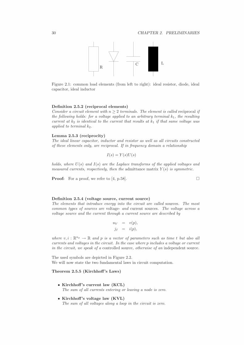
The symbol for a diode is found in Figure 2.1. In graphical representations of elec-trical networks, ideal resistors, capacitances and inductances are usually depicted asshown in Figure 2.1 and the symbols are labeled by ”R”, ”C” and ”L”, respectively.
30 CHAPTER 2. PRELIMINARIES
RC L
Figure 2.1: common load elements (from left to right): ideal resistor, diode, idealcapacitor, ideal inductor
Definition 2.5.2 (reciprocal elements)Consider a circuit element with n ≥ 2 terminals. The element is called reciprocal ifthe following holds: for a voltage applied to an arbitrary terminal k1, the resultingcurrent at k2 is identical to the current that results at k1 if that same voltage wasapplied to terminal k2.
Lemma 2.5.3 (reciprocity)The ideal linear capacitor, inductor and resistor as well as all circuits constructedof these elements only, are reciprocal. If in frequency domain a relationship
I(s) = Y (s)U(s)
holds, where U(s) and I(s) are the Laplace transforms of the applied voltages andmeasured currents, respectively, then the admittance matrix Y (s) is symmetric.
Proof: For a proof, we refer to [4, p.58].
Definition 2.5.4 (voltage source, current source)The elements that introduce energy into the circuit are called sources. The mostcommon types of sources are voltage- and current sources. The voltage across avoltage source and the current through a current source are described by
uV = v(p),
jI = i(p),
where v, i : Rnp → R and p is a vector of parameters such as time t but also all
currents and voltages in the circuit. In the case where p includes a voltage or currentin the circuit, we speak of a controlled source, otherwise of an independent source.
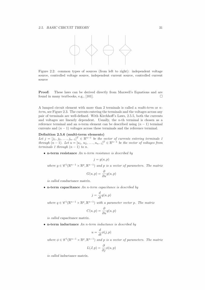
The used symbols are depicted in Figure 2.2.We will now state the two fundamental laws in circuit computation.
Theorem 2.5.5 (Kirchhoff’s Laws)
• Kirchhoff’s current law (KCL)The sum of all currents entering or leaving a node is zero.
• Kirchhoff’s voltage law (KVL)The sum of all voltages along a loop in the circuit is zero.
2.5. BASIC CIRCUIT THEORY 31
Figure 2.2: common types of sources (from left to right): independent voltagesource, controlled voltage source, independent current source, controlled currentsource
Proof: These laws can be derived directly from Maxwell’s Equations and arefound in many textbooks, e.g., [101].
A lumped circuit element with more than 2 terminals is called a multi-term or n-term, see Figure 2.3. The currents entering the terminals and the voltages across anypair of terminals are well-defined. With Kirchhoff’s Laws, 2.5.5, both the currentsand voltages are linearly dependent. Usually, the n-th terminal is chosen as areference terminal and an n-term element can be described using (n − 1) terminalcurrents and (n − 1) voltages across these terminals and the reference terminal.
Definition 2.5.6 (multi-term elements)Let j = [j1, j2, . . . , jn−1]
T ∈ Rn−1 be the vector of currents entering terminals 1
through (n − 1). Let u = [u1, u2, . . . , un−1]T ∈ Rn−1 be the vector of voltages from
terminals 1 through (n − 1) to n.
• n-term resistance An n-term resistance is described by
j = g(u, p)
where g ∈ C 1(Rn−1 × Rp, Rn−1) and p is a vector of parameters. The matrix
G(u, p) =∂
∂ug(u, p)
is called conductance matrix.
• n-term capacitance An n-term capacitance is described by
j =d
dtq(u, p)
where q ∈ C 1(Rn−1 × Rp, Rn−1) with a parameter vector p. The matrix
C(u, p) =∂
∂uq(u, p)
is called capacitance matrix.
• n-term inductance An n-term inductance is described by
u =d
dtφ(j, p)
where φ ∈ C 1(Rn−1 ×Rp, Rn−1) and p is a vector of parameters. The matrix
L(J, p) =∂
∂jφ(u, p)
is called inductance matrix.

32 CHAPTER 2. PRELIMINARIES
1 2 3
n (reference terminal)
Figure 2.3: n-term element
Definition 2.5.7 (RCL-circuits) A circuit that consists of independent sourcesand possibly nonlinear n-term resistances, n-term capacitances, and n-term capac-itances will be called RCL-circuit.
2.5.2 Modified Nodal Analysis
In the following, we will consider circuits with general nonlinear capacitances, resis-tances, inductances and voltage and current sources. We require that the controlledsources satisfy the restrictions given in Appendix B. We will briefly present twomodeling methods, namely the modified nodal analysis and the charge- and flux ori-ented modified nodal analysis. For a more detailed introduction to circuit modelingmethods we refer to [36].
Consider a circuit. Its topology is completely described by its reduced incidencematrix A and a reference node n⊤. The latter is also called ground or ground node.Let j be the vector of all branch currents, u the vector of all branch voltages and ethe vector of node potentials in the circuit. These terms are related by Kirchhoff’sCurrent Law and Kirchhoff’s Voltage Law, see Theorem 2.5.5. The statement ofthe KCL, that the sum of all currents that enter a node is equal to zero, can bewritten as
Aj = 0 (2.20)
for the whole circuit. The KVL translates into a relation between the branch volt-ages and the node potentials of the circuit
u = AT e. (2.21)
We now split the circuit into its capacitive, resistive and inductive subgraphs andinto those subgraphs that are defined by voltage and current sources. Here, abranch of the network graph that is occupied by a capacitance, resistance etc. isreferred to as capacitive, resistive, etc. branch. The subgraphs consisting of suchbranches only are accordingly called capacitive, resistive, etc. subgraphs. For thesesubgraphs, we define the vectors of branch currents j∗, branch voltages v∗ and therespective incidence matrices A∗, ∗ ∈ C, R, L, V, I for the capacitive, resistive andinductive part and the parts that are defined by voltage and current sources. The

2.5. BASIC CIRCUIT THEORY 33
respective terms for the whole circuit can be written as
j = [jTC , jT
R , jTL , jT
V , jTI ]T , (2.22a)
u = [uTC , uT
R, uTL , uT
V , uTI ]T , (2.22b)
A = [AC , AR, AL, AV , AI ]. (2.22c)
Thus, (2.20) together with (2.22a) and (2.22c) yields
Aj = ACjC + ARjR + ALjL + AV jV + AIiI = 0, (2.23)
and (2.21) together with (2.22b) and (2.22c) yields
u =
uC
uR
uL
uV
uI
=
ATCe
ATRe
ATLe
ATV e
ATI e
. (2.24)
To derive (2.23) and (2.24), we have only used information about the topology ofthe circuit. Now we describe the relations between the current through and thevoltage across a branch by the behavior of the element that defines this branch. Forthe resistive branches of the circuit, we get the relation
jR = g(uR, t). (2.25)
The relations for the capacitive and the inductive branches are
jC =d
dtq, q = qC(uC , t) (2.26)
and
uL =d
dtφ, φ = φL(jL, t), (2.27)
respectively. Here, q is the vector of charges of the capacitances and φ is the vectorof magnetic fluxes in the inductances of the circuit. Finally, the current and voltagesources are given by
jI = i(AT e,d
dtqC(AT
Ce, t), jL, jV , t) =: i(∗, t) (2.28)
and
uV = v(AT e,d
dtqC(AT
Ce, t), jL, jV , t) =: v(∗, t) (2.29)
(cf. [45]). Here, the ’*’ has been inserted for a shorter notation. Combination of thebranch relations (2.25), (2.26) and (2.27) and the description of the sources (2.28)and (2.29) with the information about the topology of the circuit, which is givenby (2.23) and (2.24), yields the following system
AC
d
dtq + ARg(AT
Re, t) + ALjL
+AV jV + AI i(∗, t) = 0, (2.30a)
ATLe − d
dtφ = 0, (2.30b)
ATV e − v(∗, t) = 0, (2.30c)
q − qC(ATCe, t) = 0, (2.30d)
φ − φL(jL, t) = 0. (2.30e)

34 CHAPTER 2. PRELIMINARIES
The procedure outlined above is the charge and flux oriented modified nodal analysis(MNA c/f). It yields a mixed system of differential and algebraic equations (DAE).The DAE (2.30) can be simplified if (2.30d) and (2.30e) are differentiated andinserted in (2.30a) and (2.30b). We define
C(uC , t) := ∂∂uC
qC(uC , t), qC,t(uC , t) := ∂∂t
qC(uC , t),
G(uR, t) := ∂∂uR
g(uR, t), g,t(uR, t) := ∂∂t
g(uR, t),
L(jL, t) := ∂∂jL
φL(jL, t), φL,t(jL, t) := ∂∂t
φL(jL, t).
The simplified system can then be written as
ACC(ATCe, t)
d
dt(AT
Ce) + ACqC,t(ATCe, t)
+ARG(ATRe, t)AT
Re + ARg,t(ATRe, t)
+ALjL + AV jV + AI i(∗, t) = 0, (2.31a)
ATLe − L(jL, t)
d
dtjL − φL,t(jL, t) = 0, (2.31b)
ATV e − v(∗, t) = 0, (2.31c)
This method is called modified nodal analysis (MNA). Like the MNA c/f method, theMNA leads to a DAE. Note that even though both (2.30) and (2.31) are analyticallyequivalent, there are situations in which (2.30) shows better numerical results than(2.31), also see [67, 105].
Definition 2.5.8 (passivity) A circuit is called passive if symm (C), symm(G)and symm (L) are all positive definite.
Passivity of a system is usually defined in an energy context. For electrical circuits,the simpler Definition 2.5.8 is found, e.g., in [4].
2.5.3 The matrices Y∗ and Z∗
We will subsequently need to compute some matrices that span the corange ofincidence matrices. It is advantageous to express them in terms of graph-relatedmatrices. In that way, numerical rank decisions can be avoided and roundoff errorsare reduced.In the following, we will call a matrix a basis of some subspace if its columns spanthat subspace.
2.5.3.1 The matrices YC and ZC
We define the matrix ZC to span a basis of corangeAC , that means, it is a matrixof maximal rank such that ZT
CAC = 0. Given a graph G of a circuit, we define thesubgraph GC(NC , BC) as the set of capacitive branches of G and all nodes of G.The incidence matrix of GC is AC and we can apply Lemma 2.4.24 to constructZC ∈ RN−1,FC−1, where FC is the number of components of GC .The matrix YC is defined in the following way. For every component of GC , wechoose one node. If the component contains the reference node, then choose thisnode. The set of nodes selected in this way will be denoted NC⊤
. The matrixYC ∈ RN−1,N−FC then consists all columns of the following form
[0 · · · 0 1 0 · · · 0]T
i,
where i is the index of a node in NC\NC⊤.

2.5. BASIC CIRCUIT THEORY 35
Lemma 2.5.9The matrix [YC , ZC ] is invertible.
Proof: We will prove the assertion for the case where GC consists of only onecomponent. If the component is connected to the ground, then the proof is trivialsince by Corollary 2.4.25, the number of columns of ZC vanishes and YC can bechosen INC
, where NC = |NC |.If the component does not contain the reference node, ZC = 1lNC
. We select onenode from NC . Without loss of generality let this be nNC
. Then, YC has the form
YC =
1. . .
10 · · · 0
and [YC , ZC ] is upper triangular with unit diagonal and hence nonsingular.The same proof is applicable, when GC consists of several components. In thatcase, the argument has to be applied to all components separately. By an appro-priately chosen permutation of columns, [YC , ZC ] can be reordered to become anupper triangular matrix with unit diagonal.
It is interesting to note that both matrices Y TC A and ZT
CA are again incidence ma-trices. Following the definition of YC , the matrix contains only unit vectors andin the product Y T
C A only those rows remain that belong to nodes in N\NC⊤. We
write Y TC AC = AC . The matrix AC can also be obtained as the incidence matrix
of the circuit graph G, where all nodes in NC⊤are identified with the ground node.
In a similar manner, it is possible to interpret ZTCA as the incidence matrix of the
graph G−C that arises from G by contracting the nodes that any capacitive branchis incident with into one node and subsequently deleting all capacitive branches.Such graph transformations are called contractions, also see [12, 18, 81].
2.5.3.2 The matrices YV −C, ZV −C and similar matrices
In the previous section, we have introduced ZTCA as the incidence matrix of G−C .
The matrix ZTCAR is the incidence matrix associated with the resistive branches
of G−C and ZTCAV is the incidence matrix associated with the branches occupied
by voltage sources. If we want to determine the corange of these matrices, we canproceed in a similar way to the construction of ZC . We consider ZV −C spanningcorange ZT
CAV . We define the graph GV −C as the subgraph of G−C that containsall branches occupied by voltage sources and all nodes of G−C . Let FV −C be thenumber of components of GV −C . The matrix ZV −C ∈ RFC−1,FV −C−1 can then bedefined using Lemma 2.4.24. Analogously to YC , we define YV −C ∈ RFC−1,FC−FV −C
as the incidence matrix of the subgraph of G−C , where all nodes not incident witha branch occupied by a voltage source are identified with the ground or grounded.
Remark 2.5.10 The analogously constructed matrices YR−C and ZR−C as well as
the matrix AR = Y TR−CAR, where resistive branches instead of branches occupied by
voltage sources are considered, will play an important role in the analysis of dynamiciteration methods for RCL circuits in Chapter 4.
It is possible to determine the product ZCV = ZCZV −C directly. By multiplyingA with ZT
C , all capacitive branches of G are contracted to yield G−C and then allbranches of G−C occupied by voltage sources are contracted. We call the resulting

36 CHAPTER 2. PRELIMINARIES
graph G−CV . This graph could also have been obtained by contracting all branchesof GCV , i.e., the graph consisting of branches occupied by capacitances or voltagesources and all nodes of G. Hence, we could have obtained ZCV in the first placeby applying Lemma 2.4.24 to GCV . This approach is especially advantageous forthe computation of ZCV by graph algorithms.Let GR−CV be the subgraph of G−CV that consist of all nodes of G−CV and allresistive branches. The matrices YR−CV and ZR−CV can be obtained from GR−CV
in the same way as YV −C and ZV −C have been obtained from GV −C . Additionally,the product ZCV R = ZCZV −CZR−CV can be obtained by applying Lemma 2.4.24to the subgraph GCV R which is constructed from G by contracting all edges withcapacitances, voltage sources and resistances. An overview on these special graphsis given in Table 2.1, while the graph-related matrices Y∗, Z∗ and A∗ are listed inTable 2.2.
2.5.3.3 The matrix ZV −C and related matrices
Following the notation introduced in [12], we define ZV −C such that range ZV −C =ker ZT
CAV . As it has been shown earlier, ZTCAV is the incidence matrix of the sub-
graph GV −C . In order to determine the kernel of this incidence matrix, we can useLemma 2.4.28 and choose ZV −C ∈ R
NV ,NCV to be the fundamental loop matrixof GV −C . Here, NV is the number of voltage sources in the circuit and NCV thenumber of fundamental loops in GV −C . We will later define other loop matriceswith respect to special sources in the GC , GR−C and GL−CR subgraphs.
2.5.4 Index and topology
In this subsection, we will show how to determine the index and the hidden alge-braic constraints of (2.30) and (2.31) with the help of the topology of the circuit.Consider a circuit where the controlled sources fulfill the restrictions stated in Ap-pendix B. The d-index of the DAEs (2.30) and (2.31) is linked to the topology ofthe circuit and is the same for both (2.30) and (2.31), cf. [45]. Thus, in this case, wemay speak of the d-index of the circuit. To state the relation between the topologyand the d-index of a circuit, we give the following definitions.
Definition 2.5.11 (CV-loop, LI-cutset)Consider the graph of a circuit.
1. An LI-cutset is a cutset consisting of inductances or both inductances andcurrent sources.
2. A CV-loop is a loop consisting of both capacitances and voltage sources.
Note, that there are no loops that only contain voltage sources and no cutsets thatonly consist of current sources, as these configurations may lead to inconsistencieswith Kirchhoff’s laws, [101].With the notion of CV-loops and LI-cutsets, it is possible to characterize the indexof a circuit and to state algebraic and hidden constraints in MNA equations.
Theorem 2.5.12 (d-index, algebraic and hidden constraints in MNA)Consider a DAE (2.31) that arises from MNA of a circuit. Under the assumptionthat all controlled sources fulfill the restrictions in Appendix B and that the matricesC(uC , t), G(uR, t) and L(jL, t) are positive definite for all uC , uR, jL and t, theconstraints within the MNA equations are given as follows.
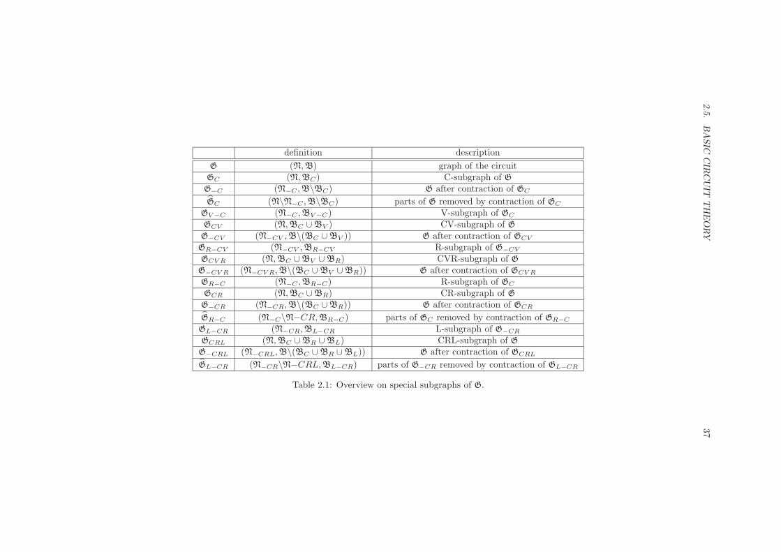
2.5
.B
ASIC
CIR
CU
ITT
HE
ORY
37
definition description
G (N, B) graph of the circuitGC (N, BC) C-subgraph of G
G−C (N−C , B\BC) G after contraction of GC
GC (N\N−C , B\BC) parts of G removed by contraction of GC
GV −C (N−C , BV −C) V-subgraph of GC
GCV (N, BC ∪ BV ) CV-subgraph of G
G−CV (N−CV , B\(BC ∪ BV )) G after contraction of GCV
GR−CV (N−CV , BR−CV R-subgraph of G−CV
GCV R (N, BC ∪ BV ∪ BR) CVR-subgraph of G
G−CV R (N−CV R, B\(BC ∪ BV ∪ BR)) G after contraction of GCV R
GR−C (N−C , BR−C) R-subgraph of GC
GCR (N, BC ∪ BR) CR-subgraph of G
G−CR (N−CR, B\(BC ∪ BR)) G after contraction of GCR
GR−C (N−C\N−CR, BR−C) parts of GC removed by contraction of GR−C
GL−CR (N−CR, BL−CR L-subgraph of G−CR
GCRL (N, BC ∪ BR ∪ BL) CRL-subgraph of G
G−CRL (N−CRL, B\(BC ∪ BR ∪ BL)) G after contraction of GCRL
GL−CR (N−CR\N−CRL, BL−CR) parts of G−CR removed by contraction of GL−CR
Table 2.1: Overview on special subgraphs of G.

38C
HA
PT
ER
2.
PR
ELIM
INA
RIE
S
definition description
A [AC , AR, AL, AV , AI ] split incidence matrix of G
ZC corange AC matrix performing contraction of GC in G
ZV −C corangeZTCAV matrix performing contraction of GV −C in G−C
ZCV = ZCZV −C , corange [AC , AV ] matrix performing contraction of GCV in G
ZR−CV corangeZTCV AR matrix performing contraction of GR−CV in G−CV
ZCV R = ZCZV −CZR−CV , corange [AC , AR, AV ] matrix performing contraction of GCV R in G
ZR−C corangeZTCAR matrix performing contraction of GR−C in G−C
ZCR = ZCZR−C , corange [AC , AR] matrix performing contraction of GCR in G
ZL−CR corangeZTCRAL matrix performing contraction of GL−CR in G−CR
ZCRL = ZCZR−CZL−CR, corange [AC , AR, AL] matrix performing contraction of GCRL in G
YC see above, [YC , ZC ] nonsing. selects certain nodes of GC
YR−C see above, [YR−C , ZR−C ] nonsing. selects certain nodes of GR−C
YL−CR as YC and YR−C , [YL−CR, ZL−CR] nonsing. selects certain nodes of GL−CR
AC Y TC AC incidence matrix of G where nodes in N\NC are grounded
AR Y TR−CZT
CAR incidence matrix of G−C where nodes in N−C\NR−C are grounded
AL Y TL−RCZT
R−CZTCAL incidence matrix of G−CR where nodes in N−CR\NL−CR are grounded
Table 2.2: Incidence matrices and selected graph-related matrices
2.5. BASIC CIRCUIT THEORY 39
1. If the circuit contains neither CV-loops nor LI-cutsets, then the d-index of theMNA equations is 1 and the DAE (2.31) does not contain hidden constraints.The algebraic constraints are
ZTC (ARg(AT
Re, t) + ALjL + AV jV + AIi(∗, t)) = 0,AT
V e − v(∗, t) = 0.(2.32)
2. If the circuit contains CV-loops but no LI-cutsets, then the d-index is 2. Thematrix ZV −C is non-zero and in addition to the algebraic constraints (2.32),the DAE (2.31) has the hidden constraints
ZTV −C(AT
V
d
dte − d
dtv(∗, t)) = 0. (2.33)
3. If the circuit contains LI-cutsets but no CV-loops, then the d-index is 2. Thematrix ZCV R is non-zero and in addition to the algebraic constraints (2.32),the DAE (2.31) has the hidden constraints
ZTCV R(AL
d
dtjL + AI
d
dti(∗, t)) = 0. (2.34)
4. If the circuit contains both CV-loops and LI-cutsets, then the d-index is 2. Thematrices ZV −C and ZCV R are non-zero and in addition to the algebraic con-straints (2.32), the DAE (2.31) has the hidden constraints (2.33) and (2.34).
Proof: For a proof, we refer to [45]. The special formulation of the constraints isfound in [12].

40 CHAPTER 2. PRELIMINARIES

Chapter 3
Dynamic Iteration Methods
We consider coupled systems of equations, more specifically ODEs and DAEs. Mostof today’s technical systems are composed of numerous different components, a factthat quite naturally divides the describing equations into coupled subsystems. Eachof these represents some aspects of the behaviour of the whole system and is thusbest treated separately. Usually, all subsystems have very different properties, bothanalytically and numerically. Instead of solving all systems at once with one solver,it has become a popular approach to solve coupled systems with coupled simu-lators. This approach is called co-simulation and has been studied widely in theliterature [9,39,120,132,137]. The main idea is to solve every subsystem on a smalltime window with an adequate solver. The solutions of the other subsystems haveto be approximated. This may be realized with the help of low order reduced mod-els for the other systems, see [121] or by extrapolating the solution of the last timewindow. Once every component has been dealt with, naturally the solution of onesubsystem differs from the approximation that all the others have been using intheir calculation. Hence, the whole process is iterated and every system now usesthe most recent solution of all other systems. This dynamic iteration process alsoknown as waveform relaxation is repeated until some sort of convergence has beenachieved, cf. [22, 80, 108]. Then, one proceeds to the next time-window and thewhole process is repeated.In the 1980s, this concept became popular in the simulation of partitioned electricalcircuits, cf. [51,64,99,110] and is still used today, sometimes in the form of MultirateMethods, [31, 61].
3.1 Dynamic Iteration for ODEs
The Dynamic Iteration Procedure as a means for solving systems of ordinary differ-ential equations has been widely investigated in literature, see, e.g., [16,22,80,104,108]. We will briefly define the structure of Dynamic Iteration Problems for ODEsand then state a theorem that explains the popularity of this approach.
Definition 3.1.1 (system of coupled ODEs)A set of N ODEs coupled as
y1 = f1(y1, y2, · · · , yN ),
... (3.1)
yN = fN (y1, y2, · · · , yN ),
41

42 CHAPTER 3. DYNAMIC ITERATION METHODS
where yi ∈ C 1(I, Rni), fi ∈ C L (Rn1 ×· · ·×RnN , Rni) will be called coupled systemof ODEs. Every equation of the form yi = fi(y1, y2, · · · , yN ), i = 1, . . . , N will becalled subsystem.
For convenience, we will only consider autonomous ODEs, i.e., fi does not explicitlydepend on t. This can always be assumed, since by adding the equation t = 1 toa non-autonomous ODE, t becomes a system variable and the ODE itself becomesautonomous.If the subsystems are not integrated together, then data from the other systemscome as a control input into each subsystem. This is usually realized with aniteration process, where for each subsystem previously computed iterates are usedas data for the solution of the other subsystems.
Definition 3.1.2 (Dynamic iteration method for ODEs, DIIVP)We will call a differential difference equation of the following form
y[k]1 = f1(Y
[k]1,1 , Y
[k]1,2 , · · · , Y
[k]1,N ),
... (3.2)
y[k]N = fN (Y
[k]N,1, Y
[k]N,2, · · · , Y
[k]N,N )
with Y[k]i,j =
lmax∑l=0
W[l]i,jy
[k−l]j , W
[l]i,j ∈ C 0(I, Rnj ,nj ) a dynamic iteration method (DIM)
of depth lmax for a system of coupled ODEs (3.1).Together with initial values y1,0 = y1(t0), . . . , yN,0 = yN (t0) and starting iterates
y[0]1 , . . . , y
[lmax−1]1 to y
[0]N , . . . , y
[lmax−1]N the DIM (3.2) is called dynamic iteration
initial value problem (DIIVP).
If y[l]i (t0) = yi,0, i = 1, . . . , N, l = 0, . . . , lmax − 1, then the starting iterates y
[l]i are
called consistent.
Theorem 3.1.3A consistent DIIVP (3.2) for a system of coupled ODEs (3.1) with the same initialvalues for (3.1) as for (3.2) and continuous starting iterates and with
lmax∑
l=0
W[l]i,j = I, i, j = 1, . . . , N
always converges to the solution of (3.1) for k → ∞.
Proof: A proof can be found in [40, 41].
This formulation also contains the special cases of the classic Picard-Iteration with
W[1]i,j = I, i, j = 1, . . . , N,
W[l]i,j = 0 else
or the block-Jacobi- and block-Gauss-Seidel-Iterations. We will put special emphasison the latter two methods in Section 3.3. The main statement of Theorem 3.1.3is that under some weak assumptions, a DIM (3.2) always converges to the correctsolution of a system of coupled ODEs (3.1). This effect has been used in variousapplications, e.g., [11, 34, 38, 79, 83, 133].
3.2. DYNAMIC ITERATION FOR DAES 43
3.2 Dynamic Iteration for DAEs
With increasing interest in differential-algebraic equations, the investigation of Dy-namic Iteration Methods for DAEs also became an issue. In this section, we willgeneralize the previous definitions to DAEs and state a convergence theorem forthese systems. Unfortunately, a result as strong as Theorem 3.1.3 does not exist forDAEs.
Definition 3.2.1 (system of coupled DAEs)A set of N DAEs that are coupled as
0 = F1(x1, x1, x2, · · · , xN ),
... (3.3)
0 = FN (xN , x1, x2, · · · , xN ),
where xi ∈ C 1(I, Rni), Fi ∈ C 1(Rni×Rn1×· · ·×R
nN , Rni) will be called coupled sys-tem of DAEs. Every equation of the form 0 = Fi(xi, x1, x2, · · · , xN ), i = 1, . . . , Nwill be called subsystem. The variables that appear as derivatives in a subsystemwill be denoted as variables belonging to a subsystem or local variables.
Remark 3.2.2 This is not the most general coupling between subsystems, as it isnot allowed for the derivatives of the variables of two subsystems to appear explic-itly in the same subsystem. Also, we do not consider over- or underdeterminedsubsystems.
As in the ODE case, we will only consider autonomous DAEs. We define a DIMand a DIIVP for DAEs in an analogous way to ODEs. Note that also in this caseonly the states and not the derivatives belonging to each subsystem are exchanged.
Definition 3.2.3 (DIM, DIIVP for DAEs)We will call a differential difference equation of the following form
0 = F1(x[k]1 , X
[k]1,1, X
[k]1,2, · · · , X
[k]1,N ),
... (3.4)
0 = FN (x[k]N , X
[k]N,1, X
[k]N,2, · · · , X
[k]N,N )
with X[k]i,j =
lmax∑l=0
W[l]i,jx
[k−l]j , W
[l]i,j ∈ C 0(I, Rnj ,nj ) a dynamic iteration method (DIM)
of depth lmax for a system of coupled DAEs (3.3).Conveniently, we define
x[k] =
x[k]1...
x[k]N
.
Given initial values x1,0 = x1(t0), . . . , xN,0 = xN (t0) and starting iterates x[0]1 , . . . , x
[lmax−1]1
to x[0]N , . . . , x
[lmax−1]N , the DIM (3.4) is called DIIVP for DAEs.
If x[l]i (t0) = xi,0, i = 1, . . . , N, l = 0, . . . , lmax − 1, then the starting iterates x
[l]i are
called consistent. If the DIIVP together with its starting iterates allows for iteratesx[k], k ≥ lmax to be computed, then the DIIVP is called consistent.

44 CHAPTER 3. DYNAMIC ITERATION METHODS
Remark 3.2.4 In the case when the coupled system (3.3) or any of its subsystemsis of d-index higher than 1, it may be possible that a set of initial values x1,0 =x1(t0), . . . , xN,0 = xN (t0) that is consistent with (3.3) is not consistent with theDAE (3.4) for a given step k.
We will subsequently only deal with consistent DIIVPs. Also, we will restrict ourconsiderations to DIMs of depth 1, as a variable substitution
x[k] = (x[k], x[k−1], . . . , x[k−lmax+1])
can be considered. Then, instead of mapping
(x[k], x[k−1], . . . , x[k−lmax+1]) → (x[k+1], x[k], . . . , x[k−lmax+2])
we just need to consider x[k] → x[k+1]. In that case, the DIIVP (3.4) can be writtenas
0 = F (x[k], x[k], x[k−1]). (3.5)
We will assume that the DAE (3.5) is of d-index 1 with respect to the variable x[k].Then, with Definition 2.3.4, its derivative array (2.11) is given as
F1(x[k], x[k], x[k], x[k−1], x[k−1]) =
[F (x[k], x[k], x[k−1])ddt
F (x[k], x[k], x[k−1])
]. (3.6)
From Definition 2.3.4, we also obtain that it is possible to transform F1 = 0 intothe underlying ODE of (3.5), given as the differential difference equation
x[k] = ϕ(x[k], x[k−1], x[k−1]). (3.7)
Remark 3.2.5 We restrict ourselves to the d-index 1 case as for higher indices, thederivative array (3.6) and also (3.7) may depend on higher derivatives of x[k−1]. Ifthis is the case then the iterates x[k] may depend on derivatives of increasing orderof x[0] and the method becomes numerically infeasible. In Chapter 4, we will stateseveral high index cases that still lead to reasonable DIMs.
We will now show, that under some conditions, the iteration defined by (3.7) con-verges to a limit x = limk→∞ x[k]. Due to the uniqueness of the limit, it solves
˙x = φ(x, x, ˙x)
or
0 = F (x, ˙x, x)
with F as in (3.5).
Theorem 3.2.6Given a sequence x[k] ∈ C 1(I, Rn), k = 1, . . . ,∞ defined by a differential differenceEquation (3.7) with ϕ ∈ C 2(Rn × R
n × Rn, Rn), a starting iterate x[0] ∈ C 1(I, Rn)
and an initial value x0 such that
x[k](t0) = x0, k = 1, . . . ,∞,
then the sequence
x[k], k = 0, . . . ,∞
converges uniformly to a limit function x if a constant L < 1 exists such that
‖ϕ,x[k−1](ξ[k], ξ[k−1], η[k−1])‖∞ ≤ L (3.8)
for arbitrary ξ[k], ξ[k−1], η[k−1] ∈ Rn.

3.2. DYNAMIC ITERATION FOR DAES 45
Proof: We transform (3.7) into an integral equation
x[k](t) = x[k](t0) +
∫ t
t0
ϕ(x[k](τ ), x[k−1](τ ), x[k−1](τ ))dτ. (3.9)
This integral operator maps the continuously differentiable function x[k−1] to acontinuously differentiable function x[k]. The space C 1(I, Rn) is mapped into it-self. Hence, in order to apply the BFPT 2.2.5, it suffices to show that (3.9) is acontraction on C 1(I, Rn). Let u[k−1] and v[k−1] be in C 1(I, Rn) and u[k−1](t0) =v[k−1](t0) = x0. Then, with (3.9) we have
u[k](t) − v[k](t)
=
t∫
t0
(ϕ(u[k](τ ), u[k−1](τ ), u[k−1](τ )) − ϕ(v[k](τ ), v[k−1](τ ), v[k−1](τ )))dτ.
We use the mean value theorem for vector valued functions, see [77], to obtain
ϕ(u[k](t), u[k−1](t), u[k−1](t)) − ϕ(v[k](t), v[k−1](t), v[k−1](t))
=
∫ 1
0
ϕ,x[k](ξ[k](t, h), ξ[k−1](t, h), η[k−1](t, h))dh · (u[k] − v[k])
+
∫ 1
0
ϕ,x[k−1](ξ[k](t, h), ξ[k−1](t, h), η[k−1](t, h))dh · (u[k−1] − v[k−1])
+
∫ 1
0
ϕ,x[k−1](ξ[k](t, h), ξ[k−1](t, h), η[k−1](t, h))dh · (u[k−1] − v[k−1])
with
ξ[k](t, h) = v[k](t) + h(u[k](t) − v[k](t)),
ξ[k−1](t, h) = v[k−1](t) + h(u[k−1](t) − v[k−1](t)),
η[k−1](t, h) = v[k−1](t) + h(u[k−1](t) − v[k−1](t)).
We define the matrices
Φx[k](·, ·, ·) =
∫ 1
0
ϕ,x[k](·, ·, ·)dh, (3.10a)
Φx[k−1](·, ·, ·) =
∫ 1
0
ϕ,x[k−1](·, ·, ·)dh, (3.10b)
Φx[k−1](·, ·, ·) =
∫ 1
0
ϕ,x[k−1](·, ·, ·)dh (3.10c)
and we set
Lx[k] = maxξ[k],ξ[k−1],η[k−1]∈Rn
‖Φx[k](ξ[k], ξ[k−1], η[k−1])‖∞,
Lx[k−1] = maxξ[k],ξ[k−1],η[k−1]∈Rn
‖Φx[k−1](ξ[k], ξ[k−1], η[k−1])‖∞,
Lx[k−1] = maxξ[k],ξ[k−1],η[k−1]∈Rn
‖Φx[k−1](ξ[k], ξ[k−1], η[k−1])‖∞,
Lx[k−1],t = maxξ[k],ξ[k−1],η[k−1]∈Rn
‖ d
dtΦx[k−1](ξ[k], ξ[k−1], η[k−1])‖∞.
As ϕ is in C 2 and I is a bounded interval all these values are well defined and finite.For a shorter notation, we omit the arguments in the Φ terms and with the above
46 CHAPTER 3. DYNAMIC ITERATION METHODS
definitions we have
u[k](t) − v[k](t) =
t∫
t0
Φx[k] · (u[k] − v[k])dτ (3.11)
+
t∫
t0
Φx[k−1] · (u[k−1] − v[k−1])dτ (3.12)
+
t∫
t0
Φx[k−1] · (u[k−1] − v[k−1])dτ.
We want to investigate whether the integral operator defined by (3.9) is a contrac-tion in a suitably chosen ‖ · ‖∞,α norm.
‖u[k] − v[k]‖∞,α = ‖e−αt(u[k](t) − v[k](t))‖∞
=
∥∥∥∥∥∥e−αt
t∫
t0
Φx[k](u[k] − v[k])dτ
+
t∫
t0
Φx[k−1](u[k−1] − v[k−1])dτ
+
t∫
t0
Φx[k−1](u[k−1] − v[k−1])dτ
∥∥∥∥∥∥∞
.
Hence,
‖u[k] − v[k]‖∞,α ≤
∥∥∥∥∥∥e−αt
t∫
t0
Φx[k](u[k] − v[k])dτ
∥∥∥∥∥∥∞
+
∥∥∥∥∥∥e−αt
t∫
t0
Φx[k−1](u[k−1] − v[k−1])dτ
∥∥∥∥∥∥∞
(3.13)
+
∥∥∥∥∥∥e−αt
t∫
t0
Φx[k−1](u[k−1] − v[k−1])dτ
∥∥∥∥∥∥∞
.
We then determine bounds for each summand:∥∥∥∥∥∥e−αt
t∫
t0
Φx[k](u[k](τ ) − v[k](τ ))dτ
∥∥∥∥∥∥∞
=
∥∥∥∥∥∥∥e−αt
t∫
t0
Φx[k]eατ e−ατ (u[k](τ ) − v[k](τ ))︸ ︷︷ ︸≤‖u[k]−v[k]‖∞,α
dτ
∥∥∥∥∥∥∥∞
≤
∥∥∥∥∥∥e−αt
t∫
t0
Φx[k]eατdτ
∥∥∥∥∥∥∞
‖u[k] − v[k]‖∞,α
≤ 1
α(1 − e−α(t−t0))Lx[k]‖u[k] − v[k]‖∞,α.
3.2. DYNAMIC ITERATION FOR DAES 47
As t ≥ t0 we have
∥∥∥∥∥∥e−αt
t∫
t0
Φx[k](u[k] − v[k])dτ
∥∥∥∥∥∥∞
≤ 1
αLx[k]‖u[k] − v[k]‖∞,α. (3.14)
In an analogous way, we obtain
∥∥∥∥∥∥e−αt
t∫
t0
Φx[k−1](u[k−1] − v[k−1])dτ
∥∥∥∥∥∥∞
≤ 1
αLx[k−1]‖u[k−1] − v[k−1]‖∞,α. (3.15)
For the last summand, the bound is different. We integrate by parts and obtain
∥∥∥∥∥∥e−αt
t∫
t0
Φx[k−1](u[k−1](τ ) − v[k−1](τ ))dτ
∥∥∥∥∥∥∞
(3.16)
=
∥∥∥∥∥∥e−αtΦx[k−1](u[k−1](t) − v[k−1](t)) − e−αt
t∫
t0
d
dτΦx[k−1](u[k−1](τ ) − v[k−1](τ ))dτ
∥∥∥∥∥∥∞
.
This expression can be bounded as
∥∥∥∥∥∥e−αt
t∫
t0
Φx[k−1](u[k−1](τ ) − v[k−1](τ ))dτ
∥∥∥∥∥∥∞
≤ Lx[k−1]‖u[k−1] − v[k−1]‖∞,α +1
αLx[k−1],t‖u[k−1] − v[k−1]‖∞,α. (3.17)
So, from (3.13) together with (3.14), (3.15) and (3.17) we have
‖u[k] − v[k]‖∞,α ≤ 1
αLx[k]‖u[k] − v[k]‖∞,α (3.18)
+(1
αLx[k−1] +
1
αLx[k−1],t + Lx[k−1])‖u[k−1] − v[k−1]‖∞,α,
‖u[k] − v[k]‖∞,α ≤1αLx[k−1] + 1
αLx[k−1],t + Lx[k−1]
1 − 1αLx[k]
︸ ︷︷ ︸!=L
‖u[k−1] − v[k−1]‖∞,α.
For α sufficiently large, L is arbitrarily close to Lx[k−1] . More precisely, if Lx[k−1] < 1
and α >L
x[k]+Lx[k−1]+L
x[k−1],t
1−Lx[k−1]
then L < 1. Application of the BFPT 2.2.5 shows
that the integral operator (3.9) is a contraction. With the definition of Lx[k−1] andΦx[k−1] , it follows that Lx[k−1] ≤ L. Hence, if L < 1, then Lx[k−1] < 1 which con-cludes the proof.
The convergence of the dynamic iteration method can be related to the quasi-nilpotency of dynamic iteration operators, cf. [109]. This allows for a weaker con-vergence criterion.
Corollary 3.2.7Under the otherwise identical assumptions as in Theorem 3.2.6, the requirement(3.8) can be weakened to
‖(Φx[k−1])ν‖∞ < 1,
48 CHAPTER 3. DYNAMIC ITERATION METHODS
with Φx[k−1] as in (3.10), for some integer ν ≥ 1. Going even further, for the limitcase ν → ∞, this translates to ρ(Φx[k−1]) < 1, where
ρ(Φx[k−1]) = max(ρ(Φx[k−1](ξ[k], ξ[k−1], η[k−1])), ξ[k], ξ[k−1], η[k−1] ∈ Rn)
and ρ(·) denotes the spectral radius of a matrix.
Proof: We state a proof for the case ν = 2, while the proof for ν > 2 is straightfor-ward. The equivalence to the spectral radius can be found in [78, Theorem 5.7.10].We will state a bound similar to (3.18) but for two consecutive steps. Using thesame notation as in the proof of Theorem 3.2.6, we have from (3.13) that
‖u[k] − v[k]‖∞,α ≤
∥∥∥∥∥∥e−αt
t∫
t0
Φx[k](u[k] − v[k])dτ
∥∥∥∥∥∥∞
+
∥∥∥∥∥∥e−αt
t∫
t0
Φx[k−1](u[k−1] − v[k−1])dτ
∥∥∥∥∥∥∞
+
∥∥∥∥∥∥e−αt
t∫
t0
Φx[k−1](u[k−1] − v[k−1])dτ
∥∥∥∥∥∥∞
and with (3.14), (3.15) and (3.16) we obtain
‖u[k] − v[k]‖∞,α ≤ 1
αLx[k]‖u[k] − v[k]‖∞,α (3.19)
+1
α
(Lx[k−1] + Lx[k−1],t
)‖u[k−1] − v[k−1]‖∞,α
+∥∥∥e−αtΦx[k−1](u[k−1] − v[k−1])
∥∥∥∞
.
We investigate the last summand more closely. We replace (u[k−1] − v[k−1]) withthe help of (3.11) and use (3.14), (3.15) and (3.16) again to obtain
∥∥∥e−αtΦx[k−1](u[k−1] − v[k−1])∥∥∥∞
(3.20)
≤ Lx[k−1]
αLx[k]‖u[k−1] − v[k−1]‖∞,α
+Lx[k−1]
α
(Lx[k−1] + Lx[k−1],t
)‖u[k−2] − v[k−2]‖∞,α
+∥∥∥e−αtΦ2
x[k−1](u[k−2] − v[k−2])
∥∥∥∞
.
Theoretically, we have a similar bound as in (3.19) and we could proceed analogouslyfor the last summand. However, we only show the case ν = 2 and use the bound
∥∥∥e−αtΦ2x[k−1](u
[k−2] − v[k−2])∥∥∥∞
≤ ‖Φ2x[k−1]‖∞‖(u[k−2] − v[k−2])‖∞,α.
Together with (3.19) and (3.20), we obtain
‖u[k] − v[k]‖∞,α ≤ 1
αLx[k]‖u[k] − v[k]‖∞,α
+1
α
(Lx[k−1] + Lx[k−1],t + Lx[k−1]Lx[k]
)‖u[k−1] − v[k−1]‖∞,α
+Lx[k−1]
α
(Lx[k−1] + Lx[k−1],t
)‖u[k−2] − v[k−2]‖∞,α
+‖Φ2x[k−1]‖∞‖(u[k−2] − v[k−2])‖∞,α.
3.2. DYNAMIC ITERATION FOR DAES 49
We replace the occurrences of ‖u[k]−v[k]‖∞,α and ‖u[k−1] −v[k−1]‖∞,α on the righthand side with the help of (3.18) and obtain
‖u[k] − v[k]‖∞,α ≤ L‖u[k−2] − v[k−2]‖∞,α
where
L =1
1 − Lx[k]
α
(Lx[k−1]
α
(Lx[k−1] + Lx[k−1],t
)+
L
α
(Lx[k−1] + Lx[k−1],t + Lx[k−1]Lx[k]
)
+L2
αLx[k] + ‖Φ2
x[k−1]‖∞)
.
We see that for α → ∞, L comes arbitrarily close to ‖Φ2x[k−1]‖∞ and with analogous
reasoning as in the proof of Theorem 3.2.6, we obtain the assertion.
Corollary 3.2.8With identical assumptions as in Theorem 3.2.6, but ϕ depending explicitly on t,i.e.,
x[k] = ϕ(t, x[k], x[k−1], x[k−1]),
the convergence criterion becomes ρ(Φx[k−1]) < 1 with
ρ(Φx[k−1]) = max(ρ(Φx[k−1](t, ξ[k], ξ[k−1], η[k−1])), t ∈ I, ξ[k], ξ[k−1], η[k−1] ∈ Rn)
where Φx[k−1] is now depending on t:
Φx[k−1](t, ξ[k], ξ[k−1], η[k−1]) =
∫ 1
0
ϕ,x[k](t, ξ[k], ξ[k−1], η[k−1]))dh.
Proof: The proof is analogous to the proofs of Theorem 3.2.6 and Corollary 3.2.7together.
Remark 3.2.9 The assumption that ρ(Φx[k−1]) < 1 is still rather strong as themaximum spectral radius over all possible arguments ξ[k], ξ[k−1] and η[k−1] has to bedetermined. For specific initial values and intervals I, a more localized result maybe obtained. However, in this work, we will mainly deal with linear systems, whereΦx[k−1] is constant and independent of ξ[k], ξ[k−1] and η[k−1].
Definition 3.2.10A DIM as in Theorem 3.2.6 with ρ(Φx[k−1]) = 0 will be called quasi-instantaneouslyconvergent.
With this definition, all DIMs for coupled systems of ODEs (3.2) have quasi-instantaneous convergence. For systems of coupled algebraic equations or DAEs(3.4) this cannot be expected in general. However, under certain assumptions, somespecially structured systems can be transformed to exhibit quasi-instantaneous con-vergence.
Remark 3.2.11 Quasi-instantaneous convergence can still be rather slow, depend-ing on the constants Lx[k] , Lx[k−1] and Lx[k],t. However, for arbitrary consistent
x[0], on a sufficiently small interval [t0, t1], the first iterate x[1] is arbitrarily closeto the correct solution. In Chapter 5, we will investigate this effect in more detail.

50 CHAPTER 3. DYNAMIC ITERATION METHODS
Example 3.2.12 Consider the following DAE
y =
[0 −11 0
]y, (3.21a)
0 = y + (I − A)z (3.21b)
with
y =
[y1
y2
], z =
[z1
z2
], A =
[a11 a12
a21 a22
].
We state the following dynamic iteration method for the solution of (3.21).
y[k]1 = −y
[k−1]2 , (3.22a)
0 = y[k]1 + z
[k]1 − a11z
[k−1]1 − a12z
[k−1]2 , (3.22b)
y[k]2 = y
[k−1]1 , (3.23a)
0 = y[k]2 + z
[k]2 − a21z
[k−1]1 − a22z
[k−1]2 . (3.23b)
Obviously, y[k]1 and y
[k]2 are defined by Equations (3.22a) and (3.23a) alone. This is
a system of coupled ODEs. Hence, with Theorem 3.1.3, convergence is guaranteedand quasi-instantaneous for arbitrary initial values y1,0 and y2,0 and continuousstarting iterates. For the whole system (3.22) with (3.23), this does not necessarilyhold. We differentiate Equations (3.22b) and (3.23b) and reorder the whole systemas
[I 0I I
]
y1
y2
z1
z2
[k]
=
0 −11 0
00
y1
y2
z1
z2
[k−1]
+
[0
A
]
y1
y2
z1
z2
[k−1]
. (3.24)
By multiplying
[I 0I I
]−1
from the left, we obtain a recurrence
y1
y2
z1
z2
[k]
=
0 −11 00 1 0−1 0 0
y1
y2
z1
z2
[k]
+
[0
A
]
y1
y2
z1
z2
[k−1]
, (3.25)
which is of the form (3.7). Corollary 3.2.7 now states that the rate of convergenceof the recurrence (3.25) is determined by the spectral radius ρ(A). We already
mentioned, that the recurrence for
[y1
y2
][k]
converges. If A in (3.25) vanishes,
then
[z1
z2
][k]
= −[
y1
y2
][k]
and convergence for the whole vector is determined by
the convergence of
[y1
y2
][k]
. Otherwise, convergence of
[z1
z2
][k]
depends on the
behaviour of the homogeneous difference equation
[z1
z2
][k]
= A
[z1
z2
][k−1]
.
3.2. DYNAMIC ITERATION FOR DAES 51
By Lemma 2.1.22, this is only the case if ρ(A) < 1.Hence, for
A =
[2 00 0
],
we have ρ(A) = 2 and the method diverges while for
A =
[0 20 0
],
we have ρ(A) = 0 and the method is quasi-instantaneously convergent, even though‖A‖∞ = 2 in both cases.
For the case of LTI DAEs, we consider a generalization of Theorem 3.2.6. Weconsider functions x[k], where x[k] ∈ C ℓ(I, Rn), k ∈ N0 with sufficiently large ℓ andx[k](t0) = 0. Without loss of generality, we assume that t0 = 0 in I = [t0, t0 + T ].Then, with I compact and x[k] bounded, we have x[k] ∈ L2(I, R
n), k ∈ N0. Let
x[k](t) =
x[k](t) for t ∈ I
0 else,(3.26)
Hence, x[k] ∈ L2(R+, Rn). Let X(s)[k] = L (x[k]) be the Laplace transform, 2.2.11of x[k]. Then the following theorem holds.
Theorem 3.2.13Consider a linear time-invariant mapping
g : x[k−1] 7→ x[k].
Via x[k] as in (3.26) and X [k] = L (x[k]), this mapping also defines a recurrence infrequency domain by
X [k](s) = G(s)X [k−1](s), (3.27)
where G : C → Cn,n is a rational function in s. The recurrence x[k−1] → x[k] that
is defined in frequency domain by equation (3.27) converges to x[∞] = 0 on I if Gis proper and the spectral radius ρ(G∞) < 1, where G∞ = lims→∞ G(s).
Proof: We will not prove the statement in frequency domain, but rather in timedomain. As G is assumed to be proper, we may set
G(s) = G∞ + Gsp(s),
where Gsp is strictly proper. With Theorem 2.2.12, we have
X [k](s) = G∞X [k−1](s) + Gsp(s)X[k−1](s). (3.28)
Using Theorem 2.2.12 again, Equation (3.27) is equivalent to
x[k](t) = G∞x[k−1](t) +
t∫
0
gsp(τ )x[k−1](t − τ )dτ, (3.29)
where L (gsp) = Gsp. As G has been assumed to be rational, then so is Gsp and wecan perform a decomposition into partial fractions as
Gsp(s) =
np∑
i
pi∑
j=1
Aij
1
(s − λi)j.

52 CHAPTER 3. DYNAMIC ITERATION METHODS
Here, λi ∈ C are the poles of Gsp(s) and pi are the multiplicities of these poles.Furthermore, Aij ∈ C
n,n, and np is the number of pairwise distinct poles. With thehelp of a table of common Laplace transforms, e.g., in [20], we find
gsp(t) =
np∑
i
pi∑
j=1
Aij
ti−1
(i − 1)!eλit.
Hence, gsp ∈ C ∞(R+, Cn,n) but also gsp ∈ C ∞(I, Cn,n) and ‖gsp‖∞ < ∞, if themaximum is considered only on I.We consider (3.29) and multiply with e−αt.
e−αtx[k](t) = G∞e−αtx[k−1](t) + e−αt
t∫
0
gsp(τ )x[k−1](t − τ )dτ
= G∞e−αtx[k−1](t) +
t∫
0
gsp(τ )e−ατe−α(t−τ)x[k−1](t − τ )dτ.
We take ‖ ·‖∞ norms and after replacing with the ‖ ·‖∞,α norm, where appropriate,we obtain
‖e−αtx[k](t)‖∞ =
∥∥∥∥∥∥G∞e−αtx[k−1](t) +
t∫
0
gsp(τ )e−ατe−α(t−τ)x[k−1](t − τ )dτ
∥∥∥∥∥∥∞
,
‖x[k]‖∞,α ≤ ‖G∞‖∞‖x[k−1]‖∞,α +
∥∥∥∥∥∥
t∫
0
gsp(τ )e−ατdτ
∥∥∥∥∥∥∞
‖x[k−1]‖∞,α. (3.30)
With ‖gsp(s)‖∞ < ∞ the integral expression can be bounded as
∥∥∥∥∥∥
t∫
0
gsp(τ )e−ατdτ
∥∥∥∥∥∥∞
≤ ‖gsp‖∞
∥∥∥∥∥∥
t∫
0
e−ατdτ
∥∥∥∥∥∥∞
≤ ‖gsp‖∞
∥∥∥∥∥∥1
α(1 − e−αt)︸ ︷︷ ︸
<1
∥∥∥∥∥∥∞
≤ ‖gsp‖∞α
.
Hence, we have
‖x[k]‖∞,α ≤(‖G∞‖∞ +
‖gsp‖∞α
)‖x[k−1]‖∞,α
and for sufficiently large α, the expression(‖G∞‖∞ +
‖gsp‖∞
α
)comes arbitrarily
close to ‖G∞‖∞. The Banach Fixed Point Theorem 2.2.5 yields ‖G∞‖∞ < 1 as acriterion for convergence. We can employ the same argument as in Corollary 3.2.7to show that instead of ‖G∞‖∞ < 1, the requirement ρ(G∞) < 1 suffices.
Remark 3.2.14 The term of quasi-instantaneous convergence also applies in theLTI case if ‖G∞‖∞ = 0, i.e., G(s) is strictly proper.
3.2. DYNAMIC ITERATION FOR DAES 53
Example 3.2.15 Consider the DIM (3.22) with (3.23) from Example 3.2.12 again.Let
Y0 =
[y1,0
y2,0
], Y [k] =
[Y1
Y2
][k]
=
[L (y
[k]1 )
L (y[k]2 )
], Z [k] =
[Z1
Z2
][k]
=
[L (z
[k]1 )
L (z[k]2 )
].
For simplicity, we assume Y0 = 0. We perform a Laplace transformation of (3.22)and (3.23) to obtain
sY[k]1 = −Y
[k−1]2 + y1,0, (3.31a)
0 = Y[k]1 + Z
[k]1 − a11Z
[k−1]1 − a12Z
[k−1]2 , (3.31b)
sY[k]2 = Y
[k−1]1 + y2,0, (3.32a)
0 = Y[k]2 + Z
[k]2 − a21Z
[k−1]1 − a22Z
[k−1]2 . (3.32b)
We can write this system as
Y [k] =1
s
[0 −11 0
]Y [k−1], (3.33a)
Z [k] =1
s
[0 1−1 0
]Y [k−1] + AZ [k−1]. (3.33b)
We immediately see that Equation (3.33a) alone is quasi-instantaneously convergentby Theorem 3.2.13 as the matrix function
1
s
[0 −11 0
]
is strictly proper. Let
X [k] =
[YZ
][k]
.
Then (3.33) can be written as
X [k] =
1s
[0 −11 0
]0
1s
[0 1−1 0
]A
︸ ︷︷ ︸G(s)
X [k−1]. (3.34)
The matrix function G(s) can be split into a strictly proper part Gsp(s) and a con-stant part G∞ as
G(s) =
1s
[0 −11 0
]0
1s
[0 1−1 0
]0
︸ ︷︷ ︸Gsp(s)
+
[0 00 A
]
︸ ︷︷ ︸G∞
.
Theorem 3.2.13 states that convergence of (3.34) is equivalent to ρ(G∞) = ρ(A) < 1and that the method is quasi-instantaneously convergent if ρ(G∞) = ρ(A) = 0 whichis the exact same result as in Example 3.2.12.

54 CHAPTER 3. DYNAMIC ITERATION METHODS
3.3 Gauss-Seidel and Jacobi methods
The dynamic iteration methods (3.2) and (3.4) are rather general in structure. Inpractice however, usually some specially structured schemes are used.
Definition 3.3.1A DIM (3.2) or (3.4) of depth 1 with
W[0]i,j =
I, i = j0, i 6= j
, W[1]i,j =
I, i 6= j0, i = j
is called Jacobi-type DIM.A DIM (3.2) or (3.4) of depth 1 with
W[0]i,j =
I, i ≤ j0, i > j
, W[1]i,j =
I, i > j0, i ≤ j
is called Gauss-Seidel-type DIM.
The terms Jacobi- and Gauss-Seidel-method originate in the iterative solution oflinear systems, see, e.g., [131]. The respective dynamic iteration methods are gener-alizations to ODEs or DAEs. In the case of the Jacobi-DIM, only the local variablesare updated in every iteration step while in every subsystem the solutions for allnon-local variables are taken from the previous iterate. This method offers greatpotential for parallelization. If all subsystems of (3.2) or (3.4) are treated sequen-tially instead of simultaneously, then once the solution of a subsystem has beencomputed, it can be used for all subsequent subsystems. In that way, more recentdata can be used than for the Jacobi-method. The method described is the Gauss-Seidel-DIM.
System 1
System 1
System 2
System 2x
[n−1]1 x
[n−1]1
x[n−1]2 x
[n−1]2
x[n]1 x
[n]1
x[n]2 x
[n]2
Figure 3.1: Schematic representation of the Jacobi (left) and Gauss-Seidel-DIM(right) for two systems
We will mainly deal with DIIVPs for semi-explicit DAEs. For systems structuredin this way, it becomes relatively easy to characterize convergence of DIMs. Also,for simplicity, we will only consider two subsystems
y1 = f1(y1, z1, y2, z2),0 = g1(y1, z1, y2, z2),
y2 = f2(y1, z1, y2, z2),0 = g2(y1, z1, y2, z2).
(3.35)
The Jacobi-method for two semi-explicit DAEs takes the form
y[k]1 = f1(y
[k]1 , z
[k]1 , y
[k−1]2 , z
[k−1]2 ),
0 = g1(y[k]1 , z
[k]1 , y
[k−1]2 , z
[k−1]2 ),
y[k]2 = f2(y
[k−1]1 , z
[k−1]1 , y
[k]2 , z
[k]2 ),
0 = g2(y[k−1]1 , z
[k−1]1 , y
[k]2 , z
[k]2 ).
(3.36)

3.3. GAUSS-SEIDEL AND JACOBI METHODS 55
Every subsystem is a DAE of d-index 1 if the Jacobian gi,zi, i = 1, 2 is nonsingular.
We regroup the variables and the equations. For simplicity, we retain the names forthe functions with differently ordered arguments
y[k]1 = f1(y
[k]1 , y
[k−1]2 , z
[k]1 , z
[k−1]2 ),
y[k]2 = f2(y
[k−1]1 , y
[k]2 , z
[k−1]1 , z
[k]2 ),
0 = g1(y[k]1 , y
[k−1]2 , z
[k]1 , z
[k−1]2 ),
0 = g2(y[k−1]1 , y
[k]2 , z
[k−1]1 , z
[k]2 ).
(3.37)
For the Gauss-Seidel method, the subsystems have the form
y[k]1 = f1(y
[k]1 , z
[k]1 , y
[k−1]2 , z
[k−1]2 ),
0 = g1(y[k]1 , z
[k]1 , y
[k−1]2 , z
[k−1]2 ),
y[k]2 = f2(y
[k]1 , z
[k]1 , y
[k]2 , z
[k]2 ),
0 = g2(y[k]1 , z
[k]1 , y
[k]2 , z
[k]2 ).
(3.38)
Also in this case, the index of a subsystem is determined by the nonsingularity ofgi,zi
, i = 1, 2. The reordered and regrouped system has the form
y[k]1 = f1(y
[k]1 , y
[k−1]2 , z
[k]1 , z
[k−1]2 ),
y[k]2 = f2(y
[k]1 , y
[k]2 , z
[k]1 , z
[k]2 ),
0 = g1(y[k]1 , y
[k−1]2 , z
[k]1 , z
[k−1]2 ),
0 = g2(y[k]1 , y
[k]2 , z
[k]1 , z
[k]2 ).
(3.39)
It can be seen, that both the Jacobi- and Gauss-Seidel-DIM applied to semi-explicitDAEs generate a semi-explicit DAE. We will subsequently treat the dynamic iter-ation DAEs (3.37) and (3.39) as their structure is closest to that of a semi-explicitDAE.
Definition 3.3.2Given a semi-explicit DAE arising from a DIM of the form
y[k] = f(y[k], y[k−1], z[k], z[k−1]),
0 = g(y[k], y[k−1], z[k], z[k−1])
with
f =
[f1
f2
], g =
[g1
g2
], y[k] =
[y[k]1
y[k]2
], z[k] =
[z[k]1
z[k]2
], (3.40)
we define the Jacobians
G[0]y =
∂g
∂y[k], G[1]
y =∂g
dy[k−1],
G[0]z =
∂g
∂z[k], G[1]
z =∂g
dz[k−1].
Lemma 3.3.3 (Index of Jacobi- and Gauss-Seidel DIMs for semi-explicit DAEs)
The systems (3.37) and (3.39) are DAEs for
[y[k]
z[k]
]of d-index 1 if and only
if the respective subsystems are DAEs of d-index 1.
Proof: With Lemma 2.3.7, we have that each subsystem is a DAE of d-index 1 ifand only if gi,zi
, i = 1, 2 is nonsingular.
For the Jacobi-DIM, G[0]z has the form
G[0]z =
[g1,z1
00 g2,z2
]

56 CHAPTER 3. DYNAMIC ITERATION METHODS
and in the case of a Gauss-Seidel method
G[0]z =
[g1,z1
0g2,z1
g2,z2
].
In both cases, G[0]z is block lower triangular. This matrix is nonsingular if and only
if g1,z1and g2,z2
are both nonsingular, i.e., if and only if both subsystems are ofd-index 1. Using Lemma 2.3.7 on (3.37) or (3.39), we obtain the assertion.
Remark 3.3.4 For N > 2 subsystems, the matrix G[0]z has the form
G[0]z =
g1,z1
. . .
gN,zN
for the Jacobi-DIM and
G[0]z =
g1,z1
.... . .
gN,z1· · · gN,zN
in the case of the Gauss-Seidel DIM. It can easily be seen from the structure of G[0]z
that the claim of Lemma 3.3.3 carries over to more than two subsystems.
Theorem 3.3.5A Jacobi- or Gauss-Seidel-DIM ((3.36) or (3.38)) for a coupled system of two semi-explicit DAEs (3.35) of d-index 1 converges if
max(ρ(g−12,z2
g2,z1g−11,z1
g1,z2)) < 1,
where the maximum is taken over all arguments (η1, ζ1, η2, ζ2) ∈ Rn1d × Rn1a ×Rn2d × Rn2a .
Proof: We will use the reordered equations (3.37) and (3.39). Both have a formas in Definition 3.3.2 and with Lemma 3.3.3, the DAE system is of d-index 1. Wecompute the uODE of the respective system and obtain an implicit ODE of theform[
I 0
−G[0]y −G
[0]z
] [y[k]
z[k]
]=
[f(y[k], y[k−1], z[k], z[k−1])
0
]+
[0 0
G[1]y G
[1]z
] [y[k−1]
z[k−1]
]
or
[y[k]
z[k]
]=
[I 0
−G[0]y −G
[0]z
]−1 [f(y[k], y[k−1], z[k], z[k−1])
0
]
+
[I 0
−G[0]y −G
[0]z
]−1 [0 0
G[1]y G
[1]z
] [y[k−1]
z[k−1]
]. (3.41)
Equation (3.41) is a differential-difference equation as in (3.7) and with Theorem3.2.6, we have convergence of the DIM if
∥∥∥∥∥
[I 0
−G[0]y −G
[0]z
]−1 [0 0
G[1]y G
[1]z
]∥∥∥∥∥∞=
∥∥∥∥∥
[0 0
−(G
[0]z
)−1
G[1]y −
(G
[0]z
)−1
G[1]z
]∥∥∥∥∥∞
< 1.
3.3. GAUSS-SEIDEL AND JACOBI METHODS 57
With Corollary 3.2.7 this condition translates to
ρ
((G[0]
z
)−1
G[1]z
)< 1.
For the Gauss-Seidel-DIM, the matrix(G
[0]z
)−1
G[1]z has the form
(G[0]
z
)−1
G[1]z =
[g1,z1
0g2,z1
g2,z2
]−1 [0 g1,z2
0 0
]
=
[0 g−1
1,z1g1,z2
0 −g−12,z2
g2,z1g−11,z1
g1,z2
]
and the spectral radius ρ
((G
[0]z
)−1
G[1]z
)= ρ(g−1
2,z2g2,z1
g−11,z1
g1,z2). Thus, the as-
sertion follows.
For a Jacobi-type DIM, the matrix(G
[0]z
)−1
G[1]z is
(G[0]
z
)−1
G[1]z =
[g1,z1
00 g2,z2
]−1 [0 g1,z2
g2,z10
]
=
[0 g−1
1,z1g1,z2
g−12,z2
g2,z10
].
We use the fact that for a square matrix X, the spectral radius satisfies
ρ(X2) = ρ2(X),
cf. [78]. Hence, if ρ(X2) < 1, then ρ(X) < 1. In the Jacobi case, this is
((G[0]
z
)−1
G[1]z
)2
=
[0 g−1
1,z1g1,z2
g−12,z2
g2,z10
]2
=
[g−11,z1
g1,z2g−12,z2
g2,z10
0 g−12,z2
g2,z1g−11,z1
g1,z2
].
Application of Corollary 2.1.9 yields ρ(g−12,z2
g2,z1g−11,z1
g1,z2) = ρ(g−1
1,z1g1,z2
g−12,z2
g2,z1)
and we have the assertion also in this case.
Remark 3.3.6 With a starting iterate that is sufficiently close to the solution, thecondition ρ(g−1
1,z1g1,z2
g−12,z2
g2,z1) < 1 has to hold only in a neighborhood of the starting
iterate that also includes all subsequent iterates and the solution.
Remark 3.3.7 The equivalence between the convergence behaviour of Gauss-Seideland Jacobi DIMs only holds for two subsystems. Starting from three subsystems,counterexamples exist, where one method converges while the other diverges, cf. [131,p.81], or the following example.
Example 3.3.8 We consider 3 coupled systems of 1-dimensional algebraic equa-tions
3 1 13 3 13 3 3
z1
z2
z3
= 0.

58 CHAPTER 3. DYNAMIC ITERATION METHODS
Obviously, the unique solution to this system is z1 = z2 = z3 = 0. If we simplyapply the Gauss-Seidel method to this equation, we obtain
z1
z2
z3
[k]
= −
3 0 03 3 03 3 3
−1
0 1 10 0 10 0 0
z1
z2
z3
[k−1]
= −1
3
0 1 10 −1 00 0 −1
z1
z2
z3
[k−1]
,
while, for the Jacobi method we have
z1
z2
z3
[k]
= −
3 0 00 3 00 0 3
−1
0 1 13 0 13 3 0
z1
z2
z3
[k−1]
= −1
3
0 1 13 0 13 3 0
z1
z2
z3
[k−1]
.
It turns out that, regardless of the initial values z[0], the Gauss-Seidel method willconverge towards the correct solution and the Jacobi method is divergent. This is dueto the fact that the spectral radius of the iteration matrix, i.e., the largest absolutevalue of all eigenvalues of the iteration matrix
−1
3
0 1 13 0 13 3 0
is ρJ = 313 +3
23
3 which is larger than 1. For the Gauss-Seidel method, this spectralradius is ρG−S = 1
3 which is smaller than one. Hence, the Gauss-Seidel method willconverge while the Jacobi method will not.
Observation 3.3.9 From Theorem 3.3.5, we see that the differential parts of theinvolved DAEs do not play a role in determining convergence of the considered DIM.Consider the iteration methods for z[k] defined by the systems of algebraic equations
0 = g1(y[k]1 , z
[k]1 , y
[k−1]2 , z
[k−1]2 ),
0 = g2(y[k−1]1 , z
[k−1]1 , y
[k]2 , z
[k]2 )
(3.42)
in the Jacobi case or
0 = g1(y[k]1 , z
[k]1 , y
[k−1]2 , z
[k−1]2 ),
0 = g2(y[k]1 , z
[k]1 , y
[k]2 , z
[k]2 )
(3.43)
for a Gauss-Seidel-DIM. With identical y[k]1 and y
[k]2 , Theorem 3.3.5 shows that
convergence of the iterations defined by (3.42) and (3.43) is equivalent to that ofthe DIMs (3.36) and (3.38), respectively.
We will, thus, subsequently focus on the algebraic parts of the coupled DAEs.
Definition 3.3.10 (underlying Algebraic Iteration Method (uAIM))For a Jacobi- or Gauss-Seidel-DIM for two coupled systems of semi-explicit DAEsof d-index 1, (3.36) or (3.38), we call the systems of algebraic equations (3.42) or(3.43), respectively, underlying Algebraic Iteration Methods (uAIM).
It may be possible that not all algebraic variables are intercoupled and not all ofthe algebraic equations (3.42) and (3.43) are needed to characterize convergence ofthe DIM.
Definition 3.3.11 (slim uAIM, relevant variables)We will call sets of algebraic equations
0 = g1(z[k]1 , z
[k−1]2 ),
0 = g2(z[k−1]1 , z
[k]2 )
(3.44)
3.3. GAUSS-SEIDEL AND JACOBI METHODS 59
or
0 = g1(z[k]1 , z
[k−1]2 ),
0 = g2(z[k]1 , z
[k]2 ),
(3.45)
where g1 ∈ C 1(Rn1 × Rn2 , Rn1), g2 ∈ C 1(Rn1 × Rn2 , Rn2), and both g1,z1and g2,z2
are nonsingular, a slim underlying Algebraic Iteration Method if n1 ≤ n1, n2 ≤ n2
and matrix functions P, Q : I → Rn1,n1 with QT P = In1exist such that
P g−11,z1
g1,z2g−12,z2
g2,z1QT = g−1
1,z1g1,z2
g−12,z2
g2,z1. (3.46)
Additionally, we will call the variables z1, z2 and their respective iterates z[k]1 , z
[k]2
relevant variables.
Lemma 3.3.12If a slim uAIM (3.44) or (3.45) exists, then
ρ(g−11,z1
g1,z2g−12,z2
g2,z1
)= ρ
(g−11,z1
g1,z2g−12,z2
g2,z1
).
Proof:We use QT P = In1
, Corollary 2.1.9 and (3.46) to obtain
ρ(g−11,z1
g1,z2g−12,z2
g2,z1
)= ρ
(QT P g−1
1,z1g1,z2
g−12,z2
g2,z1
)
= ρ(P g−1
1,z1g1,z2
g−12,z2
g2,z1QT)
= ρ(g−11,z1
g1,z2g−12,z2
g2,z1
).
The preceding considerations have shown, that even for the simple case of semi-explicit DAEs of d-index 1, the convergence of the DIM cannot generally be ex-pected as in the case of coupled ODEs. It is, thus, necessary to have a regularizationmethod, that one can apply to the DIM. In this section we will develop sufficientconditions such that a DIM can be regularized analytically.For a class of semi-explicit DAEs that are coupled in a particular way, the con-vergence of the DIM has been studied in [8, 9, 66]. The basic idea of the proposedpreconditioned dynamic iteration method is to substitute the variables of the k-thiterate by a linear combination of those in the actual and the last iterate. In [42],an approach for general systems of two coupled semi-explicit DAEs of d-index 1with both Jacobi- and Gauss-Seidel methods (3.36) and (3.38) can be found. Withthe principal observation, that only the uAIM (3.42) or (3.43) decides upon theconvergence or divergence of the respective DIM, the main idea is to replace someoccurrences of the algebraic variables in the k-th iterate by a linear combination ofthe actual and previous iterates.We will first demonstrate this for Gauss-Seidel DIMs and then give similar state-ments for Jacobi-type methods.
Theorem 3.3.13 (Enforcing the convergence of Gauss-Seidel methods)Consider two coupled systems of semi-explicit DAEs (3.35), embedded into a Gauss-Seidel-DIM. We assume that the system is already ordered conveniently as in (3.39).
We form a new system, where every occurrence of z[k]2 on the right hand side of
(3.39) is replaced by (I − Ξ)z[k]2 + Ξz
[k−1]2 , with Ξ ∈ C (Rn1d × Rn1a × Rn2d ×
Rn2a , Rn2a,n2a),
y[k]1 = f1(y
[k]1 , y
[k−1]2 , z
[k]1 , z
[k−1]2 ),
y[k]2 = f2(y
[k]1 , y
[k]2 , z
[k]1 , (I − Ξ)z
[k]2 + Ξz
[k−1]2 ),
0 = g1(y[k]1 , y
[k−1]2 , z
[k]1 , z
[k−1]2 ),
0 = g2(y[k]1 , y
[k]2 , z
[k]1 , (I − Ξ)z
[k]2 + Ξz
[k−1]2 ).
(3.47)

60 CHAPTER 3. DYNAMIC ITERATION METHODS
If every subsystem in (3.35) is of d-index 1 and also the original coupled system(3.35) is of d-index 1, then a relaxation parameter Ξ ∈ S(Ξ0) exists within a suffi-ciently small environment around
Ξ0 = g−12,z2
g2,z1g−11,z1
g1,z2(3.48)
such that the DIM (3.47) converges to the solution of (3.35). With the choiceΞ = Ξ0, the DIM (3.47) becomes quasi-instantaneously convergent.
Proof: Obviously, the solution of the original system (3.35) is a fixed point of(3.47). It remains to show, that the modified DIM (3.47) is convergent.As both subsystems of (3.35) are of d-index 1, we have that g1,z1
and g2,z2are
invertible and Ξ as in (3.48) exists. With the notation (3.40) as before, we set
G[0]
z =∂g
∂z[k]=
[g1,z1
0g2,z1
g2,z2(I − Ξ)
], (3.49a)
G[1]
z =∂g
∂z[k−1]=
[0 g1,z2
0 g2,z2Ξ
]. (3.49b)
The matrix G[0]
z is block lower triangular and it is nonsingular if and only if alldiagonal blocks are invertible. We have the nonsingularity of g1,z1
by assumption,that all subsystems are of d-index 1. For Ξ = Ξ0, the block
g2,z2(I − Ξ) = g2,z2
− g2,z1g−11,z1
g1,z2
is the Schur-complement of
[g1,z1
g1,z2
g2,z1g2,z2
]which is nonsingular, as the original
system (3.35) has been assumed to be of d-index 1. Hence, with Lemma 2.1.6, we
have that G[0]
z is nonsingular. The same holds for Ξ sufficiently close to Ξ0.We proceed as in the proof of Theorem 3.3.5 and obtain that the DIM (3.47) isconvergent if
ρ
((G
[0]
z
)−1
G[1]
z
)< 1.
With G[0]
z and G[1]
z as in (3.49), we have
(G
[0]
z
)−1
G[1]
z =
[g1,z1
0g2,z1
g2,z2(I − Ξ)
]−1 [0 g1,z2
0 g2,z2Ξ
]
=
[g−11,z1
0
−(I − Ξ)−1g−12,z2
g2,z1g−11,z1
(I − Ξ)−1g−12,z2
] [0 g1,z2
0 g2,z2Ξ
]
=
[0 g−1
1,z1g1,z2
0 (I − Ξ)−1(Ξ − g−12,z2
g2,z1g−11,z1
g1,z2)
].
This matrix is block upper triangular, hence, for the spectral radius we have
ρ
((G
[0]
z
)−1
G[1]
z
)= ρ
((I − Ξ)−1(Ξ − g−1
2,z2g2,z1
g−11,z1
g1,z2))
and with the special choice (3.48) for Ξ, we have ρ
((G
[0]
z
)−1
G[1]
z
)= 0. With this
spectral radius and Theorem 3.2.6, we have quasi-instantaneous convergence. Aseigenvalues and the spectral radius depend continuously on matrix entries, thereexists a neighborhood S(Ξ0) of Ξ0 such that for Ξ ∈ S(Ξ0), we have
ρ
((G
[0]
z
)−1
G[1]
z
)< 1

3.3. GAUSS-SEIDEL AND JACOBI METHODS 61
and the DIM (3.47) converges.
Remark 3.3.14 The same result as in Theorem 3.3.13 is achieved if in (3.47) z[k]2
is not replaced in f2 but only in g2. The proof is identical to the proof of Theorem3.3.13.
The evaluation of Ξ as in (3.48) can be costly, since it involves computation of twoinverses. We will show in the following, how the forced convergence effect can beaccomplished differently.
Theorem 3.3.15 (Enforced convergence with augmented algebraic part)
Consider two coupled systems of semi-explicit DAEs (3.35), embedded into a Gauss-Seidel-DIM. As before, we assume that the DAE (3.35) and both subsystems areDAEs of index 1 and that the system and the system variables are ordered as in(3.39). We replace the algebraic part of the second subsystem in (3.39),
0 = g2(y[k]1 , y
[k]2 , z
[k]1 , z
[k]2 ),
by an augmented system of algebraic equations
0 = g1(y[k]1 , y
[k]2 , ζ
[k]1 , z
[k]2 ) = g1(y
[k]1 , y
[k]2 , z
[k]1 , z
[k]2 )|
z[k]1 =ζ
[k]1
, (3.50a)
0 = g2(y[k]1 , y
[k]2 , ζ
[k]1 , z
[k]2 ) = g2(y
[k]1 , y
[k]2 , z
[k]1 , z
[k]2 )|
z[k]1 =ζ
[k]1
, (3.50b)
where ζ[k]1 acts as a slack variable. The arising system (3.39) with the modified
algebraic part (3.50) is quasi-instantaneously convergent.
Proof: The DAE
y1 = f1(y1, y2, z1, z2),
y2 = f2(y1, y2, z1, z2),
0 = g1(y1, y2, z1, z2),
0 = g1(y1, y2, ζ1, z2),
0 = g2(y1, y2, ζ1, z2),
where the variables are ordered as in (3.39), has the solution [yT1 , yT
2 , zT1 , ζT
1 , zT2 ]T
with y1, y2, z1, z2 as in the original system (3.35) and ζ1 = z1. For the DIM withthe modified algebraic part (3.50)
y[k]1 = f1(y
[k]1 , y
[k−1]2 , z
[k]1 , z
[k−1]2 ), (3.51a)
y[k]2 = f2(y
[k]1 , y
[k]2 , z
[k]1 , z
[k]2 ), (3.51b)
0 = g1(y[k]1 , y
[k−1]2 , z
[k]1 , z
[k−1]2 ), (3.51c)
0 = g1(y[k]1 , y
[k]2 , ζ
[k]1 , z
[k]2 ), (3.51d)
0 = g2(y[k]1 , y
[k]2 , ζ
[k]1 , z
[k]2 ), (3.51e)
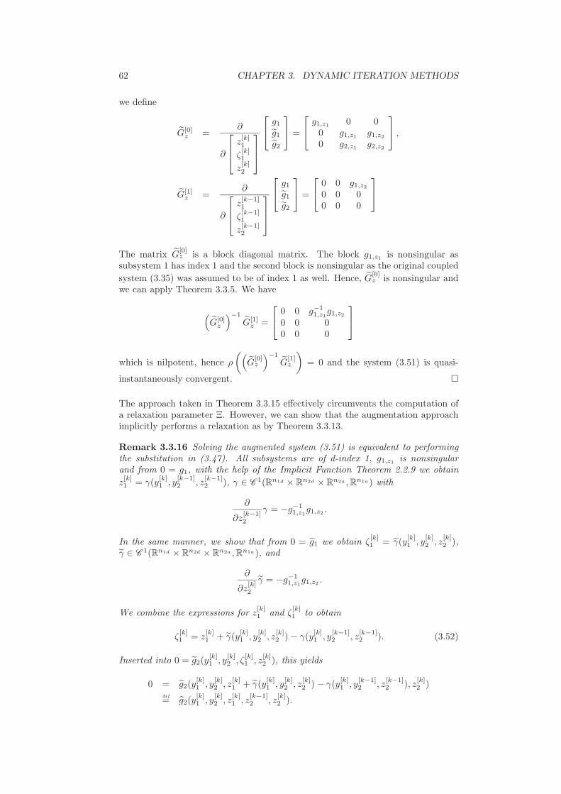
62 CHAPTER 3. DYNAMIC ITERATION METHODS
we define
G[0]z =
∂
∂
z[k]1
ζ[k]1
z[k]2
g1
g1
g2
=
g1,z10 0
0 g1,z1g1,z2
0 g2,z1g2,z2
,
G[1]z =
∂
∂
z[k−1]1
ζ[k−1]1
z[k−1]2
g1
g1
g2
=
0 0 g1,z2
0 0 00 0 0
The matrix G[0]z is a block diagonal matrix. The block g1,z1
is nonsingular assubsystem 1 has index 1 and the second block is nonsingular as the original coupled
system (3.35) was assumed to be of index 1 as well. Hence, G[0]z is nonsingular and
we can apply Theorem 3.3.5. We have
(G[0]
z
)−1
G[1]z =
0 0 g−11,z1
g1,z2
0 0 00 0 0
which is nilpotent, hence ρ
((G
[0]z
)−1
G[1]z
)= 0 and the system (3.51) is quasi-
instantaneously convergent.
The approach taken in Theorem 3.3.15 effectively circumvents the computation ofa relaxation parameter Ξ. However, we can show that the augmentation approachimplicitly performs a relaxation as by Theorem 3.3.13.
Remark 3.3.16 Solving the augmented system (3.51) is equivalent to performingthe substitution in (3.47). All subsystems are of d-index 1, g1,z1
is nonsingularand from 0 = g1, with the help of the Implicit Function Theorem 2.2.9 we obtain
z[k]1 = γ(y
[k]1 , y
[k−1]2 , z
[k−1]2 ), γ ∈ C 1(Rn1d × Rn2d × Rn2a , Rn1a) with
∂
∂z[k−1]2
γ = −g−11,z1
g1,z2.
In the same manner, we show that from 0 = g1 we obtain ζ[k]1 = γ(y
[k]1 , y
[k]2 , z
[k]2 ),
γ ∈ C 1(Rn1d × Rn2d × Rn2a , Rn1a), and
∂
∂z[k]2
γ = −g−11,z1
g1,z2.
We combine the expressions for z[k]1 and ζ
[k]1 to obtain
ζ[k]1 = z
[k]1 + γ(y
[k]1 , y
[k]2 , z
[k]2 ) − γ(y
[k]1 , y
[k−1]2 , z
[k−1]2 ). (3.52)
Inserted into 0 = g2(y[k]1 , y
[k]2 , ζ
[k]1 , z
[k]2 ), this yields
0 = g2(y[k]1 , y
[k]2 , z
[k]1 + γ(y
[k]1 , y
[k]2 , z
[k]2 ) − γ(y
[k]1 , y
[k−1]2 , z
[k−1]2 ), z
[k]2 )
def
= g2(y[k]1 , y
[k]2 , z
[k]1 , z
[k−1]2 , z
[k]2 ).

3.3. GAUSS-SEIDEL AND JACOBI METHODS 63
The system
y[k]1 = f1(y
[k]1 , y
[k−1]2 , z
[k]1 , z
[k−1]2 ),
y[k]2 = f2(y
[k]1 , y
[k]2 , z
[k]1 , z
[k]2 ),
0 = g1(y[k]1 , y
[k−1]2 , z
[k]1 , z
[k−1]2 ),
0 = g2(y[k]1 , y
[k]2 , z
[k]1 , z
[k−1]2 , z
[k]2 )
is analytically equivalent to (3.51) but the Jacobians
G[0]z =
∂
∂
[z[k]1
z[k]2
][
g1
g2
]=
[g1,z1
0g2,z1
g2,z2− g2,z1
g−11,z1
g1,z2
],
G[1]z =
∂
∂
[z[k−1]1
z[k−1]2
][
g1
g2
]=
[0 g1,z2
0 g2,z1g−11,z1
g1,z2
]
are identical to G[0]
z and G[1]
z in (3.49) with Ξ as in (3.48). Hence, the system (3.50)behaves like (3.47) and is quasi-instantaneously convergent.
Example 3.3.17 Consider a system similar to the one in Example 3.2.12:
y[k]1 = −y
[k−1]2 , (3.53a)
0 = y[k]1 + z
[k]1 − z
[k−1]2 , (3.53b)
and
y[k]2 = y
[k−1]1 , (3.54a)
0 = y[k]2 + z
[k]2 + z
[k]1 , (3.54b)
with initial values y1(0) = 1 and y2(0) = 0. The initial values for the algebraicvariables z1 and z2 cannot be prescribed and may change after each iteration. Thisis the Gauss-Seidel-DIM for the system
y1 = −y2,0 = y1 + z1 − z2,
y2 = y1,0 = y2 + z2 + z1,
(3.55)
with the solution
y1(t) = cos(t),
z1(t) = − cos(t)−sin(t)2 ,
y2(t) = sin(t),
z2(t) = cos(t)−sin(t)2 .
The differential parts (3.53a) and (3.54a) are independent of the remainder of thesystem and the iteration defined by these two equations will converge towards thecorrect solutions y1(t) = cos(t) and y2(t) = sin(t). If we set the starting iterates as
y1(t) = cos(t),
y2(t) = sin(t),
then only z1 and z2 will change in the systems (3.53) and (3.54). We can specifythe iteration as follows
z[k]1 = − cos(t) + z
[k−1]2 ,
z[k]2 = − sin(t) − z
[k]1
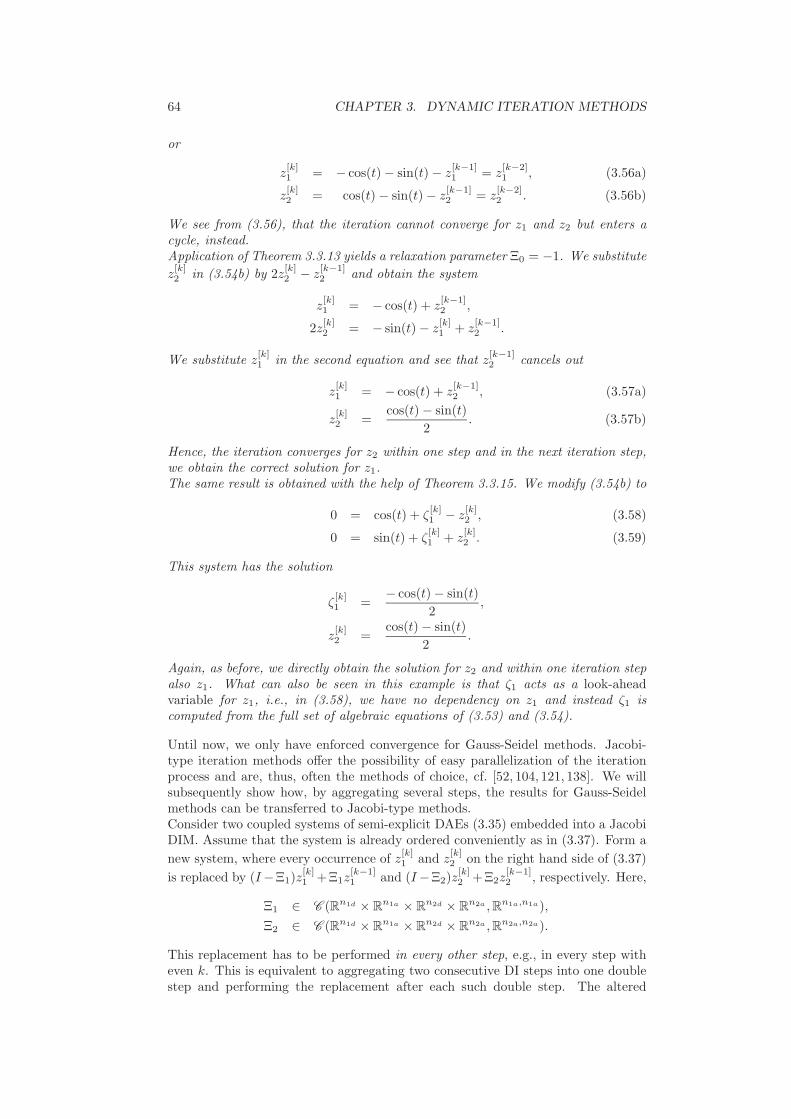
64 CHAPTER 3. DYNAMIC ITERATION METHODS
or
z[k]1 = − cos(t) − sin(t) − z
[k−1]1 = z
[k−2]1 , (3.56a)
z[k]2 = cos(t) − sin(t) − z
[k−1]2 = z
[k−2]2 . (3.56b)
We see from (3.56), that the iteration cannot converge for z1 and z2 but enters acycle, instead.Application of Theorem 3.3.13 yields a relaxation parameter Ξ0 = −1. We substitute
z[k]2 in (3.54b) by 2z
[k]2 − z
[k−1]2 and obtain the system
z[k]1 = − cos(t) + z
[k−1]2 ,
2z[k]2 = − sin(t) − z
[k]1 + z
[k−1]2 .
We substitute z[k]1 in the second equation and see that z
[k−1]2 cancels out
z[k]1 = − cos(t) + z
[k−1]2 , (3.57a)
z[k]2 =
cos(t) − sin(t)
2. (3.57b)
Hence, the iteration converges for z2 within one step and in the next iteration step,we obtain the correct solution for z1.The same result is obtained with the help of Theorem 3.3.15. We modify (3.54b) to
0 = cos(t) + ζ[k]1 − z
[k]2 , (3.58)
0 = sin(t) + ζ[k]1 + z
[k]2 . (3.59)
This system has the solution
ζ[k]1 =
− cos(t) − sin(t)
2,
z[k]2 =
cos(t) − sin(t)
2.
Again, as before, we directly obtain the solution for z2 and within one iteration stepalso z1. What can also be seen in this example is that ζ1 acts as a look-aheadvariable for z1, i.e., in (3.58), we have no dependency on z1 and instead ζ1 iscomputed from the full set of algebraic equations of (3.53) and (3.54).
Until now, we only have enforced convergence for Gauss-Seidel methods. Jacobi-type iteration methods offer the possibility of easy parallelization of the iterationprocess and are, thus, often the methods of choice, cf. [52, 104, 121, 138]. We willsubsequently show how, by aggregating several steps, the results for Gauss-Seidelmethods can be transferred to Jacobi-type methods.Consider two coupled systems of semi-explicit DAEs (3.35) embedded into a JacobiDIM. Assume that the system is already ordered conveniently as in (3.37). Form a
new system, where every occurrence of z[k]1 and z
[k]2 on the right hand side of (3.37)
is replaced by (I −Ξ1)z[k]1 +Ξ1z
[k−1]1 and (I −Ξ2)z
[k]2 +Ξ2z
[k−1]2 , respectively. Here,
Ξ1 ∈ C (Rn1d × Rn1a × R
n2d × Rn2a , Rn1a,n1a),
Ξ2 ∈ C (Rn1d × Rn1a × R
n2d × Rn2a , Rn2a,n2a).
This replacement has to be performed in every other step, e.g., in every step witheven k. This is equivalent to aggregating two consecutive DI steps into one doublestep and performing the replacement after each such double step. The altered

3.3. GAUSS-SEIDEL AND JACOBI METHODS 65
system then is of the formk odd:
y[k]1 = f1(y
[k]1 , y
[k−1]2 , z
[k]1 , z
[k−1]2 ),
y[k]2 = f2(y
[k−1]1 , y
[k]2 , z
[k−1]1 , z
[k]2 ),
0 = g1(y[k]1 , y
[k−1]2 , z
[k]1 , z
[k−1]2 ),
0 = g2(y[k−1]1 , y
[k]2 , z
[k−1]1 , z
[k]2 ),
(3.60)
k even:
y[k]1 = f1(y
[k]1 , y
[k−1]2 , (I − Ξ1)z
[k]1 + Ξ1z
[k−1]1 , z
[k−1]2 ),
y[k]2 = f2(y
[k−1]1 , y
[k]2 , z
[k−1]1 , (I − Ξ2)z
[k]2 + Ξ2z
[k−1]2 ),
0 = g1(y[k]1 , y
[k−1]2 , (I − Ξ1)z
[k]1 + Ξ1z
[k−1]1 , z
[k−1]2 ),
0 = g2(y[k−1]1 , y
[k]2 , z
[k−1]1 , (I − Ξ2)z
[k]2 + Ξ2z
[k−1]2 ).
(3.61)
The following theorem provides a convergence criterion and an optimal choice forΞ1 and Ξ2.
Theorem 3.3.18 (Enforcing the convergence of Jacobi methods)Consider a Jacobi DIM (3.60) with (3.61). If every subsystem in (3.35) is of d-index1 and the coupled system as well, then there exist relaxation parameters Ξ1 ∈ S(X0,1)and Ξ2 ∈ S(X0,2) within sufficiently small environments around
Ξ0,1 = g−11,z1
g1,z2g−12,z2
g2,z1, (3.62)
Ξ0,2 = g−12,z2
g2,z1g−11,z1
g1,z2, (3.63)
such that the DIM (3.60) and (3.61) converges to the solution of (3.35). With thechoices
Ξ1 = Ξ0,1,
Ξ2 = Ξ0,2,
the DIM (3.60) and (3.61) becomes quasi-instantaneously convergent.
Proof: We consider two consecutive iteration steps of the Jacobi DIM (3.37)together. Without loss of generality, we assume that k − 1 is odd and k is even.
y[k−1]1 = f1(y
[k−1]1 , y
[k−2]2 , z
[k−1]1 , z
[k−2]2 ),
y[k−1]2 = f2(y
[k−2]1 , y
[k−1]2 , z
[k−2]1 , z
[k−1]2 ),
y[k]1 = f1(y
[k]1 , y
[k−1]2 , z
[k]1 , z
[k−1]2 ),
y[k]2 = f2(y
[k−1]1 , y
[k]2 , z
[k−1]1 , z
[k]2 ),
0 = g1(y[k−1]1 , y
[k−2]2 , z
[k−1]1 , z
[k−2]2 ),
0 = g2(y[k−2]1 , y
[k−1]2 , z
[k−2]1 , z
[k−1]2 ),
0 = g1(y[k]1 , y
[k−1]2 , z
[k]1 , z
[k−1]2 ),
0 = g2(y[k−1]1 , y
[k]2 , z
[k−1]1 , z
[k]2 ).
(3.64)
We define
y[k] =
[y[k]1
y[k]2
]=
[y[k−1]
y[k]
]=
y[k−1]1
y[k−1]2
y[k]1
y[k]2
,
z[k] =
[z[k]1
z[k]2
]=
[z[k−1]
z[k]
]=
z[k−1]1
z[k−1]2
z[k]1
z[k]2
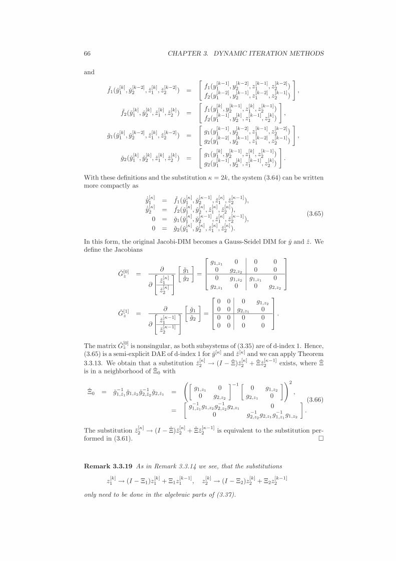
66 CHAPTER 3. DYNAMIC ITERATION METHODS
and
f1(y[k]1 , y
[k−2]2 , z
[k]1 , z
[k−2]2 ) =
[f1(y
[k−1]1 , y
[k−2]2 , z
[k−1]1 , z
[k−2]2 )
f2(y[k−2]1 , y
[k−1]2 , z
[k−2]1 , z
[k−1]2 )
],
f2(y[k]1 , y
[k]2 , z
[k]1 , z
[k]2 ) =
[f1(y
[k]1 , y
[k−1]2 , z
[k]1 , z
[k−1]2 )
f2(y[k−1]1 , y
[k]2 , z
[k−1]1 , z
[k]2 )
],
g1(y[k]1 , y
[k−2]2 , z
[k]1 , z
[k−2]2 ) =
[g1(y
[k−1]1 , y
[k−2]2 , z
[k−1]1 , z
[k−2]2 )
g2(y[k−2]1 , y
[k−1]2 , z
[k−2]1 , z
[k−1]2 )
],
g2(y[k]1 , y
[k]2 , z
[k]1 , z
[k]2 ) =
[g1(y
[k]1 , y
[k−1]2 , z
[k]1 , z
[k−1]2 )
g2(y[k−1]1 , y
[k]2 , z
[k−1]1 , z
[k]2 )
].
With these definitions and the substitution κ = 2k, the system (3.64) can be writtenmore compactly as
˙y[κ]1 = f1(y
[κ]1 , y
[κ−1]2 , z
[κ]1 , z
[κ−1]2 ),
˙y[κ]2 = f2(y
[κ]1 , y
[κ]2 , z
[κ]1 , z
[κ]2 ),
0 = g1(y[κ]1 , y
[κ−1]2 , z
[κ]1 , z
[κ−1]2 ),
0 = g2(y[κ]1 , y
[κ]2 , z
[κ]1 , z
[κ]2 ).
(3.65)
In this form, the original Jacobi-DIM becomes a Gauss-Seidel DIM for y and z. Wedefine the Jacobians
G[0]z =
∂
∂
[z[κ]1
z[κ]2
][
g1
g2
]=
g1,z10 0 0
0 g2,z20 0
0 g1,z2g1,z1
0g2,z1
0 0 g2,z2
G[1]z =
∂
∂
[z[κ−1]1
z[κ−1]2
][
g1
g2
]=
0 0 0 g1,z2
0 0 g2,z10
0 0 0 00 0 0 0
.
The matrix G[0]z is nonsingular, as both subsystems of (3.35) are of d-index 1. Hence,
(3.65) is a semi-explicit DAE of d-index 1 for y[κ] and z[κ] and we can apply Theorem
3.3.13. We obtain that a substitution z[κ]2 → (I − Ξ)z
[κ]2 + Ξz
[κ−1]2 exists, where Ξ
is in a neighborhood of Ξ0 with
Ξ0 = g−11,z1
g1,z2g−12,z2
g2,z1=
([g1,z1
00 g2,z2
]−1 [0 g1,z2
g2,z10
])2
,
=
[g−11,z1
g1,z2g−12,z2
g2,z10
0 g−12,z2
g2,z1g−11,z1
g1,z2
].
(3.66)
The substitution z[κ]2 → (I − Ξ)z
[κ]2 + Ξz
[κ−1]2 is equivalent to the substitution per-
formed in (3.61).
Remark 3.3.19 As in Remark 3.3.14 we see, that the substitutions
z[k]1 → (I − Ξ1)z
[k]1 + Ξ1z
[k−1]1 , z
[k]2 → (I − Ξ2)z
[k]2 + Ξ2z
[k−1]2
only need to be done in the algebraic parts of (3.37).
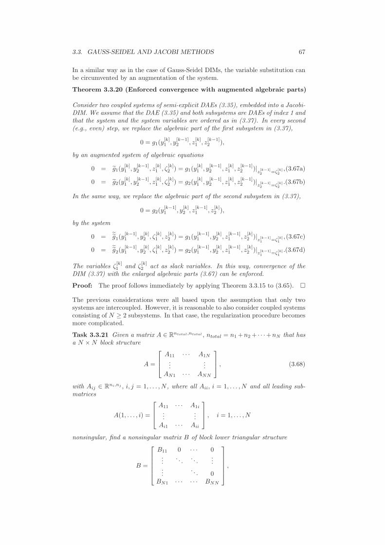
3.3. GAUSS-SEIDEL AND JACOBI METHODS 67
In a similar way as in the case of Gauss-Seidel DIMs, the variable substitution canbe circumvented by an augmentation of the system.
Theorem 3.3.20 (Enforced convergence with augmented algebraic parts)
Consider two coupled systems of semi-explicit DAEs (3.35), embedded into a Jacobi-DIM. We assume that the DAE (3.35) and both subsystems are DAEs of index 1 andthat the system and the system variables are ordered as in (3.37). In every second(e.g., even) step, we replace the algebraic part of the first subsystem in (3.37),
0 = g1(y[k]1 , y
[k−1]2 , z
[k]1 , z
[k−1]2 ),
by an augmented system of algebraic equations
0 = g1(y[k]1 , y
[k−1]2 , z
[k]1 , ζ
[k]2 ) = g1(y
[k]1 , y
[k−1]2 , z
[k]1 , z
[k−1]2 )|
z[k−1]2 =ζ
[k]2
,(3.67a)
0 = g2(y[k]1 , y
[k−1]2 , z
[k]1 , ζ
[k]2 ) = g2(y
[k]1 , y
[k−1]2 , z
[k]1 , z
[k−1]2 )|
z[k−1]2 =ζ
[k]2
.(3.67b)
In the same way, we replace the algebraic part of the second subsystem in (3.37),
0 = g2(y[k−1]1 , y
[k]2 , z
[k−1]1 , z
[k]2 ),
by the system
0 = ˜g1(y[k−1]1 , y
[k]2 , ζ
[k]1 , z
[k]2 ) = g1(y
[k−1]1 , y
[k]2 , z
[k−1]1 , z
[k]2 )|
z[k−1]1 =ζ
[k]1
,(3.67c)
0 = ˜g2(y[k−1]1 , y
[k]2 , ζ
[k]1 , z
[k]2 ) = g2(y
[k−1]1 , y
[k]2 , z
[k−1]1 , z
[k]2 )|
z[k−1]1 =ζ
[k]1
.(3.67d)
The variables ζ[k]1 and ζ
[k]2 act as slack variables. In this way, convergence of the
DIM (3.37) with the enlarged algebraic parts (3.67) can be enforced.
Proof: The proof follows immediately by applying Theorem 3.3.15 to (3.65).
The previous considerations were all based upon the assumption that only twosystems are intercoupled. However, it is reasonable to also consider coupled systemsconsisting of N ≥ 2 subsystems. In that case, the regularization procedure becomesmore complicated.
Task 3.3.21 Given a matrix A ∈ Rntotal,ntotal , ntotal = n1 +n2 + · · ·+nN that hasa N × N block structure
A =
A11 · · · A1N
......
AN1 · · · ANN
, (3.68)
with Aij ∈ Rni,nj , i, j = 1, . . . , N , where all Aii, i = 1, . . . , N and all leading sub-matrices
A(1, . . . , i) =
A11 · · · A1i
......
Ai1 · · · Aii
, i = 1, . . . , N
nonsingular, find a nonsingular matrix B of block lower triangular structure
B =
B11 0 · · · 0...
. . .. . .
......
. . . 0BN1 · · · · · · BNN
,

68 CHAPTER 3. DYNAMIC ITERATION METHODS
where with Bij ∈ Rni,nj , i = 1, . . . , N, j = 1, . . . , i, such that B−1(A − B) is nilpo-tent.
Lemma 3.3.22Consider the matrix A as in (3.68) with all properties as in Task 3.3.21. LetAT = V U be a block LU decomposition of AT without pivoting, see, e.g., [62].This decomposition always exists, since all leading submatrices were assumed to benonsingular, cf. [62, Theorem 3.2.1]. Then, B = UT is block lower triangular,nonsingular and B−1(A − B) is nilpotent.
Proof: The proof that B = UT is block lower triangular and nonsingular is trivial,given its construction from the LU-decomposition. Additionally, it also follows thatC = V T is of the block form
C =
I C12 · · · C1N
0. . .
. . ....
.... . .
. . . CN−1,N
0 · · · 0 I
,
with identical block sizes as A. With the LU-decomposition we have
AT = V U = CT BT
or A = BC. Furthermore, B−1(A − B) = B−1A − I = C − I and with the specialstructure of C, the matrix C − I is nilpotent.
The problem of finding appropriate variable substitutions z[k]i → (I−Ξ)z
[k]i +Ξz
[k−1]i
for a Gauss-Seidel DIM is related to Task 3.3.21.We consider N ≥ 2 coupled systems of semi-explicit DAEs, embedded into a Gauss-Seidel-DIM. We assume that the system is already ordered conveniently as
y[k]1 = f1(y
[k]1 , y
[k−1]2 , . . . , y
[k−1]N , z
[k]1 , z
[k−1]2 , . . . , z
[k−1]N ),
y[k]2 = f2(y
[k]1 , y
[k]2 , y
[k−1]3 , . . . , y
[k−1]N , z
[k]1 , z
[k]2 , z
[k−1]3 , . . . , z
[k−1]N ),
...
y[k]N = fN (y
[k]1 , . . . , y
[k]N , z
[k]1 , . . . , z
[k]N ),
0 = g1(y[k]1 , y
[k−1]2 , . . . , y
[k−1]N , z
[k]1 , z
[k−1]2 , . . . , z
[k−1]N ),
0 = g2(y[k]1 , y
[k]2 , y
[k−1]3 , . . . , y
[k−1]N , z
[k]1 , z
[k]2 , z
[k−1]3 , . . . , z
[k−1]N ),
...
0 = gN (y[k]1 , . . . , y
[k]N , z
[k]1 , . . . , z
[k]N ).
(3.69)
We form a new system, where every occurrence of z[k]j in gi on the right hand side
of (3.69) is replaced by (I − Ξij)z[k]j + Ξijz
[k−1]j , i = 2, . . . , N, j = 2, . . . , i, i.e.,
y[k]1 = f1(y
[k]1 , y
[k−1]2 , . . . , y
[k−1]N , z
[k]1 , z
[k−1]2 , . . . , z
[k−1]N ),
y[k]2 = f2(y
[k]1 , y
[k]2 , y
[k−1]3 , . . . , y
[k−1]N , z
[k]1 , z
[k]2 , z
[k−1]3 , . . . , z
[k−1]N ),
...
y[k]N = fN (y
[k]1 , . . . , y
[k]N , z
[k]1 , . . . , z
[k]N ),
0 = g1(y[k]1 , y
[k−1]2 , . . . , y
[k−1]N , z
[k]1 , z
[k−1]2 , . . . , z
[k−1]N ),
0 = g2(y[k]1 , y
[k]2 , y
[k−1]3 , . . . , y
[k−1]N , . . .
. . . z[k]1 , (I − Ξ22)z
[k]2 + Ξ22z
[k−1]2 , z
[k−1]3 , . . . , z
[k−1]N ),
...
0 = gN (y[k]1 , . . . , y
[k]N , z
[k]1 , (I − ΞN2)z
[k]2 + ΞN2z
[k−1]2 , . . .
. . . , (I − ΞNN )z[k]N + ΞNNz
[k−1]N ).
(3.70)

3.3. GAUSS-SEIDEL AND JACOBI METHODS 69
We set
Gz =∂
∂
z1
...zN
g1(y1, . . . , yN , z1, . . . , zN )...
gN (y1, . . . , yN , z1, . . . , zN )
=
g1,z1· · · g1,zN
......
gN,z1· · · gN,zN
.(3.71)
If all leading submatrices of Gz as in (3.71) are nonsingular, then with Lemma3.3.22, we can construct B and C as block lower and upper triangular matrices bya block LU decomposition without pivoting
Gz = BC. (3.72)
Theorem 3.3.23Consider the DIM (3.69). If a decomposition (3.72) exists and
range Bij ⊆ range gi,zj, i = 2, . . . , N, j = 2, . . . , i, (3.73)
then a set of relaxation parameters Ξij , i = 2, . . . , N, j = 2, . . . , i exists such thatthe DIM (3.70) converges to the solution of the original system of coupled semi-explicit DAEs.With the choices Ξij such that
gi,zj(I − Ξij) = Bij , i = 2, . . . , N, j = 2, . . . , i, (3.74)
the DIM (3.70) becomes quasi-instantaneously convergent.
Proof: We show that the statement holds for Ξij as in (3.74). With the continuityof the spectral radius, the assertion also holds within a neighborhood of Ξij as in(3.74).Differentiation of the algebraic part of (3.70) and application of Theorem 3.2.6 yieldsthat the DIM (3.70) is convergent if for
G[0]
z =
g1,z10 · · · 0
g2,z1g2,z2
(I − Ξ22). . .
......
.... . . 0
gN,z1gN,z2
(I − ΞN2) · · · gN,zN(I − ΞNN )
,
G[1]
z =
0 g1,z2· · · g1,zN
0 g2,z2Ξ22
. . ....
0...
. . . gN−1,zN
0 gN,z2ΞN2 · · · gN,zN
ΞNN )
,
we have
ρ((G[0]
z )−1G[1]
z ) < 1.
By construction, Gz = G[0]
z + G[1]
z and for the block LU decomposition we have
BC = Gz = G[0]
z + G[1]
z . The assumption in Equation (3.73) guarantees that (3.74)
is solvable for every Ξij , i = 2, . . . , N, j = 2, . . . , i. Hence, the matrix G[0]
z has thesame structure as B in Task 3.3.21 and with Lemma 3.3.22, it follows that
B−1(Gz − B) = (G[0]
z )−1G[1]
z
is nilpotent. With the help of Corollary 3.2.7, we have that the system (3.69) isquasi-instantaneously convergent.

70 CHAPTER 3. DYNAMIC ITERATION METHODS
Remark 3.3.24 If it is possible to change the order in which the systems are solvedthen some of the difficulties of generating appropriate relaxation parameters can beovercome. See Example 3.3.25 for an illustration of this effect.
Example 3.3.25 We consider three coupled systems of 1-dimensional algebraicequations
3z1 + z2 + z3 = 0,3z1 + 3z2 + z3 = 0,3z1 + 3z2 + 3z3 = 0,
or shorter
Gz =
3 1 13 3 13 3 3
z1
z2
z3
= 0.
As already shown in Example 3.3.8, the Gauss-Seidel method converges for thissystem with a rate of convergence of 1
3 . This rate of convergence can be acceleratedusing Theorem 3.3.23. We compute an LU decomposition GT = CT BT and obtain
B =
3 0 03 2 03 2 2
, C =
1 13
13
0 1 00 0 1
.
Theorem 3.3.23 is applicable and we obtain 3(1 − Ξij) = 2 for Ξ22, Ξ32 and Ξ33.This yields Ξij = 1
3 . Hence, the DIM
3z[k]1 + z
[k−1]2 + z
[k−1]3 = 0,
3z[k]1 + 3( 2
3z[k]2 + 1
3z[k−1]2 ) + z
[k−1]3 = 0,
3z[k]1 + 3( 2
3z[k]2 + 1
3z[k−1]2 ) + 3( 2
3z[k]3 + 1
3z[k−1]3 ) = 0
becomes quasi-instantaneously convergent. And indeed,
B−1(G − B) =
3 0 03 2 03 2 2
−1
0 1 10 1 10 1 1
=
0 13
13
0 0 00 0 0
is nilpotent.We consider a slightly different example
Gz =
3 1 13 3 13 0 3
z1
z2
z3
= 0
and compute GT = CT BT with
B =
3 0 03 2 03 −1 2
, C =
1 13
13
0 1 00 0 1
.
For this example, the range condition (3.73) is violated. We still obtain Ξ2,2 =Ξ3,3 = 1
3 but the equation 0(1−Ξ3,2) = −1 cannot be solved for Ξ3,2. In this specialcase, the situation can be resolved by exchanging the order of computation of thesecond and third subsystem. This also means, that z3 as the variable belonging tothe third subsystem is computed before z2. For this new system
Gz =
3 1 13 3 03 1 3
z1
z3
z2
= 0,

3.3. GAUSS-SEIDEL AND JACOBI METHODS 71
we can compute
B =
3 0 03 2 03 0 2
, C =
1 13
13
0 1 −12
0 0 1
.
Again, Ξ2,2 = Ξ3,3 = 13 but Ξ3,2 is arbitrary and we always obtain
B−1(G − B) =
3 0 03 2 03 0 2
−1
0 1 10 1 00 1 1
=
0 13
13
0 0 −12
0 0 0
which again is nilpotent.
Remark 3.3.26 Usually, if all combinations of subsystems form DAEs of index 1,then it will be possible to construct a decomposition of the form (3.72). Unfortu-nately, this does not guarantee the solvability of (3.74) as seen in Example 3.3.25.We have the additional freedom of reordering the subsystems. This corresponds toa symmetric permutation of Gz. Then, a different decomposition
PGzPT = BC,
where P is a block permutation matrix acting on the block structure of Gz can beobtained. So far, we are not aware of any a priori criterion that states whether aP exists such that with B, the equations (3.74) become solvable, nor do we know analgorithm that computes such a P .The problem of finding relaxation parameters as a whole remains open.
In Remark 3.3.16, we have shown that the approaches of introducing relaxationparameters, e.g., as in Theorem 3.3.13 and enlarging the algebraic part of somesubsystems as in Theorem 3.3.15 are fundamentally equivalent. This approach alsoleads to a reliable method for enforcing the convergence of N > 2 coupled systemswithin a Gauss-Seidel iteration. We consider a DIM as in (3.69). We furthermoredefine
Gzi=
gi,zi· · · gi,zN
......
gN,zi· · · gN,zN
and assume that all Gzi, i = 1, . . . , N are nonsingular. This is equivalent to the
assumption that the systems formed by coupling only subsystems i through N arestill DAEs of index 1.We form a new system with augmented algebraic parts and look-ahead-variables asfollows. We change every subsystem from
y[k]i = fi(y
[k]1 , . . . , y
[k]i , y
[k−1]i+1 , . . . , y
[k−1]N , z
[k]1 , . . . , z
[k]i , z
[k−1]i+1 , . . . , z
[k−1]N ),
0 = gi(y[k]1 , . . . , y
[k]i , y
[k−1]i+1 , . . . , y
[k−1]N , z
[k]1 , . . . , z
[k]i , z
[k−1]i+1 , . . . , z
[k−1]N )
(3.75)
to
y[k]i = fi(y
[k]1 , . . . , y
[k]i , y
[k−1]i+1 , . . . , y
[k−1]N , z
[k]1 , . . . , z
[k]i , ζ
[k]i,i+1, . . . , ζ
[k]i,N ),
0 = gi(y[k]1 , . . . , y
[k]i , y
[k−1]i+1 , . . . , y
[k−1]N , z
[k]1 , . . . , z
[k]i , ζ
[k]i,i+1, . . . , ζ
[k]i,N ),
...
0 = gN (y[k]1 , . . . , y
[k]i , y
[k−1]i+1 , . . . , y
[k−1]N , z
[k]1 , . . . , z
[k]i , ζ
[k]i,i+1, . . . , ζ
[k]i,N )
(3.76)
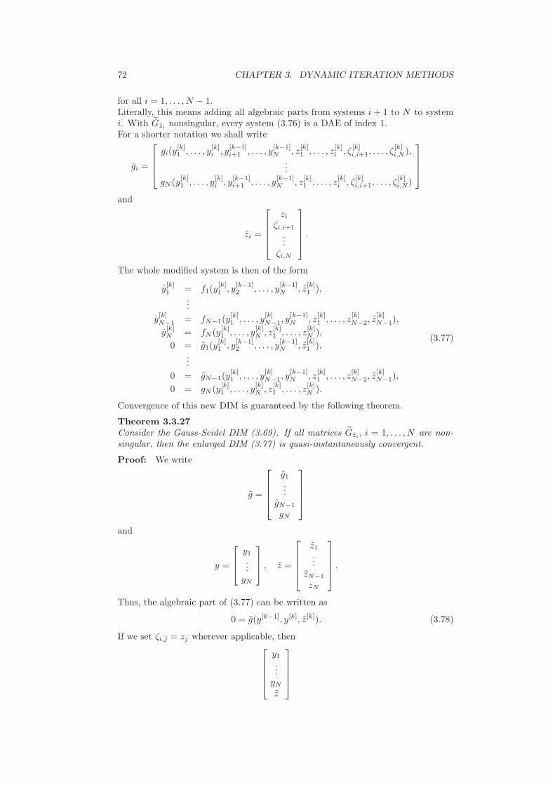
72 CHAPTER 3. DYNAMIC ITERATION METHODS
for all i = 1, . . . , N − 1.Literally, this means adding all algebraic parts from systems i + 1 to N to systemi. With Gzi
nonsingular, every system (3.76) is a DAE of index 1.For a shorter notation we shall write
gi =
gi(y[k]1 , . . . , y
[k]i , y
[k−1]i+1 , . . . , y
[k−1]N , z
[k]1 , . . . , z
[k]i , ζ
[k]i,i+1, . . . , ζ
[k]i,N ),
...
gN (y[k]1 , . . . , y
[k]i , y
[k−1]i+1 , . . . , y
[k−1]N , z
[k]1 , . . . , z
[k]i , ζ
[k]i,i+1, . . . , ζ
[k]i,N )
and
zi =
zi
ζi,i+1
...ζi,N
.
The whole modified system is then of the form
y[k]1 = f1(y
[k]1 , y
[k−1]2 , . . . , y
[k−1]N , z
[k]1 ),
...
y[k]N−1 = fN−1(y
[k]1 , . . . , y
[k]N−1, y
[k−1]N , z
[k]1 , . . . , z
[k]N−2, z
[k]N−1),
y[k]N = fN (y
[k]1 , . . . , y
[k]N , z
[k]1 , . . . , z
[k]N ),
0 = g1(y[k]1 , y
[k−1]2 , . . . , y
[k−1]N , z
[k]1 ),
...
0 = gN−1(y[k]1 , . . . , y
[k]N−1, y
[k−1]N , z
[k]1 , . . . , z
[k]N−2, z
[k]N−1),
0 = gN (y[k]1 , . . . , y
[k]N , z
[k]1 , . . . , z
[k]N ).
(3.77)
Convergence of this new DIM is guaranteed by the following theorem.
Theorem 3.3.27Consider the Gauss-Seidel DIM (3.69). If all matrices Gzi
, i = 1, . . . , N are non-singular, then the enlarged DIM (3.77) is quasi-instantaneously convergent.
Proof: We write
g =
g1
...gN−1
gN
and
y =
y1
...yN
, z =
z1
...zN−1
zN
.
Thus, the algebraic part of (3.77) can be written as
0 = g(y[k−1], y[k], z[k]). (3.78)
If we set ζi,j = zj wherever applicable, then
y1
...yN
z

3.4. CONCLUSION 73
is a fixed point of (3.77). Furthermore, the matrix
G[0]z =
∂g
∂z=
Gz10 · · · 0
∗ . . .. . .
......
. . . GzN−10
∗ · · · ∗ gN,zN
is block lower triangular and nonsingular as all its diagonal blocks were assumed tobe nonsingular. Hence, from (3.78) with the Implicit Function Theorem 2.2.9, wecan find a continuously differentiable function γ such that
z[k] = γ(y[k−1], y[k]).
We use this relation to replace all z[k]i and z
[k]i in f1 to fN and obtain a system
y[k] = f(y[k−1], y[k]). (3.79)
With Theorem 3.2.6, we have quasi-instantaneous convergence for (3.79).
Remark 3.3.28 Theorem 3.3.15 is a special case of Theorem 3.3.27 for N = 2after exchanging the order of systems 1 and 2.
3.4 Conclusion
In this Chapter, we have presented the concept of dynamic iteration for the case ofcoupled ODEs and DAEs. We have presented convergence results for both typesof equations and we have seen that there are some fundamental differences. Whilean DIM for ODEs is guaranteed to converge, a DIM for DAEs is not. Instead,we have developed a convergence criterion that is based on the computation of aspectral radius. We have specified these findings to two special forms of DIMs, theblock Jacobi- and the block Gauss-Seidel methods. For these two cases, we havealso developed different ways of transforming the DIM such that convergence ofthe method can be enforced. Especially the approach of augmenting the systemequations will be useful in the following chapter.

74 CHAPTER 3. DYNAMIC ITERATION METHODS

Chapter 4
DIM in circuit simulation
In this chapter, we will apply the theoretical results from the last chapter to DAEsarising in circuit simulation. These DAEs have a special structure, e.g., (2.30) or(2.31). Also, as we have seen in Section 2.5.3, information about spaces associatedwith the circuit DAEs can be obtained directly from the topology of the underlyingnetwork graph. In this way, numerical rank determination can be avoided in manycases. This is of special importance, since many circuit DAEs are badly scaled.Dynamic iteration for electrical circuits is a challenging task since MNA equationsare structured and splitting of these equations may destroy this structure. Wewill state an interpretation of the dynamic iteration process for electrical circuits interms of network elements. This allows a splitting of circuits on the netlist level andoffers the advantage of allowing the use of standard circuit simulation tools such as,e.g., SPICE, see Appendix C. Second, in real-life applications, MNA equations canbecome very large and analysis of these systems may become difficult because of thesize of the problems. However, the network structure behind the circuit equationscan be exploited to investigate convergence of DI methods. Also, we will give aninterpretation in terms of network topology for convergence enforcement.
4.1 Previous results
Dynamic iteration methods have been a popular simulation technique since the 80sof the twentieth century. The concept of dynamic iteration or waveform relaxation(WR) as it is often called in the context of circuit simulation has already beenemployed to a limited extend in earlier circuit simulators such as MOTIS [29], orSPLICE [113]. It was not until 1982 that the simulation program RELAX [99,100] used the capacities of DI to their full extend. The main application of DImethods was for large scale semiconductor circuits. Standard simulation tools suchas SPICE [111], use methods for stiff ODEs such as the backward Euler scheme todiscretize the circuit DAE. The resulting nonlinear algebraic system is solved foreach timestep with the help of a Newton-type iteration scheme. The computationalcost behind this approach rises dramatically with an increasing number of elementsin the circuit. The idea behind the simulators using WR is to split the circuit intosmaller subcircuits that consist of fewer elements and, thus, require less computationtime for the numerical solution. Figure 4.1 shows an example of two circuit partsthat are coupled by a resistance. The splitting of this circuit was done by cuttingthe branch from node 1 to node 2. The resistance was then duplicated to appearin both subcircuits, cf. [99]. Here, we denote the free terminals by 1′ and 2′. Thepotentials at these terminals were then prescribed by the potentials at nodes 1 and2, respectively, from the last iteration step.
75

76 CHAPTER 4. DIM IN CIRCUIT SIMULATION
21
21
1
1
2
2
1’2’
Figure 4.1: Splitting of a circuit (above) across a branch into two subcircuits (below)
G
D
S
Figure 4.2: MOS transistor
Another important aspect, especially in the context of semiconductor networks, wasthe exploitation of latency. In transistor networks, huge parts of the circuit can becompletely inactive, i.e., the voltages in these parts do not change significantly intime. With simulators such as SPICE, the nodes and elements in these parts haveto be included into discretization and computation. With an adequate splittingof the circuit, these parts become separate subcircuits and within a WR method,simulation of these latent parts has very low computational costs. Finally, manysemiconductor elements have a unidirectional voltage-current relation. This meansthat few controlling voltages control the currents in the element, while in reverse,these currents have little to no effect on the applied voltage. A typical elementwith this behaviour is a MOS circuit, where the voltage applied at the Gate (G)controls the current flow between Drain (D) and Source (S) while being almostindependent of the current itself, see also Figure 4.2. This effect, together withan adequate ordering of the subcircuits allows very efficient simulations with thehelp of WR methods. In the ensuing years, many works were published that dealtwith convergence properties of the WR method, e.g., [35, 51, 64, 65, 97] and circuitpartitioning, e.g., [3,50,52,66,110,125]. Over time, convergence criteria have becomeless restrictive. While in [99], it was necessary that every node is connected toground by a capacitance, in [35], this was only required for certain nodes. In [65], itis only required that capacitive paths and not single capacitances to ground exist.

4.2. LIST OF VARIABLES 77
Waveform relaxation has become especially interesting in the recent simulation oflumped element circuits coupled with distributed device models, cf. [104, 138].While previously, the partitioning of the circuit has often been used to achieveconvergence of the WR, we will subsequently assume, that the splitting of thecircuit is fixed. This can be the cause of, e.g., a separation of circuit elements withrespect to their type. Thus, circuit parts consisting of linear elements only may besimulated differently to parts with many nonlinear elements. In this way, modelreduction of the linear part, see, e.g., [48,114,123], may be incorporated into circuitsimulation. A splitting with respect to lumped elements and distributed elementsallows the treatment of the lumped element part with the help of standard solverssuch as SPICE while the distributed elements are simulated with specialized PDEsolvers.This separation will be discussed in the following section. Previously, often onlyRC circuits have been considered. We are going to state convergence results for arather general set of RCL circuits. Also, the methods for convergence accelerationare based on realizable circuits and not on the introduction of hypothetic elementslike negative resistances as, e.g., in [65].
4.2 List of variables
The naming of variables in this chapter follows a particular nomenclature. In orderto make it easier to understand these conventions, we will list the most frequentvariables and their use. Some notation is presented in anticipation of subsequentsections where it will be put into context.The need for lengthy subscripts on the variables arises from the need to distinguishparts of variables that have special meanings for certain subcircuits. We need todistinguish between the non-split circuit and the two subcircuits that the originalcircuit is split into. Independent from this, there is a need to distinguish the so-called C-, G- and L-subcircuits as defined in Definition 4.3.29. For potentials,we distinguish between potentials at splitting- and at non-splitting nodes. Thepotentials at splitting nodes are further separated into potentials at splitting nodeswith incident coupling current or voltage sources. The general form of a potentialvariable is
ǫκabcℓ
with the possibilities for the placeholders ǫ, κ, a, b, c and ℓ as in Table 4.1.
A similar table can be set up for variables representing currents. These have tobe distinguished by the type of element that the current flows through and by thecircuit part where that element is located. The general form of a current variable is
ικabℓ
with the possibilities for the placeholders ι, κ, a, b and ℓ as in Table 4.2.
For incidence matrices, we stick to the notation introduced in Section 2.5 with thepossibility of an ℓ subscript to distinguish which circuit is meant. The splitting ofincidence matrices into a K- and K-part, i.e., into the reduced incidence matricesfor the graph with splitting nodes only and the graph with non-splitting nodesonly is described exemplary on page 93. The newly introduced incidence matricesAKC→Rℓ, AKC→Lℓ and AKR→Lℓ follow the principle explained on page 112. Thegeneral notation of an incidence matrix is
Aabℓ

78 CHAPTER 4. DIM IN CIRCUIT SIMULATION
placeholder possibilities explanation
ǫ e: node potential in time domainE: node potential in frequency domain
κ [k]: k-th iterate in a DIMnone: for non iterated variables
a K: potential of a splitting nodeK: potential of a non-splitting node
none: if not distinguished
b C: generalized potential in bC-subcircuit
R − C: generalized potential in bG-subcircuit
L − CR: generalized potential in bL-subcircuitnone: if not distinguished
c I: potential of node with coupling I-sourceV : potential of node with coupling V-source
none: if not distinguished
ℓ 1: potential in circuit 12: potential in circuit 2
none: potential in original circuit
Table 4.1: possibilities for variable names for node potentials
placeholder possibilities explanation
ι j: current in time domainJ : current in frequency domain
κ [k]: k-th iterate in a DIMnone: for non iterated variables
a L: current through inductanceV : current through independent. V-sourceK: current through coupling V-source
none: if not distinguished
b C: coupling current in bC-subcircuit
R: coupling current in bG-subcircuit
L: coupling current in bL-subcircuitnone: if not distinguished
ℓ 1: current in circuit 12: current in circuit 2
none: current in original circuit
Table 4.2: possibilities for variable names for currents
with placeholders a, b and ℓ as in Table 4.3.
With AR =
[ARK
ARK
], this allows to define the matrix
ARℓGℓATRℓ =
[ARKℓ
ARKℓ
]Gℓ
[ARKℓ
ARKℓ
]T
=:
[GKKℓ GKKℓ
GKKℓ GKKℓ
],
for ℓ = 1, 2. Now, the matrix Gℓ is defined as
Gℓ = GKKℓ − GKKℓG−1KKℓ
GKKℓ
and it is split corresponding to the splitting eKℓ =
[eKV ℓ
eKIℓ
]
Gℓ =
[GV V ℓ GV Iℓ
GIV ℓ GIIℓ
].

4.3. GENERAL SPLITTING APPROACH 79
placeholder possibilities explanation
a R: resistive elementC: capacitive elementL: inductive elementV : voltage sourceI: current source
K: coupling source (any)none: not distinguished
b K: element incident with coupling nodeK: element not incident with coupling node
x → y: currents from bx-subcircuitto by-subcircuit, x, y ∈ C, R, L
none: if not distinguished
ℓ 1: element in circuit 12: element in circuit 2
none: element in original circuit
Table 4.3: possibilities for incidence matrices
With the help of G1 and G2, the matrices HI and HV are defined as
HI :=
[GII1 0
GV I1 + GIV 2 GII2
], HV :=
[GV V 2 GV I2 + GIV 1
0 GV V 1
].
This is the definition of the iteration matrices used to characterize convergencein the purely resistive case, see pages 93-95. In the case of RCL circuits, similarmatrices HI∗ and HV ∗ with ∗ ∈ C, G, L are constructed in exactly the same way.
4.3 General splitting approach
We want to split circuits in such a way that the circuit elements can be uniquelyassigned to one subcircuit. This was not possible with the splitting across branchesas in Figure 4.1 as there, connecting elements are duplicated. Instead, we performsplittings in the following way. We consider circuit partitionings that do not split acircuit along branches but in nodes. This allows a relatively simple interpretationof the split MNA equations in terms of netlists. The overlap that automaticallyoccurs with the splitting along branches is eliminated with the splitting in nodes.This overlap that often aids convergence of the method will be reintroduced in latersections of this chapter and exploited to accelerate the rate of convergence of thearising DI methods.
In order to specify the circuits that can be investigated, we will make the followingassumptions.
Assumption 4.3.1 We consider passive electrical networks whose graph is con-nected and that may contain the following elements:
• possibly nonlinear two-term elements (R, C, L),
• possibly nonlinear n-term elements (R, C, L),
• independent voltage and current sources,
• controlled sources that can be modelled in terms of RCL elements.
We make the further simplification that we do not allow explicit time-dependency ofRCL elements. Additionally, the nonlinearities are required to be at least Lipschitz-continuous.

80 CHAPTER 4. DIM IN CIRCUIT SIMULATION
Especially the last item poses some restrictions on the set of allowed circuits. Theexclusion of general controlled sources, e.g., as in many transistor models guaranteesa relatively simple structure of the circuit DAE and will be helpful for a laterconvergence analysis.Under these assumptions, the MNA equations (2.31) can be written as
ACC(ATCe)AT
C
d
dte + ARG(AT
Re)ATRe + ALjL + AV jV + AI i(t) = 0, (4.1a)
ATLe − L(jL)
d
dtjL = 0, (4.1b)
ATV e − v(t) = 0. (4.1c)
We intend to split this circuit in order to be able to treat the arising subcircuitsseparately with common circuit simulators or solvers especially tailored to specificelements, e.g., solvers for semiconductor device models, cf. [21,33,119,130]. To thisend, it is imperative that after the splitting process, the arising subcircuits togetherwith the means of exchanging data between them are again valid circuits.This can be accomplished by the introduction of coupling source pairs.
Definition 4.3.2 (duplicated nodes, identified nodes)
• Let G(N, B) be the graph of a circuit. Let BI0(n) be the set of all branchesthat are incident with n. A duplication of a node n is a transformation of thecircuit graph where a new node n′ is introduced. With this transformation, thebranches that were originally incident with n may be distributed freely betweenn and n′ such that
BI(n) ∪ BI(n′) = BI0(n), and BI(n) ∩ BI(n
′) = ∅,
where BI(n) and BI(n′) are the sets of branches that are incident with n and
n′, respectively, after the transformation. All other nodes and incidence rela-tions remain unchanged. See Figure 4.3.
• Let n and n′ be two nodes of a circuit. If a perfect short circuit is put betweenthese nodes, i.e., they are connected such that the potential at both nodes isidentical, we call these nodes identified.
Definition 4.3.3 (coupling source pair)Consider an electrical circuit and two nodes n and n′ of that circuit. Let e ande′ be the node potentials at n and n′, respectively. Assume that there is a voltagesource from n′ to ground that sets the potential e′ = e. Let the current through thisvoltage source be denoted jK and assume that there is a current source from groundto n that introduces jK into n. Then, we call these two sources coupling source pair.
Lemma 4.3.4Consider a circuit with graph G(N, B). Let G′(N′, B′) be the graph that arises withthe duplication of n into n and n′. Let these two nodes be connected via a couplingsource pair. Then, the circuits described by G and G′ have identical potentials fornodes in N, and identical branch currents.

4.3. GENERAL SPLITTING APPROACH 81
n
n
n′
b1b1
b2b2
b3b3
b4b4
b5b5
b6b6
Figure 4.3: node with incident branches (left), duplicated nodes with distributedbranches (right)
Proof: We use the MNA equations (2.31) to determine node potentials and branchcurrents. The KCL equations for the circuits defined by G(N, B) and G′(N′, B′)are identical, except for the nodes n, n′ and all nodes incident with any of thesetwo nodes. From the definition of the voltage source in the source pair, it is clearthat the potentials at both nodes are identical. Hence, the node potentials at n
and n′ are exchangeable and the KCL equations for all nodes incident with n or n′
are equivalent in G(N, B) and G′(N′, B′). The same is valid for any application ofKirchhoff’s Voltage Law (KVL) involving either node. Hence, the MNA equationsfor G(N, B) and G′(N′, B′) are equivalent with one exception. The KCL equationfor n in G(N, B) is replaced by two KCL equations for n and n′ in G′(N′, B′).We apply KCL to n in G′(N′, B′),
nel−1∑
ℓ=1
jℓ − iK = 0. (4.2)
Here, nel is the number of currents flowing into or out of the node and jℓ are therespective currents, not counting the current source of the coupling source pair.The current coming from that source is iK and it is directed towards n. At n′,Kirchhoff’s Current Law (KCL) yields
n′
el−1∑
ℓ=1
j′ℓ + jK = 0, (4.3)
where n′el is the number of currents flowing into or out of n′ and j′ℓ are the respective
currents, not counting the current through the voltage source of the coupling sourcepair. The voltage source is directed away from n′, hence the current jK appears
e e′
n n′
v = eiK = jK
jK
Figure 4.4: coupling source pair

82 CHAPTER 4. DIM IN CIRCUIT SIMULATION
111 222
eee e′
v = e v = eiK = jKiK = jK
jK jK
Figure 4.5: left: original circuit, center: pre-splitting circuit, right: split circuit
with a positive sign. From (4.3), we obtain that
jK = −n′
el−1∑
ℓ=1
j′ℓ.
With the definition of the coupling source pair, we have iK = jK and inserting thisexpression into (4.2) yields
nel−1∑
ℓ=1
jℓ +
n′
el−1∑
ℓ=1
j′ℓ = 0.
This is KCL applied to a circuit, where n and n′ are identified. Hence, the MNAequations for G(N, B) and G′(N′, B′) are equivalent. Thus, node potentials atcorresponding nodes and branch currents through corresponding branches are iden-tical.
In contrast to other approaches, e.g., in [97], we do not split the circuit alongbranches, but by duplicating certain nodes.
Definition 4.3.5 (splitting nodes, split circuit)
• We call a node of a circuit, that has been duplicated and where a couplingsource pair exists between both nodes a pair of splitting nodes or pair of cou-pling nodes.
• If a circuit can be partitioned into subcircuits such that there is no path oronly paths passing through the ground node from one subcircuit to another,then we call it a split circuit.
• A circuit, where some nodes have only been designated for splitting but not yetduplicated and where both sources of a coupling source pair are incident witheach of these nodes will be called a pre-splitting circuit.
For an illustration of Definition 4.3.5, see Figure 4.5.Lemma 4.3.4 guarantees that all three circuits depicted in Figure 4.5 behave identi-cally, i.e., all currents and voltages that appear in the original circuit have the samevalue in the two other circuits.For simplification, in the following we will only consider the splitting of circuits intotwo separate subcircuits. Consequently, we will refer to the subcircuits arising fromthe node-splitting as subcircuits 1 and 2 or simply as circuits 1 and 2. By iteratingthe approach, a circuit can be split into an arbitrary number of subcircuits.We will first consider the original circuit with a set of designated splitting nodes.We introduce a coupling source pair to each of these nodes, but without duplicating

4.3. GENERAL SPLITTING APPROACH 83
these nodes. In that way, we introduce a special set of voltage and current sourcesinto the network. The incidence matrix of the current and voltage sources is iden-tical, as two sources always go from ground to the designated splitting nodes. Thisincidence matrix will be denoted by AK . With an appropriate ordering of the nodepotentials of the circuit as
e =
[eK
eK
],
where eK are the potentials at designated splitting nodes and eK the potentials ofthe remaining nodes, one has
AK =
[InK
0
],
where nK is the number of designated splitting nodes. The MNA equations of thearising pre-splitting circuit can be written as follows
ACC(ATCe)AT
C
d
dte + ARG(AT
Re)ATRe + ALjL + AV jV + AI i(t)+
+AKjK = AKjK , (4.4a)
ATLe − L(jL)
d
dtjL = 0, (4.4b)
ATV e − v(t) = 0, (4.4c)
ATKe = AT
Ke. (4.4d)
Here, we have already used the definition of the currents iK of the current sourcesin the coupling source pair as iK = jK . Also, the change of structure comparedto the MNA equations (4.1) is deliberate. To go from a pre-splitting circuit to asplit circuit is rather obvious. The topology of the arising subcircuits is mostlydetermined by the choice of splitting nodes. The coupling between the subcircuitsis accomplished by the coupling sources. Only one source is assigned to each node ofthe splitting node pair. The only freedom is to which part which source is assigned.See also Figure 4.6. This freedom of choice can be used for several effects as we willsee in subsequent sections. However, there are additional restrictions to the waythe sources are assigned. These further restrictions arise from KCL and KVL andforbid that there are cutsets of current sources or loops of voltage sources.
Convention 4.3.6 In order to keep graphical circuit representations simple, weintroduce a curved dashed arc to represent a coupling source pair. The head of thearc always points to the voltage source and the tail originates in the current source.
Definition 4.3.7 (consistent source assignment)An assignment of the sources of coupling source pairs has to fulfill the followingthree criteria to be called consistent:
(a) The two sources forming a source pair cannot be part of the same subcircuit.
(b) The voltage source of a source pair cannot be placed in such a way that itforms a loop with existing voltage sources.
(c) The current source of a source pair cannot be placed in such a way that itforms a cutset with existing current sources.
Remark 4.3.8 It is possible but not advisable to choose a node incident with abranch of a voltage source that is grounded as a splitting node. This may cause a
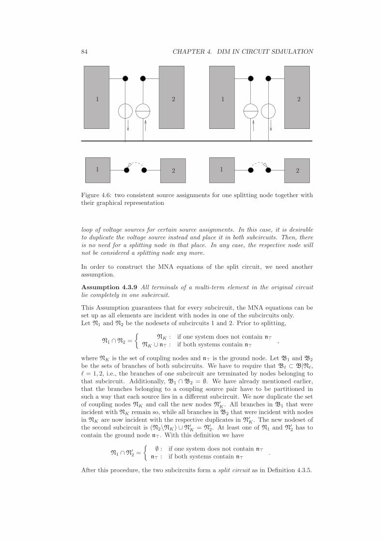
84 CHAPTER 4. DIM IN CIRCUIT SIMULATION
11
11
22
22
Figure 4.6: two consistent source assignments for one splitting node together withtheir graphical representation
loop of voltage sources for certain source assignments. In this case, it is desirableto duplicate the voltage source instead and place it in both subcircuits. Then, thereis no need for a splitting node in that place. In any case, the respective node willnot be considered a splitting node any more.
In order to construct the MNA equations of the split circuit, we need anotherassumption.
Assumption 4.3.9 All terminals of a multi-term element in the original circuitlie completely in one subcircuit.
This Assumption guarantees that for every subcircuit, the MNA equations can beset up as all elements are incident with nodes in one of the subcircuits only.Let N1 and N2 be the nodesets of subcircuits 1 and 2. Prior to splitting,
N1 ∩ N2 =
NK : if one system does not contain n⊤
NK ∪ n⊤ : if both systems contain n⊤,
where NK is the set of coupling nodes and n⊤ is the ground node. Let B1 and B2
be the sets of branches of both subcircuits. We have to require that Bℓ ⊂ B|Nℓ,ℓ = 1, 2, i.e., the branches of one subcircuit are terminated by nodes belonging tothat subcircuit. Additionally, B1 ∩ B2 = ∅. We have already mentioned earlier,that the branches belonging to a coupling source pair have to be partitioned insuch a way that each source lies in a different subcircuit. We now duplicate the setof coupling nodes NK and call the new nodes N′
K . All branches in B1 that wereincident with NK remain so, while all branches in B2 that were incident with nodesin NK are now incident with the respective duplicates in N′
K . The new nodeset ofthe second subcircuit is (N2\NK) ∪ N′
K = N′2. At least one of N1 and N′
2 has tocontain the ground node n⊤. With this definition we have
N1 ∩ N′2 =
∅ : if one system does not contain n⊤
n⊤ : if both systems contain n⊤.
After this procedure, the two subcircuits form a split circuit as in Definition 4.3.5.

4.3. GENERAL SPLITTING APPROACH 85
Definition 4.3.10 (selector matrices)Let N be the ordered set of nodes of a pre-splitting circuit. Let N1 and N2 be theordered sets of nodes of subcircuits 1 and 2. We define matrices S1 and S2 asfollows. Let nℓ = |Nℓ| be the number of nodes in subcircuit ℓ = 1, 2, then
Sℓ =[
s1 · · · snℓ
],
where sp is the qth unit vector of size N = |N| if the pth node in Nℓ is the qth nodein N.
Example 4.3.11 A circuit contains four nodes N = n1, n2, n3, n4. The noden2 is a designated splitting node and the remaining nodes are assigned such thatsubcircuit 1 has nodeset N1 = n1, n2, n4 and subcircuit 2 has N2 = n2, n3.For a number of reasons, it can be desirable to change the ordering of these nodes.Usually, we need to sort splitting nodes first. Assuming that the remaining nodesare in ascending order, we obtain for the ordered nodeset N1 = n2, n1, n4, whileN2 remains as it is. With the above definitions, for this specific example we obtain
S1 =
0 1 01 0 00 0 00 0 1
, S2 =
0 01 00 10 0
.
Let e be the vector of node potentials in the original circuit. Let e1 and e2 be thevector of node potentials in the first and second subcircuit, respectively. With thisdefinition
eℓ = STℓ e and ST
ℓ Sℓ = Inℓ, ℓ = 1, 2. (4.5)
Additionally, we can express the fact that the node potentials at coupling nodes areidentical in both subcircuits by the relations
ATK1e1 = AT
K1ST1 S2e2,
ATK2e2 = AT
K2ST2 S1e1,
where AK1 and AK2 are the incidence matrices with respect to coupling voltagesources in subcircuit 1 and 2, respectively.For each subcircuit, we can now set up the MNA equations, as described earlier.Let jLℓ, jV ℓ, jKℓ, iℓ with ℓ = 1, 2 be the currents through inductances, indepen-dent sources, coupling sources and current sources in both subcircuits. Let Cℓ, Gℓ
and Lℓ with ℓ = 1, 2 be the capacitance, conductance and inductance matrices insubcircuit ℓ, respectively. Finally, let vℓ, ℓ = 1, 2 be the voltage across independentvoltage sources in each subcircuit. Let Aℓ = [ACℓ, ARℓ, ALℓ, AV ℓ, AIℓ, AKℓ] be theelement-related incidence matrices as in (4.4). With these conventions, the MNAequations for the two subcircuits are
AC1C1(ATC1e1)A
TC1
d
dte1 + AR1G1(A
TR1
e1)ATR1
e1 + AL1jL1 + AV 1jV 1 + AI1i1(t)+
+AK1jK1 = ST1 S2AK2jK2, (4.6a)
ATL1e1 − L1(jL1)
d
dtjL1 = 0, (4.6b)
ATV 1e1 − v1(t) = 0, (4.6c)
ATK1e1 = AT
K1ST1 S2e2, (4.6d)

86 CHAPTER 4. DIM IN CIRCUIT SIMULATION
for the first subcircuit and
AC2C2(ATC2e2)A
TC2
d
dte2 + AR2G2(A
TR2
e2)ATR2
e2 + AL2jL2 + AV 2jV 2 + AI2i2(t)+
+AK2jK2 = ST2 S1AK1jK1, (4.7a)
ATL2e2 − L2(jL2)
d
dtjL2 = 0, (4.7b)
ATV 2e2 − v2(t) = 0, (4.7c)
ATK2e2 = AT
K2ST2 S1e1 (4.7d)
for the second subcircuit. Using Lemma 4.3.4, we have that integration of (4.4)yields the same solution as (4.6) and (4.7) together.However, in the formulation (4.6) and (4.7), it is easy to apply a Dynamic Iterationmethod and interpret the result as a circuit. Consider the Gauss-Seidel methodapplied to (4.6) and (4.7). We obtain
AC1C1(ATC1e
[k]1 )AT
C1
d
dte[k]1 + AR1G1(A
TR1e
[k]1 )AT
R1e[k]1 + AL1j
[k]L1+
+AV 1j[k]V 1 + AI1i1(t) + AK1j
[k]K1 = ST
1 S2AK2j[k−1]K2 , (4.8a)
ATL1e
[k]1 − L1(j
[k]L1)
d
dtj[k]L1 = 0, (4.8b)
ATV 1e
[k]1 − v1(t) = 0, (4.8c)
ATK1e
[k]1 = AT
K1ST1 S2e
[k−1]2 , (4.8d)
AC2C2(ATC2e
[k]2 )AT
C2
d
dte[k]2 + AR2G2(A
TR2e
[k]2 )AT
R2e[k]2 + AL2j
[k]L2+
+AV 2j[k]V 2 + AI2i2(t) + AK2j
[k]K2 = ST
2 S1AK1j[k]K1, (4.9a)
ATL2e
[k]2 − L2(j
[k]L2)
d
dtj[k]L2 = 0, (4.9b)
ATV 2e
[k]2 − v2(t) = 0, (4.9c)
ATK2e
[k]2 = AT
K2ST2 S1e
[k]1 . (4.9d)
Note that the matrices ST2 S1AK1 and ST
1 S2AK2 also are incidence matrices. Morespecifically, as every coupling voltage source in one subcircuit corresponds to acoupling current source at the duplicate node in the other subcircuit, they are theincidence matrices of the coupling current sources in each subcircuit. The terms
ST1 S2AK2j
[k−1]K2 and ST
2 S1AK1j[k]K1 in Equations (4.8a) and (4.9a) can be regarded
as standard independent current sources because at the time of computation of the
respective subsystem, the progression of j[k−1]K2 or j
[k]K1 is already known. The same
is valid for ATK1S
T1 S2e
[k−1]2 and AT
K2ST2 S1e
[k]1 in Equations (4.8d) and (4.9d) that
can be treated like standard independent voltage sources. This makes it rather easyto implement the split circuit with standard circuit simulation tools such as, e.g.,SPICE [112].
Observation 4.3.12 Consider a coupled system of the form
f1(x1, x2) = h1(t),
f2(x1, x2) = h2(t).
Applying the Gauss-Seidel DIM to this system yields
f1(x[k]1 , x
[k−1]2 ) = h1(t),
f2(x[k]1 , x
[k]2 ) = h2(t).

4.3. GENERAL SPLITTING APPROACH 87
With the help of the Implicit Function Theorem 2.2.9 and the Banach Fixed PointTheorem 2.2.5, we see that convergence of this problem solely depends onρ(f−1
1,x1f1,x2
f−12,x2
f2,x1). The inhomogeneities h1 and h2 do not influence the overall
convergence behaviour. Hence, it may be simpler to only consider the homogeneousproblem
f1(x[k]1 , x
[k−1]2 ) = 0,
f2(x[k]1 , x
[k]2 ) = 0.
The same is valid, if not algebraic but differential-algebraic equations
F1(x[k]1 , x
[k]1 , x
[k−1]2 ) = h1(t),
F2(x[k]2 , x
[k]1 , x
[k]2 ) = h2(t)
are considered, see Corollary 3.2.8.As a consequence, in Equations (4.8a) and (4.9a), we may assume i1(t) = 0 andi2(t) = 0, without changing the convergence behaviour of the dynamic iterationmethod. For the same reason, we can assume v1(t) = 0 and v2(t) = 0 in (4.8c)(4.9c). Setting the currents i1 and i2 to zero is equivalent to just removing thecorresponding branches from the network. If we set v1 to zero, then Equation (4.8c)becomes
ATV 1e
[k]1 = 0.
This implies that the potential of nodes incident with a voltage source is identical.Hence, these nodes can be identified. As a consequence, we can contract all indepen-dent voltage sources and remove all independent current sources without changingthe convergence behaviour of the DIM. If by such a contraction two or more distinctcoupling nodes fall together, then they are treated as one node and only one couplingsource pair is incident with this node.
Dynamic Iteration methods are typically applied in a macro step which is larger thanthe average step size of numerical integration methods, but if necessary, smaller thanthe complete time interval of interest. This and the assumption that the behaviourof nonlinear elements is at least Lipschitz-continuous gives us the freedom to choosethe macro step size in such a way, that the nonlinear elements can be assumed moreor less linear on the macro step. With all these simplifications, we will only considercircuits that satisfy the following conditions.
Assumption 4.3.13 We consider split circuits consisting of two subcircuits. Thecircuits contains only:
• constant n-term resistances, capacitances and inductances (n ≥ 2),
• coupling sources (only one in each coupling node).
The matrices Cℓ, Gℓ and Lℓ, ℓ = 1, 2 are assumed to have positive definite symmetricparts.
This assumption is a refinement of Assumption 4.3.1 and only needed for conver-gence analysis. The removal of independent sources is motivated by Observation4.3.12. The consideration of linear elements only allows to perform a concise analy-sis of the convergence behaviour of the DIM (4.8) with (4.9) on a sufficiently smallmacro step with tools from linear algebra. Hence, for a local convergence analysisof a circuit that fulfills Assumption 4.3.1, after splitting the circuit, it is sufficientto investigate circuits fulfilling Assumption 4.3.13.

88 CHAPTER 4. DIM IN CIRCUIT SIMULATION
We will subsequently try to find criteria when DIM systems of the form (4.8) and(4.9) converge to a solution. More importantly, we will be interested in constel-lations of coupling source pairs that make the DIM convergent. Depending onthe placement of the coupling sources in either subcircuit, the systems (4.8) and(4.9) change. There are 2nK different possibilities for the placement of the cou-pling sources, where nK is the number of coupling nodes. So, we will be especiallyinterested in methods that find good source assignments without testing all 2nK
possibilities.
4.3.1 The purely resistive case
The main topic of this section is to determine whether Gauss-Seidel dynamic iter-ation methods work for circuits with MNA equations of the form
ARGATRe + AV jV + is(t) = 0, (4.10a)
ATV e = v(t). (4.10b)
The respective DI equations are of the form
AR1G1ATR1e
[k]1 + AV 1e
[k]1 + AK1j
[k]K1 + is1(t) = ST
1 S2AK2j[k−1]K2 , (4.11a)
ATV 1e1 = v1(t), (4.11b)
ATK1e
[k]1 = AT
K1ST1 S2e
[k−1]2 , (4.11c)
AR2G2ATR2e
[k]2 + AV 2e
[k]2 + AK2j
[k]K2 + is2(t) = ST
2 S1AK1j[k]K1, (4.12a)
ATV 2e2 = v2(t), (4.12b)
ATK2e
[k]2 = AT
K2ST2 S1e
[k]1 . (4.12c)
With Observation 4.3.12, we know that the convergence behaviour of the DIM (4.11)and (4.12) does not change if branches containing independent voltage sources arecontracted and branches with independent current sources are omitted. In order tostudy (4.10), we define an auxiliary system
ARGATRe = 0, (4.13)
by contracting branches with voltage sources and removing current sources. Thecircuit (4.10) fulfills Assumption 4.3.1. For a convergence analysis on a short macro
step, it is sufficient to consider (4.13). The distinguishment between G and G, AR
and AR as well as e and e in Equations (4.10) and (4.13) is done to show, thatthe corresponding circuit equations are fundamentally different. By contractingbranches of voltage sources, some resistances are contracted as well and incidentnodes do not have two distinct potentials but only one. Also, as eℓ changes to eℓ,then so does AKℓ to AKℓ. Hence, (4.10) and (4.13) have different solutions butwith Observation 4.3.12, on short macro steps, they have comparable convergencebehaviour. A convergence analysis of (4.13) is considerably easier than for (4.10).
We assume that symm G is positive definite and that AR has full rank. Under theseassumptions, the solution e of (4.13) is unique and trivial. Also, all splittings of(4.13) fulfill Assumption 4.3.13.The considered circuits do not contain dynamic elements, i.e., no capacitances andinductances. This is indeed a severe restriction on the set of possible circuits. How-ever, in Section 4.3.2 we will see that the techniques used to analyze the networksand convergence of the DIM also apply to the more general RCL networks. For
4.3. GENERAL SPLITTING APPROACH 89
the remainder of this subsection, we will only consider systems of the form (4.13).We split the circuit along given splitting nodes and appropriately assign couplingsources. After application of the Gauss-Seidel method, the systems of the dynamiciteration method have the form
AR1G1ATR1e
[k]1 + AK1j
[k]K1 = ST
1 S2AK2j[k−1]K2 , (4.14a)
ATK1e
[k]1 = AT
K1ST1 S2e
[k−1]2 , (4.14b)
AR2G2ATR2e
[k]2 + AK2j
[k]K2 = ST
2 S1AK1j[k]K1, (4.15a)
ATK2e
[k]2 = AT
K2ST2 S1e
[k]1 . (4.15b)
Convergence of the systems (4.14) and (4.15) will mean that e[k]1 and e
[k]2 converge
to zero for k → ∞. This will also imply that in the iteration (4.11) and (4.12), e[k]1
and e[k]2 converge to the respective node potentials in e for the more complicated
system (4.10).Each of the systems (4.14) and (4.15) is an algebraic equation for the unknown
pair
[e[k]ℓ
j[k]Kℓ
]. The solvability of the linear systems depends on the topology of the
network and can be characterized as follows.
Lemma 4.3.14 (solvability criterion)The MNA systems (4.14) and (4.15) are uniquely solvable if symm (Gℓ), ℓ = 1, 2,is positive definite and if every node is connected to the ground node by a pathconsisting of branches occupied by a resistance or a coupling voltage source only.
Proof: The criterion for the solvability of circuit equations for linear circuits withnon-dynamic elements is well documented in the literature. See, e.g., [36].
Remark 4.3.15 The converse of Lemma 4.3.14 is not true. The most commoncounterexample is a circuit with a tunnel diode, cf. [30]. For certain bias voltages,tunnel diodes have a negative conductance value and thus, the matrix symm(G)becomes indefinite while the circuit equations may still be uniquely solvable.
We will assume that the vector of node potentials eℓ is ordered in such a way thatthe node potentials eKV ℓ of coupling nodes with a coupling voltage source are thefirst entries, followed by the node potentials eKIℓ of nodes with a coupling currentsource, with the remaining potentials eKℓ at the end,
eℓ =
eKV ℓ
eKIℓ
eKℓ
. (4.16)
With this ordering of the node potentials, we have
AKℓ =
[InKV ℓ
0
],
where in contrast to earlier definitions nKV ℓ is the number of voltage sources be-longing to coupling source pairs in each subcircuit. For further simplification, weassume that the coupling nodes with coupling voltage sources in subcircuit 1 areordered identically to the coupling nodes with coupling current sources in subcircuit

90 CHAPTER 4. DIM IN CIRCUIT SIMULATION
2 and analogously for the coupling nodes with current sources in subcircuit 1 andnodes with voltage sources in subcircuit 2. With this,
ST1 S2 =
0 InKV 10
InKV 20 0
0 0 0
.
We have assumed that in each subcircuit, every node is connected to ground viabranches with resistances or coupling voltage sources. The potential at any nodethat is not grounded in this way cannot be determined by means of coupling voltagesor currents and can, thus, be left out of further considerations. Going even further,we can require that every node belongs to a block that also contains a branchoccupied by a coupling source. The following theorem characterizes relevant nodesand branches in a graph theoretical way.
Definition 4.3.16 (relevant branches, relevant nodes)We call a branch relevant if leaving that branch out of the network changes theconvergence behaviour of the DIM. A node is relevant if and only if it is incidentwith a relevant branch.
This definition translates to: Branches whose current is independent of currentsflowing into coupling nodes, are not relevant. All other branches are. In this way, theremoval of a non-relevant node together with all branches incident with it removesonly non-relevant branches.
Theorem 4.3.17 (relevant branches, relevant nodes)Only branch currents and node potentials belonging to branches and nodes that liein a block with a coupling source branch are relevant.
Proof: For simplicity, we only consider subsystem 1. Take Equation (4.14a),
where we set j[k]R1 = G1A
TR1e
[k]1 . Written slightly different, it takes the form
AR1j[k]R1 + AK1j
[k]K1 + ST
1 S2AK2(−j[k−1]K2 ) = 0. (4.17)
The currents j[k]K1 are caused by the coupling voltage sources in the subcircuit.
Equation (4.17) would not change, if instead of voltage sources, there were identi-
cally directed current sources in the circuit that generate the currents j[k]K1. We set
AK1 = [AK1, ST1 S2AK2] and j
[k]K1 =
[j[k]K1
−j[k−1]K2
]and obtain
AR1j[k]R1 + AK1j
[k]K1 = 0. (4.18)
If the node potentials in e1 are ordered as in (4.16), then
AK1 =
InKV 10
0 InKV 2
0 0
.
We first want to characterize all solutions of (4.18). The task is to find all vectors in
ker[AR1, AK1]. This can be done with the help of Lemma 2.4.28, where it is statedthat the kernel of an incidence matrix A is spanned by the vectors of fundamentalloops of the graph. Hence, every solution of (4.18) is a linear combination of loopvectors.We consider the graph G(N, B) of subcircuit 1. We construct a tree T(NT , BT ) inthis graph that contains all branches occupied by coupling sources. This is always

4.3. GENERAL SPLITTING APPROACH 91
possible, as there are no loops of coupling sources in the circuit. Let M be thefundamental loop matrix of G with respect to the tree T. With Theorem 2.4.31, wehave that M is of the form
M =[
I MRT MKT
].
The submatrix MRT contains entries if resistive branches in T are contained in aloop and MKT has entries where branches with coupling sources appear in loops.The leading identity matrix represents connecting branches that close unique loopswith the remaining tree branches. We order M in such a way that rows representingthe loops containing a coupling source appear first, followed by the remaining loops.With an appropriate ordering of branches, M takes the form
M =
[MK
MK
]=
[I 0 MK
RT 0 MKKT
0 I 0 MK
RT 0
].
The special structure of this matrix is due to the properties of 2-connected com-ponents, see Theorem 2.4.16. Here, MK is the fundamental loop matrix for the
subgraph of all blocks containing coupling sources and MK
is the fundamental loopmatrix for the subgraph of all remaining blocks. The five columns of M representthe branches of G in the order of:
1. connecting branches in blocks with coupling sources,
2. connecting branches in blocks without coupling sources,
3. tree branches in blocks with coupling sources,
4. tree branches in blocks without coupling sources,
5. branches with coupling sources.
From the properties of blocks, there are no branches with coupling sources in any
loop described by MK
and the respective entries of MKT are zero. Analogously,the splitting of the loops with respect to blocks with or without coupling sourcesinduces a block structure for MRT . A tree branch that lies in a loop that is closedby a connecting branch not lying in a block with a coupling source cannot be partof a loop with a coupling source. With the same argumentation, a tree branch thatis part of a loop with a connecting branch in a block with a coupling source itselfalways lies in a loop with such a source. Therefore, it cannot at the same time lie
in a loop described by MK
. With this argumentation, the respective blocks in MK
and MK
are empty.This separation of loops also induces a decomposition of ker[AR1, AK1] into ortho-
gonal subspaces. The only solutions of (4.18) that depend on the currents j[k]K1 are
the vectors
[j[k]R1
j[k]K1
]that lie in ker MK . With the structure of MK , this implies that
only branch currents of branches that lie in blocks with coupling source branchescan be influenced by the source currents. Conversely, a branch that does not lie ina block with a coupling source branch cannot carry a current that can be influencedby a source current. From the definition of relevant nodes we have that relevantnodes are incident with relevant branches and therefore have to be nodes of blockswith coupling source branches.
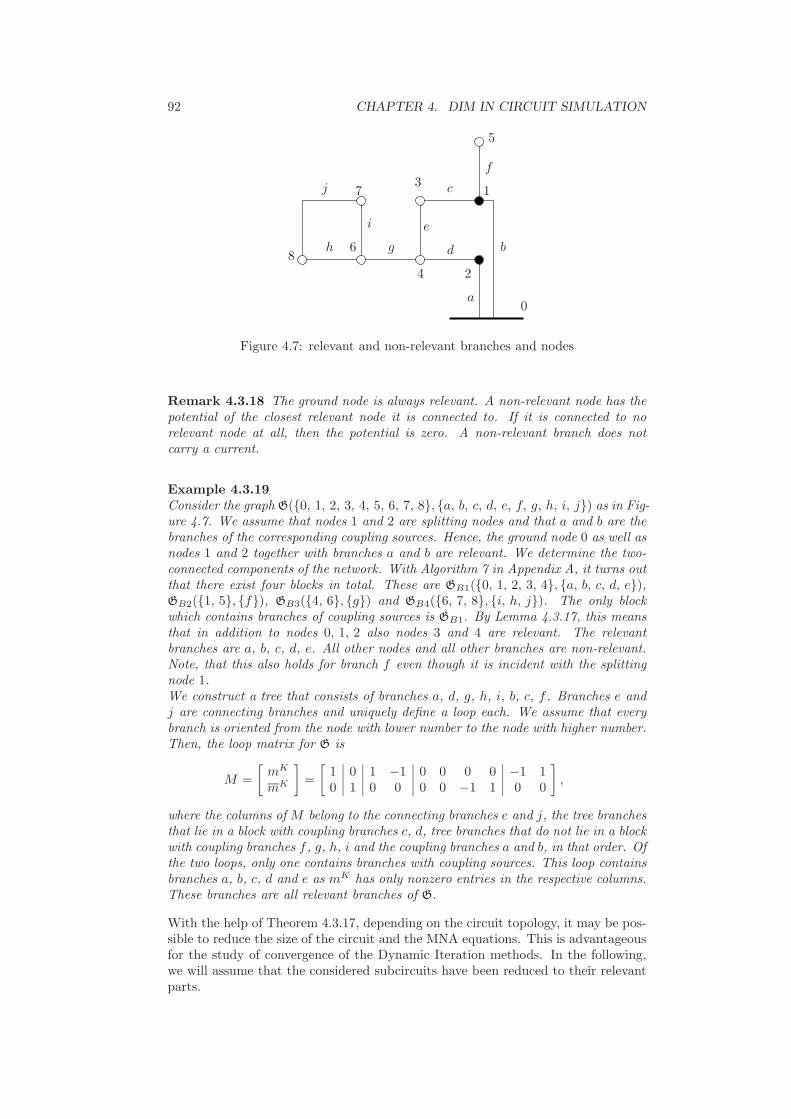
92 CHAPTER 4. DIM IN CIRCUIT SIMULATION
b
a
c
d
e
f
gh
i
j
0
1
2
3
4
5
6
7
8
Figure 4.7: relevant and non-relevant branches and nodes
Remark 4.3.18 The ground node is always relevant. A non-relevant node has thepotential of the closest relevant node it is connected to. If it is connected to norelevant node at all, then the potential is zero. A non-relevant branch does notcarry a current.
Example 4.3.19Consider the graph G(0, 1, 2, 3, 4, 5, 6, 7, 8, a, b, c, d, e, f, g, h, i, j) as in Fig-ure 4.7. We assume that nodes 1 and 2 are splitting nodes and that a and b are thebranches of the corresponding coupling sources. Hence, the ground node 0 as well asnodes 1 and 2 together with branches a and b are relevant. We determine the two-connected components of the network. With Algorithm 7 in Appendix A, it turns outthat there exist four blocks in total. These are GB1(0, 1, 2, 3, 4, a, b, c, d, e),GB2(1, 5, f), GB3(4, 6, g) and GB4(6, 7, 8, i, h, j). The only blockwhich contains branches of coupling sources is GB1. By Lemma 4.3.17, this meansthat in addition to nodes 0, 1, 2 also nodes 3 and 4 are relevant. The relevantbranches are a, b, c, d, e. All other nodes and all other branches are non-relevant.Note, that this also holds for branch f even though it is incident with the splittingnode 1.We construct a tree that consists of branches a, d, g, h, i, b, c, f . Branches e andj are connecting branches and uniquely define a loop each. We assume that everybranch is oriented from the node with lower number to the node with higher number.Then, the loop matrix for G is
M =
[mK
mK
]=
[1 0 1 −1 0 0 0 0 −1 10 1 0 0 0 0 −1 1 0 0
],
where the columns of M belong to the connecting branches e and j, the tree branchesthat lie in a block with coupling branches c, d, tree branches that do not lie in a blockwith coupling branches f , g, h, i and the coupling branches a and b, in that order. Ofthe two loops, only one contains branches with coupling sources. This loop containsbranches a, b, c, d and e as mK has only nonzero entries in the respective columns.These branches are all relevant branches of G.
With the help of Theorem 4.3.17, depending on the circuit topology, it may be pos-sible to reduce the size of the circuit and the MNA equations. This is advantageousfor the study of convergence of the Dynamic Iteration methods. In the following,we will assume that the considered subcircuits have been reduced to their relevantparts.
4.3. GENERAL SPLITTING APPROACH 93
We will perform another reduction on the level of the MNA equations. Considerthe system for the first subcircuit:
AR1G1ATR1e
[k]1 + AK1j
[k]K1 = ST
1 S2AK2j[k−1]K2 , (4.19a)
ATK1e
[k]1 = AT
K1ST1 S2e
[k−1]2 , (4.19b)
with e[k]1 ordered as in (4.16). We split AR1 =
[ARK1
ARK1
]with respect to rows
belonging to coupling and non-coupling nodes, respectively. Each of the submatricesis by itself again an incidence matrix. The matrix ARK1 is the incidence matrix ofthe graph that is obtained by setting all non-coupling nodes in the original circuitgraph to ground and ARK1 is the incidence matrix if instead the coupling nodes areset to ground.
Observation 4.3.20 One important observation is that ARK1 always has full rank.This is due to the fact that all relevant nodes are connected to coupling nodes. Afterall coupling nodes are set to ground, all relevant nodes are connected to ground viaresistive branches and, thus, by Corollary 2.4.23, the incidence matrix ARK1 hasfull rank.
We now split AR1G1ATR1 according to the splitting of AR1 as
[ARK1
ARK1
]G1
[ARK1
ARK1
]T
=:
[GKK1 GKK1
GKK1 GKK1
]
and by Observation 4.3.20, the matrix GKK1 is invertible. Through this splittingand the special structure of ST
1 S2, the MNA equations (4.19) become
GKK1
[eKV 1
eKI1
][k]
+ GKK1e[k]
K1+
[j[k]K1
0
]=
[0
j[k−1]K2
], (4.20a)
GKK1
[eKV 1
eKI1
][k]
+ GKK1e[k]
K1= 0, (4.20b)
e[k]KV 1 = e
[k−1]KI2 . (4.20c)
We take Equation (4.20b) and solve it for e[k]
K1,
e[k]
K1= −G−1
KK1GKK1
[eKV 1
eKI1
][k]
,
and insert this result in (4.20a) to obtain
(GKK1 − GKK1G−1KK1
GKK1)
[eKV 1
eKI1
][k]
+
[j[k]K1
0
]=
[0
j[k−1]K2
], (4.21a)
e[k]KV 1 = e
[k−1]KI2 . (4.21b)
The matrix GKK1−GKK1G−1KK1
GKK1 will subsequently be called G1. Since G1 hasa positive definite symmetric part, with Observation 4.3.20 and Theorem 2.1.17, itfollows that GKK1 is invertible and also has a positive definite symmetric part. Thematrix AR1G1A
TR1 is nonsingular if every node is connected to ground via resistive
branches, otherwise it has a rank equal to the number of components not connectedto ground. Since GKK1 is nonsingular, G1 is rank deficient if and only if AR1G1A
TR1
is. Additionally, if the system (4.20) is uniquely solvable, then so is (4.21), since

94 CHAPTER 4. DIM IN CIRCUIT SIMULATION
the latter system has been obtained by algebraic equivalence transformations.We proceed analogously for subsystem 2 and obtain the coupled system
G1
[eKV 1
eKI1
][k]
+
[j[k]K1
0
]=
[0
j[k−1]K2
], (4.22a)
e[k]KV 1 = e
[k−1]KI2 , (4.22b)
G2
[eKV 2
eKI2
][k]
+
[j[k]K2
0
]=
[0
j[k]K1
], (4.23a)
e[k]KV 2 = e
[k]KI1. (4.23b)
Here, G2 = GKK2 − GKK2G−1KK2
GKK2. We will call these reduced systems (4.22)and (4.23), the coupling input-output systems. Note that these systems reflect onlythe behaviour of the circuits between coupling nodes. Hence, by Definition 4.3.16,the coupling input-output system of a circuit and that of its relevant part willbe identical. Still, as the computation of Gℓ, ℓ = 1, 2, involves the inversion of apossibly large matrix, it is advisable to find the relevant subcircuit first becausethis may significantly reduce the computing time for Gℓ.We again split G1 and G2 into
Gℓ =
[GV V ℓ GV Iℓ
GIV ℓ GIIℓ
], ℓ = 1, 2,
corresponding to the size of the subvectors eKV ℓ and eKIℓ of
[eKV ℓ
eKIℓ
][k]
. If we drop
the iteration indices in (4.22) and (4.23), the resulting systems can be transformedinto
G[
eKV 2
eKI2
]+
[jK2
jK1
]=
[jK2
jK1
], (4.24a)
[eKV 2
eKV 1
]=
[eKI1
eKI2
], (4.24b)
or shortly
G[
eKV 2
eKI2
]= 0, (4.25)
with
G = G2 +
[0 InKV 2
InKV 10
]G1
[0 InKV 1
InKV 20
].
If we are only interested in the potentials at coupling nodes, then system (4.25) isequivalent to (4.13). With the definitions of Gℓ and of G, we note that the matrixG is symmetric if the matrix G in (4.13) is symmetric.We can now transform the systems (4.22) and (4.23) into a recurrence relation for[
eKV 2
eKI2
][k]
. If this iteration converges, then all other variables also converge since
they depend linearly on
[eKV 2
eKI2
][k]
. Consider Equation (4.22a). With the help of

4.3. GENERAL SPLITTING APPROACH 95
(4.23a), we can express the currents j[k]K1 and j
[k]K2 as
j[k]K1 =
[GIV 2 GII2
] [ eKV 2
eKI2
][k]
, (4.26)
j[k]K2 = −
[GV V 2 GV I2
] [ eKV 2
eKI2
][k]
. (4.27)
We shift the iteration index of jK2 in (4.26) from k to k−1 and insert the resultingequations into (4.22) to obtain
[GV V 1 GV I1
GIV 1 GII1
] [eKV 1
eKI1
][k]
+
[GIV 2 GII2
0 0
] [eKV 2
eKI2
][k]
(4.28)
= −[
0 0GV V 2 GV I2
] [eKV 2
eKI2
][k−1]
We now use Equations (4.22b) and (4.23b) to express e[k]KV 1 as e
[k−1]KI2 and e
[k]KI1 as
e[k]KV 2. Together with (4.28), we then have
[GV I1 0GII1 0
] [eKV 2
eKI2
][k]
+
[GIV 2 GII2
0 0
] [eKV 2
eKI2
][k]
(4.29)
= −[
0 GV V 1
0 GIV 1
] [eKV 2
eKI2
][k−1]
−[
0 0GV V 2 GV I2
] [eKV 2
eKI2
][k−1]
,
or written in a different way
[GII1 0
GV I1 + GIV 2 GII2
] [eKV 2
eKI2
][k]
= −[GV V 2 GV I2 + GIV 1
0 GV V 1
] [eKV 2
eKI2
][k−1]
. (4.30)
In order for this recurrence to be uniquely solvable, we have to require that GII1 andGII2 are nonsingular. This however, is guaranteed as long as for every subcircuitthe solvability criterion in Lemma 4.3.14 is fulfilled.With the help of (4.30), it is now possible to formulate a necessary convergencecriterion for the DIM for two MNA systems under some symmetry assumptions onthe pre-splitting system. We denote
HI :=
[GII1 0
GV I1 + GIV 2 GII2
], HV :=
[GV V 2 GV I2 + GIV 1
0 GV V 1
]. (4.31)
Consider a purely resistive circuit, fulfilling Assumption 4.3.1, whose MNA equa-tions are uniquely solvable. We split this circuit along prescribed nodes and consis-tently assign coupling sources to the subcircuits. The convergence behaviour of theGauss-Seidel iteration scheme for these coupled subcircuits can be characterized bythe following theorem.
Theorem 4.3.21 (Convergence of coupled resistive MNA equations)Let (4.14) and (4.15) be the uniquely solvable MNA systems for the two coupledsubcircuits satisfying Assumption 4.3.13. Let (4.22) and (4.23) be the couplinginput-output systems of (4.14) and (4.15), respectively.Then, the DIM (4.14) and (4.15) converges if and only if γ = ρ(H−1
I HV ) < 1. Ifγ < 1, then the rate of convergence is γ.
Proof: Since both subsystems (4.22) and (4.23) are uniquely solvable, GII1 andGII2 are nonsingular and HI as well. The proof then follows immediately by apply-ing the Banach Fixed Point Theorem 2.2.5 to (4.30).
96 CHAPTER 4. DIM IN CIRCUIT SIMULATION
Definition 4.3.22 (dual source assignment)If for all coupling source pairs the positions of voltage and current source is ex-changed, we call the resulting source assignment dual to the original.
Lemma 4.3.23 (dual source assignment)Consider a split circuit with a given consistent assignment of coupling sources. LetΛ be spectrum of the pencil (HI ,HV ), then for the dual source assignment thecorresponding pencil is equivalent to (HV ,HI) and the spectrum is
Λ−1 = λ−1 : λ ∈ Λ.
Proof: With the dual source assignment, all coupling voltage and current sourcesexchange positions. Thus, in the splitting of the Gℓ matrices into blocks dependingon current- and voltage sources, the indices ’V’ and ’I’ simply need to be exchanged.Hence with the pencil (HI ,HV ) for the original circuit, the pencil for the circuitwith the dual assignment is (HD
I ,HDV ) with
HDI :=
[GV V 1 0
GIV 1 + GV I2 GV V 2
], HD
V :=
[GII2 GIV 2 + GV I1
0 GII1
].
We define the permutation matrix P as
P =
[0 InKV 2
InKV 10
].
As P is nonsingular, the pencil (PHDI PT , PHD
V PT ) is equivalent to (HDI ,HD
V ) andwith
(PHDI PT , PHD
V PT ) = (HV ,HI),
(HDI ,HD
V ) is equivalent to (HV ,HI). The condition for the spectrum is a directconsequence of Lemma 2.1.19.
Theorem 4.3.24 (sufficient convergence criterion)Let all assumptions be as in Theorem 4.3.21. If additionally the matrix G in (4.25)and the matrix symm (HI −HV ) are both positive definite then the iteration definedby (4.14) and (4.15) converges.
Proof: We have already derived the system (4.30) from (4.22) and (4.23) andmotivated that convergence of this system is equivalent to the convergence of thecoupled system. With the definition of HI and HV , Equation (4.30) thus has theform
HI
[eKV 2
eKI2
][k]
= −HV
[eKV 2
eKI2
][k−1]
and with Lemma 2.1.22, this recursion converges for all initial values if the pen-cil (HI ,−HV ) is d-stable. We apply the Cayley-transform (2.4) and with Theo-rem 2.1.24, we have that the pencil (HI ,−HV ) is d-stable if and only if(−HV −HI ,−HV + HI) is c-stable. We scale the pencil by the factor (−1) andobtain the pencil (HI + HV ,HV −HI). We consider the generalized eigenvalueproblem
(λ(HI + HV ) − (HV −HI))x = 0.
4.3. GENERAL SPLITTING APPROACH 97
If this equation has no nontrivial solution for ℜ(λ) ≥ 0, then (HI + HV ,HV −HI)has only eigenvalues in the open left complex half-plane and is thus c-stable.Since as an eigenvector, x is non-zero, we can multiply the eigenvalue equation withxH from the left and obtain
xH(λ(HI + HV ) − (HV −HI))x = 0,
or, equivalently,
xH(λ(HI + HV ))x + xH(HI −HV )x = 0.
Note that HI and HV are real matrices, but x may be complex. Consider the realpart of the second equation
0 = ℜ(xH(λ(HI + HV ))x + xH(HI −HV )x)
= ℜ(λ)xH(HI + HV )x + ℜ(xHsymm (HI −HV )x + xHsksymm (HI −HV )x).
Since HI + HV = G is symmetric and positive definite, we have that
ℜ(λ)xH(HI + HV )x ≥ 0
for all x if and only if ℜ(λ) ≥ 0. The skew-symmetric matrix sksymm (HI−HV ) hasonly purely imaginary eigenvalues, hence ℜ(xHsksymm (HI − HV )x) vanishes. Ifadditionally, symm (HI −HV ) > 0, then xHsymm(HI −HV )x > 0 for all nontrivialx. With this, we obtain that for ℜ(λ) ≥ 0 the equation
xH(λ(HI + HV ))x + xH(HI −HV )x = 0
has only the trivial solution x = 0. This, however, means that the pencil(HI + HV ,HV − HI) has no eigenvalues with nonnegative real part. Hence, byTheorem 2.1.24 the pencil (HI ,−HV ) is d-stable and the iteration (4.30) as well asthe iteration defined by (4.14) and (4.15) converge.
With the help of the preceding results, it is possible to state an algorithm thatassigns the sources of the coupling source pairs to the subcircuits in such a waythat a necessary criterion for convergence of the underlying DIM is fulfilled.
Remark 4.3.25 Line 6 of Algorithm 1 is necessary to ensure that the resultingsource assignment is consistent, see also Definition 4.3.7.
Corollary 4.3.26Consider a purely resistive circuit as in Theorem 4.3.24. If there exists a unique
consistent assignment of coupling sources to the subcircuits such that the matrixsymm (HI − HV ) is positive definite, then this is the assignment determined byAlgorithm 1, provided that this algorithm terminates without a WARNING.
Proof: As in Theorem 4.3.24, it is assumed that G is symmetric. Hence, withG = HI + HV , we have that GV I1 + GIV 2 = GT
V I2 + GTIV 1 and
HI −HV =
[GII1 0
GV I1 + GIV 2 GII2
]−[GV V 2 GV I2 + GIV 1
0 GV V 1
]
=
[GII1 − GV V 2 0
0 GII2 − GV V 1
]+
[0 −(GV I1 + GIV 2)
T
GV I1 + GIV 2 0
].
Additionally, all matrices GIIℓ and GV V ℓ, ℓ = 1, 2 are symmetric. Hence,
symm (HI −HV ) =
[GII1 − GV V 2 0
0 GII2 − GV V 1
].

98 CHAPTER 4. DIM IN CIRCUIT SIMULATION
Algorithm 1: Coupling source assignment
Input : a purely resistive circuit (4.10) with[
AR AV
]of full rank and a
given set of coupling nodesOutput: information for any given splitting node to which subcircuit the
coupling voltage source and the current source belongbegin
Reduce both subcircuits to their relevant parts.1
Compute G1 and G2.2
foreach splitting node do3
Compare the corresponding diagonal elements in G1 and G2. The4
current source of the coupling source pair for the considered node isplaced in the subcircuit with the larger diagonal entry.if both values are equal then choose any subcircuit and give a5
WARNING. The voltage source is to be placed in the other subcircuit.if by this choice of source assignment a part of the network that is6
incident with the splitting node is only connected to ground by currentsources then exchange voltage source and current source for thatsplitting node.Give a WARNING.
end
A necessary condition for a matrix to be positive definite is that its diagonal ele-ments are positive, cf. [93, 94]. The source assignment has been assumed unique,hence, symm (HI −HV ) is uniquely defined and has positive diagonal entries. Al-gorithm 1 places the sources in such a way, that the diagonal entries in the matricesGII1 and GII2 are greater or equal than the respective entries in GV V 2 and GV V 1. Ifthe algorithm terminates without a WARNING, then this relation is even a ’greater
than’ and the matrix
[GII1 − GV V 2 0
0 GII2 − GV V 1
]has only positive diagonal en-
tries. For any other choice of coupling source assignments, not all diagonal entrieswould be positive and symm(HI −HV ) would not be positive definite. Thus, if aunique consistent source assignment exists such that symm(HI −HV ) > 0, then itis the one constructed by Algorithm 1.
The statement of Corollary 4.3.26 is relatively weak. Algorithm 1 only tests a nec-essary criterion for the positive definiteness of symm(HI − HV ) > 0. It is notguaranteed to find a consistent source assignment that leads to a convergent DIMand it does neither state whether the found assignment leads to convergence nordoes it state if such an assignment exists at all. We will illustrate this with the helpof an example.
Example 4.3.27 Consider the split circuit depicted in Figure 4.8. The originalcircuit is found on the left. Nodes 1 and 2 with potentials e1 and e2 are splittingnodes. The resistances R1 and R2 will belong to subcircuit 1 and R3 and R4 belongto subcircuit 2. The pictures (a) to (d) show the 4 possible consistent source assign-ments. Here, we use the curved arrow introduced in Convention 4.3.6 to representthe coupling source pairs. We will only consider the cases (a) and (b) as (c) is dualto (b) and (d) is dual to (a) and can be treated using Lemma 4.3.23.We define the conductance values Gℓ = R−1
ℓ , ℓ = 1, . . . , 4. Note that for this exam-ple Gℓ are simply positive scalars. The circuit contains splitting nodes only. Hence,
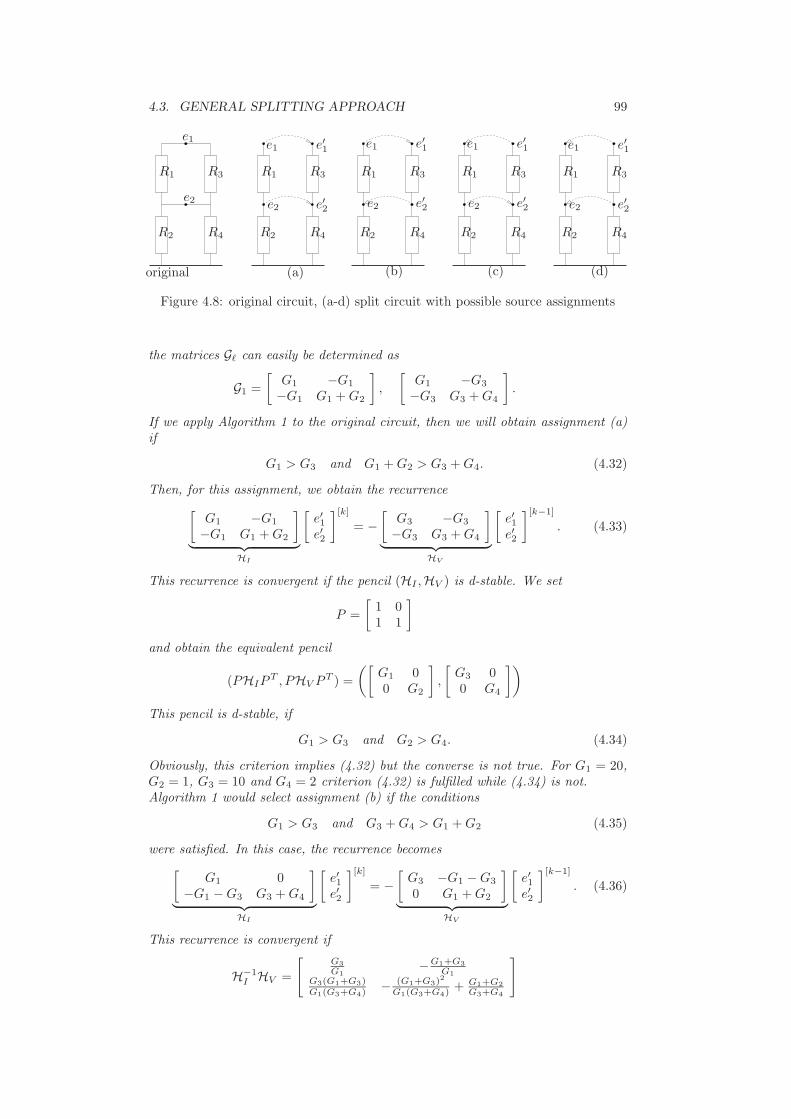
4.3. GENERAL SPLITTING APPROACH 99
original (a) (b) (c) (d)
R1 R1R1R1R1
R2 R2R2R2R2
R3 R3R3R3R3
R4 R4R4R4R4
e1 e1 e1e1e1
e2 e2 e2e2e2
e′1 e′1e′1e′1
e′2 e′2e′2e′2
Figure 4.8: original circuit, (a-d) split circuit with possible source assignments
the matrices Gℓ can easily be determined as
G1 =
[G1 −G1
−G1 G1 + G2
],
[G1 −G3
−G3 G3 + G4
].
If we apply Algorithm 1 to the original circuit, then we will obtain assignment (a)if
G1 > G3 and G1 + G2 > G3 + G4. (4.32)
Then, for this assignment, we obtain the recurrence
[G1 −G1
−G1 G1 + G2
]
︸ ︷︷ ︸HI
[e′1e′2
][k]
= −[
G3 −G3
−G3 G3 + G4
]
︸ ︷︷ ︸HV
[e′1e′2
][k−1]
. (4.33)
This recurrence is convergent if the pencil (HI ,HV ) is d-stable. We set
P =
[1 01 1
]
and obtain the equivalent pencil
(PHIPT , PHV PT ) =
([G1 00 G2
],
[G3 00 G4
])
This pencil is d-stable, if
G1 > G3 and G2 > G4. (4.34)
Obviously, this criterion implies (4.32) but the converse is not true. For G1 = 20,G2 = 1, G3 = 10 and G4 = 2 criterion (4.32) is fulfilled while (4.34) is not.Algorithm 1 would select assignment (b) if the conditions
G1 > G3 and G3 + G4 > G1 + G2 (4.35)
were satisfied. In this case, the recurrence becomes
[G1 0
−G1 − G3 G3 + G4
]
︸ ︷︷ ︸HI
[e′1e′2
][k]
= −[
G3 −G1 − G3
0 G1 + G2
]
︸ ︷︷ ︸HV
[e′1e′2
][k−1]
. (4.36)
This recurrence is convergent if
H−1I HV =
[G3
G1−G1+G3
G1
G3(G1+G3)G1(G3+G4) − (G1+G3)
2
G1(G3+G4)+ G1+G2
G3+G4
]

100 CHAPTER 4. DIM IN CIRCUIT SIMULATION
is contractive. The characteristic polynomial of H−1I HV is given by
p(λ) = λ2 − aλ + b (4.37)
with
a =G1(G2 − G3) + G3(G4 − G1)
G1(G3 + G4),
b =G3(G1 + G2)
G1(G3 + G4).
We avoid computing the roots of p directly by applying the Jury-criterion, cf. [82].This criterion gives necessary and sufficient conditions on the coefficients of a poly-nomial such that the roots all lie inside the unit disc. For the polynomial p in (4.37),these conditions are
p(0) = b < 1, (4.38a)
p(1) = 1 − a + b > 0, (4.38b)
p(−1) = 1 + a + b > 0. (4.38c)
An additional condition that arises from the nature of the example is
Gℓ > 0, ℓ = 1, . . . , 4. (4.38d)
Conditions (4.38a) and (4.38d) together yield
G3G2 < G1G4 or equivalentlyG3
G1<
G4
G2. (4.39a)
Condition (4.38b) can be transformed into
4G1G3 + (G1 − G3)(G4 − G2) > 0, (4.39b)
while Condition (4.38c) is equivalent to
(G1 + G3)(G2 + G4) > 0. (4.40)
With (4.38d), Inequality (4.40) is always true. Hence, if and only if (4.39) holdsthen H−1
I HV is contractive.It can then be seen that Criterion (4.35) implies (4.39). The same counterexampleas above (G1 = 20, G2 = 1, G3 = 10, G4 = 2) shows that the converse is nottrue. Criterion (4.39) is fulfilled, but not (4.35). Instead, assignment (a) would bechosen by Algorithm 1 which, as seen above, leads to divergence.Another example is G1 = 20, G2 = 0, G3 = 10 and G4 = 1. The value G2 = 0means that the circuit is open at that point and the resistor R1 has no connection toground in subcircuit 1. In this case, the algorithm would first choose assignment (a)in line 4 and then reject that choice in line 6 because R1 would only be connectedto ground via current sources. In can then be shown that no consistent assignmentexists such that convergence is achieved.
We have seen that it is possible that Algorithm 1 selects source assignments thatwill not lead to convergence. In other cases the selected assignment is suitable, butit is not found for all configurations of elements that would require that assignment.It is even possible that no valid assignment exists. But first, we will generalize theresults for resistive circuits to general RCL circuits.
In this section we have demonstrated how, starting from an electrical circuit with
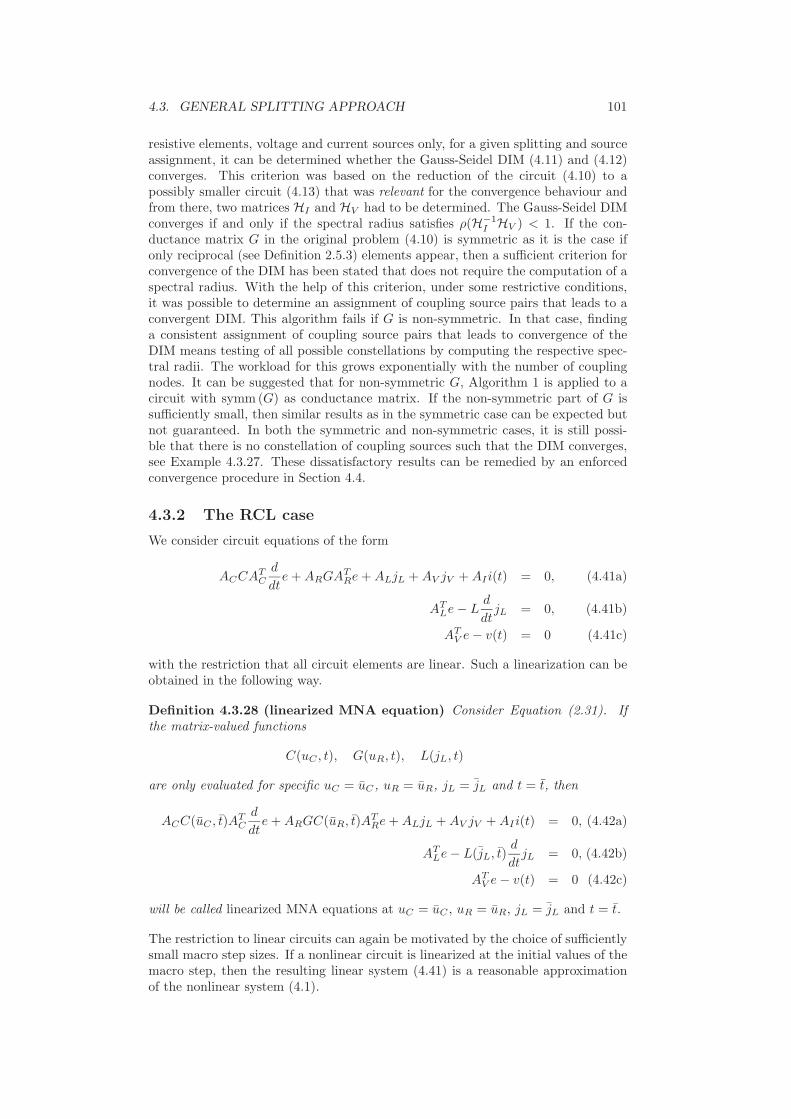
4.3. GENERAL SPLITTING APPROACH 101
resistive elements, voltage and current sources only, for a given splitting and sourceassignment, it can be determined whether the Gauss-Seidel DIM (4.11) and (4.12)converges. This criterion was based on the reduction of the circuit (4.10) to apossibly smaller circuit (4.13) that was relevant for the convergence behaviour andfrom there, two matrices HI and HV had to be determined. The Gauss-Seidel DIMconverges if and only if the spectral radius satisfies ρ(H−1
I HV ) < 1. If the con-ductance matrix G in the original problem (4.10) is symmetric as it is the case ifonly reciprocal (see Definition 2.5.3) elements appear, then a sufficient criterion forconvergence of the DIM has been stated that does not require the computation of aspectral radius. With the help of this criterion, under some restrictive conditions,it was possible to determine an assignment of coupling source pairs that leads to aconvergent DIM. This algorithm fails if G is non-symmetric. In that case, findinga consistent assignment of coupling source pairs that leads to convergence of theDIM means testing of all possible constellations by computing the respective spec-tral radii. The workload for this grows exponentially with the number of couplingnodes. It can be suggested that for non-symmetric G, Algorithm 1 is applied to acircuit with symm(G) as conductance matrix. If the non-symmetric part of G issufficiently small, then similar results as in the symmetric case can be expected butnot guaranteed. In both the symmetric and non-symmetric cases, it is still possi-ble that there is no constellation of coupling sources such that the DIM converges,see Example 4.3.27. These dissatisfactory results can be remedied by an enforcedconvergence procedure in Section 4.4.
4.3.2 The RCL case
We consider circuit equations of the form
ACCATC
d
dte + ARGAT
Re + ALjL + AV jV + AIi(t) = 0, (4.41a)
ATLe − L
d
dtjL = 0, (4.41b)
ATV e − v(t) = 0 (4.41c)
with the restriction that all circuit elements are linear. Such a linearization can beobtained in the following way.
Definition 4.3.28 (linearized MNA equation) Consider Equation (2.31). Ifthe matrix-valued functions
C(uC , t), G(uR, t), L(jL, t)
are only evaluated for specific uC = uC , uR = uR, jL = jL and t = t, then
ACC(uC , t)ATC
d
dte + ARGC(uR, t)AT
Re + ALjL + AV jV + AI i(t) = 0, (4.42a)
ATLe − L(jL, t)
d
dtjL = 0, (4.42b)
ATV e − v(t) = 0 (4.42c)
will be called linearized MNA equations at uC = uC , uR = uR, jL = jL and t = t.
The restriction to linear circuits can again be motivated by the choice of sufficientlysmall macro step sizes. If a nonlinear circuit is linearized at the initial values of themacro step, then the resulting linear system (4.41) is a reasonable approximationof the nonlinear system (4.1).

102 CHAPTER 4. DIM IN CIRCUIT SIMULATION
It is common to assume that symm C, symm G and symm L are positive definite,i.e., that the network is passive, see Definition 2.5.8.We are interested in the convergence of dynamic iteration methods for (4.41). Hence,with Observation 4.3.12, we do not need to consider independent sources in thecircuit equations. Setting v(t) = 0 and i(t) = 0 does not change the convergencebehaviour of dynamic iteration methods but simplifies the circuit. As in the caseof purely resistive circuits in Section 4.3.1, we contract the nodes of voltage sourcesand remove current sources. However, coupling sources as in Equations (4.4a) and(4.4d) will have to be included into the circuit equations. Before splitting, withoutindependent sources but with coupling sources, the considered circuit DAE is of theform
ACCATC
d
dte + ARGAT
Re + ALjL + AKjK = AKjK , (4.43a)
ATLe − L
d
dtjL = 0, (4.43b)
ATKe = AT
Ke. (4.43c)
It can easily be seen that
e = 0, jL = 0, jK = 0
is a solution. For zero initial conditions, this is also a fixed point solution in aGauss-Seidel DIM applied to (4.43). We will subsequently investigate under whichconditions, this fixed point is attractive and the DIM converges.We notice that (4.43) is a purely linear DAE. Hence, it makes sense to perform aLaplace transform 2.2.11. Let
E(s) = L (e(t)), JL(s) = L (jL(t)), JK(s) = L (jK(t))
be the transformed variables for e, jL and jK . Assuming zero initial conditions, thetransformed equations (4.43) are of the form
sACCATCE + ARGAT
RE + ALJL + AKJK = AKJK , (4.44a)
ATLE − sLJL = 0, (4.44b)
ATKE = AT
KE. (4.44c)
Inserting (4.44b) into (4.44a) yields
(sACCATC + ARGAT
R + s−1ALL−1ATL)E + AKJK = AKJK , (4.45a)
ATKE = AT
KE. (4.45b)
The structure of (4.45) bears a certain resemblance to the equations in the purelyresistive case in Section 4.3.1. The vector of transformed potentials E consistsof potentials at coupling nodes EK and potentials at the remaining nodes EK . Asbefore, we will reduce the vector of unknown potentials to EK . However, this provesto be more difficult than in the resistive case. We need to perform a splitting ofthe circuit graph, one that isolates capacitive, resistive and inductive subgraphs.We will be using the definition of subgraphs and matrices as in Section 2.5.3 andTables 2.1 and 2.2. We apply the Gauss-Seidel DIM to (4.45). The resulting MNAequations for both subsystems are of the form
(sAC1C1ATC1 + AR1G1A
TR1 + s−1AL1L
−11 AT
L1)E[k]1 + AK1J
[k]K1
= ST1 S2AK2J
[k−1]K2 , (4.46a)
ATK1E
[k]1 = AT
K1ST1 S2E
[k−1]2 . (4.46b)

4.3. GENERAL SPLITTING APPROACH 103
and
(sAC2C2ATC2 + AR2G2A
TR2 + s−1AL2L
−12 AT
L2)E[k]2 + AK2J
[k]K2
= ST2 S1AK1J
[k]K1, (4.47a)
ATK2E
[k]2 = AT
K2ST2 S1E
[k]1 (4.47b)
where S1 and S2 are selection matrices as described in Definition 4.3.10 and
Eℓ = STℓ E, A∗ℓ = ST
ℓ A∗, ∗ ∈ C, G, L, ℓ = 1, 2.
The matrices AKℓ are such that a reordering of the columns of [S1AK1, S2AK2]yields AK . Analogously S1JK1 + S2JK2 is an appropriate reordering of [S1, S2]JK .We need to restructure Equations (4.46) and (4.47). To that end we will introducethe following subcircuits.
Let G(N, B) be the graph of a pre-splitting circuit with linear constant elementsfulfilling Assumptions 4.3.1 and 4.3.9. Furthermore we assume that, after splitting,the circuit fulfills Assumption 4.3.13. As in Table 2.1, we construct the subgraphGC of G by removing all branches that are not occupied by capacitive elements.Now, every component that does not contain a coupling node is equally removedfrom GC . In the remaining components, one coupling node is chosen and identi-fied with the ground node n⊤. If the component contains n⊤ already, then it isnot changed. Any branches forming self loops are removed as well. The remaininggraph will be called GC . We construct the subgraph GG−C of G by removing allinductive branches and contracting all capacitive branches. Then, GG−C consists ofresistive branches only. In analogy to GC , components without coupling nodes areremoved altogether. In every other component, a coupling node is identified withn⊤, except if the component already contains the ground node. After the removalof possible self-loops, the remaining graph will be called GG−C . We consider thesubgraph GL−CG that is obtained from G by contracting all non-inductive branchesand removing possible self-loops. Every component without coupling nodes is re-moved. In every other component, a coupling node is identified with n⊤, except ifthe component already contains the ground node.
Definition 4.3.29 (C-, G- and L-subcircuits)
Let GC , GG−C and GL−CG be constructed as above. Then, the circuits that have
the representing graphs GC , GG−C and GL−CG will be referred to as C-subcircuit,
G-subcircuit and L-subcircuit, respectively.

104 CHAPTER 4. DIM IN CIRCUIT SIMULATION
C R1
R2
L1
L2
L3
0
1
2
3
Figure 4.9: example RCL circuit
C
0
1
R2
0
2
L3
0
3
Figure 4.10: C-, G- and L-subcircuits
Example 4.3.30 Consider the simple example circuit in Figure 4.9. Let
G(N, B) = G(0, 1, 2, 3, C, R1, R2, L1, L2, L3)
be the graph of the circuit with incidence relations as in the figure, where 0 is theground node. We assume that all other nodes are coupling nodes.We want to determine the C-, G- and L-subcircuits, respectively. Following theapproach described above, we first remove all non-capacitive branches from G. Thisleads to the three subgraphs GC1(0, 1, C), GC2(2, ∅) and GC3(3, ∅). Now,in each subgraph, one node is chosen as reference node and identified with the groundnode 0. In this way, the circuits corresponding to GC2 and GC3 vanish. The sub-graph GC1 already contains the ground node and is, thus, unchanged. The circuitrepresented by GC1 is the C subcircuit.For the construction of the G-subcircuit, we contract all capacitive branches in G.This identifies node 1 with the ground 0 and creates two self-loops of the branchesR1 and L1. These loops, as well as all remaining inductive branches are removed.This leads to two subgraphs GR2(0, 2, R2), and GR3(3, ∅). Identifying onenode in each subgraph with 0, the subcircuit defined by GR3 vanishes, while the un-changed GR2 is the graph of the R subcircuit.

4.3. GENERAL SPLITTING APPROACH 105
For the construction of the L-subcircuit, all non-inductive branches are contracted.This leads the identification of nodes 1 and 2 with 0. The arising self-loops of thebranches C, R1, R2, L1 and L2 are removed. The remaining graph is GL3(0, 3, L3)which already contains 0 and represents the L-subcircuit.The C-, G- and L-subcircuits are depicted in Figure 4.10.
Subsequently, the term C-, G- and L-subcircuit will also be employed to address theparts of a circuit that would constitute the respective subcircuits if the contractionsdescribed above were performed.The G-subcircuit is a purely resistive circuit, whereas the C- and L-subcircuits arenot. The resulting MNA equations for these three subcircuits have the form
A∗M∗AT∗ E∗ + AK∗JK∗ = AK∗JK∗, (4.48)
ATK∗E∗ = AT
K∗E∗,
where ∗ ∈ C, G, L and MC = sC, MG = G and ML = (sL)−1 are the element
matrices in the C-, G- and L-subcircuits. After splitting any of these circuits andapplying the Gauss-Seidel DIM, we obtain recurrence equations of the form
A∗1M∗1AT∗1E
[k]∗1 + AK∗1J
[k]K∗1 = ST
∗1S∗2AK∗2J[k−1]K∗2 , (4.49a)
ATK∗1E
[k]∗1 = AT
K∗1ST∗1S∗2E
[k−1]∗2 , (4.49b)
A∗2M∗2AT∗2E
[k]∗2 + AK∗2J
[k]K∗2 = ST
∗2S∗1AK∗1J[k]K∗1, (4.50a)
ATK∗2E
[k]∗2 = AT
K∗2ST∗2S∗1E
[k]∗1 . (4.50b)
Each of the systems (4.49) together with (4.50), ∗ ∈ C, G, L is of the samestructure as a purely resistive coupled circuit (4.14) and (4.15) and can be treatedby the techniques in Section 4.3.1. Convergence of each of the systems can then becharacterized by a spectral radius of the form
ρ(H−1∗I H∗V ), ∗ ∈ C, G, L.
The formal factors s and s−1 that appear in the cases ∗ ∈ C, L cancel in H−1∗I H∗V .
We will subsequently show that convergence of the DIM (4.46) with (4.47) can becharacterized by the convergence behaviour of the three systems (4.49) togetherwith (4.50), ∗ ∈ C, G, L.
Consider the matrix
UT =
II [
Y TL−CR
ZTL−CR
]
I [Y T
R−C
ZTR−C
][
Y TC
ZTC
](4.51a)
=
Y TC
Y TR−CZT
C
Y TL−CRZT
R−CZTC
ZTL−CRZT
R−CZTC
(4.51b)
=
Y TC
Y TR−CZT
C
Y TL−CRZT
CR
ZTCRL
, (4.51c)

106 CHAPTER 4. DIM IN CIRCUIT SIMULATION
with ZTCR = ZT
R−CZTC and ZT
CRL = ZTL−CRZT
CR. With Corollary 2.4.32, thecolumns of ZCRL span the image of the reduced incidence matrix of the circuitgraph after contraction of all capacitances, resistances and inductances. For cir-cuits that fulfill Assumption 4.3.1, this is only the ground node and ZT
CRL has zerocolumns and can be omitted. Thus, we may assume that ZCRL vanishes. Hence,
UT =
Y TC
Y TR−CZT
C
Y TL−CRZT
CR
.
By construction, the matrices [YC , ZC ], [YR−C , ZR−C ] and [YL−CR, ZL−CR] are allnonsingular. Thus, with the construction (4.51) of UT , the matrix U is nonsingularand we can multiply (4.44a) by UT . Furthermore, we perform a change of variables
E = U
EC
ER−C
EL−CR
.
Here, EC are voltages in the C-subcircuit, ER−C are voltages in the G-subcircuit,
and EL−CR are voltages in the L-subcircuit. These voltages are always the difference
of a potential of a node in a component in the C-, G- or L-subcircuit and thereference node in that component. In this way, EC , ER−C and EL−CR can be seenas generalized potentials.Additionally, we assume that EC , ER−C and EL−CR are ordered in such a way thatthe leading entries in the vector are the generalized potentials of the splitting nodesfollowed by the generalized potentials at non-splitting nodes. For example,
EC =
[EKC
EKC
],
where EKC are voltages from splitting nodes and EKC are voltages from non-splitting nodes to the respective reference node. Such an ordering is always possible,since it only depends on the ordering of the columns of YC = [YCK , YCK ]. Afterthese transformations, (4.44a) becomes
UT (sACCATC + ARGAT
R + s−1ALL−1ATL)U
EKC
EKC
EKR−C
EKR−C
EKL−CR
EKL−CR
+ UT AKJK
= UT AKJK , (4.52)
ATKU
EKC
EKC
EKR−C
EKR−C
EKL−CR
EKL−CR
= ATKU
EKC
EKC
EKR−C
EKR−C
EKL−CR
EKL−CR
.(4.53)
The aim of the following subsections will be to develop the DIM equations for theC-, G- and L-subcircuits and to establish explicit recurrence equations from oneiteration step to the next, similar to (4.30) for the purely resistive case. Many ofthe techniques that were used to construct (4.30) will also be applied to that aim.Then, we will interpret the findings in the context of the whole coupled system ofcircuits (4.46) and (4.47).

4.3. GENERAL SPLITTING APPROACH 107
4.3.2.1 The C-subcircuit
With Y TC AC = AC and ZT
CAC = 0, we have
UT ACCATCU =
ACCATC
00
,
where
ACCATC =
[ACK
ACK
]C
[ACK
ACK
]T
def=
[CKK CKK
CKK CKK
].
The matrix YC as defined in Section 2.5.3 consists of unit vectors only. The sameapplies to AK . Hence, the product Y T
C AK has entries 0 or 1, with at most one1 in every row and column. More specifically, with YC = [YCK YCK ], we haveY T
CKAK = 0 as the 1 in every column of YCK is in the position of a non-splitting
node and in the columns of AK it is only in the position of splitting nodes. Asthese nodes never coincide, the scalar product always vanishes. With a similarargument, it can be shown that with a proper ordering of the columns of AK , we
have Y TC AK =
[I0
]. This is the incidence matrix of the coupling sources with
respect to the C-subcircuit. We will define Y TC AKJK as JKC . Thus, the part of
(4.52) together with (4.53) that refers to the C-subcircuit is
s
[CKK CKK
CKK CKK
] [EKC
EKC
]+ O(1)
EKC
EKC
ER−C
EL−CR
+
[I0
]JKC =
[I0
]JKC , (4.54a)
EKC =EKC . (4.54b)
The O(·) notation is used to illustrate, that the only terms with the factor s inthem are the potentials EKC and EKC . Also, for a shorter notation, the voltagesER−C and EL−CR are not noted in their split representations.
We will initially only consider the C-subcircuit where all resistive and inductivebranches, as well as all non-relevant capacitive branches are removed. In thatcase, ER−C and EL−CR disappear from the KCL part of the MNA equations.The voltages EKC and EKC represent differences between node potentials, i.e.,every node potential of a component of the C-subgraph and a unique referencenode for each such component. By design, the reference nodes are always splittingnodes. As these nodes are duplicated in the splitting process, both subcircuits havecorresponding reference nodes and all generalized potentials are well defined aftersplitting. Moreover, in the C-subcircuit, all nodes not incident with capacitors areset to ground as are the reference nodes in every component. The resulting circuitconsists of capacitances and coupling sources only and every node is connected tothe ground via a path along capacitive branches only. The resulting MNA equationscan be obtained from (4.54) by dropping the O(1) terms.
s
[CKK CKK
CKK CKK
] [EKC
EKC
]+
[I0
]JKC =
[I0
]JKC , (4.55a)
EKC = EKC . (4.55b)
This equation is of the form (4.48). In order to construct the DIM equations from(4.55), we define selection matrices SCℓ, ℓ = 1, 2 via
STCℓEC =
[EKCℓ
EKCℓ
].

108 CHAPTER 4. DIM IN CIRCUIT SIMULATION
We now obtain a set of equations as in (4.49) and (4.50) as the DIM equations
s
[CKK1 CKK1
CKK1 CKK1
] [EKC1
EKC1
][k]
+ AKC1J[k]KC1 = ST
C1SC2AKC2J[k−1]KC2 ,
ATKC1E
[k]KC1 = AT
KC1STC1SC2E
[k−1]KC2 ,
s
[CKK2 CKK2
CKK2 CKK2
] [EKC2
EKC2
][k]
+ AKC2J[k]KC2 = ST
C2SC1AKC1J[k]KC1,
ATKC2E
[k]KC2 = AT
KC2STC2SC1E
[k]KC1.
We additionally assume that EKCℓ is ordered as
[EKCV ℓ
EKCIℓ
]just as eK was split in
the resistive case (4.16). Then STC1SC2 has the structure
STC1SC2 =
0 InCKV 10
InCKV 20 0
0 0 0
,
where nCKV ℓ is the number of coupling voltage sources in each C-subcircuit. Inthis form, the equations for the first subsystem become
sCKK1
[EKCV 1
EKCI1
][k]
+ sCKK1E[k]
KC1+
[J
[k]KC1
0
]=
[0
J[k−1]KC2
], (4.56a)
sCKK1
[EKCV 1
EKCI1
][k]
+ sCKK1E[k]
KC1= 0, (4.56b)
E[k]KCV 1 = E
[k−1]KCI2. (4.56c)
Equation (4.56b) is KCL applied to all relevant non-coupling nodes of the C-subcircuit of circuit 1. With the definition of relevant branches, Definition 4.3.16,the currents through relevant branches. As there are no non-coupling sources in(4.56), this implies that the generalized potentials at relevant non-coupling nodesare uniquely defined by the potentials of coupling nodes. Hence, the matrix CKK
is invertible and we can substitute
E[k]
KC1= −C−1
KK1CKK1
[EKCV 1
EKCI1
][k]
in (4.56). With
C1 = CKK1 − CKK1C−1KK1
CKK1,
we obtain
C1
[EKCV 1
EKCI1
][k]
+
[J
[k]KC1
0
]=
[0
J[k−1]KC2
], (4.57a)
E[k]KCV 1 = E
[k−1]KCI2. (4.57b)
Similarly, we obtain the equations for the second subsystem as
C2
[EKCV 2
EKCI2
][k]
+
[J
[k]KC2
0
]=
[0
J[k]KC1
], (4.58a)
E[k]KCV 2 = E
[k]KCI1, (4.58b)

4.3. GENERAL SPLITTING APPROACH 109
where
C2 = CKK2 − CKK2C−1KK2
CKK .
Proceeding analogously as in the purely resistive case, with the splitting
Cℓ =
[CV V ℓ CV Iℓ
CIV ℓ CIIℓ
], ℓ = 1, 2,
we define
HCI =
[CII1 0
CV I1 + CIV 2 CII2
], HCV =
[CV V 2 CV I2 + CIV 1
0 CV V 1
].
In this way, we arrive at an analogous result to Theorem 4.3.21. For the recurrence
sHCI
[EKCV 2
EKCI2
][k]
= −sHCV
[EKCV 2
EKCI2
][k−1]
or after dividing by s,
HCI
[EKCV 2
EKCI2
][k]
= −HCV
[EKCV 2
EKCI2
][k−1]
,
convergence depends on whether γC < 1 with γC = ρ(H−1CIHCV ). The nonsingu-
larity of HCI can usually be assumed as it was done in the resistive case. Thiswhole approach did not take into account that in (4.54) some O(1) terms appear.All steps can be performed analogously until (4.56) but then the O(1) terms pre-vent the substitution of EKCK1
. However, a sufficiency result can be achieved aspresented in the following lemma.
Lemma 4.3.31Consider the DIM system given by
sCKK1
[EKCV 1
EKCI1
][k]
+ sCKK1E[k]
K1C+ O(1)
EKC1
EKC1
ER−C1
EL−CR1
[k]
+
[J
[k]KC1
0
](4.59a)
=
[0
J[k−1]KC2
],
sCKK1
[EKCV 1
EKCI1
][k]
+ sCKK1E[k]
KC1+ O(1)
EKC1
EKC1
ER−C1
EL−CR1
[k]
= 0, (4.59b)
E[k]KCV 1 = E
[k−1]KCI2 (4.59c)
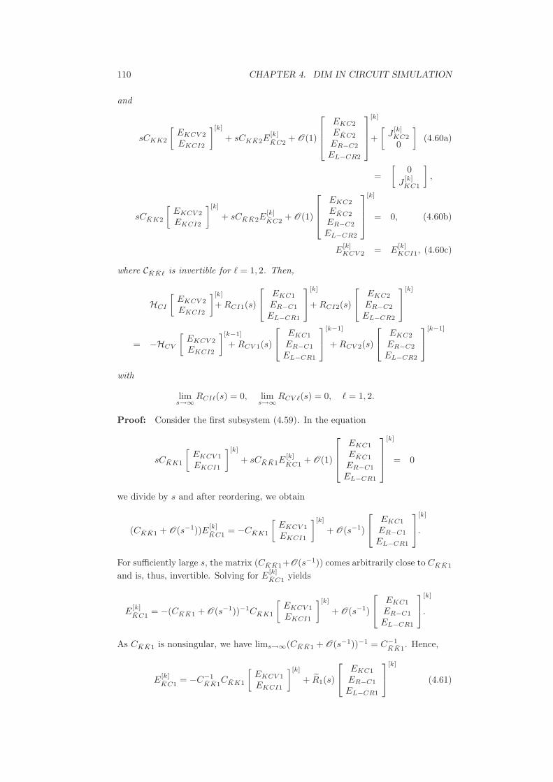
110 CHAPTER 4. DIM IN CIRCUIT SIMULATION
and
sCKK2
[EKCV 2
EKCI2
][k]
+ sCKK2E[k]
KC2+ O(1)
EKC2
EKC2
ER−C2
EL−CR2
[k]
+
[J
[k]KC2
0
](4.60a)
=
[0
J[k]KC1
],
sCKK2
[EKCV 2
EKCI2
][k]
+ sCKK2E[k]
KC2+ O(1)
EKC2
EKC2
ER−C2
EL−CR2
[k]
= 0, (4.60b)
E[k]KCV 2 = E
[k]KCI1, (4.60c)
where CKKℓ is invertible for ℓ = 1, 2. Then,
HCI
[EKCV 2
EKCI2
][k]
+ RCI1(s)
EKC1
ER−C1
EL−CR1
[k]
+ RCI2(s)
EKC2
ER−C2
EL−CR2
[k]
= −HCV
[EKCV 2
EKCI2
][k−1]
+ RCV 1(s)
EKC1
ER−C1
EL−CR1
[k−1]
+ RCV 2(s)
EKC2
ER−C2
EL−CR2
[k−1]
with
lims→∞
RCIℓ(s) = 0, lims→∞
RCV ℓ(s) = 0, ℓ = 1, 2.
Proof: Consider the first subsystem (4.59). In the equation
sCKK1
[EKCV 1
EKCI1
][k]
+ sCKK1E[k]
KC1+ O(1)
EKC1
EKC1
ER−C1
EL−CR1
[k]
= 0
we divide by s and after reordering, we obtain
(CKK1 + O(s−1))E[k]
KC1= −CKK1
[EKCV 1
EKCI1
][k]
+ O(s−1)
EKC1
ER−C1
EL−CR1
[k]
.
For sufficiently large s, the matrix (CKK1+O(s−1)) comes arbitrarily close to CKK1
and is, thus, invertible. Solving for E[k]
KC1yields
E[k]
KC1= −(CKK1 + O(s−1))−1CKK1
[EKCV 1
EKCI1
][k]
+ O(s−1)
EKC1
ER−C1
EL−CR1
[k]
.
As CKK1 is nonsingular, we have lims→∞(CKK1 + O(s−1))−1 = C−1KK1
. Hence,
E[k]
KC1= −C−1
KK1CKK1
[EKCV 1
EKCI1
][k]
+ R1(s)
EKC1
ER−C1
EL−CR1
[k]
(4.61)

4.3. GENERAL SPLITTING APPROACH 111
for an appropriate R1 with lims→∞ R1(s) = 0. We insert (4.61) into (4.59) andobtain
sC1
[EKCV 1
EKCI1
][k]
+ sR′1(s)
EKC1
ER−C1
EL−CR1
[k]
+
[J
[k]KC1
0
]=
[0
J[k−1]KC2
],
E[k]KCV 1 = E
[k−1]KCI2
with appropriate R′1(s) and lims→∞ R′
1(s) = 0. Analogously, for the second system(4.59) we obtain
sC2
[EKCV 2
EKCI2
][k]
+ sR′2(s)
EKC2
ER−C2
EL−CR2
[k]
+
[J
[k]KC1
0
]=
[0
J[k]KC1
],
E[k]KCV 2 = E
[k]KCI1
with R′2(s) such that lims→∞ R′
2(s) = 0. Following the same steps as for (4.57) and(4.58), we obtain the assertion.
4.3.2.2 The G-subcircuit
By definition Y TR−CZT
CAR = AR and ZTCRAR = 0. Hence, we have
UT ARGATRU =
Y TC ARGAT
RYC Y TC ARGAT
R 0
ARGATRYC ARGAT
R 00 0 0
,
where
ARGATR =
[ARK
ARK
]G
[ARK
ARK
]T
def=
[GKK GKK
GKK GKK
].
We investigate the MNA equations for the G-subcircuit:
ARGATRYCEC +
[GKK GKK
GKK GKK
] [EKR−C
EKR−C
]
+O(s−1)
EC
EKR−C
EKR−C
EL−CR
+ Y T
R−CZTCAKJK = Y T
R−CZTCAKJK , .(4.62a)
The equations for the coupling voltage sources are
ATKU
EC
EKR−C
EKR−C
EL−CR
= AT
KU
EC
EKR−C
EKR−C
EL−CR
. (4.62b)
In contrast to the C-subcircuit, the term for the coupling currents Y TR−CZT
CAKJK
not only selects the currents through coupling sources incident with coupling nodesin the G-circuit but also with the C-circuit. This can be explained by the waythese subcircuits are constructed. As the G-circuit is obtained after contracting
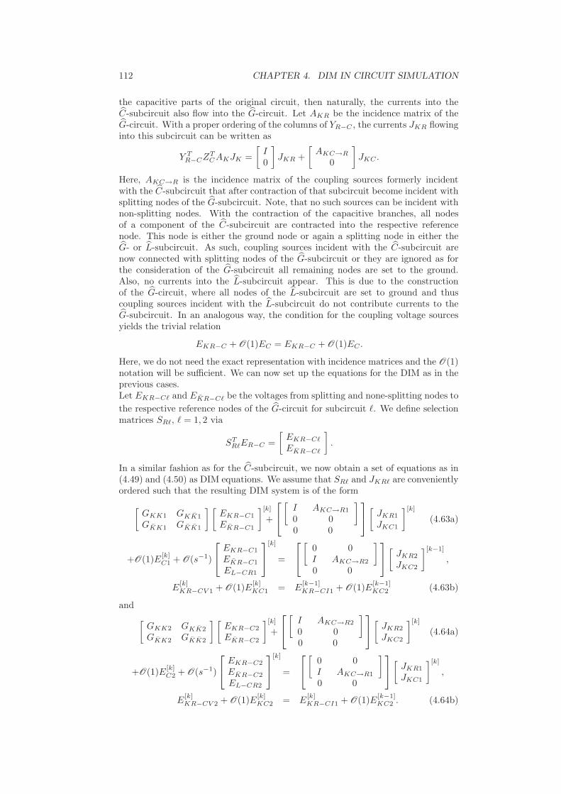
112 CHAPTER 4. DIM IN CIRCUIT SIMULATION
the capacitive parts of the original circuit, then naturally, the currents into theC-subcircuit also flow into the G-circuit. Let AKR be the incidence matrix of theG-circuit. With a proper ordering of the columns of YR−C , the currents JKR flowinginto this subcircuit can be written as
Y TR−CZT
CAKJK =
[I0
]JKR +
[AKC→R
0
]JKC .
Here, AKC→R is the incidence matrix of the coupling sources formerly incidentwith the C-subcircuit that after contraction of that subcircuit become incident withsplitting nodes of the G-subcircuit. Note, that no such sources can be incident withnon-splitting nodes. With the contraction of the capacitive branches, all nodesof a component of the C-subcircuit are contracted into the respective referencenode. This node is either the ground node or again a splitting node in either theG- or L-subcircuit. As such, coupling sources incident with the C-subcircuit arenow connected with splitting nodes of the G-subcircuit or they are ignored as forthe consideration of the G-subcircuit all remaining nodes are set to the ground.Also, no currents into the L-subcircuit appear. This is due to the constructionof the G-circuit, where all nodes of the L-subcircuit are set to ground and thuscoupling sources incident with the L-subcircuit do not contribute currents to theG-subcircuit. In an analogous way, the condition for the coupling voltage sourcesyields the trivial relation
EKR−C + O(1)EC = EKR−C + O(1)EC .
Here, we do not need the exact representation with incidence matrices and the O(1)notation will be sufficient. We can now set up the equations for the DIM as in theprevious cases.Let EKR−Cℓ and EKR−Cℓ be the voltages from splitting and none-splitting nodes to
the respective reference nodes of the G-circuit for subcircuit ℓ. We define selectionmatrices SRℓ, ℓ = 1, 2 via
STRℓER−C =
[EKR−Cℓ
EKR−Cℓ
].
In a similar fashion as for the C-subcircuit, we now obtain a set of equations as in(4.49) and (4.50) as DIM equations. We assume that SRℓ and JKRℓ are convenientlyordered such that the resulting DIM system is of the form
[GKK1 GKK1
GKK1 GKK1
] [EKR−C1
EKR−C1
][k]
+
[
I0
AKC→R1
0
]
0 0
[
JKR1
JKC1
][k]
(4.63a)
+O(1)E[k]C1 + O(s−1)
EKR−C1
EKR−C1
EL−CR1
[k]
=
[
0I
0AKC→R2
]
0 0
[
JKR2
JKC2
][k−1]
,
E[k]KR−CV 1 + O(1)E
[k]KC1 = E
[k−1]KR−CI1 + O(1)E
[k−1]KC2 (4.63b)
and
[GKK2 GKK2
GKK2 GKK2
] [EKR−C2
EKR−C2
][k]
+
[
I0
AKC→R2
0
]
0 0
[
JKR2
JKC2
][k]
(4.64a)
+O(1)E[k]C2 + O(s−1)
EKR−C2
EKR−C2
EL−CR2
[k]
=
[
0I
0AKC→R1
]
0 0
[
JKR1
JKC1
][k]
,
E[k]KR−CV 2 + O(1)E
[k]KC2 = E
[k]KR−CI1 + O(1)E
[k−1]KC2 . (4.64b)

4.3. GENERAL SPLITTING APPROACH 113
In these equations, the voltages EKR−Cℓ have been split into
[EKR−CV ℓ
EKR−CIℓ
], ℓ =
1, 2, and the KCL equations have been ordered likewise, according to whether acoupling voltage source or current source enters the respective node.As in the previous cases, we eliminate the voltages at non-splitting nodes and replacethe coupling currents JKR and JKC in order to obtain a recurrence for EKR−C2.
Lemma 4.3.32Consider the DIM system (4.63) and (4.64). Then,
HGI
[EKR−CV 2
EKR−CI2
][k]
+ O(1)E[k]C1 + O(1)E
[k]C2
+RR−CI1(s)
[EKR−C1
EL−CR1
][k]
+ RR−CI2(s)
[EKR−C1
EL−CR1
][k]
= −HGV
[EKR−CV 2
EKR−CI2
][k−1]
+ O(1)E[k−1]C1 + O(1)E
[k−1]C2
+RR−CV 1(s)
[EKR−C1
EL−CR1
][k−1]
+ RR−CV 2(s)
[EKR−C2
EL−CR2
][k−1]
with
lims→∞
RR−CIℓ(s) = 0, lims→∞
RR−CV ℓ(s) = 0, ℓ = 1, 2.
The matrices HGI and HGV are defined as
HGI =
[GII1 0
GV I1 + GIV 2 GII2
], HGV =
[GV V 2 GV I2 + GIV 1
0 GV V 1
],
with
GKKℓ − GKKℓG−1KKℓ
GKKℓ = Gℓ =
[GV V ℓ GV Iℓ
GIV ℓ GIIℓ
], ℓ = 1, 2
and where GKKℓ, ℓ = 1, 2, are invertible.
Proof: Consider only the first system (4.63). In the KCL equations for thenon-splitting nodes, we have
GKK1E[k]KR−C1 + GKK1E
[k]
KR−C1+ O(1)E
[k]C1 + O(s−1)
EKR−C1
EKR−C1
EL−CR1
[k]
= 0.
We apply the same technique as in the proof of Lemma 4.3.31. As in the case of the
C-subcircuit, we can deduce that GKK1 is nonsingular and we solve for E[k]
KR−C1
E[k]
KR−C1= G−1
KK1GKK1E
[k]KR−C1 + O(1)E
[k]C1 + R1(s)
[EKR−C1
EL−CR1
][k]
(4.65)
with a suitable R1 such that lims→∞ R1(s) = 0. We insert this expression for
E[k]
KR−C1into the KCL equations belonging to splitting nodes in (4.63a) to obtain
[GV V 1 GV I1
GIV 1 GII1
] [EKR−CV 1
EKR−CI1
][k]
+
[I AKC→R1
0 0
] [JKR1
JKC1
][k]
+O(1)E[k]C1 + O(s−1)
[EKR−C1
EL−CR1
][k]
=
[0 0I AKC→R2
] [JKR2
JKC2
][k−1]
.

114 CHAPTER 4. DIM IN CIRCUIT SIMULATION
For the second system (4.63), this approach yields
[GV V 2 GV I2
GIV 2 GII2
] [EKR−CV 2
EKR−CI2
][k]
+
[I AKC→R2
0 0
] [JKR2
JKC2
][k]
+O(1)E[k]C2 + O(s−1)
[EKR−C2
EL−CR2
][k]
=
[0 0I AKC→R1
] [JKR1
JKC1
][k]
.
Note that the controlling currents[
I AKC→Rℓ
] [ JKRℓ
JKCℓ
]always appear in this
form. We use (4.63b) and (4.63b) and apply the same replacement strategy as inthe purely resistive case to obtain
[GII1 0
GV I1 + GIV 2 GII2
] [EKR−CV 2
EKR−CI2
][k]
+ O(1)E[k]C1 + O(1)E
[k]C2
+RR−CI1(s)
[EKR−C1
EL−CR1
][k]
+ RR−CI2(s)
[EKR−C1
EL−CR1
][k]
= −[GV V 2 GV I2 + GIV 1
0 GV V 1
] [EKR−CV 2
EKR−CI2
][k−1]
+ O(1)E[k−1]C1 + O(1)E
[k−1]C2
+RR−CV 1(s)
[EKR−C1
EL−CR1
][k−1]
+ RR−CV 2(s)
[EKR−C2
EL−CR2
][k−1]
which is the assertion.
4.3.2.3 The L-subcircuit
The treatment of the equations of the L-subcircuit bears only minor changes com-pared to the G-subcircuit. We have Y T
L−CRZTCRAL = AL. Hence,
UT ALL−1ATLU
=
Y TC ALL−1AT
LYC Y TC ALL−1AT
LZCYR−C Y TC ALL−1AT
L
Y TR−CZT
CALL−1ATLYC Y T
R−CZTCALL−1AT
LZCYR−C Y TR−CZT
CALL−1ATL
ALL−1ATLYC ALL−1AT
LZCYR−C ALL−1ATL
and we set
ALL−1ATL =
[ALK
ALK
]L−1
[ALK
ALK
]T
def=
[LKK LKK
LKK LKK
].
Note, that L is an inductance matrix, measured in Henry (H), while in this notationLKK , LKK , etc are inverse inductances measured in 1
H. The MNA equations for
the L-subcircuit are
s−1ALL−1ATLYCEC + s−1ALL−1ZCYR−CER−C
+s−1
[LKK LKK
LKK LKK
] [EKL−CR
EKL−CR
]+ Y T
L−CRZTCRAKJK
= Y TL−CRZT
CRAKJK .
In contrast to the C- and G-subcircuits, no O(·) terms of lower order than s−1
appear anymore. We will subsequently collect the EC and ER−C summands in

4.3. GENERAL SPLITTING APPROACH 115
O(s−1)
[EC
ER−C
].
Similar to the G case, the currents flowing into the L subcircuit are composed of thecurrents through coupling sources directly incident with branches belonging to theL-subcircuit of the original circuit and the currents through sources that becomeincident with the L-subcircuit after the contraction of the C- and G-subcircuits.Hence, with proper orderings we can write
Y TL−CRZT
CRAKJK =
[I0
]JKL +
[AKC→L
0
]JKC +
[AKR→L
0
]JKR.
Similarly, the voltages across coupling voltage sources are
ATKZCRYL−CRE = EKL−CR + O(1)
[EC
ER−C
].
We proceed in the same way as in the previous subsections and with proper order-ings, we obtain the DIM equations for the split L-subcircuit as
s−1
[LKK1 LKK1
LKK1 LKK1
][EKL−CR1
EKL−CR1
][k]
+
[
I0
AKC→L1
0AKR→L1
0
]
0 0 0
JKL1
JKR1
JKC1
[k]
+O(s−1)
[EC1
ER−C1
][k]
=
[
0I
0AKC→L2
0AKR→L2
]
0 0 0
JKL2
JKR2
JKC2
[k−1]
, (4.66a)
E[k]KL−CRV 1 + O(1)
[EC1
ER−C1
][k]
= E[k−1]KL−CRI2 + O(1)
[EC2
ER−C2
][k−1]
(4.66b)
and
s−1
[LKK2 LKK2
LKK2 LKK2
][EKL−CR2
EKL−CR2
][k]
+
[
I0
AKC→L2
0AKR→L2
0
]
0 0 0
JKL2
JKR2
JKC2
[k]
+O(s−1)
[EC2
ER−C2
][k]
=
[
0I
0AKC→L1
0AKR→L1
]
0 0 0
JKL1
JKR1
JKC1
[k]
, (4.67a)
E[k]KL−CRV 2 + O(1)
[EC2
ER−C2
][k]
= E[k]KL−CRI1 + O(1)
[EC1
ER−C1
][k]
(4.67b)
Again, the voltages EKL−CRℓ have been split into
[EKL−CRV ℓ
EKL−CRIℓ
], ℓ = 1, 2, and the
KCL equations have been ordered likewise, according to whether a coupling voltagesource or current source enters the respective node.The recurrence from one iteration step to the next is given in the following lemma.
Lemma 4.3.33Consider the DIM system (4.66) and (4.67). Then,
HLI
[EKL−CRV 2
EKL−CRI2
][k]
+ O(1)
[EC1
ER−C1
][k]
+ O(1)
[EC2
ER−C2
][k]
= −HLV
[EKL−CRV 2
EKL−CRI2
][k−1]
+ O(1)
[EC1
ER−C1
][k−1]
+ O(1)
[EC2
ER−C2
][k−1]
.

116 CHAPTER 4. DIM IN CIRCUIT SIMULATION
The matrices HLI and HLV are defined as
HLI =
[LII1 0
LV I1 + LIV 2 LII2
], HLV =
[LV V 2 LV I2 + LIV 1
0 LV V 1
],
with
LKKℓ − LKKℓL−1KKℓ
LKKℓ = Lℓ =
[LV V ℓ LV Iℓ
LIV ℓ LIIℓ
], ℓ = 1, 2
and where LKKℓ, ℓ = 1, 2 are invertible.
Proof: Consider the first system (4.66). In the KCL equations for the non-splittingnodes, we have
s−1LKK1E[k]KL−CR1 + s−1LKK1E
[k]
KL−CR1+ O(s−1)
[EC1
ER−C1
][k]
= 0.
As in the previous cases, we have that LKK1 is nonsingular and we solve for
E[k]
KL−CR1
E[k]
KL−CR1= L−1
KK1LKK1E
[k]KL−CR1 + O(1)
[EC1
ER−C1
][k]
. (4.68)
We insert this expression for E[k]
KL−CR1into the KCL equations belonging to split-
ting nodes in (4.63a) to obtain
[LV V 1 LV I1
LIV 1 LII1
] [EKL−CRV 1
EKL−CRI1
][k]
+
[I AKC→L1 AKR→L1
0 0 0
]
JKL1
JKC1
JKR1
[k]
+O(1)
[EC1
ER−C1
][k]
=
[0 0 0I AKC→L2 AKR→L2
]
JKL2
JKC2
JKR2
[k−1]
.
For the second system (4.67), this approach yields
[LV V 2 LV I2
LIV 2 LII2
] [EKL−CRV 2
EKL−CRI2
][k]
+
[I AKC→L2 AKR→L2
0 0 0
]
JKL2
JKC2
JKR2
[k]
+O(1)
[EC2
ER−C2
][k]
=
[0 0 0I AKC→L1 AKR→L1
]
JKL1
JKC1
JKR1
[k]
.
We use (4.66b) and (4.67b) and apply the same replacement strategy as in theprevious cases to obtain
[LII1 0
LV I1 + LIV 2 LII2
][EKL−CRV 2
EKL−CRI2
][k]
+O(1)
[EC1
ER−C1
][k]
+O(1)
[EC2
ER−C2
][k]
= −[LV V 2 LV I2 + LIV 1
0 LV V 1
][EKL−CRV 2
EKL−CRI2
][k−1]
+O(1)
[EC1
ER−C1
][k−1]
+O(1)
[EC2
ER−C2
][k−1]
which is the assertion.
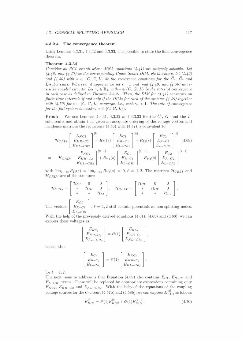
4.3. GENERAL SPLITTING APPROACH 117
4.3.2.4 The convergence theorem
Using Lemmas 4.3.31, 4.3.32 and 4.3.33, it is possible to state the final convergencetheorem.
Theorem 4.3.34Consider an RCL circuit whose MNA equations (4.41) are uniquely solvable. Let(4.46) and (4.47) be the corresponding Gauss-Seidel DIM. Furthermore, let (4.49)
and (4.50) with ∗ ∈ C, G, L be the recurrence equations for the C-, G- and
L-subcircuits. Wherever it appears, we set s = 1 and treat (4.49) and (4.50) as re-sistive coupled circuits. Let γ∗ ∈ R+ with ∗ ∈ C, G, L be the rates of convergencein each case as defined in Theorem 4.3.21. Then, the DIM for (4.41) converges onfinite time intervals if and only if the DIMs for each of the systems (4.49) togetherwith (4.50) for ∗ ∈ C, G, L converge, i.e., each γ∗ < 1. The rate of convergencefor the full system is max(γ∗, ∗ ∈ C, G, L).
Proof: We use Lemmas 4.3.31, 4.3.32 and 4.3.33 for the C-, G- and the L-subcircuits and obtain that given an adequate ordering of the voltage vectors andincidence matrices the recurrence (4.46) with (4.47) is equivalent to
HCRLI
EKC2
EKR−C2
EKL−CR2
[k]
+ RI1(s)
EC1
ER−C1
EL−CR1
[k]
+ RI2(s)
EC2
ER−C2
EL−CR2
[k]
(4.69)
= −HCRLV
EKC2
EKR−C2
EKL−CR2
[k−1]
+ RV 1(s)
EC1
ER−C1
EL−CR1
[k−1]
+ RV 2(s)
EC2
ER−C2
EL−CR2
[k−1]
with lims→∞ RIℓ(s) = lims→∞ RV ℓ(s) = 0, ℓ = 1, 2. The matrices HCRLI andHCRLV are of the structure
HCRLI =
HCI 0 0∗ HGI 0∗ ∗ HLI
, HCRLV =
HCV 0 0∗ HGV 0∗ ∗ HLV
.
The vectors
ECℓ
ER−Cℓ
EL−CRℓ
, ℓ = 1, 2 still contain potentials at non-splitting nodes.
With the help of the previously derived equations (4.61), (4.65) and (4.68), we canexpress these voltages as
EKCℓ
EKR−Cℓ
EKL−CRℓ
= O(1)
EKCℓ
EKR−Cℓ
EKL−CRℓ
,
hence, also
ECℓ
ER−Cℓ
EL−CRℓ
= O(1)
EKCℓ
EKR−Cℓ
EKL−CRℓ
,
for ℓ = 1, 2.The next issue to address is that Equation (4.69) also contains EC1, ER−C1 andEL−CR1 terms. These will be replaced by appropriate expressions containing onlyEKC2, EKR−C2 and EKL−CR2. With the help of the equations of the coupling
voltage sources for the C-circuit (4.57b) and (4.58b), we can express E[k]KC1 as follows
E[k]KC1 = O(1)E
[k]KC2 + O(1)E
[k−1]KC2 . (4.70)

118 CHAPTER 4. DIM IN CIRCUIT SIMULATION
In the same manner we have
E[k−1]KC1 = O(1)E
[k−1]KC2 + O(1)E
[k−2]KC2 . (4.71)
This approach can be repeated for E[k]KR−C1 and E
[k−1]KR−C1. Using (4.63b) and (4.64b)
we first write E[k]KR−C1 as
E[k]KR−C1 = O(1)E
[k]KR−C2 + O(1)E
[k−1]KR−C2
+O(1)E[k]KC1 + O(1)E
[k−1]KC1 + O(1)E
[k]KC2 + O(1)E
[k−1]KC2 .
The EKC1 iterates can be replaced using (4.70) and (4.71) to yield
E[k]KR−C1 = O(1)E
[k]KR−C2 + O(1)E
[k−1]KR−C2
+O(1)E[k]KC2 + O(1)E
[k−1]KC2 + O(1)E
[k−2]KC2 . (4.72)
With a shift of the iteration index, we obtain
E[k−1]KR−C1 = O(1)E
[k−1]KR−C2 + O(1)E
[k−2]KR−C2
+O(1)E[k−1]KC2 + O(1)E
[k−2]KC2 + O(1)E
[k−3]KC2 . (4.73)
For the L-subcircuit, we first use (4.66b) and (4.67b) to obtain
E[k]KL−CR1 = O(1)E
[k]KL−CR2 + O(1)E
[k−1]KL−CR2
+O(1)E[k]KC1 + O(1)E
[k−1]KC1 + O(1)E
[k]KC2 + O(1)E
[k−1]KC2
+O(1)E[k]KR−C1 + O(1)E
[k−1]KR−C1 + O(1)E
[k]KR−C2 + O(1)E
[k−1]KR−C2.
Now, using (4.70)-(4.73), the remaining EKC1 and EKR−C1 terms are replaced
E[k]KL−CR1 = O(1)E
[k]KL−CR2 + O(1)E
[k−1]KL−CR2
+O(1)E[k]KC2 + O(1)E
[k−1]KC2 + O(1)E
[k−2]KC2 (4.74)
+O(1)E[k]KR−C2 + O(1)E
[k−1]KR−C2 + O(1)E
[k−2]KR−C2 + O(1)E
[k−3]KR−C2.
With shifted iteration index, we obtain
E[k−1]KL−CR1 = O(1)E
[k−1]KL−CR2 + O(1)E
[k−2]KL−CR2
+O(1)E[k−1]KC2 + O(1)E
[k−2]KC2 + O(1)E
[k−3]KC2 (4.75)
+O(1)E[k−1]KR−C2 + O(1)E
[k−2]KR−C2 + O(1)E
[k−3]KR−C2 + O(1)E
[k−4]KR−C2.
If we insert (4.70)-(4.75) into (4.69), we obtain a recurrence equation only in EKC2,EKR−C2 and EKL−CR2 variables. However, it would be a 5-term recurrence withthe kth iterate depending on iterates k−4 to k−1. A quick consideration will showthat the appearance of iterates k − 4 to k − 2 is just an artifact arising from theambiguity of the used O(·) expressions. Consider the recurrence defined by (4.46)and (4.47). For arbitrary but fixed s, this system behaves like a purely resistivecoupled circuit. In that case we already have shown that the recurrence (4.30) fromiterate k − 1 to k exists. The kth iterate is uniquely defined if the matrix HI isnonsingular. Hence, also for a variable s as in (4.69), there must be a two-termrecurrence relating the kth iterate to the (k − 1)st.Thus, the system (4.69) can be transformed into
HCRLI
EKC2
EKR−C2
EKL−CR2
[k]
+ RI(s)
EKC2
EKR−C2
EKL−CR2
[k]
(4.76)
= −HCRLV
EKC2
EKR−C2
EKL−CR2
[k−1]
+ RV (s)
EKC2
EKR−C2
EKL−CR2
[k−1]

4.3. GENERAL SPLITTING APPROACH 119
with lims→∞ RI(s) = lims→∞ RV (s) = 0. Due to its block-lower triangular struc-ture, the matrix HCRLI is invertible if and only if the diagonal blocks HCI , HGI
and HLI are invertible. We have assumed a consistent source assignment. Hence,as in Theorem 4.3.21, the nonsingularity of HCI , HGI and HLI can be assumedand Equation (4.76) transforms to
EKC2
EKR−C2
EKL−CR2
[k]
= −(HCRLI + RI(s))−1 (HCRLV + RV (s))
EKC2
EKR−C2
EKL−CR2
[k−1]
.
Both RI(s) and RV (s) tend to zero as s goes to infinity, hence this can also bewritten as
EKC2
EKR−C2
EKL−CR2
[k]
=(−H−1
CRLIHCRLV + R(s))
EKC2
EKR−C2
EKL−CR2
[k−1]
(4.77)
with lims→∞ R(s) = 0. We apply Theorem 3.2.13 to (4.77) and obtain that conver-gence of the DIM on finite time intervals is guaranteed if
ρ(−H−1CRLIHCRLV ) = ρ(H−1
CRLIHCRLV ) < 1.
With the special structure
H−1CRLIHCRLV =
H−1
CIHCV 0 0∗ H−1
GIHGV 0∗ ∗ H−1
LIHLV
,
this amounts to γ∗ < 1, ∗ ∈ C, G, L with
γC = ρ(H−1CIHCV ),
γG = ρ(H−1GIHGV ),
γL = ρ(H−1LIHLV ).
Also, ρ(H−1CRLIHCRLV ) = max(γ∗, ∗ ∈ C, G, L).
Remark 4.3.35 The extensive preparatory work for Theorem 4.3.34 was necessaryto allow arbitrary consistent source assignments. For the much simpler case, whereall nodes of a circuit are coupling nodes, and all coupling current sources are incircuit 1, the DIM equations (4.46) and (4.47) have the form
(sAC1C1ATC1 + AR1G1A
TR1 + s−1AL1L
−11 AT
L1)E[k]1 = J
[k−1]K2 (4.78a)
and
(sAC2C2ATC2 + AR2G2A
TR2 + s−1AL2L
−12 AT
L2)E[k]2 + J
[k]K2 = 0, (4.79a)
E[k]2 = E
[k]1 . (4.79b)
Equations (4.46) and (4.47) together yield
(sAC1C1ATC1 + AR1G1A
TR1 + s−1AL1L
−11 AT
L1)E[k]1
= −(sAC2C2ATC2 + AR2G2A
TR2 + s−1AL2L
−12 AT
L2)E[k−1]1 . (4.80)
This system does not contain any coupling currents anymore and allows a conver-gence criterion that is much simpler to prove but gives an idea of the mechanismbehind the proof of Theorem 4.3.34.
120 CHAPTER 4. DIM IN CIRCUIT SIMULATION
Lemma 4.3.36Consider the DIM (4.80). With the notation as above, the recurrence (4.80) con-
verges for arbitrary E[0]1 if
max(ρ(C−11 C2), ρ(G−1
1 G2), ρ(L−11 L2)) < 1.
Proof: We use U as in (4.51) and multiply (4.80) with UT . We perform thesubstitution
E1 = UE1.
With the simplifying notation
M1 = UT (sAC1C1ATC1 + AR1G1A
TR1 + s−1AL1L
−11 AT
L1)U,
M2 = UT (sAC2C2ATC2 + AR2G2A
TR2 + s−1AL2L
−12 AT
L2)U,
Equation (4.80) transforms to
M1E[k]1 = −M2E
[k−1]1 .
Additionally, with the definition of U in (4.47), we have
Mℓ = s
Cℓ
00
+
∗ ∗∗ Gℓ
0
+ s−1
∗ ∗ ∗∗ ∗ ∗∗ ∗ Lℓ
, ℓ = 1, 2.
We multiply (4.80) and, thus, Mℓ, ℓ = 1, 2 with a matrix
s−1II
sI
with appropriate block dimensions and obtain the recurrence
C1
∗ G1
∗ ∗ L1
+O(s−1)
E
[k]1 =−
C2
∗ G2
∗ ∗ L2
+O(s−1)
E
[k−1]1 .
For a consistent source assignment, C1, G1 and L1 are nonsingular and we can write
E[k]1 =−
C1
∗ G1
∗ ∗ L1
+O(s−1)
−1C2
∗ G2
∗ ∗ L2
+O(s−1)
E
[k−1]1 .(4.81)
With the help of Theorem 3.2.13, it follows that the rate of convergence of (4.81) is
ρ
−
C−11 C2
∗ G−11 G2
∗ ∗ L−11 L2
+O(s−1)
= max(ρ(C−11 C2), ρ(G−1
1 G2), ρ(L−11 L2)).

4.3. GENERAL SPLITTING APPROACH 121
C1 C2
G L
1
2
Figure 4.11: simple RCL circuit
C1 C2
1
C1 C2
1 1′
Figure 4.12: left: pre-splitting C-subcircuit, right: split C-subcircuit
G
2
G
2 2′
Figure 4.13: left: pre-splitting G-subcircuit, right: split G-subcircuit
Example 4.3.37 We consider the linear RCL circuit depicted in Figure 4.11. Thecircuit is to be split at nodes 1 and 2. Let G be its circuit graph. We will first de-termine the C-, G- and L-subcircuits. Following Definition 4.3.29, the C-subcircuitis the part of the circuit that has GC as circuit graph. This subgraph is obtainedby removing all resistive or inductive branches. In the remaining graph, we need tochoose one node and identify it with the ground node. In this case, we choose node2. The resulting C-subcircuit is depicted in Figure 4.12. Also in this figure, we showthe split C-subcircuit. This split circuit can be treated exactly as a resistive circuit,where the capacitances C1 and C2 are replaced by conductances with the same nu-merical values. We apply Algorithm 1 and obtain that if C1 > C2, then a couplingcurrent source has to be placed at node 1 and the respective coupling voltage sourceat node 1′. If C1 < C2, then the positions of the coupling sources are exchanged andif C1 = C2, then the algorithm issues a WARNING and a DIM for the circuit inFigure 4.11 will not converge.The G-subcircuit is obtained from the subgraph GR−C , i.e., the graph that remainsafter all capacitive branches are contracted and all inductive branches are removed.The G-subcircuit consists of the conductance G only. After splitting at node 2,this node is duplicated and the isolated node 2′ appears. Both, the split and thepre-splitting G-subcircuits are depicted in Figure 4.13. It is not allowed to place

122 CHAPTER 4. DIM IN CIRCUIT SIMULATION
the coupling current source at the isolated node 2′ because this would violate Kirch-hoff’s Current Law, see Theorem 2.5.5. Hence, the coupling current source is tobe placed at node 2 and the coupling voltage source at node 2′. After contractionof all capacitive and all resistive branches, only a self-loop of the inductive branchremains. This loop is without importance because the inductive branch cannot carrycurrent. Hence, the L-subcircuit is only the ground node and, thus, non-relevant forthe convergence behaviour.
In this section, we have seen that the treatment of RCL circuits is equivalent tothe treatment of three independent pairs of subcircuits, (4.49) and (4.50). Thesepairs, although different in nature behave like coupled resistive circuits. Hence, itis possible to use Algorithm 1 to find source assignments. But as in the resistivecase, we cannot expect the algorithm to always find suitable source assignmentsthat lead to convergence of the DIM equations. This issue will be addressed in thenext section.
4.4 Topological acceleration of convergence
We have seen in the previous section that Algorithm 1 may be unsuitable for findingsource assignments that lead to convergence of the DIM. Hence, in order to safelydetermine convergent source assignments, O(2nK ) spectral radii need to be deter-mined, where nK is the number of splitting nodes in the original circuit. And eventhen, it may turn out that no consistent source assignment is possible at all.Also, even for suitable source assignments, the speed of convergence is determinedby the spectral radius γ (or γ∗, ∗ ∈ C, R, L in the RCL case) and, thus, conver-gence is linear at best.In this section, we will address several issues at once. First, we will construct amethod that forces convergence for special source assignments, making the search forother assignments obsolete. Second, the resulting DIM will be quasi-instantaneouslyconvergent (see Definition 3.2.10). And finally, we will also take nonlinear elementsinto account.
We will again consider electrical networks fulfilling Assumption 4.3.1 with MNAequations (4.1). We assume that for a given set of splitting nodes, the circuitcan be split and Assumption 4.3.9 is satisfied. As the original circuit contains theground node, so must at least one of the subcircuits after splitting. Without loss ofgenerality, we call this subcircuit circuit 1. Additionally, let circuit 1 be connected.Then, it is possible to have a consistent source assignment where all coupling currentsources are in circuit 1 and all coupling voltage sources are the other subcircuit thatis called circuit 2. As circuit 1 is connected, the removal of any number of couplingcurrent sources does not split the circuit into more than one component and it isguaranteed that no cutsets of coupling current sources appear. If we furthermoreassume that the potentials of the splitting nodes are ordered equally in both circuitsand appear first in the corresponding vectors, then the resulting DIM equations canbe written as
AC1C1(ATC1e
[k]1 )AT
C1
d
dte[k]1 + AR1G1(A
TR1e
[k]1 )AT
R1e[k]1 + AL1j
[k]L1+
+AV 1j[k]V 1 + AI1i1(t) =
[I0
]j[k−1]K2 , (4.82a)
ATL1e
[k]1 − L1(j
[k]L1)
d
dtj[k]L1 = 0, (4.82b)
ATV 1e
[k]1 − v1(t) = 0, (4.82c)
4.4. TOPOLOGICAL ACCELERATION OF CONVERGENCE 123
and
AC2C2(ATC2e
[k]2 )AT
C2
d
dte[k]2 + AR2G2(A
TR2e
[k]2 )AT
R2e[k]2 + AL2j
[k]L2+
+AV 2j[k]V 2 + AI2i2(t) +
[I0
]j[k]K2 = 0, (4.83a)
ATL2e
[k]2 − L2(j
[k]L2)
d
dtj[k]L2 = 0, (4.83b)
ATV 2e
[k]2 − v2(t) = 0, (4.83c)[
I0
]T
e[k]2 =
[I0
]T
e[k]1 . (4.83d)
We consider this system on the time interval I = [t0, t0 + T ] with consistent initialvalues eℓ(t0), jLℓ(t0), jV ℓ(t0) and jKℓ(t0). We linearize (4.82) and (4.83) in thesense of Definition 4.3.28 at
uCℓ = ATCℓeℓ(t0), uRℓ = AT
Rℓeℓ(t0), jLℓ = jLℓ(t0).
We assume that for small T , this linearization
AC1C1(ATC1e1(t0))A
TC1
d
dte[k]1 + AR1G1(A
TR1e1(t0))A
TR1
e[k]1 + AL1j
[k]L1+
+AV 1j[k]V 1 + AI1i1(t) =
[I0
]j[k−1]K2 , (4.84a)
ATL1e
[k]1 − L1(jL1(t0))
d
dtj[k]L1 = 0, (4.84b)
ATV 1e
[k]1 − v1(t) = 0, (4.84c)
and
AC2C2(ATC2e2(t0))A
TC2
d
dte[k]2 + AR2G2(A
TR2e2(t0))A
TR2
e[k]2 + AL2j
[k]L2+
+AV 2j[k]V 2 + AI2i2(t) +
[I0
]j[k]K2 = 0, (4.85a)
ATL2e
[k]2 − L2(jL2(t0))
d
dtj[k]L2 = 0, (4.85b)
ATV 2e
[k]2 − v2(t) = 0, (4.85c)[
I0
]T
e[k]2 =
[I0
]T
e[k]1 . (4.85d)
behaves similar to the original DIM (4.82) and (4.83). For a shorter notation, wewill subsequently write Cℓ(t), Gℓ(t) and Lℓ(t) for Cℓ(A
TCℓeℓ(t)), Gℓ(A
TRℓeℓ(t)) and
Lℓ(jℓ(t)), respectively. Equations (4.84) and (4.85) will be auxiliary equations thatare used to approximate the convergence behaviour of the original system. We willfirst investigate the behaviour of purely resistive circuits and then generalize theapproach to the RCL case.
4.4.1 The purely resistive case
Consider a purely resistive version of the systems (4.82) and (4.83), i.e.,
AR1G1(ATR1e
[k]1 )AT
R1e[k]1 + AV 1j
[k]V 1 + AI1i1(t) =
[I0
]j[k−1]K2 , (4.86a)
ATV 1e
[k]1 − v1(t) = 0, (4.86b)
124 CHAPTER 4. DIM IN CIRCUIT SIMULATION
AR2G2(ATR2e
[k]2 )AT
R2e[k]2 + AV 2j
[k]V 2 + AI2i2(t) +
[I0
]j[k]K2 = 0, (4.87a)
ATV 2e
[k]2 − v2(t) = 0, (4.87b)[
I0
]T
e[k]2 =
[I0
]T
e[k]1 (4.87c)
and the corresponding linearized system consisting of
AR1G1(t0)ATR1
e[k]1 + AV 1j
[k]V 1 + AI1i1(t) =
[I0
]j[k−1]K2 , (4.88a)
ATV 1e
[k]1 − v1(t) = 0, (4.88b)
(4.88c)
and
AR2G2(t0)ATR2
e[k]2 + AV 2j
[k]V 2 + AI2i2(t) +
[I0
]j[k]K2 = 0, (4.89a)
ATV 2e
[k]2 − v2(t) = 0, (4.89b)[
I0
]T
e[k]2 =
[I0
]T
e[k]1 . (4.89c)
We have assumed that circuit 1 contains the ground node and is connected. Hence,with Corollary 2.4.23, AR1 has full rank. Also, with G1 nonsingular, the matrixAR1G1A
TR1 is nonsingular.
We have seen before that the convergence behaviour of system (4.88) with (4.89)can be studied using the system
G1(t0)e[k]K1 = j
[k−1]K2 , (4.90a)
G2(t0)e[k]K2 + j
[k]K2 = 0, (4.90b)
e[k]K2 = e
[k]K1, (4.90c)
where Gℓ(t0), ℓ = 1, 2 are defined as in (4.21). These equations have been obtainedfrom (4.88) with (4.89) by contracting all non-coupling voltage sources, omittingall non-coupling current sources and reducing the potentials to the splitting nodes.As AR1G1A
TR1 is nonsingular and Gℓ(t0), ℓ = 1, 2 are Schur complements, we have
that G1 is nonsingular as well.We insert (4.90c) into (4.90b) and obtain
j[k]K2 = −G2(t0)e
[k]K1. (4.90d)
Finally, inserting (4.90d) with index k shifted to (k − 1) into (4.90a) yields
G1(t0)e[k]K1 = −G2(t0)e
[k−1]K1 . (4.90e)
We now introduce a relaxation parameter Ξ as in Theorem 3.3.13 to enforce con-
vergence of the recurrence (4.90e). Hence, we perform a substitution of e[k]K1 as
e[k]K1 → (I − Ξ)e
[k]K1 + Ξe
[k−1]K1 .
Then, the new recurrence becomes
G1(t0)((I − Ξ)e
[k]K1 + Ξe
[k−1]K1
)= −G2(t0)e
[k−1]K1 ,

4.4. TOPOLOGICAL ACCELERATION OF CONVERGENCE 125
which implies
G1(t0)(I − Ξ)e[k]K1 = (−G1(t0)Ξ − G2(t0))e
[k−1]K1 . (4.91)
Obviously, the ideal choice for Ξ would be Ξ = −G−11 (t0)G2(t0), as then (4.91)
becomes
G1(t0)(I − (−G−11 (t0)G2(t0)))e
[k]K1 =
(−G1(t0)(−G−1
1 (t0)G2(t0)) − G2(t0))e[k−1]K1 ,
(G1(t0) + G2(t0))e[k]K1 = 0 (4.92)
and convergence is achieved in one step.We can interpret the resulting Equation (4.92) in the following way. Consider therecurrence
G2(t0)e[k]K1 = G2(t0)e
[k−1]K1 . (4.93)
If (4.90e) converges, then Equation (4.93) is fulfilled for the limit eK1. Hence,adding (4.93) to (4.90e) does not change the limit and yields (4.91). However, in
(4.90e), Equation (4.93) removes the influence of e[k−1]K1 and e
[k]K1 is computed as if
circuits 1 and 2 were not split.A similar approach can be taken for the more general system (4.86) and (4.87).Consider the the DIM (4.86) with (4.87). We change the first system (4.86) to
(AR1G1(A
TR1e
[k]1 )AT
R1+
[G2(t0) 0
0 0
])e[k]1 + AV 1j
[k]V 1 + AI1i1(t)
=
[I0
](j
[k−1]K2 − j
[k−1]K2 ), (4.94a)
ATV 1e
[k]1 − v1(t) = 0. (4.94b)
The second system (4.87) remains unchanged. Additionally, we introduce a newsystem
G2(t0)e[k]K2 + j
[k]K2 = 0, (4.95a)
e[k]K2 = e
[k]K1. (4.95b)
The approach to generate the augmented system (4.94) is similar to the one takenin Theorem 3.3.15. We also introduce an extra variable, jK2 and an extra set ofequations (4.95). The main difference to the augmented system of Theorem 3.3.15is that (4.95) arises from a linearization of system (4.97). Sufficiently close to thepoint of linearization at t0, G2(t0) is a good approximation of G2(t) and, thus,jK2 is a good approximation of jK2. The structure of (4.94) and (4.95) allowsfor an interpretation of the augmented system in terms of electrical circuits. Theappearance of G2(t0) on the left hand side of (4.94) means that an additional resistiveelement is connected to the splitting nodes of circuit 1. This resistive element isan nK-term that represents the voltage-current behaviour of circuit 2 at time t0.In this way, we do not solve the MNA equations for circuit 1 alone but for circuit1 with an approximation of circuit 2. This approach is related to the one takenin [121]. We denote the circuit that is represented by (4.94) by augmented circuit1. The changed system structure of (4.94) is compensated by the appearance ofthe currents jK2. These are modeled by a set of additional current sources that areconnected to the same nodes as the current sources that carry jK2 but are orientedin the opposite direction. The currents jK2 are computed in the auxiliary system(4.95) which can be interpreted as the aforementioned nK-term that is connectedto voltage sources carrying the voltages eK1. We call the circuit that is representedby (4.95) auxiliary circuit or circuit 3.

126 CHAPTER 4. DIM IN CIRCUIT SIMULATION
Lemma 4.4.1The DIM (4.94) with (4.87) and the auxiliary system (4.95) is convergent onI = [t0, t0 + T ] for sufficiently small T .
Proof: We assume that there are no independent voltage sources incident withsplitting nodes, see Remark 4.3.8. Using Observation 4.3.12, we remove all termsAIℓiℓ(t) that belong to independent current sources. The contraction of indepen-dent voltage sources removes equations (4.87b) and (4.94b). Also, the number ofnode potentials decreases and with this also the size of incidence matrices. Forconvenience, we will keep the notation and assume that we started with circuitswithout independent sources. Then, at t = t0, the DIM system
(AR1G1(A
TR1e
[k]1 )AT
R1+
[G2(t0) 0
0 0
])e[k]1
=
[I0
](j
[k−1]K2 − j
[k−1]K2 ), (4.96)
with
AR2G2(t0)ATR2
e[k]2 +
[I0
]j[k]K2 = 0, (4.97a)
[I0
]T
e[k]2 =
[I0
]T
e[k]1 (4.97b)
and (4.95) has the same rate of convergence as (4.94) with (4.87) and (4.95). Notethat in (4.95), we only evaluate G2 at t = t0.A separation of eℓ into potentials at splitting- and non-splitting nodes
eℓ =
[eKℓ
eKℓ
]
and the substitution of e[k]
K1into (4.96) yields
(G1 + G2)e[k]K1 = j
[k−1]K2 − j
[k−1]K2 .
In Equation (4.97) we solve for e[k]K2 and obtain
j[k]2 = −G2(t)e
[k]K2.
We use e[k]K2 = e
[k]K1 and perform an index shift k → k − 1. Then, we obtain
j[k−1]K2 = −G2(t0)e
[k−1]K1 .
In the same way, we transform (4.95) to
j[k−1]K2 = −G2(t0)e
[k−1]K1 .
We substitute j[k−1]K2 and j
[k−1]K2 in (4.96) and obtain that
(G1 + G2)e[k]K1 = 0.
Hence, with G1+G2 invertible, we have immediate convergence. Now, with Assump-tion 4.3.1, nonlinear elements have a Lipschitz-continuous voltage-current relation.Thus, Gℓ(t) is arbitrarily close to Gℓ(t0) for t sufficiently close to t0. Hence, fort−t0 sufficiently small, ρ(G1(t)
−1G2(t)) is arbitrarily close to ρ(G1(t0)−1G2(t0)) = 0.

4.4. TOPOLOGICAL ACCELERATION OF CONVERGENCE 127
Thus, convergence can be expected for sufficiently small t − t0 ≤ T .
While a linearization is one way of obtaining a rather simple approximation for thecurrents that flow into circuit 1 depending on the applied voltages to the splittingnodes, any such expression will do, provided it is sufficiently accurate. This willprovide many possibilities to formulate the enforcement of convergence as in Lemma4.4.1 by means of circuit elements.The construction of the approximating nK-term itself is not specified. It can bedone as in (4.95) by taking a linearization of the input-output behaviour of circuit2 at point t0. Alternatively, one could use empirically constructed replacementcircuits or systems arising from model reduction methods, cf. [5, 47, 75, 122].The DIM for the circuits arising from Algorithm 2 can be described in the followingway. Consider two purely resistive electrical circuits 1 and 2. Assume that thesehave two corresponding sets of nK splitting nodes. Let the potentials at the splittingnodes be e1 for circuit 1 and e2 for circuit 2, and let e1 and e2 be ordered such thatcorresponding potentials have corresponding entry numbers. For each circuit, weassume that there is a relation
jℓ = gℓ(eℓ), ℓ = 1, 2 (4.98)
that relates currents flowing into the splitting nodes to potentials at these splittingnodes. Consider an nK-term element that approximates the behaviour of circuit 2as
j2 = g2(e2).
We assume that g = g1 + g2 is injective. (This is fulfilled if the MNA equations forthe original, non-split circuit can be solved uniquely.)
We consider the following iteration with given starting currents j[0]2 and j
[0]2 :
1. Compute the potentials e[k]1 for the circuit consisting of subcircuit 1 with the
approximating nK-term connected to the splitting nodes, additionally. The
currents entering this augmented circuit are j[k−1]2 − j
[k−1]2 . Then,
g1(e[k]1 ) + g2(e
[k]1 ) = j
[k−1]2 − j
[k−1]2 . (4.99a)
2. Compute the currents flowing into circuit 2 if the potentials e[k]1 are applied:
j[k]2 = g2(e
[k]1 ). (4.99b)
3. Compute the currents flowing into the approximating n-term for circuit 2 if
the potentials e[k]1 are applied:
j[k]2 = g2(e
[k]1 ). (4.99c)
We can use the following theorem to characterize convergence of the DIM (4.99)for the circuits arising from Algorithm 2 depending on the quality with which thenK-term approximates circuit 2.
Theorem 4.4.2Let
c1+2 = infx6=y∈Rn
‖g1(x) + g2(x) − (g1(y) + g2(y))‖‖x − y‖ , (4.100)
c2−e2 = supx6=y∈Rn
‖g2(x) − g2(x) − (g2(y) − g2(y))‖‖x − y‖ . (4.101)

128 CHAPTER 4. DIM IN CIRCUIT SIMULATION
If 0 < c2−e2 < 12c1+2, then the iteration defined by Equations (4.99) converges.
Convergence is linear and the rate of convergence is
γ ≤ 1c1+2
c2−e2− 1
.
If c2−e2 = 0, then γ = 0 and (4.99) converges in two steps.
Proof: We insert (4.99b) and (4.99c) into (4.99a) and obtain
g1(e[k]1 ) + g2(e
[k]1 ) = g2(e
[k−1]1 ) − g2(e
[k−1]1 ). (4.102)
We need to show that the mapping from e[k−1]1 to e
[k]1 is well defined and contractive.
Consider two vectors x, y ∈ RnK . Then
‖g1(x) + g2(x) − (g1(y) + g2(y))‖= ‖g1(x) + g2(x) − (g1(y) + g2(y))
−[g2(x) − g2(x) − (g2(y) − g2(y))]‖≥ ‖g1(x) + g2(x) − (g1(y) + g2(y))‖
−‖[g2(x) − g2(x) − (g2(y) − g2(y))]‖≥ (c1+2 − c2−e2)‖x − y‖.
With c2−e2 < 12c1+2, we see that
g1(x) + g2(x) − (g1(y) + g2(y)) = 0
only for x − y = 0. Hence, g1 + g2 is injective and the recurrence (4.102) is well-defined.Also, with the definition of c2−2 we have
‖g2(x) − g2(x) − (g2(y) − g2(y))‖ ≤ c2−e2‖x − y‖.
Let x[k], y[k] ∈ RnK be two iterates of (4.102). Then, with
‖(g1(x[k]) + g2(x
[k])) − (g1(y[k]) + g2(y
[k]))‖= ‖(g2(x
[k−1]) − g2(x[k−1])) − (g2(y
[k−1]) − g2(y[k−1]))‖,
we obtain
(c1+2 − c2−e2)‖x[k] − y[k]‖ ≤ c2−e2‖x[k−1] − y[k−1]‖.
Since c2−e2 < 12c1+2, the term c1+2 − c2−e2 is positive and we obtain
‖x[k] − y[k]‖ ≤c2−e2
c1+2 − c2−e2‖x[k−1] − y[k−1]‖
≤ 1c1+2
c2−e2− 1
‖x[k−1] − y[k−1]‖.
Again, since c2−e2 < 12c1+2, we have that c1+2
c2−e2− 1 > 1 and then 0 ≤ 1
c1+2c2−e2
−1< 1.
Thus, with Theorem 2.2.5, we have that (4.102) is a contraction and the iteration
defined by (4.99) converges for all starting iterates e[0]1 . If c2−e2 = 0 then g2 = g2
and independent of j[0]2 and j
[0]2 we obtain j
[k]2 = j
[k]2 for k ≥ 1 and from step k = 2
on, all e[k]1 in Equation (4.99a) are identical.
4.4. TOPOLOGICAL ACCELERATION OF CONVERGENCE 129
Remark 4.4.3 If we define
c1+e2 = infx6=y∈Rn
‖g1(x) + g2(x) − (g1(y) + g2(y))‖‖x − y‖ ,
then it would be sufficient to require c1+e2 > c2−e2 in order to guarantee convergence
with rate γ =c2−e2c1+e2
. However, this criterion may be unsuitable for a-priori con-
vergence estimates, e.g., if g2 is obtained by model reduction methods with explicitbounds for the approximation error. Then, c1+e2 also depends on the error boundwhile c1+2 does not.
Remark 4.4.4 It may be ineffective to compute the constants (4.100) for arbitraryx, y ∈ RnK . Instead, it may be sufficient to compute them in a neighborhood of
e[0]1 that is sufficiently large to contain the exact solution e1. Then, if the conver-
gence criterion of Theorem 4.4.2 is still fulfilled, convergence can be expected on theconsidered macro step.

130 CHAPTER 4. DIM IN CIRCUIT SIMULATION
Algorithm 2: Enforced convergence for split resistive circuits
Input : split resistive circuit with nK splitting nodes, where circuit 1 isgrounded and all coupling current sources are in circuit 1; allcoupling voltage sources are in circuit 2
Output: augmented circuit 1, an auxiliary circuit (circuit 3); circuit 2 itselfis unchanged
beginConstruct an nK-term that reasonably well reproduces the1
voltage-current-behaviour of circuit 2.Form a new circuit consisting of the nK-term from step 1 with voltage2
sources connected to the terminals. These voltage sources carry the samevoltages as the corresponding coupling voltage sources in circuit 2. Callthis circuit circuit 3.Connect the nK-term from step 1 to the corresponding splitting nodes in3
circuit 1. Add supplementary current sources from the splitting nodes toground that carry the currents in the voltage sources of circuit 3.
end

4.4. TOPOLOGICAL ACCELERATION OF CONVERGENCE 131
Algorithm 3: Enforced convergence for split RCL circuits
Input : split RCL-circuit with nK splitting nodes, where circuit 1 isgrounded and all coupling current sources are in circuit 1, allcoupling voltage sources are in circuit 2
Output: augmented circuit 1, circuit 2 itself is unchanged, three auxiliarycircuits
begin
Construct the C-, G- and L-subcircuits.1
Denote the numbers of splitting nodes in the C-, G- and L-subcircuits by2
nKC , nKR and nKL.Construct a capacitive nKC-term that reasonably well reproduces the3
voltage-current-behaviour of the C-subcircuit of circuit 2.Form a new circuit C consisting of the nKC-term from step 3 with4
coupling voltage sources connected to the terminals. These couplingvoltage sources carry the same voltages as the corresponding couplingvoltage sources in circuit 2.Connect the nKC-term from step 3 to the corresponding splitting nodes5
in circuit 1. Add supplementary coupling current sources from thesplitting nodes to ground that carry the currents in the coupling voltagesources of circuit C.Construct a resistive nKR-term that reasonably well reproduces the6
voltage-current-behaviour of the G-subcircuit of circuit 2.Form a new circuit R consisting of the nKR-term from step 6 with7
coupling voltage sources connected to the terminals. These couplingvoltage sources carry the same voltages as the corresponding couplingvoltage sources in circuit 2.Connect the nKR-term from step 6 to the corresponding splitting nodes8
in circuit 1. Add supplementary coupling current sources from thesplitting nodes to ground that carry the currents in the coupling voltagesources of circuit R.Construct an inductive nKL-term that reasonably well reproduces the9
voltage-current-behaviour of the L-subcircuit of circuit 2.Form a new circuit L consisting of the nKL-term from step 9 with10
coupling voltage sources connected to the terminals. These couplingvoltage sources carry the same voltages as the corresponding couplingvoltage sources in circuit 2.Connect the nKL-term from step 9 to the corresponding splitting nodes11
in circuit 1. Add supplementary coupling current sources from thesplitting nodes to ground that carry the currents in the coupling voltagesources of circuit L.
end

132 CHAPTER 4. DIM IN CIRCUIT SIMULATION
C1
R
C2
L
1
2
C1
R
C2
L
1 1′
2 2′
Figure 4.14: Example circuit in original (left) and split (right) form.
C1 C2
1 1′
R
1′2
Figure 4.15: C-subcircuit (left) and G-subcircuit (right).
4.4.2 The RCL case
In Subsection 4.3.2, we have seen that convergence of coupled circuits involvingcapacitive, resistive and inductive elements can be broken down to investigatingthree independent coupled circuits that all have resistive character. This alreadysuggests that the methods for enforced convergence for purely resistive circuits willapply as well. We will not present a proof of this relation as it is straightforward.Instead, we state the algorithm for the RCL case, Algorithm 3, and illustrate themain differences with the help of an example.We see, that in Algorithm 3, Steps 3-5, Steps 6-8 and Steps 9-11 are always of thesame structure as Steps 1-3 of Algorithm 2, only applied to the C-, the G- and theL-subcircuits.
Example 4.4.5 We consider the RCL circuit from Example 4.4.5 depicted in Fig-ure 4.14 in both its original and split forms. In the split form, we assume thatthe orientation of the source pairs is already given and cannot be changed. Wefirst investigate the C- and G-subcircuits. Both are shown in Figure 4.15. The C-subcircuit is obtained by removing all resistive and inductive elements and settingone node of the remaining C-subgraph to the ground. In this case we chose node2 and its duplicate 2′, respectively. In Example 4.3.37, convergence of the DIMdepended on whether C1 > C2. In order to enforce convergence in the C-subcircuit,we need to introduce an additional capacitive element in parallel to C1 that ap-proximates the current-voltage-behaviour of C2. We have already noted in Example4.3.37 that in the G-subcircuit the coupling current source is placed ideally at node2 and the corresponding coupling voltage source at node 2′. For this configuration,the DIM in the G-subcircuit is quasi-instantaneously convergent, i.e., γG = 0 asdefined in Theorem 4.3.34. Hence, in order to enforce convergence of the circuitin Figure 4.14, we only need one additional capacitance in parallel to C2. We callthis extra capacitance C3. An ideal choice for the capacitance value of C3 would be

4.4. TOPOLOGICAL ACCELERATION OF CONVERGENCE 133
C3 = C2. However, as sometimes electrical elements such as semiconductors aremodelled with internal capacitances, the value of C2 might not be known a-priori.Hence, we will also investigate convergence results if C3 overestimates C2. We setup the DIM equations for the circuit in Figure 4.14
[C1 −C1
−C1 C1
] [e1
e2
][k]
+
[0 00 G
] [e1
e2
][k]
=
[jK1
jK2
][k−1]
, (4.103)
[C2 −C2
−C2 C2
] [e′1e′2
][k]
+
[01
]j[k−1]L +
[jK1
jK2
][k]
= 0, (4.104a)
Ld
dtj[k]L + e
′[k]2 = 0, (4.104b)
e′[k]1 = e
[k]1 , (4.104c)
e′[k]2 = e
[k]2 , (4.104d)
where G = 1R
. We insert (4.104a), (4.104c) and (4.104c) into (4.103) to obtain
[C1 −C1
−C1 C1
] [e1
e2
][k]
+
[0 00 G
] [e1
e2
][k]
=
[−C2 C2
C2 −C2
] [e1
e2
][k−1]
+
[0−1
]j[k−1]L . (4.105)
We add the first line of (4.105) to the second line and differentiate the new secondline. The appearing derivative of jL is replaced using (4.104b)
[C1 −C1
0 G
] [e1
e2
][k]
=
[−C2 C2
0 0
] [e1
e2
][k−1]
+
[0 00 1
L
] [e1
e2
][k−1]
.(4.106)
With Theorem 4.3.34, convergence of the DIM (4.106) depends on the eigenvaluesof the pencil
([C1 −C1
0 G
],
[−C2 C2
0 0
]).
These eigenvalues are −C2/C1 and 0.If we now place a capacitance C3 in parallel to C1 and add an extra circuit containingthis capacitance, the new coupled circuit is depicted in Figure 4.16. The smallminus signs at the tails of some of the curved arcs signify that the coupling currentsdescribed by these arcs enter in opposite direction, i.e., with negative sign. TheMNA equations for this new circuit are
[C1 + C3 −C1 − C3
−C1 − C3 C1 + C3
] [e1
e2
][k]
+
[0 00 G
] [e1
e2
][k]
=
[jK1 − jK3
jK2 − jK4
][k−1]
, (4.107)
for the augmented C1C3R part and
[C3 −C3
−C3 C3
] [e′′1e′′2
][k]
+
[jK3
jK4
][k]
= 0, (4.108a)
e′′[k]1 = e
[k]1 , (4.108b)
e′′[k]2 = e
[k]2 (4.108c)

134 CHAPTER 4. DIM IN CIRCUIT SIMULATION
C1
R
C2C3C3
L
1 1′1′′
2 2′2′′
Figure 4.16: Augmented example circuit.
for the new circuit containing C3 only. Since no changes were made to the C2Lcircuit, the MNA equations (4.104) do not change. We insert (4.108) and (4.104)into (4.107) and obtain
[C1 + C3 −C1 − C3
−C1 − C3 C1 + C3
] [e1
e2
][k]
+
[0 00 G
] [e1
e2
][k]
=
[−C2 + C3 C2 − C3
C2 − C3 −C2 + C3
] [e1
e2
][k−1]
+
[0−1
]j[k−1]L . (4.109)
Again, we add the first line of (4.105) to the second line and differentiate the newsecond line. With d
dtjL as in (4.104b), we obtain
[C1 + C3 −C1 − C3
0 G
] [e1
e2
][k]
=
[−C2 + C3 C2 − C3
0 0
] [e1
e2
][k−1]
+
[0 00 1
L
] [e1
e2
][k−1]
. (4.110)
Convergence of this DIM depends on the eigenvalues of the pencil([
C1 + C3 −C1 − C3
0 G
],
[−C2 + C3 C2 − C3
0 0
]).
More precisely, we are interested in the spectral radius
γ = ρ
([C1 + C3 −C1 − C3
0 G
]−1 [ −C2 + C3 C2 − C3
0 0
])=
∣∣∣∣C2 − C3
C1 + C3
∣∣∣∣ .
This γ is the same as suggested in Remark 4.4.3. Obviously, the choice C3 = C2
yields quasi-instantaneous convergence, however for any
C3 >C2 − C1
2
we have that γ < 1. It is, thus, advisable to overestimate an unknown C2 in orderto have guaranteed convergence.
4.5 A note on the index of MNA equations in
DIMs
In Remark 3.2.5, we have restricted ourselves to the study of DAEs with a d-indexof at most 1. Otherwise, instead of the underlying ODE (3.7), we could obtaindifferential difference equations of the form
x[k] = ϕ(x[k], x[k−1], x[k−1], x[k−1], . . .).

4.5. A NOTE ON THE INDEX OF MNA EQUATIONS IN DIMS 135
Example 4.5.1 A simple example of a recurrence with higher derivatives of x[k−1]
is
x[k] = x[k−1]
which is equivalent to
x[k] = x[k−1] + C =dk
dtkx[0] + C
with an arbitrary constant C. In this case, Theorem 3.2.6 cannot be applied anymoreand we see that x[k] only depends on the choice of x[0]. Hence, convergence as suchcannot be expected.
In the previous sections, we have only assumed that the controlled sources of thecoupled circuits fulfill the restrictions of Appendix B which only guarantees thatthe index of the MNA equations is not greater than 2, see [43]. Despite the possiblyhigh index of the MNA equations (4.8) and (4.9), under some assumptions, we havebeen able to derive the convergence criterion of Theorem 4.3.34. Hence, it seemsthat high index of the MNA equations does not pose any problems at all. Thisclaim, however, cannot be generalized. In the case of MNA equations of d-index2, we have a very special form of the hidden constraints, see Theorem 2.5.12. Inthe case of RCL circuits with two-term elements only, the hidden constraints (2.33)arising from a given CV loop can be written as
∑
Cℓ∈loop
βℓjCℓ+
∑
vℓ∈loop
γℓ
d
dtvℓ = 0, (4.111)
where jCℓare currents through capacitances and vℓ are voltages of voltage sources
in the considered loop and βℓ and γℓ are constants, see [14]. Analogously, the hiddenconstraints (2.34) that arise from an LI cutset can be written as
∑
Lℓ∈cut
βℓuLℓ+
∑
iℓ∈loop
γℓ
d
dtiℓ = 0, (4.112)
where uLℓare voltages across inductances and iℓ are currents of current sources
in the considered cutset. We see, that currents through capacitances in CV loopsdepend on the derivatives of the voltages of the voltage sources in the loop andvoltages across inductances in LI cutsets depend on derivatives of currents of thecurrent sources of the respective cutset. We also see, that derivatives of previousDIM steps only appear if coupling sources form part of CV loops or LI cutsets.CV loops and LI cutsets in only one subcircuit containing only independent sourcesdo not pose problems for the convergence behaviour of the DIM as they do notintroduce derivatives of previous iteration steps.It has to be noted that if by splitting the circuit into subcircuits, a grounded com-ponent of the C-subcircuit is split into two grounded components of capacitiveelements, then the voltage source of a coupling source pair will inevitably lead to aCV loop. Analogously, if a component of the L-subcircuit is split into two compo-nents, then the current source of the coupling source pair leads to an LI cutset. Wewill consider these two cases with the help of the two example circuits in Figures4.17 and 4.18. The circuit in Figure 4.17a consists of two capacitances. In the splitcircuit 4.17b, the coupling voltage source forms a CV loop with C2. The MNAequations for this example have the form
C1d
dte[k]1 = j
[k−1]K ,

136 CHAPTER 4. DIM IN CIRCUIT SIMULATION
(a) (b)
e e1 e2
C1C1 C2C2
Figure 4.17: Two connected capacitances (a) and the two capacitances in differentsubcircuits (b).
(a) (b)
e e1 e2
L1L1 L2L2
Figure 4.18: Two connected inductances (a) and the two inductances in differentsubcircuits (b).
and
C2d
dte[k]2 + j
[k]K = 0,
e[k]2 = e
[k]1 .
These equations can be transformed into
d
dte[k]1 = −C2
C1
d
dte[k−1]1 . (4.113)
With Theorem 3.2.6, this recurrence converges if C2 < C1. As stated in Theorem4.3.34, this is the same behaviour that could be expected from a resistive circuitthat arises if the capacitances were replaced by conductances of the same numericalvalue. We do not encounter the repeated differentiation behaviour of Example 4.5.1
because in the right subcircuit in Figure 4.17b, j[k]K is obtained by differentiating e
[k]1
but in the left subcircuit, e[k]1 is obtained by integrating j
[k−1]K . Roughly spoken, the
integration and differentiation compensate each other and the remaining recurrence(4.113) behaves like coupled algebraic equations.The same effect occurs for the coupled inductances in Figure 4.18a. After splittingand introducing coupling sources, the coupling current source forms an LI cutsetwith L1. The MNA equations for the coupled circuit in Figure 4.18b are
j[k]L1 = j
[k−1]K ,
L1ddt
j[k]L1 + e
[k]1 = 0,
j[k]L2 + j
[k]K = 0,
L2ddt
j[k]L2 + e
[k]2 = 0,
e[k]2 = e
[k]1 .
These equations can be transformed into
d
dtj[k]L2 = −L1
L2
d
dtj[k−1]L2 . (4.114)

4.5. A NOTE ON THE INDEX OF MNA EQUATIONS IN DIMS 137replacemen
(a) (b) (c)
e e1e1 e2e2
G1G1 C2C2C2
Figure 4.19: Connected conductance and capacitance (a), both elements in different
subcircuits (b), split C-subcircuit (c).
With Theorem 3.2.6, this recurrence converges if L−12 < L−1
1 . We have the samebehaviour as for the coupled resistive circuit that is obtained by replacing the in-ductances in Figure 4.18 by resistances with the same numerical value.However, the repeated differentiation phenomenon of Example 4.5.1 can occur ifcoupling sources are assigned incorrectly. We will illustrate this effect with the helpof the example circuit in Figure 4.19. The circuit is identical to the circuit in Figure4.17 with the exception that capacitance C1 is replaced by a conductance G1. TheMNA equations for the altered circuit have the form
G1e[k]1 = j
[k−1]K ,
C2ddt
e[k]2 + j
[k]K = 0,
e[k]2 = e
[k]1
which is equivalent to
e[k]1 = −C2
G1
d
dte[k−1]1 . (4.115)
It can already be seen that (4.115) has the same repeated differentiation behaviouras Example 4.5.1. The claim that this behaviour is the effect of an incorrect sourceassignment is motivated as follows. In the case of coupled resistive circuits, sourceassignments that lead to cutsets of current sources are not allowed, see Definition4.3.7. Theorem 4.3.34 requires consistent source assignments, hence, assigning thecurrent source to the isolated node in the split C-subcircuit, see Figure 4.19c, leadsto a cutset of current sources and is forbidden. Compared to the circuit in Figure4.17, where we had MNA subsystems with differentiating and integrating character,in the circuit in Figure 4.19, the integrating part is missing. In every iterationstep, the system variables are derivatives of the previous iterates. The dual sourceassignment would lead to a system where the differentiating part is missing andevery new iterate is obtained by integrating the last step. This leads to quasi-instantaneous convergence.An analogous behaviour is obtained, if in the circuit in Figure 4.18, the inductanceL2 is replaced by a conductance. We see that consistent source assignments in theC-, the G- and the L-subcircuits are necessary conditions for the applicability ofTheorem 4.3.34 and, thus, for convergence.
Remark 4.5.2 We have shown that d-index 2 of the MNA equations of coupledcircuits does not pose problems for the analytical convergence of the involved DIM.However, it has been shown in many publications, that high index of the MNAequations leads to problems with the numerical solution of the DAEs, cf. e.g.[43, 45, 69, 105]. A possible remedy for this inconvenience is index reduction byelement replacement, see [12, 14]. In the case of CV loops and LI cutsets arisingfrom coupling sources, this is facilitated by the fact that the elements involved inloops and cutsets can easily be determined after the C- and L-subcircuits have been
138 CHAPTER 4. DIM IN CIRCUIT SIMULATION
constructed. Also, when solving DAEs numerically, the solution is usually approxi-mated by a time series, see Section 5.1. This allows to easily approximate the timederivative of coupling source voltages and currents as in (4.111) and (4.112).
4.6 Conclusion
In this chapter, we have presented techniques for dynamic iteration for electricalcircuits. The first step was to define a splitting of the circuit that allows a preciseelement-wise separation. We have set up the MNA equations for circuits split inthis way and studied dynamic iteration for the arising coupled MNA systems. Forsimplification, we have investigated convergence for purely resistive circuits first.An essential result was that not all elements of a split circuit contribute to theconvergence behaviour of the arising DIM. Instead, we were able to reduce splitcircuits to their respective relevant parts. To test convergence, we have deviseda criterion that is based upon the computation of spectral radii. In the case ofreciprocal circuits, this simplifies to a test for positive definiteness. In both cases,the reduction of the circuit to its relevant part is bound to reduce the computationalcost of the convergence test. The results for purely resistive circuits were generalizedto RCL circuits. The main feature of the generalization was the observation that theRCL circuit can be split into three specific subcircuits and convergence criteria forresistive circuits carry over to these subcircuits. We have presented algorithms, thatboth in the resistive and the RCL case, determine specific splitting configurations.However, neither algorithm can guarantee convergence of the resulting DIM. Inorder to enforce convergence, we have developed a new technique of augmentingthe subcircuits of the split circuit in such a way that the DIM for the arisingcoupled MNA system is convergent. The convergence enforcement was based oncircuit manipulations to transform the arising equations. This ensures that thetransformed circuit can be simulated with standard tools such as, e.g., SPICE.Finally, we have investigated the relation between high index of MNA equationsand the convergence behaviour of DIM for split circuits. We have seen that, unlikethe case of DIM for general DAEs, a high index does not pose convergence problemsif some basic rules for the splitting of the circuit are respected.
Chapter 5
Numerical Aspects of
Dynamic Iteration Methods
Until now, we have mainly focused on exact DIM, i.e., we have assumed that everyiterate of a DIM can be calculated exactly. This, however, is rarely the case and weneed to take certain effects into account that arise with the numerical solution ofDIM equations. In this chapter, we state some results that are not restricted to thetreatment of coupled circuit equations. We will first give a brief overview on thenumerical solution of DAEs and on interpolation methods. This will give rise to aslightly different convergence result than in Chapter 3. Finally, we will investigatethe influence of the length of the macro step on convergence of the DIM and designa crude but functional macro stepsize controller.
5.1 Numerical solution of DAEs
There exist many methods for the numerical solution of DAEs. Although there aresome works on explicit methods for specially structured DAEs, cf. [6,15,115], mostintegrators for DAEs are implicit. We will briefly present the probably best knownamong them, the BDF and implicit Runge-Kutta methods, cf. [19, 72].A common feature of these methods is that for a given uniquely solvable DAE
F (t, x, x) = 0, x(t0) = x0, (5.1)
they compute a sequence wi, i = 0, 1, . . . that approximates the solution x of(5.1) at fixed timesteps ti ∈ I, i = 0, 1, . . . where wi ≈ x(ti), i = 0, 1, . . .. Thereconstruction of a function from this timeseries will be studied in Section 5.2.Let Ψ be the operator that maps wi to wi+1, i.e.,
wi+1 = Ψ(ti, wi, hi), (5.2)
where hi = ti+1−ti is the stepsize at timestep ti. We will call a method of type (5.2)a general discretization method. Assuming that wi = x(ti), the difference betweenx(ti+1) and wi+1 will be called local discretization error
τ (x, ti+1, hi) = ‖x(ti+1) − Ψ(ti, x(ti), hi)‖,
where ‖ · ‖ is any suitable norm. The global discretization error at ti+1 is defined as
ε(x, ti) = ‖x(ti) − wi‖.
139
140CHAPTER 5. NUMERICAL ASPECTS OF DYNAMIC ITERATION METHODS
Definition 5.1.1 (order of consistency, order of convergence) A general dis-cretization method (5.2) is called consistent of order p if there exists a constant Cindependent of hi such that
τ (x, ti+1, hi) ≤ Chp+1i .
The method (5.2) is convergent of order p if there exist constants C and C0 inde-pendent of hmax such that
ε(x, ti) ≤ Chpmax
where hmax = maxj≤i hj and the initial error ε(x, t0) satisfies
ε(x, t0) ≤ C0hpmax.
The order of convergence is a measure of the accuracy of (5.2). Another importantquality of a discretization method is stability.
Definition 5.1.2 (stability) A general discretization method (5.2) is called stableif there exists a constant K independent of hi such that for some vector norm ‖ · ‖the estimate
‖Ψ(ti, x(ti), hi) − Ψ(ti, wi, hi)‖ ≤ (1 + Khi)‖x(ti) − wi‖
holds.
Theorem 5.1.3A general discretization method (5.2) applied to an ODE
x = f(t, x), x(t0) = x0 (5.3)
is convergent of order p if it is stable and consistent of order p.
Proof: For a proof we refer to [128].
The situation becomes more complex when not an ODE but a DAE (5.1) is to besolved.
5.1.1 BDF methods
The Backward Differentiation Formulae (BDF) can be traced back to [76] and [55]and have been studied and used ever since, cf. [19, 56, 57, 74, 103, 124, 134]. Theconcept is based on a simple substitution. In many textbooks, e.g., in [92], it canbe found that
1
h
k∑
l=0
αlx(t − lh) = x + O(hk) (5.4)
with constants αl as in Table 5.1. Setting hi = h = const and neglecting the higherorder terms in (5.4), we can approximate the solution x(ti) of (5.1) with the BDFmethod of order k
F
(ti, wi,
1
h
k∑
l=0
αlwi−l
)= 0. (5.5)
Given iterates wi−1, . . . , wi−k, the task is to solve the algebraic equation (5.5) forwi. Without much effort, the BDF methods can be treated in the context of generaldiscretization methods, cf. [92]. Then, the following theorems hold.

5.1. NUMERICAL SOLUTION OF DAES 141
k α0 α1 α2 α3 α4 α5 α6
1 −1 12 1
2 −2 32
3 −13
32 −3 11
64 1
4 −43 3 −4 25
125 −1
554 −10
3 5 −5 13760
6 16 −6
5154 −20
3152 −6 147
60
Table 5.1: Coefficients for BDF methods with k ≤ 6
Theorem 5.1.4The BDF methods are stable for 1 ≤ k ≤ 6.
Proof: A proof can be found in [71].
Theorem 5.1.5The BDF method of order k applied to an ODE
x = f(t, x), x(t0) = x0
is convergent of order k if 1 ≤ k ≤ 6.
Proof: The proof follows from applying Theorems 5.1.4 and 5.1.3.
Remark 5.1.6 The statement of Theorem 5.1.5 carries over to LTI DAEs of ar-bitrary index, see Definition 2.3.8. However, in [19], it is shown that in the generalcase (5.5), the order of convergence p may be smaller than k.
Remark 5.1.7 The generalization of the BDF approach to variable stepsizes hi issomewhat more involved, cf. [19].
Remark 5.1.8 The BDF methods are the basis of the DAE solver DASSL, cf.[117]. Also, the BDF schemes are optional methods for transient simulation inSPICE, although they are referred to as Gear’s methods, see [86].
5.1.2 Implicit Runge-Kutta methods
A second very popular approach to the numerical solution of (5.1) are the so-calledRunge-Kutta methods. An s-stage Runge-Kutta method is defined by the recursion
wi+1 = wi + hi
s∑
j=1
bjWij , (5.6a)
where Wij is defined by solving
F (ti + cjhi, Wij , Wij) = 0, j = 1, . . . , s (5.6b)
with
Wij = wi + hi
s∑
l=1
ajlWil, j = 1, . . . , s. (5.6c)
142CHAPTER 5. NUMERICAL ASPECTS OF DYNAMIC ITERATION METHODS
c1 a11 . . . a1s
......
...cs as1 . . . ass
b1 . . . bs
,c A
bT
Table 5.2: General Butcher Tableau
0 0 01 1
212
12
12
Table 5.3: Butcher Tableau for the implicit trapezoidal rule
As the so-called internal stages Wij are usually not explicitly available, the method(5.6) is called Implicit Runge-Kutta method. We see that the method (5.6) is com-pletely determined by the coefficients aij , bj and cj , i, j = 1, . . . , s which are usuallyarranged in a so-called Butcher Tableau, see Table 5.2.A commonly used method for the numerical solution of ODEs is the (implicit)trapezoidal rule
F (ti, wi, Wi1) = 0, (5.7a)
F (ti+1, wi +hi
2(Wi1 + Wi2), Wi2) = 0, (5.7b)
wi+1 = wi + hi
1
2(Wi1 + Wi2), (5.7c)
see Table 5.3 for its Butcher Tableau.
Lemma 5.1.9The trapezoidal rule (5.7), applied to ODEs (5.3), is convergent of order 2.
Proof: The trapezoidal rule is the Lobatto III A method with s = 2. Thesemethods have order of convergence p = 2s − 2, cf. [72].
The trapezoidal rule (5.7) has some nice properties with respect to conservationof oscillatory behaviour, cf. [112], which makes it popular in the circuit simulationcommunity. It is the default method for transient simulations in SPICE. However,it is not particularly well suited for the treatment of general DAEs, see, e.g., [72].Instead, so-called stiffly accurate methods are proposed. Among them are the RadauII A methods, see Table 5.4. The Radau II A scheme with s = 1 is the well-knownimplicit Euler scheme while the method with s = 3 is the basis of the RADAU5code, [70].
Lemma 5.1.10The s-stage Radau II A methods, applied to ODEs (5.3), are convergent of order2s − 1.
Proof: For a proof, we refer to [23].
Remark 5.1.11 In general, the order of convergence of a method, applied to aDAE (5.1), is lower than for an ODE. For examples, see [92].
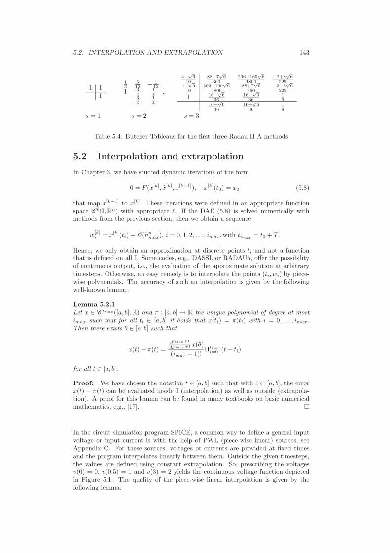
5.2. INTERPOLATION AND EXTRAPOLATION 143
1 11
,
13
512 − 1
121 3
414
34
14
,
4−√
610
88−7√
6360
296−169√
61800
−2+3√
6225
4+√
610
296+169√
61800
88+7√
6360
−2−3√
6225
1 16−√
636
16+√
636
19
16−√
636
16+√
636
19
s = 1 s = 2 s = 3
Table 5.4: Butcher Tableaus for the first three Radau II A methods
5.2 Interpolation and extrapolation
In Chapter 3, we have studied dynamic iterations of the form
0 = F (x[k], x[k], x[k−1]), x[k](t0) = x0 (5.8)
that map x[k−1] to x[k]. These iterations were defined in an appropriate functionspace C ℓ(I, Rn) with appropriate ℓ. If the DAE (5.8) is solved numerically withmethods from the previous section, then we obtain a sequence
w[k]i = x[k](ti) + O(hp
max), i = 0, 1, 2, . . . , imax, with timax= t0 + T.
Hence, we only obtain an approximation at discrete points ti and not a functionthat is defined on all I. Some codes, e.g., DASSL or RADAU5, offer the possibilityof continuous output, i.e., the evaluation of the approximate solution at arbitrarytimesteps. Otherwise, an easy remedy is to interpolate the points (ti, wi) by piece-wise polynomials. The accuracy of such an interpolation is given by the followingwell-known lemma.
Lemma 5.2.1Let x ∈ C imax([a, b], R) and π : [a, b] → R the unique polynomial of degree at mostimax such that for all ti ∈ [a, b] it holds that x(ti) = π(ti) with i = 0, . . . , imax.Then there exists θ ∈ [a, b] such that
x(t) − π(t) =dimax+1
dtimax+1 x(θ)
(imax + 1)!Πimax
i=0 (t − ti)
for all t ∈ [a, b].
Proof: We have chosen the notation t ∈ [a, b] such that with I ⊂ [a, b], the errorx(t) − π(t) can be evaluated inside I (interpolation) as well as outside (extrapola-tion). A proof for this lemma can be found in many textbooks on basic numericalmathematics, e.g., [17].
In the circuit simulation program SPICE, a common way to define a general inputvoltage or input current is with the help of PWL (piece-wise linear) sources, seeAppendix C. For these sources, voltages or currents are provided at fixed timesand the program interpolates linearly between them. Outside the given timesteps,the values are defined using constant extrapolation. So, prescribing the voltagesv(0) = 0, v(0.5) = 1 and v(3) = 2 yields the continuous voltage function depictedin Figure 5.1. The quality of the piece-wise linear interpolation is given by thefollowing lemma.

144CHAPTER 5. NUMERICAL ASPECTS OF DYNAMIC ITERATION METHODS
0 0.5 1 1.5 2 2.5 3 3.5 4−1
−0.5
0
0.5
1
1.5
2
2.5
3
t
volta
ge
PWL voltage source
Figure 5.1: PWL voltage source
Lemma 5.2.2Let t0 < t1 < · · · < timax
and x ∈ C 2([t0, timax], Rn). Let π ∈ C 0([t0, timax
], Rn)with π linear for t ∈ [ti, ti+1] for all i = 1, . . . , imax − 1. Then
‖x − π‖∞ ≤ h2max
8‖x‖∞
with
hmax = maxi=1,...,imax−1
(ti+1 − ti).
Proof: For every component xj and πj of x and π, respectively, we can applyLemma 5.2.1. Hence for t ∈ [ti, ti+1] it holds that there exists θ ∈ [ti, ti+1] suchthat
|xj(t) − πj(t)| =
∣∣∣∣xj(θ)
2(t − ti)(t − ti+1)
∣∣∣∣ .
For t ∈ [ti, ti+1], we have
|(t − ti)(t − ti+1)| = (t − ti)(ti+1 − t)
=(√
(t − ti)(ti+1 − t))2
.
Using the well-known inequality between the geometric and algebraic means, cf. [28],we obtain
|(t − ti)(t − ti+1)| =(√
(t − ti)(ti+1 − t))2
≤(
(ti+1 − ti)
2
)2
.
Hence with |xj(θ)| ≤ ‖x‖∞, we have
|xj(t) − πj(t)| ≤(ti+1 − ti)
2
8‖x‖∞

5.3. GLOBAL CONVERGENCE 145
for all j = 1, . . . , n and with the definition of hmax and the ‖·‖∞ norm, the assertionfollows.
Outside the interval I = [t0, timax], the following error bound holds.
Lemma 5.2.3Let x ∈ C 1([a, b], Rn) and π ∈ C ∞([a, b], Rn) with π ≡ x(a). Then
‖x − π‖∞ ≤ (b − a)‖x‖∞.
Proof: The proof follows directly from applying Lemma 5.2.1 componentwise tox − π and then using the definition of the ‖ · ‖∞ norm.
Remark 5.2.4 An analogous result to Lemma 5.2.3 is obtained for π ≡ x(b).
5.3 Global convergence
In this section, we will review the convergence results of Chapter 3, taking roundingerrors into account. Also, in Theorem 3.2.6, we only gave convergence results onone time interval [t0, t0 + T ]. Here, we will investigate error propagation from onetime window to another.Let [t0, te] be the considered full time interval. Let Ti > 0, i = 1, . . . , imax be thelengths of the time windows on which dynamic iteration is performed such that
te = t0 +
imax∑
i=1
Ti.
We define
t<j>0 = t0 +
j∑
i=1
Ti
and thus, the i-th time window will be [t<i>0 , t<i>
0 + Ti]. We will also call thesetime windows macro steps and the Ti macro stepsizes. We want to solve (5.8) onevery macro step. We write the k-th iterate of the DI process in the time window[t<i>
0 , t<i>0 + Ti] as x[k]<i>. Also, let x be the unique solution of
F (x, x, x) = 0, x(t0) = x0, (5.9)
with F as in (5.8). Then, x is a fixed point of the recurrence (5.8) and, thus,the required solution. We define x<i> as the restriction of x to the macro step[t<i>
0 , t<i>0 + Ti]. Also, we solve (5.8) numerically.
Let w[k]<i> ∈ C ([t<i>0 , t<i>
0 + Ti], Rn) be the numerical approximation to x[k]<i>.
Assumption 5.3.1 We will make the following simplifying assumptions.
• In each macro step, the iterates w[k]<i> with 0 ≤ k ≤ k<i>max are defined.
• The starting value in each iteration step w[k]<i>(t<i>0 ) is consistent.
• The starting iterate w[0]<i> is obtained as constant extrapolation of the nu-merical approximation of the last iterate at the end of the previous macrostep
w[0]<i>(t) = w[k<i−1>max ]<i−1>(t<i−1>
0 + Ti) for t ∈ [t<i>0 , t<i>
0 + Ti−1],
where k<i−1>max is the number of performed iterations in macro step (i − 1).

146CHAPTER 5. NUMERICAL ASPECTS OF DYNAMIC ITERATION METHODS
• On each macro step, we can transform (5.8) to an ODE of the form (3.7).
• On each macro step, we can define the interpolation error
ε[k]<i>max = max
j=1,...,jmax
‖w[k]<i>(tj) − w[k]<i>(tj)‖∞, (5.10)
where w[k]<i> is the unique exact solution of
0 = F (w[k]<i>,d
dtw[k]<i>, w[k−1]<i>), (5.11)
w[k]<i>(t<i>0 ) = w[0]<i>(t<i>
0 ), (5.12)
and w[k]<i> is the numerical approximation of w[k]<i> and tj are the time-points where w[k]<i> is evaluated.
• For each i ≥ 1, k ≥ 0, the normalized interpolation error
ε[k]<i>max
Ti
≤ Emax (5.13)
remains bounded.
• For each i ≥ 1 and k ≥ 0 we have
w[k]<i>(t<i>0 ) = w[k]<i>(t<i>
0 ) = w[0]<i>(t<i>0 ). (5.14)
We are going to construct an error bound that establishes a relation between theerrors in macro step i and (i−1). But first, we need to state a lemma that is similarto Theorem 3.2.6 but where we deliberately allow different starting values for thesequence of iterates and the fixed point.
Lemma 5.3.2Given a sequence x[k] ∈ C L (I, Rn), k = 1, . . . ,∞ with x[k] ∈ L1(I, R
n) defined bya differential difference equation
x[k] = ϕ(x[k], x[k−1], x[k−1]), (5.15)
where ϕ ∈ C 2(Rn × Rn × R
n, Rn). Let x[0] ∈ C 1(I, Rn) be a starting iterate and x0
an initial value s.t.
x[k](t0) = x0, k = 1, . . . ,∞.
Let x ∈ C 1(I, Rn) be a fixed point of (5.15). Then there exist constants α > 0 andL > 0 independent of k such that
‖x[k] − x‖∞,α ≤ L‖x[k−1] − x‖∞,α + 2e−αt0‖x0 − x(t0)‖∞.
Proof: Similar to the proof of Theorem 3.2.6, we define the integral operator
x[k](t) = x[k](t0) +
∫ t
t0
ϕ(x[k](τ ), x[k−1](τ ), x[k−1](τ ))dτ. (5.16)
The recurrence (5.16) is equivalent to (5.15). Hence, x also satisfies
x(t) = x(t0) +
∫ t
t0
ϕ(x(τ ), x(τ ), x(τ ))dτ.
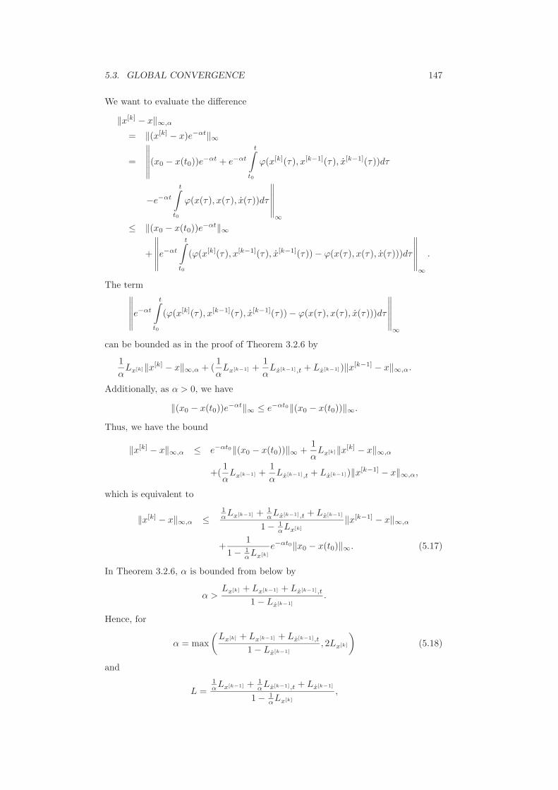
5.3. GLOBAL CONVERGENCE 147
We want to evaluate the difference
‖x[k] − x‖∞,α
= ‖(x[k] − x)e−αt‖∞
=
∥∥∥∥∥∥(x0 − x(t0))e
−αt + e−αt
t∫
t0
ϕ(x[k](τ ), x[k−1](τ ), x[k−1](τ ))dτ
−e−αt
t∫
t0
ϕ(x(τ ), x(τ ), x(τ ))dτ
∥∥∥∥∥∥∞
≤ ‖(x0 − x(t0))e−αt‖∞
+
∥∥∥∥∥∥e−αt
t∫
t0
(ϕ(x[k](τ ), x[k−1](τ ), x[k−1](τ )) − ϕ(x(τ ), x(τ ), x(τ )))dτ
∥∥∥∥∥∥∞
.
The term∥∥∥∥∥∥e−αt
t∫
t0
(ϕ(x[k](τ ), x[k−1](τ ), x[k−1](τ )) − ϕ(x(τ ), x(τ ), x(τ )))dτ
∥∥∥∥∥∥∞
can be bounded as in the proof of Theorem 3.2.6 by
1
αLx[k]‖x[k] − x‖∞,α + (
1
αLx[k−1] +
1
αLx[k−1],t + Lx[k−1])‖x[k−1] − x‖∞,α.
Additionally, as α > 0, we have
‖(x0 − x(t0))e−αt‖∞ ≤ e−αt0‖(x0 − x(t0))‖∞.
Thus, we have the bound
‖x[k] − x‖∞,α ≤ e−αt0‖(x0 − x(t0))‖∞ +1
αLx[k]‖x[k] − x‖∞,α
+(1
αLx[k−1] +
1
αLx[k−1],t + Lx[k−1])‖x[k−1] − x‖∞,α,
which is equivalent to
‖x[k] − x‖∞,α ≤1αLx[k−1] + 1
αLx[k−1],t + Lx[k−1]
1 − 1αLx[k]
‖x[k−1] − x‖∞,α
+1
1 − 1αLx[k]
e−αt0‖x0 − x(t0)‖∞. (5.17)
In Theorem 3.2.6, α is bounded from below by
α >Lx[k] + Lx[k−1] + Lx[k−1],t
1 − Lx[k−1]
.
Hence, for
α = max
(Lx[k] + Lx[k−1] + Lx[k−1],t
1 − Lx[k−1]
, 2Lx[k]
)(5.18)
and
L =1αLx[k−1] + 1
αLx[k−1],t + Lx[k−1]
1 − 1αLx[k]
,
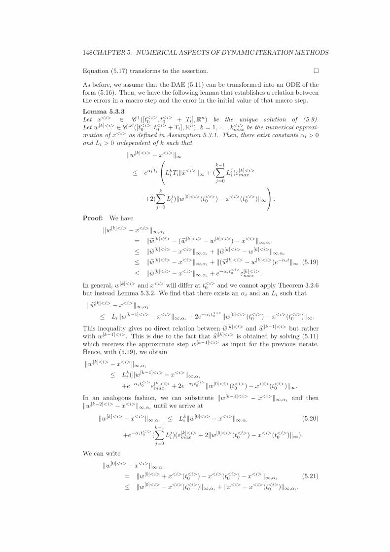
148CHAPTER 5. NUMERICAL ASPECTS OF DYNAMIC ITERATION METHODS
Equation (5.17) transforms to the assertion.
As before, we assume that the DAE (5.11) can be transformed into an ODE of theform (5.16). Then, we have the following lemma that establishes a relation betweenthe errors in a macro step and the error in the initial value of that macro step.
Lemma 5.3.3Let x<i> ∈ C 1([t<i>
0 , t<i>0 + Ti], R
n) be the unique solution of (5.9).Let w[k]<i> ∈ C L ([t<i>
0 , t<i>0 + Ti], R
n), k = 1, . . . , k<i>max be the numerical approxi-
mation of x<i> as defined in Assumption 5.3.1. Then, there exist constants αi > 0and Li > 0 independent of k such that
‖w[k]<i> − x<i>‖∞
≤ eαiTi
Lk
i Ti‖x<i>‖∞ + (k−1∑
j=0
Lji )ε
[k]<i>max
+2(k∑
j=0
Lji )‖w[0]<i>(t<i>
0 ) − x<i>(t<i>0 )‖∞
.
Proof: We have
‖w[k]<i> − x<i>‖∞,αi
= ‖w[k]<i> − (w[k]<i> − w[k]<i>) − x<i>‖∞,αi
≤ ‖w[k]<i> − x<i>‖∞,αi+ ‖w[k]<i> − w[k]<i>‖∞,αi
≤ ‖w[k]<i> − x<i>‖∞,αi+ ‖(w[k]<i> − w[k]<i>)e−αit‖∞ (5.19)
≤ ‖w[k]<i> − x<i>‖∞,αi+ e−αit
<i>0 ε[k]<i>
max .
In general, w[k]<i> and x<i> will differ at t<i>0 and we cannot apply Theorem 3.2.6
but instead Lemma 5.3.2. We find that there exists an αi and an Li such that
‖w[k]<i> − x<i>‖∞,αi
≤ Li‖w[k−1]<i> − x<i>‖∞,αi+ 2e−αit
<i>0 ‖w[0]<i>(t<i>
0 ) − x<i>(t<i>0 )‖∞.
This inequality gives no direct relation between w[k]<i> and w[k−1]<i> but ratherwith w[k−1]<i>. This is due to the fact that w[k]<i> is obtained by solving (5.11)which receives the approximate step w[k−1]<i> as input for the previous iterate.Hence, with (5.19), we obtain
‖w[k]<i> − x<i>‖∞,αi
≤ Lki (‖w[k−1]<i> − x<i>‖∞,αi
+e−αit<i>0 ε[k]<i>
max + 2e−αit<i>0 ‖w[0]<i>(t<i>
0 ) − x<i>(t<i>0 )‖∞.
In an analogous fashion, we can substitute ‖w[k−1]<i> − x<i>‖∞,αiand then
‖w[k−2]<i> − x<i>‖∞,αiuntil we arrive at
‖w[k]<i> − x<i>‖∞,αi≤ Lk
i ‖w[0]<i> − x<i>‖∞,αi(5.20)
+e−αit<i>0 (
k−1∑
j=0
Lji )(ε
[k]<i>max + 2‖w[0]<i>(t<i>
0 ) − x<i>(t<i>0 )‖∞).
We can write
‖w[0]<i> − x<i>‖∞,αi
= ‖w[0]<i> + x<i>(t<i>0 ) − x<i>(t<i>
0 ) − x<i>‖∞,αi(5.21)
≤ ‖w[0]<i> − x<i>(t<i>0 )‖∞,αi
+ ‖x<i> − x<i>(t<i>0 )‖∞,αi
.

5.3. GLOBAL CONVERGENCE 149
With Assumption 5.3.1, w[0]<i> is constant and we have
‖w[0]<i> − x<i>(t<i>0 )‖∞,αi
≤ e−αit<i>0 ‖w[0]<i>(t<i>
0 ) − x<i>(t<i>0 )‖∞
≤ 2e−αit<i>0 ‖w[0]<i>(t<i>
0 ) − x<i>(t<i>0 )‖∞.
Also,
‖x<i> − x<i>(t<i>0 )‖∞,αi
= ‖(x<i> − x<i>(t<i>0 ))e−αit‖∞
≤ e−αit<i>0 ‖(x<i> − x<i>(t<i>
0 ))‖∞.
With Lemma 5.2.3, this can be bounded by
‖x<i> − x<i>(t<i>0 )‖∞,αi
≤ e−αit<i>0 Ti‖x<i>‖∞. (5.22)
Also, in (5.20), the term ‖w[k]<i> − x<i>‖∞,αican be bounded from below as
‖w[k]<i> − x<i>‖∞,αi= ‖(w[k]<i> − x<i>)e−αit‖∞≥ e−αi(t
<i>0 +Ti)‖w[k]<i> − x<i>‖∞
Hence, together with (5.22) and (5.21), we have in (5.20) that
e−αi(t<i>0 +Ti)‖w[0]<i> − x<i>‖∞
≤ e−αit<i>0 Lk
i Ti‖x<i>‖∞ + e−αit<i>0 (
k−1∑
j=0
Lji )ε
[k]<i>max
+2e−αit<i>0 (
k∑
j=0
Lji )‖w[0]<i>(t<i>
0 ) − x<i>(t<i>0 )‖∞
and after multiplication with eαi(t<i>0 +Ti) we obtain
‖w[k]<i> − x<i>‖∞
≤ eαiTi
Lk
i Ti‖x<i>‖∞ + (k−1∑
j=0
Lji )ε
[k]<i>max (5.23)
+2(k∑
j=0
Lji )‖w[0]<i>(t<i>
0 ) − x<i>(t<i>0 )‖∞
which is the assertion.
With the help of Lemma 5.3.3, we can now state an error bound that is valid inevery macro step and every step of the DI. For simplification, we will furthermoreassume, that the DI is contractive on every macro step, i.e.,
Li < Lmax < 1.
Hence, all
cj :=1
1 − Lj
are well defined and positive. We furthermore define
bj := Lk<j>
max
j ‖x<j>‖∞ + cj
ε[k<i>
max]<j>max
Tj
.
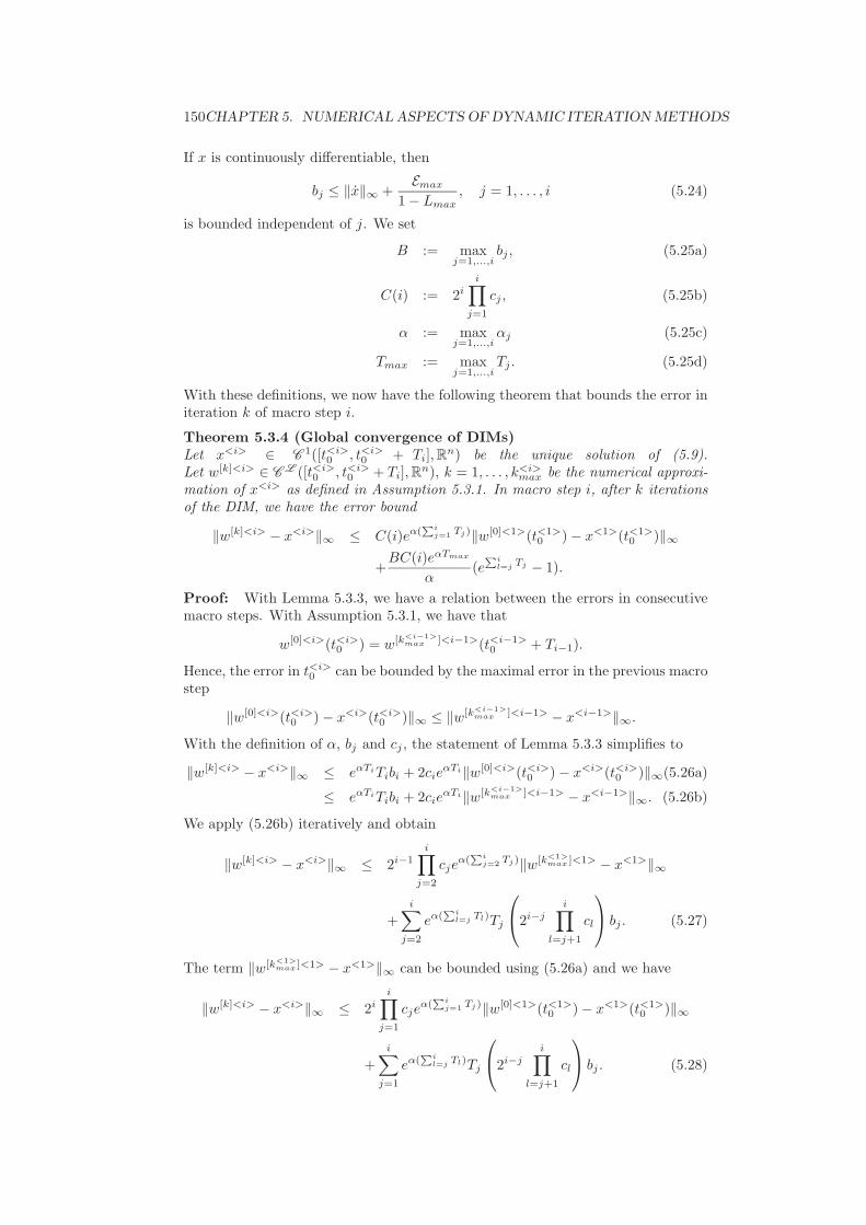
150CHAPTER 5. NUMERICAL ASPECTS OF DYNAMIC ITERATION METHODS
If x is continuously differentiable, then
bj ≤ ‖x‖∞ +Emax
1 − Lmax
, j = 1, . . . , i (5.24)
is bounded independent of j. We set
B := maxj=1,...,i
bj , (5.25a)
C(i) := 2i
i∏
j=1
cj , (5.25b)
α := maxj=1,...,i
αj (5.25c)
Tmax := maxj=1,...,i
Tj . (5.25d)
With these definitions, we now have the following theorem that bounds the error initeration k of macro step i.
Theorem 5.3.4 (Global convergence of DIMs)Let x<i> ∈ C 1([t<i>
0 , t<i>0 + Ti], R
n) be the unique solution of (5.9).Let w[k]<i> ∈ C L ([t<i>
0 , t<i>0 + Ti], R
n), k = 1, . . . , k<i>max be the numerical approxi-
mation of x<i> as defined in Assumption 5.3.1. In macro step i, after k iterationsof the DIM, we have the error bound
‖w[k]<i> − x<i>‖∞ ≤ C(i)eα(Pi
j=1 Tj)‖w[0]<1>(t<1>0 ) − x<1>(t<1>
0 )‖∞
+BC(i)eαTmax
α(e
Pil=j
Tj − 1).
Proof: With Lemma 5.3.3, we have a relation between the errors in consecutivemacro steps. With Assumption 5.3.1, we have that
w[0]<i>(t<i>0 ) = w[k<i−1>
max ]<i−1>(t<i−1>0 + Ti−1).
Hence, the error in t<i>0 can be bounded by the maximal error in the previous macro
step
‖w[0]<i>(t<i>0 ) − x<i>(t<i>
0 )‖∞ ≤ ‖w[k<i−1>max ]<i−1> − x<i−1>‖∞.
With the definition of α, bj and cj , the statement of Lemma 5.3.3 simplifies to
‖w[k]<i> − x<i>‖∞ ≤ eαTiTibi + 2cieαTi‖w[0]<i>(t<i>
0 ) − x<i>(t<i>0 )‖∞(5.26a)
≤ eαTiTibi + 2cieαTi‖w[k<i−1>
max ]<i−1> − x<i−1>‖∞. (5.26b)
We apply (5.26b) iteratively and obtain
‖w[k]<i> − x<i>‖∞ ≤ 2i−1i∏
j=2
cjeα(
Pij=2 Tj)‖w[k<1>
max ]<1> − x<1>‖∞
+i∑
j=2
eα(Pi
l=j Tl)Tj
2i−j
i∏
l=j+1
cl
bj . (5.27)
The term ‖w[k<1>max ]<1> − x<1>‖∞ can be bounded using (5.26a) and we have
‖w[k]<i> − x<i>‖∞ ≤ 2i
i∏
j=1
cjeα(
Pij=1 Tj)‖w[0]<1>(t<1>
0 ) − x<1>(t<1>0 )‖∞
+i∑
j=1
eα(Pi
l=j Tl)Tj
2i−j
i∏
l=j+1
cl
bj . (5.28)

5.3. GLOBAL CONVERGENCE 151
Then, with (5.25a) and (5.25b)
‖w[k]<i> − x<i>‖∞ ≤ C(i)eα(Pi
j=1 Tj)‖w[0]<1>(t<1>0 ) − x<1>(t<1>
0 )‖∞
+BC(i)
i∑
j=1
eα(Pi
l=jTl)Tj . (5.29)
We set
Θj :=
i∑
l=i−j+1
Tl, j = 0, . . . , i,
i.e. Θ0 = 0, Θ1 = Ti, . . . , Θi =∑i
j=1 Tj . Then,
i∑
j=1
eα(Pi
l=j Tl)Tj =i∑
j=1
eαΘj (Θj − Θj−1). (5.30)
As α > 0, the function eαt is strictly increasing and we have an approximation tothe integral
∫ Θi
0
eαtdt,
by lower sums as
i∑
j=1
eαΘj−1(Θj − Θj−1) ≤∫ Θi
0
eαtdt.
With (5.25d), we have
Θj − Tmax ≤ Θj−1 ≤ Θj
and
i∑
j=1
eαΘj−Tmax(Θj − Θj−1) = e−αTmax
i∑
j=1
eαΘj (Θj − Θj−1)
≤ e−αTmax
i∑
j=1
eαΘj (Θj − Θj−1).
Thus, for (5.30), we obtain
i∑
j=1
eαΘj (Θj − Θj−1 ≤ eαTmax
∫ Θi
0
eαtdt
≤ eαTmax
α(eΘi − 1).
With the definition of Θi =∑i
j=1 Tj , the assertion follows.
The error bound of Theorem 5.3.4 has many implications. First, the error dependsexponentially on the total length of the computation interval, i.e., the sum of allmacro step sizes. The factor α of this exponential growth is related to the valuesLj by Equation (5.18). Hence, slow convergence also implies larger global errors.

152CHAPTER 5. NUMERICAL ASPECTS OF DYNAMIC ITERATION METHODS
0
Ti Ti−1 T1
Θ1 Θ2 Θi−1 Θi
eαt
Figure 5.2: Approximation of the integral by lower sums
Besides the length of the computation interval, also the number of macro stepsenters the error in the term C(i). The other parameters that influence the globalerror are the error in the initial value ‖w[0]<1>(t<1>
0 ) − x<1>(t<1>0 )‖∞ and the
value B. Of these two, only B is influenced by the numerical methods used forintegration of the DAEs and interpolation of the resulting approximate solution.With the definition of B in (5.25a), we have that
B = maxj=1,...,i
Lk<j>
max
j ‖x<j>‖∞ + cj
ε[k<j>
max ]<j>max
Tj
.
This equation implies that the number of DI steps k<j>max in one macro step has to
be chosen depending on the rate of convergence Lj and the value ‖x<j>‖∞. Forvery small Lj , the number of iterations may be chosen very small, whereas a large‖x<j>‖∞ may require additional DI steps. Independent of the number of DI steps,the error in each step is bounded by
cj
ε[k<j>
max ]<j>max
Tj
.
Hence, the inaccuracies of the numerical approximation effectively limit the maximal
reachable accuracy. With the definition of ε[k]<j>max , (5.10), we see that the errors
from interpolation and integration are independent. If we used piecewise linearinterpolation and the BDF method of order 3, then with Lemma 5.2.2 and Theorem5.1.5, the error is
‖w − w‖ = O(h2max) + O(h3
max) = O(h2max).
Hence, if we use piecewise linear interpolation, then it is sufficient to use an inte-gration method of order 2 like the BDF-2 method or the trapezoidal rule.
5.4 Macro stepsize selection
If we consider purely algebraic recurrences like
x[k] = Lx[k−1]

5.4. MACRO STEPSIZE SELECTION 153
with, e.g., x[0] = 1, then the difference to the correct solution is
x[k] − x = Lk.
This error development is independent of the length of the computation interval.However, for a quasi-instantaneously convergent DIM, the situation is usually dif-ferent. Consider the simple example of a quasi-instantaneously convergent DIM
x[k] = −x[k−1], x[k](0) = 1, x[0] = 1. (5.31)
The limit of this recurrence is x = e−t. If we iterate (5.31) on the interval I = [0, 2],then the first few iterates are
x[0] = 1,
x[1] = 1 − t,
x[2] = 1 − t +t2
2,
x[3] = 1 − t +t2
2− t3
6.
In Figure 5.3 the function graphs of x[0], . . . , x[3] as well as the errors with respect tox are depicted. It can easily be seen that at t = 1, the errors are rapidly decreasingwhile at t = 2, the error first increases and only with the second iteration, it slowlystarts to decrease. However, if we divide the interval I = [0, 1] ∪ [1, 2] = I1 ∪ I2 andrestart the DI at t = 1 after a number of iterations, the error behaviour over thewhole interval I is much better. In Figure 5.4, the iterates and errors for a DI withtwo macro steps and a fixed number of dynamic iterates per macro step is plotted.It can be observed that the errors in the second sub-interval I2 are much smallerthan in the case of the integration over all I. It also has to be noted that the totalnumber of iteration steps with two macro steps is comparable to the case of onemacro step. If we choose constant stepsizes for the integration, then these numbersare even equal. Hence, using small macro steps seems to yield more accurate re-sults at virtually no extra cost. This, however, is misleading as with the numberof macro steps, the amount of data that is transferred between different solversincreases. Also, usually a DAE solver produces some overhead computation timefor initialization purposes. Using very small macro steps multiplies this overheadand makes the whole DIM ineffective.
Observation 5.4.1 It can be observed that the length of the interval where thesolution x[k] of a DIM differs by less than a given tol from the correct solution xgrows approximately linearly with k and becomes independent of the value tol withincreasing k.
Example 5.4.2 Consider a simple example. We want to solve
x[k] = cx[k−1], x[k](0) = 1, x[0] ≡ 1 (5.32)
on the interval I = [0, T ]. With Theorem 3.1.3, this DIM converges and the limitingsolution is x(t) = ect. Let X = L (x), X [k] = L (x[k]). Then, in frequency domain,(5.32) becomes
sX [k] = cX [k−1] + 1,
X [k] =c
sX [k−1] +
1
s.

154CHAPTER 5. NUMERICAL ASPECTS OF DYNAMIC ITERATION METHODS
0 0.2 0.4 0.6 0.8 1 1.2 1.4 1.6 1.8 2−1
−0.8
−0.6
−0.4
−0.2
0
0.2
0.4
0.6
0.8
1
t
x
iterates
x
x[0]
x[1]
x[2]
x[3]
0 0.2 0.4 0.6 0.8 1 1.2 1.4 1.6 1.8 20
0.2
0.4
0.6
0.8
1
1.2
1.4
t
|x−
x[i]|
errors
x[0]
x[1]
x[2]
x[3]
Figure 5.3: The first iterates and errors for the DIM (5.31)

5.4. MACRO STEPSIZE SELECTION 155
0 0.2 0.4 0.6 0.8 1 1.2 1.4 1.6 1.8 20
0.1
0.2
0.3
0.4
0.5
0.6
0.7
0.8
0.9
1
t
x
iterates
x
0 steps
1 step
2 steps
3 steps
0 0.2 0.4 0.6 0.8 1 1.2 1.4 1.6 1.8 20
0.1
0.2
0.3
0.4
0.5
0.6
0.7
0.8
0.9errors
t
|x−
x[i]|
0 steps1 step2 steps3 steps
Figure 5.4: The first iterates and errors for the DIM (5.31) with two macro steps

156CHAPTER 5. NUMERICAL ASPECTS OF DYNAMIC ITERATION METHODS
With L (x[0]) = L (1) = s−1, we can determine X [k] explicitly:
X [k] =( c
s
)k
X [0] +1
s
k−1∑
i=0
( c
s
)i
=1
s
k∑
i=0
( c
s
)i
=1
s
1 −(
cs
)k+1
1 − cs
=1 −
(cs
)k+1
s − c.
We have X = L (x) = L (ect) = 1s−c
. Hence
X − X [k] = ck+1 1
sk+1
1
s − c.
In state space, we then have
x − x[k] = ck+1(tk
k!∗ ect)
= ck+1
t∫
0
τk
k!· ec(t−τ)dτ
≤ (ct)k+1
(k + 1)!· K (5.33)
where K = max(1, ecT ). We use Stirling’s formula
k! ≈(
k
e
)k √2πk,
cf. [20], with the further simplification that
k! ≈(
k
e
)k
for sufficiently large k. In (5.33), we then obtain
x − x[k] /(ct)k+1
(k+1
e
)k+1· K
/
(cte
k + 1
)k+1
· K.
If we want |x − x[k]| < tol, then
∣∣∣∣cte
k + 1
∣∣∣∣k+1
· K < tol,
∣∣∣∣cte
k + 1
∣∣∣∣ <k+1
√tol
K,
t <
∣∣∣∣k + 1
ce
∣∣∣∣k+1
√tol
K.

5.4. MACRO STEPSIZE SELECTION 157
For large values of k, the root term approaches 1 and we have
t /
∣∣∣∣k + 1
ce
∣∣∣∣ =1
|c|e (k + 1). (5.34)
This equation implies that the length of the interval where the difference of x[k]
and x is smaller than tol is almost proportional to k and independent of tol. Thisbehaviour can be observed in the numerical experiments in the following chapter.It also implies that this interval increases its length by 1
|c|e in every iteration step.
Thus, convergence is slower for large values of |c|.
With Observation 5.4.1, the different behaviour in Figures 5.3 and 5.4 can be ex-plained. In the case where the interval is divided into two subintervals of length 1,a number of DI steps is performed on each macro step that is equal to the numberof iterations that before were performed on the whole interval [0, 2]. In total, twicethe number of DI steps is performed, when the computation is done on two macrosteps. Thus, with Observation 5.4.1, the length of the interval, where the solutionis sufficiently accurate is about twice as long as in the case of only one macro step.In order to have comparable accuracies, an equal overall number of DI steps has tobe performed, regardless of macro step sizes. We have seen before that with smallsubinterval lengths, the computational effort for the integration of the ODEs orDAEs, respectively, can be reduced. Conversely, small subintervals lead to a largenumber of subintervals and increased communication overhead. Hence, we want tochoose macro step sizes in such a way that the effort for numerical integration iskept low by choosing sufficiently small macro steps while making them large enoughto reduce the communication load.
Error estimation
We will restrict our considerations to quasi-instantaneously convergent systems, asno gains can be expected from macro step size control for DI methods with slowconvergence. As we have seen in the previous section, using higher order integrationand interpolation methods has only a limited influence on the accuracy of a DI step.If in (5.24), the errors from integration and interpolation are sufficiently small, thenthe overall error is mainly defined by Lj and the number of DI steps in that macrostep. For quasi-instantaneous convergence, we may assume very small Lj , hencewithin a neighborhood of the starting point, the next iterate can be seen as areasonable approximation of the exact solution. As the (k + 1)st iterate is notavailable for the computation of the kth iterate, we will base stepsize control on thedifference
x[k] − x[k−1]
which approximates the error to the exact solution in step (k − 1). We define anerror estimate ǫ[k]<i> as
ǫ[k]<i>j = ‖w[k]<i>
j − π(w[k−1]<i>, tj)‖, k = 1, . . . , k<i>max, (5.35)
where w[k]<i>j = w[k]<i>(tj) with w[k]<i> as defined in Assumption 5.3.1 and
π(w[k−1]<i>, t∗) is a piecewise linear interpolant of w[k−1]<i> at t∗. The values
ǫ[k]<i>j are only defined at the timesteps tj , where the numerical approximation
w[k]<i>(tj) is evaluated. With variable stepsizes, these timesteps usually do notcoincide with the steps in the previous DI step. Hence, in order to calculate anerror estimate at tj , we have to interpolate w[k−1]<i> at tj . As the initial values

158CHAPTER 5. NUMERICAL ASPECTS OF DYNAMIC ITERATION METHODS
w[k]<i>0 and w
[k−1]<i>0 are identical, we have that ǫ
[k]<i>0 = 0. We now check for
which index jtol the error criterion
ǫ[k]<i>j < RTOL · w[k]<i>j + ATOL + TTOL(tj − t<i>
0 ), j = 1, 2, . . . (5.36)
is breached for the first time. Here, RTOL and ATOL stand for relative and ab-solute error tolerances, respectively and TTOL is an error factor depending on thelength of the considered macro step. The length of the interval [t0, tj−1] where(5.36) is fulfilled, Ti, is assumed to be the length of a macro step in which a DIMconverges up to some tolerance within k steps. Then, DI for that macro step isstopped and the remainder of the interval for t > t<i>
0 + Ti is ignored. The DIMis then restarted for a new macro step of initial length βTi. This constant β > 1 isnecessary or the macro step sizes would only stagnate or decrease. In order to allowan increase of macro step sizes, the initial guess for Ti+1 is chosen deliberately largerthan Ti. A good choice is 1.2 ≤ β ≤ 2. A too small β means that the controller isincapable of rapid adaption, while a large β incurs the risk that large parts of theinterval are ignored after the interval of convergence has been found, and thus, muchcomputational effort is wasted. The whole procedure of error control is formulatedin Algorithm 4. This algorithm computes at most kmax DI steps and checks inevery macro step until which timestep the error criterion (5.36) is satisfied. In DIstep kmax, the length of the interval where (5.36) is fulfilled is used as final macrostep size Ti. If the desired accuracy is achieved over the whole interval in less thankmax iterations, then the DI process is aborted prematurely. The next macro stepsize Ti+1 is based on the obtained Ti. As a precaution, we set a minimal and amaximal macro step size. The minimal step size guarantees that the step size doesnot converge to zero making the solution process stagnate. The maximal step sizeensures that the macro step does not go beyond the whole computation interval. Ifthe error criterion fails already at j = 1, then Ti would be set to 0. Thus, in Line2, a warning is issued and as an exception, j is set to 2. The approximate solutionon the macro step is appended to the previously known solution. A new startingiterate is defined, e.g. by constant extrapolation of the last accepted solution valuein macro step i. Then, the process can be repeated for the next macro step.
Remark 5.4.3 Another approach to error control is to keep macro step sizes con-stant and to iterate until an error criterion is achieved over the full interval. Thisapproach, however has difficulties reacting to changing convergence behaviour andwill, thus, not be considered further.
5.5 Conclusion
In this chapter, we have investigated the aspects of determining the iterates of aDIM numerically. After stating some basic facts about numerical integration ofODEs and DAEs as well as some error bounds for interpolation and extrapolationof functions, we have given an error bound that relates the global error of a DIapproximation to the rate of convergence and the number of iterations in macrosteps, the length of the computation interval and local approximation errors. Theneed for a DIM that is efficient, even for changing convergence behaviour, led to theconstruction of a macro step size controller. A rather heuristic investigation of asimple test example revealed that macro step size control is not likely to dramaticallyreduce the overall number of DI steps. However, it ensures that the macro stepsare sufficiently short such that convergence of the DIM can be expected within areasonable number of DI steps. Hence, unnecessary computational effort, e.g., fornumerical integration is avoided.

5.5. CONCLUSION 159
Algorithm 4: Macro step size controller
Input : initial guess for macro step size Ti, initial iterate x[0]<i> for macrostep i
Output: effective macro step size Ti, approximate solution on macro step i,initial guess for macro step size Ti+1, initial iterate x[0]<i+1>
beginSet k=1while k ≤ kmax do1
Compute approximate solution w[k]<i> at timestepst0 = t<i>
0 , . . . , tjmax= t<i>
0 + Ti.Compute interpolation π(w[k−1]<i>, tj) at the timesteps t0, . . . , tjmax
.
Compute error estimate ǫ[k]<i>j , j = 0, . . . , jmax by (5.35).
foreach j ≤ jmax do
if ǫ[k]<i>j ≥ RTOL
tj−t<i>0
+ ATOL then
Set k := k + 1Proceed with Line 1.
Proceed with Line 2.if j = 1 then2
Issue WARNING.Set j := 2.
Set w[k]<i> := w[k]<i>
l j−1l=0 .
Set Ti := tj−1 − t0.Set Ti+1 := βTi.if Ti+1 < HMIN then
Set Ti+1 := HMIN .
if Ti+1 > HMAX thenSet Ti+1 := HMAX.
Set x[0]<i+1> = w[k]<i>j−1 .
end

160CHAPTER 5. NUMERICAL ASPECTS OF DYNAMIC ITERATION METHODS

Chapter 6
Numerical examples
In this chapter, we will mainly consider two examples of a rectifier circuit, an elec-trical circuit that is used to transform an alternating supply voltage into a unidirec-tional voltage. These circuits usually contain a diode to allow only unidirectionalcurrent-flow. Diodes and other semiconductor devices usually have an internal ca-pacitance that also has to be considered in the model. We will split these examplecircuits such that the diode forms one subcircuit and the remainder of the rectifiercircuit forms another subcircuit. In Section 6.1, the semiconductor will be modelledby a simple lumped element as in Definition 2.5.1. In this way, the diode subcircuitis governed by a nonlinear equation while the other subcircuit is represented by alinear DAE. Then, in Section 6.2, we will study the approximation quality of theDIM for a linearized diode model where an exact solution can be determined. InSection 6.3, we simulate the diode using a distributed model. The arising equationsfor the semiconductor are partial differential equations (PDEs). We will show, howdifferent solvers for PDEs and lumped circuits can be combined using the DIMapproach. In Section 6.4, we extend the example from Section 6.3 to a full-wave-or bridge-rectifier containing four diodes. The simulations of circuits with lumpedelements are carried out using SPICE-3f5, see Appendix C. Within one iteration ofthe DIM, one subcircuit is simulated and the potentials at splitting nodes and thecurrents in coupling sources are saved to disk and then automatically inserted intothe netlist file of the other subcircuits with the help of a Perl script. Then, thisprocess is repeated for the other subcircuits. The SPICE simulations are invokedby a Matlab script. This program also performs the error estimation, macro stepsize control and generates the graphical output.The simulation of the distributed diode model in Sections 6.3 and 6.4 is carried outby a Matlab routine developed at Johannes Gutenberg-Universitat Mainz, cf. [21].All computations were carried out on Pentium 4 workstations with 1 GB of RAMand Matlab R2007b. For simplicity, all considered quantities are assumed dimen-sionless.
6.1 Rectifier with lumped elements
We will first consider the rectifier circuit in Figure 6.1. This circuit contains a volt-age source, a resistive load and a semiconductor diode with a small parallel capac-itance. The corresponding MNA equations are
[0 00 C
] [e1
e2
]+
[G −G−G G
] [e1
e2
]+
[0
g(e2)
]+
[10
]jV = 0, (6.1a)
e1 = v, (6.1b)
161
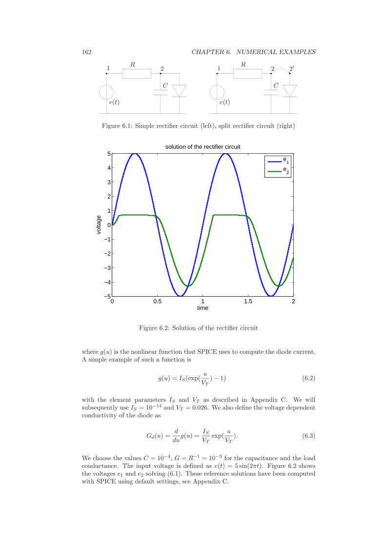
162 CHAPTER 6. NUMERICAL EXAMPLES
1 2
C
R
v(t)
1 2 2′
C
R
v(t)
Figure 6.1: Simple rectifier circuit (left), split rectifier circuit (right)
0 0.5 1 1.5 2−5
−4
−3
−2
−1
0
1
2
3
4
5solution of the rectifier circuit
time
volta
ge
e
1
e2
Figure 6.2: Solution of the rectifier circuit
where g(u) is the nonlinear function that SPICE uses to compute the diode current.A simple example of such a function is
g(u) = IS(exp(u
VT
) − 1) (6.2)
with the element parameters IS and VT as described in Appendix C. We willsubsequently use IS = 10−14 and VT = 0.026. We also define the voltage dependentconductivity of the diode as
Gd(u) =d
dug(u) =
IS
VT
exp(u
VT
). (6.3)
We choose the values C = 10−4, G = R−1 = 10−3 for the capacitance and the loadconductance. The input voltage is defined as v(t) = 5 sin(2πt). Figure 6.2 showsthe voltages e1 and e2 solving (6.1). These reference solutions have been computedwith SPICE using default settings, see Appendix C.

6.1. RECTIFIER WITH LUMPED ELEMENTS 163
−1 2 2′ 2′′
C
R
v(t)
GdGd
Figure 6.3: Augmented split rectifier circuit
If we split this circuit as in Figure 6.1, then, the DIM can be written as follows
[0 00 10−4
] [e1
e2
][k]
+
[10−3 −10−3
−10−3 10−3
] [e1
e2
][k]
+
[10
]j[k]V =
[01
]j[k−1]K , (6.4a)
e[k]1 = 5 sin(2πt) (6.4b)
and
g(e′[k]2 ) + j
[k]K = 0, (6.4c)
e′[k]2 = e
[k]2 . (6.4d)
The conductance of the diode varies from approximately Gd(−5) ≈ 1 · 10−96 toGd(5) ≈ 1 · 1071. The capacitance C on the side of the coupling current sourceguarantees convergence in the analytical sense. However, the speed of convergenceis still largely determined by the relation of the resistive elements. Hence, forGd(e
′2)/G > 1, convergence is very fast and for Gd(e
′2)/G < 1 convergence is very
slow and only observable for very short macro steps, see Observation 5.4.1. We willtry to improve this behaviour with the enforced convergence strategy of Algorithm2, applied to the resistive part of the circuit only. We introduce an additionalconductance that models the behaviour of the diode in parallel to the couplingcurrent source and add a third subcircuit to compensate for the extra element.The additional conductance is the conductance Gd(θi) of the diode evaluated atthe beginning θi of macro step i. In this way, the macro step size controller alsodetermines when a new Gd(·) should be computed. Figure 6.3 shows a graphicalrepresentation of the augmented coupled circuit. The small minus sign means thatthe negative coupling current from node 2′′ is introduced into node 2.
The new DIM equations are then
[0 00 10−4
] [e1
e2
][k]
+
[10−3 −10−3
−10−3 10−3 + Gd(θi)
] [e1
e2
][k]
+
[10
]j[k]V =
[0 01 −1
] [jK
j′K
][k−1]
, (6.5a)
e[k]1 = 5 sin(2πt) (6.5b)

164 CHAPTER 6. NUMERICAL EXAMPLES
and
g(e′[k]2 ) + j
[k]K = 0, (6.5c)
e′[k]2 = e
[k]2 , (6.5d)
Gd(θi)e′′[k]2 + j
′[k]K = 0, (6.5e)
e′′[k]2 = e
[k]2 . (6.5f)
We iterate the two DI processes (6.4) and (6.5) with a macro step size controller
as in Algorithm 4. The initial macro step size is T1 = 10−2 and the computationinterval is I = [0, 2]. This interval contains two full periods of the supply voltage.We use the initial values e1(0) = e2(0) = jV (0) = 0. We set RTOL = 0 and varyTTOL = ATOL = tol as well as the maximal number of DI steps kmax. Addition-ally, the maximum length of one DI step is limited to 0.1. The stepsize increasefactor β in Algorithm 4 is set to β = 2. This was necessary, as in the acceleratedcase, the stepsize controller sometimes overestimated the next stepsize and SPICEproduced meaningless results on the too large step.
The obtained results are compiled in Table 6.1. The stated errors are the maximumabsolute differences between the computed voltages and the voltages in a SPICEreference solution.Figure 6.4 shows that the solution obtained by the non-accelerated DIM fortol = 10−2 and kmax = 2 fits well to the reference solution. However, a zoominto the interval [0.2, 0.3] shows that the DI solution oscillates rapidly around thereference solution. The magnitude of these oscillations lies well within the spec-ified tolerance of 10−2. The automatically chosen macro step sizes for the sameparameter setting are shown in Figure 6.5. It can be observed that the step sizecontroller chooses very small step sizes when the diode enters the conducting range[0.1, 0.5] ∪ [1.1, 1.5]. The transition from large stepsizes to small ones goes veryabruptly. The change from small to large stepsizes is limited by the increase factorβ between consecutive step sizes. In this example, when the diode leaves the con-ducting range and enters the reverse mode, the macro steps can be chosen muchlarger and the controller reacts relatively fast.We can draw a number of conclusions from the results in Table 6.1 and the efficiencyplot in Figure 6.6. We see that the total computation time per parameter settingis roughly proportional to the number of SPICE calls. The total time per SPICEcall is approximately 0.4s. The effective integration time needed by SPICE lies inthe magnitude of 0.01s, see Figure 6.7. The remainder is used for the setup of theequations, for reading the computed voltages and currents, for adapting the netlistsfor the next iteration step and for other administration tasks such as error estima-tion. Currently, this is done in Matlab which facilitates the control of the SPICEcalls but produces costly screen outputs. Other background processes may also slowdown the computation. Hence, for benchmarking purposes we will use the numberof SPICE calls as reference because this number is machine independent. It has tobe mentioned at this point, that the computation of the reference solution also tookless than a second of computer time, while some of the presented simulations takehours. However, this section gives a benchmark example for the split simulation ofan electrical circuit. In order to show advantageous behaviour compared to mono-lithic simulation, other larger examples would have to be considered.It can be seen that the simulations with convergence acceleration are usually dra-matically faster than their non-accelerated counterparts, despite the fact that threesystems have to be simulated instead of only two. However, for low tolerances,the obtained results show large errors. In the non-accelerated case, the errors are
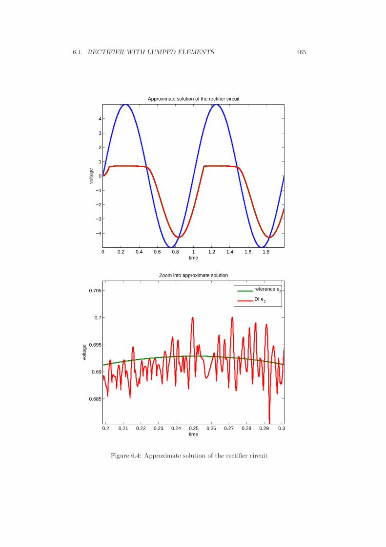
6.1. RECTIFIER WITH LUMPED ELEMENTS 165
0 0.2 0.4 0.6 0.8 1 1.2 1.4 1.6 1.8
−4
−3
−2
−1
0
1
2
3
4
time
volta
ge
Approximate solution of the rectifier circuit
0.2 0.21 0.22 0.23 0.24 0.25 0.26 0.27 0.28 0.29 0.3
0.685
0.69
0.695
0.7
0.705
time
volta
ge
Zoom into approximate solution
reference e2
DI e2
Figure 6.4: Approximate solution of the rectifier circuit
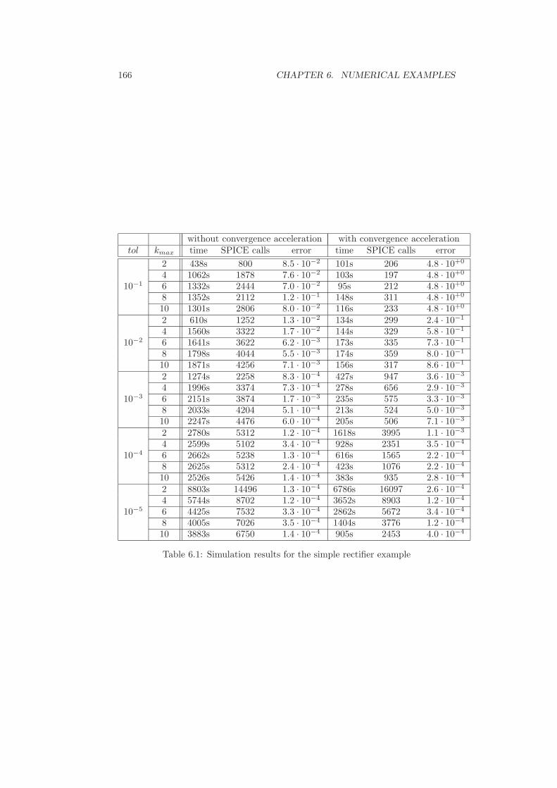
166 CHAPTER 6. NUMERICAL EXAMPLES
without convergence acceleration with convergence accelerationtol kmax time SPICE calls error time SPICE calls error
10−1
2 438s 800 8.5 · 10−2 101s 206 4.8 · 10+0
4 1062s 1878 7.6 · 10−2 103s 197 4.8 · 10+0
6 1332s 2444 7.0 · 10−2 95s 212 4.8 · 10+0
8 1352s 2112 1.2 · 10−1 148s 311 4.8 · 10+0
10 1301s 2806 8.0 · 10−2 116s 233 4.8 · 10+0
10−2
2 610s 1252 1.3 · 10−2 134s 299 2.4 · 10−1
4 1560s 3322 1.7 · 10−2 144s 329 5.8 · 10−1
6 1641s 3622 6.2 · 10−3 173s 335 7.3 · 10−1
8 1798s 4044 5.5 · 10−3 174s 359 8.0 · 10−1
10 1871s 4256 7.1 · 10−3 156s 317 8.6 · 10−1
10−3
2 1274s 2258 8.3 · 10−4 427s 947 3.6 · 10−3
4 1996s 3374 7.3 · 10−4 278s 656 2.9 · 10−3
6 2151s 3874 1.7 · 10−3 235s 575 3.3 · 10−3
8 2033s 4204 5.1 · 10−4 213s 524 5.0 · 10−3
10 2247s 4476 6.0 · 10−4 205s 506 7.1 · 10−3
10−4
2 2780s 5312 1.2 · 10−4 1618s 3995 1.1 · 10−3
4 2599s 5102 3.4 · 10−4 928s 2351 3.5 · 10−4
6 2662s 5238 1.3 · 10−4 616s 1565 2.2 · 10−4
8 2625s 5312 2.4 · 10−4 423s 1076 2.2 · 10−4
10 2526s 5426 1.4 · 10−4 383s 935 2.8 · 10−4
10−5
2 8803s 14496 1.3 · 10−4 6786s 16097 2.6 · 10−4
4 5744s 8702 1.2 · 10−4 3652s 8903 1.2 · 10−4
6 4425s 7532 3.3 · 10−4 2862s 5672 3.4 · 10−4
8 4005s 7026 3.5 · 10−4 1404s 3776 1.2 · 10−4
10 3883s 6750 1.4 · 10−4 905s 2453 4.0 · 10−4
Table 6.1: Simulation results for the simple rectifier example

6.1. RECTIFIER WITH LUMPED ELEMENTS 167
0 0.2 0.4 0.6 0.8 1 1.2 1.4 1.6 1.8 20
0.02
0.04
0.06
0.08
0.1
0.12
time
step
size
stepsizes for tol=10−2, kmax
=5
Figure 6.5: Macro step sizes for the rectifier circuit
well within the given tolerances. Only for tol = 10−5, the error bounds are notkept anymore. It cannot be determined if this is due to the DI process or a possi-bly inaccurate reference solution. This topic will be addressed in the next section.Starting with a tolerance of 10−3, the DI process with convergence accelerationproduces results of comparable accuracy with often significantly less SPICE calls.Another observation is that for low tolerances, the total number of SPICE invoca-tions rises with the maximal number of iterations per macro step kmax. For highertolerances, the opposite behaviour occurs. There exists a turning point in the toler-ances, where this behaviour switches. For non-accelerated iterations, the tolerance,where the number of SPICE calls is roughly independent of kmax is approximately10−4. In the case of convergence acceleration, this happens for tol = 10−2. Thiscan also be observed in Figure 6.6 where in the non-accelerated case, the settingkmax = 2 is the most efficient for tolerances tol ≥ 10−4. However, in the acceler-ated case, this is only true for tol ≥ 10−2. For smaller tolerances, a low number ofiterations per macro step quickly becomes very costly and, thus, inefficient.The standard accuracy requirement for voltages in SPICE is an error of less than1mV = 0.001V . In the non-accelerated case, the fastest simulation that fulfills thisaccuracy requirement is for tol = 10−3 and kmax = 2. In the accelerated case, thefastest simulation was for tol = 10−4 and kmax = 10, where probably kmax > 10would produce even better results. It is, thus, not possible to state an optimal num-ber of iterations per macro step. Also, in addition to the macro stepsize controller,controlling the number of iteration steps would be desirable. As a rule of thumb,we may suggest that in order to reach a certain accuracy, the tolerance for theaccelerated case should be chosen one order of magnitude smaller than the desiredaccuracy and the number of iterations per macro step should be about 10. It canalso be stated, that for a relatively large number of iterations per step, the overallcosts change very little, depending on the required accuracy. This last observation

168 CHAPTER 6. NUMERICAL EXAMPLES
102
103
104
105
10−4
10−3
10−2
10−1
100
101
number of SPICE calls
erro
r
efficiency: rectifier circuit
k
max=2
kmax
=10
tol=1e−1tol=1e−2tol=1e−3tol=1e−4tol=1e−5k
max=2
kmax
=10
tol=1e−1tol=1e−2tol=1e−3tol=1e−4tol=1e−5
Figure 6.6: Efficiency plot for the rectifier circuit with and without convergenceacceleration
Circuit: *subsystem 1 of circ_d
Warning: Source i_coup_2 has no DC value, transient time 0 value used
Warning: vin: no DC value, transient time 0 value used
CPU time since last call: 0.008 seconds.
Total CPU time: 0.008 seconds.
Figure 6.7: Sample SPICE output
coincides well with the statement of Observation 5.4.1.
6.2 Rectifier in conducting direction
In the previous section, we did only investigate the exactness of the solution obtainedby DI by comparing it to the SPICE approximation of the solution of (6.1). Thisis due to the fact that no explicit solution of (6.1) can be computed and there existno exact error bounds on solutions computed by SPICE.We replace the diode by a fixed resistance RD = 1 or conductance GD = R−1
D =1. This is equivalent to the conductance of the diode at approximately 0.75Vin conducting direction, i.e., GD ≈ Gd(0.75). This corresponds to the beginningof the region where the voltage in Figure 6.2 is capped. We have seen in theprevious section that convergence of the DIM in this region is relatively slow. Weuse the same values for the load G as before. With v as in the previous section,the resulting voltage e2 is in the order of millivolts. With v(t) = 5000 sin(2πt), weobtain voltages between −5V and 5V such that absolute and relative errors are in

6.2. RECTIFIER IN CONDUCTING DIRECTION 169
1 2
C
R
v(t)
GD
1 2 2’
C
R
v(t)
GD
Figure 6.8: rectifier circuit (left), split rectifier circuit (right)
the same magnitude as in the previous example. With a larger v, we also use alarger capacitance C = 1e − 2. The MNA equations of the RC circuit depicted inFigure 6.8 are
[0 00 10−2
] [e1
e2
]+
[10−3 −10−3
−10−3 1 + 10−3
] [e1
e2
]
+
[10
]jV = 0, (6.6a)
e1 = 5000 sin(2πt). (6.6b)
The analytical solution of (6.6) for e1(0) = e2(0) = 0 is given as
e1 = 5000 sin(2πt), (6.7a)
e2 =100000π exp(− 1001
10 t) − 100000π cos(2πt) − 5005000 sin(2πt)
1002001 + 400π2, (6.7b)
jV =100100π exp(− 1001
10 t) − 100100π cos(2πt) − 2000π2 sin(2πt)
1002001 + 400π2. (6.7c)
We split the circuit as in Figure 6.8 and obtain the recurrence
[0 00 10−2
] [e1
e2
][k]
+
[10−3 −10−3
−10−3 10−3
] [e1
e2
][k]
+
[10
]j[k]V =
[01
]j[k−1]K , (6.8a)
e[k]1 = 5000 sin(2πt) (6.8b)
and
1 · e′[k]2 + j
[k]K = 0, (6.8c)
e′[k]2 = e
[k]2 . (6.8d)
The capacitance in parallel to the coupling current source guarantees convergenceof the recurrence (6.8). Without that, the DIM for the purely resistive circuit isdivergent. The numerical capacitance value is relatively small compared to thereplacement conductance of the diode GD = 1 such that convergence, especially onlong intervals is relatively slow.We perform dynamic iteration on the system (6.8) with the macro step size controller
as in Algorithm 4. The initial macro step size is T1 = 10−2 and the computationinterval is I = [0, 1
2 ]. This interval is chosen as the first range where the diode inthe previous section is operated in conducting mode. In contrast to the previoussection, the lengths of the macro steps are not limited. We use the initial values

170 CHAPTER 6. NUMERICAL EXAMPLES
102
103
104
10−5
10−4
10−3
10−2
10−1
number of SPICE calls
erro
r
efficiency: diode in conducting mode
tol=1e−1tol=1e−2tol=1e−3tol=1e−4tol=1e−5k
max=5
kmax
=∞
Figure 6.9: Efficiency plot for the ’diode in conducting direction’ example
e1(0) = e2(0) = jV (0) = 0. We set RTOL = 0 and vary TTOL = ATOL = tol aswell as the maximal number of DI steps kmax. The obtained results are compiledin Table 6.2. The stated errors are the maximal absolute differences between thee2 potentials of the final accepted DI iterates and the exact solution (6.7).We illustrate the efficiency of the DIM with the different parameter settings withthe help of Figure 6.9. From the data compiled in Table 6.2, we can draw someconclusions that are similar to the ones in the last section. A prescribed accuracyis usually well met. Only for tolerances smaller than 10−5, we cannot expect anymore improvement of accuracy. This is due to the internal error control of SPICEthat requires only an estimated voltage error of 10−6, see Appendix C. Hence,the iterates obtained by the DIM approximate the correct solution well within thecapabilities of SPICE. We can also see that limiting the number of DI steps isusually disadvantageous. Especially for small tolerances, a large number of iteratesper step is more efficient than only a few iterates per macro step. It even makessense to not limit the number of steps at all. This would not be the case for thenonlinear example of the previous section. For the linear example (6.8), we have afixed convergence behaviour that does not change within the computation interval.In the nonlinear cases (6.4) and (6.5), the test for non-convergence within a fixednumber of steps is used as an indicator for changing system behaviour. Thus,the macro step size is reduced and, if applicable, a new convergence accelerator isdetermined.The obtained results for this example also suggest that an increase in accuracy maybe achieved with virtually no extra effort. This behaviour impressively supports theclaim of Observation 5.4.1 that the number of DI steps to reach a certain accuracy isindependent of the prescribed tolerance. However, this behaviour is again attributedto the simplicity of the considered example and cannot be expected in the generalcase.

6.2. RECTIFIER IN CONDUCTING DIRECTION 171
tol kmax error time SPICE calls
10−1
5 5.2 · 10−2 180s 30610 3.0 · 10−2 195s 30615 2.8 · 10−2 199s 30020 2.9 · 10−2 206s 30025 2.4 · 10−2 206s 30430 2.0 · 10−2 205s 30435 2.4 · 10−2 221s 30640 2.0 · 10−2 209s 30445 2.4 · 10−2 200s 30250 2.2 · 10−2 219s 302∞ 4.7 · 10−2 228s 334
10−2
5 3.1 · 10−3 302s 48610 2.9 · 10−3 254s 38415 2.9 · 10−3 215s 35020 3.2 · 10−3 227s 35025 3.0 · 10−3 212s 33430 2.9 · 10−3 215s 33635 2.5 · 10−3 214s 34040 3.1 · 10−3 198s 33245 2.0 · 10−3 194s 33250 3.2 · 10−3 212s 330∞ 3.9 · 10−3 218s 342
10−3
5 7.1 · 10−4 490s 76010 7.0 · 10−4 309s 48615 6.5 · 10−4 264s 41620 7.0 · 10−4 250s 39425 4.9 · 10−4 245s 38230 6.7 · 10−4 250s 37635 5.0 · 10−4 228s 37040 6.6 · 10−4 241s 36845 5.0 · 10−4 240s 35850 6.7 · 10−4 228s 360∞ 2.7 · 10−4 225s 370
10−4
5 2.7 · 10−5 801s 119210 3.6 · 10−5 420s 61215 3.2 · 10−5 349s 50020 3.2 · 10−5 319s 46025 3.2 · 10−5 303s 44430 4.0 · 10−5 291s 42235 3.8 · 10−5 294s 42640 5.9 · 10−5 287s 42045 8.1 · 10−5 289s 42250 5.0 · 10−5 282s 408∞ 5.7 · 10−5 267s 392
10−5
5 1.7 · 10−5 1329s 188210 2.9 · 10−5 536s 77215 2.9 · 10−5 396s 57620 2.9 · 10−5 366s 51425 2.9 · 10−5 332s 47830 2.9 · 10−5 324s 47235 2.9 · 10−5 317s 46040 3.9 · 10−5 309s 45245 3.8 · 10−5 313s 45250 5.0 · 10−5 307s 438∞ 5.8 · 10−5 283s 416
Table 6.2: Simulation results for the ’diode in conducting direction’ example

172 CHAPTER 6. NUMERICAL EXAMPLES
Figure 6.10: Different symbols for diodes: standard lumped diode model (left), ETdiode model (right)
6.3 Rectifier with distributed diode model
In this section we investigate the concept of simulator coupling. In contrast toearlier examples, we use different simulators for different subcircuits. This approachcan become necessary, when we want to model elements that lack an adequateSPICE representation. We will consider a rectifier circuit as in Section 6.1 with theexception that we employ a more intricate diode model. This model also considerslosses in the device due to thermal effects and is based on the energy transportequation (ET model).
With semiconductor devices getting smaller and smaller and clock frequencies inthe GHz range, these effects become increasingly important. A detailed descriptionof the model and its numerical treatment may be found in [21]. For our purpose,we simply assume that there is a program that computes
iD = g(u),
where u ∈ C 0(I, R). It is easy to determine the voltage-current characteristics ofthe device with the help of this program, see Figure 6.12. However, it cannot beeasily integrated into SPICE to compute the diode current. The invocation of theprogram to compute g(u) is rather costly. We thus want to reduce the number ofcalls as much as possible and determine iD on the whole time interval.We consider a rectifier as in Figure 6.11. Due to the typical scale of these circuits,the capacitance value C = 10−13 is much smaller than in the previous examples andthe frequency of the bias voltage v(t) = 2 · sin(2π · 109 · t) is in the GHz range. Theamplitude of the bias voltage is also reduced as the program that evaluates g exhibitsconvergence problems for larger amplitudes. We want to study the behaviour of therectifier over two whole periods of the bias, i.e., I = [0, 2 · 10−9].

6.3. RECTIFIER WITH DISTRIBUTED DIODE MODEL 173
ET−diode
1 2
C
R
g
v(t)
Figure 6.11: Rectifier with ET diode
−2 −1.5 −1 −0.5 0 0.5 1 1.5 2−0.01
0
0.01
0.02
0.03
0.04
0.05
vD
i D
V−I−characteristics for the ET diode and replacement elements
ET diodestandard diode with R
S=10
standard diode
Figure 6.12: V-I-characteristics of different diode models

174 CHAPTER 6. NUMERICAL EXAMPLES
The standard splitting as in Section 6.1
[0 00 10−13
] [e1
e2
][k]
+
[10−3 −10−3
−10−3 10−3
] [e1
e2
][k]
+
[10
]j[k]V =
[01
]j[k−1]K , (6.9a)
e[k]1 = 2 sin(2π · 109 · t) (6.9b)
and
g(e′[k]2 ) + j
[k]K = 0, (6.9c)
e′[k]2 = e
[k]2 (6.9d)
was not convergent within a reasonable number of steps if the DI is performed onthe whole interval I. Hence, we need to accelerate convergence of the method. Thediode current iD = g(u) with g as in the standard diode model (6.2) overestimatesthe effective current. We set the internal resistance of the diode to RS = 10, seeAppendix C. Let the current of the diode with the internal resistance be determinedas
iD = g(u).
Then, the V-I-characteristics of the ET diode (g) and the lumped diode modelwith the internal resistance (g) are roughly comparable, see Figure 6.12 and wecan assume that g is an acceptable approximation of g in the sense of Theorem4.4.2. In order to be able to apply the theorem, we need to ignore the capacitanceC. However, a capacitance in parallel to the coupling current source only enforcesconvergence of the DIM, see Theorem 4.3.34. Also, even if the two characteristicsfit only roughly, g overestimates g as it has been suggested in Example 4.4.5.With this assumption, we can state a DI method with an augmented system as
[0 00 10−13
] [e1
e2
][k]
+
[10−3 −10−3
−10−3 10−3
] [e1
e2
][k]
+
[0
g(e[k]2 )
]+
[10
]j[k]V =
[0 01 −1
] [jK
j′K
][k−1]
, (6.10a)
e[k]1 = 2 sin(2π · 109 · t) (6.10b)
and
g(e′[k]2 ) + j
[k]K = 0, (6.10c)
e′[k]2 = e
[k]2 , (6.10d)
g(e′′[k]2 ) + j
′[k]K = 0, (6.10e)
e′′[k]2 = e
[k]2 . (6.10f)
Figure 6.13 shows a graphical representation of the DIM (6.10). Again, the minussign means that the negative coupling current from node 2′′ is introduced intonode 2.We iterate the DI method defined by Equation (6.10), where (6.10a), (6.10b) and(6.10e), (6.10f) are solved with SPICE. Equations (6.10c) and (6.10d) are solvedwith a Matlab program, cf. [21]. The computation of each DI step is performed onthe whole interval I = [0, 2 · 10−9]. As we do not have a reference limiting solution

6.3. RECTIFIER WITH DISTRIBUTED DIODE MODEL 175
ET diode
−1 2 2′ 2′′
C
R
v(t)
Figure 6.13: Augmented split rectifier circuit with ET diode
of (6.9), we compute the maximal absolute voltage difference between subsequentiterates of e2 as an error indicator
ǫk =‖e[k]
2 ‖∞‖e[k−1]
2 ‖∞.
Figure 6.14 compares the solutions of the rectifier with the lumped diode model(6.1) and the approximate limit solution of the rectifier with the ET diode (6.10).We see that especially the two solutions for e2 differ significantly. This may beexplained with the help of the V-I characteristics of the two different diode types,see Figure 6.12. For voltages larger than 0.7, the standard diode is basically ashort-circuit. This explains why the voltage e2 for the standard model is capped atapproximately 0.7. The ET diode model has a more resistive behaviour from 0.8 to1.0 and the resistance rises even more for larger voltages than 1.0. Thus, instead ofcapping the bias voltage, the upper part of the bias is somewhat damped but stillvisible as a curved ’hump’ in Figure 6.14. This difference in behaviour also explainswhy the maximum voltage for the standard diode is with 0.7 much smaller than the0.96 for the ET diode model. For negative bias as well as for the currents jV , bothmodels show comparable results.In Table 6.3, we list ǫk as well as the quotient ǫk
ǫk−1that measures the speed of
convergence along with the computation times per iteration step. We see thatthe estimated error ǫk drops quickly after the first step and slowly decreases insubsequent steps. The drop after the first two iterates is due to the fact that
ǫ1 is computed by comparing e[1]2 to the constant extrapolation of the starting
value, i.e., the zero function. The later ǫk converge more slowly with a rate ofapproximately L = 0.9. With the error estimation formula (2.6) of the BanachFixed Point Theorem 2.2.5, we can write
|e2 − e[k]2 | ≤ L
1 − L|e[k] − e[k−1]|
≤ 9 · 6.1 · 10−3 = 5.5 · 10−2.
Hence, we can assume that the effective maximal voltage e2 lies in the range [(0.96−0.06)V, (0.96+0.06)V ]. This result could be improved by additional iteration steps.However, with approximately 40 seconds per solution of the ET diode equations,this becomes costly. The computation time of the SPICE part is almost negligiblein comparison. Also, it can be observed that the rate of convergence becomes worsewith increasing iterates. This can be explained with Figure 6.12. With increasingvoltage, the lumped element model becomes a poor approximation of the ET diode

176 CHAPTER 6. NUMERICAL EXAMPLES
k ǫkǫk
ǫk−1time for SPICE time for ET diode
1 1.7 · 10+0 - 1.5s 39.5s2 5.7 · 10−2 0.03 1.2s 36.3s3 5.0 · 10−2 0.88 1.1s 42.5s4 3.6 · 10−2 0.72 1.1s 40.4s5 2.9 · 10−2 0.82 1.1s 33.6s6 2.4 · 10−2 0.84 1.1s 32.7s7 2.1 · 10−2 0.86 1.1s 31.8s8 1.8 · 10−2 0.87 1.5s 34.6s9 1.6 · 10−2 0.87 1.2s 37.7s10 1.4 · 10−2 0.90 1.2s 34.8s11 1.3 · 10−2 0.90 1.2s 33.2s12 1.2 · 10−2 0.91 1.1s 33.6s13 1.1 · 10−2 0.91 1.1s 31.1s14 9.7 · 10−3 0.91 1.2s 34.6s15 8.9 · 10−3 0.92 1.2s 34.1s16 8.2 · 10−3 0.92 1.2s 33.5s17 7.7 · 10−3 0.94 1.4s 34.4s18 7.1 · 10−3 0.92 1.2s 34.2s19 6.6 · 10−3 0.93 1.1s 33.4s20 6.1 · 10−3 0.92 1.1s 32.4s
Table 6.3: Simulation results for the ET diode example
model. It can be expected that the rate of convergence improves with a betterapproximation model. Another possibility for improvement is a larger capacitancein the lumped element circuit. This is a realistic approach, since usually the loadsin rectifier circuits have a capacitance in parallel to flatten the arising pulsatingvoltage. This effect will be addressed in the following section.
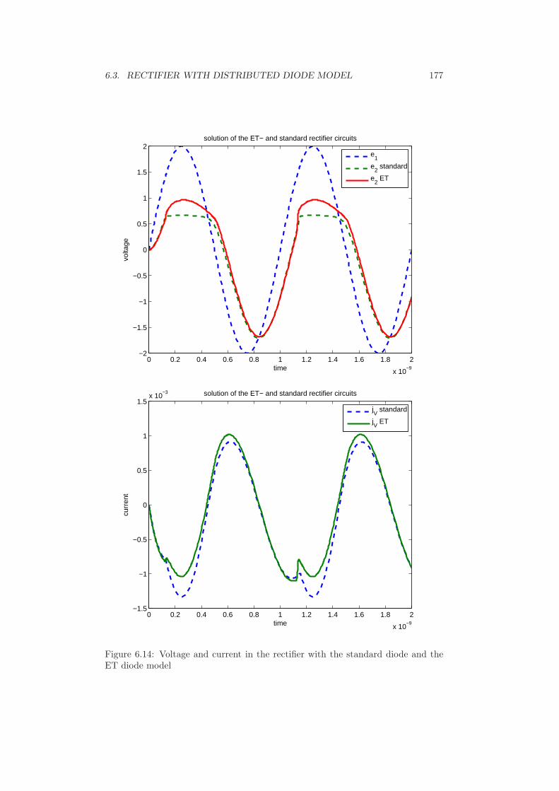
6.3. RECTIFIER WITH DISTRIBUTED DIODE MODEL 177
0 0.2 0.4 0.6 0.8 1 1.2 1.4 1.6 1.8 2
x 10−9
−2
−1.5
−1
−0.5
0
0.5
1
1.5
2
time
volta
ge
solution of the ET− and standard rectifier circuits
e
1
e2 standard
e2 ET
0 0.2 0.4 0.6 0.8 1 1.2 1.4 1.6 1.8 2
x 10−9
−1.5
−1
−0.5
0
0.5
1
1.5x 10
−3
time
curr
ent
solution of the ET− and standard rectifier circuits
jV standard
jV ET
Figure 6.14: Voltage and current in the rectifier with the standard diode and theET diode model

178 CHAPTER 6. NUMERICAL EXAMPLES
6.4 Bridge rectifier with several diodes
A commonly used rectifier circuit is the so-called Graetz-bridge, cf. [101]. It containsfour diodes connected as in Figure 6.15. In comparison to the previously consideredrectifier circuits, this circuit has the advantage that the current is not cut off for thenegative half-wave but reversed. Hence, the Graetz-bridge is a full-wave rectifier.We will study this circuit to investigate the parallelizability of the DI approach forcircuits with several semiconductor devices. The MNA equations for the circuitdepicted in Figure 6.15 are
2CD −CD −CD
−CD 2CD + C −CD − C−CD −CD − C 2CD + C
e1
e2
e3
+
0 0 00 G −G0 −G G
e1
e2
e3
+
1 −1 0 0−1 0 −1 00 1 0 1
g(e1 − e2)g(e3 − e1)
g(e2)g(−e3)
+
100
jV = 0, (6.11a)
e1 = v. (6.11b)
The rectified voltage is measured from node 2 to 3. Here, R = 1G
is the loadresistance and C has been added to flatten the pulsating voltage. The capacitancesCD in parallel to the diodes represent the parasitic capacitance of semiconductorelements. For a simpler representation, these are not depicted in Figure 6.16 butremain in the model of circuit 1. The voltage source v provides a bias voltage as inthe previous example v(t) = 2 sin(2π · 109 · t). We choose R = 103, i.e., G = 10−3.As in the previous section, CD = 10−13 and the flattening capacitance C = 10−11.For the DI simulation, we proceed as in the previous section. We use the lumpeddiode model iD = g(u) to approximate the current that is obtained by solving theET equations of the distributed diode model iD = g(u). The DI equations of thesplit system in Figure 6.16 have the form
2 · 10−13 −10−13 −10−13
−10−13 1.02 · 10−11 −1.01 · 10−11
−10−13 −1.01 · 10−11 1.02 · 10−11
e1
e2
e3
[k]
+
0 0 00 10−3 −10−3
0 −10−3 10−3
e1
e2
e3
[k]
+
1 −1 0 0−1 0 −1 00 1 0 1
g(e[k]1 − e
[k]2 )
g(e[k]3 − e
[k]1 )
g(e[k]2 )
g(−e[k]3 )
+
100
j
[k]V =
j[k−1]K1 − j
′[k−1]K1
j[k−1]K2 − j
′[k−1]K2
j[k−1]K3 − j
′[k−1]K3
,(6.12a)
e[k]1 = v (6.12b)
for system 1 and
1 −1 0 0−1 0 −1 00 1 0 1
g(e′[k]1 − e
′[k]2 )
g(e′[k]3 − e
′[k]1 )
g(−e′[k]2 )
g(e′[k]3 )
+
jK1
jK2
jK3
[k]
= 0, (6.12c)
e′1e′2e′3
[k]
=
e1
e2
e3
[k]
(6.12d)
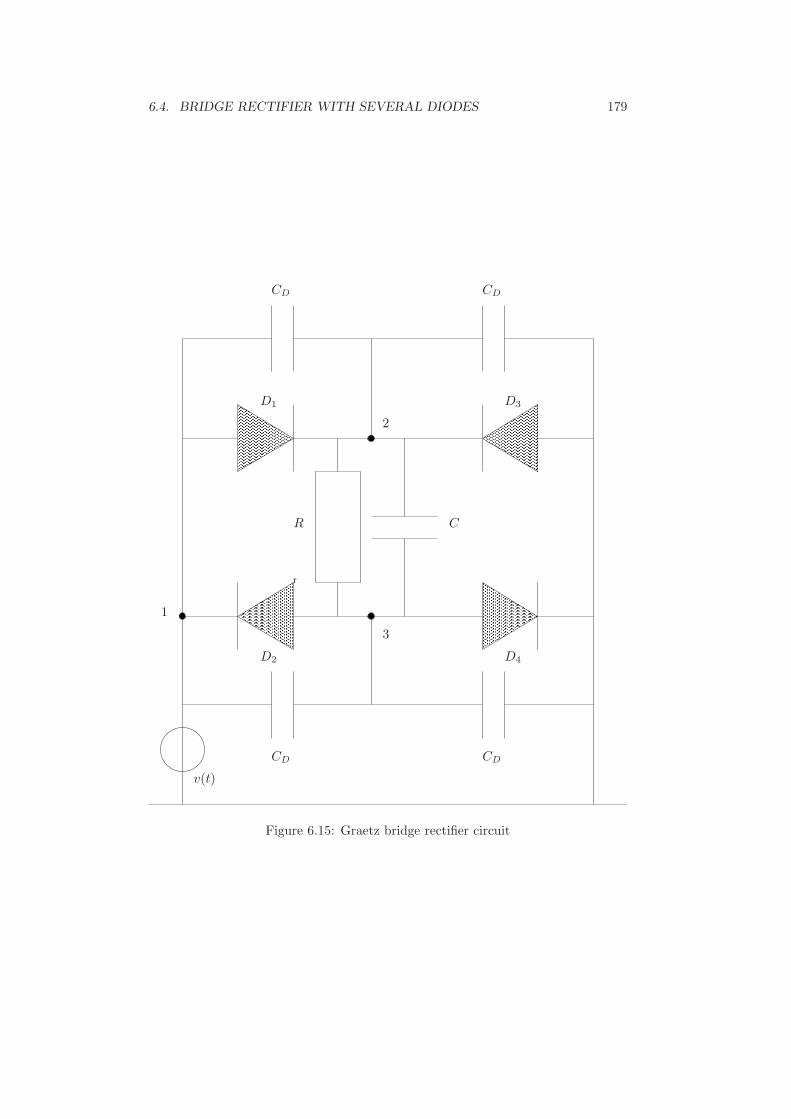
6.4. BRIDGE RECTIFIER WITH SEVERAL DIODES 179
r
1
2
3
C
CD CD
CDCD
R
v(t)
D1
D2
D3
D4
Figure 6.15: Graetz bridge rectifier circuit
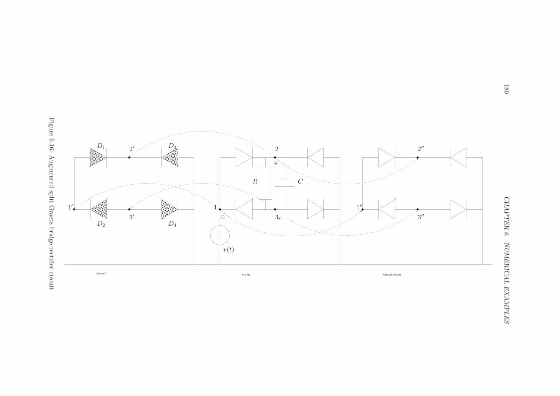
180C
HA
PT
ER
6.
NU
ME
RIC
AL
EX
AM
PLE
S
System 1System 2 Auxiliary System
r r r
1
2
3
1′
2′
3′1′′
2′′
3′′
CR
v(t)
D1
D2
D3
D4
Figu
re6.16:
Augm
ented
split
Graetz
brid
gerectifi
ercircu
it

6.4. BRIDGE RECTIFIER WITH SEVERAL DIODES 181
for system 2. The auxiliary system is given as
1 −1 0 0−1 0 −1 00 1 0 1
g(e′′[k]1 − e
′′[k]2 )
g(e′′[k]3 − e
′′[k]1 )
g(−e′′[k]2 )
g(e′′[k]3 )
+
j′K1
j′K2
j′K3
[k]
= 0, (6.12e)
e′′1e′′2e′′3
[k]
=
e1
e2
e3
[k]
. (6.12f)
System 1 and the auxiliary system can be solved directly by SPICE. If we reformu-late system 2 appropriately, we obtain
j[k]K = −
1 −1 0 0−1 0 −1 00 1 0 1
i[k]D1
i[k]D2
i[k]D3
i[k]D4
, (6.13a)
i[k]D1 = g(e
[k]1 − e
[k]2 ), (6.13b)
i[k]D2 = g(e
[k]3 − e
[k]1 ), (6.13c)
i[k]D3 = g(−e
[k]2 ), (6.13d)
i[k]D4 = g(e
[k]3 ). (6.13e)
In Equations (6.13b-e), we see, that the diode currents are completely independentfrom each other and can be computed with the knowledge of the potentials e1,e2 and e3 which are part of the solution of system 1. This consideration showsan easy way to parallelize the computations within a DI step. As we have seenin the previous section, the most time-consuming computation within one DI stepis the ET diode current. For the current example, four such currents have to becomputed. However, as these computations are completely decoupled, they can beperformed in parallel on different processors. Also, the exchanged data betweenprocessors is only a time-series for the bias voltage at the beginning and anothertime-series for the diode current at the end of computation. No data about thediscretization of the distributed model is exchanged and the communication load iskept low. For the current example, we iterate the DI system (6.12) on the intervalI = [0, 2 · 10−9] with initial values e1(0) = e2(0) = e3(0) = 0, jV (0) = 0 andjK1(0) = jK2(0) = jK3(0) = 0. All starting iterates are constant extrapolationsof these starting values. A parallel implementation of a DI method was not anobjective of this thesis, so we will only show that the concept is working. Equations(6.12c,d) are solved by determining the diode currents sequentially as in Equations(6.13b-e). The coupling currents jK1 to jK3 are computed with (6.13a). Theremaining systems are solved using SPICE. The order of solving the systems is asfollows: first, system 1 is solved, then system 2, then the auxiliary system. Table6.4 shows computation times for 20 DI steps, as well as the difference betweenconsecutive iterates and the rate of convergence. We use the rectified voltage e2−e3
as reference and set
ǫk = ‖e[k]2 − e
[k]3 ‖∞ − ‖e[k−1]
2 − e[k−1]3 ‖∞.
We see that ǫk decreases to about 10−10 within 16 DI steps and then rises to alevel of about 10−6, where it remains more or less constant. These fluctuations maybe explained by errors in the diode current computation which is usually halted ifthe estimated error lies in the magnitude of 10−5. Other reasons for these errors

182 CHAPTER 6. NUMERICAL EXAMPLES
0 0.2 0.4 0.6 0.8 1 1.2 1.4 1.6 1.8 2
x 10−9
−0.1
0
0.1
0.2
0.3
0.4
0.5
0.6
rectified voltage with ET− and standard diode models
time
e 2−e 3
standard diode modelET diode model
Figure 6.17: Rectified voltage with standard and ET diode models
include inaccuracies in the SPICE solutions and due to interpolation as seen in theprevious chapter. However, it can be expected, that the actual error also lies in themagnitude of ǫk which is very satisfactory, given that usually, voltages in SPICEare computed up to an accuracy of 10−3.
The computation times are distinguished between the total of all SPICE calcula-tions, error estimation and administration and the times for the computation ofeach diode current. The total time (sequential) sums up all these contributions.The total (parallel) only adds the time for SPICE and the largest time for a diodecurrent in that step. This gives a good estimate of the time a master process waitsfor all slave processes to finish. The table shows that the major workload in eachDI step is in the computation of the diode currents. If this workload is dividedamong several processes, then the total (estimated) time is reduced significantly. Ifwe assume that the computation is divided among four processors, then the totaltime is reduced to about 25 − 30%, implying almost perfect linear speedup.In Figure 6.17, we see the different solutions for the rectified voltage e2 − e3 usingthe lumped and the ET diode models. The main difference is apparent. With thestandard (lumped) diode model, the voltage across the diode in conducting directiondoes not rise above 0.7. In the bridge circuit in Figure 6.15, two diodes are always inseries with the load and reduce the maximal bias voltage of 2.0 to 2.0− 2 · 0.7 = 0.6which can also be observed in the figure. With the ET diode model, this voltagecut-off happens for much higher bias voltages, e.g., 0.9. What we observe for theGraetz-bridge is that the rectified voltage with the ET diode model is significantlysmaller. With a maximal bias voltage that is smaller than 1.8, we can even expecte2 − e3 to vanish.

6.4
.B
RID
GE
RE
CT
IFIE
RW
ITH
SE
VE
RA
LD
IOD
ES
183
k ǫkǫk
ǫk−1time for SPICE time for iD1 time for iD2 time for iD3 time for iD4 total time (sequential) total time (parallel)
1 3.5 · 10−1 - 1.4s 37.6s 32.0s 32.0s 32.1s 135.1s 39.0s2 1.3 · 10−1 0.38 1.4s 35.5s 40.2s 42.2s 47.9s 167.1s 49.3s3 4.0 · 10−2 0.30 1.5s 46.0s 44.0s 41.2s 33.2s 166.0s 47.5s4 1.0 · 10−2 0.25 1.5s 35.3s 36.2s 35.8s 34.3s 143.1s 37.7s5 1.9 · 10−3 0.19 2.2s 34.4s 35.7s 43.0s 42.3s 157.6s 45.2s6 3.4 · 10−4 0.18 1.9s 42.5s 44.2s 45.0s 44.9s 178.5s 46.9s7 7.1 · 10−5 0.21 2.4s 43.0s 43.3s 42.7s 43.4s 174.8s 45.8s8 5.0 · 10−5 0.70 1.4s 42.0s 36.6s 31.9s 32.1s 144.2s 43.5s9 2.5 · 10−5 0.51 1.7s 32.4s 32.2s 32.9s 32.3s 131.6s 34.6s10 1.4 · 10−5 0.54 1.2s 32.0s 32.3s 32.2s 32.2s 130.0s 33.6s11 4.0 · 10−6 0.29 1.2s 32.2s 32.0s 32.1s 32.4s 130.0s 33.6s12 7.7 · 10−7 0.19 1.2s 32.0s 31.9s 31.9s 32.4s 129.5s 33.7s13 2.2 · 10−7 0.28 1.4s 32.2s 32.0s 32.3s 32.3s 130.3s 33.7s14 2.8 · 10−8 0.13 1.2s 32.2s 32.2s 32.0s 32.3s 129.9s 33.5s15 3.0 · 10−9 0.11 1.4s 32.5s 31.6s 31.6s 32.0s 129.2s 34.0s16 3.8 · 10−10 0.13 1.2s 31.9s 31.6s 31.8s 32.2s 128.7s 33.4s17 1.0 · 10−7 265.2 1.2s 31.8s 31.9s 31.6s 31.9s 128.4s 33.0s18 1.3 · 10−7 1.3 1.2s 31.9s 31.5s 31.8s 31.9s 128.4s 33.2s19 3.3 · 10−6 25.4 1.2s 31.9s 31.7s 32.1s 32.1s 129.0s 33.3s20 2.3 · 10−6 0.68 1.2s 31.6s 31.5s 31.6s 31.8s 127.9s 33.0s
Table 6.4: Simulation results for Graetz-bridge rectifier

184 CHAPTER 6. NUMERICAL EXAMPLES
6.5 Conclusion
In this chapter we have considered a series of related examples. We have demon-strated that dynamic iteration is a viable approach for the simulation of electricalcircuits. We have shown that the concepts of convergence acceleration and macrostep size control are efficient and realizable using standard simulation software suchas SPICE. None of the simulations with split systems were competitive with SPICEsimulations of the full system. However, the potential of dynamic iteration methodswas demonstrated for two simulator coupling problems. The DI approach allowedthe simulation of circuits with incompatible simulation tools. With Matlab as aninterface, it was possible to do SPICE simulations with diode models that do nothave equivalent representations in the SPICE environment. For the standard rec-tifier and the Graetz-bridge, we have compared the results using different diodemodels and obtained significantly different results. These examples not only provethe feasibility of the DI process for circuits with distributed elements but also show,why non-standard semiconductor models need to be considered in some cases.
Chapter 7
Summary
The purpose of this thesis was the analysis of partitioned simulation of electricalcircuits. Special emphasis has been put on two points. First, the analytical resultsshould have graph theoretical interpretations. This requirement is based on thefact that the differential-algebraic equations arising in circuit simulation are oftenvery large and badly scaled and do not allow an analysis with standard tools fromlinear algebra, such as SVD. And secondly, all developed methods shall work withstandard circuit simulation tools, such that these methods can easily be includedinto existing software. The widely used circuit simulation tool SPICE and the cor-responding netlist format have been used as reference.Some basic concepts from analysis and linear algebra, together with a brief intro-duction into the theory of DAEs, graph theory and circuit simulation were given inChapter 2. The method of choice for the setup of circuit equations was the ModifiedNodal Analysis. We have also presented concepts of expressing range, kernel andrank of circuit related matrices with the help of graph structures such as loops andcutsets.In Chapter 3, we have reviewed the basic concepts of Dynamic Iteration methodsfor the solution of partitioned ODEs and DAEs. For these two types of dynamic sys-tems, the convergence behaviour of the Dynamic Iteration process is fundamentallydifferent. Sufficient criteria for convergence have been presented. While for ODEs,under very weak assumptions, rapid convergence of the method can always be ex-pected, the convergence behaviour of Dynamic Iteration for DAEs depends on thespectral properties of a problem specific matrix. If this matrix has a spectral radiusof zero, then the Dynamic Iteration method for the DAE behaves as in the ODEcase, i.e., convergence is fast and guaranteed. This type of convergence behaviourhas been called quasi-instantaneous. For nonvanishing spectral radii, convergencedepends on whether this spectral radius is smaller or larger than one. This kindof convergence behaviour is already known from matrix iteration schemes for linearsystems. Convergence or divergence in this case is linear at best and related tothe underlying algebraic iteration method. We have mainly restricted our consid-erations to Dynamic Iteration methods for DAEs of differentiation index one thatare coupled in a special way. In the more general case, another type of iterationbehaviour may occur where, usually, the iterates diverge rapidly. This is the casewhen a problem related pencil has eigenvalues at infinity. The block Jacobi andblock Gauss-Seidel methods, which are well-known from matrix iterative analysiscan easily be extended to the problem of Dynamic Iteration for coupled systemsof semi-explicit DAEs. In this case, the convergence criterion becomes easier tocheck. Also, some approaches for a modified Dynamic Iteration method to guaran-tee convergence for semi-explicit DAEs with the block Jacobi and block Gauss-Seidelmethods have been proposed. It has been shown, that with these modifications, it
185

186 CHAPTER 7. SUMMARY
is even possible to attain quasi-instantaneous convergence behaviour.In Chapter 4, these results were applied to the task of partitioned circuit simu-lation. We have first presented an overlap-free splitting technique that allows aninterpretation of the split circuit equations as circuit netlist. This feature is essen-tial for the compatibility with existing circuit simulation software. The overlap-freesplitting allows to isolate single circuit elements and to simulate them separately.For the analysis of Dynamic Iteration methods for circuits, we only allow resistive,capacitive and inductive elements as well as independent sources. This restrictionwas necessary for a concise characterization of convergence behaviour. We havefirst investigated the convergence behaviour for purely resistive circuits and shownhow the freedom in the splitting of the circuit influences the speed of convergence.However, it was not possible to construct a convergent method for all cases in thisway. We have then extended the obtained results to RCL circuits. It was possi-ble to show that these circuits can be analyzed using the results from the resistivecase for three specially constructed subcircuits of the RCL circuit. The results forresistive circuits then carry over to the more general RCL case. The problem ofnonconvergence was addressed in Section 4.4, where methods have been developedthat force or accelerate convergence of the Dynamic Iteration method by extendingcertain parts of the circuit. This has been investigated in detail for purely resistivecircuits and then extended to the more general RCL case. Again, the approach al-lows an interpretation in terms of circuit modifications as a means of manipulatingthe circuit equations.The more numerical aspects of Dynamic Iteration were investigated in Chapter 5.For the previous results, it has been assumed that all equations were exactly solv-able. In this chapter, we take errors from numerical integration and interpolationof previous solutions into account. We were able to state a convergence result forDynamic Iteration methods that include these errors. Furthermore, we have inves-tigated the influence of macro step sizes on work load and approximation errors anddevised a simple but functional macro step size controller.The obtained results have been validated in Chapter 6 with the help of four ex-amples. The used circuit simulation software is the freely available code SPICE.The convergence acceleration method and the macro step size controller have beentested in Section 6.1 for a simple rectifier circuit. In Section 6.2, a linearized modelof the rectifier, where an explicit solution is available, is used to show that pre-scribed accuracy requirements are met. In Section 6.3, we have used a PDE modelfor the diode in the rectifier. The PDE is treated by a specialized solver whilethe remainder of the circuit is simulated in SPICE. The coupling between the twosimulators is done via the Dynamic Iteration method. In Section 6.4, this exampleis extended to a circuit with four diodes that are solved separately. In this section,we show the possibility of parallelizing the Dynamic Iteration approach in a verysimple but effective way.Concluding, we have shown that the Dynamic Iteration approach is an easy andeffective way to simulate different parts of a circuit using different solvers. Thismay be less efficient than a SPICE simulation of the full circuit. However, in caseswhere this is not possible, e.g., for the simulation of circuits with PDE device mod-els, Dynamic Iteration becomes very efficient and is easily implemented into existingsimulation software environments.
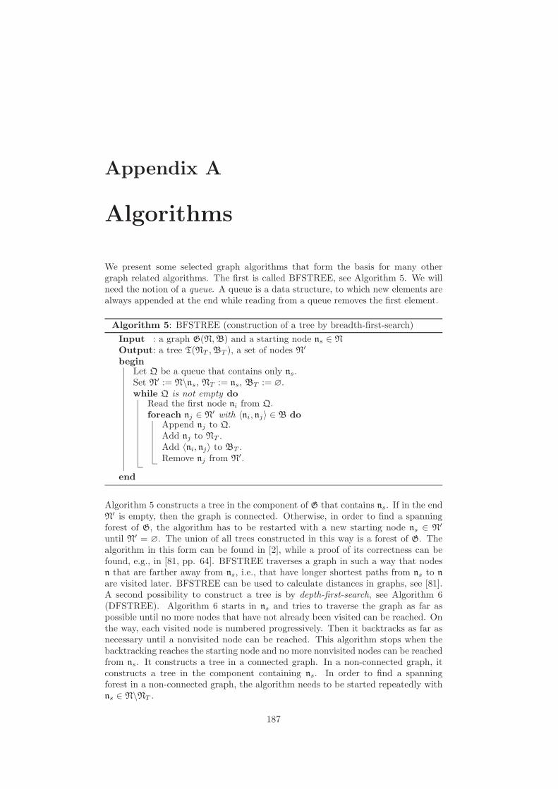
Appendix A
Algorithms
We present some selected graph algorithms that form the basis for many othergraph related algorithms. The first is called BFSTREE, see Algorithm 5. We willneed the notion of a queue. A queue is a data structure, to which new elements arealways appended at the end while reading from a queue removes the first element.
Algorithm 5: BFSTREE (construction of a tree by breadth-first-search)
Input : a graph G(N, B) and a starting node ns ∈ N
Output: a tree T(NT , BT ), a set of nodes N′
beginLet Q be a queue that contains only ns.Set N′ := N\ns, NT := ns, BT := ∅.while Q is not empty do
Read the first node ni from Q.foreach nj ∈ N′ with 〈ni, nj〉 ∈ B do
Append nj to Q.Add nj to NT .Add 〈ni, nj〉 to BT .Remove nj from N′.
end
Algorithm 5 constructs a tree in the component of G that contains ns. If in the endN′ is empty, then the graph is connected. Otherwise, in order to find a spanningforest of G, the algorithm has to be restarted with a new starting node ns ∈ N′
until N′ = ∅. The union of all trees constructed in this way is a forest of G. Thealgorithm in this form can be found in [2], while a proof of its correctness can befound, e.g., in [81, pp. 64]. BFSTREE traverses a graph in such a way that nodesn that are farther away from ns, i.e., that have longer shortest paths from ns to n
are visited later. BFSTREE can be used to calculate distances in graphs, see [81].A second possibility to construct a tree is by depth-first-search, see Algorithm 6(DFSTREE). Algorithm 6 starts in ns and tries to traverse the graph as far aspossible until no more nodes that have not already been visited can be reached. Onthe way, each visited node is numbered progressively. Then it backtracks as far asnecessary until a nonvisited node can be reached. This algorithm stops when thebacktracking reaches the starting node and no more nonvisited nodes can be reachedfrom ns. It constructs a tree in a connected graph. In a non-connected graph, itconstructs a tree in the component containing ns. In order to find a spanningforest in a non-connected graph, the algorithm needs to be started repeatedly withns ∈ N\NT .
187

188 APPENDIX A. ALGORITHMS
Algorithm 6: DFSTREE (construction of a tree by depth-first-search)
Input : a graph G(N, B) and a starting node ns ∈ N
Output: a tree T(NT , BT ), a node-valued predecessor function nj = p(ni)and a numbering of nodes nr(ni) for all ni ∈ N
beginSet NT := ns, BT := ∅.Set B′ := ∅.foreach ni ∈ N do
Set nr(ni) := 0.Set p(ni) := 0.
Set ni := ns, k := 1, nr(ni) := k.repeat
while there exists nj ∈ N with 〈ni, nj〉 ∈ B but 〈ni, nj〉 /∈ B′ doChoose one nj ∈ N with 〈ni, nj〉 ∈ B but 〈ni, nj〉 /∈ B′.Add 〈ni, nj〉 to B′.if nr(nj) = 0 then
Add nj to NT .Add 〈ni, nj〉 to BT .Set k := k + 1.Set nr(nj) := k.Set p(nj) := ni.Set ni = nj .
Set ni := p(ni).until ni = ns and all 〈ni, nj〉 ∈ B′ if 〈ni, nj〉 ∈ B
end
The numbering nr is not necessary but helpful for Algorithm 7 (BLOCKCUT)which is an extension of DFSTREE that identifies all blocks of a given graph. Inaddition to this numbering, BLOCKCUT calculates the lowpoint function low(n)for each node, cf. [2]. This function is the lowest nr(·) of any node that lies in afundamental loop, with n. This information is then used to determine all blocksof a given undirected graph. For simplicity, we assume that G(N, B) is connected.Furthermore, we will use the notion of a stack. A stack is a data structure, wherenew data is appended at the end, but unlike the queue, reading from the stackremoves the last element.BLOCKCUT determines the nodesets Nl of all blocks of a graph G(N, B). Theblocks are then given as the induced subgraphs GB,l(NB,l, B|NB,l), wherel = 1, . . . , |NA| − 1. The correctness of Algorithm 7 is proved, e.g., in [2, 81].

189
Algorithm 7: BLOCKCUT (determination of then nodesets of all blocks)
Input : an undirected, connected graph G(N, B) and a starting nodens ∈ N
Output: a set NA of articulation points, nodesets NB,l, l = 1, . . . , (|NA| − 1)of all blocks of G
beginSet NT := ns, BT := ∅.Set B′ := ∅.Set NA := ∅.foreach ni ∈ N do
Set nr(ni) := 0.Set p(ni) := 0.
Set ni := ns, k := 1, nr(ni) := 1, l := 0, low(ns) = 1.Let S be a stack that contains only ns.repeat
while there exists nj ∈ N with 〈ni, nj〉 ∈ B but 〈ni, nj〉 /∈ B′ doChoose one nj ∈ N with 〈ni, nj〉 ∈ B but 〈ni, nj〉 /∈ B′.Add 〈ni, nj〉 to B′.if nr(nj) = 0 then
Add nj to S.Set k := k + 1.Set nr(nj) := k.Set low(nj) := k.Set p(nj) := ni
Set ni = nj .
elseSet low(ni) = min(low(ni), nr(p(nj))).
if p(ni) 6= ns thenif low(ni) < nr(p(ni)) then
Set low(p(ni)) = min(low(ni), low(p(ni))).
elseAdd p(ni) to NA. Set l := l + 1.Remove nodes from S and add them to NB,l until ni isremoved.Add p(ni) to NB,l.
elseif there exists nj ∈ N with 〈ns, nj〉 ∈ B but 〈ns, nj〉 /∈ B′ then
Add ns to NA.Set l := l + 1.Remove nodes from S and add them to NB,l until ni is removed.Add ns to NB,l.
Set ni := p(ni).until ni = ns and B′ = B
end

190 APPENDIX A. ALGORITHMS

Appendix B
Index conditions for
controlled sources
In the following, we present conditions for controlled sources in lumped circuitsthat guarantee that the d-index of the circuit DAE is not larger than 2. They canoriginally be found in [43] or [45]. The presented tables are taken from [12].
Controlled voltage sources
The controlled voltage sources are not allowed to be part of CV loops. The con-trolling elements have to fulfill the conditions given in Table B.1 for voltage con-trolled voltage sources (VCVS) and Table B.2 for current controlled voltage sources(CCVS).
The controlling voltage of a VCVS can be the voltages across
1. capacitances,
2. independent voltage sources,
3. CCVSs that are controlled by the currents through
(a) inductances,
(b) independent current sources,
(c) resistances or VCCSs for which the nodes that are incident withthe controlling branch are connected by
i. capacitances,
ii. independent voltage sources,
iii. paths that contain only elements that are described in (3(c)i)and (3(c)ii),
(d) branches that form a cutset with elements described in (3a), (3b)and (3c),
4. branches that form a loop with elements described in (1), (2) and (3).
Table B.1: Conditions for VCVS
191
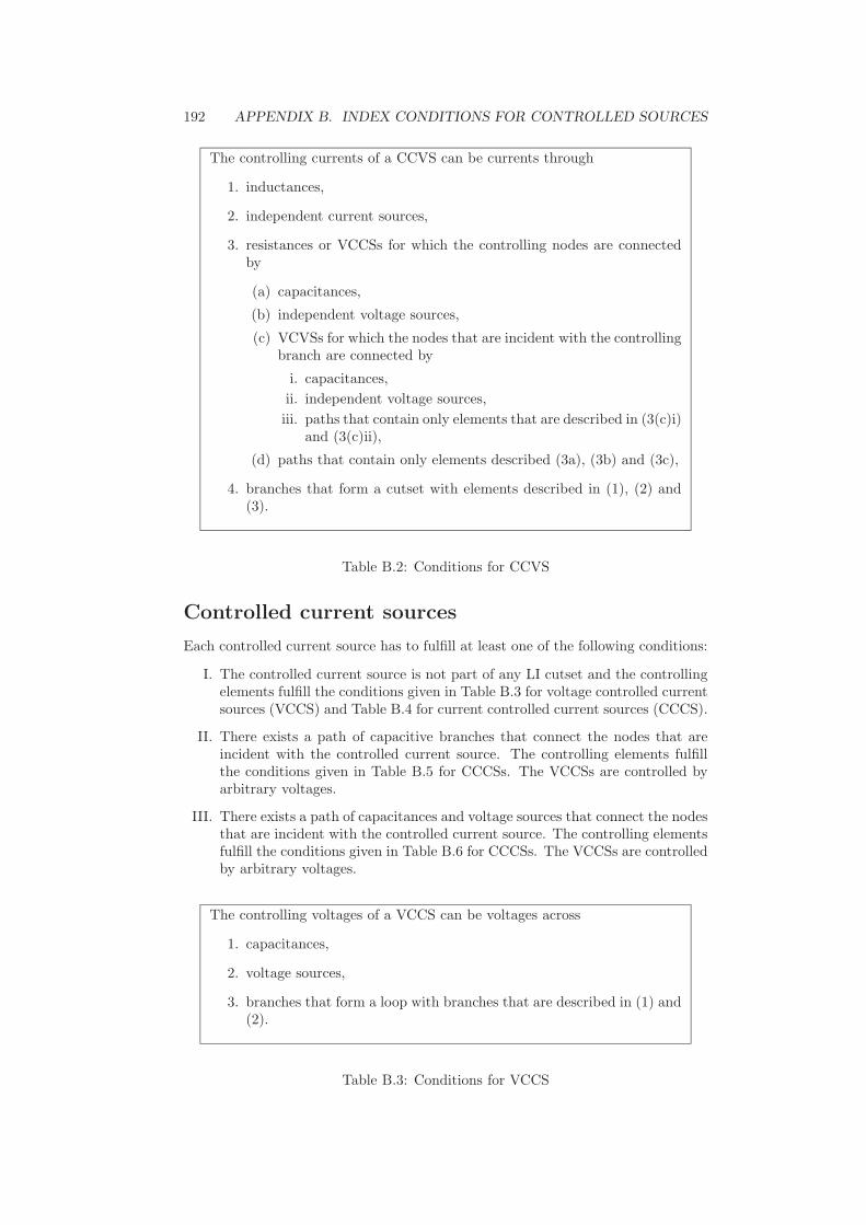
192 APPENDIX B. INDEX CONDITIONS FOR CONTROLLED SOURCES
The controlling currents of a CCVS can be currents through
1. inductances,
2. independent current sources,
3. resistances or VCCSs for which the controlling nodes are connectedby
(a) capacitances,
(b) independent voltage sources,
(c) VCVSs for which the nodes that are incident with the controllingbranch are connected by
i. capacitances,
ii. independent voltage sources,
iii. paths that contain only elements that are described in (3(c)i)and (3(c)ii),
(d) paths that contain only elements described (3a), (3b) and (3c),
4. branches that form a cutset with elements described in (1), (2) and(3).
Table B.2: Conditions for CCVS
Controlled current sources
Each controlled current source has to fulfill at least one of the following conditions:
I. The controlled current source is not part of any LI cutset and the controllingelements fulfill the conditions given in Table B.3 for voltage controlled currentsources (VCCS) and Table B.4 for current controlled current sources (CCCS).
II. There exists a path of capacitive branches that connect the nodes that areincident with the controlled current source. The controlling elements fulfillthe conditions given in Table B.5 for CCCSs. The VCCSs are controlled byarbitrary voltages.
III. There exists a path of capacitances and voltage sources that connect the nodesthat are incident with the controlled current source. The controlling elementsfulfill the conditions given in Table B.6 for CCCSs. The VCCSs are controlledby arbitrary voltages.
The controlling voltages of a VCCS can be voltages across
1. capacitances,
2. voltage sources,
3. branches that form a loop with branches that are described in (1) and(2).
Table B.3: Conditions for VCCS

193
The controlling current of a CCCS can be the current through
1. inductances,
2. independent current sources,
3. resistances or VCCSs for which the nodes that are incident with theCCCS are connected by
(a) capacitances,
(b) voltage sources,
(c) paths that contain only elements described in (3a) and (3b),
4. branches that form a cutset with elements described in (1), (2) and(3).
Table B.4: Conditions for CCCS in case I.
The controlling current of a CCCS can be the current through
1. inductances,
2. independent current sources,
3. resistances,
4. voltage sources that do not belong to any CV loops,
5. VCCSs,
6. a branch that forms a cutset with elements described in (1) – (5).
Table B.5: Conditions for CCCS in case II.
The controlling current of a CCCS can be the current through
1. inductances,
2. resistances,
3. independent current sources,
4. VCCSs,
5. a branch that forms a cutset with elements described in (1) – (4).
Table B.6: Conditions for CCCS in case III.

194 APPENDIX B. INDEX CONDITIONS FOR CONTROLLED SOURCES

Appendix C
The SPICE circuit simulator
In this section, we will give a brief overview on the SPICE circuit simulator. TheSimulation Program with Integrated Circuit Emphasis (SPICE) was first presentedin 1973. Two years later, SPICE2 followed which already contained much of thefunctionality of current SPICE versions and derivates. Many of today’s circuitsimulation tools are more or less based on these early programs, e.g., HSPICE(Synopsis), PSPICE (Cadence Design Systems), Cider (UC Berkeley/Oregon StateUniversity), TISPICE (Texas Instruments) or PowerSpice (IBM) to name only afew. Starting with SPICE2, the program took a text file called netlist as input andproduced printer listings as output. With SPICE3, graphical output functionalitywas added and several graphical user interfaces were developed for SPICE, withPSPICE probaly being the most commonly used today.We will subseqently present some typical elements of SPICE netlists where we con-centrate on those elements that are used in this thesis. In-depth descriptions ofnetlist syntax and circuit elements may be found in [84,86,111,112] or online at [1].
C.1 Circuit elements
The SPICE circuit simulator offers a wide range of circuit elements to be simulated.We will present only the most basic elements, i.e., those presented in Section 2.5.
C.1.1 Linear two-term elements
The notation of a linear resistor, a linear capacitor and a linear inductor in a netlistare the following
RXXXXXXX N1 N2 VALUE
CXXXXXXX N1 N2 VALUE
LXXXXXXX N1 N2 VALUE
where XXXXXXX is an arbitrary alphanumerical string. The entries N1 and N2 are thenames of the two terminal nodes of the resistor and VALUE is the resistance/ capac-itance/ inductance value of the element in Ohms/ Farads/ Henries, respectively.
C.1.2 Semiconductor diodes
The only semiconductor element used in this thesis is a diode. The netlist repre-sentation as used in the thesis is the following
DXXXXXXX N1 N2 MNAME.
195

196 APPENDIX C. THE SPICE CIRCUIT SIMULATOR
parameter explanation
IS saturation current [A]RS ohmic resistance [Ω]N emission coefficientTT transit time [s]CJO zero-bias junction capacitance [F ]VJ junction potential [V ]EG activation energy [eV ]BV reverse breakdown voltage [V ]
TNOM parameter measurement temperature [C]
Table C.1: Parameters for diode models
The standard definition allows for additional parameters to be specified such asdevice temperature. The string XXXXXXX carries the unique name of the elementand N1 and N2 are the terminal nodes of the diode. Note that the diode is an ori-ented element and that it is considered in conducting direction for positive voltagesfrom N1 to N2 and in reverse biasing for negative voltages from N1 to N2. The al-phanumeric string MNAME specifies the used diode parameters. These have to be setusing the command
.MODEL MNAME TYPE(PNAME1=PVAL1 PNAME2=PVAL2 ... ).
Here, MNAME specifies the name of the parameter setting. TYPE is the type ofelement for which parameters are set, e.g., D for diodes, NPN/PNP for NPN/PNPbipolar junction transistors, NMOS/PMOS for N-channel/P-channel MOSFET modelsetc. The pair PNAMEi=PVALi sets one specific parameter for the MNAME model. Typ-ical diode parameters are listed in Table C.1. This list is incomplete. A full list isfound, e.g., in [84]. The diode current iD is computed by the function
iD = IS(exp(u
VT
) − 1) (C.1)
where IS is specified by IS, u is the applied voltage from N1 to N2 and
VT =NKT
qe
.
Here, N is the emission coeficient as specified by N, K is Boltzman’s constant(K = 1.3806503 · 1023m2kgs−2K−1), T is the absolute temperature of the deviceand qe is the elementary charge of the electron (qe = 1.60217646 ·10−19C). Differentversions of equation (C.1) are used for different operating regions of the diode.Additional properties such as the ohmic resistance of the element are modeled byan additional ohmic resistor and the junction capacitance is modelled by a parallelcapacitance. For more information on semiconductor models, we refer to [84].
C.1.3 Independent sources
We will only present some sources that were used to model the examples in Chap-ter 6. The notation of independent voltage- and current sources is the following
VXXXXXXX N+ N- <TYPE> <(PVAL1 PVAL2 ... )>
IXXXXXXX N+ N- <TYPE> <(PVAL1 PVAL2 ... )>
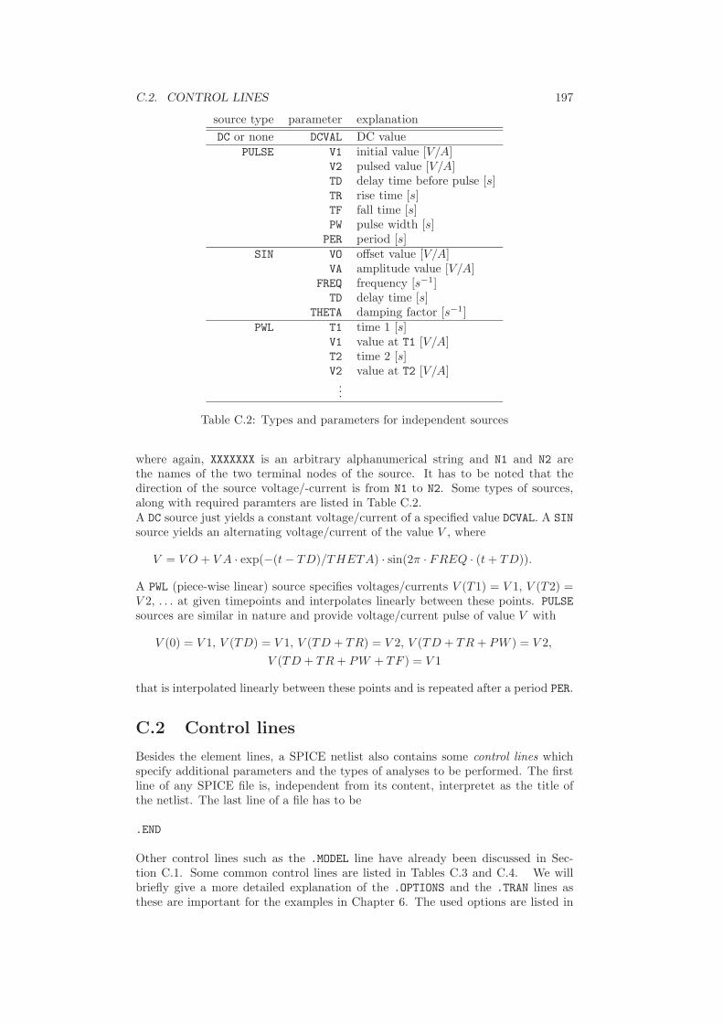
C.2. CONTROL LINES 197
source type parameter explanation
DC or none DCVAL DC valuePULSE V1 initial value [V/A]
V2 pulsed value [V/A]TD delay time before pulse [s]TR rise time [s]TF fall time [s]PW pulse width [s]PER period [s]
SIN VO offset value [V/A]VA amplitude value [V/A]
FREQ frequency [s−1]TD delay time [s]
THETA damping factor [s−1]PWL T1 time 1 [s]
V1 value at T1 [V/A]T2 time 2 [s]V2 value at T2 [V/A]
...
Table C.2: Types and parameters for independent sources
where again, XXXXXXX is an arbitrary alphanumerical string and N1 and N2 arethe names of the two terminal nodes of the source. It has to be noted that thedirection of the source voltage/-current is from N1 to N2. Some types of sources,along with required paramters are listed in Table C.2.A DC source just yields a constant voltage/current of a specified value DCVAL. A SIN
source yields an alternating voltage/current of the value V , where
V = V O + V A · exp(−(t − TD)/THETA) · sin(2π · FREQ · (t + TD)).
A PWL (piece-wise linear) source specifies voltages/currents V (T1) = V 1, V (T2) =V 2, . . . at given timepoints and interpolates linearly between these points. PULSE
sources are similar in nature and provide voltage/current pulse of value V with
V (0) = V 1, V (TD) = V 1, V (TD + TR) = V 2, V (TD + TR + PW ) = V 2,
V (TD + TR + PW + TF ) = V 1
that is interpolated linearly between these points and is repeated after a period PER.
C.2 Control lines
Besides the element lines, a SPICE netlist also contains some control lines whichspecify additional parameters and the types of analyses to be performed. The firstline of any SPICE file is, independent from its content, interpretet as the title ofthe netlist. The last line of a file has to be
.END
Other control lines such as the .MODEL line have already been discussed in Sec-tion C.1. Some common control lines are listed in Tables C.3 and C.4. We willbriefly give a more detailed explanation of the .OPTIONS and the .TRAN lines asthese are important for the examples in Chapter 6. The used options are listed in

198 APPENDIX C. THE SPICE CIRCUIT SIMULATOR
control line parameters explanation
.SUBCKT subnam N1 <N2 N3 ...> beginning of a subcircuit definition.ENDS - end of a subcircuit definition
.INCLUDE filename includes filename
.NODESET V(NODE)=VAL initial guess of voltage at NODE.IC V(NODE)=VAL initial condition for voltage at NODE
.OPTIONS OPT=OPTVAL sets option OPT to OPTVAL
Table C.3: Non-analysis control lines
control line explanation
.DC DC-sweep analysis
.AC AC small-signal analysis
.TF transfer function analysis
.PZ pole-zero analysis.SENS sensitivity analysis.DISTO distortion analysis
.OP DC operation point analysis.TRAN transient analysis
Table C.4: Types of circuit analysis
Table C.5. The options METHOD = TRAPEZOIDAL specifies the use of the trapezoidalrule, see Table 5.3. The choice METHOD = GEAR switches to the BDF method, seeTable 5.1. The order of the used BDF method is chosen automatically but limitedby the number specified with MAXORD.All SPICE examples in Chapter 6 were transient analyses. The general form of the.TRAN line is
.TRAN TSTEP TSTOP [ [ TSTART ] TMAX ].
The parameter TSTEP is the suggested initial stepsize of the integration methodand TMAX the maximal allowed stepsize. The latter can be used to force SPICE toproduce a sufficiently dense output such that interpolation of the output yields onlysmall errors. TSTOP specifies the end of the computation interval. The parameterTSTART marks the beginning of the interval, where output is generated. All tran-sient simulations start at time 0 and also initial conditions may only be prescribedat time 0. In order to perform simulations on different intervals, it is a good solutionto shift the independent sources in time. The bias voltage of the simple rectifier inChapter 6 was specified with the line
VIN 1 0 SIN 0 5 1 $t start
where $tstart was replaced by the desired t0 with the help of a Perl script priorto the SPICE call.
option explanation
ABSTOL=x sets the absolute current error tolerance to x[A] (default 10−12A)VNTOL=x sets the absolute voltage error tolerance to x[V] (default 10−6V )RELTOL=x sets the relative error tolerance to x (default 10−3)
METHOD=name numerical integration method TRAPEZOIDAL(default) or GEARMAXORD=x sets the maximal order of the BDF (GEAR) method (default 2)
Table C.5: Parameters for .OPTIONS

List of Figures
2.1 common load elements (from left to right): ideal resistor, diode, idealcapacitor, ideal inductor . . . . . . . . . . . . . . . . . . . . . . . . . 30
2.2 common types of sources (from left to right): independent voltagesource, controlled voltage source, independent current source, con-trolled current source . . . . . . . . . . . . . . . . . . . . . . . . . . . 31
2.3 n-term element . . . . . . . . . . . . . . . . . . . . . . . . . . . . . . 32
3.1 Schematic representation of the Jacobi (left) and Gauss-Seidel-DIM(right) for two systems . . . . . . . . . . . . . . . . . . . . . . . . . . 54
4.1 Splitting of a circuit (above) across a branch into two subcircuits(below) . . . . . . . . . . . . . . . . . . . . . . . . . . . . . . . . . . 76
4.2 MOS transistor . . . . . . . . . . . . . . . . . . . . . . . . . . . . . . 764.3 node with incident branches (left), duplicated nodes with distributed
branches (right) . . . . . . . . . . . . . . . . . . . . . . . . . . . . . . 814.4 coupling source pair . . . . . . . . . . . . . . . . . . . . . . . . . . . 814.5 left: original circuit, center: pre-splitting circuit, right: split circuit . 824.6 two consistent source assignments for one splitting node together
with their graphical representation . . . . . . . . . . . . . . . . . . . 844.7 relevant and non-relevant branches and nodes . . . . . . . . . . . . . 924.8 original circuit, (a-d) split circuit with possible source assignments . 994.9 example RCL circuit . . . . . . . . . . . . . . . . . . . . . . . . . . . 1044.10 C-, G- and L-subcircuits . . . . . . . . . . . . . . . . . . . . . . . . . 1044.11 simple RCL circuit . . . . . . . . . . . . . . . . . . . . . . . . . . . . 1214.12 left: pre-splitting C-subcircuit, right: split C-subcircuit . . . . . . . 1214.13 left: pre-splitting G-subcircuit, right: split G-subcircuit . . . . . . . 1214.14 Example circuit in original (left) and split (right) form. . . . . . . . 132
4.15 C-subcircuit (left) and G-subcircuit (right). . . . . . . . . . . . . . . 1324.16 Augmented example circuit. . . . . . . . . . . . . . . . . . . . . . . . 1344.17 Two connected capacitances (a) and the two capacitances in different
subcircuits (b). . . . . . . . . . . . . . . . . . . . . . . . . . . . . . . 1364.18 Two connected inductances (a) and the two inductances in different
subcircuits (b). . . . . . . . . . . . . . . . . . . . . . . . . . . . . . . 1364.19 Connected conductance and capacitance (a), both elements in differ-
ent subcircuits (b), split C-subcircuit (c). . . . . . . . . . . . . . . . 137
5.1 PWL voltage source . . . . . . . . . . . . . . . . . . . . . . . . . . . 1445.2 Approximation of the integral by lower sums . . . . . . . . . . . . . 1525.3 The first iterates and errors for the DIM (5.31) . . . . . . . . . . . . 1545.4 The first iterates and errors for the DIM (5.31) with two macro steps 155
6.1 Simple rectifier circuit (left), split rectifier circuit (right) . . . . . . . 162
199
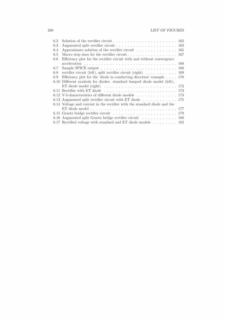
200 LIST OF FIGURES
6.2 Solution of the rectifier circuit . . . . . . . . . . . . . . . . . . . . . . 1626.3 Augmented split rectifier circuit . . . . . . . . . . . . . . . . . . . . . 1636.4 Approximate solution of the rectifier circuit . . . . . . . . . . . . . . 1656.5 Macro step sizes for the rectifier circuit . . . . . . . . . . . . . . . . . 1676.6 Efficiency plot for the rectifier circuit with and without convergence
acceleration . . . . . . . . . . . . . . . . . . . . . . . . . . . . . . . . 1686.7 Sample SPICE output . . . . . . . . . . . . . . . . . . . . . . . . . . 1686.8 rectifier circuit (left), split rectifier circuit (right) . . . . . . . . . . . 1696.9 Efficiency plot for the ’diode in conducting direction’ example . . . . 1706.10 Different symbols for diodes: standard lumped diode model (left),
ET diode model (right) . . . . . . . . . . . . . . . . . . . . . . . . . 1726.11 Rectifier with ET diode . . . . . . . . . . . . . . . . . . . . . . . . . 1736.12 V-I-characteristics of different diode models . . . . . . . . . . . . . . 1736.13 Augmented split rectifier circuit with ET diode . . . . . . . . . . . . 1756.14 Voltage and current in the rectifier with the standard diode and the
ET diode model . . . . . . . . . . . . . . . . . . . . . . . . . . . . . . 1776.15 Graetz bridge rectifier circuit . . . . . . . . . . . . . . . . . . . . . . 1796.16 Augmented split Graetz bridge rectifier circuit . . . . . . . . . . . . 1806.17 Rectified voltage with standard and ET diode models . . . . . . . . 182
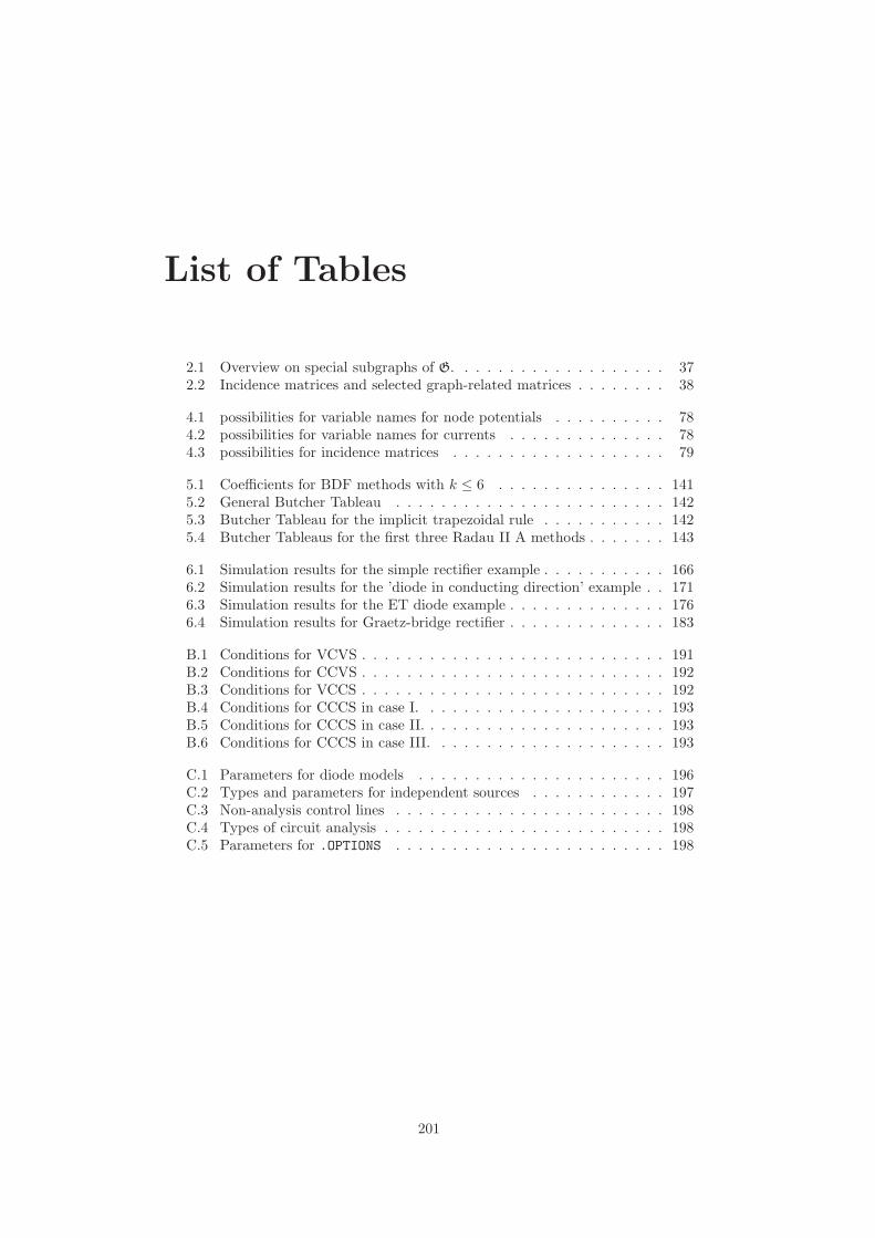
List of Tables
2.1 Overview on special subgraphs of G. . . . . . . . . . . . . . . . . . . 372.2 Incidence matrices and selected graph-related matrices . . . . . . . . 38
4.1 possibilities for variable names for node potentials . . . . . . . . . . 784.2 possibilities for variable names for currents . . . . . . . . . . . . . . 784.3 possibilities for incidence matrices . . . . . . . . . . . . . . . . . . . 79
5.1 Coefficients for BDF methods with k ≤ 6 . . . . . . . . . . . . . . . 1415.2 General Butcher Tableau . . . . . . . . . . . . . . . . . . . . . . . . 1425.3 Butcher Tableau for the implicit trapezoidal rule . . . . . . . . . . . 1425.4 Butcher Tableaus for the first three Radau II A methods . . . . . . . 143
6.1 Simulation results for the simple rectifier example . . . . . . . . . . . 1666.2 Simulation results for the ’diode in conducting direction’ example . . 1716.3 Simulation results for the ET diode example . . . . . . . . . . . . . . 1766.4 Simulation results for Graetz-bridge rectifier . . . . . . . . . . . . . . 183
B.1 Conditions for VCVS . . . . . . . . . . . . . . . . . . . . . . . . . . . 191B.2 Conditions for CCVS . . . . . . . . . . . . . . . . . . . . . . . . . . . 192B.3 Conditions for VCCS . . . . . . . . . . . . . . . . . . . . . . . . . . . 192B.4 Conditions for CCCS in case I. . . . . . . . . . . . . . . . . . . . . . 193B.5 Conditions for CCCS in case II. . . . . . . . . . . . . . . . . . . . . . 193B.6 Conditions for CCCS in case III. . . . . . . . . . . . . . . . . . . . . 193
C.1 Parameters for diode models . . . . . . . . . . . . . . . . . . . . . . 196C.2 Types and parameters for independent sources . . . . . . . . . . . . 197C.3 Non-analysis control lines . . . . . . . . . . . . . . . . . . . . . . . . 198C.4 Types of circuit analysis . . . . . . . . . . . . . . . . . . . . . . . . . 198C.5 Parameters for .OPTIONS . . . . . . . . . . . . . . . . . . . . . . . . 198
201

202 LIST OF TABLES

List of Algorithms
1 Coupling source assignment . . . . . . . . . . . . . . . . . . . . . . . . 982 Enforced convergence for split resistive circuits . . . . . . . . . . . . . 1303 Enforced convergence for split RCL circuits . . . . . . . . . . . . . . . 1314 Macro step size controller . . . . . . . . . . . . . . . . . . . . . . . . . 1595 BFSTREE (construction of a tree by breadth-first-search) . . . . . . . 1876 DFSTREE (construction of a tree by depth-first-search) . . . . . . . . 1887 BLOCKCUT (determination of then nodesets of all blocks) . . . . . . 189
203

204 LIST OF ALGORITHMS
Bibliography
[1] http://newton.ex.ac.uk/teaching/CDHW/Electronics2/userguide/,07.07.2008.
[2] A.V. Aho, J.E. Hopcroft, and F.D. Ullman. Data Structures and Algorithms.Addison-Wesley Publishing Co., Reading, Mass., 1987.
[3] G. Ali, A. Bartel, and M. Gunther. Analysis of coupled systems in chipdesign. Technical Report 03/01, Institut fur Wissenschaftliches Rechnen undMathematische Modellbildung, Universitat Karlsruhe, 2003.
[4] B. Anderson and S. Vongpanitlerd. Network Analysis and Synthesis - A mod-ern Systems Theory Approach. Prentice-Hall, Englewood Cliffs, New Jersey,1973.
[5] A.C. Antoulas. Approximation of Large-Scale Dynamical Systems. SIAM,Philadelphia, PA, 2005.
[6] M. Arnold. Half-explicit Runge-Kutta methods with explicit stages fordifferential-algebraic systems of index 2. BIT, 38:415–438, 1998.
[7] M. Arnold. Zur Theorie und zur numerischen Losung von Anfangswertprob-lemen fur differentiell-algebraische Systeme von hoherem Index. Fortschritt-Berichte VDI Reihe 20, Nr. 264. VDI–Verlag, Dusseldorf, 1998.
[8] M. Arnold. Numerically stable modular time integration of multiphysicalsystems. In K.J. Bathe, editor, Proceedings of the First MIT Conferenceon Computational Fluid and Solid Mechanics, Cambridge, MA, June 12-15,2001, pages 1062–1064, 2001.
[9] M. Arnold and M. Gunther. Preconditioned dynamic iteration for coupleddifferential-algebraic systems. BIT, 41(1):001–025, 2001.
[10] M. Arnold, V. Mehrmann, and A. Steinbrecher. Index reduction of linearequations of motion in industrial multibody system simulation. TechnicalReport 146, DFG Research Center Matheon, TU Berlin, 2004.
[11] M. Arnold and B. Simeon. Pantograph and catenary dynamics: a benchmarkproblem and its numerical solution. Appl. Numer. Math., 34(4):345–362, 2000.
[12] S. Bachle. Numerical Solution of Differential-Algebraic Systems Arising inCircuit Simulation. PhD thesis, Technische Universitat Berlin, 2007.
[13] S. Bachle and F. Ebert. Element-based Topological Index Reduction forDifferential-Algebraic Equations in Circuit Simulation. Technical Report 246,DFG Research Center Matheon, TU Berlin, 2005.
205

206 BIBLIOGRAPHY
[14] S. Bachle and F. Ebert. Element-based topological index reduction fordifferential-algebraic equations in circuit simulation. In Ciuprina G., IoanD. (Eds), Scientific Computing in Electrical Engineering, ECMI Series, vol-ume 11, pages 191–197. Springer-Verlag Berlin/Heidelberg, 2007.
[15] E. Barth, B. Leimkuhler, and S. Reich. A time-reversible variable-stepsizeintegrator for constrained dynamics. SIAM J. Sci. Comput., 21(3):1027–1044,1999.
[16] A. Bellen and M. Zennaro. The use of Runge-Kutta formulae in waveformrelaxation methods. Appl. Numer. Math., 11(1-3):95–114, 1993.
[17] M. Bollhofer and V. Mehrmann. Numerische Mathematik - Eine projektori-entierte Einfuhrung fur Ingenieure, Mathematiker und Naturwissenschaftler.Vieweg, Wiesbaden, 2004.
[18] B. Bollobas. Modern Graph Theory. Springer-Verlag, New York, 1998.
[19] K.E. Brenan, S.L. Campbell, and L.R. Petzold. Numerical Solution of Initial-Value Problems in Differential Algebraic Equations. SIAM, Philadelphia, PA,1996.
[20] I.N. Bronstein and K.A. Semendjajew. Taschenbuch der Mathematik. TeubnerVerlag, Leipzig, 1989.
[21] M. Brunk and A. Jungel. Numerical Coupling of Electric Circuit Equationsand Energy-Transport Models for Semiconductors. SIAM J. Sci. Comput.,30(2):873–894, 2008.
[22] K. Burrage, Z. Jackiewicz, S.P. Nørsett, and R.A. Renaut. Precondition-ing waveform relaxation iterations for differential systems. BIT, 36(1):54–76,1996.
[23] J.C. Butcher. Integration processes based on Radau quadrature formulas.Math. Comput., 18:233–244, 1964.
[24] J.C. Butcher. Numerical methods for ordinary differential equations. JohnWiley & Sons Ltd., Chichester, 2003.
[25] S.L. Campbell. Least squares completions for nonlinear differential algebraicequations. Numer. Math., 65(1):77–94, 1993.
[26] S.L. Campbell. Linearization of DAEs along trajectories. Z. Angew. Math.Phys., 46(1):70–84, 1995.
[27] S.L. Campbell and C.W. Gear. The index of general nonlinear DAEs. Numer.Math., 72(2):173–196, 1995.
[28] A.L. Cauchy. Cours d’analyse de l’Ecole Royale Polytechnique, premiere par-tie, Analyse algebrique, Paris 1821.
[29] B.R. Chawla, H.K. Gummel, and P. Kozak. MOTIS - An MOS timing simu-lator. IEEE Trans. Circuits Syst., CAS-22:901–910, 1975.
[30] W.F. Chow. Principles of Tunnel Diode Circuits. Wiley, New York, 1964.
[31] M.L. Crow and J.G. Chen. The multirate method for simulation of powersystem dynamics. IEEE Trans. Power Syst., 9(3):1684–1690, 1990.

BIBLIOGRAPHY 207
[32] L. Dai. Singular Control Systems. Lecture Notes in Control and InformationSciences, 118. Springer-Verlag, Berlin/Heidelberg, 1989.
[33] P. Degond, F. Mehats, and C. Ringhofer. Quantum energy-transport anddrift-diffusion models. J. Stat. Phys., 108(3-4):215–221, 1955.
[34] S. Deparis. Axissymmetric flow in moving domains and fluid-structure algo-rithms for blood flow modelling. PhD thesis, Ecole Polytechnique Federale deLausanne (EPFL), 2004.
[35] M.P. Desai and I.N. Hajj. On the convergence of block relaxation methods forcircuit simulation. IEEE Trans. Circuits and Systems, 36(7):948–958, 1989.
[36] C. Desoer and E. Kuh. Basic Circuit Theory. McGraw-Hill, New York, 1969.
[37] J. Dieudonne. Foundations of Modern Analysis. Academic Press, New York,1969.
[38] R.W. dos Santos, G. Plank, S. Bauer, and E.J. Vigmond. Parallel multigridpreconditioner for the cardiac bidomain model. IEEE Trans. Biomed. Eng.,51(11):1960–1968, 2004.
[39] W. Duffek. Ein Fahrbahnmodell zur Simulation der dynamischen Wechsel-wirkung zwischen Fahrzeug und Fahrweg. Technical Report IB 515-91-18,DLR, D-5000 Koln 90, 1991.
[40] F. Ebert. A control-theoretic approach to simulator coupling. Diplomarbeit,Institut fur Mathematik, Technische Universitat Berlin, 2003.
[41] F. Ebert. Convergence of relaxation methods for coupled systems of ODEs andDAEs. Preprint 176, DFG Research Center Matheon, Technische UniversitatBerlin, 2004.
[42] F. Ebert. Some new aspects of enforced convergence of dynamic iterationmethods for coupled systems of DAEs. Technical Report 383, DFG ResearchCenter Matheon, 2007.
[43] D. Estevez Schwarz. A step-by-step approach to compute a consistent initial-ization for the MNA. Int. J. Circ. Theor. Appl, 30:1–16, 2002.
[44] D. Estevez Schwarz and R. Lamour. The computation of consistent initial val-ues for nonlinear index-2 differential-algebraic equations. Numer. Algorithms,26(1):49–75, 2001.
[45] D. Estevez Schwarz and C. Tischendorf. Structural analysis of electric circuitsand consequences for MNA. Int. J. Circ. Theor. Appl., 28(2):131–162, 2000.
[46] H. Flanders. Elementary divisors of AB and BA. In Proceedings of theAmerican Mathematical Society, volume 2, pages 871–874, 1951.
[47] R.W. Freund. Krylov-subspace methods for reduced-order modeling in circuitsimulation. J. Comput. Appl. Math., 123:395–421, 2000.
[48] R.W. Freund. Sprim: structure-preserving reduced-order interconnect macro-modeling. In ICCAD, pages 80–87, 2004.
[49] H. Frohne, K.H. Locherer, and H. Muller. Grundlagen der Elektrotechnik.Teubner, Stuttgart, 2005.

208 BIBLIOGRAPHY
[50] M.J. Gander and A.E. Ruehli. Solution of large transmission line type circuitsusing a new optimized waveform relaxation partitioning. In IEEE Interna-tional Symposium on Electromagnetic Compatibility, volume 2, pages 636–641,2003.
[51] M.J. Gander and A.E. Ruehli. Optimized waveform relaxation methods forRC type circuits. IEEE Trans. Circuits Syst., 51(4):755–768, 2004.
[52] M.J. Gander and A.M. Stuart. Influence of overlap on the convergence rateof waveform relaxation. Technical Report 13, Stanford University, 1996.
[53] F.R. Gantmacher. Matrizenrechnung - Teil I: Allgemeine Theorie. VEBDeutscher Verlag der Wissenschaften, Berlin, 1958.
[54] F.R. Gantmacher. Matrizenrechnung - Teil II: Spezielle Fragen undAntworten. VEB Deutscher Verlag der Wissenschaften, Berlin, 1959.
[55] C.W. Gear. The automatic integration of stiff ordinary differential equations.In A.J.H. Morell, editor, Information Processing 68, pages 187–193. NorthHolland Publishing Co., 1969.
[56] C.W. Gear. Numerical Initial Value Problems in Ordinary Differential Equa-tions. Prentice-Hall Inc. Englewood Cliffs, New Jersey, 1971.
[57] C.W. Gear. Simultaneous numerical solution of differential-algebraic equa-tions. IEEE Transaction on Circuit Theory, CT-18(1):89–95, 1971.
[58] C.W. Gear. Differential-algebraic equation index transformations. SIAM J.Sci. Stat. Comput., 9:39–47, 1988.
[59] C.W. Gear. Differential algebraic equations, indices, and integral algebraicequations. SIAM J. Numer. Anal., 27(6):1527–1534, 1990.
[60] C.W. Gear and L. Petzold. ODE methods for the solution of differen-tial/algebraic systems. SIAM J. Numer. Anal., 21:716–728, 1984.
[61] C.W. Gear and D.R. Wells. Multirate linear multistep methods. BIT, 24:484–502, 1984.
[62] G.H. Golub and C.F. van Loan. Matrix Computations. The Johns HopkinsUniversity Press, Baltimore/London, 3rd edition, 1996.
[63] E. Griepentrog and R. Marz. Differential-Algebraic Equations and Their Nu-merical Treatment. Teubner Verlagsgesellschaft, Leipzig, 1986.
[64] G.D. Gristede, A.E. Ruehli, and C.A. Zukowski. Convergence properties ofwaveform relaxation circuit simulation methods. IEEE Trans. Circuits Syst.,45(45):726–738, 1998.
[65] G.D. Gristede, C.A. Zukowski, and A.E. Ruehli. Measuring error propagationin waveform relaxation algorithms. IEEE Trans. Circuits Syst., 46(3):337–343,1999.
[66] M. Gunther. Dynamic iteration may fail for partitioned network simulation.In PAMM, volume 2, pages 499–502, 2003.
[67] M. Gunther, G. Denk, and U. Feldmann. Modelling and Simulating ChargeSensitive MOS Circuits. Math. Model. Syst., 2(1):69–81, 1996.

BIBLIOGRAPHY 209
[68] M. Gunther and U. Feldmann. CAD-based electric-circuit modeling in indus-try, I. mathematical structure and index of network equations. Surveys Math.Indust., 8:97–129, 1999.
[69] M. Gunther and U. Feldmann. CAD-based electric-circuit modeling in indus-try, II. impact of circuit configuration and parameters. Surveys Math. Indust.,8:131–157, 1999.
[70] E. Hairer, C. Lubich, and M. Roche. The Numerical Solution of Differential-Algebraic Systems by Runge-Kutta Methods. Springer-Verlag, Berlin, 1989.
[71] E. Hairer and G. Wanner. On the instability of BDF formulas. SIAM J.Numer. Anal., 20:1206–1209, 1983.
[72] E. Hairer and G. Wanner. Solving Ordinary Differential Equations II - Stiffand Differential-Algebraic Problems. Springer-Verlag, Berlin/Heidelberg, 2ndedition, 1996.
[73] M. Hanke. Index Reduction and Regularization for Euler-Lagrange Equationsof Constraint Mechanical Systems. In Proc. 2nd Int. Symp. on Implicit andRobust Systems, pages 92–96, Warsaw (Poland), July 1991.
[74] M. Hanke. A new inplementation of a BDF method within the method oflines. Technical Report 2001:01, Royal Institute of Technology and UppsalaUniversity, 2001.
[75] H. Heeb and A.E. Ruehli. Three-dimensional interconnect analysis using par-tial elementequivalent circuits. IEEE Trans. Circ. Sys. I, 39(11), 1992.
[76] P. Henrici. Discrete variable methods in ordinary differential equations. Wiley,New York, 1962.
[77] H. Heuser. Lehrbuch der Analysis, Teil 2. B.G. Teubner, Stuttgart, 1998.
[78] R. A. Horn and C. R. Johnson. Matrix Analysis. Cambridge University Press,Cambridge, 1985.
[79] R.I. Issa. Solution of the implicitly discretised fluid flow equations by operator-splitting. J. Comput. Phys., 62(1):40–65, 1986.
[80] Z. Jackiewicz and M. Kwapisz. Convergence of waveform relaxation methodsfor differential-algebraic systems. SIAM J. Numer. Anal., 33(6):2303–2317,1996.
[81] D. Jungnickel. Graphs, Networks and Algorithms. Springer-Verlag,Berlin/Heidelberg, 2005.
[82] E.I. Jury and B. Blanchard. A stability test for linear discrete-time systemsin table forms. Proc. IRE, 49:1947–48, 1961.
[83] K.H. Karlsen and N.H. Risebro. An operator splitting method for nonlinearconvection-diffusion equations. Numer. Math., 77(3):365–382, 1997.
[84] H. Khakzar, A. Mayer, and R. Oetinger. Entwurf und Simulation von Halb-leiterschaltungen mit SPICE. Expert Verlag, Renningen-Malmsheim, 1992.
[85] A. Kielbasinski and H. Schwetlick. Numerische lineare Algebra. Verlag HarriDeutsch, Warschau/Halle 1986.
[86] R.M. Kielkowski. Inside SPICE. McGraw-Hill, New York, 1998.

210 BIBLIOGRAPHY
[87] W.H. Kim and H.E. Meadows Jr. Modern Network Analysis. Wiley, NewYork, 1971.
[88] B. Korte and J. Vygen. Combinatorial Optimization. Theory and Algorithms.Springer-Verlag, Berlin, 2nd edition, 2002.
[89] P. Kunkel and V. Mehrmann. Regular solutions of nonlinear differential-algebraic equations and their numerical determination. Numer. Math.,79:581–600, 1998.
[90] P. Kunkel and V. Mehrmann. Analysis of over- and underdetermined nonlin-ear differential-algebraic systems with application to nonlinear control prob-lems. Math. Control Signals Systems, 14:233–256, 2001.
[91] P. Kunkel and V. Mehrmann. Index reduction for differential-algebraic equa-tions by minimal extension. ZAMM, 84:579–597, 2004.
[92] P. Kunkel and V. Mehrmann. Differential-Algebraic Equations. Analysis andNumerical Solution. EMS Publishing House, Zurich, Switzerland, 2006.
[93] E. Lamprecht. Lineare Algebra, volume 1. Birkhauser Verlag Basel/Boston,1992.
[94] E. Lamprecht. Lineare Algebra, volume 2. Birkhauser Verlag Basel/Boston,1993.
[95] P. Lancaster and M. Tismenetsky. The theory of matrices (second edition)with applications. Academic Press, Orlando, 1985.
[96] S. Lang. Real and Functional Analysis. Springer-Verlag, New Haven, 3rdedition, 1993.
[97] B. Leimkuhler, U. Miekkala, and O. Nevanlinna. Waveform relaxation forlinear RC-circuits. Impact Comput. Sci. Engrg., 3(2):123–145, 1991.
[98] E. Lelarasmee. The waveform relaxation methods for the time domain anal-ysis of large scale nonlinear dynamical systems. PhD thesis, University ofCalifornia, Berkeley, California, 1982.
[99] E. Lelarasmee, A.E. Ruehli, and A.E. Sangiovanni-Vincentelli. The waveformrelaxation method for time-domain analysis of large scale integrated circuits.IEEE Trans. Comput. Aided Des. Integr. Circuits Syst., CAD-I(3):131–145,1982.
[100] E. Lelarasmee and A. Sangiovanni-Vincentelli. RELAX: A New Circuit Simu-lator for Large Scale MOS Integrated Circuits. In 19th Conference on DesignAutomation, pages 682–690, 1982.
[101] H. Lindner, H. Brauer, and C. Lehmann. Taschenbuch der Elektrotechnik undElektronik. Fachbuchverlag Leipzig im Carl Hanser Verlag, Munchen/Wien,1999.
[102] L.A. Ljusternik and W.I. Sobolew. Elemente der Funktionalanalysis.Akademie Verlag, Berlin, 1989.
[103] P. Lotstedt. Numerical simulation of time-dependent contact and frictionproblems in rigid body mechanics. SIAM J.Sci. Stat. Comput., 5(2):370–393,1984.
BIBLIOGRAPHY 211
[104] A. Lumsdaine, M.W. Reichelt, J.M. Squyres, and J.K. White. Acceleratedwaveform methods for parallel transient simulation of semiconductor devices.IEEE Trans. Comput. Aided Des. Integr. Circuits Syst., 15(7):716–726, 1996.
[105] R. Marz and C. Tischendorf. Recent results in solving index-2 differential-algebraic equations in circuit simulation. SIAM J. Sci. Comput., 18(1):139–159, 1997.
[106] V Mehrmann. A step toward a unified treatment of continuous and discrete-time control problems. Linear Algebra Appl., 241-243:749–779, 1996.
[107] H. Meister. Elektrotechnische Grundlagen. Vogel, Wurzburg, 1991.
[108] U. Miekkala and O. Nevanlinna. Quasinilpotency of the operators in Picard-Lindelof iteration. SIAM J. Sci. Stat. Comput., 8:459–482, 1987.
[109] U. Miekkala and O. Nevanlinna. Convergence of dynamic iteration methodsfor initial value problems. Numer. Funct. Anal. Optim., 13:203–221, 1992.
[110] U. Miekkala, O. Nevanlinna, and A. Ruehli. Convergence and circuit parti-tioning aspects for waveform relaxation. In Proceedings of the Fifth DistributedMemory Computing Conference, pages 605–611, 1990.
[111] L.W. Nagel. SPICE2: A computer program to simulate semiconductor cir-cuits. Technical Report Electronics Res. Lab. Rep. ERL-M520, University ofCalifornia, Berkeley, 1975.
[112] L.W Nagel and D.O. Pederson. SPICE (Simulation Program with IntegratedCircuit Emphasis). Technical Report Memorandum No. ERL-M382, Univer-sity of California, Berkeley, April 1973.
[113] A.R. Newton. Techniques for the simulation of large-scale integrated circuits.IEEE Trans. Circuits Syst., 26(9):741–749, 1979.
[114] A. Odabasioglu, M. Celik, and L.T. Pileggi. PRIMA: passive reduced-orderinterconnect macromodeling algorithm. In ICCAD ’97: Proceedings of the1997 IEEE/ACM international conference on Computer-aided design, pages58–65, Washington, DC, USA, 1997. IEEE Computer Society.
[115] A. Ostermann. A half-explicit extrapolation method for differential-algebraicsystems of index 3. IMA J. Numer. Anal., 10:171–180, 1990.
[116] L. Petzold. Differential/algebraic equations are not ODEs. SIAM Sci. Stat.,3(3):367–384, 1982.
[117] L. Petzold. A description of DASSL: A differential/algebraic system solver.In R.S. Stepleman et al., editor, Scientific Computing, pages 65–68. NorthHolland, Amsterdam, 1983.
[118] L.R. Petzold. Order results for implicit Runge-Kutta methods applied todifferential/algebraic systems. SIAM J. Numer. Anal., 23(4):837–852, 1986.
[119] P. Pietra and N. Vauchelet. Modeling and simulation of the diffusive transportin a nanoscale Double-Gate MOSFET. J. Comput. Electron., to appear, 2008.
[120] R. Lewis, P. Bettes and E. Hinton, eds. Numerical Methods in Coupled Sys-tems. Wiley Series in Numerical Methods in Engineering. Wiley, Chichester,1984.

212 BIBLIOGRAPHY
[121] M. Rathinam and L. Petzold. Dynamic iteration using reduced order models:a method for simulation of large scale modular systems. SIAM J. Numer.Anal., 40(4):1446–1474, 2002.
[122] T. Reis. Systems Theoretic Aspects of PDAEs and Applications to ElectricalCircuits. Shaker Verlag, Aachen, 2006.
[123] T. Reis and T. Stykel. Passivity-preserving balanced truncation for electricalcircuits. Technical Report 32-2008, Institut fur Mathematik, TU Berlin, 2008.
[124] J. Sand. On implicit Euler and related methods for high-order high-indexDAEs. Technical Report 01/03, Deptartment of Computer Sciences, Univer-sity of Copenhagen, 2001.
[125] T. Shima and Y. Kamatani. A circuit simulator based on the waveform-relaxation method using selective overlapped partition and classified latencies.In Proceedings of ISCAS’88, pages 1651–1654, 1988.
[126] A. Steinbrecher. Numerical Solution of Quasi-Linear Differential-AlgebraicEquations and Industrial Simulation of Multibody Systems. PhD thesis, Tech-nische Universitat Berlin, 2006.
[127] G.W. Stewart and J.-G. Sun. Matrix Perturbation Theory. Academic Press,New York, 1990.
[128] K. Strehmel and R. Weiner. Numerik gewohnlicher Differentialgleichungen.Teubner Studienbucher Mathematik, Stuttgart 1995.
[129] T. Stykel. Stability and inertia theorems for generalized Lyapunov equations.ZAMM, 355:297–314, 2002.
[130] C. Tischendorf. Coupled Systems of Differential Algebraic and Partial Dif-ferential Equations in Circuit and Device Simulation. PhD thesis, HumboldtUniversity of Berlin, 2003.
[131] R.S. Varga. Matrix Iterative Analysis. Springer-Verlag, Heidelberg, secondedition, 2000.
[132] A. Veitl and M. Arnold. Coupled simulation of multibody systems and elasticstructures. Advances in Computational Multibody Dynamics, J. Ambrosio andW. Schiehlen, eds., pages 635–644, 1999.
[133] E.J. Vigmond, F. Aguel, and N.A. Trayanova. Computational techniques forsolving the bidomain equations in three dimensions. IEEE Trans. Biomed.Eng., 49(11):1260–1269, 2002.
[134] J. Vlach and K. Singhal. Computer Methods for Circuit Analysis and Design.Van Nostrand Reinhold, New York, 2nd edition, 1993.
[135] A. Wachter and H. Hoeber. Repetitorium Theoretische Physik. Springer-Verlag, Berlin/Heidelberg, 1998.
[136] W. Walter. Gewohnliche Differentialgleichungen. Springer-Verlag,Berlin/Heidelberg, 6. edition, 1996.
[137] M. Witting and T. Propper. Cosimulation of electromagnetic fields and elec-trical networks in the time domain. Surveys Math. Indust., 9:101–116, 1999.

BIBLIOGRAPHY 213
[138] L.T. Yang. The Parallel Accelerated Waveform IBiCGStab Technique forTransient Simulation of Semiconductor Devices. In Proceedings of the Inter-national Conference on Parallel and Distributed Processing Techniques andApplications, volume 4, pages 1955–1961, 2002.
Index
Lp-norm, 15
Lp-space, 15n-term, 31, 125p-integrable, 15
arc, 21articulation, 24augmented system, 61, 67, 126
Banach Fixed Point Theorem, see FixedPoint Theorem
BDF method, 140BFPT, 14BFSTREE, 187block, 24, 90, 188BLOCKCUT, 188branch, 21, 21–28
connecting ∼, 23oriented ∼, 21parallel ∼, 21relevant, 90tree ∼, 23
breadth-first-search, 187
c-stable, 12capacitance, 29
∼ matrix, 31capacitor, 29Cayley transform, 12
inverse ∼, 12cayley transform, 12circuit
passive ∼, 34pre-splitting ∼, 82RCL-∼, 32split ∼, 82
co-simulation, 41cokernel, 7component, 22
2-connected ∼, 24conductance, 29
∼ matrix, 31connectivity, 24consistent
∼ source assignment, 83
continuousLipschitz ∼, 14
contractive, 12convergence
enforced ∼, 59, 61, 65, 67, 69, 122quasi-instantaneous ∼, 49, 52, 59,
65, 69, 122, 153corange, 7corank, 7coupling node, 82current, 28
∼ source, 30saturation ∼, 29
cut point, 24cutset, 22
∼ matrix, 27fundamental ∼, 27LI-∼, 36orientation of a ∼, 22
d-index, see index, 18∼ of a circuit, 36
d-stable, 12DAE, 17
linear ∼, 19LTI ∼, 19semi-explicit ∼, 19autonomous, 43coupled systems of ∼s, 43linearization of a ∼, 20
depth-first-search, 187derivative array, 18DFSTREE, 187DI, 42, 43differential difference equation, 42, 43differential-algebraic equation, 17DIIVP, 42, 43DIM, 42, 43, 54
Gauss-Seidel∼, 54Jacobi∼, 54
diode, 29dual assignment, 96dual source assignment, 96dynamic iteration, 41
for DAEs, 43
214

INDEX 215
for ODEs, 41dynamic iteration initial value problem,
42, 43
edge, 21eigenvalue, 8
∼ at infinity, 11finite ∼, 11
eigenvector, 8enforced convergence, 59, 61, 65, 67, 69
Fixed Point TheoremBanach ∼, 14Picard-Lindelof ∼, 14
forest, 23
global convergence, 150graph, 21, 21–28
k-connected ∼, 242-connected ∼, 24complete ∼, 23connected ∼, 22multi-∼, 21oriented ∼, 21separable ∼, 24simple ∼, 21underlying ∼, 21
ground, 32
hermitian part, 9
Implicit Function Theorem, 15, 62incidence, 22incidence matrix, 24–28
reduced, 25index
differentiation ∼, 18strangeness-∼, 18tractability ∼, 18Kronecker ∼, 12
inductance, 29∼ matrix, 31
inductor, 29initial value, 17, 42, 43
consistent ∼, 18input-output system, 94interpolation, 143
∼ polynomial, 143
JCF, 9Jordan canonical form, 9
k-index, 20kernel, 7
Laplace transform, 16Laplace transformation, 16linearization, 101
∼ of MNA equations, 101linearization of DAEs, see DAEloop, 22, 24
∼ matrix, 27, 36CV-∼, 36fundamental ∼, 27, 188orientation of a ∼, 22
LU-decomposition, 68
macro step, 145macro stepsizes, 145matrix
contractive ∼, 9definite ∼, 9positive real ∼, 10stable ∼, 9
matrix pencil, 11c-stable, 12contractive, 12d-stable, 12regular ∼, 11
MNA, 34MNA c/f, 34multi-term, 31
node, 21, 21–28coupling ∼, 82degree of a ∼, 23ground, 32isolated ∼, 22reference, 25relevant, 90splitting ∼, 82
node selector, see selector matrixnode:duplicated ∼, 80node:identified ∼, 80nonlinear DAEs, see DAEnorm
α-∼, 13p-∼, 13
ODE, see ordinary differential equation,14, 17
autonomous, 42coupled systems of ∼s, 41
ordinary differential equation, 17
p-index, see indexpartial fractions, 51passivity, 34path, 22, 24

216 INDEX
length of a ∼, 22pre-splitting circuit, 82proper, 16, 51
strictly ∼, 16, 52
quasi-instantaneous, see convergence
range, 7rank, 7, 25
full ∼, 7RCL-circuit, 32reciprocal, 30, 101reference node, 25resistance, 29resistor, 29
s-index, see strangeness indexSchur complement, 7selector, 85selector matrix, 85semi-explicit DAE, see DAEsimulator coupling, 5, 172skew-hermitian part, 9skew-symmetric part, 9solution
∼ of a DAE, 17∼ of a DAE initial value problem,
18∼ set of a DAE, 17
sourcecontrolled ∼, 30coupling ∼, 80current ∼, 30voltage ∼, 30
source assignment, 83, 96dual ∼, 96
spectral radius, 8spectrum, 8split circuit, 82splitting node, 82subgraph, 22
induced ∼, 22, 24symmetric part, 9
t-index, see tractability indextrail, 22
closed ∼, 22trapezoidal rule, 142tree, 23, 25
incidence matrix of a ∼, 25
uAIM, 58slim ∼, 58
underlying∼ Algebraic Iteration Method, 58
∼ graph, 21∼ Ordinary Differential Equation, 18
underlying ordinary differential equation,see uODE
uODE, 18
vertex, 21voltage, 28
∼ source, 30thermal ∼, 29
walk, 22waveform relaxation, see dynamic itera-
tion, 75Weierstrass-Kronecker canonical form, 11WKCF, 11