On parameter identification for the GISSMO damage model

12th

International LS-DYNA® Users Conference Metal Forming(3)

1

On parameter identification for the GISSMO damage model

J. Effelsberg1)

, A. Haufe1)

, M. Feucht2)

, F. Neukamm2)

, P. Du Bois3)

1) DYNAmore GmbH, Stuttgart

2) Daimler AG, Sindelfingen

3) Consultant, Offenbach

Abstract

In order to improve predictiveness of crashworthiness simulations, great effort has been made regarding the

treatment of crack formation and propagation. To achieve this, a consistent prediction of pre-damage, accumulated

during manufacturing of a sheet-metal part, can help to improve accuracy. The constitutive models used for crash

simulations are usually isotropic and based on the von Mises flow rule or the Gurson, Tvergaard & Needleman

approach. For forming simulations, a more sophisticated and anisotropic description of yield loci – often based on

the Hill or Barlat (1989) criteria – is considered important, which makes it necessary to use different constitutive

models for both parts of the process chain. A damage model suitable to be used for both disciplines therefore has to

be able to correctly predict damage regardless of the details of the constitutive model formulation. To fill this gap

the damage model GISSMO (Generalized Incremental Stress-State dependent damage MOdel) has been developed

at Daimler and DYNAmore (Neukamm et al. (2009), Haufe et al. (2010)). It combines proven features of damage

and failure description available in crashworthiness calculations with the possibility of mapping various history

data from sheet metal forming to final crash loading.

The meanwhile carried out applications in everyday simulation work show excellent results based on carefully fitted

material parameters. The present paper will focus on the parameter identification for the GISSMO damage model in

crashworthiness simulation. A correct indication of damage and failure requires material data gained from several

experimental tests. Starting from the treatment of the raw data, a procedure will be given, that shows how to

calibrate the elastic-plastic behavior. In the following, a method is introduced which allows to capture damage and

failure characteristics of a material. Step by step the determination and validation of particular GISSMO

parameters will be discussed from a practical point of view. The objective is to give a complete overview of the

calibration of a GISSMO material card.

Introduction

First of all, the fundamentals of the GISSMO damage model are summarized to get an idea of the

theory behind the model. In this context the definitions of the main material parameters are

given. The implied load-dependent criteria require numerous experimental coupons whose test

procedures and evaluation serve as initial part of creating a well fitted material card. Based on

this information a detailed description of the parameter identification follows. As the GISSMO

damage model is only targeting damage and failure prediction, it does not work separately but

has to be used in conjunction with a constitutive model that provides the underlying plasticity

formulation. For this purpose, the widely-used *MAT_PIECEWISE_LINEAR_PLASTICITY

(*MAT_024) was chosen in the present paper. The extraction of the yield curve is mentioned as

well as the calibration of specific GISSMO values, in particular the damage and failure input

parameters. Special attention is paid to the mesh-size regularization of the model in the post-

critical range of deformation.

Metal Forming(3) 12th

International LS-DYNA® Users Conference

2

A generalized scalar Damage Model

The damage model GISSMO is a combination of proven features of failure description provided

by damage models for crashworthiness calculations, together with an incremental formulation for

the description of material instability and localization. A user-friendly and simple input of

material parameters is intended, which is being achieved by a phenomenological formulation of

ductile damage. Special attention is paid to consider the point of instability or localization, as this

is a central issue in forming simulations.

Stress and strain measures

The usual notation for crashworthiness purposes is a characterization of load state using the

invariants of the stress tensor. This is sufficient for isotropic material models, since the invariant

notation is independent of the respective element coordinate system.

For the plane stress case, which is a common assumption for sheet metal problems (i.e. also

neglecting transverse shear components), the strain increments are related to stress values by a

2D constitutive model. Furthermore, the strain-based notation of the Forming Limit Curve

(FLC), which is commonly used in forming analysis, can be transformed into a notation in

invariants of the stress tensor. In crashworthiness computations the notation using the stress

triaxiality η is common practice:

v

m

(1)

with σm (mean stress) being the first invariant of stress tensor here given for plane stress (σ3=0):

pm

3

21 (2)

Furthermore σv is the equivalent or von Mises stress:

21

2

2

2

1 v (3)

The usual way would be to compare the actual value of accumulated equivalent plastic strain to

the limit value for a respective triaxiality. This corresponds to using the principal strain notation

and would inherently result in the same limitations as there is no consideration of strain path

changes. In general, it can be expected that stress states will usually not be the same in a metal

forming process compared to a following crash loading scenario. Thus, the GISSMO model is

capable to include not only the description of failure, but also the functionality to provide an

incremental and therefore path-dependent treatment of instability. This is needed to avoid a

limitation of the traditional FLC, which considers only the final state of deformation at the end of

a forming process, and therefore does not take into account possible changes in strain path.

Hence, the conventional forming limit curve can not be used for multi-stage deformation

processes, as which the two steps – forming and crash – of the sheet metal process chain can be

considered.

12th


3

Path-dependent failure criterion

In order to allow for the treatment of arbitrary strain paths in the prediction of failure, an

incremental formulation has been chosen for a damage measure D:

v

n

f

Dn

D

11

(4)

This equation represents a generalization of the well-known linear accumulation rule for damage

as proposed by Johnson and Cook (1985). In this equation, the exponent n allows for a nonlinear

accumulation of damage until failure. This introduces a possibility to fit the model to data of

multi-stage material tests. The actual equivalent plastic strain increment is denominated as Δεv.

The quantity εf represents the triaxiality-dependent failure strain, which is used as a weighting

function in this relation. The input of this failure strain is realized as a tabulated curve definition

of failure strain values vs. triaxiality, which allows for an arbitrary definition of triaxiality-

dependent failure strains (see Figure 1). This is needed to ensure flexibility when used for a wide

range of different metallic materials.

Recent publications indicate a possible nonlinearity in the relation of damage and equivalent

plastic strain, even for proportional strain paths. Weck et al. (2006) performed measurements on

a model material that showed a rather exponential relation between strain and damage with

respect to void growth. It seems a reasonable assumption that the development of damage in

metallic materials generally obeys a nonlinear relation, yet no method that would allow for a

direct measurement of this quantity is known to the authors.

Path-dependent instability criterion

The basic idea is to determine the strains at the onset of localization from tests under constant

stress state (proportional loading). For example, tensile tests with various notch radii, shear tests

and biaxial tests can be used. The resulting forming limit curve is used as an input for the

aforementioned constitutive model. Furthermore, the curve is used as weighting function for the

path-dependent accumulation of necking intensity up to the expected point of instability. This

method is similar to the proposal of Bai and Wierzbicki (2008). In general, the localization

behavior of materials in numerical simulations depends on yield locus and evolution of the yield

stress. As a direct determination of yield curves from specimen tests is not possible for the post-

critical range of deformation, stress extrapolation based on engineering assumptions (or models)

is used. Due to this, and as a cause of the inherent mesh-dependency of results in the post-critical

range, the used parameters of an extrapolation would determine the material properties in the

post-critical range, and lead to mesh-dependent results. Therefore, a damage-based regularization

for the post-critical range is proposed in the present contribution. A more comprehensive

description of localization issues can be found in De Borst et al. (1993).



4

A nonlinear means of accumulation is introduced to the GISSMO model, using the same relation

as for the accumulation of ductile damage to failure. An identification of parameters for this

relation will hardly be possible from direct tests, rather by means of reverse engineering

simulations of multi-stage forming processes. The introduction of an additional parameter should

allow the fitting of the model to existing test data. Hence, the nonlinear accumulation

v

n

locv

Fn

F

11

,

(5)

is proposed which introduces the new accumulation exponent n. For n=1, eqn. (5) reduces to the

linear form. For proportional loading, or – in general – constant values of εv,loc , eqn. (5) can be

integrated to yield a relation between the “forming intensity” F and the eq. plastic strain:

n

locv

vF

,

for ., constlocv (6)

For n=1, eqn. (6) is a linear relation of current equivalent plastic strain and equivalent plastic

strain to failure. Using these relations, the forming intensity parameter F is accumulated the same

way as the damage parameter D. The difference is limited to the use of a different weighting

Figure 1: Tabulated input of instability and failure for GISSMO.

12th


5

function, which is defined as a curve of limit strain depending on triaxiality for F, whereas for

the failure parameter D the fracture strain as a function of triaxiality is input.

Post-critical behavior

As soon as the forming intensity measure F reaches unity, a coupling of accumulated damage to

the stress tensor using the effective stress concept proposed by Lemaitre (1985) is initiated.

When – as an input for the accumulation of forming intensity F – a curve of triaxiality-dependent

material instability is used this value represents the onset of material instability and therefore the

end of mesh–size convergence of results. For the practical application of the model to finite

element simulations with limited mesh sizes, this marks the beginning of the need for

regularization of different mesh sizes. For the GISSMO model, the regularization treatment is

combined with the damage model. The basic idea here is to regularize the amount of energy that

is dissipated in the process of crack development and propagation. For a finite element model

this results in a variation of the rate of stress reduction through element fadeout. It is achieved

through a modification of Lemaitre’s effective stress concept.

)1(* D (7)

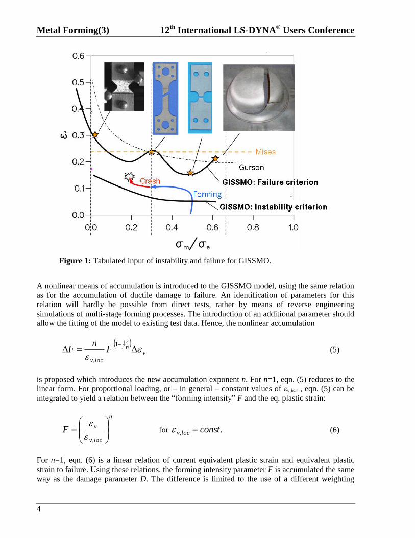
In combination with the treatment of material instability a damage threshold can be defined. As

soon as the damage parameter D reaches this value damage and flow stress will be coupled. The

current implementation allows for to either enter a damage threshold as a fixed input parameter

or to use the damage value corresponding to the instability point. As the post-critical range of

deformation is reached a value of critical damage Dcrit is determined and used for the calculation

of the effective stress tensor:

m

crit

crit

D

DD

11* for critDD (8)

The fading exponent m which can be defined depending on the actual element size governs the

rate of stress fading and thus influences directly the amount of energy that is dissipated during

element fade-out.

Figure 2: Coupling of the damage (left), influence of the fading exponent (right).



6

This strategy allows for regularizing not only fracture strains but also the energy consumed

during the post-critical deformation. A reasonably good regularization of the resulting

engineering stress-strain curves in tensile tests with different mesh sizes can be achieved.

Setup and Analysis of Material Tests

In the first instance information from real material tests has to be gathered. The triaxiality-

dependent failure strain which makes up a principal part of the GISSMO model leads to the need

for conducting experiments with different shaped specimen. In general, all load cases relevant to

the considered material card have to be assessed experimentally. In Figure 3 a choice of used

specimen shapes is shown.

For the evaluation of the measured data all specimen have to be simulated. By using

measurement of force and local displacement as in the test, a direct comparison of experiment

and simulation can be achieved.

One of the most important observations coming from the simulation is that the critical elements

of the computed specimen almost never follow a path of constant triaxiality during loading. Due

to geometrical changes of the section over deformation, a path of varying triaxiality is followed.

This effect is even more pronounced the more ductile a material is. As can be seen in Figure 4

the triaxiality measured in a critical element changes during loading for most specimen types.

This effect has to be taken into account while creating a material card, which basically means the

determination of failure strain will not be a straightforward process.

Figure 3: Different specimen shapes and possible element sizes for discretization.

12th


7

In this study, the following geometries were selected to create a GISSMO material card:

- Uniaxial tensile test with a parallel section

- Notched tensile test with a small notch radius

- Shear test

The experimental setups of these three tests appear quite similar, which allows for the use of a

standard tensile testing machine for all of them. Clamped at both ends each specimen undergoes

a displacement controlled loading at which the external tension or shear force is detected by load

cells. Sensors note the translation of two points to get the displacement relative to each other.

Alternatively, the elongation can be figured out by means of optical measuring techniques like

ARAMIS, for example. The resulting force vs. local displacement curves can easily be converted

into engineering stress vs. engineering strain curves considering the initial cross-section area of

the specimen and the initial gauge length between the two observed points. After filtering and

smoothing the raw data the curves serve as basis for further analyses.

The described practical procedure is reproduced within a finite element simulation. In order to

represent the real physical behavior of the material the LS-DYNA®

models are finely discretized

using shell elements with a characteristic element length of approximately 0.5mm. The boundary

conditions and the evaluation of the displacement and applied force correspond to the

experimental setup.

Calibration of a GISSMO Material Card

Yield curve

In this case the plasticity is captured by the elastic-plastic constitutive model *MAT_024

considering isotropic hardening. Based on the von Mises flow rule the implied yield curve has to

Figure 4: Equivalent plastic strain vs. triaxiality in critical elements.



8

be figured out from experimental results. Searching for effective stress vs. effective plastic strain

the quasistatic tensile test curve can be used as reference. Since the specimen deforms uniformly

before necking the engineering stress-strain curve in this part is directly converted into the

effective true (or logarithmic) values:

E

truetrueplasttrueengtrue

engengtrue

,,1ln

1

(9)

Beyond the point of uniform expansion the yield curve is fitted iteratively by reverse

engineering. Individual or analytical approaches allow to determine the post-critical behavior

until failure. The optimization tool LS-OPT® offers an efficient way for finding a suitable yield

curve as discussed by Witowski et al. (2011). When using the so extracted stress-strain values, a

comparison of the result of a simulated tensile test show excellent correlation with the measured

test curve. As no possibility of regularizing the material model is given in *MAT_024 the curve

fitting process is limited to the present mesh size.

Damage and failure

As explained above the plasticity is separately described within the material model

*MAT_PIECEWISE_LINEAR_PLASTICITY. The GISSMO damage model, chosen to describe

damage and failure behavior, is implemented in card 3 and card 4 of the LS-DYNA keyword

*MAT_ADD_EROSION and activated by the first flag IDAM=1 (see Figure 5).

With DMGTYP=1 the damage is accumulated and element failure occurs for D=1. The coupling

of the internally calculated damage to the flow stress depends on several parameters, which are

identified by conducting an optimization procedure. Setting the damage exponent DMGEXP to a

fixed value, the fading exponent FADEXP is obtained by LS-OPT as well as the two load curves

for LCSDG and for ECRIT. The first one defines the equivalent plastic strain to failure vs.

triaxiality, the second one defines the critical equivalent plastic strain vs. triaxiality.

*MAT_PIECEWISE_LINEAR_PLASTICITY

$ MID RO E PR SIGY ETAN FAIL TDEL

10

$ C P LCSS LCSR VP

...

*MAT_ADD_EROSION

$ MID EXCL MXPRES MNEPS EFFEPS VOLEPS NUMFIP NCS

10

$ MNPRES SIGP1 SIGVM MXEPS EPSSH SIGTH IMPULSE FAILTM

$ IDAM DMGTYP LCSDG ECRIT DMGEXP DCRIT FADEXP LCREGD

1 1 100 -200 2 -300 400

$ SIZFLG REFSZ NAHSV LCSRS SHRF BIAXF

Figure 5: LS-DYNA input for GISSMO.

12th


9

Within the optimization loop, all three above mentioned coupon tests are computed and

evaluated. The progression of each engineering stress-strain curve is compared to the

experimental results aiming at a perfect correlation between both curves. Likewise the difference

in the engineering failure strains is minimized. Five points with fixed triaxiality build the load

curve for LCSDG where the corresponding values for equivalent plastic strain to failure are to be

found by LS-OPT. The critical equivalent plastic strain represents the first occurrence of

instability and therefore the start of coupling the damage to the flow stress. As necking in shear

loading cases is unknown, the value in the ECRIT curve is set to an arbitrary high value, whereas

the beginning of coupling for plane strain is optimized. The point of uniform expansion taken

from tensile test curves delivers the critical strain for the triaxiality of uniaxial tension (i.e. 1/3).

After a few iterations a fading exponent FADEXP and load curves for LCSDG and ECRIT are

obtained showing very good correlations between the test and simulation data in all three

calculated load cases.

Regularization

The identified parameters are initially fitted to only one – rather small – element size (0.5mm).

Due to reasons of cost-effectiveness, full-scale car crash simulations have to be done using mesh

sizes far more coarse. Therefore, the need for regularizing the material card arises. For this

reason a uniaxial tensile test specimen large enough for being discretized with mesh sizes >3mm

has to be used for this purpose. Having a long parallel section (gauge length approximately

80mm), this specimen is simulated with all different mesh sizes considered.

If no experimental data are available for this geometry the engineering stress-strain curve

resulting from a 0.5mm mesh computation serves as reference for the validation of larger

element sizes. This method is called the “virtual tensile test”. The GISSMO damage model offers

the possibility to regularize the fading exponent and the equivalent plastic strain to failure. With

a tabulated input of FADEXP the exponent is defined in dependency of the characteristic

element length. The load curve for LCREGD gives mesh-dependent factors for the failure strain

load curve LCSDG with decreasing values for larger element sizes.

0.5mm 1mm 2.5mm 5mm 10mm

Figure 6: Differently discretized models of a tensile test specimen.



10

As can be seen in Figure 7, a reasonably good regularization can be achieved using these

parameters. In LS-DYNA version 971 R5 or later, two additional features were added that allow

to set limits for the scaling factors at triaxiality=0 (shear, the new parameter is called SHRF) or

at triaxiality=2/3 (biaxial, here the new parameter is called BIAXF). This approach is intended to

further improve regularization capabilities for stress states other than uniaxial tension.

Conclusions

In the present work an effective preparation of a material card for the GISSMO damage model

has been described suitable for capturing the physics of ductile damage and failure in a variety of

stress states and for different materials. Some methods of numerical optimization have been

introduced showing a user-friendly and simple input of material parameters. In order to improve

the accuracy of specific values depending on the triaxiality more experimental tests with

differently shaped specimen will have to be conducted and evaluated.

Further research work will be done concerning the calibration of the underlying plasticity model.

As the yield curve is currently fitted to the uniaxial tension test the engineering stress-strain

curve resulting from simulating a notched tensile test might be too soft compared to the

experimental data. When damage is coupled to the flow stress and failure occurs it might not

help to compensate the difference.

Another field of interest will be the correct specification of instability applying analytical

approaches. Particularly with regard to higher triaxialities the identification of above mentioned

reduction parameters SHRF and BIAXF will have to be investigated.

References

Bai, Y.; Wierzbicki, T.: Forming Severity Concept for Predicting Sheet Necking Under Complex Loading Histories.

Int. Journal of Mechanical Sciences 50, p. 1012-1022, 2008.

Barlat, F.; Lian, J.: Plastic behaviour and stretchability of sheet metals. Part I: A yield function for orthotropic sheets

under plane stress conditions. Int. Journal of Plasticity 5, pp. 51-66, 1989.

De Borst, R.; Sluys, L. J.; Mühlhaus, H.-B.; Pamin, J.: Fundamental Issues in Finite Element Analyses of

Localization of Deformation. Engineering Computations 10, p. 99-121, 1993.

Figure 7: Uniaxial tensile test, regularized stress-strain curves for different element sizes.

12th


11

Haufe, A.; Neukamm, F.; Feucht, M.; Borvall, Th.: A Comparison of recent Damage and Failure Models for Steel

Materials in Crashworthiness Application in LS-DYNA, 11th International LS-DYNA Users Conference 2010,

Dearborn, MI, USA, June 6-8, 2010.

Johnson, G. R.; Cook, W. H.: Fracture Characteristics of Three Metals Subjected to Various Strains, Strain Rates,

Temperatures and Pressures. Eng. Fracture Mechanics 21, p. 31-48, 1985.

Lemaitre, J.: A Continuous Damage Mechanics Model for Ductile Fracture. Journal of Engineering Materials and

Technology 107, p. 83-89, 1985.

Neukamm, F.; Feucht, M.; Haufe, A.: Considering damage history in crashworthiness simulations, 7th European LS-

DYNA Conference, Salzburg, Austria, May 14-15, 2009.

Weck, A.; Wilkinson, D. S.; Toda, H.; Maire, E.: 2D and 3D Visualization of Ductile Fracture. Advanced

Engineering Materials 8 (6), p. 469-472, 2006.

Witowski, K.; Feucht, M.; Stander, N.: An Effective Curve Matching Metric for Parameter Identification using

Partial Mapping, 8th European LS-DYNA Users Conference, Strasbourg, France, 2011.



12

Documents

On parameter identification for the GISSMO damage model