ON OPTIMAL OPERATING POLICIES OF EPQ MODEL WITH TIME ... fileinventory model for deteriorating items over a ﬁnite planning horizon and a linear time-varying demand with a ﬁnite

International Journal of Advances in Mathematics

Volume 2019, Number 5, Pages 35-56, 2019

eISSN 2456-6098

c© adv-math.com

ON OPTIMAL OPERATING POLICIES OF EPQ MODEL WITH

TIME-DEPENDENT REPLENISHMENT AND DETERIORATION HAVING

SELLING PRICE DEPENDENT DEMAND

K.SRINIVAS RAO1 and S.ACHYUTA∗

1DEPARTMENT of STATISTICS, ANDHRA UNIVERSITY,

VISAKHAPATNAM-530 003, India.∗A.U.PLOT: 77/X1, M.V.P.COLONY,

VISAKHAPATNAM -530 017, India.

E-mail: [email protected]

ABSTRACT. EPQ Models are more important for scheduling the production processes and manufacturing units. In this paper,

we study an Economic Production Quantity Model with the assumption that the replenishment is time-dependent. It is fur-

ther assumed that the rate of deterioration is also linearly dependent on time. Using differential equations the instantaneous

state of inventory is derived. With suitable cost considerations, the total cost function and profit rate function is obtained. By

maximizing the profit rate function the optimal policies are derived. Through numerical illustrations, the solution procedure of

the model is demonstrated. The sensitivity analysis of the model reveals that the replenishment parameters and deterioration

parameters have a significant influence on the operating policies.

1 Introduction

Economic Production Quantity models play a dominant role in the analysis of Production process, Warehouse

Management, Market yards etc., in various practical situations the economic production quantity is dependent

* Corresponding Author.

Received March 11, 2019; revised May 17, 2019; Accepted June 01, 2019.

2010 Mathematics Subject Classification: 90B05.

Key words and phrases: EPQ Model, Time-Dependent Deterioration, Selling Price Deterioration, Time- Dependent Replenish-

ment.

This is an open access article under the CC BY license http://creativecommons.org/licenses/by/3.0/.

35

K.SRINIVAS RAO and S.ACHYUTA 36

on, through the constituent process of the model viz., 1.) Replenishment 2.) Demand 3.) Nature of the commodity.

Much work has been reported regarding EPQ models with finite and infinite rates of replenishment. But in

many practical situations the replenishment may or may not be finite but varying depending on time. Due to

variations,in the procurement, transportation, storage capacity etc. Little work has been reported in the literature

regarding EPQ models with time-dependent replenishment.

Mak (1982) developed a production lot size model which deals with an unfilled order backlog for an inven-

tory model with exponential decaying items. Chowdhary and Chaudhuri (1983) obtained an inventory model for

deteriorating items with a finite rate of production and the constant rate of deterioration for both deterministic

and probabilistic cases. Su, et al. (1999) developed a deterministic production inventory model for deteriorat-

ing items with an exponential declining demand over a fixed time and production dependent demand. Mandal

and Phaujdar (1989) obtained a single item stock control model with shortages for deteriorating items having

a uniform rate of production and variable demand is dependent on instantaneous inventory level. Sujit and

Goswami (2001) considered a replenishment policy for items with finite production rate and fuzzy deterioration

rate. Here, the deterioration rate is considered to solve the Economic Production Quantity (EPQ) model. The

production quantity due to the faulty/aged machine is also studied. Sana, et al. (2004) presented a production

inventory model for deteriorating items over a finite planning horizon and a linear time-varying demand with a

finite production rate, shortages. Balkhi (2001) considered a generalized production lot size inventory model for

deteriorating items over finite planning where the demand, production, and deteriorating rates were assumed to

be known and continuous function of time. Samanta and Roy (2004) developed a continuous production control

inventory model for items deteriorating exponentially with time and where the two different rates of production

are available and it is possible that production started at one rate and after some time it may be switched over

to another rate. Lin and Gong (2006) studied a production inventory system of deteriorating items subjected to

random machine breakdowns with fixed repair time allowing price discount using the permissible delay in pay-

ments. Chen (2008) discussed economic production run length and warranty period for products with Weibull

lifetime. Miirzazadeh, et al. (2009) discussed an inventory model under uncertain inflationary conditions, finite

production rate and inflation dependent demand rate for deteriorating items with shortages. Lee and Hsu (2009)

developed a two-warehouse inventory model for deteriorating items with time-dependent demand. The vari-

ation in production cycle times to determine the number of production cycles and the times for replenishment

during a finite planning horizon is considered. Manna and Chiang (2010) developed two deterministic economic

production quantity (EPQ) models with and without shortages of Weibull distribution, deteriorating items with

demand rate as a ramp type function of time. Sridevi, et al. (2010) developed and analyzed an inventory model

with the assumption that the rate of production is random and follows a Weibull distribution and the demand

is a function of the selling price. By maximizing the profit rate function they obtained the optimal ordering and

pricing policies of the model. The sensitivity of the model with respect to the parameters and costs was also

analyzed. Tripathy, et al (2010) developed an EPQ model with no shortages for items with trine varying holding

cost, linear deterioration, and constant production and demand rates. Partially deteriorated items were allowed

to float into the market with a discount. Manna and Chiang (2010) developed two deterministic Economic Pro-

duction Quantity models for Weibull distribution deteriorating items with demand rate as ramp type function


of time. Sarkar and Moon (2011) studied a finite time production inventory model for stochastic demand with

shortages and the effect of inflation. A certain percentage of products were of imperfect quality and the lifetime

of a defective item was assumed to follow a Weibull distribution. They derived profit function by using both

a general distribution of demand and the uniform rectangular distribution of demand. The production rate of

the inventory model is considered to be constant. Srinivasa Rao and Essey Kebede Muluneh (2012) developed a

production inventory model for deteriorating items and analyzed with the assumption that the production rate

is dependent on stock on hand. It is further assumed that the lifetime of the commodity is random and follows

a three-parameter Weibull distribution and demand rate is a function of both selling price and time. Palanivel

& Uthayakumar (2013), developed an Economic Production Quantity (EPQ) model with price and advertisement

dependent demand under the effect of inflation and time value of money. The selling price of a unit is deter-

mined by a mark-up over the production cost. In this model, the holding cost per unit of the item per unit time

is assumed to be an increasing linear function of time spent in storage. Hui-Ming Teng (2013), studied an eco-

nomic production quantity model for deteriorating items in which backorder is allowed. The selling price of

backorder depends on the customers that are willing to purchase the items under the condition that they receive

their orders after a certain fraction of waiting time. Anand and Jagat Veer Singh (2013) developed a production

inventory model for decaying items with multi-variate demand and variable holding cost. Demand rate function

depends upon the present inventory level and the selling price per unit during the production phase. Shortages

are permitted with partial backlogging. The backlogging rate is waiting time for the next replenishment. Sanjay

Sharma and Singh (2013), developed a model with the concept of space restriction in which demand is exponen-

tial, and deterioration is time-dependent. Production is taken as a function of demand. Ashendra Kumar Saxena

and Ravish Kumar Yadav (2013) studied an Economic Production Quantity (EPQ) model for the noninstanta-

neous deteriorating item in which production and demand rates are constant and the holding cost varies with

quadratic in time. Srinivasa Rao, et al. (2013), developed and analyzed an EPQ model for deteriorating items

with stock-dependent production rate and Pareto rate of decay. Meenakshi Srivastava & Ranjana Gupta (2013),

studied continuous production inventory model for deteriorating items with time and price-dependent demand

under markdown policy for both fresh and deteriorated units. Da Wen, Pan Ershun, Wang Ying and Liao Wenzhu

(2014), integrated predictive maintenance into EPQ models in which autoregressive integrated moving average

model is adopted to predict system’s healthy indicator due to machine degradation. Palanivel & Uthayakumar

(2014), developed an Economic Production Quantity (EPQ) model under the effect of inflation and time value of

money. The selling price of a unit is determined by a mark up over the production cost. They have considered

three types of continuous probabilistic deterioration function, and also considered that the holding cost of the item

per unit time is assumed to be an increasing linear function of time spent in storage. Himani Dem, Singh, Jitendra

Kumar (2014), Studied, an Economic Production Quantity model (EPQ) model for finite production rate and de-

teriorating items with time-dependent trapezoidal demand. An EPQ model is formulated for deteriorating items

with time-dependent demand rate and time-dependent production rate. To retain the confidence of the buyers

the machine reliability, flexibility and packaging cost are considered. Shortages are allowed and it is completely

backlogged. A mathematical model has been presented to find the optimal order quantity and total cost. The

holding cost, setup cost, deterioration cost, labour cost for packing, the material cost for packing, shortage cost,


production cost involved in this model are taken as triangular fuzzy numbers. To validate the optimal solution,

a numerical example is provided. To analyze the effect of variations in the optimal solution with respect to the

change in one parameter at a time, sensitivity analysis is carried out. Ankit Bhojak, Gothi (2015), they developed

an inventory model to determine the economic production quantity for deteriorating items under time depen-

dent demand. Inventory holding cost was taken as a linear function depending upon time. A combination of two

parameters and three-parameter Weibull distribution is considered for the deterioration of units over a period of

time. For practical applicability, shortages were allowed to occur. Besides that, they have assumed that demand

is a linear and also quadratic function of time at different time intervals. A numerical example is given for the

developed model with its sensitivity analysis. Kirtan Parmar and Gothi (2015), they have analyzed a production

inventory model for deteriorating items with time-dependent holding cost. Three parameters Weibull distribution

was assumed for time to deterioration of items. Shortages were allowed to occur. The derived model was illus-

trated by a numerical example and its sensitivity analysis is carried out. Kousar Jaha Begum and Devendra (2016)

developed and analyzed an E.P.Q model with the assumptions that the lifetime of a commodity is random and

follows a Generalized Pareto Distribution. Dhir Singh & Singh (2017), developed economic production quantity

(EPQ) model for deteriorating product with time dependent demand and the time dependent inventory carrying

cost. There, it was assumed that the production rate at any instant depends on both the stock and the demand for

the product. To make the model more realistic, the shortages were allowed and partially backlogged. The back

ordering rate was taken as a decreasing function of waiting time for the next refill. Khedlekar, Namedeo, Nigwal

(2018), in the paper, made an attempt to develop an economic production quantity model using optimization

method for deteriorating items with production disruption. The disruption in a production system occurs due to

labour problem, machines breakdown, strikes, political issue, and weather disturbance, etc. This leads to delay in

the supply of the products, resulting customer to approach other dealers for the products. The optimal production

and inventory plan were provided. So that the manufacturer can reduce the loss occurred due to disruption. Nita

Shah and Chetansinh Vaghela (2018), developed this paper to establish an economic production quantity (EPQ)

model for deteriorating items with both up-stream and down-stream trade credits. Here, In practice, trade credit

induces more sales over time by allowing customers to purchase without immediate cash. Nita Shah, Mrudul

Jani, Urmila Chaudhari (2018), In this article, a production inventory model with dynamic production rate and

production time dependent selling price has been presented. They considered the product with constant deterio-

ration rate which is a very realistic approach. It is also considered that the production rate is a decreasing function

of the inverse efficiency of the system.

Hence, in this paper, we develop and analyze EPQ models with time dependent replenishment. Here, it is

assumed that the replenishment is linearly dependent and is of the form R (t) = a+ bt, where ‘a’ and ‘b’ are two

parameters. This replenishment also includes a constant rate of replenishment when b = 0. Another important

consideration in EPQ models is demand. In this model, it is assumed that demand is the function of selling

price and is of the form l (s) =(d – f s

)where d and f are parameters and ‘s’ is the selling price. Further, it is

assumed that the lifetime of the commodity is finite and depends on time. This is represented with time dependent

deterioration rate. Here, it is assumed that the instantaneous rate of deterioration is linearly dependent on time

and is of the formh(t) = a + bt. This includes the increasing/decreasing/constant rate of deterioration.


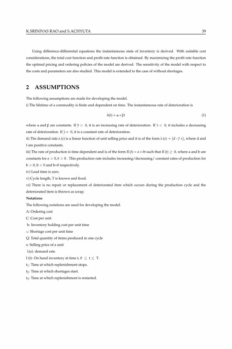
Using difference-differential equations the instantaneous state of inventory is derived. With suitable cost

considerations, the total cost function and profit rate function is obtained. By maximizing the profit rate function

the optimal pricing and ordering policies of the model are derived. The sensitivity of the model with respect to

the costs and parameters are also studied. This model is extended to the case of without shortages.

2 ASSUMPTIONS

The following assumptions are made for developing the model.

i) The lifetime of a commodity is finite and dependent on time. The instantaneous rate of deterioration is

h(t) = a + bt (1)

where a and b are constants. If b > 0, it is an increasing rate of deterioration. If b < 0, it includes a decreasing

rate of deterioration. If b = 0, it is a constant rate of deterioration.

ii) The demand rate l (s) is a linear function of unit selling price and it is of the form l (s) =(d – f s

), where d and

f are positive constants.

iii) The rate of production is time dependent and is of the form R (t) = a + bt such that R (t) ≥ 0, where a and b are

constants for a > 0, b > 0 . This production rate includes increasing/decreasing/ constant rates of production for

b > 0, b < 0 and b=0 respectively.

iv) Lead time is zero.

v) Cycle length, T is known and fixed.

vi) There is no repair or replacement of deteriorated item which occurs during the production cycle and the

deteriorated item is thrown as scrap.

Notations

The following notations are used for developing the model.

A: Ordering cost

C: Cost per unit

h: Inventory holding cost per unit time

p: Shortage cost per unit time

Q: Total quantity of items produced in one cycle

s: Selling price of a unit

l(s): demand rate

I (t): On hand inventory at time t, 0 ≤ t ≤ T.

t1: Time at which replenishment stops.

t2: Time at which shortages start.

t3: Time at which replenishment is restarted.


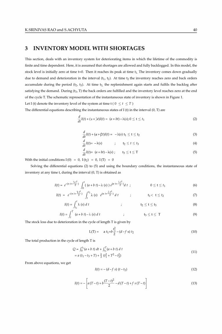
3 INVENTORY MODEL WITH SHORTAGES

This section, deals with an inventory system for deteriorating items in which the lifetime of the commodity is

finite and time dependent. Here, it is assumed that shortages are allowed and fully backlogged. In this model, the

stock level is initially zero at time t=0. Then it reaches its peak at time t1. The inventory comes down gradually

due to demand and deterioration in the interval (t1, t2). At time t2 the inventory reaches zero and back orders

accumulate during the period (t2, t3). At time t3, the replenishment again starts and fulfils the backlog after

satisfying the demand. During (t3, T) the back orders are fulfilled and the inventory level reaches zero at the end

of the cycle T. The schematic representation of the instantaneous state of inventory is shown in Figure 1.

Let I (t) denote the inventory level of the system at time t ( 0 ≤ t ≤ T )

The differential equations describing the instantaneous states of I (t) in the interval (0, T) are

ddt

I(t) + (a + bt)I(t) = (a + bt) – l(s); 0 ≤ t ≤ t1 (2)

ddt

I(t) + (a + bt)I(t) = – l(s) t1 ≤ t ≤ t2 (3)

ddt

I(t)= – l(s) ; t2 ≤ t ≤ t3 (4)

ddt

I(t)= (a + bt) – l(s) ; t3 ≤ t ≤ T (5)

With the initial conditions I (0) = 0, I (t2) = 0, I (T) = 0

Solving the differential equations (2) to (5) and using the boundary conditions, the instantaneous state of

inventory at any time t, during the interval (0, T) is obtained as

I(t) = e–(a t+ b t2

2 )∫ t

0( (a + b t) – l (s) ) e(a t+ b t2

2 )d t ; 0 ≤ t ≤ t1 (6)

I(t) = e–(a t+ b t2

2 )∫ t2

tl (s) e(a t+ b t2

2 ) d t ; t1< t ≤ t2 (7)

I(t) =∫ t

t2

l (s) d t ; t2 ≤ t ≤ t3 (8)

I(t) =∫ T

t(a + b t) – l (s) d t ; t3 ≤ t ≤ T (9)

The stock loss due to deterioration in the cycle of length T is given by

L(T) = a t1+bt212

– (d – f s) t2 (10)

The total production in the cycle of length T is

Q =∫ t1

0 (a + b t) dt +∫ T

t3(a + b t) d t

= a (t1 – t3 + T) + b2 (t2

1 + T2 – t23)

(11)

From above equations, we get

I(t) = – (d – f s) (t – t2) (12)

I(t) = –

[a (T – t) + b

(T – t)2

2– d (T – t) + f s (T – t)

](13)


When t = t3, the above equations become

I (t3) = – (d – f s) (t3 – t2) (14)

I (t3) = –

[a (T – t3) + b

(T – t3)2

2– d (T – t3) + f s (T – t3)

](15)

On equating the equations (14) and (15), and by simplifying them and expressing t2 in terms of t3 as,

t2 = t3 –1

d – f s

[a (T – t3) +

b2

(T2 – t2

3

)+(d – f s

)(T – t3)

]= y say (16)

Let K (t1,t2, t3, s) be the total cost per unit. The total cost is the sum of the setup the cost per unit time,

purchasing cost per unit time, holding cost per unit time and shortage cost per unit time. Then K (t1, t3, s)

becomesK(t1, t2, t3, s) = A

T + CQT + h

T

[∫ t10 I(t) dt +

∫ t2t1

I(t) dt]

+ pT

[–∫ t3

t2I(t) dt –

∫ Tt3

I(t) dt]

Substituting the values of I (t) and Q, given in the above equations in Equation

K(t1, t3, s) = AT + C

T

{(a (t1 – t3 + T) + b

2 (t21 + T2 – t2

3))}

+ hT

{∫ t10 e–(a t+b t2

2 )(∫ t

0((a + b u) – (d – f s)

)e(a u+b u2

2 ) d u)

d t

+∫ y(t)

t1e–(a t+b t2

2 )(∫ y(t)

t (d – f s) e(a u+b u2

2 ) d u)

d t]

+ pT

{ ∫ t3y(t)

(∫ ty(t)( d – f s) d u

)d t +

∫ Tt3

(∫ Tt((a + b u) – (d – f s)

)d u)

d t}

On integrating and simplifying the above equation we get

K(t1, t3, s) = AT + C

T

{a(t1 – t3 + T) + b

2 (t21 + T2 – t2

3)}

+ hT

{(a –(d – fs

)) [∫ t10 e–(at+b t2

2 )(∫ t

0 e(au+b u2

2 ) du)

dt]

+ b[∫ t1

0 e–(at+b t2

2 )(∫ t

0 u e(au+b u2

2 )du)

dt]

+ (d – fs)∫ y(t)

t1e–(at+b t2

2 )(∫ y(t)

t e(au+b u2

2 )du)

dt}

+ pT

{ (a – (d – fs)

) ( T2

2 – Tt3 + t232

)+ b

(T3

3 – T2t32 + t3

36

) }

Let P (t1, t3, s) be the profit rate function. Since the profit rate function is the total revenue per unit time minus

total cost per unit time, we have

P (t1, t3, s) = s l (s) – K ( t1, t3, s ) (17)


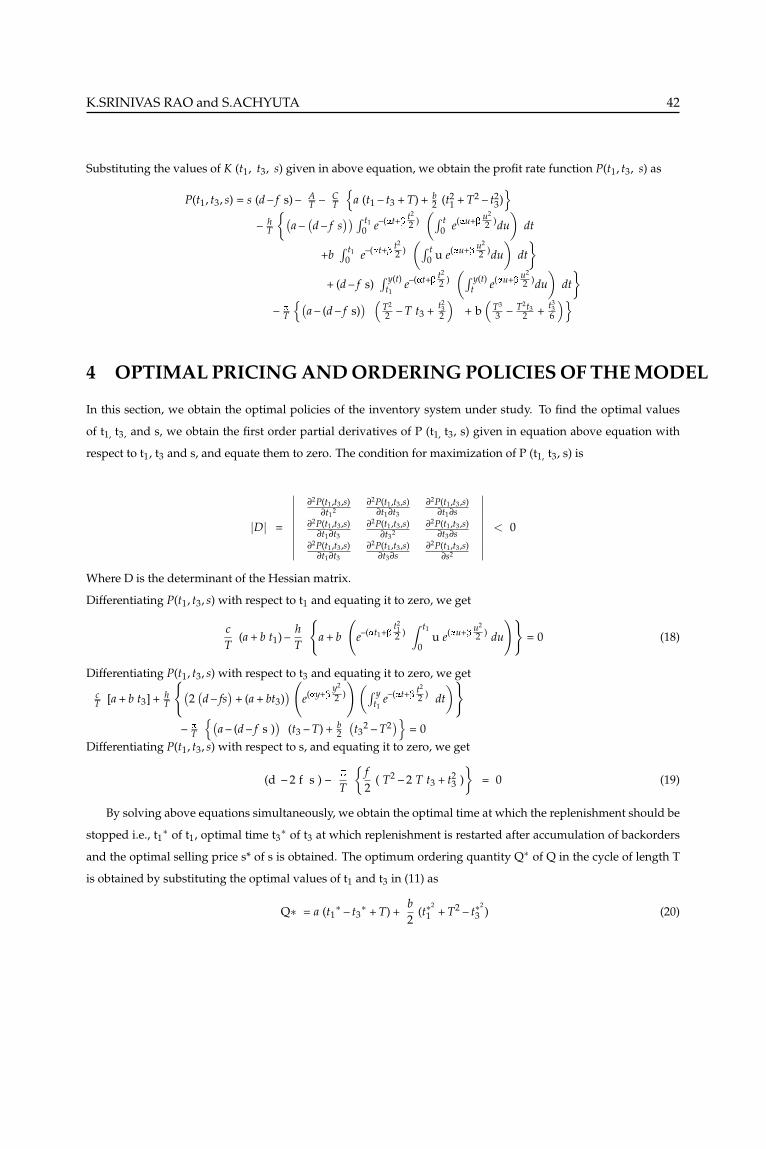
Substituting the values of K (t1, t3, s) given in above equation, we obtain the profit rate function P(t1, t3, s) as

P(t1, t3, s) = s (d – f s) – AT – C

T

{a (t1 – t3 + T) + b

2 (t21 + T2 – t2

3)}

– hT

{(a –(d – f s

)) ∫ t10 e–(at+b t2

2 )(∫ t

0 e(au+b u2

2 )du)

dt

+b∫ t1

0 e–(at+b t2

2 )(∫ t

0 u e(au+b u2

2 )du)

dt}

+ (d – f s)∫ y(t)

t1e–(at+b t2

2 )(∫ y(t)

t e(au+b u2

2 )du)

dt}

– pT

{(a – (d – f s)

) ( T2

2 – T t3 + t232

)+ b

(T3

3 – T2t32 + t3

36

)}

4 OPTIMAL PRICING AND ORDERING POLICIES OF THE MODEL

In this section, we obtain the optimal policies of the inventory system under study. To find the optimal values

of t1, t3, and s, we obtain the first order partial derivatives of P (t1, t3, s) given in equation above equation with

respect to t1, t3 and s, and equate them to zero. The condition for maximization of P (t1, t3, s) is

|D| =

∣∣∣∣∣∣∣∣∣∂2P(t1,t3,s)

∂t12

∂2P(t1,t3,s)∂t1∂t3

∂2P(t1,t3,s)∂t1∂s

∂2P(t1,t3,s)∂t1∂t3

∂2P(t1,t3,s)∂t3

2∂2P(t1,t3,s)

∂t3∂s∂2P(t1,t3,s)

∂t1∂t3

∂2P(t1,t3,s)∂t3∂s

∂2P(t1,t3,s)∂s2

∣∣∣∣∣∣∣∣∣ < 0

Where D is the determinant of the Hessian matrix.

Differentiating P(t1, t3, s) with respect to t1 and equating it to zero, we get

cT

(a + b t1) –hT

{a + b

(e–(at1+b

t212 )∫ t1

0u e(au+b u2

2 ) du

)}= 0 (18)

Differentiating P(t1, t3, s) with respect to t3 and equating it to zero, we get

cT [a + b t3] + h

T

{(2(d – fs

)+ (a + bt3)

) (e(ay+b

y2

2 )

)(∫ yt1

e–(at+b t2

2 ) dt)}

– pT

{(a – (d – f s )

)(t3 – T) + b

2(t3

2 – T2)} = 0Differentiating P(t1, t3, s) with respect to s, and equating it to zero, we get

(d – 2 f s ) –p

T

{f2

( T2 – 2 T t3 + t23 )}

= 0 (19)

By solving above equations simultaneously, we obtain the optimal time at which the replenishment should be

stopped i.e., t1∗ of t1, optimal time t3

∗ of t3 at which replenishment is restarted after accumulation of backorders

and the optimal selling price s* of s is obtained. The optimum ordering quantity Q∗ of Q in the cycle of length T

is obtained by substituting the optimal values of t1 and t3 in (11) as

Q∗ = a (t1∗ – t3

∗ + T) +b2

(t∗2

1 + T2 – t∗2

3 ) (20)


5 NUMERICAL ILLUSTRATIONS

Here, we deal with the solution procedure of the model through a numerical illustration by obtaining the replen-

ishment (production) uptime, replenishment (production) downtime, optimal selling price, optimal quantity and

profit of an inventory system. It is assumed that the commodity is of the deteriorating nature and shortages are

allowed and fully backlogged. For demonstrating the solution procedure of the model the deteriorating parame-

ter a is considered to vary between 0.3 to 0.8, the values of the other parameters and costs associated with model

are: a = 3, 4, 5; b = 1, 1.5, 2; b = .1, .2, .3

A = 100, 200, 300; C = 2, 3, 4; d = 500, 600, 700; f = 10, 20, 30; h =0.012, 0.014, 0.02; p = .035, .04, .045; T = 12 months

Substituting these values, the optimal selling price, the optimal ordering quantity Q*, replenishment time,

optimal value of time and total profit are computed and presented in Table 1.

As the demand parameter d is increasing, from 500 to 700, there is a decrease in optimal ordering quantity

Q*, it decreases from 124.113 to 110.481, as the optimal value of t1∗ increases from 1.089 to 3.138, the optimal

replenishment time t3∗ increases from 7.131 to 8.694, the optimal selling price s∗ is increasing from 12.493 to 17.502

and the profit is increasing from 3069.16 to 6069.41. As the demand parameter f, is increasing from 10 to 30, the

optimal ordering quantity Q* is decreasing from 124.126 to 124.100, the optimal value of t1∗ increases from 1.088 to

1.091, the optimal replenishment time t3∗ increases from 7.130 to 7.133, the optimal selling price s∗ decreases from

24.993 to 8.326 and profit rate decreases from 6194.16 to 2027.50. As the ordering cost A increases, from 100 to 300,

all the values remain constant, except for the profit. It decreases from 3077.50 to 3060.83. When the cost per unit

C increases, from 2 to 4, there is an increase in optimal ordering quantity Q*, it increases from 107.363 to 124.113,

the optimal value of t1∗ decreases from 4.986 to 1.089, the optimal replenishment time t3

∗ decreases from 9.856

to 7.131, the optimal selling price s∗ is decreasing from 12.504 to 12.493 and the profit decreases from 3088.16 to

3069.16. As the Production parameters ‘a’ increases, from 3 to 5, there is an increase in optimal ordering quantity

Q*, from 112.986 to 124.113, the optimal value of t1∗ decreases from 2.068 to 1.089, the optimal replenishment

time t3∗ decreases from 7.430 to 7.131, the optimal selling price s∗ increases from 12.491 to 12.493 and the profit

decreases from 3073.45 to 3069.16. When ‘b’ is increasing, from 1 to 2, there is an increase in optimal ordering

quantity Q*, the increase is from 63.379 to 124.113, the optimal value of t1∗ decreases from 3.830 to 1.089, the

optimal replenishment time t3∗ decreases from 9.670 to 7.131, the optimal selling price s∗ is decreasing from

12.508 to 12.493 and the profit decreases from 3082.71 to 3069.16.

When the deteriorating parameter a increases, from 0.3 to 0.8, we observe that there is an increase in optimal

ordering quantity Q*, from 124.113 to 126.168, the optimal value of t1∗ increases from 1.089 to 1.677, the optimal

replenishment time t3∗ increases from 7.131 to 7.261 and the optimal selling price s∗ is increasing from 12.493 to

12.495 and the profit decreases from 3069.16 to 3068.02. When b is increasing from 0.1 to 0.3, there is a decrease in

optimal ordering quantity Q*, from 126.847 to 122.549, the optimal value of t1∗ increases from 0.781 to 1.335, the

optimal replenishment time t3∗ increases from 6.876 to 7.306, the optimal selling price s∗ is increasing from 12.489

to 12.496 and the profit is decreasing from 3069.96 to 3068.52. As the shortage cost per unit time p increases, from

0.035 to 0.045, there is a decrease in optimal ordering quantity Q*, from 131.283 to 117.963, the optimal value of t1∗

increases from 0.422 to 1.673, the optimal replenishment time t3∗ increases from 6.514 to 7.671, the optimal selling


price s∗ increases from 12.489 to 12.497 and the profit increases from 3068.47 to 3069.57.

Inventory holding cost per unit time h increases, from 0.012 to 0.02, there is an increase in the optimal ordering

quantity Q*, from 124.113 to 129.452, the optimal value of t1∗ increases from 1.089 to 1.716, the optimal replenish-

ment time t3∗ decreases from 7.131 to 7.108, the optimal selling price s∗ increases from 124.113 to 129.452 and the

profit is decreasing from 3069.16 to 3068.23.

6 SENSITIVITY ANALYSIS OF THE MODEL

Sensitivity analysis is carried to explore the effect of changes in model parameters and costs on the optimal poli-

cies, by varying each parameter (-15%,-10%, -5%, 0%, 5%, 10%, 15%) at a time for the model under study. The

results are presented in Table 2.

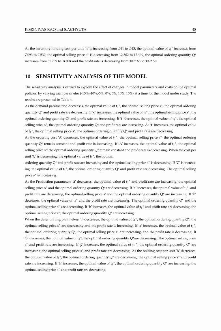
As the demand parameter d decreases, the optimal value of t1∗, the optimal replenishment time t3

∗, the optimal

selling price s∗ and profit rate are decreasing, the optimal ordering quantity Q* is increasing. If, ‘d’ increases,

the optimal value of t1∗, the optimal replenishment time t3

∗, the optimal selling price s∗ and profit rate are in-

creasing, the optimal ordering quantity Q* is decreasing. As ‘f’ decreases, the optimal value of t1∗, the optimal

replenishment time t3∗ decreases and the optimal selling price s∗, the optimal ordering quantity Q* and profit

rate are increasing. If, ‘f’ increases, the optimal value of t1∗, the optimal replenishment time t3

∗ increases and the

optimal selling price s∗, the optimal ordering quantity Q* and profit rate is decreasing. When the ordering cost

‘A’ decreases or increases, the optimal value of t1∗, the optimal replenishment time t3

∗, the optimal selling price

the optimal ordering quantity Q* and profit rate remain constant.

As the cost per unit ‘C’ is decreasing, the optimal value of t1∗, the optimal replenishment time t3

∗, the optimal

selling price s∗ and profit rate are increasing and the optimal ordering quantity Q* is decreasing. When ‘C’ is

increasing, the optimal value of t1∗, the optimal replenishment time t3

∗, the optimal selling price s∗ and profit rate

are decreasing, the optimal ordering quantity Q* is increasing.

If the Production parameters ‘a’ decreases, the optimal value of t1∗, the optimal replenishment time t3

∗, the opti-

mal selling price s∗ and profit rate are increasing, the optimal ordering quantity Q* is decreasing. If ‘a’ increases,

the optimal value of t1∗, the optimal replenishment time t3

∗, the optimal selling price s∗ and profit rate are de-

creasing. The optimal ordering quantity Q* is increasing. If ‘b’ decreases, the optimal value of t1∗, the optimal

replenishment time t3∗, the optimal selling price s∗ and profit rate are increasing. The optimal ordering quantity

Q* is decreasing. If ‘b’ increases, the optimal value of t1∗, the optimal replenishment time t3

∗, the optimal selling

price s∗ and profit rate are decreasing. The optimal ordering quantity Q* is increasing.

As the deteriorating parameters ‘a’ decreases, the optimal value of t1∗, the optimal replenishment time t3

∗, the

optimal ordering quantity Q* are decreasing, the optimal selling price s∗ and profit rate are increasing. If ‘a’

increases, the optimal value of t1∗, the optimal replenishment time t3

∗, the optimal ordering quantity Q* are

increasing, the optimal selling price s∗ and profit rate are decreasing. If b decreases, the optimal value of t1∗, the

optimal replenishment time t3∗ and the optimal selling price s∗are decreasing. The optimal ordering quantity

Q∗ and profit rate are increasing. If b increases, the optimal value of t1∗, the optimal replenishment time t3

∗, the

optimal selling price s∗are increasing, the optimal ordering quantity Q* and profit rate are decreasing.


When the shortage cost per unit p decreases, the optimal value of t1∗, the optimal replenishment time t3

∗, the

optimal selling price s∗ and profit rate are decreasing, the optimal ordering quantity Q* is increasing. If p in-

creases, the optimal value of t1∗, the optimal replenishment time t3

∗, the optimal selling price s∗ and profit rate

are increasing. The optimal ordering quantity Q∗ is decreasing.

As the holding cost per unit ‘h’ decreases, the optimal value of t1∗, the optimal replenishment time t3

∗, the optimal

ordering quantity Q* are decreasing, the optimal selling price s∗ and profit rate are increasing. If ‘h’ increases, the

optimal value of t1∗, the optimal replenishment time t3

∗and the optimal ordering quantity Q* are increasing, the

optimal selling price s∗ and profit rate are decreasing.

7 INVENTORY MODEL WITHOUT SHORTAGES

In this section, the inventory model for deteriorating items without shortages is developed and analyzed. Here

it is assumed that the shortages are not allowed and the stock level is zero at time t=0. The stock level increases

during the period (0, t1) due to excess replenishment after fulfilling the demand and deterioration. The replenish-

ment stops at time t1 when stock level reaches its peak. The inventory decreases gradually due to demand and

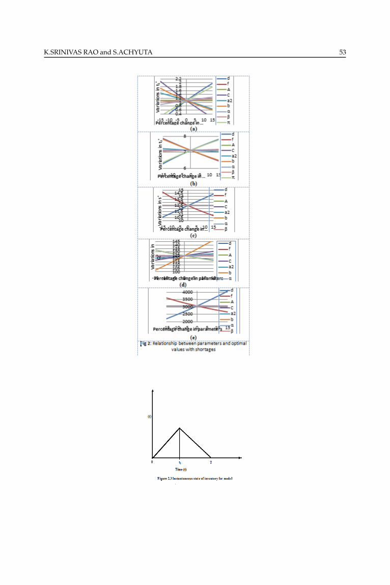
deterioration in the interval (t1, T). At time T the inventory reaches zero. The schematic diagram representing the

instantaneous state of inventory is given in Figure 3.

Let I (t) be the inventory level of the system at a time ‘t’(0 ≤ t ≤ T).

Then the differential equations governing the instantaneous state of I (t) over the cycle of length T areddt I(t) + (a + b t) I(t) = (a + b t) – l (s); 0 ≤ t ≤ t1 (21)

ddt

I( t ) + (a + b t) I( t ) = – l (s) ; t1 ≤ t ≤ T (22)

With the boundary conditions I (T) = 0, I (0) = 0

The instantaneous state of inventory at any given time t during the interval (0, T) is

I(t) = e–(at+bt2/2) [∫ t

0[ (a + bt) – l(s) ] e(at+bt2/2)d t ; 0 ≤ t ≤ t1 (23)

I(t) = e–(a t+b t2/2)∫ T

tl (s) e(a t+b t2/2) d t; t1 ≤ t ≤ T (24)

The production quantity during the cycle time (0, T) is given by

Q = at1 +bt2

12

(25)

Using equations (23) and (24), we obtain the stock loss due to deterioration in this interval (0, T) as the difference

between the total quantity produced and the demand met during (0, T) and is given by

L (T) = at1 + bt212

– l (s) T (26)

This amount of quantity is lost due to deterioration of commodity and is a waste. To obtain the optimal

operating policies one must reduce the stock loss due to deterioration.


Let K (t1, s) be the total cost per unit time. Since the total cost is the sum of the setup cost, cost of units, the

inventory holding cost. Therefore the total cost is

K(t1, s) =AT

+CQT

+hT

[∫ t1

0I(t)dt +

∫ T

t1

I(t)dt]

(27)

Substituting the value of I (t) and Q given in equations (23), (24) and (25) in the equation (27) we obtain K (t1, s) as

K(t1, s) = AT + C

T

(a t1 + b t1

2

2

)+ h

T

{∫ t10 e–(a t+b t2

2 )(∫ t

0((a + bu) –

(d – f s

))e(a u+b u2

2 ) d u)

d t

+∫ T

t1e–(a t+b t2

2 )(∫ T

t(d – f s

)e(a u+b u2

2 ) d u)

d t} (28)

On integrating and simplifying equation (27) we get

K(t1, s) = AT + C

T

(at1 + b t1

2

2

)+ h

T

{(a – (d – f s)

) ∫ t10 e–(at+b t2

2 )(∫ t

0 e(au+b u2

2 )du)

dt

+ b∫ t1

0 e–(at+b t2

2 )(∫ t

0 u e(au+b u2

2 )d u)

d t

+ (d – f s)∫ T

t1e–(at+b t2

2 )(∫ T

t e(au+b u2

2 )d u)

d t} (29)

Let P(t1, s) be the profit rate function. Since the profit rate function is the total revenue per unit time minus total

cost per unit time, we have

P(t1, s) = s l (s) – K (t1, s) (30)

Substituting the value of K(t1, s)given in equation (28), we obtain the profit rate function of P(t1, s) as

P(t1, s) = s (d – f s) – AT – C

T

(a t1 + b t1

2

2

)– h

T

{(a – (d – f s)

) ∫ t10 e–(at+b t2

2 )(∫ t

0 e(au+b u2

2 )d u)

d t

+ b∫ t1

0 e–(at+b t2

2 )(∫ t

0 u e(au+b u2

2 )d u)

d t

+ (d – f s)∫ T

t1e–(at+b t2

2 )(∫ T

t e(au+b u2

2 )d u)

d t} (31)

8 OPTIMAL PRICING AND ORDERING POLICIES OF THE MODEL

This section, we obtain the optimal policies of the inventory system under study. To find the optimal values of

production time t1 and the optimal unit selling price s. We equate the first order partial derivatives of P (t1, s)

with respect to t1 and s, equate them to zero. The condition for maximization of P (t1, s) is

|D| =

∣∣∣∣∣∣∂2P(t1,s)

∂t12

∂2P(t1,s)∂t1∂s

∂2P(t1,s)∂s∂t1

∂2P(t1,s)∂s2

∣∣∣∣∣∣ < 0 where D is the determinant of the Hessian matrix.

Differentiate P (t1, s) with respect to t1 and equating it to zero, we get

CT [a + bt1] – h

T

{(a –(d – f s

) ) [e–(at1+b t1

2

2 ) ∫ t10 e(au+b u2

2 )du]

+ b[

e–(at1+b t12

2 ) ∫ t10 u e(au+b u2

2 ) du]

–(d – f s

) [e–(at1+b t1

2

2 ) ∫ Tt1

e(au+b u2

2 ) du]}

= 0

(??) (??)


Differentiate P (t1, s) with respect to s, and equating it to zero, we get

– hT

{f[∫ t1

0 e–(at+b t2

2 ) ∫ t0 e(au+b u2

2 )du]

dt + f[∫ T

t1e–(at+b t2

2 ) ∫ Tt e(au+b u2

2 )d u]

dt}

= 0(32)

Solving the equations (??) and (32) simultaneously, we obtain the optimal time at which the replenishment is to

be stopped t1∗ of t1 and the optimal unit selling price s∗ of s. The optimum ordering quantity Q∗ of Q in the cycle

of length T is obtained by substituting the optimal values of t1 in (25) as

Q ∗ = at1∗ +

bt21∗

2(33)

9 NUMERICAL ILLUSTRATIONS

In this section, we discuss a numerical illustration of the model. For demonstrating the solution procedure of

the model, the deteriorating parameter ‘a’ is considered to vary .1 to .3, the values of other parameters and costs

associated with the model are:

A = 100, 200, 300; a = 5, 6, 7; b = 1, 2, b =.01, .02, .03, C = 2, 3, 4; d = 400, 500, 600; f = 10, 20, 30; h = 0.011, 0.012,

0.013; T = 12 months

From the table 3, it is observed that the optimal values of t1∗, s∗, Q∗ are obtained for different values of parameters

and costs are shown in table 3.

As the demand parameter d’ is increasing from 400 to 600, there is an increase in optimal ordering quantity Q*,

it increases from 78.887 to 100.006, the optimal value of t1∗ increases from 6.727 to 7.808, the optimal selling price

s∗is increasing from 10.005 to 14.998 and the profit is increasing from 1967.900 to 4467.64. If ‘f’ is increasing from

10 to 30, the optimal value of t1∗ decreases from 7.322 to 7.320, the optimal selling price s∗ is decreasing from

25.001 to 8.334, the optimal ordering quantity Q* decreases from 90.222 to 90.218, the profit rate is decreasing

from 6217.59 to 2050.92.

As the ordering cost ‘A’ increases from 100 to 300, all the values remain constant, except the profit rate which

decreases from 3100.92 to 3084.25. As the cost per unit C increases from 2 to 4, there is decrease in optimal

ordering quantity Q*, it decreases from 90.220 to 57.743, the optimal value of t1∗ decreases from 7.321 to 5.499,

the optimal selling price s∗ is increasing from 12.501 to 12.516 and the profit decreases from 3092.59 to 3080.66.

As the Production parameter ‘a’ increases from 5 to 7, the optimal value of t1∗ decreases from 7.321 to 7.055, the

optimal selling price s∗ increases from 12.501 to 12.503, the optimal ordering quantity Q* increases from 90.222

to 99.163, the profit rate is decreasing from to 3092.59 to 3090.16. As ‘b’ is increasing from 1 to 3. The optimal

value of t1∗ decreases from 8.626 to 6.502, the optimal selling price s∗ increases from 12.493 to 12.507, the optimal

ordering quantity Q* increases from 80.337 to 95.926, the profit rate is decreasing from 3097.83 to 3088.59. As the

deteriorating parameters ‘a’ increases, the optimal value of t1∗ increases from 6.929 to 7.715, the optimal selling

price s∗ is increasing from 12.500 to 12.502, the optimal ordering quantity Q* decreases from 82.667 to 98.097, the

profit rate is decreasing from 3094.28 to 3091.07. If the deteriorating parameters ‘b’ increases, the optimal value

of t1∗ increases from 7.321 to 8.083, the optimal selling price s∗ is decreasing from 12.501 to 12.499, the optimal

ordering quantity Q* increases from 90.220 to 105.759, the profit rate is decreasing from 3092.59 to 3090.45.


As the inventory holding cost per unit ‘h’ is increasing from .011 to .013, the optimal value of t1∗ increases from

7.093 to 7.532, the optimal selling price s∗ is decreasing from 12.502 to 12.499, the optimal ordering quantity Q*

increases from 85.799 to 94.394 and the profit rate is decreasing from 3092.68 to 3092.56.

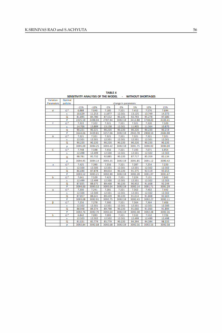
10 SENSITIVITY ANALYSIS OF THE MODEL

The sensitivity analysis is carried to explore the effect of changes in model parameters and costs on the optimal

policies, by varying each parameter (-15%,-10%,-5%, 0%, 5%, 10%, 15%) at a time for the model under study. The

results are presented in Table 4.

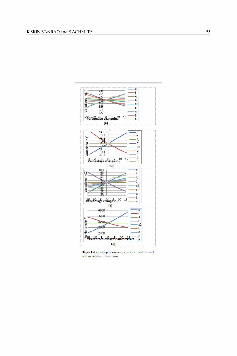
As the demand parameter d decreases, the optimal value of t1∗, the optimal selling price s∗, the optimal ordering

quantity Q* and profit rate are decreasing. If ‘d’ increases, the optimal value of t1∗, the optimal selling price s∗, the

optimal ordering quantity Q* and profit rate are increasing. If ‘f’ decreases, the optimal value of t1∗, the optimal

selling price s∗, the optimal ordering quantity Q* and profit rate are increasing. As ‘f’ increases, the optimal value

of t1∗, the optimal selling price s∗, the optimal ordering quantity Q* and profit rate are decreasing.

As the ordering cost ‘A’ decreases, the optimal value of t1∗, the optimal selling price s∗, the optimal ordering

quantity Q* remain constant and profit rate is increasing. If ‘A’ increases, the optimal value of t1∗, the optimal

selling price s∗, the optimal ordering quantity Q* remain constant and profit rate is decreasing. When the cost per

unit ‘C’ is decreasing, the optimal value of t1∗, the optimal

ordering quantity Q* and profit rate are increasing and the optimal selling price s∗ is decreasing. If ‘C’ is increas-

ing, the optimal value of t1∗, the optimal ordering quantity Q* and profit rate are decreasing. The optimal selling

price s∗ is increasing.

As the Production parameters ‘a’ decreases, the optimal value of t1∗ and profit rate are increasing, the optimal

selling price s∗ and the optimal ordering quantity Q* are decreasing. If ‘a’ increases, the optimal value of t1∗, and

profit rate are decreasing, the optimal selling price s∗and the optimal ordering quantity Q* are increasing. If ‘b’

decreases, the optimal value of t1∗ and the profit rate are increasing. The optimal ordering quantity Q* and the

optimal selling price s∗ are decreasing. If ‘b’ increases, the optimal value of t1∗ and profit rate are decreasing, the

optimal selling price s∗, the optimal ordering quantity Q* are increasing.

When the deteriorating parameters ‘a’ decreases, the optimal value of t1∗, the optimal ordering quantity Q*, the

optimal selling price s∗ are decreasing and the profit rate is increasing. If ‘a’ increases, the optimal value of t1∗,

the optimal ordering quantity Q*, the optimal selling price s∗ are increasing, and the profit rate is decreasing. If

‘b’ decreases, the optimal value of t1∗, the optimal ordering quantity Q*are decreasing. The optimal selling price

s∗ and profit rate are increasing. If ‘b’ increases, the optimal value of t1∗, the optimal ordering quantity Q* are

increasing, the optimal selling price s∗ and profit rate are decreasing. As the holding cost per unit ‘h’ decreases,

the optimal value of t1∗, the optimal ordering quantity Q* are decreasing, the optimal selling price s∗ and profit

rate are increasing. If ‘h’ increases, the optimal value of t1∗, the optimal ordering quantity Q* are increasing, the

optimal selling price s∗ and profit rate are decreasing.


11 CONCLUSIONS

In this paper, an economic production quantity model for deteriorating items is developed and analyzed. Here,

the replenishment (production) is time dependent. This production rate includes constant/increasing/ decreas-

ing rates of production for different values of the parameter. It is considered that the lifetime of the commodity

is finite and depends on time. The deterioration is a linear function of time. This rate of deterioration includes

constant/increasing/ decreasing rates of deterioration for different values of the parameter. It is supposed that

the demand is a function of the selling price. Supposing that the shortages are allowed and fully backlogged, the

instantaneous state of inventory, the stock loss due to deterioration, the backlogged demand and shortage levels

are obtained. With suitable cost considerations, the total profit rate function is obtained. By maximizing, the total

profit rate function, the optimal values of production downtime, production uptime, selling price and optimal

ordering quantity are derived. This model is extended to the case of without shortages. Results are illustrated

numerically and sensitivity analysis is carried out with respect to parameters in both the models. In a model with

shortages, the production rate parameters influence all the parameters except optimal ordering quantity. In the

model without shortages, the production rate parameters have a significant influence on the optimal values of

production schedule and profit. It is also seen that in both models the optimal values of production uptime and

total profit are highly sensitive to the production rate parameters and cost per unit time. Here, it is considered

when a single product is produced. For future scope, it is anticipated to extend the proposed model by consider-

ing the multi-commodity EPQ models with time dependent production and deterioration.

REFERENCES

[1]. Mak (1982). A Production lot size inventory model for deteriorating items, Computers & Industrial Engineer-

ing, Vol.6, No.4, pp 309- 317.

[2]. Chowdhary and Chaudari (1983). An order l evel inventory model for deteriorating items with a finite rate of

replenishment, Opsearch, Vol.20, pp.99-106.

[3]. Su, Lin, and Tsai (1999). A deterministic production inventory model for deteriorating items with an expo-

nential declining demand, OPSEARCH, Vol.36, No.2, pp 95-105.

[4.] Mandal and Phaujdar (1989). An inventory model for deteriorating items and Stock- dependent Consumption

Rate, Journal of Operational Research Society, Vol. 40, No. 5, pp 483-488.

[5.] Sujit and Goswami (2001). A replenishment policy for items with finite production rate and Fuzzy deteriora-

tion rate, Opsearch, Vol.38, No.4, pp 419.

[6]. Sana, Goyal, and Chaudhuri (2004). A production-inventory model for a deteriorating item with trended

demand and shortages, European Journal of Operational Research, Vol.157, No.2, pp 357-371.

[7]. Balkhi (2001). On a finite horizon production lot size inventory model for deteriorating items, European

Journal of Operational Research Vol. 132, No.1, pp 210-223.

[8] Samanta and Ajanta Roy (2004). A Deterministic Inventory Model of Deteriorating Items with Two rates of

production and Shortages, Tamsui Oxford Journal of Mathematics Sciences, Vol. 20, No.2, pp 205-218.

[9]. Lin, Gong, and Dah-Chuan (2006). On a production-inventory system of deteriorating items subject to random


machine breakdowns with a fixed repair time, Mathematical and computer modelling, Vol.43, No. 7-9, pp 920-932.

[10]. Chen and Chen (2008). Optimal pricing and replenishment schedule for deteriorating items over a finite

planning horizon, International Journal of Revenue Management, Vol.2, No. 3, pp 215-233.

[11]. Mirzazadeh, Seyyed Esfahani and Ghomi (2009). An inventory model under certain inflationary conditions,

finite production rate, and inflation –Dependent demand rate for deteriorating items with shortages, International

Journal of System Sciences, Vol.40, No.1, pp 21-31.

[12] .Manna and Chiang (2010). Economic production quantity models for deteriorating items with ramp type

demand, International Journal of Operational Research, Vol. 7, No. 4, pp 429-444.

[13]. Sridevi, Nirupama Devi and Srinivasa Rao (2010). An inventory model for deteriorating items with Weibull

rate of replenishment and selling price dependent Demand, International Journal of Operational research, Vol.9,

No.3, pp 329-349.

[14]. Tripathy, Pardhan, and Mishra (2010). An EPQ model for Linear deteriorating Item with Variable Holding

Cost, International Journal of Computational and Applied Mathematics, Vol.5 No. 2, pp 209-215.

[15]. Manna and Chiang (2010). Economic production quantity models for deteriorating items with ramp type

demand, International Journal of Operational Research, Vol. 7, No. 4, pp 429-444.

[16]. Sarkar and Moon (2011). An EPQ model with inflation in an imperfect production system, Applied Mathe-

matics, and Computation, Vol. 217, pp 6159- 6167.

[17]. Srinivasa Rao and Essey Kebede Muluneh (2012). Inventory models for deteriorating items with stock-

dependent production rate and Weibull decay, International Journal of Mathematical Archive- Vol.3, No.10, 2012,

pp.3709-3723. Available online through www.ijma.info ISSN 2229 – 5046.

[18]. Palanivel & Uthayakumar (2013). An EPQ model for deteriorating items with variable production cost, time

dependent holding cost and partial backlogging under inflation. OPSEARCH, Application Article, First Online:

28 December 2013, DOI: 10.1007/s12597- 013-0168-8.

[19]. Hui-Ming Teng (2013). EPQ models for deteriorating items with linearly discounted, back ordering under

limited utilization of facility Vol.7 No.29, pp 2882-2889, 7 August 2013, DOI: 10.5897/AJBM12.1214, ISSN 1993-

8233 c© 2013 Academic Journals, http://www.academicjournals.org/AJBM.

[20]. Sanjay Sharma and Singh (2013). EPQ Model of Deteriorating Inventory with Exponential Demand Rate

under Limited Storage, Africa Development and Resources Research Institute (ADRRI) Journal (www.adrri.org)

ISSN: 2343-6662 Vol. I, No.1, pp 23-31, October 2013.

[21]. Ashendra Kumar Saxena and Ravish Kumar Yadav (2013). An Optimal Production Cycle for Non- Instanta-

neous Deteriorating Items in Which Holding Cost Varies Quadratic in Time. International Journal of Application

or Innovation in Engineering & Management (IJAIEM), Web Site:www.ijaiem.org, Volume 2, No. 6, June 2013,

Page 148 -153, ISSN 2319 –4847.

[22]. Srinivasa Rao, Srinivasa Rao, Kesava Rao (2013). On Optimal Production Scheduling of an EPQ Model with

Stock Dependent Production Rate and Pareto Decay, Int. Journal of Applied Sciences and Engineering Research,

Vol. 2, Issue 3, 2013, ISSN 2277 – 9442.

[23]. Meenakshi Srivastava & Ranjana Gupta (2013). An EPQ model for deteriorating items with time and price

dependent demand under markdown policy, OPSEARCH (Jan–Mar 2014), Vol.51, No.1, pp.148–158.


[24]. Da Wen, Pan Ershun, Wang Ying and Liao Wenzhu (2014). An economic production quantity model for

a deteriorating system integrated with predictive maintenance strategy, Journal of Intelligent Manufacturing

c©Springer Science + Business Media New York 2014, 10.1007/s10845-014-0954-z.

[25]. Palanivel & Uthayakumar (2014). An EPQ model with variable production, probabilistic deterioration and

partial backlogging under inflation, Journal of Management Analytics, Vol.1,issue.3,DOI:10.1080/23270012.2014.971889,

published online: 30 Oct 2014.

[26]. Himani Dem, Singh and Jitendra Kumar (2014). An EPQ model with trapezoidal demand under volume

flexibility, International Journal of Industrial Engineering Computations, Volume 5 No 1, pp. 127-138, ISSN 1923-

2934 (Online) - ISSN 1923-2926 (Print) Quarterly Publication.

[27]. Ankit Bhojak, Gothi (2015), EPQ Model with Time-Dependent IHC and Weibull Distributed Deterioration

under Shortages, International Journal of Innovative Research in Science, Engineering and Technology (An ISO

3297: 2007 Certified Organization) Vol. 4, Issue 11, November, 2015, ISSN(Online): 2319- 8753,ISSN (Print): 2347-

6710

[28]. Kirtan Parmar and Gothi (2015), EPQ model for deteriorating items under three- parameter Weibull dis-

tribution and time dependent IHC with shortages. American Journal of Engineering Research (AJER) e- ISSN:

2320-0847 p-ISSN: 2320-0936 Volume- 4, Issue-7, pp-246-255.

[29]. Anitha, Parvathi(2016), An EPQ Model for Deteriorating Items with Time-Dependent Demand with Reliabil-

ity and Flexibility in a Fuzzy Environment International Journal of Innovative Research in Computer and Com-

munication Engineering An ISO 3297: 2007 Certified Organization, Vol. 4, Issue 2, February 2016. ISSN(Online):

2320-9801,ISSN (Print): 2320-9798.

[30]. Kousar Jaha Begum and P.Devendra(2016). E.P.Q Model for Deteriorating Items with Generalizes Pareto De-

cay Having Selling Price and Time-Dependent Demand, Research Journal of Mathematical and Statistical Sciences

Vol. 4(??), Page No: 1-11, February 2016, E-ISSN 2320–6047.

[31]. Dhir Singh & Singh(2017).Development of an EPQ Model for Deteriorating Product with Stock and Demand

Dependent Production rate under Variable Carrying Cost and Partial Backlogging, Volume: 5 Issue: 5, pp:478 –

497, ISSN: 2321-8169, IJRITCC |May 2017, Available @ http://www.ijritcc.org

[32]. Khedlekar, Namedeo, Nigwal (2018), Production-Inventory Model With Disruption Considering Shortage

And Time Proportional Demand. Yugoslav Journal of Operations Research, Vol. 28 (2018), Number 1, pp-123-139,

DOI:https://doi.org/10.2298/YJOR161118008K

[33]. Nitashah and Chetansinh Vaghela(2018), An epq model for deteriorating items with price dependent de-

mand and two level trade credit financing, revista investigacion operacional vol. 39, no. 2,pp: 170-180, 2018






Documents

ON OPTIMAL OPERATING POLICIES OF EPQ MODEL WITH TIME ... fileinventory model for deteriorating items over a ﬁnite planning horizon and a linear time-varying demand with a ﬁnite