Embed Size (px)
Citation preview

On Mixture Models in High-Dimensional Testing
for the Detection of Differential Gene Expression
Geoff McLachlan
Department of Mathematics & Institute for Molecular BioscienceUniversity of Queensland
ARC Centre of Excellence in Bioinformatics
http://www.maths.uq.edu.au/~gjm

Sample 1 Sample 2 Sample M
Gene 1Gene 2
Gene N
Expression ProfileE
xpression S
ignature
Microarray Data represented as N x M Matrix
N rows (genes) ~ 104
M columns (samples) ~ 102

Microarrays present new problems for statistics because the data are very high dimensional with very little replication.
The Challenge for Statistical Analysis of Microarray Data
The challenge is to extract useful information and discover knowledge from the data, such as gene functions, gene interactions, regulatory pathways, metabolic pathways etc.

Detection of Differential Expression
• Supervised Classification of Tissue Samples
• Clustering of Gene Profiles
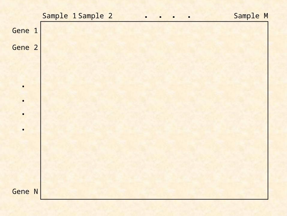
Gene 1
Gene 2
Gene N
.
.
.
.. . . .Sample 1 Sample 2 Sample M
Gene 1
Gene 2
Gene N
.
.
.
.. . . .Sample 1 Sample 2 Sample M
Class 1 Class 2

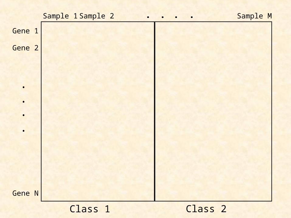
Hedenfalk Breast Cancer Data
• cDNA arrays, tumour samples from carriers of either the BRCA1 or BRCA2 mutation (hereditary breast cancers)
• BRCA1/BRCA2 mutations associated with decreased ability for DNA repair, yet pathologically distinct
• Dataset of M = 15 patients: 7 BRCA1 vs 8 BRCA2, with N = 3,226 genes.
The problem is to find genes which are differentially expressed between the BRCA1 and BRCA2 patients.
Hedenfalk et al. (2001) NEJM, 344, 539-547
An example of a gene from Hedenfalk et al (2001) breast cancer data
5066.0,1203.01002.0,3173.0 222
211 sxsx
3190.02 js
6739.021
11
21
nnj
jjj
s
xxt
512.0|)|(2 13 jj tFP
-0.587 -0.5 -0.0707 -0.265 -0.542 -0.522 0.265 -0.7 0.377 0.0318 -0.475 -0.627 -0.56 1.39 -0.4
Class 1 BRCA1: n1 = 7 tissues
Class 2BRCA2: n2 = 8 tissues
gene j

Sample 1 Sample M. . . . . . .
Gene 1
. . .
. . .
.
Gene N
Class 1(good prognosis)
Class 2(poor prognosis)
Supervised Classification (Two Classes)

Selection Bias
Bias that occurs when a subset of the variables is selected (dimension reduction) in some “optimal” way, and then the predictive capability of this subset is assessed in the usual way; i.e. using an ordinary measure for a set of variables.

Selection Bias
Discriminant Analysis:McLachlan (1992 & 2004, Wiley, Chapter 12)
Regression:Breiman (1992, JASA)
“This usage (i.e. use of residual of SS’s etc.) has long been a quiet scandal in the statistical community.”

Selection bias with SVM using RFE: GUYON, WESTON, BARNHILL & VAPNIK (2002, Machine Learning)
“The success of the RFE indicates that RFE has a built in regularization mechanism that we do not understand yet that prevents overfitting the training data in its selection of gene subsets.”
Ambroise, C. and McLachlan, G.J (2008). Selection bias in gene extraction on the basis of microarray gene-expression data.
Proceedings of the National Academy of Sciences USA 99, 6562-6566.

Figure 1: Error rates of the SVM rule with RFE procedure averaged over 50 random splits of colon tissue samples

Nature Reviews Cancer, Feb. 2005

Number of Genes Error Rate for Top 70 Genes (without correction for Selection Bias as Top 70)
Error Rate for Top 70 Genes (with correction for Selection Bias as Top 70)
Error Rate for 5422 Genes
1 0.40 0.40 0.40
2 0.31 0.37 0.40
4 0.24 0.40 0.42
8 0.23 0.32 0.29
16 0.22 0.33 0.38
32 0.19 0.35 0.38
64 0.23 0.32 0.33
70 0.23 0.32 -
128 - - 0.32
256 - - 0.29
512 - - 0.31
1024 - - 0.32
2048 - - 0.35
4096 - - 0.37
5422 - - 0.37
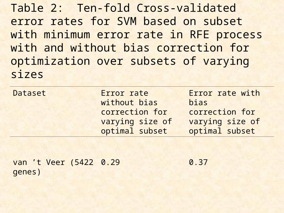
Table 2: Ten-fold Cross-validated error rates for SVM based on subset with minimum error rate in RFE process with and without bias correction for optimization over subsets of varying sizes
Dataset Error rate without biascorrection for varying size of optimal subset
Error rate with biascorrection for varying size of optimal subset
van ’t Veer (5422 genes) 0.29 0.37

Analysis of Breast Cancer Data• van’t Veer et al. (2002, Nature)• van de Vijver et al. (2002, NEJM)
FDA has approved on 7/2/07 a new genetic test called MammaPrint®, "that determines the likelihood of breast cancer returning within five to 10 years after a woman's initial cancer." According to the FDA, the test, a product of Agendia (Amsterdam, the Netherlands), is the first cleared product that profiles genetic activity.
MINDACT (Microarray for Node Negative Disease may Avoid Chemotherapy) prospective project, run by the EORTC (European Organisation for Research and Treatment of Cancer) and TRANSBIG, the translational research network of the Breast International Group

• Zhu, J.X., McLachlan, G.J., Ben-Tovim, L., and Wood, I. (2008). On selection biases with prediction rules formed from gene expression data. Journal of Statistical Planning and Inference 38, 374-386.
• McLachlan, G.J., Chevelu, J., and Zhu, J. (2008). Correcting for selection bias via cross-validation in the classification of microarray data. In Beyond Parametrics in Interdisciplinary Research: Festschrift in Honour of Professor Pranab K. Sen, N. Balakrishnan, E. Pena, and M.J. Silvapulle (Eds.). Hayward, California: IMS Collections, pp. 383-395.

Detection of Differential Expression
• Supervised Classification of Tissue Samples
• Clustering of Gene Profiles

Sample 1 Sample 2 Sample M
Gene 1Gene 2
Gene N
Expression ProfileE
xpression S
ignature
Microarray Data represented as N x M Matrix
N rows (genes) ~ 104
M columns (samples) ~ 102
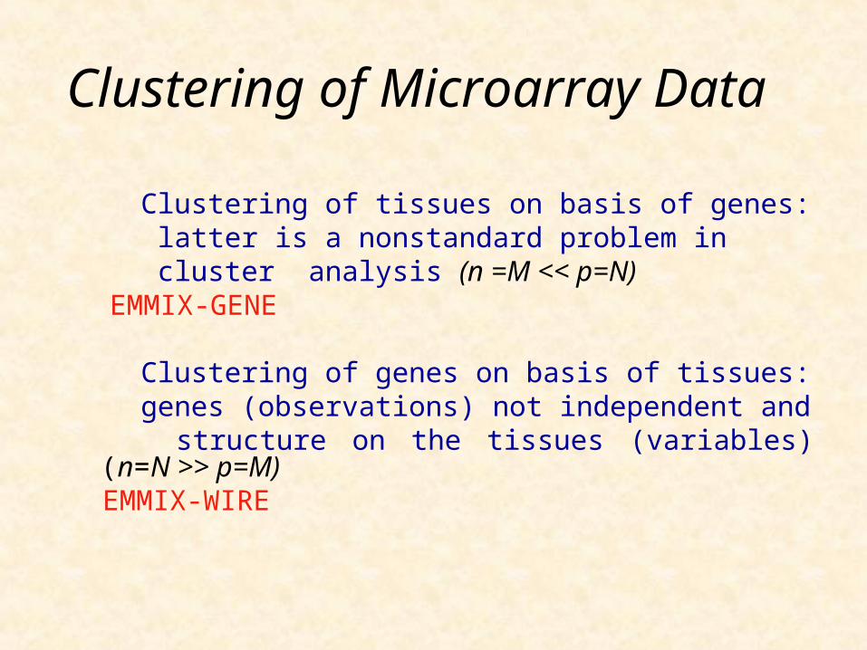
Clustering of Microarray Data
Clustering of tissues on basis of genes: latter is a nonstandard problem in cluster analysis (n =M << p=N) EMMIX-GENE
Clustering of genes on basis of tissues: genes (observations) not independent and structure on the tissues (variables) (n=N >> p=M) EMMIX-WIRE

• Longitudinal (with or without replication, for example time-course)
• Cross-sectional data
Clustering of gene expression profiles
Ng, McLachlan, Wang, Ben-Tovim Jones, and Ng (2006, Bioinformatics)
Supplementary information :
http://www.maths.uq.edu.au/~gjm/bioinf0602_supp.pdf
EMMIX-WIREEM-based MIXture analysis With Random Effects

),,1( njijiijij εVcUbXβy
In the ith component of the mixture, the profile vector yj for the jth gene follows the model
1p 1m 1bq 1cq 1p
) ,(~bqij N H0b
),(~ ci cqi N I0c
),(~ iA0Nij
Tiqiiii e
),,(),diag( 221 φWφA
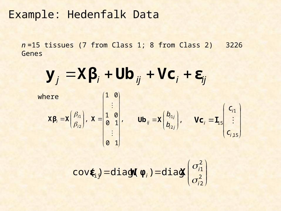
n =15 tissues (7 from Class 1; 8 from Class 2) 3226 Genes
ijiijij εVcUbXβy where
,
10
1001
01
,2
1
XXXβi
ii
,
2
1
ji
jiij b
bXUb
15,
1
15
i
i
i
c
c
IVc
22
21
ij diag)diag()cov(i
ii
XWφε
Example: Hedenfalk Data

• Flack, L.K. and McLachlan, G.J. (2008). Clustering methods for gene-expression data. In Handbook of Research on Systems Biology Applications in Medicine, A. Daskalaki (Ed.). Hershey, Pennsylvania: Information Science Reference. To appear.
• McLachlan, G.J., Bean, R., and Ng, S.K. (2008). Clustering of microarray data via mixture models. In Statistical Advances in Biomedical Sciences, A. Biswas, S. Datta, J. Fine, and M.R. Segal (Eds.). Hoboken, New Jersey: Wiley, pp. 365-384.
• McLachlan, G.J., Bean, R., and Ng, S.K. (2008). Clustering. In Bioinformatics, Vol. 2: Structure, Function, and Applications, J. Keith (Ed.). Totowa, New Jersey: Humana Press, pp. 423-439.

Gene 1
Gene 2
Gene N
.
.
.
.. . . .Sample 1 Sample 2 Sample M

Gene 1
Gene 2
Gene N
.
.
.
.. . . .Sample 1 Sample 2 Sample M
Class 1 Class 2

An example of a gene from Hedenfalk et al (2001) breast cancer data
5066.0,1203.01002.0,3173.0 222
211 sxsx
3190.02 js
6739.021
11
21
nnj
jjj
s
xxt
512.0|)|(2 13 jj tFP
-0.587 -0.5 -0.0707 -0.265 -0.542 -0.522 0.265 -0.7 0.377 0.0318 -0.475 -0.627 -0.56 1.39 -0.4
Class 1 BRCA1: n1 = 7 tissues
Class 2BRCA2: n2 = 8 tissues
gene j
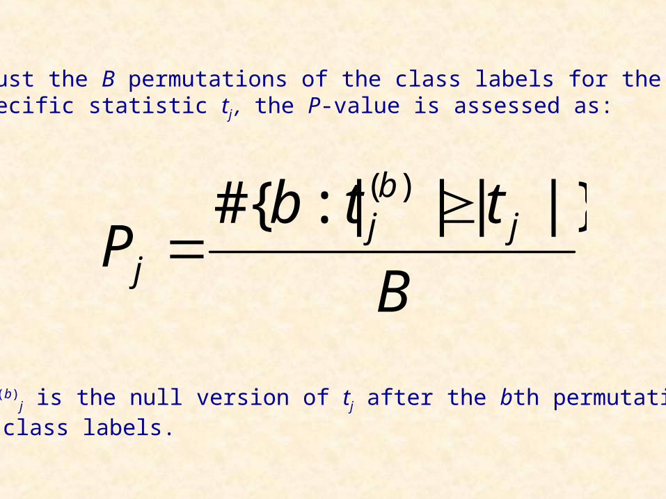
Using just the B permutations of the class labels for the gene-specific statistic tj , the P-value is assessed as:
where t(b)j is the null version of tj after the bth permutation
of the class labels.
B
ttbP j
bj
j
|}||:|{# )(

If we pool over all N genes, then:
B
b
jb
ij NB
NittiP
1
)( },...,1|,||:|{#

Multiplicity Problem
When many hypotheses are tested, the probability of a false positive increases sharply with the number of hypotheses.
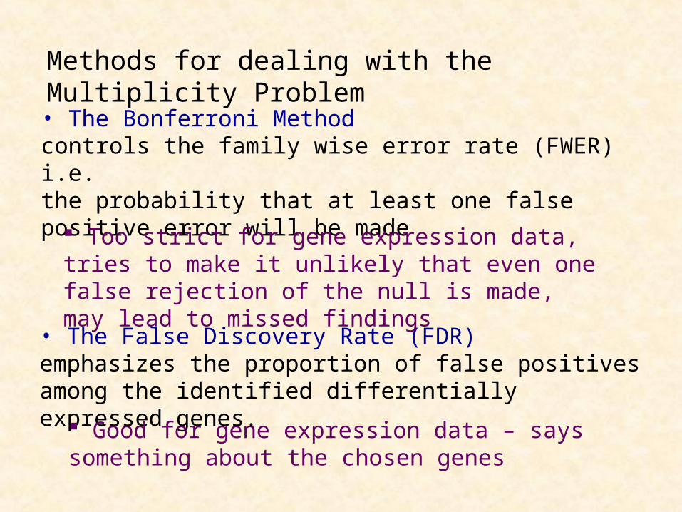
Methods for dealing with the Multiplicity Problem
• The Bonferroni Method controls the family wise error rate (FWER) i.e.the probability that at least one false positive error will be made
• The False Discovery Rate (FDR)emphasizes the proportion of false positives among the identified differentially expressed genes.
Too strict for gene expression data, tries to make it unlikely that even one false rejection of the null is made, may lead to missed findings
Good for gene expression data – says something about the chosen genes

TRUE
PREDICTED
Retain Null Reject Null
Null a b (false positive)
Non-null c (false negative) d
FDR ~ N
bFNDR ~
ca
c
The FDR and other error rates
r
Nr
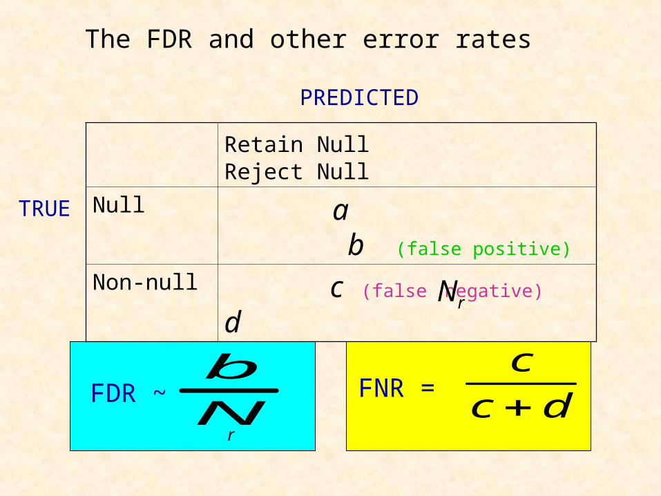
TRUE
PREDICTED
Retain Null Reject Null
Null a b (false positive)
Non-null c (false negative) d
FDR ~ N
b
Nr
FNR = dc
c
The FDR and other error rates
r

}1
{FDR
rNb
E
)1,max(1 rr NN where
}1)(
{FNDR
rNN
cE

|)|(2 13 jj tFP
)]([ 131
jj tFz

|)|(2 13 jj tFP
)1(1jj Pz

Local FDRLee (2000), Efron et al (2001), Newton et al. (2001) proposed a two-component mixture model
)()1()()( 1000 jjj zfzfzf
theorem)Bayes'(by )()1()(
)(
)(
)(
} | null is geneth {pr)(
1000
00
00
0
jj
j
j
j
jj
zfzf
zf
zf
zf
zjz

Global and Local FDR
• The global FDR is concerned with the average number of false positives among the selected genes.
• The local FDR gives a (probabilistic) assessment of differential expression for each gene.
An approach using mixture models gives estimates for the local FDR as well as the global FDR and other error rates such as FNR.
It also allows consideration whether an empirical null distribution should be adopted in place of the theoretical null.

• McLachlan GJ, Bean RW, Ben-Tovim Jones L, Zhu JX. (2005).Using mixture models to detect differentially expressed genes. Australian Journal of Experimental Agriculture 45, 859-866.
• McLachlan GJ, Bean RW, Ben-Tovim Jones L. (2006). A simple implentation of a normal mixture approach to differential gene expression in multiclass microarrays. Bioinformatics 26, 1608-1615.

• Efron B et al (2001) Empirical Bayes analysis of a microarray experiment. JASA 96,1151-1160.
• Efron B (2004) Large-scale simultaneous hypothesis testing: the choice of a null hypothesis. JASA 99, 96-104.
• Efron B (2004) Selection and estimation for large-Scale simultaneous inference.
• Efron B (2005) Local false discovery rates.• Efron B (2006) Correlation and large-scale
simultaneous significance testing.• Efron B (2006) Size, power and false discovery rates.
• Efron B (2007) Simultaneous inference: when should hypothesis testing problems be combined. http://www-stat.stanford.edu/~brad/papers/

F0: N(0,1), π0=0.9F1: N(1,1), π1=0.1
Reject H0 if z≥2
τ0(2) = 0.99972but FDR=0.17
F0: N(0,1), π0=0.6F1: N(1,1), π1=0.4
Reject H0 if z≥2
τ0(2) = 0.251but FDR=0.177
An example where local FDR is more informative: Glonek and Solomon (2003)
-4 -2 0 2 4
0.0
0.1
0.2
0.3
0.4
-4 -2 0 2 4
0.0
0.1
0.2
0.3
0.4
null
non-null
null
non-null

1. Obtain the z-score for each of the genes
The Procedure
2. Rank the genes on the basis of the z-scores, starting with the largest ones (the same ordering as with the P-values, Pj).
3. The posterior probability of non-differential expression of gene j, is given by 0(zj).
4. Conclude gene j to be differentially expressed if
0(zj) < c0
1jz jP1
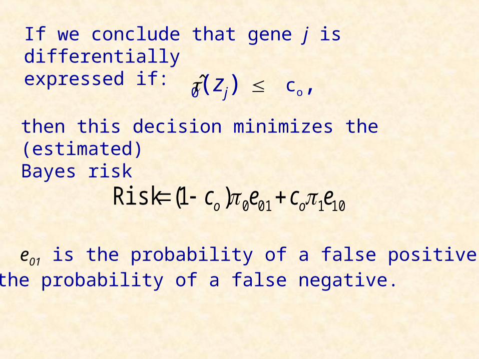
0(zj) co,
then this decision minimizes the (estimated) Bayes risk
If we conclude that gene j is differentially expressed if:
101010)1(Risk ecec oo
where e01 is the probability of a false positive and e10 is the probability of a false negative.

Suppose 0(z) is monotonic decreasing in z. Then
00 )(ˆ cz j for 0zz j
)(ˆ1
)(1ˆˆ
0
000
zF
zFRDF
00 |)( zzzE

Suppose 0(z) is monotonic decreasing in z. Then
for
)(ˆ1
)(1ˆˆ
0
000
zF
zFRDF
where )()( 000 zzF
1
101000
ˆ
ˆˆ)(ˆ)(ˆ
z
zzF
00 )(ˆ cz j 0zz j

For a desired control level , say = 0.05, define
)(ˆminarg0 zRDFzz
(1)
If)(ˆ1
)(1ˆ
00
zF
zF
is monotonic in z, then using (1)
to control the FDR [with and taken to be the empirical distribution function] is equivalent to using the Benjamini-Hochberg procedure based on the P-values corresponding to the statistic zj.
1ˆ 0 )(ˆ zF

)()1()(
)()(
1000
000
jj
jj zfzf
zfz
LOCAL FDR
(POSTERIOR) PROB. Of GENE j BEING NOT DIFFERENTIALLY EXPRESSED

)()1()(
)()(
1000
000
jj
jj zfzf
zfz
f0(zj)
N(0,1)
In order to proceed with estimation of π0 (can easilyestimate f(zj) from z1,…,zN) we need to make theproblem identifiable.
Now f0(zj) is N(0,1) and we have to assume somethingabout f1(zj).

)()1()(
)()(
1000
000
jj
jj zfzf
zfz
f0(zj)
f0(zj) f1(zj)
N(0,1)
N(0,1) N(μ1,σ12)

Z-values, null case Z-values, +1
Z-values, +2Z-values, +3

EMMIX-FDR
A program has been written in R which interfaces with EMMIX to implement the algorithm described in McLachlan et al. (2006).
We fit a mixture of two normal components
to the P-values of the test statistics calculated from the gene expression data.

Fit
via maximum likelihood.
For given π0, MLEs of μ1, σ12 are determined: try
various π0.
π0N(0,1) + (1- π0)N(μ1,σ12)

1100 ˆˆˆˆ z
21010
211
200
2 )ˆˆ(ˆˆˆˆˆˆ zs
When we equate the sample mean and varianceof the mixture to their population counterparts, we obtain:

)ˆ1/(ˆ 01 z
)ˆ1/(}ˆ)ˆ1(ˆˆ{ˆ 021000
221 zs
When we are working with the theoretical null,we can easily estimate the mean and varianceof the non-null component with the following formulae.

Estimated FDR
where
r
N
jjcj NzIzRDF
1
0],0[0 /))(ˆ()(ˆˆ0
N
jjcr zIN
10],0[ ))(ˆ(
0

N
jrjcj NNzIzRDFN
10),(1 )/())(ˆ()(ˆˆ
0
N
jj
N
jjcj zzIzRPF
10
10],0[0 )(ˆ/))(ˆ()(ˆˆ
0
N
jj
N
jjcj zzIzRNF
11
10),(1 )(ˆ/))(ˆ()(ˆˆ
0
Similarly, the false positive rate is given by
and the false non-discovery rate and false negativerate by:

-4 -2 0 2 4
05
01
00
15
0

Histogram of z-scores for 3226 Hedenfalk genes
z
Fre
qu
en
cy
-4 -2 0 2 4
02
04
06
08
01
00
Fitting two component mixture model to Hedenfalk data
Null
Non–Null(DE genes)

Gene j Pj zj 0 ( zj )
Gene 1
.
.
.
Gene 143
.
.
.
.
Gene 200
.
.
.
Gene N
0.0108
.
.
.
0.0998
0.1004
0.1010
.
.
0.1252
co = 0.1
Ranking and Selecting the Genes
FDR = Sum/143 = 0.06
Proportion ofFalse Negatives= 1 – Sum1/ 57= 0.89
Local FDR

co Nr
0.1 143 0.06 0.32 0.88 0.004
0.2 338 0.11 0.28 0.73 0.02
0.3 539 0.16 0.25 0.60 0.04
0.4 742 0.21 0.22 0.48 0.08
0.5 971 0.27 0.18 0.37 0.12
RDF ˆ DRNF ˆ RNF ˆ RPF ˆ
Estimated FDR and other error rates for various levelsof threshold co applied to the posterior probability of nondifferentialexpression for the breast cancer data (Nr=number of selected genes)

Storey and Tibshirani (2003) PNAS, 100, 9440-9445
Comparison of identified DE genes
Our method (143) Hedenfalk (175)
Storey and Tibshirani (160)
101
6
12
8
39
2924

Uniquely Identified Genes: Differentially Expressed between BRCA1 and BRCA2
Gene GO TermUBE2B, DDB2
(UBE2V1)
RAB9, RHOC
ITGB5, ITGA3
PRKCBP1
HDAC3, MIF
KIF5B, spindle body pole protein
CTCL1
TNAFIP1
HARS, HSD17B7
DNA repair
(cell cycle)
small GTPase signal transduction
integrin mediated signalling pathway
regulation of transcription
negative regulation of apoptosis
cytoskeleton organisation
vesicle mediated transport
cation transport
metabolism

Estimates of π0 for Hedenfalk data
• 0.52 (Broet, 2004)
• 0.64 (Gottardo, 2006)
• 0.61 (Ploner et al, 2006)
• 0.47 (Storey, 2002)
Using a theoretical null, we estimated π0 to be 0.65.

Theoretical and empirical nulls
Efron (2004) suggested the use of two kinds of null component: the theoretical and the empirical null. In the theoretical case the null component has mean 0 and variance 1 and the empirical null has unrestricted mean and variance.
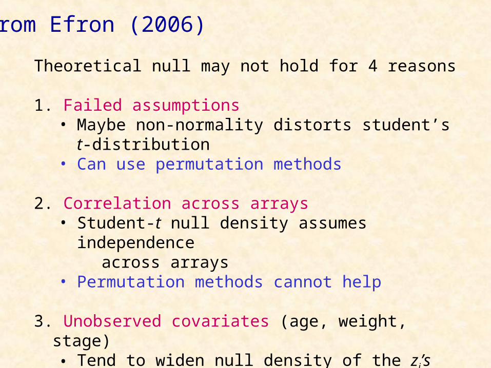
Theoretical null may not hold for 4 reasons
1. Failed assumptions• Maybe non-normality distorts student’s t-distribution• Can use permutation methods
2. Correlation across arrays• Student-t null density assumes independence
across arrays• Permutation methods cannot help
3. Unobserved covariates (age, weight, stage)• Tend to widen null density of the zj’s• Permutation methods cannot help
From Efron (2006)

4. Correlation across genes
Estimation of f(z) does not require independence of zj’s
)(ˆ/)()(ˆ 000 zfzfz jj

Suppose (1), (2), or (3) is applicable but (4) is not(assume genes independent).
null Zj may not be ~ N(0,1)
i.e. theoretical null may not hold
Thus: use empirical null

)()1()(
)()(
1000
000
jj
jj zfzf
zfz
μ0, σ02 are now estimated from the data.
Call N(μ0, σ02) the empirical null distribution.
f0(zj) f1(zj)f0(zj)
N(μ1,σ12)N(μ0,σ0
2)

Problem now is to fit
),()1(),( 2110
2000 NN
1. Specify an initial value of π0 (try theoretical null estimate and other estimates as before)
2. Rank zj’s and put Nπ0 smallest in nullcomponent and remainder in non-null component
3. Work out means/variances as if they are the truegroups

Can check for need of empirical null in placeof theoretical null by comparingtwice the increase in the log likelihoodwhen fitting μ0, σ0
2 instead offixing μ0=0 and σ0
2=1.
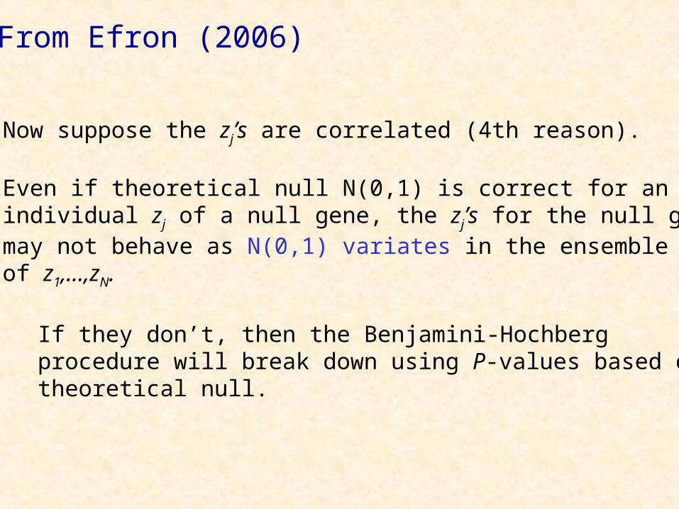
Now suppose the zj’s are correlated (4th reason).
Even if theoretical null N(0,1) is correct for anindividual zj of a null gene, the zj’s for the null genesmay not behave as N(0,1) variates in the ensembleof z1,…,zN.
If they don’t, then the Benjamini-Hochbergprocedure will break down using P-values based ontheoretical null.
From Efron (2006)

),()1(),( 2110
2000 NN
Fit
Still using maximum likelihood, although the function weare maximizing is no longer the true likelihood due to correlationacross the genes.
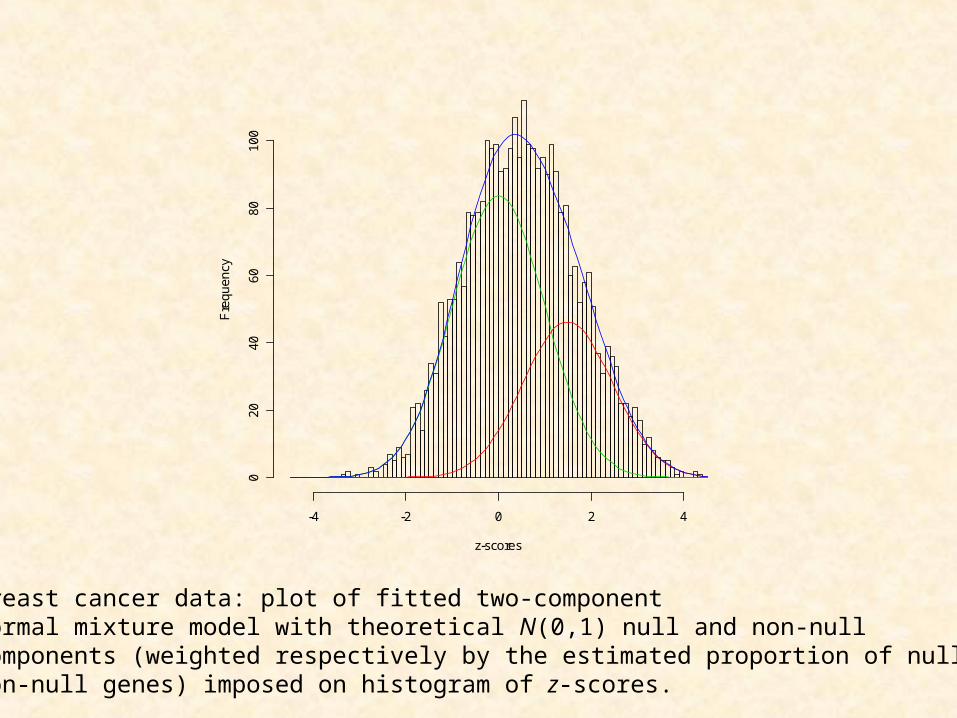
Breast cancer data: plot of fitted two-componentnormal mixture model with theoretical N(0,1) null and non-nullcomponents (weighted respectively by the estimated proportion of null andnon-null genes) imposed on histogram of z-scores.
z-scores
Fre
qu
en
cy
-4 -2 0 2 4
02
04
06
08
01
00

Hedenfalk breast cancer data:plot of fitted two-component normal mixture model with empirical nulland non-null components (weighted respectively by the estimated proportionof null and non-null genes) imposed on histogram of z-scores.
z-scores
Fre
qu
en
cy
-4 -2 0 2 4
02
04
06
08
01
00

co Nr
0.1 143 0.06 0.32 0.88 0.004
0.2 338 0.11 0.28 0.73 0.02
0.3 539 0.16 0.25 0.60 0.04
0.4 742 0.21 0.22 0.48 0.08
0.5 971 0.27 0.18 0.37 0.12
RDF ˆ DRNF ˆ RNF ˆ RPF ˆ
Table 1. Theoretical Null

co Nr
0.1 62 0.07 0.23 0.93 0.00
0.2 212 0.13 0.20 0.77 0.01
0.3 343 0.17 0.18 0.64 0.02
0.4 504 0.23 0.15 0.51 0.05
0.5 644 0.28 0.13 0.41 0.07
RDF ˆ DRNF ˆ RNF ˆ RPF ˆ
Table 2. Empirical Null

co Nr
0.1 143 0.06 0.32 0.88 0.004
62 0.07 0.23 0.93 0.00
0.2 338 0.11 0.28 0.73 0.02
212 0.13 0.20 0.77 0.01
RDF ˆ DRNF ˆ RNF ˆ RPF ˆ
Table 3. Theoretical versus Empirical Null

Allison et al. (2002) generated data for 10 mice over 3000 genes. The data are generated in six groups of 500 with a value ρ of 0, 0.4, or 0.8 in the off-diagonal elements of the 500 x 500 covariance matrix used to generate each group.
For a random 20% of the genes, a value d of 0, 4, or 8 is added to the gene expression levels of the last five mice.
Ben-Tovim Jones, L., Bean, R.W., McLachlan, G.J., and Zhu, J.X. (2006). Mixture models for detecting differentially expressed genes in microarrays. International Journal of Neural Systems 16, 353-362.
Allison Mice Simulation

Theoretical null, ρ=0.8, d=4

Empirical null, ρ=0.8, d=4
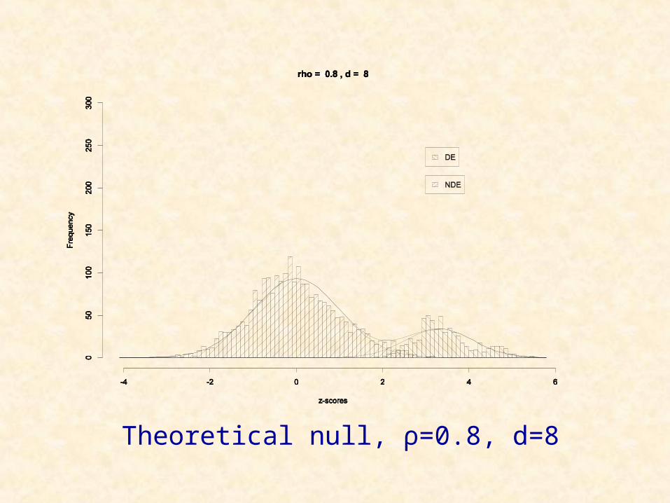
Theoretical null, ρ=0.8, d=8

Empirical null, ρ=0.8, d=8

• Longitudinal (with or without replication, for example time-course)
• Cross-sectional data
Clustering of gene expression profiles
Ng, McLachlan, Wang, Ben-Tovim Jones, and Ng (2006, Bioinformatics)
Supplementary information :
http://www.maths.uq.edu.au/~gjm/bioinf0602_supp.pdf
EMMIX-WIREEM-based MIXture analysis With Random Effects

n =15 tissues (7 from Class 1; 8 from Class 2) 3226 Genes
ijiijij εVcUbXβy where
,
10
1001
01
,2
1
XXXβi
ii
,
2
1
ji
jiij b
bXUb
15,
1
15
i
i
i
c
c
IVc
22
21
ij diag)diag()cov(i
ii
XWφε
Example: Hedenfalk Data
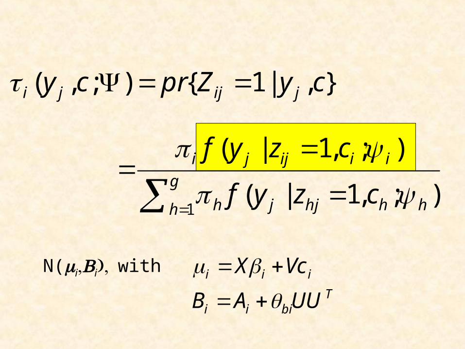
},|1{);,( cyZprcy jijji
g
h hhhjjh
iiijji
czyf
czyf
1);,1|(
);,1|(
N(iiwith iii VcX T
biii UUAB

co Nr
0.1 62 0.07 0.23 0.93 0.00
257 0.06 0.32 0.79 0.01
0.2 212 0.13 0.20 0.77 0.01
480 0.10 0.27 0.63 0.02
RDF ˆ DRNF ˆ RNF ˆ RPF ˆ
Table 4. Empirical versus Clustering Approach
Summary
• Mixture model based approach to finding DE genes is both convenient and effective
• Gives measure of local as well as global FDR; also gives other error rates
• Provides an empirical null for use when theoretical null may be misleading