On Linear Stability Analysis

of High-Order Finite-Difference Methods

David W. Zingg,∗ and Matthew Lederle†

Institute for Aerospace Studies, University of Toronto

4925 Dufferin St., Toronto, Ontario M3H 5T6, Canada

In order to produce the desired global order of accuracy, high-order finite-differencemethods require suitably accurate stable boundary schemes. Various tools can be helpfulin providing insight into the stability of numerical boundary schemes, including spectra,pseudospectra, and the singular value decomposition. In this paper, these tools are appliedto several different discretizations of the linear convection equation which display varioustypes of instability. Pseudospectra are seen to be a convenient and effective means ofdetecting instabilities. The same instabilities can also be revealed by either the spectrum orthe spectrum of the associated circulant matrix resulting from the assumption of periodicboundary conditions. Finally, the singular value decomposition is shown to be a goodindicator of the cause of the instability.

I. Introduction

One of the challenges in the development of high-order finite-difference discretizations is the need forstable boundary schemes of sufficient accuracy. For continuous hyperbolic problems, Nth-order global spatialaccuracy is achieved when the interior scheme is order N and the boundary schemes are of order (N − 1) orbetter.1 If the boundary schemes are of order lower than (N − 1), then the benefit of the high-order interiorscheme can be greatly reduced.

The challenge of developing boundary schemes for high-order finite-difference methods is compoundedby the complexity of proving Lax-Richtmyer stability for hyperbolic initial-boundary-value problems. Ap-plication of the normal mode analysis of Godunov and Ryabenkii2 and Gustafsson, Kreiss, and Sundstrom(GKS)3 to general high-order difference methods can be exceedingly difficult.4

Carpenter et al.5 and Zingg and Lomax6 developed stable boundary schemes for sixth-order compact andnoncompact interior schemes, respectively. These boundary operators were found in an ad hoc manner. Sub-sequently, efforts have concentrated on the development of more systematic approaches to the development ofstable boundary schemes using summation-by-parts energy norms5,7–10 and the simultaneous approximationterm method.11

Asymptotic stability is not a sufficient condition for Lax-Richtmyer stability. In other words, a semi-discrete finite-difference operator with eigenvalues within the stability region of the time integration methodis not necessarily stable; neither is a fully-discrete operator with eigenvalues within the unit circle. For non-normal matrices, the eigenvalue spectrum, while providing an accurate picture of the long-time asymptoticbehaviour, does not accurately describe the solution behaviour at finite time. For such matrices (andoperators) the pseudospectrum can provide a much more accurate picture. Reddy and Trefethen12 appliedpseudospectra to the stability analysis of finite-difference methods. The ability of pseudospectra to revealGKS instabilities is discussed in the recent book by Trefethen and Embree.13 The authors remark thatthe connection between pseudospectra and the stability of numerical boundary schemes has gone largelyunexploited; the sole published exception is a 1997 paper by Zingg.14

This paper is something of a sequel to the 1997 paper by the first author. That paper presented aconjecture that can be restated as the following question: Can a method be Cauchy stable (i.e. stable if

∗Professor, Senior Canada Research Chair in Computational Aerodynamics, 2004 Guggenheim Fellow, Senior AIAA Member.†Undergraduate Student

1 of 14

American Institute of Aeronautics and Astronautics

periodic boundary conditions are assumed) and asymptotically stable, but not Lax-Richtmyer stable? Theusefulness of the singular value decomposition in providing insight into instabilities was also demonstrated.The objective of the present paper is to explore these issues further, particularly in light of the examplesgiven by Trefethen and Embree13 showing the effectiveness of pseudoeigenvalues in revealing the existenceof unstable modes.

In the next section, the notation and stability definitions are introduced, and pseudospectra are defined.This is followed by five examples showing various types of instability, beginning with an instability associatedwith the numerical scheme at the inflow boundary. The second example gives stable inflow boundaryoperators, while the third example is a mild instability associated with the interior scheme. Examplesfour and five are unstable cases from Trefethen and Embree.13 The first is an explicit scheme, the second isimplicit. In both cases the instability is associated with the outflow boundary scheme.

II. Background

A. Model Problem and Notation

We consider the following initial-boundary-value problem (the linear convection equation):

∂U

∂t+

∂U

∂x= 0 (1)

on the domain 0 ≤ x ≤ 1. The initial condition is U(x, 0) = U0(x). This equation governs the propagationof a scalar, U(x, t), to the right with unit speed. The left boundary is called the inflow boundary, since ingeneral a time-varying boundary condition can be specified there, representing an incoming wave. In thestudy of stability, we need only consider the Dirichlet boundary condition U(0, t) = 0. The right boundaryis called the outflow boundary. The wave leaves the domain through this boundary without reflection. Thisequation is a suitable representative model problem for hyperbolic systems.

The notation here parallels that in Lomax et al.15 The numerical approximation to U(x, t) is written as

unj ≈ U(j∆x, n∆t) (2)

where the domain is divided into M equal subintervals of length ∆x, and the time step ∆t = tn+1 − tn isalso constant. When a finite-difference approximation is applied to the spatial derivative in (1), the followingsystem of ordinary differential equations (ODE’s) is obtained:

du

dt= Au (3)

whereA =

1∆x

A (4)

andu = [u1, u2, . . . , uM ]T (5)

The matrix A is an M ×M matrix that is typically banded. If the same difference operator is used at eachnode in the interior of the grid, then the entries are constant along the bands, except for the first and last fewrows, i.e. A is a quasi-Toeplitz matrix. The entries in these rows are determined by the numerical boundaryschemes (NBS’s).

When a time integration method is applied to the system of ODE’s (3), the resulting difference equationcan be written in the form

vn+1 = Cvn (6)

where v is a vector of length M ′ and C is an M ′×M ′ matrix. The vector v contains the numerical solutionat all of the time levels required by the differencing scheme. For example, for a two-step time-marchingmethod, M ′ = 2M and

vn =

[un

un−1

](7)

where u is defined in (5). If a one-step time integration method is used, then M ′ = M and v = u. Notethat the fully-discrete form (6) always exists, while the semi-discrete form (3) exists only if the spatial andtemporal discretizations are performed separately.

2 of 14

American Institute of Aeronautics and Astronautics

B. Stability Definitions and Spectra

As a result of the Lax equivalence theorem, Lax-Richtmyer stability is the most fundamental definition ofstability. A difference approximation is Lax-Richtmyer stable if there exists a constant K ≥ 1 (independentof n) such that, for an arbitrary initial condition u0,

‖un‖ ≤ K‖u0‖ (8)

for all n ≥ 0, 0 ≤ n∆t ≤ T with T fixed. A necessary and sufficient condition for Lax-Richtmyer stability is

‖Cn‖ ≤ K (9)

for the same conditions as above, with C defined in (6).A necessary condition for stability is that the associated Cauchy problem (obtained by the assumption

of periodic boundary conditions) is stable. The assumption of periodic boundary conditions produces acirculant matrix, sometimes called the circulant cousin of the quasi-Toeplitz matrix which includes thenumerical boundary schemes.16 The Cauchy stability can be checked based on the spectrum of this circulantmatrix. This tests the stability of the interior scheme independent of the boundary schemes.

Another useful concept, although neither necessary nor sufficient for Lax-Richtmyer stability, is asymp-totic stability, which is the requirement that ||Cn|| remain bounded as n goes to infinity with fixed M ′.When consistent with the physics of the problem, the stronger condition that ||Cn|| tend to zero as n goesto infinity is a desirable property of a difference method. Since the solution of (1) tends to zero as t goes toinfinity when U(0, t) = 0, the stronger condition is appropriate for discretizations of (1). This leads to therequirement that

ρ(C) < 1 (10)

where ρ(C) is the spectral radius of C, i.e. all of the eigenvalues of C must lie within the unit circle in thecomplex plane.

For difference methods with an intermediate semi-discrete form, (10) is satisfied if all of the eigenvaluesof ∆tA lie within the stable region of the time integration scheme. The ODE system (3) is termed inherentlystable if the spectrum of A lies entirely in the left half-plane.15 The solution of the ODE’s then tends to zeroas t goes to infinity.

C. Non-Normal Matrices and Pseudospectra

If C is a normal matrix,a then its eigenvalue spectrum gives an accurate picture of its behaviour. Thespectral radius is equal to the L2 norm, and the spectral radius condition (10) is sufficient for stability. If weassume that C is nondefective, then the following relation holds between the matrix norms ||Cn|| and theeigenvalues Λn:

||Cn|| = ||XΛnX−1|| ≤ ||X|| · ||X−1|| · ||Λn|| = κ(X)||Λn|| (11)

where X is the matrix of eigenvectors of C, Λ the diagonal matrix of eigenvalues, and κ(X) is the conditionnumber of X. The relationship depends upon the condition number of the eigenvector matrix. For a normalmatrix, the eigenvectors are orthogonal, and the condition number is unity.

For a non-normal matrix the eigenvectors can be far from orthogonal, and the condition number can belarge. Therefore, even though the eigenvalue spectrum still describes the asymptotic behaviour accurately,||Cn|| can far exceed ||Λn||. If the spectral radius of C is less than unity, then ||Cn|| must tend to zero as ngoes to infinity but can grow arbitrarily large for finite n. For nondefective C, we can write the solution to(6) as follows:15

vn =M∑

m=1

cm(σm)nxm (12)

where σm and xm are the eigenvalues and eigenvectors of C. The coefficients cm are determined from theinitial condition, i.e. the initial condition is decomposed into a linear combination of the eigenvectors. Ifρ(C) < 1, (12) shows that each eigenvector component of the solution must decay with increasing n. Thenorm of the solution can nevertheless increase because the eigenvectors are far from orthogonal. When aninitial condition is represented as a linear combination of eigenvector components, the coefficients can be

aThat is CC∗ = C∗C.

3 of 14

American Institute of Aeronautics and Astronautics

−0.1 −0.05 0 0.05−2

−1.5

−1

−0.5

0

0.5

1

1.5

2

λr

λ i

Figure 1. Eigenvalue spectra for sixth-order centered differences with conventional fifth-order inflow NBS (o)and stable fifth-order inflow NBS obtained with α = 3/20, β = 1/10 (x), M = 100.

very large. As the solution evolves, the cancellation needed to produce the initial condition is lost, and thenorm of the solution can grow.

Pseudospectra provide a more accurate picture of the behaviour of non-normal matrices and operators.They have been applied to a wide range of applications, most extensively by Trefethen and co-workers.Rather than providing a list of references, other than the paper by Reddy and Trefethen12 and the bookby Trefethen and Embree,13 we refer the reader to the Pseudospectra Gateway.17 This web site providesextensive information about pseudospectra, including definitions, theorems, a history, and a bibliography. Italso provides software for computing pseudospectra, such as the EigTool for MATLAB.18

There are several definitions of pseudospectra. The most relevant here is the following definition in termsof eigenvalues:17

Λε = {z ∈ C : z ∈ Λ(A + E) for some E with ||E|| ≤ ε} (13)

Therefore an eigenvalue of a perturbed matrix A + E, where E is a random matrix with norm ε, is anε-pseudo-eigenvalue of A. If the ε-pseudospectrum lies within ε of the spectrum, then the spectrum likelyprovides an accurate picture. If the deviation is significantly greater than ε, then the pseudospectrum likelyprovides a more accurate predictor of the behaviour of || exp(At)|| at finite t for the semi-discrete matrix Ain (3) and of ||Cn|| at finite n for the fully-discrete matrix C in (6).

III. Example 1: An Instability Related to the Inflow Boundary

We consider a spatial discretization of the linear convection equation using sixth-order centered differencesin the interior. In order to achieve sixth-order global accuracy, numerical boundary schemes of at least fifth-order are required. At the outflow boundary, fifth-order upwind and upwind-biased operators can be used.At the inflow boundary, fifth-order downwind-biased operators are a natural choice.

The spectrum of A with M = 100 is displayed in Figure 1. The criterion that all of the eigenvalues liein the left half-plane is clearly violated. As M tends to infinity, the eigenvalue spectrum of a quasi-Toeplitzmatrix can be partitioned into a boundary-condition independent spectrum and a boundary-condition de-pendent spectrum.16 The boundary condition independent spectrum is the spectrum of the Toeplitz matrixassociated with the auxiliary Dirichlet problem found by replacing all boundary conditions by homogeneousDirichlet boundary conditions. In the asymptotic limit, the spectrum of the auxiliary Dirichlet matrix isbounded by the spectrum of the circulant cousin associated with the Cauchy problem. If the Cauchy prob-lem is stable, any instabilities must thus be associated with the boundary-condition dependent spectrum,which is independent of the matrix size, and are related to the NBS’s.4 In our example, there exist twoboundary-condition dependent eigenvalues that lie in the right half-plane.

4 of 14

American Institute of Aeronautics and Astronautics

λr

λ i

−2 −1.5 −1 −0.5 0 0.5 1−2

−1.5

−1

−0.5

0

0.5

1

1.5

2

Figure 2. Spectrum (x) and pseudospectra for example 2 with M = 100.

IV. Example 2: Stable Inflow Boundary Schemes

Next we consider the modified inflow NBS developed by Zingg et al.6,19,20 The stencil of the operators atthe two grid nodes nearest the inflow boundary is increased by one element beyond that needed for fifth-orderaccuracy. This results in the following two-parameter family of fifth-order inflow NBS’s:

(δxu)1 =1

60∆x[(−12 + 60α)u0 + (−65− 360α)u1 + (120 + 900α)u2

+(−60− 1200α)u3 + (20 + 900α)u4 + (−3− 360α)u5 + 60αu6] (14)

(δxu)2 =1

60∆x[(3 + 60β)u0 + (−30− 360β)u1 + (−20 + 900β)u2

+(60− 1200β)u3 + (−15 + 900β)u4 + (2− 360β)u5 + 60βu6] (15)

The spectrum obtained with α = 3/20, β = 1/10 is displayed in Figure 1. The entire spectrum lies inthe left half-plane. There are still two boundary-condition dependent eigenvalues, but they now lie well inthe left half-plane. Therefore, we have both Cauchy stability and asymptotic stability. Pseudospectra areshown in Figure 2. There are no bulges characteristic of instability. Hence we conclude that the scheme isLax-Richtmyer stable.

V. Example 3: A Mild Instability Related to the Interior Difference Operator

Next we consider a full discretization with a mild instability caused by the interior difference scheme.The spatial operator is given by sixth-order centered differences plus a symmetric operator given by

(δsxU)j =

1∆x

[d3 (Uj+3 + Uj−3) + d2 (Uj+2 + Uj−2) +d1 (Uj+1 + Uj−1) + d0Uj ] (16)

with d0 = 0.1, d1 = −0.0804523, d2 = 0.0403545, and d3 = −0.00990220. When applied to

dU

dt= f(U, t) (17)

the six-stage time-marching method is given by:19

5 of 14

American Institute of Aeronautics and Astronautics

λr

λi

−0.5 −0.4 −0.3 −0.2 −0.1 0 0.10

0.5

1

1.5

2

Figure 3. Spectra of A with periodic boundary conditions (o) and NBS’s (x) and the stability contour of thetime integration method (18) (—–).

U(1)n+α1

= Un + ∆tα1fn

U(2)n+α2

= Un + ∆tα2f(1)n+α1

U(3)n+α3

= Un + ∆tα3f(2)n+α2

(18)

U(4)n+α4

= Un + ∆tα4f(3)n+α3

U(5)n+α5

= Un + ∆tα5f(4)n+α4

Un+1 = Un + ∆tf(5)n+α5

where Un = U(tn), and

f(k)n+α = f(U (k)

n+α, tn + αh)

with α1 = 1/6, α2 = 1/5, α3 = 1/4, α4 = 1/3, α5 = 1/2.The NBS at the inflow boundary is as given in (14) and (15) with α = 3/20, β = 1/10. At the

outflow boundary, fifth-order upwind and upwind-biased operators are used. The matrix entries are givenin the Appendix. Figure 3 shows the stability contour of the time-marching method with a solid line. Theeigenvalues of the associated circulant matrix are shown by the symbol “o”. Some lie just outside the stableregion of the time-marching method (near the imaginary axis between 0.8 and 1.2). The eigenvalue spectrumof the spatial operator matrix with NBS’s and M = 100 is shown by the symbol “x”, demonstrating theasymptotic stability of the method for this value of M .

Figure 4 shows the pseudospectra for M = 5000. The bulge in the pseudospectra clearly reveals theinstability. In Zingg14 the matrix used was too small to reveal such a mild instability. The pseudospectraare clearly helpful in revealing the instability in this case, and the spectrum is not. However, the instabilityis also easily seen by consideration of the spectrum of the associated circulant operator, which can be foundanalytically.

VI. Example 4: An Instability Related to the Outflow Boundary:Explicit Scheme

Next we consider an example from Trefethen and Embree.13 In order to maintain consistency with theirnotation, we consider the linear convection equation with the direction of propagation reversed, i.e.

∂U

∂t=

∂U

∂x(19)

6 of 14

American Institute of Aeronautics and Astronautics

−0.05 −0.04 −0.03 −0.02 −0.01 0 0.01 0.02 0.03 0.04 0.050.8

0.85

0.9

0.95

1

1.05

1.1

1.15

1.2

1.25

1.3

1.35

λr

λ i

ε = 10−2

ε = 10−3

ε = 10−4

ε = 10−5

ε = 10−6

Figure 4. Pseudospectra for example 3 with M = 5000.

−1 −0.5 0 0.5 1−1

−0.5

0

0.5

1

λr

λ i

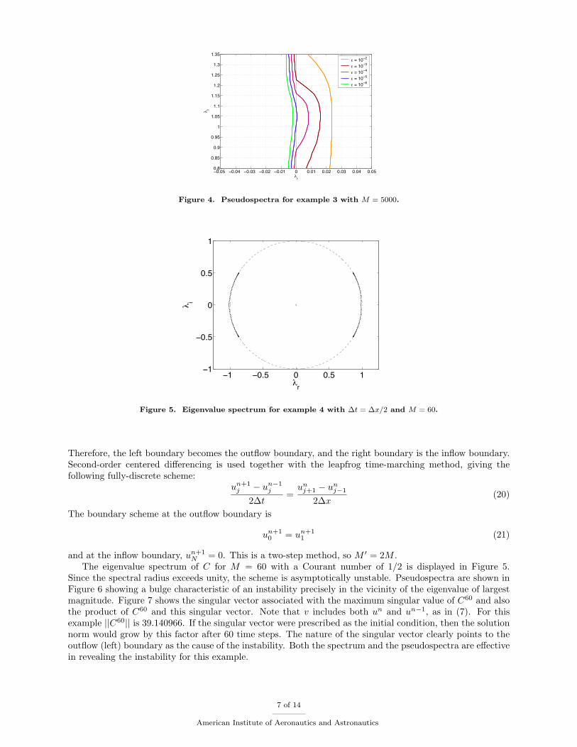
Figure 5. Eigenvalue spectrum for example 4 with ∆t = ∆x/2 and M = 60.

Therefore, the left boundary becomes the outflow boundary, and the right boundary is the inflow boundary.Second-order centered differencing is used together with the leapfrog time-marching method, giving thefollowing fully-discrete scheme:

un+1j − un−1

j

2∆t=

unj+1 − un

j−1

2∆x(20)

The boundary scheme at the outflow boundary is

un+10 = un+1

1 (21)

and at the inflow boundary, un+1N = 0. This is a two-step method, so M ′ = 2M .

The eigenvalue spectrum of C for M = 60 with a Courant number of 1/2 is displayed in Figure 5.Since the spectral radius exceeds unity, the scheme is asymptotically unstable. Pseudospectra are shown inFigure 6 showing a bulge characteristic of an instability precisely in the vicinity of the eigenvalue of largestmagnitude. Figure 7 shows the singular vector associated with the maximum singular value of C60 and alsothe product of C60 and this singular vector. Note that v includes both un and un−1, as in (7). For thisexample ||C60|| is 39.140966. If the singular vector were prescribed as the initial condition, then the solutionnorm would grow by this factor after 60 time steps. The nature of the singular vector clearly points to theoutflow (left) boundary as the cause of the instability. Both the spectrum and the pseudospectra are effectivein revealing the instability for this example.

7 of 14

American Institute of Aeronautics and Astronautics

−1 −0.5 0 0.5 1−1

−0.5

0

0.5

1

λr

λ i

Figure 6. Pseudospectra for example 4 with ∆t = ∆x/2 and M = 60.

0 20 40 60 80 100 120−8

−6

−4

−2

0

2

4

6

8

j (mesh index)

u j

Figure 7. Singular vector of C60 (· · ·) for example 4 and the product of C60 and this singular vector (—–).Note that the singular vector has been amplified by a factor of ten.

VII. Example 5: An Instability Related to the Outflow Boundary:Implicit Scheme

This example is an unstable implicit scheme from Trefethen and Embree.13 The spatial discretizationis again second-order centered differences, but the time-marching method is the trapezoidal method.15 Thefully-discrete scheme is given by

un+1j − un

j

∆t=

unj+1 − un

j−1

4∆x+

un+1j+1 − un+1

j−1

4∆x(22)

The boundary scheme at the outflow boundary is

un+10 = un

2 (23)

and at the inflow boundary, un+1N = 0. This is a one-step scheme, so M ′ = M .

8 of 14

American Institute of Aeronautics and Astronautics

−1 −0.5 0 0.5 1−1

−0.5

0

0.5

1

λr

λ i

Figure 8. Eigenvalue spectrum for example 5 with ∆t = ∆x/2 and M = 60.

100

102

104

106

108

0

2

4

6

8

10

12

14

n

||Cn ||

M=30M=60M=120

Figure 9. ||Cn|| vs. n for example 5 with ∆t = ∆x/2 and M = 30, 60, 120.

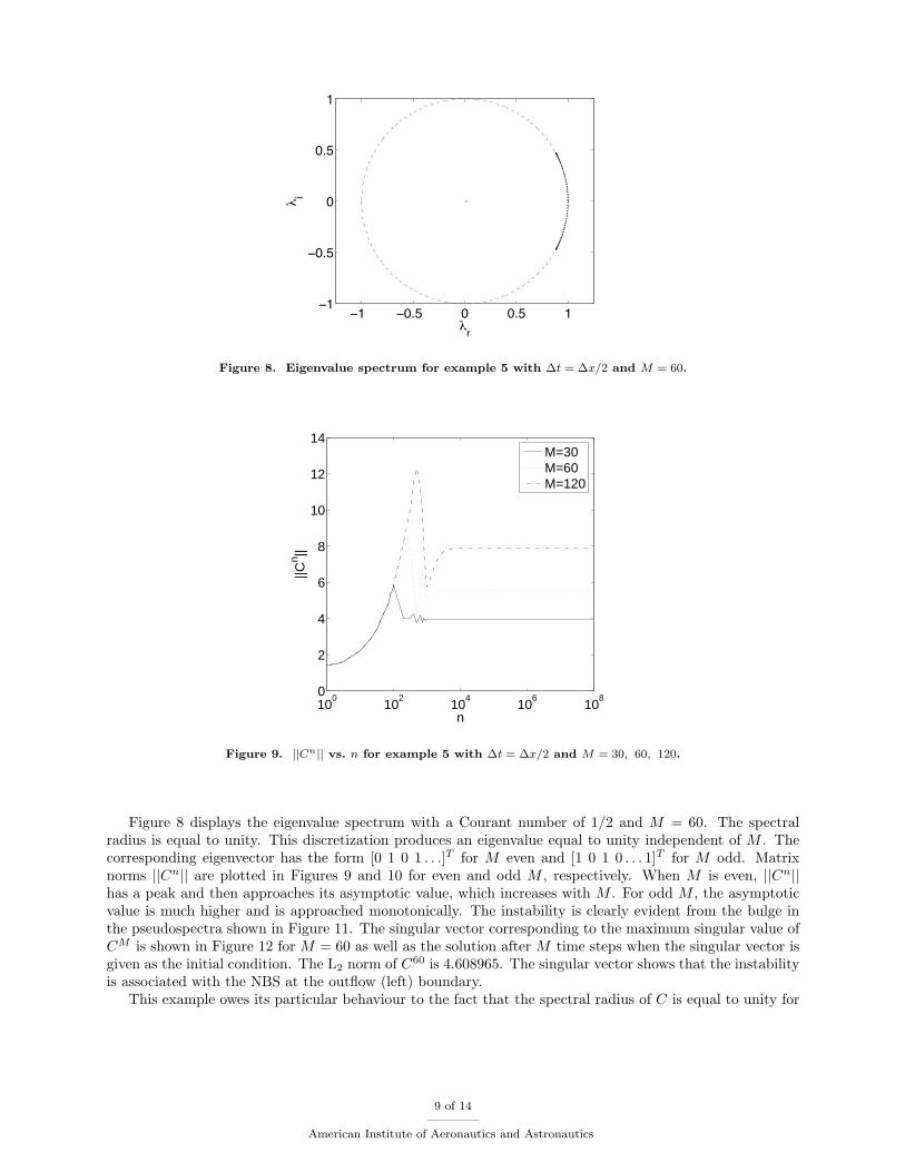
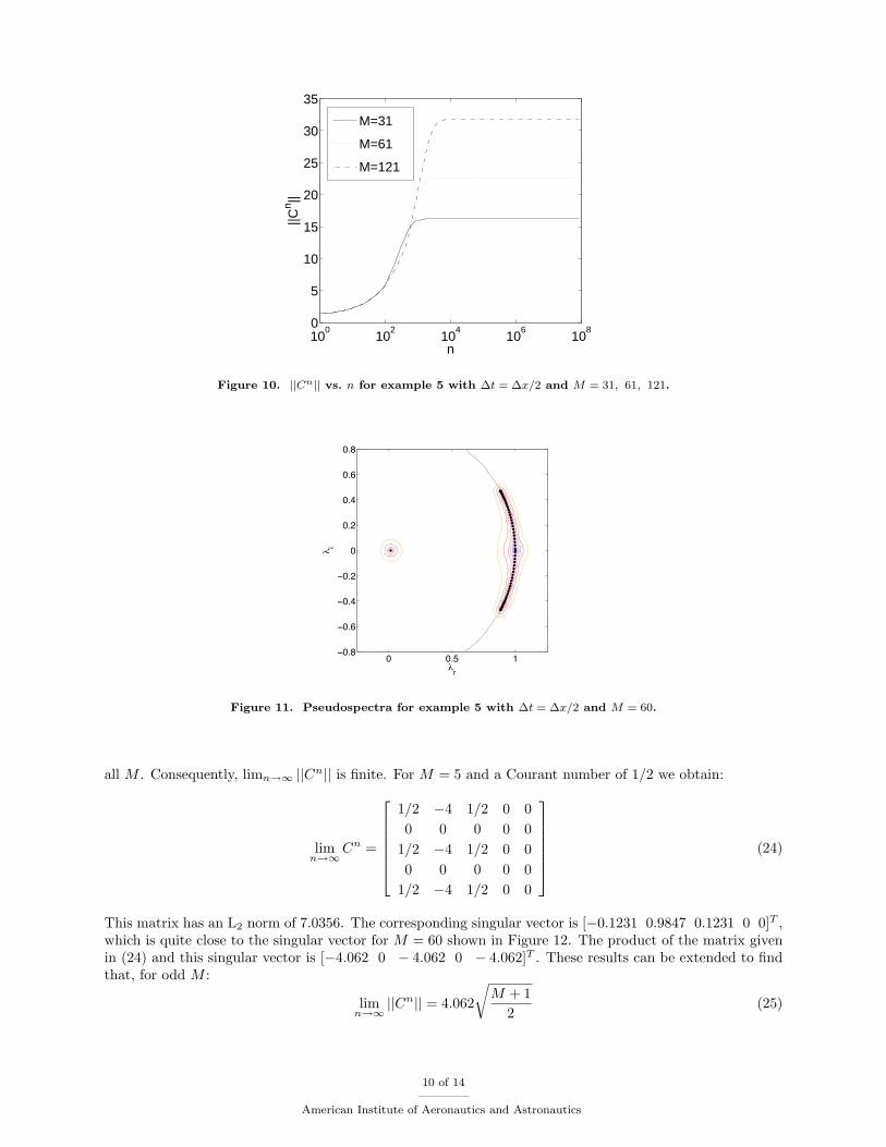
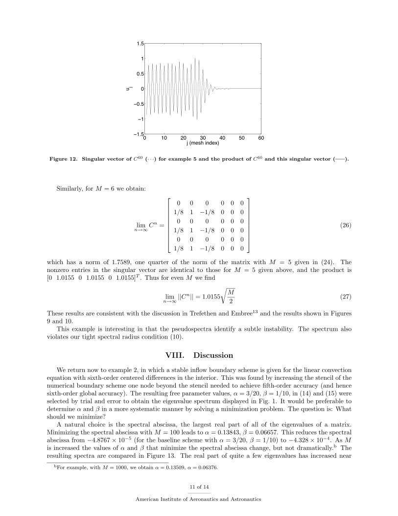
Figure 8 displays the eigenvalue spectrum with a Courant number of 1/2 and M = 60. The spectralradius is equal to unity. This discretization produces an eigenvalue equal to unity independent of M . Thecorresponding eigenvector has the form [0 1 0 1 . . .]T for M even and [1 0 1 0 . . . 1]T for M odd. Matrixnorms ||Cn|| are plotted in Figures 9 and 10 for even and odd M , respectively. When M is even, ||Cn||has a peak and then approaches its asymptotic value, which increases with M . For odd M , the asymptoticvalue is much higher and is approached monotonically. The instability is clearly evident from the bulge inthe pseudospectra shown in Figure 11. The singular vector corresponding to the maximum singular value ofCM is shown in Figure 12 for M = 60 as well as the solution after M time steps when the singular vector isgiven as the initial condition. The L2 norm of C60 is 4.608965. The singular vector shows that the instabilityis associated with the NBS at the outflow (left) boundary.

This example owes its particular behaviour to the fact that the spectral radius of C is equal to unity for

9 of 14

American Institute of Aeronautics and Astronautics

100

102

104

106

108

0

5

10

15

20

25

30

35

n

||Cn ||

M=31

M=61

M=121

Figure 10. ||Cn|| vs. n for example 5 with ∆t = ∆x/2 and M = 31, 61, 121.

0 0.5 1−0.8

−0.6

−0.4

−0.2

0

0.2

0.4

0.6

0.8

λr

λ i

Figure 11. Pseudospectra for example 5 with ∆t = ∆x/2 and M = 60.

all M . Consequently, limn→∞ ||Cn|| is finite. For M = 5 and a Courant number of 1/2 we obtain:

limn→∞

Cn =

1/2 −4 1/2 0 00 0 0 0 0

1/2 −4 1/2 0 00 0 0 0 0

1/2 −4 1/2 0 0

(24)

This matrix has an L2 norm of 7.0356. The corresponding singular vector is [−0.1231 0.9847 0.1231 0 0]T ,which is quite close to the singular vector for M = 60 shown in Figure 12. The product of the matrix givenin (24) and this singular vector is [−4.062 0 − 4.062 0 − 4.062]T . These results can be extended to findthat, for odd M :

limn→∞

||Cn|| = 4.062

√M + 1

2(25)

10 of 14

American Institute of Aeronautics and Astronautics

0 10 20 30 40 50 60−1.5

−1

−0.5

0

0.5

1

1.5

j (mesh index)

u j

Figure 12. Singular vector of C60 (· · ·) for example 5 and the product of C60 and this singular vector (—–).

Similarly, for M = 6 we obtain:

limn→∞

Cn =

0 0 0 0 0 01/8 1 −1/8 0 0 00 0 0 0 0 0

1/8 1 −1/8 0 0 00 0 0 0 0 0

1/8 1 −1/8 0 0 0

(26)

which has a norm of 1.7589, one quarter of the norm of the matrix with M = 5 given in (24). Thenonzero entries in the singular vector are identical to those for M = 5 given above, and the product is[0 1.0155 0 1.0155 0 1.0155]T . Thus for even M we find

limn→∞

||Cn|| = 1.0155

√M

2(27)

These results are consistent with the discussion in Trefethen and Embree13 and the results shown in Figures9 and 10.

This example is interesting in that the pseudospectra identify a subtle instability. The spectrum alsoviolates our tight spectral radius condition (10).

VIII. Discussion

We return now to example 2, in which a stable inflow boundary scheme is given for the linear convectionequation with sixth-order centered differences in the interior. This was found by increasing the stencil of thenumerical boundary scheme one node beyond the stencil needed to achieve fifth-order accuracy (and hencesixth-order global accuracy). The resulting free parameter values, α = 3/20, β = 1/10, in (14) and (15) wereselected by trial and error to obtain the eigenvalue spectrum displayed in Fig. 1. It would be preferable todetermine α and β in a more systematic manner by solving a minimization problem. The question is: Whatshould we minimize?

A natural choice is the spectral abscissa, the largest real part of all of the eigenvalues of a matrix.Minimizing the spectral abscissa with M = 100 leads to α = 0.13843, β = 0.06657. This reduces the spectralabscissa from −4.8767× 10−5 (for the baseline scheme with α = 3/20, β = 1/10) to −4.328× 10−4. As Mis increased the values of α and β that minimize the spectral abscissa change, but not dramatically.b Theresulting spectra are compared in Figure 13. The real part of quite a few eigenvalues has increased near

bFor example, with M = 1000, we obtain α = 0.13509, α = 0.06376.

11 of 14

American Institute of Aeronautics and Astronautics

−0.12 −0.1 −0.08 −0.06 −0.04 −0.02 0−2

−1.5

−1

−0.5

0

0.5

1

1.5

2

λr

λ i

Figure 13. Spectra for example 2 with α = 3/20 and β = 1/10 (x) and the scheme with minimum spectralabscissa (o), M = 60.

−0.12 −0.1 −0.08 −0.06 −0.04 −0.02 0−2

−1.5

−1

−0.5

0

0.5

1

1.5

2

λr

λ i

Figure 14. Spectra for example 2 with α = 3/20 and β = 1/10 (x) and the scheme with minimum∫ τ

0|| exp(At)||dt

(o), M = 60.

the imaginary axis. Hence it is not clear that this numerical boundary scheme is preferable to the baselinescheme despite the reduction in the spectral abscissa.

Another possibility is to choose α and β to minimize∫ τ

0|| exp(At)||dt for some value of τ . For large τ

this gives α = 0.033, β = 0.0729. The spectrum for this scheme is displayed in Figure 14. The real partof a significant number of eigenvalues has been reduced. Hence the stability properties resulting from thesevalues of α and β could be superior when applied to nonlinear problems or curvilinear meshes.

Svard et al.22 have recently examined the NBS given in example 2 coupled with sixth-order centereddifferences applied to a more challenging problem, two coupled advection equations where no energy escapesthe system. In this context they found the NBS to produce eigenvalues with positive real parts, while thespectrum of their summation-by-parts operator lies strictly in the left half-plane. In future work, we intendto examine this further.

IX. Conclusions

The examples have shown that pseudospectra are a useful means for detecting instabilities of finite-difference methods. In each case the instability is also revealed by violation of one of the following two

12 of 14

American Institute of Aeronautics and Astronautics

conditions:ρ(C) < 1 (28)

orρ(Cp) ≤ 1 (29)

where Cp, the circulant cousin of C, is obtained from the assumption of periodic boundary conditions. Thesingular vector associated with the maximum singular value of CM is also seen as a good indicator of thecause of the instability.

Appendix

This Appendix gives the entries of the matrix A for the unstable scheme. The fully-discrete matrix isfound from:

C = I + NCFLA + (NCFLA)2/2 + (NCFLA)3/6 + (NCFLA)4/24 + (NCFLA)5/120 + (NCFLA)6/720

where NCFL is the CFL number ∆t/∆x. The nonzero entries in the first row of A are (to eight deci-mal places): 1.98333333, −4.25, 4.0, −2.58333333, 0.95, −0.15. The nonzero entries in the second roware: 1.1, −1.16666667, 1.0, −1.25, 0.56666667, −0.1. These two rows correspond to the NBS given ineqs. 14 and 15 with α = 3/20, β = 1/10. The nonzero entries in the third row are: −0.19035450,0.83045230, −0.1, −0.66954770, 0.10964550, −0.00676447, while those in the fourth row are: 0.02656887,−0.19035450, 0.83045230, −0.1, −0.66954770, 0.10964550, −0.00676447, corresponding to the interior op-erator. The nonzero entries in the final three rows, which correspond to fifth-order operators, are: 0.03333333,−0.23094130, 0.93191930, −0.23528933, −0.56808070, 0.06905870 for the third-last row, −0.06905870,0.44768553, −1.26682180, 2.31309330, −1.27116980, −0.15372850 for the second-last row, and 0.15372850,−0.99142970, 2.75361300, −4.34139180, 4.61902080, −2.19352080 for the last row.

Acknowledgments

The funding of the first author by the Natural Sciences and Engineering Research Council of Canadaand the Canada Research Chairs program is gratefully acknowledged. Thanks to Song Yue for Figure 4.

References

1Gustafsson, B., “The Convergence Rate for Difference Approximations to Mixed Initial Boundary Value Problems,” Math.Comp., Vol. 49, No. 130, pp. 396-406, 1975.

2Godunov, S., and Ryabenkii, V., “Special Stability Criteria of Boundary-Value Problems for Non-Self-Adjoint DifferenceEquations,” Russ. Math. Surv., Vol. 18, pp. 1-12, 1963.

3Gustafsson, B., Kreiss, H.O., Sundstrom, A., “Stability Theory of Difference Approximations for Mixed Initial BoundaryValue Problems II,” Math. Comp., Vol. 26, pp. 649-686, 1972.

4Warming, R.F., and Beam, R.M., “Lecture Notes on Stability and Accuracy of Difference Approximations for Initial-Boundary-Value Problems,” NASA Ames Research Center, Feb. 1993.

5Carpenter, M.H., Gottlieb, D., and Abarbanel, S., “Stable and Accurate Boundary Treatments for Compact, High-OrderFinite-Difference Schemes,” Applied Numerical Mathematics, Vol. 12, pp. 55-87, 1993.

6Zingg, D.W., and Lomax, H., “On the Eigensystems Associated with Numerical Boundary Schemes for Hyperbolic Equa-tions,” in Numerical Methods for Fluid Dynamics, M.J. Baines and K.W. Morton, eds., Clarendon Press, Oxford, pp. 471-480,1993.

7Kreiss, H.-O., and Scherer, G., “Finite Element and Finite Difference Methods for Hyperbolic Partial Differential Equa-tions,” in Mathematical Aspects of Finite Elements in Partial Differential Equations, Academic Press, New York, 1974.

8Strand, B., “Summation by Parts for Finite Difference Approximations for d/dx,” J. Comp. Phys., Vol. 110, pp. 47-67,1994.

9Olsson, P., “Summation by Parts, Projections, and Stability I,” Math. Comp., Vol. 64, pp. 1035-1065, 1995.10Mattsson, K., and Nordstrom, J., “Boundary Procedures for Summation-By-Parts Operators,” J. of Scientific Computing,

18, 2003.11Carpenter, M.H., Gottlieb, D., and Abarbanel, S., “Time-Stable Boundary Conditions for Finite-Difference Schemes

Solving Hyperbolic Systems: Methodology and Application to High-Order Compact Schemes,” J. Comp. Phys., Vol. 111, pp.220-236, 1994.

12Reddy, S.C., and Trefethen, L.N., “Stability of the Method of Lines,” Numer. Math., Vol. 62, pp. 235-267, 1992.13Trefethen, L.N., and Embree, M., Spectra and Pseudospectra: The Behavior of Non-Normal Matrices and Operators,

book in preparation.

13 of 14

American Institute of Aeronautics and Astronautics

14Zingg, D.W., “Aspects of Linear Stability Analysis for Higher-Order Finite-Difference Methods,” AIAA Paper 97-1939,June 1997.

15Lomax, H., Pulliam, T.H., and Zingg, D.W., Fundamentals of Computational Fluid Dynamics, Springer-Verlag, 2001.16Beam, R.M., and Warming, R.F., “The Asymptotic Spectra of Banded Toeplitz and Quasi-Toeplitz Matrices,” SIAM J.

on Scientific Computing, Vol. 14, No. 4, pp. 971-1006, 1993.17Pseudospectra Gateway, http://web.comlab.ox.ac.uk/projects/pseudospectra/.18Wright, T.G., and Trefethen, L.N., “Large-scale Computation of Pseudospectra using ARPACK,” SIAM J. Sci. Comp.,

Vol. 23, pp. 591-605, 2001.19Zingg, D.W., Lomax, H., and Jurgens, H., “High-Accuracy Finite-Difference Schemes for Linear Wave Propagation,”

SIAM J. on Scientific Computing, Vol. 17, No. 2, March 1996, pp. 328-346.20Jurgens, H.M., and Zingg, D.W., “Numerical Solution of the Time-Domain Maxwell Equations Using High-Accuracy

Finite-Difference Methods,” SIAM J. Sci. Comput., Vol. 22, No. 5, pp. 1675-1696, 2000.21Beam, R.M., Warming, R.F., and Yee, H.C., “Stability Analysis of Numerical Boundary Conditions and Implicit Difference

Approximations for Hyperbolic Equations,” J. Comp. Phys., Vol. 48, pp. 200-222, 1982.22Svard, M., Mattsson, K., and Nordstrom, J., “Steady State Computations Using Summation-by Parts Operators,” to

appear in Journal of Scientific Computing.

14 of 14

American Institute of Aeronautics and Astronautics