On Contraction Analysis

for Nonlinear Systems

Analyzing stability differentially leads to a new perspective

on nonlinear dynamic systems

Winfried Lohmiller a and Jean-Jacques E. Slotine a, b

aNonlinear Systems Laboratory, Massachusetts Institute of Technology, Room3-338, Cambridge, Massachusetts, 02139, USA

wslohmil@mit.edu, jjs@mit.edu, Fax (617) 258 5802, Phone (617) 253 0490bAuthor to whom correspondence should be addressed

Abstract

This paper derives new results in nonlinear system analysis using methods in-spired from fluid mechanics and differential geometry. Based on a differential analy-sis of convergence, these results may be viewed as generalizing the classical Krasovskiitheorem, and, more loosely, linear eigenvalue analysis. A central feature is that con-vergence and limit behavior are in a sense treated separately, leading to significantconceptual simplifications. The approach is illustrated by controller and observerdesigns for simple physical examples.

Key words: nonlinear dynamics, nonlinear control, observers, gain-scheduling,contraction analysis

1 Introduction

Nonlinear system analysis has been very successfully applied to particularclasses of systems and problems, but it still lacks generality, as e.g. in the caseof feedback linearization, or explicitness, as e.g. in the case of Lyapunov theory(Isidori, 1995; Marino and Tomei, 1995; Khalil, 1995; Vidyasagar, 1992; Slotineand Li, 1991; Nijmeyer and Van der Schaft, 1990). In this paper, a body ofnew results is derived using elementary tools from continuum mechanics anddifferential geometry, leading to what we shall call contraction analysis.

Intuitively, contraction analysis is based on a slightly different view of whatstability is, inspired by fluid mechanics. Regardless of the exact technical form

NSL-961001, October, 1996. Revised, August, 1997. Final version, December 1997

in which it is defined, stability is generally viewed relative to some nominalmotion or equilibrium point. Contraction analysis is motivated by the elemen-tary remark that talking about stability does not require to known what thenominal motion is: intuitively, a system is stable in some region if initial con-ditions or temporary disturbances are somehow “forgotten,” i.e., if the finalbehavior of the system is independent of the initial conditions. All trajectoriesthen converge to the nominal motion. In turn, this shows that stability canbe analyzed differentially − do nearby trajectories converge to one another?− rather than through finding some implicit motion integral as in Lyapunovtheory, or through some global state transformation as in feedback lineariza-tion. Not surprisingly such differential analysis turns out to be significantlysimpler than its integral counterpart. To avoid any ambiguity, we shall call“convergence” this form of stability.

We consider general deterministic systems of the form

x = f(x, t) (1)

where f is an n×1 nonlinear vector function and x is the n×1 state vector. Theabove equation may also represent the closed-loop dynamics of a controlledsystem with state feedback u(x, t). In this paper, all quantities are assumed tobe real and smooth, by which is meant that any required derivative or partialderivative exists and is continuous.

In section 2, we first recast elementary analysis tools from continuum me-chanics in a general dynamic system context, leading to a simple sufficientcondition for system convergence. The result is then refined into a necessaryand sufficient convergence condition in section 3. The approach is illustratedby applying it to controller and observer designs in section 4. Section 5 de-scribes the method in the discrete-time case. Brief concluding remarks areoffered in section 6.

2 A basic convergence result

This section derives the basic convergence principle of this paper, which wefirst introduced in (Lohmiller and Slotine, 1996, 1997). Considering the localflow at a given point x leads to a convergence analysis between two neighboringtrajectories. If all neighboring trajectories converge to each other (contractionbehavior) global exponential convergence to a single trajectory can then beconcluded.

The plant equation (1) can be thought of as an n-dimensional fluid flow, wherex is the n-dimensional “velocity” vector at the n-dimensional position x and

2

time t. Assuming as we do that f(x, t) is continuously differentiable, (1) yieldsthe exact differential relation

δx =∂f

∂x(x, t) δx (2)

where δx is a virtual displacement − recall that a virtual displacement isan infinitesimal displacement at fixed time. Note that virtual displacements,pervasive in physics and in the calculus of variations, and extensively used inthis paper, are also well-defined mathematical objects. Formally, δx defines alinear tangent differential form, and δxT δx the associated quadratic tangentform (Arnold, 1978; Schwartz, 1993), both of which are differentiable withrespect to time.

Consider now two neighboring trajectories in the flow field x = f(x, t), andthe virtual displacement δx between them (Figure 1). The squared distancebetween these two trajectories can be defined as δxT δx , leading from (2) tothe rate of change

two neighboringtrajectories

virtual displacement xδ

.δvirtual velocity x

Fig. 1. Virtual dynamics of two neighboring trajectories

d

dt(δxT δx) = 2 δxT δx = 2 δxT ∂f

∂xδx

Denoting by λmax(x, t) the largest eigenvalue of the symmetric part of the

Jacobian ∂f∂x

(i.e., the largest eigenvalue of 12( ∂f

∂x+ ∂f

∂x

T) ), we thus have

d

dt(δxT δx) ≤ 2 λmax δxT δx

and hence,

‖δx‖ ≤ ‖δxo‖ e

t∫

o

λmax(x,t)dt

(3)

3

Assume now that λmax(x, t) is uniformly strictly negative (i.e., ∃ β > 0, ∀x, ∀t ≥0, λmax(x, t) ≤ −β < 0. ). Then, from (3) any infinitesimal length ‖δx‖ con-verges exponentially to zero. By path integration, this immediately impliesthat the length of any finite path converges exponentially to zero. This moti-vates the following definition.

Definition 1 Given the system equations x = f(x, t), a region of the statespace is called a contraction region if the Jacobian ∂f

∂xis uniformly negative

definite in that region.

By ∂f∂x

uniformly negative definite we mean that

∃ β > 0, ∀x, ∀t ≥ 0,1

2

(

∂f

∂x+

∂f

∂x

T)

≤ −β I < 0

More generally, by convention all matrix inequalities will refer to the symmet-ric parts of the square matrices involved − for instance, we shall write theabove as ∂f

∂x≤ −β I < 0 . By a region we mean an open connected set. Ex-

tending the above definition, a semi-contraction region corresponds to ∂f∂x

beingnegative semi-definite, and an indifferent region to ∂f

∂xbeing skew-symmetric.

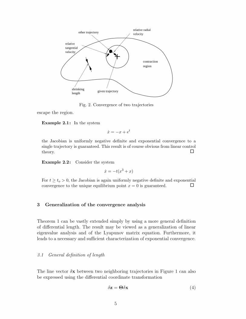
Consider now a ball of constant radius centered about a given trajectory, suchthat given this trajectory the ball remains within a contraction region at alltimes (i.e., ∀t ≥ 0). Because any length within the ball decreases exponentially,any trajectory starting in the ball remains in the ball (since by definition thecenter of the ball is a particular system trajectory) and converges exponentiallyto the given trajectory (Figure 2). Thus, as in stable linear time-invariant (LTI)systems, the initial conditions are exponentially “forgotten.” This leads to thefollowing theorem:

Theorem 1 Given the system equations x = f(x, t), any trajectory, whichstarts in a ball of constant radius centered about a given trajectory and con-tained at all times in a contraction region, remains in that ball and convergesexponentially to this trajectory.

Furthermore, global exponential convergence to the given trajectory is guaran-teed if the whole state space is a contraction region.

This sufficient exponential convergence result may be viewed as a strength-ened version of Krasovskii’s classical theorem on global asymptotic conver-gence (Krasovskii, 1959, page 92; Hahn, 1967, page 270), an analogy we shallgeneralize further in the next section. Note that its proof is very straight-forward, even in the non-autonomous case, and even in the non-global case,where it guarantees explicit regions of convergence. Also, note that the ball inthe above theorem may not be replaced by an arbitrary convex region − whileradial distances would still decrease, tangential velocities could let trajectories

4

relativetangentialvelocity

relative radialvelocity

contraction

region

lengthshrinking

other trajectory

given trajectory

Fig. 2. Convergence of two trajectories

escape the region.

Example 2.1: In the system

x = −x + et

the Jacobian is uniformly negative definite and exponential convergence to asingle trajectory is guaranteed. This result is of course obvious from linear controltheory. 2

Example 2.2: Consider the system

x = −t(x3 + x)

For t ≥ to > 0, the Jacobian is again uniformly negative definite and exponentialconvergence to the unique equilibrium point x = 0 is guaranteed. 2

3 Generalization of the convergence analysis

Theorem 1 can be vastly extended simply by using a more general definitionof differential length. The result may be viewed as a generalization of lineareigenvalue analysis and of the Lyapunov matrix equation. Furthermore, itleads to a necessary and sufficient characterization of exponential convergence.

3.1 General definition of length

The line vector δx between two neighboring trajectories in Figure 1 can alsobe expressed using the differential coordinate transformation

δz = Θδx (4)

5

where Θ(x, t) is a square matrix. This leads to a generalization of our earlierdefinition of squared length

δzT δz = δxTM δx (5)

where M(x, t) = ΘTΘ represents a symmetric and continuously differentiablemetric − formally, equation (5) defines a Riemann space (Lovelock and Rund,1989, page 243). Since (4) is in general not integrable, we cannot expect tofind explicit new coordinates z(x, t), but δz and δzT δz can always be defined,which is all we need. We shall assume M to be uniformly positive definite, sothat exponential convergence of δz to 0 also implies exponential convergenceof δx to 0.

Distance between two points P1 and P2 with respect to the metric M is definedas the shortest path length (i.e., the smallest path integral

∫ P2

P1‖δz‖ ) between

these two points. Accordingly, a ball of center c and radius R is defined as theset of all points whose distance to c with respect to M is strictly less than R.

The two equivalent definitions of length in (5) lead to two formulations ofthe rate of change of length: using local coordinates δz leads to a generaliza-tion of linear eigenvalue analysis (section 3.2), while using the original systemcoordinates x leads to a generalized Lyapunov equation (section 3.3).

3.2 Generalized eigenvalue analysis

Using (4), the time-derivative of δz = Θδx can be computed as

d

dtδz = Θδx + Θδx =

(

Θ + Θ∂f

∂x

)

Θ−1δz = F δz (6)

Formally, the generalized Jacobian

F =

(

Θ + Θ∂f

∂x

)

Θ−1 (7)

represents the covariant derivative of f in δz coordinates (Lovelock and Rund,1989, page 76). The rate of change of squared length can be written

d

dt(δzT δz) = 2 δzT d

dtδz = 2 δzT F δz

Similarly to the reasoning in Theorem 1, exponential convergence of δz (andthus of δx) to 0 can be determined in regions with uniformly negative definite

6

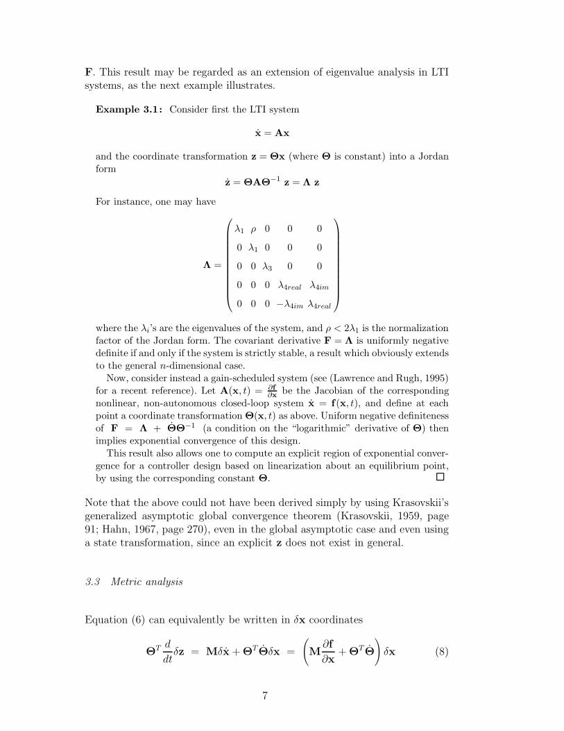
F. This result may be regarded as an extension of eigenvalue analysis in LTIsystems, as the next example illustrates.

Example 3.1: Consider first the LTI system

x = Ax

and the coordinate transformation z = Θx (where Θ is constant) into a Jordanform

z = ΘAΘ−1 z = Λ z

For instance, one may have

Λ =

λ1 ρ 0 0 0

0 λ1 0 0 0

0 0 λ3 0 0

0 0 0 λ4real λ4im

0 0 0 −λ4im λ4real

where the λi’s are the eigenvalues of the system, and ρ < 2λ1 is the normalizationfactor of the Jordan form. The covariant derivative F = Λ is uniformly negativedefinite if and only if the system is strictly stable, a result which obviously extendsto the general n-dimensional case.

Now, consider instead a gain-scheduled system (see (Lawrence and Rugh, 1995)for a recent reference). Let A(x, t) = ∂f

∂xbe the Jacobian of the corresponding

nonlinear, non-autonomous closed-loop system x = f(x, t), and define at eachpoint a coordinate transformation Θ(x, t) as above. Uniform negative definitenessof F = Λ + ΘΘ−1 (a condition on the “logarithmic” derivative of Θ) thenimplies exponential convergence of this design.

This result also allows one to compute an explicit region of exponential conver-gence for a controller design based on linearization about an equilibrium point,by using the corresponding constant Θ. 2

Note that the above could not have been derived simply by using Krasovskii’sgeneralized asymptotic global convergence theorem (Krasovskii, 1959, page91; Hahn, 1967, page 270), even in the global asymptotic case and even usinga state transformation, since an explicit z does not exist in general.

3.3 Metric analysis

Equation (6) can equivalently be written in δx coordinates

ΘT d

dtδz = Mδx + ΘT Θδx =

(

M∂f

∂x+ ΘT Θ

)

δx (8)

7

using the covariant velocity differential Mδx + ΘT Θδx (Lovelock and Rund,1989). The rate of change of length is

d

dt

(

δxTM δx)

= δxT

(

∂f

∂x

T

M + M + M∂f

∂x

)

δx (9)

so that exponential convergence to a single trajectory can be concluded in

regions of ( ∂f∂x

TM + M ∂f

∂x+ M ) ≤ −βMM (where βM is a strictly positive

constant). It is immediate to verify that these are of course exactly the re-gions of uniformly negative definite F in (7). If we restrict the metric M tobe constant, this exponential convergence result represents a generalizationand strengthening of Krasovskii’s generalized asymptotic global convergencetheorem. It may also be regarded as an extension of the Lyapunov matrixequation in LTI systems.

3.4 Generalized contraction analysis

The above leads to the following generalized definition, superseding Definition1 (which corresponds to Θ = I and M = I).

Definition 2 Given the system equations x = f(x, t), a region of the statespace is called a contraction region with respect to a uniformly positive definitemetric M(x, t) = ΘT Θ, if equivalently F in (7) is uniformly negative definite

or ∂f∂x

TM + M ∂f

∂x+ M ≤ −βMM (with constant βM > 0) in that region.

As earlier, regions where F or equivalently ∂f∂x

TM + M ∂f

∂x+ M are negative

semi-definite (skew-symmetric) are called semi-contracting (indifferent). Thegeneralized convergence result can be stated as:

Theorem 2 Given the system equations x = f(x, t), any trajectory, whichstarts in a ball of constant radius with respect to the metric M(x,t), centeredat a given trajectory and contained at all times in a contraction region withrespect to M(x,t), remains in that ball and converges exponentially to thistrajectory.

Furthermore global exponential convergence to the given trajectory is guaran-teed if the whole state space is a contraction region with respect to the metricM(x,t).

In the remainder of this paper we always assume this generalized form whenwe discuss contraction behavior.

8

3.5 A converse theorem

Conversely, consider now an exponentially convergent system, which impliesthat ∃β > 0, ∃k ≥ 1, such that along any system trajectory x(t) and ∀t ≥ 0,

δxT δx ≤ k δxTo δxo e−βt (10)

Defining a metric M(x(t), t) by the ordinary differential equation (Lyapunovequation)

M = −βM− M∂f

∂x−

∂f

∂x

T

M M(t = 0) = kI (11)

and using (9), we can write (10) as

δxT δx ≤ δxT M δx = k δxTo δxo e−βt (12)

Since this holds for any δx, the above shows that M is uniformly positivedefinite, M ≥ I. Thus, any exponentially convergent system is contractingwith respect to a suitable metric.

Note from the linearity of (11) that M is always bounded for bounded t.Furthermore, while M may become unbounded as t → +∞, this does notcreate a technical difficulty, since the boundedness of δxT Mδx (from (12))still implies that δx tends to zero exponentially and also indicates that themetric could be renormalized by a further coordinate transformation.

Thus, Theorem 2 actually corresponds to a necessary and sufficient condi-tion for exponential convergence of a system. In this sense it generalizes andsimplifies a number of previous results in dynamic systems theory.

For instance, note that chaos theory (Guckenheimer and Holmes, 1983; Stro-gatz, 1994) leads at best to sufficient stability results. Lyapunov exponents,which are computed as numerical integrals of the eigenvalues of the symmetricpart of the Jacobian ∂f

∂x, depend on the chosen coordinates x and hence do

not represent intrinsic properties.

3.6 A Note On Krasovskii’s Theorem

It should be clear to the reader familiar with the many versions of Krasovskii’stheorem that by now we have ventured quite far from this classical result.Indeed, Krasovskii’s theorem provides a sufficient, asymptotic convergence

9

result, corresponding to a constant metric M. Also, it does not exploit thepossibility of a pure differential coordinate change as in (4). It is also interest-ing to notice that the type of proof used here is very significantly simpler thanthat used, say, for the global non-autonomous version of Krasovskii’s theorem.This in turn allows many further extensions, as the next sections demonstrate.

3.7 Linear properties of generalized contraction analysis

Introductions to nonlinear control generally start with the warning that thebehavior of general nonlinear non-autonomous systems is fundamentally dif-ferent from that of linear systems. While this is unquestionably the case,contraction analysis extends a number of desirable properties of linear systemanalysis to general nonlinear non-autonomous systems.

(i) Solutions in δz(t) can be superimposed, since ddt

δz = F(x, t)δz around aspecific trajectory x(t) represents a linear time-varying (LTV) system inlocal δz coordinates. Note that the system needs not be contracting forthis result to hold.

(ii) Using this point of view, Theorem 2 can also be applied to other norms,such as ‖δz‖∞ = maxi |δzi| and ‖δz‖1 =

∑

i |δzi|, with associated ballsdefined accordingly. Using the same reasoning as in standard matrix mea-sure results (Vidyasagar, 1992, page 71), the corresponding convergenceresults are

d

dt‖δz‖∞ ≤ max

i(Fii+

∑

j 6=i

|Fij|) ‖δz‖∞d

dt‖δz‖1 ≤ max

j(Fjj+

∑

i6=j

|Fij|) ‖δz‖1

(iii) Global contraction precludes finite escape, under the very mild assump-tion

∃ x∗ , ∃ c ≥ 0, ∀t ≥ 0 , ‖ Θf(x∗, t) ‖ ≤ c

Indeed, no trajectory can diverge faster from x∗ than bounded ‖ Θf(x∗, t) ‖and thus cannot become unbounded in finite time. The result can be ex-tended to the case where x∗ may itself depend on time, as long as itremains in an a priori bounded region.

(iv) A convex contraction region contains at most one equilibrium point, sinceany length between two trajectories is shrinking exponentially in thatregion.

(v) This further implies that, in a globally contracting autonomous system,all trajectories converge exponentially to a unique equilibrium point. In-deed, using V (x) = f(x)T

M(x, t) f(x) as a Lyapunov-like function (anextension of the standard proof of Krasovskii’s Theorem for autonomous

10

systems) yields

V = f(x)T

(

M + M∂f

∂x+

∂f

∂x

T

M

)

f(x) ≤ −βMV

which shows that x = f(x) tends to 0 exponentially, and thus that x

tends towards a finite equilibrium point.(vi) The output of any time-invariant contracting system driven by a periodic

input tends exponentially to a periodic signal with the same period.Indeed, consider a time-invariant nonlinear system driven by a periodic

input ω(t) of period T > 0,

x = f(x, ω(t)) (13)

Let xo(t) be the system trajectory corresponding to the initial conditionxo(0) = xI , and let xT (t) be the system trajectory corresponding to thesystem being initialized instead at xT (T ) = xI . Since f is time-invariantand ω(t) has period T , xT (t) is simply as shifted version of xo(t),

∀t ≥ T, xT (t) = xo(t − T ) (14)

Furthermore, if we now assume that the dynamics (13) is contracting,then initial conditions are exponentially forgotten, and thus xT (t) tendsto xo(t) exponentially. Therefore, from (14), xo(t − T ) tends towardsxo(t) exponentially. By recursion, this implies that ∀t, 0 ≤ t < T , thesequence xo(t + nT ) is a Cauchy sequence, and therefore the limitingfunction limn→+∞ xo(t + nT ) exists, which completes the proof.

(vii) Consider the distance R =∫ P2

P1‖δz‖ between two trajectories P1 and P2 ,

contained at all times in a contraction region characterized by maximaleigenvalues λmax(x, t) ≤ −β < 0 of F. The relative velocity betweenthese trajectories verifies

R + |λmax| R ≤ 0

Assume now, instead, that P1 represents a desired system trajectory andP2 the actual system trajectory in a disturbed flow field x = f(x, t) +d(x, t). Then

R + |λmax| R ≤ ‖Θd‖ (15)

For bounded disturbance ‖Θd‖ any trajectory remains in a boundary ballof (15) around the desired trajectory. Since initial conditions R(t = 0) areexponentially forgotten, we can also state that any trajectory convergesexponentially to a ball of radius R in (15) with arbitrary initial conditionR(t = 0).

(viii) The above can be used to describe a contracting dynamics at multipleresolutions using multiscale approximation of the dynamics with bounded

11

basis functions, as e.g. in wavelet analysis. The radius R with respect tothe metric M of the boundary ball to which all trajectories convergeexponentially becomes smaller as resolution is increased, making precisethe usual “coarse grain” to “fine grain” terminology.

3.8 Combinations of contracting systems

Combinations of contracting systems satisfy simple closure properties, a subsetof which are reminiscent of the passivity formalism (Popov, 1973).

3.8.1 Parallel combination

Consider two systems of the same dimension

x1 = f1(x1, t)

x2 = f2(x2, t)

with virtual dynamics

δz1 =F1 δz

δz2 =F2 δz

and connect them in a parallel combination. If both systems are contractingin the the same metric, so is any uniformly positive superposition

α1(t) δz1 + α2(t) δz2 where ∃ α > 0, ∀t ≥ 0, αi(t) ≥ α (16)

Example 3.2: In the biological motor control community, there has been con-siderable interest recently in analyzing feedback controllers for biological motorsystems as combinations of simpler elements, or motion primitives. For instance(Bizzi, et al., 1993; Mussa-Ivaldi, et al., 1994) have experimentally studied the hy-pothesis that stimulating a small number of areas in a frog’s spinal cord generatescorresponding force fields at the frog’s ankle, and furthermore that these forcefields simply add when different areas are stimulated at the same time. Inter-preting each of these force fields as a contracting flow in joint-space is consistentwith experimental data, and likely candidates for the αi(t) in (16) would thenbe sigmoids and pulses − so-called “tonic” and “phasic” signals (Mussa-Ivaldi,1997; Berthoz, 1993). A simplified architecture may thus consist of weighted con-tracting fields generated at the spinal chord level through high-bandwidth few-synapse feedback connections, combined with the natural viscoelastic propertiesof the muscles, and added open-loop terms generated by the brain, with sometime advance because of the significant nerve transmission delays. 2

12

3.8.2 Feedback Combination

Similarly, connect instead two systems of possibly different dimensions

x1 = f1(x1,x2, t)

x2 = f2(x1,x2, t)

in the feedback combination

d

dt

δz1

δz2

=

F1 G

− GT F2

δz1

δz2

The augmented system is contracting if and only if the separated plants arecontracting.

3.8.3 Hierarchical Combination

Consider a smooth virtual dynamics of the form

d

dt

δz1

δz2

=

F11 0

F21 F22

δz1

δz2

and assume that F21 is bounded. The first equation does not depend on thesecond, so that exponential convergence of δz1 to zero can be concluded foruniformly negative definite F11. In turn, F21δz1 represents an exponentiallydecaying disturbance in the second equation. Similarly to remark (vii) in sec-tion 3.7, a uniformly negative definite F22 implies exponential convergence ofδz2 to an exponentially decaying ball. Thus, the whole system globally expo-nentially converges to a single trajectory.

By recursion, the result can be extended to systems similarly partitioned inmore than two equations. It may be viewed as providing a general commonframework for sliding control concepts, singular perturbations, and triangularsystems, where such hierarchical analysis can be found (see also (Simon, 1981)in a broader context).

Consider again the system above, but now with disturbance Θ1d1 added tothe δz1 dynamics and Θ2d2 added to the δz2 dynamics. This means that therelative velocities between a desired trajectory P1 and a system trajectory P2

verify

13

d

dt

P2∫

P1

‖δz1‖ + |λmax1|

P2∫

P1

‖δz1‖ ≤ ‖Θ1d1‖

d

dt

P2∫

P1

‖δz2‖ + |λmax2|

P2∫

P1

‖δz2‖ ≤ ‖Θ2d2‖ +

P2∫

P1

F21δz1

Bounded disturbances Θ1d1 and Θ1d2 thus imply exponential convergence toa ball around the desired trajectory.

Example 3.3: Chain reactions are classical examples of hierarchical dynamics.Consider for instance a standard polymerization process in an open stirred tank(adapted from (Adebekun and Schork, 1989)), of the form

I =q

V(If − I) − kd e−

EdRT I

M =q

V(Mf − M) − 2kp e−

Ep

RT M2I

P =q

V(Pf − P ) + kp e−

Ep

RT M2I

T =q

V(Tf − T ) +

(

−∆H

ρcp

)

kpM2I −

hAc

V ρcp(T − Tc)

with I, M , and P being the initiator, monomer, and polymer concentrations,T the temperature, Tc the coolant temperature, q(t) > 0 the feed flow rate, V

the reactor volume, kp and kd positive reaction constants, and the subscript f

corresponding to feed values. Consider now a reduced-order identity observer onI, M , and P whose reaction rates simply reproduce the model using the measuredtemperature T (t),

˙I =

q

V

(

If − I)

− kd e−EdRT I

˙M =

q

V

(

Mf − M)

− 2kp e−Ep

RT M2I

˙P =

q

V

(

Pf − P)

+ kp e−Ep

RT M2I

Since this observer represents a hierarchical system, the uniform negative defi-

niteness of ∂˙I

∂I, ∂

˙M

∂M, and ∂

˙P

∂Pimplies that it converges exponentially. 2

Example 3.4: Contraction analysis may be used as a more precise alternativeto zero-dynamics analysis (Isidori, 1995). Consider an n-dimensional system x =f(x,u, t) with measurement y = h(x, t). Assume that repeated differentiation ofthe measurement leads to y(p) = g(x,u, t) with p ≤ n, where we can choose acontrol input that leads to a contracting linear design in y, ...,y(p).

Contracting behavior of the (n−p)-dimensional remaining states z and thus ofthe whole system can then be concluded according to section 3.8.3 for uniformlynegative definite ∂z

∂z. 2

14

Note that the properties above can be arbitrarily combined.

Example 3.5: Using the hierarchical property, the open-loop signal generatedby the brain in the biological motor control model of Example 3.2 may itself bethe output of a contracting dynamics. So can be the αi(t), since the correspondingprimitives are bounded. In principle, the contraction property would also enablethis term to be learned (see also (Droulez, et al., 1983; Flash, 1995; Mussa-Ivaldi,1997)) by making the system’s behavior consistent in the presence of disturbancesor variations in initial conditions.

In this context, the remark (vi) on periodic inputs in section 3.7 may alsobe relevant to the periodic phenomena pervasive in physiology. These include,for instance, the rhythmic motor behaviors used in locomotion and driven bycentral pattern generators, as in walking, swimming, or flying (Kandel, et al.,1991; Dowling, 1992), as well as automatic mechanisms such as breathing andheart cycles. 2

3.9 Additional Remarks

In addition to the simple properties above, we can make a few more technicalremarks and extensions on Theorem 2.

• Theorem 2 may be viewed as a more precise version of Gauss theorem influid mechanics

d

dtδV = div(

d

dtδz) δV

which shows that any volume element δV shrinks exponentially to zero foruniformly negative definite div( d

dtδz), implying convergence to an (n − 1)-

dimensional manifold rather than to a single trajectory. Indeed, div( ddt

δz)is just the trace of F.

• Theorem 2 still holds if the radius R of the ball is time-varying, as longas trajectories starting in the ball can be guaranteed to remain in the ball.Given (7) and F ≤ −β I < 0 this is the case if ∀t ≥ 0, R + β ≥ 0 .

• Assume that the metric M is only positive semi-definite, with some principaldirections pi corresponding to uniformly positive definite eigenvalues of M.Uniformly negative definiteness of F then implies exponential convergenceto zero of the components of δx on the linear subspace spanned by the pi .

• Assume that F is not uniformly negative definite, but rather that ∃ κ >

0, ∃ to > 0, ∀t ≥ to,F ≤ −1tκI. Since

∫ tto

1τκ dτ tends to +∞ as t → +∞, any

infinitesimal length converges asymptotically (although not necessarily ex-ponentially) to zero, and thus asymptotic convergence to a single trajectorycan be concluded.

• Any regular Θ(x), defined in a compact set in x, yields a uniformly positivedefinite metric M = ΘT Θ in this compact set.

• Since trajectories can rotate or oscillate around each other, overshoots mayoccur in the elongated principal directions of the metric M(x, t).

15

• In the case that an explicit z(x, t) exists, we can alternatively compute thevirtual velocity from z = ∂z

∂xf + ∂z

∂t, since then

δz = δ

(

∂z

∂xf +

∂z

∂t

)

=∂2z

∂x2δx f +

∂z

∂x

∂f

∂xδx +

∂z2

∂t∂xδx =

d

dtδz

• Contraction analysis can also be applied to differential coordinates δz whosedimension is not the same as that of x. Of course, lower-dimensional coor-dinates can only lead to positive semi-definite metrics M.

• Contraction regions of an arbitrary autonomous dynamic system x = f(x)may be computed by solving (in general numerically) the partial differentialequation in space

∂Θ

∂xf + Θ

∂f

∂x= −Θ

with appropriate boundary conditions, which imposes F = − I . Considerfor instance the plant

x = − sin x

and set Fθ = − dθdx

sin x − θ cos x = −θ . Integrating with θ(0) = 1 (to be

consistent with linearization) leads to θ =tan x

2

sinx. The metric is singular at

x = π +2nπ with n ∈ Z, so that contraction regions are ]2nπ−π, 2nπ +π[.• Theorem 2 can also be used to show exponential divergence of two neighbor-

ing trajectories. Indeed, if the minimal eigenvalue λmin(x, t) of the symmet-ric part of the F is strictly positive, then equation (3) implies exponentialdivergence of two neighboring trajectories. This may be used to imposeconstraints on the flow (or, by state-augmentation, the input).

4 Applications of Contraction Analysis

This section illustrates the discussion with some immediate applications ofcontraction analysis to specific control and estimation problems.

4.1 PD observers

Observer design using contraction analysis can be simplified by prior coor-dinate transformations similar to those used in linear reduced-order observerdesign (Luenberger, 1979). Consider the system

x= f(x, t)

y =h(x, t)

16

where x is the state vector and y the measurement vector. Define a stateobserver with

˙x= f(x, t) − KP (y − y) −KDˆy (17)

x= x + KDy

where y = h(x, t) and ˆy = ∂y

∂xf(x, t) + ∂h

∂t. By differentiation, this leads to the

observer dynamics

˙x = f(x, t) − KP (y − y) − KD

(

ˆy − y)

Thus the dynamics of x contains y, although the actual computation is doneusing equation (17) and hence y is not explicitly used.

Example 4.1: Consider a simple model of underwater vehicle motion, includingthruster dynamics

q1

q2

=

τ(t) − 3q1 |q1|

−10 q2 |q2| + q1 |q1|

where y1 = q1 is the measured propeller angle, y2 = q2 the measured vehicleposition, q1 |q1| the propeller thrust, q2 |q2| the vehicle drag, and τ(t) the torqueinput to the propeller (Figure 3). The system dynamics is heavily damped forlarge |q1| and |q2|. However, this natural damping is ineffective at low velocities.Letting ω = q1 , v = q2 , this suggests using a coordinate error feedback in thereduced-order observer

q

1

2

τq , (t)

Fig. 3. Underwater vehicle

˙ω

˙v

=

τ(t) − 3ω |ω| − kd1ω

−10 v |v| + ω |ω| − kd2v

ω

v

=

ω + kd1q1

v + kd2q2

where kd1 and kd2 are strictly positive constants. This leads to the hierarchicaldynamics

˙ω

˙v

=

τ(t) − 3ω |ω| − kd1(ω − ω)

−10 v |v| + ω |ω| − kd2(v − v)

17

The uniform negative definiteness of ∂ ˙ω∂ω

= (−3 |ω|−kd1) and ∂ ˙v∂v

= (−10 |v|−kd2)(which is implied by our choice of strictly positive constants kdi) guarantees expo-nential convergence to the actual system trajectory, which is indeed a particularsolution.

System responses to the input

τ =

5 for 0 ≤ t < 1

−10 for 1 ≤ t < 2

with initial conditions ω(0) = 0, ω(0) = 4 or −4, v(0) = 5, v(0) = −10 or 20 andfeedback gains kd1 = kd2 = 5 are illustrated in Figure 4. The solid line representsthe actual plant and the dashed lines the observer estimates. 2

0 0.5 1 1.5 2−4

−3

−2

−1

0

1

2

3

4

PR

OP

ELL

ER

VE

LOC

ITY

TIME0 0.5 1 1.5 2

−10

−5

0

5

10

15

20

VE

HIC

LE V

ELO

CIT

Y

TIME

Fig. 4. Underwater vehicle observer

4.2 Constrained Systems

Many physical systems, such as mechanical systems with kinematic constraintsor chemical systems in partial equilibrium, are described by an original n-dimensional dynamics of the form

z = f(z, t)

constrained to an explicit m-dimensional submanifold (m ≤ n)

z = z(x, t)

The constrained dynamic equations are then of the form

z = f(z, t) + n

where n represents a superimposed flow normal to the manifold, ∂z∂x

Tn = 0

− the components of n are Lagrange parameters. In a mechanical system, z

represents unconstrained positions and velocities, x generalized coordinates

18

and associated velocities, and n constraint forces. Multiplying from the left

with ∂z∂x

Tresults in

∂z

∂x

T

z =∂z

∂x

T(

∂z

∂xx +

∂z

∂t

)

=∂z

∂x

T

f(z) (18)

so that a uniformly positive definite metric M = ∂z∂x

T ∂z∂x

allows one to compute,

with x = M−1 ∂z∂x

T(

f(z, t) − ∂z∂t

)

n = z − f =∂z

∂t+

∂z

∂xM−1 ∂z

∂x

T(

f −∂z

∂t

)

− f

The variation of (18) is

∂z

∂x

T

δz = −∂2z

∂x2

T

n δx +∂z

∂x

T ∂f

∂zδz

so that

1

2

d

dt(δxTMδx) = δxT ∂z

∂x

T ∂f

∂z

∂z

∂xδx − δxT ∂2z

∂x2n δx (19)

Consider now a specific trajectory zd(t) of the unconstrained flow field whichnaturally remains on the manifold z(x, t). Then the normal flow n around thistrajectory vanishes, so that locally the contraction behavior is determined bythe projection of the original Jacobian

Jd =∂z

∂x

T ∂f

∂z

∂z

∂x(20)

Contraction of the original unconstrained flow thus implies local contractionof the constrained flow, and the contraction region around the trajectory canbe computed with (19).

This result can be used to study the contraction behavior of mechanical sys-tems with linear external forces, such as PD terms or gravity − Newton’s lawin the original unconstrained state space is then linear, and z = z(x, t) arekinematic constraints. Exponential convergence around one trajectory z(t) atwhich the constraint forces vanish can then be concluded in the region wherethe projection (20) of the original constant Jacobian ∂f

∂zis uniformly negative

definite. Exponential convergence of a controller or observer (see also (Marinoand Tomei, 1995; Berghuis and Nijmeyer, 1993)) can thus be achieved bystabilizing the unconstrained dynamics with a PD part, and adding an open-loop control input to guarantee that a desired trajectory consistent with thekinematic constraints is indeed contained in the unconstrained flow field.

19

4.3 Linear Time-Varying Systems

As another illustration, this section shows that contraction analysis can beused systematically to control and observe linear time-varying (LTV) systems.

4.3.1 LTV controllers

Consider a general smooth linear time-varying system

x = A(t)x + b(t)u

with control input u = K(t)x+ud(t). We focus on choosing the gain K(t) so asto achieve contraction behavior; whereas the open-loop term ud(t) then guar-antees that the desired trajectory, if feasible, is indeed contained in the flowfield (this guarantee and a similar computation is required of any controllerdesign).

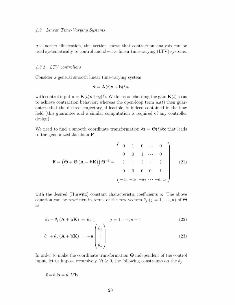
We need to find a smooth coordinate transformation δz = Θ(t)δx that leadsto the generalized Jacobian F

F =(

Θ + Θ (A + bK))

Θ−1 =

0 1 0 · · · 0

0 0 1 · · · 0...

......

. . ....

0 0 0 0 1

−ao −a1 −a2 · · · −an−1

(21)

with the desired (Hurwitz) constant characteristic coefficients ai. The aboveequation can be rewritten in terms of the row vectors θj (j = 1, · · · , n) of Θ

as

θj + θj (A + bK) = θj+1 j = 1, · · · , n − 1 (22)

θn + θn (A + bK) = −a

θ1

...

θn

(23)

In order to make the coordinate transformation Θ independent of the controlinput, let us impose recursively, ∀t ≥ 0, the following constraints on the θj

0= θ1b = θ1Lob

20

0= θ2b =(

θ1 + θ1A)

b−d

dt(θ1b) = θ1L

1b

0= θ3b =(

θ2 + θ2A)

b−d

dt(θ2b) = θ2L

1b (24)

=(

θ1 + θ1A)

L1b−d

dt

(

θ1L1b)

= θ1L2b

...

D = θnb = θ1Ln−1b

where the Ljb are generalized Lie derivatives (Lovelock and Rund, 1989)

L0b=b

Lj+1b=A Ljb−d

dtLjb j = 0, ..., n − 1 (25)

Choosing D = det |Lob ... Ln−1b| the above can always be solved algebraicallyfor a smooth θ1, and from (22) the remaining smooth θj can then be computedalgebraically using the recursion

θj+1 = θj + θjA j = 1, · · · , n − 1

This leads to a smooth bounded metric, and the feedback gain K(t) can thenbe computed from (23)

D K(t) = −a

θ1

...

θn

− θn − θnA

Exponential convergence of δx is then guaranteed for uniformly positive def-inite metric M = ΘTΘ. The uniform positive definiteness of M hence repre-sents a sufficient “contractibility” condition.

Note that the terms θi and ddt

Lib distinguish this derivation from the usualpole-placement in an LTI system, as well as from related gain-scheduling tech-niques (Wu, Packard, and Bals, 1995; Mracek, Cloutier, and D’Souza, 1996).The method guarantees global exponential convergence, and can be extendedstraightforwardly to multi-input systems.

4.3.2 LTV observers

Similarly, consider again the plant above, but assume that only the measure-ment y = C(t)x + d(t) is available. Define the observer

˙x = A(t)x + E(t) (y − c(t)x + d(t)) + b(t)u

21

Since by definition the actual state is contained in the flow field, no “open-loop” term is needed, but we need to find a smooth coordinate transformationδx = Σ(t)δz that leads to the generalized Jacobian F

F = Σ−1(

−Σ + (A− Ec)Σ)

=

0 0 · · · 0 −ao

1 0 · · · 0 −a1

0 1 · · · 0 −a2

......

. . . 0...

0 0 · · · 1 −an−1

(26)

with the desired (Hurwitz) constant characteristic coefficients ai. The aboveequation can be rewritten in term of the column vectors σj of Σ as

−σj + (A− Ec)σj = σj+1 j = 1, · · · , n − 1 (27)

−σn + (A − Ec)σn =−(

σ1 · · · σn

)

a (28)

Proceeding as before by imposing the constraints

Ljc σ1 = 0 j = 0, ..., n − 2

Ln−1c σ1 = det∣

∣

∣Loc ... Ln−1c∣

∣

∣

where the Ljc are now defined as

Loc= c

Lj+1c=Ljc A +d

dtLjc j = 0, ..., n − 1 (29)

allows one to solve algebraically for a smooth σ1, and then compute the re-maining smooth σj recursively

σj+1 = −σj + Aσj j = 1, · · · , n − 1

leading to a uniformly positive definite metric. The feedback gain E(t) canthen be computed from (28)

ED =(

σ1 · · · σn

)

a − σn + Aσn

Exponential convergence of δx to zero and thus of x to x is then guaranteedfor a bounded metric M = Σ−TΣ . The boundedness of M hence representsa sufficient observability condition.

22

Again, the terms σi and ddt

Lic distinguish this derivation from pole-placementin LTI systems, or from extended Kalman filter-like designs (Bar-Shalom andFortmann, 1988). The method guarantees global exponential convergence, andcan be extended straightforwardly to multi-output systems.

4.3.3 Separation principle

These LTV designs satisfy a separation principle. Indeed, let us combine theabove controller and observer (perhaps with different coefficient vectors a)

u = K(t)x + ud(t)

Subtracting the plant dynamics from the observer dynamics leads with x =x − x to

˙x=(A(t) − E(t)C(t)) x

so that the Jacobian of the error-dynamics of the observer is unchanged. Sincethe observer error-dynamics and the controller dynamics represent a hierar-chical system, they can be designed separately as long as the control gain K(t)is bounded.

Remark (vii) in section 3.7 can be used to assess the robustness of these designsto additive modeling uncertainties.

4.3.4 Nonlinear controllers and observers

Consider now the nonlinear system

δx =∂f

∂xδx +

∂f

∂uδu δy =

∂h

∂xδx

Let

A(t) =∂f

∂x(xd(t), t) B(t) =

∂f

∂u(xd(t), t) c(t) =

∂h

∂x(xd(t), t)

where xd(t) is the desired trajectory. Applying the controller and observer de-signs above to the LTV system defined by A(t), b(t), and c(t) then guaranteescontraction behavior in regions of uniformly negative definite

Fcontrol =

(

Θ(xd(t), t) + Θ(xd(t), t)

(

∂f

∂x(x, t) +

∂f

∂u(x, t)K(xd(t), t)

))

Θ(xd(t), t)−1

23

and

Fobs = Σ(xd(t)−1

(

−Σ(xd(t), t) +

(

∂f

∂x(x, t) − E(xd(t), t)

∂h

∂x(x, t)

)

Σ(xd(t), t)

)

similarly to Example 3.1. Thus exponential convergence is guaranteed explic-itly in a given finite region around the desired trajectory.

5 The discrete-time case

Theorem 1 can be extended to discrete-time systems

xi+1 = fi(xi, i)

The associated virtual dynamics is

δxi+1 =∂fi

∂xi

δxi

so that the virtual length dynamics is

δxTi+1δxi+1 = δxT

i

∂fi

∂xi

T ∂fi

∂xi

δxi

Thus, exponential convergence to a single trajectory is guaranteed for

∂fi

∂xi

T ∂fi

∂xi

− I ≤ −βI < 0

This may be viewed as extending to non-autonomous systems the standarditerated map results based on the contraction mapping theorem. The conver-gence condition is equivalent to requiring that the largest singular value ofthe Jacobian ∂fi

∂xiremain smaller than 1 uniformly. A discrete-time version of

Theorem 2 can be derived similarly, using the generalized virtual displacement

δzi = Θi(xi, i)δxi

leading to

δzTi+1δzi+1 = δxT

i

∂fi

∂xi

T

ΘTi+1Θi+1

∂fi

∂xi

δxi = δzTi FT

i Fiδzi

with the discrete generalized Jacobian

Fi = Θi+1∂fi

∂xi

Θ−1i (30)

24

Note the similarity and difference with the Jacobian of an LTI system. Theabove leads to the following generalized definition for discrete-time systems.

Definition 3 Given the discrete-time system equations xi+1 = fi(xi, i), a re-gion of the state space is called a contraction region with respect to a uniformlypositive definite metric Mi(xi, i) = ΘT

i Θi, if in that region

∃β > 0, FTi Fi − I ≤ −βI < 0

where Fi = Θi+1∂fi∂xi

Θ−1i .

Theorem 2 can then be immediately extended as

Theorem 3 Given the system equations xi+1 = fi(xi, i), any trajectory, whichstarts in a ball of constant radius with respect to the metric Mi, centered at agiven trajectory and contained at all times in a generalized contraction region,remains in that ball and converges exponentially to this trajectory.

Furthermore global exponential convergence to the given trajectory is guaran-teed if the whole state space is a contraction region with respect to the metricMi.

Most of our earlier continuous-time results have immediate discrete-time ver-sions, as detailed in (Lohmiller and Slotine, 1997d).

Example 5.1: As in the continuous-time case, consider first the discrete-timeLTI system

xi+1 = Axi

and the coordinate transformation zi = Θxi (where Θ is constant) into a Jordanform

zi+1 = ΘAΘ−1 zi = Λ zi

It is straightforward to show that ΛTΛ − I is uniformly negative definite if andonly if the system is strictly stable.

Now, consider instead a discrete-time gain-scheduled system. Let Ai(xi, i) =∂fi∂xi

be the Jacobian of the corresponding nonlinear, non-autonomous closed-loopsystem xi+1 = fi(xi, i), and define at each point a coordinate transformationΘi as above. Uniform negative definiteness of ΛTΛ− I then implies exponentialconvergence of this design.

This result also allows one to compute an explicit region of exponential conver-gence for a controller design based on linearization about an equilibrium point,by using the corresponding constant Θi. 2

25

6 Concluding remarks

By using a differential approach, convergence analysis and limit behavior arein a sense treated separately. Guaranteeing contraction means that after ex-ponential transients the system’s behavior will be independent of the initialconditions. In an observer context, one then needs only verify that the observerequations contain the actual plant state as a particular solution to automati-cally guarantee convergence to that state. In a control context, once contrac-tion is guaranteed through feedback, specifying the final behavior reduces tothe problem of shaping one particular solution, i.e. specifying an adequateopen-loop control input to be added to the feedback terms, a necessary stepof any control method.

Current research includes systematically guaranteeing global exponential con-vergence for general nonlinear systems, stable adaptation to unknown param-eters, and further applications to mechanical and chemical systems.

Acknowledgments: This paper benefited from discussions with Ch. Bernardand G. Niemeyer, and from reviewers’ comments and suggestions.

REFERENCES

Adebekun, D.K., and Schork, F.J. (1989). Continuous solution polymerizationreactor control. 1. Nonlinear reference control of methyl methacrylate polymeriza-tion, Industrial Engineering and Chemical Research, 28:1308 - 1324.Arnold, V.I. (1978). Mathematical Methods of Classical Mechanics, SpringerVerlag.Bar-Shalom Y., and Fortmann, T. (1988). Tracking and Data Association,Academic Press.Berghuis, H., and Nijmeyer, H. (1993). A passivity-based approach to controller-observer design for robots, I.E.E.E. Transactions on Robotics and Automation, 9(6).Berthoz, A., Ed. (1993). Multisensory Control of Movement, Oxford UniversityPress.Bizzi E., Giszter S.F., Loeb E., Mussa-Ivaldi F.A., Saltiel P (1995). Mod-ular organization of motor behavior in the frogs’s spinal cord. Trends in Neuro-sciences. Review 18:442-446Dowling, J.E. (1992). Neurons and Networks, Belknap.Droulez, J., et al. (1983). Motor Control, 7th International Symposium of theInternational Society of Posturography, Houston, Karger, 1985.Flash, T. (1995). Trajectory Learning and Control Models, I.F.A.C. Man-MachineSystems Symposium, Cambridge, MA.Guckenheimer, J., and Holmes, P. (1983). Nonlinear Oscillations, DynamicalSystems, and Bifurcations of Vector Fields, Springer Verlag.Hahn, W. (1967). Stability of motion, Springer Verlag.Isidori, A. (1995). Nonlinear Control Systems, 3rd Ed., Springer Verlag.Kandel, E.R., Schwartz, J.H., and Jessel, T.M. (1991). Principles of Neural

26

Science, Appleton and Lange.Khalil, H. (1995). Nonlinear Systems, 2nd Ed., Prentice-Hall.Krasovskii, N.N. (1959). Problems of the Theory of Stability of Motion, Mir,Moskow. English translation by Stanford University Press, 1963.Lawrence, D.A., and Rugh, W.J. (1995). Gain-scheduling dynamic linear con-trollers for a nonlinear plant, Automatica, 31(3).Lohmiller, W., and Slotine, J.J.E. (1996a). Metric Observers for Nonlin-ear Systems, I.E.E.E. International Conference on Control Applications, Dearborn,Michigan.Lohmiller, W., and Slotine, J.J.E. (1996b). Applications of Metric Observersfor Nonlinear Systems, I.E.E.E. International Conference on Control Applications,Dearborn, Michigan.Lohmiller, W., and Slotine, J.J.E. (1996c). On Metric Controllers for Nonlin-ear Systems, I.E.E.E. Conference on Decision and Control, Kobe, Japan.Lohmiller, W., and Slotine, J.J.E. (1997a). Practical Observers for Hamilto-nian Systems, I.E.E.E. American Control Conference, Albuquerque, New Mexico.Lohmiller, W., and Slotine, J.J.E. (1997b). Applications of Contraction Anal-ysis, I.E.E.E. Conference on Control Applications, Hartford, Connecticut.Lohmiller, W., and Slotine, J.J.E. (1997c). Applications of Contraction Anal-ysis, I.E.E.E. Conference on Decision and Control, San Diego, California.Lohmiller, W., and Slotine, J.J.E. (1997d). Contraction Analysis: The Discrete-Time Case, MIT-NSL Report 971101, November 1997.Lovelock, D., and Rund, H. (1989). Tensors, differential forms, and variationalprinciples, Dover.Luenberger, D. G. (1979). Introduction to Dynamic Systems, John Wiley &Sons.Mracek, P., Cloutier, J., D’Souza C. (1996 A new Technique for NonlinearEstimation, I.E.E.E. International Conference on Control Applications, Dearborn,Michigan.Marino, R., and Tomei, T. (1995). Nonlinear Control, Prentice-Hall.Mussa-Ivaldi, F.A. (1997). Nonlinear Force Fields: a distributed system of con-trol primitives for representing and learning movements, 1997 IEEE InternationalSymposium on Computational Intelligence in Robotics and Automation, pp. 84-90.Mussa-Ivaldi, F.A., Giszter S.F., Bizzi E. (1994). Linear Superposition ofprimitives in motor control. Proceedings and National Academy of Sciences. 91:7534-7538.Nijmeyer, H., and Van der Schaft, A. (1990). Nonlinear Dynamical ControlSystems, Springer Verlag.Popov, V.M. (1973). Hyperstability of Control Systems, Springer-Verlag.Schwartz, L. (1993). Analyse, Hermann, Paris.Simon, H.A. (1981). The Sciences of the Artificial, 2nd edition, MIT Press.Slotine, J.J.E., and Li, W. (1991). Applied Nonlinear Control, Prentice-Hall.Strogatz, S. (1994). Nonlinear Dynamics and Chaos, Addison Wesley.Vidyasagar, M. (1992). Nonlinear Systems Analysis, 2nd Edition, Prentice-Hall.Wu, F., Packard, A., Bals G. (1995). LPV Control Design for Pitch-Axis Mis-sile Autopilots. I.E.E.E. International Conference on Decision and Control, NewOrleans, Louisiana.

27