ON CIRCUIT COMPLEXITY CLASSES AND ITERATEDMATRIX MULTIPLICATION

BY FENGMING WANG

A dissertation submitted to the

Graduate School—New Brunswick

Rutgers, The State University of New Jersey

in partial fulfillment of the requirements

for the degree of

Doctor of Philosophy

Graduate Program in Computer Science

Written under the direction of

Eric Allender

and approved by

New Brunswick, New Jersey

January, 2012

ABSTRACT OF THE DISSERTATION

On Circuit Complexity Classes and Iterated Matrix Multiplication

by Fengming Wang

Dissertation Director: Eric Allender

In this thesis, we study small, yet important, circuit complexity classes within NC1, such as

ACC0 and TC0. We also investigate the power of a closely related problem called Iterated

Matrix Multiplication and its implications in low levels of algebraic complexity theory. More

concretely,

• We show that extremely modest-sounding lower bounds for certain problems can lead to

non-trivial derandomization results.

– If the word problem over S5 requires constant-depth threshold circuits of size n1+ε

for some ε > 0, then any language accepted by uniform polynomial-size probabilis-

tic threshold circuits can be solved in subexponential time (and more strongly, can

be accepted by a uniform family of deterministic constant-depth threshold circuits

of subexponential size.)

– If there are no constant-depth arithmetic circuits of size n1+ε for the problem of

multiplying a sequence of n 3-by-3 matrices, then for every constant d, black-box

identity testing for depth-d arithmetic circuits with bounded individual degree can

be performed in subexponential time (and even by a uniform family of deterministic

constant-depth AC circuits of subexponential size).

ii

• ACCm circuits are circuits consisting of unbounded fan-in AND, OR and MODm gates

and unary NOT gates, where m is a fixed integer. We show that there exists a language

in non-deterministic exponential time which can not be computed by any non-uniform

family of ACCm circuits of quasi-polynomial size and o(log log n) depth, where m is an

arbitrarily chosen constant.

• We show that there are families of polynomials having small depth-two arithmetic cir-

cuits that cannot be expressed by algebraic branching programs of width two. This clari-

fies the complexity of the problem of computing the product of a sequence of two-by-two

matrices, which arises in several settings.

iii

Acknowledgements

I would like to express my gratitude to everybody who helped me during my life at Rutgers.

First and foremost, I am very grateful to my advisor Eric Allender, for his enlightening

guidance and unselfish support. Throughout these years he has always been willing and man-

aged to spend time with me, answer my questions and even discuss problems in my personal

life. Eric has been very patient to listen to my ideas which were often nonsensical and never

tired of my poor English grammar. He is truly a wonderful friend of mine.

I would like to express my gratitude to my co-advisor Mike Saks for his great discussions

and for organizing Theory Reading Seminars. Mike has always been full of creative ideas,

sharp insights and enthusiastic encouragement. He is a Mathematics genius and an excellent

teacher.

I would like to thank Mario Szegedy and Russell Impagliazzo for volunteering to serve on

my dissertation committee. I would like to thank Vikraman Arvind, Troy Lee, Nikos Leonardos

and Rahul Santhanam for collaborating with me.

Rutgers has a fantastic group of faculty on Theoretical Computer Science and Mathematics.

Over the years, I have benefited a lot from courses taught by Jeff Kahn, Michael Kiessling,

Janos Komlos, Mike Saks, Bill Steiger, Mario Szegedy, Endre Szemeredi, Van Vu and Chuck

Weibel. I would like to thank them for the mind-opening lectures and for allowing me to ask

stupid questions.

My fellow students at Rutgers made my journey as a graduate student much easier. The

lunch discussions with Devendra Desai, Luke Friedman, Mangesh Gupte, Nikos Leonardos,

Rajat Mittal, Peter Richter, Lei Wang and Yixin Xu were filled with fun. Without their compan-

ion, the trips to attend various conferences and workshops would not have been so delightful.

I would like to thank Carol DiFrancesco and other staff at Rutgers for their constant patience

to solve all of administrative problems. Whenever I needed Carol’s favor, she never hesitated

iv

to help me out. To me, Carol is the role model for every Graduate Secretary.

I would like to thank Aduri Pavan, my Master thesis advisor, for his guidance and support

during the initial stage of my research life. I would like to thank Xiaoyang Gu, one of my best

friends, for bringing me into the world of Complexity Theory and for helping me solve many

technical and non-technical problems over the years.

Research conducted in this thesis was supported in part by NSF grants CCF-0830133, CCF-

0832787 and CCF-1064785.

v

Dedication

Dedicated to my parents and my wife Cui, without whose support over the years, this would

never have happened.

vi

Table of Contents

Abstract . . . . . . . . . . . . . . . . . . . . . . . . . . . . . . . . . . . . . . . . . ii

Acknowledgements . . . . . . . . . . . . . . . . . . . . . . . . . . . . . . . . . . . iv

Dedication . . . . . . . . . . . . . . . . . . . . . . . . . . . . . . . . . . . . . . . . vi

1. Introduction . . . . . . . . . . . . . . . . . . . . . . . . . . . . . . . . . . . . . 1

1.1. AC0, AC0(MODp) and ACC0 . . . . . . . . . . . . . . . . . . . . . . . . . . . 2

1.2. TC0 and NC1 . . . . . . . . . . . . . . . . . . . . . . . . . . . . . . . . . . . 6

1.3. On Iterated Matrix Multiplication . . . . . . . . . . . . . . . . . . . . . . . . 9

1.3.1. Identity Testing for Constant-depth Arithmetic Circuits . . . . . . . . . 10

1.3.2. Impossibility Result for IMM2,n . . . . . . . . . . . . . . . . . . . . . 12

2. Uniform Derandomization from Pathetic Lower Bounds . . . . . . . . . . . . . 16

2.1. Background on Derandomization . . . . . . . . . . . . . . . . . . . . . . . . . 16

2.2. Preliminaries . . . . . . . . . . . . . . . . . . . . . . . . . . . . . . . . . . . 18

2.3. The existence of an average-case hard language . . . . . . . . . . . . . . . . . 19

2.3.1. Worst-case to Average-case Reduction for NC1 . . . . . . . . . . . . . 19

2.3.2. Worst-case to Average-case Reduction for L . . . . . . . . . . . . . . . 24

2.3.3. Worst-case to Average-case Reduction for GapL and GapNC1 . . . . . 27

2.4. Uniform derandomization . . . . . . . . . . . . . . . . . . . . . . . . . . . . . 30

2.5. Consequences of pathetic arithmetic circuit lower bounds . . . . . . . . . . . . 33

3. Non-constant-depth Lower Bounds for NEXP against ACC circuits . . . . . . . 40

3.1. Preliminaries . . . . . . . . . . . . . . . . . . . . . . . . . . . . . . . . . . . 40

3.2. Main Proof . . . . . . . . . . . . . . . . . . . . . . . . . . . . . . . . . . . . 41

3.2.1. A Fast Satisfiability Algorithm . . . . . . . . . . . . . . . . . . . . . . 41

vii

3.2.2. Proof of Theorem 3 . . . . . . . . . . . . . . . . . . . . . . . . . . . . 42

3.3. Discussions . . . . . . . . . . . . . . . . . . . . . . . . . . . . . . . . . . . . 45

4. On the Power of IMM2,n . . . . . . . . . . . . . . . . . . . . . . . . . . . . . . 46

4.1. Preliminaries . . . . . . . . . . . . . . . . . . . . . . . . . . . . . . . . . . . 46

4.2. IMM2,n under homogeneous projections . . . . . . . . . . . . . . . . . . . . . 50

4.2.1. Classification of H2×2 ∩ Indg . . . . . . . . . . . . . . . . . . . . . . 50

4.2.2. Structure of µH2×2∩Indg-SLPs and its implications . . . . . . . . . . . 52

4.2.3. Limitation of µH2×2-SLPs . . . . . . . . . . . . . . . . . . . . . . . . 56

4.3. Extensions to simple and regular projections . . . . . . . . . . . . . . . . . . . 62

4.3.1. Impossibility result for simple projections . . . . . . . . . . . . . . . . 62

4.3.2. Impossibility result for regular projections . . . . . . . . . . . . . . . . 65

References . . . . . . . . . . . . . . . . . . . . . . . . . . . . . . . . . . . . . . . . 70

Vita . . . . . . . . . . . . . . . . . . . . . . . . . . . . . . . . . . . . . . . . . . . 79

viii

1

Chapter 1

Introduction

In complexity theory, a computational problem is usually represented by a subset of 0, 1∗,

which is called a language. Within this research area, one of the major goals is to classify

languages according to the amount of resources that are required to decide them. One of the

best known models in the literature is the Turing machine and people usually measure the

running time and space that are required for various computational problems. In this work, we

study another formalism of computation - the circuit model. It treats inputs of different lengths

separately, which is similar to the task of circuit design in practice.

A standard Boolean circuit C is a directed acyclic graph with a single sink as the output

node, where the source nodes (or leaf nodes) are associated with either input variables or ele-

ments in 0, 1, and the internal nodes are labeled by operations in the Boolean algebra which

we call AND, OR and NOT gates. The size of C, denoted as SIZE(C), is the cardinality of the

set of edges that C contains and the depth of C, denoted as DEP(C), is the length of its longest

path. Let n be the number of distinct input variables in C; then C computes a Boolean function

f : 0, 1n → 0, 1 in the obvious manner, namely, by evaluating the Boolean operations

in C successively on corresponding inputs. We say a language L is accepted by a family of

circuits C = Cn | n ∈ N if for all n ∈ N, Cn computes Ln where Ln is the Boolean function

over the domain 0, 1n which agrees with the characteristic sequence of L. Furthermore, if

there exist integer-valued functions s and d such that for all n ∈ N, SIZE(Cn) ≤ s(n) and

DEP(Cn) ≤ d(n), then we say that L is computable by circuits of size s and depth d.

It is not hard to see that if SAT does not have polynomial-size Boolean circuits, then

P 6= NP. Furthermore, the famous Karp-Lipton Theorem [KL80] states that if the polynomial-

time hierarchy does not collapse to the second level, which is a widely-believed conjecture in

complexity theory, then SAT does not have polynomial-size Boolean circuits. This helped both

2

motivating great interest in proving circuit lower bounds within the theoretical computer sci-

ence community, and stimulating the systematic study of the circuit complexity of various com-

putational problems. Although Boolean circuits appear easier to analyze than Turing machines,

only moderate success has been achieved in dealing with the most general form of the circuit

model. Hence, as many other branches of mathematics did when facing challenging problems,

researchers started looking at different restricted versions of the model and hoped that the in-

sights gained in these models could help them bootstrap their knowledge towards how Boolean

circuits function in full generality. Among the routes that people pursued, one important di-

rection is to consider circuit families of small depth. It is obvious that every Boolean function

over 0, 1n has a depth-two circuit of size at most O(n2n), which is basically a DNF formula.

Hence, in order to have a meaningful theory of circuit complexity, we confine our attention to

circuit families of sub-exponential size. Within this regime, many important circuit complexity

classes have been considered and in this thesis, we will focus on several small classes inside

NC1 and one related important problem in the arithmetic setting. For detailed coverage and a

broader overview on circuit complexity, we refer readers to the textbook by Vollmer [Vol99].

We assume that readers are familiar with the notations for traditional complexity classes, such

as P,NP,NEXP and etc. (See [AB09] for the standard treatment.)

1.1 AC0, AC0(MODp) and ACC0

AC0 is the class of languages recognized by circuit families of polynomial size and constant

depth with unbounded fan-in AND and OR gates and unary NOT gates, where the superscript

0 means constant depth. (Later on, we will use superscript 1 to denote O(log n) depth.) It is

a classic result in many textbooks (For instance, see [Vol99]) on the design of digital circuits

that the addition of two n-bit integers can be realized by quadratic-size circuits of depth four,

and hence, the corresponding decision problem is in AC0. This circuit complexity class cap-

tures constant-time computation on parallel computers, and coincides with the languages that

can be specified exactly in the framework of first-order logic [Imm89, BIS90]. Furthermore,

it has a natural connection to the polynomial-time hierarchy with oracles [FSS84, Cai89]. In

3

the early eighties, researchers demonstrated that the computational power of AC0 is very lim-

ited. Furst, Saxe and Sipser [FSS84] as well as Ajtai [Ajt83] independently utilized the tech-

nique of random restrictions to show that for any fixed depth, the PARITY function requires

super-polynomial-size AC0 circuits. Yao [Yao85] refined their technique and improved the

lower bound to exponential size. Finally, building on his powerful Switching Lemma, Hastad

[Has86] proved the optimal trade-off between size and depth in terms of AC0 circuits for the

PARITY function. Roughly speaking, the Switching Lemma says that with high probability,

the sub-functions obtained under random restrictions have constant-size decision tree complex-

ity. Razborov [Raz95] presented another interesting proof of this statement. Beame [Bea]

showed that further extensions of the Switching Lemma have fruitful consequences in proving

lower bounds for the length of propositional proofs. In fact, the Switching Lemma not only

provides deterministic lower bounds, but also states that the PARITY function remains very

hard to approximate by AC0 circuits. This enabled Nisan and Wigderson [NW94] to construct

pseudo-random generators to de-randomize probabilistic AC0 circuits.

Definition 1 Probabilistic circuits take an input divided into two pieces, the actual input and

the random input. We say an input x is accepted by such a circuit C if, with respect to the

uniform distribution UR over all possible random inputs, Prr∼UR [C(x, r) = 1] ≥ 23 while x is

rejected by C if Prr∼UR [C(x, r) = 1] ≤ 13 .

The above achievements turned researchers’ attention to a slightly generalized model, namely,

AC0 circuits equipped with unbounded fan-in PARITY gates. The class of languages accepted

by such families of circuits is denoted by AC0(⊕) or AC0(MOD2), where for any integer m

and any finite string x = x0x1...x|x|−1, MODm(x) evaluates to 1 if Σ|x|−1i=0 xi = 0 (modm),

and 0 otherwise. Razborov [Raz87] showed that AC0(MOD2) circuits are unable to compute

the MAJORITY function. Smolensky [Smo87] extended Razborov’s method to prove that if p

is a prime and q is not a power of p, then the MODq function is not computable by any family

of constant-depth AC(MODp) circuits of size 2nδ

for some δ > 0, where AC(MODp) circuits

are Boolean circuits consisting of unbounded fan-in AND, OR and MODp gates and unary NOT

gates. These conclusions imply that the MAJORITY function is outside the class AC0(MODp)

as well as many other problems such as Multiplication and Transitive Closure [CSV84].

4

Given the previous success of applying the algebraic method for establishing lower bounds

in terms of AC0 and AC0(MODp) circuits, it is natural to wonder: what happens if one considers

a fixed set of arbitrary moduli, or equivalently, substitutes the prime modulus by a composite

modulus? This leads us to the complexity class ACC0, which stands for “AC0 with counters”,

where the circuit families are allowed to have various MOD gates for a constant number of

moduli. The definition of ACC0 was implicit in the work of Barrington [Bar89]. Building on

the techniques developed by Toda [Tod89], Yao [Yao90] and Beigel and Tarui [BT94] were

able to provide nontrivial upper bounds for ACC0. They showed that Boolean functions recog-

nized by ACC0 circuits can be computed by depth-two circuits of a very special form, called

SYM+ circuits, where the top gate is a symmetric gate of quasi-polynomial-size fan-in and the

bottom gates are AND gates, each of which is connected to at most polylogarithmic input vari-

ables. This phenomenon of depth reduction was previously identified for AC0 and AC0(MODp)

circuits as well [All89, AH94, KVVY93, Tar93, ABFR94].

Definition 2 Let C = (Cn)n∈N be a circuit family. The direct connection language LDC of C

is the set of all tuples having either the form 〈n, p, q, b〉 or 〈n, p, d〉, where

• If q = ε, then b is the type of gate p in Cn;

• If q is the binary encoding of k, then b is the kth input to p in Cn.

• The gate p has fan-in d in Cn.

The circuit family C is DLOGTIME-uniform if there is a deterministic Turing machine that

accepts LDC in linear time.

Allender and Gore [AG94] observed that the aforementioned transformation can be performed

in a DLOGTIME-uniform manner and they combined it with other techniques to prove that the

PERMANENT function is not computable by DLOGTIME-uniform ACC0 circuit families of

sub-exponential size.

People also found various characterizations for languages in ACC0. Barrington and Therien

[BT88] showed that ACC0 is captured exactly by bounded-width programs of polynomial size

over solvable monoids, which confirmed that ACC0 is the most natural subclass of NC1. (See

5

Section 1.2 or [Bar89].) Hansen [Han06] showed that logspace-uniform planar circuits of con-

stant width and polynomial size compute precisely logspace-uniform ACC0. Allender, Datta

and Roy [ADR05] proved that ACC0 is precisely what can be computed with constant-width

circuits of polynomial size and polylogarithmic genus. Hansen and Koucky [HK09] showed

that ACC0 can be computed by probabilistic polynomial-size CC0 circuits with O(log n) many

random bits, where CC0 circuits are constant-depth circuits solely consisting of modular count-

ing gates. They also proved that polynomial-size planar branching programs correspond exactly

to ACC0.

Given the above machinery, it looked very likely that super-polynomial lower bounds against

ACC0 circuits for natural problems, say SAT, would not be very far from reach, since re-

searchers had built up seemingly more than enough tools to nail down their computational

power. However, for more than two decades, people could not even answer a much simpler

question, namely, whether NEXP * ACC0 or not. The latter problem had become well-known

as one of the major challenges in theoretical computer science until it was recently solved by

Williams [Wil11]. In [Wil10], Williams proposed a research program which tried to establish

circuit lower bounds via designing fast satisfiability algorithms for Circuit-SAT problems. The

next year, Williams [Wil11] succeeded in carrying out the program by proving an ingenious

super-polynomial lower bound for NEXP against non-uniform constant-depth ACC circuits of

polynomial size, thereby answering this notorious long-standing open question affirmatively.

In Chapter 3, we extend Williams’ lower bound result [Wil11] to the non-constant-depth

setting and show that

Theorem 3 There is a language in NEXP that does not have non-uniform ACC circuits of

quasi-polynomial size and o(log log n) depth.

In relation to Theorem 3, we would like to mention a few examples of earlier work giving

super-polynomial size bounds for AC and AC(MODp) circuits of non-constant depth. Hastad

[Has86] proved that the PARITY function can not be computed by families of AC circuits of

polynomial size and depth at most c lognlog logn for some positive constant c. This result found many

applications in proving lower bounds for the parallel random access machine model (PRAM),

which is one of the widely adopted models of parallel computation. For instance, Beame and

6

Hastad [BH89] exhibited the optimal Ω( lognlog logn) lower bounds on the time for CRCW (Con-

current Read and Concurrent Write) PRAM with polynomially many processors to compute the

PARITY function and related problems. The technique developed by Razborov [Raz87] and

Smolensky [Smo87] works in the regime of non-constant-depth circuit lower bounds. More

precisely, one can adapt their polynomial method to show that the same MODq function re-

mains hard even for AC(MODp) circuits of polynomial size and o( lognlog logn) depth. Even though

Theorem 3 is exponentially worse in terms of circuit depth, note that it holds for the more

powerful ACC circuit model.

1.2 TC0 and NC1

TC0 is the class of languages computable by constant-depth circuit families of polynomial size

with unary NOT gates and threshold gates of unbounded fan-in. TC0 contains ACC0 and many

important problems are complete for TC0, for instance, multiplication and division of two n-bit

integers and sorting n n-bit numbers [CSV84, HAB02]. TC0 provides the complexity theoretic

characterization for computation by neural networks [PS88, PS89]. Shaltiel and Viola [SV10]

showed that it is the smallest complexity class where one can perform hardness amplification,

which is a very useful procedure in both theory and practice. Furthermore, there exists a nat-

ural correspondence between TC0 and the counting hierarchy [Wag86]. (See also [AW93].)

Allender et al. [ABKPM09] exploited this fact and showed that many interesting problems in

numerical analysis can be solved within the counting hierarchy, which somewhat improved the

previous PSPACE upper bounds.

NC1 is the class of languages solvable by circuit families of polynomial size and O(log n)

depth which consist of AND, OR and NOT gates of fan-in at most two. Boolean formula

evaluation can be achieved in NC1 [Bus93] and deciding every regular set is in NC1 [Bar89].

In the mid eighties, Barrington [Bar89] unveiled a surprising relationship between NC1 circuits

and bounded-width branching programs. More formally, he proved that the computation of

group programs over any non-solvable group captures exactly the languages in NC1.

It is not hard to see that TC0 is a subclass of NC1. Yao [Yao89] conjectured that this

containment is in fact strict; however, even the question whether NEXP ⊆ TC0 or not is still

7

far from the reach of current techniques. In the following paragraph, we survey a subset of

existing lower bounds against TC0 circuits. (For detailed treatment, see [Raz92] and [All96].)

In the uniform setting, Allender [All99] showed that the PERMANENT function is not

computable by DLOGTIME-uniform polynomial-size TC0 circuit families. Koiran and Perifel

[KP09] extended this result and showed that the PERMANENT function requires DLOGTIME-

uniform threshold circuits of super-polynomial size or Ω(log logn) depth. Much less is known

for non-uniform TC0 circuits. Hajnal et al. [HMP+93] proved that TC0 circuits of depth three

are exponentially more powerful than depth-two TC0 circuits. In [She07], Sherstov exhibited a

function in AC0 which requires exponential-size TC0 circuits of depth two, via lower bounds in

communication complexity. Researchers also considered various restricted versions of depth-

three TC0 circuits [KP94, HG91, RW93, Gro94, HM04] and Sitharam [Sit96] showed how

one could obtain some of these lower bounds under a unified framework. For general depth

d, Impagliazzo, Paturi and Saks [IPS97] proved that there exist universal constants c > 0 and

θ ≤ 3 such that any TC0 circuits of depth dwhich compute the PARITY function on n variables

must be of size at least n1+cθ−d . Note that the quality of this lower bound diminishes as d grows

and currently there are no super-linear lower bounds against general TC0 circuit families that

are independent of d.

In the mid nineties, Razborov and Rudich [RR97] identified a significant obstacle to futher

progress of circuit lower bounds. They defined the notion of “Natural Proof” and showed that

most of the known techniques for circuit lower bounds were natural. More importantly, they

proved that if pseudo-random function generators can be computed in TC0, then there are no

natural proofs for super-polynomial-size lower bounds against TC0 circuits. Since Naor and

Reingold [NR04] showed that such cryptographically secure functions do exist in TC0 under

reasonable assumptions such as the hardness of factoring integers, the future development of

circuit lower bounds requires that the new proof strategies must be unnatural. Recently two

approaches have been proposed in the effort to circumvent the natural proof barrier. Williams

[Wil10] proved that if fast co-nondeterministic algorithms for the satisfiability of TC0 circuits

can be obtained, then NEXP * TC0. It does not seem that this falls under the framework of

natural proofs, since Williams’ argument relies heavily on diagonalization which is inherently

unnatural. The other route was initiated by Allender and Koucky [AK10]. They suggested

8

taking advantage of extra properties of problems in NC1. One such example is the word prob-

lem for S5, denoted as WP, where S5 is the permutation group over five elements. Barrington

[Bar89] showed that it is a complete problem for NC1. Allender and Koucky observed that WP

possesses the nice property of being strongly downward-self-reducible. (This notion was first

discovered by Goldwasser et al. [GGH+07].) In order to formulate the definition of this notion,

it is necessary to introduce oracle circuits. Fix the alphabet to be Σ.

Definition 4 Let n,m be two positive integers and fn,m : Σn → Σm be an arbitrary function.

An oracle gate Gfn,m with respect to fn,m is a gate which takes x ∈ Σn as input and produces

f(x) ∈ Σm as output.

Let F = fn,m | n,m ∈ N be a family of functions. Oracle circuits with respect to F are

standard circuits enhanced by the family of oracle gates Gfn,m | fn,m ∈ F. Note that the

description of oracle circuits is not dependent on the functionality of F , but the outputs they

compute do rely on the implementation of the underlying oracle.

Definition 5 ([AK10]) Let m be a fixed integer and F = fn : Σn → Σm | n ∈ N be a

family of functions. Let C = Cn | n ∈ N be a family of oracle circuits with respect to F

which is of size at most s(n), and let l(n) : N → N be a function such that ∀n, l(n) < n.

We say that fn is downward-reducible to fl(n) via C if Cn computes fn and moreover, Cn only

contains oracle gates from Gfp | p ≤ l(n). We say F is strongly downward-self-reducible

via reductions of size s(n) if for all 0 < ε < 1, there exists a family of oracle circuits C of size

at most s(n) such that for all sufficiently large n ∈ N, fn is downward-reducible to fnε via C.

Allender and Koucky proved that WP is strongly downward-self-reducible via linear-size

reductions of constant-depth, and building on this result, they were able to amplify any worst-

case lower bound for WP. More concretely, they showed that if there exists ε > 0 such that WP

does not have TC0 circuits of size n1+ε, then WP requires super-polynomial-size TC0 circuits to

compute. They also pointed out that many other problems in NC1 share the same property, for

instance, Boolean formula evaluation and iterated matrix multiplication for matrices of constant

dimension.

In Chapter 2, we study another important property of WP, that is, random-self-reducibility.

This notion has played an important role in many areas of theoretical computer science, for

9

instance, cryptographical designs, program checking and probabilistically checkable proofs.

(See [FF91] and [All10] for more details.) The following definition originated in the work of

Feigenbaum and Fortnow [FF91].

Definition 6 ([FF91]) Let f : Σ∗ → Σ∗ be a function. We say f is non-adaptively k-random-

self-reducible if there exist polynomial-time computable functions α and β and a polynomial

γ : N→ N such that

1. ∀n ∈ N and ∀x ∈ Σn, f(x) = α(x, r, f(β(1, x, r)), ..., f(β(k, x, r))) with probability

at least 23 if r is chosen uniformly at random from Σγ(n), and

2. ∀n ∈ N, ∀x1, x2 ∈ Σn and ∀1 ≤ i ≤ k, β(i, x1, r) and β(i, x2, r) are identically

distributed if r is chosen uniformly at random from Σγ(n).

We show that there exists a constant k > 0 such that WP is non-adaptively k-random-

self-reducible and furthermore, both α and β can be computed by DLOGTIME-uniform TC0

circuits. This implies that WP has a very efficient worst-case-to-average-case reduction. Com-

bining the aforementioned strong downward-self-reducibility of WP, we prove that

Theorem 7 If there exists ε > 0 such that WP does not have n1+ε-size TC0 circuits, then prob-

abilistic DLOGTIME-uniform TC0 circuits can be simulated by deterministic DLOGTIME-

uniform TC0 circuits of sub-exponential size.

Note that probabilistic non-uniform TC0 circuits can be derandomized easily via the stan-

dard technique [Adl78]. However, this approach relies on existential arguments and is inher-

ently non-uniform. For more background on hardness-based derandomization, see [Kab02].

1.3 On Iterated Matrix Multiplication

In this section, we switch gears and study a closely related computational model - arithmetic

circuits. Let the underlying field be F. In this setting, we label the internal nodes of circuits by

arithmetic operations (such as +,−,×) instead of Boolean operations. The division operation

can be omitted in this context. The constants associated with leaf nodes are arbitrary field

10

elements, not just 0, 1. Therefore, the outputs of arithmetic circuits are formal polynomials

over the input variables.

Researchers started the investigation of arithmetic circuits a long time ago. In particular,

Valiant [Val79b] formulated an analogue of the P ?= NP question purely in terms of polynomials

computable by arithmetic circuits of polynomial size. This framework and its extensions were

surveyed nicely by several experts [vzG87, Bur00, All04]. Arithmetic circuits also correspond

naturally to counting complexity classes [AAB+99, All04]. In this thesis, we will focus on the

family of Iterated Matrix Multiplication polynomials, which arises in many settings and plays a

central role in algebraic complexity theory. The nth Iterated Matrix Multiplication polynomial

of degree d, denoted IMMd,n, is the multi-linear polynomial with d2n variables that is the

result of multiplying n d-by-d matrices of indeterminants. We will discuss its connection to the

Identity Testing problem for constant-depth arithmetic circuits in Section 1.3.1 and mention an

impossibility result for IMM2,n in Section 1.3.2.

1.3.1 Identity Testing for Constant-depth Arithmetic Circuits

The Identity Testing problem for an arithmetic circuit C is to decide whether C computes the

zero polynomial. By the Schwartz-Zippel Lemma [Sch80, Zip79], the Identity Testing problem

can be solved in randomized polynomial time if F is sufficiently large. However, it remains as

one of the well-known open problems in complexity theory whether the sampling procedure in

the Schwartz-Zippel Lemma can be performed deterministically.

About a decade ago, in their seminal work [KI04], Kabanets and Impagliazzo pointed out

the close relationship between circuit lower bounds and the identity testing problem for arith-

metic circuits. Roughly speaking, they proved that if there exist deterministic polynomial-time

algorithms for the Identity Testing problem, then super-polynomial circuit lower bounds can

be obtained for either NEXP or the PERMANENT function. Building on a previous result by

Allender et al. [AJMV98], Agrawal and Vinay [AV08] showed that black-box derandomization

of Identity Testing for depth-four circuits with multiplication gates of small fan-in leads to an

almost complete derandomization of Identity Testing for general circuits. These discoveries

encouraged a great deal of recent development towards solving the Identity Testing problem

for constant-depth arithmetic circuits with unbounded fan-in addition and multiplication gates.

11

Klivans and Spielman [KS01] proposed to study the Identity Testing problem for depth-

three arithmetic circuits of a special form, where the fan-in of the top addition gate is bounded.

Hence, these circuits compute polynomials which are the sum of a constant number of multi-

plication terms, where each multiplication term is a product of linear forms. By bounding the

rank of the linear forms appearing in an identity circuit, Dvir and Shpilka [DS05] provided the

first deterministic quasi-polynomial-time algorithm for deciding the Identity Testing problem

for this type of circuits. After a dramatic series of papers [KS06, KS08, SS09, KS09, SS10],

Saxena and Seshadhri [SS11] finally solved the question posed by [KS01] and proved that if

F is sufficiently large, then there is a deterministic Identity Testing algorithm for such circuits

which runs in time poly(ndk), where n is the number of variables, d is the degree of each mul-

tiplication term and k is the top fan-in. Notice that the running time of the above algorithms

increases exponentially in the top fan-in. Karnin et al. [KMSV10] obtained a sub-exponential-

time algorithm for a small class of depth-four multi-linear circuits, however, the running time

of their algorithm grows exponentially in the top fan-in as well. Therefore, the Identity Test-

ing problem for general depth-four circuits is still wide open, even with the restriction that the

circuits compute multi-linear polynomials.

In counterpoint to these results on unconditional Identity Testing, Kabanets and Impagli-

azzo [KI04] showed that the framework of hardness-randomness tradeoffs, which originated

in Boolean complexity, also applies to arithmetic circuits. Dvir, Shpilka and Yehudayoff

[DSY09] introduced this paradigm to the setting of constant-depth arithmetic circuits and they

proved that super-polynomial lower bounds for bounded-depth arithmetic circuits imply de-

randomization of the Identity Testing problem for arithmetic circuits of bounded depth. In

the literature, researchers have successfully obtained some lower bounds for arithmetic circuits

[GR00, Shp01, Raz09, RY09], however, these lower bounds can not be directly applied, since

either they are too weak to be useful for de-randomizing the Identity Testing problem, or the

underlying model is severely restricted such that hardness-based derandomization becomes in-

feasible. (More details on the current status of arithmetic circuit lower bounds can be found

in Raz’s paper [Raz10, Section 1.3].) One natural candidate for such hard polynomials is the

family of Iterated Matrix Multiplication polynomials IMMd,n where d ≥ 3 is a fixed constant.

It is a complete problem (under projections) for VNC1, the arithmetic circuit complexity class

12

defined by families of polynomials that can be expressed by arithmetic formulae of polyno-

mial size [BOC88, BOC92]. It is obvious that VNC1 encompasses all families of polynomials

computable by arithmetic circuits of bounded depth. We observe that IMMd,n possesses the

property of strong downward-self-reducibility introduced in Section 1.2, thus enabling am-

plification of any lower bound for IMMd,n against constant-depth arithmetic circuits. More

precisely, we show that

Theorem 8 If there exists ε > 0 such that IMMd,n does not have constant-depth arithmetic cir-

cuits of size n1+ε, then IMMd,n requires super-polynomial-size arithmetic circuits of bounded

depth.

Similar statements were made by Allender and Koucky for the Boolean complexity of

IMMd,n [AK10]. Building on Theorem 8, we prove a derandomization result based on a very

mild hardness assumption for IMMd,n.

Theorem 9 If there are no constant-depth arithmetic circuits of size n1+ε for the polynomial

sequence IMMd,n, then for every constant d, black-box Identity Testing for depth-d arithmetic

circuits with bounded individual degree can be performed by a uniform family of constant-depth

AC0 circuits of sub-exponential size.

It is plausible that the slightly super-linear lower bound in the assumption of Theorem 8

might be much easier to achieve, since researchers have obtained some modest lower bound in

the general setting. (See [Shp01] for more details.)

1.3.2 Impossibility Result for IMM2,n

Ben-Or and Cleve [BOC88, BOC92] showed that IMM3,n is complete (under projections) for

the class VNC1, which is the analog of the Boolean class NC1 in the setting of algebraic

complexity. This notation was first formally used by Mahajan and Rao [MR09], and is also

sometimes denoted VPe (corresponding to the subclass of Valiant’s class VP of polynomials of

polynomial degree that have arithmetic circuits of polynomial size, where we restrict the cir-

cuits to be expressions). It is natural to wonder if Ben-Or and Cleve’s construction is optimal,

in terms of dimension. That is: What can one say about IMM2,n?

13

There are some indications that IMM2,n should be nearly as powerful as IMM3,n. For in-

stance, Ben-Or and Cleve’s completeness argument proceeds by showing that arithmetic formu-

lae can be efficiently evaluated by a restricted type of straight-line program with three registers

(and this translates into an implementation with 3-by-3 matrices). In the original conference

publication of their results [BOC88], Ben-Or and Cleve credit Coppersmith with the observa-

tion that if the underlying ring is commutative and has an element 12 such that 1

2 + 12 = 1, then

in fact two registers suffice to evaluate any arithmetic formula (albeit via straight-line programs

that do not immediately lend themselves to implementation as IMM2,n computations).

Perhaps the first study of the complexity of IMM2,n arose in the work of Lipton and Zalc-

stein [LZ77], who (in modern terminology) showed that the word problem over the free group

with two generators (also known as the two-sided Dyck language) is AC0-reducible to the

problem of determining if a product of n two-by-two integer matrices evaluates to the identity

matrix. Since the two-sided Dyck language is hard for NC1 [Rob93], this gives a lower bound

on the complexity of evaluating IMM2,n instances.

This lower bound is rather close to the best known upper bound. The problem of evaluating

integer instances of IMM3,n is complete for the Boolean complexity class GapNC1 [CMTV98]

(consisting of integer-valued functions that have arithmetic circuits of polynomial size and

logarithmic depth), and every problem in this latter class has Boolean circuits of polynomial

size, bounded-fan-in, and depth O(log n log∗ n) [Jun85]. The closeness of these bounds has

led some researchers to wonder whether the classes of functions in NC1 and GapNC1 are in

fact equal [All04], in which case IMM2,n and IMM3,n would be inter-reducible under AC0

reductions.

The NC1-hardness of IMM2,n over the integers holds even for restricted cases of the prob-

lem. In [AAB+99], it is asserted that counting paths in planar width-two graphs (a restricted

case of IMM2,n over the integers) is hard for NC1 under ACC0 reductions. (Mahajan, Saurabh,

and Sreenivasaiah [MSS11] have identified and corrected an error in the proof of this claim in

[AAB+99].)

On the other hand, there have also been indications that IMM2,n should be weaker than

IMM3,n. Ben-Or and Cleve [BOC92] pointed out that problems over GF(2) having what they

called “LBS” straight-line programs (i.e., restricted straight-line programs which they used as a

14

tool in presenting their completeness result) that use only two registers translate into permuta-

tion branching programs of width three, which Barrington [Bar85] showed require exponential

size in order to compute the AND function. However, this does not strictly rule out more

general computations over IMM2,n.

The AC0 reductions from problems in NC1 to IMM2,n are not projections, which are the

usual type of reductions that are used in studying algebraic complexity classes. To illustrate the

difference, consider functions in the class GapAC0; this class consists of functions computed by

polynomial-size constant-depth arithmetic circuits over the integers, where the input variables

take only Boolean inputs. GapAC0 ⊆ TC0 ⊆ NC1 [AAD00], and hence any bit of any function

f ∈ GapAC0 can be computed by an AC0 reduction to the problem of multiplying a sequence

of 2-by-2 integer matrices. However, any such function f can also be viewed as a polynomial

f(x1, . . . , xn) in its input variables, and the AC0 reduction does not allow us to obtain f from

IMM2,nk by substituting field elements and the variables x1, . . . , xn for the variables of IMM,

even though this is possible for IMM3,nk . In Chapter 4, we will show that, even for fairly

simple functions f ∈ GapAC0, no such reduction is possible – even if we allow projections

to arbitrarily large IMM instances, and even if we greatly enlarge the type of substitutions that

considered (beyond the projections that are usually considered in the framework of Valiant’s

complexity classes).

If we expand the notion of projection, to allow not only variables and field elements to

be plugged in for the variables of a polynomial, but also allow variables of IMM instances

to be replaced by arbitrary linear expressions, then we obtain an alternative characterization of

algebraic branching programs, which were introduced by Nisan in order to study the complexity

of determinant and permanent computations in various settings [Nis91].

Definition 10 An Algebraic Branching Program over some field F and the set of variables

xi | 1 ≤ i ≤ n is a layered directed acyclic graph with a single source vertex s and exactly

one sink vertex t. The layers are numbered as 0, 1, 2, ..., d; let Vi denote the set of vertices in the

ith layer. The source (the sink, respectively) is the unique vertex in V0 (Vd, respectively). Edges

exist only between vertices in adjacent layers (i.e., each edge (a, b) has a ∈ Vi and b ∈ Vi+1

for some 0 ≤ i < d. Each edge e is associated with a linear function le over F in the variables

15

xi | 1 ≤ i ≤ n. Every directed path p = e1e2...ek represents the product fp = Πj=1k lej . For

every vertex v, consider the set Ps,v of all paths from s to v, the polynomial represented by v,

denoted as fv, is Σp∈Ps,vfp. The output of the algebraic branching program is ft. The width of

the program is maxi |Vi|.

It follows from [BOC92] that polynomial-size algebraic branching programs of width three

(or of any constant width w ≥ 3) characterize exactly the polynomials in VNC1. Algebraic

branching programs of constant width have been studied by several authors; we cite some

recent examples [JR09, Jan08]. We show that width three is optimal; the expressive power of

width two algebraic branching programs is severely limited.

Theorem 11 ∀k ≥ 8, the polynomial f(x) = Σki=1x4i−3x4i−2x4i−1x4i can not be computed

by algebraic branching programs of width two over any field F.

16

Chapter 2

Uniform Derandomization from Pathetic Lower Bounds

2.1 Background on Derandomization

Hardness-based derandomization is one of the success stories of the past quarter century. The

main thread of this line of research dates back to the work of Shamir, Yao, and Blum and Mi-

cali [Sha81, Yao82, BM84], and involves showing that, if given a suitably hard function f ,

one can construct pseudorandom generators and hitting-set generators. Much of the progress

on this front over the years has involved showing how to weaken the hardness assumption on

f and still obtain useful derandomizations [BFNW93], [AK97], [IW97], [IW01], [KvM02],

[ACR99], [ACR98], [ACRT99], [BF99], [MV05], [GW99], [GVW00], [ISW06], [STV01],

[SU05], [Uma03]. In rare instances, it has been possible to obtain unconditional derandomiza-

tions using this framework; Nisan and Wigderson showed that uniform families of probabilistic

AC0 circuits can be simulated by uniform deterministic AC0 circuits of size nlogO(1) n [NW94].

More often, the derandomizations that have been obtained are conditional, and rely on the

existence of functions f that are hard on average. For certain large complexity classes C (no-

tably including #P,PSPACE, and exponential time), various types of random self-reducibility

and hardness amplification have been employed to show that such hard-on-average functions

f exist in C if and only if there is some problem in C that requires large Boolean circuits

[BFNW93, IW97].

A more recent thread in the derandomization literature has studied the implications of arith-

metic circuit lower bounds for derandomization. Kabanets and Impagliazzo showed that, if the

Permanent requires large arithmetic circuits, then the probabilistic algorithm to test if two arith-

metic formulae (or more generally, two arithmetic circuits of polynomial degree) are equivalent

can be simulated by a quick deterministic algorithm [KI04]. Subsequently, Dvir, Shpilka, and

Yehudayoff built on the techniques of Kabanets and Impagliazzo, to show that if one could

17

present a multilinear polynomial (such as the permanent) that requires depth d arithmetic for-

mulae of size 2nε, then the probabilistic algorithm to test if two arithmetic circuits of depth d−5

are equivalent (where in addition, the variables in these circuits have degree at most logO(1) n)

can be derandomized to obtain a 2logO(1) n deterministic algorithm for the problem [DSY09].

In this chapter, we combine these two threads of derandomization with the recent insight

that, in some cases, extremely modest-sounding (or even “pathetic”) lower bounds can be am-

plified to obtain superpolynomial bounds [AK10]. In order to carry out this combination, we

need to identify and exploit some special properties of certain functions in and near NC1.

• The word problem over S5 is one of the standard complete problems for NC1 [Bar89].

Many of the most familiar complete problems for NC1 have very efficient strong down-

ward self-reductions [AK10]. We show that the word problem over S5, in addition, is

randomly self-reducible. (This was observed previously by Goldwasser et al. [GGH+07],

and the idea goes back at least as long as [Kil88]) This enables us to transform a “pa-

thetic” worst-case size lower bound of n1+ε on constant-depth threshold circuits, to a

superpolynomial size average-case lower bound for this class of circuits. In turn, by

making some adjustments to the Nisan-Wigderson generator, this average-case hard func-

tion can be used to give uniform subexponential derandomizations of probabilistic TC0

circuits.

• Iterated Multiplication of n three-by-three matrices is a multilinear polynomial that is

complete for arithmetic NC1 [BOC92]. In the Boolean setting, this function is strongly

downward self-reducible via self-reductions computable in TC0 [AK10]. Here we show

that there is a corresponding arithmetic self-reduction; this enables us to amplify a lower

bound of size n1+ε for constant-depth arithmetic circuits, to obtain a superpolynomial

lower bound for constant-depth arithmetic circuits. Then, by building on the approach

of Dvir et al. [DSY09], we are able to obtain subexponential derandomizations of the

identity testing problem for a class of constant-depth arithmetic circuits.

The rest of the chapter is organized as follows: In Section 2 we give the preliminary def-

initions and notation. In Section 3 we convert a modest worst-case hardness assumption to a

strong average-case hardness separation of NC1 from TC0. We also present slightly weaker

18

worst-case-to-average-case reductions for logspace and for the classes GapL and GapNC1. In

Section 4 we use this to give a uniform derandomization of probabilistic TC0 circuits. Finally,

in Section 5 we prove our derandomization of a special case of polynomial identity testing

under a modest hardness assumption.

2.2 Preliminaries

For any function s(n), TC0(s(n)) consists of languages that are decided by constant-depth

circuit families of size at most s(n) which contain only unbounded fan-in MAJORITY gates

as well as unary NOT gates. TC0 = ∪k≥0TC0(nk). TC0(SUBEXP) = ∩δ≥0TC0(2nδ). The

definitions of AC0(s(n)),AC0, and AC0(SUBEXP) are similar, although MAJORITY gates

are not allowed, and unbounded fan-in AND and OR gates are used instead.

As is usual in arguments in derandomization based on the hardness of some function f , we

require not only that f not have small circuits in order to be considered “hard”, but further-

more we require that f needs large circuits at every relevant input length. This motivates the

following definition.

Definition 12 Let A be a language, and let DA be the set n : A ∩ Σn 6= ∅. We say that

A ∈ io-TC0(s(n)) if there is an infinite set I ⊆ DA and a language B ∈ TC0(s(n)) such that,

for all n ∈ I, An = Bn (where, for a language C, we let Cn denote the set of all strings of

length n in C). Similarly, we define io-TC0 to be ∪k≥0io-TC0(nk).

Thus A requires large threshold circuits on all relevant input lengths if A 6∈ io-TC0. (A pecu-

liarity of this definition is that if A is a finite set, or An is empty for infinitely many n, then

A 6∈ io-TC0. This differs starkly from most notions of “io” circuit complexity that have been

considered, but it allows us to consider “complex” sets A that are empty on infinitely many

input lengths; the alternative would be to consider artificial variants of the “complex” sets that

we construct, having strings of every length.)

For any circuit complexity class C, uC is its uniform counterpart, consisting of languages

that are accepted by DLOGTIME-uniform circuit families. The term “uniform derandomiza-

tion” in the title of this chapter refers to the fact that we are presenting uniform circuit families

19

that compute derandomized algorithms; this should not be confused with doing derandomiza-

tion based on uniform hardness assumptions.

A particularly important complete language for NC1 is the word problem WP for S5, where

S5 is the symmetric group over 5 distinct elements [Bar89]. The input to the word problem is a

sequence of permutations from S5 and it is accepted if and only if the product of the sequence

evaluates to the identity permutation. The corresponding search problem FWP is required to

output the exact result of the iterated multiplication. A closely related balanced language is

BWP, which stands for Balanced Word Problem.

Definition 13 The input to BWP is a pair 〈w1w2..wn, S〉, where ∀i ∈ [1..n], wi ∈ S5, S ⊆ S5

and |S| = 60. The pair 〈w1w2..wn, S〉 is in BWP if and only if Πni=1wi ∈ S.

It is easy to verify that BWP is complete for NC1 as well.

In the following sections, let FWPn be the sub-problem of FWP where the domain is re-

stricted to inputs of length n and let BWPn be BWP ∩ 〈φ, S〉 | φ ∈ Sn5 , S ⊆ S5, |S| = 60.

Note that BWPn accepts exactly half of the instances in 〈φ, S〉 | φ ∈ Sn5 , S ⊆ S5, |S| = 60

since |S5| = 120.

The following simplified version of Chernoff’s bound turns out to be useful in our applica-

tion.

Lemma 14 (Chernoff’s bound) Let X1, .., Xm be i.i.d. 0-1 random variables with E[Xi] =

p. Let X = Σni=1Xi. Then for any 0 < δ ≤ 1,

Pr[X < (1− δ)pm] ≤ e−δ2pm

2 .

2.3 The existence of an average-case hard language

2.3.1 Worst-case to Average-case Reduction for NC1

In this section, we use random self-reducibility to show that, if NC1 6= TC0, then there are

problems in NC1 that are hard on average for TC0. First we recall the definition of hardness on

average for decision problems.

20

Definition 15 Let UD denote the uniform distribution over all inputs in a finite domain D. For

any Boolean function f : D → 0, 1, f is (1 − ε)-hard for a set of circuits S, if, for every

C ∈ S, we have that Prx∼UD [f(x) = C(x)] < 1− ε.

We will sometimes abuse notation by identifying a set with its characteristic function. For

languages to be considered hard on average, we consider only those input lengths where the

language contains some strings.

Definition 16 Let Σ be an alphabet. Consider a language L = ∪nLn, where Ln = L ∩ Σn,

and let DL = n : Ln 6= ∅. We say that L is (1 − ε)-hard for a class of circuit families C

if DL is an infinite set and, for any circuit family Cn in C, there exists m0 such that for all

m ∈ DL such that m ≥ m0, Prx∈Σm [f(x) = C(x)] < 1− ε.

The following theorem shows that if FWP 6∈ io-TC0, then BWP is hard on average for TC0.

Theorem 17 There exist constants c, δ > 0 and 0 < ε < 1 such that for any constant d > 0, if

FWPn is not computable by TC0(δn(s(n) + cn)) circuits of depth at most d + c, then BWPn

is (1− ε)-hard for TC0 circuits of size s(n) and depth d.

Proof. Let ε < 14(12060 )

. We prove the contrapositive. Assume there is a circuit C of size

s(n) and depth d such that Prx[BWPn(x) = C(x)] ≥ 1 − ε. We first present a probabilistic

algorithm for FWPn.

Let the input instance for FWPn be w1w2 . . . wn. Generate a sequence of n + 1 random

permutations u0, u1, . . . , un in S5 and a random set S ⊆ S5 of size 60. Let φ be the sequence

(u0 ·w1 · u1)(u−11 ·w2 · u2)..(u−1

n−1 ·wn · un). Note that φ is a completely random sequence in

Sn5 .

Let us say that φ is a “good” sequence if ∀S′ ⊂ S5 with |S′| = 60, C(〈φ, S′〉) =

BWPn(〈φ, S′〉).

If we have a “good” sequence φ (meaning that for every set S′ of size 60, C gives the

“correct” answer BWPn(φ, S′) on input (φ, S′)), then we can easily find the unique value r

that is equal to Πni=1φi where φi = ui−1wiui, as follows:

• If C(φ, S) = 1, then it must be the case that r ∈ S. Pick any element r′ ∈ S5 \ S and

observe that r is the only element such that C(φ, (S \ r) ∪ r′) = 0.

21

• If C(φ, S) = 0, then it must be the case that r 6∈ S. Pick any element r′ ∈ S and observe

that r is the only element such that C(φ, (S \ r′) ∪ r) = 1.

Thus the correct value r can be found by trying all such r′. Hence, if φ is good, we have

r = Πni=1φi = u0w1u1Πn

i=2u−1i−1wiui.

Produce as output the value u−10 ru−1

n = Πni=1wi = FWPn(w).

Since ε < 14(12060 )

, a standard averaging argument shows that at least 34 of the sequences

in Sn5 are good. Thus with probability at least 34 , the probabilistic algorithm computes FWPn

correctly. The algorithm can be computed by a threshold circuit of depth d + O(1) since the

subroutines related to C can be invoked in parallel and moreover, the preparation of φ and the

aggregation of results of subroutines can be done by constant-depth threshold circuits. Its size

is at most 122s(n) + O(n) since there are 122 calls to C. Next, we put 104n independent

copies together in parallel and output the majority vote. Let Xi be the random variable that the

outcome of the ith copy is Πni=1wi. By Lemma 14, on every input the new circuit computes

FWPn with probability at least 1 − 120−n

2 . Thus there is a random sequence that can be hard-

wired in to the circuit, with the property that the resulting circuit gives the correct output on

every input (and in fact, at least half of the random sequences have this property). This yields a

deterministic TC0 circuit computing FWPn exactly which is of depth at most d+ c and of size

no more than (122∗104)n(s(n)+cn) for some universal constant c . Choosing δ ≥ (122∗104)

completes the proof. 2

The problem FWP is strongly downward self-reducible [AK10, Definition , Proposition 7].

Hence, its worst-case hardness against TC0 circuit families can be amplified as observed by

Allender and Koucky [AK10, Corollary 17].

Theorem 18 [AK10] If there is a γ > 0 such that FWP 6∈ io-TC0(n1+γ), then FWP 6∈ io-TC0.

(Theorem 18 is not stated in terms of io-TC0 in [AK10], but the proof shows that if there are

infinitely many input lengths n where FWP has circuits of of size nk, then there are infinitely

many input lengths m where FWP has circuits of size m1+γ . The strong downward self-

reducibility property allows small circuits for inputs of size m to be constructed by efficiently

using circuits for size n < m as subcomponents.)

22

Since FWP is equivalent to WP via linear-size reductions on the same input length, the

following corollary is its easy consequence.

Corollary 19 If there is a γ > 0 such that WP 6∈ io-TC0(n1+γ), then FWP 6∈ io-TC0.

Combining Corollary 19 with Theorem 17 yields the average-case hardness of BWP from

nearly-linear-size worst-case lower bounds for WP against TC0 circuit families.

Corollary 20 There exists a constant ε > 0 such that if ∃γ > 0 such that WP 6∈ io-TC0(n1+γ),

then for any k and d there exists n0 > 0 such that when n ≥ n0, BWPn is (1− ε)-hard for any

TC0 circuit of size nk and depth d.

Define the following Boolean function WPMn : Sn5 ×S605 → 0, 1, where WPMn stands

for Word Problem over Multi-set.

Definition 21 The input to WPMn is a pair 〈w1w2..wn, v1v2..v60〉, where ∀i ∈ [1..n], wi ∈ S5

and ∀j ∈ [1..60], vi ∈ S5. 〈w1w2..wn, v1v2..v60〉 ∈WPM if and only if ∃j ∈ [1..60], Πni=1wi =

vj .

BWP is the restriction of WPMn to the case where all vis are distinct. Hence, WPM inherits

the average-case hardness of BWP, since any circuit that computes WPMn on a sufficiently

large fraction of inputs also approximates BWP well. Formally,

Lemma 22 There is an absolute constant 0 < c < 1 such that for every ε > 0, if BWPn is

(1 − ε)-hard for TC0 circuits of size nk and depth d, then WPMn is (1 − cε)-hard for TC0

circuits of size nk and depth d.

Proof. Let c =(12060 )

(120)60. Note that c is the probability that a sequence of 60 permutations

contains no duplicates and is in sorted order. Suppose there is a circuit C with the property that

Prx∈Sn×S60 [C(x) 6= WPM(x)] ≤ cε. Then the conditional probability that C(x) 6= WPM(x)

given that the last 60 items in x give a list in sorted order with no duplicates is at most ε. This

yields a circuit having the same size, solving BWP with error at most ε, using the uniform

distribution over its domain, contrary to our assumption. 2

23

Corollary 23 There exists a constant ε > 0 such that if ∃γ > 0 such that WP 6∈ io-TC0(n1+γ),

then for any k and d there exists n0 > 0 such that when n ≥ n0, WPMn is (1 − ε)-hard for

TC0 circuits of size nk and depth d.

Yao’s XOR lemma [Yao82] is a powerful tool to boost average-case hardness. We utilize

a specialized version of the XOR lemma for our purpose. Several proofs of this useful result

have been published. For instance, see the text by Arora and Barak [AB09] for a proof that is

based on Impagliazzo’s hardcore lemma [Imp95]. For our application here, we need a version

of the XOR lemma that is slightly different from the statement given by Arora and Barak.

In the statement of the lemma as given by them, g is a function of the form 0, 1n → 0, 1.

However, their proof works for any Boolean function g defined over any finite alphabet, because

both the hardcore lemma and its application in the proof of the XOR lemma are insensitive to

the encoding of the alphabet. Hence, we state the XOR Lemma in terms of functions over an

alphabet set Σ.

For any Boolean function g over some domain Σn, define g⊕m : Σnm → 0, 1 by

g⊕m(x1, x2, .., xm) = g(x1)⊕ g(x2)⊕ ..⊕ g(xm) where ⊕ represents the parity function.

Lemma 24 [Yao82] Let 12 < ε < 1, k ∈ N and θ > 2(1− ε)k. There is a constant c > 1 that

depends only on |Σ| such that if g is (1 − ε)-hard for TC0 circuits of size s and depth d, then

g⊕k is (12 + θ)-hard for TC0 circuits of size θ2s

cn and depth d− 1.

Let Σ = S5. The following corollary is an immediate consequence of Corollary 23 and

Lemma 24.

Corollary 25 If there is a γ > 0 such that WP 6∈ io-TC0(n1+γ), then for any k, k′ and d there

exists n0 > 0 such that when n ≥ n0 (WPMn)⊕n is (12 + 1

nk′)-hard for TC0 circuits of size nk

and depth d.

Let WP⊗ = ∪n≥1x | (WPMn)⊕n(x) = 1. Note that it is a language in uNC1 and,

moreover, it is decidable in linear time.

Theorem 26 If there is a γ > 0 such that WP 6∈ io-TC0(n1+γ), then for any integer k > 0,

WP⊗ is (12 + 1

nk)-hard for TC0.

24

2.3.2 Worst-case to Average-case Reduction for L

Here we show a similar worst-case to average-case connection as in the previous subsection,

but for the class L which contains NC1. Just as the word problem WP is complete for NC1, the

word problem PWP for Sn is complete for L [MC87].

Definition 27 The language PWP consists of all inputs < w1, w2 . . . wn >, where each wi

encodes a permutation over Sn and Πni=1wi is the identity permutation.

We will use a few different encodings of permutations. Encoding 1 is where the permu-

tation is represented simply as an ordered list of n distinct numbers between 1 and n - the

interpretation of this list as a permutation is that if the k’th element in the list is j, then k maps

to j in the permutation. Encoding 2 is less economical and represents a permutation as an or-

dered list of n ordered pairs (i, σ(i)), where i ranges from 1 to n and σ is a permutation on [n].

The interpretation here is that the i maps to σ(i) in the permutation σ. Here, whether the list is

ordered does not matter - all permutations of the ordered list represent the same permutation.

The fact that each pair is ordered is of course critical.

Using the fact that Sorting is in TC0, we can convert from Encoding 1 to Encoding 2 or vice

versa in TC0. The conversion from Encoding 1 to Encoding 2 is trivial - simply prefix each

number in the ordered list by its index in the list. To convert from Encoding 2 to Encoding 1,

sort using the first element of the ordered pair as the key, and retain only the second element in

the sorted list.

For technical reasons, we will use a third even more verbose encoding - Encoding 3. In

Encoding 3, a permutation σ is represented as an ordered list of n integers each of which is n

bits long. The permutation represented by this list is the identity permutation if there are two

elements of the list which are equal, and is otherwise the permutation σ where σ(i) is the rank of

the i’th element in the list, i.e., its index in the sorted order. Note that a permutation in Encoding

1 can be trivially converted to Encoding 3 by prefixing each element by n− log(n) zeroes. To

convert from Encoding 3 to Encoding 1 in TC0, first check that there are no “collisions” in the

list, i.e., a pair of identical elements. If there is a collision, output the identity permutation -

this can be done in AC0. If there are no collisions, transform the ordered list to an ordered list

of ordered pairs formed by pairing each element of the original list with its index in the list.

25

Sort according to the elements of the original list, but retain only the corresponding order on

the indices. If the list survives the collision check, this yields a permutation in Encoding 1.

Using the fact that the composition of two TC0 functions is in TC0, we get that we can

convert from Encoding 2 to Encoding 3 and vice versa in TC0.

By default, we will consider the third encoding to be in effect. If this is not the case, we

will explicitly say so.

For the purpose of studying a worst-case to average-case connection for L,we need a bal-

anced version of the language PWP.

Definition 28 The language BPWP consists of all inputs < w1, w2 . . . wn, i >, where each wi

encodes a permutation over Sn and the the i’th bit of the encoding of Πni=1wi according to

Encoding 1 is 1.

We assume a natural Boolean encoding of the inputs, where the only relevant inputs are of

size n3 + log(n) + log log(n), with n blocks of n2 bits each representing w1 . . . wn according

to Encoding 3 and the last block representing i. We assume wlog that n is a power of 2 - BPWP

remains complete for L with this restriction.

Lemma 29 There is a family Cn of randomized TC0 circuits of polynomial size such that for

each n, the output of Cn is O(n2/2n)-close in statistical distance to the uniform distribution

over (σ, σ−1), where σ is uniformly chosen in Sn. Moreover, when considered purely as bit

strings, the first and second outputs Cn are O(n2/2n)-close to the uniform distribution.

Proof.

The circuits Cn are defined as follows. First n numbers x1, x2 . . . xn, with each xi, 1 ≤

i ≤ n being n bits long are generated at random. As per Encoding 3, this n-tuple of numbers

represents a permutation σ. The identity permutation is generated with probability at most

1/n! + n2/2n, since the probability of a collision is at most n2/2n. Every other permutation is

generated with equal probability, which is at least (1− n2/2n)1/n!. A simple computation of

the statistical distance yields that the corresponding distribution on permutations is O(n2/2n)-

close to the uniform distribution on permutations σ over [n].

26

It now remains to show how to generate σ−1. Sort the x-list x1, x2 . . . xn - this can be done

in TC0. Then convert σ from Encoding 3 to Encoding 2 in TC0. Then we include circuitry

which reverses the order of each ordered pair in the list, to yield the representation of σ−1

according to Encoding 2. Then implement the TC0 conversion from Encoding 2 to Encoding 1,

and finally use the elements of the resulting list as ranks to select elements from the sorted x-list.

We thus derive a representation of σ−1 according to Encoding 3 which is itself a permutation

of the representation of σ according to Encoding 3. The last part of the lemma follows using

this fact and the argument in the previous paragraph on the relative unlikelihood of the identity

permutation being represented. 2

Lemma 29 gives us the ability to generate a random permutation and its inverse efficiently.

This can be used to implement a random self-reduction in TC0 and hence derive a worst-case

to average-case hardness amplification in L against TC0.

Theorem 30 If L 6⊆ TC0, then there is a language in L which is (1− 1/n2)-hard for TC0.

Proof. The language for which we show a random self-reduction is BPWP. Assume that

BPWP is (1 − 1/n2)-easy for TC0. We show how to solve BPWP in TC0 based on this as-

sumption. Since BPWP is complete for L, this implies that L ⊆ TC0.

Let < w1, w2 . . . wn, i > be an input to BPWP, where each wi represents a permutation

over Sn according to Encoding 3. We generate n log(n) randomized queries to BPWP such

that for each query, the query with the last co-ordinate omitted is 1 − O(n2/2n)-close to the

uniform distribution over binary strings. The queries are generated in TC0 as follows. Using

Lemma 29, generate n random permutations σ1, σ2 . . . σn and their inverses. We do not know

how to do this exactly, but it is enough to do it approximately as guaranteed by Lemma 29.

Form the permutations s1, s2 . . . sn, where for each i, 1 < i < n, si = σ−1i−1wiσi, s1 = w1σ1

and sn = wnσn. To form these permutations, convert to Encoding 1 and use the fact that two

permutations can be multiplied in TC0 when represented in Encoding 1. When converting back

to Encoding 3, for each i, 1 ≤ i ≤ n, sort the list of numbers representing σi and then use the

representation of the permutation in Encoding 1 as ranks to select from the sorted list. Thus

for each i, the resulting permutation is exponentially close to a random permutation of the list

of numbers representing σi. Since the σi are all independent, we have that s1 . . . sn are all

27

independent and exponentially close to the uniform distribution as bit strings. Now form the

queries < s1, s2 . . . sn, j > for each 1 ≤ j ≤ n log(n).

Since BPWP is (1 − 1/n2)-easy for TC0 and by the assumption on the distribution of

queries, we have that the TC0 approximators for BPWP return the correct answers for all

queries with probability at least 1 − 1/n, for large enough n. Using the correct answers for

all queries, we can reconstruct s1s2 . . . sn in Encoding 1. Also we know that w1w2 . . . wn =

s1s2 . . . snσ−1n . Thus we can reconstruct w1w2 . . . wn in Encoding 1 with another multiplica-

tion in TC0 and thereby obtain the i’th bit with high probability. By a standard amplification

step and using Adleman’s trick [Adl78], this probabilistic circuit can be converted to a non-

uniform one. 2

2.3.3 Worst-case to Average-case Reduction for GapL and GapNC1

We first consider GapL. Let Determinant denote the problem of computing the integer deter-

minant. This is a complete problem for GapL (see, e.g. [MV97]). We show that if Determinant

cannot be computed by TC0 circuits then Determinant is somewhat hard on average for TC0

circuits. As TC0 circuits take Boolean input, we will encode each integer entry of an n × n

integer matrix in binary. In order to keep the overall size of this Boolean input bounded, we

will make the simplifying assumption that each entry of an n × n integer matrix instance of

Determinant is at most n bits long. It is not hard to see that this version of Determinant too

is complete for GapL. Since the proof of the next theorem is similar to the standard argument

for proving random self-reducibility of Permanent [Lip91], we omit some low-level details.

Theorem 31 LetMn denote all n × n integer matrices with integer entries of size at most n

bits. If there is a TC0 circuit computing Determinant for at least 1− 1n5 fraction of inputs from

Mn then there is a TC0 circuit that computes Determinant for all inputs fromMn.

Proof. Let C ′ denote the TC0 circuit that computes the integer determinant for 1− 1n5 fraction

of inputs fromMn. Our goal is to construct a TC0 circuit that computes the integer determi-

nant for every input matrix M ∈ Mn. For input M ∈ Mn, we will describe a nonadaptive

reduction from the problem of computing det(M) to computing det(Mi) for a sequence of

random matrices Mi ∈ Mn, 1 ≤ i ≤ r where each Mi is nearly uniformly distributed inMn.

28

To this end, pick a random matrix A ∈ Mn. This requires n3 + n2 independent unbiased

coin flips to pick the n2 random n-bit entries of A along with their signs. Now, consider the

polynomial det(M + Ax). This is a degree n polynomial over Z in the indeterminate x. Let

S = 1, 2, . . . , n+1 be distinct interpolating points and consider det(M+Ai) for each i ∈ S.

The matrix M + Ai is random. Unfortunately, it is not uniformly distributed inMn (indeed,

even its support is not contained inMn). Therefore, we cannot directly use the circuit C ′ to

compute det(M + Ai) for all i ∈ S and interpolate the value of det(M). We shall get around

this difficulty with Chinese remaindering.

By the Hadamard bound | det(M)| ≤ 2n2 · n! < 4n

2for all M ∈ Mn. We can pick n2

distinct O(log n) bit primes p1, p2, . . . , pn2 so that∏i pi > | det(M)| for each M ∈ Mn.

We note that det(M) can be reconstructed from the residues det(M)(mod pi), 1 ≤ i ≤ n2 by

Chinese remaindering and, moreover, this reconstruction can be done in Dlogtime-uniform TC0

[HAB02]. Hence, it suffices to describe a TC0 circuit family for computing det(M)(mod p)

for each M ∈Mn, where p is an O(log n) bit prime.

For a matrix A ∈ Mn picked uniformly at random, consider det(M + Ax)(mod p). This

is a degree n polynomial in x modulo p. We will compute det(M)(mod p) by interpolation.

Let S = 1, 2, . . . , n + 1 be the distinct interpolating points in Fp (to ensure that this yields

more than n points for all the primes pi we will pick pi > n for all i). For any fixed s ∈ S

the matrix M +As(mod p) is nearly uniformly distributed over n×n matrices with Fp entries

(the error, i.e. the statistical distance to uniform, can be bounded by 2−O(n)). However, as

explained above, notice that we cannot directly use the circuit C ′ to compute det(M + As)

since the entries of M + As can be O(n + log n) bits long. Neither can we directly use C ′ to

compute det(M +As)(mod p), because the matrix M +As(mod p) has integer entries in the

range 0, 1, . . . , p − 1 and these matrices are only a ( p2n )n

2fraction of matrices inMn. It is

possible that the output of C ′ is incorrect on all these matrices. We now describe the solution.

Consider the mapping

f :Mn −→ Fn×np ,

where f(M) = M(mod p). This is an onto mapping such that first picking a uniformly dis-

tributed random matrix M ′ ∈ Fn×np and then picking a uniformly distributed random matrix

29

M ∈ f−1(M ′) results inM being nearly uniform inMn (the error is bounded by 2−O(n)). Fur-

thermore, given M ′ it is easy to sample nearly uniformly from f−1(M ′) by adding a suitable

random multiple of p to each entry of M ′.

Now, for the random matrix M +As(mod p) ∈ Fn×nP let Ms denote this random preimage

in Mn, for s ∈ 1, 2, . . . , n + 1. By the above argument it follows that each Ms is nearly

uniformly distributed inMn. Hence, for each s ∈ S:

Pr[C ′(Ms) = det(Ms)] ≥ 1− 1

n4.

Hence with probability 1 − 1n3 the circuit C ′ correctly computes det(Ms) for all s ∈ S. Now,

applying the fact that polynomial interpolation is TC0 computable [HAB02], a TC0 circuit can

recover det(M)(mod p), given det(Ms)(mod p) for all s ∈ S.

Putting it together, for each prime pi we have a randomized TC0 circuit that computes

det(M)(mod pi) with probability 1 − 1n3 . Finally, applying Chinese remaindering which is

TC0 computable [HAB02], we obtain a randomized TC0 circuit that computes det(M) with

probability 1− 1n . The random bits can be fixed after amplifying the success probability using

standard techniques. 2

We now briefly discuss a similar worst-case to average-case reduction for GapNC1. The

problem of computing the (1, 1)th entry of the product of n 3× 3 integer matrices is GapNC1

complete [CMTV98]. We show that if this problem cannot be computed by TC0 circuits then it

is somewhat hard on average for TC0 circuits. As before, since we consider TC0 circuits which

take Boolean input, we consider input (M1,M2, · · · ,Mn) in a smaller set In such that each

Mi is a 3 × 3 matrix with integer entries that are at most n bits long. This restricted problem

is also easily seen to be GapNC1 complete. In order to show the worst-case to average-case

reduction we pick a uniform random instance (A1, A2, · · · , An) ∈ In and consider the instance

(M1 +A1x,M2 +A2x, · · · ,Mn +Anx) for indeterminate x. Notice that the (1, 1)th entry of

the matrix∏ni=1(Mi + Aix) is a degree n polynomial in x. Now, exactly along the same lines

as the proof of Theorem 31 we can show the following.

Theorem 32 Let In denote all iterated matrix multiplication instances M1,M2, · · · ,Mn, con-

sisting of 3 × 3 integer matrices Mi whose entries are at most n bits long. If there is a TC0

30

circuit computing∏ni=1Mi for at least 1 − 1

n5 inputs M1,M2, · · · ,Mn in In then there is a

TC0 circuit that computes∏ni=1Mi for all inputs M1,M2, · · · ,Mn in In.

2.4 Uniform derandomization

The Nisan-Wigderson generator is the canonical method to prove the existence of pseudo-

random generators based on hard functions. It relies on the following definition of combinato-

rial designs.

Definition 33 (Combinatorial Designs) Fix a universe of size u. An (m, l)-design of size n

on [u] is a list of subsets S1, S2, ..., Sn satisfying:

1. ∀i ∈ [1..n], |Si| = m;

2. ∀i 6= j ∈ [1..n], |Si ∩ Sj | ≤ l.

Nisan and Wigderson [NW94] invented a general approach to construct combinatorial de-

signs for various ranges of parameters. The proof given by Nisan and Wigderson gives designs

where l = log n, and most applications have used that value of l. For our application, l can be

considerably smaller, and furthermore, we need the Si’s to be very efficiently computable. For

completeness, we present the details here. (Other variants of the Nisan-Wigderson construction

have been developed for different settings; we refer the reader to one such construction by Viola

[Vio05], as well as to a survey of related work [Vio05, Remark 5.3].)

Lemma 34 [vL99] For l > 0, the polynomial x2·3l + x3l + 1 is irreducible over F2[x].

Lemma 35 [NW94] For any integer n, any α such that log log n/ log n < α < 1, let b =

dα−1e and m = dnαe, there is a (m, b)-design with u = O(m6). Furthermore, each Si can be

computed within O(bm2) time.

Proof. Fix q = 22·3l for some l such that m ≤ q ≤ m3. Let the universe be Fq × Fq and Si

be the graph of the ith univariate polynomial of degree at most b in the standard order. Since

qb ≥ (nα)b ≥ n, there are at least n distinct Sis. No two polynomials share more than b points,

hence, the second condition of Definition 33 is satisfied. The first condition holds because we

could simply drop elements without increasing the size of intersections.

31

The arithmetic operations in Fq are performed within logO(1) q time because of the explic-

itness of the irreducible polynomial by Lemma 34. It is evident that for any i ∈ [n], we are able

to enumerate all elements of Si in time O(m · b(logO(1) q)) = O(bm2). 2

Lemma 36 For any constant α > 0 and for any large enough integer n, if g is (12 + 1

n2 )-hard

for TC0 circuits of size n2 and depth d+ 2, then any probabilistic TC0 circuit C of size n and

depth d can be simulated by another probabilistic TC0 circuit of size O(n1+α) and depth d+ 1

which is given oracle access to gdnαe and uses at most O(n6α) many random bits.

Proof. This is a direct consequence of Lemma 35; we adapt the traditional Nisan-Wigderson

argument to the setting of TC0 circuits. Let n and α be given, with 0 < α < 1. Let S1, . . . , Sn

be the (m, b)-design from Lemma 35, where m = dnαe, b = dα−1e, and each Si ⊂ [u],

with u = O(m6). We are given g : Σm → 0, 1; define hg : Σu → 0, 1n by hg(x) =

g(x|S1)g(x|S2)..g(x|Sn), where x|Si is the sub-sequence restricted to the coordinates specified

by Si.

The new circuit samples randomness uniformly from Au and feeds C with pseudo-random

bits generated by hg instead of purely random bits. It only has one more extra layer of oracle

gates and its size is bounded by O(n + n ∗ nα) = O(n1+α). What is left is to prove the

following claim.

Claim 37 For any constant ε > 0, |Prx∈UAu [C(hg(x)) = 1]− Pry∈U0,1n [C(y) = 1]| < ε.

Proof. Suppose there exists ε such that |Prx∈0,1n [C(x) = 1]−Pry∈An [C(hg(y)) = 1]| ≥ ε.

We will seek a contradiction to the hardness of g via a hybrid argument.

Sample z uniformly from An and r uniformly from 0, 1n. Create a sequence of n + 1

distributions Hi on 0, 1n where

• H0 = r;

• Hn = hg(z);

• ∀1 ≤ i ≤ n− 1, Hi = hg(z)1hg(z)2 . . . h

g(z)iri+1 . . . rn.

32

By our assumption, |Σnj=1(Prx∼Hj−1 [C(x) = 1] − Prx∼Hj [C(x) = 1])| ≥ ε. Therefore,

∃j ∈ [n] such that |Prx∼Hj−1 [C(x) = 1]−Prx∼Hj [C(x) = 1]| ≥ εn . Let i be one such index.

Assume Prx∼Hi [C(x) = 1] − Prx∼Hi−1 [C(x) = 1] ≥ εn , otherwise add a not gate at the

top of C, and treat the new circuit as C instead.

Consider the following probabilistic TC0 circuit C ′ for g. On input x, sample z uniformly

from An and r uniformly from 0, 1n, replace the coordinates of z specified by Si with x.

Sample a random bit b ∈ 0, 1. If C(hg(z)1 . . . hg(z)i−1bri+1 . . . rn) = 1, output b, other-

wise, output 1− b.

Prx∈Anα [C ′(x) = f(x)]

= 12Prx∈Anα [C ′(x) = b | b = f(x)] + 1

2Prx∈Anα [C ′(x) 6= b | b 6= f(x)]

= 12Prx∈Anα [C ′(x) = b | b = f(x)] + 1

2 −12Prx∈Anα [C ′(x) = b | b 6= f(x)]

= 12 + 1

2Prx∈Anα [C ′(x) = b | b = f(x)]− 12Prx∈Anα [C ′(x) = b | b 6= f(x)]

= 12 + Prx∈Anα [C ′(x) = b | b = f(x)]− Prx∈Anα [C ′(x) = b]

= 12 + (Pry∈Hi(C(y) = 1)− Pry∈Hi−1(C(y) = 1))

≥ 12 + ε

n

Hence, there is a fixing of values for z, r and b satisfying the property thatPrx∈Anα [C ′(x, z, r, b) =

f(x)] ≥ 12 + ε

n . Note that in this case ∀1 ≤ k ≤ i − 1, hg(z)k is function on input x|Sk∩Si .

Since ∀k 6= i, |Si ∩ Sk| ≤ b, we only need a TC0 circuit of size at most 2O(b) and of depth

at most 2 to compute each hg(z)k. In conclusion, we obtain a TC0 circuit C ′′ of size at most

(2O(b) + 1)n and of depth at most d+ 2 such that Prx∈Anα [C ′(x) = f(x)] ≥ 12 + ε

n ≥12 + 1

n2

when n is large enough, a contradiction. 2

2

The simulation in Lemma 36 is quite uniform, thus, plugging in appropriate segments of

WP⊗ as our candidates for the hard function g, we derive our first main result.

Theorem 38 [Theorem 7 restated.] If WP is not infinitely often computed by TC0(n1+γ) circuit

families for some constant γ > 0, then any language accepted by polynomial-size probabilistic

uniform TC0 circuit family is in uTC0(SUBEXP).

Proof. Fix any small constant δ > 0. Let L be a language accepted by some probabilistic

uniform TC0 circuit family of size at most nk and of depth at most d for some constants k, d.

33

Choose m such that nδ12 ≤ m ≤ n

δ6 , and let α be such that m = nα. By Theorem 26,

when m is large enough, WP⊗m is (12 + 1

n2k )-hard for TC0 circuits of size n2k and depth d+ c,

where c is any constant. Hence, as a consequence of Lemma 36, we obtain a probabilistic

oracle TC0 circuit for Ln of depth d + 1. Since the computation only needs O(m6) random

bits, it can be turned into a deterministic oracle TC0 circuit of depth d + 2 and of size at most

O(n2k) ∗ 2O(m6) ≤ 2O(nδ) (when n is large enough), where we evaluate the previous circuit

on every possible random string and add an extra MAJORITY gate at the top. The oracle gates

all have fan-in m ≤ nδ/6, and thus can be replaced by DNF circuits of size 2O(nδ), yielding a

deterministic TC0 circuit of size 2O(nδ) and depth d+ 3.

We need to show that this construction is uniform, so that the direct connection language

can be recognized in time O(nδ). The analysis consists of three parts.

• The connectivity between the top gate and the output gate of individual copies is obvi-

ously computable in time m6 ≤ nδ.

• The connectivity inside individual copies is DLOGTIME-uniform, hence, nδ-uniform.

• By Lemma 35 each Si is computable in time O(dm2) which is O(m2) since d is a

constant only depending on δ. Moreover, notice that WP⊗ is a linear-time decidable

language. Therefore, the DNF expression corresponding to each oracle gate can be com-

puted within time O(m2) ≤ nδ.

In conclusion, the above construction produces a uniform TC0 circuit of size 2nδ. Since δ

is arbitrarily chosen, our statement holds. 2

Note that the above conclusion can be strengthened to the following form: any language ac-

cepted by a polynomial-size probabilistic o(n)-uniform TC0 circuit family is in uTC0(SUBEXP).

2.5 Consequences of pathetic arithmetic circuit lower bounds

In this section we show that a pathetic lower bound assumption for arithmetic circuits yields

a uniform derandomization of a special case of polynomial identity testing (introduced and

studied by Dvir et al. [DSY09]).

34

The explicit collection of polynomials that we consider is IMM3,nn>0, where IMM3,n is

the (1, 1)th entry of the product of n 3×3 matrices whose entries are all distinct indeterminates.

Notice that IMM3,n is a degree nmultilinear polynomial in 9n indeterminates, and IMM3,n can

be considered as a polynomial over any field F.

Arithmetic circuits computing a polynomial in the ring F[x1, x2, . . . , xn] are directed acyclic

graphs with the indegree zero nodes (the inputs nodes) labeled by either a variable xi or a scalar

constant. Each internal node is either a + gate or a × gate, and the circuit computes the poly-

nomial that is naturally computed at the output gate. The circuit is a formula if the fanout of

each gate is 1.

Before going further, we pause to clarify a point of possible confusion. There is another

way that an arithmetic circuit C can be said to compute a given polynomial f(x1, x2, . . . , xn)

over a field F; even if C does not compute f in the sense described in the preceding paragraph,

it can still be the case that for all scalars ai ∈ F we have f(a1, . . . , an) = C(a1, . . . , an). In

this case, we say that C functionally computes f over F. If the field size is larger than the

syntactic degree of circuit C and the degree of f , then the two notions coincide. Assuming that

f is not functionally computed by a class of circuits is a stronger assumption than assuming

that f is not computed by a class of circuits (in the usual sense). In our work in this paper, we

use the weaker intractability assumption.

An oracle arithmetic circuit is one that has oracle gates: For a given sequence of poly-

nomials A = An as oracle, an oracle gate of fan-in n in the circuit evaluates the n-variate

polynomial An on the values carried by its n input wires. An oracle arithmetic circuit is called

pure (following [AK10]) if all non-oracle gates are of bounded fan-in. (Note that this use of

the term “pure” is unrelated to the “pure” arithmetic circuits defined by Nisan and Wigderson

[NW97].)

The class of polynomials computed by polynomial-size arithmetic formulas is known as

arithmetic NC1. By [BOC92] the polynomial IMM3,n is complete for this class. Whether

IMM3,n has polynomial size constant-depth arithmetic circuits is a long-standing open problem

in the area of arithmetic circuits [NW97]. In this context, the known lower bound result is that

IMM3,n requires exponential size multilinear depth-3 circuits [NW97].

35

Very little is known about lower bounds for general constant-depth arithmetic circuits, com-

pared to what is known about constant-depth Boolean circuits. Exponential lower bounds for

depth-3 arithmetic circuits over finite fields were shown in [GK98] and [GR00]. On the other

hand, for depth-3 arithmetic circuits over fields of characteristic zero only quadratic lower

bounds are known [SW01]. However, it is shown in [RY09] that the determinant and the per-

manent require exponential size multilinear constant-depth arithmetic circuits. More details

on the current status of arithmetic circuit lower bounds can be found in Raz’s paper [Raz10,

Section 1.3].

Definition 39 We say that the polynomials pnn>0 ∈ F[x1, x2, . . . , xn] is (s(n),m(n), d)-

downward self-reducible if there is a pure oracle arithmetic circuit Cn of depth O(d) and size

O(s(n)) that computes the polynomial pn using oracle gates only for pm′ , for m′ ≤ m(n).

Analogous to [AK10, Proposition 7], we can easily observe the following. It is a direct

divide and conquer argument using the iterated product structure.

Lemma 40 For each 1 > ε > 0 the polynomial sequence IMM3,n is (n1−ε, nε, 1/ε)-

downward self-reducible.

An easy argument, analogous to Theorem 18, shows that Lemma 40 allows for the amplifi-

cation of weak lower bounds for IMM3,n against arithmetic circuits of constant depth:

Theorem 41 Suppose there is a constant δ > 0 such that for all d and every n, the polynomial

sequence IMM3,n requires depth-d arithmetic circuits of size at least n1+δ. Then, for any

constant depth d the sequence IMM3,n is not computable by depth-d arithmetic circuits of

size nk for any constant k > 0.

Our goal is to apply Theorem 41 to derandomize a special case of polynomial identity

testing (first studied in [DSY09]). To this end we restate a result of Dvir et. al [DSY09].

Theorem 42 (Theorem 4 in [DSY09]) Let n, s, r,m, t, d be integers such that s ≥ n. Let F

be a field which has at least 2mt elements. Let P (x, y) ∈ F[x1, . . . , xn, y] be a non-zero

polynomial with deg(P ) ≤ t and degy(P ) ≤ r such that P has an arithmetic circuit of size

36

s and depth d over F. Let f(x) ∈ F[x1, . . . , xn] be a polynomial with deg(f) = m such that

P (x, f(x)) ≡ 0. Then f(x) can be computed by a circuit of size s′ = poly(s,mr) and depth

d′ = d+O(1) over F.

Let the underlying field F be large enough (Q, for instance). The following lemma is a

variant of Lemma 4.1 in [DSY09]. For completeness, we provide its proof here.

Lemma 43 (Variant of Lemma 4.1 in [DSY09]) Let n, r, s be integers and let the polynomial

f ∈ F[x1, x2, . . . , xn] be a nonzero polynomial with individual degrees at most r that is com-

puted by an arithmetic circuit of size s ≥ n and depth d. Let m = nα be an integer where

α > 0 is an arbitrary constant. Let S1, S2, . . . , Sn be the sets of the (m, b)-design constructed

in Lemma 35 where b = d 1αe. Let p ∈ F[z1, . . . , zm] be a multilinear polynomial with the

property that

F (y) = F (y1, y2, . . . , yu) , f(p(y|S1), . . . , p(y|Sn)) ≡ 0 (2.1)

Then there exists absolute constants a and k such that p(z) is computable by an arithmetic

circuit over F with size bounded by O((smr)a) and having depth d+ k.

Proof. Consider the following set of hybrid polynomials:

F0(x, y) = f(x1, x2, . . . , xn)

F1(x, y) = f(p(y|S1), x2, . . . , xn)

...

Fn(x, y) = f(p(y|S1), . . . , p(y|Sn))

The assumption implies that F0 6≡ 0 while Fn ≡ 0. Hence, there exists 0 ≤ i < n

such that Fi 6≡ 0 and Fi+1 ≡ 0. Notice that Fi is a nonzero polynomial in the variables

xj | i+ 2 ≤ j ≤ n and the variables yj | j ∈ S1 ∪ S2 ∪ · · · ∪ Si.

We recall the well-known Schwartz-Zippel lemma.

Lemma 44 (Schwartz-Zippel) Let F be a field and let f ∈ F[x1, ..., xn] be a non-zero poly-

nomial with total degree at most r. Then for any finite subset S ⊂ F we have

|c ∈ Sn : f(c) = 0| ≤ r · |S|n−1 (2.2)

37

Since deg(Fi) ≤ nrm, then if we assume that F has size more than nrm, Lemma 44

assures that we can assign values from the field F to the variables xj | i+ 2 ≤ j ≤ n and the

variables yj | j /∈ Si+1 so that Fi remains a nonzero polynomial in the remaining variables.

More precisely, fixing these variables to scalar values yields a polynomial f with the property

that

f(q1(y|S1∩Si+1), . . . , q1(y|Si∩Si+1), xi+1) 6≡ 0

f(q1(y|S1∩Si+1), . . . , q1(y|Si∩Si+1), p(y|Si+1)) ≡ 0

where qj(y|Sj∩Si+1) is the polynomial obtained from pj(y|Sj ) after fixing the variables in

Sj \ Si+1.

Rename the variables yj | j ∈ Si+1 with zj | 1 ≤ j ≤ m and replace xi+1 by w. We

obtain a polynomial g with the property that

g(z1, . . . , zm, w) 6≡ 0

g(z1, . . . , zm, p(z1, . . . , zm)) ≡ 0

In order to apply Theorem 42, the only thing that remains is to calculate the circuit complex-

ity of g. ∀j 6= i+ 1, |Sj ∩ Si+1| ≤ b which is a constant. Hence, for any j ≤ i, qj(y|Sj∩Si+1)

is a polynomial depending on a constant number of variables, which can be computed by a

constant-size arithmetic circuit of depth 2 (Basically, it is a sum of monomials). Under the as-

sumption that f has a circuit of size s and depth d, g is computable by a circuit of size s+O(n)

and depth d + 2 which is a composition of the aforementioned circuits. It is important to note

that degw(g) = degxi+1(f) ≤ r.

Now we use Theorem 42 to obtain that p(z) has a circuit of size at most (smr)a and depth

d+ k, which concludes our proof. 2

At this point we describe our deterministic black-box identity testing algorithm for constant-

depth arithmetic circuits of polynomial size and bounded individual degree. Let n,m, u, α be

the parameters as in Lemma 35. Given such a circuit C over variables xi | i ∈ [n] of size nt,

depth d and individual degree r, we simply replace xi with IMM3,m(y|Si) where y is a new

set of variables yj | j ∈ [u]. Let C[y1, . . . , yu] denote the polynomial computed by the new

circuit.

38

Notice that the total degree of C is bounded by uc where c is a constant depending on the

combinatorial design and r. Let R ⊆ F be any set of uc + 1 distinct points. Then by Lemma

44 the polynomial computed by C is identically zero if and only if C(a1, a2, . . . , au) = 0 for

all (a1, a2, . . . , au) ∈ Ru.

This gives us the claimed algorithm. Its running time is bounded by O((uc + 1)u) =

O(2n7α

). Since α can be chosen to be arbitrarily small, we have shown that this identity testing

problem is in deterministic sub-exponential time. The correctness of the algorithm follows

from the next lemma.

Lemma 45 If for every constant d′ > 0, the polynomial sequence IMM3,n is not computable

by depth-d′ arithmetic circuits of size nk for any k > 0, then C[x1, . . . , xn] ≡ 0 if and only if

C[y1, . . . , yu] ≡ 0.

Proof. The only-if part is easy to see. Let us focus on the if part. Suppose it is not the case,

which means that C[y1, . . . , yu] ≡ 0 but C[x1, . . . , xn] 6≡ 0. Then let C[x1, . . . , xn] play the

role of f [x1, . . . , xn] in Lemma 43 and let IMM3,m[z1, . . . , zm] take the place of p[z1, . . . , zm].

Therefore, IMM3,m[z1, . . . , zm] is computable by a circuit of depth d + k and size at most

(ntmr)a = mO(1), a contradiction. 2

Putting it together, we get the following result.

Theorem 46 If there exists δ > 0 such that for any constant e > 0, IMM3,n requires depth-e

arithmetic circuits of size at least n1+δ, then the black-box identity testing problem for constant-

depth arithmetic circuits of polynomial size and bounded individual degree is in deterministic

sub-exponential time.

Next, we notice that the above upper bound can be sharpened considerably. The algorithm

simply takes the OR over subexponentially-many evaluations of an arithmetic circuit; if any of

the evaluations does not evaluate to zero, then we know that the expressions are not equivalent;

otherwise they are. Note that evaluating an arithmetic circuit can be accomplished in logspace.

(When evaluating a circuit over Q, this is shown in [HAB02, Corollary 6.8]; the argument for

other fields is similar, using standard results about the complexity of field arithmetic.) Note

also that every language computable in logspace has AC0 circuits of subexponential size. (This

39

appears to have been observed first by Gutfreund and Viola [GV04]; see also [AHM+08] for a

proof.) This yields the following uniform derandomization result.

Theorem 47 [Theorem 9 restated.] If there are no constant-depth arithmetic circuits of size

n1+ε for the polynomial sequence IMM3,n, then for every constant d, black-box identity

testing for depth-d arithmetic circuits with bounded individual degree can be performed by a

uniform family of constant-depth AC0 circuits of subexponential size.

We call attention to an interesting difference between Theorems 38 and 47. In Theorem

47, in order to solve the identity testing problem with uniform AC0 circuits of size 2nε

for

smaller and smaller ε, the depth of the AC0 circuits increases as ε decreases. In contrast, in

order to obtain a deterministic threshold circuit of size 2nε

to simulate a given probabilistic

TC0 algorithm, the argument that we present in the proof of Theorem 38 gives a circuit whose

depth is not affected by the choice of ε. We do not know if a similar improvement of Theorem

47 is possible, but we observe here that the depth need not depend on ε if we use threshold

circuits for the identity test.

Theorem 48 If there are no constant-depth arithmetic circuits of size n1+ε for the polynomial

sequence IMM3,n, then there is a constant c such that, for every constant d and every γ > 0,

black-box identity testing for depth-d arithmetic circuits with bounded individual degree can

be performed by a uniform family of depth d+ c threshold circuits of size 2nγ.

Proof. We provide only a sketch. Choose α < γ/14, where α is the constant from the dis-

cussion in the paragraph before Lemma 45. Thus, our identity testing algorithm will evaluate

a depth d arithmetic circuit C(x1, . . . , xn) at fewer than 2nγ/2

points ~v = (v1, . . . , vn), where

each vi is obtained by computing an instance of IMM3,nα consisting of nα 3-by-3 matrices,

whose entries without loss of generality have representations having length at most nα. Thus

these instances of IMM3,nα have DNF representations of size 2O(n2α). These DNF represen-

tations are uniform, since the direct connection language can be evaluated by computing, for a

given input assignment to IMM3,nα , the product of the matrices represented by that assignment,

which takes time at most (nα)3 < log(2nγ/2

). Evaluating the circuit C on ~v can be done in

uniform TC0 [AAD00, HAB02]. 2

40

Chapter 3

Non-constant-depth Lower Bounds for NEXP against ACC circuits

In this chapter, we prove that NEXP does not have ACCm circuits of quasi-polynomial size and

o(log log n) depth.

3.1 Preliminaries

General circuits consist of NOT gates and unbounded fan-in AND and OR gates. ACCm circuits

are general circuits equipped with unbounded fan-in MODm gates, where m is a fixed integer.

We say a Boolean function g : Σn → 0, 1 is in ACCm(s, d) if g can be recognized by

some ACCm circuit of size at most s and depth bounded by d. For any two functions s(n) and

d(n), we say a language L ∈ ACC(s(n), d(n)) if there exists an integer constant m such that

for each input length n, its characteristic function Ln is in ACCm(s(n), d(n)). For any two

families of functions S and D, ACC(S,D) =⋃

ACC(s(n), d(n)) | s(n) ∈ S, d(n) ∈ D.

SYM+ circuits have exactly two levels of internal nodes. The top level is a single gate

with unbounded fan-in which computes an arbitrary symmetric function and the bottom level

contains only AND gates which are connected directly to the input variables. We say a boolean

function g : Σn → 0, 1 is in SYM+(s, t) if it can be computed by some SYM+ circuit of size

at most s, where moreover, the fan-in of AND gates is bounded by t. We can define similarly

as above the language classes SYM+(s(n), t(n)) and SYM+(S, T ).

For a circuit type C and a set of associated measures, it will be convenient for us to consider

the family of collections of boolean circuits which is denoted as CircuitC(s1(n), .., sm(n)) =

G1, G2, .., where each circuit in Gn has exactly n input variables and its ith measure is

bounded by si(n) respectively. For general circuits, we only consider the size measure, hence,

CircuitGeneral(s(n)) = G1, G2, .., where Gn contains all circuits of size at most s(n).

We can also give similar definitions for CircuitACCm(s(n), d(n)) with both size and depth

41

measures and for CircuitSYM+(s(n), t(n)) where the first measure is the size measure and the

second measure is in terms of the bottom fan-in.

For two families F1 = G1, G2, .. and F2 = G′1, G′2, .., we say F1 is transformable to

F2 if for all sufficiently large n ∈ N, ∀C ∈ Gn, ∃C ′ ∈ G′n such that ∀x ∈ Σn, C(x) = C ′(x),

namely, C and C ′ are equivalent. Furthermore, F1 is transformable to F2 in time t(n) if there

exists a uniform algorithm which given the standard encoding of C, output C ′ in time t(n).

For a family F = G1, G2, .., we say F-SAT is solvable in time t(n) if there exists a

uniform algorithm A such that for all sufficiently large n ∈ N, given an arbitrary C in Gn, A

decides its satisfiability in time t(n).

3.2 Main Proof

3.2.1 A Fast Satisfiability Algorithm

Transformation between different circuit types is an important building block in our proof.

Yao [Yao90], Beigel and Tarui [BT94] and Allender and Gore [AG94] studied conversion from

CircuitACCm(nO(1), O(1)) to CircuitSYM+(nlogO(1) n, logO(1) n). In fact, their strategy works

in a more general setting.

Fix m to be an integer constant.

Theorem 49 ([BT94, AG94]) There is a universal constant c such that for any size function

s(n) and any depth function d(n), the family CircuitACCm(s(n),d(n)) is transformable in time

2O((log s(n))2cd(n)

) to the family CircuitSYM+

(2(log s(n))2cd(n)

,(log s(n))2cd(n)

).

Corollary 50 For any small constant ε, any quasi-polynomial p(n) and any depth function

d(n) of order o(log log n), the family CircuitACCm(p(n),d(n)) is transformable to the family

CircuitSYM+(2nε ,nε)

in time 2O(nε).

In [Wil10], Williams gave an algorithm for solving the satisfiability problem of SYM+

circuits of size s over n variables in time O((2n + s)nO(1)). Combining it with Corollary 50,

the following theorem is immediate.

Theorem 51 There exists a constant c such that for any quasi-polynomial p(n) and any depth

function d(n) of order o(log log n), CircuitACCm(p(n), d(n))-SAT is solvable in timeO(2nnc).

42

The running time above can indeed be improved.

Theorem 52 For any positive constant c′, any quasi-polynomial p(n) and any depth function

d(n) of order o(log log n), CircuitACCm(p(n), d(n))-SAT is solvable in time O( 2n

nc′).

Proof. Let c be the constant in Theorem 51. Given an ACCm(p(n), d(n) circuit over n

variables, when the first (c+ c′) log n inputs are set to definite values, we simplify it to obtain

a circuit over n − (c + c′) log n many variables. Hence, by fixing the first (c + c′) log n input

variables to all possible sequences, we get nc+c′

many circuits. Create a new circuit by feeding

their outputs to a single OR gate. The size of this new circuit is bounded by p(n)nc+c′

and

its depth is only increased by one. Note that p(n)nc+c′

is still a quasi-polynomial in (n −

(c + c′) log n), and d(n) + 1 is in o(log log(n − (c + c′) log n)) as well. By Theorem 51, its

satisfiability can be determined in time O(2n−(c+c′) logn(n− (c+ c′) log n)c) which is O( 2n

nc′).

This finishes our arguments since the satisfiability problem for the new circuit is equivalent to

the one for the original circuit. 2

Note: The above strategy is very similar to the one adopted by [Wil10], where about nδ many

input variables are set in a single copy. However, it is crucial for our work to keep the size

of the final circuit within quasi-polynomial (compared to 2nO(δ)

in [Wil10]) in order to apply

Theorem 51.

3.2.2 Proof of Theorem 3

In this section, we present our main lower bound result via the framework invented by Williams

[Wil10]. The following notions will be useful.

Definition 53 Let x = x0x1x2...x|x|−1 be a binary string, where |x| is the size of x. We say x

is succinctly represented by the circuit C if C has dlog(|x|+1)e many input bits and moreover,

for all 0 ≤ i ≤ |x| − 1, C(i) = xi while its output can be arbitrary otherwise. We call such a

circuit C as a succinct representation of x.

Let φ be a 3-CNF formula with n variables and m clauses. φ is succinctly represented by

the circuit C ′ if C ′ has dlog(m + 1)e many input bits and furthermore, on the input 0 ≤ i ≤

43

m− 1, C ′(i)’s output is the standard binary encoding of the ith clause. Hence, C ′ has roughly

3(dlog(n + 1)e + 1) output bits, the amount which is needed to encode three literals. We say

that C ′ is a succinct representation or compression of φ.

Theorem 54 (Theorem 3 restated)

NEXP * ACC(nlogO(1) n, o(log log n)).

Proof. Suppose NEXP ⊆ ACC(nlogO(1) n, o(log log n)). The first step of our proof is to note

that, because of Theorem 52, it is possible to state a slight variant of Lemma 3.1 of [Wil10].

Lemma 55 There is a universal positive constant c with the following property. Assume that

P ⊆ ACC(nlogO(1) n, o(log log n)), then for every L ∈ NTime[2n], there is a nondeterministic

algorithm A, an integer constant m, a quasi-polynomial p′(n) and a depth function d′(n) of

order o(log log n) such that

• A runs in O( 2n

nc′) time,

• for every instance x with |x| = n, A(x) either rejects or prints a circuit Cx ∈ Gn+c logn

where Gn+c logn ∈ CircuitACCm(p′(n), d′(n)) such that x ∈ L if and only if Cx is the

compression of a satisfiable 3-CNF formula Fx of size 2n · nO(1), and

• there is at least one computation path A(x) that outputs Cx.

Hence, Lemma 55 implies that as long as deciding the satisfiability of succinct 3-CNF in-

stances such asCx can be achieved in nondeterministic timeO( 2n

nc′) for any c′, then NTime[2n] ⊆

NTime[ 2n

nc′], in contradiction to the nondeterministic time hierarchy [Zak83]. Therefore, we are

done except for showing that the satisfiability of Cx can be tested in this time bound, assuming

that NEXP ⊆ ACC(nlogO(1) n, o(log log n)).

The following theorem is a variant of Theorem 5.2 in [Wil10]. It is also implicit in the work

of Impagliazzo, Kabanets and Wigderson [IKW02].

Theorem 56 ([IKW02, Wil10]) NEXP ⊆ SIZE(nlogO(1) n) implies that for every language L

in NEXP, there exists a quasi-polynomial p such that ∀x ∈ L, there exists a witness w for x

with the property that the boolean function whose truth table is given by w can be computed by

a general circuit of size at most p(|x|).

44

In other words, every instance in L has a succinctly represented witness. In particular,

every compressed 3-CNF formula has a succinct satisfying assignment since the Succinct SAT

Problem is in NEXP.

Our assumption that NEXP ⊆ ACC(nlogO(1) n, o(log log n)) implies NEXP ⊆ SIZE(nlogO(1) n),

so obviously the conclusion in Theorem 56 holds.

Lemma 57 (Folklore) If P ⊆ ACC(nlogO(1) n, o(log log n)), then there exists a universal con-

stant m′ such that for any quasi-polynomial p(n), there exists a quasi-polynomial p′(n) and a

depth function d(n) of order o(log log n) such that CircuitGeneral(p(n)) is transformable to

CircuitACCm′(p′(n), d(n)).

Proof. The Circuit Value Problem (CVP) is in P, and hence, there exists an integer constantm′,

a quasi-polynomial q(n) and a depth function d′(n) = o(log log n) such that CVP is computed

by a family of ACCm′ circuits of size at most q(n) and depth bounded by d′(n). Under the

standard encoding of circuits, this implies that any general circuit of size at most p(n) has an

equivalent ACCm′ circuit of size at most q(p2(n)) and depth bounded by d′(p2(n)). Since

q(p2(n)) is still a quasi-polynomial in n and d′(p2(n)) = o(log log n), our claim holds. 2

Theorem 56 tells us that for every x in L, there exists a witness w that is succinctly repre-

sented by a circuit of quasi-polynomial size. By Lemma 57, this circuit can be assumed to be

a quasi-polynomial-size ACC′m circuit Cw of depth o(log log n). Thus analogous to the work

of Williams [Wil10], our algorithm for deciding the satisfiability of the succinctly represented

3-CNF instance Cx proceeds as the following steps.

1. Guess the circuit Cw of quasi-polynomial size and depth o(log log n), where w is a wit-

ness for Cx being satisfiable.

2. Build a circuit C of the following form: On input i, use Cx to obtain the encoding of

the ith clause of the formula Fx. Querying Cw, find the values of the three variables

occurring in this clause, according to the witness w.

3. C rejects if and only if these values cause cause the clause to evaluate to 1.

Note that C is unsatisfiable if and only if every clause of Fx is satisfied by w.

45

Fact 58 For two fixed integersm andm′, there exists a polynomial r such that any ACC circuit

containing both MODm and MODm′ gates of size at most s can be simulated uniformly by an

ACCl circuit of the same depth and size at most r(s) where l = m ·m′.

By fact 58, C is a quasi-poly-size ACCl circuit of depth at most d(n) + d′(n) + O(1) and

by Theorem 52, its satisfiability is decidable in time O( 2n

nc′) for any c′, which concludes our

proof for the main theorem. 2

3.3 Discussions

We have not fully exploited the strength of the machinery behind Theorem 49. The original

form of the transformation provides a large set of parameters which can be tuned smoothly. For

instance, one can allow m(n) = l1, l2, ... to be a slowly growing (say, of order O(log log n))

integer sequence rather than a fixed constant and consider the circuit families ACCm(n) where

the nth circuit contains the presence of MODli gates for all i ≤ n. It is easy for the readers

who are familiar with the framework of [Yao90], [BT94] and [AG94] to verify that NEXP does

not have non-uniform ACCm(n) circuits of quasi-polynomial size and non-constant depth. This

phenomenon has been observed by several authors, [Bar92], [BTT92] etc. And their further

investigations made it explicit that SYM+(nlogO(1) n, logO(1) n) actually encompasses a circuit

complexity class presumably larger than ACC(nO(1), O(1)), where every ACC(nO(1), O(1))

circuit has an extra symmetric gate at the top. Hence, it is natural to conjecture that NEXP

is not contained in this class either. However, the proof of Theorem 52 introduces too many

duplicate symmetric gates, which falls beyond the reach of current techniques. Note that Beigel

[Bei94] showed that polylog majority gates can be merged into one at the top, but his results

would yield the trivial bound 2nc

for some c > 1 in our case.

We would like to draw the comparison between this work and [Smo87]. The main technical

difficulty which prevents us from obtaining a depth lower bound of order Ω( lognlog logn) is that each

application of modulus-amplifying polynomials creates extra AND gates of large fan-in. This

in turn causes the snowball effect of the blow-up in the final circuit size. Thus, new ideas are

needed in order to improve the current depth lower bound.

46

Chapter 4

On the Power of IMM2,n

4.1 Preliminaries

Let the underlying field be F. Let q(x) ∈ F[x] be a multivariate polynomial over a set of

variables x. A projection p on q(x) is an operation to generate new polynomials; a projection

is described by a set of assignments xi ← vi, where the values vi come from a particular set

(to be specified later), and each variable xi ∈ x appears at most once on the left-hand-side of

a rule in p; furthermore, variables on the left-hand-side never occur on the right-hand-side. We

get the new instance q(x)|p by replacing all occurrences of xi in q(x) with its counterpart vi

and leaving untouched those variables that are not in p. We may simplify q(x)|p according to

the commutative polynomial ring algebra. In this way, we say that q(x)|p is obtained from q(x)

under the projection p.

Let H be the set of homogeneous linear terms c · xi | c ∈ F∗, i ∈ N where F∗ is the set of

units (i.e., non-zero elements). Let S be the set of simple linear terms c · xi + w | c ∈ F∗, i ∈

N, w ∈ F and L be the set of general linear terms ∑n

i=1 ci · xi + w | n ∈ N, ci, w ∈ F. We

define a projection p = xi ← vi to be a homogeneous projection if ∀i, vi ∈ H ∪ F. It is a

simple projection if ∀i, vi ∈ S ∪ F. If ∀i, vi ∈ L, then p is a regular projection. We mention

that the most restrictive of these three types of projections, homogeneous projections, are the

usual types of projections studied in algebraic complexity [Val79a, BOC92].

Consider n square matrices of dimension twom1,m2, . . . ,mn, the entries of which are dis-

tinct variables. The (1, 1)-entry of their product∏ni=1mi is a multi-linear polynomial, denoted

as IMM2,n, which is called the nth iterated matrix multiplication polynomial of dimension

two. The matrix mi|p is obtained from mi under the projection p, which means that the en-

tries of mi are substituted by the corresponding values in p. Given a polynomial f(x), it is

easy to see that f(x) is obtained from IMM2,n under some projection p if and only if f(x) is

47

the (1, 1)-entry of∏ni=1mi|p, and moreover, the variables appearing in mi|p belong to the set

xj | xj occurs in f(x). Note that f(x) is computable by some algebraic branching program

of width two if and only if there exists n ∈ N such that f(x) can be obtained from IMM2,n

under regular projections.

Let M be a set of square matrices of dimension two. We say a polynomial f(x) is com-

putable by M if there is an integer n and a projection p such that f(x) = IMM2,n|p and

furthermore, ∀i ≤ n, mi|p ∈ M . In other words, f(x) can be computed by the product of

matrices in M .

Let H2×2 denote the set of square matrices of dimension two with entries from H ∪ F.

Similarly, let S2×2 (R2×2, respectively) denote the set of square matrices of dimension two

with entries from S ∪ F (L, respectively). Obviously, H2×2 ⊆ S2×2 ⊆ R2×2.

We divide all square matrices of dimension two whose entries belong to L into three groups,

Indg, Idg and Pdg. The matrices in Indg are called inherently non-degenerate matrices and

their determinants evaluate to a fixed element in F∗ while Idg consists of inherently degenerate

matrices with zero determinants. Pdg = R2×2 \ (Indg∪ Idg) is the set of potentially degenerate

matrices. Obviously the determinants of matrices in Pdg are nonzero polynomials of degree at

least one.

Our results deal with some simple degree-two polynomials; the following facts are easy to

verify.

Fact 59 Over any field F, x1x2 + x3x4 is an irreducible polynomial.

Fact 60 Let F be any field, k ≥ 2 and let l(x) be an arbitrary linear function. Then Σki=1x2i−1x2i+

l(x) is an irreducible polynomial, and furthermore, its degree-two homogeneous part is irre-

ducible as well.

We group the variables x2i−1 and x2i together, and call each the other’s partner variable.

Definition 61 In a regular projection p given by xj ← vj, the partner variables x2i−1, x2i

are called matched if

• Both of x2i−1 and x2i appear on the left-hand-side.

48

• v2i−1, v2i ∩ F 6= ∅.

It is convenient to consider a restricted class of projections:

Definition 62 A regular projection p given by xi ← vi is well-formed if every left-hand-side

variable xi is matched.

We will make use of the fact that any projection can be “extended” to obtain a well-formed

projection. However, we must first be precise about what it means for one projection to be an

“extension” of another. (To see what the issue is, consider the projection x1 ← x3, x2 ← x4.

The partner variables x1 and x2 are not matched, since neither of them is assigned a field

element. Thus we need to consider how to “extend” projections, by not only adding new rules,

but also by changing existing rules appropriately.

Definition 63 A regular projection p is an extension of a projection p′ if there is a projection

p′′ such that p = p′ p′′.

Thus to continue the example above, the projection p′ = x1 ← x3, x2 ← x4 can be

extended by p′′ = x4 ← 0 to obtain the projection p = x1 ← x3, x2 ← 0, x4 ← 0 (which

is still not well-formed).

Proposition 64 Any regular projection of size k with l unmatched left-hand-side variables can

be extended to a well-formed regular projection of size at most k+l. Thus any regular projection

of size k can be extended to a well-formed regular projection of size at most 2k.

Proof. The proof proceeds by induction on l. The basis, when l = 0, is trivial.

Now consider a regular projection p with l unmatched left-hand-side variables, where we

inductively assume that any regular projection of size k′ with l′ < l unmatched variables can

be extended to a well-formed regular projection of size at most k′ + l′. There are two cases:

Case 1: If there is an unmatched variable x whose partner variable y does not appear on

the left-hand-side of any rule, then then we simply add the rule y ← 0. (If y appeared on the

right-hand-side of any rule, then any such rule must also be simplified by setting y to zero.

Such changes do not increase the size of the projection.) This yields a projection p′ with at

49

most l − 1 unmatched variables, where we have added one rule. (It is possible that there will

be fewer than l − 1 unmatched variables, if there were some unmatched variable z such that

z ← c · y was a rule.) Now the claim follows by induction.

Case 2: If Case 1 does not hold, then there must be a pair of unmatched variables that

are partners (without loss of generality call them x1 and x2) such that the projection has rules

x1 → v1 and x2 → v2, where v1, v2∩F = ∅. Since p is a regular projection, v1 is of the form

c0 +∑n

k=1 ckyk, where none of the variables yi appear on the left-hand-side of any rule in p.

Note that the rule y1 ← (−1/c1) · (c0 +∑n

k=1 ckyk) has the effect of setting x1 to 0. Let z be

the partner variable of y1; note that z does not appear on the left-hand side of any rule (because

otherwise Case 1 would have applied). Thus removing the rule x1 → v1 and adding the rules

x1 ← 0, y1 ← −1/c1 · (c0 +∑n

k=1 ckyk), z ← 0 has at most l− 2 unmatched variables (since

x1 and x2 are now both matched, as are y1 and z), and it has two more rules than p. As above,

it is now necessary to simplify any rule in which y1 or z appeared on the right-hand-side, but

this does not increase the size of the projection. Now the claim follows by induction. 2

The definition of “well-formed projection” is designed to make the following proposition

obvious:

Proposition 65 Let k, n ∈ N, with n − k ≥ 2. Consider the polynomial Σni=1x2i−1x2i. Then

under any well-formed regular projection p of size 2k, f(x)|p = Σn−ki=1 x2i−1x2i + l(x) (up to

re-numbering the variables) is also an irreducible polynomial, where l(x) is a linear function.

Furthermore, its degree-two homogeneous part is also irreducible.

In this work, we will show that certain constant-size polynomials are not computable by

various families of matrices over any algebraically closed field. By the following fact, we may

as well assume that the underlying field F is algebraically closed.

Fact 66 Let F′ be the algebraic closure of F and letM be a set of matrices. For any polynomial

f(x), if f(x) is computable by M over F, then it is computable by M over F′ as well.

50

4.2 IMM2,n under homogeneous projections

In this section, we will show that the computational power of the family IMM2,n | n ∈ N

under homogeneous projections is very limited.

Recall that H2×2 denotes the set of square matrices of dimension two with entries from

H ∪ F. We will show that it causes no loss of computational power, if we restrict the type of

matrices that are used in H2×2 computations. First, however, it is very useful to observe that

H2×2 computations correspond exactly to a type of straight-line programs.

Let µ be a set of allowable straight-line program instructions (rules), and let Rti denote the

contents of the register Ri at time t. A straight-line program P over the rule set µ using 2

registers (µ-SLP) is a sequence of pairs of instructions from µ, denoted as (st1, st2) | 1 ≤ t ≤

|P |, (st1, st2) ∈ µ, where |P | is the size of the program. P computes a function p(x) in the

natural way: Initially, R01 = 1 and R0

2 = 0. At the t-th step, Ri is updated according to the rule

sti. The final output p(x) is stored as R|P |1 . In this section, we consider only instructions that

come from the set µH2×2= (Rt+1

1 ← a·Rt1+b·Rt2, Rt+12 ← a′·Rt1+b′·Rt2) | a, b, a′, b′ ∈ H∪

F, t ∈ N. Under these assumptions, each Rti is a polynomial over the variables xj | j ∈ N.

It is not hard to see that µH2×2-SLPs and IMM2,n under homogeneous projections compute

the same set of polynomials. (Similar observations were made by Ben-Or and Cleve [BOC92].)

Furthermore, for any subset N ⊆ H2×2, there is a corresponding rule set µN ⊆ µH2×2such

that a polynomial f(x) is computable byN if and only if there is a µN -SLP for it. Hence, given

an arbitrary µN -SLP P , we may abuse the notations and identify the ith pair of instructions with

its matrix representations miP , which means that P can also be characterized by a sequence of

matrices miP | 1 ≤ i ≤ |P |.

4.2.1 Classification of H2×2 ∩ Indg

Now, we present a collection µN of rules (corresponding to a subset N of matrices in H2×2)

which we claim suffice to simulate any straight-line program using the rules µH2×2∩Indg. Let

a, b, c, d ∈ F∗.

51

1. Transposition rule.

Rt+11 ← Rt2

Rt+12 ← Rt1

given by matrix

0 1

1 0

2. Scalar rules.

Rt+11 ← a ·Rt1

Rt+12 ← b ·Rt2

given by matrix

a 0

0 b

3. Offsetting rules of degree one.

(a)

Rt+11 ← a ·Rt1 + c · xi ·Rt2

Rt+12 ← b ·Rt2

given by matrix

a c · xi

0 b

(b)

Rt+11 ← a ·Rt1

Rt+12 ← c · xi ·Rt1 + b ·Rt2

given by matrix

a 0

c · xi b

4. Offsetting rules of degree zero.

(a)

Rt+11 ← a ·Rt1 + c ·Rt2

Rt+12 ← b ·Rt2

given by matrix

a c

0 b

(b)

Rt+11 ← a ·Rt1

Rt+12 ← c ·Rt1 + b ·Rt2

given by matrix

a 0

c b

5. Other non-degenerate linear transformations.

Rt+11 ← a ·Rt1 + c ·Rt2

Rt+12 ← d ·Rt1 + b ·Rt2

given by matrix

a c

d b

where ab− cd 6= 0.

Observation 67 Any straight-line program using µH2×2∩Indg can be simulated by a straight-

line program using µN . That is, without loss of generality, one can assume that any straight-line

program P has the following properties.

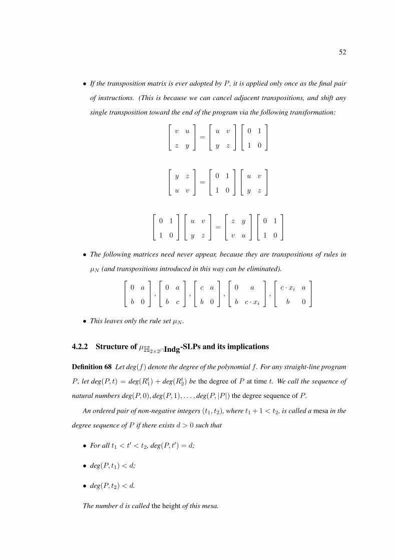
52

• If the transposition matrix is ever adopted by P , it is applied only once as the final pair

of instructions. (This is because we can cancel adjacent transpositions, and shift any

single transposition toward the end of the program via the following transformation: v u

z y

=

u v

y z

0 1

1 0

y z

u v

=

0 1

1 0

u v

y z

0 1

1 0

u v

y z

=

z y

v u

0 1

1 0

• The following matrices need never appear, because they are transpositions of rules in

µN (and transpositions introduced in this way can be eliminated). 0 a

b 0

, 0 a

b c

, c a

b 0

, 0 a

b c · xi

, c · xi a

b 0

• This leaves only the rule set µN .

4.2.2 Structure of µH2×2∩Indg-SLPs and its implications

Definition 68 Let deg(f) denote the degree of the polynomial f . For any straight-line program

P , let deg(P, t) = deg(Rt1) + deg(Rt2) be the degree of P at time t. We call the sequence of

natural numbers deg(P, 0), deg(P, 1), . . . , deg(P, |P |) the degree sequence of P .

An ordered pair of non-negative integers (t1, t2), where t1 + 1 < t2, is called a mesa in the

degree sequence of P if there exists d > 0 such that

• For all t1 < t′ < t2, deg(P, t′) = d;

• deg(P, t1) < d;

• deg(P, t2) < d.

The number d is called the height of this mesa.

53

Fact 69 The operations in Observation 67 that simplify the straight-line program P do not

change the height of any mesa in which the operations are applied.

Now we are ready to show our structural theorem for µH2×2∩Indg-SLPs.

Theorem 70 If a polynomial f is computable by H2×2∩Indg, then there is a µH2×2∩Indg-SLP

P for f with the property that there are no mesas in the degree sequence of P .

Proof. By our assumption, there is some µH2×2∩Indg-SLP P ′ computing f . If P ′ does not

contain any mesas in its degree sequence, then we are done. Otherwise, we will show how to

obtain P from P ′ by a series of transformations. At every step, we turn the current P ′ into

an equivalent µH2×2∩Indg-SLP while reducing the total height of all mesas by at least one.

Ultimately we will obtain a µH2×2∩Indg-SLP P with the desired property. Hence, it suffices

to verify the correctness of a single step.

Let (t1, t2) be the first mesa in the current P ′ and d be its height. There are three cases to

consider.

1. deg(Rt1+11 ) > deg(Rt1+1

2 ).

We claim that the only instruction that can produce this outcome at time t1 + 1 is the

degree-one offsetting rule 3(a). Rule 2 is impossible since it only scales the registers by

a constant factor respectively. Rule 3(b) implies that deg(Rt1+11 ) = deg(Rt11 ); there are

two subcases to consider:

• If deg(Rt11 ) ≥ deg(Rt12 ), then deg(Rt1+11 ) ≤ deg(Rt1+1

2 ), a contradiction to our

assumption that deg(Rt1+11 ) > deg(Rt1+1

2 ).

• If deg(Rt11 ) < deg(Rt12 ), then deg(Rt1+12 ) ≤ deg(Rt12 ). This contradicts our as-

sumption that deg(P, t1) < deg(P, t1 + 1).

For similar reasons, one can show that rules 4(a) and 4(b) are not applicable either. There

are two cases that arise, in dealing with rule 5:

• If deg(Rt11 ) 6= deg(Rt12 ), then under rule 5, deg(Rt1+11 ) = deg(Rt1+1

2 ), which

contradicts our assumption that deg(Rt1+11 ) > deg(Rt1+1

2 );

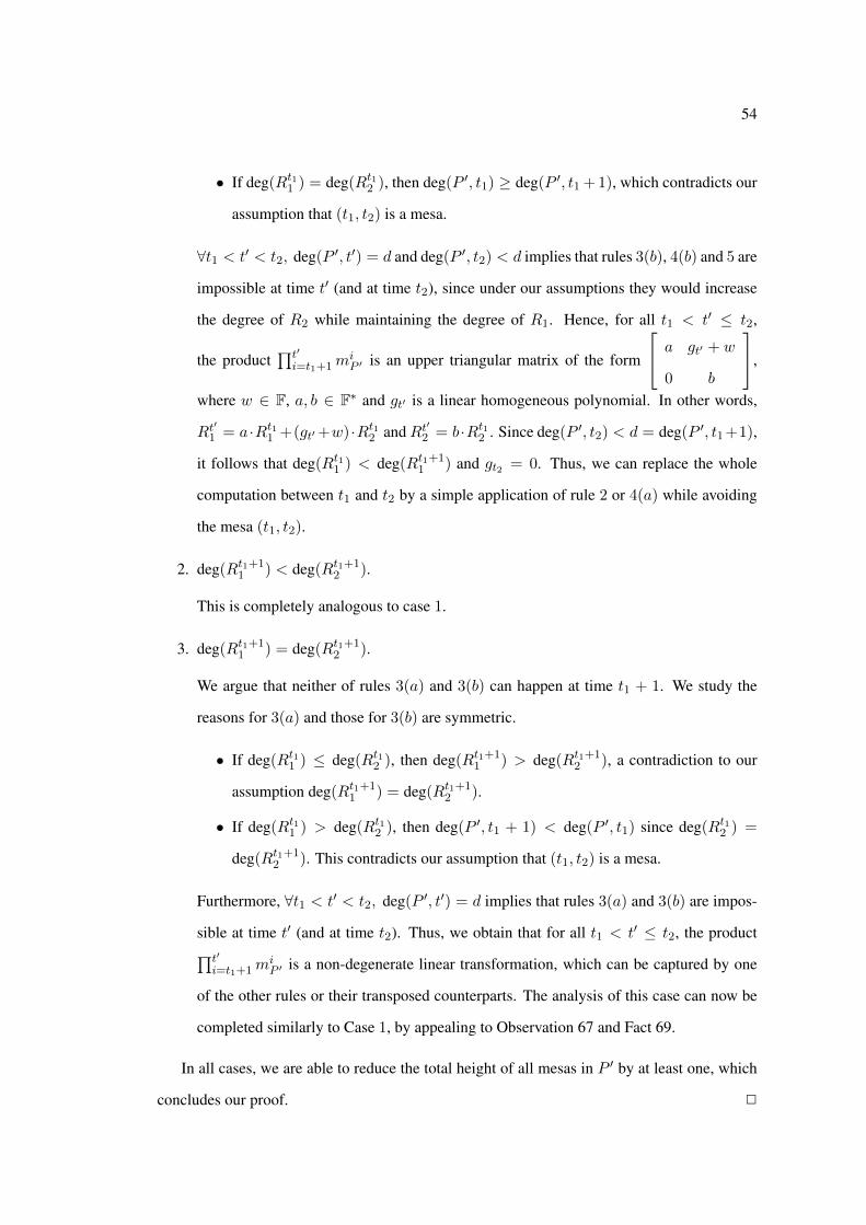
54

• If deg(Rt11 ) = deg(Rt12 ), then deg(P ′, t1) ≥ deg(P ′, t1 + 1), which contradicts our

assumption that (t1, t2) is a mesa.

∀t1 < t′ < t2, deg(P ′, t′) = d and deg(P ′, t2) < d implies that rules 3(b), 4(b) and 5 are

impossible at time t′ (and at time t2), since under our assumptions they would increase

the degree of R2 while maintaining the degree of R1. Hence, for all t1 < t′ ≤ t2,

the product∏t′

i=t1+1miP ′ is an upper triangular matrix of the form

a gt′ + w

0 b

,

where w ∈ F, a, b ∈ F∗ and gt′ is a linear homogeneous polynomial. In other words,

Rt′

1 = a ·Rt11 +(gt′+w) ·Rt12 andRt′

2 = b ·Rt12 . Since deg(P ′, t2) < d = deg(P ′, t1 +1),

it follows that deg(Rt11 ) < deg(Rt1+11 ) and gt2 = 0. Thus, we can replace the whole

computation between t1 and t2 by a simple application of rule 2 or 4(a) while avoiding

the mesa (t1, t2).

2. deg(Rt1+11 ) < deg(Rt1+1

2 ).

This is completely analogous to case 1.

3. deg(Rt1+11 ) = deg(Rt1+1

2 ).

We argue that neither of rules 3(a) and 3(b) can happen at time t1 + 1. We study the

reasons for 3(a) and those for 3(b) are symmetric.

• If deg(Rt11 ) ≤ deg(Rt12 ), then deg(Rt1+11 ) > deg(Rt1+1

2 ), a contradiction to our

assumption deg(Rt1+11 ) = deg(Rt1+1

2 ).

• If deg(Rt11 ) > deg(Rt12 ), then deg(P ′, t1 + 1) < deg(P ′, t1) since deg(Rt12 ) =

deg(Rt1+12 ). This contradicts our assumption that (t1, t2) is a mesa.

Furthermore, ∀t1 < t′ < t2, deg(P ′, t′) = d implies that rules 3(a) and 3(b) are impos-

sible at time t′ (and at time t2). Thus, we obtain that for all t1 < t′ ≤ t2, the product∏t′

i=t1+1miP ′ is a non-degenerate linear transformation, which can be captured by one

of the other rules or their transposed counterparts. The analysis of this case can now be

completed similarly to Case 1, by appealing to Observation 67 and Fact 69.

In all cases, we are able to reduce the total height of all mesas in P ′ by at least one, which

concludes our proof. 2

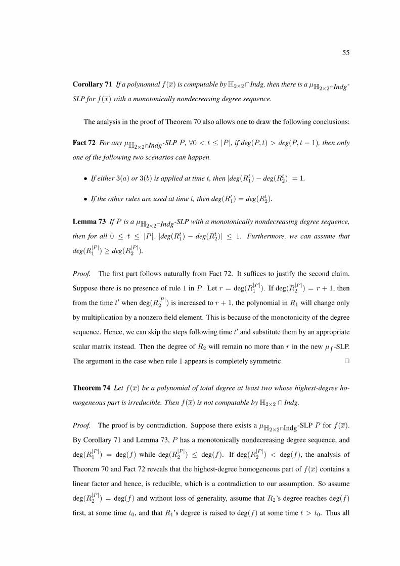
55

Corollary 71 If a polynomial f(x) is computable by H2×2∩Indg, then there is a µH2×2∩Indg-

SLP for f(x) with a monotonically nondecreasing degree sequence.

The analysis in the proof of Theorem 70 also allows one to draw the following conclusions:

Fact 72 For any µH2×2∩Indg-SLP P , ∀0 < t ≤ |P |, if deg(P, t) > deg(P, t − 1), then only

one of the following two scenarios can happen.

• If either 3(a) or 3(b) is applied at time t, then |deg(Rt1)− deg(Rt2)| = 1.

• If the other rules are used at time t, then deg(Rt1) = deg(Rt2).

Lemma 73 If P is a µH2×2∩Indg-SLP with a monotonically nondecreasing degree sequence,

then for all 0 ≤ t ≤ |P |, |deg(Rt1) − deg(Rt2)| ≤ 1. Furthermore, we can assume that

deg(R|P |1 ) ≥ deg(R

|P |2 ).

Proof. The first part follows naturally from Fact 72. It suffices to justify the second claim.

Suppose there is no presence of rule 1 in P . Let r = deg(R|P |1 ). If deg(R

|P |2 ) = r + 1, then

from the time t′ when deg(R|P |2 ) is increased to r + 1, the polynomial in R1 will change only

by multiplication by a nonzero field element. This is because of the monotonicity of the degree

sequence. Hence, we can skip the steps following time t′ and substitute them by an appropriate

scalar matrix instead. Then the degree of R2 will remain no more than r in the new µ∫ -SLP.

The argument in the case when rule 1 appears is completely symmetric. 2

Theorem 74 Let f(x) be a polynomial of total degree at least two whose highest-degree ho-

mogeneous part is irreducible. Then f(x) is not computable by H2×2 ∩ Indg.

Proof. The proof is by contradiction. Suppose there exists a µH2×2∩Indg-SLP P for f(x).

By Corollary 71 and Lemma 73, P has a monotonically nondecreasing degree sequence, and

deg(R|P |1 ) = deg(f) while deg(R

|P |2 ) ≤ deg(f). If deg(R

|P |2 ) < deg(f), the analysis of

Theorem 70 and Fact 72 reveals that the highest-degree homogeneous part of f(x) contains a

linear factor and hence, is reducible, which is a contradiction to our assumption. So assume

deg(R|P |2 ) = deg(f) and without loss of generality, assume that R2’s degree reaches deg(f)

first, at some time t0, and that R1’s degree is raised to deg(f) at some time t > t0. Thus all

56

of the highest-degree monomials in Rt02 come from c · xi · Rt0−11 . For any polynomial g, let

Hd(g) denote the degree-d homogeneous part of polynomial g. An easy induction shows that,

for all t′ such that t0 ≤ t′ ≤ t, Hdeg(f)−1(Rt0−11 ) divides Hdeg(f)(R

t′2 ). By Fact 72, rules

3(a) and 3(b) can not be applied at time t. Since the degree sequence is stable from then on,

they will not happen afterwards either. Hence, by the linearity of the remaining rules, we claim

that ∀t ≤ t′ ≤ |P |, ∃a, b ∈ F∗, Hdeg(f)(Rt′1 ) = aHdeg(f)(R

t′2 ) = bHdeg(f)(R

t−12 ), which

we argued above is divided by Hdeg(f)−1(Rt0−11 ). This is a contradiction to our assumption

that it is irreducible. This concludes our proof. 2

Remark 75 The proof of Theorem 74 reveals that if f(x) is computable by H2×2 ∩ Indg, then

the highest-degree homogeneous part of f(x) can be completely factored into homogeneous

linear polynomials.

4.2.3 Limitation of µH2×2-SLPs

First, by the following lemma, we can assume without loss of generality that for any µH2×2-

SLP P and any inherently degenerate matrix m in P , the entries of m all belong to F.

Proposition 76 If a matrix m ∈ H2×2 ∩ Idg contains at least one entry from H, then m can be

factored into a product of matrices, exactly one of which, denoted as m1, belongs to Idg and

furthermore, all m1’s entries are from F.

Proof. If m has a zero column, then without loss of generality, m is either

a · xi 0

w 0

or

a · xi 0

b · xj 0

where a, b ∈ F∗ and w ∈ F.

a · xi 0

w 0

=

xi 0

0 1

a 0

w 0

while

a · xi 0

b · xj 0

=

xi 0

0 xj

a 0

b 0

. In both cases, we obtain the desired factorization

for m. The case where m has a zero row is symmetric.

For the other cases, it is not hard to see that under our assumption, m can be turned into a

matrix with either a zero column or a zero row via multiplication by a non-degenerate linear

transformation. Our proof is completed by referring to the previous case analysis. 2

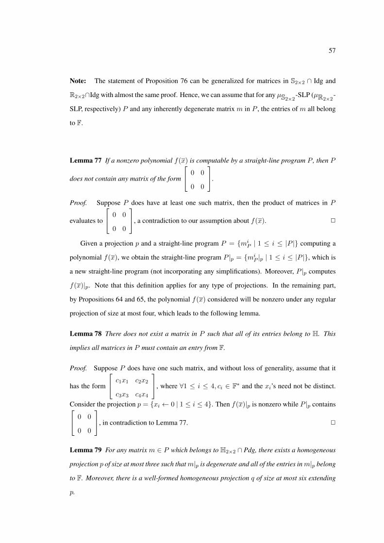
57

Note: The statement of Proposition 76 can be generalized for matrices in S2×2 ∩ Idg and

R2×2∩Idg with almost the same proof. Hence, we can assume that for any µS2×2-SLP (µR2×2

-

SLP, respectively) P and any inherently degenerate matrix m in P , the entries of m all belong

to F.

Lemma 77 If a nonzero polynomial f(x) is computable by a straight-line program P , then P

does not contain any matrix of the form

0 0

0 0

.

Proof. Suppose P does have at least one such matrix, then the product of matrices in P

evaluates to

0 0

0 0

, a contradiction to our assumption about f(x). 2

Given a projection p and a straight-line program P = miP | 1 ≤ i ≤ |P | computing a

polynomial f(x), we obtain the straight-line program P |p = miP |p | 1 ≤ i ≤ |P |, which is

a new straight-line program (not incorporating any simplifications). Moreover, P |p computes

f(x)|p. Note that this definition applies for any type of projections. In the remaining part,

by Propositions 64 and 65, the polynomial f(x) considered will be nonzero under any regular

projection of size at most four, which leads to the following lemma.

Lemma 78 There does not exist a matrix in P such that all of its entries belong to H. This

implies all matrices in P must contain an entry from F.

Proof. Suppose P does have one such matrix, and without loss of generality, assume that it

has the form

c1x1 c2x2

c3x3 c4x4

, where ∀1 ≤ i ≤ 4, ci ∈ F∗ and the xi’s need not be distinct.

Consider the projection p = xi ← 0 | 1 ≤ i ≤ 4. Then f(x)|p is nonzero while P |p contains 0 0

0 0

, in contradiction to Lemma 77. 2

Lemma 79 For any matrix m ∈ P which belongs to H2×2 ∩ Pdg, there exists a homogeneous

projection p of size at most three such thatm|p is degenerate and all of the entries inm|p belong

to F. Moreover, there is a well-formed homogeneous projection q of size at most six extending

p.

58

Proof. The determinant of m, denoted as det(m), is a polynomial of degree at least one.

Since F is algebraically closed, the variety of det(m) is always non-empty and furthermore, by

Lemma 78, det(m) contains at most three variables. This provides us the projection promised

in the first claim. Proposition 64 implies the correctness of the second claim. 2

Definition 80 We call such a well-formed homogeneous projection q as in Lemma 79 a degen-

erating projection for the potentially degenerate matrix m.

Lemma 81 Let f(x) be a polynomial and P be one of its µH2×2-SLPs. Suppose that there

exists 0 < t ≤ |P | such that mtP is a potentially degenerate matrix. Let p be one of its

degenerating projections. Let P ′ = P |p and let Rti(P′) be the contents of Ri at time t in P ′.

Then up to the permutation of the indices, only one of the three following cases will happen.

1. Rt1(P ′) = Rt2(P ′) = 0 and f(x)|p = 0. This is the uninteresting case and we ignore it

in the remainder of the proof.

2. Rt1(P ′) ∈ F∗ and Rt2(P ′) = w ·Rt1(P ′) for some w ∈ F.

3. Rt1(P ′) is a polynomial of degree at least one, Rt2(P ′) = w · Rt1(P ′) for some w ∈ F,

and f(x)|p is divisible by Rt1(P ′).

Proof. Our assumption is thatmtP ′ is a degenerate matrix; let us say that it is

a c

d b

, where

ab − cd=0. Assume for now that c 6= 0. (The case where c = 0 is easier.) Let f and g be

the polynomials given by Rt−11 (P ′) and Rt−1

2 (P ′), respectively. Thus Rt1(P ′) = af + cg and

Rt2(P ′) = (b/c)(af + cg). Thus Rt2(P ′) is a multiple of Rt1(P ′), and an easy induction shows

that Rt1(P ′) will stay as a common factor of both registers from that point on (and thus Rt1(P ′)

also divides f(x)|p. 2

Corollary 82 If f(x)|p is a nonzero irreducible polynomial and the other hypotheses of Lemma

81 hold, then Rt1(P ′) = c · f(x)|p for some c ∈ F∗.

Definition 83 Let f(x), P , mtP and P ′ satisfy the conditions of Lemma 81. If under the degen-

erating projection p, case 2 of Lemma 81 happens, then we call p a cutting projection for mtP

in P . If instead we have case 3, then we call p a finishing projection for mtP in P .

59

Observation 84 Let f(x) be a polynomial such that under any well-formed homogeneous pro-

jection q of size at most six, f(x)|q is always a nonzero irreducible polynomial. Let P be a

µH2×2-SLP for f(x), and let mt

P , p and P ′ be the corresponding objects as in Lemma 81. We

will show how to obtain a µH2×2-SLP for f(x)|p from P as follows:

• If the projection p is a cutting projection for mtP in P , then we can simply ignore the

instructions in P ′ before time t (including the t-th instruction), and concatenate a single

instruction, which is a linear transformation from the initial condition (R01, R

02) = (1, 0)

to the current status (Rt1(P ′), Rt2(P ′)), with the remaining segment of P ′. This produces

a µH2×2-SLP of size at most |P | − t+ 1 for f(x)|p.

• If p is a finishing projection formtP in P , then by Corollary 82, Rt1(P ′) is a nonzero mul-

tiple of f(x)|p and moreover, Rt1(P ′) = a ·Rt−11 (P ′)+b ·Rt−1

2 (P ′), where a, b ∈ H∪F,

since by Lemma 79, all of entries in mtP |p are field elements. We claim that one of a and

b must be a unit. Otherwise, f(x)|p 6= 0 while Rt1(P ′) = 0, a contradiction.Therefore,

we can throw away the portion of P ′ after time t (including the t-th instruction) and

generate R1’s contents Rt1(P ′) by an offsetting matrix m′ at time t, as follows:

We have that Rt1(P ′) is some non-zero multiple of f(x)|p, say Rt1(P ′) = s · f(x)|p. We

also have thatRt1(P ′) = a·Rt−11 (P ′)+b·Rt−1

2 (P ′). If a is a unit, then the desired output

f(x)|p is produced by the assignment Rt1(P ′) ← (a/s) · Rt−11 (P ′) + (b/s) · Rt−1

2 (P ′),

which can be accomplished by a rule of type 3(a) or 4(a) (since we do not care what

value is placed inR2). If b is a unit, then the desired assignment instead is produced by a

transposition of a rule of type 3(b) or 4(b). Thus, in either case, we obtain a µH2×2-SLP

of size at most t+ 1 for f(x)|p.

Definition 85 Let f(x) be a polynomial and P be one of its µH2×2-SLPs. We classify the

potentially degenerate matrices mtP in P , if they do exist, according to the following criterion:

If mtP has at least one finishing projection, then mt

P is good; Otherwise, mtP is bad.

In the same spirit, we can classify inherently degenerate matrices in µH2×2-SLPs. In this

case, we can consider the degenerating projection to be the empty set. The following lemma is

essentially a variant of Lemma 81. Hence, we omit its proof.

60

Lemma 86 Let f(x) be a nonzero polynomial under any well-formed regular projection of size

at most four and P be one of its µH2×2-SLPs. Suppose that there exists 0 < t ≤ |P | such that

mtP is an inherently degenerate matrix. Let w ∈ F. Then up to the permutation of the indices,

only one of the two following cases will happen.

1. Rt1 ∈ F∗ and Rt2 = w ·Rt1 for some w ∈ F.

2. Rt1 has degree at least one, Rt1 = w ·Rt2 and f(x) is divisible by Rt1, where w ∈ F.

Furthermore, If f(x) is a nonzero irreducible polynomial, then in the second case, Rt1 =

c · f(x) where c ∈ F∗.

Definition 87 Let f(x) be as in Lemma 86 and let P be one of its µH2×2-SLPs. Let mt be an

inherently degenerate matrix in P if it exists. If the first case in Lemma 86 happens, then we

say that mt is bad, otherwise, it is good.

Note that the notions of badness and goodness apply only to potentially and inherently

degenerate matrices.

Observation 88 Let p be an arbitrary homogeneous projection and let P ′ = P |p. If mtP is

bad in P , then mtP ′ can not be good in P ′ (This is because, if mt

P is bad, then under any

extension of p, at time t both registers compute field elements which are constant polynomials

with no variables). More precisely, mtP ′ either stays as a bad matrix or becomes an inherently

non-degenerate matrix. Furthermore, inherently non-degenerate matrices will never be turned

into some other type by any projection.

Now we are ready to present our main impossibility theorem of this section.

Theorem 89 If k ≥ 8, then f(x) =∑k

i=1 x2i−1x2i is not computable by H2×2. That is, for

every n, f(x) can not be obtained from IMM2,n under homogeneous projections.

Proof. We prove the theorem by contradiction. Suppose P is a µH2×2-SLP for f(x). We

define the set G of time steps as:

G = t |mtP is a good matrix.

There are two cases to consider.

61

• The first case is that G = ∅. Define the set B similarly as:

B = t |mtP is a bad matrix.

If B is empty as well, then P is indeed a µH2×2∩Indg-SLP. By Fact 60, the highest-

degree homogeneous part of f(x) is irreducible, and by Theorem 74, we have reached

a contradiction. Otherwise, let tB = max(B). Note that, by Proposition 65, the output

at time |P | is a non-zero polynomial under any well-formed regular projection of size

at most six, which means that m|P |P cannot be bad, and hence tB < |P |. Let p be one

of the cutting projections of mtBP . Consider P |p and the polynomial f(x)|p it computes.

Since the size of p is bounded by six, by Proposition 65, f(x)|p is again an irreducible

polynomial and moreover, its degree-two homogeneous part is irreducible. For all t such

that tB ≤ t ≤ |P |, mtP is an inherently non-degenerate matrix. By the first item of

Observation 84, we now have a µH2×2∩Indg-SLP for f(x)|p which is a contradiction to

Theorem 74. Notice that by Proposition 65, the above arguments apply to any polynomial

of the form∑5

i=1 x2i−1x2i + l(x) where l(x) is an arbitrary linear function.

• We assume that G 6= ∅. Let tG = minG. Suppose first that mtGP is an inherently

degenerate matrix. Since mtGP is good, we have by Lemma 86 that, at time tG, register

R1 computes a nonzero multiple of f . Hence by the second item of Observation 84 with

p = ∅, we obtain a new µH2×2-SLP for f(x), consisting of only the matrices before tG

– none of which are good. This brings us back to the first case and a contradiction.

Otherwise, assume that mtGP is a potentially degenerate matrix and let p be one of its

finishing projections of size at most six. Consider P |p and the polynomial f(x)|p it

computes. By the second item of Observation 84, we obtain a new µH2×2-SLP P ′ for

f(x)|p and furthermore, by Observation 88, P ′ does not contain any good matrices.

Hence, this reduces us to the first case, since f(x)|p is of the form∑5

i=1 x2i−1x2i + l(x)

where l(x) is an arbitrary linear function. It is not hard to see that we will arrive at a

contradiction for f(x)|p, which completes our proof.

2

The proof of Theorem 89 leads to the following corollary.

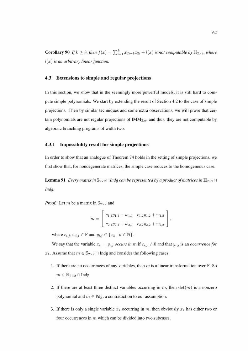
62

Corollary 90 If k ≥ 8, then f(x) =∑k

i=1 x2i−1x2i + l(x) is not computable by H2×2, where

l(x) is an arbitrary linear function.

4.3 Extensions to simple and regular projections

In this section, we show that in the seemingly more powerful models, it is still hard to com-

pute simple polynomials. We start by extending the result of Section 4.2 to the case of simple

projections. Then by similar techniques and some extra observations, we will prove that cer-

tain polynomials are not regular projections of IMM2,n, and thus, they are not computable by

algebraic branching programs of width two.

4.3.1 Impossibility result for simple projections

In order to show that an analogue of Theorem 74 holds in the setting of simple projections, we

first show that, for nondegenerate matrices, the simple case reduces to the homogeneous case.

Lemma 91 Every matrix in S2×2∩ Indg can be represented by a product of matrices in H2×2∩

Indg.

Proof. Let m be a matrix in S2×2 and

m =

c1,1y1,1 + w1,1 c1,2y1,2 + w1,2

c2,1y2,1 + w2,1 c2,2y2,2 + w2,2

,where ci,j , wi,j ∈ F and yi,j ∈ xk | k ∈ N.

We say that the variable xk = yi,j occurs in m if ci,j 6= 0 and that yi,j is an occurrence for

xk. Assume that m ∈ S2×2 ∩ Indg and consider the following cases.

1. If there are no occurrences of any variables, then m is a linear transformation over F. So

m ∈ H2×2 ∩ Indg.

2. If there are at least three distinct variables occurring in m, then det(m) is a nonzero

polynomial and m ∈ Pdg, a contradiction to our assumption.

3. If there is only a single variable xk occurring in m, then obviously xk has either two or

four occurrences in m which can be divided into two subcases.

63

• If xk has two occurrences in m, then these two occurrences can not be placed at the

diagonal or anti-diagonal positions. Hence, without loss of generality, assume that

m has the following form.

m =

w1,1 w1,2

c2,1xk + w2,1 c2,2xk + w2,2

,where c2,1 6= 0 and c2,2 6= 0.

The determinant of m is equal to (c2,2w1,1− c2,1w1,2)xk + (w1,1w2,2−w1,2w2,1),

then by our assumption, c2,2w1,1−c2,1w1,2 = 0. Ifw1,1 = w1,2 = 0, thenm ∈ Idg,

a contradiction to our assumption. If exactly one of them is equal to zero, then

m ∈ Pdg, a contradiction as well. Hence, we can assume that c2,2c2,1=

w1,2

w1,1= d 6= 0.

Then,

m =

w1,1 0

c2,1xk + w2,1 w2,2 − dw2,1

1 d

0 1

w2,2 − dw2,1 6= 0 since det(m) 6= 0.

So

m =

w1,1

c2,10

xk w2,2 − dw2,1

c2,1 0

w2,1

w2,2−dw2,11

1 d

0 1

This verifies that m is a product of matrices in H2×2 ∩ Indg.

• If xk has four occurrences in m, then assume m has the following form.

m =

c1,1xk + w1,1 c1,2xk + w1,2

c2,1xk + w2,1 c2,2xk + w2,2

,where each ci,j 6= 0.

The determinant of m is equal to (c1,1xk + w1,1)(c2,2xk + w2,2) − (c1,2xk +

w1,2)(c2,1xk + w2,1). Because m ∈ Indg, c1,1c2,2 − c1,2c2,1 = 0. Let d =c1,2c1,1

=

c2,2c2,16= 0. Then, there exists u, v ∈ F such that

m =

c1,1xk + w1,1 u

c2,1xk + w2,1 v

1 d

0 1

Obviously the first matrix belongs to Indg because its determinant belongs to F∗.

Hence by the first subcase, it is a product of matrices in H2×2 ∩ Indg, so is m.

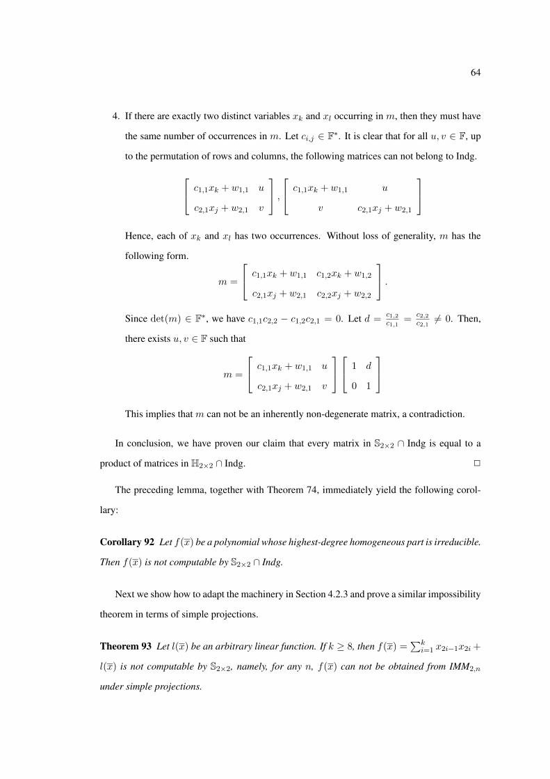
64

4. If there are exactly two distinct variables xk and xl occurring in m, then they must have

the same number of occurrences in m. Let ci,j ∈ F∗. It is clear that for all u, v ∈ F, up

to the permutation of rows and columns, the following matrices can not belong to Indg.

c1,1xk + w1,1 u

c2,1xj + w2,1 v

, c1,1xk + w1,1 u

v c2,1xj + w2,1

Hence, each of xk and xl has two occurrences. Without loss of generality, m has the

following form.

m =

c1,1xk + w1,1 c1,2xk + w1,2

c2,1xj + w2,1 c2,2xj + w2,2

.Since det(m) ∈ F∗, we have c1,1c2,2 − c1,2c2,1 = 0. Let d =

c1,2c1,1

=c2,2c2,16= 0. Then,

there exists u, v ∈ F such that

m =

c1,1xk + w1,1 u

c2,1xj + w2,1 v

1 d

0 1

This implies that m can not be an inherently non-degenerate matrix, a contradiction.

In conclusion, we have proven our claim that every matrix in S2×2 ∩ Indg is equal to a

product of matrices in H2×2 ∩ Indg. 2

The preceding lemma, together with Theorem 74, immediately yield the following corol-

lary:

Corollary 92 Let f(x) be a polynomial whose highest-degree homogeneous part is irreducible.

Then f(x) is not computable by S2×2 ∩ Indg.

Next we show how to adapt the machinery in Section 4.2.3 and prove a similar impossibility

theorem in terms of simple projections.

Theorem 93 Let l(x) be an arbitrary linear function. If k ≥ 8, then f(x) =∑k

i=1 x2i−1x2i +

l(x) is not computable by S2×2, namely, for any n, f(x) can not be obtained from IMM2,n

under simple projections.

65

Proof. [Proof sketch] We prove the theorem via contradiction. Suppose there is a µS2×2-SLP

P for f(x).

Similar to Lemma 78, we prove the following lemma.

Lemma 94 There does not exist a matrix m in P such that each entry of m contains a distinct

variable. This implies that all matrices in P must contain at most three variables.

Proof. Suppose the statement is not true, and without loss of generality,

m =

c1x1 − w1 c2x2 − w2

c3x3 − w3 c4x4 − w4

,

where ∀1 ≤ i ≤ 4, ci ∈ F∗, wi ∈ F and the xis are all distinct.

Consider the projection p = xi ← wici| 1 ≤ i ≤ 4. Then f(x)|p is nonzero while P |p

contains

0 0

0 0

. By Propositions 64 and 65, f(x) is nonzero under any regular projection

of size at most four. Thus by Lemma 77, we have reached a contradiction. 2

A direct consequence of Lemma 94 is an analogue of Lemma 79. The proof of the following

lemma proceeds in the same way as that of Lemma 79, so we omit it here.

Lemma 95 For any matrix m ∈ P which belongs to S2×2 ∩ Pdg, there exists a homogeneous

projection p of size at most three such thatm|p is degenerate and all of the entries inm|p belong

to F. Moreover, there is a well-formed homogeneous projection q of size at most six extending

p.

The notions of degenerating projections, and of good and bad matrices, thus carry over also

to the setting of simple projections, and the rest of the proof follows exactly as in Section 4.2.3.

2

4.3.2 Impossibility result for regular projections

Let m ∈ R2×2 be of the following form:

m =

l1,1 + w1,1 l1,2 + w1,2

l2,1 + w2,1 l2,2 + w2,2

.

66

where wi,j ∈ F and the li,j’s are homogeneous linear forms in ∑n

k=1 ckxk | n ∈ N, ck ∈ F.

We will pay attention to the rank of the subspace spanned by li,j | i, j ∈ 1, 2, denoted

as r(m), which in some sense characterizes the number of “independent variables” among the

li,j’s.

The following lemma illustrates the sense in which we can treat linearly-independent ho-

mogeneous linear forms as independent variables.

Lemma 96 Let l1, l2, . . . , lk be k linearly independent homogeneous linear forms, and let

w1, . . . , wk be elements of F. Then there is a regular projection p of size k such that, for

all i, li|p = wi. (Thus we can think of p as a “projection” of the form li ← wi.)

Proof. The homogeneous linear form l1 is of the form∑n

j=1 cjxj , where each cj ∈ F∗. Start

building the projection p with the rule x1 ← (w1 −∑n

j=2 cjxj)/c1. This clearly has the effect

that l1|p = w1. If k = 1, then the construction ends here.

Otherwise, let l2 =∑n′

j=1 djyj , where each dj ∈ F∗. If the variable x1 appears as one of

the variables yj , then replace x1 with the expression (w1 −∑n

j=2 cjxj)/c1 and simplify. By

linear independence, there must still be some variable remaining in the resulting expression.

Without loss of generality, let the resulting expression be of the form∑n′′

j=2 ajxj . Then we add

a new rule x2 ← (w2 −∑n′′

j=3 ajxj)/a2 (and if this variable x2 occurs in the right-hand-side

of the rule for x1, then substitute this expression in for x2 in that rule, and simplify). At this

point, we have l1|p = w1 and l2|p = w2.

We continue in this way for all of the remaining linear forms. The crucial observation is

that there will always be a variable in each linear form lj |p when we first consider it, because

of linear independence. 2

Our next lemma is a generalization of Lemma 91.

Lemma 97 Every matrix m in R2×2 ∩ Indg can be represented by a product of matrices in

H2×2 ∩ Indg.

Proof. The correctness of the following claim is easy to verify.

If r(m) = 0, 3 or 4, then the proof is completely analogous to the corresponding cases in

67

Lemma 91, where we do our case analysis based on r(m) instead of the number of variables

that occur in m.

If r(m) = 1, then there exists a homogeneous linear form l such that all li,js in m are

multiples of l. By treating l as a single variable, the analysis of the third case in Lemma

91 reveals that m is a product of matrices from H2×2 ∩ Indg as well as matrices having the

following form: c 0

l c′

, c l

0 c′

.Thus the case when r(m) = 1 is completed by appealing to the following claim:

Claim 98 Any matrix having the following form can be expressed as the product of matrices

in H2×2 ∩ Indg. c 0

l c′

, c l

0 c′

where c, c′ ∈ F∗ and l ∈ L.

Proof. We prove the claim by induction on the number of variables appearing in l. If l contains

at most one variable, then the claim follows from Lemma 91.

Otherwise, l is of the form dx1 + l′. Observe that c 0

l c′

=

c/d 0

x1 1

× d 0

l′ c′

.(The other case is similar.) The claim now follows by induction. 2

If r(m) = 2, then let l1, l2 ∈ li,j | i, j ∈ 1, 2 be a basis. If every li,j is a multiple

of either l1 or l2, then the proof of the fourth case of Lemma 91 provides us a contradiction.

Thus, we only need to consider the case where there is at least one l′ ∈ li,j | i, j ∈ 1, 2

and c, c′ ∈ F∗ such that l′ = cl1 + c′l2, which means that l′ is a non-trivial linear combination

of l1 and l2. Therefore, without loss of generality, we assume that m has the following form.

m =

l1 + w1,1 l2 + w1,2

cl1 + c′l2 + w2,1 dl1 + d′l2 + w2,2

.where c, c′ ∈ F∗, d, d′ ∈ F.

68

But then the degree-two homogeneous part of det(m) is equal to dl21 + (d′ − c)l1l2 − c′l22,

which is nonzero since c′ 6= 0. This contradicts our assumption that m ∈ Indg. 2

The preceding lemma, together with Theorem 74, immediately yield the following corol-

lary:

Corollary 99 Let f(x) be a polynomial whose highest-degree homogeneous part is irreducible.

Then f(x) is not computable by R2×2 ∩ Indg.

Now we are ready to prove our main theorem.

Theorem 100 (Theorem 11 restated) If k ≥ 8, then f(x) =∑k

i=1 x2i−1x2i is not com-

putable by R2×2, namely, for any n, f(x) can not be obtained from IMM2,n under regular

projections.

Proof. [Proof sketch] The proof is by contradiction. Suppose P is a µR2×2-SLP for f(x).

By Propositions 64 and 65, f(x) is nonzero under any regular projection of size at most

four, which leads to the following lemma.

Lemma 101 For any potentially degenerate matrix mtP in P , r(mt

P ) ≤ 3.

Proof. Suppose r(mtP ) = 4, then there exists a regular projection p of size four such that

∀1 ≤ i, j ≤ 2, li,j = −wi,j . In other words, mtP |p =

0 0

0 0

. By Lemma 77, we have

reached a contradiction to the aforementioned property of f(x). 2

Lemma 102 Any potentially degenerate matrix mtP in P has a regular projection p of size at

most three such that mtP |p is degenerate and all of the entries in m|p belong to F. Moreover,

there is a well-formed regular projection q of size at most six extending p.

Proof. det(mtP ) is a polynomial of degree at least one. by Lemma 101, after some suitable

linear transformation, det(mtP ) can be viewed as a polynomial in at most three “new” variables

that are linear forms in terms of the original set of variables. Since F is algebraically closed,

this provides us the desired projection p. The second part of the claim follows from Proposition

64. 2

69

By Lemma 102, we can define degenerating projections in terms of well-formed regular

projections. Note that the proofs of Lemma 81 and Corollary 82 hold, regardless of the type

of projections. Thus we can also extend the definitions of cutting and finishing projections to

well-formed regular projections. The following observation is a slight variant of Observation

84.

Observation 103 Let f(x) be a polynomial such that under any well-formed regular projection

q of size at most six, f(x)|q is always a nonzero irreducible polynomial. Let P be a µR2×2-

SLP for f(x) and let mtP be a potentially degenerate matrix in P . Let p be one of degenerating

regular projections of mtP and let P ′ = P |p. Then, a µR2×2

-SLP can be constructed for

f(x)|p.

• If p is a cutting projection for mtP in P , this case is identical to the first case in Obser-

vation 84.

• If p is a finishing projection for mtP in P , this case is identical to the second case in

Observation 84.

Now the remaining part of proof proceeds exactly as in Section 4.2.3, since it does not

depend on the type of underlying projections at all, namely, regardless of whether they are

homogeneous, simple or regular. 2

70

References

[AAB+99] A. Ambainis, E. Allender, D. A. M. Barrington, S. Datta, and H. LeThanh.Bounded depth arithmetic circuits: Counting and closure. In Proc. of Interna-tional Conference on Automata, Languages, and Programming (ICALP), number1644 in Lecture Notes in Computer Science, pages 149–158. Springer, 1999.

[AAD00] Manindra Agrawal, Eric Allender, and Samir Datta. On TC0, AC0, and arith-metic circuits. Journal of Computer and System Sciences, 60(2):395–421, 2000.

[AB09] Sanjeev Arora and Boaz Barak. Computational Complexity, a modern approach.Cambridge University Press, 2009.

[ABFR94] James Aspnes, Richard Beigel, Merrick L. Furst, and Steven Rudich. The ex-pressive power of voting polynomials. Combinatorica, 14(2):135–148, 1994.

[ABKPM09] Eric Allender, Peter Burgisser, Johan Kjeldgaard-Pedersen, and Peter Bro Mil-tersen. On the complexity of numerical analysis. SIAM Journal on Computing,38(5):1987–2006, 2009.

[ACR98] Alexander E. Andreev, Andrea E. F. Clementi, and Jose D. P. Rolim. A newgeneral derandomization method. Journal of the ACM, 45(1):179–213, 1998.

[ACR99] Alexander E. Andreev, Andrea E. F. Clementi, and Jose D. P. Rolim. Worst-casehardness suffices for derandomization: A new method for hardness-randomnesstrade-offs. Theoretical Computer Science, 221(1-2):3–18, 1999.

[ACRT99] Alexander E. Andreev, Andrea E. F. Clementi, Jose D. P. Rolim, and Luca Tre-visan. Weak random sources, hitting sets, and BPP simulations. SIAM Journalon Computing, 28(6):2103–2116, 1999.

[Adl78] Leonard M. Adleman. Two theorems on random polynomial time. In Proc.IEEE Symp. on Found. of Comp. Sci. (FOCS), pages 75–83, 1978.

[ADR05] Eric Allender, Samir Datta, and Sambuddha Roy. Topology inside NC11. InProc. IEEE Conf. on Computational Complexity, pages 298–307, 2005.

[AG94] Eric Allender and Vivek Gore. A uniform circuit lower bound for the permanent.SIAM Journal on Computing, 23(5):1026–1049, 1994.

[AH94] Eric Allender and Ulrich Hertrampf. Depth reduction for circuits of unboundedfan-in. Information and Computation, 112(2):217–238, 1994.

[AHM+08] Eric Allender, Lisa Hellerstein, Paul McCabe, Toniann Pitassi, and Michael E.Saks. Minimizing disjunctive normal form formulas and AC0 circuits given atruth table. SIAM Journal on Computing, 38(1):63–84, 2008.

71

[AJMV98] Eric Allender, Jia Jiao, Meena Mahajan, and V. Vinay. Non-commutative arith-metic circuits: Depth reduction and size lower bounds. Theor. Comput. Sci.,209(1-2):47–86, 1998.

[Ajt83] Miklos Ajtai. σ11-formulae on finite structures. Annals of Pure and Applied

Logic, 24:1–48, 1983.

[AK97] Vikraman Arvind and Johannes Kobler. On resource-bounded measure andpseudorandomness. Proc. Conference on Foundations of Software Technologyand Theoretical Computer Science (FST&TCS), pages 235–249, 1997.

[AK10] Eric Allender and Michal Koucky. Amplifying lower bounds by means of self-reducibility. Journal of the ACM, 57(3), 2010.

[All89] Eric Allender. A note on the power of threshold circuits. In Proc. IEEE Symp.on Found. of Comp. Sci. (FOCS), pages 580–584, 1989.

[All96] Eric Allender. Circuit complexity before the dawn of the new millennium. InProc. Conference on Foundations of Software Technology and Theoretical Com-puter Science (FST&TCS), pages 1–18, 1996.

[All99] Eric Allender. The permanent requires large uniform threshold circuits. ChicagoJournal of Theorerical Computer Science, 1999, 1999.

[All04] Eric Allender. Arithmetic circuits and counting complexity classes. InJ. Krajıcek, editor, Complexity of Computations and Proofs, volume 13 ofQuaderni di Matematica, pages 33–72. Seconda Universita di Napoli, 2004.

[All10] Eric Allender. New surprises from self-reducibility. In F. Ferreira, H. Guerra,E. Mayordomo, and J. Rasga, editors, Programs, Proofs, Processes, Conferenceon Computability in Europe, pages 1–5. Centre for Applied Mathematics andInformation Technology, Dept. of Mathematics, University of Azores, 2010.

[AV08] Manindra Agrawal and V. Vinay. Arithmetic circuits: A chasm at depth four. InProc. IEEE Symp. on Found. of Comp. Sci. (FOCS), pages 67–75, 2008.

[AW93] Eric W. Allender and Klaus W. Wagner. Counting hierarchies: polynomial timeand constant depth circuits. In G. Rozenberg and A. Salomaa, editors, CurrentTrends in Theoretical Computer Science, World Scientific Series in ComputerScience, pages 469–483. World Scientific Press, 1993.

[Bar85] David A. Barrington. Width-3 permutation branching programs. Technical Re-port Technical Memorandum MIT/LCS/TM-293, MIT, 1985.

[Bar89] David A. Barrington. Bounded-width polynomial-size branching programs rec-ognize exactly those languages in NC1. Journal of Computer and System Sci-ences, 38(1):150–164, 1989.

[Bar92] David A. Mix Barrington. Quasipolynomial size circuit classes. In Proc. IEEEConf. on Structure in Complexity Theory, pages 86–93, 1992.

[Bea] Paul Beame. A switching lemma primer. Manuscripthttp://www.cs.washington.edu/homes/beame/primer.ps.

72

[Bei94] Richard Beigel. When do extra majority gates help? polylog(n) majority gatesare equivalent to one. Computational Complexity, 4:314–324, 1994.

[BF99] Harry Buhrman and Lance Fortnow. One-sided versus two-sided error in prob-abilistic computation. Proc. of Symp. on Theo. Aspects of Comp. Sci. (STACS),pages 100–109, 1999.

[BFNW93] Laszlo Babai, Lance Fortnow, Noam Nisan, and Avi Wigderson. BPP has subex-ponential time simulations unless EXPTIME has publishable proofs. Computa-tional Complexity, 3:307–318, 1993.

[BH89] Paul Beame and Johan Hastad. Optimal bounds for decision problems on thecrcw pram. Journal of the ACM, 36(3):643–670, 1989.

[BIS90] David A. Mix Barrington, Neil Immerman, and Howard Straubing. On unifor-mity within NC11. Journal of Computer and System Sciences, 41(3):274–306,1990.

[BM84] Manuel Blum and Silvio Micali. How to generate cryptographically strong se-quences of pseudo-random bits. SIAM Journal on Computing, 13(4):850–864,1984.

[BOC88] Michael Ben-Or and Richard Cleve. Computing algebraic formulas using a con-stant number of registers. In Proc. ACM Symp. on Theory of Computing (STOC),pages 254–257, 1988.

[BOC92] Michael Ben-Or and Richard Cleve. Computing algebraic formulas using a con-stant number of registers. SIAM Journal on Computing, 21(1):54–58, 1992.

[BT88] David A. Mix Barrington and Denis Therien. Finite monoids and the fine struc-ture of nc1. Journal of the ACM, 35(4):941–952, 1988.

[BT94] Richard Beigel and Jun Tarui. On ACC. Computational Complexity, 4:350–366,1994.

[BTT92] Richard Beigel, Jun Tarui, and Seinosuke Toda. On probabilistic acc circuitswith an exact-threshold output gate. In International Symposium on Algorithmsand Computation, pages 420–429, 1992.

[Bur00] Peter Burgisser. Cook’s versus valiant’s hypothesis. Theoretical Computer Sci-ence, 235(1):71–88, 2000.

[Bus93] Samuel R. Buss. Algorithms for boolean formula evaluation and for tree-contraction. In P. Clote and J. Krajıcek, editors, Proof Theory, Complexity, andArithmetic, pages 95–115. Oxford University Press, 1993.

[Cai89] Jinyi Cai. With probability one, a random oracle separates PSPACE fromthe polynomial-time hierarchy. Journal of Computer and System Sciences,38(1):68–85, 1989.

[CMTV98] H. Caussinus, P. McKenzie, D. Therien, and H. Vollmer. Nondeterministic NC0

computation. Journal of Computer and System Sciences, 57:200–212, 1998.

73

[CSV84] Ashok K. Chandra, Larry J. Stockmeyer, and Uzi Vishkin. Constant depth re-ducibility. SIAM Journal on Computing, 13(2):423–439, 1984.

[DS05] Zeev Dvir and Amir Shpilka. Locally decodable codes with 2 queries and poly-nomial identity testing for depth 3 circuits. In Proc. ACM Symp. on Theory ofComputing (STOC), pages 592–601, 2005.

[DSY09] Zeev Dvir, Amir Shpilka, and Amir Yehudayoff. Hardness-randomness trade-offs for bounded depth circuits. SIAM Journal on Computing, 39(4):1279–1293,2009.

[FF91] Joan Feigenbaum and Lance Fortnow. On the random-self-reducibility of com-plete sets. In Structure in Complexity Theory Conference, pages 124–132, 1991.

[FSS84] Merrick L. Furst, James B. Saxe, and Michael Sipser. Parity, circuits, and thepolynomial-time hierarchy. Mathematical Systems Theory, 17(1):13–27, 1984.

[GGH+07] Shafi Goldwasser, Dan Gutfreund, Alexander Healy, Tali Kaufman, and Guy N.Rothblum. Verifying and decoding in constant depth. In Proc. ACM Symp. onTheory of Computing (STOC), pages 440–449, 2007.

[GK98] Dima Grigoriev and Marek Karpinski. An exponential lower bound for depth 3arithmetic circuits. In Proc. ACM Symp. on Theory of Computing (STOC), pages577–582, 1998.

[GR00] Dima Grigoriev and Alexander A. Razborov. Exponential lower bounds fordepth 3 arithmetic circuits in algebras of functions over finite fields. ApplicableAlgebra in Engineering, Communication and Computing, 10(6):465–487, 2000.

[Gro94] Vince Grolmusz. A weight-size trade-off for circuits with modm gates. In Proc.ACM Symp. on Theory of Computing (STOC), pages 68–74, 1994.

[GV04] Dan Gutfreund and Emanuele Viola. Fooling parity tests with parity gates.APPROX-RANDOM, pages 381–392, 2004.

[GVW00] Oded Goldreich, Salil P. Vadhan, and Avi Wigderson. Simplified derandomiza-tion of BPP using a hitting set generator. Electronic Colloquium on Computa-tional Complexity, 7(4), 2000.

[GW99] Oded Goldreich and Avi Wigderson. Improved derandomization of BPP using ahitting set generator. RANDOM-APPROX, pages 131–137, 1999.

[HAB02] William Hesse, Eric Allender, and David A. Mix Barrington. Uniform constant-depth threshold circuits for division and iterated multiplication. Journal of Com-puter and System Sciences, 65(4):695–716, 2002.

[Han06] Kristoffer Arnsfelt Hansen. Constant width planar computation characterizesACC0. Theory of Computing Systems, 39(1):79–92, 2006.

[Has86] Johan Hastad. Almost optimal lower bounds for small depth circuits. In Proc.ACM Symp. on Theory of Computing (STOC), pages 6–20, 1986.

[HG91] Johan Hastad and Mikael Goldmann. On the power of small-depth thresholdcircuits. Computational Complexity, 1:113–129, 1991.

74

[HK09] Kristoffer Arnsfelt Hansen and Michal Koucky. A new characterization of ACC0

and probabilistic CC0. In Proc. IEEE Conf. on Computational Complexity, pages27–34, 2009.

[HM04] Kristoffer Arnsfelt Hansen and Peter Bro Miltersen. Some meet-in-the-middlecircuit lower bounds. In Proc. of Math. Foundations of Comp. Sci. (MFCS),pages 334–345, 2004.

[HMP+93] Andras Hajnal, Wolfgang Maass, Pavel Pudlak, Mario Szegedy, and GyorgyTuran. Threshold circuits of bounded depth. Journal of Computer and SystemSciences, 46(2):129–154, 1993.

[IKW02] Russell Impagliazzo, Valentine Kabanets, and Avi Wigderson. In search of aneasy witness: exponential time vs. probabilistic polynomial time. Journal ofComputer and System Sciences, 65(4):672–694, 2002.

[Imm89] Neil Immerman. Expressibility and parallel complexity. SIAM Journal on Com-puting, 18(3):625–638, 1989.

[Imp95] Russell Impagliazzo. Hard-core distributions for somewhat hard problems.Proc. IEEE Symp. on Found. of Comp. Sci. (FOCS), pages 538–545, 1995.

[IPS97] Russell Impagliazzo, Ramamohan Paturi, and Michael E. Saks. Size-depthtradeoffs for threshold circuits. SIAM Journal on Computing, 26(3):693–707,1997.

[ISW06] Russell Impagliazzo, Ronen Shaltiel, and Avi Wigderson. Reducing the seedlength in the Nisan-Wigderson generator. Combinatorica, 26(6):647–681, 2006.

[IW97] Russell Impagliazzo and Avi Wigderson. P = BPP if E requires exponentialcircuits: Derandomizing the XOR lemma. Proc. ACM Symp. on Theory of Com-puting (STOC), pages 220–229, 1997.

[IW01] Russell Impagliazzo and Avi Wigderson. Randomness vs time: Derandomiza-tion under a uniform assumption. Journal of Computer and System Sciences,63(4):672–688, 2001.

[Jan08] Maurice J. Jansen. Lower bounds for syntactically multilinear algebraic branch-ing programs. In Proc. of Math. Foundations of Comp. Sci. (MFCS), number5162 in Lecture Notes in Computer Science, pages 407–418. Springer, 2008.

[JR09] Maurice J. Jansen and B. V. Raghavendra Rao. Simulation of arithmetical cir-cuits by branching programs with preservation of constant width and syntacticmultilinearity. In CSR, number 5675 in Lecture Notes in Computer Science,pages 179–190. Springer, 2009.

[Jun85] H. Jung. Depth efficient transformations of arithmetic into Boolean circuits. InProc. FCT, number 199 in Lecture Notes in Computer Science, pages 167–173.Springer, 1985.

[Kab02] Valentine Kabanets. Derandomization: a brief overview. Bulletin of the EATCS,76:88–103, 2002.

75

[KI04] Valentine Kabanets and Russell Impagliazzo. Derandomizing polynomial iden-tity tests means proving circuit lower bounds. Computational Complexity, 13(1-2):1–46, 2004.

[Kil88] Joe Kilian. Founding cryptography on oblivious transfer. In Proc. ACM Symp.on Theory of Computing (STOC), pages 20–31, 1988.

[KL80] Richard M. Karp and Richard J. Lipton. Some connections between nonuniformand uniform complexity classes. In Proc. ACM Symp. on Theory of Computing(STOC), pages 302–309, 1980.

[KMSV10] Zohar Shay Karnin, Partha Mukhopadhyay, Amir Shpilka, and Ilya Volkovich.Deterministic identity testing of depth-4 multilinear circuits with bounded topfan-in. In Proc. ACM Symp. on Theory of Computing (STOC), pages 649–658,2010.

[KP94] Matthias Krause and Pavel Pudlak. On the computational power of depth 2 cir-cuits with threshold and modulo gates. In Proc. ACM Symp. on Theory of Com-puting (STOC), pages 48–57, 1994.

[KP09] Pascal Koiran and Sylvain Perifel. A superpolynomial lower bound on the sizeof uniform non-constant-depth threshold circuits for the permanent. In Proc.IEEE Conf. on Computational Complexity, pages 35–40, 2009.

[KS01] Adam Klivans and Daniel A. Spielman. Randomness efficient identity testing ofmultivariate polynomials. In Proc. ACM Symp. on Theory of Computing (STOC),pages 216–223, 2001.

[KS06] Neeraj Kayal and Nitin Saxena. Polynomial identity testing for depth 3 circuits.In Proc. IEEE Conf. on Computational Complexity, pages 9–17, 2006.

[KS08] Zohar Shay Karnin and Amir Shpilka. Black box polynomial identity testing ofgeneralized depth-3 arithmetic circuits with bounded top fan-in. In Proc. IEEEConf. on Computational Complexity, pages 280–291, 2008.

[KS09] Neeraj Kayal and Shubhangi Saraf. Blackbox polynomial identity testing fordepth 3 circuits. In Proc. IEEE Symp. on Found. of Comp. Sci. (FOCS), pages198–207, 2009.

[KvM02] Adam Klivans and Dieter van Melkebeek. Graph nonisomorphism has subexpo-nential size proofs unless the polynomial-time hierarchy collapses. SIAM Jour-nal on Computing, 31(5):1501–1526, 2002.

[KVVY93] Ravi Kannan, H. Venkateswaran, V. Vinay, and Andrew Chi-Chih Yao. A circuit-based proof of toda’s theorem. Information and Computation, 104(2):271–276,1993.

[Lip91] Richard J. Lipton. New directions in testing. In Distributed Computing andCryptography, volume 2 of DIMACS Series in Discrete Mathematics and Theo-retical Computer Science, pages 191–202. AMS, 1991.

[LZ77] R. Lipton and Y. Zalcstein. Word problems solvable in logspace. Journal of theACM, 24:522–526, 1977.

76

[MC87] Pierre McKenzie and Stephen A. Cook. The parallel complexity of Abelian per-mutation group problems. SIAM Journal on Computing, 16(5):880–909, 1987.

[MR09] Meena Mahajan and B. V. Raghavendra Rao. Small-space analogues of valiant’sclasses. In FCT, number 5699 in Lecture Notes in Computer Science, pages250–261. Springer, 2009.

[MSS11] M. Mahajan, N. Saurabh, and K. Sreenivasaiah. Counting paths in planar width2 branching programs. Manuscript, 2011.

[MV97] M. Mahajan and V. Vinay. Determinant: Combinatorics, algorithms, and com-plexity. Chicago Journal of Theoretical Computer Science, (5), 1997.

[MV05] Peter Bro Miltersen and N. V. Vinodchandran. Derandomizing Arthur-Merlingames using hitting sets. Computational Complexity, 14(3):256–279, 2005.

[Nis91] Noam Nisan. Lower bounds for non-commutative computation (extended ab-stract). In Proc. ACM Symp. on Theory of Computing (STOC), pages 410–418,1991.

[NR04] Moni Naor and Omer Reingold. Number-theoretic constructions of efficientpseudo-random functions. Journal of the ACM, 51(2):231–262, 2004.

[NW94] Noam Nisan and Avi Wigderson. Hardness vs randomness. Journal of Computerand System Sciences, 49(2):149–167, 1994.

[NW97] Noam Nisan and Avi Wigderson. Lower bounds on arithmetic circuits via partialderivatives. Computational Complexity, 6(3):217–234, 1997.

[PS88] Ian Parberry and Georg Schnitger. Parallel computation with threshold func-tions. Journal of Computer and System Sciences, 36(3):278–302, 1988.

[PS89] Ian Parberry and Georg Schnitger. Relating boltzmann machines to conventionalmodels of computation. Neural Networks, 2(1):59–67, 1989.

[Raz87] Alexander Razborov. Lower bounds on the size of bounded-depth networks overa complete basis with logical addition. Mathematical Notes of the Academy ofSciences. of the USSR, 41(4):333–338, 1987.

[Raz92] Alexander A. Razborov. On small depth threshold circuits. In ScandinavianWorkshop on Algorithm Theory, pages 42–52, 1992.

[Raz95] Alexander Razborov. Bounded arithmetic and lower bounds in boolean com-plexity. Feasible Mathematics II, pages 344–386, 1995.

[Raz09] Ran Raz. Multi-linear formulas for permanent and determinant are of super-polynomial size. Journal of the ACM, 56(2), 2009.

[Raz10] Ran Raz. Elusive functions and lower bounds for arithmetic circuits. Theory ofComputing, 6(1):135–177, 2010.

[Rob93] D. Robinson. Parallel algorithms for group word problems. PhD thesis, Univ.of California, San Diego, 1993.

77

[RR97] Alexander A. Razborov and Steven Rudich. Natural proofs. Journal of Com-puter and System Sciences, 55(1):24–35, 1997.

[RW93] Alexander A. Razborov and Avi Wigderson. nΩ(logn) lower bounds on the size ofdepth-3 threshold circuits with and gates at the bottom. Information ProcessingLetters, 45(6):303–307, 1993.

[RY09] Ran Raz and Amir Yehudayoff. Lower bounds and separations for constant depthmultilinear circuits. Computational Complexity, 18(2):171–207, 2009.

[Sch80] Jacob T. Schwartz. Fast probabilistic algorithms for verification of polynomialidentities. Journal of the ACM, 27(4):701–717, 1980.

[Sha81] Adi Shamir. On the generation of cryptographically strong pseudo-random se-quences. Proc. of International Conference on Automata, Languages, and Pro-gramming (ICALP), pages 544–550, 1981.

[She07] Alexander A. Sherstov. Separating AC0 from depth-2 majority circuits. In Proc.ACM Symp. on Theory of Computing (STOC), pages 294–301, 2007.

[Shp01] Amir Shpilka. Lower bounds for small depth arithmetic and Boolean circuits.PhD thesis, Hebrew University, 2001.

[Sit96] Meera Sitharam. Approximation from linear spaces and applications to com-plexity. Electronic Colloquium on Computational Complexity, 3(30), 1996.

[Smo87] Roman Smolensky. Algebraic methods in the theory of lower bounds for booleancircuit complexity. In Proc. ACM Symp. on Theory of Computing (STOC), pages77–82, 1987.

[SS09] Nitin Saxena and C. Seshadhri. An almost optimal rank bound for depth-3 iden-tities. In Proc. IEEE Conf. on Computational Complexity, pages 137–148, 2009.

[SS10] Nitin Saxena and C. Seshadhri. From sylvester-gallai configurations to rankbounds: Improved black-box identity test for depth-3 circuits. In Proc. IEEESymp. on Found. of Comp. Sci. (FOCS), pages 21–29, 2010.

[SS11] Nitin Saxena and C. Seshadhri. Blackbox identity testing for bounded top fanindepth-3 circuits: the field doesn’t matter. In Proc. ACM Symp. on Theory ofComputing (STOC), 2011. To appear.

[STV01] Madhu Sudan, Luca Trevisan, and Salil P. Vadhan. Pseudorandom generatorswithout the XOR lemma. Journal of Computer and System Sciences, 62(2):236–266, 2001.

[SU05] Ronen Shaltiel and Christopher Umans. Simple extractors for all min-entropiesand a new pseudorandom generator. Journal of the ACM, 52(2):172–216, 2005.

[SV10] Ronen Shaltiel and Emanuele Viola. Hardness amplification proofs require ma-jority. SIAM Journal on Computing, 39(7):3122–3154, 2010.

[SW01] Amir Shpilka and Avi Wigderson. Depth-3 arithmetic circuits over fields ofcharacteristic zero. Computational Complexity, 10(1):1–27, 2001.

78

[Tar93] Jun Tarui. Probablistic polynomials, AC0 functions, and the polynomial-timehierarchy. Theoretical Computer Science, 113(1):167–183, 1993.

[Tod89] Seinosuke Toda. On the computational power of pp and +p. In Proc. IEEE Symp.on Found. of Comp. Sci. (FOCS), pages 514–519, 1989.

[Uma03] Christopher Umans. Pseudo-random generators for all hardnesses. Journal ofComputer and System Sciences, 67(2):419–440, 2003.

[Val79a] L. Valiant. Completeness classes in algebra. In Proc. ACM Symp. on Theory ofComputing (STOC), pages 249–261, 1979.

[Val79b] Leslie G. Valiant. Completeness classes in algebra. In Proc. ACM Symp. onTheory of Computing (STOC), pages 249–261, 1979.

[Vio05] Emanuele Viola. The complexity of constructing pseudorandom generators fromhard functions. Computational Complexity, 13(3-4):147–188, 2005.

[vL99] Jacobus H. van Lint. Introduction to Coding Complexity. Springer-Verlag, 1999.

[Vol99] Heribert Vollmer. Introduction to Circuit Complexity. Springer, 1999.

[vzG87] Joachim von zur Gathen. Feasible arithmetic computations: Valiant’s hypothe-sis. Journal of Symbolic Computation, 4(2):137–172, 1987.

[Wag86] Klaus W. Wagner. The complexity of combinatorial problems with succinct in-put representation. Acta Informatica, 23(3):325–356, 1986.

[Wil10] Ryan Williams. Improving exhaustive search implies superpolynomial lowerbounds. In Proc. ACM Symp. on Theory of Computing (STOC), pages 231–240,2010.

[Wil11] Ryan Williams. Non-uniform ACC circuit lower bounds. In Proc. IEEE Conf.on Computational Complexity, 2011.

[Yao82] Andrew Chi-Chih Yao. Theory and applications of trapdoor functions (extendedabstract). Proc. IEEE Symp. on Found. of Comp. Sci. (FOCS), pages 80–91,1982.

[Yao85] Andrew Chi-Chih Yao. Separating the polynomial-time hierarchy by oracles(preliminary version). In Proc. IEEE Symp. on Found. of Comp. Sci. (FOCS),pages 1–10, 1985.

[Yao89] Andrew Chi-Chih Yao. Circuits and local computation. In Proc. ACM Symp. onTheory of Computing (STOC), pages 186–196, 1989.

[Yao90] Andrew Chi-Chih Yao. On ACC and threshold circuits. In Proc. IEEE Symp. onFound. of Comp. Sci. (FOCS), pages 619–627, 1990.

[Zak83] Stanislav Zak. A turing machine hierarchy. Theoretical Computer Science,26:327–333, 1983.

[Zip79] Richard Zippel. Probabilistic algorithms for sparse polynomials. In EUROSAM,pages 216–226, 1979.

79

Vita

Fengming Wang

2003 B. Sc. in Computer Science, Nanjing University.

2006 M. Sc. in Computer Science, Iowa State University.

2011 M. Sc. in Mathematics, Rutgers University.

2012 Expected Ph.D. in Computer Science, Rutgers University.

2006 L. Fortnow, J. Hitchcock, A. Pavan, N. V. Vinodchandran, F. Wang. ExtractingKolmogorov Complexity with Applications to Dimension Zero-One Laws. InProc. of the 33rd International Conference on Automata, Languages, and Pro-gramming (ICALP), pp 335-345.

2007 A. Pavan, F. Wang. Robustness of PSPACE-complete sets. In Information Pro-cessing Letters, 103(3), pp 102-104.

2010 E. Allender, V. Arvind, F. Wang. Uniform Derandomization from Pathetic LowerBounds. In Proc. of 14th International Workshop on Randomization, pp 380-393.

2011 L. Fortnow, J. Hitchcock, A. Pavan, N. V. Vinodchandran, F. Wang. ExtractingKolmogorov Complexity with Applications to Dimension Zero-One Laws. InInformation and Computation, 209(4), pp 627-636.

2011 F. Wang. NEXP Does Not Have Non-uniform Quasipolynomial-Size ACC Cir-cuits of o(log log n) Depth. In Proc. of 8th Annual Conference on Theory andApplications of Models of Computation, pp 164-170.

2011 E. Allender, F. Wang. On the Power of Algebraic Branching Programs of WidthTwo. In Proc. of the 38th International Conference on Automata, Languages, andProgramming (ICALP), pp 736-747.

2011 T. Lee, N. Leonardos, M. Saks, F. Wang. Hellinger Volume and Number-on-the-forehead Communication Complexity. Manuscript.