Embed Size (px)
Citation preview

On Channel and Transport Layer awareScheduling and Congestion Control
in Wireless Networks
A thesis submitted in partial fulfillment ofthe requirements for the degree of
Doctor of Philosophy
by
Hemant Kumar Rath(Roll No. 04407001)
Advisor: Prof. Abhay Karandikar
Department of Electrical EngineeringIndian Institute of Technology Bombay
Powai, Mumbai, 400076.July 2009


Babu, Bina, SibuandBisuthe torchbearers of the next generation


Indian Institute of Technology Bombay
Certificate of Course Work
This is to certify thatHemant Kumar Rath (Roll No. 04407001) was admitted to the candidacyof Ph.D. degree in July 2004, after successfully completingall the courses required for the Ph.D.programme. The details of the course work done are given below.
S.No Course Code Course Name Credits1 EE 740 Advanced Data Network 62 IT 605 Computer Networks 63 EE 612 Telematics 64 IT 610 Quality of Service in Networks 65 EES 801 Seminar 4
Total Credits 28
IIT BombayDate: Dy. Registrar (Academic)


Abstract
In this thesis, we consider resource allocation schemes forinfrastructure-based multipoint-to-
point wireless networks like IEEE 802.16 networksand infrastructure-less ad-hoc networks.
In the multipoint-to-point networks, we propose channel and Transport layer aware uplink
scheduling schemes for bothreal-timeandbest effortservices, whereas in ad-hoc networks,
we propose channel aware congestion control schemes for best effort services.
We begin with the performance evaluation of IEEE 802.16 networks by conducting exper-
iments in the current deployed IEEE 802.16 networks of a leading telecom operator in India.
We observe that (i) the throughput of Transmission Control Protocol (TCP) based application
is poor as compared to that of User Datagram Protocol (UDP) based application and (ii) TCP-
based application suffers in the presence of simultaneous UDP-based application. The Weight-
based (WB) scheduler employed in this service provider network does not provide any delay and
throughput guarantee to these applications. This motivates us to further investigate scheduling
schemes specific to real-time and best effort services (TCP-based applications).
For real-time services, we propose a variant of deficit roundrobin scheduler, which at-
tempts to schedule uplink flows based on deadlines of their packets and at the same time at-
tempts to exploit the channel condition opportunistically. We call this as “Opportunistic Deficit
Round Robin (O-DRR)” scheduler. It is a polling based and lowcomplexity scheduling scheme
which operates only on flow level information received from the users. Our key contribution is
to design scheduling mechanism that decides how many slots should be assigned to each user
based on its requirement and channel condition. Since O-DRRemploys no admission control
and does not maintain packet level information, strict delay guarantees cannot be provided to
each user. Rather, O-DRR reduces deadline violations compared to the Round Robin (RR)
scheduler by taking the deadlines of Head of the Line (HoL) packets into account. For fairness,
the O-DRR scheduler employs the concept of deficit counter similar to that in Deficit Round
Robin (DRR) scheme. We demonstrate that O-DRR achieves lesser packet drops and higher
v

vi
Jain’s Fairness Index than RR at different system loads, fading and polling intervals.
We then consider design of uplink scheduling schemes for TCP-based applications in
IEEE 802.16 networks that provide greater throughput and fairness. We propose two vari-
ants of RR scheduler with request-grant mechanism: “TCP Window-aware Uplink Scheduling
(TWUS)” and “Deadline-based TCP Window-aware Uplink Scheduling (DTWUS)”. We con-
sider congestion windowcwnd, Round Trip Time (RTT ) and TCP timeout information of the
TCP-based applications while scheduling. To avoid unfairness due to scheduling based only
on these information and opportunistic condition, we employ deficit counters similar to that
in DRR scheme. Since Adaptive Modulation and Coding (AMC) can be used to achieve high
spectral efficiency on fading channels, we exploit AMC for TCP-aware scheduling by extend-
ing TWUS and DTWUS with adaptive modulation. Using AMC, the base station can choose a
suitable modulation scheme depending on the Signal to NoiseRatio (SNR) of the users so that
overall system capacity is increased. We demonstrate that TCP-aware schedulers achieve higher
throughput and higher Jain’s Fairness Index over RR and WB schedulers. We also discuss the
properties of TCP window-aware schedulers and provide an analysis for TCP throughput in
IEEE 802.16 and validate this through simulations. For fairness, we observe that the difference
of data transmitted by two back logged flows in any interval isbounded by a small constant.
Finally, for ad-hoc networks, we propose a channel aware congestion control scheme,
which employs both congestion and energy cost associated with the links of a network. In
this scheme, transmission power in a link is determined based on the interference, congestion
and available power for transmission of the wireless nodes and the rate of transmission is de-
termined based on congestion in the network. By controllingtransmission power along with
congestion control, we demonstrate that congestion in the network as well as average trans-
mission power can be minimized effectively. We investigatethe convergence of the proposed
scheme analytically and through simulations. We then propose an implementation method us-
ing modified Explicit Congestion Notification (ECN) approach involving both ECN-Capable
Transport (ECT) code points 0 and 1. It uses 2-bit ECN-Echo (ECE) flag as a function of both
average queue size and transmission power instead of the usual 1-bit ECE flag.
To summarize, we propose channel and Transport layer aware scheduling schemes for
multipoint-to-point networks and channel aware congestion control schemes for ad-hoc net-
works.

Contents
Abstract v
Acknowledgments xiii
List of Acronyms xvii
List of Symbols xxi
List of Tables xxiii
List of Figures xxv
1 Introduction 1
1.1 Resource Allocation in Wireless Networks: Need for Cross-layer Design . . . . 2
1.1.1 Scenario I: Infrastructure-based IEEE 802.16 Networks . . . . . . . . . 4
1.1.2 Scenario II: Infrastructure-less Wireless Ad-hoc Networks . . . . . . . 5
1.2 Motivation and Contributions of the Thesis . . . . . . . . . . .. . . . . . . . 7
1.3 Organization of the Thesis . . . . . . . . . . . . . . . . . . . . . . . . .. . . 13
I Channel and Transport Layer aware Scheduling in Infrastructure-
based IEEE 802.16 Networks 15
2 Overview of Cross-layer Resource Allocation in IEEE 802.16 WiMAX Systems 17
2.1 Fading in Wireless Channel . . . . . . . . . . . . . . . . . . . . . . . . .. . . 18
2.1.1 Large Scale Fading . . . . . . . . . . . . . . . . . . . . . . . . . . . . 19
2.1.2 Small Scale Fading . . . . . . . . . . . . . . . . . . . . . . . . . . . . 20
vii

viii
2.2 Overview of IEEE 802.16 Standard . . . . . . . . . . . . . . . . . . . .. . . 21
2.2.1 Physical Layer Overview . . . . . . . . . . . . . . . . . . . . . . . . .22
2.2.2 MAC Layer Overview . . . . . . . . . . . . . . . . . . . . . . . . . . 24
2.2.3 MAC Layer Quality of Service . . . . . . . . . . . . . . . . . . . . . .26
2.3 Scheduling at the MAC layer of IEEE 802.16 . . . . . . . . . . . . .. . . . . 27
2.3.1 Round Robin Scheduler . . . . . . . . . . . . . . . . . . . . . . . . . 30
2.3.2 Deficit Round Robin Scheduler . . . . . . . . . . . . . . . . . . . . .30
2.4 Fairness in Resource Allocation . . . . . . . . . . . . . . . . . . . .. . . . . 33
2.5 Experimental Evaluation of Scheduling Schemes in a Telecom Provider Network 35
2.5.1 Weight-based Scheduler . . . . . . . . . . . . . . . . . . . . . . . . .35
2.5.2 Experiments and Measuring Parameters . . . . . . . . . . . . .. . . . 37
2.5.3 Experimental Results . . . . . . . . . . . . . . . . . . . . . . . . . . .39
3 Deadline based Fair Uplink Scheduling 49
3.1 System Model and Problem Formulation . . . . . . . . . . . . . . . .. . . . . 50
3.1.1 Motivation . . . . . . . . . . . . . . . . . . . . . . . . . . . . . . . . 51
3.2 Opportunistic Deficit Round Robin Scheduling . . . . . . . . .. . . . . . . . 52
3.2.1 Determination of Optimal Polling Epochk . . . . . . . . . . . . . . . 55
3.2.2 Slots Assignment . . . . . . . . . . . . . . . . . . . . . . . . . . . . . 56
3.3 Implementation of O-DRR Scheduling . . . . . . . . . . . . . . . . .. . . . . 58
3.3.1 An Example of O-DRR Scheduling Scheme . . . . . . . . . . . . . .. 60
3.4 Experimental Evaluation of O-DRR Scheduling . . . . . . . . .. . . . . . . . 63
3.4.1 Simulation Results . . . . . . . . . . . . . . . . . . . . . . . . . . . . 66
3.4.2 Comparison with Round Robin Scheduler . . . . . . . . . . . . .. . . 70
4 TCP-aware Fair Uplink Scheduling - Fixed Modulation 79
4.1 Transmission Control Protocol . . . . . . . . . . . . . . . . . . . . .. . . . . 80
4.1.1 Impact of Scheduling on TCP Performance . . . . . . . . . . . .. . . 82
4.2 System Model . . . . . . . . . . . . . . . . . . . . . . . . . . . . . . . . . . . 83
4.2.1 Motivation and Problem Formulation . . . . . . . . . . . . . . .. . . 84
4.3 TCP-aware Uplink Scheduling with Fixed Modulation . . . .. . . . . . . . . 85
4.3.1 Determination of Polling Epochk . . . . . . . . . . . . . . . . . . . . 87

ix
4.3.2 Slot Assignments using TCP Window-aware Uplink Scheduling . . . . 88
4.3.3 Slot Allocation using Deadline-based TCP Window-aware Uplink Schedul-
ing . . . . . . . . . . . . . . . . . . . . . . . . . . . . . . . . . . . . 90
4.4 Experimental Evaluation of TCP-aware Schedulers . . . . .. . . . . . . . . . 91
4.4.1 Simulation Results . . . . . . . . . . . . . . . . . . . . . . . . . . . . 93
4.4.2 Comparison With Weight-based Schedulers . . . . . . . . . .. . . . . 94
4.4.3 Comparison with Round Robin Scheduler . . . . . . . . . . . . .. . . 105
4.5 Discussions . . . . . . . . . . . . . . . . . . . . . . . . . . . . . . . . . . . . 105
5 TCP-aware Fair Uplink Scheduling - Adaptive Modulation 109
5.1 System Model . . . . . . . . . . . . . . . . . . . . . . . . . . . . . . . . . . . 110
5.2 Uplink Scheduling with Adaptive Modulation . . . . . . . . . .. . . . . . . . 110
5.2.1 Slot Allocation using TCP Window-aware Uplink Scheduling with Adap-
tive Modulation . . . . . . . . . . . . . . . . . . . . . . . . . . . . . . 111
5.2.2 Slot Assignments using Deadline-based TCP Window-aware Uplink
Scheduling with Adaptive Modulation . . . . . . . . . . . . . . . . . . 112
5.3 Implementation of TCP-aware Scheduling . . . . . . . . . . . . .. . . . . . . 113
5.4 Experimental Evaluation of TCP-aware Schedulers with Adaptive Modulation . 116
5.4.1 Simulation Results . . . . . . . . . . . . . . . . . . . . . . . . . . . . 117
5.4.2 Comparison With Weight-based Schedulers . . . . . . . . . .. . . . . 117
5.4.3 Comparison with Round Robin Scheduler . . . . . . . . . . . . .. . . 126
5.4.4 Adaptive Modulation vs. Fixed Modulation . . . . . . . . . .. . . . . 128
5.4.5 Layer-2 and Layer-4 Fairness . . . . . . . . . . . . . . . . . . . . .. 129
5.5 TCP Throughput Analysis . . . . . . . . . . . . . . . . . . . . . . . . . . .. 130
5.5.1 Average Uplink Delay of TCP-aware Scheduling . . . . . . .. . . . . 131
5.5.2 Determination of Uplink Scheduling Delay . . . . . . . . . .. . . . . 132
5.5.3 TCPsend rate Determination . . . . . . . . . . . . . . . . . . . . . . 132
5.5.4 Validation of TCP Throughput . . . . . . . . . . . . . . . . . . . . .. 134
5.6 Properties of TCP-aware Schedulers . . . . . . . . . . . . . . . . .. . . . . . 138
5.6.1 Fairness Measure of TCP-aware Scheduler . . . . . . . . . . .. . . . 140

x
II Channel aware Congestion Control in Infrastructure-less Ad-hoc
Networks 143
6 Congestion Control in Wireless Ad-hoc Networks 145
6.1 Congestion Control in Wired Networks . . . . . . . . . . . . . . . .. . . . . 146
6.1.1 Window-based Congestion Control . . . . . . . . . . . . . . . . .. . 146
6.1.2 Equation-based Congestion Control . . . . . . . . . . . . . . .. . . . 148
6.1.3 Rate-based Congestion Control . . . . . . . . . . . . . . . . . . .. . 148
6.1.4 Explicit Congestion Notification . . . . . . . . . . . . . . . . .. . . . 149
6.2 Congestion Control using Optimization Framework . . . . .. . . . . . . . . . 150
6.2.1 System Model and Problem Formulation . . . . . . . . . . . . . .. . 150
6.2.2 Charging and Rate Control . . . . . . . . . . . . . . . . . . . . . . . .151
6.2.3 Optimization Flow Control . . . . . . . . . . . . . . . . . . . . . . .. 152
6.3 Congestion Control for Wireless Networks . . . . . . . . . . . .. . . . . . . . 153
6.3.1 Towards an Optimization Framework for Congestion Control in Wire-
less Networks . . . . . . . . . . . . . . . . . . . . . . . . . . . . . . . 154
6.4 Cross-layer Congestion Control in Wireless Networks . .. . . . . . . . . . . . 155
6.4.1 System Model . . . . . . . . . . . . . . . . . . . . . . . . . . . . . . 155
6.4.2 Problem Formulation . . . . . . . . . . . . . . . . . . . . . . . . . . . 156
6.4.3 Extension to Wireless Networks . . . . . . . . . . . . . . . . . . .. . 158
6.4.4 Utility Function of a Practical Congestion Control Algorithm . . . . . . 158
6.5 Discussions on Open Problems . . . . . . . . . . . . . . . . . . . . . . .. . . 160
7 Joint Congestion and Power Control in CDMA Ad-hoc Networks 161
7.1 System Model and Problem Formulation . . . . . . . . . . . . . . . .. . . . . 162
7.2 Solution Methodologies . . . . . . . . . . . . . . . . . . . . . . . . . . .. . . 164
7.2.1 Congestion Cost in TCP NewReno . . . . . . . . . . . . . . . . . . . .164
7.2.2 Energy Cost With and Without Battery Life Time . . . . . . .. . . . . 165
7.2.3 Nature ofI(P, µ) and Solution to the Optimization Problem . . . . . . 167
7.3 Experimental Evaluation of Channel aware Congestion Control Algorithm . . . 170
7.3.1 Simulation Results . . . . . . . . . . . . . . . . . . . . . . . . . . . . 171
7.4 Convergence Analysis of Channel aware Congestion Control Scheme . . . . . 176

xi
7.4.1 Convergence Analysis with Flow Alteration . . . . . . . . .. . . . . . 178
7.5 Implementation of Channel aware Congestion Control Using ECN Framework . 179
7.5.1 Explicit Congestion Notification (ECN) in Wired Network . . . . . . . 180
7.5.2 Extension of ECN to Wireless Ad-hoc Networks . . . . . . . .. . . . 182
8 Conclusions and Future Work 185
8.1 Future Work . . . . . . . . . . . . . . . . . . . . . . . . . . . . . . . . . . . . 190


Acknowledgments
The present thesis would be incomplete without mentioning my heartfelt obligations towards
all those people who have contributed in the process of my doctoral research. I am extremely
grateful towardsProf. Abhay Karandikar for his unceasing support and guidance. Without
his insights, constant help and encouragement, this thesiswould not have been possible. Prof.
Karandikar has a deep influence on my thinking and work through his core values of life, his
expertise in technical and written communications and his positive approach towards academic
issues. He has always encouraged me to question and look at myown writing critically, which
is one of the most essential aspect of a researcher’s work. Apart from handling my journey from
the thesis conceptualization up to the writing process, he has constantly supported me during
all my academic and funding needs. Starting from international and national conferences to
fellowships, Prof. Karandikar made sure that I never face any infrastructural inhibition in my
academic venture. His mentorship has been a fulfilling experience for me during all these years.
I am highly grateful towards my Research Progress CommitteeMembers for their greatly
valuable comments. Both Prof. Anirudha Sahoo and Prof. Prasanna Chaporkar have enriched
my research with their critical comments during my Progressseminars and also during individ-
ual sessions. I am especially thankful to Prof. Chaporkar for his help during the thesis writing
stage. His suggestion to “build a story” before writing helped me to structure the thesis and
sharpen its edges.
I am immensely thankful to Prof. Vishal Sharma for his strongsupport and confidence
in my research abilities. Without his encouraging presenceand continuous interactions, some
papers which are a part of this thesis would not have been possible. I humbly thank Prof. R. N.
Biswas for his trust in my academic capabilities and his confidence in me as an individual for
more than a decade now. His galvanizing presence in my life has added to my development as
a researcher and as a human being.

xiv
I am greatly obliged towards Prof. J. Vasi, Prof. V. M. Gadre,Prof. S. A. Soman, Prof.
S. Chaudhuri, Prof. A. Q. Contractor, Prof. Amarnath, and Prof. Supratim Biswas, for their
incessant concern and warmth. Each of them has inspired my thoughts and my work in their
own unique ways and unique set of principles and values. I shall always cherish the tea-time
sessions with Prof. Soman as one of my invaluable memories oflife.
Infonet Lab has been my second home in IIT Bombay during my M.Tech and PhD years
and I feel proud to have seen it grow through all these years. Ithank all the Infonet lab members
for being with me during the best and worst phases of my research. They are not only my col-
leagues but also my companions encouraging me throughout. Imust mention Abhijeet Bhorkar
for providing valuable insight and for being a co-author in one of the papers which is also a part
of this thesis. I wish to specially thank Dr. Ashutosh, Dr. Nitin, Punit, R. A. Patil and Brijesh
for their critical comments and constant support during thethesis writing phase. I have really
gained a lot from the energetic discussions that I have had with all of them during my entire stay
at IIT Bombay, as well as during difficult moments of thesis writing, paper drafting, and tech-
nical blockages. They made the difficult journey full of fun and energetic. I must thank Prateek
for his critical comments and Balaji and Atit Parekh for their critical comments and editorial
discussions and fun in the lab. I thank Hrishikesh, Somya andSonal for making the editorial
process such a smooth job for me. Without their help, the intricate technical and editorial jobs
would have been extremely tough for me. I am very grateful to Sangeeta and Laxman for their
valuable help during and after lab hours.
I thank Arnapurna, a.k.a. Eku a.k.a. Batak for listening to all cribs and learning even
TCP/IP literature. She has been my worst critic in the institute, pointing out my grammatical
and editorial mistakes both in written and spoken English. But she also has helped me keep cool
during the crucial moments of my doctoral work. I am thankfultowards my personal physicians
Dr. Samir and Dr. Mihir, for being just a phone call away. As friends for the last twenty years,
we have shared a lot and they have taken every possible care ofmy health whenever needed.
I am extremely thankful to my friends and colleagues, Sandeep (Swamiji), Dr. Amey,
Swanand, Priyadarshanam (PD), Edmund, Shanmuga, Ashish for their positive influence and
fun-filled support. They have always been there with me whenever and whatever time I needed
them. I sincerely thank Shivkumar and Mukundan, for facilitating and immensely helping me
during the frustrating process of job search. I am indebted towards the entire Team RSF 2007-

xv
08 for their belief and trust in me as their coordinator. We had an amazing time together while
organizing events in the institute.
I am deeply obliged towards Atul Amdekar, Naveen Pendyala and Binod Maji for their
help during the experimentation in-spite of their busy schedules. I am deeply thankful towards
IIT Bombay, Philips India and TICET, for providing me with TA-ship, fellowship and con-
ference funding, without which my research would be incomplete. I am grateful towards the
entire EE Office staff, Computer Center, Library, Academic Office, Deans’ Offices, Accounts
and Cash Sections, for their help and assistance whenever sought for. I am thankful towards
Mr. Jore and Mr. Anand for making my stay at Hostel-12, such anenjoyable experience. I also
wish to thank Hostel-12 Printout center and Gulmohar for their services.
It is difficult to express my gratitude towards my parents andmy family for their unfettered
belief on my dreams. I thank my parents for being with me not only during the most difficult
phases of my journey but also being there at every juncture ofmy life. I am grateful towards
my elder brothers and my sister for letting me pursue my dreams. A special thanks to both my
sister-in-laws for enriching my family with their love and concern and also for the special dishes
while at home. My days at Khopoli with my brother and sister-in-law and my play-hours with
little Bidhu Bhushan (Shibu), have always eased the loads ofa hectic lifestyle. My sister and
brother-in-law and their two little children have significantly contributed with their warmth and
concern in keeping the “humane” aspect of my personality alive. I would never have thought of
my present position in life without my family’s support and kindness.
While acknowledging all those who have contributed in my years of research, I miss those
who have been left half-way in my journey. I miss both my paternal and maternal grandparents
who would have been happiest to have seen me complete the thesis today and also miss some
of my friends who have been untimely snatched away from me.
Finally, my deepest gratitude towards the Almighty for making this thesis possible.
Hemant Kumar Rath
July 2009


List of Acronyms
3GPP2 Third Generation Partnership Project 2
3GPP-LTE Third Generation Partnership Project Long Term Evolution
AIMD Additive Increase and Multiplicative Decrease
a.k.a also known as
AMC Adaptive Modulation and Coding
AQM Active Queue Management
ARQ Automatic Repeat reQuest
ARED Adaptive Random Early Drop
ATCP Ad-hoc TCP
ATM Asynchronous Transfer Mode
AWGN Additive White Gaussian Noise
BE Best Effort
BER Bit Error Rate
BPSK Binary Phase Shift Keying
BS Base Station
BWA Broadband Wireless Access
CBR Constant Bit Rate
CC-CC Channel aware Congestion control with Congestion Cost
CC-NC Channel aware Congestion control with Network Cost
CDMA Code Division Multiple Access
CE Congestion Experienced
CID Connection IDentifier
CINR Carrier to Interference-plus-Noise Ratio
CPS Common Part Sublayer
xvii

xviii
CS Congestion Sublayer
CSD-RR Channel State Dependent Round Robin
CWR Congestion Window Reduced
DAMA Demand Assignment Multiple Access
DC Deficit Counter
DCD Downlink Channel Descriptor
DFPQ Deficit Fair Priority Queue
DLMAP Downlink Map
DRR Deficit Round Robin
DTPQ Delay Threshold Priority Queue
DTWUS Deadline-based TCP Window-aware Uplink Scheduling
ECE ECN-Echo
ECT ECN Capable Transport
ECN Explicit Congestion Notification
ECN-E ECN-Echo
ECN-CT Explicit Congestion Notification Capable Transport
FCH Frame Control Header
FDD Frequency Division Duplex
FM Fairness Measure
FTP File Transfer Protocol
GFI Gini Fairness Index
HARQ Hybrid Automatic Repeat reQuest
HoL Head of the Line
HTTP Hyper Text Transfer Protocol
IE Information Element
i.i.d independent and identically distributed
IP Internet Protocol
JFI Jain’s Fairness Index
JOCP Joint Optimal Congestion control and Power control
KKT Karush-Kuhn-Tucker
LOS Line of Sight

xix
MAC Multiple Access Control
MMI Min-Max Index
MPEG Moving Picture Experts Group
ND Normalized Deadline
O-DRR Opportunistic Deficit Round Robin
OFDM Orthogonal Frequency Division Multiplexing
OFDMA Orthogonal Frequency Division Multiple Access
OSI Open Systems Interconnection
PDU Packet Data Unit
PF Proportional Fair
PHY Physical Layer
PM Poll-Me
PSD Power Spectral Density
QAM Quadrature Amplitude Modulation
QoS Quality of Service
QPSK Quadrature Phase Shift Keying
RED Random Early Drop
RR Round Robin
RTG Receive Transmission Gap
RTT Round Trip Time
rTPS Real Time Polling Services
SAP Service Access Point
SCFQ Self-Clocked Fair Queuing
SINR Signal to Interference and Noise Ratio
SNR Signal to Noise Ratio
SRED Stabilized Random Early Drop
SS Subscriber Station
STFQ Start-Time Fair Queuing
TBFQ Token Bank Fair Queuing
TCP Transmission Control Protocol
TDD Time Division Duplex
xx
TDM Time Division Multiplexing
TDMA Time Division Multiple Access
TFI TCP Fairness Index
TTG Transmit Transmission Gap
TTO TCP Timeout
TWUS TCP Window-aware Uplink Scheduling
UCD Uplink Channel Descriptor
UDP User Datagram Protocol
UGS Unsolicited Grant Service
ULMAP Uplink Map
VBR Variable Bit Rate
VoIP Voice over Internet Protocol
WB (CD) Channel Dependent Weight-based Scheduler
WB (CI) Channel Independent Weight-based Scheduler
WCTFI Worst Case TCP Fairness Index
WFQ Weighted Fair Queuing
WF2Q Worst-case Weighted Fair Queuing
WiFi Wireless Fidelity
WiMAX Worldwide Interoperability for Microwave Access
W-PC Congestion control without Power Control
WRR Weighted Round Robin

List of Symbols
γ Path loss exponent
µl Network cost associated with linkl
λl Congestion cost associated with linkl
τi Equilibrium RTT
δ Step size
φi Ideal share of bandwidth allotted to useri
B Channel bandwidth ofi
bl Energy cost associated with linkl
cl Capacity of linkl
cwndi Congestion window size associated with useri
di(n) Delay counter of useri in framen
Di Number of slots required by useri
dci Scaled deficit counter of useri
DCi Deficit counter of useri
FM Fairness measure
FMw Wireless fairness measure
FMwc Worst case fairness measure
H Routing matrix
i User index
k Polling epoch
l Link index
lactive Active set
lconnect Connected set
lsch Schedulable set
xxi

xxii
MI Modulation index
n Frame index
N Total number of users connected in the system
N0 Noise power spectral density
Ni(n) Number of slots assigned to useri in framen
Ns Total number of slots available in a frame for uplink scheduling
PLi Size of the HoL packet of useri
PLMax Maximum length of a packet
Pr Received power
Pt Transmitted power
Qi Quantum of Service assigned to useri in each round
Ri(n) Rate of transmission associated with useri in framen
Td(i) Deadline associated with the packets of useri
Tdl Downlink subframe duration
TH Deadline associated with the HoL packet
Tf Duration of a frame
Ts Duration of a slot
Tul Uplink subframe duration
Tuld Uplink delay
Txi(n) Amount of data transmitted by useri in framen
qi Total cost associated with the source sink pairi
Ui(xi) Utility associated with the transmission ratexi
Wi(n) Weight of useri in framen
xi Rate of transmission of source sink pairi
yl Aggregate flow at linkl
List of Tables
2.1 Summary of System Parameters . . . . . . . . . . . . . . . . . . . . . . .. . 39
2.2 Throughput Achieved by TCP-based Applications (in kbps) . . . . . . . . . . . 40
2.3 Re-Transmission of TCP Packets (in %) . . . . . . . . . . . . . . . .. . . . . 40
2.4 Throughput Achieved by UDP-based Applications (in kbps) . . . . . . . . . . 41
3.1 Operation of O-DRR Scheduler,1st frame of1st Polling Epoch . . . . . . . . . 61
3.2 Operation of O-DRR Scheduler,2nd frame of1st Polling Epoch . . . . . . . . 62
3.3 Operation of O-DRR Scheduler,3rd frame of1st Polling Epoch . . . . . . . . . 63
3.4 Operation of O-DRR Scheduler,1st frame of2nd Polling Epoch . . . . . . . . 64
3.5 Summary of Simulation Parameters in O-DRR Scheduling . .. . . . . . . . . 66
4.1 Distance (d) betweenSSs and theBS (in km) . . . . . . . . . . . . . . . . . . 93
4.2 Summary of System Parameters . . . . . . . . . . . . . . . . . . . . . . .. . 94
5.1 Modulation Schemes in the Uplink of WirelessMAN-SC IEEE802.16 (Channel
Bandwidth B = 25 MHz) . . . . . . . . . . . . . . . . . . . . . . . . . . . . 114
5.2 Summary of System Parameters . . . . . . . . . . . . . . . . . . . . . . .. . 117
7.1 Summary of Simulation Parameters in Channel aware Congestion Control . . . 172
7.2 Power Transmission and Link Usage . . . . . . . . . . . . . . . . . . .. . . . 180
7.3 Flow Rate after Convergence . . . . . . . . . . . . . . . . . . . . . . . .. . . 180
7.4 Summary ofECE Flags used in the Modified ECN Framework . . . . . . . . 184
xxiii


List of Figures
1.1 A Generic Wireless Network . . . . . . . . . . . . . . . . . . . . . . . . .. . 2
1.2 Infrastructure-based IEEE 802.16 Networks . . . . . . . . . .. . . . . . . . . 6
1.3 Infrastructure-less Wireless Ad-hoc Networks . . . . . . .. . . . . . . . . . . 7
2.1 Protocol Structure in IEEE 802.16 . . . . . . . . . . . . . . . . . . .. . . . . 22
2.2 Frame Structure in IEEE 802.16 . . . . . . . . . . . . . . . . . . . . . .. . . 24
2.3 Deficit Round Robin Scheduling in a Wired Network . . . . . . .. . . . . . . 32
2.4 Test-bed Experimental Setup: Laboratory Environment .. . . . . . . . . . . . 36
2.5 Experimental Setup involving Live-network . . . . . . . . . .. . . . . . . . . 36
2.6 Test-bed for Experimental Evaluation: Category I . . . . .. . . . . . . . . . . 38
2.7 Test-bed for Experimental Evaluation: Category II . . . .. . . . . . . . . . . . 38
2.8 Test-bed for Experimental Evaluation: Category III . . .. . . . . . . . . . . . 40
2.9 Snapshot of Throughput Achieved by a TCP Flow (Uplink, Test-bed, Without
ARQ) . . . . . . . . . . . . . . . . . . . . . . . . . . . . . . . . . . . . . . . 42
2.10 Snapshot of Throughput Achieved by a TCP Flow (Uplink, Live-network, With-
out ARQ) . . . . . . . . . . . . . . . . . . . . . . . . . . . . . . . . . . . . . 43
2.11 Effect of Change in Channel State on TCP Throughput (Uplink, Test-bed, With-
out ARQ) . . . . . . . . . . . . . . . . . . . . . . . . . . . . . . . . . . . . . 43
2.12 Effect of Change in Channel State on TCP Throughput (Downlink, Test-bed,
Without ARQ) . . . . . . . . . . . . . . . . . . . . . . . . . . . . . . . . . . . 44
2.13 Effect of a Parallel TCP Flow - Second Flow Starts at 1.30minute (Test-bed,
Without ARQ) . . . . . . . . . . . . . . . . . . . . . . . . . . . . . . . . . . . 45
2.14 Effect of a Parallel TCP Flow - First Flow Stops at 3.00 minute (Test-bed, With-
out ARQ) . . . . . . . . . . . . . . . . . . . . . . . . . . . . . . . . . . . . . 45
xxv

xxvi
2.15 Effect of UDP Flow on TCP Flow (Uplink, Test-bed, With ARQ) . . . . . . . . 46
2.16 Effect of UDP Flow on TCP Flow (Downlink, Test-bed, Without ARQ) . . . . 46
3.1 Multipoint-to-Point Scenario . . . . . . . . . . . . . . . . . . . . .. . . . . . 50
3.2 Polling and Frame by Frame Scheduling in O-DRR Scheduling . . . . . . . . . 53
3.3 Block Diagram of the O-DRR Scheduler . . . . . . . . . . . . . . . . .. . . . 60
3.4 Polling and Scheduling,1st frame of1st Polling Epoch . . . . . . . . . . . . . 61
3.5 Polling and Scheduling,2nd frame of1st Polling Epoch . . . . . . . . . . . . . 62
3.6 Polling and Scheduling,3rd frame of1st Polling Epoch . . . . . . . . . . . . . 63
3.7 Polling and Scheduling,1st frame of2nd Polling Epoch . . . . . . . . . . . . . 64
3.8 Percentage of Packets Dropped at Different Polling Epochs (Video) . . . . . . 67
3.9 Percentage of Packets Dropped at Different Polling Epochs (Pareto) . . . . . . 68
3.10 Jain’s Fairness Index at Different Loads: Single-Class Traffic . . . . . . . . . . 68
3.11 Jain’s Fairness Index at Different Loads: Multi-ClassTraffic . . . . . . . . . . 69
3.12 Jain’s Fairness Index at Different Log-normal Shadowing: Single-Class Traffic 69
3.13 Jain’s Fairness Index at Different Log-normal Shadowing: Multi-Class Traffic . 70
3.14 Percentage of Packets Dropped at Different Loads with Multi-Class Video Traffic 71
3.15 Percentage of Packets Dropped at Different Loads with Multi-Class Pareto Traffic 72
3.16 Percentage of Packets Dropped at Different Loads with Multi-Class Mixed Traffic 72
3.17 Performance Gain of O-DRR Scheduler over RR Scheduler in terms of Packet
Drops at Different Loads . . . . . . . . . . . . . . . . . . . . . . . . . . . . . 73
3.18 Jain’s Fairness Index at Different Loads with Multi-Class Video Traffic . . . . 73
3.19 Jain’s Fairness Index at Different Loads with Multi-Class Pareto Traffic . . . . 74
3.20 Jain’s Fairness Index at Different Loads with Multi-Class Mixed Traffic . . . . 74
3.21 Percentage of Packets Dropped at Different Log-normalShadowing with Multi-
Class Video Traffic . . . . . . . . . . . . . . . . . . . . . . . . . . . . . . . . 75
3.22 Percentage of Packets Dropped at Different Log-normalShadowing with Multi-
Class Pareto Traffic . . . . . . . . . . . . . . . . . . . . . . . . . . . . . . . . 76
3.23 Performance Gain of O-DRR Scheduler over RR Scheduler in terms of Packet
Drops at Different Log-normal Shadowing . . . . . . . . . . . . . . . .. . . . 76
3.24 Jain’s Fairness Index at Different Log-normal Shadowing with Multi-Class Video
Traffic . . . . . . . . . . . . . . . . . . . . . . . . . . . . . . . . . . . . . . . 77

xxvii
3.25 Jain’s Fairness Index at Different Log-normal Shadowing with Multi-Class Pareto
Traffic . . . . . . . . . . . . . . . . . . . . . . . . . . . . . . . . . . . . . . . 77
3.26 Jain’s Fairness Index at Different Polling Epochs withMulti-Class Video Traffic 78
3.27 Jain’s Fairness Index at Different Polling Epochs withMulti-Class Pareto Traffic 78
4.1 Congestion Window Evolution of TCP Reno . . . . . . . . . . . . . .. . . . . 82
4.2 Multipoint-to-Point Framework with TCP-based Applications . . . . . . . . . 83
4.3 Polling and Frame by Frame Scheduling in TCP-aware Scheduling . . . . . . . 86
4.4 Average TCP Throughput vs.cwndMax, with Fixed Modulation . . . . . . . . 95
4.5 Averagecwnd size Comparison - Fixed Modulation, Equal Distances . . . . . 96
4.6 Averagecwnd size Comparison - Fixed Modulation, Unequal Distances . . . .96
4.7 Gain incwnd size of TWUS over WB Schedulers - Equal Distances . . . . . . 97
4.8 TCP Throughput Comparison - Fixed Modulation, Equal Distances . . . . . . . 98
4.9 TCP Throughput Comparison - Fixed Modulation, Unequal Distances . . . . . 98
4.10 Gain in TCP Throughput of TWUS over WB Schedulers - EqualDistances . . 99
4.11 Jain’s Fairness Index Comparison - Fixed Modulation, Equal Distances . . . . 100
4.12 Jain’s Fairness Index Comparison - Fixed Modulation, Unequal Distances . . . 100
4.13 Jain’s Fairness Index Comparison - Fixed Modulation, Equal Distances . . . . 101
4.14 Jain’s Fairness Index Comparison - Fixed Modulation, Unequal Distances . . . 101
4.15 Channel Utilization - Fixed Modulation, Equal Distances . . . . . . . . . . . . 103
4.16 Channel Utilization - Fixed Modulation, Unequal Distances . . . . . . . . . . . 103
4.17 Slot Idleness - Fixed Modulation, Equal Distances . . . .. . . . . . . . . . . . 104
4.18 Slot Idleness - Fixed Modulation, Unequal Distances . .. . . . . . . . . . . . 104
4.19 Comparison of TCP-aware Schedulers with RR Scheduler -Fixed Modulation,
Equal Distances . . . . . . . . . . . . . . . . . . . . . . . . . . . . . . . . . . 106
4.20 Comparison of TCP-aware Schedulers with RR Scheduler -Fixed Modulation,
Equal Distances . . . . . . . . . . . . . . . . . . . . . . . . . . . . . . . . . . 106
4.21 Gain incwnd size of TWUS over RR and WB Schedulers - Equal Distances . . 107
4.22 Gain in TCP Throughput of TWUS over RR and WB Schedulers -Equal Distances107
5.1 Multipoint-to-Point Framework with TCP-based Applications . . . . . . . . . 110
5.2 Block Diagram of TCP-aware Uplink Scheduler . . . . . . . . . .. . . . . . . 116

xxviii
5.3 Average TCP Throughput vs.cwndMax . . . . . . . . . . . . . . . . . . . . . 118
5.4 Averagecwnd size Comparison - Adaptive Modulation, Equal Distances . . .. 119
5.5 Averagecwnd size Comparison - Adaptive Modulation, Unequal Distances .. 120
5.6 Gain incwnd size of TWUS-A over WB Schedulers - Equal Distances . . . . . 120
5.7 TCP Throughput Comparison - Adaptive Modulation, EqualDistances . . . . . 121
5.8 TCP Throughput Comparison - Adaptive Modulation, Unequal Distances . . . 121
5.9 Gain in TCP Throughput of TWUS-A over WB Schedulers - Equal Distances . 122
5.10 Jain’s Fairness Index Comparison - Adaptive Modulation, Equal Distances . . . 123
5.11 Jain’s Fairness Index Comparison - Adaptive Modulation, Equal Distances . . . 123
5.12 Channel Utilization - Adaptive Modulation, Equal Distances . . . . . . . . . . 124
5.13 Channel Utilization - Adaptive Modulation, Unequal Distances . . . . . . . . . 125
5.14 Slot Idleness - Adaptive Modulation, Equal Distances .. . . . . . . . . . . . . 125
5.15 Slot Idleness - Adaptive Modulation, Unequal Distances . . . . . . . . . . . . 126
5.16 Comparison of TCP-aware Schedulers with RR Scheduler -Adaptive Modula-
tion, Equal Distances . . . . . . . . . . . . . . . . . . . . . . . . . . . . . . . 127
5.17 Comparison of TCP-aware Schedulers with RR Scheduler -Adaptive Modula-
tion, Equal Distances . . . . . . . . . . . . . . . . . . . . . . . . . . . . . . . 127
5.18 Gain incwnd size of TWUS-A over RR and WB Schedulers - Equal Distances 128
5.19 Gain in TCP Throughput of TWUS-A over RR and WB Schedulers - Equal
Distances . . . . . . . . . . . . . . . . . . . . . . . . . . . . . . . . . . . . . 129
5.20 Average Uplink Scheduling Latency of TWUS . . . . . . . . . . .. . . . . . . 134
5.21 Average Uplink Scheduling Latency of TWUS-A . . . . . . . . .. . . . . . . 135
5.22 Average Uplink Scheduling Latency of DTWUS . . . . . . . . . .. . . . . . . 135
5.23 Average Uplink Scheduling Latency of DTWUS-A . . . . . . . .. . . . . . . 136
5.24 Average TCP Throughput of TWUS-A at DifferentcwndMax - Equal Distances 136
5.25 Average TCP Throughput of DTWUS-A at DifferentcwndMax - Equal Distances137
5.26 Average TCP Throughput of TWUS-A at DifferentcwndMax - Unequal Distances137
5.27 Average TCP Throughput of DTWUS-A at DifferentcwndMax - Unequal Dis-
tances . . . . . . . . . . . . . . . . . . . . . . . . . . . . . . . . . . . . . . . 138
6.1 Feed-back Mechanism in Optimization Flow Control . . . . .. . . . . . . . . 153
6.2 System Model/Topology . . . . . . . . . . . . . . . . . . . . . . . . . . . .. 156

xxix
6.3 Feedback System Model . . . . . . . . . . . . . . . . . . . . . . . . . . . . .157
7.1 System Model/Topology . . . . . . . . . . . . . . . . . . . . . . . . . . . .. 172
7.2 Variation ofcwnd Size with Power Control (Congestion Cost only) . . . . . . . 173
7.3 Variation ofcwnd Size with Power Control (with Network Cost) . . . . . . . . 173
7.4 Variation ofcwnd Size without Power Control . . . . . . . . . . . . . . . . . . 174
7.5 Variation of Congestion Cost at Different Channel Condition . . . . . . . . . . 175
7.6 Variation of Network Cost at Different Channel Condition . . . . . . . . . . . 175
7.7 Average Transmission Power at Different Channel Condition . . . . . . . . . . 176
7.8 Average Throughput Achieved at Different Channel Condition (with Conges-
tion Cost) . . . . . . . . . . . . . . . . . . . . . . . . . . . . . . . . . . . . . 177
7.9 Average Throughput Achieved at Different Channel Condition (with Network
Cost) . . . . . . . . . . . . . . . . . . . . . . . . . . . . . . . . . . . . . . . . 178
7.10 Topology for Convergence Analysis . . . . . . . . . . . . . . . . .. . . . . . 179
7.11 Topology for Convergence Analysis with Flow Alteration . . . . . . . . . . . . 179
7.12 Convergence after Addition/Deletion of Flows . . . . . . .. . . . . . . . . . . 181


Chapter 1
Introduction
Today, Internet is the de facto source of ubiquitous information access. With applications rang-
ing from email to web browsing, online transaction to job search, weather forecasting to video
broadcasting, Internet has an impact on every aspect of our lives. Communication at any time
and any place is becoming the necessity of the day. Wireless networks (cf. Figure 1.1) have
emerged as the key communication paradigm. Wireless networks such as IEEE 802.11 [1, 2]
based Wireless Fidelity (WiFi), IEEE 802.16 [3, 4] based Worldwide Interoperability for Mi-
crowave Access (WiMAX) [5], 3rd Generation Partnership Project Long Term Evolution (3GPP
LTE) [6], and 3rd Generation Partnership Project 2 (3GPP2) [7] have been defined to provide
high quality services. Advances in wireless technology have fuelled an increase in demand
for higher data rates and ever-widening customer base. To support the ever increasing demand,
efficient solutions that provide high throughput, low delayand fairness guarantee to the applica-
tions are required. Moreover, the location dependent time varying wireless channel and limited
wireless network resources also influence the design process. The location dependent nature of
wireless channel is due to path loss and shadowing, whereas the time varying nature of wireless
channel is due to multipath fading and mobility.
In order to meet the applications’ requirements while addressing wireless channel con-
straints, the wireless network resources need to be efficiently allocated. This necessitates ef-
ficient resource allocation schemes to be designed. Due to the time varying nature of wire-
less channel, we can use the information available at the Physical (PHY) and Transport lay-
ers for designing resource allocation schemes at the MediumAccess Control (MAC) layer to
achieve greater end-to-end performance. This approach is known ascross-layer resources al-
1

2 Chapter 1. Introduction
location [8–13]. This thesis primarily focusses on some such cross-layer resource allocation
techniques.
Figure 1.1: A Generic Wireless Network
1.1 Resource Allocation in Wireless Networks: Need for Cross-
layer Design
In a multiuser packet switched access network, multiple transmissions are coordinated by a
scheduler. Schedulers should be designed such that Qualityof Services (QoS) requirements
of the applications or users are met. In addition to meeting QoS requirements, maximum uti-
lization of the resources involved and fairness in resourceallocation are critical to scheduler
design. Depending upon the network types, scheduling can becategorized into centralized or
distributed scheduling. In distributed scheduling, each user takes its own scheduling decision
based on its local information available, whereas in centralized scheduling, a centralized entity
makes the scheduling decisions based on the global information of the users. In this thesis, we
limit ourselves to the centralized uplink scheduling.
When the rate of transmission and the number of flows in a link is increased, the input

1.1. Resource Allocation in Wireless Networks: Need for Cross-layer Design 3
traffic to that link increases. If the aggregate rate of the flows exceeds the link capacity, then
it results in congestion in the network. Since buffers at intermediate nodes are of finite size,
congestion in the networks leads to packet drops. Moreover,the queuing delay at the buffers
results in delay in packet delivery. Therefore, to control congestion the rate of transmission of
individual user should be adapted.
Resource allocation for scheduling or congestion control is more involved for wireless
networks than that of wired networks. In a wired network, thelinks are assumed to be reliable
and of fixed capacities, whereas in a wireless network, sincethe channel is time varying and
error prone, the links are assumed to be of variable capacities and un-reliable. Thus, schedul-
ing schemes designed for wireless networks should take intoaccount of the nature of wireless
channel, while at the same time ensuring fairness and maximizing resource utilization.
In wired networks, since the links are reliable and of fixed capacities, packet drop is mainly
due to congestion in the network. In wireless networks, wireless channel characteristics and in-
terference also contribute to packet drops. Typical Transmission Control Protocol (TCP) based
congestion control techniques used for wired networks treat packet drops as an indication of
congestion, whereas it is not appropriate in wireless networks. Congestion control in wireless
networks can be achieved in two ways: (1) Modification of TCP congestion control mechanism,
taking the nature of wireless channel and network model intoconsideration; and (2) Introduc-
ing power control along with congestion control. Since TCP is a popular protocol, modification
of TCP to alleviate packet drops due to interference and channel characteristics is not advis-
able. Therefore, in this thesis, we concentrate on the second approach. Specifically, power
control along with congestion control is studied to addressthe effect of wireless channel and
interference.
Since we are dealing with resource allocation schemes, characteristics of resources in-
volved needs to be investigated. Like any other network, wireless networks have a set of
resources, such as bandwidth, energy, channel codes, rate and time. Since these resources
are limited, resource allocation schemes should maximize the utilization of these resources.
Though, all of these resources are of importance in wirelessnetworks, we concentrate primarily
on the following two types of resources.
• Wireless Channel/Bandwidth: It is the most important resource in wireless networks.
Since wireless channel is a shared medium, transmission of more than one node at a time

4 Chapter 1. Introduction
is prohibitive. Therefore, multiple access techniques like Time Division Multiple Access
(TDMA), Frequency Division Multiple Access (FDMA) and CodeDivision Multiple Ac-
cess (CDMA) have been used to provide opportunities for transmission to the participat-
ing users. TDMA divides wireless channel into time slots andthen allocate a time slot
to a user. Similarly, frequency bands in FDMA and codes in CDMA are allocated to
the users for providing opportunities of transmission. As the number of users increases,
opportunity of transmission provided by these systems decreases. This requires effective
and maximum utilization of wireless channel.
• Transmission Energy: The main characteristics of wireless nodes are limited battery or
transmission energy. To ensure longer life time in the network, low power transmission is
desired. However, to transmit at a higher rate, nodes need toincrease their transmission
powers. Since increase in transmission power of a node may result in interference to
others, we need to decide when to transmit and at what power level, such that both life
time of the network is increased and more amount of data is transferred.
In this thesis, we concentrate our investigations on resource allocation in (i)infrastructure-
based multipoint-to-point wireless networks like IEEE 802.16 networks(centralized networks)
and (ii) infrastructure-less ad-hoc networks(de-centralized networks). In the following sub-
sections, we discuss the need for cross-layer resource allocation in these two networks in detail.
1.1.1 Scenario I: Infrastructure-based IEEE 802.16 Networks
In infrastructure-based IEEE 802.16 networks (cf. Figure 1.2), the Base Station (BS) allocates
resources, such as physical time slots (WirelessMAN-SC) orchannels (WirelessMAN-OFDM,
WirelessMAN-OFDMA) to the connected Subscriber Stations (SSs) based on their QoS re-
quirements in both uplink and downlink directions. These are centralized (multipoint-to-point)
networks. In IEEE 802.16, transmission between theBS andSSs can be achieved in the as-
signed time slots or channels either by employing fixed modulation or adaptive modulation
schemes at the PHY layer.BS, selects the modulation schemes to be employed dynamically
based on the channel states and assigns slots/channels based on the QoS requirements of the
upper layer. This channel/slot assignment is termed as scheduling and is a function of the
MAC layer of theBS. Though theBS performs both uplink (SS− > BS) and downlink

1.1. Resource Allocation in Wireless Networks: Need for Cross-layer Design 5
(BS− > SS) scheduling, uplink scheduling is far more complicated than downlink scheduling.
This is because, theBS does not have the necessary information of all queues and requirements
of SSs in the uplink. Instead of employing scheduling in a First Come First Serve (FSFS) ba-
sis or scheduling with equal weights, theBS should assign different number of slots/channels
based on the requirements of users. Though the IEEE 802.16 standard defines MAC function-
ality, it does not define scheduling schemes to be employed.
In IEEE 802.16 networks, the main challenge in designing efficient solutions is the lo-
cation dependent time varying nature of wireless channel. In order to address the time vary-
ing nature of wireless channel, Opportunistic scheduling schemes have been designed at the
Medium Access Control (MAC) layers of Open Systems Interconnection (OSI) stack [13–15].
In Opportunistic scheduling, broadly, user with the best channel condition is scheduled and
thus multi-user diversity is exploited. This improves the system performance considerably.
Opportunistic scheduling schemes are designed for variousQoS objectives such as throughput
optimality (stability) [16, 17], delay [18, 19] and fairness [20, 21]. These schemes are cross-
layer schemes involving Physical (PHY) and MAC layers. However, these schemes have two
key limitations: (i) mostly, these schemes are designed fordownlink scheduling, in which the
packet arrival information and queue state information is available at the scheduler, and (ii)
these schemes do not account for higher layers. Indeed, it has been shown that guaranteeing
QoS at the MAC layer is not sufficient to guarantee the same at the higher layer [22, 23], e.g.,
it has been shown that significant variations in instantaneous individual user throughput may
result, even if proportional fair scheduler is employed at the MAC layer to provide long-term
fairness [22, 24]. Thus, the impact of the Transport layer onthe overall performance issue re-
quires further investigation. Since our objective is to provide QoS in terms of high throughput,
low delay and fairness guarantee to the applications (both real-time and best effort) in the up-
link of multipoint-to-point IEEE 802.16 networks, the characteristics of higher layers (not only
PHY and MAC) should also be considered while designing thesesystems.
1.1.2 Scenario II: Infrastructure-less Wireless Ad-hoc Networks
In infrastructure-less wireless ad-hoc networks (cf. Figure 1.3), nodes are self-configurable and
are connected by wireless links. These are de-centralized networks. The communication be-
tween nodes is either single-hop or multi-hop in nature. Multi-hop networking improves the

6 Chapter 1. Introduction
Internet
SS
SS
SS
SS
BS
Figure 1.2: Infrastructure-based IEEE 802.16 Networks
power efficiency of the network, as intermediate nodes help in relaying/forwarding traffic to
the final destination. The ad-hoc network is advantageous interms of deployment and mainte-
nance but at the cost of complex time varying and broadcasting wireless links. Multiple hops
in an ad-hoc network leads to scalability [25] problem. Due to the de-centralized nature, trans-
mission of one node may interfere with the transmission of another nearby node. In addition,
limited energy of wireless nodes also pose challenges in designing schemes to provide higher
throughput.
For the best effort services, TCP-based congestion controltechnique plays a significant
role while designing these systems. This is because TCP treats packet drops as an indication of
congestion. However, in wireless networks packet drops canoccur not only because of conges-
tion in the network, but also due to interference and wireless channel characteristics. Instead
of modifying TCP, we propose a channel aware congestion control scheme. In this scheme,
congestion in a link can be controlled not only by the TCP congestion control mechanism, but
also controlled by increasing transmission power in that link. In addition, power transmission
in an un-congested link should be decreased.

1.2. Motivation and Contributions of the Thesis 7
Flow
Flo
w Flo
w
Flow
Flows
Link
Figure 1.3: Infrastructure-less Wireless Ad-hoc Networks
So far in this chapter, we have discussed wireless resourcesand the need for cross-layer
resource allocation. In the next section, we analyze the gaps in existing research on wireless
resources that the present thesis attempts to address.
1.2 Motivation and Contributions of the Thesis
We consider resource allocation techniques using scheduling (for both real-time and best effort
services) and congestion control (for best effort services) in wireless networks. Since the Trans-
port layer and wireless channel have significant impact on the system performance, we propose
cross-layer resource allocation schemes that take Transport layer information into account in
addition to PHY and MAC layer information. In this thesis, wefocus only on (I)Channel
and Transport Layer aware Scheduling in Infrastructure-based IEEE 802.16 Networksand (II)
Channel aware Congestion Control in Infrastructure-less Ad-hoc Networks.
Part I: Channel and Transport Layer aware Scheduling in Infrastructure-based IEEE 802.16
Networks
To study the performance of current implementation of IEEE 802.16 networks, we con-
duct various experiments in the current deployment of IEEE 802.16 network of one of the

8 Chapter 1. Introduction
largest telecom service providers in India1. We investigate the performance of TCP-based and
real-time applications both in the laboratory test-bed setup and in the live-network setup. We
observe from these experiments that (i) the throughput of TCP-based application as compared
to real-time application is poor, (ii) the channel utilization of TCP-based application is less as
compared to that of real-time applications, (for (i) and (ii), we compare systems carrying TCP
flows only with systems carrying User Datagram Protocol (UDP) flows only) and (iii) through-
put of TCP-based application suffers in the presence of real-time applications (when both TCP
and UDP flows run simultaneously). In addition, we observe that the proprietary Weight-based
(WB) scheduling scheme implemented in the IEEE 802.16 deployed network of this service
provider does not guarantee any scheduling delay to the applications. Since the packets of real-
time applications are associated with scheduling deadlines, there is a need to design scheduling
schemes that provide delay guarantees. This motivates us tofurther investigate scheduling
schemes which are specific to real-time and TCP-based applications.
IEEE 802.16 standard does not prescribe any particular scheduling scheme, and thus, net-
work elements are permitted to implement their own scheduling algorithms at theBS for both
uplink and downlink. We note that the requirements of uplinkand downlink flows are different.
In the downlink of IEEE 802.16, theBS has knowledge of the queues assigned to eachSS, the
arrival time of each packet and the individual channel condition of eachSS. Hence, theBS
can employ a scheduler similar to that of traditional wired networks like Weighted Fair Queuing
(WFQ) [26], Self-Clocked Fair Queueing (SCFQ) [27], Worst-case Fair Weighted Fair Queuing
(WF2Q) [28]. However, in the uplink scheduling, theBS does not have packet arrival time and
queue state information ofSSs, rather this information will have to be acquired. Since com-
municating packet level information has overhead that is proportional to the number of arriving
packets, these scheduling schemes are not scalable and hence not suitable for uplink scheduling.
From scalability perspective, Round Robin (RR) or its variants are suitable candidates for uplink
scheduling. Note that RR does not require any packet level information. Moreover, to increase
the system throughput, we need to exploit the idea of Opportunistic scheduling. Therefore, we
need to augment RR scheduling to account for opportunistic allocation.
We now consider the impact of the applications on schedulingdesign. We first consider
real-time applications of Real Time Polling Service (rtPS) service class of IEEE 802.16 and
1Due to confidential reason, the name of the service provider is not mentioned this thesis.

1.2. Motivation and Contributions of the Thesis 9
subsequently consider TCP-based applications of Best Effort (BE) and Non Real Time Polling
Services (nrtPS) service class of IEEE 802.16. Since the real-time application requires max-
imum delay guarantee, each packet is associated with a deadline. A packet is dropped, when
not scheduled before its deadline. Therefore, the proposedscheduler should be aware of the
deadline associated with each packet. However, RR scheduler does not take packet deadlines
into account, thereby causing packet drops due to deadline expiry. Our aim is to modify RR
scheduling so as to reduce packet drops. The key challenge isto achieve the required while (i)
keeping control overhead at reasonable level and (ii) utilizing features of IEEE 802.16. One
of the key features of IEEE 802.16 standard is the request-grant mechanism for scheduling. In
request-grant mechanism, eachSS communicates its bandwidth “requests” to theBS. Based
on the requirements received at theBS, theBS decides bandwidth for eachSS and communi-
cates this information to eachSS in form of “grants”. Requests fromSS can be communicated
either in acontentionmode or in acontention freea.k.apolling mode. We consider polling
mode only as the contention mode does not guarantee any access delay. Access delay is defined
as the time interval between the packet arrival at theSS and its departure fromSS. In polling
mode, theBS polls eachSS after everyk frames, wherek ≥ 1, called the polling interval or
polling epoch. Since polling operation has control overhead (in terms of number of slots used
for polling), frequent polling should be avoided. This suggests that the value ofk should be
large, so that the control overhead is reduced. However, when k is large, the system is slow in
reacting to the user’s changing requirements. This may result in packet drops. Therefore, the
polling interval should be carefully chosen to strike a balance between the control overhead and
packet drops.
Next, we outline our contributions for uplink scheduling ofreal-time services. We propose
a variant of deficit round robin scheduler, which attempts toschedule flows based on deadlines
of their packets and at the same time attempts to exploit the channel condition opportunistically.
We call this as “Opportunistic Deficit Round Robin (O-DRR)” scheduler. It is a polling based
and low complexity scheduling scheme. In the O-DRR scheme, during the request phase, each
user communicates the deadline of its Head of the Line (HoL) packet to theBS. Note that
only flow level (not packet level) information is provided totheBS for scheduling.BS in
turn, assigns slots to each user based on the deadlines and channel conditions of all users.Our
key contribution is to design scheduling mechanism that decides how many slots should be

10 Chapter 1. Introduction
assigned to each user given their requirements and channel conditions.Since O-DRR employs
no admission control and does not maintain packet level information, strict delay guarantees
cannot be provided to each user. Rather, O-DRR only reduces deadline violations than that in
RR scheduler by taking the deadlines of HoL packets into account. Hence, we also attempt
to provide fairness among the flows, which in turn guaranteesthat the packet drops for the
applications are similar. For fairness, the O-DRR scheduler employs the concept of deficit
counter similar to that of Deficit Round Robin (DRR) scheme [29]. In each frame, theBS
updates the deficit counter of each active user and determines weights to assign appropriate
slots. Further, we formulate an optimal method to determinethe polling interval, such that
packet drop due to deadline violation is minimized and control overhead is reduced. To evaluate
the performance of the proposed scheduling scheme, we compare the performance of O-DRR
scheduler with that of Round Robin (RR) scheduler. We demonstrate that O-DRR scheduler
achieves lesser packet drops and higher Jain’s Fairness Index than those of RR scheduler for
fixed packet sized Video traffic and variable packet sized Pareto traffic (Web traffic) at different
system loads, fading and polling intervals.
We then consider the design of scheduling schemes for best effort services in the uplink
of IEEE 802.16 networks. The best effort service uses TCP. Our aim is to design centralized
TCP-aware uplink scheduling that provides high throughputand fairness to uplink flows. Such
scheduling should have low control overhead and should be implementable in IEEE 802.16
system with least modification.
TCP-based applications employ window based congestion control technique and use con-
gestion window size (cwnd), Round Trip Time (RTT ) and TCP timeout to control the rate of
transmission. If the scheduler does not account for TCP, then the flows withcwnd = 1 and
cwnd = cwndMax may get equal number of slots. For a flow withcwnd = 1, slots may be un-
derutilized as its requirement is small, whereas for a flow with cwnd = cwndMax, the number
of slots assigned to it may not be adequate to meet its requirement. This results in increase in
scheduling delay and may lead to TCP timeouts. Therefore, ifthe scheduler does not consider
thecwnd size of the TCP flows, then TCP throughput suffers. Like throughput, fairness is also
an important parameter. Since TCP flow with smallRTT increases itscwnd size at a faster rate
as compared to the ones with largeRTTs, by scheduling the flows with smallRTTs may ac-
quire more number of slots as compared to the flows with relatively largeRTTs. Therefore, if

1.2. Motivation and Contributions of the Thesis 11
the scheduler does not considerRTTs, it may result in unfairness among the flows. In addition,
scheduler should provide delay guarantee such that the occurrence of TCP timeout due to delay
in scheduling is minimized.
We propose variants of RR scheduler with request-grant mechanism that provide higher
throughput and fairness to the uplink flows. Our contributions in detail is as follows: We
propose two scheduling mechanisms “TCP Window-aware Uplink Scheduling (TWUS)” and
“Deadline-based TCP Window-aware Uplink Scheduling (DTWUS)” for TCP-based applica-
tions that belong tonrtPSandBE service class of IEEE 802.16. These are polling based Op-
portunistic scheduling. In TWUS,cwnd size in terms of slot requirement andRTT information
are communicated at the time of polling, where as in DTWUS, TCP timeout information along
with slot requirement andRTT are communicated to theBS. To avoid the unfairness due to
scheduling based only oncwnd information of users and opportunistic condition, we employ
deficit counters similar to that in [29]. The idea of a deficit counter is to ensure fairness among
the subscriber stations in long term. Since Adaptive Modulation and Coding (AMC) can be used
to achieve high spectral efficiency on fading channels, we also exploit AMC for TCP-aware
scheduling by extending TWUS and DTWUS with adaptive modulation. Using AMC, theBS
can choose a suitable modulation scheme depending on the Signal to Noise Ratio (SNR) of the
users so that the overall system capacity is increased.
We compare the performance of TCP-aware schedulers with that of RR scheduler, Weight-
based Channel Dependent (WB (CD)) and Weight-based ChannelIndependent (WB (CI)) sched-
uler through exhaustive simulations. We demonstrate that TCP-aware schedulers achieve higher
throughput and higher Jain’s Fairness Index over RR and WB scheduler. We discuss the imple-
mentation of TCP-aware schedulers in an IEEE 802.16 network. We also compare the perfor-
mance of TCP-aware schedulers with fixed modulation and thatof TCP-aware schedulers with
adaptive modulations. Though, higher rate of transmissionis achieved with adaptive modula-
tion, this higher transmission rate of adaptive modulationis not directly reflected in the average
TCP throughout. This is due to the fact that the time scale of change ofcwnd size is slower than
that of the rate of transmission. We also discuss the properties of TCP-aware schedulers and
provide an analysis for TCP throughput in IEEE 802.16 and validate this through simulations.
For fairness, we observe that the difference of data transmitted by two back logged flows in any
interval is bounded by a small constant.

12 Chapter 1. Introduction
Part II: Channel aware Congestion Control in Infrastructure-less Ad-hoc Networks
In the second part of the thesis, we consider channel aware congestion control scheme in an
ad-hoc network. In this, our prime motive is to provide higher TCP throughput and at the same
time transmit at an optimum power level. There are some attempts [30–32] in that direction,
which have described cross-layer congestion and power control in wireless networks. These
schemes have modelled TCP congestion control in wireless networks as a social optimization
problem and employ congestion in a link as a cost function. Since the wireless nodes are mostly
battery powered, the transmission power in a link should also be considered as a cost function.
However, inclusion of cost function for transmission powerin a link may lead to convergence
problem. Therefore, further investigation on cross-layerbased congestion and power control in
ad-hoc networks is required. In addition, implementation of the cross-layer based congestion
control in the protocol stack requires further investigation.
To address the above mentioned issues, we propose a channel aware congestion control
scheme in ad-hoc networks, which employs both congestion and energy cost. We model TCP
congestion control in wireless networks as a social optimization problem and decompose the
objective function defined for social optimization in wireless ad-hoc networks into two separate
objective functions [33]. We solve these separate objective functions iteratively for the equi-
librium transmission rates and link costs (both congestioncost and energy cost). The solution
of the decomposed objective functions leads to a cross-layer approach involving TCP and the
PHY layer, in which power transmission in a link is determined based on the interference and
congestion and the rate of transmission is determined basedon congestion in the network.
By controlling transmission power along with congestion control, we demonstrate that
congestion in the network as well as average transmission power can be minimized effectively.
We investigate the convergence of the proposed scheme analytically. Further, we also perform
convergence analysis for various step sizes used for the iterative solution and addition or dele-
tion of flows into the network. We also propose an implementation method for the cross-layer
congestion control scheme using Explicit Congestion Notification (ECN) [34]. This is a modi-
fied ECN approach involving both ECN-Capable Transport (ECT) code points 0 and 1. It uses
2-bit ECE flag as a function of both average queue size and transmission power instead of the
usual 1-bit ECN-Echo (ECE) flag.

1.3. Organization of the Thesis 13
1.3 Organization of the Thesis
In this section, we outline the organization of the thesis. This thesis is organized into two
parts: (I) Channel and Transport Layer aware Scheduling in Infrastructure-based IEEE 802.16
Networks and (II) Channel aware Congestion Control in Infrastructure-less Ad-hoc Networks.
Part I of the thesis is further organized into four chapters and Part II of the thesis is organized
into two chapters. We present a summary of the thesis in Chapter 8.
Part I: Channel and Transport Layer aware Scheduling in Infrastructure-based IEEE 802.16
Networks
In Chapter 2, we provide a brief account of wireless fading. We discuss IEEE 802.16 stan-
dard in brief and explain its PHY and MAC layer functionality. We review various scheduling
schemes used in wireless networks and extend this discussion to uplink and downlink schedul-
ing schemes for IEEE 802.16 networks. Further, we describe the experimental setup employed
to investigate the performance of an IEEE 802.16 deployed network and discuss the key find-
ings of our experiments. The findings of our experiments motivate us to investigate scheduling
schemes which are specific to real-time and TCP-based applications.
In Chapter 3, we propose O-DRR scheduling mechanism for real-time applications ofrtPS
service class of IEEE 802.16. This is a polling based scheduling scheme. In this chapter, we
also formulate an optimal method to determine the polling interval, such that packet drop due to
deadline violation is minimized and fairness is maintained. We illustrate the O-DRR schedul-
ing algorithm through an example and discuss implementation framework within IEEE 802.16
setting. Further, we compare the performance of O-DRR scheduler with that of Round Robin
scheduler at different system loads, different fading, different polling intervals and different
traffic types
In Chapter 4, we propose TWUS and DTWUS scheduling mechanisms for TCP-based
applications that belong tonrtPS and BE service class of IEEE 802.16. These are polling
based scheduling. We compare the performance of TCP-aware schedulers with that of Round
Robin scheduler and Weight-based schedulers (WB (CD) and WB(CI)) through exhaustive
simulations.
In Chapter 5, we consider the TCP-aware scheduling schemes with adaptive modulation.
We employ adaptive modulation at the PHY layer and modify thescheduling schemes to ac-
commodate variable rate of transmission, such that fairness is maintained and slot utilization is

14 Chapter 1. Introduction
maximized. We compare the performance of adaptive modulation based TCP-aware schedulers
with that of Round Robin scheduler and Weight-based schedulers through exhaustive simula-
tions. We discuss the properties of TCP-aware schedulers inthis chapter and provide a theoret-
ical analysis for TCP throughput in IEEE 802.16 and validatethis through simulations.
Part II: Channel aware Congestion Control in Infrastructure-less Ad-hoc Networks
In Chapter 6, we discuss various congestion control techniques used in wired networks,
and then extend these to wireless networks. We discuss the need for a cross-layer congestion
control (channel aware congestion control) technique and review optimization-based congestion
control technique for wireless ad-hoc networks. We discusssome of the open problems in cross-
layer based congestion control in ad-hoc networks, which motivates us for designing a joint
congestion control and power control scheme.
In Chapter 7, we formulate a joint congestion and power control problem for a CDMA
ad-hoc network. In this scheme, each participating node determines its optimal transmission
power in an iterative manner to support TCP congestion control scheme. We perform various
experiments to determine the efficiency of our framework. Weinvestigate the convergence
of the proposed scheme analytically and through simulations. We propose an implementation
method for the cross-layer congestion control scheme usingECN in this chapter.
In Chapter 8, we provide concluding remarks and discuss directions for future research.

Part I
Channel and Transport Layer aware
Scheduling in Infrastructure-based IEEE
802.16 Networks
15


Chapter 2
Overview of Cross-layer Resource
Allocation in IEEE 802.16 WiMAX
Systems
As discussed in the previous chapter, the time varying nature of wireless channel poses one of
the key challenges in designing efficient systems. As suggested in the literature, cross-layer
resource allocation [8–12] including Opportunistic scheduling [13,15,17,35] are the major ap-
proaches designed to handle this challenge. In Opportunistic scheduling, user with the best
channel condition is scheduled. This improves the overall network performance considerably.
In Part I of this thesis, our objective is to exploit the concept of Opportunistic scheduling and
propose cross-layer resource allocation schemes specific to IEEE 802.16 based networks. Since
the design of cross-layer resource allocation schemes involve various layers of Open Systems
Interconnection (OSI) stack, we need to investigate the keyissues arising due to such cross-
layer allocation. In this chapter, we discuss various design issues related to cross-layer resource
allocation in IEEE 802.16 carrying TCP-based (best effort)as well as UDP-based (real-time)
applications. Before designing a cross-layer system, we first conduct various experiments in
both laboratory test-bed setup and live-network setup to investigate the performance of IEEE
802.16 deployed network. We perform experiments using bothTCP and UDP based applica-
tions in uplink as well as downlink directions. Our key findings of these experiments are as
follows:
• Throughput achieved by the TCP-based applications is low ascompared to that of UDP-
17
18 Chapter 2. Overview of Cross-layer Resource Allocation in IEEE 802.16 WiMAX Systems
based applications for similar channel states.
• Slot utilization of TCP-based applications is less as compared to that of UDP-based ap-
plications.
• Moreover, throughput of TCP-based applications suffers inthe presence of UDP-based
applications.
From the experimentation, we also observe that the scheduling schemes implemented in
the IEEE 802.16 deployed network does not guarantee any access delay to the applications. Ac-
cess delay is defined as the time interval between the packet arrival at theSS and its departure
fromSS. Since the packets of real-time applications are associated with deadlines, there is also
a need to design scheduling schemes for such kind of applications. The results of our exper-
imentation motivate us to design different scheduling schemes for TCP and UDP applications
with the following objectives:
• A scheduling scheme designed for TCP-based applications should maximize the channel
utilization and at the same time improve the system performance.
• The scheduling scheme designed for real-time applicationsshould consider deadline as-
sociated with the packets.
The above objectives form the basis of our investigation in the subsequent chapters of Part
I of this thesis. This chapter is organized as follows. In Section 2.1, we begin with a brief
account of wireless channel characteristics. In Section 2.2, we discuss IEEE 802.16 standard
in brief and explain the PHY and MAC layer functionality of anIEEE 802.16 based network.
We review various uplink and downlink scheduling schemes proposed in the literature for IEEE
802.16 networks in Section 2.3. In Section 2.4, we describe fairness issues related to scheduling.
In Section 2.5, we describe the experimental setup employedto investigate the performance of
an IEEE 802.16 deployed network and discuss the key findings of our experiments.
2.1 Fading in Wireless Channel
In a wireless network, signal travelling through free spaceundergoes absorption, reflection,
refraction, diffraction and scattering, etc., resulting in variation in received signal strength in a

2.1. Fading in Wireless Channel 19
random manner. This phenomena of random variation of received signal is termed asfading.
Fading in general can be categorized into:Large Scale FadingandSmall Scale Fading.
• Large Scale Fading: Large scale fading is mainly caused due to path loss or attenuation
depending on the distance between the transmitter and receiver, and due to shadowing.
Large scale fading is typically frequency independent [36,37].
• Small Scale Fading: Small scale fading is mainly caused due to the multipath propagation
of the transmitted signal. Since the relative motion between the transmitter and receiver
and/or movement of the reflecting objects in the path resultsin random path lengths,
the phase and amplitudes of different multipath componentsare random. The random
changes in amplitudes and phases of the multipath signals result in random change in the
received signal, and is termed as small scale fading. Small scale fading can be further
categorized into:flat fadingandfrequency selective fading[36–38].
2.1.1 Large Scale Fading
The attenuation in signal strength at the receiver due to large scale fading can be expressed as:
Pr = Ptd−γ, (2.1)
whereγ is known as the path loss exponent,Pr andPt are the received and transmitted powers
respectively. The path loss exponentγ depends upon the terrain and the environment, typically
taking values in the range of 2 to 4. In practice,γ = 2 is used for propagation in free space, and
γ = 4 is used for propagation in a relatively lossy environment. In other environments, such as
buildings and stadiums, the path loss exponent can reach values in the range of 4 to 6. In addition
to the attenuation due to distance, the received signal alsoundergoes random fluctuations due
to the absorption, reflection, refraction and diffraction by the obstacles between the transmitter
and the receiver. This random fluctuation in the received signal can be expressed as:
Pr = Ptd−γχ, (2.2)
whereχ representsshadowingrandom loss. It has been suggested in the literature (Chapter 2
of [39]) that the random variableχ can be modelled as a Log-normal random variable, i.e.,
χ = 10x10 , wherex ∼ N(0, σ). (2.3)

20 Chapter 2. Overview of Cross-layer Resource Allocation in IEEE 802.16 WiMAX Systems
N(0, σ) is a Gaussian distribution (normal) with mean 0 and standarddeviationσ. Typical
value ofσ are in the range of 4-12 dB. The expected value ofχ can be expressed as:
E(χ) = exp
(2σ2
2
)
, (2.4)
where = ln 1010
.
2.1.2 Small Scale Fading
Instead of receiving the signal over one Line of Sight (LOS) path, the wireless receiver receives
a number of reflected and scattered waves. Since the receivedsignals have varying amplitudes
and path lengths with random phases, the instantaneous received power is also random. In
literature, this kind of time varying channel has been modelled as a tapped delay line filter with
finite number of taps (Chapter 2 of [40]). In this thesis, we limit ourselves to flat fading channels
that can be modelled using a single-tap filter with the tape gain modelled as a zero mean complex
Gaussian random variable. Letσ2f denote the variance of the tap gain. The magnitude of channel
gain is a Rayleigh random variable with probability densityfunction expressed as:
fH(h) =h
σ2f
exp
(
−h2
2σ2f
)
, h ≥ 0, (2.5)
and, the squared magnitudeYm∆= |Hm|
2 is an exponentially distributed random variable with
probability density function expressed as:
fY(y) =1
2σ2f
exp
(
−y
2σ2f
)
, y ≥ 0, (2.6)
where2σ2f is the average received signal power and the mean of the exponential random vari-
able. This model is called Rayleigh fading model. After incorporating path loss, Log-normal
shadowing and Rayleigh fading, we can express the expected signal power received at a distance
d as:
Pr = Ptd−γβ exp
(2σ2
2
)
= Ptd−γβ exp
((σ ln 10)2
200
)
,
(2.7)
whereβ = 2σ2f , is the mean of exponential distribution.

2.2. Overview of IEEE 802.16 Standard 21
The objective of the first part of the thesis is to propose resource allocation schemes for
IEEE 802.16 networks. Thus, a brief overview of the IEEE 802.16 is presented in the next
section in order to highlight the basic protocol involved inthe standard.
2.2 Overview of IEEE 802.16 Standard
Due to the recent technological developments, Broadband Wireless Access (BWA) [3,41] based
services turn out to be advantageous than the traditional wired services in terms of fast deploy-
ment, flexible architecture, scalability, nomadic access and low cost. BWA systems are expected
to support Quality of Service (QoS) for real time applications, such-as Video Conferencing,
Video Streaming and Voice-over-IP (VoIP). IEEE 802.16-2004 [3], is a fixed BWA standard for
both multipoint-to-point and mesh mode of operation. The standard prescribes WirelessMAN-
SC air interface in 10-66 GHz bands based on a single-carriermodulation scheme and Wire-
lessMAN-OFDM, WirelessMAN-OFDMA air interfaces in the band of 2-11 GHz. Along with
the fixed BWA, mobile BWA is also supported through the IEEE 802.16e-2005 [4] amendment.
In this thesis, we limit our discussions to multipoint-to-point networks based on fixed IEEE
802.16-2004 standard.
IEEE 802.16 standard describes Physical (PHY) and Medium Access Control (MAC) lay-
ers of the OSI protocol stack. The Physical layer supports fixed as well as adaptive modulation
techniques in both uplink as well as downlink directions. The MAC layer consists of three ma-
jor sublayers -service specific Convergence Sublayer(CS),Common Part Sublayer(CPS), and
Privacy Sublayer. In Figure 2.1, we illustrate the basic IEEE 802.16 protocolstructure with the
various MAC sublayers.
IEEE 802.16 system architecture consists of two logical entities: Base Station (BS) and
Subscriber Station (SS). As per the standard, bothSS andBS have instances of IEEE 802.16
PHY and MAC in addition to the support functions. In a multipoint-to-point architecture,BS
andSS operate in master-slave relationship. In Figure 1.2, we illustrate a typical deployment of
multipoint-to-point IEEE 802.16 network. The basic functions ofSSs andBS are as follows:
SS Functions
1. Performs initial ranging, power control, maintenance ranging, etc.
2. Identify theBS to which it needs to be connected. Acquires clock synchronization and

22 Chapter 2. Overview of Cross-layer Resource Allocation in IEEE 802.16 WiMAX Systems
Convergence Sublayer
(PHY)Physical Layer
PHY SAP
MAC SAP
CS SAP
PRESENTATION LAYER
APPLICATION LAYER
SESSION LAYER
TRANSPORT LAYER
NETWORK LAYER
MAC LAYER
PHYSICAL LAYER
Privacy Sublayer
(MAC CPS)
(CS)
MAC Common Part Sublayer
Figure 2.1: Protocol Structure in IEEE 802.16
obtains PHY and MAC parameters from theBS.
3. Establishes a connection with theBS.
4. Generates bandwidth requests to be communicated to theBS for each flow passing
through it and schedules each flow based on the bandwidth received from theBS and
the flow’s requirement.
BS Functions
1. Provides support for ranging, clock synchronization, power control and admission con-
trol, etc.
2. Determines the PHY and MAC parameters for allSSs.
3. Performs centralized scheduling both for the uplink as well as downlink flows.
In the subsequent sections, we discuss the operation of IEEE802.16 standard in detail.
2.2.1 Physical Layer Overview
The standard prescribes WirelessMAN-SC air interface in 10-66 GHz bands based on a single-
carrier modulation scheme and WirelessMAN-OFDM, WirelessMAN-OFDMA air interfaces
2.2. Overview of IEEE 802.16 Standard 23
in the band of 2-11 GHz. In this section, we discuss the basic air interface WirelessMAN-SC in
detail.
Since the WirelessMAN-SC air interface operates in the range of 10-66 GHz, Line of Sight
(LOS) becomes a practical necessity due to the propagation characteristics. At this frequency
range, directional antennas can be used and hence the multipath propagation can be made neg-
ligible. The wireless channels between theBS andSSs are logically divided into two different
channels;downlink channelanduplink channel. The downlink channel is a broadcast channel
(Time Division Multiplexing (TDM)) and is used by theBS for transmitting data/packets and
control information in the downlink direction. The uplink channel is a time-shared channel
which is a combination of Time-Division Multiple Access (TDMA) and Demand Assignment
Multiple-Access (DAMA).SSs transmit in the designated slots of the uplink channel assigned
by theBS.
IEEE 802.16 standard supports both Time Division Duplex (TDD) and Frequency Divi-
sion Duplex (FDD) mode of operation. Even though the configuration of TDD and FDD sys-
tems are different, the basic frame structure supporting adaptive burst profiles is similar in both
TDD and FDD. In both TDD and FDD mode of operations, time is divided into frames. The
WirelessMAN-SC PHY allows three different frame durations: 0.5 msec, 1 msec and 2 msec.
Each frame in turn is composed of a fixed number of slots of equal duration. The number of
slots assigned for various purposes (registration, contention, guard, or user traffic) is controlled
by theBS and may vary over time for optimal performance. In TDD, each frame is further di-
vided intouplink subframeanddownlink subframe, whereas in FDD, simultaneous transmission
in both uplink and downlink are possible in different frequency bands, resulting in no further
sub-division of the frame. In this thesis, we discuss TDD based IEEE 802.16 network. Figure
2.2 illustrates the frame structure used by TDD mode of IEEE 802.16. The downlink subframe
starts with a preamble, which is used mainly for synchronization and equalization. This is
followed by a Frame Control Header (FCH) that contains Downlink Map (DLMAP ), Uplink
Map (ULMAP ), Downlink Channel Descriptor (DCD), and Uplink Channel Descriptor (UCD).
DLMAP defines the usage of downlink intervals for a burst mode PHY, whereasULMAP defines
the uplink usage in terms of the offset of the burst, which mayrefer to the uplink subframe of the
current frame or the future frame, depending upon a specific PHY implementation. DCD spec-
ifies the downlink PHY characteristics and contains information such as frame duration code

24 Chapter 2. Overview of Cross-layer Resource Allocation in IEEE 802.16 WiMAX Systems
and downlink burst profiles, etc.. UCD specifies the uplink PHY characteristics and contains
uplink burst profiles that define uplink interval usage codesand associated PHY characteristics.
It also contains the back-off parameters to be used during contention in the uplink. Both DCD
and UCD are transmitted by theBS at periodic intervals.
The standard supports both fixed as well as adaptive modulation schemes. In the up-
link direction, it supports mandatory Quadrature Phase Shift Keying (QPSK) and optional
Quadrature Amplitude Modulation (QAM) schemes (both 16-QAM and 64-QAM), whereas
in the downlink, it supports mandatory QPSK and 16-QAM, and optional 64-QAM modulation
schemes. Though the standard defines maximum baud rate and modulation schemes to be used
for WirelessMAN-SC interface, it does not specify the Signal to Noise Ratio (SNR) thresholds
for choosing different modulation schemes to be used.
Downlink Subframe
Uplink Subframe
TTG InitialRNG
PreambleFCH
BW Req
PreambleShort Long
UP PHY UP PHYUP PHY RTGDL PHY PDU
Framen−2 Framen+2Framen+1FramenFramen−1
DL Burst1
DLMAP ULMAP UCDDCD
UP Burstj
PDU SS1
DL Bursti
PDU SSjPDU SS2
Figure 2.2: Frame Structure in IEEE 802.16
2.2.2 MAC Layer Overview
The primary task of the MAC layer is to provide an interface between the higher layer and
the Physical layer. It provides interface to a variety of higher-layer protocols, such as Asyn-
chronous Transfer Mode (ATM), Time Division Multiplexing (TDM) voice, Ethernet, Internet
Protocol (IP), etc. It is a connection-oriented MAC, in which each traffic flow between aSS

2.2. Overview of IEEE 802.16 Standard 25
and theBS can be identified by an unique Connection ID (CID). It supports both connection
oriented services such as TCP-based applications and connection less services such as UDP-
based applications, and maps each connection oriented and connection less service/application
to a MAC layer connection. For the downlink flows, theBS allocates bandwidth to eachSS,
without involving theSS. However, in the uplink, theBS employs a request-grant mechanism
to allocate bandwidth to all users. Note that both uplink as well as downlink scheduling is being
performed at theBS. For the uplink scheduling, eachSS needs to communicate its require-
ments (which is known asrequests) either for each flow or the aggregate requirements of all
flows passing through it. The request messages can be sent either in stand-alone mode or in pig-
gybacking mode. Moreover, the bandwidth-requests (BW-requests) can be either incremental
or aggregate.
Bandwidth-requests ofSSs are normally communicated in two modes: acontention mode
and acontention-free mode(polling). In the contention mode,SSs send BW-requests during a
contention period of the uplink subframe. Grants from theBS are communicated toSSs during
control slots in the downlink subframe. Contention is resolved using an exponential back-
off strategy, and the grants thus communicated are used to schedule data either in the uplink
subframe corresponding to the ongoing frame or the next one.In the contention-free mode,
theBS polls eachSS, and aSS replies with its BW-requests to theBS. IEEE 802.16 MAC
supports three types of polling:Unicast, MulticastandBroadcast. In Unicast polling, eachSS
is polled individually and theBS allocates a request Information Element (IE) directed to the
basic CID of the particularSS in theULMAP . In unicast polling, the polling interval must be
such that the delay requirements of the various classes of traffic/services can be met. Multicast
polling and broadcast polling are used when sufficient bandwidth is not available to individually
poll many activeSSs.
After receiving the requests either in polling mode or in contention mode from eachSS,
theBS assigns bandwidth to eachSS in an aggregate manner. The bandwidth allocation details
are communicated by theBS in the ULMAP of the frame (cf. Figure 2.2). Based on the
requirements of its individual flows and the bandwidth received, eachSS assigns bandwidths
to individual flows. It is a local decision performed at theSS.

26 Chapter 2. Overview of Cross-layer Resource Allocation in IEEE 802.16 WiMAX Systems
2.2.3 MAC Layer Quality of Service
As discussed before, the connection-oriented MAC of IEEE 802.16 assigns unique Connection
IDs (CID) to each traffic flow betweenSSs and theBS. Further, it defines four kinds of
services to which each CID is mapped into. These services are: Unsolicited Grant Service
(UGS), Real Time Polling Service (rtPS), Non Real Time Polling Service (nrtPS) and Best
Effort (BE) service, which we discuss in brief here:
1. UGS is designed to provide real-time services, which generate fixed-size data packets
on a periodic basis, such as telephony data (E1/T1), VoIP without silence suppression
and Constant Bit Rate (CBR) flows. These services do not use any contention requests
for BW-request.BS simply allocates fixed-size data grants at periodic intervals to the
SSs havingUGS flows. Explicit BW-requests are issued by theSS for this purpose.
The mandatory QoS service-flow parameters for this service are Maximum Sustained
Traffic Rate, Maximum Latency, Tolerated Jitter, and Request/Transmission Policy. To
reduce the overhead of polling, theBS does not pollSSs with currently activeUGS
connections If aSS with an activeUGS connection needs to request bandwidth for a
non-UGS connection, it will set the Poll-Me (PM) bit of a MAC packet used for the
UGS connection. This indicates that the correspondingSS needs to be polled. Once the
BS detects the request, it starts the individual polling.
2. rtPS is designed to support real-time traffic, which is either fixed or variable in both
packet size as well as in data rate (real time Variable Bit Rate (rt-VBR)) on a periodic
basis like Moving Picture Experts Group (MPEG) video. This is a polling-based service
and requires more request overhead thanUGS. rtPSflows are polled at a rate that is fre-
quent enough to meet the delay requirements of the service flows regardless of network
load. The mandatory QoS service-flow parameters for this service are Maximum Sus-
tained Traffic Rate, Maximum Latency, and Request/Transmission Policy. To meet the
requirements of eachrtPS flow, theBS provides periodic unicast polling opportunities.
The request/transmission policy ofrtPS flow is set, such thatSS are prohibited from
using any contention requests for these flows.
3. nrtPSis used for non real-time traffic that requires variable-size Data Grant Bursts on a
regular basis, such as the File Transfer Protocol (FTP). It is a delay tolerant service with

2.3. Scheduling at the MAC layer of IEEE 802.16 27
mandatory QoS service-flow parameters like: Minimum Reserved Traffic Rate, Maxi-
mum Sustained Traffic Rate, Traffic Priority, and Request/Transmission Policy. This is
a polling based service, with the polling being either periodic or non-periodic. The re-
quest/transmission policy ofnrtPS flows is set, such thatSS can also use contention
requests along with unicast polling.
4. BE Service is intended to provide efficient service to best-effort traffic, such as normal
Internet traffic (HyperText Transfer Protocol (HTTP) traffic) with no QoS guarantee. The
mandatory service flow parameters for this service are: Maximum Sustained Traffic Rate,
Traffic Priority, and Request/Transmission Policy. Applications that belong toBE service
do not require any minimum service level and therefore can behandled on the basis of
bandwidth availability. The requests/transmission policy of BE flows is set, such that
both polling and contention mechanism for bandwidth allocation scheme can be used.
We have so far discussed modeling of channel fading and an overview of IEEE 802.16
standard. We now present a review of representative approaches in literature for scheduling in
wired and wireless networks, which is further extended to ananalysis of uplink and downlink
scheduling for IEEE 802.16 networks.
2.3 Scheduling at the MAC layer of IEEE 802.16
Many scheduling algorithms have been proposed for wired networks [42–44]. These algorithms
can be categorized into: (i)input-driven scheduling, and (ii) independent scheduling. Since
scheduling schemes such as Weighted Fair Queuing (WFQ) [26], Self-Clocked Fair Queueing
(SCFQ) [27], Worst-case Fair Weighted Fair Queuing (WF2Q) [28], Start-Time Fair Queuing
(STFQ), and Deficit Round Robin (DRR) [29] require information such as either packet ar-
rival time or queue size from the users before scheduling, these schemes can be categorized
into input-driven scheduling. Other scheduling schemes such as Round Robin (RR), Weighted
Round Robin (WRR), and Proportional Fair (PF) schedulers donot require any information
from the users while scheduling and hence are categorized asindependent scheduling.
Since the nature of wireless channel is different from that of wired network, implementing
the above scheduling schemes in wireless networks directlyas an extension of wired networks
is not appropriate. Various scheduling schemes such as FairScheduling [45], Distributed Fair

28 Chapter 2. Overview of Cross-layer Resource Allocation in IEEE 802.16 WiMAX Systems
Scheduling [46], Channel State Dependent Round Robin (CSD-RR) [47], Token Bank Fair
Queuing (TBFQ) for Wireless Multimedia Services [48] have been proposed in the literature
specifically for wireless networks. Specifically, in IEEE 802.16, the request-grant mechanism,
connection oriented MAC, and guaranteed QoS, etc., determine whether a scheduling scheme
can be implemented or not. In addition, the requirements of the uplink and downlink also play
a vital role while selecting a scheduling scheme.
IEEE 802.16 network elements are permitted to implement their own scheduling algo-
rithms at theBS for both uplink and downlink. However, as discussed in Chapter 1, the re-
quirements of uplink and downlink flows are different. In thedownlink of IEEE 802.16, the
BS has knowledge of the queues assigned to eachSS, the arrival time of each packet and the
individual channel condition of eachSS. Hence, theBS can employ a scheduler similar to
that of traditional wired networks like Weighted Fair Queuing (WFQ) [26], Self-Clocked Fair
Queueing (SCFQ) [27], Worst-case Fair Weighted Fair Queuing (WF2Q) [28]. However, in the
uplink scheduling, theBS does not have packet arrival time and queue state information of
SSs. Since the traditional scheduling schemes like WFQ, SCFQ and WF2Q require the knowl-
edge of packet arrival and queue size at eachSS, these schemes are not suitable for uplink
scheduling. Instead, variants of Round Robin (RR) schedulers are the suitable candidates for
uplink scheduling. We now discuss some of the scheduling schemes that have been proposed in
the literature for IEEE 802.16 network.
Most of the existing schedulers for IEEE 802.16 networks have been designed forrtPS
andnrtPSservices rather than forBE services. In [49, 50], the authors have analyzed the QoS
support at the MAC layer by providing differentiated services to applications such as VoIP and
web services. They have used Weighted Round Robin (WRR) for uplink and Deficit Round
Robin (DRR) [29] for downlink scheduling. Scheduling basedon dynamic weights of the IEEE
802.16 flows have also been proposed in the literature [51–53]. In [51], the authors determine
the weights of various flows based on the ratio of average datarate of the individual flows to
the average aggregate data rate. [52] determines the weights based on the size of bandwidth
requests, whereas [53] determines the weights of the individual flows based on the minimum
reserved rate. Scheduling based on the delay requirements of rtPSandnrtPSservices have also
been proposed in the literature [54,55]. In [54], the authors propose a Delay Threshold Priority
Queuing (DTPQ) scheduling scheme, which determines urgency of rtPSflows based on the de-

2.3. Scheduling at the MAC layer of IEEE 802.16 29
lay of the Head of the Line (HoL) packets and a fixed delay threshold. This scheme is based on
the tradeoff of the packet loss rate ofrtPSflows with average throughput ofnrtPSflows. Instead
of fixing the delay threshold, the authors also introduce adaptive delay threshold-based priority
queuing in [55]. It considers both urgency and channel stateinformation while schedulingrtPS
andnrtPSflows. Instead of using strict priority based scheduling, [56, 57] propose Deficit Fair
Priority Queue (DFPQ) based scheduling schemes. [56] uses adeficit counterto maintain the
maximum allowable bandwidth for each service flow. Based on the value of thedeficit counter,
it decides the priority of scheduling of each flow. In [57], the authors have exploited the use
of deficit counterfor inter-class scheduling in both IEEE 802.16 multipoint-to-point and mesh
network.
In [58], the authors have proposed a Token Bank Fair Queuing (TBFQ) [48] based sched-
uler for the downlink flows of an IEEE 802.16 network. It considers location dependent channel
errors while scheduling and employs credit behavior of a flowto determine a priority index re-
quired for scheduling. Though this scheme provides fairness, it does not guarantee any delay
while scheduling. In [59], the authors propose an adaptive queue aware uplink bandwidth allo-
cations scheme forrtPSandnrtPSservices. The bandwidth allocation is adjusted dynamically
according to the variations in traffic load and/or the channel quality. In [60], the authors have
proposed a downlink scheduling scheme which considers delay requirement for various classes
of services. In this article, uniform preference matrices,such as long-term bandwidth utilization
has been used to determine the priority of each queue irrespective of the service class. Since the
requirement of each service class varies significantly, scheduling based on uniform preference
matrices and delay are not appropriate for IEEE 802.16 networks. Researchers have also ex-
ploited the Opportunistic scheduling [13] in IEEE 802.16 networks. Though the Opportunistic
scheduling improves aggregate capacity of the network, performance of TCP-based applica-
tion is degraded due to variable rate and delay, leading to unfairness among the flows. Instead
of scheduling uplink and downlink flows separately with two different kinds of schedulers at
theBS, authors of [61] have proposed a scheduling algorithm whichworks both for uplink and
downlink flows simultaneously. Further, the authors have claimed that by doing so, they achieve
dynamic uplink/downlink resource allocation and better utilization of the channel.
We now consider scheduling of TCP-based applications. In [62], the authors have pro-
posed a contention based TCP-aware uplink scheduling for IEEE 802.16 networks. Further,
in [62], SSs do not transmit any BW-requests for scheduling, instead theBS measures the send

30 Chapter 2. Overview of Cross-layer Resource Allocation in IEEE 802.16 WiMAX Systems
rate of each individual flow dynamically and assigns resources based on the measured send
rate. This kind of dynamic send rate measurement of all TCP flows at theBS in every frame
can lead to scaling problem as theBS has to keep track of the states of all TCP flows along
with theSSs requirement. Moreover, the requirement of a TCP flow does not change in every
frame, i.e., the requirement is fixed for oneRTT . Hence by measuring the send rate in every
frame, we may lose more resources than by sending the requirement during polling. Moreover,
the scheme in [62] does not consider the time varying nature of wireless channel, the effect
of RTT variation on the requirement, and the effect of TCP timeouts. By assigning resources
based on the send rate only, some flows might get starved resulting in frequent TCP congestion
window (cwnd) drops and throughput degradation.
Since RR scheduling and its variations can be used for the uplink scheduling of an IEEE
802.16 network, we discuss RR and DRR scheduling schemes in the subsequent sections.
2.3.1 Round Robin Scheduler
In Round Robin (RR) scheduling, the scheduler visits all users having non-empty queues in a
round robin manner to assign resources. The resources obtained by a user during its round robin
service opportunity is proportional to its fair share of bandwidth. Since the length/duration of a
round depends upon the total number of users in the system, RRscheduler does not provide any
guarantee in scheduling delay. It is a starvation-free scheduler, without assigning any priority
to any user during scheduling. RR scheduler does not requirepacket arrival information for
scheduling.
2.3.2 Deficit Round Robin Scheduler
Deficit Round Robin (DRR) scheduler [29, 63] is a modificationof RR packet scheduler in
which, a quantumQi of service is assigned to each user in each round. It assigns ideal share
(weight) φi = Qi
Qto each useri, whereQ = mini{Qi}. Let PLi be the size of the HoL
packet of useri. In the first round, the scheduler schedules the packets of only those users
whose quantum size exceeds their HoL packet size, i.e., HoL packet of useri is scheduled if
Qi ≥ PLi. It maintains a state variable known asdeficit counterDCi for each useri, which
keeps a track of the amount of bits transmitted by useri. At the beginning of the first round,
the deficit counter of each user is set to zero, i.e.,DCi(0) = 0. At the end of the first round,

2.3. Scheduling at the MAC layer of IEEE 802.16 31
the scheduler updates the deficit counter of each user by adding the un-utilized quantum, either
fully un-utilized, if PLi > Qi, or partially un-utilized, i.e.,Qi − PLi, to its deficit counter. If
useri does not have a packet waiting in its queue, then the deficit counter is reset to zero. This
can be expressed as:
DCi(1) = Qi, if PLi > Qi,
DCi(1) = max(0, Qi − PLi), if Qi ≥ PLi > 0,
DCi(1) = 0, otherwise.
To avoid examining the queue sizes of the users, the DRR algorithm uses an auxiliary list
known asactive list. It is the list of indices of the users that contain one or morepackets in their
queues. Whenever a packet arrives to a previously empty queue of a useri, useri is added to
the end of the active list. For scheduling, the scheduler maintains a round robin pointer known
asDRR pointerwhich points the next user in the list for scheduling.
In the next round, the scheduler checks the packet sizePLi and the deficit counter value
DCi. If the sum of deficit counter value and quantum size exceeds the packet size, i.e.,DCi +
Qi ≥ PLi, then only the packet is scheduled. Similar to the previous round, the scheduler also
updates the deficit counter of each user by adding the un-utilized quantum to its deficit counter
and subtracting the size of its HoL packet, which can be expressed as:
DCi(2) = DCi(1) +Qi, if PLi > Qi +DCi(1),
DCi(2) = DCi(1) + max(0, DCi(1) +Qi − PLi), if DCi(1) +Qi ≥ PLi > 0,
DCi(2) = 0, otherwise.
DRR scheduler schedules the HoL packets of each user of the active list and this process
continues.
In Figure 2.3, we illustrate the operation of DRR schedulingthrough an example. We
consider four users in this case. The DRR pointer points to the first packet of user 1 (size of 20
unit) in the first case. The quantum assigned for all four users is 40 units. Since the size of the
packet corresponding to the DRR pointer (user 1) is less thanthe quantum size, the scheduler
schedules this packet. After scheduling this packet, it subtracts 20 units (equal to packet size)
from the DRR counter and points the DRR pointer to the next user (user 2). Since the size of the

32 Chapter 2. Overview of Cross-layer Resource Allocation in IEEE 802.16 WiMAX Systems
first packet of user 2 is 50 units, which is more than the sum of the quantum and deficit counter
value for user 2, this packet will not be scheduled. Hence, the scheduler adds the quantum size
to the deficit counter and moves the DRR pointer to the next user, i.e., user 3. This process
continues in the first round. In the first round, it can schedule first packet of user 1 and user 3
only. However, it will not be able to schedule first packet of user 2 and user 4.
In the second round, the scheduler can schedule the first packet of user 2 and user 4 only.
This is because, the sum of the deficit counter and quantum size is 80 units each for user 2 and
user 4, which is more than the size of their packets waiting atthe HoL (50 units and 70 units
respectively). However, in this round, it cannot schedule the HoL packet (second packet) of
user 1 and user 3. This is because, the sum of the quantum and deficit counter is 60 units for
user 1 and 40 units for user 3, whereas the packet sizes of the HoL packets are 70 units for user
1 and 50 units for user 3.
20
50
50
30 40 70
50 40
5040
40 70 20
40
0
0
0
40
DRR Pointer
Packet QueuesUser No
2
3
4
1
Deficit Counter
Quantum
20
50
50
30 40 70
50 40
5040
40 70 20
40
0
0
DRR Pointer
Packet QueuesUser No
2
3
4
1
Deficit Counter
Quantum
20
40
Figure 2.3: Deficit Round Robin Scheduling in a Wired Network
Authors in [29,63] have discussed the fairness properties of the DRR scheduler for a wired
network. Similar to RR scheduling, DRR also provides complexity of O(1) provided that the
quantum sizeQi ≥ PLMax, wherePLMax is the maximum length of a packet.
For any kind of resource allocation scheme, maximization ofresource utilization and fair
distribution of resources have been identified as two important goals. In the next section, we
describe representative literature in fairness in resource allocation.

2.4. Fairness in Resource Allocation 33
2.4 Fairness in Resource Allocation
Fairness is an important parameter required to be considered while designing and operating
resource allocation schemes. Depending upon the nature of the system and application involved,
the notion of fairness differs. In literature, various methods have been described to measure
fairness either in a qualitative manner or in a quantitativemanner [29,42,64–66]. In this section,
we describe some of the frequently used methods to measure fairness of scheduling.
Based on the time interval over which fairness is measured, the notion of fairness also
differs. The resource allocation scheme is long-term fair if:
limm→∞
∑m
n=1 Tx1(n)
m= · · · = lim
m→∞
∑m
n=1 Txi(n)
m= · · · = lim
m→∞
∑m
n=1 Txu(n)
m, (2.8)
whereTxi(n) is the amount of resources allocated to useri in thenth frame andm is the number
of frames over which fairness is measured. Similarly, we canexpress short-term fairness as:
∑m
n=1 Tx1(n)
m= · · · =
∑m
n=1 Txi(n)
m= · · · =
∑m
n=1 Txu(n)
m, (2.9)
wherem, the number of frames over which fairness is measured is small and finite. Along with
short-term or long-term fairness,fairness measurehas also been used to describe the notion of
fairness [29]. It is defined as the maximum difference between the normalized service received
by two users over any time interval in which both are backlogged. In other words, we express
fairness measure as:
FM(t1, t2) = max∀i,j
|
(Txi(t1, t2)
φi−Txj(t1, t2)
φj
)
|, ∀(t1, t2), (2.10)
where(t1, t2) is the interval over which fairness is measured,φi andφj are the share of user
i and j respectively andTxi(t1, t2) andTxj(t1, t2) are the services received by useri andj
respectively. Both usersi andj are backlogged during the interval(t1, t2). A resource allocation
scheme is considered to be fair, if the fairness measure defined above is bounded by a small
constant irrespective of the intervals.
Other than short-term/long-term fairness and fairness measure, fairness indices such as
Jain’s Fairness Index (JFI) [65], Gini Fairness Index (GFI)[64], and Min-Max Index (MMI) [64]
have also been used in the literature. Jain’s Fairness Indexis expressed as:

34 Chapter 2. Overview of Cross-layer Resource Allocation in IEEE 802.16 WiMAX Systems
Jain’s Fairness Index (JFI)=[∑u
i=1 xi]2
u∑u
i=1 xi2
(2.11)
wherexi is the amount of resource allocated to useri andu is the total number of users. JFI
is independent of any time scale and lies between 0 to 1; 0 being unfair and 1 being fair. Even
though JFI can be used as a reliable fairness index for comparing the throughput achieved by
the contending users, recent studies in [66] have shown the necessity of transport layer fairness,
if the applications are TCP-based. As discussed in [66], there is a need to investigate Transport
layer fairness as the MAC layer fairness is not sufficient forelastic traffic. It defines two Layer-4
(Transport layer) fairness indices, namely Worst Case TCP Fairness Index (WCTFI) and TCP
Fairness Index (TFI). Both WCTFI and TFI are measured for theproposed scheduler in relative
to Round Robin scheduler. We define WCTFI and TFI as follows:
Let ψi denote the throughput achieved for useri at the Transport layer by the proposed
scheduler and letςi denote the Transport layer throughput received for useri by the Round
Robin scheduler, then
WCTFI = min∀i
[
M
(ψiςi
)]
, (2.12)
whereM is a positive real-valued function defined as:
M(ϑ) =
ϑ, if 0 ≤ ϑ ≤ 1
1, otherwise.
If theWCTFI value is 1, then the scheduler is perfectly fair. The authorsin [66] define
another index TCP Fairness Index (TFI) as:
TFI =[∑u
i=1 M(ψi
ςi)]2
u∑u
i=1 M(ψi
ςi)2 . (2.13)
TFI captures the relative fairness among the users.
In the next section, we describe experimental studies conducted on one of the IEEE
802.16-2004 deployed networks of a leading telecom operator in India. We also present a
summary of our findings from the experimental setup that forms the basis of our investigation
in the first part of the thesis.

2.5. Experimental Evaluation of Scheduling Schemes in a Telecom Provider Network 35
2.5 Experimental Evaluation of Scheduling Schemes in a Tele-
com Provider Network
We perform experiments in both laboratory test-bed setup and in live-network setup of an IEEE
802.16 deployed network. In Figure 2.4, we illustrate the laboratory experimental setup, in
which twoSS modules are connected to oneBS module. We emulate the time varying wireless
channel characteristics betweenSSs and theBS using a channel emulator. We connect one
application terminal (Laptop) to each of theSS modules and one to theBS module. We employ
traffic generators to generate both UDP-based applications(real-time services) and TCP-based
applications (best effort services). We use software basedtraffic monitors to monitor the details,
such as sequence numbers, type, packet size, arrival and departure time, etc. We measure the
performance of both UDP-based and TCP-based applications in uplink as well as in downlink
directions.
In Figure 2.5, we illustrate the live-network setup involving IEEE 802.16 deployed net-
work and the Internet. We connect two terminals as shown in Figure 2.5 - one at the remote
end within wireless network and the other on the Internet. Inthis experimental setup, we also
employ traffic generators to generate TCP-based as well as UDP-based applications. We em-
ploy software based traffic monitors at both the terminals tomonitor the details of packets
arrival/departure.
Since we perform various experiments in the IEEE 802.16 deployed network, we illustrate
the operation of the “Weight-based Scheduler” - employed bythe service provider for uplink
and downlink scheduling in this section.
2.5.1 Weight-based Scheduler
Weight-based (WB) scheduler is a proprietary scheduler implemented at theBS to schedule
both uplink and downlink traffic. It assigns scheduling priority or weight to each user in a
weighted fair scheduling way. IfWi is the weight of useri, then resource allocated (BWi) to
useri is such that the ratioBWi
Wiis same for all users. Weights of the users can be modified
dynamically. For example, in a wireless network, if the rates of transmission of users are differ-
ent, then the amount of bandwidth assigned among the users should be such thatBWi1
Ri
is same
∀i, whereRi is the rate of transmission associated withith user. This kind of Weight-based

36 Chapter 2. Overview of Cross-layer Resource Allocation in IEEE 802.16 WiMAX Systems
Wire
less
Link
Wireless
Link
Wired Link
Wired Link
Wired Link
Wireless
Emulator
Link
Base Station (BS)
SS2SS1IP Address: IP2
Port: Port2 Port: Port3IP Address: IP3
IP Address: IP1Port: Port2 and Port3
Traffic Monitor
Traffic MonitorTraffic Monitor
Terminal2 Terminal3
Terminal1
Connection between Terminal1 (IP1, Port2) and Terminal2 (IP2, Port2)Terminal1 (IP1, Port3) and Terminal3 (IP3, Port3)
Figure 2.4: Test-bed Experimental Setup: Laboratory Environment
Internet
IITB
omba
yN
etw
orkSS1
SS2
SS3
SS4
IEE
E80
2.16
depl
oye
dN
etw
ork
BS
TerminalA
TerminalB
(Remote End)
Figure 2.5: Experimental Setup involving Live-network

2.5. Experimental Evaluation of Scheduling Schemes in a Telecom Provider Network 37
scheduling is known as Channel Dependent Weight-based scheduling WB (CD). If the varia-
tion in the rate of transmission is not considered during scheduling, i.e., slots are assigned only
on the requirements, then it is known as Channel IndependentWeight-based scheduling WB
(CI). The weights of each user in both WB (CI) and WB (CD) scheduling can be interpreted as
a function of its requirements. Though, there are provisions for both WB (CD) and WB (CI)
scheduling, WB (CD) is used in the implementation.
2.5.2 Experiments and Measuring Parameters
Before performing the experiments, we study system parameters of the network. We then de-
scribe the experimental setup and the measuring parameters.
PHY and MAC Layer Settings
Both the test-bed and the live-network employ short-term averaged Carrier to Interference-plus-
Noise Ratio (CINR) based link adaptation algorithm to select modulation schemes and coding.
Further to add robustness in the noisy environments, two parameters such as:protectionand
hysteresisare utilized. The first parameter “protection” provides a margin in the CINR lev-
els for selecting modulation schemes. The second parameter“hysteresis” prevents continuous
modulation switching at modulation thresholds due to CINR fluctuations. For reliable and low
BER operation in fast fading and high interference radio environment, high values of protection
and hysteresis are desired. The values of protection and hysteresis are set to 4 dBm each. Both
the test-bed and live-network setups employ fixed and adaptive modulation schemes. We set the
duration for CINR averaging required for selecting modulation schemes to 10 sec. We perform
the experiments with and without Automatic Repeat-reQuest(ARQ) set in the system. In Table
2.1, we summarize other important system parameters used inthe network setup.
Based on the applications, we categorize the experiments into three types: (i) TCP-based
applications, (ii) UDP-based applications, and (iii) mixed traffic (both UDP-based and TCP-
based applications). In Figures 2.6 - 2.8, we illustrate theexperimental setup for the test-bed
experiments involving all three categories. We conduct experiments for a sufficiently large du-
ration of time and perform measurements through the traffic monitors over every ten minutes for
each experiment. We repeat the experiments for different combinations of uplink and downlink
transmissions. We also conduct similar experiments in the live-network.

38 Chapter 2. Overview of Cross-layer Resource Allocation in IEEE 802.16 WiMAX Systems
TCP
SS1
BS
SS2
Terminal3Terminal2
Terminal1
TCP Traffic between Terminal2 and Terminal1, Terminal3 and Terminal1
Figure 2.6: Test-bed for Experimental Evaluation: Category I
UDP
SS1 SS2
BS
Terminal2 Terminal3
Terminal1
UDP Traffic between Terminal2 and Terminal1, Terminal3 and Terminal1
Figure 2.7: Test-bed for Experimental Evaluation: Category II

2.5. Experimental Evaluation of Scheduling Schemes in a Telecom Provider Network 39
Table 2.1: Summary of System Parameters
System Parameters Value
Air Interface OFDM
Duplex Method TDD
Modulation Schemes 64-QAM 3/4, 64-QAM 2/3, 16-QAM 3/4, 16-QAM 12
QPSK 3/4, QPSK 1/2, BPSK
Frame Duration (Tf ) 10 msec
CINR Average Duration 10 sec
Tul : Tdl 3:2
QoS Priority Upto 16 classes perSS
Scheduling Scheme Weight-based Scheduler
ARQ With and Without ARQ
Hybrid HARQ (HARQ) No
2.5.3 Experimental Results
In this section, we analyze the performance of both the laboratory test-bed setup and the live-
network. From Table 2.2, we observe that the average throughput achieved by the TCP-based
applications in test-bed setup is higher than that of the live-network, in both uplink and downlink
directions. Moreover, the throughput achieved by the downlink flows is higher than that of
the uplink flows, in both live-network as well as in test-bed setup. We also observe that the
throughput achieved by the TCP-based applications with ARQis higher as compared to that
achieved without ARQ for similar channel states. To investigate the reason behind the higher
throughput achieved in ARQ implemented system, we measure the percentage of packet re-
transmission occurred in the test-bed setup with and without ARQ set, which we present in
Table 2.3. From Table 2.3, we observe that the percentage of re-transmission drops drastically
when ARQ is set in the network. The drop in re-transmission ofpackets enables the applications
to achieve higher throughput when ARQ is set. We also observethat the percentage of re-
transmission of packets in live-network is higher than thatof the re-transmission occurred in
test-bed setup. Moreover, the re-transmission percentageis more for uplink flows than that
of downlink flows, when ARQ is not set. However, when the ARQ isset, we observe less
re-transmission for the uplink flows than that of downlink flows.

40 Chapter 2. Overview of Cross-layer Resource Allocation in IEEE 802.16 WiMAX Systems
TCP
UDP
SS1 SS2
BS
Mixed TCP and UDP Traffic between Terminal2 and Terminal1, Terminal3 and Terminal1
Terminal1
Terminal3Terminal2
Figure 2.8: Test-bed for Experimental Evaluation: Category III
Table 2.2: Throughput Achieved by TCP-based Applications (in kbps)
Without ARQ With ARQ
Type Test-bed Live-network Test-bed
Uplink 408.4 238.1 558.9
Downlink 684.6 400.3 743.1
Table 2.3: Re-Transmission of TCP Packets (in %)
Without ARQ With ARQ
Type Test-bed Live-network Test-bed
Uplink 20.68 9.93 2.2
Downlink 20.28 6.1 4.18

2.5. Experimental Evaluation of Scheduling Schemes in a Telecom Provider Network 41
Table 2.4: Throughput Achieved by UDP-based Applications (in kbps)
Without ARQ With ARQ
Type Test-bed Live-network Test-bed
Uplink 858.8 905.0 910.6
Downlink 847.7 995.4 952.8
We also compare the throughput achieved by both TCP-based and UDP-based applica-
tions. In Table 2.4, we present the throughput achieved by the UDP-based applications for
different experimental setups. From Table 2.2 and 2.4, we observe that the throughput achieved
by UDP-based applications are substantially higher (more than even 100% in some cases) than
that of TCP-based applications for similar channel states,irrespective of the network types. We
also observe that even though both TCP and UDP-based applications have same priority for
scheduling, the UDP-based applications transmit more packets as compared to that of TCP-
based applications, resulting in higher throughput.
Since the Weight-based scheduler used for uplink as well as downlink scheduling does not
differentiate TCP and UDP flows, it assigns time slots to bothtype of flows in the same order.
Therefore, by assigning equal number of slots, a TCP flow witha small congestion window
(cwnd) size will not be able to utilize all the slots assigned to it,if the number of slots assigned
to it are more than its requirement (which is a function ofcwnd size). On the other hand, when
thecwnd size is very large and the number of slots assigned is not sufficient, then it will result
in cwnd drop and degradation in throughput. For UDP flows, since the rate of transmission is
independent of the number of slots assigned, these kind of flows will be able to transmit at their
peak rates, resulting in complete utilization of the slots assigned and higher throughput. Hence,
by assigning equal number of slots to both TCP and UDP flows, TCP flows will not be able to
utilize the slots assigned to them fully resulting in lesserthroughput as compared to the UDP
flows.
We also observe the performance of TCP-based applications with sudden change in chan-
nel states. In addition, we observe the performance of TCP-based applications in the presence
of other UDP and TCP-based applications running simultaneously in different network setups.
In Figure 2.9, we plot a snapshot of throughput achieved by anuplink TCP flow in a

42 Chapter 2. Overview of Cross-layer Resource Allocation in IEEE 802.16 WiMAX Systems
test-bed experiment (Category I). From this figure, we observe that the instantaneous through-
put fluctuates between 10 Kbytes/sec to 95 Kbytes/sec. The large fluctuation in instantaneous
throughput can be attributed due to the high percentage of re-transmission of TCP packets ob-
served in our experiments. We also observe similar throughput variations for the downlink TCP
flows. In Figure 2.10, we plot a snapshot of the throughput achieved by an uplink TCP flow
in a live-network experiment. From this figure, we observe that even though the instantaneous
throughput fluctuates frequently, the average throughput is almost constant for the entire dura-
tion of the experiment. We observe similar variations for the downlink TCP flows also.
0
10
20
30
40
50
60
70
80
90
100
110
00:00 02:00 04:00 06:00 08:00 10:00 12:00
Thr
ough
put (
Kby
tes/
Sec
)
Time (Min.)
Uplink Traffic
Inst. TptAvg. Tpt
Figure 2.9: Snapshot of Throughput Achieved by a TCP Flow (Uplink, Test-bed, Without ARQ)
In Figure 2.11, we plot the instantaneous throughput achieved by an uplink TCP flow with
manual change of the channel state (Category I). We observe that the sudden drop in instanta-
neous throughput (after 0.8 min, in Figure 2.11) occurs, when we introduce more noise to the
channel. We also observe that for a relatively noisy channelthe fluctuation in instantaneous
throughput is less as compared that to a less noisy channel. In Figure 2.12, we plot the instan-
taneous throughput achieved by a downlink TCP flow with manual change of the channel state.
In this experiment, we manually tune the channel states in every one minute (at 1, 2, 3 min,
in Figure 2.12). From this figure, we observe that the instantaneous throughput varies signif-
icantly when the channel state changes. Even though the short-term CINR averaging is being
used in the system, we still observe fluctuations in throughput. This may be due to the improper
scheduling scheme implemented in the system.

2.5. Experimental Evaluation of Scheduling Schemes in a Telecom Provider Network 43
0
10
20
30
40
50
60
70
80
90
100
110
00:00 02:00 04:00 06:00 08:00 10:00 12:00 14:00 16:00
Thr
ough
put (
Kby
tes/
Sec
)
Time (Min.)
Uplink Traffic
Inst. TptAvg. Tpt
Figure 2.10: Snapshot of Throughput Achieved by a TCP Flow (Uplink, Live-network, WithoutARQ)
0
10
20
30
40
50
60
70
80
90
100
110
00:40 01:00 01:20 01:40 02:00 02:20
Thr
ough
put (
Kby
tes/
Sec
)
Time (Min.)
Uplink Traffic
Inst. TptAvg. Tpt
Figure 2.11: Effect of Change in Channel State on TCP Throughput (Uplink, Test-bed, WithoutARQ)

44 Chapter 2. Overview of Cross-layer Resource Allocation in IEEE 802.16 WiMAX Systems
0
10
20
30
40
50
60
70
80
90
100
110
00:00 01:00 02:00 03:00 04:00
Thr
ough
put (
Kby
tes/
Sec
)
Time (Min.)
Downlink Traffic
Inst. TptAvg. Tpt
Figure 2.12: Effect of Change in Channel State on TCP Throughput (Downlink, Test-bed, With-out ARQ)
We also investigate the effect of a TCP flow on another TCP flow running through the same
SS. For this, we conduct experiments with two TCP flows simultaneously running, the second
flow starts after 1.30 min of the start of the first flow. From Figures 2.13 - 2.14, we observe
that the fluctuation of instantaneous throughput is more, when more than one TCP flows are
running. This effect can be described as follows: by assigning equal number of slots to both the
flows, the scheduler may force one flow to drop itscwnd size due to insufficient slots assigned
to it, even when the slots assigned to the other flow are not being utilized fully.
We also investigate the effect of UDP flows on the performanceof TCP flows when both
TCP and UDP flows run simultaneously (Category III). For this, we conduct experiments with
one TCP and one UDP flow running simultaneously through sameSS and stop the UDP flow
after one minute. We repeat this experiment both in the uplink and downlink directions. We
observe that when both flows run simultaneously, the TCP-flowgets starved and all the slots
assigned to oneSS is being utilized by the UDP flow only. The TCP flow transmits only when
the UDP flow stops. Through Figure 2.15, we demonstrate that the instantaneous throughput of
the TCP flow drops to zero just after it starts (initial one minute of this figure) and increases its
rate of transmission to its usual state only after one minute(when the UDP flow stops). In Figure
2.16, we plot the instantaneous throughput achieved by a downlink TCP flow in the presence of
a downlink UDP flow. Similarly, we also observe that the downlink TCP flows also are affected
by the ongoing UDP flows (drop in throughput between 0.50 min to 02.50 min, in Figure 2.16).

2.5. Experimental Evaluation of Scheduling Schemes in a Telecom Provider Network 45
0
10
20
30
40
50
60
70
80
90
100
110
00:00 01:00 02:00 03:00 04:00 05:00
Thr
ough
put (
Kby
tes/
Sec
)
Time (Min.)
Uplink Traffic
Inst. TptAvg. Tpt
Figure 2.13: Effect of a Parallel TCP Flow - Second Flow Starts at 1.30 minute (Test-bed,Without ARQ)
0
10
20
30
40
50
60
70
80
90
100
110
00:00 02:00 04:00 06:00 08:00 10:00
Thr
ough
put (
Kby
tes/
Sec
)
Time (Min.)
Uplink Traffic
Inst. TptAvg. Tpt
Figure 2.14: Effect of a Parallel TCP Flow - First Flow Stops at 3.00 minute (Test-bed, WithoutARQ)

46 Chapter 2. Overview of Cross-layer Resource Allocation in IEEE 802.16 WiMAX Systems
0
10
20
30
40
50
60
70
80
90
100
110
00:00 01:00 02:00 03:00 04:00
Thr
ough
put (
Kby
tes/
Sec
)
Time (Min.)
Uplink Traffic
Inst. TptAvg. Tpt
Figure 2.15: Effect of UDP Flow on TCP Flow (Uplink, Test-bed, With ARQ)
0
10
20
30
40
50
60
70
80
90
100
110
00:00 01:00 02:00 03:00 04:00 05:00
Thr
ough
put (
Kby
tes/
Sec
)
Time (Min.)
Downlink Traffic
Inst. TptAvg. Tpt
Figure 2.16: Effect of UDP Flow on TCP Flow (Downlink, Test-bed, Without ARQ)

2.5. Experimental Evaluation of Scheduling Schemes in a Telecom Provider Network 47
This demonstrates that the version of Weight-based scheduler implemented in the deploy-
ment is biased towards UDP flows, resulting in denial of services to TCP flows, both in the
uplink and in the downlink directions. Though we have illustrated the results of test-bed exper-
iments, similar results are also valid in live-network setup.
From both test-bed experiments and live-network experiment, we observe that low through-
put achieved by TCP-based applications is mainly due to the nature of scheduling. The Weight-
based scheduler, which is implemented in the IEEE 802.16-2004 deployed network does not
provide any guarantee in terms of delay to TCP traffic, resulting in timeout in most of the cases.
It is also biased toward UDP flows. Moreover, it does not assign slots based on one’s require-
ment, resulting in slot under-utilization and throughput degradation. Since it does not guarantee
any scheduling delay, packets of real-time services may getdropped atSS due to deadline vi-
olation. From these observations, we plan to investigate alternative scheduling schemes which
can provide better throughput to TCP-based applications and optimize channel utilization as
well as provide better services to real-time applications.We discuss these scheduling schemes
in detail in the subsequent chapters.


Chapter 3
Deadline based Fair Uplink Scheduling
In this chapter, we present a novel scheme for cross-layer based uplink scheduling in a multipoint-
to-point network. The proposed scheme attempts to balance the worst-case fairness in slot al-
location and the deadline requirements of multi-class traffic, while taking the varying nature of
wireless channel into account. Though the algorithm presented in this chapter is applicable to
any cellular network, we consider the setting of IEEE 802.16based WiMAX network. As ex-
plained in the previous chapter, WiMAX has four different classes. Among these classes, Real
Time Polling Service (rtPS) meant to support real time applications, has maximum latency or
deadline being one of the QoS parameters. Consequently, we assume that each packet has a
deadline or maximum delay that a packet can tolerate. At the time of connection set up, users
can negotiate their QoS requirements with the base station (BS). During the connection phase,
rtPS traffic may be required to notify theBS of its current resource requirement. We consider
Demand Assignment Multiple Access-Time Division MultipleAccess (DAMA-TDMA), which
adapts to the demands of multiple users by dynamically assigning time slots to users depending
upon their current QoS requirements. Specifically, we assume that theBS polls each subscriber
station (SS) and theSS in reply communicates its QoS requirements. The polling interval
needs to be chosen such that the twin objectives of meeting packet deadlines and being fair in
slot allocation among theSSs may be achieved. Having obtained the optimum polling interval,
we propose a mechanism for slot allocation that meets the QoSobjectives. Unlike traditional
scheduling algorithm like Weighted Fair Queuing (WFQ) [26]and their variants [28] for wire-
less networks, the proposed scheduling algorithm does not require any fluid-flow assumptions
in the background and makes no assumption about the queue size at theSS’s.
49

50 Chapter 3. Deadline based Fair Uplink Scheduling
Sin
ks
SS1
SS2
SSN
Traffic Sources
BS
F low1
F low2
F lowN
Figure 3.1: Multipoint-to-Point Scenario
In Section 3.1, we discuss the system model and the motivation behind the deadline based
fair uplink scheduling. In Section 3.2, we discuss determination of an optimal polling interval
and propose the scheduling steps. In Section 3.3, we illustrate our algorithm through an example
and discuss implementation framework within IEEE 802.16 setting. In Section 3.4, we discuss
the experimental set up and present the results. These results demonstrate the efficiency of the
proposed algorithm.
3.1 System Model and Problem Formulation
We consider a multipoint-to-point scenario (as in IEEE 802.16/WiMAX standard [3, 4]) where
multiple SSs are connected to aBS as shown in Figure 3.1.BS is the centralized entity
responsible for scheduling the flows.
For simplicity, we consider a single flow perSS, even though the proposed algorithm
also works for multiple flows perSS. Each packet is associated with a deadline. A packet is
dropped, if it is not scheduled before the expiry of the deadline. All packets of a flow have
equal deadlines. However, deadlines across the flows may be different. Flows can be classified
into multiple classes based on their deadlines. Flows with the same deadline belong to the same
class.
Time is divided into frames. Each frame (of durationTf ) in turn is composed of a fixed

3.1. System Model and Problem Formulation 51
number of slots of equal duration ofTs. In Time Division Duplexing (TDD) mode of operation,
(as considered in simulations later) each frame is further divided into uplink subframeand
downlink subframe. We assume time varying wireless channel. However, the coherence time
of the channel is assumed to be greater than the frame length,i.e., the channel state does not
change during a frame duration. The channel state changes from frame to frame according to
Rayleigh fading model [37,38]. We also consider path loss and Log-normal shadowing [67] in
modeling channel gain. We assume channel reciprocity, i.e., uplink and downlink channel gains
are the same. Further, we assume that the individual channelstate information is available at
theBS in every frame. LetSNRi denote the Signal to Noise Ratio (SNR) measured at the
BS for the channel betweenSSi and theBS. Packets can be successfully received ifSNRi ≥
SNRth, whereSNRth denotes a threshold whose value depends upon the modulationand
coding scheme employed at the Physical (PHY) layer and the Bit Error Rate (BER) requirement
of the application.
3.1.1 Motivation
The objective of the scheduling algorithm is to schedule flows in every frame by assigning
appropriate number of slots to each flow. In the centralized uplink scheduling,SSs are required
to communicate their bandwidth requests to theBS. BS, in turn, assigns slots to theSSs.
Bandwidth requests can be communicated either in acontentionmode or in acontention free
or polling mode. Since the contention mode does not guarantee any access delay, we consider
polling based scheduling to meet the deadline requirements. In the polling based scheduling,
theBS can poll eachSS after everyk frames, wherek ≥ 1, called the polling interval or
polling epoch. Since polling operation has an overhead (in terms of number of slots used for
polling), frequent polling should be avoided. This suggests that the value ofk should be large.
However, a large polling interval can lead to deadline expiry and unfairness among the flows.
The unfairness can result because of the fact that if a flow misses polling1, it does not get
scheduled in the entire polling interval. The polling interval should be carefully chosen to strike
a balance between the overhead due to polling, packet drops and fairness. In Section 3.2.1, we
derive an optimal polling interval.
As discussed in Chapters 1 and 2, traditional scheduling schemes like Weighted Fair Queu-
1A flow can miss a polling when either it has a lowSNR or an empty queue at the polling instant.

52 Chapter 3. Deadline based Fair Uplink Scheduling
ing (WFQ) [26], Self-Clocked Fair Queueing (SCFQ) [27] and Worst-case Fair Weighted Fair
Queuing (WF2Q) [28], etc., cannot be used for the uplink scheduling. Thisis because in the
uplink, communication of packet arrival time fromSS to theBS and communication of virtual
start time and finish time from theBS to SS for each packet arrived at aSS is not possible.
Instead, variants of Round Robin (RR) schedulers are suitable candidates for uplink scheduling.
Since the channel state ofSSs varies randomly across the frames, a RR scheduler would result
in unfairness. Moreover, RR scheduler does not take packet deadlines into account, thereby
causing packet drops due to deadline expiry. We, therefore,propose a variant of deficit round
robin scheduler, which attempts to schedule flows based on deadlines of their packets and main-
tains fairness among flows. We term this as “Opportunistic Deficit Round Robin (O-DRR)”
Scheduler.
3.2 Opportunistic Deficit Round Robin Scheduling
Opportunistic Deficit Round Robin scheduling (O-DRR) proposed in this chapter is a variant
of Deficit Round Robin (DRR) [29] scheduler which is popular in wired network. In DRR,
the algorithm maintains a quantum sizeQi and a deficit counterDCi. The larger the quantum
size, larger is the share of bandwidth assigned to a flow. In each round, the algorithm schedules
as many packets as possible for flowi with total size less thanQi + DCi. The packets that
are not scheduled account for the deficit inDCi for the next round. The algorithm is provable
to be fair in the long run for any combination of packet sizes [29]. We modify the DRR to
take into account the varying nature of the wireless link to satisfy the fairness and the deadline
constraint. To increase the system throughput, we exploit the idea of Opportunistic scheduling
while designing O-DRR scheduler.
Before discussing the scheduling algorithm, we define the following terms.
• Connected Set: The set ofSSs that has been admitted into the system through an admis-
sion control and connection set up phase is called connectedset (Lconnect). LetN be the
cardinality of the connected set.
• Polling Epoch: Polling epoch is an interval that theBS chooses to poll the connected
SSs. In the proposed algorithm, the polling is performed by theBS once after everyk
frames, i.e., the polling epoch comprises ofk frames.

3.2. Opportunistic Deficit Round Robin Scheduling 53
• Schedulable Set: A SS is schedulable, if it has a non-empty queue and theSNR of its
wireless link to theBS is above a minimum threshold (say,SNRth). The set of suchSSs
at the beginning of a polling epoch constitutes schedulablesetLsch. This set is fixed for
one polling epoch and may change dynamically across the polling epochs. LetM be the
cardinality of the set.
• Active Set: An activeSS is defined to be one that is schedulable during a given frame
of a polling epoch and that was schedulable at the beginning of that epoch. The set of
suchSS constitutes an active setLactive. During a frame of a polling epoch, theBS only
schedules traffic from the corresponding active set.
• Quantum Size: It is the number of slots that should be assigned to any of theschedulable
SS in any frame of a polling epoch. At the beginning of every polling epoch, theBS
determines the quantum size as:Q = Ns
M, whereNs is the total number of slots available
for uplink scheduling. SinceM is fixed for a polling epoch,Q is also fixed for a polling
epoch.
For each frame in the polling epoch (i.e., for every frame forthe nextk frames), theBS sched-
ules (using Opportunistic Deficit Round Robin, to be described shortly) the transmissions of
the schedulableSSs. Note that the membership of the active setchanges dynamicallyfrom
frame to frame during a polling epoch, depending on the stateof the channel between theSS
and theBS. At the end ofk frames, theBS re-determines the states of all of theSSs, and be-
gins the above process over again. The relationship betweenpolling epoch and frame by frame
scheduling is shown in Figure 3.2.
Polling EpochPolling Polling
Scheduling
Tf
Frame1 Frame2 Framek
Figure 3.2: Polling and Frame by Frame Scheduling in O-DRR Scheduling
Let Td(i) denote the deadline associated with the packets ofSSi. We defineNormalized

54 Chapter 3. Deadline based Fair Uplink Scheduling
Deadlineas:
ND(k) =Td
k × Tf, (3.1)
whereTd is defined as:
Td = mini{Td(i)}, ∀i,
Note that Normalized Deadline (ND) is a measure of the maximum number of polling
epochs that aSS can wait before the expiry of its deadline. Ifk is chosen such thatk × Tf >
Td(i), then delay requirements ofSSi can not be met. However, too small a value ofk may incur
significant overheads in polling. It is therefore desirableto chose an appropriate value ofk.
We assume that the number of slots available for scheduling is greater than the number of
connectedSS, i.e.,Ns ≥ N . Let i andj be a pair ofSSs that are continuously backlogged
during an interval(t1, t2). Let φi denote the ideal share of bandwidth to be obtained bySSi.
Slots are assigned proportionately among theSSs in the ratio of theirφis. TheFairness Measure
FM(t1, t2) over all pairs ofSSsi andj that are backlogged in the interval(t1, t2) is then defined
as [29]:
FM(t1, t2) =
(Txi(t1, t2)
φi−Txj(t1, t2)
φj
)
, (3.2)
whereTxi(t1, t2) andTxj(t1, t2) represent the amount of traffic sent in bits by the backlogged
flows i andj, respectively, andφi andφj represent the bandwidth share of flowsi andj, respec-
tively.
If the share of allSSs is equal (when all are backlogged),φi = φj = 1, and∑
i φi = N ,
whereN is the total number of connectedSSs in the system. LetQi be the number of slots that
SSi receives during the time interval(t1, t2). Therefore,
φi =Qi
Q, where Q = min
i{Qi} =
TfN. (3.3)
The worst-case occurs when only oneSS (saySSi) is backlogged at the beginning of
a polling epoch, and each of theN − 1 remainingSS’s becomes backloggedimmediately
thereafter. In this case,Qi = Tf andφi = N . If we consider one polling epoch to measure the

3.2. Opportunistic Deficit Round Robin Scheduling 55
fairness, i.e.,t2 − t1 = kTf , the worst-case fairness measure|FMwc(t1, t2)|2 can be expressed
as:
|FMwc(t1, t2)| =Txi(t2, t1)
N
=R× (t2 − t1)
N
=R× k × Tf
N,
(3.4)
whereR is the maximum data rate in bits/sec achievable bySSi over the wireless link. From
the above equation, we observe that small value ofk helps in making the system fair.
3.2.1 Determination of Optimal Polling Epochk
As explained earlier, theBS needs to poll theSSs to determine the bandwidth and deadline
requirements of theSSs after everyk frames. We seek to determine an appropriate value fork
to minimize a combination of the worst-case relative fairness in bandwidth plus the normalized
delay, where the provider may choose the relative weights ofthe two quantities.
Letα×Tf be the fraction of a frame of durationTf that carries uplink transmission where
α varies between 0 to 1. LetTs be the duration of a slot, thenα × Tf = Ns × Ts, whereNs as
explained earlier denotes the total number of slots available in a frame for uplink scheduling.
We re-write the worst-case fairness from Eqn. (3.4) as:
|FMwc(t1, t2)| = |FMwc(k × Tf )|
=
(α× R× k × Tf
N
)
=
(α× R× k ×Ns × Ts
N
)
.
(3.5)
We would like the optimalk in our solution to be such that the worst-case fairness measure
and the normalized delay are minimum. This can be achieved bythe following optimization
framework3:
minkf(k) = c1 × |FMwc(k)| + c2 ×ND(k), (3.6)
2|FMwc(t1, t2)| denotes the worst-case value ofFM(t1, t2).3We dropTf from |FMwc(k × Tf )| for uniformity.

56 Chapter 3. Deadline based Fair Uplink Scheduling
wherec1 is the cost for a unit ofFM per bit andc2 is the cost per normalized delay. The above
equation can be expressed as:
minkf(k) = a× k + b
k, (3.7)
wherea = c1 ×
(
α×R×Ns×Ts
N
)
andb = c2 ×
(
α×Td
Ns×Ts
)
. The optimal value ofk can be obtained
at the equilibrium point, where,c1 × |FM ′wc(k)| = −c2 ×ND′(k), which simplifies to:
k =
√
b
a, (3.8)
If there are flows with different deadlines, thenTds are different for different classes of
traffic. In such cases, theBS can either poll theSSs with differentks, i.e., poll one set ofSSs
at k1 another set atk2 and so on, or poll allSSs with the minimumk. In this chapter, we use
the lowestk, i.e.,k for the minimumTd to poll all flows.
With the minimumk, we modify the scheduling algorithm such that the users withloose
deadline requirements do not consume resources at the expense of users with tighter deadline
requirements. After obtaining the optimumk, we perform uplink bandwidth assignments as
explained in the following section.
3.2.2 Slots Assignment
We utilize DRR’s idea of maintaining a quantum sizeQ and a deficit counterDCi for each
SSi. As discussed before, the quantum size is kept fixed for one polling epoch. The idea of a
deficit counter is to ensure fairness among the subscriber stations in the long run. TheBS also
maintains an indicator variableF lagi for eachSS. F lagi is 1, if SSi is assigned slots during a
frame, and 0 otherwise. At the beginning of a polling epoch (or at the connection setup), deficit
counter ofSSi is initialized to one. LetNi(n) be the total number of slots assigned toSSi in
framen of a polling epoch. The deficit counterDCi(n) is updated as:
DCi(0) =1 ∀i ∈ Lsch,
DCi(n) =DCi(n− 1) +Q− F lagi(n− 1) ×Ni(n− 1), ∀i ∈ Lsch, ∀n ≥ 1.(3.9)
From the above equation, we observe that the deficit countersof all schedulableSSs are
incremented by the quantumQ, whereas the deficit counter of an activeSS is decremented by

3.2. Opportunistic Deficit Round Robin Scheduling 57
the amount of slots received by it in the previous frame. Further, we define the scaled deficit
counterdci for SSi as follows:
dci(0) =1, ∀i ∈ Lactive,
dci(n) =DCi(n) + minj
|DCj(n)|, ∀i, j ∈ Lactive, ∀n ≥ 1.(3.10)
At the beginning of a polling epoch, the scaled deficit counter is initialized to one.
For each schedulableSS, we definedelay counterdi to be a measure of its rate of approach
towards the deadline. At the beginning of a polling epoch letTH(i) denote the maximum dura-
tion that the Head of the Line (HoL) packet can wait for scheduling before getting dropped due
to deadline expiry. Since O-DRR employs no admission control and does not maintain packet
level information, strict delay guarantees cannot be provided to each user. Rather, O-DRR only
reduces deadline violations than that in RR scheduler by taking the deadlines of HoL packets
into account. Note that the maximum value ofTH(i) is Td(i), the deadline associated with that
packet. In the subsequent frames, theBS updates the delay counters of the schedulable flows
as follows:
di(0) =TH(i), ∀i ∈ Lsch,
di(n) =di(n− 1) − Tf , ∀i ∈ (Lsch \ Lactive), ∀n ≥ 1,
di(n) =di(n− 1), ∀i ∈ Lactive, ∀n ≥ 1.
(3.11)
If Tf exceedsdi(n), then the deadline of the HoL packet that belongs toSSi has expired.
In this scenario, the packet is dropped at theSS and we reset the delay counter value to the
maximum permissible delay ofSSi, i.e.,Td(i). After computing the scaled deficit counter and
the delay counter, theBS determines the weightWi(n) for SSi in framen using:
Wi(n) =
dci(n)di(n)
∑
j∈Lactive
dcj(n)
dj(n)
, ∀i ∈ Lactive. (3.12)
For all otherSSs, the weight is zero. From Eqn. (3.12), we observe that weight Wi(n) of
SSi is proportional to a normalized product of the deficit counter and the delay counter. This
makes intuitive sense, since we would like to give higher bandwidth to aSS that has a smaller
delay counter and a higher scaled deficit counter. A small delay counter indicates that a packet
in its queue is close to reaching its deadline and a large deficit counter indicates that theSS is

58 Chapter 3. Deadline based Fair Uplink Scheduling
less scheduled as compared to otherSSs. After the computation of weights, the number of slots
assigned by theBS to SSi in framen is determined as:
Ni(n) = Wi(n)×NsP
j∈LactiveWj(n)
, ∀i ∈ Lactive. (3.13)
In Algorithm 1, we present the pseudo-code of the O-DRR scheduling.
3.3 Implementation of O-DRR Scheduling
In this section, we discuss the implementation of O-DRR in anIEEE 802.16 network. The
IEEE 802.16 standard has defined request-grant [3] mechanism in which eachSS conveys its
bandwidth requirement to theBS. Thus,SSs convey their deadlines at the beginning of a
connection to theBS. Note that O-DRR scheduler does not require packet level information
while scheduling.SSs are also required to maintain a queue per flow at their interface. If
a packet residing in the queue of aSS reaches its deadline, then that packet gets dropped.
Packets residing in the queue of aSS are served in a first-come first-serve basis. As per the
standard, it is possible for theBS to determine the channel state of eachSS. This information
is used by theBS to determine the schedulable set at the beginning of pollingand to update the
active set in every frame.
We consider TDD4 in which each frame is divided into uplink and downlink subframes of
durationsTul andTdl respectively. IfαTf = Tul, then(1−α)Tf = Tdl. In practice, the value of
α can be set as 0.5 andTf can take the value of 0.5 msec, 1 msec or 2 msec for WirelessMAN-
SC. The maximum achievable data rateR takes the value of40 Mbps,80 Mbps and120 Mbps
with modulation schemes Quadrature Phase Shift Keying (QPSK), 16-Quadrature Amplitude
Modulation (16-QAM) and 64-Quadrature Amplitude Modulation (64-QAM) respectively (in
WirelessMAN-SC of IEEE 802.16-2004). Using Eqn. (3.6), theoptimal value ofk can be
determined as:
k =min
(√(
c×N × Td
R× α× T 2f
))
,
whereTd =mini{Td(i)}, ∀i,
(3.14)
4O-DRR can be used for Frequency Division Duplexing (FDD) also.

3.3. Implementation of O-DRR Scheduling 59
andc is the ratio of the cost per unit normalized delay to the cost per unitFM , i.e.,c = c1c2
.
Algorithm 1 :O-DRR Scheduling Algorithm with Multi-Class Flows1: α← 0.5
2: while TRUE do
3: DetermineLsch for the current polling epoch
4: F lagi(0)← 0 ∀i ∈ Lsch
5: DCci(0)← 1 ∀i ∈ Lsch
6: dci(0)← 1 ∀i ∈ Lsch
7: di(0)← TH(i) ∀i ∈ Lsch
8: Wi(0)← 0 ∀i ∈ Lsch
9: Ni(0)← 0 ∀i ∈ Lsch
10: M ← |Lsch|
11: Q← NsM
12: Td ← mini{Td(i)}, ∀i.
13: k ← min
„
s
„
c× N×Td
R×α×T2f
««
, ∀Td
14: Frame numbern← 1
15: T ← k × Tf
16: while T > 0 do
17: Lactive ← φ
18: for all i ∈ Lsch do
19: if (SINRi(n) ≥ SINRth) then
20: Lactive ← Lactive ∪ {i}
21: F lagi(n)← 1
22: DCi(n)← DCi(n− 1) +Q− F lagi(n− 1)×Ni(n− 1)
23: else
24: F lagi(n)← 0
25: DCi(n)← DCi(n− 1) +Q
26: Wi(n)← 0
27: Ni(n)← 0
28: di(n)← di(n− 1)− Tf
29: if di(n) ≤ 0 then
30: di(n)← Td(i)
31: end if
32: end if
33: end for
34: for all i ∈ Lactive do
35: dci(n)← DCi(n) + minj |DCj(n)|,∀j ∈ Lactive
36: Wi(n)←
dcidi
P
j∈Lactive
dcjdj
37: Ni(n)←Wi(n)×Ns
P
j∈LactiveWj(n)
38: di(n)← di(n− 1)
39: end for
40: T ← T − Tf
41: n← n+ 1
42: end while
43: end while

60 Chapter 3. Deadline based Fair Uplink Scheduling
Weights
Computation Deficit CounterUpdate
Scheduler+
Tolerable Delay+
Computation
Polling IntervalComputation
Active Flag
Polling
Ni(n)
Ni(n)di(n)
Flagi(n)
Wi(n)
SSi
dci(n)
SSNSSi+1
TH(i)
Figure 3.3: Block Diagram of the O-DRR Scheduler
At every polling epoch, eachSS is required to communicate its deadline associated with
the HoL packet (TH(i)) with theBS. For scheduling, theBS maintains one deficit counter, one
scaled deficit counter and one delay counter for each connectedSS. It determines the weights
and assign slots to the active set members in every frame. This slot assignment information or
grant is conveyed toSSs through theULMAP in every frame. In Figure 3.3, we explain the
block diagram of this cross-layer implementation.
3.3.1 An Example of O-DRR Scheduling Scheme
In this section, we illustrate O-DRR scheduling through an example. We consider sixSSs and
aBS in a multipoint-to-point scenario. Let the frame durationTf be 5 msec and the polling
epochk be 3 frames. Let the deadlineTd(i) associated with the packets be 30 msec. Let the
SNRth be 25 dB and the total number of schedulable slots (Ns) in a frame be 60.
We assume that at the first polling epoch, allSSs have packets to transmit. At the begin-
ning of a polling epoch, let theSNR of the sixSSs be 31, 30, 28, 35, 26 and 32 dB respectively.
Since theSNR of all SSs are aboveSNRth and theSSs have packets to transmit, all of them
form the schedulable set. Hence, at the beginning of first polling epochM = 6. The quantum
Q for the first polling epoch is 10. Let at the time of polling, the deadlines (TH(i)) associated
with the HoL packets of sixSSs be 10, 30, 20, 25, 18 and 20 msec respectively. At the begin-
ning of the polling, the deficit counterDCi and scaled deficit counterdci for each member of
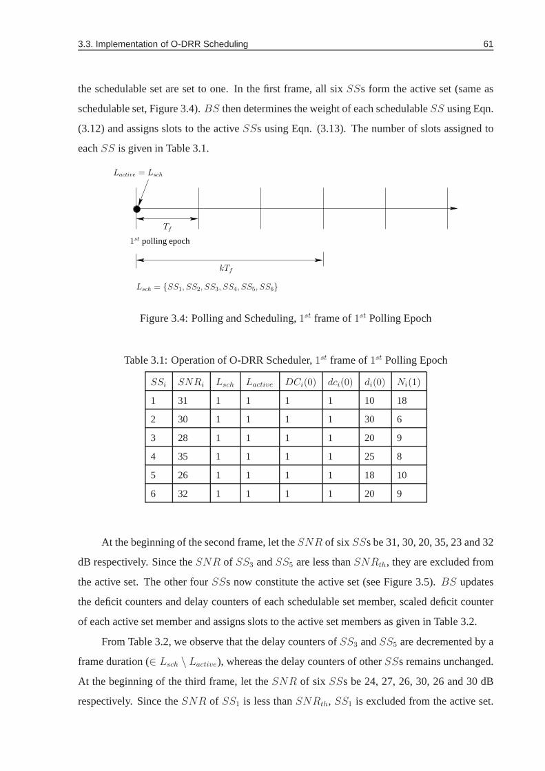
3.3. Implementation of O-DRR Scheduling 61
the schedulable set are set to one. In the first frame, all sixSSs form the active set (same as
schedulable set, Figure 3.4).BS then determines the weight of each schedulableSS using Eqn.
(3.12) and assigns slots to the activeSSs using Eqn. (3.13). The number of slots assigned to
eachSS is given in Table 3.1.
kTf
Tf
Lactive = Lsch
Lsch = {SS1, SS2, SS3, SS4, SS5, SS6}
1st polling epoch
Figure 3.4: Polling and Scheduling,1st frame of1st Polling Epoch
Table 3.1: Operation of O-DRR Scheduler,1st frame of1st Polling Epoch
SSi SNRi Lsch Lactive DCi(0) dci(0) di(0) Ni(1)
1 31 1 1 1 1 10 18
2 30 1 1 1 1 30 6
3 28 1 1 1 1 20 9
4 35 1 1 1 1 25 8
5 26 1 1 1 1 18 10
6 32 1 1 1 1 20 9
At the beginning of the second frame, let theSNR of sixSSs be 31, 30, 20, 35, 23 and 32
dB respectively. Since theSNR of SS3 andSS5 are less thanSNRth, they are excluded from
the active set. The other fourSSs now constitute the active set (see Figure 3.5).BS updates
the deficit counters and delay counters of each schedulable set member, scaled deficit counter
of each active set member and assigns slots to the active set members as given in Table 3.2.
From Table 3.2, we observe that the delay counters ofSS3 andSS5 are decremented by a
frame duration (∈ Lsch \ Lactive), whereas the delay counters of otherSSs remains unchanged.
At the beginning of the third frame, let theSNR of six SSs be 24, 27, 26, 30, 26 and 30 dB
respectively. Since theSNR of SS1 is less thanSNRth, SS1 is excluded from the active set.

62 Chapter 3. Deadline based Fair Uplink Scheduling
kTf
Lactive = {SS1, SS2, SS4, SS6}
Tf
Lsch = {SS1, SS2, SS3, SS4, SS5, SS6}
1st polling epoch
Figure 3.5: Polling and Scheduling,2nd frame of1st Polling Epoch
Table 3.2: Operation of O-DRR Scheduler,2nd frame of1st Polling Epoch
SSi SNRi Lsch Lactive DCi(1) dci(1) di(1) Ni(2)
1 31 1 1 -7 0 10 0
2 30 1 1 5 12 30 20
3 20 1 0 2 NA 20 0
4 35 1 1 3 10 25 19
5 23 1 0 1 NA 18 0
6 32 1 1 2 9 20 21
The other fiveSSs now constitute the active set. TheBS then determines the deficit counter
and delay counter for each schedulableSS, scaled deficit counter for each activeSS. TheBS
then determines the weights of each schedulableSS using Eqn. (3.12) and assigns slots to the
activeSSs using Eqn. (3.13).
From Table 3.3, we observe that the delay counter ofSS1 is decremented by a frame
duration, whereas the delay counters of all otherSSs remain constant. Since we have chosen
k = 3, theBS polls again after the end of the third frame (second polling epoch) to gather the
deadline information of the HoL packet of the connected set.Let theSNR of sixSSs be 30, 24,
26, 28, 31 and 23 dB respectively. Since theSNR of SS2 andSS6 are less thanSNRth, they
will not be polled successfully. Instead,SS1, SS3, SS4 andSS5 are polled successfully and
constitute the schedulable set for the second polling epoch(Figure 3.7). In this polling epoch
M = 4, therefore the quantum sizeQ = 15. At the beginning of the second polling epoch, the
BS resets the deficit counters and the scaled deficit counters ofthe members of the schedulable
set to one. Let at the beginning of second polling epoch, the deadlines associated with the HoL

3.4. Experimental Evaluation of O-DRR Scheduling 63
Lactive = {SS2, SS3, SS4, SS5, SS6}
kTf
Tf
Lsch = {SS1, SS2, SS3, SS4, SS5, SS6}
1st polling epoch
Figure 3.6: Polling and Scheduling,3rd frame of1st Polling Epoch
Table 3.3: Operation of O-DRR Scheduler,3rd frame of1st Polling Epoch
SSi SNRi Lsch Lactive DCi(2) dci(2) di(2) Ni(3)
1 24 1 0 3 NA 10 0
2 27 1 1 -5 4 30 3
3 26 1 1 12 21 15 26
4 30 1 1 -6 3 25 2
5 26 1 1 11 20 13 29
6 30 1 1 -9 0 20 0
packets of sixSSs be 5, 30, 20, 25, 15 and 20 msec respectively. Note thatSS2 andSS6 will
not be considered for scheduling in the second poling epoch.In this example, sinceTH(2) and
TH(6) are greater than one polling epoch (kTf = 15 msec), HoL packets ofSS2 andSS6 will
not be dropped before the next polling epoch.
TheBS then determines the weights of each schedulableSS using Eqn. (3.12) and assigns
slots to the activeSSs using Eqn. (3.13). It updates the deficit counters and the delay counters
for each schedulableSS and the scaled deficit counter for each activeSS in the next frame.
This process continues in every frame of each polling epochs.
3.4 Experimental Evaluation of O-DRR SchedulingIn this section, we describe simulation experiments that have been performed to evaluate O-
DRR scheduling. All the simulations have been conducted using implementations of O-DRR
scheduling in IEEE 802.16 setting in MATLAB [68]. We consider a multipoint-to-point IEEE
802.16 network where 100SSs are connected to a centralizedBS as shown in Figure 3.1.
We further consider WirelessMAN-SC air interface as an example, and use QPSK modulation

64 Chapter 3. Deadline based Fair Uplink Scheduling
Lactive = Lsch
kTf
Tf
Lsch = {SS1, SS3, SS4, SS5}
kTf
1st polling epoch 2nd polling epoch
Figure 3.7: Polling and Scheduling,1st frame of2nd Polling Epoch
Table 3.4: Operation of O-DRR Scheduler,1st frame of2nd Polling Epoch
SSi SNRi Lsch Lactive DCi(0) dci(0) di(0) Ni(1)
1 30 1 1 1 1 5 34
2 24 0 0 NA NA NA NA
3 26 1 1 1 1 20 8
4 28 1 1 1 1 25 7
5 31 1 1 1 1 15 11
6 23 0 0 NA NA NA NA
scheme (mandatory as per the standard) betweenSSs and theBS. We consider two different
sets of experiments. In the first experiment, the deadlinesTds of all flows are the same with
Td = 200 msec. We term this experiment as “single-class” (SC) experiment. In the second
experiment,SSs are divided evenly into two-classes based on their deadline requirements,Td(1)
= 200 msec andTd(2) = 500 msec. We term this experiment as “multi-class” (MC) experiment.
EachSS is assumed to have a large enough buffer such that packets getdropped at aSS only
due to deadline violation. The frame durationTf is set to 1 msec, withNs = 100 slots.
The path loss exponent due to distance is set asγ = 4. We simulate both shadowing as
well as fast fading in our experiments. We also consider Additive White Gaussian (AWGN)
with Power Spectral Density (PSD)N0 = 0.35 (4.5 dB/Hz). The shadowing is modeled as Log-
normal with mean zero and standard deviation (σ) of 8 dB. In each simulation run, the channel
gain due to Log-normal shadowing is kept fixed for a duration of 50 frames. For fast fading,
we consider Rayleigh fading model. The channel gain due to fast fading is modeled as complex
Gaussian random variable or equivalently the power gain is an exponential random variable

3.4. Experimental Evaluation of O-DRR Scheduling 65
with meanβ. The coherence time of Rayleigh fading is considered to be equal to one frame
duration, i.e, the channel gain due to fast fading changes from frame to frame. The value of
β and transmission power is chosen such that the expectedSNR received5 due to Log-normal
shadowing, Rayleigh fading and path loss for aSS at the cell edge is more thanSNRth required
for transmission. We considerSNRth = 12.18 dB, the minimumSNR required for IEEE
802.16-2004 WirelessMAN-SC air interface in our simulations. We also repeat the experiments
with different Log-normal shadowing withσ of 4, 6, 8, 10 and 12 dB.
We model both video traffic [69] and general web traffic [50,70]. To generate video traffic
[69] we use self-similar traffic model based on the random midpoint displacement algorithm
[71]. The self-similar video traffic is generated as fractional Brownian noise (fBn) with Hurst
parameterH = 0.8, mean rate to peak rate ratioρ = 0.3 around the unity link capacity. We
consider fixed packet lengths of 100 bits.
For web-traffic, we generate variable sized packets drawn from a truncated Pareto distri-
bution [50, 70]. This distribution is characterized by three parameters: shape factorξ, modeυ
and cutoff thresholdϕth. The probability that a packet has a sizeℓ can be expressed as:
fTP (ℓ) =ξ · υξ
ℓξ+1, υ ≤ ℓ < ϕth
fTP (ℓ) = η, ℓ ≥ ϕth, (3.15)
whereη can be calculated as:
η =
(ξ
varphith
)ξ
, ξ > 1. (3.16)
We choose shape factorξ = 1.2, modeυ = 50 bits, cutoff thresholdϕth = 500 bits which
provides us an average packet size of 110 bits. In each frame,we generate the arrivals for all
the users using Poisson distribution. Arrivals are generated in an independent and identically
distributed (i.i.d.) manner across the frames. We also use amix traffic case in which approx-
imately 50% of theSSs generate Video traffic and the remaining 50% generate Pareto traffic.
The mean rate of the traffic source is scaled relative to the achievable data rateR to achieve
effective link utilization. We term this as the load of the system.
We determine the optimal polling epoch for both “single-class” and “multi-class” exper-
iments. We use the smallerk which corresponds toTd(1) in both single-class and multi-class
5The expected signal power received at a distanced can be determined as:Pr = Ptd−γβe( (log 10σ)2
200 ). For
details refer to Section 2.1.

66 Chapter 3. Deadline based Fair Uplink Scheduling
experiments. WithR = 40 Mbps,N = 100,α = 0.5,Td = 200 msec andTf = 1 msec, we de-
termine different values ofk with different costc. We evaluate the effect of choosing different
polling epoch on packet drops and fairness.
Each simulation has been performed for a heavy network load to stress test the perfor-
mance of the O-DRR scheduler over a period of 2500 frames (250,000 slots). We also vary the
load from 70% to 95% to evaluate the performance of O-DRR scheduler at different load condi-
tions. The value of each parameter observed has been averaged over 50 independent simulation
runs, with the “warm up” frames (approximately 500 frames) being discarded in each run, to
ensure that the values observed are steady-state values. The simulation parameters are provided
in Table 3.5.
Table 3.5: Summary of Simulation Parameters in O-DRR Scheduling
Simulation Parameter Value
Modulation Scheme QPSK
Frame Duration (Tf ) 1 msec
Number ofSSs 100
Number of Frames 2500
Number of Uplink Slots per Frame (Ns) 100
H 0.8
ρ 0.3
ξ 1.2
υ 50 bits
ϕth 500 bits
Td(1) 200 msec
Td(2) 500 msec
Load 70, 75, 80, 85, 90, 95%
σ (Log-normal shadowing) 4, 6, 8, 10, 12 dB
Poling Interval (k) 10-120
3.4.1 Simulation Results
In this section, we analyze the performance of O-DRR scheduler in terms of percentage of
packets dropped and fairness. To measure fairness, we use Jain’s Fairness Index [65].

3.4. Experimental Evaluation of O-DRR Scheduling 67
Effect of Polling Epochk on Packet Drops
We simulate withk varying from 10 to 120 to assess the performance of O-DRR scheduler
at different polling epochs for both Video and Pareto traffic. In Figures 3.8 - 3.9, we plot the
percentage of packet drops with varying polling epochk for different values of load. From
these figures, we observe a concave relationship between percentage of packets dropped and
k. The high percentage of packets dropped at smallk is due to the large overheads of polling
while at highk, the packet drop is due to the deadline expiry. From these figures, we observe
that at a relatively higher load (90, 95 and 99%) the percentage of packets dropped reaches its
minimum atk = 50 for both Video and Pareto traffic. Therefore, we usek = 50 for the rest of
the simulations.
10 20 30 40 50 60 70 80 90 100 110 1200
2
4
6
8
10
Polling Epoch
Pac
ket D
rop
(%)
Packet Drop vs. Polling Epoch (Video Traffic, σ = 8 dB)
Load=70%Load=75%Load=80%Load=85%Load=90%Load=95%Load=99%
Figure 3.8: Percentage of Packets Dropped at Different Polling Epochs (Video)
Fairness of O-DRR Scheduler
To assess the fairness of the O-DRR algorithm, we determine the Jain’s Fairness Index (JFI)
for both “single-class” and “multi-class” experiments. InFigures 3.10 and 3.11, we plot JFI
of O-DRR scheduler at different loads, keeping the Log-normal shadowing parameter constant
(σ = 8 dB). From these figures, we observe that JFI is above 98% for all traffic cases (Video,
Pareto and Mixed). We also observe that JFI decreases with increase in load.

68 Chapter 3. Deadline based Fair Uplink Scheduling
10 20 30 40 50 60 70 80 90 100 110 1200
2
4
6
8
10
Polling Epoch
Pac
ket D
rop
(%)
Packet Drop vs. Polling Epoch (Pareto Traffic, σ = 8 dB)
Load=70%Load=75%Load=80%Load=85%Load=90%Load=95%Load=99%
Figure 3.9: Percentage of Packets Dropped at Different Polling Epochs (Pareto)
70 75 80 85 90 950.9
0.92
0.94
0.96
0.98
1
Load (%)
Jain
’s F
airn
ess
Inde
x
JFI vs. Load: Single−Class Traffic (k = 50, σ = 8 dB)
O−DRR(Video)−SCO−DRR(Pareto)−SCO−DRR(Mix)−SC
Figure 3.10: Jain’s Fairness Index at Different Loads: Single-Class Traffic

3.4. Experimental Evaluation of O-DRR Scheduling 69
70 75 80 85 90 950.9
0.92
0.94
0.96
0.98
1
Load (%)
Jain
’s F
airn
ess
Inde
xJFI vs. Load: Multi−Class Traffic (k = 50, σ = 8 dB)
O−DRR(Video)−MCO−DRR(Pareto)−MCO−DRR(Mix)−MC
Figure 3.11: Jain’s Fairness Index at Different Loads: Multi-Class Traffic
4 6 8 10 120.9
0.92
0.94
0.96
0.98
1
Log−normal Shadowing (σ) in dB
Jain
’s F
airn
ess
Inde
x
JFI vs. Sigma: Single−Class Traffic (load = 95%, k = 50)
O−DRR(Video)−SCO−DRR(Pareto)−SCO−DRR(Mix)−SC
Figure 3.12: Jain’s Fairness Index at Different Log-normalShadowing: Single-Class Traffic

70 Chapter 3. Deadline based Fair Uplink Scheduling
4 6 8 10 120.9
0.92
0.94
0.96
0.98
1
Log−normal Shadowing (σ) in dB
Jain
’s F
airn
ess
Inde
xJFI vs. Sigma: Multi−Class Traffic (load = 95%, k = 50)
O−DRR(Video)−MCO−DRR(Pareto)−MCO−DRR(Mix)−MC
Figure 3.13: Jain’s Fairness Index at Different Log-normalShadowing: Multi-Class Traffic
In Figures 3.12 and 3.13, we plot JFI of O-DRR scheduler for different values of Log-
normal shadowing,σ = 4, 6, 8, 10 and12 dB, with the load being fixed at 95%. From these
figures, we observe that JFI is above 98% for all traffic cases.From Figures 3.10 - 3.13, we
observe that JFI is above 98% even at 95% load for all values ofσ.
3.4.2 Comparison with Round Robin Scheduler
We compare the performance of O-DRR scheduler with a simple Round Robin (RR) scheduler.
Like the O-DRR scheduler, we also use the polling method to determine the schedulable list
at the beginning of the polling epoch for the RR scheduler. The polling epochk used in RR
scheduler is same as that used in O-DRR scheduler. Unlike O-DRR scheduler, however, in RR
scheduler, theBS schedules the activeSSs in every frame in a simple round robin manner.
In this section, we compare the percentage of packets dropped and JFI of O-DRR scheduler
with that of RR scheduler at: (a) Different Loads; (b) Different Log-normal Shadowing; and (c)
Different Polling Epochs.
For Varying Values of Load
In Figures 3.14, 3.15 and 3.16, we plot the percentage of packets dropped observed in both RR
and O-DRR scheduler at different loads for Video, Pareto andMixed traffic respectively. The

3.4. Experimental Evaluation of O-DRR Scheduling 71
70 75 80 85 90 950
1
2
3
4
5
6
Load (%)
Pac
ket D
rop
(%)
Packet Drop vs. Load (k = 50, σ = 8 dB)
RR(Video)O−DRR(Video)
Figure 3.14: Percentage of Packets Dropped at Different Loads with Multi-Class Video Traffic
value ofk andσ are kept constant (k = 50 andσ = 8 dB) in these figures. From these figures,
we observe that the O-DRR scheduler out-performs RR scheduler in packet drop percentage
for all traffic cases. Since O-DRR is a deadline based scheduler, flows with relatively smaller
deadlines are scheduled with higher priority than the flows with higher deadlines. This improves
the performance of the scheduler and minimizes packet dropsdue to deadline violation, which is
reflected in these figures. In Figure 3.17, we plot the percentage gain (improvement) in packets
dropped of O-DRR scheduler over that of RR scheduler at different loads. From this figure,
we observe that the O-DRR scheduler performs better at relatively high loads as compared to
relatively low loads. We also observe that when the load is 95%, the improvements of O-DRR
scheduler over RR scheduler are around 37%, 27% and 18% for Video, Mixed and Pareto traffic
respectively. The high relative improvement of packet droppercentage of O-DRR scheduler
over RR scheduler signifies the superiority of O-DRR scheduler over RR scheduler in an IEEE
802.16 network.
Moreover, from Figures 3.18, 3.19 and 3.20, we observe that JFI achieved by O-DRR
scheduler is more than that of RR scheduler. This signifies the fairness properties of O-DRR
scheduler as compared to RR scheduler at different loads.

72 Chapter 3. Deadline based Fair Uplink Scheduling
70 75 80 85 90 950
1
2
3
4
Load (%)
Pac
ket D
rop
(%)
Packet Drop vs. Load (k = 50, σ = 8 dB)
RR(Pareto)O−DRR(Pareto)
Figure 3.15: Percentage of Packets Dropped at Different Loads with Multi-Class Pareto Traffic
70 75 80 85 90 950
1
2
3
4
5
6
Load (%)
Pac
ket D
rop
(%)
Packet Drop vs. Load (k = 50, σ = 8 dB)
RR(Mix)O−DRR(Mix)
Figure 3.16: Percentage of Packets Dropped at Different Loads with Multi-Class Mixed Traffic

3.4. Experimental Evaluation of O-DRR Scheduling 73
70 75 80 85 90 950
10
20
30
40
50
Load (%)
Red
uctio
n (%
)
Reduction in Packet Drop vs. Load (k = 50, σ = 8 dB)
VideoParetoMix
Figure 3.17: Performance Gain of O-DRR Scheduler over RR Scheduler in terms of PacketDrops at Different Loads
70 75 80 85 90 950.9
0.92
0.94
0.96
0.98
1
Load (%)
Jain
’s F
airn
ess
Inde
x
JFI vs. Load (k = 50, σ = 8 dB)
RR(Video)O−DRR(Video)
Figure 3.18: Jain’s Fairness Index at Different Loads with Multi-Class Video Traffic

74 Chapter 3. Deadline based Fair Uplink Scheduling
70 75 80 85 90 950.9
0.92
0.94
0.96
0.98
1
Load (%)
Jain
’s F
airn
ess
Inde
x
JFI vs. Load (k = 50, σ = 8 dB)
RR(Pareto)O−DRR(Pareto)
Figure 3.19: Jain’s Fairness Index at Different Loads with Multi-Class Pareto Traffic
70 75 80 85 90 950.9
0.92
0.94
0.96
0.98
1
Load (%)
Jain
’s F
airn
ess
Inde
x
JFI vs. Load (k = 50, σ = 8 dB)
RR(Mix)O−DRR(Mix)
Figure 3.20: Jain’s Fairness Index at Different Loads with Multi-Class Mixed Traffic

3.4. Experimental Evaluation of O-DRR Scheduling 75
For Varying Values of Standard Deviation (σ) of Log-Normal Shadowing
We also vary theσ of Log-normal shadowing from 4 dB to 12 dB to determine the robustness
of the O-DRR scheduler compared to that of RR scheduler. In Figures 3.21 and 3.22, we plot
the percentage of packets dropped observed for Video and Pareto traffic respectively in both
RR and O-DRR scheduler at different values of Log-normal shadowing. The values ofk and
load are kept constant (k = 50, load = 95%) in these figures. From these figures, we observe
that the O-DRR scheduler out-performs RR scheduler in packet drop percentage for both traffic
cases. In Figure 3.23, we plot the percentage gain (improvement) in packets dropped of O-DRR
scheduler over RR scheduler for different values ofσ of Log-normal shadowing. From this
figure, we observe that the O-DRR scheduler performs better than the RR scheduler even when
the Log-normal shadowing is high. We also observe that at 95%load and atσ = 12 dB, the
improvements of O-DRR scheduler over RR scheduler are more than 40% for both Video and
Pareto traffic. Therefore, O-DRR scheduler is more suitablefor all load, all fading and traffic
requirements.
4 6 8 10 120
1
2
3
4
5
6
Log−normal Shadowing (σ) in dB
Pac
ket D
rop
(%)
Packet Drop vs. σ (k = 50, load = 95%)
RR(Video)O−DRR(Video)
Figure 3.21: Percentage of Packets Dropped at Different Log-normal Shadowing with Multi-Class Video Traffic

76 Chapter 3. Deadline based Fair Uplink Scheduling
4 6 8 10 120
1
2
3
4
5
6
Log−normal Shadowing (σ) in dB
Pac
ket D
rop
(%)
Packet Drop vs. σ (k = 50, load = 95%)
RR(Pareto)O−DRR(Pareto)
Figure 3.22: Percentage of Packets Dropped at Different Log-normal Shadowing with Multi-Class Pareto Traffic
4 6 8 10 120
10
20
30
40
50
Log−normal Shadowing (σ) in dB
Red
uctio
n (%
)
Reduction in Packet Drop vs. σ (k = 50, load = 95%)
VideoPareto
Figure 3.23: Performance Gain of O-DRR Scheduler over RR Scheduler in terms of PacketDrops at Different Log-normal Shadowing

3.4. Experimental Evaluation of O-DRR Scheduling 77
Moreover, from Figures 3.24 and 3.25, we observe that JFI achieved by O-DRR scheduler
is more than that of RR scheduler. This signifies the fairnessproperties of O-DRR scheduler as
compared to that of RR scheduler for different values ofσ of Log-normal shadowing.
4 6 8 10 120.9
0.92
0.94
0.96
0.98
1
Log−normal Shadowing (σ) in dB
Jain
’s F
airn
ess
Inde
x
JFI vs. σ (k = 50, load = 95%)
RR(Video)O−DRR(Video)
Figure 3.24: Jain’s Fairness Index at Different Log-normalShadowing with Multi-Class VideoTraffic
4 6 8 10 120.9
0.92
0.94
0.96
0.98
1
Log−normal Shadowing (σ) in dB
Jain
’s F
airn
ess
Inde
x
JFI vs. σ (k = 50, load = 95%)
RR(Pareto)O−DRR(Pareto)
Figure 3.25: Jain’s Fairness Index at Different Log-normalShadowing with Multi-Class ParetoTraffic

78 Chapter 3. Deadline based Fair Uplink Scheduling
For Varying Values of Polling Epochk
We also compare JFI achieved by O-DRR with that of RR at different values ofk, keeping
σ = 8 dB and load = 95% as fixed. The results are plotted in Figures 3.26 and 3.27. We observe
that JFI achieved by O-DRR is more than that of RR at differentpolling epochs.
10 20 30 40 50 60 70 80 90 100 110 1200.9
0.92
0.94
0.96
0.98
1
Polling Epoch
Jain
’s F
airn
ess
Inde
x
JFI vs. Polling Epoch (load = 95%, σ = 8 dB)
RR(Video)O−DRR(Video)
Figure 3.26: Jain’s Fairness Index at Different Polling Epochs with Multi-Class Video Traffic
10 20 30 40 50 60 70 80 90 100 110 1200.9
0.92
0.94
0.96
0.98
1
Polling Epoch
Jain
’s F
airn
ess
Inde
x
JFI vs. Polling Epoch (load = 95%, σ = 8 dB)
RR(Pareto)O−DRR(Pareto)
Figure 3.27: Jain’s Fairness Index at Different Polling Epochs with Multi-Class Pareto Traffic

Chapter 4
TCP-aware Fair Uplink Scheduling -
Fixed Modulation
In the previous chapter, we have considered scheduling of real-time applications. Real-time
applications require QoS guarantees in terms of minimum bandwidth and maximum latency
from the network. Typically these applications employ UDP as the transport layer protocol.
Non real-time Internet applications employ TCP as the transport layer protocol. We term these
applications as TCP-based applications. Unlike real-timeapplications, the TCP-based applica-
tions do not operate within the strict guarantee QoS framework. Instead, a TCP source adapts
its rate of transmission based on the feedback received fromthe sink. However, if the under-
lying scheduling mechanism does not consider this rate adaptation, then it may assign more or
less bandwidth than the flows’ requirement. If it assigns more bandwidth than required, then
bandwidth idleness results. This may lead to aggregate TCP throughput degradation. Similarly,
if it assigns less bandwidth than required, then the TCP source will not be able to transmit at its
rate resulting in degradation in throughput. This suggeststhat the scheduler should assign band-
width based on the requirement of the TCP flows. Since Round Trip Time (RTT ) of TCP flows
are different, the rate of adaptation of transmission rate of TCP flows are different. Therefore,
users with smallRTT may grab more bandwidth as compared to users with largeRTT . This
may lead to unfairness. In wireless networks, bandwidth idleness and throughput degradation
become more severe as the channel is time varying in nature. This is because, if the scheduler
assigns bandwidth to a flow whose Signal to Noise Ratio (SNR) is not suitable for transmission,
then bandwidth allocated to that flow will be not be utilized.We therefore, propose fair TCP
79

80 Chapter 4. TCP-aware Fair Uplink Scheduling - Fixed Modulation
Window-aware Uplink Scheduling (TWUS) and Deadline-basedTCP Window-aware Uplink
Scheduling (DTWUS) schemes that are cognizant of TCP rate adaptation and the time varying
nature of wireless channel.
Though the proposed schemes can be employed in any cellular network, we consider the
uplink of multipoint-to-point IEEE 802.16 based WiMAX network in this chapter. As discussed
in Chapter 2, the IEEE 802.16 standard defines four service classes such asUGS, rtPS, nrtPS
andBE. Since TCP-based applications can fall undernrtPSandBEservice classes, the proposed
schedulers can be used to schedulenrtPSandBEservice classes. The standard allows both fixed
and adaptive modulation schemes in the PHY layer. In this chapter, we consider fixed modula-
tion scheme and in the next chapter we consider adaptive modulation scheme. Using exhaustive
simulations, we demonstrate the improvement in TCP throughput achieved by the TCP-aware
schedulers over non TCP-aware schedulers. Along with the throughput improvement, we also
demonstrate fairness capability and robustness of the scheduling schemes at different channel
fading.
In Section 4.1, we explain the characteristics of TCP and theimpact of scheduling on
TCP performance. In Section 4.2, we discuss the system modeland the motivation behind the
TCP-aware uplink scheduling schemes. In Section 4.3, we present both TCP Window-aware
Uplink Scheduling and Deadline-based TCP Window-aware Uplink Scheduling scheme with
fixed modulation. In Section 4.4, we discuss the experimental set up and present the results.
These results demonstrate the efficiency of the proposed algorithms. We provide the concluding
remarks in Section 4.5.
4.1 Transmission Control Protocol
In this section, we discuss TCP and its characteristics. Though, the contents of this section are
standard, we introduce the terminology that has been used inthe rest of the chapter. A more
comprehensive account of TCP and its characteristics can befound in [42,43,72].
TCP is a connection oriented protocol which uses a three-wayhandshaking mechanism
to establish a connection between a source and a sink or destination. It allows the source to
transmit back to back packets limited by the congestion window (cwnd) size. For every packet
the source transmits, it sets a timeout (which known as TCP timeout) before which the source
should get an acknowledgement (ACK) for that packet from the sink. The sink transmitsACK

4.1. Transmission Control Protocol 81
packets for successful reception of either every packet or agroup of packets. On successful
reception of theACKs, the source increases itscwnd size and transmits further packets to the
sink. However, the data as well as theACK packets can be lost in the network. To detect the
loss of packets, TCP uses two different mechanisms. In the first mechanism, the source assumes
packet loss if it receives three duplicateACKs (dupacks) of a single packet in succession. In
the second mechanism, the source assumes packet loss if the source does not receive anyACK
before the expiry ofTCP timeout. On detecting a packet loss, the source decreases itscwnd size
and retransmits the un-acknowledged packets again. The change incwnd size from its current
value occurs after a minimum duration called Round Trip Time(RTT ). In most of the TCP
implementations, the value ofRTT is estimated by the source using exponential averaging as
follows:RTTestimated = Υ ×RTTestimated + (1 − Υ) × RTTmeasured, (4.1)
whereΥ is a constant (0 < Υ < 1).In TCP, instead of using linear increase and decrease ofcwnd, Additive Increase and
Multiplicative Decrease (AIMD) method is employed. Moreover, the manner of increase and
decrease ofcwnd size is different for different TCP implementations. In most of the TCP
implementations, such as TCP Reno and NewReno [73, 74],cwnd drops to one, if the source
does not receive anACK before the TCP timeout. Further, it drops itscwnd to half of its
current size, if it receives threedupacksin succession.
The increase ofcwnd size occurs in two phases. In the first phase,cwnd increases in
an exponential manner. This phase is also called asslow startphase. In this phase, for every
successfulACK that the source receives, TCP increases itscwnd size multiplicatively by a
factor of two until it reaches a threshold known asssthresh. After it reachesssthresh, it enters
the second phase. In this phase, it increases itscwnd size by one for every successfulACK
received by it. The increase ofcwnd size continues until the source receives threedupacksor
experiences TCP timeout or it reaches its maximum valuecwndMax. Once it reachescwndMax,
it continues transmitting with this window size till it experiences congestion (either it receives
triple dupacksor experiences TCP timeout). If it receives threedupacks, then it updatesssthresh
with its new valuecwnd2
and enters the linear increase phase. If it experiences TCP timeout,
then it drops itscwnd size to one and enters the exponential increase phase again.This process
continues till the connection lasts. Thecwnd evolution of TCP Reno [73] is depicted in Figure
4.1.

82 Chapter 4. TCP-aware Fair Uplink Scheduling - Fixed Modulation
Time (RTT )RTT
ssthresh
New ssthresh
Trippledupacks Received
TCP timeout OccursExp
onen
tial I
ncre
ase
Linear Increase
cwnd
size
inP
acke
ts
Figure 4.1: Congestion Window Evolution of TCP Reno
As discussed earlier, the actual rate of transmission of TCP-based applications is con-
trolled by thecwnd size. Hence,cwnd size has a significant impact on TCP performance. In
the next section, we discuss impact of scheduling on TCP performance.
4.1.1 Impact of Scheduling on TCP Performance
In this section, we discuss the impact of underlying scheduling mechanism on TCP perfor-
mance. The impact of scheduling on TCP performance can have two major aspects, such as (i)
TCP throughput and (ii) fairness. If the scheduling scheme assigns slots without considering the
cwnd size of the TCP flows, then the flows withcwnd = 1 as well as withcwnd = cwndMax
will be assigned with equal number of slots. For a flow withcwnd = 1, slots will be underuti-
lized as its requirement is small, whereas for a flow withcwnd = cwndMax, the number of slots
assigned to it may not be adequate to meet its requirement. This results in increase in schedul-
ing delay and may lead to TCP timeouts. Therefore, if the scheduling scheme does not consider
thecwnd size of the TCP flows, then TCP throughput suffers and slots get under-utilized,
Like throughput, fairness is also an important parameter ofa scheduler. As discussed
before, TCP flows with smallRTTs increase theircwnd size at a faster rate as compared to the
TCP flows with largeRTTs. Hence, if the scheduler assigns slots only based oncwnd sizes,
then the flows with smallRTTs will acquire more number of slots as compared to the flows
with relatively largeRTTs. Therefore, if the scheduling scheme does not considerRTTs of

4.2. System Model 83
SS1
SS2
SSN
BS
cwnd1
cwnd2
cwndN
F low2
F low
N
F low1
TCP Traffic Sources
TC
PS
inks
Figure 4.2: Multipoint-to-Point Framework with TCP-basedApplications
the TCP flows, it may result in unfairness among the flows.
4.2 System Model
We consider a multipoint-to-point network where multipleSSs are connected to oneBS as
shown in Figure 4.2. This scenario may correspond to a singlecell IEEE 802.16 [3] system.
Though some part of this model are similar to that discussed in the previous chapter, we re-state
the important assumptions required for this chapter.
BS is the centralized entity responsible for scheduling the TCP flows. We assume that
theSSs are TCP traffic sources. Each packet is associated with a TCPflow (also known as
source-sink pairs) and each flow is associated with aSS. Though this can be generalized to
multiple flows perSS, we consider a single flow perSS. TCP acknowledgement (ACK)
packets traverse from the sink to the source in the downlink direction. We further assume that
theACK packets are very small and the downlink scheduler at theBS schedules theseACK
packets without any delay.
Time is divided into frames. Each frame (of duration ofTf ) in turn is composed of a fixed
number of slots of equal duration ofTs. We assume time varying wireless channel between a
SS and theBS. We assume that the channel gains betweenSSs and theBS are independent
and identically distributed (i.i.d.). We further assume that the coherence time of the channel is
84 Chapter 4. TCP-aware Fair Uplink Scheduling - Fixed Modulation
greater than the frame duration, i.e., the channel state remains constant during a frame duration.
The channel state changes from frame to frame according to Rayleigh fading model. We also
consider Log-normal shadowing and path loss in modelling the channel gain. We assume that
the individual channel state information is available at the BS in every frame. LetSNRi
denote theSNR measured betweenSSi and theBS. Packets can be successfully received if
SNRi ≥ SNRth. The value ofSNRth depends upon the modulation and coding scheme used
at the Physical (PHY) layer. Since we consider fixed modulation technique in this chapter, the
maximum attainable data rate is also fixed.
We assume that a setI of TCP flows shares a network ofI unidirectional links through
theBS1. The capacity of the individual linki denoted byci, for i = 1, 2, 3, ...I, is a function of
theSNR of the corresponding link.ci can also be considered as maximum attainable data rate
at link i. Since the channel state varies from frame to frame,ci also varies from frame to frame.
4.2.1 Motivation and Problem Formulation
In this section, we motivate for a centralized polling baseduplink scheduling algorithm for
TCP-based applications. As pointed out in Chapters 1 and 2, traditional scheduling schemes
like Weighted Fair Queuing (WFQ) [26], Self-Clocked Fair Queueing (SCFQ) [27] and Worst-
case Fair Weighted Fair Queuing (WF2Q) [28], etc., cannot be used for the uplink scheduling.
Instead, variants of Round Robin (RR) schedulers are the candidates for uplink scheduling.
Since the channel state ofSSs varies randomly across the frames, a RR scheduler would result
in unfairness. Moreover, RR scheduler does not considercwnd size,RTT and TCP timeout
while scheduling. As discussed in Section 4.1.1, since TCP throughput as well as fairness suf-
fers if the underlying scheduling scheme does not considercwnd size andRTT of the flows, a
simple RR scheduler is not appropriate. Therefore, we propose TCP-aware scheduling mech-
anisms, which attempt to schedule flows based oncwnd size and TCP timeouts as well as
maintain fairness among the flows.
For the centralized uplink scheduling, theSSs are required to communicate their band-
width requirements with theBS either in a contention mode or in a polling mode. Sincecwnd
size of aSS does not change for oneRTT , the rate of transmissionx = cwndRTT
remains constant
for oneRTT . Hence, bandwidth requirement of anySS does not change for oneRTT . In prac-
1We assume one to one mapping between the flows and the links.

4.3. TCP-aware Uplink Scheduling with Fixed Modulation 85
tice, oneRTT spans over 150 to 200 msec, whereas one frame duration is of the order of 1 to 5
msec. Hence, contention based scheduling, where bandwidthrequest is communicated in every
frame, is not appropriate. Instead, a polling based solution, where bandwidth requirement is
communicated after certain number of frames (called polling epoch) is more appropriate. Since
the resource requirement changes only after oneRTT , selecting a polling epoch of duration
less than oneRTT is not appropriate.
Unlike wired network, the time varying nature of wireless channel and the modulation
techniques used at the PHY layer also have an impact on scheduling. As discussed before,
we consider fixed modulation in this chapter. In addition, weexploit the idea of Opportunistic
scheduling while designing these systems. Since we use bothcwnd size and TCP timeout
in the scheduling process, we classify the scheduling schemes into (i) TCP Window-aware
Uplink Scheduling (TWUS) with Fixed Modulation; and (ii) Deadline-based TCP Window-
aware Uplink Scheduling (DTWUS) with Fixed Modulation. We discuss the details of the
scheduling algorithms in the subsequent sections.
4.3 TCP-aware Uplink Scheduling with Fixed Modulation
Before discussing the scheduling algorithm, we define the following terms. Though the terms
defined here are similar to the terms defined in the previous chapter, we re-state them in the
context of TCP-aware scheduling.
• Connected Set: The set ofSSs that has been admitted into the system through an admis-
sion control and connection set up phase is called connectedset (Lconnect). LetN be the
cardinality of the connected set.
• Polling Epoch: It is defined as the interval that theBS chooses to poll the connectedSSs.
In the proposed scheduling algorithm, the polling is performed by theBS only once after
everyk frame.
• Schedulable Set: A SS is schedulable, if at the beginning of a polling epoch, it hasa non
zerocwnd size and theSNR of its wireless link to theBS is above a minimum threshold
SNRth. The set of suchSSs constitute a schedulable setLsch. This set may change
dynamically across the polling epochs. LetM be the cardinality of the schedulable set.

86 Chapter 4. TCP-aware Fair Uplink Scheduling - Fixed Modulation
• Active Set: An activeSS is defined to be one that is schedulable during a given frame of
a polling epoch and was schedulable at the beginning of that epoch. The set of suchSS
constitutes an active setLactive. During a polling epoch, theBS only schedules traffic
from the active set. The membership of an active set may change dynamically across
the frames, whereas the membership of a schedulable set may change across the polling
epochs.
• Quantum Size: It is the number of slots that should be assigned to any of theschedulable
SS in any frame of a polling epoch. At the beginning of every polling epoch, theBS
determines the quantum size as:Q = Ns
M, whereNs is the total number of uplink slots
available for scheduling. SinceM is fixed for a polling epoch,Q is also fixed for a polling
epoch.
We divide the proposed scheduling algorithm into two phases: pollingandslot assignment.
The periodic polling epochk is a function ofRTTs of the contending flows. We discuss the
determination of polling epochk in the next section in detail.BS polls all connectedSSs after
everyk frames. Once the polling is performed, theBS schedules the activeSSs in every frame.
The relationship between polling epoch and frame by frame scheduling is illustrated in Figure
4.3.
Polling EpochPolling Polling
Scheduling
Tf
Frame1 Frame2 Framek
Figure 4.3: Polling and Frame by Frame Scheduling in TCP-aware Scheduling
Let PL denote the length of a packet in bits. The number of slots required to transmit
cwnd number of packets at rateR in bits/sec is expressed as:
nreqi =cwndi × PL
R× Ts. (4.2)
nreqi is the total number of slots required bySSi to transmitcwndi number of packets
in oneRTT duration. However, both the channel gains and the number of slots assigned to

4.3. TCP-aware Uplink Scheduling with Fixed Modulation 87
eachSS are different from frame to frame. Therefore, the amount of data transmitted by each
SS differs from frame to frame. Hence, the determination ofnreqi at the beginning of polling
epoch is not appropriate. Instead, there is a need to determine the number of slots required
using the resource requirement and capacity of the link in every frame. Resource requirement
is determined by the scheduler by determining
Di(0) = cwndi × PL,
Di(n) = cwndi × PL− Txi(n− 1), ∀n ∈ [1, k],(4.3)
whereTxi(n− 1) is the total amount of data (in bits) transmitted bySSi from the beginning of
the current polling epoch to the frame under consideration.At the beginning of a polling epoch,
the amount of data transmitted by aSS is set to zero, i.e.,Txi(0) = 0, ∀i ∈ I. The number of
slots required bySSi in nth frame is given by:
nreqi (n) =Di(n)
R× Ts. (4.4)
At the time of polling, each polledSS needs to communicate itscwnd in terms of the
number of slots required and itsRTT with theBS. In the subsequent sections, we first discuss
the method to chose the polling epoch and then discuss the method of slot assignment by the
BS. Note that, like O-DRR scheduler, TCP-aware schedulers require flow level information
only.
4.3.1 Determination of Polling Epochk
The polling epochk is an important parameter of the proposed scheduler.k should be chosen in
such a manner that the system efficiency and fairness are maintained. We argue that the polling
epochk should be the minimumRTT 2 among all TCP flows going through theBS. This is
because, the TCP timeout value is typically chosen to be fourto five times theRTT in most
TCP implementations. Therefore, if we choose the polling epoch to be equal to twoRTTs, then
anySS with an ongoing TCP flow that misses polling needs to be polledat the next opportunity.
Similarly, if the polling epoch is more than twoRTTs, and if theBS misses oneSS with a
2Typical TCPRTT s are in the range of 100 msec - 200 msec, whereas the frame length Tf in IEEE 802.16 is
0.5 msec, 1 msec or 2 msec.

88 Chapter 4. TCP-aware Fair Uplink Scheduling - Fixed Modulation
TCP flow, then congestion window reduction for that TCP flow islikely to occur with high
probability. This is because, the chances of not getting scheduled at the next opportunity before
TCP timeout is very high. If polling is very frequent, i.e., more than once perRTT , then more
control slots will be utilized for polling. Moreover, frequent polling is not preferable, since the
cwnd size itself changes after oneRTT . Hence, we choose the polling epoch to be equal to the
min{RTT} of the active TCP flows. In the proposed scheduling scheme, after every polling
epoch, theBS determines the next polling epoch based on themin{RTT}received from the
polledSSs of the current polling epoch.
4.3.2 Slot Assignments using TCP Window-aware Uplink Scheduling
BS maintains an indicator variableF lagi for eachSS. F lagi is 1, if SSi is scheduled in a
frame, and 0 otherwise. LetNi(n) be the total number of slots assigned toSSi in framen.
Based on the number of slots assigned in the previous frame and cwnd size, theBS determines
the resource requirement for each schedulableSS in every frame.Di(n) (as defined in Eqn.
(4.3)) of a schedulableSS in framen is updated as:
Di(n) = cwndi × PL− Txi(n− 1)
= Di(n− 1) − F lagi(n− 1) ×Ni(n− 1) ×R × Ts, ∀n ≥ 1,(4.5)
whereR is the rate of transmission betweenSSs and theBS. In this caseR is fixed. At the
beginning of a polling epoch, resource requirement of eachSS is equivalent to the number of
slots required to transmit itscwnd size, i.e.,Di(0) = cwndi×PL. In a polling epoch, ifDi(n)
of SSi becomes zero, thenSSi is withdrawn from the active set.
We utilize DRR’s idea of maintaining a quantum sizeQ for each schedulableSS. The
quantum sizeQ is kept fixed for one polling epoch. The number of slots assigned to any
subscriber stationSSi in framen can be greater or smaller than the quantum size. To keep a
track of the number of slots assigned with respect to the quantum sizeQ, we use a credit-based
approach. The credit-based approach employs one deficit counter for eachSSi similar to DRR.
The idea of a deficit counter is to ensure fairness among the subscriber stations in long term. At
the beginning of a polling epoch, deficit counter ofSSi is initialized to one. The deficit counter
DCi(n) is updated in every frame as:

4.3. TCP-aware Uplink Scheduling with Fixed Modulation 89
DCi(0) =1,
DCi(n) =DCi(n− 1) +Q− F lagi(n− 1) ×Ni(n− 1), ∀i ∈ Lsch, ∀n ≥ 1.(4.6)
From the above equation, we observe that the deficit countersof all schedulableSSs are
incremented by the quantumQ, whereas the deficit counter of all activeSSs are decremented
by the amount of slots received in the previous frame. We define scaled deficit counterdci as
follows:
dci(0) =1, ∀i ∈ Lactive,
dci(n) =DCi(n) + minj
|DCj(n)|, ∀i, j ∈ Lactive, ∀n ≥ 1. (4.7)
At the beginning of a polling epoch, the scaled deficit counter dci of SSi is initialized to
one. After determining the resource requirement and scaleddeficit counter, theBS determines
the weight of each active setSS. For all otherSSs, the weights are zero.BS determines the
weightWi(n) for SSi in framen using the following equation:
Wi(n) =Di(n) × dci(n)
∑
j∈LactiveDj(n) × dcj(n)
, ∀i ∈ Lactive, ∀n ≥ 1. (4.8)
Eqn. (4.8) essentially determines a weightWi(n) for anSSi in framen, which is pro-
portional to the normalized product of the scaled deficit counter and resource requirement (and
hence thecwnd). If a TCP flow has a smallerRTT , its cwnd size will be increased at a faster
rate. Since we chosek = mini{RTTi}, at the beginning of each polling epoch,SS with the
smallestRTT will update itscwnd size, whereas others will not. This will result in increase
in resource requirement of aSS whoseRTT is small as compared to otherSSs. Hence, by
allocating the number of slots in proportion to the resourcerequirement, will result in allocation
of larger share of slots to such flows. This will also result inunfairness among theSSs. The
credit-based approach proposed by us ensures that the scaled deficit counter value is small for
such flows and thereby ensures fairness. After the determination of weights, theBS assigns the
number of slots toSSi in framen using:
Ni(n) =Wi(n) ×Ns
∑
j∈LactiveWj(n)
, ∀i ∈ Lactive, ∀n ≥ 1. (4.9)

90 Chapter 4. TCP-aware Fair Uplink Scheduling - Fixed Modulation
In the next section, we exploit the knowledge of TCP timeout along with the congestion
window size information and propose another scheduling mechanism. We call this scheduling
algorithm as Deadline-based TCP Window-aware Uplink Scheduling (DTWUS).
4.3.3 Slot Allocation using Deadline-based TCP Window-aware Uplink
Scheduling
In this scheme, the determination of deficit counter, scaleddeficit counter and resource require-
ment for eachSS is similar to that defined in TWUS scheduler. However, the method of deter-
mination of weights for scheduling is different from that defined in Eqn. (4.8). In this scheme,
we use TCP timeout information along with resource requirement and deficit counter values to
determine the weights. In this scheme, at the beginning of the polling, each polledSS com-
municates itscwnd size, time left to reach TCP timeout (TTO) (of the last un-acknowledged
packet), TCP timeout andRTT to theBS.
For each schedulableSS, we definedeadlinedi to be a measure of its rate of approach
towards the TCP timeout. At the beginning of a polling epoch,let TTOi denote the maximum
duration that the TCP flow ofSSi can wait before reaching TCP timeout. Note that the maxi-
mum value ofTTOi is the TCP timeout3 associated with the TCP flow belongs toSSi. At the
beginning of a polling epoch,di of SSi is initialized toTTOi. If SSi is scheduled in framen,
then the deadlinedi(n) remains unchanged, i.e, it takes the value ofdi(n−1). Otherwise,di(n)
is decremented by one frame duration from its previous value. BS updates the deadline of the
schedulable flows as follows:
di(0) =TTOi, ∀i ∈ Lconnected,
di(n) =di(n− 1) − Tf , ∀i ∈ (Lsch \ Lactive), ∀n ≥ 1,
di(n) =di(n− 1), ∀i ∈ Lactive, ∀n ≥ 1.
(4.10)
If Tf exceedsdi(n), then the deadlinedi(n) of SSi is initialized to TCP timeout (TOi)
of thatSS. In that case, TCP flow experiences a timeout before getting scheduled, resulting in
reduction ofcwndi to one. After determining the scaled deficit counter as in Eqn. (4.7) and
deadline as in Eqn. (4.10), theBS determines weightWi(n) for SSi in framen using:
3TCP flows generally start at random and hence different flows have different residual times to reach TCP
timeout.

4.4. Experimental Evaluation of TCP-aware Schedulers 91
Wi(n) =
Di(n)×dci(n)di(n)
∑
j∈Lactive
Dj(n)×dcj(n)
dj(n)
, ∀i ∈ Lactive, ∀n ≥ 1. (4.11)
After the determination of weights, the number of slots assigned by theBS to SSi in
framen is determined as:
Ni(n) =Wi(n) ×Ns
∑
j∈LactiveWj(n)
, ∀i ∈ Lactive, ∀n ≥ 1. (4.12)
The use of deadline in weight determination ensures that a higher number of time slots are
assigned to aSS that has a smaller deadline.
The pseudo-code of the proposed schedulers TWUS and DTWUS ispresented in Algo-
rithm 2. We combine both schedulers by usingF lagdeadline, which is set to one for DTWUS and
is set to zero for TWUS. In the next section, we discuss the experimental setup and simulation
results in an IEEE 802.16 setting.
4.4 Experimental Evaluation of TCP-aware Schedulers
In this section, we describe simulation experiments that have been performed to evaluate TCP-
aware scheduling. All the simulations have been conducted using implementations of TCP-
aware scheduling with IEEE 802.16 setting in MATLAB [68]. Weconsider a multipoint-to-
point IEEE 802.16 based network where 10SSs are connected to a centralizedBS as shown
in Figure 4.2. We simulate one TCP flow perSS. Each TCP flow starts randomly. TheRTTs
of the flows are updated using exponential averaging. EachSS is assumed to have a large
enough buffer at its interface, such that the probability ofbuffer overflow is negligible. The
frame durationTf is set equal to 2 msec4. The uplink subframeTul consists of 500 data slots
(we assume that the number of control slots used is negligible). We consider both equal and
unequal distances betweenSSs and theBS. For equal distances, the distances of allSSs from
theBS are 1 km each and for unequal distances, the distances between SSs (SS1 - SS10) and
theBS are 0.857 km, 1.071 km, 0.910 km, 1.230 km, 1.113 km, 0.956 km,1.122 km, 0.884
km, 0.970 km and 1.216 km respectively (given in Table 4.1).We further consider WirelessMAN-SC air interface for the simulations. We implement
QPSK modulation scheme at the PHY layer. We considerSNRth = 12.18 dB, the minimum
4Frame duration (Tf ) is equally divided between uplink subframe (Tul) and downlink subframe (Tdl).

92 Chapter 4. TCP-aware Fair Uplink Scheduling - Fixed Modulation
Algorithm 2 :TCP-aware Uplink Scheduler with Fixed Modulation1: while TRUE do
2: DetermineLsch for the current polling epoch
3: F lagi(0)← 0 ∀i ∈ Lsch
4: Di(0)← cwndi × PL ∀i ∈ Lsch
5: DCi(0)← 1, dci(0)← 1 ∀i ∈ Lsch
6: Wi(0)← 0, Ni(0)← 0 ∀i ∈ Lsch
7: if ShcedulerType = TWUS then
8: F lagdeadline = 0, di(0)← 1 ∀i ∈ Lsch
9: else
10: F lagdeadline = 1, di(0)← TTOi ∀i ∈ Lsch
11: end if
12: M ← |Lsch|, Q←NsM
13: k ← mini{RTTi}, T ← k × Tf
14: Frame numbern← 1
15: while T > 0 do
16: Lactive ← φ
17: for all i ∈ Lsch do
18: if (SNRi(n) ≥ SNRth) Λ(Di(n− 1) > 1) then
19: Lactive ← Lactive ∪ {i}
20: F lagi(n)← 1
21: DCi(n)← DCi(n− 1) +Q − F lagi(n− 1) ×Ni(n− 1)
22: if F lagdeadline = 1 then
23: di(n)← di(n− 1)
24: else
25: di(n)← 1
26: end if
27: else
28: F lagi(n)← 0
29: DCi(n)← DCi(n− 1) +Q
30: Di(n)← Di(n− 1)
31: if F lagdeadline = 1 then
32: di(n)← di(n− 1) − Tf
33: else
34: di(n)← 1
35: end if
36: if di(n) ≤ 0 then
37: di(n)← TOi
38: end if
39: Wi(n)← 0, Ni(n)← 0
40: end if
41: end for
42: for all i ∈ Lactive do
43: Di(n)← Di(n− 1) − F lagi(n− 1)×Ni(n− 1)× R× Ts
44: dci(n)← DCi(n) + minj |DCj(n)|, ∀j ∈ Lactive
45: Wi(n)←
Di(n)×dci(n)
di(n)
P
j∈Lactive
Dj(n)×dcj(n)
dj(n)
46: Ni(n)←Wi(n)×Ns
P
j∈LactiveWj (n)
,
47: end for
48: T ← T − Tf , n← n+ 1
49: end while
50: end while

4.4. Experimental Evaluation of TCP-aware Schedulers 93
Table 4.1: Distance (d) betweenSSs and theBS (in km)
Equal Unequal
1.0 0.857 1.071 0.910 1.230 1.113 0.956 1.122 0.884 0.970 1.216
SNR required for IEEE 802.16-2004 WirelessMAN-SC air interface in our simulations. The
path loss exponent due to distance is set asγ = 4. We simulate both shadowing as well as fast
fading in our experiments. We also consider AWGN with PSDN0 = 0.35 (4.5 dB/Hz). The
shadowing is modeled as Log-normal with mean zero and standard deviation (σ) of 8 dB. In
each simulation run, the channel gain due to Log-normal shadowing is kept fixed for a duration
of 50 frames. For fast fading, we consider Rayleigh fading model. The channel gain due to fast
fading is modeled as complex Gaussian random variable or equivalently the power gain is an
exponential random variable with meanβ. The coherence time of the channel is considered to
be equal to one frame duration, i.e, the channel gain due to fast fading changes from frame to
frame. The value ofβ and transmission power is chosen such that the expectedSNR received
at the cell edge is more thanSNRth required for transmission. We also repeat the experiments
with different Log-normal shadowing withσ of 4, 6, 8, 10 and 12 dB.
We conduct four sets of experiments based on distance (equaland unequal) and the pro-
posed schedulers (TWUS and DTWUS). For each set of experiment, we varyσ of Log-normal
shadowing as discussed above. The system parameters used for simulations are presented in
Table 4.2. The value of each performance parameter observedhas been averaged over 50 inde-
pendent simulation runs.
4.4.1 Simulation Results
Impact of cwndMax
SincecwndMax value controls the TCP throughput, choosing its correct value in simulations
is very important. A very highcwndMax will cause more congestion and packet drops due
to buffer overflow, whereas a smallcwndMax will under-utilize the network. Hence, before
conducting the experiments to verify the performance of theproposed schedulers, we perform
experiments to measure the average TCP throughput at differentcwndMax values. In Figure 4.4,
we plot the average TCP throughput achieved vs.cwndMax at σ = 8 dB. From this figure, we
observe that TCP throughput remains constant (reaches saturation) once thecwndMax reaches
60 packets. We choosecwndMax = 60 for the rest of our experiments in this chapter.
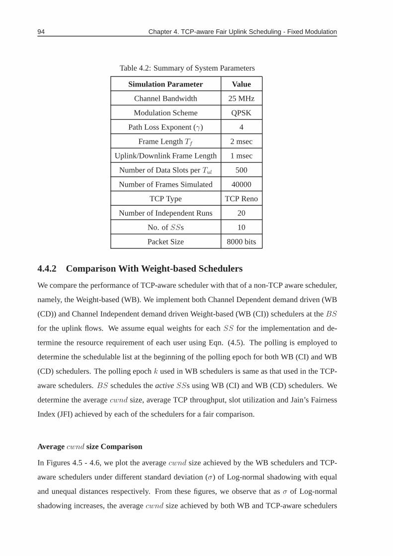
94 Chapter 4. TCP-aware Fair Uplink Scheduling - Fixed Modulation
Table 4.2: Summary of System Parameters
Simulation Parameter Value
Channel Bandwidth 25 MHz
Modulation Scheme QPSK
Path Loss Exponent (γ) 4
Frame LengthTf 2 msec
Uplink/Downlink Frame Length 1 msec
Number of Data Slots perTul 500
Number of Frames Simulated 40000
TCP Type TCP Reno
Number of Independent Runs 20
No. ofSSs 10
Packet Size 8000 bits
4.4.2 Comparison With Weight-based Schedulers
We compare the performance of TCP-aware scheduler with thatof a non-TCP aware scheduler,
namely, the Weight-based (WB). We implement both Channel Dependent demand driven (WB
(CD)) and Channel Independent demand driven Weight-based (WB (CI)) schedulers at theBS
for the uplink flows. We assume equal weights for eachSS for the implementation and de-
termine the resource requirement of each user using Eqn. (4.5). The polling is employed to
determine the schedulable list at the beginning of the polling epoch for both WB (CI) and WB
(CD) schedulers. The polling epochk used in WB schedulers is same as that used in the TCP-
aware schedulers.BS schedules theactiveSSs using WB (CI) and WB (CD) schedulers. We
determine the averagecwnd size, average TCP throughput, slot utilization and Jain’s Fairness
Index (JFI) achieved by each of the schedulers for a fair comparison.
Averagecwnd size Comparison
In Figures 4.5 - 4.6, we plot the averagecwnd size achieved by the WB schedulers and TCP-
aware schedulers under different standard deviation (σ) of Log-normal shadowing with equal
and unequal distances respectively. From these figures, we observe that asσ of Log-normal
shadowing increases, the averagecwnd size achieved by both WB and TCP-aware schedulers

4.4. Experimental Evaluation of TCP-aware Schedulers 95
30 40 50 60 70 80 901.4
1.5
1.6
1.7
1.8
Maximum cwnd (cwndMax
)
Avg
. TC
P T
hrou
ghpu
t (in
106 b
ps)
Equal Distances, Without Deadline, σ=8 dB
TWUS
Figure 4.4: Average TCP Throughput vs.cwndMax, with Fixed Modulation
decreases. We also observe that the averagecwnd size achieved by the TCP-aware schedulers
are higher than that of WB schedulers for all shadowing cases. In Figure 4.7, we plot the
percentage increase in the averagecwnd size by the TCP-aware schedulers over WB schedulers
under different shadowing. From this figure, we observe thatas theσ of Log-normal shadowing
increases, the gain incwnd size also increases. The gain in averagecwnd size of TWUS over
WB (CD) varies between 21% to 34%, whereas it varies between 37% to 88% for TWUS
over WB (CI). Though we have illustrated the results for equal distance experiments, similar
comparisons are also valid for unequal distance experiments. We also observe that the average
cwnd size achieved by the DTWUS is more than that of TWUS. As discussed before, by using
TCP timeouts in scheduling, the chances of reducing thecwnd size to one is minimized. This
results in increase in averagecwnd size.
We also compare the performance of WB (CD) and WB (CI) schedulers. From Figures
4.5 - 4.6, we observe that the averagecwnd size achieved by the WB (CD) scheduler is more
than that of WB (CI) scheduler, irrespective of distances. Since WB (CD) scheduler is channel
dependent, the slots allocated toSSs are better utilized. This ensures less slot idleness in WB
(CD) as compared to WB (CI) scheduler. Therefore, the average cwnd size achieved in WB
(CD) scheduler is more than that of WB (CI) scheduler.

96 Chapter 4. TCP-aware Fair Uplink Scheduling - Fixed Modulation
4 6 8 10 120
5
10
15
20
25
30
35
Log−normal Shadowing (σ in dB)
Avg
. Con
gest
ion
Win
dow
Siz
e (in
Pkt
s)Fixed Modulation, Equal Distances, cwnd
Max=60
WB (CI)WB (CD)TWUSDTWUS
Figure 4.5: Averagecwnd size Comparison - Fixed Modulation, Equal Distances
4 6 8 10 120
5
10
15
20
25
30
35
Log−normal Shadowing (σ in dB)
Avg
. Con
gest
ion
Win
dow
Siz
e (in
Pkt
s)
Fixed Modulation, Unequal Distances, cwndMax
=60
WB (CI)WB (CD)TWUSDTWUS
Figure 4.6: Averagecwnd size Comparison - Fixed Modulation, Unequal Distances

4.4. Experimental Evaluation of TCP-aware Schedulers 97
4 6 8 10 120
10
20
30
40
50
60
70
80
90
100
Log−normal Shadowing (σ in dB)
Gai
n in
Avg
. Con
gest
ion
Win
dow
Siz
e (in
%)
Fixed Modulation, Equal Distances, cwndMax
=60
TWUS − WB (CD)TWUS − WB (CI)
Figure 4.7: Gain incwnd size of TWUS over WB Schedulers - Equal Distances
Average Throughput Comparison
We also compare the average TCP throughput achieved by the schedulers. For TCP throughput
determination, we consider the number of successful transmitted packets only and do not con-
sider retransmissions. In Figures 4.8 - 4.9, we plot the average TCP throughput obtained by the
TCP-aware schedulers and WB schedulers under different shadowing and distances. We also
plot the gain in average TCP throughput achieved by the TCP-aware scheduler over the WB
schedulers in Figure 4.10. The improvements observed in TCPthroughput is similar to that of
the improvement in averagecwnd size illustrated in Figure 4.7. We also observe that the gainin
average TCP throughput of TWUS over WB (CI) varies between 39% to 97%, whereas it varies
between 24% to 42% for TWUS over WB (CD).

98 Chapter 4. TCP-aware Fair Uplink Scheduling - Fixed Modulation
4 6 8 10 120
0.5
1
1.5
2
2.5
Log−normal Shadowing (σ in dB)
Ave
rage
Thr
ough
put (
in 1
06 bps
)Fixed Modulation, Equal Distances, cwnd
Max=60
WB (CI)WB (CD)TWUSDTWUS
Figure 4.8: TCP Throughput Comparison - Fixed Modulation, Equal Distances
4 6 8 10 120
0.5
1
1.5
2
2.5
Log−normal Shadowing (σ in dB)
Ave
rage
Thr
ough
put (
in 1
06 bps
)
Fixed Modulation, Unequal Distances, cwndMax
=60
WB (CI)WB (CD)TWUSDTWUS
Figure 4.9: TCP Throughput Comparison - Fixed Modulation, Unequal Distances

4.4. Experimental Evaluation of TCP-aware Schedulers 99
4 6 8 10 120
10
20
30
40
50
60
70
80
90
100
110
120
Log−normal Shadowing (σ in dB)
Gai
n in
TC
P T
hrou
ghpu
t (in
%)
Fixed Modulation, Equal Distances, cwndMax
=60
TWUS − WB (CD)TWUS − WB (CI)
Figure 4.10: Gain in TCP Throughput of TWUS over WB Schedulers - Equal Distances
Fairness Comparison
To compare the fairness of TCP-aware schedulers with that ofWB schedulers, we determine
Jain’s Fairness Index (JFI) for the amount of data transmitted by eachSS considering equal
and unequal distances betweenSSs and theBS. We plot the variation of JFI thus determined
for different values ofσ of the Log-normal shadowing in Figures 4.11 - 4.12. From these
figures, we observe that the JFI is higher than 91% under all shadowing cases. JFI of TCP-
aware schedulers are close to 99% in the equal distance experiment, whereas it varies between
91% to 98% in the unequal distance experiment. This illustrates that the TCP-aware scheduling
schemes are fair under various channel fading conditions. We also observe that the JFI of both
TCP-aware and WB schedulers remains constant under different σ of Log-normal shadowing.
We observe that TCP-aware schedulers outperform WB schedulers with JFI as performance
metric. JFI obtained by the TCP-aware schedulers are at least 5% above that obtained by the
WB (CI) scheduler, whereas it is very close to that achieved by WB (CD) scheduler. Since
the WB (CI) scheduler is channel independent, the JFI achieved by this scheduler is low as
compared to other schedulers. Moreover, unlike other schedulers (TWUS, DTWUS and WB
(CD)), JFI of WB (CI) decreases as the shadowing increases.

100 Chapter 4. TCP-aware Fair Uplink Scheduling - Fixed Modulation
4 6 8 10 120.8
0.82
0.84
0.86
0.88
0.9
0.92
0.94
0.96
0.98
1
Log−normal Shadowing (σ in dB)
Jain
’s F
airn
ess
Inde
x (D
ata
Tra
nsm
itted
)
Fixed Modulation, Equal Distances, cwndMax
=60
WB (CI)WB (CD)TWUSDTWUS
Figure 4.11: Jain’s Fairness Index Comparison - Fixed Modulation, Equal Distances
4 6 8 10 120.8
0.82
0.84
0.86
0.88
0.9
0.92
0.94
0.96
0.98
1
Log−normal Shadowing (σ in dB)
Jain
’s F
airn
ess
Inde
x (D
ata
Tra
nsm
itted
)
Fixed Modulation, Unequal Distances, cwndMax
=60
WB (CI)WB (CD)TWUSDTWUS
Figure 4.12: Jain’s Fairness Index Comparison - Fixed Modulation, Unequal Distances

4.4. Experimental Evaluation of TCP-aware Schedulers 101
4 6 8 10 120.8
0.82
0.84
0.86
0.88
0.9
0.92
0.94
0.96
0.98
1
Log−normal Shadowing (σ in dB)
Jain
’s F
airn
ess
Inde
x (S
lots
Ass
igne
d)Fixed Modulation, Equal Distances, cwnd
Max=60
WB (CI)WB (CD)TWUSDTWUS
Figure 4.13: Jain’s Fairness Index Comparison - Fixed Modulation, Equal Distances
4 6 8 10 120.8
0.82
0.84
0.86
0.88
0.9
0.92
0.94
0.96
0.98
1
Log−normal Shadowing (σ in dB)
Jain
’s F
airn
ess
Inde
x (S
lots
Ass
igne
d)
Fixed Modulation, Unequal Distances, cwndMax
=60
WB (CI)WB (CD)TWUSDTWUS
Figure 4.14: Jain’s Fairness Index Comparison - Fixed Modulation, Unequal Distances

102 Chapter 4. TCP-aware Fair Uplink Scheduling - Fixed Modulation
We also compare the fairness of the schedulers based on the number of slots assigned to
different SSs under different shadowing. For this, we determine the JFI in number of slots
assigned and repeat the same for both equal and unequal distance cases. We plot the JFI thus
obtained in Figures 4.13 - 4.14. From these figures, we observe that JFI for the number of slots
assigned remains above 90% in all experiments. These results show similar trends with that
illustrated in Figures 4.11 - 4.12.
Slot Utilization and Idleness Comparison
We also investigate the slot utilization of the TCP-aware schedulers and compare it with WB
schedulers. For this, we plot the percentage of slot utilization of TCP-aware as well as WB
schedulers under different shadowing in Figures 4.15 - 4.16. From these figures, we observe
that the slot utilization of TCP-aware schedulers is more than that of WB schedulers. We also
observe that the utilization of TWUS scheduler is more than that of DTWUS scheduler and the
utilization of WB (CD) scheduler is more than that of WB (CI) scheduler. For the equal distance
experiment (Figure 4.15), slot utilization of TWUS and DTWUS scheduler varies between 84%
to 90%, whereas that of WB (CD) varies between 60% to 75% and WB(CI) varies between
46% to 68%. We observe similar trends for the unequal distance experiments (Figure 4.16).
From Figures 4.15 - 4.16, we also observe that the slot utilization of WB (CI) schedulers
falls as low as 40% when the Log-normal shadowing increases.This is because, when the chan-
nel is under heavy shadowing, the probability of getting polled is very low and the probability
of not being scheduled is very high. This results in increasein delay in scheduling, which may
triggers TCP timeout and drop incwnd size thereby resulting in low utilization. Utilization of
slots can be further increased by adding different classes of traffic along with TCP.
Since the TCP-aware schedulers assign slots to aSS only if there is a requirement and
the number of slots assigned is proportional to the resourcerequirement, the percentage of slot
idleness is negligible, whereas it is not so in WB schedulers. We plot the slot idleness of WB
schedulers at various Log-normal shadowing in Figures 4.17- 4.18. From these figures, we
observe that the slot idleness in WB (CI) scheduler is more than that of WB (CD) scheduler.
This results in higher averagecwnd size and average TCP throughput for WB (CD) scheduler
as compared to WB (CI) scheduler, explained in Figures 4.7 and 4.10.
We also compare the performance of TCP-aware schedulers with that of a RR scheduler,
in the next section.
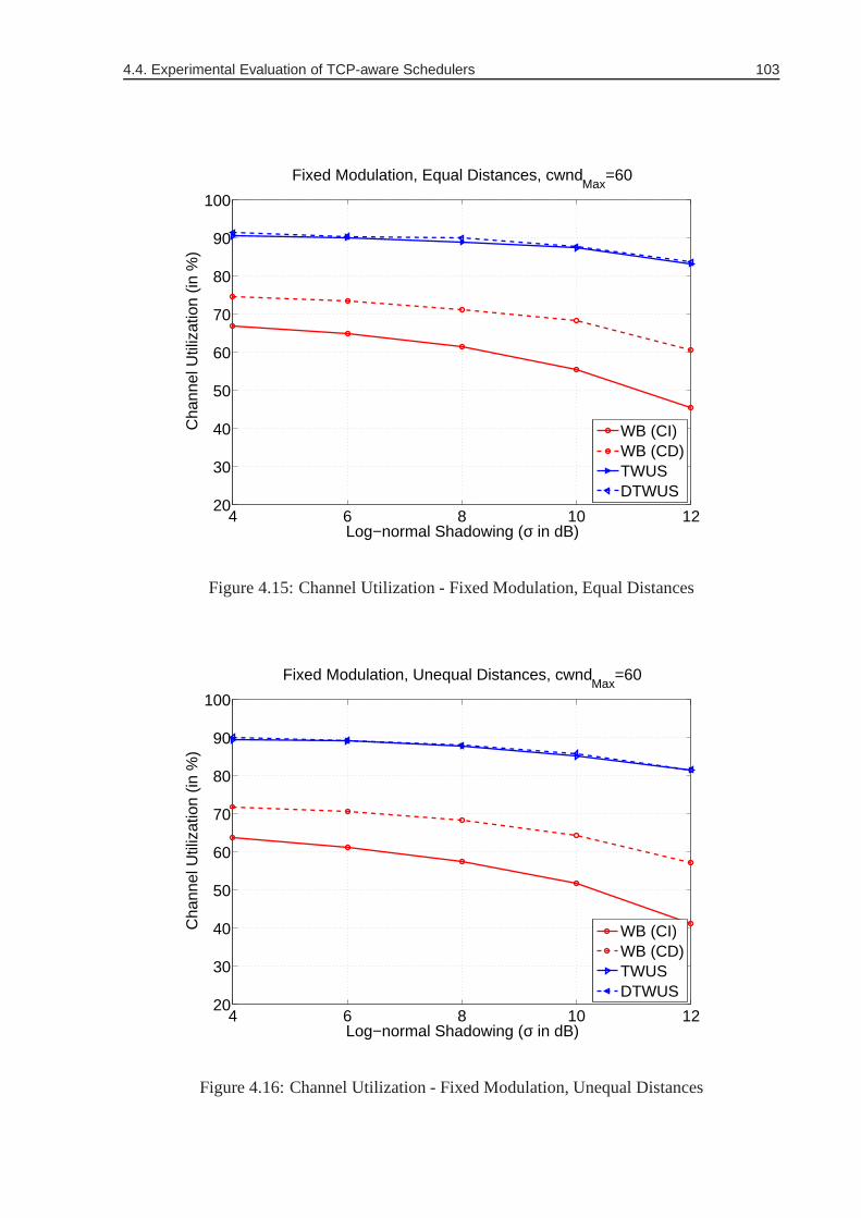
4.4. Experimental Evaluation of TCP-aware Schedulers 103
4 6 8 10 1220
30
40
50
60
70
80
90
100
Log−normal Shadowing (σ in dB)
Cha
nnel
Util
izat
ion
(in %
)Fixed Modulation, Equal Distances, cwnd
Max=60
WB (CI)WB (CD)TWUSDTWUS
Figure 4.15: Channel Utilization - Fixed Modulation, EqualDistances
4 6 8 10 1220
30
40
50
60
70
80
90
100
Log−normal Shadowing (σ in dB)
Cha
nnel
Util
izat
ion
(in %
)
Fixed Modulation, Unequal Distances, cwndMax
=60
WB (CI)WB (CD)TWUSDTWUS
Figure 4.16: Channel Utilization - Fixed Modulation, Unequal Distances

104 Chapter 4. TCP-aware Fair Uplink Scheduling - Fixed Modulation
4 6 8 10 120
5
10
15
20
25
30
Log−normal Shadowing (σ in dB)
Slo
t Idl
enes
s (in
%)
Fixed Modulation, Equal Distances, cwndMax
=60
WB (CI)WB (CD)
Figure 4.17: Slot Idleness - Fixed Modulation, Equal Distances
4 6 8 10 120
5
10
15
20
25
30
Log−normal Shadowing (σ in dB)
Slo
t Idl
enes
s (in
%)
Fixed Modulation, Unequal Distances, cwndMax
=60
WB (CI)WB (CD)
Figure 4.18: Slot Idleness - Fixed Modulation, Unequal Distances

4.5. Discussions 105
4.4.3 Comparison with Round Robin Scheduler
We also implement a RR scheduler at theBS for comparison with TCP-aware schedulers. RR
scheduler also determines the schedulable set at the beginning of the polling. The polling epoch
k used in RR scheduler is same as that used in the TCP-aware schedulers. In RR scheduler, the
BS schedules the activeSSs in every frame in a round robin manner. We compare the average
cwnd size and average TCP throughput achieved by the RR as well as TCP-aware schedulers.
In Figure 4.19, we plot the averagecwnd size under different shadowing with fixed modulation.
From this figure, we observe that the averagecwnd size achieved by the TCP-aware schedulers
are higher than that of RR schedulers for all shadowing cases. We also observe that as theσ of
Log-normal shadowing increases, the averagecwnd size achieved by both RR and TCP-aware
schedulers decreases. We also plot the average TCP throughput achieved by both RR and TCP-
aware schedulers in Figure 4.20. From this figure, we observethat the average TCP throughput
achieved by the TCP-aware schedulers is more as compared to that of RR schedulers. From
Figure 4.19, we observe that both the averagecwnd size and TCP throughput achieved by
DTWUS is more than that of TWUS. Though we have illustrated the results for equal distance
experiments, similar results are also valid for unequal distance experiments.
We also combine the comparisons of the performance of TCP-aware schedulers with that
of RR and WB schedulers. We plot the gain incwnd size and TCP throughput achieved in Fig-
ures 4.21 - 4.22. From these figures, we observe that the improvement of TCP-aware scheduler
over WB schedulers is more as compared to that of the improvement over RR scheduler. Since
DTWUS scheduler performs better than that of TWUS scheduler, we only plot the comparisons
of TWUS scheduler with that of RR and WB schedulers. Though wehave illustrated the results
for equal distance experiments, similar results are also valid for unequal distance experiments.
4.5 Discussions
In this chapter, we have proposed TCP-aware uplink scheduling schemes with fixed modula-
tion for a multipoint-to-point wireless network. We have performed extensive simulations and
compare the performance of the TCP-aware schedulers with other popular wire-line schedulers
such as Round Robin scheduler and Weight-based schedulers.In the next chapter, we incorpo-
rate adaptive modulation at the PHY layer and propose adaptive modulation based TCP-aware
scheduling schemes.

106 Chapter 4. TCP-aware Fair Uplink Scheduling - Fixed Modulation
4 6 8 10 120
5
10
15
20
25
30
35
Log−normal Shadowing (σ in dB)
Avg
. Con
gest
ion
Win
dow
Siz
e (in
Pkt
s)Fixed Modulation, Equal Distances, cwnd
Max=60
RRTWUSDTWUS
Figure 4.19: Comparison of TCP-aware Schedulers with RR Scheduler - Fixed Modulation,Equal Distances
4 6 8 10 120
0.5
1
1.5
2
2.5
Log−normal Shadowing (σ in dB)
Ave
rage
Thr
ough
put (
in 1
06 bps
)
Fixed Modulation, Equal Distances, cwndMax
=60
RRTWUSDTWUS
Figure 4.20: Comparison of TCP-aware Schedulers with RR Scheduler - Fixed Modulation,Equal Distances

4.5. Discussions 107
4 6 8 10 120
10
20
30
40
50
60
70
80
90
100
Log−normal Shadowing (σ in dB)
Gai
n in
Avg
. Con
gest
ion
Win
dow
Siz
e (in
%)
Fixed Modulation, Equal Distances, cwndMax
=60
TWUS − WB (CD)TWUS − WB (CI)TWUS − RR
Figure 4.21: Gain incwnd size of TWUS over RR and WB Schedulers - Equal Distances
4 6 8 10 120
10
20
30
40
50
60
70
80
90
100
110
120
Log−normal Shadowing (σ in dB)
Gai
n in
TC
P T
hrou
ghpu
t (in
%)
Fixed Modulation, Equal Distances, cwndMax
=60
TWUS − WB (CD)TWUS − WB (CI)TWUS − RR
Figure 4.22: Gain in TCP Throughput of TWUS over RR and WB Schedulers - Equal Distances

Chapter 5
TCP-aware Fair Uplink Scheduling -
Adaptive Modulation
In the previous chapter, we have proposed fixed modulation based TCP-aware fair uplink schedul-
ing schemes in a multipoint-to-point wireless network. However, to achieve high spectral effi-
ciency on fading channels, adaptive modulation and coding (AMC) can be used. Using AMC,
aBS can choose a suitable modulation and coding scheme with the availableSNR, such that
the overall system capacity is increased. Therefore, we incorporate AMC in the proposed TCP-
aware uplink scheduling algorithm. We also implement TCP-aware scheduling in the uplink
of a multipoint-to-point IEEE 802.16 network and investigate its performance through exhaus-
tive simulations. We compare the performance of TCP-aware uplink schedulers with adaptive
modulation and fixed modulation. In addition, we compare theperformance of TCP-aware
schedulers with that of Weight-based (WB) and Round Robin (RR) schedulers taking adaptive
modulation into consideration.
In Section 5.1, we discuss the system model of the TCP-aware schedulers. In Section
5.2, we present both TCP Window-aware Uplink Scheduling scheme and Deadline-based TCP
Window-aware Uplink Scheduling scheme and illustrate the slot assignment methods. In Sec-
tion 5.3, we discuss the implementation of TCP-aware schedulers in an IEEE 802.16 network.
In Section 5.4, we discuss the experimental set up and present the results. These results demon-
strate the efficiency of the proposed algorithm. In Section 5.5, we present TCPsend rate or
average throughput determination of TCP-aware uplink schedulers in an IEEE 802.16 network
and validate the analytical results with the simulation results. We discuss the fairness properties
109

110 Chapter 5. TCP-aware Fair Uplink Scheduling - Adaptive Modulation
of TCP-aware schedulers in Section 5.6.
5.1 System Model
The system model considered in this chapter is an extension of the system model that has been
described in Section 4.2. As discussed in the previous chapter, we consider a multipoint-to-
point wireless network, where multipleSSs are connected to oneBS, as illustrated in Figure
5.1 (same as Figure 4.2). We incorporate adaptive modulation and coding at the PHY layer.
As discussed before, packets can be successfully received if SNRi ≥ SNRth. The value
of SNRth depends upon the modulation and coding scheme used at the PHYlayer. The maxi-
mum data rate attainable on the channel depends upon the modulation scheme and coding used.
SS1
SS2
SSN
BS
cwnd1
cwnd2
cwndN
F low2
F low
N
F low1
TCP Traffic Sources
TC
PS
inks
Figure 5.1: Multipoint-to-Point Framework with TCP-basedApplications
5.2 Uplink Scheduling with Adaptive Modulation
LetRi denote the rate of transmission betweenSSi and theBS. Since wireless channel is time
varying and the channel state changes from frame to frame, the modulation scheme suitable
for that channel state also changes from frame to frame. Hence,Ri(n) changes from frame to
frame, withn being the frame index. Thus, defining quantum size in terms ofnumber of slots
assigned at the beginning of a polling epoch is not appropriate. We therefore, introduceRi(n)
in the definition of the quantum size as follows:

5.2. Uplink Scheduling with Adaptive Modulation 111
Q(0) =RminNsTs
M,
Q(n) =1
M
∑
i∈Lsch
F lagi(n− 1) × Ri(n− 1) ×Ni(n− 1) × Ts, ∀i ∈ Lsch, ∀n ≥ 1,(5.1)
whereRmin is the minimum rate of transmission among all modulation schemes. From the
above discussion, we observe thatQ varies from frame to frame of a polling epoch when the
PHY layer employs AMC, whereasQ is kept constant for a polling epoch when the PHY layer
employs fixed modulation.
Similar to the classifications of the TCP-aware scheduler that has been proposed in the pre-
vious chapter, we classify the scheduling schemes into (i) TCP Window-aware Uplink Schedul-
ing (TWUS-A) with Adaptive Modulation; and (ii) Deadline-based TCP Window-aware Uplink
Scheduling (DTWUS-A) with Adaptive Modulation. We discussthe details of the scheduling
algorithms in the subsequent sections.
5.2.1 Slot Allocation using TCP Window-aware Uplink Scheduling with
Adaptive Modulation
This scheme is an extension of TWUS algorithm proposed in Section 4.3.2. The basic operation
of it does not change significantly. Since the rate of transmission of differentSSs are different,
with the same number of slots, aSS with a higher transmission rate can transmit more number
of packets as compared to anotherSS with a relatively lower transmission rate. Therefore, we
introduceRi(n) into the resource requirementDi(n) and the deficit counterDCi(n). We update
the resource requirementDi(n) of each schedulableSS in a framen as follows:
Di(0) = cwndi × PL,
Di(n) = cwndi × PL− Txi(n− 1)
= Di(n− 1) − F lagi(n− 1) ×Ni(n− 1) ×Ri(n− 1) × Ts, ∀n ≥ 1.
(5.2)
We also update the deficit counterDCi(n) as follows:
DCi(0) = 1,
DCi(n) = DCi(n− 1) +Q(n) − F lagi(n− 1) ×Ri(n− 1) ×Ni(n− 1) × Ts, ∀i ∈ Lsch,
∀n ≥ 1.
(5.3)

112 Chapter 5. TCP-aware Fair Uplink Scheduling - Adaptive Modulation
As discussed before, the deficit counter can take a positive or negative value. Hence, we
use scaled deficit counterdci(n) for weight determination. The scaled deficit counter is updated
in a manner similar to that of Eqn. (4.7). After determining the resource requirement and the
scaled deficit counter, theBS determines the weights of eachSS for assigning time slots. The
weights are determined only for the active set members. For all otherSSs, the weights are zero.
TheBS determines weights of active setSSs using the following equation:
Wi(n) =
Di(n)Ri(n)
× dci(n)Ri(n)
∑
j∈Lactive
Dj(n)
Rj(n)×
dcj(n)
Rj(n)
, ∀i ∈ Lactive, ∀n ≥ 1. (5.4)
Eqn. (5.4) essentially determines a weightWi(n) in framen that is directly proportional
to the normalized (with respect to rateRi(n)) product of the scaled deficit counter and resource
requirement. As discussed before, since, the rate of transmission is different for differentSSs,
with the same number of slots, aSS with a higher transmission rate can transmit more num-
ber of packets as compared to anotherSS with a relatively smaller transmission rate. Hence,
allocating time slots in proportion only toDi(n) (or cwndi) may result in unfairness among
theSSs. We useRi(n) in weight determination to ensure fairness among theSSs. After the
determination of weights, theBS assigns slots toSSi, ∀i ∈ Lactive in framen using:
Ni(n) =1
Ts× min
{Wi(n) × Tf
∑
j∈LactiveWj(n)
,Di(n)
Ri(n)
}
, ∀i ∈ Lactive, ∀n ≥ 1. (5.5)
The first term in the braces of Eqn. (5.5) corresponds to the number of slots in proportion
to the weightWi(n), while the second term corresponds to the number of slots in proportion to
the resource requirementDi(n) of SSi. By using themin function in the above equation, the
BS restricts the maximum number of slots assigned to anySS by its requirement. This ensures
maximum slot utilization.
In the next section, we incorporate TCP timeout informationduring scheduling.
5.2.2 Slot Assignments using Deadline-based TCP Window-aware Uplink
Scheduling with Adaptive Modulation
In this scheme, the method of determination of resource requirement, deficit counter and scaled
deficit counter are similar to that defined in TWUS-A scheduler proposed in Section 5.2.1.

5.3. Implementation of TCP-aware Scheduling 113
In addition to that we also use the TCP timeout information ofthe active flows during the
scheduling process. To keep a track of the TCP timeout, we define deadline counterdi(n). The
update deadline counter update follows that of Eqn. (4.10)1.
After determining the scaled deficit counters as in Eqn. (4.7) and deadlines as in Eqn.
(4.10), theBS determines the weightWi(n) of SSi in framen using the following equation:
Wi(n) =
Di(n)Ri(n)
× dci(n)Ri(n)
/di(n)∑
j∈Lactive
Dj(n)
Rj(n)×
dcj(n)
Rj(n)/dj(n)
, ∀i ∈ Lactive, ∀n ≥ 1. (5.6)
Eqn. (5.6) is similar to Eqn. (5.4) except for the deadlinedi(n). The use of the deadline
in weight determination ensures that the weight of aSS that has a smaller deadline is higher as
compared to that of anotherSS which has a larger deadline. After the determination of weights,
the number of slots assigned toSSi, ∀i ∈ Lactive in framen is determined using Eqn. (5.5).
The pseudo-code of the proposed schedulers TWUS-A and DTWUS-A is presented in
Algorithm 2. We have combined both schedulers by usingF lagdeadline, which is set to one for
DTWUS-A and is set to zero for TWUS-A.
5.3 Implementation of TCP-aware Scheduling
We consider TDD based IEEE 802.16 network, in which each frame of durationTf is divided
into uplink and downlink subframes of durationsTul andTdl respectively. We consider adap-
tive modulation scheme at the PHY layer. We employ QPSK, 16-QAM, 64-QAM modulation
schemes as per the standard. Though the standard defines maximum baud rate, modulation
schemes to be used and maximum data rate possible for WirelessMAN-SC interface, it does not
specify theSNR thresholds for choosing different modulation schemes to beused.
The maximum data rate attainable for an Additive White Gaussian Noise (AWGN) channel
can be expressed as:R = B × log2(1 + MI × SNR), whereR is the maximum attainable
data rate andMI is the modulation index. Note thatMI = −φ1
log(φ2BER), whereφ1 andφ2 are
constants depending upon the modulation schemes [39]. Since the standard specifies data rates
to be used, for a particular modulation scheme,SNRth should satisfy:
1This scheme is also an extension of DTWUS scheme explained inSection 4.3.3.

114 Chapter 5. TCP-aware Fair Uplink Scheduling - Adaptive Modulation
SNR =2
RB − 1
MI
=(1 − 2
RB ) × ln(5pb)
1.5, if
R
B< 4
=(1 − 2
RB ) × ln(0.5pb)
1.5, if
R
B≥ 4,
(5.7)
wherepb is the target bit error rate. Using Eqn. (5.7), we determineSNRth for target BERs
of 10−5 and10−6 for a channel bandwidth (B) of 25 MHz. These are given in Table 5.1 for
the data rate of 40, 80 and 120 Mbps for QPSK, 16-QAM and 64-QAMmodulation schemes
respectively.
Table 5.1: Modulation Schemes in the Uplink of WirelessMAN-SC IEEE 802.16 (ChannelBandwidth B = 25 MHz)
Modulation Data Rate RB
SNRth (dB) SNRth (dB)
Scheme R (Mbps) (bps/Hz) BER = 10−5 BER = 10−6
QPSK 40 1.6 11.27 12.18
16-QAM 80 3.2 17.33 18.23
64-QAM 120 4.8 23.39 24.14
In the proposed scheme,SSs are required to maintain a queue (per flow) at their interfaces.
Packets residing in the queue of aSS is served in a first-come first-serve basis. As per the
standard, it is possible for theBS to determine the channel state of eachSS. This information
is used by theBS to determine the schedulable set at the beginning of pollingand to update
the active set in every frame. At the beginning of every polling epoch, eachSS conveys its
requirements in terms of its current congestion window (cwndi) size and time left to reach TCP
timeout (TTOi) to theBS. BS in turn, determines the number of slots to be assigned based on
the resource requirement, deficit counter and deadline value of each schedulableSS and decides
the modulation scheme to be used on a frame by frame basis.BS conveys this information to
eachSS through the uplink map.BS also determines the polling epochk (as discussed in
Section 4.3.1) such that the system efficiency and fairness are maintained. The block diagram
of the proposed uplink scheduler is shown in Figure 5.2.

5.3. Implementation of TCP-aware Scheduling 115
Algorithm 3 :TCP-aware Uplink Scheduler with Adaptive Modulation1: while TRUEdo
2: DetermineLsch for the current polling epoch
3: F lagi(0)← 0 ∀i ∈ Lsch
4: Di(n)← cwndi × PL, DCi(0)← 1, dci(0)← 1, Wi(0)← 0, Ni(0)← 0 ∀i ∈ Lsch
5: if ShcedulerType = TWUS − A then
6: F lagdeadline = 0, di(0)← 1 ∀i ∈ Lsch
7: else
8: F lagdeadline = 1, di(0)← TTOi ∀i ∈ Lsch
9: end if
10: M ← |Lsch|
11: if n = 1 then
12: Q(0)← Rmin×Ns×Ts
M
13: end if
14: k ← mini{RTTi}, T ← kTf
15: Frame numbern← 1
16: while T > 0 do
17: Lactive ← φ
18: for all i ∈ Lsch do
19: if (SNRi(n) ≥ SNRth) Λ(Di(n− 1) > 1) then
20: Lactive ← Lactive ∪ {i}
21: DCi(n)← DCi(n− 1) +Q(n− 1)− Ri(n− 1)×Ni(n− 1)× Ts
22: if F lagdeadline = 1 then
23: di(n)← di(n− 1)
24: else
25: di(n)← 1
26: end if
27: else
28: Ri(n)← 0, Di(n)← Di(n− 1), DCi(n)← DCi(n− 1) +Q(n− 1)
29: if F lagdeadline = 1 then
30: di(n)← di(n− 1)− Tf
31: else
32: di(n)← 1
33: end if
34: if di(n) ≤ 0 then
35: di(n)← TOi
36: end if
37: Wi(n)← 0, Ni(n)← 0
38: end if
39: end for
40: for all i ∈ Lactive do
41: Di(n)← Di(n− 1)−Ni(n− 1)× Ri(n− 1)× Ts
42: dci(n)← DCi(n) + minj |DCj(n)|, ∀j ∈ Lactive
43: MapRi(n) to SNRi(n) in Table 5.1
44: Wi(n)←
Di(n)Ri(n)
×dci(n)Ri(n)
/di(n)
P
j∈Lactive(
Dj(n)
Rj(n)×
dcj(n)
Rj(n)/dj(n))
45: Ni(n)← 1Ts×min
„
Wi(n)×TfP
j∈LactiveWj(n)
,Di(n)Ri(n)
«
46: Q(n)← 1M
P
i∈LschRi(n− 1)×Ni(n− 1)× Ts
47: end for
48: T ← T − Tf , n← n+ 1
49: end while
50: end while

116 Chapter 5. TCP-aware Fair Uplink Scheduling - Adaptive Modulation
Weights
Computation+
Deficit Counter
Demand+
Computation
Tolerable Delay
Update
Scheduler
Scheduling Info
of ’k’
Polling+
Computation
Ni(n)Ri(n)
Di(n)
di(n)
dci(n)
Ni(n)
Modni(n)
Wi(n)
SS1
SS2
SSN
TTOi
cwndi
Figure 5.2: Block Diagram of TCP-aware Uplink Scheduler
5.4 Experimental Evaluation of TCP-aware Schedulers with
Adaptive Modulation
In this section, we describe simulation experiments that have been performed to evaluate TCP-
aware scheduling with adaptive modulation. All the simulations have been conducted using
implementations of TCP-aware scheduling with IEEE 802.16 setting in MATLAB [68]. We
consider a multipoint-to-point IEEE 802.16 based network where 10SSs are connected to a
centralizedBS as shown in Figure 5.1. We considerBER = 10−6 for the applications and use
theSNRths for selecting an appropriate modulation scheme as shown inTable 5.1. Except for
the addition of adaptive modulation and coding at the PHY layer, the experimental setup used
here is identical to that of Section 4.4. The system parameters used for simulations are presented
in Table 5.2. The value of each parameter observed has been averaged over 50 independent
simulation runs.
We conduct four sets of experiments based on distance (equaland unequal), and the pro-
posed schedulers (TWUS-A and DTWUS-A). For each set of experiment, we vary the standard
deviation (σ) of Log-normal shadowing between 4, 6, 8, 10 and 12 dB.

5.4. Experimental Evaluation of TCP-aware Schedulers with Adaptive Modulation 117
Table 5.2: Summary of System Parameters
Simulation Parameter Value
Channel Bandwidth 25 MHz
Adaptive Modulation Schemes QPSK, 16-QAM, 64-QAM
Bit Error Rate 10−6
Path Loss Exponent (γ) 4
Frame LengthTf 2 msec
Uplink/Downlink Frame Length 1 msec
Number of Data Slots perTul 500
Number of Frames Simulated 40000
TCP Type TCP Reno
Number of Independent Runs 20
No. ofSSs 10
Packet Size 8000 bits
5.4.1 Simulation Results
Impact of cwndMax
We perform experiments to determine the value ofcwndMax at which the TCP throughput satu-
rates and plot the results in Figure 5.3. For completeness, we plot the results of both TWUS and
TWUS-A with equal distances in this figure. From this figure, we observe that TCP through-
put remains constant (reaches saturation) once thecwndMax reaches 70 packets for TWUS-A,
whereas it is 60 packets for TWUS. We choosecwndMax = 70 for the TCP-aware schedulers
with adaptive modulation scheme in the rest of our experiments.
5.4.2 Comparison With Weight-based Schedulers
We also compare the performance of TCP-aware schedulers with that of WB (CI) and WB
(CD) schedulers taking adaptive modulation into consideration. We determine the resource
requirement of each user using Eqn. (5.2). Similar to the fixed modulation experiments, we
determine the averagecwnd size, average TCP throughput, slot utilization and Jain’s Fairness
Index (JFI) achieved by each of the schedulers for a fair comparison.

118 Chapter 5. TCP-aware Fair Uplink Scheduling - Adaptive Modulation
30 40 50 60 70 80 901.4
1.6
1.8
2
2.2
2.4
2.6
2.8
Maximum Congestion Window (cwndMax
)
Ave
rage
TC
P T
hrou
ghpu
t (in
106 b
ps)
Equal Distances, Without Deadline, σ=8 dB
TWUSTWUS−A
Figure 5.3: Average TCP Throughput vs.cwndMax
Averagecwnd size Comparison
In Figures 5.4 - 5.5, we plot the averagecwnd size achieved by the WB schedulers and TCP-
aware schedulers under different standard deviation (σ) of Log-normal shadowing with adaptive
modulation. The distance between theSSs and theBS are considered to be equal in Figure 5.4
and unequal in Figure 5.5. From these figures, we observe thatthe averagecwnd size achieved
by the TCP-aware schedulers is higher than that of WB schedulers for all shadowing cases. We
also observe that as standard deviation of Log-normal shadowing increases, the averagecwnd
size achieved by both WB and TCP-aware schedulers decreases. However, we observe that the
rate of decrease ofcwnd is more in adaptive modulation (Figures 5.4 - 5.5) than that in fixed
modulation (Figures 4.5 - 4.6).
In Figure 5.6, we plot the percentage increase in the averagecwnd size by the TCP-aware
schedulers over WB schedulers under different Log-normal shadowing. From this figure, we
observe that as the standard deviation (σ) of the Log-normal shadowing increases, the gain in
cwnd size also increases. Moreover, the gain incwnd size of TWUS-A over WB (CI) varies
between 22% to 50%, whereas it varies between 38% to 91% for TWUS-A over WB (CD).
Though we have illustrated the results for equal distance experiments, similar comparisons are
also valid for unequal distance experiments.

5.4. Experimental Evaluation of TCP-aware Schedulers with Adaptive Modulation 119
We also compare the performance of WB (CD) and WB (CI) schedulers with adaptive
modulations. From Figures 5.4 - 5.5, we observe that the averagecwnd size achieved by the
WB (CD) scheduler is more than that of WB (CI) scheduler, which is similar to that of the
fixed modulation (Figures 4.5 - 4.6). However, the difference in averagecwnd size achieved
by the WB (CD) scheduler and WB (CI) scheduler with adaptive modulation is higher than that
achieved with fixed modulation. Since scheduling in WB (CD) is channel dependent, it is more
adaptive than WB (CI) to the variable rates than the fixed rate.
4 6 8 10 120
5
10
15
20
25
30
35
40
45
Log−normal Shadowing (σ in dB)
Avg
. Con
gest
ion
Win
dow
Siz
e (in
Pkt
s)
Adaptive Modulation, Equal Distances, cwndMax
=70
WB (CI)WB (CD)TWUS−ADTWUS−A
Figure 5.4: Averagecwnd size Comparison - Adaptive Modulation, Equal Distances
Average Throughput Comparison
We also compare the average TCP throughput achieved by the schedulers with adaptive mod-
ulation schemes. In Figures 5.7 - 5.8, we plot the average TCPthroughput obtained by the
TCP-aware schedulers and WB schedulers under different shadowing and distances. We plot
the gain in average TCP throughput achieved by the TCP-awarescheduler over the WB sched-
ulers in Figure 5.9. The improvements observed in TCP throughput is similar to that of the
improvement in averagecwnd size illustrated in Figure 5.6. We also observe that the gainin
average TCP throughput of TWUS-A over WB (CI) varies between25% to 60%, whereas it
varies between 38% to 100% for TWUS-A over WB (CD).

120 Chapter 5. TCP-aware Fair Uplink Scheduling - Adaptive Modulation
4 6 8 10 120
5
10
15
20
25
30
35
40
45
Log−normal Shadowing (σ in dB)
Avg
. Con
gest
ion
Win
dow
Siz
e (in
Pkt
s)Adaptive Modulation, Unequal Distances, cwnd
Max=70
WB (CI)WB (CD)TWUS−ADTWUS−A
Figure 5.5: Averagecwnd size Comparison - Adaptive Modulation, Unequal Distances
4 6 8 10 120
10
20
30
40
50
60
70
80
90
100
Log−normal Shadowing (σ in dB)
Gai
n in
Avg
. Con
gest
ion
Win
dow
Siz
e (in
%)
Adaptive Modulation, Equal Distances, cwndMax
=70
TWUS−A − WB (CD)TWUS−A − WB (CI)
Figure 5.6: Gain incwnd size of TWUS-A over WB Schedulers - Equal Distances

5.4. Experimental Evaluation of TCP-aware Schedulers with Adaptive Modulation 121
4 6 8 10 120
0.5
1
1.5
2
2.5
3
3.5
Log−normal Shadowing (σ in dB)
Ave
rage
Thr
ough
put (
in 1
06 bps
)
Adaptive Modulation, Equal Distances, cwndMax
=70
WB (CI)WB (CD)TWUS−ADTWUS−A
Figure 5.7: TCP Throughput Comparison - Adaptive Modulation, Equal Distances
4 6 8 10 120
0.5
1
1.5
2
2.5
3
3.5
Log−normal Shadowing (σ in dB)
Ave
rage
Thr
ough
put (
in 1
06 bps
)
Adaptive Modulation, Unequal Distances, cwndMax
=70
WB (CI)WB (CD)TWUS−ADTWUS−A
Figure 5.8: TCP Throughput Comparison - Adaptive Modulation, Unequal Distances

122 Chapter 5. TCP-aware Fair Uplink Scheduling - Adaptive Modulation
4 6 8 10 120
10
20
30
40
50
60
70
80
90
100
110
120
Log−normal Shadowing (σ in dB)
Gai
n in
TC
P T
hrou
ghpu
t (in
%)
Adaptive Modulation, Equal Distances, cwndMax
=70
TWUS−A − WB (CD)TWUS−A − WB (CI)
Figure 5.9: Gain in TCP Throughput of TWUS-A over WB Schedulers - Equal Distances
Fairness Comparison
We also determine the JFI for the amount of data transmitted by eachSS and the number of
slots assigned to eachSS for the TCP-aware and WB schedulers with adaptive modulation. In
Figures 5.10 and 5.11, we plot the variation of JFI thus determined for different value ofσ of
Log-normal shadowing. From these figures, we observe that both TWUS-A and DTWUS-A are
fair under various shadowing conditions. Moreover, JFI obtained by TWUS-A and DTWUS-A
schedulers are higher than that of WB (CI) scheduler. However, JFI obtained by TWUS-A and
DTWUS-A schedulers are in the same range with that of WB (CD) scheduler. This is due to the
fact that WB (CD) is adaptive to the channel states and attempts to schedule the users in such
a manner that the amount of data transmitted by each user is the same. We also observe that
unlike fixed modulation, the JFI of TWUS-A and DTWUS-A decreases as standard deviation
of Log-normal shadowing increases. Though we have illustrated the results for equal distance
experiments, similar results are also valid for unequal distance experiments.
Slot Utilization and Idleness Comparison
We investigate the slot utilization of TWUS-A and DTWUS-A and compare it with WB (CD)
and WB (CI) schedulers. For this, we plot the percentage in slot utilization under different

5.4. Experimental Evaluation of TCP-aware Schedulers with Adaptive Modulation 123
4 6 8 10 120.8
0.82
0.84
0.86
0.88
0.9
0.92
0.94
0.96
0.98
1
Log−normal Shadowing (σ in dB)
Jain
’s F
airn
ess
Inde
x (D
ata
Tra
nsm
itted
)Adaptive Modulation, Equal Distances, cwnd
Max=70
WB (CI)WB (CD)TWUS−ADTWUS−A
Figure 5.10: Jain’s Fairness Index Comparison - Adaptive Modulation, Equal Distances
4 6 8 10 120.8
0.82
0.84
0.86
0.88
0.9
0.92
0.94
0.96
0.98
1
Log−normal Shadowing (σ in dB)
Jain
’s F
airn
ess
Inde
x (S
lots
Ass
igne
d)
Adaptive Modulation, Equal Distances, cwndMax
=70
WB (CI)WB (CD)TWUS−ADTWUS−A
Figure 5.11: Jain’s Fairness Index Comparison - Adaptive Modulation, Equal Distances

124 Chapter 5. TCP-aware Fair Uplink Scheduling - Adaptive Modulation
shadowing and distances in Figures 5.12 - 5.13. From these figures, we observe that the slot
utilization of TCP-aware schedulers is more than that of WB schedulers. We also observe
that the utilization of TWUS-A scheduler is more than that ofDTWUS-A scheduler and the
utilization of WB (CD) scheduler is more than that of WB (CI) scheduler. Moreover, the slot
utilization of TWUS-A and DTWUS-A scheduler varies between70% to 85%, whereas that of
WB (CI) and WB (CD) varies between 40% to 60%. Similar to the results obtained in the fixed
modulation experiments, in adaptive modulation, we also observe that the slot utilization of
WB (CI) scheduler falls as low as 40% when the standard deviation of Log-normal shadowing
increases. This is because, when the channel is under heavy shadowing, the probability of
getting polled is very low and the probability of not being scheduled in a frame is very high.
This results in congestion and drop incwnd size thereby resulting in low utilization. Utilization
of slots can be further increased by adding different classes of traffic along with TCP traffic.
We also compare the slot idleness of WB (CD) and WB (CI) schedulers with adaptive
modulation. We plot the slot idleness of WB schedulers underdifferentσ of Log-normal shad-
owing in Figures 5.14 - 5.15. From these figures, we observe that the slot idleness in WB (CI)
scheduler is more than that of WB (CD) scheduler. This results in higher averagecwnd size and
average TCP throughput for WB (CD) scheduler as compared to WB (CI) scheduler, observed
in Figures 5.6 - 5.9.
4 6 8 10 1220
30
40
50
60
70
80
90
100
Log−normal Shadowing (σ in dB)
Cha
nnel
Util
izat
ion
(in %
)
Adaptive Modulation, Equal Distances, cwndMax
=70
WB (CI)WB (CD)TWUS−ADTWUS−A
Figure 5.12: Channel Utilization - Adaptive Modulation, Equal Distances

5.4. Experimental Evaluation of TCP-aware Schedulers with Adaptive Modulation 125
4 6 8 10 1220
30
40
50
60
70
80
90
100
Log−normal Shadowing (σ in dB)
Cha
nnel
Util
izat
ion
(in %
)
Adpative Modulation, Unequal Distances, cwndMax
=70
WB (CI)WB (CD)TWUS−ADTWUS−A
Figure 5.13: Channel Utilization - Adaptive Modulation, Unequal Distances
4 6 8 10 120
5
10
15
20
25
30
Log−normal Shadowing (σ in dB)
Slo
t Idl
enes
s (in
%)
Adaptive Modulation, Equal Distances, cwndMax
=70
WB (CI)WB (CD)
Figure 5.14: Slot Idleness - Adaptive Modulation, Equal Distances

126 Chapter 5. TCP-aware Fair Uplink Scheduling - Adaptive Modulation
4 6 8 10 120
5
10
15
20
25
30
Log−normal Shadowing (σ in dB)
Slo
t Idl
enes
s (in
%)
Adpative Modulation, Unequal Distances, cwndMax
=70
WB (CI)WB (CD)
Figure 5.15: Slot Idleness - Adaptive Modulation, Unequal Distances
We also compare the performance of TCP-aware schedulers with that of a RR scheduler
with adaptive modulation in the next section.
5.4.3 Comparison with Round Robin Scheduler
We compare the performance of TCP-aware schedulers with that of a Round Robin (RR) sched-
uler taking adaptive modulation into consideration. Similar to the fixed modulation experiment,
we compare the averagecwnd size and average TCP throughput achieved by the RR as well
as TCP-aware schedulers. In Figures 5.16 and 5.17, we plot the averagecwnd size and TCP
throughput obtained respectively under different shadowing with adaptive modulation in con-
sideration. From these figures, we observe that the averagecwnd size as well as TCP thoughput
achieved by the TCP-aware schedulers are higher than that ofRR schedulers for all Log-normal
shadowing cases. Similar to the results obtained with fixed modulation, we also observe that
with adaptive modulation, as theσ of Log-normal shadowing increases, the averagecwnd size
as well as TCP throughput achieved by both RR and TCP-aware schedulers decreases. How-
ever, the rate of decrease ofcwnd and TCP throughput is more in adaptive modulation than
that in fixed modulation (Figures 4.19- 4.20). Though, we have illustrated the results for equal
distance experiments, similar results are also valid for unequal distance experiments.

5.4. Experimental Evaluation of TCP-aware Schedulers with Adaptive Modulation 127
4 6 8 10 120
5
10
15
20
25
30
35
40
45
Log−normal Shadowing (σ in dB)
Avg
. Con
gest
ion
Win
dow
Siz
e (in
Pkt
s)
Adaptive Modulation, Equal Distances, cwndMax
=70
RRTWUS−ADTWUS−A
Figure 5.16: Comparison of TCP-aware Schedulers with RR Scheduler - Adaptive Modulation,Equal Distances
4 6 8 10 120
0.5
1
1.5
2
2.5
3
3.5
Log−normal Shadowing (σ in dB)
Ave
rage
Thr
ough
put (
in 1
06 bps
)
Adaptive Modulation, Equal Distances, cwndMax
=70
RRTWUS−ADTWUS−A
Figure 5.17: Comparison of TCP-aware Schedulers with RR Scheduler - Adaptive Modulation,Equal Distances

128 Chapter 5. TCP-aware Fair Uplink Scheduling - Adaptive Modulation
We also combine the comparisons of the performance of TCP-aware schedulers with that
of RR and WB schedulers and plot the gain incwnd size and TCP throughput achieved in
Figures 5.18 - 5.19. Similar to the results obtained with fixed modulation, we also observe that
the improvement of TCP-aware scheduler over WB scheduler ismore as compared to that of
the improvement over RR scheduler. Since DTWUS-A schedulerperforms better than that of
TWUS-A scheduler, we only plot the comparisons of TWUS-A scheduler with that of RR and
WB schedulers. Though we have illustrated the results for equal distance experiments, similar
results are also valid for unequal distance experiments.
4 6 8 10 120
10
20
30
40
50
60
70
80
90
100
Log−normal Shadowing (σ in dB)
Gai
n in
Avg
. Con
gest
ion
Win
dow
Siz
e (in
%)
Adaptive Modulation, Equal Distances, cwndMax
=70
TWUS−A − WB (CD)TWUS−A − WB (CI)TWUS−A − RR
Figure 5.18: Gain incwnd size of TWUS-A over RR and WB Schedulers - Equal Distances
5.4.4 Adaptive Modulation vs. Fixed Modulation
From the simulation results presented in the previous section and in Section 4.4.1, we observe
that the amount of data transmitted by the users in adaptive modulation scheme is more as com-
pared to the amount of data transmitted in fixed modulation scheme. The average rate of trans-
mission is almost double (80-90%) in adaptive modulation scheme as compared to fixed modu-
lation scheme for similar conditions. The higher rate of transmission in adaptive modulation is
achieved by adding extra complexity in the transmitter and receiver structures atSSs. Adaptive
modulation scheme also increases averagecwnd size, resulting in higher TCP throughput. We

5.4. Experimental Evaluation of TCP-aware Schedulers with Adaptive Modulation 129
4 6 8 10 120
10
20
30
40
50
60
70
80
90
100
110
120
Log−normal Shadowing (σ in dB)
Gai
n in
TC
P T
hrou
ghpu
t (in
%)
Adaptive Modulation, Equal Distances, cwndMax
=70
TWUS−A − WB (CD)TWUS−A − WB (CI)TWUS−A − RR
Figure 5.19: Gain in TCP Throughput of TWUS-A over RR and WB Schedulers - Equal Dis-tances
also observe that thecwnd size changes at a slower time scale than the transmission rate. Due
to this reason, even though the rate of transmission increases by 80-90%, the averagecwnd size
improves only by 50-55%. Similar observations are also valid for TCP throughput increase. On
comparing the slot utilization of TCP-aware schedulers with fixed and adaptive modulations
(Figures 4.15 - 4.16 and 5.12 - 5.13), we also observe that schedulers with fixed modulation
scheme have higher slot utilization than schedulers with adaptive modulation scheme.
From both fixed as well as adaptive modulation experiments, we observe that as the stan-
dard deviation of the Log-normal shadowing increases, bothaveragecwnd and TCP throughput
decreases. However, the rate of decrease ofcwnd and TCP throughput is more in adaptive mod-
ulation than that in fixed modulation. We also observe that schedulers with fixed modulation
scheme have higher slot utilization than schedulers with adaptive modulation scheme.
5.4.5 Layer-2 and Layer-4 Fairness
In this section, we investigate both Layer-2 and Layer-4 fairness [66] of TCP-aware schedulers.
We use Jain’s Fairness Index as Layer-2 fairness index and use both Worst Case TCP Fairness
Index (WCTFI) and TCP Fairness Index (TFI) as Layer-4 fairness index. The details of Layer-2

130 Chapter 5. TCP-aware Fair Uplink Scheduling - Adaptive Modulation
and Layer-4 fairness index have been discussed in Section 2.4.
Since the TCP-aware schedulers perform better than the RR and WB schedulers in terms
of throughput and JFI, we present the Layer-2 and Layer-4 fairness only for the TCP-aware
schedulers. Since TWUS-A and DTWUS-A outperform RR scheduler, we observe that both
WCTFI and TFI are one for TWUS-A and DTWUS-A and hence the proposed scheduling
schemes are fair at the Transport layer too.
5.5 TCP Throughput Analysis
In this section, we first develop an analytical framework to determine the throughput of TCP-
based applications in a multipoint-to-point IEEE 802.16 network. The TCP throughput analysis
is based on [75], a seminal work which models TCP Reno performance by the average TCP
send rate or throughput. In [75], the authors have derived a closed form expression for the
steady statesend rate of TCP flow as a function of loss rate,RTT and TCP timeout. How-
ever, their model assumes a wired network where the packet losses are assumed to be due to
congestion in the network. Modelling of TCPsend rate for wireless broadband networks like
IEEE 802.16 requires the inclusion of the effect of MAC layerscheduling (which is absent in
wired network) and packet losses due to the time varying nature of the channel. In this chapter,
we incorporate the impact of scheduling at the MAC layer and wireless packet losses on the
send rate determination of TCP flows. We assume that the packets are of fixed sizes and are
transmitted at the granularity of TCP Packets instead of MACPDUs. This simplifies the com-
plexity due to fragmentation and packing in our analysis. Wealso ignore the impact of ARQ
mechanism for simplicity. Even though in the actual implementations of TCP,cwndi increases
by 1cwndi
each time an ACK is received, we do not consider this in our analysis. The reason is
as follows: we assume that thecwnd value does not change for oneRTT . Based on thecwndi
value received during polling, theBS assigns time slots. Hence, even though thecwndi change
during a polling epoch, it will not be conveyed to theBS. The change incwnd size is only
conveyed at the time of polling. We also assume that the time taken to transmit all packets of a
window is smaller than oneRTT . This means that there will be some idle periods, which we
exploit during scheduling.
As discussed in Section 4.1.1, scheduling at the MAC layer has an impact on thecwnd

5.5. TCP Throughput Analysis 131
variation. Unless aSS is polled, it will not be considered for scheduling in that polling epoch.
UnpolledSSs have to wait till the next polling epoch resulting delay in scheduling. We now
determine the average uplink delay of the TCP-aware schedulers.
5.5.1 Average Uplink Delay of TCP-aware Scheduling
Let cwndi(n) denote the congestion window ofSSi in framen. We assume that the resource
requirement of aSS does not change during a polling epoch (irrespective of whether aSS is
polled or not). Letk denote the polling epoch in number of frames. As discussed before, aSS
is successfully polled if it has a non zerocwnd size and itsSNR exceedsmin{SNRth}. Let
M denote the number ofSSs polled successfully in a polling epoch. LetN denote the total
number ofSSs. We assumeN to be fixed. The probability thatM out ofN users are polled at
any polling instant is given by:
p(M) =
(N
M
)
pM(1 − p)N−M , (5.8)
wherep is the probability thatSNRi ≥ min{SNRth}, for any SSi. The number ofSSs
scheduled in a frame will always be less than or equal toM , the number ofSSs in that polling
epoch. The expected number ofSSs polled successfully can be expressed as:
E[M ] =N∑
M=0
Mp(M),
=N∑
M=0
M
(N
M
)
pM(1 − p)N−M .
(5.9)
After determining the expected number ofSSs to be polled in any polling epoch, we
determine the number of frames that aSS needs to wait before getting polled. In TCP-aware
scheduling, if oneSS misses polling, it needs to wait again fork frames before obtaining
another chance of polling. Though the value of polling epochk depends on theRTT of the
flows, we assume fixedk in this section for simplicity.SSi gets polled successfully in the first
polling epoch with probabilityp, otherwise, it gets polled in the second polling epoch with
probability(1 − p)p and so on. Hence, the expected number of polling epochsL is:
E[L] =∞∑
L=1
Lp(1 − p)L−1 − 1. (5.10)
The expected number of frames that aSS waits before getting polled successfully is
E[L] × k × Tf . Once aSS is polled successfully, it gets scheduled in the first frame of the
polling epoch, but it may or may not be scheduled in the subsequent frames, since in every

132 Chapter 5. TCP-aware Fair Uplink Scheduling - Adaptive Modulation
frame theBS requires theSNR to exceedmin{SNRth} before scheduling. In the successive
frames,M ′ out ofM polled users are scheduled and the value ofM ′ varies from frame to frame
(M ′ ≤ M ≤ N). The expected number ofSSs successfully scheduled out ofM polled users is
determined as:
E[M ′/M ] =
M∑
M ′=0
M ′(M
M ′
)
pM′
(1 − p)M−M′
, (5.11)
and the expected number of users scheduled in a frame is expressed as:
E[M ′] =
N∑
M=0
E[M ′/M ]p(M),
=
N∑
M=0
(M∑
M ′=0
M ′(M
M ′
)
pM′
(1 − p)M−M′
)
p(M).
(5.12)
5.5.2 Determination of Uplink Scheduling Delay
After determining the expected number ofSSs successfully scheduled in each frame, we deter-
mine the average number of frames in which a polledSS gets scheduled. On an average, due
to TCP-aware scheduling a polledSS transmits inE[M ′]E[M ]
×k frames out ofk frames in a polling
epoch. Hence, the average time a polledSS remains idle (not scheduled) due to TCP-aware
scheduling is expressed as:
Twf =
(
1 −E[M ′]
E[M ]
)
kTf . (5.13)
Thus, the extra time that aSS waits due to scheduling in the uplink can be expressed as
the sum of polling delay and idleness during a polling epoch.The average uplink delay due to
TCP-aware scheduling can be expressed as:
Tuld = E[L] × k × Tf + Twf . (5.14)
5.5.3 TCPsend rate Determination
If a SS is polled successfully, then it has a chance of being scheduled in that polling epoch. It is
possible that theSS may not be able to transmit one window worth of data or may experience
triple dupacksor timeouts in that polling epoch. However, if aSS is not polled, the chance of

5.5. TCP Throughput Analysis 133
increasing its congestion window is minimal. Increase in congestion window only occurs, if it
receives a pendingACK.
From the above discussion, it is evident that TCP behavior does not change due to TCP-
aware scheduling. Instead it follows the behavior seen in wired network, except for the extra
delay due to polling (not due to scheduling) and wireless packet losses. The wireless packet
losses can be neglected due to adaptive modulation and rate adaptation in our framework. Thus
the only extra factor that we need to consider for TCPsend rate determination is the polling
delay.
As discussed in [75], the average TCPsend rate in a wired network can be expressed as:
Bw ≈ min
(
cwndMax
RTTw,
1
RTTw
√2bpw
3+ TOmin
(
1, 3√
3bpw
8
)
pw(1 + 32p2w)
)
,(5.15)
whereBw is the TCP end-to-end throughput for a wired network (in packets per unit time),b is
the number of TCP packets acknowledged by one ACK,RTTw is the average TCP round trip
time in a wired network (only due to congestion),pw is the wirelink loss probability andTO
is the average TCP timeout value. Since TCP does not differentiate between wireless loss and
congestion loss, we assume all losses are congestion lossesand determine the number of loss
indications. In TCP, since the congestion window size can grow uptocwndMax, maximum TCP
send rate is bounded bycwndMax
RTTw.
The end-to-end average TCP throughput orsend rate for IEEE 802.16 based network can
be expressed by incorporating polling delay. The round triptimeRTTwr in Eqn. (5.15) can be
modified as:
RTTwr = RTTw + E[L] × k × Tf . (5.16)
By replacingRTTw by RTTwr in Eqn. (5.15), end-to-end TCP throughput orsend rate
for IEEE 802.16 based network (Bwr) can be expressed as:
Bwr ≈ min
(
cwndMax
RTTwr,
1
RTTwr
√2bpw
3+ TOmin
(
1, 3√
3bpw
8
)
pw(1 + 32p2w)
)
.(5.17)

134 Chapter 5. TCP-aware Fair Uplink Scheduling - Adaptive Modulation
5.5.4 Validation of TCP Throughput
To validate the TCP throughput analysis and averagesend rate of TCP flows, we compare the
average TCPsend rate obtained in Eqn. (5.17) with our simulation results. We determine the
probability of loss (pw) similar to that of [75]. We consider both triple-duplicateACKs and TCP
timeouts as loss indications. Letpw be the ratio of the total number of loss indications to the total
number of packets transmitted. From simulations, we observe that the average probability (p)
thatSNRi ≥ min{SNRth} is 0.87,∀i ∈ I. Using Eqn. (5.16), we determineRTTwr. Then by
using the value ofRTTwr obtained using Eqn. (5.16) andpw obtained above, we determine the
average TCPsend rate (analytical) using Eqn. (5.17). The average uplink scheduling latency
for various channel conditions and equal (E) and unequal (U)distances are presented in Figures
5.20 - 5.23.
To verify our model, we determine average TCPsend rate for all four sets of experiments
(TWUS-A with equal and unequal distances, DTWUS-A with equal and unequal distances).
We plot the analytical and experimental TCP throughput at differentcwndMax in Figures 5.24
- 5.27. From these figures, we observe that the theoreticalsend rates determined using Eqn.
(5.17) and thesend rate obtained by our simulations are matching very closely.
4 6 8 10 120
5
10
15
20
25
30
Log−normal Shadowing (σ in dB)
Ave
rage
Upl
ink
Late
ncy
(in m
sec)
Fixed Modulation, Without Deadline, cwndMax
=60
TWUS (E)TWUS (U)
Figure 5.20: Average Uplink Scheduling Latency of TWUS

5.5. TCP Throughput Analysis 135
4 6 8 10 120
5
10
15
20
Log−normal Shadowing (σ in dB)
Ave
rage
Upl
ink
Late
ncy
(in m
sec)
Adaptive Modulation, Without Deadline, cwndMax
=70
TWUS−A (E)TWUS−A (U)
Figure 5.21: Average Uplink Scheduling Latency of TWUS-A
4 6 8 10 120
5
10
15
20
25
30
Log−normal Shadowing (σ in dB)
Ave
rage
Upl
ink
Late
ncy
(in m
sec)
Fixed Modulation, With Deadline, cwndMax
=60
DTWUS (E)DTWUS (U)
Figure 5.22: Average Uplink Scheduling Latency of DTWUS

136 Chapter 5. TCP-aware Fair Uplink Scheduling - Adaptive Modulation
4 6 8 10 120
5
10
15
20
Log−normal Shadowing (σ in dB)
Ave
rage
Upl
ink
Late
ncy
(in m
sec)
Adaptive Modulation, With Deadline, cwndMax
=70
DTWUS−A (E)DTWUS−A (U)
Figure 5.23: Average Uplink Scheduling Latency of DTWUS-A
30 40 50 60 70 80 900
0.5
1
1.5
2
2.5
3
3.5
Maximum Congestion Window (cwndMax
)
Ave
rage
TC
P T
hrou
ghpu
t (in
106 b
ps)
Adaptive Modulation, Equal Distances, Without Deadline, σ=8 dB
TWUS−A (Simulation)TWUS−A (Analysis)
Figure 5.24: Average TCP Throughput of TWUS-A at DifferentcwndMax - Equal Distances

5.5. TCP Throughput Analysis 137
30 40 50 60 70 80 900
0.5
1
1.5
2
2.5
3
3.5
Maximum Congestion Window (cwndMax
)
Ave
rage
TC
P T
hrou
ghpu
t (in
106 b
ps)
Adaptive Modulation, Equal Distances, With Deadline, σ=8 dB
DTWUS−A (Simulation)DTWUS−A (Analysis)
Figure 5.25: Average TCP Throughput of DTWUS-A at DifferentcwndMax - Equal Distances
30 40 50 60 70 80 900
0.5
1
1.5
2
2.5
3
3.5
Maximum Congestion Window (cwndMax
)
Ave
rage
TC
P T
hrou
ghpu
t (in
106 b
ps)
Adaptive Modulation, Unequal Distances, Without Deadline, σ=8 dB
TWUS−A (Simulation)TWUS−A (Analysis)
Figure 5.26: Average TCP Throughput of TWUS-A at DifferentcwndMax - Unequal Distances

138 Chapter 5. TCP-aware Fair Uplink Scheduling - Adaptive Modulation
30 40 50 60 70 80 900
0.5
1
1.5
2
2.5
3
3.5
Maximum Congestion Window (cwndMax
)
Ave
rage
TC
P T
hrou
ghpu
t (in
106 b
ps)
Adaptive Modulation, Unequal Distances, With Deadline, σ=8 dB
DTWUS−A (Simulation)DTWUS−A (Analysis)
Figure 5.27: Average TCP Throughput of DTWUS-A at DifferentcwndMax - Unequal Dis-tances
It has been investigated that the DRR scheduler proposed fora wired network is a long-
term fair scheduler [29]. Since the TCP-aware scheduler is avariant of DRR scheduler, it should
follow the basic properties of DRR scheduler. However, the TCP aware scheduler operates in a
multipoint-to-point wireless network and uses a polling method to select the list of schedulable
users. Therefore, even though it is a variant of DRR scheduler, its implementation requirements
are different from that of DRR scheduler. We therefore, investigate its properties in the next
section.
5.6 Properties of TCP-aware Schedulers
Since the TCP-aware scheduler with fixed modulation can be considered as a special case of
TCP-aware scheduler with adaptive modulation, we investigate the properties of TCP-aware
scheduler with adaptive modulation. Before analyzing the properties of TCP-aware scheduler
with adaptive modulation, we first investigate the properties of quantum sizeQ(n) and deficit
counterDCi(n).
Property 1. The maximum value of quantum sizeQ(n) is bounded bycwndMax.
In a polling epoch, since the resource requirement of aSS cannot exceed the maximum

5.6. Properties of TCP-aware Schedulers 139
congestion window size (cwndMax) defined by the protocol, the average amount of data trans-
mission perSS in a frame cannot exceedcwndMax. Hence, the quantum sizeQ(n) is bounded
by cwndMax. This can be verified from Eqn. (5.2) also.
Property 2. Deficit CounterDCi, ∀i ∈ I must satisfy:|DCi| ≤ cwndMax
At the beginning of the polling epoch, the deficit counterDCi(0) = 1. During a polling
epoch, the value of the deficit counter can become either positive or negative. From Eqn. (5.3),
we observe that if a schedulableSS is not assigned any slots in a polling epoch, then its deficit
counter will rise to the maximum value of the quantum sizeQ(n). SinceQ(n) is limited by
cwndmax, the deficit counter is also limited bycwndMax.
Contrary to the above, ifSSi is scheduled in one polling epoch such that its entire window
of data is transmitted, then the resource requirement ofSSi drops to zero. This will result in the
removal ofSSi from the active list. In this case, the deficit counter can reach−cwndMax, just
beforeSSi is withdrawn from the active set.
As discussed in Chapter 2, a good scheduling algorithm must guarantee fair share of the
network resources to each user over a certain time duration.For example, TCP-based appli-
cations are unfair over oneRTT . This is because, the rate of transmission of TCP-based ap-
plication is governed by itscwnd size. Sincecwnd sizes are different for different users over
oneRTT , the amount of packet transmitted by the TCP-based applications are different for
different users. This results in unfairness.
Therefore, the minimum duration over which TCP-aware schedule is fair depends upon
the polling epoch and TCP timeout value. Since in a polling epoch, the proposed scheduler
schedules the polledSSs only, anySS that misses polling will have to wait for the next polling.
If p is the probability that aSS satisfies theSNR condition for polling (assuming allSSs have
non-zerocwnd size), then we can show that forp ≥ 0.5 (a likely situation), the expected number
of polling epochsE[L] which oneSS waits before successfully being polled is less than 2 (can
be verified from Eqn. (5.10)). Hence, we can argue that the TCP-aware scheduler polls any
backloggedSS on an average of twoRTTs. Therefore, it is quite likely that all backloggedSSs
get polled before the timeout (which corresponds to approximately fourRTTs) occurs. Hence,
we consider the average TCP timeout (TO) as the minimum duration over which fairness needs
to be investigated.
We now investigate the fairness properties of TCP-aware schedulers.

140 Chapter 5. TCP-aware Fair Uplink Scheduling - Adaptive Modulation
5.6.1 Fairness Measure of TCP-aware Scheduler
Let SSi andSSj be two backlogged subscriber stations in time interval(t1, t2). Let Txi(t1, t2)
andTxj(t1, t2) denote the amount of data in bytes transmitted bySSi andSSj respectively in
this interval. LetFM(t1, t2) denote the maximum difference of data transmitted by any two
backlogged pair ofSSs. This can be expressed as:
FM = max∀i,j
|(Txi(t1, t2) − Txj(t1, t2))|, ∀(t1, t2). (5.18)
The scheduling process is fair, if the fairness measureFM is bounded by a small constant
irrespective of the intervals. The fairness measure and thetime interval defined here is in general
applicable to wired networks. In a wireless network, since the channel is time varying, we
define expected fairness guarantee instead of absolute fairness guarantee. As discussed before,
the minimum duration over which we define fairness measure isthe average TCP timeout (TO)
of the flows. We define the wireless fairness measure as follows:
FMw = max∀i,j
E|(Txi(t1, t2) − Txj(t1, t2))|, ∀(t2 − t1) ≥ TO. (5.19)
Theorem 1. For an interval(t1, t2) ≥ TO, the wireless fairness measureFMw is bounded by
a small constant.
Proof. Let the interval (t1, t2) consists ofm frames. Letmi denote the number of frames in
which SSi transmits andmj denote the number of frames in whichSSj transmits within the
interval(t1, t2). LetTxi(n) denote the amount of data transmitted bySSi in framen. We define
Txi(t1, t2) as the cumulative sum of the amount of data transmission on all mi frames during
the interval (t1, t2). In other words,
Txi(t1, t2) =
mi∑
n=1
Txi(n). (5.20)
From the deficit counter update defined in Eqn. (5.3), we write
DCi(n) = DCi(n− 1) +Q(n) − F lagi × Ri(n− 1) ×Ni(n− 1)
= DCi(n− 1) +Q(n) − Txi(n− 1).(5.21)
Using Eqn. (5.21) we re-write Eqn. (5.20) as follows:
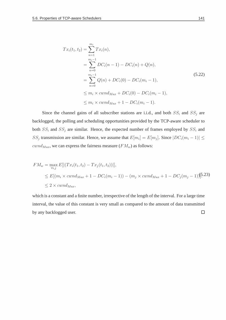
5.6. Properties of TCP-aware Schedulers 141
Txi(t1, t2) =
mi∑
n=1
Txi(n),
=
mi−1∑
n=0
DCi(n− 1) −DCi(n) +Q(n),
=
mi−1∑
n=0
Q(n) +DCi(0) −DCi(mi − 1),
≤ mi × cwndMax +DCi(0) −DCi(mi − 1),
≤ mi × cwndMax + 1 −DCi(mi − 1).
(5.22)
Since the channel gains of all subscriber stations are i.i.d., and bothSSi andSSj are
backlogged, the polling and scheduling opportunities provided by the TCP-aware scheduler to
bothSSi andSSj are similar. Hence, the expected number of frames employed by SSi and
SSj transmission are similar. Hence, we assume thatE[mi] = E[mj ]. Since|DCi(mi − 1)| ≤
cwndMax, we can express the fairness measure (FMw) as follows:
FMw = max∀i,j
E[|(Txi(t1, t2) − Txj(t1, t2))|],
≤ E[(mi × cwndMax + 1 −DCi(mi − 1)) − (mj × cwndMax + 1 −DCj(mj − 1))].
≤ 2 × cwndMax,
(5.23)
which is a constant and a finite number, irrespective of the length of the interval. For a large time
interval, the value of this constant is very small as compared to the amount of data transmitted
by any backlogged user.


Part II
Channel aware Congestion Control in
Infrastructure-less Ad-hoc Networks
143


Chapter 6
Congestion Control in Wireless Ad-hoc
Networks
We have discussed TCP-aware fair uplink scheduling schemesfor a multipoint-to-point network
in Chapters 4 and 5. These schemes operate at the MAC layer of the protocol stack and facilitate
the TCP-based applications to achieve higher throughput without altering the congestion control
mechanism of TCP. These are centralized uplink scheduling schemes and are cross-layer in
nature, involving PHY, MAC and Transport layers. However, these scheduling schemes are not
applicable in de-centralized wireless networks, such as wireless ad-hoc networks, as there is no
central entity involved for scheduling.
In ad-hoc networks, in addition to the location dependent time varying nature of wireless
channel, interference and limited energy of wireless nodesalso pose challenges in designing
schemes to provide higher throughput. For the best effort services, Transmission Control Pro-
tocol (TCP) based congestion control technique plays a significant role while designing these
systems. This is because, TCP treats packet drops as an indication of congestion. However,
in wireless networks packet drops can occur not only becauseof congestion in the network,
but also due to interference and wireless channel characteristics. This can be alleviated either
by: (1) modifying TCP congestion control mechanism, takingthe nature of wireless channel
and network model into consideration or by (2) exploring channel aware congestion control
mechanism. Since TCP is a popular protocol, modification of TCP to alleviate packet drops due
to interference and channel characteristics is not advisable. Instead, this can be alleviated by
channel aware congestion control techniques.
145

146 Chapter 6. Congestion Control in Wireless Ad-hoc Networks
This chapter is organized as follows. In section 6.1, we discuss various congestion con-
trol techniques used in wired networks. In Section 6.2, we model congestion control of wired
network using an optimization framework. We review the extension of congestion control tech-
niques proposed for wired network to wireless networks in Section 6.3. In Section 6.4, we
discuss the need of cross-layer congestion control technique, model an optimization-based con-
gestion control technique and discuss the nature of the utility function of TCP NewReno. We
discuss some of the open problems in cross-layer based congestion control in ad-hoc networks
in Section 6.5.
6.1 Congestion Control in Wired Networks
In Section 4.1, we have discussed TCP and its window evolution. In this section, we discuss
some congestion control techniques used in wired networks.This section presents a brief review
of published techniques and terminology, which we use in therest of the chapter. Comprehen-
sive account of congestion control techniques can be found in [42,43,72,76–78].
In a wired network, the links are assumed to be reliable and offixed capacities. There-
fore, any packet loss, delay or out of order delivery of packets is mainly due to congestion in
the network. Congestion in the network can be detected by theTCP of the protocol stack. To
counter congestion in the network, TCP retransmits lost packets, rearranges out-of-order deliv-
ered packets and adapts its rate of transmission by controlling its congestion window (cwnd)
size. Congestion control techniques of TCP can be broadly divided intoCongestion Controland
Congestion Avoidance. In congestion control [79], TCP controls thecwnd size as the network
parameterafter sensing congestion in the network (reactive); whereas, in congestion avoid-
ance, TCP controls thecwnd size as the network parameterbeforeit experiences congestion
(proactive). The congestion control techniques are further divided into three broad categories,
(i) window-based, (ii) equation-based, and (iii) rate-based, which are discussed in the following
sections.
6.1.1 Window-based Congestion Control
The congestion control algorithm followed by most of the variants of TCP is an end-to-end
window-based congestion control technique [72], which employs cwnd size as the network

6.1. Congestion Control in Wired Networks 147
parameter. These variants of TCP follow anAdaptive Window Managementtechnique in which
the sources increase theircwnd sizes on reception of successfulACK packets. Contrary to
that when the TCP sources receive multipleACKs of a same packet in succession or do not
receive anyACK before the expiry of a timeout, they decrease theircwnd sizes. In TCP,
instead of using linear increase and decrease ofcwnd, Additive Increase and Multiplicative
Decrease (AIMD) method is being used. Moreover, the manner of increase and decrease of
cwnd size is different for different TCP implementations. We discuss some of the commonly
used implementations as follows:
TCP Tahoe: In TCP Tahoe [80], congestion is detected by timeouts only.On timeouts, the
TCP source decreasescwnd size to one. This phase of TCP Tahoe is known asfast retransmit.
After it drops itscwnd size to one, it increases itscwnd size from one tossthresh (which acts
as limit point) in an exponential manner in eachRTT . This phase is known asslow start
phase. After reachingssthresh, the source increases itscwnd size linearly in eachRTT till it
experiences congestion. This phase is known ascongestion avoidancephase.
TCP Reno: In TCP Reno [73], congestion is detected by both tripledupacksand timeouts.
On timeouts it works similar to TCP Tahoe. However, with triple dupacks, it follows fast
recoverytechnique and decreases itscwnd value by half of its current size and then increases
linearly until it experiences congestion. Though it is better than TCP Tahoe for dealing with
single packet loss and tripledupacks, the performance suffers when multiple packets are lost
within oneRTT . This problem is addressed in its later version called NewReno or TCP Reno-2.
TCP NewReno: TCP NewReno (TCP Reno-2) [74, 81] is an extension of TCP Reno. It
follows exactly as TCP Reno except for the multiple packet drops in oneRTT . In NewReno,
cwnd value is not decremented for every packet loss, instead it isdecremented in an intelligent
manner. In this scheme, for multiple packet drops within oneRTT (multiple packet losses from
a single window of data), instead of dropping itscwnd size by multiple times, the TCP source
drops only once in thatRTT .
TCP Vegas: In TCP Vegas [82, 83], packet delay rather than packet loss is used as an
indication of congestion in the network. In this scheme, theTCP sources increase or decrease
theircwnd sizes based on the difference between the expected throughput (ratio of currentcwnd
size and the minimumRTT measured, which is known asbaseRTT) and actual throughput
(ratio of number of bytes transmitted during the lastRTT , known asrttLenand averagedRTT

148 Chapter 6. Congestion Control in Wireless Ad-hoc Networks
of the last segment). In this scheme, TCP sources decrease their cwnd sizes before experiencing
any congestion in the network in a more aggressive manner than Reno and Tahoe. TCP Vegas
is proactive, whereas TCP Tahoe, Reno and NewReno are reactive.
6.1.2 Equation-based Congestion Control
In window-based congestion control, the TCP sources adapt their cwnd sizes using AIMD
technique. However, adaptation ofcwnd sizes will have an impact on the performances when
the applications are played real-time. This is because, if the TCP sources drop theircwnd sizes
in a multiplicative manner (either by half of its current value or to one) on every congestion
indication they experience, then there will be abrupt changes on the send rate (transmission rate)
of the applications, which will have a noticeable impact on the performance of the application.
Instead, to maintain the quality of reception, one needs to maintain a relatively steady send rate,
while still being responsive to congestion. The equation-based congestion control [84] adapts
its send rate based on the loss event rate, which in turn depends upon the number of packets
dropped within a singleRTT . It uses a control equation that explicitly gives the maximum
acceptable send rate as a function of the recent loss event rate. Instead of reducing the rate of
transmission drastically using any AIMD technique, it reduces its rate of transmission guided
by a control equation. It increases its send rate in a slow rate, in response to a decrease in loss
event rate.
6.1.3 Rate-based Congestion Control
The analysis in [85], shows that the instantaneous throughput of a connection is inversely pro-
portional to the square of round-trip delay of the connection. The window-based congestion
control is unfair towards the connections with higher round-trip delays. When multiple con-
nections share a bottleneck link and the delay-bandwidth product is large, adapting the rate of
transmission using AIMD technique can lead to underutilization of bandwidth. Since the delay
of the network is very high, the sources will take long time toreach the available bandwidth.
Moreover, unfairness will result if flows have differentRTTs.
The unfairness and the underutilization of the network bandwidth can be alleviated, if the
delay-bandwidth product is lesser than the buffer in the link. In that case, the instantaneous
throughput or rate of transmission of an user can be approximated byxi = cwndi
RTTi, wherexi is

6.1. Congestion Control in Wired Networks 149
the instantaneous rate,cwndi is the window size andRTTi is theRTT of useri at that instant.
Hence, for a high speed network, the congestion control can be modeled as rate-based instead of
usual window-based one. Instead of changing the window sizein eachRTT , instantaneous rates
can be regulated at a smaller time scale to avoid congestion.By regulating the instantaneous
rates in this manner, maximum bandwidth can be utilized.
Rate-based congestion control scheme has been further investigated in [86]. In [86],
the authors formulate end-to-end congestion control as a global optimization problem of a
class of Minimum Cost Flow Control (MCFC) algorithms for controlling the rate of a con-
nection/session or window size. The window-based congestion control of TCP is shown as a
special case of MCFC algorithm in this paper.
Along with the above categories of congestion control schemes, Adaptive Queue Manage-
ment (AQM) based schemes are also employed to control congestion in the network. Schemes
like Random Early Detection (RED) [87] and its variants (Stabilized RED (SRED) [88], Adap-
tive RED (ARED) etc.) and Explicit Congestion Notification (ECN) [34] are also used to control
congestion in a proactive manner. In these schemes, along with the end-to-end principle of TCP,
network feedback is used for congestion detection. In the next section, we discuss ECN and its
use in brief.
6.1.4 Explicit Congestion Notification
It is a congestion avoidance technique where the sink indicates congestion before the on set
of actual congestion in the network. This is achieved by the AQM mechanism which allows
routers to set the Congestion Experienced (CE) code-point in a packet header as an indication
of congestion (instead of relying solely on packet drops). This has the potential of reducing
the impact of loss on delay-sensitive flows. This technique is known as Explicit Congestion
Notification (ECN) [34]. ECN for wired network is a well established technique. There are few
studies [89,90], which exploit the ECN marking of wired network to control the random losses
due to the time varying nature of wireless channel. But, these models do not consider losses due
to fading and they do not distinguish the packet losses due totime varying nature of the channel
and due to congestion in the network. Further studies are required in this direction such that
ECN can distinguish between wireless channel loss and congestion loss, and to model a flow
control problem of window size in wireless ad-hoc networks.This can improve the end-to-end

150 Chapter 6. Congestion Control in Wireless Ad-hoc Networks
throughput of wireless networks.
6.2 Congestion Control using Optimization Framework
Modelling congestion control as an optimization flow control problem has been addressed
in [33, 79, 91–93]. These articles have modelled congestioncontrol as a constraint based opti-
mization problem. Though all of them model congestion control problem as a social optimiza-
tion problem, each has a different solution approach. In this section, we discuss two specific
approaches such as,Charging and Rate Control[91] or Kelly’s ModelandOptimization Flow
Control [33] or Low and Lapsley Model, to solve the constraint based optimization problem and
the congestion in the network. Before discussing the solution methodologies, we explain the
system model in the following section.
6.2.1 System Model and Problem Formulation
We consider a network ofN communicating nodes connected byL links. The links are indexed
by l ∈ L and have finite capacitycl packets/sec. Let a set ofI source-sink pairs (flows) share
the network ofL unidirectional links. Let each source-sink pairi ∈ I be associated with a
transmission ratexi. Let Ui(xi) be the utility associated with the transmission ratexi. We
assume that the utility function is concave, increasing anddouble differentiable [94] for elastic1
traffic. LetH denote the routing matrix comprising of the route information of all possible
links. We assume stationary routing in our analysis. The elements of the routing matrixH are
expressed as:
Hli =
1 if, source-sink pairi uses linkl.,
0 otherwise.(6.1)
We define the aggregate flowyl (packets/sec) at linkl as:
yl =∑
i
Hlixi. (6.2)
1Elastic traffic consists of traffic for which users do not necessarily have a minimum requirements, but would
get as much as data through to their respective destinationsas quickly as possible [95].

6.2. Congestion Control using Optimization Framework 151
Let µl be the cost of transmission associated with linkl. The cost of transmissionµl can
be considered as the congestion cost of the link. The total cost associated with the source-sink
pair i is expressed as:
qi =∑
l
Hliµl. (6.3)
Both [91] and [33] consider the objective of maximizing the aggregate utility of all sources
(or system utility) subject to linear capacity constraintsof the links. This corresponds to a
system/social optimality and is expressed as:
maxxi≥0
∑
i
Ui(xi),
s. t.,∑
i∈I(l)
Hlixi ≤ cl;
X = {xi}, X ≥ 0.
(6.4)
Solving Eqn. (6.4) centrally would require the knowledge ofall utility functions and
coordination among all sources as the sources share the links. Since this is not possible in
practical networks, various de-centralized solutions have been considered. We discuss such
different de-centralized approaches in the subsequent sections.
6.2.2 Charging and Rate Control
In this model, a user (source-sink pair) chooses the charge per unit time that it can pay. The
network determines the rate at which the user should transmit according to a proportional fair-
ness criterion applied to the rate per unit charge. A system equilibrium is achieved when the
users choice of charges and networks choice of allocated rates are in equilibrium. The system
comprises both the users with utility functions and a network of links with capacity constraints.
As discussed in [91], the system optimization problemSY STEM(U,H,C) is identical to that
of Eqn. (6.4). Solution to the system optimization problem is obtained by solving two sub-
problems; one at the user level, known asUSER(Ui(xi), qi) and the other at the network level,
known asNETWORK(H,C; q). USER(Ui(xi), qi) is also known as user optimization prob-
lem, whereasNETWORK(H,C; q) is known as revenue optimization problem. These two
subproblems are expressed as:

152 Chapter 6. Congestion Control in Wireless Ad-hoc Networks
USER(Ui(xi), qi)
maxxi≥0
Ui(xi) − qixi, (6.5)
whereqi is the charge per unit flow that useri is willing to pay. The user is allowed to varyxi
freely.
NETWORK(H,C; q)
maxX≥0
∑
i
qixi,
s. t., HX ≤ C;
X = {xi} and C = {cl}
(6.6)
Since there exists a uniqueqi that solvesUSER(Ui(xi), qi) and at the same time, there
exists an optimalX = {xi} for the charge that the network receivedq = {qi} by solving
NETWORK(H,C; q), SY STEM(U,H,C) has a unique solution.
6.2.3 Optimization Flow Control
Solving Eqn. (6.4) not only requires the knowledge of utility function of all users, but also
requires coordination of all users. Since in a de-centralized network, obtaining the knowledge
of the utility function of all users and coordination among all users is not possible, [33] proposes
de-centralized solution to determine the source ratexi of each users. This solution is a reactive
flow control technique, where each linkl ∈ L determines a priceµl for a unit bandwidth inl,
based on all local source ratexi at that link. A sourcei ∈ I is fed back with the total price
in its pathqi =∑
l∈LHliµl, which we illustrate in Figure 6.1. Therefore, the individual profit
maximization of a sourcei becomes:
maxxi
[
Ui(xi) − qixi
]
,
xi ≥ 0.
(6.7)
By solving Eqn. (6.7), each user obtains the optimal transmission ratexi and achieves
maximum profit. All sources determine their transmission rates in an adaptive manner as per
the network load in each iteration. The individual optimal rates thus obtained may not lead to a
social optimal solution (Eqn. (6.4)) for a general price vector µ = {µl}, l ∈ L. Instead, [33]
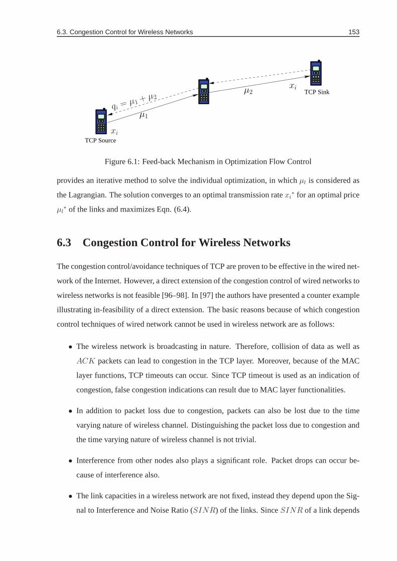
6.3. Congestion Control for Wireless Networks 153
TCP Sink
TCP Source
xi
xi
qi = µ1 + µ2
µ1
µ2
Figure 6.1: Feed-back Mechanism in Optimization Flow Control
provides an iterative method to solve the individual optimization, in whichµl is considered as
the Lagrangian. The solution converges to an optimal transmission ratexi∗ for an optimal price
µl∗ of the links and maximizes Eqn. (6.4).
6.3 Congestion Control for Wireless Networks
The congestion control/avoidance techniques of TCP are proven to be effective in the wired net-
work of the Internet. However, a direct extension of the congestion control of wired networks to
wireless networks is not feasible [96–98]. In [97] the authors have presented a counter example
illustrating in-feasibility of a direct extension. The basic reasons because of which congestion
control techniques of wired network cannot be used in wireless network are as follows:
• The wireless network is broadcasting in nature. Therefore,collision of data as well as
ACK packets can lead to congestion in the TCP layer. Moreover, because of the MAC
layer functions, TCP timeouts can occur. Since TCP timeout is used as an indication of
congestion, false congestion indications can result due toMAC layer functionalities.
• In addition to packet loss due to congestion, packets can also be lost due to the time
varying nature of wireless channel. Distinguishing the packet loss due to congestion and
the time varying nature of wireless channel is not trivial.
• Interference from other nodes also plays a significant role.Packet drops can occur be-
cause of interference also.
• The link capacities in a wireless network are not fixed, instead they depend upon the Sig-
nal to Interference and Noise Ratio (SINR) of the links. SinceSINR of a link depends

154 Chapter 6. Congestion Control in Wireless Ad-hoc Networks
upon the power transmission policy of the network, packet loss at a link is affected by the
power transmission policy of the network
Hence, applying the congestion control of wired networks directly in wireless networks
may underestimate the capacity of the networks, leading to non-optimal performance and un-
derutilization of resources.
There are various methods that have been proposed to solve the congestion control prob-
lem in wireless networks. These can be broadly divided into two categories: (1) Modification of
TCP congestion control mechanism, taking the nature of wireless channel and network model
into consideration; and (2) Changing the PHY and MAC layer functionalities based on the
TCP’s requirement. In the former approach, various new TCP congestion control techniques
such as Split TCP [99], Ad-hoc TCP (ATCP) [100], TCP-BuS [101] and TCP-snoop [102] have
been proposed in the literature. In the later approach, there are also few proposals, such as joint
congestion and power control in wireless networks [30], joint scheduling and congestion con-
trol [103] and joint routing, scheduling and congestion control [104] that have been proposed in
the literature. In this thesis, we concentrate on the secondapproach, i.e., we propose methods
to improve TCP performances by exploiting PHY and MAC layer functionalities, discussed in
detail in the next chapter.
As suggested before, there is a need of modification of the utility-based optimization
framework for congestion control to accommodate the time varying channel and interference of
neighboring nodes. Moreover, in a multi-hop wireless network, battery power of wireless nodes
should also be considered in the optimization process, which is not addressed in any of these
papers so far. We discuss these issues in the following sections.
6.3.1 Towards an Optimization Framework for Congestion Control in
Wireless Networks
Various authors have studied the congestion control techniques of TCP in a wireless network.
[30–32] have used power control along with congestion control in a wireless network and have
analyzed it for TCP Vegas. In [105], the author has modeled the joint power control and utility
maximization of a wireless network as a sum product problem.This approach is used to de-
sign a new Joint Optimal Congestion control and Power control (JOCP) algorithm (for a wire-
less network). [105] proposes a distributed power control algorithm which works jointly with

6.4. Cross-layer Congestion Control in Wireless Networks 155
the existing TCP congestion control algorithm in order to increase the end-to-end throughput
and energy efficiency of a multi-hop wireless network. This JOCP algorithm does not change
the original TCP and layered structure of the network. Instead, it is a cross-layer approach,
where the interactions among the Physical and Transport layer is used to increase the end-to-
end throughput.
6.4 Cross-layer Congestion Control in Wireless Networks
In this section, we discuss a cross-layer congestion control technique based on sum product
algorithms of [105] for TCP NewReno in a wireless network. Since in wireless networks,
multiple packets can drop due to congestion as well as due to the time varying nature of the
channel in oneRTT , use of TCP NewReno is more appropriate. This is because, thevalue of
cwnd does not get decremented for more than half of its current value if multiple packet of a
single window of data are lost in oneRTT , which is common in wireless networks. Therefore,
in TCP NewReno, packet loss due to wireless channel is also being taken care of. We consider
the following steps to achieve a cross-layer congestion control algorithm for TCP NewReno in
this thesis.
1. Formulation of TCP congestion control in terms of controlsystem equations.
2. Use of optimization techniques to determine the maximum aggregate utility of sources,
subject to capacity constraints and maximum transmission power [91] of wireless nodes.
6.4.1 System Model
The system model we use in this section is an extension of the system model illustrated in
Section 6.2. We consider a network ofN communicating nodes connected byL communicating
links that are shared byI source-sink pairs. We illustrate this with an example through Figure
6.2. It is a small topology with six nodes, five links and two pairs of source-sink pairs or flows
(between node 1 and node 5 and node 2 and node 6). Routing matrix H consists of the routing
elements of the network.
For analyzing TCP congestion control, we consider a feedback system model which con-
sists of a Source Controller and a Link Controller as shown inFigure 6.3. The input to the source

156 Chapter 6. Congestion Control in Wireless Ad-hoc Networks
2 5
3
1
4
6Flow 1
Flow 2
Figure 6.2: System Model/Topology
controller is the change in cost (∆q) of all I source-sink pairs and the output of the source con-
troller is the change in rate of transmission (∆x) of all source-sink pairs. This is equivalent
to solving theUSER(Ui(xi), qi) in Section 6.2.2. Similarly, the input to the link controller
is the change in aggregate traffic in each link (∆y) and the output of the link controller is the
individual link costµl of each linkl. This is equivalent to solvingNETWORK(H,C; q) in
Section 6.2.2. The nodal pointsF1 andF2 determine the change in aggregate traffic in each
link and aggregate price of each source-sink pair respectively. Though, there are time delays
associated with the function of each block of the source-sink controller, we do not reflect that
in our analysis for simplification. However, we incorporatethe total delay as the Round Trip
Delay, i.e.,RTTi = RTT fi + RTT bi , whereRTT fi is forward delay (in practice the delay of a
data packet from the source to sink) andRTT bi is the backward delay (in practice the delay of
anACK packet from the sink to source).
6.4.2 Problem Formulation
We formulate our problem statement initially for a wired network, similar to [106, 107] and
then extend it to a wireless network. Our system model is based on fluid-flow abstraction. We
consider long TCP connections instead of short ones in our model, as the former corresponds to
majority of the TCP traffic in the Internet. We use control system equations [107] to determine
the equilibrium point (x∗, y∗, q∗) for our system with the following assumptions: (1) resource
allocation is characterized by a demand curvex∗i = fi(q∗i ), (2) aggregate flow is less than or
equal to the capacity of the link, i.e.,y∗l ≤ cl, and (3) the equilibrium queues are either empty

6.4. Cross-layer Congestion Control in Wireless Networks 157
Controller
F2
F1
SourceController
Link
∆y∆x
∆q ∆µ
Figure 6.3: Feedback System Model
or small enough to avoid the queuing delays. The demand curvespecified above is a decreasing
function of price, which is equivalent to the use of an utility functionUi(xi) defined by [94],
which is concave and continuously differentiable functionof xi for xi ≥ 0, i.e. fi = (U′
i )−1
. At
equilibrium, a source chooses its maximum profit by solving it as:
maxx∗i
[
Ui(x∗i ) − q∗i x
∗i
]
, (6.8)
whereq∗ = HTµ∗, andx∗, y∗, q∗ are the optimal fixed parameters. Since at equilibrium, each
source attempts to maximize its profit (individual optimality) by choosing an appropriate rate;
the individual optimality of Eqn. (6.8) can be re-written asa social optimality equation [78]:
maxX≥0
∑
i
Ui(xi),
s. t., HX ≤ C;
X = {xi} and C = {cl}
(6.9)
Using Karush-Kuhn-Tucker (KKT) condition on the social optimal equation (Eqn. (6.9))
as in [106], the constrained global maxima point2 X∗ = {x∗i } is expressed as:
∇∑
i
U(xi) −∑
l
µl∇(HX) = 0; ∀µl > 0, (6.10)
2Since the utility functionU(xi) is concave and increasing, KKT conditions are necessary andsufficient for a
global maximum.

158 Chapter 6. Congestion Control in Wireless Ad-hoc Networks
whereµl is the Lagrangian Multiplier and is used as link prices (shadow prices) as discussed
in [91] and [108]. Hence, Eqn. (6.10) is reduced toU′
i (xi) = q∗i at the global maximum
point. The primal-dual distributed algorithm of the maximization equation Eqn. (6.9) signifies
that the price is updated as a congestion parameter and is a dual variable. We now extend the
optimization based congestion control technique to wireless network in the following section.
6.4.3 Extension to Wireless Networks
As discussed in [30], price is considered as a function of transmit power. By appropriate power
control of all nodes, the maximum aggregate throughput can be attained. However, the increase
of power in one node has a direct effect on the data rates of other nodes due to interference.
Hence, we modify the maximization equation (Eqn. (6.9)) as follows:
maxX≥0
∑
i
Ui(xi),
s.t., HX ≤ C(P ); P = {Pl},
Pl ≤ PlMax, ∀l,
P,X ≥ 0,
(6.11)
wherePl is the transmission power of a node inlth link. Here, the link capacitycl is a function
of transmission powerPl in that link. Since it is observed in [109, 110] that power control
significantly increases throughput in both CDMA and non-CDMA wireless networks, we use
power control mechanism to achieve congestion control by the above optimization techniques.
This is a cross-layer power and congestion control technique.
As discussed before, different variants of TCP have different utility functions. Since we
use TCP NewReno, we now study the utility function of TCP NewReno and its properties.
6.4.4 Utility Function of a Practical Congestion Control Algorithm
In TCP NewReno,cwnd is decreased by half for one or more congestion notification or triple
dupacks or incremented by one for no mark in oneRTT . We assume the marking probability
to be a measure of congestion [106]. Ifτi is the equilibriumRTT (assumed to be constant for
all), then transmission ratexi(t) of a source-sink pairi ∈ I is expressed as:

6.4. Cross-layer Congestion Control in Wireless Networks 159
xi(t) =cwndi(t)
τi, (6.12)
wherecwndi(t) is the window size at time instantt. The transmission ratexi(t) is interpreted as
the average rate overt. If there is no mark in oneRTT (τi), then,cwndi(t+τi) = cwndi(t)+1,
else,cwndi(t + τi) = cwndi(t)/2, for one or more mark in oneRTT . Hence, the increase in
window size is1/τi with probability (1− pi(t)) and the decrease is by2cwndi(t)3τi
3 with probability
pi(t). pi(t) is the end-to-end probability that at least one packet is marked out of all packets of
an window, in a periodt for the source-sink pairi (the packet marking are independent). We
approximate [106]pi(t) for smallqi(t) (aggregate price of all links in the route Eqn. (6.3)) as
follows:
pi(t) = 1 − (1 − qi(t))cwndi(t) ≈ cwndi(t)qi(t) (6.13)
Thus, the average change in window size4 in the periodt is:
xi(t) =1
τi
(
1 − pi(t)
)
−2
3
cwndi(t)
τipi(t) (6.14)
From Eqn. (6.13) and Eqn. (6.14), we determine the equilibrium parameters as follows:
x =xi(t)
τi=
1 − cwndi(t)qi(t)
τ 2i
−2
3τiqi(t)xi(t)cwndi(t) (6.15)
At equilibrium, settingx = 0, xi(t) = x∗i andqi(t) = q∗i in Eqn. (6.15), we determineq∗i :
q∗i =3
xi(t)τi(3 + 2xi(t)τi). (6.16)
Now, using the fact thatU′
i (xi) = q∗i , the utility function is expressed as:
Ui(xi) =
∫
q∗i dxi =1
τilog
[xiτi
2xiτi + 3
]
. (6.17)
Since the utility function of TCP NewReno, derived above, isconcave forxi, τi ≥ 0, our
problem formulation in Eqn. (6.8) holds good.
3For a single NewReno flow, the window oscillates between4cwndi(t)3τi
and 2cwndi(t)3τi
with an average of
cwndi(t) [106].4The change in window size due to time-out is neglected here.

160 Chapter 6. Congestion Control in Wireless Ad-hoc Networks
6.5 Discussions on Open Problems
In the recent years, there has been an explosion of research in cross-layer congestion control
techniques with the prime motive of higher TCP throughput. There are some attempts, which
have addressed on a cross-layer congestion and power control in wireless networks. However,
practical implementations of cross-layer congestion and power control in real life network has
not been explored properly. In addition, life time of the network, energy constraints of the
wireless nodes and energy cost of the wireless nodes have also not been considered fully. The
implementation methodologies, convergence analysis and effect of short flows on cross-layer
congestion control and power control have also not been discussed in details [30–32].
In this direction, we attempt to solve some of these problemsin this thesis. We attempt to
propose a channel aware congestion and power control technique for a CDMA ad-hoc network,
in which both congestion cost and energy cost are considered. We aim to minimize the energy
spent for transmission and thereby increase the life-time of the network. Using, exhaustive sim-
ulations we show improvements in TCP throughput and convergence of the proposed algorithm.
We also suggest implementation methodologies using ECN framework. We discuss the details
of these problems in the next chapter.

Chapter 7
Joint Congestion and Power Control in
CDMA Ad-hoc Networks
In the previous chapter, we have modelled TCP congestion control in wireless ad-hoc networks
as a social optimization problem and employ congestion in a link as a cost function. Since
the wireless nodes are mostly battery powered, the transmission power in a link should also be
considered as a cost function. However, inclusion of cost function for transmission power in
a link may lead to convergence problem. Therefore, further investigation on cross-layer based
congestion and power control in ad-hoc networks is required. In addition, implementation of
the cross-layer based congestion control in the protocol stack requires further investigation.
To address the above mentioned issues, in this chapter, we consider CDMA ad-hoc networks
as an example and propose a joint congestion and power control scheme in ad-hoc networks,
which employs both congestion and energy cost. We model TCP congestion control in wireless
networks as a social optimization problem and decompose theobjective function defined for
social optimization in wireless ad-hoc networks into two separate objective functions [32]. We
solve these separate objective functions iteratively for the equilibrium transmission rates and
link costs (both congestion cost and energy cost). The solution of the decomposed objective
functions leads to a cross-layer approach involving TCP andthe PHY layer, in which power
transmission in a link is determined based on the interference and congestion in the network
and the rate of transmission is determined based on congestion in the network. Note that we do
not modify TCP congestion control protocol, instead we control the transmission power in an
optimal manner to achieve higher throughput. We also propose an implementation method for
161

162 Chapter 7. Joint Congestion and Power Control in CDMA Ad-hoc Networks
the cross-layer congestion control scheme using Explicit Congestion Notification (ECN) [34].
This chapter is organized as follows. In Section 7.1, we formulate a joint congestion and
power control problem for a CDMA ad-hoc network. In Section 7.2, we discuss congestion cost,
energy cost and attempt to solve the optimization problem inan iterative way. To determine the
efficiency of our framework, we describe the experimental evaluation and discuss the results of
our simulations in Section 7.3. In Section 7.3, we also investigate the convergence nature of the
proposed scheme analytically and through simulations. We describe an implementation method
of the cross-layer congestion control scheme using Explicit Congestion Notification (ECN) in
Section 7.5.
7.1 System Model and Problem Formulation
The system model we use in this section is an extension of the system model illustrated in
Section 6.2. We consider a CDMA ad-hoc network ofN communicating nodes connected by
L unidirectional communicating links and shared byI source-sink pairs. In the CDMA ad-hoc
network every participating node has the capability to transmit at different power levels as per
its requirements and transmits with different CDMA codes. Let each link be indexed byl and
let cl(Pl) denote the capacity of linkl ∈ L, wherePl is the transmission power on the linkl.
Note that the capacity of each link defined in Section 6.2 is fixed, whereas it is time varying in
this section. LetSINRl be the Signal-to-Interference-and-Noise Ratio of linkl ∈ L.
SINRl =PlGll
∑
k 6=l PkGlk + nl, (7.1)
whereGll is the path gain from the transmitter of linkl to the receiver of the linkl andGlk is
the path gain from the transmitter on linkk to the receiver on linkl. nl is the thermal noise on
the link l. We can determine the maximum capacity attainable in linkl as:
cl(Pl) = B × log(1 +MI × SINRl) packets/sec, (7.2)
whereB is the channel bandwidth andMI is a constant that depends on the modulation scheme
used by the node for a successful transmission.
Let each source-sink pairi ∈ I be associated with a transmission ratexi andUi(xi) be the
utility associated with the transmisson ratexi. Let the routing matrixH consist of the routing

7.1. System Model and Problem Formulation 163
elements of the network. The elements of the routing matrix are either “1” or “0”, as explained
in Eqn. (6.1). The aggregate flowyl (packets/sec) at linkl is defined in Eqn. (6.2) and the total
costqi associated with a source-sink pairi is defined in Eqn. (6.3). We now attempt to solve the
social optimization problem described in Eqn. (6.11), which we reproduce below (Eqn. (7.3))
for completeness.
maxX≥0
∑
i
Ui(xi),
s.t., HX ≤ C(P ); P = {Pl},
Pl ≤ PlMax, ∀l,
P,X ≥ 0,
(7.3)
wherePlMaxis the maximum power that a node can transmit. Since the utility function is
concave and double differentiable and the constraints are linear, we can associate a Lagrangian
Multiplier µl with the first constraint of Eqn. (7.3). The Lagrangian Multiplier µl can also
be interpreted as the network cost or shadow price of transmission in the link. We now use
KKT [111] optimality conditions to determine the stationary points (X∗ = {x∗i } andµ∗ = {µ∗l })
by solving the complementary slackness conditions at equilibrium, i.e.,
φsystem(X,P, µ) =∑
i
Ui(xi) −∑
l
µl(∑
i
Hlixi − cl(P )). (7.4)
Maximization ofφsystem in Eqn. (7.4) is decomposed1 as in [30]:
max I(X,µ) =∑
i
Ui(xi) −∑
l
µl∑
i
Hlixi,
max I(P, µ) =∑
l
µlcl(P ),
s.t., X ≥ 0; 0 ≤ Pl ≤ PlMax.
(7.5)
Both I(X,µ) andI(P, µ) are related by a common variableµ, which plays a significant
role in determining the equilibrium window size (hence the data rate) and transmission power.
Any change inµ results in change in throughput and transmission power. Thefirst maximization
1Distributed solution is possible as long as there is an interaction between the two decomposed equations
through some information passing. This is known as sum product algorithm [105].

164 Chapter 7. Joint Congestion and Power Control in CDMA Ad-hoc Networks
equation involvingI(X,µ) in Eqn. (7.5) is a direct consequence of congestion control of TCP.
It is solved by the congestion control mechanism of TCP by increasing/decreasing thecwnd
size (and hence the individual data rates) for each flow in every RTT . Since the utility function
of TCP NewReno(Ui(xi) = 1
τilog[
xiτi2xiτi+3
])is concave and twice differentiable forxi, τi ≥ 0,
I(X,µ) will converge to a global maximum.
The second maximization equation involvingI(P, µ) in Eqn. (7.5) is solved by choosing
appropriate transmission power of wireless nodes. Before investigating the nature ofI(P, µ),
we discuss the nature of shadow priceµl of a link. Since we consider both congestion cost and
the cost of transmission, i.e., energy cost, the shadow priceµl (and the Lagrangian Multiplier)
can be expressed as:
µl = λl, if “energy cost” is zero,
= λl + bl, otherwise,(7.6)
whereλl is the “congestion cost” andbl is the “energy cost” of the linkl. Before solvingI(P, µ),
we investigate the properties of the congestion cost and energy cost in the following section.
7.2 Solution Methodologies
As discussed earlier, we need to solve the sub-optimizationproblemI(P, µ) of Eqn. (7.5),
such that the social optimization defined in Eqn. (7.3) is solved. In the following sections, we
investigate the properties of both congestion cost and energy cost in detail.
7.2.1 Congestion Cost in TCP NewReno
We considerλl as the congestion cost of a linkl. Since packet drop is used as an indication
of congestion in TCP NewReno, probability of packet drop is used as congestion cost2. In this
section, we derive a closed form expression for the congestion cost of a link in TCP NewReno.
We assume that the packets traversing in linkl gets dropped if the aggregate traffic is more
than the link capacitycl. The probability of packet drop in a link can be modeled as packet loss
probability in aM/M/1/Z queue [90], where,Z is the buffer size at the link. In this kind of
2Concept of congestion cost is different for different versions of TCP. In TCP Vegas, queuing delay is used as
an indication of congestion and hence the congestion cost.

7.2. Solution Methodologies 165
queuing model,yl andcl serves as average arrival rate and average service rate3 respectively.
The loss probability (pl) for this kind of queue at equilibrium is defined as [112]:
pl(cl, yl) =(1 − ρ)ρZ
(1 − ρZ+1), (7.7)
whereρ := yl
cl. By scaling the arrival rate, departure rate and buffer capacity by a factorK as in
a many-source large-deviation scaling and by takingK → ∞, we determine the loss probability
as:
limK→∞
pl(cl, yl) = limK→∞
(1 − ρ)ρKZ
1 − ρKZ+1
= limK→∞
[
1 −1 − ρKZ
1 − ρKZ+1
]
=(yl − cl)
+
yl=
max(0, (yl − cl)
)
yl.
(7.8)
The above equation is valid only foryl > 0. Whenyl = 0, pl(cl, yl) = 0. Since the loss
probability (pl) in TCP NewReno is considered as the shadow price/cost, congestion costλl is
expressed as:
λl(t) = pl(cl(t), yl(t)) =
max(0,(yl(t)−cl(t))
)
yl(t)if yl(t) > 0,
0 if yl(t) = 0.
(7.9)
Since wireless channel as well as aggregate traffic in a link is time varying, we have
introduced the time instant “t” in the above equation, i.e., the congestion cost is also time
varying.
7.2.2 Energy Cost With and Without Battery Life Time
The energy cost is the cost of power spent by a wireless node totransmit its own traffic or to
rely (forward) others’ traffic. Energy cost is important when the nodes are battery powered and
maximum node life time is desired. The energy cost “bl” is a function of transmission powerPl
(i.e., energy consumption) of the node in that link.
3The maximum capacity of the link iscl and hence the service rate.

166 Chapter 7. Joint Congestion and Power Control in CDMA Ad-hoc Networks
For successfully delivering a packet there is a requirementof minimum Bit Error Rate
(BER) at the receiver. The minimumBER can be translated to a minimumSINR in the
link. In wireless link, theSINR in one link depends not only on the transmission power in the
same link, but also on the transmission power of other links.To maintain minimumSINR in
a desired link, the transmitting node needs to determine thePl required for that link (which is
affected by other’s transmission also). We now define a linear pricing equation for the energy
cost. Similar to the congestion cost, the energy cost is alsotime varying. We define the energy
cost as:
bl(t) = θ + α1f1(α2Pl(t)), (7.10)
whereθ is the minimum cost to keep the transmitter in “on” state (same asPlMin, the minimum
power transmission) andα1 andα2 are constants which can be chosen for a pricing model
by the network operator. The value ofα1 andα2 also indicate whether energy cost or the
congestion cost is dominant. The functionf1 is a piecewise monotonically increasing function.
In Eqn. (7.10), we have not considered the battery life time/life time of the network, which
is an important parameter. As the time progresses, the life time of a battery decreases, and
hence choosing a path through this node becomes a costly affair. Therefore, the life time of the
network should be reflected in the energy cost determination. We consider the energy cost as
a function of amount of energy spent and the life time available for the battery of a particular
wireless node. The energy cost on a path increases as the lifetime decreases. We consider a
non-linear pricing model for the energy cost with battery life time as follows:
bl(t) = θ + α1f1(α2Pl(t)) + α3f2(α4(Pavl −
t∑
t=0
Pl(t))) (7.11)
The third sum term of Eqn. (7.11) decides the cost due to the amount of battery available
in the wireless node.Pavl is the amount of energy available at the node before the startof the
operation andα3, α4 are some constants. Similar tof1, functionf2 can be any linear monotonic
increasing function. The operator or the node can choose this function in an appropriate manner.
In this chapter we use energy cost without battery life time for simplicity.

7.2. Solution Methodologies 167
7.2.3 Nature ofI(P, µ) and Solution to the Optimization Problem
With Congestion Cost only
We first consider the congestion cost only, i.e.,µl(t) = λl(t) and solveI(P, µ) as follows.
Without loss of generality, we assume that the bandwidthB and the modulation indexMI of
Eqn. (7.2) as unity and re-writeI(P, µ) as follows:
I(P, µ) = I(P, λ)
=∑
l
λllog(SINRl(P )).(7.12)
SinceI(P, µ) is a concave function of a logarithmic transformed power vector, Eqn. (7.4)
will converge to a global maxima resulting in optimumX∗ = {x∗i }, µ∗ = {µ∗l }. Solution of
I(P, µ) can be obtained as follows:
I(P, µ) =∑
l
µllog
(PlGll
∑
k 6=l PkGlk + nl
)
=∑
l
µl
[
log(Pl) + log(Gll) − log
(∑
k 6=l
PkGlk + nl
)] (7.13)
Next, by differentiatingI(P, µ) with respect toPl, we evaluate thelth component of the
gradient∇I(P, µ).
∇I(P, µ) =µl(t)
Pl−∑
j 6=l
µj(t)Gjl∑
k 6=j PkGjk + nj(7.14)
Now, we use the Steepest Descent method as in [111] to solve the maximization problem
as:
Pl(t+ 1) = Pl(t) + δ
(
∇I(P, µ)
)
= Pl(t) + δ
(µl(t)
Pl(t)−∑
j 6=l
µj(t)Gjl∑
k 6=j Pk(t)Gjk + nj
)
= Pl(t) + δµl(t)
Pl(t)− δ
∑
j 6=l
mj(t)Gjl,
(7.15)
whereδ is a constant, called the step size in the direction of the gradient andmj(t) =µj(t)SINRj (t)
Pj(t)Gjj.
mj(t) can be interpreted as the interference received from nodej.

168 Chapter 7. Joint Congestion and Power Control in CDMA Ad-hoc Networks
In practice, power transmissionPl(t) is always bounded by the minimum power level
PlMinandPlMax
. Since the time scale of change ofcwnd is oneRTT , the time scale of the
change of transmission powerPl is also oneRTT . From Eqn. (7.15), it is evident that the
transmission power of a node in the next time instantPl(t + 1) in a link l depends on three
parameters, namely; (i) transmission power in the present time instantPl(t), (ii) shadow price
µ(t), and (iii) the weighted sum of interference received from all neighboring nodes. The third
factor is responsible for decreasing the transmission power of the concerned node in the next
time instant. This is known as the co-operation principle inpower control of wireless network.
Increase inµl(t) is responsible for increasing power in the next time instant. Intuitively, more
the shadow loss, more the congestion, thereby increasing the transmission power in the next
time instant.
With Congestion Cost and Energy Cost
We now consider both congestion cost as well as energy cost (without battery life time) to solve
I(P, µ). We re-writeI(P, µ) with both congestion and energy cost as follows:
I(P, µ) =∑
l
µllog(SINRl(P ))
=∑
l
(λl + bl)log(SINRl(P )).(7.16)
Instead of investigating the concave nature ofI(P, µ), we transform the power vectorP
to a logarithmic power vectorP and then investigate the concave nature of the transformed
I(P , µ). Let Pl = logPl, ∀l. We writeI(P , µ) as follows:
I(P , µ) =∑
l
µllog
[Glle
Pl
∑
k 6=lGlkePk + nl
]
=∑
l
λl
[
log(Gllepl) − log
(∑
k 6=l
ePl+logGlk + nl
)]
︸ ︷︷ ︸
I1(P ,µ)
+∑
l
bl
[
log(Gllepl) − log
(∑
k 6=l
ePl+logGlk + nl
)]
︸ ︷︷ ︸
I2(P ,µ)
= I1(P , µ) + I2(P , µ)
(7.17)

7.2. Solution Methodologies 169
From Eqn. (7.17), it is evident thatI1(P , µ) is concave inP , aslog(GllePl) is linear inP
andlog
(∑
k ePl+logGlk + nl
)
is convex inP .
I2(P , µ) =∑
l
θ
[
log(Gllepl) − log
(∑
k 6=l
ePl+logGlk + nl
)]
+∑
l
α1f1(α2Pl)
[
log(Gllepl)
− log
(∑
k 6=l
ePl+logGlk + nl
)]
(7.18)
Similarly, from Eqn. (7.18), it is evident thatI2(P , µ) is concave asf1(α2Pl) is linear
and monotonic inPl. Hence,I(P , µ) is concave inP and inP . SinceI(X,µ) andI(P, µ)
are concave and double differentiable, Eqn. (7.4) will converge to a global maxima resulting in
optimumX∗ = {x∗i }, µ∗ = {µ∗l }. The solution methodologies to find the global maxima are
explained below.
Each source-sink pairi solves the first maximization equation involvingI(X,µ) as it
knows its own utility functionUi(xi) and the end-to-end cost (which is fed back by the system)
by using TCP NewReno congestion control in every RTT. We solve the second maximization
equation involvingI(P, µ) by choosing appropriate transmission powers of the wireless nodes
as discussed below. DifferentiatingI(P, µ) with respect toPl, we evaluate thelth component of
the gradient∇I(P, µ). We use the Steepest Descent method to solve the maximization problem
with a small step sizeδ to obtain the transmission power as:
Pl(t+ 1) = Pl(t) + δ
(
∇I(P, µ)
)
. (7.19)
As discussed earlier, the time scale of change of transmission power is oneRTT . Each
node determines its required transmission powerPl (in practice the transmission power of a
node is bounded by minimum and maximum power levels) and network costµl of each outgoing
link associated with it and passes on these information to its neighbors, such that end-to-end cost
of a path can be determined by each source-sink pairi. Each source-sink pairi determines its
transmission rate using TCP NewReno and transmission powerusing Eqn. (7.19), which is
equivalent to solving a joint congestion control and power control for an ad-hoc network. It
is a channel aware congestion control technique. We suggestan algorithm to implement this
joint congestion and power control in Algorithm 4. The parameter∆ in Algorithm 4 is a small

170 Chapter 7. Joint Congestion and Power Control in CDMA Ad-hoc Networks
tunable system parameter. The value of∆ is set as the granularity of increase/decrease of power
level of a node.
In power control techniques, each wireless node needs to advertise itsSINRl requirement
either on a separate channel [110] or on the same channel [113]. These nodes update their path
gains, noise levels, interference caused by other nodes either after receiving the advertised signal
or in a periodic manner.
Algorithm 4 :Channel aware Congestion Control for CDMA Ad-hoc Network with Congestion
and Energy Cost1: cwndi(0)← 3 ∀i
2: Pl(0)← PlMax∀l
3: cl(0)← clMax∀l
4: bl(0)← θ ∀l
5: λl(0)← 0 ∀l
6: µl(0)← θ ∀l
7: t← 1
8: while TRUE do
9: UpdateGll andGlk periodically
10: SINRl(t)←Pl(t−1)Gll
P
k 6=l Pk(t−1)Glk+nl∀l
11: Pl(t)← Pl(t − 1) + δ(∇I(P, µ)) ∀l
12: if |Pl(t) − Pl(t − 1)| ≤ ∆ then
13: Pl(t)← Pl(t− 1) ∀l
14: else
15: Pl(t)← min(Pl(t), PlMax) ∀l
16: end if
17: Updatecwndi(t), τi from TCP Module∀i
18: xi(t)←cwndi(t)
τi∀i
19: yl(t)←P
i Hlixi ∀l
20: bl(t)← θ + α1f1(α2Pl(t)) ∀l
21: cl(t)←1T
log(1 +MI × SINRl(t)) ∀l
22: λl(t)←max(0,yl(t)−cl(t))
yl(t)∀l
23: µl(t)← λl(t) + bl(t) ∀l
24: qi(t)←P
l Hliµl ∀i
25: t← t + 1
26: end while
7.3 Experimental Evaluation of Channel aware Congestion
Control Algorithm
In this section, we describe simulation experiments that have been performed to evaluate chan-
nel aware congestion control algorithm. All the simulations have been conducted using im-

7.3. Experimental Evaluation of Channel aware Congestion Control Algorithm 171
plementations of cross-layer congestion control algorithm in MATLAB [68]. We consider a
CDMA ad-hoc network with six wireless nodes and two pairs of TCP source-sink pairs (1-5)
and (2-6) as in shown in Figure 7.1 (same topology is used hereas shown Figure 6.2). All
nodes in our simulation are capable of transmitting and receiving “network cost”. We also
consider that all six nodes are TCP NewReno agents. Depending upon the network costs,
we update the transmission power of the participating nodes. We set the TCP retransmission
timeout to be4 × RTT . We updateRTT by using the exponential averaging technique as:
RTT = ΥRTTestimated + (1−Υ)RTTmeasured. We assume thatΥ = 0.85 for our simulations.
We assume fixed packet lengths of 1000 bits size. We assume that the time required for trans-
mission in each of the segments (Figure 7.1) 1-3, 2-3, 3-4, 4-5 and 4-6 are same. We conduct
three different sets of experiments. They are: (i) Channel aware Congestion control with Con-
gestion Cost (CC-CC), (ii) Channel aware Congestion control with Network Cost (CC-NC) and
(iii) congestion control Without Power Control (W-PC) (congestion control with fixed power
transmissions)
The path loss exponent due to distance is set asγ = 4. We consider AWGN with PSDN0 =
0.35 (4.5 dB/Hz). We also simulate shadowing in our experiments. The shadowing is modeled
as Log-normal with mean zero and standard deviation (σ) 8 dB. In each simulation run, the
channel gain due to Log-normal shadowing is kept fixed for theentire duration of simulation.
We also repeat the experiments with different Log-normal shadowing withσ of 4, 6, 8, 10 and
12 dB. We assume channel reciprocity, i.e., both forward andreverse link gains are the same.
We implement TCP NewReno in MATLAB. We setcwndinitial = 3 packets,PlMin= 3
mwatt andPlMax= 10 mwatt in our simulations. We determine the data ratexi by using the
relationxi(t) = cwndi(t)τi
, whereascwndi(t) andτi are updated using TCP NewReno conges-
tion control principle. We also consider different step size (δ = 0.1, 0.2 and 0.5) to verify
the robustness and convergence of our algorithm. The systemparameters used for simulations
are presented in Table 7.1. The value of each parameter observed has been averaged over 20
independent simulation runs.
7.3.1 Simulation Results
We simulate TCP NewReno congestion control mechanism with and without power control
techniques. In Figure 7.2 and 7.3, we plot thecwnd variation of both flows using channel
aware congestion control mechanism with congestion cost and network cost respectively. In

172 Chapter 7. Joint Congestion and Power Control in CDMA Ad-hoc Networks
2 5
3
1
4
6Flow 1
Flow 2
Figure 7.1: System Model/Topology
Table 7.1: Summary of Simulation Parameters in Channel aware Congestion Control
Simulation Parameter Value
cwndinitial 3 packets
PlMin3 mwatt
PlMax10 mwatt
Number of Flows 2
Number of Nodes 6
Υ 0.85
Packet Length 1000 bits
Step Size (δ) 0.1, 0.2, 0.5
Path Loss Exponent (γ) 4
Log-normal Shadowing (σ) 4, 6, 8, 10, 12 dB
Figure 7.4, we plot thecwnd variation of both flows with fixed power transmission. From these
figures, we observe that the averagecwnd size of channel aware congestion control scheme
with congestion cost (CC-CC) is 8.17 packets and with network cost (CC-NC) is 6.5 packets,
whereas it is 6.4 packets for the conventional congestion control without power control (W-PC)
scheme. From this, we observe that there is a averagecwnd size gain of 27% of CC-PC over W-
PC scheme and 1% of CC-NC over W-PC scheme. We also observe that even though the gain in
averagecwnd for CC-NC over W-PC is not significant (1% gain), there is lessfluctuation in the
cwnd evolution of CC-NC as compared to W-PC. This results in less re-transmission, resulting

7.3. Experimental Evaluation of Channel aware Congestion Control Algorithm 173
in higher TCP throughput. This verifies that the channel aware congestion control scheme
provides stabilized and higher throughput than the conventional congestion control scheme.
0 300 600 900 1200 1500 1800 2100 24000
5
10
15
20
25
Time (in RTT)
Win
dow
siz
e (in
pkt
s)
Congestion Window Size (Power Control: Congestion Cost, σ = 8 dB, δ = 0.1)
Flow 1Flow 2
Figure 7.2: Variation ofcwnd Size with Power Control (Congestion Cost only)
0 300 600 900 1200 1500 1800 2100 24000
5
10
15
20
25
Time (in RTT)
Win
dow
siz
e (in
pkt
s)
Congestion Window Size (Power Control: Network Cost, σ = 8 dB, δ = 0.1)
Flow 1Flow 2
Figure 7.3: Variation ofcwnd Size with Power Control (with Network Cost)

174 Chapter 7. Joint Congestion and Power Control in CDMA Ad-hoc Networks
0 300 600 900 1200 1500 1800 2100 24000
5
10
15
20
25
Time (in RTT)
Win
dow
siz
e (in
pkt
s)
Congestion Window Size (Without Power Control, σ = 8 dB, δ = 0.1)
Flow 1Flow 2
Figure 7.4: Variation ofcwnd Size without Power Control
Simulation with Different Log-normal Shadowing
We also conduct several experiments with different standard deviation (σ) of Log-normal shad-
owing. We plot the variation of shadow price for different standard deviation (σ) of Log-normal
shadowing in Figure 7.5 and 7.6. From these figures, we observe that shadow price increases as
theσ increases. We also observe the average transmission power of individual nodes at differ-
ent channel states (cf. Figure 7.7). From Figure 7.7, we observe that the average transmission
power decreases as the channel gain deteriorates (similar to Opportunistic scheduling). More-
over, we observe that forσ = 8 dB, nodes transmit in an average ofPlAvg= 9.33 mwatt (when
we consider congestion cost only) and atPlAvg= 5.67 mwatt (when we consider network cost),
whereas nodes transmit at a maximum power level (PlMmax= 10 mwatt) in the conventional
scheme. This verifies that cross-layer congestion control not only improves average through-
put, but also saves transmission power (and hence the life time of the nodes) significantly.

7.3. Experimental Evaluation of Channel aware Congestion Control Algorithm 175
4 6 8 10 120
0.1
0.2
0.3
0.4
0.5
0.6
0.7
0.8
0.9
1
Log−normal Shadowing (σ in dB)
Ave
rage
Cos
tAverage Cost at Different Channel Condition
CC:CCW−PC
Figure 7.5: Variation of Congestion Cost at Different Channel Condition
4 6 8 10 120
0.1
0.2
0.3
0.4
0.5
0.6
0.7
0.8
0.9
1
Log−normal Shadowing (σ in dB)
Ave
rage
Cos
t
Average Cost at Different Channel Condition
CC:NCW−PC
Figure 7.6: Variation of Network Cost at Different Channel Condition

176 Chapter 7. Joint Congestion and Power Control in CDMA Ad-hoc Networks
4 6 8 10 123
4
5
6
7
8
9
10
Log−normal Shadowing (σ in dB)
Ave
rage
Tra
nsm
issi
on P
ower
(in
mw
)
Average Transmission Power at Different Channel Condition
CC:NCCC:CC
Figure 7.7: Average Transmission Power at Different Channel Condition
In Figure 7.8 and 7.9, we plot the average TCP throughput obtained out of various schemes
over differentσ of Log-normal shadowing. From these figures, we observe thateven though
cross-layer congestion control (for both congestion and network cost) provides higher through-
put than the conventional congestion control scheme, the rate of decrease of throughput of
cross-layer congestion control scheme is more than that of normal scheme (without power con-
trol) as theσ of Log-normal shadowing increases. The higher rate of throughput drop for the
cross-layer schemes can be attributed to the fact that as theshadowing increases, transmission
power decreases resulting in decrease in the average throughput.
7.4 Convergence Analysis of Channel aware Congestion Con-
trol Scheme
In TCP NewReno, we consider the probability of marking/drops or shadow price (µl) as a
measure of congestion. We also observe thatµl is controlled by the transmission powerPl
as it (µl) is used as the common variable between the two sub optimization problems of Eqn.
(7.5). Since powerPl is bounded by minimum (PlMin) and maximum (PlMax
) power levels and
the shadow price is zero at equilibrium state (total incoming traffic and capacity of a link are

7.4. Convergence Analysis of Channel aware Congestion Control Scheme 177
4 6 8 10 121
1.2
1.4
1.6
1.8
2
Log−normal Shadowing (σ in dB)
Ave
rage
TC
P T
hrou
ghpu
t (in
mbp
s)
Average Throughput at Different Channel Condition
CC:CCW−PC
Figure 7.8: Average Throughput Achieved at Different Channel Condition (with CongestionCost)
same, resulting in no packet loss), a complimentary slackness condition between the primal
variablexi and the dual variableµl of Eqn. (7.5) can be achieved. Now, going along the
line of the proof given in [31] (see Theorem 1 of [31]), we can prove that the channel aware
congestion control algorithm derived from Eqn. (7.5) will converge to a global optimum point.
This requires that the minimumSINR should be greater than one, else,I(P, µ) cannot be
approximated asI(P, µ) =∑
l µllog(SINRl(P )). Also, it is clear from our discussions in
Section 7.2.3, thatI(P, µ) is a strictly concave function of logarithm of power transmission
vector. Hence, the Lagrangian Multiplierµl facilitates a global maximization of Eqn. (7.4)
and ensures convergence. The step size (δ) of Steepest Descent method of optimization in Eqn.
(7.15) decides the rate of convergence towards a global optimum point. The convergence is
guaranteed as long as no new user enters or old users leave thenetwork. For any addition and
deletion of nodes/users, this algorithm will again take some iterations to converge.
To evaluate the convergence properties of the channel awarecongestion control schemes,
we perform simulations with three different step sizes (δ = 0.1, 0.2 and 0.5) and observe the
number of iterations to converge (to an optimum transmission power value). We observe that
the proposed algorithm converges for small step sizes (δ =0.1 and 0.2) and oscillates for large
step size (δ = 0.5).

178 Chapter 7. Joint Congestion and Power Control in CDMA Ad-hoc Networks
4 6 8 10 121
1.2
1.4
1.6
1.8
2
Log−normal Shadowing (σ in dB)
Ave
rage
TC
P T
hrou
ghpu
t (in
mbp
s)
Average Throughput at Different Channel Condition
CC:NCW−PC
Figure 7.9: Average Throughput Achieved at Different Channel Condition (with Network Cost)
7.4.1 Convergence Analysis with Flow Alteration
To investigate the convergence of the proposed scheme with flow alteration (addition/deletion
of flows), we select a different topology illustrated in Figure 7.10 and Figure 7.11. We assumeδ
= 0.1. We consider two cases, involving four flows and five links. In Case-I, we have four flows
(Figure 7.10), and perform simulations to obtain the equilibrium rates of each flow, number of
iterations it takes to converge, transmission power in eachlink and the total aggregate traffic
in each link. We plot the variation of transmission rate vs. iteration number in Figure 7.12.
From this figure, we observe that the algorithm takes around 150-180 iterations to converge to
its equilibrium value. We also present the converged transmission powers and aggregate rates in
Table 7.2 and rate of transmissions in Table 7.3. From these tables, we observe that in Case-I, L-
3 and L-4 are most congested links as they accommodate three flows each. Hence as expected,
the transmission powers in those links are higher as compared to other links. Similarly, we
observe that L-1 is the least congested link and hence the transmission power is the least in L-1.
After reaching convergence, we delete Flow-4 involving L-5and L-6 and create a new flow
involving L-1 and L-2 as shown in Case-II. We observe that it takes another 180-200 iterations
(Figure 7.12) to converge, and hence we claim that our algorithm converges to addition and/or
deletion of flows in a realistic time frame. In Case-II, L-2 and L-3 are most congested as they

7.5. Implementation of Channel aware Congestion Control Using ECN Framework 179
1 2
3 4
5 6
L−1
L−3
L−2
L−4
L−5
Flow 3: {3−4−5−6}
Flow 2: {2−3−4−5}
Flow 1: {1−2−3−4}
Flow 4: {4−5−6}
Case−I
Figure 7.10: Topology for Convergence Analysis
1 2
3 4
5 6
L−1
L−3
L−2
L−4
L−5
Flow 3: {3−4−5−6}
Flow 2: {2−3−4−5}
Flow 1: {1−2−3−4}
Case−II
Flow 4: {1−2−3}
Figure 7.11: Topology for Convergence Analysis with Flow Alteration
accommodate three flows each and hence the transmission power in those links are high.
7.5 Implementation of Channel aware Congestion Control
Using ECN Framework
In this section, we propose implementation of channel awarecongestion control scheme in
wireless networks using ECN framework [34]. We begin with the discussed on current imple-
mentation of ECN in a wired network and then extend that to an ad-hoc wireless network.

180 Chapter 7. Joint Congestion and Power Control in CDMA Ad-hoc Networks
Table 7.2: Power Transmission and Link Usage
Links Pl yl
L-1 5.2589 0.3147
L-2 8.479 0.5397
L-3 9.9616 0.8231
L-4 10.2413 0.9823
L-5 5.6831 0.7891
(a) Case - I
Links Pl yl
L-1 6.9911 0.7128
L-2 13.6162 0.9489
L-3 12.6060 0.8493
L-4 10.0886 0.5816
L-5 7.6860 0.3453
(b) Case - II
Table 7.3: Flow Rate after Convergence
Flows xi
Flow 1 0.3147
Flow 2 0.2250
Flow 3 0.2835
Flow 4 0.5056
(a) Case - I
Flows xi
Flow 1 0.2677
Flow 2 0.2361
Flow 3 0.3455
Flow 4 0.4452
(b) Case - II
7.5.1 Explicit Congestion Notification (ECN) in Wired Network
As discussed in Section 6.1, Explicit Congestion Notification (ECN) uses marking of packets
as a method of congestion notification in AQM. ECN can be used in conjunction with Random
Early Detection (RED), which marks a packet instead of dropping it when the average queue
size is between the limitsminth andmaxth. Since ECN marks packets before the actual con-
gestion, it is useful for protocols like TCP that are sensitive to even a single packet loss. Upon
receipt of a marked packet (congestion) from the intermediate router/node, TCP sink informs
the source (in the subsequent ACK) about incipient congestion which in turn triggers the con-
gestion avoidance algorithm at the source. ECN requires support from both the router as well
as the end nodes (source and the sink).
In the Internet Protocol (IP) header of TCP/IP packets, ECN field uses two bits, resulting
in four ECN code points, i.e.,00, 01, 10 and 11. The code points10 and 01 are known as
ECN-Capable Transport (ECT ) code-points and are set by the source to indicate that the end

7.5. Implementation of Channel aware Congestion Control Using ECN Framework 181
0 100 200 300 400 500 600 700 800 900 10000
0.1
0.2
0.3
0.4
0.5
0.6
0.7
0.8
0.9
1
Iteration Number
Tra
nsm
issi
on R
ate
(in m
bps)
Convergence after Addition/Deletion of Flows
Flow−1Flow−2Flow−3Flow−4
Figure 7.12: Convergence after Addition/Deletion of Flows
points are ECN capable. Code point01 is known asECT (1), whereas code point10 is called
asECT (0). ECN code point00 is used to indicate that the end node is not ECN compatible.
Even though the end nodes are free to chooseECT (0) orECT (1),ECT (0) is employed in the
current implementations. By employingECT (0), code point01 is left unused. ECN employs
ECT andCE flags in the IP header for signaling between routers and end points. In the TCP
header, it uses ECN-Echo (ECE) and Congestion Window Reduced (CWR) flags for TCP end
point signaling. Hence, the four flags (ECT , CE, ECE, CWR) are used by ECN for AQM in
the network/routers. For a typical TCP/IP connection, ECN uses the following steps to control
congestion.
• Source sets anECT code point in the transmitted packet to indicate that it is ECN capa-
ble.
• When an ECN capable router experiences congestion by measuring the average queue
size in RED or by some other mechanism, it sets theCE code point in the IP header and
forwards the packet (ECT set packet, sent by the source) towards the sink.
• An ECN capable sink receives the packet (withECT andCE code point set), and sets
theECE flag in the acknowledgment packet due for this packet to the source.

182 Chapter 7. Joint Congestion and Power Control in CDMA Ad-hoc Networks
• The source receives the TCPACK with ECE flag set, and reacts to the congestion as if
a packet had been dropped.
• The source sets theCWR flag in the TCP header of the next packet sent to the sink to
acknowledge its receipt of theACK packet withECE flag and its reaction to theECE
flag. The source drops thecwnd as if there is a packet drop in the network.
7.5.2 Extension of ECN to Wireless Ad-hoc Networks
As discussed earlier in this thesis, the current TCP implementations employECT (0) resulting
in ECT (1) being unused. We employ bothECT (0) andECT (1) code points in our proposal.
We call this asECT (X). By doing this, we finally get three code points instead of two(00 is
used for non-ECN compatible end points) code points. We alsoassume that the wireless nodes
are ECN capable. Hence, there is no need to transmitECT code points separately to indicate
that the node is ECN capable or not. However, for backward compatibility, we use code point
00 to indicate that the end node is not ECN compatible. The ECN routers (wireless routers in
our case) use bothECT andCE for notifying congestion to the sink. This is different from
the one bit ECN used in the wired network. The sink, after receiving theECT andCE sets
packets from the source through the router, acknowledges tothe source by setting theECE
flag of the TCP header appropriately. However, this operation in our scheme needs twoECE
flags instead of the regular oneECE flag of original ECN scheme. To achieve this, we suggest
to use another unused bit from the four reserved bits of the TCP header. Therefore, the sink in
our scheme uses twoECE bits instead of oneECE bit. It replicates theECT andCE flags
of the IP header to the twoECE flags of the TCP header. On receiving theECE set packets,
the source acknowledges by setting theCWR flag of the TCP header.
Before discussing the exact implementation of ECN in wireless ad-hoc networks, we de-
fine the following terms:
• Short-term Congestion: In wireless networks, packets get dropped either due to con-
gestion or due to the time varying nature of wireless channel. If the packet drop prob-
ability due to channel fading (this can be determined from the averageSINR received
at the node) is more than the probability of packet drop due tocongestion (this can be
determined from the average queue occupancy of the node), then this can be termed as
7.5. Implementation of Channel aware Congestion Control Using ECN Framework 183
short-term congestion.
• Long-term Congestion: If the packet drop probability due to both congestion (buffer
overflow) and due to channel fading are high, then we term thisaslong-term congestion.
As discussed earlier, our ECN scheme uses bothECT andCE flags for notifying the
congestion to the sink, and old/newECE flags for notifying the congestion to the source. If
the intermediate router does not experience congestion, then it sets01 to the ECN code points
(ECT andCE flags). It sets the ECN code points to10, if it experiences short-term congestion,
whereas it sets to11 if it experiences long term-congestion. On receiving theACK packets with
ECE flags set as01 or 10 or 11, the source modifies thecwnd as follows:
• If theECE flags are set as01, then there is no congestion in the network. Therefore, the
source can increase the window size as per the version of TCP (Reno, NewReno, Tahoe
etc.) it is using.
• To notify short-term congestion, we use10 as theECE flag. Upon receiving this from
the sink, the source instead of modifying thecwnd (by increasing or decreasing using
AIMD) it continues to transmit at the currentcwnd size. This can help the network from
the synchronization problem. Also, it helps the source nodes by transmitting at a higher
rate, instead of decreasing thecwnd size.
The intuition behind this proposal is as follows: Since we are dealing with time varying
wireless channel in the proposed scheme, there will be certain times, when the channel
fading is high and there is no congestion in the network. Hence, packets get dropped by
the channel itself. By using the original ECN with conventional TCP like TCP Reno,
NewReno and Tahoe, the source will drop itscwnd by half, resulting in degradation in
the throughput. However, in the proposed scheme,cwnd is not dropped by half, instead
it is maintained at this value. This is due to the short-term congestion in the network.
Packet drops due to fading can be avoided by the power controlat the PHY layer.
• To notify long-term congestion in the network, we useECE flag 11 in our scheme. On
receivingACK packets with11 as theECE flag, the source drops thecwnd by half.
This is equivalent to packet drops in the network, due to congestion as well as due to the
channel state.

184 Chapter 7. Joint Congestion and Power Control in CDMA Ad-hoc Networks
The intuition behind this proposal is as follows: In long-term congestion, the probability
of packet drops due to fading as well as due to buffer over flow are high. Therefore,
increasing power of the link will have minimal impact on the probability of packet drops.
Hence, we useECE flag 11 and drops thecwnd size by half.
To determine both short-term and long-term congestion, we use the average queueqavg and
the transmission powerPl. We defineqlim as the limiting queue size at the wireless router and
divide the range of power transmissionPlMin- PlMax
into two levels,Region A andRegion B.
The parameterqlim and the division point forRegion A andRegion B can be determined
experimentally. Based on the values ofqlim and the transmission power of the nodes, we define
theECE flags and the actions to be taken in the modified ECN scheme, which we present in
Table 7.4.
Table 7.4: Summary ofECE Flags used in the Modified ECN Framework
qavg Pl ECE Flag Action
≥ qlim Region A 11 cwnd(t+ 1) = cwnd(t)/2
≥ qlim Region B 10 cwnd(t+ 1) = cwnd(t)
< qlim Region A 10 cwnd(t+ 1) = cwnd(t)
< qlim Region B 01 cwnd(t+ 1) = cwnd(t) + 1

Chapter 8
Conclusions and Future Work
The ever-widening customer base and growing demand for higher data rates in wireless net-
works have motivated researchers to design better resourceallocation schemes. However, the
time varying nature of wireless channel has posed key challenges while designing such schemes.
In this thesis, we have proposed various cross-layer resource allocation schemes. These schemes
have exploited the knowledge of the time varying nature of wireless channel, in order to provide
high throughput. We have considered applications of both real-time services as well as best ef-
fort services in this thesis. We have broadly categorized this thesis into two parts: (I)Channel
and Transport Layer aware Scheduling in Infrastructure-based IEEE 802.16 Networksand (II)
Channel aware Congestion Control in Infrastructure-less Ad-hoc Networks.
The first part of the thesis concentrates on uplink scheduling techniques for an infrastructure-
based multipoint-to-point wireless networks like IEEE 802.16 network. In Chapter 2, we have
investigated the performance of TCP-based and real-time applications in IEEE 802.16-2004
deployed networks of a leading telecom operator in India. Wehave conducted various experi-
ments both in the laboratory test-bed setup as well as in the live-network setup. In the laboratory
test-bed, we have performed experiments with and without ARQ in the system. From these ex-
periments, we have observed that the throughput achieved bythe TCP-based applications with
ARQ is higher as compared to that achieved without ARQ for similar channel states. We have
noted that the percentage of re-transmission of TCP packet drops drastically when ARQ is
employed in the system. As a result there is an increase in throughput. We have also com-
pared the performance of TCP-based applications with that of UDP-based applications. From
these experiments, we have observed that the throughput achieved by UDP-based application
185

186 Chapter 8. Conclusions and Future Work
is substantially higher (more than even 100% in some experiments) than that of TCP-based
application for similar channel states, irrespective of the network types. This is because, the
Weight-based scheduler used for uplink and downlink scheduling provides equal number of
slots to both TCP and UDP applications for similar channel states. The weights of both these
applications are the same. Higher throughput of UDP-based applications in comparison with
TCP-based applications may be attributed to the slot utilization of both these applications. We
have observed that the throughput of TCP-based applicationsuffers in the presence of simulta-
neous UDP-based applications. In addition, we have noticedthat the Weight-based scheduling
scheme implemented in the IEEE 802.16 deployed network doesnot guarantee any schedul-
ing delay to the applications. Since the packets of real-time applications are associated with
deadline of scheduling, there is also a need to design scheduling schemes for such applications,
in order to provide delay guarantee. This has motivated us toinvestigate scheduling schemes
which are specific to real-time and TCP-based applications.
In Chapter 2, we have also provided an overview of fading in wireless channel and brief
description of IEEE 802.16 standard. We have reviewed literature in scheduling in IEEE 802.16
networks and have illustrated various scheduling schemes and fairness issues related to wireless
networks.
In Chapter 3, we have proposed a polling based scheduling scheme for real-time appli-
cations ofrtPS service class in IEEE 802.16. In this scheme, we have formulated an optimal
method to determine the polling interval, such that the packet drops due to delay violation is
minimized and fairness is maintained. The O-DRR schedulingscheme that we have proposed,
considers the deadline associated with the Head of the Line (HoL) packets of the participating
flows. However, by assigning slots based only on deadline mayresult in unfairness. Therefore,
we have considered the concept of deficit counters of DRR scheduler while scheduling. To
evaluate the performance of O-DRR scheduler, we have conducted exhaustive simulations with
different loads, traffic types, polling intervals and log-normal shadowing. We have considered
both fixed packet sized Video traffic and variable packet sized Pareto traffic (web traffic) in our
simulations. From the simulation results, we have observeda concave relationship between the
percentage of packets dropped and the polling epochk. The high percentage of drops at small
k is due to the large overheads of polling, whereas it is due to deadline expiry at highk. To
demonstrate the robustness of the O-DRR scheduler, we have performed simulations at different

187
values of log-normal shadowing. From the results, we have noted that the Jain’s Fairness Index
(JFI) obtained for both single as well as multiclass traffic (Video, Pareto and Mixed) is above
98% even when the load of the system is above 95% and the variance of log-normal shadowing
(σ) varying between 4 to 12 dB.
We have also compared the performance of O-DRR scheduler with that of Round Robin
(RR) scheduler. The O-DRR scheduler outperforms RR scheduler in both achieved throughput
and fairness. We have demonstrated that at 95% load, the percentage of improvement in packet
drops due to deadline violation of O-DRR scheduler over RR scheduler is 37%, 27% and 18%
for Video, Mixed and Pareto traffic. Moreover, the JFI achieved by the O-DRR scheduler is
more than that of RR scheduler at all load conditions. The polling epoch obtained in our scheme
has ensured bandwidth assignment in most of the cases.
Moving into the next stage of our analysis, in Chapter 4, we have proposed fixed modula-
tion based scheduling schemes for TCP-based applications that belong tonrtPSandBEservices
of IEEE 802.16. We have proposed two scheduling schemes - TWUS and DTWUS. TWUS
considerscwnd of the TCP flows along withRTT , whereas DTWUS considerscwnd along
with RTT and TCP timeout of the TCP flows. These schemes are polling based schemes. In
this chapter, we have highlighted the need for polling basedscheduling rather than contention
based scheduling. We have argued that the polling epoch for both TWUS and DTWUS sched-
uler should be of the order of oneRTT . This is to ensure minimum packet drops due to TCP
timeouts. For implementation, we have employed the request-grant mechanism of IEEE 802.16
standard. In this scheme, each user determines its requirement based on its currentcwnd size
and communicates it to theBS at the time of polling. To avoid unfairness due to scheduling
based only on requirements, we have employed deficit counters similar to that of DRR scheme.
To evaluate the performance of the TCP-aware schedulers, wehave conducted extensive
simulations. We have also compared the performance of TCP-aware scheduler with that of
popular RR scheduler and proprietary Weight-based scheduler. For comparison, we have im-
plemented RR, channel dependent Weight-based (WB (CD)) andchannel independent Weight-
based (WB (CI)) schedulers at theBS. From the simulation results, we have observed that
both averagecwnd size and average TCP throughput obtained by the TCP-aware schedulers are
higher than that of Weight-based schedulers (WB (CD) and WB (CI)). We have demonstrated
that the gain in averagecwnd size over WB (CD) varies in the range of 21-34%, whereas it is

188 Chapter 8. Conclusions and Future Work
in the range of 37-88% over WB (CI) scheduler and 21-27% over RR scheduler. We have also
compared the slot utilization of TCP aware schedulers, RR scheduler and Weight-based sched-
ulers. The higher throughput andcwnd size in TCP-aware schedulers is attributed to the higher
slot utilization of TCP-aware schemes over others. Moreover, the under-utilization of slots in
RR and Weight-based schedulers are substantial, whereas itis zero in TCP-aware schedulers.
From the simulations, we have observed that the TCP-aware schedulers outperform RR and WB
schedulers in JFI at all fading conditions.
Further, in Chapter 5, we have proposed adaptive modulationbased TCP-aware schedul-
ing schemes. Since AMC can be used to achieve high spectral efficiency in fading channels, we
exploit AMC for TCP-aware scheduling. With AMC, theBS adapts to a suitable modulation
scheme such that the overall system capacity can be increased. In this chapter, we have de-
scribed a method to implement AMC based TCP-aware scheduling schemes in an IEEE 802.16
network. Similar to Chapter 4, in this chapter too, we have implemented adaptive modulation
based RR and Weight-based scheduling schemes at theBS. From the simulation results, we
have demonstrated that the proposed TCP-aware scheduling schemes perform better than RR
and WB schedulers in terms of slot utilization, fairness andthroughput. By varying the standard
deviation (σ) of Log-normal shadowing, we have also verified the robustness of the TCP-aware
schedulers. Further, we have noted that the proposed schemes succeed in stabilizing thecwnd
size. With adaptive modulation, higher rate of transmission is achieved as compared to fixed
modulation. However, this higher transmission rate of adaptive modulation is not directly re-
flected on average TCP throughput andcwnd size. This is due to the fact that the time scale
of change ofcwnd size is slower than that of the rate of transmission. Therefore, even though
the rate of transmission is improved by 80-90%, the averagecwnd size is improved by 50-55%
only. In this chapter, we have also analytically derived theaverage TCPsend rate and have val-
idated the correctness of our analytical results with simulations. Further, we have discussed the
properties of TCP-aware scheduler and have proved that the wireless fairness measure obtained
in TCP-aware scheduler is bound by a small constant.
The second part of the thesis deals with channel aware congestion control in infrastructure-
less wireless ad-hoc networks. In this scheme, our prime concern is to provide higher TCP
throughput and optimum transmission power in an ad-hoc network. In Chapter 6, we have
reviewed the representative literature on congestion control in wired and wireless networks.

189
We have also discussed some open problems of cross-layer based congestion control in ad-hoc
networks, such as life time of the network and energy constraints of the wireless nodes.
We have formulated a joint congestion and power control problem for a CDMA ad-hoc
network in Chapter 7. We have discussed congestion cost, energy cost and have attempted to
solve the optimization problem in an iterative way. In this scheme, each participating node
determines its optimal transmission power in an iterative manner and supports the congestion
control scheme implemented in the network to achieve higherthroughput. By controlling trans-
mission power along with congestion control, we have demonstrated that congestion in the
network can be minimized effectively. We have performed various experiments to determine
the efficiency of our framework. The proposed algorithm converges fast for small values of
step sizes and for addition and/or deletion of flows into the network. As expected, the channel
aware congestion control technique provided stabilized throughput and low transmission power
for reasonably good channel states. We have noted that the gain in averagecwnd size achieved
by the proposed scheme over the conventional fixed power based congestion control scheme
is around 27%. However, if the channel gains are poor, then there would be more losses due
to poor channel resulting in a significant increase in the network cost. We have also observed
that as the channel gain deteriorates, transmission power decreases (similar to Opportunistic
scheduling). In such cases, the improvement of the cross-layer scheme over the traditional
congestion control scheme is not significant. We have also observed that there is a significant
improvement in transmission power of the proposed scheme; 44% when both energy and con-
gestion cost are considered and 7% when only congestion costis considered. To implement
the cross-layer congestion control scheme, we have proposed an Explicit Congestion Notifica-
tion (ECN) based technique in this chapter. This is a modifiedECN approach involving both
ECN-Capable Transport (ECT) code points 0 and 1. It uses 2-bit ECE flag as a function of both
average queue size and transmission power instead of the usual 1-bit ECE flag.
To summarize, we have investigated cross-layer based resource allocation schemes for
real-time as well as best effort services in wireless networks. Particularly, the first part of the
thesis deals with channel and Transport layer aware scheduling schemes for the uplink of an
infrastructure-based multipoint-to-point IEEE 802.16 network. In the second part of the the-
sis, we have concentrated on channel aware congestion control schemes for infrastructure-less
ad-hoc networks. An effective implementation of these schemes can lead to higher through-

190 Chapter 8. Conclusions and Future Work
put, maximization of resource utilization and cost effective solutions. Various areas for further
investigation have emerged from this thesis. In the next section, we discuss some of these
possibilities as future work of this thesis.
8.1 Future Work
For the scheduling schemes proposed in Chapter 3, there emerge several possibilities for further
research. One extension would be to look at adaptive modulation and coding schemes between
aSS andBS. Another scope for study is the effect of location-dependent channel variations on
the performance of the proposed scheme. The effect of ARQ andHybrid-ARQ (HARQ) also
needs to be analyzed along with the scheduling.
For the TCP-aware scheduling schemes, we have assumed that the downlink does not have
any bandwidth constraint. In practice this assumption may not hold true. Hence, the effect of
downlink congestion andACK drops on the uplink scheduling and TCP throughput analysis
need to be considered while designing a scheduler. Similarly, the effect of ARQ and Hybrid-
ARQ (HARQ) should also be investigated along with scheduling. By the inclusion of ARQ and
HARQ to our model, even though the scheduling delay increases, increase in TCP throughput
is expected as the packet loss probability decreases. This requires further investigation in the
TCPsend rateor throughput determination. We have also not considered the effect of mobility
into the performance of TCP-aware scheduling.
While considering the optimization framework in Chapter 7,we have assumed that the
routes of the network are static. However, in practice routes can be altered dynamically. There-
fore, the optimization framework requires to be extended with dynamic routing. In addition,
the channel aware congestion control scheme can be extendedto practical IEEE 802.11 based
ad-hoc networks. This requires modelling and incorporation of MAC layer activities into the
optimization framework.

Bibliography
[1] LAN/MAN Standards Committee,IEEE Standards for Local and Metropolitan Area Net-
work:Specific requirements - Part 11: Wireless LAN Medium Access Control (MAC) and
Physical Layer (PHY) specifications. IEEE Computer Society, 1999.
[2] W. Stallings,Wireless Communications and Networks. Prentice Hall, 2nd ed., 2005.
[3] LAN/MAN Standards Committee,IEEE Standards for Local and Metropolitan Area Net-
work: Part 16: Air Interface for Fixed Broadband Wireless Access Systems. IEEE Com-
puter Society and IEEE Microwave Theory and Techniques Society, May 2004.
[4] LAN/MAN Standards Committee,IEEE Standards for Local and Metropolitan Area Net-
work: Part 16: Air Interface for Fixed and Mobile Broadband Wireless Access Systems
(Amendment2: Physical and Medium Access Control Layers forCombined Fixed and
Mobile Operation in Licensed Bands). IEEE Computer Society and IEEE Microwave
Theory and Techniques Society, February 2006.
[5] J. G. Andrews, A. Ghosh, and R. Muhamed,Fundamentals of WiMAX: Understanding
Broadband Wireless Networking. Prentice Hall, 2007.
[6] “Third Generation Partnership Project.” [Online] Available: http://www.3gpp.org/
specs/specs.htm.
[7] “Third Generation Partnership Project 2.” [Online] Available: http://www.3gpp2.
org/Public_html/specs/index.cfm.
[8] L. Alonso and R. Agusti, “Automatic Rate Adaptation and Energy-Saving Mechanisms
Based on Cross-Layer Information for Packet-Switched DataNetworks,” IEEE Radio
Communications, pp. S15–S20, March 2004.
191

192 BIBLIOGRAPHY
[9] M. van der Schaar and N. Sai Shankar, “Cross-Layer Wireless Multimedia Transmission:
Challenges, Principles, and New Paradigms,”IEEE Wireless Communications, vol. 2,
pp. 50–58, August 2005.
[10] X. Zhang, J. Tang, H.-H. Chen, S. Ci, and M. Guizani, “Cross-Layer-Based Modeling
for Quality of Service Guarantees in Mobile Wireless Networks,” IEEE Communications
Magazine, vol. 44, pp. 100–106, January 2006.
[11] X. Qiuyan and M. Hamdi, “Cross Layer Design for IEEE 802.11 WLANs: Joint Rate
Control and Packet Scheduling,” inProc. of IEEE LCN, pp. 624–631, November 2005.
[12] Y. Fang and A. B. McDonald, “Cross-Layer Performance Effects of Path Coupling in
Wireless Ad Hoc Networks: Power and Throughput Implications of IEEE 802.11 MAC,”
in Proc. of IEEE PCCC, pp. 281–290, 2002.
[13] X. Liu, E. K. P. Chong, and N. B. Shroff, “A Framework for Opportunistic Scheduling
in Wireless Networks,”Computer Networks: The International Journal of Computer and
Telecommunications Networking, vol. 41, no. 4, pp. 451–474, 2003.
[14] X. Qin and R. A. Berry, “Opportunistic Splitting Algorithms for Wireless Networks,” in
Proc. of IEEE INFOCOM, vol. 3, pp. 1662–1672, March 2004.
[15] R. Knopp and P. A. Humblet, “Information Capacity and Power Control in Single-Cell
Multiuser Communications,” inProc. of IEEE ICC, vol. 1, pp. 331–335, June 1995.
[16] L. Tassiulas and A. Ephremides, “Stability Propertiesof Constrained Queueing Systems
and Scheduling Policies for Maximum Throughput in MultihopRadio Networks,”IEEE
Transactions on Automatic Control, vol. 37, pp. 1936–1938, December 1992.
[17] S. S. Kulkarni and C. Rosenberg, “Opportunistic Scheduling: Generalizations to Include
Multiple Constraints, Multiple Interfaces, and Short TermFairness,”Wireless Networks,
vol. 11, no. 5, pp. 557–569, 2005.
[18] M. J. Neely, “Order Optimal Delay for Opportunistic Scheduling in Multi-User Wire-
less Uplinks and Downlinks,”IEEE/ACM Transactions on Networking, vol. 16, no. 5,
pp. 1188–1199, 2008.

BIBLIOGRAPHY 193
[19] A. K. F. Khattab and K. M. F. Elsayed, “Opportunistic Scheduling of Delay Sensitive
Traffic in OFDMA-Based Wireless,” inProc. of IEEE WoWMoM, pp. 279–288, June
2006.
[20] Y. Liu and E. Knightly, “Opportunistic Fair Schedulingover Multiple Wireless Chan-
nels,” inProc. of IEEE INFOCOM, vol. 2, pp. 1106–1115, March 2003.
[21] Y. Yu and G. B. Giannakis, “Opportunistic Medium Accessfor Wireless Networking
Adapted to Decentralized CSI,”IEEE Transactions on Wireless Communications, vol. 5,
no. 6, pp. 1445–1455, 2006.
[22] M. C. Chan and R. Ramjee, “Improving TCP/IP Performanceover Third Generation
Wireless Networks,”IEEE Transactions on Mobile Computing, vol. 7, no. 4, pp. 430–
443, 2008.
[23] R. Ludwig and R. H. Katz, “The Eifel algorithm: Making TCP robust Against Spurious
Retransmissions,”ACM SIGCOMM Computer Communication Review, vol. 30, pp. 30–
36, August-September 2000.
[24] P. Bender, P. Black, M. Grob, R. Padovani, N. Sindhushayana, and A. Viterbi,
“CDMA/HDR: A Bandwidth Efficient High Speed Wireless Data Service for Nomadic
Users,”IEEE Communications Magazine, vol. 38, no. 7, pp. 70–77, 2000.
[25] B.-J. Kwak, N.-O. Song, and L. E. Miller, “On the Scalability of Ad-hoc Networks,”
IEEE Communications Letters, vol. 8, pp. 503–505, August 2004.
[26] A. Demers, S. Keshav, and S. Shenker, “Analysis and Simulation of a Fair Queuing Algo-
rithm,” ACM SIGCOMM Computer Communication Review, vol. 19, pp. 1–12, Septem-
ber 1989.
[27] S. Golestani, “A Self-Clocked Fair Queuing Scheme for Broadband Applications,” in
Proc. of IEEE INFOCOM, pp. 636–646, June 1994.
[28] J. C. R. Bennett and H. Zhang, “WF 2Q: Worst-case Fair Weighted Fair Queueing,” in
Proc. of IEEE INFOCOM, pp. 120–128, March 1996.
[29] M. Shreedhar and G. Varghese, “Efficient Fair Queueing using Deficit Round Robin,”
IEEE/ACM Transactions on Networking, vol. 4, pp. 375–385, June 1996.

194 BIBLIOGRAPHY
[30] M. Chiang and R. Man, “Jointly Optimal Congestion Control and Power Control in Wire-
less Multi-hop Networks,” inProc. of IEEE GLOBECOM, December 2003.
[31] M. Chiang, “Balancing Transport and Physical Layers inWireless Multi-hop Networks:
Jointly Optimal Congestional Control and Power Control,”IEEE Journal on Selected
Areas in Communication, vol. 23, pp. 104–116, January 2005.
[32] M. Chiang, “To Layer or Not To Layer: Balancing Transport and Physical Layers in
Wireless Multihop Networks,” inProc. of IEEE INFOCOM, March 2004.
[33] S. H. Low and D. E. Lapsley, “Optimization Flow Control-I: Basic Algorithm and Con-
vergence,”IEEE/ACM Transactions on Networking, vol. 7, November 1999.
[34] K. Ramakrishnan, S. Floyd, and D. Black, “The Addition of Explicit Congestion Notifi-
cation (ECN) to IP,”RFC-3168, September 2001.
[35] H. S. Wang and N. Moayeri, “Modeling, Capacity, and Joint Source/Channel Coding for
Rayleigh Fading Channels,” inProc. of IEEE VTC, pp. 473–479, May 1993.
[36] G. S. Prabhu and P. M. Shankar, “Simulation on Flat Fading Using MATLAB for Class-
room Instruction,”IEEE Transactions on Education, vol. 45, pp. 19–25, February 2002.
[37] B. Sklar, “Rayleigh Fading Channels in Mobile Digital Communication Systems. I. Char-
acterization,”IEEE Communications Magazine, vol. 35, no. 7, pp. 90–100, 1997.
[38] B. Sklar, “Rayleigh Fading Channels in Mobile Digital Communication Systems. II. Mit-
igation,” IEEE Communications Magazine, vol. 35, no. 7, pp. 102–109, 1997.
[39] A. Goldsmith,Wireless Communications. Cambridge University Press, 2006.
[40] D. Tse and P. Viswanath,Fundamentals of Wireless Communication. Cambridge Uni-
versity Press, 2005.
[41] “Understanding Wi-Fi and WiMAX as Metro-Access Solutions,” Intel Corporation,
White Paper, August 2004. [Online] Available:http://whitepapers.silicon.com.
[42] S. Keshav,An Engineering Approach to Computer Networking. Addison-Wesley Profes-
sional Computing Series, 1997.

BIBLIOGRAPHY 195
[43] L. L. Peterson and B. S. Davie,Computer Networks: A Systems Approach. Harcourt
(India) Private Limited, 2000.
[44] A. K. Parekh and R. G. Gallager, “A Generalized Processor Sharing Approach to Flow
Control in Integrated Services Networks: the Single-Node Case,”IEEE/ACM Transac-
tions on Networking, vol. 1, no. 3, pp. 344–357, 1993.
[45] S. Lu, V. Bharghavan, and R. Srikant, “Fair Scheduling in Wireless Packet Networks,”
IEEE/ACM Transactions on Networking, vol. 7, pp. 473–489, August 1999.
[46] N. H. Vaidya, P. Bahl, and S. Gupta, “Distributed Fair Scheduling in a Wireless LAN,”
in Proc. of ACM MobiCom, pp. 167–178, August 2000.
[47] P. Bhagwat, P. Bhattacharya, A. Krishna, and S. K. Tripathi, “Enhancing throughput over
wireless LANs using Channel State Dependent Packet Scheduling,” in Proc. of IEEE
INFOCOM, pp. 1133–1140, March 1996.
[48] W. K. Wong, H. Tang, and V. C. M. Leung, “Token Bank Fair Queuing: a New Schedul-
ing Algorithm for Wireless Multimedia Services,”International Journal of Communica-
tion Systems, vol. 08, pp. 591–614, September 2004.
[49] C. Cicconetti, A. Erta, L. Lenzini, and E. Mingozzi, “Performance Evaluation of the
IEEE 802.16 MAC for QoS Support,”IEEE Transactions on Mobile Computing, vol. 6,
pp. 26–38, January 2007.
[50] C. Cicconetti, L. Lenzini, E. Mingozzi, and C. Eklund, “Quality of Service Support in
IEEE 802.16 Networks,”IEEE Network, vol. 20, pp. 50–55, March-April 2006.
[51] K. Wongthavarawat and A. Ganz, “Packet Scheduling for QoS Support in IEEE 802.16
Broadband Wireless Access Systems,”International Journal of Communication Systems,
vol. 16, pp. 81–96, February 2003.
[52] N. Liu, X. Li, C. Pei, and B. Yang, “Delay Character of a Novel Architecture for IEEE
802.16 Systems,” inProc. of IEEE PDCAT, pp. 293–296, 2005.
[53] M. Hawa and D. W. Petr, “Quality of Service Scheduling inCable and Broadband Wire-
less Access Systems,” inProc. of IEEE IWQoS, pp. 247–255, 2002.

196 BIBLIOGRAPHY
[54] D. H. Kim and C. G. Kang, “Delay Threshold-based Priority Queueing Scheme for
Packet Scheduling in Mobile Broadband Wireless Access System,” in Proc. of IEEE
HPCC, pp. 305–314, 2005.
[55] J. M. Ku, S. K. Kim, S. H. Kim, S. Shin, J. H. Kim, and C. G. Kang, “Adaptive Delay
Threshold-based Priority Queueing Scheme for Packet Scheduling in Mobile Broadband
Wireless Access System,” inProc. of IEEE WCNC, pp. 1142–1147, 2006.
[56] J. Chen, W. Jiao, and H. Wang, “A Service Flow ManagementStrategy for IEEE 802.16
Broadband Wireless Access Systems in TDD Mode,” inProc. of IEEE ICC, vol. 5,
pp. 3422–3426, June 2005.
[57] J. Chen, W. Jiao, and H. Wang, “An Integrated QoS ControlArchitecture for IEEE 802.16
Broadband Wireless Access Systems,” inProc. of IEEE GLOBECOM, vol. 6, pp. 3330–
3335, December 2005.
[58] W. K. Wong, H. Tang, S. Guo, and V. C. M. Leung, “Scheduling Algorithm in a Point-
to-Multipoint Broadband Wireless Access Network,” inProc. of IEEE VTC, vol. 3,
pp. 1593–1597, October 2003.
[59] D. Niyato and E. Hossain, “Queue-Aware Uplink Bandwidth Allocation and Rate Control
for Polling Service in IEEE 802.16 Broadband Wireless Networks,” IEEE Transactions
on Mobile Computing, vol. 5, pp. 668–679, June 2006.
[60] F. Hou, P.-H. Ho, X. S. Shen, and A.-Y. Chen, “A Novel QoS Scheduling Scheme in
IEEE 802.16 Networks,” inProc. of IEEE WCNC, pp. 2457–2462, 2007.
[61] A. Sayenko, O. Alanen, and T. Hamalainen, “Scheduling solution for the IEEE 802.16
base station,”Computer Networks, vol. 52, no. 1, pp. 96–115, 2008.
[62] S. Kim and I. Yeom, “TCP-Aware Uplink Scheduling for IEEE 802.16,”IEEE Commu-
nications Letters, vol. 11, pp. 146–148, February 2007.
[63] L. Lenzini, E. Mingozzia, and G. Stea, “Tradeoffs Between Low Complexity, Low La-
tency and Fairness With Deficit Round-Robin Schedulers,”IEEE/ACM Transactions on
Networking, vol. 12, pp. 681–693, August 2004.

BIBLIOGRAPHY 197
[64] M. Dianati, X. S. Shen, and S. Naik, “A New Fairness Indexfor Radio Resource Alloca-
tion in Wireless Networks,” inProc. of IEEE WCNC, pp. 712–717, March 2005.
[65] R. Jain, D.-M. Chiu, and W. Hawe, “A Quantitative Measure of Fairness and Discrimina-
tion For Resource Allocation in Shared Computer Systems,”Technical Report TR-301,
DEC Research Report, September 1984.
[66] K. Norlund, T. Ottosson, and A. Brunstorm, “TCP fairness measures for scheduling al-
gorithms in wireless networks,” inProc. of IEEE QShine, p. 20, August 2005.
[67] E. Biglieri, J. Proakis, and S. Shamai, “Fading Channels: Information-Theoretic and
Communications Aspects,”IEEE/ACM Transactions on Networking, vol. 4, pp. 2619–
292, October 1998.
[68] “Matlab version-6.” [Online] Available:http://www.mathworks.com.
[69] P. Droz and J.-Y. L. Boudec, “A High-Speed Self-SimilarATM VBR Traffic Generator,”
in Proc. of IEEE GLOBECOM, pp. 586–590, November 1996.
[70] B. Baynat, S. Doirieux, G. Nogueira, M. Maqbool, and M. Coupechoux, “An Efficient
Analytical Model for WiMAX Networks with Multiple Traffic Profiles,” in Proc. of Mo-
bility Conference, pp. 1–6, ACM, 2008.
[71] H.-O. Peithen, H. Jurgens, and D. Saupe,Chaos and Fractals, New Frontiers of Science.
Springer Verlag, 1992.
[72] M. Allman, V. Paxson, and W. Stevens, “TCP Congestion Control,” RFC-2581, April
1999.
[73] R. Braden, V. Jacobson, and L. Zhang, “TCP Extensions for Highspeed Paths,”RFC-
1185, October 1990.
[74] M. Mathis, J. Mahdavi, S. Floyd, and A. Romanow, “TCP Selective Acknowledgment
Options,”RFC-2018, April 1996.
[75] J. Padhye, V. Firoiu, D. F. Towsley, and J. F. Kurose, “Modelling TCP Reno Performance:
A Simple Model and its Empirical Validation,”IEEE/ACM Transactions on Networking,
vol. 8, pp. 133–145, April 2000.

198 BIBLIOGRAPHY
[76] T. M. Heikkinen, “On Congestion Pricing in a Wireless Network,” Wireless Networks,
vol. 8, no. 4, pp. 347–354, 2002.
[77] R. Srikant,The Mathematics of Internet Congestion Control. Birkhauser, Boston, 1st ed.,
2003.
[78] C. Courcoubetis and R. Weber,Pricing Communication Networks: Economics, Technol-
ogy and Modeling. John Wiley and Sons, 2003.
[79] S. Ryu, C. Rump, and C. Qiao, “Advances in Internet Congestion Control,”IEEE Com-
munications Surveys and Tutorials, vol. 3, pp. 28–39, 2003.
[80] V. Jacobson, “Congestion Avoidance and Control,”ACM SIGCOMM Computer Commu-
nication Review, pp. 314–329, August 1988.
[81] S. Floyd and T. Henderson, “The NewReno Modification to TCP’s Fast Recovery Algo-
rithm,” April 1999. RFC-2582.
[82] L. S. Brakmo, S. W. O’Malley, and L. L. Peterson, “TCP Vegas: New Techniques for
Congestion Detection and Avoidance,”ACM SIGCOMM Computer Communication Re-
view, vol. 24, pp. 24–35, August - September 1994.
[83] U. Hengartner, J. Bolliger, and T. Gross, “TCP Vegas Revisited,” in Proc. of IEEE IN-
FOCOM, pp. 1546–1555, March 2000.
[84] S. Floyd, M. Handley, J. Padhye, and J. Widmer, “Equation Based Congestion Control
for Unicast Applications,”ACM SIGCOMM Computer Communication Review, vol. 30,
pp. 43–56, March 2000.
[85] T. V. Lakshman and U. Madhow, “The Performance of TCP/IPfor Networks with High
Bandwidth-Delay Products and Random Loss,”IEEE/ACM Transactions on Networking,
vol. 5, pp. 336–350, June 1997.
[86] S. J. Golestani and S. Bhattacharyya, “A Class of End-to-End Congestion Control Algo-
rithms for the Internet,” inProc. of ICNP, pp. 137–151, IEEE Computer Society, October
1998.

BIBLIOGRAPHY 199
[87] S. Floyd and V. Jacobson, “Random Early Detection Gateways for Congestion Avoid-
ance,”IEEE/ACM Transactions on Networking, vol. 1, pp. 397–413, 1993.
[88] T. J. Ott, T. V. Lakshman, and L. H. Wong, “SRED: Stabilized RED,” inProc. of IEEE
INFOCOM, vol. 3, pp. 1346–1355, March 1999.
[89] S. Kunniyur and R. Srikant, “A Time-Scale Decomposition Approach to Adaptive Ex-
plicit Congestion Notification (ECN) Marking,”IEEE Transactions on Automatic Con-
trol, vol. 47, June 2002.
[90] S. Kunniyur and R. Srikant, “End-to-End Congestion Control Schemes: Utility Func-
tions, Random Losses and ECN Marks,”IEEE/ACM Transactions on Networking,
vol. 11, October 2003.
[91] F. P. Kelly, “Charging and Rate Control for Elastic Traffic,” European Transactions on
Telecommunications, vol. 8, pp. 33–37, January 1997. [Online] Corrected version of the
original paper is available at:http://www.statslab.cam.ac.uk/~frank/elastic.
ps.
[92] R. J. Gibbens and F. P. Kelly, “Resource Pricing and Evolution of Congestion Control,”
Automatica, vol. 35, December 1999.
[93] F. P. Kelly, “Fairness and Stability of End-to-End Congestion Control,”European Journal
of Control, vol. 9, pp. 159–176, 2003.
[94] S. Shenker, “Fundamental Design Issues for the Future Internet,”IEEE Journal on Se-
lected Areas in Communication, vol. 13, September 1995.
[95] S. Shakkottai, T. S. Rappaport, and P. C. Karlsson, “Cross-Layer Design for Wireless
Networks,”IEEE Communications Magazine, pp. 74–80, October 2003.
[96] Y. Tian, K. Xu, and N. Ansari, “TCP in Wireless Environments: Problems and Solutions,”
IEEE Radio Communications, pp. S27–S32, March 2005.
[97] V. Raghunathan and P. R. Kumar, “A counterexample in congestion control of wireless
networks,”Performance Evaluation, vol. 64, no. 5, pp. 399–418, 2007.

200 BIBLIOGRAPHY
[98] V. Srivastava and M. Motani, “Cross-Layer Design: A Survey and the Road Ahead,”
IEEE Communications Magazine, vol. 43, no. 12, pp. 112–119, 2005.
[99] S. Kopparty, S. V. Krishnamurthy, M. Faloutsos, and S. K. Tripathi, “Split TCP for Mo-
bile Ad Hoc Networks,” inProc. of IEEE GLOBECOM, pp. 138–142, November 2002.
[100] J. L. Sun and S. Singh, “ATCP: TCP for Mobile Ad Hoc Networks,” IEEE Journal on
Selected Areas in Communications, vol. 19, pp. 1300–1315, 1999.
[101] D. Kim, C.-K. Toh, and Y. Choi, “TCP-BuS: Improving TCPPerformance in Wireless
Ad Hoc Networks,” inProc. of IEEE ICC, pp. 1707–1713, June 2000.
[102] E. Amir, H. Balakrishnan, S. Seshan, and R. H. Katz, “Efficient TCP over Networks with
Wireless Links,” inProc. of HotOS, p. 35, 1995.
[103] Umut Akyol and Matthew Andrews and Piyush Gupta and John Hobby and Iraj Saniee
and Alexander Stolyar, “Joint Scheduling and Congestion Control in Mobile Ad-Hoc
Networks,” inProc. of IEEE INFOCOM, pp. 619–627, April 2008.
[104] Lijun Chen and Steven H. Low and Mung Chiang and John C. Doyle, “Cross-Layer
Congestion Control, Routing and Scheduling Design in Ad HocWireless Networks,” in
Proc. of IEEE INFOCOM, pp. 1–13, April 2006.
[105] M. Chiang, “Distributed Network Control through Sum Product Algorithm on Graphs,”
in Proc. of IEEE GLOBECOM, pp. 2395–2399, November 2002.
[106] S. H. Low, “A Duality Model of TCP and Queue Management Algorithms,” IEEE/ACM
Transactions on Networking, vol. 4, pp. 526–536, August 2003.
[107] S. H. Low, F. Paganini, and J. C. Doyle, “Internet Congestion Control,” IEEE Control
Systems Magazine, pp. 28–43, February 2002.
[108] F. Paganini, Z. Wang, J. C. Doyle, and S. H. Low, “Congestion Control for High Perfor-
mance, Stability and Fairness in General Networks,”IEEE/ACM Transactions on Net-
working, vol. 13, pp. 43–56, February 2005.
[109] J. Monks, V. Bharghavan, and W. Hwu, “A Power Controlled Multiple Access Protocol
for Wireless Packet Networks,” inProc. of IEEE INFOCOM, pp. 219–228, April 2001.

BIBLIOGRAPHY 201
[110] A. Muqattash and M. Krunz, “CDMA-based MAC Protocol for Wireless Ad hoc Net-
works,” in Proc. of ACM MobiHoc, pp. 153–162, June 2003.
[111] D. P. Bertsekas,Nonlinear Programming. Athena Scientific, 2nd ed., 1999.
[112] S. K. Bose,An Introduction to Queuing Systems. Kluwer Academic / Plenum Publishers,
2002.
[113] A. Muqattash and M. Krunz, “A Single-Channel Solutionfor Transmission Power Con-
trol in Wireless Ad-hoc Networks,” inProc. of ACM MobiHoc, pp. 210–222, May 2004.


List of Publications
1. H. K. Rath, A. Karandikar and V. Sharma, “Adaptive Modulation-based TCP-Aware Up-
link Scheduling in IEEE 802.16 Networks”, inProc. of IEEE ICC, May 2008.
2. H. K. Rath, A. Karandikar, “On Cross Layer Congestion Control for CDMA- based Ad-
hoc Networks”, inProc. of National Conference on Communications (NCC), February
2008.
3. H. K. Rath and A. Karandikar, “On TCP-Aware Uplink Scheduling in IEEE 802.16 Net-
works”, in Proc. of 3rd IEEE COMSWARE, January, 2008.
4. H. K. Rath, A. Bhorkar, V. Sharma, “An Opportunistic Uplink Scheduling Scheme to
Achieve Bandwidth Fairness and Delay for Multiclass Trafficin IEEE 802.16 Broadband
Wireless Networks”, inProc. IEEE GLOBECOM, November 2006.
5. H. K. Rath, A. Bhorkar, V. Sharma, “An Opportunistic DRR (O-DRR) Uplink Schedul-
ing Scheme for IEEE 802.16-based Broadband Wireless Networks”, in Proc. of IETE
International Conference on Next Generation Networks, Feb 2006.
6. H. K. Rath, A. Sahoo, A. Karandikar, “Cross Layer Congestion Control Algorithm in
Wireless Networks for TCP Reno-2”, inProc. of National Conference on Communica-
tions (NCC), January 2006.
203