Working Paper Series

On Analysing the World Distribution of

Income Anthony B. Atkinson Andrea Brandolini

ECINEQ WP 2008 – 97

2

ECINEQ 2008-97 October 2008

www.ecineq.org

On Analysing the World Distribution of

Income *

Anthony B. Atkinson Nuffield College, Oxford

Andrea Brandolini† Bank of Italy, Department for Structural Analysis

Abstract

This paper argues that consideration of world inequality should cause us to re-examine the key concepts underlying the welfare approach to the measurement of income inequality and the inter-relation between the measurement of inequality and the measurement of poverty. There are three reasons why we feel that a re-examination is necessary: (i) the extent of global income differences means that we cannot simply carry over the methods used at a national level; we need a more flexible measure; (ii) we have to reconcile measures of world inequality and world poverty; and (iii) we need to explore more fully the different ways in which measures may be relative or absolute. This leads us to propose a new measure, which (a) combines poverty and inequality, including provision for those who are concerned only with poverty, (b) incorporates different approaches to the measurement of inequality; and (c) allows the cost of inequality to be expressed in different ways. Applied to the world distribution for the period 1820-1992, the new measure provides different perspectives on the evolution of global inequality. Keywords: global income inequality, absolute vs. relative inequality, poverty, world citizens. JEL Classification: D31, C80.

* This paper builds on Atkinson and Brandolini (2004), which contains analysis of international income inequality as well as world inequality, and considers the intermediate class of inequality measures. That paper was presented at the 28th General Conference of the International Association for Research in Income and Wealth (Cork, Ireland, 22-28 August 2004), at the 4th International Conference on the Capability Approach: Enhancing Human Security (Pavia, Italy, 5-7 September 2004) and in a seminar at the University of Bari. We are most grateful to Conchita D’Ambrosio for her discussion of the paper at Cork, to seminar participants in Cork, Pavia and Bari for helpful observations, to Stephen Jenkins for invaluable comments that led us to recast the paper, and to François Bourguignon and Peter Lambert for their excellent suggestions regarding this version. Further helpful remarks have been made by Luigi Cannari, Fabrice Murtin, Alessandro Secchi, and Paul Segal. This version of the paper was presented at the conference to celebrate the 70th birthday of Sir James Mirrlees, and we are grateful to him and other participants for their most helpful comments. We thank Federico Giorgi for excellent research assistance. The paper was essentially completed during Atkinson’s visit to the Economic Research Department of the Bank of Italy in 2006. The views expressed here are solely ours; in particular, they do not necessarily reflect those of the Bank of Italy. † Corresponding author: Andrea Brandolini, andrea.brandolini@bancaditalia.it

2

1. Introduction1

There is currently a great deal of interest in the world distribution of income, as

evidenced by the wide popular debate and by many academic articles (see the recent survey by

Anand and Segal, 2008). People are keen to know whether world inequality is growing or

declining. They want to monitor progress towards the eradication of world poverty, as in the

UN Millennium Development Goals. The main argument of the present paper is that, before

we can give empirical answers to these questions, we need to re-consider the conceptual basis

of inequality and poverty measurement. In our view, the move to a world canvas should be the

occasion for a fundamental re-examination of the underlying principles. While the issues we

raise can apply also at a national level, their heightened significance at a global level means that

we can no longer sweep them under the carpet. Starting from a critique of the standard

inequality measures, we are led to propose a new approach to the measurement of global

inequality and poverty. This paper is primarily about principles, but we illustrate their

application by taking as a case study the data on the distribution of income among world

citizens assembled by Bourguignon and Morrisson (2002) (referred to below as BM).

There are three reasons why we believe that a re-examination is necessary. First, the

differences between incomes are much larger on a world scale than nationally. The BM data

show the decile ratio (the ratio of the top to bottom decile) for all world citizens in 1992 as

24.7. The figure given by Gottschalk and Smeeding (1999, Figure 2) for the United States in

3

1991 (for a different income concept) was 5.8; for Sweden it was 2.8, almost an order of a

magnitude less than the global figure. This means that, in order to measure world inequality,

we have to evaluate a much wider range of incomes than found in the typical advanced OECD

country. (The move to a global scale is our focus here, but there are countries where the

within-country income differences are much wider than in the United States, and the argument

made here may also be seen as questioning the use of standard inequality measures within

those countries.) As we discuss in Section 3, standard inequality measures impose too tight a

straitjacket when we seek to apply them both to within-country differences and to differences

across the world. We need more flexibility than can be accommodated with a single parameter,

which is why the new measure proposed in Section 4 has several parameters.

The second reason is that we need to consider the relation between the measurement of

income inequality and the measurement of poverty. People are interested in both world

inequality and world poverty, but the two literatures run in parallel, rather than treating the

subject in an integrated way (see Atkinson and Bourguignon, 1999). There is an uneasy

relationship between the two analyses. The same criticism applies to studies at the national

level but it is easier to avoid a confrontation of the two concepts when they are moving in the

same direction, whereas at a global level we are faced with a situation where the proportion

living below $1 a day is falling but the world Gini coefficient remains stubbornly high (see

Figure 1 below). Do we give priority to one of the indicators? Some people have a

lexicographic approach, giving total priority to poverty reduction, but others believe that there

is some trade-off between the two concerns. One possibility could be to give an independent

role to both inequality and poverty measures in a reduced-form social welfare function as

discussed by Fields (2006) and Kanbur (2008). The new approach suggested here

accommodates differences in weighting of poverty and inequality by devising a social welfare

function that can be tilted towards either concept by varying its parameters; more

fundamentally, it goes to the heart of the difference between the two concepts through the

analysis of how the society values an extra dollar at different places of the income distribution.

The third reason is that, on a global scale, we need to consider absolute as well as

relative differences. In 2005 the real per capita income of China was US $4,091, or 1/10 of the

US $41,674 of the United States (World Bank, 2008, Summary Table, pp. 23-7). This means

that China has to grow 10 times as fast as the United States to obtain the same absolute

4

increase in the production of goods and services per head. Even if China grows faster in

relative terms, the absolute gap may be widening. For example, with annual per capita growth

rates of 5 per cent in China and 2 per cent in the United States, the absolute income gap

between the two countries would widen for a further 49 years before starting to narrow, to

finally disappear after 80 years. Concern for the absolute dimension of economic growth has

far-reaching implications for the assessment of its distributive consequences, both between and

within countries. As put by Livi Bacci, in commenting on Dollar and Kraay’s (2002)

conclusions on the “pro-poor” effect of economic growth, “it is not much of a relief for

somebody living with a dollar per day to see that his income up by 3 cents is growing as much

as the income of the richest quintile” (2001, p. 114; our translation).

At the empirical level, however, relative inequality measures predominate. We have

never seen official publications reporting estimates of absolute inequality, and even academic

studies are rare (one example is Del Río and Ruiz-Castillo, 2001). In the case of global income

inequality, Chotikapanich et al. (1997), Schultz (1998), Bhalla (2002), Bourguignon and

Morrisson (2002), Milanovic (2002), Dowrick and Akmal (2005) and Sala-i-Martin (2006)

often take different routes, but they have in common a focus on relative measures of inequality.

Anand and Segal (2008) focus their survey on relative global inequality. Firebaugh (2003, pp.

72-3) briefly deals with the question to make it clear that “[i]nequality pertains to

proportionate share of some item – not to size differences”, and to avoid confusion he

introduces the terms “widening and narrowing gaps” to refer to changing absolute differences.

Only in two recent contributions has attention been drawn to the absolute/relative issue.

Ravallion (2004) notes that “[w]hile relative inequality has been the preferred concept in

empirical work in development economics, perceptions that inequality is rising may well be

based on absolute disparities in living standards” (p. 19). He shows how the “virtually zero

correlation” between the relative Gini index and income growth becomes a “strong positive

correlation” when an absolute Gini index is employed. Svedberg (2004) highlights the

importance of looking at the absolute distribution of income across countries, and concludes

that “[t]o pay more heed to the growing absolute income gaps between rich and poor

countries, and their consequences, seems an urgent task for future research into growth and

distribution” (p. 28).

5

In Section 2 we consider the application of the standard approaches to the world

distribution of income, and we highlight the contrasting findings regarding the trends in

poverty, relative inequality, and the absolute cost of inequality. In order to understand this

further, we seek to make explicit the “world social welfare function” underlying the exercises

of measuring world income inequality and world poverty. The main tool in our analysis is the

“social marginal valuation of income”, or the social value attached to an extra dollar received

by people located at different points in the income distribution. Specification of the way in

which the social marginal valuation of income changes over the income scale is the first key

step in the choice of an inequality measure, but we also identify a second key step: the

expression of the cost of inequality in relation to mean income. These two key steps underlie

the construction of any inequality index, but in Section 3 we explain why we believe the

standard approaches to the measurement of inequality fall short of being fully satisfactory when

we seek to apply them over the whole range of world incomes, and why the same applies to

the alternative, absolute, approach proposed by Kolm (1976). In effect, the existing measures

impose too tight constraints on the way in which the social marginal valuation varies with

income and provide no ready means to integrate the analysis of poverty and inequality. This

leads us to propose, in Section 4, a new measure, grounded in an absolute approach, but more

flexible in form. The flexibility not only allows us to encompass a wider range of variation of

income, as found on a global scale, but also shows how different measures can be obtained as

limiting cases (and hence how the different approaches can be blended together). The new

measure, which differs in both of the key steps outlined above, is applied in Section 5 to the

changes in the world distribution of income from 1820 to 1992. The data are not new – they

are those of the BM dataset – but the application of the new approach suggested in this paper

helps us understand the reasons why people reach different conclusions regarding the evolution

of world inequality and poverty. The main arguments are summarised in Section 6.

There is an important aspect that should be clarified at the outset. Consideration of the

world distribution as a whole, as in the studies cited above, assumes that there is a single world

evaluation function. The main, but not the only, way in which inequality measures have been

interpreted is in terms of social welfare. Adopting for the purposes of this paper such a

welfarist perspective (although we believe other approaches to inequality also to be important

– see Sen, 1992), the world social welfare function is posited to be a symmetric function

6

),...,( 1 nyyW of the real (i.e. purchasing power adjusted) incomes yi of the n persons

(households) in the world ranked by their income from the lowest y1 to the highest yn. There

are assumed to be no other relevant differences between people apart from income,2 which

justifies the symmetry assumption. There is then a mapping from the properties of the world

social welfare function to the properties of the inequality measure, and vice versa. But there is

an important difference between the world distribution and the distribution within a country.

The people 1 to n are not all part of the same political entity. In particular, redistributive

mechanisms typically operate at the national level, and are much more limited at the global

level. The formulator of the social objective in a particular country may feel different degrees

of responsibility and hence treat differently people who belong to that country from those

belonging to other countries. This may, for example, lead to people with (real) income y being

considered poor if they come from country A but not if they come from country B. Such a

differential treatment would however be inconsistent with there being a single symmetric world

social welfare function. Some people would, for this reason, simply reject the idea of a world

welfare function and hence any calculations of global inequality or global poverty (see for

example Bhagwati, 2004). Here, our aim is to make sense of such calculations, which implicitly

assume a symmetric world social welfare function, treating as irrelevant the country to which a

person belongs. It is on this assumption that the following analysis is based.

2. Applying standard indices to the world distribution

The single most popular index applied to inequality measurement is the Gini coefficient

(half the mean difference divided by the mean). Figure 1 shows its value for the world income

distribution from 1820 to 1992 using the BM data, available at www.delta.ens.fr/XIX.

Bourguignon and Morrisson’s method is to use evidence on the national distribution (or the

distribution for a grouping of countries) about the income shares of decile groups, and the top

5 per cent. The groups are treated as homogeneous, which means that the degree of overall

2 It should be noted that our analysis is entirely static, considering the level not the growth of income. As emphasised by Bourguignon, Levin and Rosenblatt (2006), and others, it is the dynamics of incomes with which many people are concerned. The welfare evaluation of income changes raises questions that we do not address.

7

inequality is under-stated. The distributional data are then combined with estimates of national

GDP per head, expressed in constant purchasing power parity (PPP) US dollars at 1990 prices,

which are in turn derived from the historical time series constructed by Maddison (1995).3 We

do not discuss here the issues raised by such a method; nor do we consider more generally the

issues of data reliability.4 We take their estimates at face value.

As Bourguignon and Morrisson show, the Gini coefficient rose almost continuously from

1820 to 1950 and then more or less levelled off between 1950 and 1992: “the burst of world

income inequality now seems to be over. There is comparatively little difference between the

world distribution today and in 1950” (2002, p. 742). If there is a Kuznets inverse-U curve for

the world as a whole, then we are slow to enter the downward phase: see the Gini coefficient

in Figure 1. On the other hand, measures of world poverty based on a constant purchasing

power poverty standard show a steady, indeed accelerating, downward trend. Figure 1 shows

the world poverty headcount calculated by Bourguignon and Morrisson applying a standard

comparable with that of $1 a day used by the World Bank.

“Relative” and “absolute” approaches

The poverty measure in Figure 1 represents an “absolute” approach, in that the poverty

line is fixed in terms of purchasing power, while a “relative” approach would make it

proportional to the median or the mean of the distribution. However, an “absolute” approach

does not imply that the line must be kept constant over time, as discussed below. This suggest

that we need to be careful in the use of the word “absolute”, which may take on different

meanings, as shown by Foster (1998) in the context of poverty measurement. A different usage

arises in the case of inequality measurement. Following Kolm (1976), inequality measures are

described as “relative” when they are invariant to proportional transformations (scale

invariance), and “absolute” when they are invariant to additive transformations (translation

3 These estimates of GDP per head have subsequently been revised by Maddison (2003), but we retain the original values of the BM dataset. 4 See, for instance, Deaton’s critical remark: “the differences in coverage and definition between NAS [National Accounts] and surveys mean that, even if everything were perfectly measured, it would be incorrect to apply inequality or distributional measures which are defined from surveys, which measure one thing, to means that are derived from the national accounts, which measure another” (2005, p. 17). On the reliability of compilations of income distribution statistics see Atkinson and Brandolini (2001).

8

invariance). The Gini coefficient described above is “relative”. If all incomes are doubled in

terms of purchasing power, then the Gini coefficient is unchanged: it is the relative mean

difference. On the other hand, there are good reasons for considering absolute income levels.

The effect of the doubling of real incomes from their 2005 values would be that the per capita

income of the United States remained 10 times that of China, but that the absolute difference

increased from US $37,583 to US $75,166. The world would be getting richer, but the

differences between countries would be becoming larger in absolute terms. One way in which

this can be reflected is by taking, not the relative mean difference, but the absolute mean

difference, or the “absolute Gini coefficient”, shown in Figure 1 by the line marked by crosses.

The absolute mean difference has increased throughout the period, accelerating upwards after

1950. This alternative – rather neglected – measure of inequality certainly gives a rather

different perspective on the evolution of the world distribution. If the $1 a day poverty

headcount is the “optimistic” view of recent decades of the world distribution, the absolute

Gini is the “pessimistic” view.

Representing different social values

The results in Figure 1 provide some explanation as to why people may reach different

conclusions about what is happening to the world distribution. We may look at poverty or

inequality, and we may think of inequality in relative or absolute terms. This suggests that we

should seek to reflect differences in social judgments in the functional form of the world social

welfare function. Indeed, Bourguignon and Morrisson (2002) show how alternative inequality

indices may record different directions of change: the period from 1980 to 1992 saw the mean

logarithmic deviation fall, the Theil index rise, and the Gini coefficient remain virtually

unchanged. Different social values can be incorporated by using functional forms, such as those

listed above, or by allowing a parameter to vary within a specific functional form. We adopt

the second approach, since it makes more transparent the underlying social values.

The constant elasticity index, I, introduced by Kolm (1969) and Atkinson (1970) allows

users to choose different values of the elasticity, reflecting differing views about the weights to

be applied to changes at different points in the income distribution. The index, which is based

on the mean of order )1( ε− is given by

9

µ−

≠ε>ε

µ−

=

∏

∑

=

ε−

=

ε−

n

i

n

i

n

i

i

y

y

nI

1

1

)1(1

1

1

1

1 ,0 1

1

(I)

where yi denotes the income of person i in a population of n people with mean income µ.

People are assumed to be ranked by increasing income, so that i indicates their position in the

income distribution. Here, and throughout the paper, we are assuming that income is strictly

positive. As ε rises, more weight is given to inequality. Where 1=ε , the second version of the

formula applies, and I is equal to 1 minus the ratio of the geometric mean to the arithmetic

mean. Where 2=ε , the value of I is higher since it is equal to 1 minus the ratio of the

harmonic mean to the arithmetic mean.

The index I can be interpreted as expressing the cost of inequality in terms of the

proportionate amount of income that could be subtracted from the mean without affecting the

level of social welfare, i.e. µ−= /1 I

eyI , where I

ey is referred to as the “equally-distributed

equivalent income”, which can be written as )1( I−µ . It is important to note that this

formulation involves two distinct steps, with choices to be made at each stage, and this two-

step distinction recurs throughout the paper. The first key step is the specification of the

function of individual incomes that is added across individuals. In effect, we are adding across

individuals )1/(1 ε−ε−iy , where division by )1( ε− ensures a non-decreasing function. (The

degree of concavity of this function, captured by ε, embodies the chosen distributional values,

as discussed further below.) Let us denote this sum, divided by n, by Σ, referred to below as

the additive element of the social welfare function. The second key step in the measurement of

inequality is to take a function of Σ and the mean income µ, to arrive at an interpretable

formulation. In the case of the index I, the concave transformation is first reversed, to give

)1/(1])1[( ε−Σε− , and then divided by µ and subtracted from 1 to give I. The index I thus

expresses the cost of inequality as the proportionate shortfall of the equally distributed income

from the mean. This is however a choice. The cost could be expressed differently, as we

discuss below. The two-step process has been described for the constant elasticity index, but

applies generally, including to non-additive forms of Σ, such as that embodied in the Gini

10

coefficient, G. In that case, )1( G−µ gives the equally distributed equivalent income, or what

Sen (1976) called “real national income”: µ is a measure of the aggregate economic

performance, and )1( G− is the discount applied on account of the cost of inequality.

An increase in the income of person i raises social welfare, and we can define the social

marginal valuation of income as the value placed on an additional dollar received by a

particular person. In the case of the constant elasticity index, I, rather than taking social

welfare as being represented by the equally-distributed equivalent income )1/(1])1[( ε−Σε−=I

ey ,

we take its ordinally equivalent representation constituted by the additive element Σ. The social

marginal valuation of income iy is hence equal to ε−iy .5 The elasticity (defined positively) of

the social marginal valuation of income is constant and equal to ε. For the index I, the marginal

valuation tends to infinity as income goes to zero and to zero as income goes to infinity. For

the Gini coefficient, G, the social marginal valuation of income is given by ]/)12(2[ ni −− ,

where i is the person’s rank in the income distribution, and n is the total number of people.6

For the poorest person, with 1=i , the value is n/12 − , which approaches 2 as n becomes

large; for the median person (with n odd) it is 1; and for the richest person the marginal value

is n/1 , which approaches zero as n becomes large. For both indices I and G, the social

marginal valuation is non-negative and non-increasing.

The index I has been criticised for being, like the Gini coefficient, a relative measure:

measured inequality is unchanged when all incomes are increased (or decreased) in the same

proportion. As we have seen, it is a matter of concern at the global level that equal rates of

growth in all countries imply widening absolute gaps. Kolm (1976) introduced the absolute

index

5 Throughout the paper we define the social welfare function in per capita terms rather than in its aggregate form, which implies that the social marginal valuation of income is divided through by n. Since what matters are the relative valuations of incomes i and j rather than their absolute values, we ignore in much of what follows the division by n, which affects equally all incomes, referring to the individual social marginal valuation of income. Note that the definition of social welfare in per capita terms has important implications for the interpretation of welfare changes when the population is growing. See footnote 19 below.

6 This follows from writing the social welfare function as µ(1–G) and G as Σi(2i–n–1)yi/n2µ, with incomes yi’s

ranked from the lowest to the highest. On the social welfare function implicit in the Gini coefficient see Sheshinski (1972), Sen (1976) and Blackorby and Donaldson (1978).

11

0 1

ln1

1

)( >

κ= ∑

=

−µκκe

nK

n

i

y i (K)

The index K is absolute in the sense described earlier that inequality is unaffected by an equal

addition to (or subtraction from) all incomes. With constant relative growth rates, inequality

would increase.

As Kolm clearly recognised (1976, pp. 437-8), his use of the index K involves two,

distinct departures, corresponding to the two key steps in the formulation described earlier.

The first involves the different functional form in the additive element Σ: exponential rather

than iso-elastic. The second involves expressing the cost of inequality in absolute rather than

relative terms. The index K represents the cost of inequality defined as the absolute amount of

income that could be subtracted from the mean without affecting the level of social welfare, i.e.

K

eyK −µ= , where Key is the equally distributed equivalent income, equal to K−µ (see also

Blackorby and Donaldson, 1980). We say that inequality costs $X billion, rather than x per cent

of total income. In this respect, it is parallel to the absolute Gini coefficient. Equally, we can

express the measures I in absolute terms (µI), or the measures K as a proportion of mean

income. (The reason why we can normalise the cost in this way is that we are considering an

equally distributed equivalent distribution, and in this case absolute and proportional changes in

the distribution are identical.)

The index K, like the index I, contains a free parameter κ which captures inequality

aversion.7 The larger κ, the higher the weight attributed to the lowest incomes; when κ tends

to infinity, K tends to the difference )( 1y−µ between the mean income and the lowest income

y1. The individual social marginal valuation of income, as before computed from the additive

element of the social welfare function, is given by )exp( iyκ− , and its elasticity with respect to

income, defined positively, is equal to κy. The elasticity is increasing with income. Moreover, if

we specify the elasticity at a particular value of income, then we can deduce the value of κ. If,

7 The Kolm index, and more generally any non-relative measure, is not unit invariant: a change in the unit of account of the incomes affects measured inequality, even if the underlying distribution is unaltered. The Kolm index is criticised on this account by Zheng (2007), who goes on to propose an approach based on a new axiom of unit consistency requiring that income inequality rankings be preserved as the unit of account varies. Here we adopt the simpler approach of taking account of the definition of units in the choice of κ.

12

for example, the elasticity is set equal to 1 at the mean income, then κ would equal the

reciprocal of the mean.8

In empirical applications, we have to consider the choice of the parameters ε and κ.

Researchers using the constant elasticity index I have taken a range of values. The US Census

Bureau (for example, 2000, p. 7) publishes income distribution statistics taking values of 0.25,

0.5, and 0.75 (it also suggests that 1.0 is the maximum permissible value, although we can see

from the expression for I that this is not the case). In his study for the OECD, Sawyer (1976)

used values of 0.5 and 1.5. Mirrlees (1978) proposed that we apply an “inverse square law”:

2=ε . One way to pin down these values is by resorting to estimates of the social preferences

implicit in taxation systems. Christiansen and Jansen (1978) estimated the elasticity of the

social marginal value of income implicit in the Norwegian system of indirect taxation in 1975

to be equal to 1.7 or to 0.9, depending on the model specification. Stern (1977) found an

elasticity around 2 for the British income taxation system of the early 1970s. Today, political

preferences may be for less redistribution, so that we should also consider lower values. This

has been suggested by experimental evidence, which provides a second source. Amiel, Creedy

and Hurn (1999) found broad support for median values of the elasticity around 0.2. Such

experiments typically ask people to think about the elasticity in terms of the “leaky bucket” of

Okun (1975). Suppose that a transfer costing $1 to a person with double mean income is made

to a person with half mean income, with 50 cents being lost in the process of transfer, so that

the recipient only gets 50 cents. Whether or not this “leaky” transfer increases social welfare

depends on the relative valuation of marginal changes in income. An elasticity of 1 means that,

compared to the $1 cost to the person with double mean income, 4 times the weight is

attached to the 50 cents received by the person on half average income. So the transfer would

raise social welfare. If, on the other hand, the elasticity were ½, then the weight would only be

twice, and cost and benefit would be equal. Put more generally, a loss ℓ is socially acceptable

up to the point at which 1)1( =−εlz , where z is the ratio of the income of the donor to that of

8 It should be emphasised that the aim of this procedure is to fix the magnitude of κ. Once chosen, the value of κ is kept constant over time. This implies that, as real income grows, the actual elasticity of the social marginal value of income must also rise. To keep the elasticity constant over time, we would have to make κ inversely proportional to the mean. However, this would change the nature of the index K, which would no longer be translation invariant.

13

the recipient. This mental experiment is helpful in thinking about the implications of different

values of the elasticity of the social marginal value of income, and we consider it again in the

next section.

Applying parameterised measures to the world income distribution

In applying these measures to the world distribution, we have taken values for the

elasticity in the interval [0.125, 2.0], which should cover a wide range of social preferences. As

is clear from Figure 2, adopting different values for ε gives very different measures of the cost

of world inequality, varying in 1992 from 10 per cent with 8 1=ε to 74 per cent with ε=2. But

the time trend does not differ very much from that of the Gini coefficient, shown without

markers. For the index K, we have assumed in Figure 3 that the values of the elasticity apply at

the world median income in 1992, estimated from the BM data to be US $1,712 at 1990 PPP.

Here the cost of inequality is expressed absolutely, and the comparator is the absolute Gini

coefficient, again shown without markers. The time path of the K index for elasticities of 1 and

2 is similar to that for the absolute Gini, and there is no great difference between the K index,

shown by hollow symbols, and the corresponding absolute version of the I index. The time

paths for the elasticity of ⅛ show more difference.

These findings suggest that, applied at a world scale, the major difference between the

inequality indices I and K lies in expressing the cost of inequality in absolute terms. Of the two

key stages identified earlier, it is the expression of cost that is crucial. The individual functional

form plays less of a role.9 But this is not necessarily the case if we consider a wider range of

functional forms, to which we now turn.

3. Sensitivity to different transfers

In our view, the functional forms considered so far do not allow sufficient flexibility

when considering the world distribution. This may be seen if we return to the hypothetical

leaky bucket experiment and the effect of transfers of income at different points in the world

9 The same considerations apply to the “centrist” index introduced by Kolm (1976), and to the intermediate indices considered by Bossert and Pfingsten (1990), Zoli (1999), Del Rio and Ruiz-Castillo (2000), and Zheng (2004). These alternatives are discussed in Atkinson and Brandolini (2004).

14

distribution. The essential problem is that of devising a path for the social marginal valuation of

income that treats appropriately both transfers within a rich country, such as the United States,

and transfers between people in rich countries and the poor in poor countries.

Table 1 shows the location of a selection of different world citizens, or more accurately

the means for decile groups, according to the BM data for 1992. In each case, income is

expressed relative to the 1992 world median (US $1,712 at 1990 PPP). Di denotes the i-th

decile group, with D1 being the lowest, D10 the highest, so that the first line in Table 1 shows

that the mean income for the first decile for 46 African countries (total population 357 million)

is 0.15 of the world median. At the top, the average income for the top decile group in the

United States in 1992 is some 40 times the world median.

Suppose that we now consider the individual social marginal valuation of income,

expressed initially as an iso-elastic function of income, ε−y , so that the social valuation of an

extra dollar accruing to a person with income y is ε2 times that of an extra dollar accruing to a

person with income 2y. The implied social marginal valuations of income, expressed as a ratio

to the social marginal valuation of the median income, are shown for three different values of ε

in Table 1. As envisaged in the “leaky bucket experiment”, the value of ε determines the degree

of loss that we are willing to accept when making a redistributive transfer. If we start with

domestic redistribution in the United States, then, according to the BM data, the mean for D6

is four times the mean for D2. Then 2=ε implies that a transfer of $1 from D6 to D2 would

raise social welfare if all but 16/14/1 2 = leaked away before reaching D2, i.e. a loss of up to

93.75 cents would be acceptable. This degree of leakage may appear too high. Put another

way, the implied social marginal valuation for a person in D2 would be 16 ( 24= ) times that for

a person in D6, and the implied marginal valuation for a person in D2 would be 196 ( 214= )

times that of a person in the US D10 (the mean income being 14 times). If we take 1=ε , then

for a transfer of $1 from D6 to D2, the maximum acceptable leakage is 75 cents, and the

marginal valuation for a person in D2 would be 14 times that for a person in D10. If we take

the central value used by the US Census Bureau ( 2 1=ε ), then the maximum acceptable

leakage for a transfer of $1 from D6 to D2 would fall to 50 cents, and the marginal valuation

for a person in D2 would be 3¾ times that for a person in D10.

15

How does this extend to the world scale? We can see from Table 1 that the average

income of the top 10 per cent in the United States is some 140 times that of India D1. A value

of 2 1=ε implies that a transfer of $1 from the US D10 to India D1 would be acceptable if the

loss is 92 cents or less: i.e. 8 cents are received. Would such a level of loss be acceptable? (It

should be noted that we are abstracting here from the issues of agency: that the United States

has less control over the leakages.) The social marginal valuation of income accruing to D1 in

India is, with 2 1=ε , nearly 12 times that of a person in the US top 10 per cent. Some readers

may feel that a lower value of ε should be applied. A value of 4 1=ε implies that the social

marginal valuation of income for a person in India D1 would become 3.44 times that of a

person in the US D10; a value of 8 1=ε implies that the marginal valuation would become

1.85 times, and that a loss of up to 46 cents would be acceptable.

However, we have to consider the implications of low values of ε for the evaluation of

transfers from other countries to D1 in India. From Table 1, we can see that a relatively low

income person in Western Europe, say Germany D2, may have an income 12.5 times that of a

person in D1 in India. A value of 8 1=ε would imply that the marginal valuation of income for

D1 in India is only 1.37 times that for a person in D2 in Germany. This will strike many people

as too low. Moreover, if we were to reduce ε to such low values, it would have implications

for transfers within the United States. With 8 1=ε , for example, a transfer would only be

made from D10 to D2 if the leakage was less than 28 cents, which seems a limiting

requirement. The marginal value of $1 to a person in D2 is being treated as worth only 1.4

times $1 to a person in D10. (It should be noted that a significant fraction of those in D2 are

below the official US poverty line.) By adjusting the parameter to fit the world distribution, we

are in effect squeezing the range of distributional weights applied within the United States. Or,

if we adopt values more appropriate to the within-country situation, they imply a very wide

range of marginal valuations on the global scale. With the inverse square law ( 2=ε ), for

example, the marginal value of income to a person in the bottom decile in India is almost

20,000 times that to a person in the top decile in the United States.

The cause of these difficulties lies in the straitjacket imposed by the assumption of a

constant elasticity. To quote Little and Mirrlees, “there is no particular reason why [the social

marginal valuation] should fall at the same proportional rate at all consumption levels. Why

16

should twice as much consumption deserve a quarter of the weight, whether consumption is

low or high?” (1974, p. 240). As is argued by Anand and Sen (2000), there is a case for

variable elasticity function such that the elasticity increases with income. As they note, this can

be achieved by adopting the Kolm absolute index, K. Table 1 shows the marginal valuation of

income implied by the Kolm index with an elasticity equal to ⅛ at the world median. This has a

large effect on the marginal valuations within the United States: the marginal value of $1 to a

person in D2 becomes 90 times that to a person in D10. But it would have little effect on the

marginal valuations of income for the person in D1 in India relative to that of a low income

person in Western Europe: it would become 1.48 in place of 1.37. The use of the Kolm index

is a relaxation of the constant elasticity assumption, but it does not allow us to reconcile both

ends of the world distribution. The same consideration would apply were we to adopt the

social welfare function proposed by Anand and Sen (2000) that combines the constant relative

and constant absolute inequality versions.10

The Gini coefficient

The Gini coefficient, possibly the most used among inequality indices,11 provides an

insightful alternative. As seen above, the social marginal valuation implicit in the Gini

coefficient depends on the income rank order, and is bounded above by 2 and below by zero.

(In Table 1, this is approximated by the mean rank of all people in each decile group,

calculated as the sum of the cumulative share of all groups poorer than the one indicated and

half the population share of the group itself.) The Gini coefficient has another appealing

property, which may be seen in Figure 4 (corresponding to Table 1). With the Gini index, the

social marginal valuation of income declines above the 1992 world median in a fashion similar

to the constant elasticity 1=ε , but differs at lower values. Initially the marginal valuation falls

10 They write social welfare as the mean over i of –yi

–α exp(–γyi), where α and γ are non negative. 11 In the survey by Anand and Segal (2008), the summary table of estimates of global inequality at PPP exchange rates contains 10 results with the Gini coefficient, 5 with the Theil entropy index, 5 with the second Theil measure (I with the parameter equal to 1), and 4 with the variance of logarithms.

17

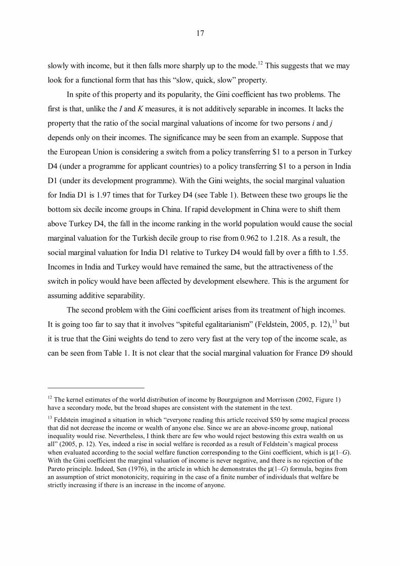
slowly with income, but it then falls more sharply up to the mode.12 This suggests that we may

look for a functional form that has this “slow, quick, slow” property.

In spite of this property and its popularity, the Gini coefficient has two problems. The

first is that, unlike the I and K measures, it is not additively separable in incomes. It lacks the

property that the ratio of the social marginal valuations of income for two persons i and j

depends only on their incomes. The significance may be seen from an example. Suppose that

the European Union is considering a switch from a policy transferring $1 to a person in Turkey

D4 (under a programme for applicant countries) to a policy transferring $1 to a person in India

D1 (under its development programme). With the Gini weights, the social marginal valuation

for India D1 is 1.97 times that for Turkey D4 (see Table 1). Between these two groups lie the

bottom six decile income groups in China. If rapid development in China were to shift them

above Turkey D4, the fall in the income ranking in the world population would cause the social

marginal valuation for the Turkish decile group to rise from 0.962 to 1.218. As a result, the

social marginal valuation for India D1 relative to Turkey D4 would fall by over a fifth to 1.55.

Incomes in India and Turkey would have remained the same, but the attractiveness of the

switch in policy would have been affected by development elsewhere. This is the argument for

assuming additive separability.

The second problem with the Gini coefficient arises from its treatment of high incomes.

It is going too far to say that it involves “spiteful egalitarianism” (Feldstein, 2005, p. 12),13 but

it is true that the Gini weights do tend to zero very fast at the very top of the income scale, as

can be seen from Table 1. It is not clear that the social marginal valuation for France D9 should

12 The kernel estimates of the world distribution of income by Bourguignon and Morrisson (2002, Figure 1) have a secondary mode, but the broad shapes are consistent with the statement in the text. 13 Feldstein imagined a situation in which “everyone reading this article received $50 by some magical process that did not decrease the income or wealth of anyone else. Since we are an above-income group, national inequality would rise. Nevertheless, I think there are few who would reject bestowing this extra wealth on us all” (2005, p. 12). Yes, indeed a rise in social welfare is recorded as a result of Feldstein’s magical process when evaluated according to the social welfare function corresponding to the Gini coefficient, which is µ(1–G). With the Gini coefficient the marginal valuation of income is never negative, and there is no rejection of the Pareto principle. Indeed, Sen (1976), in the article in which he demonstrates the µ(1–G) formula, begins from an assumption of strict monotonicity, requiring in the case of a finite number of individuals that welfare be strictly increasing if there is an increase in the income of anyone.

18

be 2.14 times that for the US D9. We may want to allow for the possibility that the social

marginal valuation remains strictly above a positive value as income tends to infinity.

4. Towards a new approach

The previous discussion provides the rationale that leads us to propose a new measure.

The objective is to design a measure that combines the “slow, quick, slow” empirical property

of the Gini coefficient with additive separability, while allowing for a strictly positive social

marginal valuation of income at all income levels. The second motivation for devising a new

measure goes back to the objective of integrating the analysis of poverty and inequality. This

can be achieved by assigning to a particular income level the role of a poverty line, a feature

not shown by any of the measures considered so far. The identification of a poverty threshold

within the social welfare function helps us to show that concern about poverty may either be

because incomes are unequally distributed and some people fall below the poverty line or

because mean income is below the poverty line (or both). Put differently, poverty may occur

even if everyone has the same income, if a society is globally poor. Clearly this depends on

how the poverty line is defined. A society could not be globally poor if the poverty line were

taken as some percentage (less than 100 per cent) of the mean income. In what follows, we

consider a variety of approaches. That just described, often referred to as a “relative” poverty

line may be contrasted with “absolute” poverty lines that are independent of mean income,

although we should note that “absolute” poverty lines are not necessarily constant over time.

As has been stressed by Sen (1983), a standard fixed in one evaluative space, such as that of

capabilities, may imply a poverty line in terms of income that varies over time.

In order to achieve the objectives of greater flexibility and of integrating poverty and

inequality, we need to introduce a number of parameters governing the form of the social

welfare function. Readers may, quite understandably, resist being asked to consider a measure

of inequality that requires them to think first about the values of different parameters. The

popularity of the Gini coefficient is in part due to the fact that it requires no parameter be

specified. However, this does not mean that there are no implicit value judgements underlying

the Gini coefficient; we have just shown that its properties can be challenged. The virtue of

parameterisation, as argued in Atkinson (1970), is that it forces the user to make explicit

19

choices about the instrument of evaluation and it allows readily for differences of view about

the importance of redistribution.

We propose the following four-parameter measure of global social welfare:

[ ]∑∑

+

βλ−≡=Σ −δβδ−δβ

)()(

1ln

110

i

y

ii iieey

nW

n (1)

where β is positive and has the dimension of 1/income, δo and δ have the dimension of income,

and λ is a non-negative pure number. As a consequence, the expression Σ used to evaluate

total world welfare has the dimension of income.14

The specification of (1) embodies the two key steps described earlier – the shape of the

individual function, and the calculation of the welfare cost – both of which involve

assumptions. The first step is that we have adopted an exponential form that tilts the measure

in direction of K rather than I. Indeed, as shown below, the Kolm measure may be seen in

terms of a limiting case of (1). In this sense, Σ is an absolute measure.15 The first element in (1)

is the mean income, from which the second term capturing the unequal distribution of income,

weighted by the parameter λ, is subtracted. In this sense, too, Σ is an absolute measure. Note

that Σ can be negative.

How can the different parameters be interpreted? It is useful to begin with the first

derivative:

+λ+= δ−β

δ−δβ

)(

)(

11

1'

0

iyie

e

nW (2)

As before, we ignore the divisor n and refer to the square bracket as the individual social

marginal valuation of income for person i. There are four parameters in (1) and (2), but δ0 only

plays an instrumental role; unless explicitly signalled, we assume that δ=δ0 , reducing to three

the parameters that need to be chosen: β, δ and λ.

14 The social welfare function is assumed to be defined over incomes, not individual utilities. We are not asserting that there exists a well-behaved utility function such that the private marginal valuation of income can be written in this form. 15 It would be an interesting extension to consider a version closer to the I measure. We are grateful to Peter Hammond for the suggestion that we seek to derive the K or I indices as a limiting case.

20

The parameter λ captures the differing importance attached to distributional concerns.

If no weight is attached to distribution, then one simply sets 0=λ , the social marginal

valuation is everywhere 1, and that is the end of the story. The implications of different, non-

zero, choices of λ may be seen from considering the fact that (with δ=δ0 ), the social marginal

valuation falls monotonically from )]1/(1[ βδ−+λ+ e when iy is 0 to 1 as iy tends to infinity.

The social marginal valuation of a person with zero income is at most )1( λ+ times that for the

richest person, so that 4=λ corresponds to a maximum ratio of five, which implies a

maximum socially acceptable loss of 80 per cent from a transfer from the richest to the

poorest. We take this value of λ in the illustrations below, although, in the light of the large

world income differences, this may be regarded as a conservative choice.

The two remaining parameters β and δ determine the nature of our concern for inequality

and poverty. The specification (1) gives a special status to the income level δ and one

interpretation, taken up immediately below, is that of a poverty line. Other interpretations can

however be given, and we show how variations in δ allow the measure to adopt either a Kolm-

like form or a Gini-like form. The parameter β determines the “angularity” of the measure,

which has a natural interpretation in each of the cases, which we now discuss in turn. As in the

following we focus not on incomes but on their ratios to the median m, the actual values of the

parameters in the income space are δm, δ0m and β/m.

The poverty gap

For some people, our concern should be with poverty but not inequality. This position is

exemplified by Feldstein: “I have no doubt about the appropriateness of transferring income to

the very poor … the emphasis should be on eliminating poverty and not on the overall

distribution of income or the general extent of inequality” (2005, p. 12). This position has been

called “charitable conservatism” (Atkinson, 1990). One of the attractions of the measure

proposed here is that it encapsulates the poverty gap if we set δ as the poverty line, with

21

δ=δ0 , and let β tend to infinity. Under these assumptions, the social welfare function (1) is

becomes:16

∑∑ −δλ−=Σ δ=δ∞→β i ii i yn

yn

)](,0max[11

0, (1a)

Thus, world welfare is evaluated as the mean minus λ times the aggregate poverty gap per

head of the total population.17 As may be seen from (2), as β tends to infinity, with δ=δ0 , the

social marginal valuation equals )1( λ+ where income is below δ and 1 where it is above δ.

Distributional concern is concentrated below the poverty line, to an extent that depends on λ.

Where 4=λ , we are subtracting four times the poverty gap from national income: the

multiplication by λ is a way of allowing for the concerns of those who feel that the small size of

the poverty gap, expressed per head of the total population, understates its significance.

A less angular version

With the poverty gap, the social marginal valuation is constant as a function of income

when income is below the poverty line, falls like a stone at δ=y , and is then again constant

for all incomes above the poverty line. For some people, this is too abrupt. We may well want

to taper the marginal valuation as we approach the poverty line, and to recognise that the

needs of the “near-poor”, just above the poverty line, are greater than those of people

comfortably above. The 1991 modification to the Human Development Index (HDI) was based

on the argument that “the idea of diminishing returns to income is now better captured by

giving a progressively lower weight to income beyond the poverty cut-off point, rather than the

16 As β goes to infinity, if yi≥δ the term (1/β)ln[1+exp(β(δ–yi))] in (1) tends to zero; if yi<δ, application of L’Hôpital’s Rule allows the limit to be calculated as (δ–yi). 17 Our formulation of the social welfare function in per capita terms implies that world welfare goes up, ceteris

paribus, whenever the aggregate poverty gap grows less than the population. However, one could argue that what matters in the assessment of poverty is the amount of resources necessary to eliminate poverty, i.e. the absolute aggregate poverty gap, not its value per head. This corresponds to viewing world poverty as measured by the absolute number of the poor rather than their number relative to the total population. Which one of these two conceptions of poverty is chosen has important consequences for the interpretation of the evolution of poverty and welfare, as the absolute and per head aggregate poverty gaps need not move in the same direction. Chakravarty, Kanbur and Mukherjee (2006) attempt to put these two conceptions of poverty together by developing a family of poverty measures which avoid the population replication axiom.

22

zero weight previously given” (United Nations Development Programme, 1991, p. 15).18 The

HDI modification took the form of a fractional weight above the poverty line, but such a “less

angular” version can also be achieved using (1) by retaining δ (= δ0) as the poverty line, and

taking a finite value of β. With β finite, the social marginal valuation changes more smoothly

around δ. This may be seen from the second derivative

++βλ−= δ−βδ−β−

δ−δβ

]1][1[

1'' )()(

)( 0

ii yyiee

e

nW (3)

which has its minimum value (i.e. the steepest downward slope for the marginal valuation) at

δ=iy . Both before and after δ=iy the slope is less. The value of β determines how sharply

the social marginal valuation changes around the point of inflexion. This is illustrated in Figure

5, where we have taken the poverty line as 0.5. The marginal valuation at the poverty line is

)2/1( λ+ , independent of β. All the curves relating to the new measure in Figure 5 pass

through this point since we have taken a common value of 4=λ . (In order to facilitate

comparison, the curves for the Kolm and the constant elasticity measures have been rescaled to

go through this point as well.) The charitable conservative evaluation function is shown by the

broken lines. With 12=β , the function is a “smoothed” version of the poverty gap, giving

some additional weight to people above the poverty line, but the weight falls rapidly away: at

the world median, the social marginal valuation is indistinguishable from that with the poverty

gap. With 4=β , on the other hand, less significance is attached to the poverty line. Those with

incomes up to three times the poverty line receive a perceptible additional weight, which is

similar to that assigned to them by the (rescaled) constant elasticity index I with 1=ε ; for

higher incomes, the social marginal valuation stabilises at 1, the lower bound for the new

measure, while it keeps declining for the index I. With 4=β , those below the poverty line get

lower weight, relative not only to the poverty gap version and the function with higher values

of β but also to the constant elasticity measure.

18 We owe this quotation to Anand and Sen (2000), who present an extensive (and sympathetic) critique of the treatment of the social marginal valuation of income in successive versions of the HDI.

23

Towards an inequality measure

If we cease to regard δ as the poverty line, the new measure can represent the views of

those who are concerned with overall inequality. If we set 0=δ (and 00 =δ ), then there is no

interior point of inflexion, and (with 4=λ ) the social marginal valuation of income has the

form shown in Figure 6 by the three curves starting from the same value 3 (the social valuation

at zero income is )2/1( λ+ ). The three curves are based on different values of β and illustrate

different speeds of approach to the limiting value of 1: the greater β, the more rapidly the

weight attributed to higher incomes converges to 1. For the range of incomes shown in Figure

6, the curve with the lowest value of β (0.5) has some similarity with the Kolm index with an

elasticity of 1/5 at the median (after rescaling so that it also starts from 3 when income is nil).

There is indeed a close relation with the Kolm index. If we hold 00 =δ , but allow δ to

tend to minus infinity, the individual social marginal valuation of income becomes )1( iye

β−λ+ ,

which for large λ approaches the Kolm form with β corresponding to κ in equation (K). As δ

tends to minus infinity, equation (1) becomes:

∑∑ β−=δ−∞→δ β

λ−=Σi

y

i iie

ny

n

110, 0

(1b)

The separation of δ0 and δ is introduced to allow this limit to be taken. (The limit may be seen

from (1) by regarding )exp(βδ as the denominator, and applying L’Hôpital’s Rule.) Arrival at

a form similar to the Kolm index underlines the absolute rather than relative nature of our

generalisation, but we should stress the difference remaining where λ is finite: as income goes

to infinity, the social marginal valuation of income goes to zero in the case of the Kolm index

while it approaches one with (1b). Thus, the social evaluation of an extra dollar accruing to the

poorest person relative to an extra dollar accruing to the richest person approaches infinity

with the Kolm index, while it is at most )1( λ+ with our formulation.

The similarity with the Kolm index is illustrated by the curves in the upper part of Figure

6. According to Σ, the elasticity with respect to income of the social marginal valuation of

income, defined positively, is:

]1][1[

)()()()(

)(

0

0

δ−δβδ−βδ−β−

δ−δβ

λ+++λβ=η

eee

yey

ii yy

ii (4)

24

The two curves in Figure 6 marked by crosses and squares virtually coincide, within the shown

income range, with the continuous curves which correspond to the Kolm indices having the

same elasticity at the median as given by (4), rescaled so to start from the same value at zero

income. (The two curves would however depart from their Kolm counterparts at some higher

level of income.)

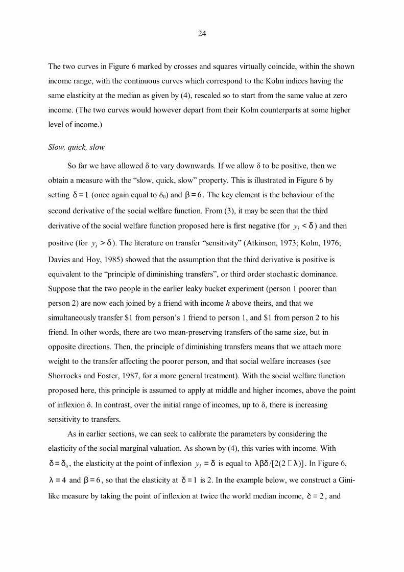
Slow, quick, slow

So far we have allowed δ to vary downwards. If we allow δ to be positive, then we

obtain a measure with the “slow, quick, slow” property. This is illustrated in Figure 6 by

setting 1=δ (once again equal to δ0) and 6=β . The key element is the behaviour of the

second derivative of the social welfare function. From (3), it may be seen that the third

derivative of the social welfare function proposed here is first negative (for δ<iy ) and then

positive (for δ>iy ). The literature on transfer “sensitivity” (Atkinson, 1973; Kolm, 1976;

Davies and Hoy, 1985) showed that the assumption that the third derivative is positive is

equivalent to the “principle of diminishing transfers”, or third order stochastic dominance.

Suppose that the two people in the earlier leaky bucket experiment (person 1 poorer than

person 2) are now each joined by a friend with income h above theirs, and that we

simultaneously transfer $1 from person’s 1 friend to person 1, and $1 from person 2 to his

friend. In other words, there are two mean-preserving transfers of the same size, but in

opposite directions. Then, the principle of diminishing transfers means that we attach more

weight to the transfer affecting the poorer person, and that social welfare increases (see

Shorrocks and Foster, 1987, for a more general treatment). With the social welfare function

proposed here, this principle is assumed to apply at middle and higher incomes, above the point

of inflexion δ. In contrast, over the initial range of incomes, up to δ, there is increasing

sensitivity to transfers.

As in earlier sections, we can seek to calibrate the parameters by considering the

elasticity of the social marginal valuation. As shown by (4), this varies with income. With

0δ=δ , the elasticity at the point of inflexion δ=iy is equal to )]2(2/[ λ+λβδ . In Figure 6,

4=λ and 6=β , so that the elasticity at 1=δ is 2. In the example below, we construct a Gini-

like measure by taking the point of inflexion at twice the world median income, 2=δ , and

25

setting 3=β ; this leaves the elasticity at the point of inflexion unchanged at 2, but gives a

much lower elasticity of 0.11 at the median income. With higher values of δ, the flatter, initial

section applies over a wider range. Indeed, by letting δ go to infinity, we obtain as a limiting

case that of distributional indifference.

On the interpretation of the new measure

The new measure proposed here has been motivated as embodying a desired pattern of

change in the social marginal valuation of income. But how is the new measure to be

interpreted? Its interpretation may be aided by re-arranging the expression for social welfare.

By adding and subtracting from (1) the term [ ])()( 1ln0 µ−δβδ−δβ +βλ

ee , we can treat social welfare

as being made up of two components:

++

βλ−µΣ=σ−µΣ=Σ ∑ µ−δβ

−δβδ−δβ

)(

)()(

1

1ln

1)()( 0

i

y

e

e

ne

i

(5)

The first term on the right hand side of (5), )(µΣ is the level of social welfare attained if

everyone has an income equal to the mean µ. In general, this level of social welfare is less than

µ, although it approaches µ as the mean tends to infinity (with the poverty gap, it is equal to µ

once the mean passes the poverty line). This reflects the fact that it is a welfare measure, and

that there are diminishing returns in the transformation of income into welfare. The second

term, denoted by σ, represents the costs of income differences: it may be seen that the term

reduces to zero where all incomes are equal to the mean.

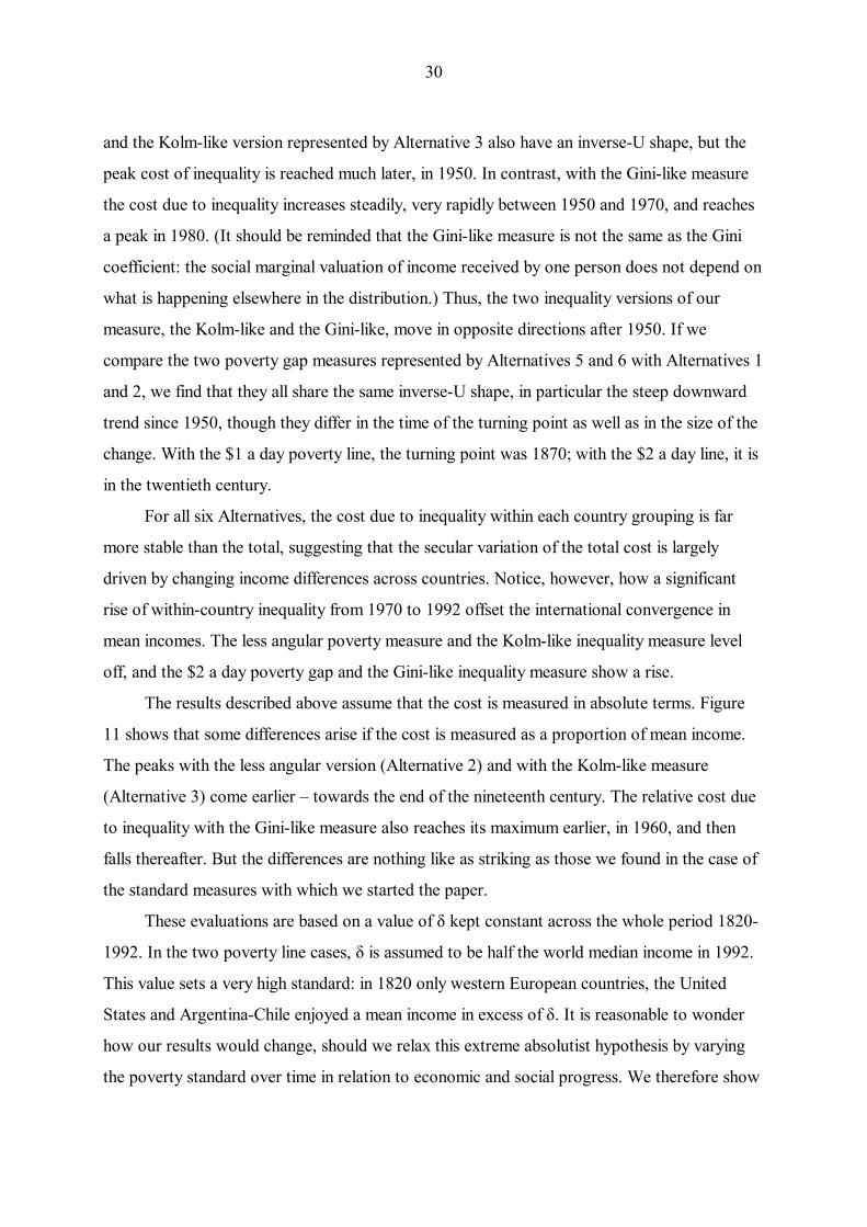
The way in which our new measure differs from earlier approaches can be illustrated by

taking the simple example in Figure 7. If there are two people, with incomes (measured on the

horizontal axis) as shown, and mean µ, the achieved level of social welfare is given by the point

C (the midpoint). Welfare is measured on the vertical axis. The I and K measures proceed by

calculating the equally-distributed equivalent income ye (obtained by reading across

horizontally from C to the point D), and the cost of inequality is the loss CD. Unlike the I and

K social welfare functions, however, the new measure developed here has the same dimension

as income. This implies that we can directly compare the level of welfare Σ with the mean

income µ, and there is no need to introduce the equally-distributed equivalent income. The

26

overall difference between µ and Σ, GC, is made up of two components, GF and FC: GF

reflects the diminishing returns in the transformation of income into welfare, and shrinks as

income grows; FC measures the cost of inequality, which is the second term in (5).

In the case of the poverty gap, the curve in Figure 7 becomes a kinked line, coinciding

with the 45o line from the level δ of the poverty income onwards. In this case, the distance GC

is λ times the aggregate poverty gap per head. This gap consists, potentially, of two

components, either of which may be zero. Where the mean income is above the poverty line,

poverty is due entirely to the unequal distribution of income. If the mean income is below the

poverty line, there can be both aggregate (corresponding to the difference between µ and

)(µΣ ) and distributional poverty. There can remain aggregate poverty even where incomes are

equalised. Indeed, if everyone has an income below the poverty line, then the component FC

disappears even though income differences remain (since the poverty gap is unaffected by

transfers of income among people below the poverty line). The problem of poverty can

therefore be seen as a problem of distribution and/or a problem of the overall level of income.

These observations highlight the crucial role played by δ, when seen as the poverty line. δ (and

δ0) could be defined as a fraction of mean income – a purely relative approach – that we do not

explore here. On an absolute approach, δ (and δ0) is independent of mean income, but, as

noted earlier, this does not imply that it should be kept constant over a long period of time.

Where the underlying concern relates to a more fundamental space, such as the achievement of

a level of functionings, the necessary level of income may be changing as a result of economic

and social progress. We return to this issue in the next section.

In the general case, we are not concerned with the component GF, but only with the

costs of inequality FC. With regard to the latter it is instructive to see how our measure departs

from Kolm’s absolute approach. The Kolm index K measures the costs of inequality as the

absolute difference between the mean and the equally-distributed equivalent income:

KeyK −µ= . With expression (5), we express the cost of inequality as the difference between

the social welfare at the mean )(µΣ and the social welfare for the actual income distribution Σ.

As by definition the social welfare at the equally-distributed equivalent income equals Σ, we are

basically taking )()( eyΣ−µΣ instead of ey−µ as the cost of the unequal distribution of

27

income. For our Kolm-like measure defined by (1b), this term equals βλ−ββµ− /)1( Kee ,

where K is the Kolm index with β=κ . For given mean income the two measures generate the

same ranking, but the cost of inequality defined here is smoothed out by a rise in mean income.

Raising all incomes by $1 leaves the Kolm index unchanged by construction but reduces the

costs of inequality with our Kolm-like measure, and it does so at a decreasing rate as mean

income rises: the richer the economy, the less an extra $1 is worth.

Lastly, it is worth noting that our inequality measure σ is decomposable by population

subgroups (see Cowell, 1980; Shorrocks, 1980):

∑∑

++

βλ+σ=σ µ−δβ

µ−δβδ−δβ

j jj jje

ewew

k

)(

)()(

1

1ln0 (6)

where subscript j refers to the J mutually exclusive subgroups of the population, and wj is the

population share of subgroup j. The first term on the right hand side of (6) is the population

weighted average of within-group inequalities, while the second term is the between-group

inequality, that is the inequality calculated after assuming that to each member in a group is

attributed the group mean income. In the case of the poverty gap measure (1a), the

decomposition is:

∑∑ µ−δλ−µ−δλ+σ=σ δ=δ→∞β j jjj jj ww )](,0max[)](,0max[0,

(6a)

When the overall mean is above the poverty line, the between-group component is λ times the

weighted average of the aggregate poverty indicator, that is the difference )( jµ−δ if positive;

when the overall mean falls short of the poverty line, the aggregate poverty indicator must be

subtracted from this sum. The decomposability property proves useful in the analysis of world

income distribution to evaluate the contribution of a country, or a group of countries, to the

evolution of global inequality.

Summary

Our aim in introducing the new measure has been to provide a more flexible approach to

measuring inequality and poverty. This allows us to “blend” different concerns, rather than

treat them as incommensurable. The price has been the introduction of four parameters – three,

if we consider only those playing a substantive role – each of which has to be specified, but

which allow us to encompass a variety of different positions regarding the first of the two key

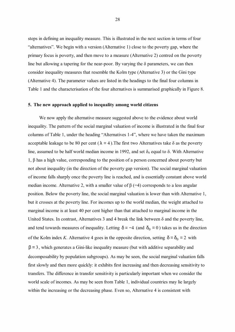
28

steps in defining an inequality measure. This is illustrated in the next section in terms of four

“alternatives”. We begin with a version (Alternative 1) close to the poverty gap, where the

primary focus is poverty, and then move to a measure (Alternative 2) centred on the poverty

line but allowing a tapering for the near-poor. By varying the δ parameters, we can then

consider inequality measures that resemble the Kolm type (Alternative 3) or the Gini type

(Alternative 4). The parameter values are listed in the headings to the final four columns in

Table 1 and the characterisation of the four alternatives is summarised graphically in Figure 8.

5. The new approach applied to inequality among world citizens

We now apply the alternative measure suggested above to the evidence about world

inequality. The pattern of the social marginal valuation of income is illustrated in the final four

columns of Table 1, under the heading “Alternatives 1-4”, where we have taken the maximum

acceptable leakage to be 80 per cent ( 4=λ ).The first two Alternatives take δ as the poverty

line, assumed to be half world median income in 1992, and set δ0 equal to δ. With Alternative

1, β has a high value, corresponding to the position of a person concerned about poverty but

not about inequality (in the direction of the poverty gap version). The social marginal valuation

of income falls sharply once the poverty line is reached, and is essentially constant above world

median income. Alternative 2, with a smaller value of β (=4) corresponds to a less angular

position. Below the poverty line, the social marginal valuation is lower than with Alternative 1,

but it crosses at the poverty line. For incomes up to the world median, the weight attached to

marginal income is at least 40 per cent higher than that attached to marginal income in the

United States. In contrast, Alternatives 3 and 4 break the link between δ and the poverty line,

and tend towards measures of inequality. Letting 4−=δ (and 00 =δ ) takes us in the direction

of the Kolm index K. Alternative 4 goes in the opposite direction, setting 20 =δ=δ with

3=β , which generates a Gini-like inequality measure (but with additive separability and

decomposability by population subgroups). As may be seen, the social marginal valuation falls

first slowly and then more quickly: it exhibits first increasing and then decreasing sensitivity to

transfers. The difference in transfer sensitivity is particularly important when we consider the

world scale of incomes. As may be seen from Table 1, individual countries may lie largely

within the increasing or the decreasing phase. Even so, Alternative 4 is consistent with

29

substantial redistribution within the United States: the social marginal valuation for D1 is more

than three times that for the US median.

These four Alternative measures are applied to the world income estimates of the BM

database. Figure 9 shows the evolution of world social welfare from 1820 to 1992, where, as

in equation (1), welfare has the dimension of per capita income, and we express its value as a

percentage of the world median income in 1992. As noted earlier, welfare may be negative, and

this was the case for all four alternatives until the beginning of the twentieth century. In the

case of the poverty line measures, we are applying a contemporary (1992) standard, so that it

is scarcely surprising that the earlier values are so low, but the inequality measures are also

absolute in the sense that we described in the previous section. This applies not only to

Alternative 3, approaching the Kolm index, but also to the Gini-like Alternative 4. Indeed the

Gini-like measure is initially off the scale. All four measures indicate a considerable

improvement over the period, driven by the growth of mean income (the thick top line).

However, while the upward tendency was similar, the rates of increase in social welfare

differed from those in mean income. For example, the (absolute) annual increase in mean

income between 1980 and 1992 was double that between 1890 and 1910, but the rise in social

welfare using the Gini-like index was only a quarter higher. Distributionally-adjusted income,

as with our social welfare measure, may give a rather different picture of different historical

periods.

The absolute cost of inequality σ is given in Figure 10, again expressed as a percentage

of the 1992 world median, so that a value of 100 corresponds to a cost of US $1,712 per

person. There are six panels in Figure 10: one for each of the four Alternatives considered, and

one each for the poverty gap measures defined in (1a) with δ set at 0.5 and 1 (referred to as

Alternatives 5 and 6). Notice that these latter two values correspond to the $1 a day and $2 a

day poverty lines, respectively, as defined by Bourguignon and Morrisson (2002). In all six

panels of Figure 10 the continuous lines correspond to the total cost of inequality, while the

dashed lines indicate the within-country inequality, that is the population-weighted average of

inequality calculated within the 33 countries or groups of countries included in the BM

database. With Alternative 1, whose parameters lead in the direction of the poverty gap, we

see that the cost due to inequality rises until 1890, and then declines, more rapidly after the

Second World War. The time path with the less angular version represented by Alternative 2

30

and the Kolm-like version represented by Alternative 3 also have an inverse-U shape, but the

peak cost of inequality is reached much later, in 1950. In contrast, with the Gini-like measure

the cost due to inequality increases steadily, very rapidly between 1950 and 1970, and reaches

a peak in 1980. (It should be reminded that the Gini-like measure is not the same as the Gini

coefficient: the social marginal valuation of income received by one person does not depend on

what is happening elsewhere in the distribution.) Thus, the two inequality versions of our

measure, the Kolm-like and the Gini-like, move in opposite directions after 1950. If we

compare the two poverty gap measures represented by Alternatives 5 and 6 with Alternatives 1

and 2, we find that they all share the same inverse-U shape, in particular the steep downward

trend since 1950, though they differ in the time of the turning point as well as in the size of the

change. With the $1 a day poverty line, the turning point was 1870; with the $2 a day line, it is

in the twentieth century.

For all six Alternatives, the cost due to inequality within each country grouping is far

more stable than the total, suggesting that the secular variation of the total cost is largely

driven by changing income differences across countries. Notice, however, how a significant

rise of within-country inequality from 1970 to 1992 offset the international convergence in

mean incomes. The less angular poverty measure and the Kolm-like inequality measure level

off, and the $2 a day poverty gap and the Gini-like inequality measure show a rise.

The results described above assume that the cost is measured in absolute terms. Figure

11 shows that some differences arise if the cost is measured as a proportion of mean income.

The peaks with the less angular version (Alternative 2) and with the Kolm-like measure

(Alternative 3) come earlier – towards the end of the nineteenth century. The relative cost due

to inequality with the Gini-like measure also reaches its maximum earlier, in 1960, and then

falls thereafter. But the differences are nothing like as striking as those we found in the case of

the standard measures with which we started the paper.

These evaluations are based on a value of δ kept constant across the whole period 1820-

1992. In the two poverty line cases, δ is assumed to be half the world median income in 1992.

This value sets a very high standard: in 1820 only western European countries, the United

States and Argentina-Chile enjoyed a mean income in excess of δ. It is reasonable to wonder

how our results would change, should we relax this extreme absolutist hypothesis by varying

the poverty standard over time in relation to economic and social progress. We therefore show

31

in Figure 12 the consequences of recomputing our measure retaining the value of δ for 1992,

but assuming that it grew over time as the median world income. This amounts to applying the

values indicated in Table 1 to the median income in each year, rather than to the median

income in 1992, but it should be stressed that we are not assuming that the poverty line is

proportionate to median, or mean, incomes; rather we are taking the increase in median income

as a reference point. The (externally-derived) time-variation in δ may involve a faster or slower

rate of growth. All other parameters are kept unchanged. As shown in Figure 12, under a time-

varying δ the secular pattern of world income inequality looks considerably different from the

one reported earlier for all poverty-type measures, both Alternatives 1 and 2, and Alternatives

5 and 6: the inverse-U shape turns into a steadily ascending trend, which only flattens out after

1980. The impact is instead barely visible on the two inequality-type measures, except for the

upward trend of the Gini-like measure, now continuing even after 1970. Assuming a time-

varying δ affects also the within-country component, which tends to account for a much larger

share of the overall inequality: in Alternatives 1 and 5 it almost wipes out the between-country

component.

To sum up, contrary to what is suggested by the earlier analysis using the standard

inequality indices, the conclusions do depend very much on distributional judgments.

6. Conclusions

The effects of “globalisation” on world income inequality have been much debated in

recent years. In the literature, as noted by Anand and Segal, “no consensus emerges concerning

the direction of change in global inequality in the last twenty to thirty years” (2008, p. 61).

Some commentators have stressed the impressive growth performance of some emerging

economies, like China, India and other countries in South East Asia, and have concluded that

world inequality and poverty must have decreased. Others have countered that these

impressive rates of growth have not yet translated into absolute increases of size comparable to

that of developed economies, given the very different levels of GDP per head. Thus, world

income gaps must have risen. In this paper, we have argued that – before we can make such

judgments – we need to re-examine the foundations of inequality measurement. The sheer scale

of global income differences means, in our view, that we cannot simply carry over the tools

32

applied to inequality measurement at a domestic level. In the discourse about global justice, we

have to consider both poverty and inequality and their inter-relation, and we have to consider

the different meanings of “absolute” and “relative”.

Differences of view about the evolution of world inequality and poverty stem in part

from differences as to how they should be measured. Adopting for the purposes of this paper a

welfarist approach (without endorsing this as the only possible approach), we have sought to

provide a framework for considering the cost of world inequality and poverty that

encompasses different types of concern.19 In part, these differences of view are presentational:

whether the cost is expressed in absolute terms or relative to mean incomes. This may make a

rhetorical difference, but otherwise seems inessential. Our first findings, in Section 2,

suggested that the differences in conclusions regarding changes in world inequality could be

largely attributed to how the cost is expressed. However, we argued in Section 3 that the

existing measures of inequality impose too tight constraints on the way in which the social

marginal valuation varies with income; moreover they provide no ready means to integrate the

analysis of poverty and inequality.

In order to encompass the extent of global income differences and to allow for concerns

about poverty as well as inequality, we proposed in Section 4 a new parameterised measure of

global social welfare. This measure has, in a sense explained, an absolute structure (and it

would be interesting to consider the parallel, relative measure), but it is sufficiently flexible to

include a variety of different value systems and to incorporate a poverty line. By including

several approaches within a single measure, we can not only understand better their inter-

relation but also obtain measures that “blend” different concerns. People differ, for example, in

the relative importance they attach to poverty and inequality. This difference appears

fundamental, but can be embedded within the new measure proposed here. Letting one of the

key parameters increase allows the measure to take on a poverty gap form, whereas lower

values permit a less angular version of the poverty gap, tapering the measure for the near-poor.

19 The new measure has applications outside the present field. In a paper presented at the Conference in honour of Claude Henry in Paris in December 2006, one of us (ABA) discussed the implications of the functional form for the choice of social discount rate in measuring the costs of global warming. Adoption of a non-constant elasticity form seems an evident way of resolving some of the disagreements in this area.

33

If we allow other parameters to vary, we can introduce more general concerns about

inequality. These may follow the pattern of standard welfare-based measures, with declining

sensitivity to transfers as we move up the income scale. Or, they may exhibit first increasing

and then decreasing sensitivity to transfers, mimicking the Gini coefficient but with the

property of additive separability (and subgroup decomposability). The new measure can

accommodate a constant poverty line or one varying over time in relation to economic and

social development, an alternative that has considerable consequences for the interpretation of

the evolution of the world income distribution. Finally, we can vary the overall weight attached

to distributional issues. A person may, for example, be concerned about poverty but not attach

a great deal of weight to this consideration, relative to the size of the cake. Or a person may

feel that, in the context of world poverty, little weight should be attached to additional income

attached to those at the very top of the distribution. Stated more pragmatically, the new

measure can exhibit a willingness to redistribute within rich countries without magnifying to an

implausible degree the willingness to make transfers across the whole spectrum of world

incomes.

34

Table 1 World incomes in 1992 expressed relative to the world median and social marginal valuation of income

Social marginal valuation of income Income relative to world median

Decile groups

Constant elasticity ε = 2

Constant elasticity ε = 1

Constant elasticity ε = 1/8

Kolm index

elasticity κm = 1/8 at world median

Gini coeffi-cient (1)

Alterna-tive 1

Direction of pov-erty gap

λ=4 β=12

δ=δ0=0.5

Alterna-tive 2

Less angular

λ=4 β=4 δ=δ0=0.5

Alterna-tive 3

Direction of Kolm λ=4 β=2

δ=-4 δ0=0

Alterna-tive 4

Gini-like λ=4 β=3 δ=δ0=2

0.15 46 African countries D1 44.444 6.667 1.268 1.112 1.988 4.893 2.850 2.571 1.036 0.20 Nigeria D2 25.000 5.000 1.223 1.105 1.968 4.846 2.759 2.388 1.036 0.28 India D1 12.755 3.571 1.172 1.094 1.892 4.687 2.592 2.131 1.035 0.34 Philippines-Thailand D1 8.651 2.941 1.144 1.086 1.760 4.445 2.451 1.963 1.034 0.40 Indonesia D1 6.250 2.500 1.121 1.078 1.711 4.034 2.299 1.815 1.033 0.48 Mexico D1 4.340 2.083 1.096 1.067 1.578 3.207 2.086 1.642 1.031 0.59 Philippines-Thailand D3 2.873 1.695 1.068 1.053 1.371 1.994 1.790 1.446 1.028 0.68 Russia D1 2.163 1.471 1.049 1.041 1.294 1.400 1.564 1.315 1.024 0.76 China D5 1.731 1.316 1.035 1.030 1.211 1.158 1.384 1.216 1.020 0.80 Indonesia D3 1.563 1.250 1.028 1.025 1.162 1.096 1.304 1.173 1.017 0.88 Egypt D4 1.291 1.136 1.016 1.015 1.059 1.031 1.163 1.095 1.012 1.01 North Africa D4 0.980 0.990 0.999 0.999 0.995 0.999 0.989 0.993 0.999 1.11 Turkey D4 0.812 0.901 0.987 0.986 0.962 0.993 0.894 0.931 0.986 1.27 37 Latin American countries D7 0.620 0.787 0.971 0.967 0.866 0.991 0.796 0.853 0.956 1.40 45 Asian countries D6 0.510 0.714 0.959 0.951 0.807 0.990 0.749 0.807 0.921 1.49 Mexico D5 0.450 0.671 0.951 0.941 0.759 0.990 0.728 0.781 0.891 1.57 Portugal-Spain D1 0.406 0.637 0.945 0.931 0.737 0.990 0.714 0.761 0.860 1.68 Poland D4 0.354 0.595 0.937 0.919 0.709 0.990 0.701 0.739 0.809 1.76 US D1 0.323 0.568 0.932 0.909 0.681 0.990 0.695 0.726 0.767 2.00 Brazil D7 0.250 0.500 0.917 0.882 0.602 0.990 0.684 0.696 0.624 2.36 Germany D1 0.180 0.424 0.898 0.844 0.516 0.990 0.679 0.672 0.419 2.77 US D2 0.130 0.361 0.880 0.802 0.472 0.990 0.677 0.659 0.283 3.03 Italy D2 0.109 0.330 0.871 0.776 0.425 0.990 0.677 0.655 0.244 3.44 Germany D2 0.085 0.291 0.857 0.737 0.402 0.990 0.677 0.651 0.219 7.02 Italy D5 0.020 0.142 0.784 0.471 0.238 0.990 0.677 0.649 0.208 9.19 US D5 0.012 0.109 0.758 0.359 0.164 0.990 0.677 0.649 0.208 10.01 Germany D7 0.010 0.100 0.750 0.324 0.149 0.990 0.677 0.649 0.208 11.08 US D6 0.008 0.090 0.740 0.284 0.131 0.990 0.677 0.649 0.208 14.79 France D9 0.005 0.068 0.714 0.178 0.069 0.990 0.677 0.649 0.208 20.66 US D9 0.002 0.048 0.685 0.086 0.032 0.990 0.677 0.649 0.208 38.79 US D10 0.001 0.026 0.633 0.009 0.005 0.990 0.677 0.649 0.208

Source: authors’ elaboration on the BM database.. (1) As income refers to the mean income of each decile group (as a ratio to the world median), in the expression for the social marginal valuation of income the term (2i–1)/n represents the mean rank of all people in the decile group and is calculated as the sum of the cumulative share of all groups poorer than the one indicated and half the population share of the group itself.

35

Figure 1 Evolution of world inequality and poverty, 1820-1992: Standard measures

0

25

50

75

100

1820 1840 1860 1880 1900 1920 1940 1960 1980 2000

Per cent

0

50

100

150

200

Percentage ratio to 1992 world median

Poverty headcountGini coefficientAbsolute Gini coefficient (RH axis)

Source: authors’ elaboration on the BM database..

Figure 2 Evolution of world inequality, 1820-1992: Different parameter values

0

20

40

60

80

1820 1840 1860 1880 1900 1920 1940 1960 1980 2000

Per cent

0

20

40

60

80Gini coefficientI with ε = 2I with ε = 1I with ε = 1/8

Source: authors’ elaboration on the BM database..

36

Figure 3 Evolution of world inequality, 1820-1992: Absolute measures

0

50

100

150

200

250

1820 1840 1860 1880 1900 1920 1940 1960 1980 2000

Percentage ratio to 1992 world median

0

50

100

150

200

250µI with ε = 2µI with ε = 1µI with ε = 1/8Absolute Gini coefficientK with elasticity = 2K with elasticity = 1K with elasticity = 1/8

Source: authors’ elaboration on the BM database.. The elasticity of the index K is computed at the 1992 world

median.

Figure 4 Social marginal valuation of income

0.0

0.5

1.0

1.5

2.0

2.5

0.0 0.5 1.0 1.5 2.0 2.5Income relative to world median

I [ε =1]

K [κm =1/8]

I [ε =1/8]

Implicit in world Gini

Source: authors’ elaboration on the BM database.. All values of the social marginal valuation of income are

normalised by the value it takes at the world median.

37

Figure 5 Social marginal valuation of income with new measure: poverty line version

0.0

1.0

2.0

3.0

4.0

5.0

6.0

0.0 0.5 1.0 1.5 2.0 2.5Income relative to world median

I [ε =1]

K [κm =1/8] Σ [λ=4, β=4, δ=δ0=0.5]

Charitable conservative Σ [λ=4, β=∞, δ=δ0=0.5]

Σ [λ=4, β=12, δ=δ0=0.5]

Figure 6 Social marginal valuation of income with new measure: inequality version

0.0

1.0

2.0

3.0

4.0

5.0

6.0

0.0 0.5 1.0 1.5 2.0 2.5Income relative to world median

Σ [λ=4, β=12, δ=δ0=0]K [κm =0.2]

Σ [λ=4, β=0.5, δ=−2, δ0=0], η=0.272

Σ [λ=4, β=0.5, δ=−10,δ0=0], η=0.352

Σ [λ=4, β=0.5, δ=δ0=0]

Σ [λ=4, β=4, δ=δ0=0]

Σ [λ=4, β=6, δ=δ0=1]

K [κm =0.352]

K [κm =0.272]

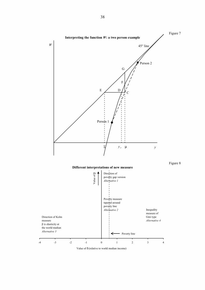
38

Figure 7 Interpreting the function W: a two person example

CDE

45° line

Σ y e

Person 2

Person 1

y

W

µ

G

F

Figure 8 Different interpretations of new measure

-4 -3 -2 -1 0 1 2 3 4

Value of δ (relative to world median income)

Value of β Direction of

poverty gap versionAlternative 1

Poverty line

Direction of Kolm measureβ is elasticity at the world medianAlternative 3

Inequality measure of Gini typeAlternative 4

Poverty measure tapered around poverty lineAlternative 2

39

Figure 9 Evolution of world social welfare, 1820-1992: Alternatives 1-4

-600

-300

0

300

1820 1840 1860 1880 1900 1920 1940 1960 1980 2000

Percentage ratio to 1992 world median .

-600

-300

0

300

Alternative 1: Direction of poverty gap Alternative 2: Less angularAlternative 3: Direction of Kolm Alternative 4: Gini-likeMean

Source: authors’ elaboration on the BM database..

40

Figure 10 Evolution of the absolute cost of world inequality, 1820-1992: Alternatives 1-4

Alternative 1: Direction of poverty gap

0

25

50

75

100

1820 1840 1860 1880 1900 1920 1940 1960 1980 2000

Percentage ratio to 1992 world median

Alternative 2: Less angular

0

25

50

75

100

1820 1840 1860 1880 1900 1920 1940 1960 1980 2000

Percentage ratio to 1992 world median

Alternative 3: Direction of Kolm

0

25

50

75

100

1820 1840 1860 1880 1900 1920 1940 1960 1980 2000

Percentage ratio to 1992 world median

Alternative 4: Gini-like

0

100

200

300

400

1820 1840 1860 1880 1900 1920 1940 1960 1980 2000

Percentage ratio to 1992 world median

Alternative 5: Poverty gap 1$ a day

0

25

50

75

100

1820 1840 1860 1880 1900 1920 1940 1960 1980 2000

Percentage ratio to 1992 world median

Alternative 6: Poverty gap 2$ a day

0

50

100

150

200

1820 1840 1860 1880 1900 1920 1940 1960 1980 2000

Percentage ratio to 1992 world median

Total Within-country

Source: authors’ elaboration on the BM database..

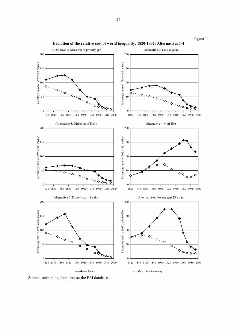
41

Figure 11 Evolution of the relative cost of world inequality, 1820-1992: Alternatives 1-4

Alternative 1: Direction of poverty gap

0

50

100

150

200

1820 1840 1860 1880 1900 1920 1940 1960 1980 2000

Percentage ratio to 1992 world median

Alternative 2: Less angular

0

50

100

150

200

1820 1840 1860 1880 1900 1920 1940 1960 1980 2000

Percentage ratio to 1992 world median

Alternative 3: Direction of Kolm

0

50

100

150

200

1820 1840 1860 1880 1900 1920 1940 1960 1980 2000

Percentage ratio to 1992 world median

Alternative 4: Gini-like

0

50

100

150

200

1820 1840 1860 1880 1900 1920 1940 1960 1980 2000

Percentage ratio to 1992 world median

Alternative 5: Poverty gap 1$ a day

0

50

100

150

200

1820 1840 1860 1880 1900 1920 1940 1960 1980 2000

Percentage ratio to 1992 world median

Alternative 6: Poverty gap 2$ a day

0

50

100

150

200

1820 1840 1860 1880 1900 1920 1940 1960 1980 2000

Percentage ratio to 1992 world median

Total Within-country

Source: authors’ elaboration on the BM database..

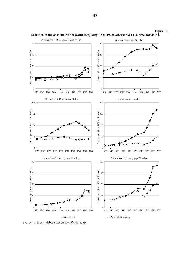
42

Figure 12 Evolution of the absolute cost of world inequality, 1820-1992: Alternatives 1-4, time-variable δδδδ

Alternative 1: Direction of poverty gap

0

10

20

30

40

1820 1840 1860 1880 1900 1920 1940 1960 1980 2000

Percentage ratio to 1992 world median

Alternative 2: Less angular

0

10

20

30

40

1820 1840 1860 1880 1900 1920 1940 1960 1980 2000

Percentage ratio to 1992 world median

Alternative 3: Direction of Kolm

0

25

50

75

100

1820 1840 1860 1880 1900 1920 1940 1960 1980 2000

Percentage ratio to 1992 world median

Alternative 4: Gini-like

0

100

200

300

400

1820 1840 1860 1880 1900 1920 1940 1960 1980 2000

Percentage ratio to 1992 world median

Alternative 5: Poverty gap 1$ a day

0

10

20

30

40

1820 1840 1860 1880 1900 1920 1940 1960 1980 2000

Percentage ratio to 1992 world median

Alternative 6: Poverty gap 2$ a day

0

25

50

75

100

1820 1840 1860 1880 1900 1920 1940 1960 1980 2000

Percentage ratio to 1992 world median

Total Within-country

Source: authors’ elaboration on the BM database..

43

References

Amiel, Y., J. Creedy and S. Hurn (1999). “Measuring Attitudes Towards Inequality”. Scandinavian Journal of Economics, 101, pp. 83-96.

Anand, S., and P. Segal (2008). “What do We Know about Global Income Inequality?”. Journal of Economic Literature, 46, pp. 57-94.

Anand, S., and A. Sen (2000). “The Income Component of the Human Development Index”. Journal of Human Development, 1, pp. 83-106.

Atkinson, A. B. (1970). “On the Measurement of Inequality”. Journal of Economic Theory, 2, pp. 244-263.

Atkinson, A. B. (1973). “More on the Measurement of Inequality”. Mimeo. Published in 2008 in Journal of Economic Inequality, 6, pp. 277-283.

Atkinson, A. B. (1990). “Public Economics and the Economic Public”. European Economic

Review, 34, pp. 225-248. Atkinson, A. B., and F. Bourguignon (1999). “Poverty and Inclusion from a World

Perspective”. In Conseil d’Analyse Économique and The World Bank, Governance,

Equity and Global Markets. Proceedings of the Annual Bank Conference on

Development Economics in Europe, June 21-23 1999, pp. 179-192. Paris: La documentation Française.

Atkinson, A. B., and A. Brandolini (2001). “Promise and Pitfalls in the Use of ‘Secondary’ Data-Sets: Income Inequality in OECD Countries as a Case Study”. Journal of

Economic Literature, 39, pp. 771-799. Atkinson, A. B., and A. Brandolini (2004). “Global World Income Inequality: Absolute,

Relative or Intermediate?”. Paper presented at the 28th General Conference of the International Association for Research in Income and Wealth, Cork, 22-28 August 2004. Available at: http://www.iariw.org/papers/2004/brand.pdf.

Bhagwati, J. (2004). In Defense of Globalization. Oxford University Press, Oxford. Bhalla, S. S. (2002). Imagine There’s No Country. Poverty, Inequality, and Growth in the Era

of Globalization. Washington, D.C.: Institute for International Economics. Blackorby, C., and D. Donaldson (1978). “Measures of Relative Equality and Their Meaning

in Terms of Social Welfare”. Journal of Economic Theory, 18, pp. 59-80. Blackorby, C., and D. Donaldson (1980). “A Theoretical Treatment of Indices of Absolute

Inequality”. International Economic Review, 21, pp. 107-136. Bossert, W., and A. Pfingsten (1990). “Intermediate Inequality: Concepts, Indices, and

Welfare Implications”. Mathematical Social Sciences, 19, pp. 117-134. Bourguignon, F., and C. Morrisson (2002). “Inequality Among World Citizens: 1820-1992”.

American Economic Review, 92, pp. 727-744. Data available at: <www.delta.ens.fr/ XIX>.

Bourguignon, F., V. Levin and D. Rosenblatt (2006). “Global Redistribution of Income”. World Bank Policy Research Working Paper 3961.

Chakravarty, S. R., R. Kanbur and D. Mukherjee (2006). “Population Growth and Poverty Measurement”. Social Choice and Welfare, 26, pp. 471-483.

Chotikapanich, D., D. S. P. Rao and R. Valenzuela (1997). “Global and Regional Inequality in the Distribution of Income: Estimation with Limited and Incomplete Data”. Empirical

Economics, 22, pp. 533-546.

44

Christiansen, V., and E. S. Jansen (1978). “Implicit Social Preferences in the Norwegian System of Indirect Taxation”, Journal of Public Economics, 10, pp. 217-245.

Cowell, F. A. (1980). “On the Structure of Additive Inequality Measures”. Review of

Economic Studies, 47, pp. 521-531. Davies, J. B., and M. Hoy (1985). “Comparing Income Distributions under Aversion to

Downside Inequality”. Mimeo. Deaton, A. (2005). “Measuring Poverty in a Growing World (Or Measuring Growth in a Poor

World)”. Review of Economics and Statistics, 87, pp. 1-19. Del Río, C., and J. Ruiz-Castillo (2000). “Intermediate Inequality and Welfare”. Social Choice

and Welfare, 17, pp. 223-239. Del Río, C., and J. Ruiz-Castillo (2001). “Intermediate Inequality and Welfare: The Case of

Spain, 1980-81 to 1990-91”. Review of Income and Wealth, 47, pp. 221-237. Dollar, D., and A. Kraay (2002). “Growth is Good for the Poor”. Journal of Economic

Growth, 7, pp. 195-225. Dowrick, S., and M. Akmal (2005). “Contradictory Trends in Global Income Inequality: A

Tale of Two Biases”. Review of Income and Wealth, 51, pp. 201-229. Feldstein, M. S. (2005). “Rethinking Social Insurance”. American Economic Review, 95, pp.

1-24. Fields, G. (2006). “Should Poverty and Inequality Measures be Combined?”. In A. de Janvry

and R. Kanbur (eds.), Poverty, Inequality and Development. Essays in Honor of Erik

Thorbecke, pp. 67-74. New York: Springer. Firebaugh, G. (2003). The New Geography of Global Income Inequality. Cambridge, MA:

Harvard University Press. Foster, J. E. (1998). “Absolute versus relative poverty”. American Economic Review, 88, pp.

335-341. Gottschalk, P., and T.M. Smeeding (1997). “Cross-National Comparisons of Earnings and

Income Inequality”. Journal of Economic Literature, 35, pp. 633-687. Kanbur, R. (2008). “Globalization, Growth, and Distribution: Framing the Questions”.

Commission on Growth and Development, Working Paper, No. 5. Kolm, S.-C. (1969). “The Optimal Production of Social Justice”. In J. Margolis and H. Guitton

(eds.), Public Economics. An Analysis of Public Production and Consumption and

Their Relations to the Private Sectors, pp. 145-200. London: Macmillan. Kolm, S.-C. (1976). “Unequal Inequalities. I”. Journal of Economic Theory, 12, pp. 416-442. Little, I. M. D., and J. A. Mirrlees (1974). Project Appraisal and Planning for Developing

Countries. London: Heinemann. Livi Bacci, M. (2001). “Remarks in the Roundtable: ‘Lotta alla povertà nell’economia globale:

un confronto sul World Development Report 2000/2001, Attacking Poverty, della Banca Mondiale’”. QA - La questione agraria, No. 2, pp. 113-116.

Maddison, A. (1995). Monitoring the World Economy. Paris: Organisation for Economic Co-operation and Development.

Maddison, A. (2003). The World Economy: Historical Statistics. Paris: Organisation for Economic Co-operation and Development.

Milanovic, B. (2002). “True World Income Distribution, 1988 and 1993: First Calculation based on Household Surveys Alone”. Economic Journal, 112, pp. 51-92.

Mirrlees, J. A. (1978). “Social Benefit-Cost Analysis and the Distribution of Income”. World

Development, 6, pp. 131-138.

45

Okun, A. M. (1975). Equality and Efficiency. Washington, D.C.: Brookings Institution. Ravallion, M. (2004). “Competing Concepts of Inequality in the Globalization Debate”. In S.

M. Collins and C. Graham (eds.), Brookings Trade Forum 2004. Globalization, Poverty,

and Inequality, pp. 1-38. Washington, DC: Brookings Institution Press. Sala-i-Martin, X. (2006). “The World Distribution of Income: Falling Poverty and …

Convergence, Period”. Quarterly Journal of Economics, 121. pp. 351-397. Sawyer, M. (1976). “Income Distribution in OECD Countries”. OECD Economic Outlook.

Occasional Studies. Paris: Organization for Economic Co-operation and Development, pp. 3-36.

Schultz, T. P. (1998). “Inequality in the Distribution of Personal Income in the World: How It Is Changing and Why”. Journal of Population Economics, 11, pp. 307-344.

Sen, A. K. (1976). “Real National Income”. Review of Economic Studies, 43, pp. 19-39. Sen, A. K. (1983). “Poor, Relatively Speaking”. Oxford Economic Papers, 35, pp. 153-169. Sen, A. K. (1992). Inequality Reexamined. Oxford: Clarendon Press. Sheshinski, E. (1972). “Relation between a Social Welfare Function and the Gini Index of

Inequality”. Journal of Economic Theory, 4, pp. 98-100. Shorrocks, A. F. (1980). “The Class of Additively Decomposable Inequality Measures”.

Econometrica, 48, pp. 613-625. Shorrocks, A. F., and J. E. Foster (1987). “Transfer Sensitive Inequality Measures”. Review of

Economic Studies, 54, pp. 485-497. Stern, N. H. (1977). “Welfare Weights and the Elasticity of the Marginal Valuation of

Income”. In M. J. Artis and A. R. Nobay (eds.), Studies in Modern Economic Analysis:

The Proceedings of the Association of University Teachers of Economics, Edinburgh,

1976. Oxford: Blackwell. Svedberg, P. (2004). “World Income Distribution: Which Way?”. Journal of Development

Studies, 40, pp. 1-32. United Nations Development Programme (1991). Human Development Report 1991. Oxford:

Oxford University Press. US Census Bureau (2000). The Changing Shape of the Nation’s Income Distribution.

Washington, DC: US Department of Commerce. World Bank (2008). Global Purchasing Power Parities and Real Expenditures. 2005

International Comparison Program. Washington, D.C.: The World Bank. Zheng, B. (2004). “On Intermediate Measures of Inequality”. In Y. Amiel and J. A. Bishop

(eds.), Research on Economic Inequality. Vol. 12: Studies on Economic Well-Being:

Essays in the Honor of John P. Formby, pp. 135-157. Oxford: Elsevier. Zheng, B. (2007). “Unit-Consistent Decomposable Income Measures”. Economica, 74, pp.

97-111. Zoli, C. (1999). “A Generalized Version of the Inequality Equivalence Criterion: a Surplus

Sharing Characterization, Complete and Partial Orderings”. In H. de Swart (ed.), Logic,

Game Theory and Social Choice, pp. 427-441. Tilburg: Tilburg University Press.