Embed Size (px)
Citation preview

Oligopoly (Game Theory)

Oligopoly: Assumptions
Many buyers Very small number of major sellers
(actions and reactions are important) Homogeneous product (usually, but not
necessarily) Perfect knowledge (usually, but not
necessarily) Restricted entry (usually, but not
necessarily)

Oligopoly Models
1. “Kinked” Demand Curve
2. Cournot (1838)
3. Bertrand (1883)
4. Nash (1950s): Game Theory

“Kinked” Demand Curve
P
Q or q
Elastic
Inelasticp*
Q* or q*
D or d

“Kinked” Demand Curve
P
Q or q
Elastic
Inelasticp*
Q* or q*
Where do p* and q* come
from?
D or d

Cournot Competition
Assume two firms with no entry allowed and homogeneous product
Firms compete in quantities (q1, q2) q1 = F(q2) and q2 = G(q1) Linear (inverse) demand, P = a – bQ where
Q = q1 + q2
Assume constant marginal costs, i.e.
TCi = cqi for i = 1,2 Aim: Find q1and q2 and hence p, i.e. find the
equilibrium.

Cournot Competition
Firm 1 (w.o.l.o.g.)
Profit = TR - TC
1 = P.q1 - c.q1
[P = a - bQ and Q = q1 + q2, hence
P = a - b(q1 + q2)
P = a - bq1 - bq2]

Cournot Competition
1 = Pq1-cq1
1 =(a - bq1 - bq2)q1 - cq1
1 =aq1 - bq12 - bq1q2 - cq1
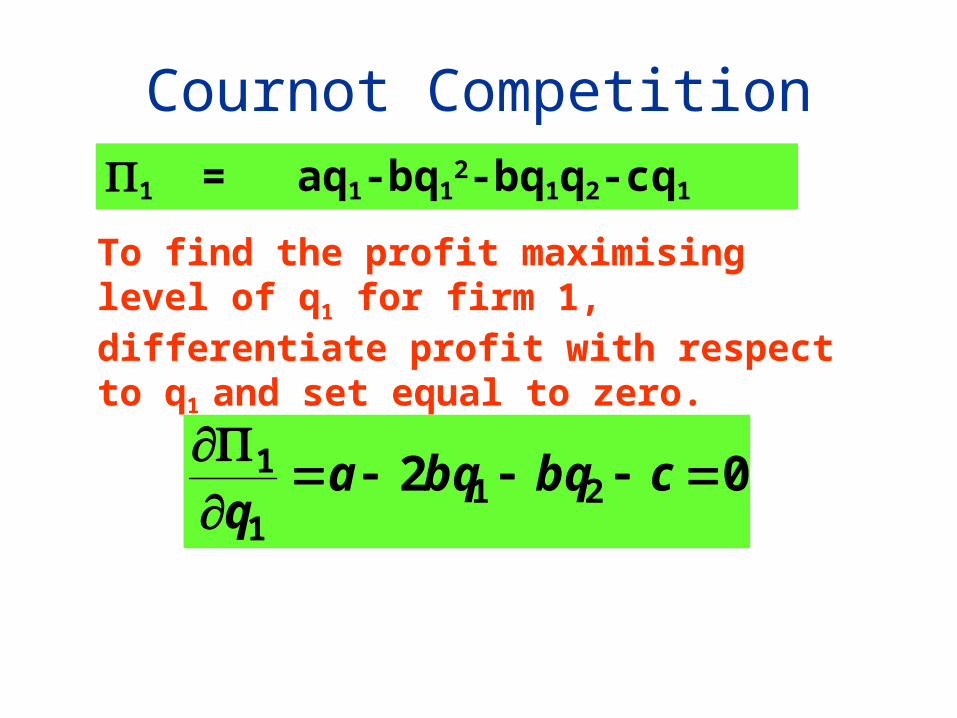
Cournot Competition1 = aq1-bq1
2-bq1q2-cq1
To find the profit maximising level of q1 for firm 1, differentiate profit with respect to q1
and set equal to zero.
02 211
1
cbqbqaq

Cournot Competition
02 21 cbqbqa
acbqbq 212
cabqbq 212
212 bqcabq
b
bqcaq
22
1
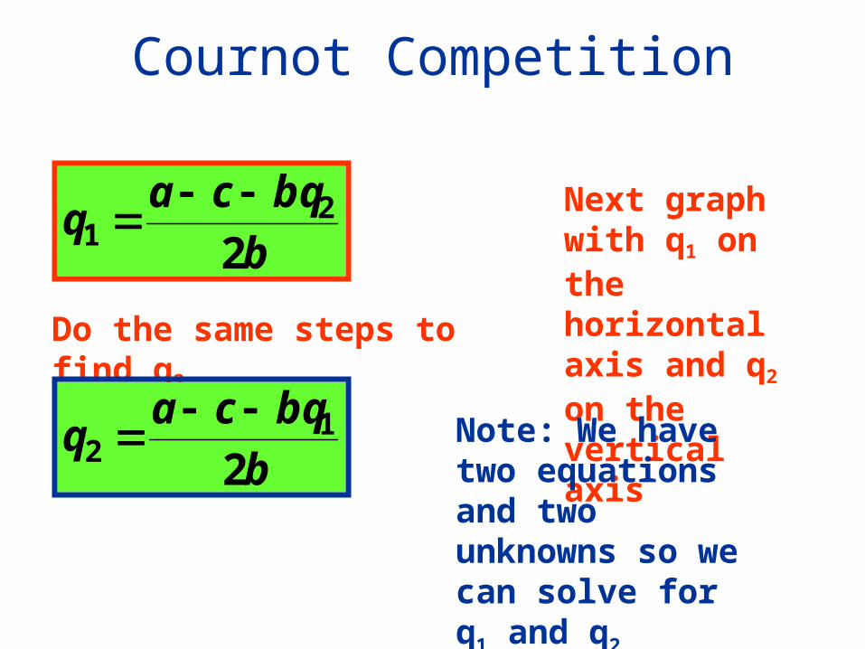
Firm 1’s “Reaction” curve
Cournot Competition
b
bqcaq
22
1
Do the same steps to find q2
b
bqcaq
21
2
Next graph with q1 on the horizontal axis and q2 on the vertical axis
Note: We have two equations and two unknowns so we can solve for q1 and q2

Cournot Competition
b
bqcaq
22
1
q2
q1
b
bqcaq
21
2
COURNOT EQUILIBRIUM

Cournot Competition
b
bqcaq
22
1
b
bqcaq
21
2
Step 1: Rewrite q1
b
bq
b
c
b
aq
2222
1
Step 2: Cancel b
2222
1q
b
c
b
aq
Step 3: Factor out 1/2
21 2
1q
b
c
b
aq
Step 4: Sub. in for q2
b
bqca
b
c
b
aq
22
1 11

Cournot Competition
Step 5: Multiply across by 2 to get rid of the fraction
b
bqca
b
c
b
aq
22
1 11
b
bqca
b
c
b
aq
2112 1
1
Step 6: Simplify
2222 1
1q
b
c
b
a
b
c
b
aq

Cournot Competition
Step 7: Multiply across by 2 to get rid of the fraction
Step 8: Simplify
2222 1
1q
b
c
b
a
b
c
b
aq
2
2
2
2
2
2224 1
1q
b
c
b
a
b
c
b
aq
1122
4 qb
c
b
a
b
c
b
aq

Cournot Competition
Step 9: Rearrange and bring q1 over to LHS.
Step 10: Simplify
1122
4 qb
c
b
a
b
c
b
aq
b
c
b
c
b
a
b
aqq
224 11
b
c
b
aq 13 Step 11: Simplify
b
caq
31

Cournot CompetitionStep 12: Repeat above for q2
b
caq
31
Step 13: Solve for price (go back to demand curve)
bQaP
b
ca
b
cabaP
33
Step 14: Sub. in for q1 and q2
b
caq
32

Cournot Competition
b
ca
b
cabaP
33
33
cacaaP
3333
cacaaP
Step 14: Simplify

Cournot Competition
3333
cacaaP
ccaaaP3
1
3
1
3
1
3
1
caaP3
2
3
2 caP
3
2
3
1
3
2caP

Cournot Competition: Summary
b
caq
31
b
caq
32
b
ca
b
caQ
33
b
caQ
3
2

Cournot v. Bertrand
Cournot Nash (q1, q2): Firms compete in quantities,
i.e. Firm 1 chooses the best q1 given q2 and
Firm 2 chooses the best q2 given q1
Bertrand Nash (p1, p2): Firms compete in prices,
i.e. Firm 1 chooses the best p1 given p2 and
Firm 2 chooses the best p2 given p1
Nash Equilibrium (s1, s2): Player 1 chooses the best s1 given s2 and Player 2 chooses the best s2 given s1

Bertrand Competition: Bertrand Paradox
Assume two firms (as before), a linear demand curve, constant marginal costs and a homogenous product.
Bertrand equilibrium: p1 = p2 = c
(This implies zero excess profits and is referred to as the Bertand Paradox)

Perfect Competition v. Monopoly v. Cournot Oligopoly
ii cqTCandbQaP
Perfect Competition
b
caQCPMCP pc
Given
Monopoly
CQbQaQ
CQQbQa
CQPQ
TCTR
2

Perfect Competition v. Monopoly v. Cournot Oligopoly
02
2
CbQaQ
CQbQaQ
b
CaQ
CabQ
m
2
2
2
2
CaP
b
CabaP
bQaP
M

Perfect Competition v Monopoly v Cournot Oligopoly
b
caQCO
3
2
3
2caPCO
Qm < Qco < QPC
Pm > Pco > Ppc