Chapter 13

Oligopoly and Monopolistic Competition

©2015 McGraw-Hill Education. All Rights Reserved. 2

Chapter Outline

• Some Specific Oligopoly Models • Competition When There are Increasing Returns to

Scale• Monopolistic Competition• A Spatial Interpretation of Monopolistic

Competition• Historical Note: Hotelling’s Hot Dog Vendors• Consumer Preferences and Advertising

©2015 McGraw-Hill Education. All Rights Reserved. 3

The Cournot Model

• Cournot model: oligopoly model in which each firm assumes that rivals will continue producing their current output levels.– Main assumption - each duopolist treats the

other’s quantity as a fixed number, one that will not respond to its own production decisions.

©2015 McGraw-Hill Education. All Rights Reserved. 4

Figure 13.1: The Profit-Maximizing Cournot Duopolist

©2015 McGraw-Hill Education. All Rights Reserved. 5

The Cournot Model

• Reaction function: a curve that tells the profit-maximizing level of output for one oligopolist for each amount supplied by another.

©2015 McGraw-Hill Education. All Rights Reserved. 6

Figure 13.2: Reaction Functionsfor the Cournot Duopolists

©2015 McGraw-Hill Education. All Rights Reserved. 7

Figure 13.3: Deriving the Reaction Functions for Specific Duopolists

©2015 McGraw-Hill Education. All Rights Reserved. 8

The Bertrand Model

• Bertrand model: oligopoly model in which each firm assumes that rivals will continue charging their current prices.

©2015 McGraw-Hill Education. All Rights Reserved. 9

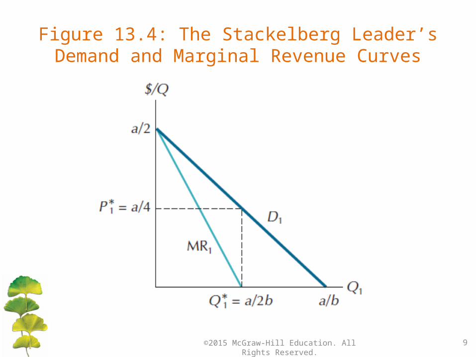
Figure 13.4: The Stackelberg Leader’s Demand and Marginal Revenue Curves

©2015 McGraw-Hill Education. All Rights Reserved. 10

Figure 13.5: The Stackelberg Equilibrium

©2015 McGraw-Hill Education. All Rights Reserved. 11

Table 13.1: Comparison Of Outcomes

©2015 McGraw-Hill Education. All Rights Reserved. 12

Figure 13.6: Comparing Equilibrium Price and Quantity

©2015 McGraw-Hill Education. All Rights Reserved. 13

Competition When There Are IncreasingReturns To Scale

• In markets for privately sold goods, buyers are often too numerous to organize themselves to act collectively. – Where it is impractical for buyers to organize

direct collective action, it may nonetheless be possible for private agents to accomplish much the same objective on their behalf.

©2015 McGraw-Hill Education. All Rights Reserved. 14

Figure 13.7: Sharing a Market with Increasing Returns to Scale

©2015 McGraw-Hill Education. All Rights Reserved. 15

The Chamberlin Model• Assumption: a clearly defined “industry group,”

which consists of a large number of producers of products that are close, but imperfect, substitutes for one another.

• Two implications:1. Because the products are viewed as close substitutes,

each firm will confront a downward-sloping demand schedule.

2. Each firm will act as if its own price and quantity decisions have no effect on the behavior of other firms in the industry.

©2015 McGraw-Hill Education. All Rights Reserved. 16

Figure 13.8: The Monopolistic Competitor’s Two Demand Curves

©2015 McGraw-Hill Education. All Rights Reserved. 17

Figure 13.9: Short-Run Equilibrium for the Chamberlinian Firm

©2015 McGraw-Hill Education. All Rights Reserved. 18

Figure 13.10: Long-Run Equilibriumin the Chamberlin Model

©2015 McGraw-Hill Education. All Rights Reserved. 19

Perfect Competition Versus ChamberlinianMonopolistic Competition

• Competition meets the test of allocative efficiency, while monopolistic competition does not.

• Monopolistic competition is less efficient than perfect competition because in the former case firms do not produce at the minimum points of their long-run average cost (LAC) curves.

• In terms of long-run profitability the equilibrium positions of both the perfect competitor and the Chamberlinian monopolistic competitor are precisely the same.

©2015 McGraw-Hill Education. All Rights Reserved. 20

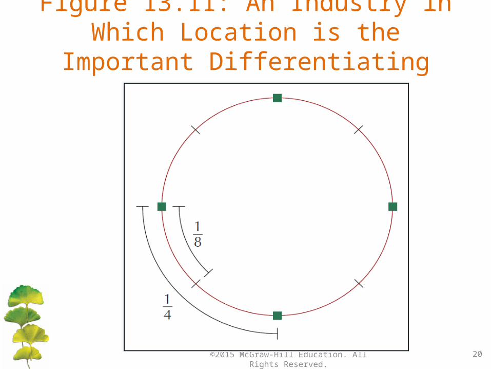
Figure 13.11: An Industry in Which Location is the Important Differentiating Feature

©2015 McGraw-Hill Education. All Rights Reserved. 21

The Optimal Number of Locations• The number of outlets that emerges from the

independent actions of profit-seeking firms will in general be related to the optimal number of outlets in the following simple way:– Any environmental change that leads to a change in the

optimal number of outlets (here, any change in population density, transportation cost, or fixed cost) will lead to a change in the same direction in the equilibrium number of outlets.

©2015 McGraw-Hill Education. All Rights Reserved. 22

Figure 13.12: Distances with N Outlets

©2015 McGraw-Hill Education. All Rights Reserved. 23

Figure 13.13: The Optimal Numberof Outlets

©2015 McGraw-Hill Education. All Rights Reserved. 24

Figure 13.14: A Spatial Interpretationof Airline Scheduling

• Why not have a flight leaving every 5 minutes, so that no one would be forced to travel at an inconvenient time?

• The larger an aircraft is, the lower its average cost per seat is.

• If people want frequent flights, airlines are forced to use smaller planes and charge higher fares.

©2015 McGraw-Hill Education. All Rights Reserved. 25

Figure 13.15: Distributing the Costof Variety

©2015 McGraw-Hill Education. All Rights Reserved. 26

Figure 13.16: The Hot Dog Vendor Location Problem

©2015 McGraw-Hill Education. All Rights Reserved. 27

Consumer Preferences And Advertising

• Because products are differentiated, producers can often shift their demand curves outward significantly by advertising.

• The revised sequence: the corporation decides which products are cheapest and most convenient to produce, and then uses advertising and other promotional devices to create demand for them.